tehneai~ le e h ia report
TRANSCRIPT

' ~ ~ TEHNEA
le E H IA REPORTNo. 12.590
I~ u-I
ANALYSIS OF MECHANICAL SYSTECS HL
Final Report
16 June 1981'1, S
Contract No: DAAK30-78-C-O096 !DAAG29-79-C-0221
College of Engineering,
~University of Iowa
University of Iowa Report No. 75m
by %mb ,o.P*4.eg.n-r A
Approved for public relese; distribution unlimited,
U.S. ARMY TANK-AUTOMOTIVE COMMAND.RESEARCH AND DEVELOPMENT CENTERWarme, Michimn 48090
81 12 17064
II,I .) ,, , . ... . . . ,:-- _ - " ' ..,. .. .. . . .. .
I

DISCLAIMER NOTICE
THIS DOCUMENT IS BEST QUALITYPRACTICABLE,. THE COPY FURNISHEDTO DTIC CONTAINED A SIGNIFICANTNUMBER OF PAGES WHICH DO NOTREPRODUCE LEGIBLY.

NOTICES
The findings in this report are not to be construed as an official Departmentof the Army position.
Mention of any trade names or manufacturers in this report shall not beconstrued as advertising nor as an official endorsement of approval of suchproducts or companies by the U.S. G'vernment.
Destroy this report when it is. no longer needed. Do not return it tooriginator.

,ECURITY CLASSIFICATION OF THIS PAGE (When Dawo lOtered)
READ INSTRUCTIONSREPORT DOCUMENTATION PAGE BEFORE COMPLETING FORM
1. REPORT NUMBER 2. GOVT ACCESSION NO. 3. RECIPIENT'S CATALOG NUMBER
12590 4 / o 34. TITLE (and Subtitle) S. TYPE OF REPORT & PERIOD COVERED
Generalized Coordinate Partitioning in Final, Dec. 1980Dynamic Analysis of Mechanical Systems . PERFORMING ORG. REPORT NUMBER
1---AU O )" . CONTRACT OR GRANT NUMBER(e)
R KA Wehage and E J. Haug DAAK30-78-C-0096
University of Iowa DAAG29-79-C-0221Ronald R. Beck, TACOM
9, PERFORMING ORGANIZATION NAME AND ADDRESS 10. PROGRAM ELEMENT. PROJECT. TASK
AREA & WORK UNIT NUMBERSThe University of Iowa
College of EngineeringIowa City, IA 52242
I 1- CONTROLLING OFFICE NAME AND ADDRESS 12. REPORT DATE
U.S. Army Tank-Automotive Command, R&D Center 16 June 1981Tank-Automotive Concepts Lab, DRSTA-ZSA 13 NUMBER OF PAGES
Warren, MI 48090 20514. MONITORING AGENCY NAME & ADVRESS(II different from Controlling Office) 15. SECURITY CLASS. (of thle report)
Unclassified
15. DECL ASSI FIC ATION DOWN GRADINGSCHEDULE
16 DISTRIBUTION STATEMENT (of ths Report)
Approved for public release; distribution unlimited.
17. DISTRIBUTION STATEMENT (of the abelrct enteted In Block 20, It different from Report)
19 SUPPLEMENTARY NOTES
III KEY WORDS (Cortinue on revree side If neceeeary nd Identify by block number)
Matrices, Sparse Matrix, Dynamics, Bodies Response Control,Interaction, Stability, Lagrangian Functions
20. A1IT RACr (centare - rever e eib If neey mi Ideftl ly by block number)
A computer-based method for formulation and efficient solution of nonlinear,constrained differential equations of motion is developed for planar mechanical
systems. Nonlinear holonomic constraint equations and differential equations ofmotion are written in terms of a maximal set of Cartesian generalized coordinates,to facilitate the general formulation of constraints and forcing functions. A
Gaussian elimination algorithm with full pivoting decomposes the constraintJacobian matrix, identifies dependent variables, and constructs an influencecoefficient matrix relating variations in dependent and independent variables.
DO "0 ,o,, 43 EDI TION OF,,M1OV &$IS O8WLE, / .DO I iM 73 UNCLASSIFIED ,
SECUIrYTV CLASSIFICATION OF YHIS PAGE (Wfen Dae Entered)

UNCLASSIFIEDSECURITY CLASSIFICATION OF THIS PAGE(Whm Det Entered)
This information is employed to numerically construct a reduced system ofdifferential equations whose solution yields the total system dynamic response.A numerical integration algorithm with positive-error control, employing apredictor-corrector algorithm with variable order and step-size, is developedthat integrates for only the independent variables, yet effectively determinesdependent variables.
A general method is developed for dynamic analysis of systems with impulsiveforces, impact, discontinuous constraints, and discontinuous velocities. Thisclass of systems includes discontinuous kinematic and geometric constraints thatcharacterize backlash and impact within systems. A method of computer generationof the impulse-momentum relations that define jump discontinuities in systemvelocity for large scale systems is developed. An event predictor employinglogical functions of system state and working in conjunction with the new numeri-cal integration algorithm efficiently controls its progress and allows for auto-matic equation reformulation.
Numerical results are presented for planar motion of a tracked articulatedvehicular system with twenty-four degrees of freedom. A mechanism with discon-tinuous forces and velocities is simulated to demonstrate program generality andimproved efficiency over previous modeling methods. An order of magnitudeimprovement in efficiency has been demonstrated.
SECURITY CLASSIFICATION OF THIS PAGOE(*en Date Entered

LIA0ee33ion Ior
ABSTRACT&
A computer-based method for formulation and efficient solution
of nonlinear, constrained differential equations of motion is
developed for planar mechanical systems. Nonlinear holonomic con-
straint equations and differential equations of motion are written
in terms of a maximal set of Cartesian generalized laoordinates, to
facilitate the general formulation of constraints and forcing fun-
tions. A Gaussian elimination algorithm with full pivoting
decomposes the constraint Jacobian matrix, identifies dependent
variables, and constructs an influence coefficient matrix relating
variations in dependent and indepen t variables. This information
is employed to numerically construct a reduced system of differential
equations whose solution yields the total system dynamic response.
A numerical integration algorithm with positive-error control,
employing a predictor-corrector algorithm with variable order and
step-size, is developed that inte-ates for only the independent
variables, yet effectively determines dependent variables.
A general method is developed for dynamic analysis of systems
with impulsive forces, impact, discontinuous constraints, and dis-
continuous velocities. This class of systems includes discontinuous
kinematic and geometric constraints that characterize backlash and
impact within systems. A method of computer generation of the
I!

Impulse-momentum relations that define jump discontinuities in system
velocity for large scale systems is developed. An event predictor
employing logical functions of system state and working in conjunction
with the new numerical integration algorithm efficiently controls
its progress and allows for automatic equation reformulation.
Numerical results are presented for planar motion of a tracked
articulated vehicular system with twenty-four degrees of freedom. A
mechanism with discontinuous forces and velocities is simulated
to demonstrate the capabilities of the method. The examples were
selected to demonstrate program generality and improved efficiency
over previous modeling methods. An order of magnitude improvement
in efficiency has been demonstrated.
li

TABLE OF CONTENTS
Page
ABSTRACT . . . . . . . . . . . . . . . . . . . . . . . . . i
LIST OF TABLES ...................... v
LIST OF FIGURES ....... ..................... ..... vi
LIST OF SYMBOLS.......... ...................... viii
CHAPTER
1. INTRODUCTION .... ..... .................. 1
1.1 Introductory Comments ...... ........... 11.2 Program Efficiency Versus Program
Generality .... .... ................ 21.3 Obtaining Efficiency Without Sacrificing
Generality ... .... ................ 61.4 Scope of the Report ...... ............ 9
2. THE PLANAR RIGID BODY MODELING METHOD FORCONSTRAINED SYSTEMS .............. 16
2.1 Introduction .... .............. .. 162.2 Constrained Equations of Planar Motion • 192.3 Integpation of Constrained Equation of
Motion by an Implicit Method ....... .31
3. KINEMATIC ANALYSIS AND GENERALIZED COORDINATEPARTITIONING FOR DIMENSION REDUCTION IN ANALYSISOF CONSTRAINED RIGID BODY SYSTEMS .... ....... 38
3.1 Introduction ... ............... ... 383.2 System Constraints .. ........... ... 403.3 Kinematic Velocity and Acceleration
Analysis .............. 493.4 Kinetostatics of Constrained Systems • • 523.5 Sparse Matrix Considerations . . . . . . . 57
4. CONSTRAINED EQUILIBRIUM AND DYNAMIC ANALYSIS . . 63
4.1 Introduction . ............... 634.2 Equilibrium Analysis . ........... ... 64
iii

CHAPTER Page
4.3 Initial Conditions ............ 674.4 Numerical Integration of the Equations
of Motion .... ................. .... 694.5 Sparse Matrix Considerations ... ....... 74
5. PIECED INTERVAL ANALYSIS ............ . 80
5.1 Introduction ............ ... 805.2 Logical Events Monitor for Pieced
Interval Analysis .... ............ .... 825.3 Intermittant Motion in Constrained
Systems ..... .................. ... 865.4 Pieced Interval Ccmputational Algorithm . . 925.5 Spars,. Matrix Considerations ... ....... 94
6. NUMERICAL EXAMPLES ....... ............... 98
6.1 Introduction ..... ......... 986.2 Two Articulated Army M-1U3 Armored
Personnel Carriers ... ............ .. 1026.3 A Mechanism With Intermittent Motion . . . 139
7. CONCIUSIONS AND RECOMMENDATIONS ........ ... 160
7.1 Conclusions..... . . . . . . . . . . 1607.2 Recommendations .............. 161
APPENDIX A. RANK DETERMINATION AND DECOMPOSITION OFSINGULAR MATRICES .............. 165
REFERENCES ......... ....................... ... 177
iv

LIST OF TABLES
Table Page
1.1 Comparison of features of some general purpose
c nputer codes . . . ................. 4
-
V It
_________'

p II I
LIST OF FIGURES
Figure Page
2.1. Rigid bodies connected by a vector r and
rotational joints ...... .................... 20
2.2. Rigid bodies connected by a translational joint . . 23
2.3. Rigid bodies connected by a spring-damper-actuatorcombination ...... ................... ..... 26
5.1. Various combinations of logical variable and itsderivative at times tn and tn+1 .............. ... 85
5.2. Event interval ....... ................. .... 87
5.3. Impacting bodies ..... .................. .... 89
6.1. Link gear multiplier ...... .. ................ 100
6.2. Peaucellier Lipkin mechanism ... ............ ... 101 I6.3. Coupled Mll3's ...... ................... .... 103
6.4. A computer model of the coupled Mll3's ... ....... 108
6.5. Torsion bar suspension characteristics ... ....... 109
6.6. Suspension damping characteristics .... ......... 109
6.7. Roadwheel-ground force--penetration curve ..... . 113
6.8. Terrain contour of 36 inch step obstacle ... ...... 115
6.9. Trajectory of 12 inch wheel rolled over a 36 inchstep obstacle ...... .... .................. 116
6.10. Wheel trajectory defined by lowest points on wheelwith no terrain penetration ...... ............ 117
6.11. Direction of a line passing through point of wheel-terrain contact and wheel center .. .......... ... 119
6.1 Terr n-wheel contact forces .. ............ .... 120
VI

Figure Page
6.13. Control system diagram ..... .............. ... 125
6.14. Control stick and force actuator .. .......... ... 128
6.15. Obstacle crossing with force and position feedbackactive - ten second simulation at 40 inches/second . 131
6.16. Obstacle crossing with force feedback deactivated -ten second simulation at 40 inches/second .... . 132
6.17. Obstacle crossing with the control systemdeactivated - ten second simulation at 40inches/second ......... ................... 133
6.18. System hydraulic actuator pressure .. ......... ... 135
6.19. Angular displacement of the control stick(negative = pitch-up) .................... ... 136
6.20. Hydraulic pump yoke displacement (percent fullstroke) ............ ................... 136
6.21. Cannon system shown in positions where barrel leavesor impacts sear ...... .................. ... 142
6.22. Position where sleeve starts to move rearward withrespect to barrel or comes to rest with respect toreceiver ........ ...................... .... 144
6.23. Position where rearward motion of the sleeve withrespect to barrel ceases or begins .. ......... ... 145
6.24. Position where barrel contacts or leaves frontBuffer ........ ....................... .... 146
6.25. Firing position ...... .................. ... 147
6.26. Barrel assembly at rearmost position .......... .. 1148
6.27. Horizontal displacement of the gun tube ...... . 156
6.28. Horizontal velocity of the gun tube . ........ . 157
6.29. Horizontal acceleration of the gun tube ...... . 158
A.l. Format scheme of the processed matrix .. .... . 176
vii

LIST OF SYMBOLS
Symbol
A Composite vector of Ai
Ai Velocity dependent terms for the ith body resulting
from differentiating Ti with respect to t and qi
Au , AV Partitioning of A according to u and v
A Actuator area - rod end
A2 Actuator area - cylinder end
Bi Rigid body numbers
Bf Constant front buffer force
B Constant rear buffer forcer
CI Angular, centripetal, and Coriolis acceleration dueto independent constraints
C2 Angular, centripetal, and Coriolis acceleration due
to redundant constraints
C. Damping CoefficientIQ
dof System degree of freedom
D W. Damping force developed on ith wheel due toI interaction between wheel and terrain
dl, d2 Upper and lower lengths of the control stick
e Coefficient of restitution
E(s) Error signal voltage in control system
f Vector of functions
f(t) Impulsive force acting at contacting surfacesduring impact
viii

Symbol
F' Force developed in successive track segments afterbeing reduced by friction forces
f B Functional relation between pin P and barrel B inweapon system
F. Constant force driving the barrel rearward0
Fd Vehicle suspension damping fcr.e function of (- ij)
Ff Constant force drivi • barrel forward
Ff IFriction force acting tangent to the heel-terrainf contact surface where IF[ < IFfj when the wheel
does not slide
F Ffy Projection of frictional force Ff along x and y
axes respectively
Force vector in the spring-damper-actuator
F Normal force acting between roadwheel and terrainn surface
F , F Projection of F along x and y axes respectivelyn ny n
f R Functional relation between pin P and receiver Rin weapon system
F R(s) Operator supplied fore and aft force to the controlstick
F (F w) Total vertical force acting upward on a wheel at1 the point of wheel-terrain contact
F s(A0 - )ij Vehicle suspension force functionij
Fu Fv Partitioning of generalized constraint reactionforces according to u and v
F (Fs) Force developed on a wheel due to interactionbetween wheel and terrain
Fx , F Projection of Fij on the x and y axes respectively
ix

Symbol
F (s) Plnp yoke limiting forceY
FO Actuator force applied along the spring-damper-
1J actuator element
g Vectors of functions
g(x) A function that defines terrain or wheel trajectoryelevation as a function of the wheel's global xposition
h Time step in the multistep integration formulas
h(x) A function that defines the angular position of avector passing through the point of wheel-terraincontact and center of wheel
H Influence coefficient matrix
H The matrix H evaluated at points in (', T 2 )
1) J Unit vectors parallel to the x and y axes,
respectively
I Identity matrix
T Rectangular matrix of full row rank consisting ofa null and I matrix when columns are permutedaccording to u and v
I(s) Amplifier current
J Jacobian matrix defined in Equation 2.33
J. Centroidal polar moment of inertia of the ith body
k Degree of a polynomial in the multistep integrationformula
k'F Number of logical times
K K Constants that characterize a vehicle power traind v
Ki Measure of velocity ratios
kij Spring constant
x

Symbol
KRp Rotational potentiometer gain
K Servo valve flow gradientv
KI, K2 Amplifier gain
K1 , K2 Springs attached to the lower part of the controlstick
K 3 Pump stroke mechanism velocity gradient
K4 Actuator potentiometer feedback gain
L Combined system leakage coefficient
L, U Lower and upper triangular matrices. In permutedform L • U = I
I ij Deformed spring length
I iThe jth logical variable
to023 Reference hydraulic actuator length
123 Total hydraulic actuator length
to iUndeformed spring length
LR, UR Residual lower and upper matrices. In permutedform L • UR = §v
m Number of constraint equations
M Composite system mass matrix
m' Number of logical functions
Mass matrix of the ith body
m, Mass of the i t h body
Muu Muv Partitioning of the mass matrix according to uM vU MvV and v
n Number of system rigid bodies
xi

Symbol
7Row vector that determines the relative velocitydirection in an internal impact
N Row vector that relates generalized velocitiesduring internal impact
NU NV Partitioning of N according to u and v
p Magnitude of impulse acting at contacting surfacesduring impact
P Vector of generalized impulses
P(s) System pressure at the actuatorth
pi The i roadwheel penetration into the terrain
Pij' Pji L Points located on the ith and j bodiesPil'Pjli respectively
Pi2' Pj2 jpu v Generalized impulses P partitioned according to
u and v
q Composite vector of all system generalized
coordinates
Composite vector of all system generalized forces
4(ti-) System velocity before a discontinuous event at t i
j(t i +) System velocity after a discontinuous event at t.
QA Actuator flow rate
QC Flow due to compressibility
q Vector of generalized coordinates of body i
q q Values of system generalized coordinates and
velocities at ti
Qi Vector of generalized forces on body i
xii

Symbol
Aui Discontinuous change in velocity at t.
qj' ik The jth element of q, the kth element of i
QL Leakage flow
Qp Pump flow gradient
QT Pump flow
U QV Partitioning of Q according to u and v
Q V* Known generalized forces corresponding to thespecified independent (v) generalized coordinatesin a displacement driven system
Qi Q i Qi Generalized forces on body i corresponding toX Y C generalized coordinates x., y,, and Ti,
respectively
i i iQi Qi Generalized forces on body i due to a spring-Qx 'yss Ys Ys damper-actuator combination
r Number of independent algebraic constraint equations(rank of the constraint Jacobian matrix)
R(s) Reference voltage signal from the control stickpotentiometer
i Vector locating the origin of the coordinate
system fixed in the ith body
r ijrVectors locating points on the i and j bodies,
respectively, with respect to body fixed coordinatesystems
4 .thr Vector locating the center of mass cn the i body
i with respect to body fixed coordinate system
r Vector between two points on adjacent bodiesP
"rsj Tracked vehicle sprocket radius
-4 1r , r Vectors locating spring-damper-actuator attachments ij s ji points on the ith and jth bodies, respectively,
with respect to body fixed coordinate systems
xiii

Symbol
1Vector between spring-damper-actuator attachmentij points on two bodies
Rv Unknown driving generalized forces correspondingto specified independent (v) generalized coordinatesin a displacement driven system
r Roadwheel radiusw
s s E v -- Introduced to reduce equations of motionto first order form
,t, i. Vectors connecting points (p il Pi2 ), (p.il Pj2 )
and (pj' Pil ) on the i t h and jth body,
respectively
s.. Points located on the ith and jth bodies3ij 1 j respectively
si Time derivative of the jth logical variable
Sj Spring-damper-actuator numbers
S. Actual displacement of a reference point on thej vehicle
S r. Total desired displacement of a reference pointon the vehicle, along the terrain
S O Initial global location of a reference point onthe vehicle
Slip A number > 0 if the wheel slides in the positive
x direction and < 0 if the wheel slides in thenegative x direction
T i Kinetic energy of the ith body
t i - Approaches an event at ti from t < t i
t.+ Approaches an event at t i from t > t i1
T. Track driving force developed by the power train
T L(S) Control stick limiting torque
xiv

Symbol
Tq, T. Partial derivative of kinetic energy with respectq to generalized coordinates and velocities
u, v Partitioning of q into dependent and independentvariables, respectively
u* Change in dependent generalized coordinates u due
to time dependence of §
i* Change in dependent generalized velocities i due
to time dependence of §
jj* Change in dependent generalized accelerations U
due to angular, centripetal, and Coriolis effectsof constraints
i iu ,v Values of dependent and independent generalized
coordinates at t.1
vj Actual velocity of a reference point on the vehicle
vp , sP Predicted values of v and s
vr Desired velocity of a reference point on thevehicle
S JS . Specified independent generalized coordinates,
velocities, and accelerations in a displacementdriven system
V 0 Entrained volume of hydraulic fluid
v23 (s) Actuator velocity
w w. a -- Generalized velocity vector introduced toreduce equations of motion to first order
x, y Inertial reference frame
XB' YB Global location of the barrel
xi'9 Yi Global coordinates of the origin of the ith bodyfixed coordinate system
thXm , y Global coordinates of the i body center of mass
xp, y Global location of the pin in the weapon system
xv

Symbol
x, y Global location of a point on the jth bodyP.p
x1, yi Global location of the receiver in the weaponsystem
Y(s) Pump yoke displacement
z(s) Actuator displacement
Q Angle between a spring-damper-actuator and theinertial reference frame
C = h(x)
cj' I 0 Gear's coefficients
e Effective bulk modulus including system compliance
8 Force unbalance tolerance
8Wi Virtual work of forces acting on the i t h body
E Constraint closure tolerance
e (s) Angular displacerent of control stick
X Lagrange multiplier vector that determinesconstraint reaction forces
Vector of Lagrange multipliers that determineconstraint reaction impulses
2 Lagrange multipliers corresponding to independent
and dependent constraint equations
Coefficient of friction
mi Body-fixed coordinate systems in the ith body
~btij, I ij
il' 'il Components of the vectors, 2 and
9i2' 'i2 respectively, in the C, " 1i coordinate system
9sij isjii
xvi

1ji' ji
Ijl' jl Components of the vectors rji' rjl'p j2' and r ,sji
[j2' J2 respectively, in the C. - coordinate system
Ai ji
Cmi, 11mi Cc:r.ponents of the vector r in the ,- f
-oordinate system
TControl system time constantC
l 1 Servo valve time constant
T 1' T2 Small time interval containing a discontinuousevent
Vector of equations of constraint between bodies
Ti Angle between the inertial reference x-axis andbody-fixed i-axis
q Constraint Jacobian matrix
(boi/bqj
Sq Nonsingular matrix composed of §q and I
*t' 'tt Partial derivatives of constraints with respect toq tt time and generalized coordinates
u' v Partial derivatives of constraints with respect todependent and independent variables, respectively
1 Independent constraint equations
2 Dependent or redundant constraint equations
nJ The jth logical function
cond( ) Condition number of a matrix
8( ) A virtual change in the indicated quantity
A( ) A small change in the indicated quantity
xvii

II
Symbol
( ), ( ) Differentiation with respect to time
2H " The I norm of a vector
)T Transpose of a vector or matrix
( )-T Inverse of the transpose of a matrix
( )-i Inverse of a matrix
xviii

1
CHAPTER 1
INTRODUCTION
1.1 Introductory Comments
Analysis of machine and mechanism problems prior to 1960
relied upon various (and often quite complex) graphical techniques.
These techniques were based on geometrical interpretation of con-
straints and a large body of literature evolved which classified
constraints and linkages [1, 23. In the 1950's digital and analog
computers began to appear, making it possible to formulate and
repetitively solve moderately sized systems of equations [3, 4j.
This prompted the development of mathematical software support
packages and the possibility of mathematical analysis of machines
and vehicular systems became a reality. The early programs, written
specifically for given applications, used geometrical interpretation
of constraints to define relative position coordinates, thus helping
to reduce problem size. These programs were generally limited in
scope, requiring extensive modification for different applications
[5, 6].
As computer speed and capacity increased, larger programs
were developed, along with data handling routines. It was recognized
that mechanical systems are composed of a number of "standard"
elements and that they can be combined as building blocks to define
2
large classes of mechanisms. Again, geometrical interpretation of
constraints allowed for the reduction in the number of independent
variables, so that considerably larger, more sophisticated models
could be established. However, the methods developed required top-
ological analysis associated with identification of independent con-
straint loops, which added to program complexity.
Several general purpose computer programs were developed along
these lines in the late 60's and early 70's [7-91. These programs
are satisfactory for many mechanisms applications, but incorporation
of user supplied constraint and forcing functions is rather difficult.
An alternate method of formulating system constraints and
equations of motion, in terms of a maximal set of coordinates, by-
passes topological analysis and provides for convenient user supplied
constraints and forcing functions [10]. This leads to a more
general computer program, with practically no limitation on mechanism
type. The penalty, however, is a larger system of equations to be
solved, which may require greater computer capacity or time.
1.2 Program Efficiency Versus Program Generality
The first general purpose computer codes capable of performing
dynamic analysis of large scale, nonlinear, constrained, rigid body
mechanical systems appeared around 1970. The earliest programs
having major impact in this area were DYMAC (1970) [7], DAMN-DRAM
(1971) [8], IMP (1972) [9], and ADAMS-3D (1973) [103. Numerous
programs have since been developed but they generally represent
variations o,, the above algorithms [ll-l14. These programs are

similar in some respects and are quite different in others. Table
1.1 lists some of the major features of the above four programs.
In the design of algorithms it is intended that program
efficiency and generality be maximized. Efficiency is easy to
measure. Generality, however, is highly dependent upon the needs of
the user and a program that is ideally suited for certain applications
may be completely inadequate for others. Therefore it is difficult
to assign ratings tc generality of a given code.
Many codes are developed using linkages as subelements of
mechanical systems. Since linkages generally form loops (closed or
open) a minimum number of linkage relative position coordinates
(designated as Lagrangian coordinates by Paul [153) are defined,
allowing loop constraint equations to be formulated. Complex systems
may have many loops (not all independent) so graph theory or user
preprocessing is required to avoid unnecessary formulation of redun-
dant loop constraint equations [16, 17]. Loop constraint
formulation and topological preprocessing requirements add an order
of magnitude of complexity to codes when the user desires to incor-
porate constraint relations that are not provided in the standard
formulation. A definition of program generality might then be a
measure of how easily one supplements the standard code to provide
for unanticipated constraint or forcing elements.
Constraint loop formulations, with topological preprocessing,
are desirable from a numerical standpoint since they allow formula-
tion of a problem using a minimum number of state variables. They

P4 U4
ca) C) I,- P Cd J4
C.))
Cd H
0c -P cid P r i
to 0d c1d ~ C. i
0a 00
94
-4
o
00
La nP. a
caa
440
4.14 $4 - a$
~~~C La 0 C. ) i4~ >4 05 4 4
0) t>)4
m0 $4 .,1 0 )
H~~~ ~~ C-.. la~H OH 0
o~~~c C:40 C.. -
La C H L CCC H ) 0 '
.r +D 4- bO~ ) 40 c -i(a a) Cp r C0 'Ha) LrqC 0
) Is) wC $4 4 4.j9 Cd r
n) to~ $4 0 04C $40 CH C).HC 0) a) )$od V', 0) 4,3LO0 ~
0 C) 0 -cH 'd sz: v4-I 4-~

lead to a corresponding minimum number of highly coupled constraint
equations. The constraint Jacobian matrix resulting from lineari-
zation of constraint equations will generally be small, even for
relatively large problems. Well established fuLll matrix manipulation
algorithms can be efficiently applied. The small number of state
variables thus yields a small number of differential equations of
motion, which is a definite advantage for numerical integration
algorithms [28].
The programs DYMAC, DRAM, and IMP employ loop methods, as
described above. A different approach, however, is taken in ADAMS
[10, 193 whereby constraint equations are formulated between
bodies connected by given joints. The concept of line,- is not used
in this development. Elements of the system are treated as rigid
bodies each with a Cartesian coordinate system attached. One does
not think in terms of element type, i.e., slider, crank, rocker,
etc.; but in terms of joint type, i.e., revolute, translational,
cylindrical, etc. Since each system element has an identical coor-
dinate system, arbitrary user-supplied constraints and generalized
forcing functions can be formulated without regard to element type.
Thus, equation formulation and computer programming are simplified.
A major disadvantage of this method arises from initially
assigning a maximal set of generalized coordinates (degrees of
freedom) to the system. Nonlinear algebraic constraint equations
are then imposed to remove system degrees of freedom. This results
in a maximal number of differential and algebraic equations, which

traditionally have been solved iteratively and simultaneously by
stiffly stable implicit numerical integration algorithms [20].
Solving large systems of equations iteratively, even when advantage
is taken of matrix sparsity, is time consuming. In addition, the
corrector equations thus obtained contain variables related to
accelerations, on which error control cannot be maintained. Poor
prediction of these variables results in an excessive number of
corrector iterations (up to five or more), forcing even smaller time
steps than would otherwise be necessary.
In summary, the loop method of constraint formulation gains
program efficiency at the expe e of program generality, whereas the
joint method of constraint formulation in ADAMS gains program gener-
ality at the expense of program efficiency. The objective of the
research reported in this report is development of a numerical
analysis method that contains the strong points of both these methods.
1.1 Obtaining Efficiency Without
Sacrificing Generality
The main objective of this research is to develop numerical
and analytical methods to improve the efficiency of general purpose
analysis programs that determine dynamic response of large scale,
constrained, rigid-body mechanical systems. A planar dynamic analysis
code [10, 19, 21], similar to ADAMS, formulates nonlinear holo-
namic constraint equations and differential equations of motion,
written in terms of a maximal set of Cartesiarn generalized coordi-
nates, to facilitate the general formulation of constraints and
|7
forcing functions. A maximal set of coupled algebraic and differ-
ential equations are then solved iteratively and simultaneously by
an implicit numerical integration algorithm [20]. As noted earlier
the method is inefficient (even though sparse matrix manipulation
algorithms are employed), because an excessive number of equations
are involved in the iteration process within the numerical integra-
tion algorithm.
A modified approach developed in this report maintains program
generality by keeping the above method of constraint and equation of
motion formulation. An intermediate numerical processing step is
introduced that effectively eliminates the constraint equations and
dependent equations of motion, before each numerical integration
step. Iteration is then limited to solving only the set of constraint
equations. The time saved in the iteration step and in the numerical
integration step far outweighs the overhead introduced by the inter-
mediate numerical processing step. This method has demonstrated an
order of magnitude increase in speed, when highly constrained systems
are simulated.
A Gaussian elimination algorithm with full pivoting [22]
decomposes the constraint Jacobian matrix and identifies dependent
and independent generalized coordinates. For small systems, the
algorithm constructs an influence coefficient matrix relating varia-
tions in dependent and independent variables. ror large systems, in
which matrix sparsity becomes a significant factor, th,, algorithm
provides information necessary to set up a modified sparse matrix

!8
that relates variations in dependent and independent variables. In
either case, this information is employed to numerically construct a
reduced system of differential equations of motion, whose solution
yields the total system dynamic response.
A pieced interval analysis concept is also developed to
further the enhancement of program efficiency. When rapidly changing
or "intermittent" events occur within a simulation interval, it may
be desirable or necessary to break the time interval into subintervals.
Different equations or analysis techniques may then be incorporated
at these subintervals. For example, numerical integration algorithms
employing high order polynomial predictors become inefficient or fail
near abrupt or discontinuous variations of state variables. When
event times are known in advance, time stepsize control can be placed
on the integration algorithm before encounter, to avoid lengthy
search for correct reduced time step sizes. Momentum balance is
performed to determine jump discontinuity in velocity if bodies
impact or impulsive loading occurs.
Event occurrences, such as impact between bodies, are
generally functions of system state or time. Therefore an event
predictor is incorporated into the integration algorithm. Logical
functions of state and time are formulated such that, as each given
function passes through zero, it defines a logical time at which
other actions may be taken. Logical functions are extrapolated ahead
before the system state is advanced, so that significant events may

!9
be detected before being encountered by the system. The logical time
corresponding to a zero of a logical function is determined and the
system solution is forced precisely at this time.
1.4 Scone of the Renort
Both planar and three dimensional rigid-body dynamic analysis
programs, employing Cartesian coordinates and a simple constraint
formulation, have been developed [10, 19, 21, 23, 24]. In addition,
flexible beam linkage elements [25] have been incorporated into
the two dimensional program to extend its range of applications.
The analysis methods developed in this research apply equally well
to each of the above programs. In the interest of economy only the
planar rigid-body analysis method is developed here. This is suf-
ficient to illustrate the analysis procedure, without introducing
unnecessary complexity.
In Chapter 2, the planar rigid-body dynamic analysis algorithm
is developed. An implicit, stiffly stable numerical integration
algorithm is employed to simultaneously and iteratively solve
algebraic constraint equations and differential equations of motion.
In addition, it is shown that this method of solution results in a
sparse Jacobian matrix of maximal dimension, and that sparse matrix
manipulation algorithms must be employed to gain efficiency, even for
small problems. Further, it is shown that the method requires an
excessive number of corrector iterations, employing the above matrix
at each time step.

10
In Chapter 3 the "inverse dynamics problem" is presented
[261. That is, assuming that motion of certain generalized coor-
dinates (equal in number to system degree of freedom) is specified,
the entire system state, including all external, inertial, and con-
straint forces can be determined. This is done by an iterative
algebraic procedure, requiring no numerical integration. Methods
for reducing problem size by numerical elimination of constraint
equations and dependent variables are more easily demonstrated for
the inverse dynamics problem. However, these methods are equally
applicable to the dynamics problem of Chapter 4.
It is shown that the Jacobian matrix formed by linearizing the
constraint equations expresses relations between variations in the
generalized coordinates. The above matrix also expresses similar
relations between higher order derivatives. A Gaussian elimination
procedure is employed to identify a submatrix of maximal rank and it
is shown, by the implicit function theorem, that generalized coor-
dinates corresponding to certain columns of this matrix depend
entirely on the remaining coordinates and possibly time, hence they
are designated dependent variables. These dependent variables may
be evaluated if the independent variables are known, since this
submatrix is nonsingular. Likewise, dependent velocities and accel-
erations are evaluated, when corresponding independent velocities
and accelerations are known. Constraint reaction forces, included
in the equations of motion, are given by the product of the transpose
of the above matrix and a vector of scaler multipliers. Eliminating

pi
the scaler Imaltipliers, employing nonsingularity of the above sub-
matrix, yields a minimal set of equations of motion, involving only
independent variables and excluding all constraint reaction forces.
A significant number of intermediate matrix products are
involved in the above procedure. For large systems, efficiency would
be lost when carrying out the indicated sparse matrix products.
Therefore, an alternate sparse matrix method is developed that
requires no intermediate matrix products, yet effectively arrives at
the same minimal set of equations of motion.
An additional problem arises when solving nonlinear equations
by an iterative procedure, such as Newton's method. If the initial
estimate of roots of a system of nonlinear equations is poor, con-
vergence will be slow or may fail. While the methods developed in
Chapter 3 minimize the effect of errors in dependent variables (on
convergence rate), better estimates will result in fewer or quite
often no iterations. When advancing a constrained system from one
position to another, if dependent velocities and accelerations are
determined, they may be used to arrive at better extrapolated values
for dependent position variables. Alternately, a variable order
polynomial extrapolator fitted to dependent variable history will
yield even better results. Newton's backward divided difference
formula is very convenient and efficient for this application [27].
The numerical procedures of Chapter 3 are extended to the
direct dynamics problem in Chapter 4 [26]. Here it is assumed
that one or more of the system generalized coordinates are not given

12
as functions of time. Therefore, the equations of motion must be
solved by numerical integration to determine system response to
forces. The minimal system of differential equations of motion may
then be converiently solved by explicit predictor/implicit corrector
multistep methods, such as the Adams Bashforth/Adams Moulton method
[281.
Additional problems arise as a result of identifying optimal
sets of independent variables. The sets generally change as system
configuration changes. Therefore, the minimal set of differential
equations also changes. To allow for the possibility that any vari-
able may become independent, polynomial extrapolators are maintained
for all dependent variables. A given polynomial extrapolator auto-
matically changes to a predictor if the corresponding variable
becomes independent, and a predictor reverts back to an extrapolator
when a variable becomes dependent. This procedure provides accurate
estimates for the Newton iteration described earlier for solution of
constraint equations and avoids interruption of the numerical inte-
gration procedure caused by lack of variable history.
The concept of pieced interval analysis is introduced in
Chapter 5. In the interest of efficiency and simplicity a given
simulation may be divided into two or more time intervals for which
different governing equations or analysis procedures may apply.
Boundaries of such intervals may correspond to instances where
violent actions such as member impact, impulsive loading, mass cap-
ture, mass release, member breaking, etc. occurs. Such events,

13
when treated in a continuous manner, create serious problems for high
order predictor/corrector integration algorithms, when their presence
is not known in advance [29]. The ability to force small step sizes
and/or relax error requirements just prior to event encounter is an
effective means of improving program efficiency. If member distortion
is significant, a temporary flexible model may be implemented. Times
at which such events occur are usually not known in advance, since
they depend on system state. Therefore, logical functions of system
state and time, supplied by the user, are employed by the integration
algorithm to predict event occurrences before encounter. These
logical event occurrences define logical times that mark the interval
noundaries.
A logical events monitor is developed in Chapter 5. In addi-
tio!, momentum balance equations for general planar constrained rigid
body systems andergoing impulsive loading or impact are derived.
Incorporation of flexible degrees of freedom into the model has
'eer, dealt with [25], and will not be included in this report. It
is irnteresti%, to note that if a flexible model is required on an
interval for which small angular rotations occur, the problem is
essentially linear arid efficient modal analysis techniques may be
employed.
Numerical examples are presented in Chapter 6 to demonstrate
efficiency and generality of the method. However, a detailed descrip-
tion of the operational and data requirements of the computer program
is not presented in this report. This information will be available

14
in a theoretical and user's manual that will allow periodic update,
since much of the program is still in a developmental stage. Examples
are presented in enough detail to demonstrate the contributions of
this research. In addition, they suggest applications not found in
general purpose mechanical systems analysis programs.
The first example treated investigates dynamic pitch response
of an articulated vehicle, consisting of two tracked-vehicles that
are coupled together by an articulation joint and a hydraulic
actuator. A representative model of the mechanical vehicular system
is developed, primarily from the standard program element formula-
tion. Additional user supplied generalized forcing functions and
constraints are formulated to incorporate major contributions to
system dynamic response. An electro-mechanical-hydraulic control
system, with position and force feedback, is formulated and coupled
to the mechanical system through extensions of a standard element in
the program. This system controls relative vehicular pitch attitude
by monitoring hydraulic actuator extension rate and system pressure.
The control system differential equations and mechanical system
differential equations of motion are solved simultaneously by the
same integration algorithm. Thus, no iterative procedures or
approximations are required to obtain the coupled system dynamic
response.
A second example illustrates the pieced interval analysis
capability of the program. Recoiling dynamics of a weapon system,
subject to discontinuous and impulsive forces, impacts, and mass
15
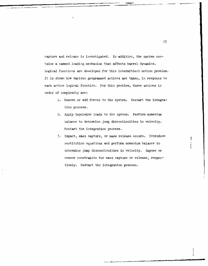
capture and release is investigated. In addition, the system con-
tains a cammed loading mechanism that affects barrel dynamics.
Logical functions are developed for this intermittent motion problem.
It is shown how various programmed actions are taken, in response to
each active logical function. For this problem, three actions in
order of complexity are:
1. Remove or add forces to the system. Restart the integra-
tion process.
2. Apply impulsive loads to the system. Perform momentum
balance to determine jump discontinuities in velocity.
Restart the integration process.
3. Impact, mass capture, or mass release occurs. Introduce
restitution equations and perform momentum balance to
determine jump discontinuities in velocity. Impose or
remove constraints for mass capture or release, respec-
tively. Restart the integration process.

16
CHAPTER 2
THE PLANAR RIGID BODY MODELING METHOD
FOR CONSTRAINED SYSTEMS
2.1 Introduction
The term "Rigid Body Systems" distinguishes the intent of the
analysis method and program developed in this chapter. Many of the
analysis programs existing today are based on the traditional notion
of "machines and mechanisms," in which the ideas of "links" and
"closed loop analysis" are embedded in the "geometry of mechanisms".
This limitation complicates an orderly approach to general constrained
dynamic system analysis.
Lagrange may have been the first to recognize the limitation
of the geometrical approach, as evidenced by the statement found in
the preface of his Mecanique Analytique [30]: "No diagrams will be
found in this work. The methods that I explain in it require neither
constructions nor geometrical or mechanical arguments, but only the
algebraic operations inherent to a regular uniform process. Those
who love Analysis will, with joy, see mechanics become a new branch
of it and will be grateful to me for thus having extended its field."
The concept of constraints in physical systems is not unlike
the concept of circuits in electrical systems. Kirchhoff stated
two basic laws that: (1 - voltage law) "The voltages with their

17
proper signs, taken completely around a mesh, add up to zero", and
(2 - current law) "The currents at a node, with due regard to
direction, add up to zero." From these laws and Ohm's law, two basic
methods of circuit solution have developed as follows:
(a) the mesh method of solution, characterized by the sum-
mation of voltages around meshes, is an application of
the voltage law.
(b) the nodal method, characterized by the summation of
currents at nodes, is an application of the current law.
Loop-closure methods of mechanism analysis are analogous to
the mesh method, (a). An alternate and more direct approach, first
developed on a large scale by Orlandea [10] for general three
dimensional analysis, is based on the nodal method, (b). He called
this method "the Node - Analogous Formulation" for mechanical systems,
derived by considering that D'Alembert's Principle for forces and
Kirchhoff's law for currents are analogous. He further identified a
finite number of standard components of mechanical systems (linkages).
While his method easily allows all of the constraints associated with
linkages, there need be no connotation of linkages in its development.
The analysis method presented here is developed according to
the nodal representation, as introduced by Orlandea. Since this
method is nearly devoid of geometrical and topological concepts, it
is adapted to a broad class of mechanical systems. These systems
may range from the most complex linkage mechanisms to articulated
tracked vehicles with electro-hydraulic control systems.

18
In this chapter, a general system of constrained equations of
rigid body planar motion is formulated. An implicit numerical inte-
gration method for automatically solving the system equations and
sparse matrix techniques are also discussed. Generalized coordinates
are defined to locate each individual rigid member of the system and
to express kinetic energy for each member. Constraints between
elements are taken as friction-free standard constraints, with pro-
visions for additional, non-standard constraint formulation, as
needed. In addition to standard constraints, springs, dampers, and
actuators connecting any pair of points on different bodies of the
system are included in the model. These standard force elements,
together with allowance for arbitrary non-standard forcing functions,
make the formulation quite general.
Implicit numerical integration and sparse matrix algorithms
[31, 32] were initially used in numerical integration of the
equations of motion. After considerable numerical experimentation,
it became apparent that implicit simultaneous solution of algebraic
and differential equations create artificially stiff [20] problems
and the integration of large systems of equations increases the
spectrum of frequencies with which integration algorithms must cope.
This prompted a search for new methods of solving the system equa-
tions of motion, which forms the basis of the method presented in
the following chapters. The implicit method is presented in this
chapter, for comparison purposes only. The basic constraint

19
formulation and equations of motion presented in this chapter are
used as the basis for developments in the following chapters.
2.2 Constrained Equations of Planar Motion
(a) Generalized Coordinates and Energy Equations
In order to determine the configuration or state of a planar
mechanical system, it is first necessary to define generalized
coordinates that specify the location of each body in the system. As
shown in-Fig. 2.1, let the x-y coordinate system be a fixed inertial
reference frame. Define a body-fixed . - fi coordinate system
embedded in a typical body i. The location of body i is specified
by the global coordinates (xi, yi) or the vector . of the origin of
its reference frame and the angle i of rotation of the body fixed
li-axis, relative to the global x-axis.
The center of mass of body i is located by a vector r inm.1
the body fixed coordinate system, with - components gM. and1
7M." In terms of the ger ralized coordinates x., Yi' and etp and the1
parameters m. and M. , the center of mass is located globally by1 1
X mi xi + gm. cos - m. sin Yi1 2.
mi = Yi + !m sin i+ nm. cos i (2.1)

20
p j
rx
y p~p
joints.

21
Thus, the kinetic energy of body i is
T12 + .2 (2.2)Mi\. rn.1 2. .
where m. is the mass of body i and J. is its centroidal polar moment1 2.
of inertia.
(b) Equations of Constraint
Figure 2.1 further depicts an adjacent body j, with body-
fixed coordinate system located by the vector .. Let arbitrary3
points pij on body i and pji on body j be located by vectors j-4
and r.., specified in the body fixed coordinate systems by coordi-
nates % ci. .i, and j... These points are in turn connected by
a vector r,
p 1 ij 3 j
The vector condition for a rotational joint between bodies i
and J, at points Pij and Pji' is simply r p yielding the follow-
ing pair of scaler constraint equations:
xi + ij cos 9, - ij sin 9, - xj - 9Ji cos p
+ ji sin cj =0

22
Yi + ij sin c0i + Tij cos y, yj -ji sin j
- Iji cospj= 0 (2.4)
If r in Fig. 2.1 is taken as a nonzero vector of fixed lengthP
rp a "massless link" of length rp connects points pij and Pjj" A
single scalar equation for this constraint can then be written as
4 2 2Ip I- r = +x i-1 1 x - " J cos cj11 p11- p =(x i + ij cos cpi - ij sin t i -x j CsY
+ 'ji sin yj)2 + (Yi + gij sin yi + Jij cosi
Y - 9ji sin 9 - T ji cos -2 _ r (2.5)
For a translational joint shown in Fig. 2.2, let points pil
and pi2 on body i, and points Pjl and pj2 on body j lie on some line
parallel to the path of relative motion between the two bodies, such
that the specified body fixed vectors and are of nonzero mag-
nitude. Since i and I are parallel, X. x - with zero z
component yielding the scalar equation
[(gi2 - 9.1) cos 'i - ( i2 - 'il) sin pi]
[( J2 - jl) sin cj + (Tj2 - ljl) cos

23
l ne of relative displacementbetween bodies
Pi2
I
0.
Figure 2.2. Rigid bodies connected by a translationaljoint.
Im n m m n n m n n nr n l • i /l / l I I I l n l

24
- [(J2 "jl ) Cos j - ijl ) sin Vj]
[ sin (p + ( - cos i= 0 (2.6)
Likewise, raji and are parallel, so ji × i yields a zero z
component and the second scalar equation
[x. + " cos n- ysni - xj il cos j+ i
(j2- 9jl ) sin cj + (ij 2 - cjl Cos tj]
- + l sin i+il cos cp. - YJ - !jl sin j - Tjl Cos C j
[(j2 " %jl) cos Yj - (TJ2 -'jl) sin Tj = 0 (2.7)
The parameters (gil' il ) and (1i2' i2 ) locate points Pil and pi2
in body i coordinate system, and (Cjl' mJl ) and (gj2' Tj2 ) locate
points Pjl and pJ2 in body j coordinate system.
Other constraints may be formulated by a similar process.
Denote by q = [ Y , y , T the vector of ganeralized coordinates
of body i and by q = [q , q , ... , q ] the composite vector of
all system generalized coordinates. In this notation, the holonomic
constraints of Equations 2.4 to 2.7 and other (perhaps time dependent)
holoiomic constraints can be written in vector function form as

25
(q,t) 0 (2.8)
where (q,t) = (qt), ..., Im(q,t)]T and the functions §V,
i = 1, ..., m, are assumed to be independent, i.e., the Jacobian
/aq E [M i/ q.] has full row rank.
(c) Equations of Springs, Dampersand Actuators
Internal forces due to other types of elements acting between
bodies may be obtained by a process similar to the constraint
equation development. For example, since springs, dampers, and
actuators shown in Fig. 2.3 generally appear together, they are
incorporated into a single set of equations. The equation for
spring-damper-actuator force is
=- + ck ()iJ + FO] ijsi (2.9)
where ij is the resultant force vector F 1 + Fy ij in thexij xij
1 -4element, s is the vector Iii cos Ce 1 + A ij sin a J between points
ij
s and s.., k.. is an elastic spring coefficient that may depend on
generalized coordinates and time, cij is a damping coefficient that
may depend on generalized coordinates and time, L0 is the undeformed
spring length, Iij is the deformed spring length, Iij is the time
derivative of Iii, and F0 is an actuator force applied along theij
element that may depend upon generalized coordinates and time. The
unit vectors and I are parallel to the x and y axes, respectively.

26
TS..
x
Figure 2.5. Rigid bodies connected by a spring-damper-actuator combination.

27
(d) Conservative and NonconservativeGeneralized Forces
Contributions of forces acting on body i to the system equa-
tions of motion are determined by employing a virtual work concept.
The virtual work of externally applied forces and spring-damper-
actuator forces acting on body i is written as
8 Q (qqt) 8x + Qy(q,q,t) 6y i + Q (qqjt) 8y. (2.10)Qx~ , xi y 8%
T1
The vector Qi [Qi Q1 , Q1] of generalized forces on body i isX defiT e 2 T n T
thus defined and Q = I , Q I is the vector of system
generalized forces. Typical generalized forces are calculated to
illustrate the procedure. Consider here the spring-damper-actuator
element of Fig. 2.3 where point sij on body i is located by the
vector . + r . A virtual change in the location of point s.. is
given by
( + = + r 8 + 3+ r 8y i
+P + r~ 8Ci(.1ay s ij i
Forming the dot product of i with 8 ( + determines contri-
butions to the generalized force expressions for body i as

28
iQx = FQ xij
Qi S F sin 9, -sj COS i )
'Ps x ij sij i
+ Fyi YU 9sii Cos (Pi" -s'j sin y i (2.12)
Generalized force contributions are summed for all externally and
ii
internally applied forces acting on body i, to arrive at Q.
(e) System Equations of Motion
Virtual displacements 8q that are consistent with constraints
(i.e., with time fixed) satisfy
q 8q = 0 (2.13)
where § q = /bq a [ati/aqj mx3n using subscript notation for dif-
ferentiation with respect to a vector.
The variational form of Lagrange's equations of motion, with
workless constraints, is [331
+(T) -T -QT 8q 0 (2.14)
dt q q
inenlyaple-ocsatigo -oyi to ariv atI-Q

29
which must hold for all 6q satisfying Equation 2.13. By Farkas'
Lemma [343, there exists a vector X E Rn of multipliers (called
Lagrange multipliers) such that
d T:T )TT
d (T) (T Q - jTq = 0 (2.15)q q q
which with Equation 2.8 form the constrained equations of motion of
the system. For planar systems treated here, Equations 2.1 and 2.2
yield
d (Ti)T _ (Ti)T M i (qi) qi A i (q.i i (2.16)dt A -(
q q
where
M4 0 - i + 761 cos i)
M,0 3-MiC soi in 4pn,)
si C o + 1 co + sin 9,) 1 2 +, 2
(2.17)
30
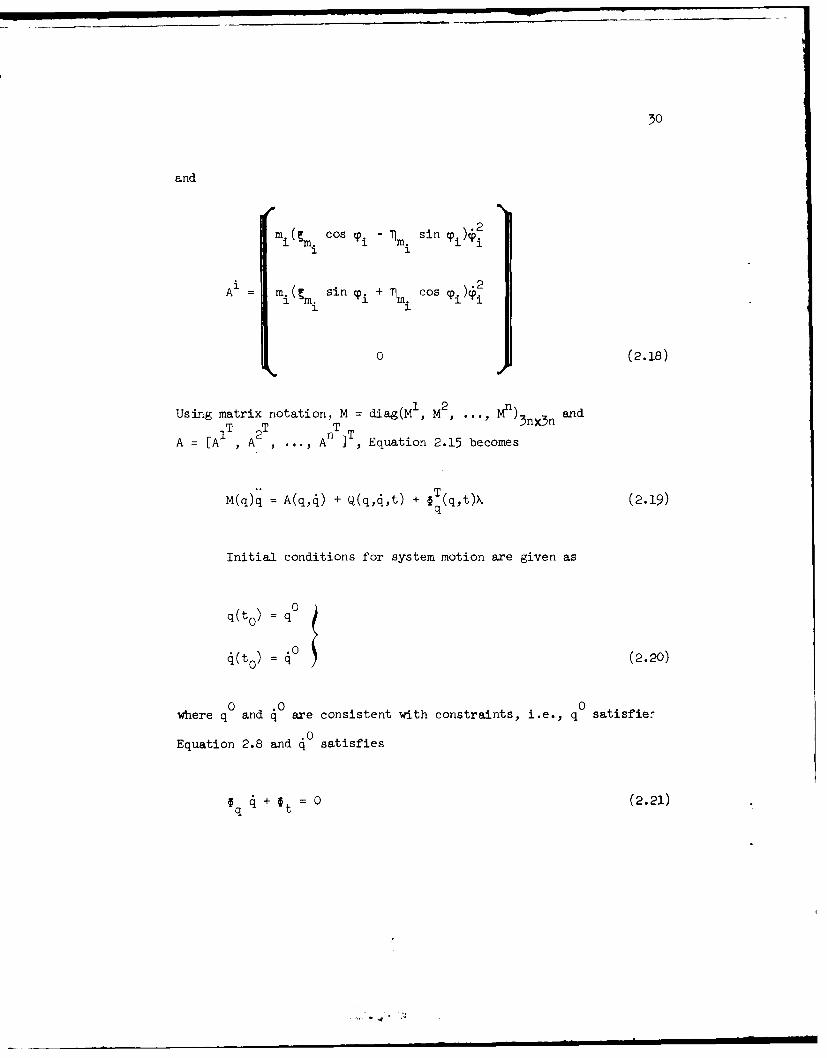
and
M. cos i - Tm sin ti)i.2
Ai = mi(, sin yi + 1 cos y, ) 2
1 2.
0 (2.18)
1 2Using matrix notation, M = diag(M , M, ... , M3n3 n and
JT ,-T T3nnA = [A , A , ... , A Equation 2.15 becomes
TM(q)q = A(q,j) + Q(q,j,t) + q (q,t)X (2.19)
Initial conditions for system motion are given as
q(t0) = q0
4(t 0 ) = q (2.20)
0 .0 0where q and q are consistent with constraints, i.e., q satisfier
Equation 2.8 and 0 satisfies
I q q + Ot = 0 (2.21)

31
2.3 Integration of Constrained Equationof Motion by an Implicit Method
(a) Numerical Solution of Algebraic and
Differential Equations
The method of numerically integrating differential equations
presented in this and following chapters requires that they be
reduced to first order form. This is accomplished by introducing
the vector
wzq (2.22)
into Equation 2.19 to obtain
M(q)*- A(q,w) - Q(q,w,t) T (qt)X 0 (2.23)q
with initial conditions
q(t0 ) = q0
W(t0 ) = q (2.24)
where
q(qO,t 0 ) w (t0 ) + t(qO,to) 0 (2.25)

32 1In order to solve the differential equations of motion,
numerical integration theory is used to obtain a set of approximations
that is suitable for digital computation. Integration of the equa-
tions of motion is accomplished as a simultaneous solution of
algebraic and differential equations. Standard approaches, however,
are designed to solve systems of differential equations of the form
= f(y,t) (2.26)
where y is an m-vector variable and f is an m-vector of functions.
A modified approach is taken here that allows for the simultaneous
solution of mixed algebraic and differential equations of the form
g(yt) = 0 (2.27)
where may not appear in some of the equations. Before introducing
the method to be used, it is instructive to review the standard
approach applied to solving Equation 2.26.
The basic method of constructing approximate solutions is to
place a grid of time points t., i = 1, ..., on the interval [0,T],
where h = t i+ - t is the grid spacing. One then approximates the
Lution y(t) of Equation 2.26 at the time grid points as yi 't Y(ti) "
The basic approximating equation for stiff differential
equations [35 and 36] is the Gear algorithm

3
n+l n4- ly-~
n- 0 n k n-j+l (2.28)
j=l
where the constants 0 and 0j, j=l,...,k, called Gear's coefficients,
are determined so that Equation 2.28 is exact for any polynomial
solution of Equation 2.26 of degree up to k. Gear's coefficients
[ 35 and 36] also have the property that the algorithm tends to be
stable, even for stiff differential equations; i.e., differential
equations with widely split eigenvalues.
A multistep formula that is used to solve Equation 2.27 is
derived from Equation 2.28. One progresses from tn to t n+1
solving Equation 2.28, together with
g(yn+l Y' n+l, tn+l ) = 0 (2.29)
Using the Newton formula to solve Equations 2.28 and 2.29, simul-
taneously, leads to
(in) Ay(in) + (m) .(m) 9(mn) (2.30)
(m). (m) g (m)m) gm
gy ay +g • y = -g(.0
where Ay(m) = y(mil) - y(m) and m represents the iteration number.
The time-step counter has been dropped here for notational simplicity.
Substitution of Equation 2.30 into Equation 2.28, noting that the
summation term of Equation 2.28 remains constant at each iteration,
yields the corrector formulas

34
k + 1j () _(i) (2.31)
A(m) _ 1 y(i) (2.32)
In the corrector formulas of Equation 2.31, the Jacobian
matrix J is defined as
1 = g(m) + g (mn) (2.33)
If Equation 2.27 is of the form -(y)k + f(y,t) = 0, which is
the case here, then Equation 2.31 is of the form
i lP (m) +P(m)(m) + f (m) A(m) g(m) (2.34)
The iterative corrector procedure is continued at each timestep until all of the Newton differences Ay (m ) ae below a specified
tolerance level. At each iteration, y and k are updated as
y(m+l) = y(m) + Ay(m)
k(m+l) = .(m) + &k(m) k (m) 1 Ay(m)
h 0

35
It is interesting to note that every element of # is obtained at each
time step, even though many elements of y may not appear in any of
the equations.
Since Gear's algorithm uses the Nordsieck vector representation,
the predicted Nordsieck vector at the present time step is obtained
by multiplying the Pascal triangle matrix times the Nordsieck vector
at the previous time step [35]. Details of convergence criteria,
error control, and procedures for this technique are discussed in
references 20, 35, and 36.
(b) Sparse Matrix Algebra
The system of nonlinear algebraic and differential equations
defined in the previous sections is loosely coupled. For two reasons,
however, no attempt is made to obtain a smaller system of equations
by reducing the number of equations through elimination of general-
ized coordinates. First, the Jacobian matrix formed by linearization
of the coupled equations and used in iterative solution by Newton's
method is sparse and can be very efficiently stored and decomposed.
Secondly, the repetitive nature of the loosely coupled equations re-
sults in compact and efficient computer routines for evaluating the
nonlinear equations and nonzero matrix entries. Recently developed
sparse matrix algorithms [37] make both of these operations prac-
tical and desirable. It has been shown [37] that is is usually
more efficient to solve large systems of sparse equations, rather
than smaller systems with a greater percentage of nonzero entries.

36
Consideration of matrix sparsity is important to the speed of
computation in problems of dynamic system analysis [351. When less
than 30 of the matrix entries are nonzero, it is inefficient to
store the matrix as a two-dimensional array. Instead, the nonzero
entries are stored in compacted form. The method most commonly used
for compacting the data is to store the row and column indices of
each nonzero-valued entry in the matrix in two vectors i and J, and
its value in a third vector A. This is called "i-J" ordering and is
a method of initially storing data from a user-supplied list of
physical system elements.
Sparse matrix algorithms are most efficient when the nonzero
matrix entries are stored in an organized manner. This usually im-
plies that they are evaluated row-by-row or column-by-column. The
previously mentioned repetitive matrix evaluation scheme is defeated
by this requirement, since it usually results in the evaluation of
small submatrices located at various positions throughout the matrix.
To overcome this difficulty, a special permutation vector is generated
from the row and column vectors describing the nonzero-valued posi-
tions. As each matrix entry is generated, it is directed to a
specific location in the "A" vector by a permutation index. At
completion of the matrix evaluation, all entries are stored exactly
as if they had been evaluated in column order. A sparse matrix
decomposition algorithm is then applied to the column-ordered matrix
and the standard LU factorization [551 is accomplished. Lull pivot-
ing is not achieved, but the algorithm chooses, among the acceptable

37
pivot elements, the pivot that results in a minimum number of fills
in the resulting L and U matrices. This is important for efficient
execution of the forward and backward substitution phases, since an
increased number of fills destroys the original matrix sparsity and
results in excessive computer time.

38
CHAPTER 3
KINEMATIC ANALYSIS AND GENERALIZED COORDINATE
PARTITIONING FOR DIMENSION REDUCTION IN
ANALYSIS OF CONSTRAINED RIGID BODY SYSTEMS
3.1 Introduction
The impliciL meth, d of simultaneously solving systems of differ-
ential and algebraic equations of motion described in Chapter 2 is
not desirable for sevci-al reasons. Implicit methods employ iterative
techniques requiring a Jacobian matrix of the combined system of
Equations 2.8, 2.22, and 2.23. For large systems, analytical expres-
sions for derivatives of Equation 2.23 are required if program
efficiency is to be achieved. Generalized forces, possibly discon-
tinuous, may be represented by digitized data, from which it is
difficult or impossible to provide derivatives, either analytically
or numerically.
In the implicit method, the coordinates q, velocities w, and
Lagrange multipliers X of Equations 2.22 and 2.23 are treated as
state variables, which are determined iteratively by the integration
algorithm. The algorithm obtains q and w by integration, allowing
it to maintain error control and accurate prediction of these vari-
ables. The algorithm uses the same predictor for Lagrange multipliers.
Since generalized forces may be highly irregular or discontinuous,

39
irregular and discontinuous joint reaction forces are reflected in
f i, lafranre multipliers. The net result is a poor prediction of
Lagrange multipliers, requiring more iterations to achieve conver-
gence (or quite often divergence) in the corrector step. A reduction
in time stepsize is then required to achieve better predicted values.
Stepsize reduction in the implicit algorithm is undesirable
since it requires more computer time and often leads to failure of
the algorithm to achieve a solution, even when extended precision
computer arithmetic is used. The reason for corrector divergence is
as follows: The time step h appears in the denominator of the(min Euto .3 n shgt
expression multiplying the term gy in Equation 2.3, and as h gets
smaller, these terms get larger and dominate the Jacobian matrix.
The Jacobian matrix may thus become badly conditioned or singular.
A badly conditioned matrix results in erroneous Newton differences
associated with Lagrange multipliers, leading to divergence of the
corrector.
The numerical method developed in the following chapters offers
significant improvement over the implicit method of Chapter 2.
Iterations are limited to the solution of constraint equations, thus
requiring a much smaller Jacobian matrix. Since iteration only
involves predicted variables with error control, convergence is much
faster. In fact, the iteration step is frequently bypassed, because
the constraint equations are satisfied by the predicted variables.
Badly conditioned matrices, as described earlier, are avoided and
single precision computer arithmetic can be used.

4o
Another advantage of the proposed method is that a minimal set
of differential equations is identified by the program and solved by
an explicit integration method. This avoids a Jacobian matrix
involving derivatives of generalized forces.
3.2 System Constraints
(a) Classification of System Coordinates
The ultimate goal of this research is to develop analysis
techniques that use system constraints to improve numerical effi-
ciency and accuracy, while at the same time reducing the preprocessing
requirements of the user. To this end, an understanding of what
constitutes a constraint is essential. According to Webster [38] a
constraint is confinement; restriction; force; compulsion; or
coercion. In the tradition of mechanics, a constraint is any condi-
tion that reduces the freedom of a system. Another notion is
"something that limits motion".
In the development of Chapter 2, a system was assumed to be
composed of n rigid bodies in a plane, each with three degrees of
freedom. Algebraic constraint equations were also formulated and
reaction forces at the constraint surfaces were introduced into the
system differential equations of motion, through a vector of Lagrange
multipliers. The equations of motion and constraint equations were
solved iteratively and no account was taken of the number of system
degrees of freedom. Mathematically, this system has 3n degrees of

41
freedom and the algebraic constraints/constraint reaction force
system represents a restriction on admissible movements.
The formulation of Chapter 2 treats every coordinate as inde-
pendent, hence the system has 3n generalized coordinates. A
formulation reduces the number of degrees of freedom when the alge-
braic constraints/constraint reaction force balance is used to
eliminate generalized coordinates from the system equations of motion.
Application of constraint relations to mathematically reduce the
number of degrees of freedom introduces a new problem of identifying
independent and dependent variables. If constraint equations mathe-
matically eliminate r degrees of freedom, there are (3n-r) independent
generalized coordinates and the remaining r coordinates become
dependent position coordinates. For notational purposes, let the
symbol u designate dependent variables and let v designate independent
T T Tgeneralized coordinates. With this notation, q = [u , v I .
Partitioning of q into u and v must be done in a manner that
does not degrade program efficiency or increase numerical errors. If
the partitioning were done on a random basis, there are 3n'/r!(3n-r)!
possible combinations, most of which would be mathematically unaccept-
able. Wells [393 stated, when discussing the selection of
independent coordinates for simple problems: "It is a well known
fact that certain coordinates may be more suitable than others.
Hence the quantities chosen in any particular case are those which
g ill Il

42
appear to be the most advantageous for the problem in hand. The final
choice depends largely on insight and experience." This approach is
also taken in another well developed and documented planar rigid body
modelling program [13]. However, in this case, steps are taken to
circumvent some of the numerical difficulties associated with bad
choices of independent variables. When systems become large and
complex, geometrical insight and experience quite often fail and
mathematical techniques must be employed.
To the author's knowledge, the first organized method for
selection of a good, and possibly best, set of independent generalized
coordinates for large scale systems was developed by Sheth [40, 16].
Although he does not prove that the selected set is best, he does
provide numerous arguments, based on geometrical considerations and
example test problems, that indicate the set has desirable features
of a properly driven kinematic mechanism. This approach has sound
mathematical appeal and will be developed as the tool for efficient
dimension reduction of constrained systems.
(b) Iterative Solution of SystemConstraint Equations
The system constraint equations developed in Chapter 2 are
written symbolically in the form
O(q,t) = 0 (3.1)

43
where all equations may not be independent, but they are consistent.
That is, the Jacobian matrix q with m rows and 3n columns has row
rank 0 : r g m and r ! 3n. There are one or more nonsingular sub-
matrices of q of rank r. Gauss-Jordan reduction of the matrix Iq)
T T Twith double pivoting, defines a partitioning of q = [u , v ] such
that §u is a submatrix of q of rank r, whose columns correspond to
elements u of q, and Iv is a submatrix of §q whose columns correspond
to elements v of q. Furthermore, the matrix §u has ideal numerical
properties associated with double pivoting.
The subprogram described in Appendix A determines the rank of '
q and its linearly independent rows and columns. It performs
Gaussian elimination with row and column permutations that bring
independent rows and columns to the top and left of the matrix, until
the remaining submatrix in the lower-right corner is null (all of its
elements are less than some specified tolerance). In addition, the
matrix is decomposed into factors of the form
- and - I -LR 0 0 , 0
which are superimposed onto the original matrix. The factor products
L. U L I UR
represent, in permuted form, the original matrix 0 ; specifically,
L.U = @u and L.UR = *v" The columns of U and UR determine a

permutation of q into dependent (u) and independent (v) variables,
respectively. The rows of L and LR determine a permutation of con-
straint equations § = 0 into independent 1 and dependent §2 equations,
respectively. In addition, the respective lower and upper triangular
matrices L and U are nonsingular.
In the following chapters it is often convenient, for clarity,
to express matrix equations in the above permuted and factored forms,
rather than in terms of the original matrix §q'
Some additional comments can be made concerning the matrix §q
and its corresponding submatrices. First of all, 0q may be null.
That is, there may be no constraints in the system, in which case
v = q and u is null. This special case requires no further analysis
and need not be considered here.
If 0v is null there are no independent generalized coordinates
and u = q. In this case, in view of Equation 3.1, the system is
either a structure @ = O(q) or its geometry is completely determined
as a function of time, § = (qt).
If roots of Equation 3.1 are to be found, an iterative procedure
such as Newton's method is required. With an initial estimate q(O)
of the system configuration at time to, the matrix q(q(O),to) is
evaluated. The iterative equation is then
Oq[q(j),t 0] [q(j+l) - q(j)] = - §[q(J),to], J = 0,1,... (3.2)

45
where j is an iteration counter. The solution of Equation 3.1
requires the determination of q(j+l) in Equation 3.2. If Equation
3.1 is consistent, there is at least one solution. If the rank is
less than 3n there are an infinite number of solutions.
Assume that the matrix has been decomposed by the subprogram
described in Appendix A. Equation 3.2 may then be written in per-
muted form, in terms of the previously mentioned matrix factors and
partitioning, as
L U [u(j+1) - u(j)] + L . uR [v(j+l) -v(j)]
[q(j),t O] (3.3)
IF U [u(j+l) - u(j)I + I • U - [v(j+l) - v(j)J
2 q(j),t0 ]
Noting that v are independent generalized coordinates, one may set
v(j +l) = v(j) and Equation 3.3 reduces to
L U . [u(j+1) - u(j)] = - 1 (3.5)
Since matrices L and U are nonsingular and triangular, simple
forward elimination and back substitution determines u(j +1).
Equation 3.4 is not required in the intermediate steps of
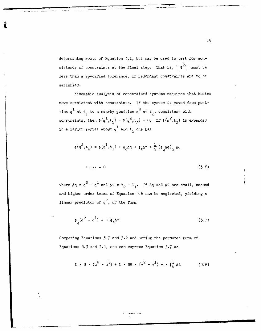
46
determining roots of Equation 3.1, but may be used to test for con-
sistency of constraints at the final step. That is, 1 f21l must be
less than a specified tolerance, if redundant constraints are to be
satisfied.
Kinematic analysis of constrained systems requires that bodies
move consistent with constraints. If the system is moved from posi-
tion qI at tI to a nearby position q2 at t2, consistent with
constraints, then i(q1 t1 ) = §(q2,t2 ) = 0. If (q2 ,t2 ) is expanded
in a Taylor series about q and t one has
§(q2,t2= I(ql,tl) + t qAq + 1
+ . 0 (3.6)
where Aq = q - q1 and At =t 2 - t I . If Aq and At are small, second
and higher order terms of Equation 3.6 can be neglected, yielding a
2linear predictor of q , of the form
Sq(q 2 ql) = - 0tAt (3.7)
Comparing Equations 3.7 and 3.2 and noting the permuted form of
Equations 3.3 and 3.4, one can express Equation 3.7 as
L - (u2 - u1) + L •UR (v2 - v) = - 1 At (3.8)

47
LR •U (u2 -u1 ) + LF • U (v - v) =- t At (3.9)
Since L and U are nonsingular and with v2 and t2 specified, Equation
23.8 determines u . It is most efficient to solve Equation 3.8 in two
steps, since the matrix product L • UR is not calculated by the sub-
program. First, solve
L U - i At (3.10)t
by forward elimination and back substitution and then use the pre-
calculated matrix H to obtain
2 1 2u1 *
u -u =H.(v2 v) +u (3.11)
Equation 3.3 is then used to iteratively correct u2, to satisfy
Equation 3.1.
The matrix product L • UR of Equation 3.8 is never evaluated,
since the matrix
H U-1 . L-1 . L , UR = U-1 UI
is required in Equation 3.1. In fact all subsequent equations in-
volving the matrix L • UR ultimately require the matrix H for
solution, so for convenience, H is calculated and stored in the space
riginally occupied by UR.
I

48
To avoid excessive corrector iterations, it is desirable that
Equation 3.1 predict u 2 with small error. Since Aq was assumed small
and Av is fixed, Au should be small. Gaussian elimination, using
full row and column pivoting to partition q into u and v, accomplishes
this. Equation 3.1 may be written simply as
Au = H Av + u
As noted in Appendix A, the largest matrix element is permuted to the
diagonal position at each intermediate step, when performing Gaussian
elimination with full row and column pivoting. This process tends to
maximize the magnitude of diagonal elements of U and to minimize the
-1magnitude of elements of UP. Noting that H = - U . UR, one would
expect that the magnitude of elements in H will be substantially less
than 1 and that the magnitude of elements in Au will be substantially
less than the magnitude of elements in Av.
This argument could be strengthened if a reliable estimate for
the condition number of U, cond(U), were available. In general,
Gaussian elimination with full row and column pivoting yields well
conditioned matrices [41]. However, one can find examples in which
it does not. If cond(U) and the norm of U are known, the norm of
-l isU Is
I Il = ond(U)/I Ilul(l12

49
The norm of U is, by construction, large since the largest elements of
0q were permuted into it. If cond(U) is small (on the order of 1),
then by Equation 3.12, lU-11 I i/I lul I.
Since the elements of U dominate those in UR, it is reasonable
to expect that 1IIUI >> I URII and JIU-111 I IURII << 1, by the
assumption of a well conditioned U matrix. Finally,
IIHII = II- U -1 URII < IIU- 1 II IIJURII << 1, supports the contention
that 1 IAqj is reduced by proper selection of u and v.
3.3 Kinematic Velocity andAcceleration Analysis
(a) Velocity Analysis
For kinematic analysis, if one specifies independent general-
ized coordinates as functions of time, independent velocities and
accelerations can also be expressed as functions of time.
The remaining dependent velocities and accelerations can then
be determined by differentiating the constraint equations with respect
to time. Differentiating Equation 3.1 with respect to time yields
q j + t 0 (3.13)
Comparing Equations 3.13 and 3.2, equations similar to Equations 3.3
and 3.4 can be expressed as
L U + • = - 1 (3.14)
nmu

50
E U + L 2 (3.15)
The solution of Equation 3.14 determines i and Equation 3.15 is auto-
matically satisfied by the consistency requirement of Equation 3.4.
Similar to the method of solving Equation 3.8, first solve
L . *= - 1 (3.16)
by forward elimination and back substitution and then use the pre-
calculated matrix H to obtain
= H - + a* (3.17)
Inspection of Equation 3.17 reveals that the matrix H relates
dependent velocities to independent velocities and this matrix is
generally referred to as an influence coefficient matrix. From a
geometrical point of view, a properly driven mechanical system is one
in which the ratios of output to input velocities are minimized
[40, 16] . In addition, the system is driven with the greatest
mechanical advantage.
Recall that the method of decomposing § determined H, suchqI
that Au was reduced in Equation 3.11, hence i is also reduced in
Equation 3.17. A further advantage of minimizing velocity ratios is
that errors in independent velocities are not amplified when calcu-
lating dependent velocities. This will be important when solving the
system differential equations of motion in Chapter 4.

51
(b) Acceleration Analysis
Having determined all system position and velocity variables,
one may proceed to determine dependent accelerations. Equation 3.13
may be differentiated with respect to time to obtain
q q ( )qq q + 2 qtq + =tt 0 (3.18)
For convenience, denote the three known terms in Equation 3.18
as
C(q,j,t) = (0qd)q j + 2 qt4 + tt (3.19)
and partition Equation 3.18 as
L • U • U + L U • = - C1 (3.20)
LR • U • U + LR ' UR = - C2 (3.21)
The independent generalized accelerations V are presumed known, so
Equation 3.20 determines U and Equation 3.21 is automatically satis-
fied by the consistency requirement of Equation 3.4.
Similar to Equation 3.8, Equation 3.20 is solved in two steps
L " U = - (3.22)

52
by forward elimination and back substitution. Also,
U =H (3.23)
where the precalculated influence coefficient matrix H is used. Note
that errors in independent generalized accelerations V are reduced,
in calculating the dependent accelerations U, because of the small
norm of H.
3.4 Kinetostatics of
Constrained Systems
The analysis method of Section 3.2 allows one to identify an
ideal set of independent generalized coordinates, from which to drive
an arbitrary, constrained multiple-degree-of-freedom system. Kineto-
static analysis may then be applied, using the method of Section 3.3,
to determine all forces in the system, including inertial forces,
generalized joint reaction forces, and the generalized driving forces
required to achieve the specified system dynamics. One could then
envision the same system reacting to this set of generalized driving
forces. In this case, a system of differential equations of motion,
solved by the methods of Chapter 4 will determine the same dynamic
response. The first system is displacement driven, requiring speci-
fied generalized coordinates, and the second system is force driven,
requiring specified generalized forces. The two examples demonstrate
a duality between specified generalized coordinates and specified
generalized forces.

53
Using the permutations of the previous sections, equations of
motion for constrained systems derived in Chapter 2 may be partitioned
into
UT • T I +UT •LT • 2 uu Mtf+MuvU L 1X +J LR T.x =M u ~+M
- (Au + Qu) (3.24)
T T 1 T T 2 -UR LT .X + UR . LR /J = MVU + Mv
- (Av + Qv) (3.25)
Lagrange multipliers X and X2 are associated with independent con-
1straint equations § = 0 and redundant or dependent constraint
equations 2, respectively. The multipliers X 2 are not determined by
Equations 3.24 and 3.25, but must be obtained from other methods,
such as local body deformation models that specify relations between
1 2X and 2
Let
Fu=u L x1+ RT 2 (3.26)
and
Fv = RT L T x1+U TQ .*R T x 2 (3-27)
r. 2U,.ZN~....'

54
Then, by combining Equations 3.26 and 3.27 with H = - U UR, it is
easy to show that
Fv = HT F1 (3.28)
1 2holds for any value of X and X . Assuming that redundant constraints
are consistent, they can be eliminated without effecting the system
dynamics, which is then equivalent to setting X 2 to zero in Equations
3.24 and 3.25.
A displacement driven system with specified generalized coor-
dinates has corresponding unknown generalized forces. In this case,
let the generalized force vector Qv be composed of known Qv* and
unknown Rv forces
v V* v (329)= Q + R(-9
Generalized constraint reaction forces become
Fu = 1T LT . X = Muu + MuvV - (Au + Qu) (3.30)
and the unknown generalized driving forces become
Rv = Mv"U + Mv - (Av + Qv*) + HTFu (3.31)

55
It is not necessary to evaluate X to determine the generalized con-
straint reaction forces.
Equations 3.30 and 3.31 may be made more tractable by substi-
tuting Equation 3.23 to eliminate dependent accelerations, thus
F1 = (MUUH + MUV - (Au + QU - MU'.) (3.32)
Rv = (MvuH + Mw)V - (Av + Qv* - Mvu*) + HTF u (3.33)
If forces Fu are not desired, one may combine Equations 3.32 and 3.33
to eliminate F u , obtaining
RV = [MW + MVH + HT(Muv + MuH)jV - (Av + QV* - Mv"U*)
SHTu + Qu _ MU (3.34)
Equation 3.34 thus relates generalized driving forces Rv to specified
generalized coordinates v, where velocities and accelerations are
assumed known.
The kinetostatics problem with full consideration of all
forces in the system may now be solved. The basic steps are, pre-
suming equations and initial coordinate estimates have been given:
Step 1. Identify dependent and independent variables.
Decompose the matrix I q. using the method of Appendix A, to determine
a partitioning of q into u and v.
- ~ -- - O

56
Step 2. Solve the constraint equations. Specify v and iter-
atively solve Equation 3.1, using Equation 3.5. Check consistency of
2equations I = 0.
Step 3. Calculate system velocities. Specify -r and determine
-d from Equations 3.16 and 3.17.
Step 4. Calculate system accelerations. Specify V, evaluate
C , and determine U from Equations 3.22 and 3.23. Dependent acceler-
ations U are not required if Equations 3.32, 3.33, or 3.34 are used
in Step 5.
SteP 5. Determine generalized constraint reaction forces Fu
and system driving forces Rv. Evaluate A and Q and determine Fu from
Equation 3.32 and Rv from Equation 3.33 or Equation 3.34. Individual
constraint reaction forces are obtained by first solving
UTLT 1 = Fu
(obtained from Equation 3.26 with X' = 0) for X 1 . Note that
Fu = T lu
and
F v =Tilv

57
Each colunmn entry in a given row of T (fT) times the corresponding
row entry of KI determines the generalized constraint reaction force
contribution to the generalized coordinate associated with the given
row of 0T ( T) . Hence, one may calculate reaction forces at any con-
straint in the system.
3.5 Sparse Matrix Considerations
As noted in Chapter 2 the nodal method of constraint formula-
tion yields loosely coupled equations with a corresponding sparse
Jacobian matrix. If the system has a large number of constraints,
sparse matrix manipulation algorithms will be efficient. While the
equations derived in previous sections still apply, they may be
expressed in different forms to avoid unnecessary calculation of
sparse matrix products.
Sparse matrix algorithms that factor matrices are not suitable
for determining the partitioning of coordinates q into u and v. They
employ a partial pivoting strategy and to maintain efficiency, usually
do not select the largest pivotal elements. The matrix u so identi-
fied will have a smaller norm than the corresponding matrix identified
by full pivoting. The corresponding matrix H = - f -lv will thenu v
have a larger norm. Therefore, Gaussian elimination with full pivot-
ing is periodically applied to the full matrix representation of q
solely for the purpose of determining the ordering of q into u and v.
Once established, a matrix I is appended to q to form a modified
matrix T of rank 3n such that when q is permuted, corresponding to
q qi e I

58
the permutation of q into u and Iv it is of the formq u
_ I V
where I is an identity matrix. The matrix I is readily constructed
from the permutation vectors generated by 'he algorithm described in
Appendix A.
An algorithm employing sparse matrix techniques for a dis-
placement driven system with full consideration of inertial and
externally applied loads is given in the following steps:
Step 1. Periodically identify dependent and independent
variables by decomposing the matrix §q, using the method of Appendix
A. Construct the matrix 0q by appending the matrix I to 0q'
Step 2. If a first order prediction of dependent variables
(u ) to an adjacent position (u 2 ) is desired, append to Equation 3.7,
*q Aq I t At
the equation
2 1AV =vV -V
which in matrix form becomes
t At 1
SqAq v 2 -v (3.35)

59
The matrix q of rank r = 3n is then factored by sparse matrixq
algorithms and Aq is determined by Equation 3.35.
S . The predicted dependent variables u are now corrected
iteratively until the constraint equations are satisfied by appending
to Equation 3.2,
1 Aq = -q
the requirement that independent variables remain fixed
AV= 0
which in matrix form becomes
qAq=[ ] (3.36)
Dependent variables are iteratively corrected until the independent
constrinats are satisfied and any dependent constraint equations are
then checked for consistency.
Step 4. Analysis of displacement driven systems requires that
independent velocities be specified. Denoting these as v , write
Equation 3.13 as
q q = -t

60
and append the equations
v= vS
which in matrix form becomes
Si= (3.37)
Equation 3.37 then determines q.
Step 5. Combine Equation 3.18 and 4 = Vs to form the matrix
equation
q ] = (3.38)
where C (q, , t) is given by Equation 3.19. Solve for accelerations
SteP 6. Using Equation 2.23 and noting from Equation 3.29
that unknown generalized forces Rv associated with independent
generalized coordinates must be determined, one has
q v
which in matrix form becomes
1 T v = M- (A + Q) (7 *9)

61
As noted in Section 5.4, Lagrange multipliers corresponding to
redundant constraints, arc not; determined by Equation 5.39. However,
if redundant constraints are consistent, their corresponding multi-
pliers can be set to zero. The remaining multipliers and unknown
forces Rv are then determined by Equation 3.39 and all forces in the
system are determined.
Equations 3.35 to 3.39 employ the same sparse matrix q orq
q, thus only one matrix factorization is required for each execution
of steps 2 to 6. Matrix and vector products are also indicated for
evaluation of the right hand side of Equations 3.38 and 3.39. How-
ever, these matrices are very sparse and analytical expressions are
written directly for the indicated products requiring no additional
matrix manipulation.
To maintain program efficiency the full matrix decomposition
of Step 1 should not be performed too frequently, yet often enough
to avoid numerical problems associated with nearly singular 0u
matrices. Available methods for monitoring the condition number of
Ou require more time than is required for its original determination.
Monitoring velocity ratios, however, may be an inexpensive, though
not entirely reliable, technique for determining the need for a new
matrix. Equation 5.15 may be partitioned and written as
-I
U v t ~Rnn

62
To approximate the amplifying ability of 1-1 one could evaluate the
number
t
following the initial determination of u, (i = 0) and at each
successive application of the sparse matrix code (i > 0). When the
estimate of increase in matrix norm K i/K0 exceeds a specified level,
a need for a new partitioning of q is then indicated.q
II

63
CHAPTER 4
CONSTRAINED EQUILIBRIUM AND DYNAMIC ANALYSIS
4.1 Introduction
In Chapter 3, differential equations of motion are developed
for a general constrained planar rigid body system. It was demon-
strated that the complete system state is determined when all
independent generalized coordinates, velocities, and acclerations
are specific functions of time. These equations, however, must be
numerically integrated when independent variables are allowed to move
under the influence of applied force. Therefore, this chapter is
devoted to development of an efficient numerical integration
algorithm utilizing kinematic properties of constraints to obtain
a minimal system of differential equations of motion.
Efficiency is achieved by minimizing the number of differential
equations to be solved, which improves numerical integration perfor-
mance. Paul [ 42 ] has indicated that the minimum number of first
order differential equations formulated by any of the existing
general purpose programs is 2 dof (degree of freedom). Only 2 dof
first order equations are required by the method described in this
chapter.

64
4.2 Equilibrium Analysis
Transient, dynamic analysis of complex constrained mechanical
systems is often initiated from a position of partial or complete
equilibrium. Static equilibrium analysis is often required prior to
initiation of transient analysis of vehicular systems, because the
nonlinear characteristics of suspension elements make it difficult
to estimate equilibrium configurations. Partial equilibrium analysis
is required when one or more of the bodies in a system have no
equilibrium position or when internal forcing elements such as springs,
are to be given initial lengths differing from their equilibrium
lengths. In this case, temporary constraints are placed on or
between bodies prior to equilibrium analysis and released prior to
transient analysis.
Various methods may be employed to solve equilibrium equations.
Since they are highly nonlinear, iterative techniques are required.
One iterative technique that is often employed is Newton's method
for finding roots of nonlinear algebraic equations. Newton's method
may converge to unstable equilibrium configurations, or diverge, if
poor initial estimates of configuration are given. However, it is
easy to implement and has been used to find equilibrium of systems
with many degrees of freedom.
The implicit numerical integration method for transient
analysis of Chapter 2 requires the Jacobian matrix of the equations
of motion for solution of Equation 2.23. Noting that velocities and

65
accelerations are zero for static equilibrium, Equation 2.23 expresses
equilibrium equations as
T (q, to) X + Q(q, to) = 0q 0 0
(4.1)
(q, t) = 00
and the corresponding matrix iterative equation is
T T Aq(j)Tq q q q
- -(4.2)
q0 AX(j)
This method, requiring the simultaneous determination of q
and X, is undesirable because it involves the repetitive solution of
a large system of equations and a reasonable estimate of the vector
% must be given, since it appears in the matrix. Poor estimates of
X may lead to a badly conditioned or singular matrix in Equation 4.2
and divergence of Newton's method. For this reason, iterative
techniques that do not involve Lagrange multipliers are desirable.
In Chapter 3 a method for identifying the independent gener-
alized coordinate vector v was developed and a reduced system of
differential equations of motion, Equation 3.34, was derived. Noting

66
that velocities and accelerations are zero for static equilibrium,
Equation 3.514 yields
R - H(q, t 0 )T Q(q, to)U - Q(q, t (4.3)
where
t(q, t 0 ) 0 (4.4)
The forces R must be applied to the independent or specified
coordinates vs in a displacement driven system. In an equilibrium
situation the variables v are free and the forces Rv must be zero.
A condition for static equilibrium is then
R 0 (4.5)
Equations 4.4 and 4.5 may be solved iteratively, by noting that
Rv = RV(u, v). Therefore, with du = Hdv, the iterative equation
dR v AV == .p (14.6)dv v u
determines the solution of Equation 4.5. The matrix in Equation 4.6
is evaluated by numerical differencing, because 1) the matrix H and

67
,reneralized forces appear in Equation 4.3, 2) analytiral expressions
for their partial derivatives are difficult to obtain, and 3) the
derivatives are not required for subsequent transient analysis.
4.3 Initial Conditions
Obtaining suitable initial conditions for transient analysis
poses problems when constrained mechanical systems have many degrees
of freedom. Often one desires to specify initial conditions on
various coordinates and their first derivatives or initial conditions
on first derivatives of other coordinates. The independent variable
set identified by factoring the constraint Jacobian matrix may not
agree with the above selected variables so some initial conditions
would be changed when satisfying constraints. The method described in
Section 3.6 allows one to hold selected coordinates and velocities at
their specified values by appending temporary constraints. The only
requirement is that these constraints be consistent with other con-
straints. This method is employed below. The following seven steps
outline an algorithm for achieving suitable initial conditions, from
a starting configuration that is consistent with constraints or from
a partial or lull equilibrium configuration:0
Step 1. Specify an initial estimate q of the constrained
system configuration. This estimate must be near the expected final
configuration to insure convergence. If static equilibrium is to be
obtained, the estimate must be near the desired equilibrium

68
configuration to avoid convergence to alternate stable or unstable
0configurations, or divergence. Set q = q
Step 2. If some elements of q are to remain fixed during
initial assembly of the constrained system or during static equilib-
rium, for example in partial equilibrium, append to Equation 4.40
additional algebraic constraints of the form q, - qj 0= , where j
identifies the variables to be held fixed. Other types of algebraic
relations between coordinates can also be formulated as needed. These
constraints will be removed prior to step 6.
Steo 3. Evaluate the modified constraint matrix *q (including
constraints of step 2) and factor, as described in Appendix A, to
determine a submatrix I u of maximal rank and to determine a partition-
ing of q into u and v (dependent and independent coordinates,
respectively). If q does not have full row rank, then too manyq
constraints or inconsistent constraints are specified. Therefore
some equations are dependent and they can be temporarily ignored in
the iterative procedure of Step 4.
Step 4. Keeping the independent variables v fixed, iterate
with Equation 3.5 to solve the independent constraint equations of
step 2, until 1)§11 < E, where E is a specified closure tolerance
level. If there are dependent constraint equations, check them for
violation. When dependent constraints are violated, inconsistent
constraint conditions have been specified and a meaningless solution
may result. If static equilibrium is not desired, go to step 6.

69
Step 5. Determine a new estimate for v from Equation 4.6 that
reduces UIRvJJ. if lpRvfl >6, a specified force unbalance tolerance,
return to step 3. If the iteration in steps 3 to 5 diverges, either
inconsistent constraints have been imposed or initial estimates of
system configuration are in error.
.0Step 6. Specify initial estimates for velocities q and set
.00= . The velocities 4 are adjusted to satisfy Equation 3.13,
0evaluated at q from the above steps. If some elements of i are to
.0remain fixed at q0 , append to Equation 3.13 additional equations of
.0the form k 0 k 0, where k identifies the variables to be held
fixed. Other types of relations between velocities can also be form-
ulated as needed. These constraints will be removed prior to step 1
of transient analysis.
Step 7. Factor the modified matrix of Equation 3.13 as
described in Appe,dix A, to determine a partitioning of 4 into i and
v (not necessarily the same partitioning as in step 3). Calculate
using the above partitioning in Equations 3.16 and 3.17. If the
above matrix lacks full -ow rank, some equations are dependent and
must be checked for consistency. If dependent equations are not
satisfied, inconsistent constraints on velocity are specified and a
meaningless solution may result. Otherwise, a consistent set of
initial conditions is now available for transient analysis.
4.4 Numerical Integration of the
Equations of Motion
The reduced system of differential equations of motion,
derived in Chapter 3, were expressed in the form
*,w~m~m nmm~~m -- '-

70
Rv =[M7 + M7 H + H'(Muv + M u H) N- (Av +Q -M U*)
_ HT(AU +QU Muu u*) (47)
Noting that the independent variables v are free, the driving forces
Rv are zero in Equation 4.7. Therefore Equation 4.7 can be written
as
[M + HTMUV + (M + HTMU)H]V = Av + Q + HT(A +Qu)
(vu + HTuu) (4.8)
In order to integrate Equation 4.8, it is helpful to write it
in first order form. To do this, define the vector s of independL Ivelocities as
= s (4.9)
and write the total vector 4 of generalized velocities in terms of
s, using Equations 3.16 and 3.17, as
v~) +(s u (4.10)
where L • U • u - • With this notation Equation 3.19 becomes a
function of w,
.4.

71
= qw + 2 qt w+
Equation 5.22 is used to evaluate u , and Equation 4.8 becomes
[M' + HTMuv + (MVU + HTMuu)HA = AV + QV + HT(Au + Qu)
(Mv u + HTMuu){ (4.11)
Decomposing the above mass matrix as described in Appendix A, one
may solve Equation 4.11 for . Equations 4.9 and 4.11 now form a
system of 6n - 2r = 2 dof first order ordinary differential equations
where n is the number of bodies in the system and r is the number of
dependent variables in u.
The selection of numerical integration algorithms for dynamic
analysis should be based on the type of differential equations to be
solved. Since most mechanical systems are non-stiff, an explicit/
implicit-predictor/corrector method may be employed [ 28 ]. Pre-
dictor/corrector algorithms require fewer function evaluations than
Punga-Kutta methods and allow interpolation between solutions with no
additional function evaluations. This is important, since the com-
putational overhead in evaluating the reduced system of differential
equations is significant. The explicit/implicit-predictor/corrector
algorithm DE/STEP, INTRP [ 28 ] is used, since it is well developed
and easy to adapt to the equation requirements. In addition, the

72
integration algorithm DE estimates relative stiffness and terminates
execution if the system becomes too stiff.
A numerical integration algorithm based on the development in
previous sections and the explicit integration method is now pre-
sented. The following steps outline the numerical integration
algorithm.
Let i, initially 0, be an indicator for the current time step;
i.e., i = 0 implies t = t . Steps 1 to 5 are satisfied when start-
ing, from results of the preceding algorithm, so start with step 6.
SteP 1. Check HjiIj < c. If satisfied, the extrapolated
dependent variables u are satisfactory, therefore go to step 4.
A polynomial extrapolator is maintained for u by the integra-
tion algorithm at little additional overhead. The term extrapolator
is used rather than predictor, because the program does not maintain
full error control on the variables u. Since this extrapolator may
be of any order up to 12, the constraints (u, v, t) will usually
satisfy the above closure test, thus avoiding the following steps 2
and 3. In addition the partitioning of q into sets u and v depends
upon q and t because q is a function of q and t. Since the extra-
polator for u and the predictor for v have the same form, it is not
necessary to interrupt the integration process to account for dif-
ferent sets u and v. Error control within the integration algorithm
is maintained only on v since steps 1 to 3 are equivalent to main-
taining error control on u.
73
Step 2. Evaluate q and perform L-U factorization to determineq
u'l V' H and the partitioning of q into u and v.
Step 3. Iterate to determine u, using Equation 3.5, until
Step 4. Evaluate t , factor, and calculate d from Equations
3.16 and 3.17.
The partitioning of j into A and s E 4 depends upon q and t,
because is a function of q and t. Since all elements of 4 areq
candidates for s, a polynomial extrapolator for -a and a predicator
for s are maintained by the numerical integration algorithm, with
error control only on s. This facilitates smooth transition of
elements of q into and out of s within the integration algorithm,
with no interruption of the integration process. Error control
within the integration algorithm is maintained only on s since
Equations 3.16 and 3.17 are equivalent to maintaining error control
on U.
Step 5. Calculate from Equation 4.11.
If required, calculate U from Equations 3.22 and 3.23, ard k
T T Tfrom Equation 3.30, where j = [-d , s ] and V = s. These calcula-
tions are not required for the integration steps that follow, however
U may be used to improve the extrapolator of -a [28].
Step 6. Using the numerical integration PECE algorithm [28],
predict q and 4 at the (i + 1)st time step. That is, predict vi+l
i+l i+l .i+land s and extrapolate u and u
Step 7. Execute steps 1 to 5 to evaluate , 4, , and U.

74
Step 8. Using -d, , , and U from step 7, correct u, v, s,
and u.
Correcting u and A is done only to improve the extrapolators
of u and -d for the next step which reduces predictor error if
elements of u and ,. are subsequently picked up by v and s at the next
step.
Step . Estimate integration error on v and s. Adjust the
current time step and integration order to suit integration error
requirements. If integration error is too large, go back to step 6,
otherwise, step 10.
Step 10. Execute steps 1 to 5 again to obtain updated values
for , q, and k and report the solution if at or past the desired
reporting times. Increment i and return to step 6 or stop, if the
final time is reached.
4.5 Sparse Matrix Considerations
(a) Initial Conditions
As noted in Chapter 2 the nodal method of constraint formula-
tion yields loosely coupled equations, with a corresponding sparse
Jacobian matrix. If the system has a large number of constraints,
sparse matrix manipulation algorithms will be efficient. The various
equations in Chapters 3 and 4 can be expressed in different forms to
avoid unnecessary calculati' of sparse matrix products. The pro-
cedure for establishing initial conditions, similar to Section 4.3,
is described in the following steps:

75
0Step 1. Specify an initial estimate q of the constrained
system configuration. This estimate nust be near the expected final
configuration to insure convergence. If static equilibrium is to be
obtained, the estimate must be near the desired equilibrium config-
uration to avoid convergence to alternate stable or unstable
0configurations, or divergence. Set q = q .
Step 2. If some elements of q are to remain fixed during
initial assembly of the constrained system or static equilibrium,
append to Equation 4.4, additional algebraic constraints of the form
0qj - q. = 0, where j identifies the variables to be held fixed.
Other types of algebraic relations between coordinates can also be
formulated, as needed. These constraints will be removed prior to
step 6.
Step 3. Evaluate q(q) (including constraints of step 2) andqI
factor, as described in Appendix A, to determine a submatrix Iu of
maximal rank and to determine a partitioning of q into u and v
(dependent and independent sets, respectively). If q does not have
full row rank then too many constraints or inconsistent constraints
are specified. Therefore, some equations are dependent and they
can be temporarily ignored in the iterative procedure of step 4. A
matrix F of rank 3n is constructed by appending the matrix f to §q,
as done in Section 3.5. The matrix 7 has l's in columns corresponding
to elements v of q. This matrix is then factored using sparse matrix
algorithms.

76
Step 4. Iterate using Equation 3.36 to solve the independent
constraint equations of step 2, until JI 11 < e, where c is a spec-
ified closure tolerance level. If there are dependent constraint
equations, check them for violation. When dependent constraints are
violated, inconsistent constraint conditions have been specified and
a meaningless solution may result. If static equilibrium is not
desired, go to step 6.
Ste . Determine a new estimate for v that reduces j IRVJ.From Equation 3.39 expressed as
i qT[RV] = -
evaluate Rv and bJ numerical differencing evaluate dRV/dv. Using
the method of Appendix A, factor the above matrix dRV/dv and solve
the equation
dR v .A-- Av= - Rv
dv
for Av. If J RVI > 8, a specified force unbalance tolerance, return
to step 3. If the iteration in steps 3 to 5 diverges, either incon-
sistent constraints have been imposed or initial estimates of system
configuration are in error.
.0Steq 6. Specify initial estimates for velocities q and set
q .Oq The velocities 4 are adjusted to satisfy Equation 3.13,

77
evaluated at q from the above steps. If some elements of 4 are to
.0remain fixed at qj , append to Equation 3.13 additional equations of
.0the form qk 'k = 0, where k identifies the variables held fixed.
Other constraint relations between velocities can be formulated as
needed. These constraints will be removed prior to step 1 of tran-
sient analysis.
Step 7. Factor the modified matrix of Equation 3.13 as
described in Appendix A to determine a partitioning of 4 into A and
(not necessarily the same partitioning as in step 3). Append to
0Equation 3.13 additional equations of the form r - V 0 to form
+ j-t = 0. This is equivalent to appending a matrix I to §q
with l's in columns corresponding to elements ' of q. Factor q asq
in step 3. Calculate i using the above partitioning in Equation 3.39.
If the above matrix lacks full row rank, some equations are dependent
and must be checked for consistency. If dependent equations are not
satisfied, inconsistent constraints on velocity are specified and a
meaningless solution may result. Otherwise a consistent set of
initial conditions is now available for transient analysis.
(b) Numerical Integration of theEquations of Motion
The steps in Section 4.4, modified to incorporate sparse
matrix techniques, are as follows (See Section 4.4 for additional
comments):
Let i, initially 0, be an indicator for the current time step;
i.e., i = 0 implies t = t . Steps 1 to 5 are satisfied when startingf0from results of the preceding algorithm.

78
Step 1. Check I < E. If satisfied, the extrapolated
dependent variables u are satisfactory, so go to step 4.
Step 2. Periodically evaluate 0q and perform L-U factoriza-
tion to determine the partitioning of q into u and v. Append to
Equation 4.4 additional equations of the form v - vp = 0 to form
= 0 where vp are the predicted independent variables. Factor the
matrix §q using sparse matrix algorithms and go to step 3.
Step 3. Iterate to determine u, using Equation 3.36, until
<.
SteP 4. Evaluate 0 q, factor and calculate j from Equation
T T T3.37. Noting that = [:' , s I , this step is equivalent to evalu-
ating the differential equations v = s.
Step 5. Combine Equations 2.19, 3.18, and 3.19 in matrix
form as
M O +Q
0q 0 C
This sparse matrix is factored, using sparse matrix algorithms, and
the accelerations and Lagrange multipliers are determined. Since
= jT , TT this step is equivalent to evaluating the differential
equations for s.
Step 6. Using the numerical integration PECE algorithm, pre-
dict q and j at the (i + 1) s t time step. That is, predict vi +l and
i+l i+l I+Is and extrapolate u and

iF 791
Step 7. Execute steps 1 to 5 to evaluate A, , , and U.
Step 8. Using ii, , 1, and U from step 7, correct u, v, s,
and .
Step 9. Estimate integration error on v and s. Adjust the
current time step and integration order to suit integration error
requirements. If integration error is too large, go back to step 6,
otherwise, step 10.
Step 10. Execute steps 1 to 5 again to obtain updated values
for , c, and X, report the solution if at or past the desired
reporting times. Increment i and return to step 6 or stop, if the
final time is reached.
Em

80
CHAPTER 5
PIECED INTERVAL ANALYSIS
5.1 Introduction
Dynamic systems characterized by one or more events of short
duration, relativc to total system response time, that have signifi-
cant effect on the state are analyzed. Apart from these events, the
system response is smooth. Numerical integration algorithms that
descretize the time domain may miss events such as impulsive loads
or may search inefficiently for abrupt state transition regions. As
transition regions approach distinct event "logical times", discon-
tinuities occur and the algorithms will fail to find a solution. The
alternative is to sense logical times and handle each in the most
efficient and accurate manner possible.
Pieced interval analysis implies division of the time domain
into discrete intervals or stages. Stages may represent discon-
tinuous logical events of zero time duration, such as momentum
balance, continuous abrupt transition regions of short time duration,
or long smooth regions. Each stage may require a different set of
state equations, initial conditions, and analysis technique.
The points in time that separate stages are called logical
times. They are determined by the occurance of well-defined events.

81
Since these logical times are usually functions of the system state,
it may be impossible to specify them in advance. At best, one may
write logical functions of the state that analytically define the
occurance of important events. From these events the corresponding
logical times are obtained. A logical events monitor built into the
numerical integration algorithm is most effective in locating events
and obtaining solutions at the logical times.
Associated with the logical events monitor, hence logical
times, is user selectable programmed control logic that controls the
analysis in the following stage(s). Actions taken depend upon the
characteristics of each given problem and the type of analysis per-
formed within each stage. Such actions may be as simple as imposing
limits on integration time stepsize or relaxing error tolerances
during short duration events, such as impulsive loading, or they may Fbe as extensive as obtaining new initial conditions through momentum
balance, redefining the system by adding or deleting bodies and con-
straints, selecting the most appropriate integration algorithm, and
restarting the integration process.
An important application of pieced interval analysis arrises
when dynamic analysis techniques are used in conjunction with design
sensitivity analysis and optimal design algorithms. The basic
optimal design problem with fixed starting and terminal end points,
no state discontinuities, and no intermediate constraints is readily
solved by existing techniques [ 34]. Design sensitivity analysis

82
and optimization of problems with discontinuities at logical times
requires that one relax these restrictions and allow for variation
in logical times and discontinuities that occur there. Such methods
have been used for small scale problems [43 ]. The objective here
is to extend and apply these methods to large scale systems with
automated equation generation and solution.
5.2 Logical Events Monitor for
Pieced Interval Analysis
Logical events, defining predictable points in time and state,
are employed to facilitate efficient and orderly analysis of complex
dynamic mechanical systems. Boundaries (marked by logical events)
of successive stages in analysis often must be located before they
are encountered in order to avoid numerical difficulties associated
with the prediction of system state variables through abrupt or
discontinuous transition regions. Therefore a "logical events
monitor" is developed that utilizes the polynomial predictor of the
numerical integration algorithm, to solve for logical times before
predicting system state variables. Having identified one or more
logical times, the monitor forces a solution precisely at the first
such time, interrupts execution, and returns control to the user or
user supplied subroutines for further action.
To define the boundaries of successive stages in the analysis
of a mechanical system, a set of logical times ti, i = 1,..., k", is
defined by equations

83
= - (q, 4, t) - 0, j 1,..., m' (5.1)
The ordering of logical times is defined by the dynamical system
state and time.
To utilize the polynomial predictor of the numerical integra-
tion algorithm, Equation 5.1 is differentiated with respect to time
=j q + ' 4 l,. ., (5.2)q q
and integrated along with the system equations of motion. This
allows freedom in the selection of integration algorithms, because
the form of predictor is not involved in the formulation of Equation
5.2. Polynomial predictors use past history of state variables or
their derivatives to extrapolate or predict them ahead in time. The 7logical variables J are thus predicted ahead in time before the
system state variables are predicted. If one or more logical vari-
ables should pass through zero, corresponding logical times have been
passed. Each logical time is then found by solving for the zero of
its corresponding polynomial predictor. The event corresponding to
the smallest time step is thus chosen and becomes the point in time
at which a solution is forced. If no logical variable passes through
zero in a given time step, the integration algorithm proceeds as
usual.
The success of this method relies on locating the zero crossing
of each logical variable J, and on determining a reduced stepsize

84
that forces a solution at the associated logical time. It is expected
that logical functions are smooth enough so that no more than two
zero crossings occur within any time step. It is possible, for
example, when a logical function defines the starting and ending
times of a very short impulse, that a logical function passes through
zero twice within a single time step. Each zero crossing must be
located in succession for the algorithms to work properly.
Presume that the integration algorithm has successfully
reached time station t and the jth logical variable has the valuen
AJ- and time derivative s j . The logical variable 1i and slope s aren n n n
predicted to time station t as L and s n Figure 5.1 illus-n+l n+l n+l*
trates various possible combinations of j- and sj . First, if
n . n+l > 0 and s sl > 0 there are no zero crossings. Second,n ~ln n+l
if 1J • I > 0 and s . s < 0, there are either no, one, or twon n+l n n+l
zero crossings. Third, if J < 0 and s si is positiven n+l n n+l
or negative there is one zero crossing. Case 1 requires no further
action. Case 2 requires interval reduction until either case 1 or
case 3 is achieved. Case 3 requires finding the zero crossing of 1J
and taking necessary action according to the programmed logic assoc-
iated with that event.
Finding the time step corresponding to the zero crossing of
IJ requires finding a root of a k t h order polynomial, where k is the
order of the predictor employed in the numerical integration
algorithm. The form of this polynomial depends on the integration
algoritbm's internal representation of the system state history. Two
m s m m m.•1 ~ m mmm mmm mm
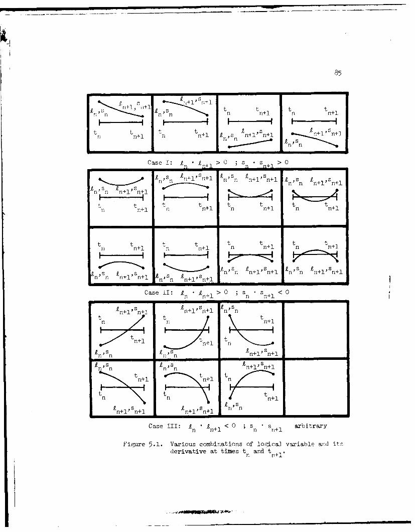
85
£ ~ n+1, 11+ ' t t t tn+
t t t t A sYHn+1 n nA-1 I ns n 4l l t : n+1,n + 1
Case 1: e ~0 ; s, , >0
n n+ n n+
In ~~+1 Sn+ n £~'
t 1tnl tn + t l tntn1tl n A-i
n
t1 t n+i t n+ t n n1 tntn
Is s Istn1 +1 1 " 'sn l~
Case II: I >n1 0 ; s - ris < ritar
Figure~ 5.1 Vaious conatons o l~a aial ndeiatv at times t ant
n+ nnA-n

86
methods are employed in many predictor-corrector integration algor-
ithms: 1) a Nordsieck vector representation, which stores k deriva-
tives of the state variables at time station tn [ 44 ], and 2) ath
divided difference table, based on the t and previous k values ofn
the state variables [ 45]. Root finding techniques for each method
are straight forward and will not be elaborated upon here.
5.3 Intermittant Motion in Constrained Systems
The phrases "discontinuous forces", "impulsive loads", and
"discontinuous motion" appear often in the literature. In a micro-
mechanics sense, such phenomena do not exist. However, to an
observer who is interested in the dynamic response of systems over
long periods of time, the idea of "discontinuous" or "impulsive"
may be quite satisfactory. On the other hand, an observer interested
in system dynamic response over short periods of time, specifically
during significant events, will treat them in a continuous manner.
Discontinuous and impulsive are thus labels that may be placed on
continuous events, which in a macro-mechanics sense are effectively
represented as discontinuous or impulsive in the observer's time
frame. This illustrates the desirability of pieced interval analysis
for certain applications, where entirely different mathematical
models (and possibly analysis techniques) may be employed during
different intervals of system motion.
In this section momentum balance equations are developed from
Lagrange's equations of motion, assuming that discontinuous external
forces or impulses are applied to a constrained system. The equations

87
are initially written for the case in which these events occur in a
finite amount of time. It is assumed that the time interval -, 'r2)
is small enough that the system configuration does not change
appreciably, that is, q(T2) (q(T). In addition, the constraints
in Equation 3.1 are continuous fur, ,ions of q and t.
I I IT1 ti T2
Figure 5.2. Event interval
Let t° be a point in time at which a "violent event" occurs,
which is to be approximated by a discontinuity. In reality, the
event occurs over a time interval T < t i < T2Y as shown in Figure
5.2, and behavior is smooth except possibly at t. Integrate
Equation 4.8 to obtain
T 2 [m w + H T Mu v + (M vu + HT M UU)HIV dt

88
f [A + Q' + HT(AU + Qu)
-(M v u + HTMUU)'*]dt (5.3)
Since H is differentiable, integration by parts and using the
mean value theorem gives
T 2
[Mw + HTMuv + (Mvu + HTMuu)H] IT
v2 d [Mvv + HTev + (kvu + HTMuu)Hj-
+ Av + H TAu _ (Mvu + HTMuu)'U*]dt
r Qv dt + TfQu dt (5.4)
T1 1
Where H is a matrix whose elements are those of H evaluated at points
in (TI 1'2).
Treating Q as impulsive at t, the integrals of generalized
force are "generalized impulse",
p Qvdt and Pu = 2 Q Udt
T

89
Taking the limit in Equation 5.4 as T 4 ti and -2 4 ti' noting from
Equations 3.19 and 3.22 that U is bounded so A + H A - (Mvu
+ HTMUU )U* is bounded, yields the "impulse momentum" equation at t.1
as
M + HTMu v + (Mvu + HT M UU)HI [(ti+) - -(ti-)]
=pV + H TP u (5.5)
This prescribes the velocity jump in v due to impulsively applied
loads.
It is important to note that Equation 5.5 involves impulse
and momentum of all elements of the mechanical system. This is
crucial, since the bodies making up the system interact through con-
straints, so an impulse-momentum balance relation involving only the
bodies on which the impulsive force acts is impossible. Deriving the
relation of Equation 5.5 by manual calculation would be extremely
difficult and time consuming. One of the strongest points of the
method presented here is the automatic assembly of the coefficient
matrices of Equation 5.5.
i
(+f(t)
j
Figure 5.3. Impacting bodies

90
For impact of bodies i and J, as shown in Figure 5.3, acoefficient of restitution e provides the relative velocity relation
in direction i7 (where !T is taken as a row vector) as
[ (ti +) qJ(ti+)J = " e- [4 (t-) - (t.)] (5.6)Ti 3n i
or with NTE R~ , u N , NV . Equation 5.6 may be written
Nv v(ti+) + NU i(ti+) =- e Nv + Nu .1 N (ti-) N u(ti~)
or using Equation 3.17, this is
[NV + NU H (ti+) + Nu *
= - e [NV + Nu (ti-)-e Nu u*(t -)(57)
Equation 3.16 implies that u* is a function only of q and t and con-straints are continuously differentiable in q and t. Therefore,
(ti+ ) A(ti- ) and Equation 5.7 reduces to
[Nv + NU H] 4(t.+) = - e [Nv + Nu H] i(ti-)
(e + ()Nu (t)8)

91
The generalized impulse of the force f(t) in Figure 5.3 is
t i+P f(t)NTdt = pNT (5.9)
where
t.+E
p J ff(t)dt (5.10)t.-C
T TDefiingthe partitioning P"pV N p
Defining pNv and P pN , Equation 5.3 gives
[M' + HTMuv + (vu + HTMuu)H][,(ti + ) -(t -)A
T T=p [Nv + HTN ] (5.11)
The above equations are put into matrix form for solution as
follows. Subtract the identity
[Nv + NUH] (ti-) = [NV + NuH] -(ti-)
from Equation 5.8 and define
A-i = - (ti+) - (ti-) (5 12)

92
The matrix equation thus becomes
[jv + HM + (vu +HTMuu)H (NV + H * [:: I(N Nu H)0
~0
+ l) (Nv + Nu H)(ti-) + Nu i* (t1-) 1 (5.13)
whose solution yields the desired velocity jumps and magnitude of
impulse at the body surfaces.
5.4 Pieced Interval Computational Algorithm
The development in this and previous chapters is combined into
a general pieced interval analysis algorithm. In the discussion to
follow, for notational convenience, assume that logical variable
J identifies ti, the end of the ith stage. Associated with ji is a
set of system state equations for the (i + 1)st stage (which may be
dynamic equations of motion or momentum balance equations). In
addition, a different set of constraint equations 0i+l (which may
include boundary constraints .n velocity) may be used at this stage.
i+lA different set of logical functions 0? , compatible with the above
constraint and state equations, may also be introduced.

93
Prior to implementing the algorithm, it is assumed that all
possible system events have been anticipated and appropriate logical
event predictors and corresponding constraint and state equations
have been formulated. Knowledge of the sequence of events is unneces-
sary, unless this knowledge can be used to reduce the complexity of
equation formulation. Further, it is assumed that no event takes
place prior to achieving the initial static equilibrium configuration
or appropriate initial conditions at time t = to.
The computational algorithm is as follows:
Step 1. Obtain initial conditions consistent with constraints,
using the algorithm of Section 4.3.
Step 2. Select the appropriate set of state equations, con-
straints, logical functions, etc., based on the current active logical
events monitor flag or continue with previous equations.
Step 5. If a momentum balance is required, solve for velocity
jumps as in Section 5.3 and return to Step 2.
Step 4. Using the techniques described in Section 5.2 check
for active logical variables (one or more 2J passing through zero) in
the next time step to be attempted by the numerical integration
algorithm. Solve for time steps corresponding to the zeros of poly-
nomial predictors of active tJ (if any), set the integration time
step to the smallest step (first occurring 1J) and set the corres-
ponding logical events monitor flag. Advance the solution to this
point in time by executing Step 5.

94
Step 5. Perform dynamic analysis using the algorithm described
in Section 4.4. If the solution is advanced by the above time step
return to Step 2, unless the end of the simulation interval is
reached, in which case stop. If a smaller time step is taken to
meet integration error requirements, reset the logical events moni-
tor flag (since the event has not yet been reached) and return to
Step 2.
5.5 Sparse Matrix Considerations
To maintain program efficiency when mechanical systems become
large, sparse matrix algorithms should be employed and matrix
products avoided. The methods of sparse matrix computations described
in previous chapters will replace the corresponding full matrix
operations in the algorithm of Section 5.4. It is possible to show
that Equation 5.13 can be expressed in a form suitable for sparse
matrix computations by first writing it in permuted form as
Mum Muv nT NT AiM uu M uV vu Tv
vu M T NV
Ou 0V 0 0 -Nu Nv
N NV 0 - p

A
95
0
0
n
[ ],U NV
e ' (ti-) + N' (ti-)3 (5.14)1 L
where . is a vector of Lagrange multipliers. This equation is
equivale'i to the unpermuted matrix equation
T NT .M I q Aq
0 0q
N 0 0 -p
0
= 0
-fe + 1)[N 4(ti-)) (5.15)
To show the equivalence between Equation 5.13 and 5.14 carry out
the matrix products in Equation 5.14
TAi + M - Nu p= 0 (5.16)
..- -------

96
Mv u Av + i - v x - Nv Tp = 0 (5.17)
=u Ai + 0v i = 0 (5.18)
Nu A + NV (e + 1[Nu u(ti') + Nv v(ti-)1 (5.19)
Since
Ou Aui(t i " + § v i(t i-) + @t(t i" = 0 P
Ou A, (ti+) + 0v i(ti+) + t (ti+) = 0 P
and
§ t(ti-) = t(t i+ )
then
uUI(ti+) - ui(ti-)) + Iv1ti(ti+) - 'i(ti-)] : 0
and Equation 5.18 is satisfied. Equation 5.18 also implies that
Ai = -u1 Ai =H A i (5.20)
i v

T
Equation 5.19 is simply the second equation of Equation 5.13
where Equations 3.17 and 5.20 are employed.
Since u T is nonsingular in Equation 5.16, solve for Z and
substitute into Equation 5.17, thus
Mvu . Mw A~ i + T u-T . u i _ v .+ v i
T T+ Nu p) - Nv p 0
Combining terms and using Equation 5.20 yields
T HT
fM + HTMu v + (Mv u + HTM )HA V- (Nv +H )p = 0
which is the first equation of Equation 5.13. Equation 5.15 is thus
solved to determine changes in velocity due to impact between bodies.

98
CHAPTER 6
NUMERICAL EXAMPLES
6.1 Introduction
Numerical examples are presented to demonstrate generality
and improved program efficiency, resulting from the analytical methods
developed in previous chapters. Generality is demonstrated by the
ease of representing models of complex dynamic mechanical systems.
Efficiency is demonstrated by contrasting computer simulation times
for the various solution methods.
The analytical methods developed In Chapters 3 and 4 demon-
strate the greatest improvement in program efficiency when mechanical
systems are heavily constrained. The integration algorithm of
Chapter 2 iteratively solves (6n + r) differential and algebraic
equations, whereas the algorithm of Chapter 4 solves 6n - 2r dif-
ferential equations; n being the number of system rigid bodies and
r the number of independent algebraic constraint equations. Defining
system degree of freedom as
dof = 3n - r
the ratio of number of equations for the two methods is

99
(6n - 2r)/(6n + r) = (2 dof)/(9n - dof)
For systems with many bodies and a few degrees of freedom, this ratio
is small.
The three degree-of-freedom link gear multiplier consisting
of twelve bodies, shown in Figure 6.1, has an equation ratio of
0.057. The one degree-of-freedom Peaucellier Lipkin mechanism in
Figure 6.2 consists of 8 bodies and has an equation ratio of 0.028.
A significant reduction in matrix and numerical integration opera-
tions is expected. Increased efficiency also results from the use
of single precision computer arithmetic, reduced number of corrector
iterations, and larger time step sizes.
Operations count for solution of sparse matrix problems is
of the order N. where N is the matrix dimension [46 1. The ratio
[(3n)/(9n - dof)]1.6 is a rough estimate of the reduction in opera-
tions count. When dof << 3n this ratio approaches 3( 1.6) = 0.17.
As dof -+ 3n the modified constraint matrix (see Equation 3.36)
corresponding to the numerator of this ratio approaches an identity
matrix, requiring substantially less than (3n)1 .6 operations. More
than a 10 to 1 reduction in simulation time for the above mechanical
system simulations was observed.
As the equation ratio increases, one expects less gain in
program efficiency. For example, the mechanical system described
in the next section, consisting of 12 bodies with 24 degrees of
freedom, has an equation ratio of .596 and a corresponding 4 to 1
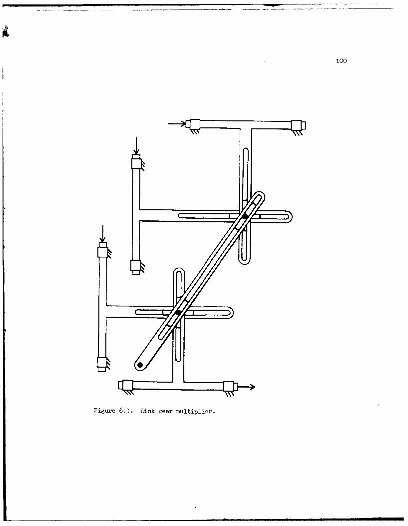
100
Figure 6.1. Link gear multiplier.

Figure 6.2. Peaucellier Lipin mechanism.

102
reduction in execution time. Note that the above equation ratio for
both methods includes 5 additional differential equations that
describe control system dynamics. Another mechanical system (not
presented in this report) consisting of 8 bodies and 13 degrees
of freedom, has an equation ratio of .44 and a corresponding 7 to 1
reduction in execution time [21]. Matrix operation counts also
play important roles in reduction of computer time.
6.2 Two Articulated Army M-113Armored Personnel Carriers
(a) Vehicle Pitch Position and
orce Feedback Control
A research test vehicle shown in Figure 6.3 was built by the
Army for the purpose of investigating off-road performance of
articulated tracked vehicles [47, 48]. This vehicle is selected
for simulation here, because most of its parameters are known, some
field test data is available for comparison purposes, and its pitch
articulation (while negotiating terrain and obstacles) can be
adequately represented by a planar model.
The test vehicle consists of two identical M-113 Army armored
personnel carriers, coupled together by a spherical ball socket that
allows relative vehicle pitch, yaw, and roll. This connection is
located close to the rear of the front vehicle, to give the rear
vehicle an increased moment arm, thus allowing it to remain nearly
horizontal as the front vehicle is elevated. This allows the
articulated vehicle to negotiate step obstacles up to 5 feet in height.

1 03
. . .. . . . . .. .

Relative pitch and yaw motion; of the ::ystem is controll,i by
two hydraulic cylinders acting between the veiclo.m a!- :;ho!
Figure 6.3. Yaw motion occurc when one cylinder ex ten&. an, th,
other simultaneously contracts. Yaw will not be considercd ii this
investigation. Therefore, equal actuator lengths, thu. -quQ u-
ator exter~ion and contraction rates, will be assumed. The hy.rauli,
control system is capable of maintaining equal actuator extensin
rates, while negotiatinq various obstacles.
Relative pitch and yaw can be controlled by the vehicle
operator, via a control stick. If the stick is pushed to the right
or left, the front vehicle yaws to the right or left, respectively.
If the stick is pulled back or pushed forward, the front vehicle
pitches up or down, respectively. Combinations of stick movemnents
yield general yaw and pitch motions. It is assumed that only pitch
command signals are given in the following planar simulations.
For the operator to relate control stick displacement to
relative vehicular pitch displacement, a proportional control is
required. That is, pulling the stick halfway back causes the vehicle
to pitch up to 50 of its maximum allowed displacement, etc. Pro-
portional control is provided through positional feedback to the
control system by monitoring the hydraulic actuator extension or
contraction. Proportional yaw control is obtained by a similar
process.
Typical operator actions for negotiating a terrain obstacle
might be as follows: To negotiate an obstacle pull the stick back

105
fax enough such that the front unit can mount the obstacle. Gradu-
ally drive forward while adjusting stick position so that the vehicle
maintains maximum conformity to the terrain and obstacle. This
technique generally gives the smoothest ride and better vehicle
traction and control. However, the operator must uontinually observe
the vehicle's position relative to terrain, in order to make these
adjustments. This requirement may limit his ability to perform other
tasks.
Maximum terrain conformity is achieved if the hydraulic
actuators are removed from the vehicles. Since this isn't possible,
the alternative is to maintain zero pressure within the actuators.
This is accomplished by providing force feedback from the hydraulic
actuators to the operator, via the control stick.
Suppose the operator pulls back on the control stick and the
vehicle begins to pitch up. Pressure builds up in the rod end of
the cylinder and a voltage from a pressure transducer is generated.
This signal is amplified and applied to an electro-mechanical device
that pulls forward on the control stick, thus increasing its resist-
ance to the operator's applied force. This gives him a feel for the
pressure within the hydraulic actuator. He has simply to move the
control stick in the direction it wants to go. In fact, he may
remove his hand and the control stick will automatically position
itself for minimum pressure and best terrain conformity. Therefore,
force feedback allows the operator to devote more of his attention
to other duties.

lO6
The control system cannot respond to system pressure changes
instantaneously, because of inertia and hydraulic system compliance.
Thus, at best, it can only maintain a zero average pressure over some
time interval when the vehicles experience rapid relative pitch
displacements. In fact, pressure transients may become quite high,
as evidenced in results of simulations. A complete description of
the electro-mechanical-hydraulic control system model is given,
following a description of the vehicular system model.
(b) Elements of the Articulated
Vehicle Mechanical Model
The primary components of an M113 APC are the chassis and ten
roadwheels, five per side. The roadwheels are connected to the
chassis by roadarms that are rigidly attached to torsion bars that
provide chassis suspension. Each vehicle has two front drive and
two rear idler sprockets. Segmented tracks, as shown in Figure 6.3,
pass beneath the roadwheels and around the sprockets to form contin-
uous loops. Power is transferred from the engine to drive sprocket
and then to track that propels the vehicle. The roadwheels simply
roll along the inner track surfaces. Shock absorbers provide damping
in the front and rear suspensions.
A representative planar model is established from the above
description. It is cost prohibitive to establish a model that
minutely simulates the actual system. Therefore, various simpli-
fications can be made where minor effects are ignored. Since motio!1
in a plane is considered, model symmetry is employed to reduce

107
problem size. It is supposed that opposing roadwheels experience
equal displacements, hence can be combined into single bodies having
double mass and rotational inertia. Suspension stiffness and damping,
track properties, etc., are doubled.
Track dynamics is not being studied here, so the mass and
rotational inertia of the track segments beneath roadwheels is equally
distributed among them. That part of the track supported by the
chassis is lumped with the chassis mass and moment of inertia. Track
supportive effects on chassis and roadwheels are significant and will
be included in the model.
An outline drawing of the nodel is shown in Figure 6.4. This
model consists of 12 bodies, two chassis (B11 and B12) and ten road-
wheel pairs (BI to B1O). Roadarms, represented by massless links
described in Chapter 2, connect roadwheels to the chassis. To
simplify a track model, roadw'heels are free to rotate, but only small
rotations about initial angular positions are considered. Large
rotational displacement of roadwheels is prevented by the track model.
Vertical force versus vertical roadwheel-displacement-suspen-
sion curves and vertical force versus vertical roadwheel-velocity-
damping curves were determined experimentally (Figures 6.5 and 6.6).
These forces are incorporated into the model employing features of
the standard spring-damper-actuator elements described in Chapter 2.
Elements S1 to S10, connected between chassis and roadwheel centers,
are given arbitrarily long lengths; i.e., 1000 inches so that their
forces relative to chassis remain essentially vertical for all

108
N N- N
a) U
0Uf) W
0))0
-
qH
0
00)
U)U
to nit) 03
UU)
N (
(n N

lo9
-5000 04 01 roadwheel # 1
20000-
ci 0 roadwheel 2, 3,
S 15000 -
" roadwheel # 510000 -
o 0C,
0- 2 4 1
displacement (inches) 4 jounce
Figure 6.5. Torsion bar suspension characteristics
4ooo -
3000 -
e 2000.
0
1000
1,- 44 0
C) -10000
i2000I
- 100 - 75 -50 -25 0 25 50 75 100
velocity (inches/second) 4 jounce
Figure 6.6. Suspension damping characteristics

110
roadwheel positions. Vertical roadwheel displacement relative to
chassis is given by (Ioij Iij ), where 9,j is the current element
length and tc0 is a constant reference element length. Verticalij
roadwheel velocity, relative to the chassis, is given by (- ij).
These standard variables are available to user supplied subroutines
in the program. Taking k i and cij as zero in Equation 2.9 yields
an actuator element force of
ij = F O i j (%slj /I j)
Suspension and damping force functions Fs (oi j - ij) and Fd(- iij )
are supplied by cubic spline curve fits [49, 501 to the data
(straight line approximations have been successfully employed as
well) [ 51]. The actuator force, evaluated as
Fo = Fs(Oj - LI .) + Fd( " Ai )0i ij oij ij 1i
is automatically added to the system generalized forces.
(c) Elements of the Track and
Terrain Interaction Model
Track forces on the chassis and roadwheels are included
through spring-daper elements S11 to S22 (Figure 6.4). It is assumed
that roadwheels remain in contact with the track throughout the simu-
lation. Therefore, elements are connected directly to the bottom of
the roadwheels. Elements Sll, S16, S17, and S22 are also connected

directly to the chassis at the approximate points of track tangency
to the drive and idler sprockets. These elements provide track
interaction forces between the chassis and roadwheels. Each element
segment has an effective stiffness determined by its approximate
length and a track stiffness per unit length. Internal track damping
is included to account for rubber bushing, rubber track pad, and
ground dissipation. These coefficients depend nonlinearly on track
displacement, since track segments cannot support compression.
Tracks are given a pretension so they will remain tight in
various dynamic situations. Each element SI1 to S22 is thus given
an initial pretension of 10000 pounds. In order to determine changes
in track tension (from equilibrium preload levels), due to dynamic
loading, it is necessary to have reference track lengths 10i j = Iij
at equilibrium for each of the above elements. These lengths cannot
be determined when the model is established, because the equilibrium
configuration is unknown. They can be evaluated directly by the
program as equilibrium is established as follows: Set k.. = c.. = 0
and F0 = 10000 lbf in Equation 2.9 for each element S11 to S22.
Constrain angular rotation of each roadwheel, using initial condition
flags on input data cards to keep element attachment points at the
bottom of the wheels. Solve for equilibrium and set each element
e0 to it., which then becomes the reference length for dynamic
analysis. Equation 2.9 for the lynamic track model then becomes
Fij = [kij(Aij)(Iij - t0 + cij(Iij)iij + F0 ] [ S
ii i~j

112
where k.i( ti) and c. (YC.) are determined to prevent the coefficient
of [i /.e i from becoming negative.
Roadwheels must be prevented from penetrating the terrain
surface. That is, penetration should be no greater than that achieved
by local wheel, track, and ground deformation. Support generally
occurs at one or more points on the lower arc of a wheel, due to
direct terrain contact or indirect track support. Support reaction
forces may not act vertically. The general model for arbitrary
terrain is rather complex. For the current discussion, assume a
level terrain (a more representative model for irregular terrain is
presented later), hence roadwheel support reaction forces remain
vertical. These forces may then be moved to the wheel centers with-
out changing the model. Since roadwheels are circular, the terrain
reference elevation can be shifted up to the wheel centers for deter-
mination of relative wheel-terrain elevation. Global location of the•thi roadwheel center is given by coordinates xi and y (see Chapter 2).
If gi is global terrain elevation and rw is roadwheel radius, then
wheel penetration into level terrain is
Pi = (gi + rw - Yi)
If wheel reaction force is developed according to the curve in
Figure 6.7, the force Fw(Pi) is then added to Qvi (see Equation 2.10).
If pi 0, F w(P ) = 0 and the i t h wheel is not touching the terrain.
A damping force DW(Pi, G, with hi= - is also added to

III
113
10000 -
35000
30000
25000
20000
1500
0CHS 15000
10000
5000
0
0 .5 1.0 1.5 2.0 2.5 3.0
penetration (inches)
Figure 6.7. Roadwheel-ground force--penetration curve.

1114
iQy to include roadwheel rubber-, track rubber-, and ground-damping
effects. Damping force Dw reduces to zero as pi decreases to zero.
When vehicle pitch displacements are large, other points on
the chassis may contact ground. The most likely places are the drive
and idler sprockets, labeled A to D in Figure 6.4. Sprocket centers
are located by global points x and y . With sprocket radii rP pi cione may obtain support and damping forces as above. These forces
are then included in generalized forces Q and Q ,'for the proper
bodies.
As noted in earlier discussion, the usual procedure for
representing wheel-terrain interference is to monitor the distance
between the bottom point on the wheel and the point on the terrain
directly below it. If, as in Figure 6.8, the terrain slopes or is
irregular, other points on the wheel may make first contact. Thus,
the wheel will be at an incorrect height and the support force on the
wjel will act incorrectly. A modified wheel trajectory may be
.bbtained by moving a rigid wheel of a given radius, say that of the
roadwheel, along the terrain surface to obtain a trajectory of the
lowest point on the wheel [52 3. The wheel trajectory for the terrain
in Ft gure 6.8 is shown in Figure 6.9. As the lowest point on a
wheel follows this trajectory, th're will always be some point on the
wheel just touching the terrain, but there will be no terrain penetra-
tion. This is illustrated in Figure 6.10. For the purpose of this
simulation, it is sufficient to assume that the resultant support
force vector acts along a line passing through the point of

115
y
Figure 6.8. Terrain contour of 36 inch step obstacle.
a' -'m i ln lmI.~. h .. , .. ....o

116
I
FIgure 6.9. TraJectory of 12 inch wheel rolled over a 36 inch stepobstacle.

117
x
Piure ,.i0. Wheel trajectory defined by lowest points on wheel withno terrain penetration.

118
wheel-terrain contact and wheel center. Thus, there will be a com-
ponent of force tending to impede leftward motion of the wheel and,
if not otherwise supported, the wheel will move down the slope. The
angle that this force makes with respect to the positive y axis is
shown in Figure 6.11. The curves of Figures 6.9 and 6.11 are pro-
vided to the program in the form of cubic spline functions.
The normal and frictional components of force acting on the
wheel remain to be determined. As noted earlier, if global
coordinates xi and Y locate the center of a roadwheel and if g(x.)
is the trajectory height beneath the wheel, as in Figure 6.9, then
wheel penetration may be approximated by
Pi = [g(xi) + rw - Yi] (6.1)
where r is the roadwheel radius. Normal force angle, from the
function h(x) of Figure 6.11, is
(I = h(xi) (6.2)
Figure 6.7 illustrates a typical nonlinear force-displacement rela-
tion between a roadwheel and ground. Let this curve be represented
by the function f(xi), so the total vertical force acting on the
wheel, as shown in Figure 6.12, becomes
FS = Fny + Ffy = f(p) (6.3)

119
0 radians
x _ -14 radians
Figure 6.11. Direction of a line passing through point of wheel-terrain contact and wheel center.
':! 1

120
where Fny and Fly are the vertical components of the normal, Fn a 0,
and frictional Ff forces, respectively. The subscript i has been
dropped for convenience. In terms of the angle Ce and the sign con-
ventions of Figure 6.12, the following expressions hold:
F = - F sin anx n (6.4)
F = F cos tny n
F fx = Ff cos 0 sgn (slip)fx f(6.5)
Ffy = Ff sin c sgn (slip)
fy fX
F
nx
Figure 6.12. Terrain-wheel contact forces.

121
where positive slip occurs if the wheel slides to the right. The
wheel may not slide, in which ease there is some force F' such thatf
JF4j < IFf1 (6.6)
If the coefficient of sliding friction is p, then the resulting
frictional force is
F f mn (IF.t or 4Fn) s (slip) (6.7)
Equations 6.3 to 6.7 can be combined to derive an expression for the
frictional force, in terms of the vertical force FsP
Ff = min [1Ffl or (pF )/fcos a - . sin ce sgn (slip)}]
x sgn (slip) (6.8)
The vehicles propel themselves along the terrain, so driving
forces are applied to the track and roadwheels to achieve this goal.
For simplicity, it is assumed that the vehicle is to travel at a
constant velocity across the terrain. Denote this velocity as vr
and the desired lateral displacement as S rj = SOj + vr t, j = 11,12,
where SOj is the global location of a reference point on the j th
vehicle at time, t = 0. Locating this point at ground level and at
the center of the vehicle will secure an approximately constant

12;
ground speed. Let v. be the actual velocity of this point on body j
at any instant t, then the actual displacement of this point is
tSj sOD + 1 v.dt (6.9)
0
Track tension is developed according to error in the desired
vehicle position and velocity as
T = K d(S - S rj) + Kv (vj - v r) (6.10)
where the constants Kd and K are chosen to characterize the vehicled r
power train. Observe that T. may be positive (vehicle lags behind
desired position) or negativ (vehicle is ahead of desired position).
If T. > 0, T. is applied to track elements S16 and S22. If T. < 0,
- T. is applied to track elements Sll and S17. The maximum tractive
effort is limited to the maximum force developed by a slipping track.
The sequence of steps to evaluate track driving forces for the
front vehicle are described. If T > 0, set F' = T . Find F for
sprocket C, as shown in Figure 6.4, using Equation 6.3. Assume slip
> 0 (Figure 6.12), since the vehicle is being propelled to the left.
If Fs = 0, the sprocket is not in contact with the terrain. Therefore,
no frictional tractive force is developed beneath the sprocket, so
the entire force F' is transferred to track element S16.
If sprocket C is in contact with ground, F > 0. Therefore,s
determine the frictional tractive force Ff acting between sprocket
fm, mnm = = mmn mmm u dm m nm l ll ml nm l l
123
and ground, using Equation 6.8. Apply Ff to the sprocket at the
point of sprocket-terrain contact, directed along the tangent to the
terrain surface at this point. The track driving force F" is now
reduced by Ff and is applied to track element S16. The procer is
then repeated in a similar manner for each successive roadwheel,
rear to front. Calculate F for roadwheel (B5) from Equation 6.3 and
Ff from Equation 6.8. Apply Ff to roadwheel (B5) at the point of
roadwheel-terrain contact, directed along the tangent to the terrain
surface. Again reduce F' by Ff, and apply this force to element S15.
Continue this process until F' has been reduced to zero, or until
sprocket D has been passed. If F' becomes zero, the vehicle is not
traction limited. If F' > 0, the track is slipping and the desired
reference position, S r in Equation 6.10, cannot be attained; so set
S = S. - v rt and S = Si, the attained vehicle displacement.
If T. < 0 in Equation 6.10, the process is reversed. That is,
drive forces are applied from front to rear. First check sprocket
!, roadwheel (Bl), etc. for contact and apply appropriate forces.
The vehicle is bei. g driven to the right in this case and slip is
assumed to the left (Figure 6.12), hence it is negative.
The significant feature of this model is that track slippage
at each wheel is allowed if there is enough force differential in
the track to overcome local friction pF.. The remaining road wheels,
once F' becomes zero, are assumed to have zero frictional forces
acting. This will not be true for the actual system, especially on
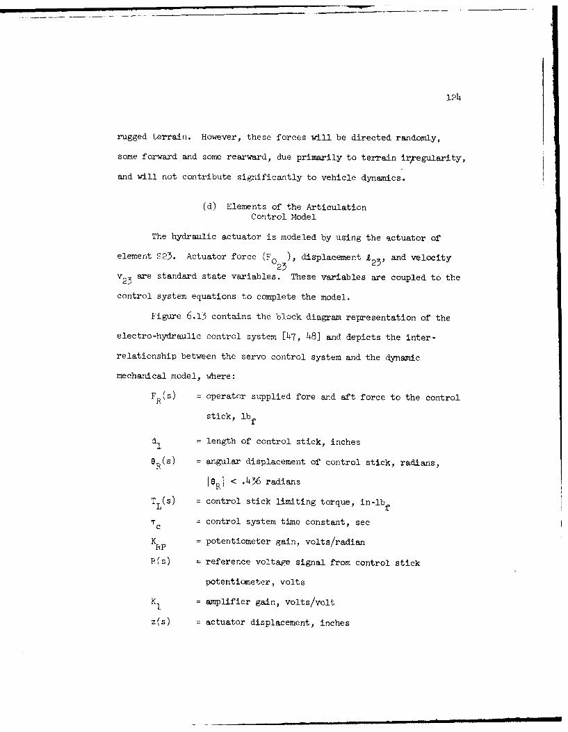
124
rugged terrain. However, these forces will be directed randomly,
some forward and some rearward, due primarily to terrain irregularity,
and will not contribute significantly to vehicle dynamics.
(d) Elements of the ArticulationControl Model
The hydraulic actuator is modeled by using the actuator of
element S23. Actuator force (F0 23), displacement 123' and velocity
v2 3 are standard state variables. These variables are coupled to the
control system equations to complete the model.
Figure 6.13 contains the block diagram representation of the
electro-hydraulic control system [47, 48] and depicts the inter-
relationship between the servo control system and the dynamic
mechanical model, where:
F R(S) = operator supplied fore and aft force to the control
stick, lbf
d = length of control stick, inches
eR(s) = angular displacement of control stick, radians,
leRI < .436 radians
T L(S) = control stick limiting torque, in-lbf
T e = control system time constant, sec
K RP = potentiometer gain, volts/radian
P(s) = reference voltage signal from control stick
potentiometer, volts
K = amplifier gain, volts/volt
z(s) = actuator displacement, inches
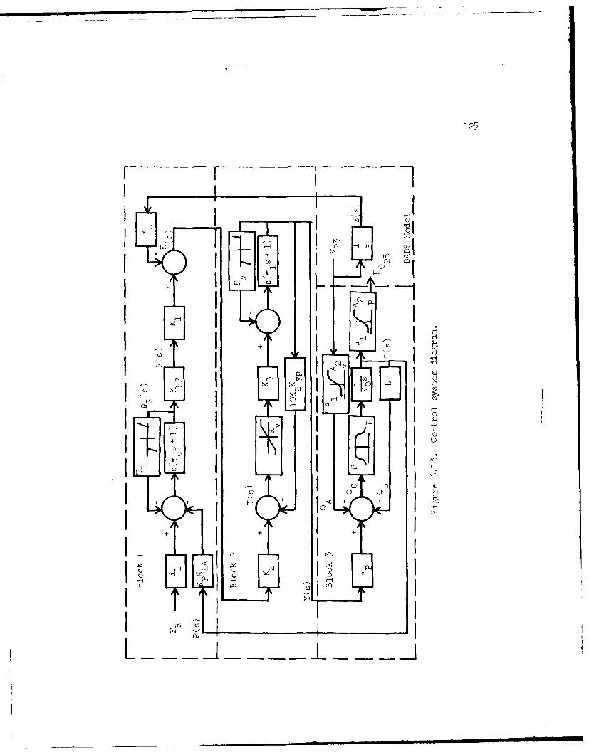
125
cHa
I N,
~Cd
I 0H
I I Kn
I 11110

126
1 23(s) = total actuator length, inches
t 0 23 = reference actuator length, inches
v 23(s) = actuator velocity, in/sec
K 4 = actuator potentiometer feedback gain, volts/in
E(s) = error signal voltage, volts
K2 = amplifier gain ma/volt
I(s) = amplifier current, ma
K = servo valve flow gradient, GPM/mav
K3 = pump stroke mechanism velocity gradient,
% stroke/see
T1 = servo valve time constant, sec
Y(s) = pump yoke displacement, 1, stroke
Fy(s) = pump yoke limiting force, lbf/in
Q% = pump flow gradient, (in 3/sec)/(% stroke)
Ir = pump flow, in 3/sec
QA = load flow, in 3/sec
QL = leakage fiow, in 3/sec
Q= flow due to compressibility, in 3/sec
A1 = actuator area - rod end, in 2
A2 = actuator area - cylinder end, in2
e = effective bulk modulus including system compliance,
psi
VO = entrained volume of hydraulic fluid
L = combined system leakage coefficient, (in3 /sec)/psi
P(s) = system pressure at the actuator, psi

127
p0 = force developed in the actuator, lbf
K = pressure transducer gain, mv/psip
= control stick force feedback gain, in-lbf/mv.
The articulated vehicle control system may be divided into
three major blocks. As shown in Figure 6.13, block 1 generates a
reference voltage that ultimately leads to a given hydraulic actuator
displacement. The major component in this block is the mechanical
hardware that interfaces with the operator. Block two contains the
hydraulic pump yoke and servo valve control system. In response to
an error signal from block 1, this system controls direction and
fluid flowrate in the hydraulic pump. Block 3 characterizes dynamic
response of the hydraulic system, including the actuator connected
to the articulated vehicle model.
The control stick, showii iii Figure 6.14 P17 ], rotates about
a fixed point. A direct current linear actuator, shown in its neutral
position, is coupled to an extension of the control stick d2 by
springs K1 and K . These springs provide restoring moments to main-
tain the control stick in its neutral position. In response to
pressure buildup in the hydraulic actuator, a voltage is developed
across the linear actuator, causing springs K1 and K2 to shift either
left or right. An increased moment is then developed on the control
stick to oppose the operator supplied force, thus providing force
feedback to the operator. In addition, mechanical stops prevent
more than t 250 rotation of the control stick. The dynamics of this
system, including inertial effects, is included in block 1. Control

128
stick response is determined by three moments: operator's moment,
(FR * dI ); pressure feedback moment, (-Kp KLA P); and mechanical
stop limiting torque, [- T L(e)].
A rotary potentiometer connected to the control stick develops
a reference voltage that is proportional to angular rotation R .
This signal is then amplified and combined with a hydraulic actuator
displacement signal (- K 4 z) to obtain an error signal E. This
error signal is then amplified and passed to the pump yoke control
system.
Servo valve and pump yoke characteristics are illustrated in
block 2 of Figure 6.13. Significant nonlinear effects in the system
B (t)
forward
dI1
rotary potentiometer
K 1 d2 c onnecting cable
" sprigs 2- D.C. linear
. . .. I actuator
+ x(t) >- X(t)
Figure 6.14. Contro] stick and force actuator.

129
are saturation of the servo valve flow control K and mechanicalV
limitations on pump yoke displacement F . Inertial effects in thisy
block introduce additional delay in overall system response.
Block three outlines the hydraulic flow model. Flow rates
within the system are moderate, so pressure drop within the lines
is small. This simplifies the model significantly. The pump
supplies fluid volume flow rate Qp, to make up for leakage losses
QL' compressibility QC' and actuator volume displacement rate ,A'
The system contains a significant amount of flexible tubing,
which results in reduced system compliance, hence a small effective
bulk modulus. Pressure limiting is obtained by further reduction of
the effective bulk modulus, as relief valve blowoff begins. Actuator
flow rate from the pump is determined by the product of actuator
cross-sectional area A and velocity v. The area A on the rod end
of the actuator is smaller than the piston end area A . Thus, area
is adjusted appropriately as a function of actuator velocity to
achieve the proper flow rate. Force developed in the actuator also
depends on which side of the piston pressure is developed. Thus,
area is adjusted as a function of pressure, for the purpose of
calculating actuator force. The controller consists of two identical
hydraulic systems, each driving an actuator. In this simulation,
only one hydraulic system is modeled, so the effective actuator
force is doubled to account for two actuators.

130
(e) Crossing a Three-Foot ObstacleNumerical Results
The three-foot step obstacle shown in Figure 6.8 is selected
to test the program's ability to adequately describe system dynamics.
In addition, the effect of force and position feedback on vehicle
performance, while negotiating a significant obstacle, is to be
investigated. A velocity of 40 inches/second (2.27 miles/hour) is
selected as the obstacle crossing speed. This is close to the
design specifications of minimum 2.5 miles/hour over a 2.5 foot
obstacle.
Contrary to usual practice, the vehicle is not put into an
initial pitch up attitude before encountering the bank, but is forced
to propel itself up the side of the bank. The vehicle is run in a
hands off mode, because it is difficult to program operator response
to the complex dynamic environment.
Three simulations of obstacle crossing are performed. The
first case is with force and position feedback active, the second is
with force feedback deactivated, and the third is with the entire
control system deactivated. In the last situation the control system
is passive, except that the hydraulic pump is providing enough fluid
flow rate to replace leakage losses. A sequence of computer generated
line drawings of vehicle position at one-second intervals for the
three cases is shown in Figures 6.15-6.17.
The following observations can be made from these figures.
Force and position feedback in Figure 6.15 tend to minimize actuator

t=0 t=c
t t 9
f 4 t =10
t=5
Fifpure 6.15. Obstacle crossing with force and position feedbackactive - ten second simulation at 40 inches/second.

132
t =0 t =6
t 1 t =7
t 2 t =8
t 3 t =9
t 4 t =10
t 5
Figure 6.16. Obstacle crossi'Og with force feedback deactivated -ten second simulation at 40 inches/second.
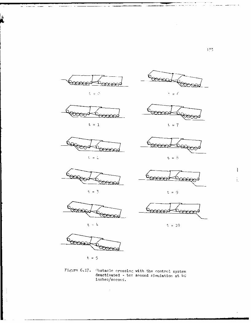
+177
t 1 t 7
t = t=
t - t =10
t=5
Fivure 6.17. Obstacle crossing with the control systemdeactivated - ten second simulation at 40inches/second.

134
stiffening of the coupled vehicle system. This will be the most
comfortable and stable situation since the vehicles tend to conform
to the terrain.
Position feedback alone in Figure 6.16 tends to maximize
vehicle rigidity in the hands off mode because the control system
continually works to maintain minimum departure from the zero
relative pitch position. With operator assistance, however, one
might exoect vehicle response approaching that of case 1.
The -assi model in Figure 6.17 is slightly more flexible
than case 2, because of system compliance. An ideal passive system
for large obstaile crossing would be one that allows free or
partially restricted fluid flow in the actuator, through a simple
bypass.
To understand more clearly how force feedback works to
minimize actuator pressure, it is shown plotted versus time in
Figure 6.18. Note that positive pressure implies that pressure acts
on the piston end of the cylinder and is zero on the rod end.
Negative pressure implies that pressure acts on the rod end of the
cylinder and is zero on the piston end. This is a convenient way
to mathematically represent system pressures. Pressure is generally
positive for the first 3 to 4 seconds (pressure on piston end), as
the front vehicle is forced up and over the step. It then remains
negative between 4 and 10 seconds for case 2, since the front vehicle
is now being supported by the actuator. Pressure is essentially
negative between 4 and 8 seconds and positive between 8 and 10

seconds, when force feedback is active. it is clear that force
f,,,edback substantially reduces actuator pressure, as is r-xpected.
LEQENO0- FORCE ANO POSITION FEEODACK0- FORCE FCIRICK DISt8LEDA- CONTROL SYSTIM OISABLED
Vi) 0
CL
Lii-
0
2.0 4.0 6.0 8.0
TIME (SECONDS)
Figure 6.18. System hydraulic actuator pressure.
The reason for reduced pressure is made clear by looking at
Figure 6.19, angular displacement of the control stick, and Figure
6.20, hydraulic pump yoke displacement. When actuator pressure
initially goes positive, the control stick is driven into the full
pitch up position (- 25°). The control-stick signal then induces a
large pump yoke displacement, causing hydraulic fluid flow from the
high pressure end. When pressure switches to the opposite side of
the piston, control stick and pump yoke displacements quickly switch
to their opposite extremes, again to compensate for large actuator
pressure.

136
FORCE AND POSIT~iN FEEDBACK ACTIVE
Li 6
CDLiJ
LiJ
C.
-ii
2.0 4.0 6.0 8.0TIME (SECONDS)
Figure 6.19. Angular displacement of' the control stick(negative =pitch-up).
CD
LfL.)C)
Ai- CONTROL SYSTEMDIOSALO
2.0 4.0 6.0 8.0TIME (SECONDS)
Figuire 0.20). Hydraulic pump yoke displacement (percentfull stroke).

1 7
(f) Model Verification and Discussion
The articulated vehicular system simulated in this study was
assembled and tested by the Army in the early to mid 1970's [47,
4- 3 . A large amount of field and design test data was accumulated.
Upon termination of the project, the vehicles were disassembled and
returned to regular service. Several years later the DADS computer
program was developed and it was recognized that this vehicle would
make an excellent test model to demonstrate DADS analysis and design
potential. Unfortunately, some important system parameters were not
mcasured or were not documented. Therefore, it was necessary to
estimate some parameters in order to complete the model.
Several tests that were documented [47, 48 ] measured tran-
sient pitch response to various pitch-up and pitch-down command
signals. The test vehicles were stationary and on a level surface.
Simulated vehicle pitch rates and hydraulic pressures under identical
conditions compared favorably with field test data 1 53 ]. Discrep-
ancies, however, did provide suggestions for improvement in the
initial model, i.e., the need for increased hydraulic system
compliance, track supportive effects, and frictional effects. It is
believed that these initial simulations, for' which field test data
was available, have resulted in a more representative mathematical
model.
Unfortunately, such extensive test data has not been recorded
for obstacle crossing experiments. However, 16 mm filmed records
were made of various obstacle crossing tests. One such test involved

138
a three foot step obstacle where the vehicle was placed in an initial
pitch-up attitude allowing the front end to negotiate the obstacle.
The vehicle then propelled itself onto the step with some operator
assist. Test vehicle velocity was comparable to the velocity in
this simulation.
A 16 mm computer generated, animated, film of the dynamic
simulation (composed of images similar to those in Figures 6.15-
6.17) was compared to the filmed test results mentioned above. The
agreement was significant. Dynamic response of the vehicles as the
roadwheels encountered the step was very similar. The time lag in
the vehicle's ability to conform to terrain was apparent in both
cases, but not as significant in the field test results. This could
be due to operator assist or to less inertia in the actual control
system than was modeled, allowing faster system response.
This example is presented in detail to emphasize the many
important considerations one must make in order to have even a simple
representative model of a complex system. It is shown that most of
the nonstandard effects are conveniently introduced by modifying
existing standard program elements and employing standard state
variables. Thus, the magnitude of equation development and pro-
gramming effort has been kept to a bare minimum. Even more
significant than the efficiency gained by the analysis methods
developed herein is the fact that derivatives of generalized forces
are not required. The program described in Chapter 2 requires

139
derivatives of generalized forces, which substantially increases the
amount of program preparation and debugging effort.
The independent generalized coordinates identified by the
program for the above simulations are xl, x5 , Yl to Y1 2' and y, to
9lO" One could make intuitive arguments based on mechanical or
mathematical principles as to why certain variables are selected
over others. However, since the selection process depends so strongly
on constraints, one must thoroughly understand each constraint type
and how it interacts with others, if an acceptable set is to be
selected. This emphasizes the importance of automatic variable
selection.
It is emphasized that various vehicle and control system
parameters are estimated, because measured values are not available.
Thus simulated response will vary somewhat from actual system
response. The primary purpose of this research is to demonstrate
that DADS can be effectively employed to obtain dynamic response of
complex mechanical systems. Therefore, it is demonstrated to be
an invaluable analysis and design tool.
6.3 A Mechanism With Intermittent Motion
(a) Introduction
A precision weapon mechanism was selected for simulation to
illustrate use of the pieced interval analysis methods developed in
Chapter 5. Previously, methods of intermittent motion analysis have
used pieced interval analysis, in which the analyst writes the

140
equations of motion between times at which discontinuous events occur
[43]. Momentum balance equations were also written to account for
velocity discontinuities that occur in various system configurntions.
Numerical integration was halted at points of discontinuity, new
initial conditions were formulated, and integration was then con-
tinued. A limitation of this method of analysis is the level of
effort required to write system equations that are valid in intervals
between events whose ordering is not generally known before the
analysis is begun. Thus, the analyst is required to write equations
and computer code for all ordering of logical events that may con-
ceivably occur.
One method that has been used to alleviate the foregoing
difficulty is to use Heaviside step functions that define logic
associated with the events occurring during intermittent motion.
These discontinuous functions may then be smoothed to provide a set
of governing differential equations of motion [54]. This pro-
cedure can be justified on the basis of distribution theory [55,
56] and has been successfully employed in weapon mechanism dynamics
[57]. The distribution theoretic method has been used in conjunc-
tion with the DADS computer program to automatically generate the
sysber equations of motion [58], by defining "logical spring-
dampers" that account for certain aspects of intermittent motion
[21]. These analyses are plagued by integration failure and
inefficiency, while integrating through abrupt transition regions.
This deficiency has now been eliminated by employing the logical

141
events predictor developed in Chapter 5 to locate such events before
they are encountered. Thus, the integration algorithm can be pre-
pared to handle the events or alternate integration methods can be
employed.
Alternately, one may choose to replace (or supplement) the
smoothed continuous events by discontinuous events, in which momentum
balance is employed. Costly numerical integration through transition
regions is then replaced by efficient algebraic solution of momentum
balance equations. Following momentum balance, one may elect to
retain the continuous elements, if desired, to represent interference
between adjacent bodies.
(b) Description of an Automatic Cannon System
An automatic weapon mechanism shown in Figure 6.21 consists
of four main masses; the receiver R (assumed rigidly attached to the
inertial reference frame), the barrel assembly B, the sleeve S, and
the sear SR. The sequence of system operation for a cycle is as
follows:
The barrel assembly is initially moving to the right at 40
inches per second at the instant shown in Figure 6.21. A round is
inserted into the shaded region of the chamber as the barrel is
moving forward. A link pq is connected at point q to a sleeve that
slides along the outer surface of the barrel and to a pin p located
at the intersection of the two cam slots to control sleeve position on
the barrel. The receiver-cam is attached to the receiver and the

w
~ 2
it
0
Co420 ci)
,0
C)
(i~
'H 1-40) Co
'H'HC~)C) 4~)
Co
ci) 0
C)C)
C D
1--c 0~ I ~~(*I Co
I ~C)~'cCo
.-~ I Co Co024-'
0) 00
CoCo C)
~I.C)'
0) '-I
4-4 ~c-l1-
4)4-
cc.~
4-i ~.4
m

143,
barrel-cam is attached to thr barrel. As the barrel moves, the point
of eam -,lot iiitcrset;ion Vha,e:, iorcini the' pii, to mov.,.
Figure 6.22 shows the configuration when the pin just begins
to move upward as the barrel is moving to the right. This upward
motion drives the sleeve to the left, relative to the barrel, hence
encasing the round. Eventually (Figure 6.23), the pin reaches the
highest point on the receiver cam, and the sleeve in its rearmost
position relative to the barrel, securely locks the sleeve in posi-
tion to form the chamber of the weapon. The sleeve now moves with
the barrel.
Next, as shown in Figure 6.04, the barrel contacts a front
buffer. This buffer is designed to bring the barrel safely to rest
in the event of a round misfire. Shortly thereafter (Figure 6.25)
the round is fired, developing an impulse on the barrel that reverses
its direction of travel.
The sequence of operations is then reversed (Figures 6.24,
6.23, and 6.22). After the sleeve has been retracted, the spent
round is ejected and the barrel impacts the sear (Figure 6.21). The
sear and barrel, moving rearward together, are then brough to rest
by a rear buffer (Figure 6.26). The sear and barrel are then driven
forward by the buffer spring until the sear impacts a stop on the
receiver (Figure 6.21). The barrel separates from the sear and a
cycle is complete (ready for the next round in the automatic fire
mode), or the barrel remains attached to the sear to terminate
execution.

0
4-P
0
-)

1)45
iI
tC)
0-4-
4J)
c)
4I
0
4)
0
,r- i C
©0
U)
,4I) )
*HU
C-..CC)
ILCI .. . ... - _. , - _

4.-t
0
H
0
4r-,.)
0
0d
o)

1. 7
If
k I
0!
.H-

148
i
C
4-)
0.i)
4-)
(-4
I , .i e I - ..

149
(c) Elements of the Model
The weapon mechanism consists of five rigid bodies: receiver,
barrel, sear, sleeve, and pin, numbered in this order. The sear and
barrel each move on the receiver, along translational joints, and
the sleeve moves on the barrel along a translational joint. Mass
of the barrel, sleeve, and sear are taken as 2.919, .2368, and .2044
slug-feet/inch, respectively. Other masses and rotational inertias
are ignored or are not important, since no rotation is allowed. The
sleeve is connected to the pin by a massless link pq. For the barrel
position shown in Figure 6.21, the link is initially at a 450 angle
and it moves to a horizontal position in Figure 6.23, as the pin
rides up the cam slots.
The pin-cam constraints are represented by cubic spline curve
fits to digitized data taken from the mechanism. The vertical
position of the pin relative to the receiver is written as a function
of the horizontal position of the pin relative to the receiver as
yp - YR - fR(§ - ,c) = 0 (6.11)
where fR is the functional spline representation of the cam path on
the receiver. Likewise, a cam path on the barrel is written as
P "B " fB(xP - XB) = 0 (6.12)

150
These equations and their first and second time derivatives are
appended to the standard constraint formulation, to complete the
model.
Two forces, Ff and Fb, drive the barrel during its forward
(counter recoil) and rearward (recoil) motion, respectively. A front
buffer Bf and a rear buffer Br slow the barrel assembly during
extreme displacement. Both front and rear buffers are designed to
produce constant retarding forces.
(d) Logical Events
Logical times t. at which impact or other irregularities of1
intermittent motion occur are introduced as an integral element of
the dynamic model. Between these times, the motion and acceleration
of the system is continuous. At these times, discontinuities in
velocities and acceleration, changes in system constraints, and mass
capture or release can occur. These logical times are functions of
the system state and are determined as the simulation progresses.
Logical times will now be defined for the firing from run-out mode
of weapon operation:
(1) t o = 0 (Figure 6.21): The barrel assembly B, in auto-
matic fire, passes the sear position with velocity x 2
40 in/sec. Initial starting point is not considered as
a logical event. A forward driving force Ff = 1600 lbf
acts on the barrel.

151
(2) t1 (Figure 6.24): The barrel B contacts the front butter
and Bf = - 6900 lbf becomes active. Restart integration
because of discontinuous acceleration.
(3) t2 (Figure 6.25): The charge is ignited. An impulse of
- 880 lbf -sec acts on the barrel B. Perform momentum
balance to obtain new velocities. Ff is deactivated and
drive force Fb = 2000 lbf is activated. Restart inte-
gration.
(4) t3 (Figure 6.24): The barrel B breaks contact with the
front buffer and Bf = 0 lb f. Restart integration.
(5) t4 (Figure 6.21): The barrel B impacts and captures the
sear SR which was locked to the receiver. The rear
buffer Br = 12100 lbf acts against the sear. Release
constraint between sear and receiver, perform momentum
balance with coefficient of restitution e = 0, activate
constraint between barrel B and sear SR, and restart
integration with new velocities.
(6) t 5 (Figure 6.26): The barrel B and sear SR come to rest.
The barrel drive force Fb is deactivated, the drive force
Ff is activated, and the rear buffer force Br is deacti-
vated. Restart integration.
(7) t6 (Figure 6.21): If automatic fire is to terminate, the
barrel B and sear SR return to the initial sear position.
The sear impacts the receiver, and the sear and barrel
are captured by the receiver. Perform momentum balance

152
with coefficient of restitution e = 0 and activate the
constraint between sear and receiver. The cycle is
complete with sear and barrel locked to receiver.
(7') t (Figure 6.21): If automatic fire is to continue, the
barrel B and sear SR return to the initial sear position.
The sear impacts the receiver and is captured by the
receiver, while the barrel is released from the sear.
Release the constraint between sear and barrel, perform
momentum balance with coefficient of restitution e = 0,
activate the constraint between sear SR and receiver, and
restart integration with new velocities. The cycle is
complete and the barrel is in the runout configuration
for another round.
Logical times t to t 6 depend upon the state of the system;
the relative horizontal displacements and relative velocities between
bodies of the system. Since the horizontal position, velocity, and
acceleration of body centers-of-mass are state variables, logical
times are expressed as functions of these variables.
The logical events are defined as follows:
1(1) tl: x2 - 34.26 = l = 0
2(2) t 2 : x 2 - 36.75 = = 0
(3) t3: x2 - 34.26 = = o
(4) t 4: x2 - x3 - 16 =3 = 0
14(5) t: = = 0
(6) t6: x2 -x 3 16 t =
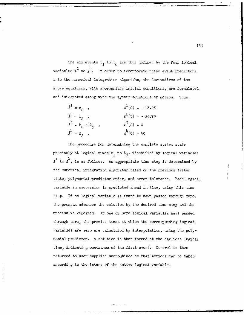
153
The six events t to t6 are thus defined by the four logical
14
variables I to A . In order to incorporate these event predictors
into the numerical integration algorithm, the derivatives of the
above equations, with appropriate initial conditions, are formulated
and integrated along with the system equations of motion. Thus,
l =k 2 , 1 (o) = -18.26
.2 2= k 2 A (0) = - 20.75
A3 = x 2 - 3 3 (0) 0
.4 =K2 4 (o) 4o
The procedure for determining the complete system state
precisely at logical times t1 to t6, identified by logical variables
1 41 to I , is as follows. An appropriate time step is determined by
the numerical integration algorithm based on the previous system
state, polynomial predictor order, and error tolerance. Each logical
variable in succession is predicted ahead in time, using this time
step. If no logical variable is found to have passed through zero,
the program advances the solution by the desired time step and the
process is repeated. If one or more logical variables have passed
through zero, the precise times at which the corresponding logical
variables are zero are calculated by interpolation, using the poly-
nomial predictor. A solution is then forced at the earliest logical
time, indicating occurance of the first event. Control is then
returned to user supplied subroutines so that actions can be taken
according to the intent of the active logical variable.

!
154
Discontinuous events can be categorized according to the order
of increasing difficulty as follows:
(1) Those requiring restart of the integration process only,
such as when discontinuous forces act on or within the
system. These forces are not considered to be impulsive
in nature, thus only discontinuous accelerations result.
(2) Those requiring momentum balance due to impulsive external
loads (impact between bodies and mass capture or release
is excluded) with no supplemental restitution equations
or constraint equation modification.
(3) Those requiring momentum balance due to impact between
bodies and mass capture or release. Supplemental
coefficient of restitution equations are appended to the
momentum balance equations to achieve the desired
velocity changes. Constraints are added or deleted, as
needed to facilitate mass capture or release.
The six events t to t6 fall into the following three
categories:
(1) tl, t 3 , t5 - These events define discontinuous forces of
relatively small magnitude, therefore only a restart of
the integration procedure is required.
(2) t 2 - This event defines an externally applied impulsive
load requiring a momentum balance and restart of the
integration procedure.

155
(3) t4, t6 - These events define impulsive loading, due to
impact between bodies of the system, and mass capture and
release. Supplemental equations are required for momentum
balance and a restart of the integration procedure is
required.
The effects of the various events at logical times t to t6
on the position, velocity, and acceleration of the barrel are shown
in Figures 6.27 to 6.29, respectively.
The logical events are clearly marked by discontinuities in
acceleration of the gun tube as shown in Figure 6.29. At t2, an
impulse of - 880 lb f-sec is applied to the barrel, resulting in a
discontinuity in velocity and a change in barrel direction. The
applied loads are changed at this instant, resulting in a net change
in acceleration.
Impact between barrel and sear occurs at t4 , resulting in a
second discontinuity in barrel velocity. Buffer action on the
combined sear and barrel mass results in an acceleration of
4500 in/sec 2 in the time interval t 4 to t5. The dynamic response
curves of Figures 6.28 and 6.29 clearly indicate the intermittent
nature of weapon mechanism motion. It is emphasized that one
standard set of equations of motion and one standard set of momentum
balance equations are generated by the program. At the various
logical times, one simply appends or removes constraints, restitution
equations, forces, impulses, etc., as directed by programmed control
., w n -.-. - - .. n- -mi am m mm m unll m nniNnn

-156
-Sp
00
4J,
4, 0
02
4, 4J
0 02
0) q~l 4uu0)~dT

157
44-)
C)
4~j
'd 0ti

158
Lo~
4-)
C4--
Cuossqu)U~vaac

I
159
logic, determined by the active logical variables. Thus, an entire
simulation can be completed in a single computer run.
......

16o
CHAPTER 7
CONCLUSIONS AND RECOMMENDATIONS
7.1 Conclusions
In this report, two methods are presented to improve efficiency
of a general purpose dynamic analysis and design system computer
program. The first method employs Gaussian elimination in the con-
straint Jacobian matrix to identify independent and dependent
generalized coordinates, thus defining a minimal set of differential
equations whose solution yields total system response. The second
method employs pieced interval analysis with a logical events monitor
and momentum balance capability to efficiently handle intermittent
motion problems.
The analysis techniques have demonstrated an order of magni-
tude improvement in program performance. Since these methods require
no change in equation formulation, generality of the program is
maintained.
The methods developed are effectively applied to kinematic,
kinetostatic, and dynamic analysis of constrained planar and three-
dimensional systems. In addition, current investigations have
demonstrated that performance of an analysis program that includes
body flexibility is significantly improved when a minimum number of
equations of motion are solved.

161
7.2 Recommendations
The method of coordinate partitioning has potential in
other areas where coordinates are related by algebraic constraint
equations. For example, Heltne [59] makes the following statements
in his thesis when discussing techniques for solving large-scale
nonlinear programming problems:
(1) "Luenberger [60] in his proof of the convergence rate
of the GRG algorithm [59 ] shows this convergence rate to be
coordinate dependent. That is, the convergence rate is a function
of which variables are selected to be basic (dependent) and which
nonbasic (independent)."
(2) "A second theoretical problem is the use of (matrix)
structural considerations for selecting the basis. For example, the
use of a relation such as maximizing the trace or the product of the
diagonal elements of a matrix."
He further states that, "a nonzero diagonal does not imply a
nonsingular matrix, but some relation based upon the elements of the
Jacobian matrix may be a feasible alternative."
The method of Gaussian elimination with full row and column
pivoting for coordinate partitioning accomplishes all of the above
requirements. Furthermore, as discussed in Chapter 3, the resulting
matrix will generally have the largest determinant of all possible
submatrices, it will generally be well conditioned, and it has the
largest elements on the diagonal.

162
The coordinate partitioning method has pitfalls when the
constraint Jacobian matrix is sparse. To maintain program efficiency
sparse matrix algorithms employ a partial pivoting strategy that
generally does not select the largest pivotal elements. Thus,
coordinate partitioning by this method will not be optimum. This
may cause problems when attempting to maintain error control on
dependent variables.
The approach taken in this study is to periodically construct
a full matrix version of the constraint Jacobian and factor using
the algorithm of Appendix A. This step, requiring O(r3 ) operations
and m x 3n memory locations, is undesirable for large sparse systems.
Following this, the sparse matrix is then augnented to force zero
changes in independent variables at each iteration step. When
systems experience large angular displacements the independent
variable set changes frequently and correspondingly the sparse matrix
structure changes. Costly symbolic sparse matrix refactorization
are then required [61 3.
Heltne [ 59 ] has recently developed sparse matrix manipulation
algorithms employing block lower triangular factorization. This
technique is also employed by the sparse matrix code in DADS.
However, he has further developed an algorithm for ordering
matrices after a rank-one update. That is, when the matrix has been
put into block lower triangular form and the independent and dependent
sets change, generally a new symbolic factorization can be obtained
at a fraction of the cost of a complete matrix refactorization. He

163
has demonstrated an order of magnitude reduction in computer cost.
When the variable sets change often, which is the case when bodies
experience large angular displacements, the savings will be signif-
icant.
Additional research required in this and related areas is:
(1) Investigate the most efficient methods of Gaussian
elimination employing sparse matrix techniques solely
for the purpose of identifying optimum coordinate
partitioning, thus eliminating full matrix factorization.
(2) Implement Heltne's matrix ordering rank-one update
algorithm into the sparse matrix code.
(3) Investigate methods for determining when Gaussian
elimination is required for the purpose of redetermining
the partitioning of variables into dependent and inde-
pendent sets.
(4) Investigate methods of analyzing coordinate velocities
and accelerations as an alternate procedure for deter-
mining the need for applying Gaussian elimination in 3.
Or as a complete replacement for 3. One such technique
might be to compare differences between extrapolated
dependent variables (provided by the integration
algorithm) and the corrected dependent variables (pro-
vided by Newton iteration to satisfy constraints). A
large discrepancy between a predicted and a corrected
dependent variable is an indication that it should become

164
independent. Correspondingly an independent variable
having a reduced or minimum velocity and an acceleration
indicating that it may remain small for some time should
then be made dependent. The reverse process of looking
at maximum dependent velocity and corresponding accel-
eration could also be employed to identify a variable
for the independent set.
(5) Investigate methods for relating constraint closure
tolerance to numerical integration error tolerance.
Tight constraint tolerance results in excessive Newton
iterations with no gain in accuracy. Loose constraint
tolerance results in poor dependent variable prediction
which again results in additional corrector iterations
or excessive dependent variable error. Methods that
dynamically adjust constraint tolerance to minimize the
number of corrector iterations should be investigated.

165
APPENDIX A
RANK DETERMINATION AND DECOMPOSITION
OF SINGULAR MATRICES
A.1 Introduction
The technique and basic structure of the subprogram described
here are patterned after the subroutine MGR of the Scientific
Subroutine Package, an IBM application program [ 22]. Consider a
system of equations of the form
A(m x n) ' X(n x 1 ) = b(m X l) (A.l)
where in general the matrix A may lack full row and/or column rank.
The task is to determine if one or more solutions to Equation A.1
exist, and to find at least one efficiently and accurately.
The following calculations can be performed on a general rec-
tangular matrix which allows one to obtain solutions to Equation A.1
if such exist:
(1) Determine matrix rank and linearly independent rows and
columns.
(2) Express a submatrix of maximal rank, as a product of
triangular factors.

166
(3) Express nonbasic rows in terms of basic rows.
(4) Express basic variables in terms of free variables.
A.2 Theoretical Background
Basic variables, taken here as dependent variables, will be
denoted by the vector u and free variables, taken as independent
variables, will be denoted by the vector v.
Calculation (1) is most critical. Matrix rank is determined
using the standard Gaussian elimination technique, with complete
pivoting. Therefore, the rows and columns of the m by n matrix A
are generally interchanged at each elimination step to bring the
largest element to the pivot position. The interchange information
is recorded in two integer permutation vectors IROW and ICOL.: The
•thi row (column) of the interchanged matrix corresponds to the IROW
(I) th row (ICOL (I)th column) in the original matrix A. Initially,
IROW(J) = J and ICOL(J) = J.
The notation Ai is used for the interchanged matrix implied
at the ith elimination step. Superscripts do not mean powers. They
indicate the current elimination step at which the result is obtained.
A.2.a First Elimination Step
Let ajk be the absolutely greatest element of matrix A, which
is found firrt in a columnwise scan. The internal tolerance TOL is
set equal to IEPS - aJki. The parameter EPS is a specified error
level whose magnitude should be of the order of the existing computer
round off error level.

167
If ja kl< TOL, further calculation is bypassed. Otherwise
rows 1 and j and columns 1 and k of matrix A are interchanged, giving
1A . The same interchanges must be applied to TROW, interpreted as a
column vector, and to ICOL, interpreted as a row vector.
A is uniquely expressed as the product L • D • U by
imposing the following conditions:
(I) L1 is the m by m identity matrix, except for the first
column. The first diagonal element has a value of one.
(II) D is an m by n matrix with first diagonal element equal
to one, while all remaining elements of the first row and
column are equal to zero.
(III) Ul is the n by n identity matrix, except for the first
row.
21 1 1
1 L . D1 . UI
ML t D
More explicitly,

168
1 1a = U1
1 -A12 12
(A.2)1 1 :1
A = L U21 21 11
1 1 1 + 122 21 12 22
Capital le- ers are used as notation for matrices in this
appendix. Small letters represent scaler or vector quantities. The
symbol 0 means zero matrices and I means identity matrices, where
dimensions are implied by compatibility. The terms in Equation A.2
are further described as follows:
The elements of the first column of L1 are
1 1 1 .. 1 = 1 1
1ii = 1 21 = a21 /all' " ml aml/all
1 1fDThe elements of submatrix D of D are
22
1 11 1 1i 1 a *a
ik Aik il k ik 1al1 k =2, ..., n
The elements of the first row of U9 are
2. 1 1 1 1 1U1l1 a1l, u12 =a 1 2, ..., Uln =aln

169
Note that iL is possible to record all nontrivial cntri., uP I I)1
and Ul compactly in the storage locations occupied by the original A,
storing only:
A.2.b. Second Elimination Step
Let d1 j _ 2 be the absolutely largest element of D2 2 . ifjk', k 5 222
Idk1 TOL, D is interpreted as being the zero matrix.
If D is not zero in the above sense, it may be decomposed22P
analogously. In the compact scheme of above, rows 2 and j, and columns
2 and k are interchanged, obtaining
U1l Ui2
L21 D22
The same interchanges must be performed with IROW (interpreted as a
column vector), with ICOL (interpreted as a row vector), and with A1
giving

170
A2 = 1 01 ULU22 112
L 21 1 D22I
Now D22 may be expressed uniquely as the product of the form L*DU,22
imposing conditions I, II, and III. The result is
Then A2 L 2 D2 U2, with
1 0 0
2 2
21 21
2 2
L- L
21 L32
1 0 0
21
D = 0 1
220 0 D2

A
171
1 2 2U11 u12 U13
2 2 2= 0 u2 2 U2 3
0 0 I
where
2 2 2 221 LLlI ' U1 2 = 12' U 13
A.2.c. Final Result of Elimination Process2
At the next elimination step D is factorized, and so on.33
Now assume that finally r r equals zero in the sense that all
its elements are absolutely less than TOL. This means that A has
the rank r and the end result is the factorization Ar = Lr Dr ;
that is,
1 0 ... 0 0
221 1 . 0 0
Ar=
r r • 1 0rl r2 '"
r+l,l L .. Lr IL l r+l,2* r+l,r -
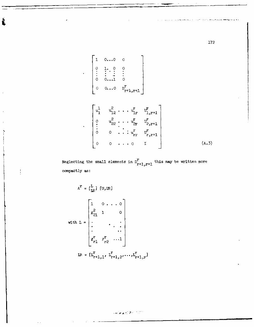
172
1 O...0 0
o 1. 0 0
o o ... 0
0 0...I Dr
L. 0 Dr+l,r+l
1 2 r .)1 12 " ir l,r+l
2 r0 u2 . . U r-22 2r 2,r+l
0 r urS 0 Urr r,r+l
o 0 • • (A.3)
Neglecting the small elements in Dr this may be written morer+l,r+1
compactly as:
Ar L I[,RA= [U] [u,UR]
1 0... 0
2A21 1 0
with L=
r rri r2
R Lr r r[r+l r+1,2 "'''Lr+l,r
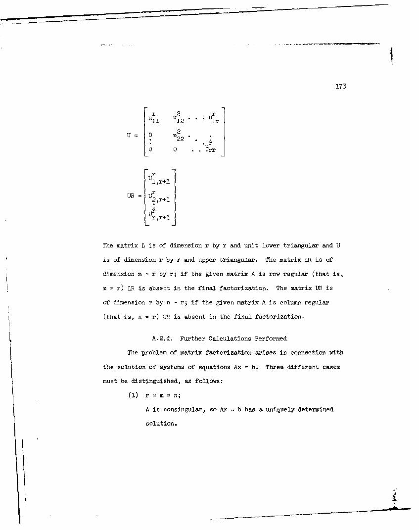
173
1l U2 r
~]
U ,rl220 0 . . .r
r,r+l
The matrix L is of dimension r by r and unit lower triangular and U
is of dimension r by r and upper triangular. The matrix LR is of
dimension m - r by r; if the given matrix A is row regular (that is,
m = r) LR is absent in the final factorization. The matrix UR is
of dimension r by n - r; if the given matrix A is column regular
(that is, n r) UR is absent in the final factorization.
A.2. d. Further Calculations Performed
The problem of matrix factorization arises in connection with
the solution of systems of equations Ax = b. Three different cases
must be distinguished, as follows:
() r = m = n;
A is nonsingular, so Ax = b has a uniquely determined
solution.

174
(2) r < m;
A is not row regular, so solutions of Ax b exist only
if linear combinations among the rows of A are also valid
among the rows of b
(3) r < n;
A is not column regular, so Ax = 0 has nontrivial
solutions.
The cases (2) and (3) may occur combined.
The solution, if it exists, is uniquely determined if r = n.
Otherwise, it contains n - r free parameters. Often one requires the
linear combinations among the rows of a given matrix A and the linear
forms expressing basic variables in terms of free ones. Therefore,
instead of LR and UR, matrices C and H are returned, containing
linear combinations and homogeneous solutions respectively.
Observe that the above calculated factorization belongs to the
interchanged matrix Ar . Therefore, Arxr = br is dealt with instead] i x~1 CICOL(I) thI
of Ax = b, where [b r ist obtained from [b] , using the I OL(j)thIbr th bIROW(J) th
element of [b] as the jhI element of
br J ,.
r rbILet xr , b be partitioned into [u] and 2]. Then,
b 1 b
II u, URI ] ~ 21• 1),

- 7
I175
or explicity,
L * U u + L UR v =b
LR * U u + LR • UR • v = b2
Since L and U are nonsingular, this implies that
= U-1 L-1 bI -UluU L. .b . . UR •v
LR L l b b 2
For convenience, LR is replaced by LR L- = C and UR is
replaced by - U-1 • UR = H, while L and U remain untouched. Consis-
tency requires that b 2 = C • b , and homogeneous solutions are given
by u = H * v. In case of a consistent system of equations Ar - xr
br, the general solution is xr = [u], with u = U-1 . L-1 bI1 + H
v, while the values of the free variables contained in v may be
chosen arbitrarily.
A.2.e. Format of Results
The subprogram returns matrices L, U, C, H, and D in the
storage area originally occupied by the input matrix A, in the com-
pact scheme shown in Figure A.l.
__ _ _ _ __ _ _ _ __ _ _

176
~n
L H
C D
Figure A.1. Format scheme of the processed matrix.

177
REFERENCES
1. Hrones, J. A. and Nelson, G. L., Analayis of the Four-BarLa, Technology Press of M.I.T., Cambridge, MA, and Wiley,New York, NY, 1951.
2. Artobolevskii, I. I., Meehanj sms for the Generation of Plane9 , (trans. by R. D. Wills), Macmillan, New York, NY, 1964.
3. General Motors, "GMR DYANA" Programming Manuals I and II-GMR 229 and GMR 237, Research Laboratories, G. M. Corp., Detroit,MI, 1959.
4. Korn, G. A. and Korn, T. M., Electronin Analna and HybridCo t , McGraw-Hill, Inc., New York, NY, 1964.
5. Okuno, S., Simulation of Motor Scra-ner Overturns, Ph.D. disser-tation, Cornell University, August, 1977.
6. Davis, D., Simulation and Model Verification of AEriculturalTractor Overturns, Ph.D. dissertation, Cornell University, 1973.
7. Paul, B. and Krajcinovic, D., "Computer Analysis of MachinesWith Planar Motion--Part I: Kinematic; Part II: Dynamics",ASME Journal of Apnplie& Mechanics, SerE, Val, 37, 697-712,1970.
8. Chace, M. A. and Smith, D. A., DAMN-A Digital Computer Progranfor the Dynamic Analysis of Generalized Mechanical Systems, SAEpaper 710244, January, 1971.
9. Sheth, P. N. and Uicker, J. J., Jr., "IMP (Integrated MechanismsProgram), A Computer Aided Design Analysis System for Mechanismsand Linkages" ASME Journal of Engineering for Industry, Ser. B,2LA 454-464, 1972.
10. Orlandea, N., Chace, M. A., and Calahan, D. A., "A Sparsity-Oriented Approach to the Dynamic Analysis and Design ofMechanical Systems, Parts I and II", ASME Journal of Engineeringfor.J Inus ., Ser. B, Val, .9, 773-784, 1977.
11. Langrana, N. A. and Bartel, D. L., "An Automated Method forDynamic Analysis of Spatial Linkages for Biomedical Applications",
I;

178
ASME Journal of Engineering for Induatry, § Vl,7 No. 2,566-574, 1975.
12. Rogers, R. J. and Andrews, G. C., "The Simulation of Plan&Systems Using a Simplified Vector-Network Method", MAn ±Aand Machine Theory, Vol. 10, 509-519, 1975.
13. Liegois, A., Khalil, W., and Dumas, J. M., "Mathematical andComputer Models of Interconnected Mechanical Systems", Prngd-inas of the Symposium on Theory and Practice of Robots andM, Warsaw, Poland, September, 1976.
14. Williams, R. J. and Seireg, A., "Interactive Modeling andAnalysis of Open or Closed Loop Dynamic Systems With RedundantActuators", ASME Journal of Mechanical Desian, Vol. iO1, 407-416, July, 1979.
15. Paul, B., Kine-iatica an Dynel ics of Planar Mac~hnery, Prentice-Hall, Inc., Englewood Cliffs, NJ, 1979.
16. Sheth, P. N., A Digltal Conmgter Baned SimiLation Procedure forMultinle Desree of Freedom Mechanical Systems with GecnetricC i , Ph.D. dissertation, University of Wisconsin, 1972.
17. Smith, D. A., Reaction Forces and Imact in Generalized Two-Dimensional Mechanical Dynamic Systems, Ph.D. dissertation, TheUniversity of Michigan, 1971.
18. Shampine, L. F., Watts, H. A. and Davenport, S. M., "SolvingNonstiff Ordinary Differential Equations - the State of theArt", S, Vol. 18, No. 3, 376-411, July, 1976.
19. Orlandea N., Node Analngous, Sparsit-Oriented Methods forSimalation of Mechanical Dynamigc Systems, Ph.D. dissertation,The University of Michigan, 1973.
20. Gear, C. W., "Simultaneous Numerical Solution of Differential-Algebraic Equations", IEEE TransUations on Circuit Thearyg,Vol. a-4, No. 1, 89-95, January, 1971.
21. Haug, E. J. Wehage, R. A., and Barman, N. C., "Design Sensi-tivity Analysis of Planar Mechsnism and Machine Dynamics", toappear in ASNE Jnurnsl of Mehanca! Desiam.
22. SV,, ., ml36, S gi ni-fi S,,har.ut11a P &C W (36 QA-CM-O 3X),
22. a n U

179
23. Orlandea, N., Wiley, J. C. and Wehage, R. A., ADAMS2: A SparseMatrix Approach to the Dynamic Simulation of Two-DimcnsionalMechaical Systems, Society of Automotive F.ngineers TechnicalPaper Series 780486, 1978.
24. Nikravesh, P. E. and Chung, I. S., "Application of Euler Para-meters to the Dynamic Analysis of Three Dimensional ConstrainedMechanical Systems - A General Purpose Computer Program",submitted to ASME Journal of Mechanical Design.
25. Song, J. 0. and Haug, E. J., "Dynamic Analysis of FlexibleMechanisms", to appear in Comuter Methods in Applied Mechanicsand Enineering.
26. Chao, E. Y. and Rim, K., "Application of Optimization Principlesin Determining the Applied Moments in Human Leg Joints DuringGait", Journal of Biomechanics, Vol, 6, 497-510, 1973.
27. Szidarovszky, F. and Yakowitz, S., Principles and Procedures ofNumerical Analysis, Plenum Press, 227 West 17th Street, NewYork, NY.
28. Shampine, L. F. and Gordon, M. K., Computer Solution of OrdinaryDifferential Equations: The Initial Value Problem, W. J.Freeman, San Francisco, CA, 1975.
29. Carver, M. B., "Efficient Integration Over Discontinuities inOrdinary Differential Equation Simulations", Mathematics AndCommuters in Simuationlo, P0 190-196, 1978.
30. Dugas, R., A History of Mechanics. Editions du Gri-fon,Neuchatel-Switzerland, 1955.
31. van Bokhoven, W. M. G., "Linear Implicit DifferentiationFormulas of Variable Step and Order", IEEE Transactions onCircuits and Systems, CAS-22, No. 2, 109-115, February, 1975.
32. Duff, I. S., MA28-A Set of FORTRAN Subroutines for SnairseUnsvmmetric Linear Equations, Report No. AERE-R.8730, ComputerScience and Systems Division, AERE Harwell, Oxfordshire, July,1977.
33. Greenwood, D. T., Princples of Dynamics, Prentice-Hall,
Englewood Cliffs, NJ, 1965.
34. Haug, E. J. and Arora, J. S., Annpled Optimnal Des!gn, John Wileyand Sons, New York, NY, 1979.

180
35. Chua, L. 0. and Lin, P. M., Cout_-Adfc1 Analamil ofElectroni Cirmuita: Alhorithin and Cammutational Techninues,Prentice-Hall, Inc., Englewood Cliffs, NJ, 1975.
36. Gear, C. W., Nmeripal Initial Value Problems in OrdinaryDifferential Equations, Prentice-Hall, Inc., Englewood Cliffs,NJ, 1971.
37. Brameller, A., Allen, R. N., and Hamen, Y. M., Sa , PitmanPublishing Corporation, New York, NY, 1976.
38. Friend, J. H., Guralnik, D. B., et al., Webnter's New WorldDictionar= of the American Language, College Edition, TheWorld Publishing Company, Cleveland, OH, 1959.
39. Wells, D. A., Sh-'s Outline of Theory and Problems ofLagrangian Dyamics, McGraw-Hill Book Co., St. Louis, MO, 1967.
40. Sheth, P. N., Improved Iterative Techniques for the (4 ;c 4)Matrix Method of Kinematic Analysis, M. S. dissertation,University of Wisconsin, 1968.
41. Forsythe, G. E. and Moler, C. B., Computer Solution of LinearAlgebratc Systems, Prentice-Hall, Englewood Cliffs, NJ, 1967.
42. Paul, B., "Analytical Dynamics of Mechanisms--A ComputerOriented Overview", Mechanism and Machine Theory, Vo .,_0, 481-507, 1975.
43. Huang, R. C., Haug, E. J. and Andrews, J. G., "SensitivityAnalysis and Otimal Design of a Mechanical System with Inter-mittent Motion , ASME Journal of Mechanica Design, YL.Q.,492-499, 1978.
44. Nordsieck, A., "Automatic Numerical Integration of OrdinaryDifferential Equations", Proceedinan of Sympoaium on Ayplied
SVol, 1, 241-250, 1963.
45. Brayton, R. K., Gustavson, F. G., and Hachtel, G. D., "A NewEfficient Algorithm for Solving Differential-Algebraic SystemsUsing Implicit-Backward Differential Formulas", PE fj.na LtheLEEE, Vol. 60, No. 1, 98-108, January, 1972.
46. Calahan, D. A. and Orlandea, N., "A Program for the Analysis andDesign of General Dynamic Mechanical Systems", AFIPS ConferenceP, VW., Part II, 885-888, 1972.

181
47. Beck, R. R. and Kamnm, I. 0., Cybernetically Coupled ResearchVehicle, Society of Automotive Engineers, Rep. 75-217, February,1975.
48. Kainm, 1. 0. and Beck, R. R., The Performance of the CoupledM-113 Armored Personnel Carriers, 5th International Conference,Detroit, Michigan, International Society for Terrain-VehicleSystems, June, 1975.
49. Conte, S. D. and de Boor, C., Elementary Numerical Analysis anAlaorithmic Aopuroach, McGraw-Hill Book Co., St. Louis, MO, 1972.
50. Vandergraft, J. S.., Introduction to Numerical Computations,Academic Press, New York, NY, 1978.
51. Vehicle platform stability analysis being performed for theU. S. Army TARADCOM.
52. Hoogterp, F. B., Digital/Analon Vehicle Ride Simulation,Technical Report No. 11705, U. S. Army Tank Automotive Command,Warren, MI, November, 1972.
53. Beck, R. R. and Wehage, R. A., "The Modeling and Simulation ofTwo Coupled M-113 Armored Personnel Carriers", Proceedinas ofthe Tenth Annual Pittsburgh Conference on Modeling and Simula-tion, Vol, 10, Part 2, 353-359, 1979.
54. Ehle, P. E. and Haug, E. J., "A Logical Function Method forDynamic and Design Sensitivity Analysis of Mechanical Systemswith Intermittent Motion", to appear in ASME Journal ofMechanical Desian.
55. Kecs, W. and Teodorescu, P. P., Apnlications of the Theory ofDistributions in Mechanics, Abacus Press, Tunbridge Wells,Kent, England, 1974.
56. Huang, R. C. and Haug, E. J., "A Distribution Theoretic Methodfor Design Sensitivity Analysis of Mechanisms with IntermittentMotion; Part I: Theory; Part II: Applications", DinMe n , Proceedings of the 16th Midwestern MechanicsCofrec, Vol, 10, 115-126, 1979.
57. Ehle, P. E., Dynamic Analysis and Desigm Sensitivity Analysisof Mechanisms with Intermittent Motion, Technical Report No. 48,Division of Materials Engineering, College of Engineering, TheUniversity of Iowa, February, 1979.

182
58. Wehage, R. A. and Haug, E. J., "Generalized Coordinate Parti-tioning for Dimension Reduction in Analysis of ConstrainedDynamic Systems", to appear in the ASME Journal of Mechanical
59. Heltne, D. R., Nonlinear Pro&ramming in Chemical EngineeringDi, Ph.D. dissertation, The University of Iowa, 1979.
60. Luenberger, D. G., Introduction to Linear and NonlinearProarwming, Addison-Wesley, Reading, MA, 1973.
61. Reid, J. K., Sparse Matrices, C. S. S. 31, Presented at theIMA Conference, "The State-of-the-Art in Numerical Analysis",York, April 1976, Computer Science and Systems Division, A. E.R. E., Harwell, Didcot, Oxen, May, 1976.

DISTRIBUTION LIST
Please notify USATACOM, DRSTA-ZSA, Warren, Michigan 48090, of corrections
and/or changes in address.
Commander . (25) Director (31)
US Army Tk-Autmv Command Defense Advanced ResearchR&D Center Projects AgencyWarren, MI 48090 1400 Wilson Boulevard
Arlington, VA 22209Superintendent (02)US Military Academy Commander (01)ATTN: Dept of Engineering US Army Combined Arms Combat
Course Director for Developments ActivityAutomotive Engineering ATTN: ATCA-CCC-S
Fort Leavenworth, KA 66027
Commander (01)US Army Logistic Center Commander (01)
Fort Lee, VA 23801 US Army Mobility EquipmentResearch and Development Command
US Army Research Office (02) ATTN: DRDME-RTP.O. Box 12211 Fort Belvoir, VA 22060ATTN: Dr. F. Schmiedeshoff
Dr. R. Singleton Director (02)
Research Triangle Park, NC 27709 US Army Corps of EngineersWaterways Experiment Station
HO, DA (01) P.O. Box 631
ATTN: DAMA-AR Vicksburg, MS 39180
Dr. HerschnerWashington, D.C. 2031C Commander (01)
US Army Materials and Mechanics
HQ, DA (01) Research CenterOffice of Dep Chief of Staff ATTN: Mr. Adachi
for Rsch, Dev & Acquisition Watertown, MA 02172
ATTN: DAMA-ARDr. Charles Church Director (03)
Washington, D.C. 20310 US Army Corps of EngineersWaterways Experiment Station
HO, DARCOM P.O. Box 631
5001 Eisenhower Ave. ATTN: Mr. NuttallATTN: DRCDE Vicksburg, MS 39180
Dr. R.L. HaleyAlexandria, VA 22333 Director (04)
US Army Cold Regions Research
& Engineering LabP.O. Box 282ATTN: Dr. Freitag, Dr. W. HarrisonDr. Liston, Library
Hanover, NH 03755

President (02) Director (02)Army Armor and Engineer Board Defense Documentation CenterFort Knox, KY 40121 Cameron Station
Alexandria, VA 22314Commander (01)US Army Arctic Test Center US Marine Corps (01)APO 409 Mobility & Logistics DivisionSeattle, WA 98733 Development and Ed Command
ATTN: Mr. HicksonCommander (02) Quantico, VA 22134US Army Test & EvaluationCommand Keweenaw Field Station (01)ATTN: AMSTE-BB and AMSTE-TA Keweenaw Research CenterAberdeen Proving Ground, MD Rural Route 121005 P.C. Box 94-D
ATTN: Dr. Sung M. LeeCommander (01) Calumet, MI 49913US Army Armament Researchand Development Command Naval Ship Research & (02)ATTN: Mr. Rubin Dev CenterDover, NJ 07801 Aviation & Surface Effects Dept
Code 161Commander (01) Washington, D.C. 20034US Army Yuma Proving GroundATTN: STEYP-RPT Director (01)Yuma, AZ 85364 National Tillage Machinery Lab
Box 792Commander (01) Auburn, AL 36830US Army Natic LaboratoriesATTN: Technical Library Director (02)Natick, MA 01760 USDA Forest Service Equipment
Development CenterDirector (01) 444 East Bonita AvenueUS Army Human Engineering Lab San Dimes, CA 914773ATTN: Mr. EckelsAberdeen Proving Ground, MD Engineering Societies (01)21005 Library
345 East 47th StreetDirector (02) New York, NY 10017US Army Ballistic Research LabAberdeen Proving Ground, MD Dr. I.R. Erlich (01)21005 Dean for Research
Stevens Institute of TechnologyDirector (02) Castle Point StationUS Army Materiel Systems Hoboken, NJ 07030Analysis AgencyATTN: AMXSY-CMAberdeen Proving Ground, MD21005

Grumman Aerospace Corp (02) CALSPAN Corporation (01)South Oyster Bay Road Box 235ATTN: Dr. L. Karafiath Library
Mr. F. Markow 4455 Benesse StreetM/S A08/35 Buffalo, NY 14221
Bethpage, NY 11714SEM, (01)
Dr. Bruce Liljedahl (01) ForsvaretsforskningsanstaltAgricultural Engineering Dept Avd 2
Purdue University Stockholm 80, SwedenLafayette, IN 46207
Mr. Hedwig (02)Mr. H.C. Hodges (01) RU 111/6Nevada Automotive Test Center Ministry of DefenseBox 234 5300 Bonn, GermanyCarson City, NV 89701
Foreign Science & Tech (01)Mr. R.S. Wismer (01) Center
Deere & Company 220 7th Street North EastEngineering Research ATTN: AMXST-GEI3300 River Drive Mr. Tim NixMoline, IL 61265 Charlottesville, VA 22901
Oregon State University (01) General Research Corp (01)
Library 7655 Old Springhouse RoadCorvallis, OR 97331 Westgate Research Park
ATTN: Mr. A. ViiiuSouthwest Research Inst (01) McLean, VA 221018500 Culebra RoadSan Antonia, TX 78228 Commander (01)
US Army Developmant andFMC Corporation (01) Readiness CommandTechnical Library 5001 Eisenhower AvenueP.O. Box 1201 ATTN: Dr. R.S. WisemanSan Jose, CA 95108 Alexandria, VA 22333
Mr. J. Appelblatt (01)
Director of EngineeringCadillac Gauge Company
P.O. Box 1027Warren, MI 48090
Chrysler Corporation (02)Mobility Research Laboratory,Defense EngineeringDepartment 6100P.O. Box 751Detroit, MI 48231