ted:a Stata Command for Testing Stability of Regression

Discontinuity Models

Giovanni Cerulli

IRCrES, Research Institute on Sustainable Economic GrowthNational Research Council of Italy

2016 Stata ConferenceChicago, Illinois

July 28–29

1 / 41

Introduction

Given a running variable X , a threshold c , a treatment indicator T ,and an outcome Y , Regression Discontinuity (RD) models identifya local average treatment effect (LATE) by associating a jump inmean outcome with a jump in the probability of treatment T whenX crosses the threshold c .

Example: Jacob and Lefgren (2004): You are likely to be sent to summer school if

you fail a final exam. T indicates summer school, −X is test grade, −c is grade

needed to pass, Y is later academic performance.

2 / 41

Dong and Lewbel (2015) construct the Treatment Effect Derivative(TED) of estimated RD. TED is nonparametrically identified and easilyestimated.

They argue TED is useful because, under a local policy invarianceassumption, TED = MTTE (Marginal Threshold Treatment Effect).MTTE is the change in the RD treatment effect resulting from amarginal change in c .

We argue here that even without policy invariance, TED provides auseful measure of stability of RD estimates, in both sharp and fuzzyRD designs.

We also define a closely related concept, the CPD (Complier ProbabilityDerivative). We show that this is another useful measure of stabilityin fuzzy designs.

3 / 41

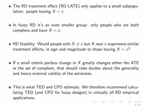
The RD treatment effect (RD LATE) only applies to a small subpopu-lation: people having X = c .

In fuzzy RD it’s an even smaller group: only people who are bothcompliers and have X = c .

RD Stability: Would people with X 6= c but X near c experience similartreatment effects, in sign and magnitude to those having X = c?

If a small ceteris paribus change in X greatly changes either the ATEor the set of compliers, that should raise doubts about the generalityand hence external validity of the estimates.

This is what TED and CPD estimate. We therefore recommend calcu-lating TED (and CPD for fuzzy designs) in virtually all RD empiricalapplications.

4 / 41

Angrist and Rokkanen (2015) recognize the issue. They estimate LATE awayfrom the cutoff, but require a strong running variable conditional exogeneityassumption.

In contrast, the only thing we impose to identify TED, beyond standard RDassumptions is additional smoothness: some differentiability (instead of justcontinuity) of potential outcome expectations.

Similar additional smoothness is already always imposed in practice - differ-entiability is included in the regularity assumptions needed for local regres-sions.

TED and CPD are trivial to estimate. In sharp designs TED equals acoefficient people were already estimating and throwing away, not knowingit was meaningful.

5 / 41

Literature Review

General RD identification and estimation: Thistlethwaite and Campbell(1960), Hahn, Todd, and van der Klaauw (2001), Porter (2003), Imbensand Lemieux (2008), Angrist and Pischke (2008), Imbens and Wooldridge(2009), Battistin, Brugiavini, Rettore, and Weber (2009), Lee and Lemieux(2010), many others.

RD derivatives: Card, Lee, Pei, and Weber (2012) regression kink designmodels (continuous kinked treatment). Dong (2014) shows standard RDmodels can be identified from a kink in probability of treatment. Slopechanges also used by Calonico, Cattaneo and Titiunik (2014).

Dinardo and Lee (2011) informal Taylor expansion at the threshold for ATT.

Policy invariance (outcome doesn’t depend on some features of the treat-ment assignment mechanism, a form of external validity) Abbring and Heck-man (2007), Heckman (2010), Carneiro, Heckman, and Vytlacil (2010).

6 / 41

Literature Review - continued

Sufficient assumptions and tests for RD validity: Hahn, Todd and Van derKlaauw (2001), Lee (2008), Dong (2016).

Almost all tests or analyses of internal or external validity of RD requirecovariates with certain properties: McCrary (2008), Angrist and Fernandez-Val (2013), Wing and Cook (2013), Bertanha and Imbens (2014), andAngrist and Rokkanen (2015).

TED and CPD do not require any covariates other than those used toestimate RD.

Identification and estimation of TED and CPD requires no additional dataor information beyond what is needed for standard RD models.

All that is needed for TED and CPD are slightly stronger smoothness conditions than for

standard RD. Similar required differentiability assumptions are already imposed in practice

when one uses local linear or quadratic estimators.7 / 41

Regression Discontinuity: Model Definitions

T is a treatment indicator: T = 1 if treated, T = 0 if untreated.example: Jacob and Lefgren (2004), T indicates going to summerschool.

Y is an outcome, e.g. academic performance in higher grades.

X is a running or forcing variable that affects T and may also affectY , e.g, −X is a final exam grade.

c is a threshold constant, e.g., −c is the grade needed to pass theexam.The RD instrument is Z = I (X ≥ c), e.g. Z = 1 if fail the exam,zero if pass it.

8 / 41

A ”complier” is an individual i who has Ti = 1 if and only if Zi = 1 (e.g. acomplier is one who goes to Summer school if and only if he fails the exam).

Sharp RD design: Everybody is a complier. The probability of treatment atX = c jumps from zero to one.

Fuzzy RD design: Some people are not compliers, e.g., teachers sometimesoverrule the exam results.

9 / 41

RD Model Treatment Effects

Average Treatment Effect, ATE: The average difference in outcomesacross people randomly assigned treatment (e.g. average increase inacademic performance Y if randomly chosen students switched fromnot attending to attending Summer school T ).

RD LATE denoted π (c): The ATE at X = c among compliers. (e.g.the ATE just among complier students at the borderline of passingor failing the exam).

The RD LATE is identified under very weak conditions by associatingthe jump in E (Y | X = c) with the jump in E (T | X = c).

RD Intuition: π can be identified at c , because for X near c as-signment to treatment is almost random. Assumes no manipulation:individuals can’t set X precisely.

10 / 41

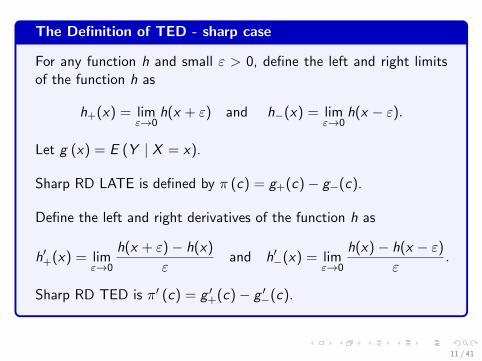
The Definition of TED - sharp case

For any function h and small ε > 0, define the left and right limitsof the function h as

h+(x) = limε→0

h(x + ε) and h−(x) = limε→0

h(x − ε).

Let g (x) = E (Y | X = x).

Sharp RD LATE is defined by π (c) = g+(c)− g−(c).

Define the left and right derivatives of the function h as

h′+(x) = limε→0

h(x + ε)− h(x)

εand h′−(x) = lim

ε→0

h(x)− h(x − ε)

ε.

Sharp RD TED is π′ (c) = g ′+(c)− g ′−(c).

11 / 41

The intuition behind TED - sharp case

Let Y = g0 (X ) + π (X )T + e.

e is an error term that embodies all heterogeneity across individuals.Endogeneity: X , T , and e may all be correlated.

π (x) is a LATE. Its the ATE among compliers having X = x .The treatment effect estimated by RD designs is π (c).

Let π′ (x) = ∂π(x)/∂x . TED is just π′ (c).

12 / 41

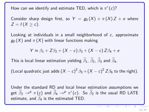
How can we identify and estimate TED, which is π′ (c)?

Consider sharp design first, so Y = g0 (X ) + π (X )Z + e whereZ = I (X ≥ c).

Looking at individuals in a small neighborhood of c , approximateg0 (X ) and π (X ) with linear functions making

Y ≈ β1 + Zβ2 + (X − c)β3 + (X − c)Zβ4 + e

This is local linear estimation yielding β̂1, β̂2, β̂3 and β̂4.

(Local quadratic just adds (X − c)2 β5 + (X − c)2 Zβ6 to the right).

Under the standard RD and local linear estimation assumptions weget β̂2 →p π (c) and β̂4 →p π′ (c). So β̂2 is the usual RD LATEestimate, and β̂4 is the estimated TED.

13 / 41

Fuzzy Design TED and CPD

For fuzzy design have two local linear (or local polynomial) regres-sions:

T ≈ α1 + Zα2 + (X − c)α3 + (X − c)Zα4 + u

Y ≈ β1 + Zβ2 + (X − c)β3 + (X − c)Zβ4 + e

First is the instrument equation, second is the reduced form outcomeequation.

First is local linear approximation of f (x) = E (T | X = x), secondis local approximation of g (x) = E (Y | X = x), recalling that Z =I (X ≥ c).

Recall a complier is one having T and Z be the same random variable.

14 / 41

T ≈ α1 + Zα2 + (X − c)α3 + (X − c)Zα4 + u

Y ≈ β1 + Zβ2 + (X − c)β3 + (X − c)Zβ4 + e

Let p (x) denote the conditional probability that someone is a com-plier, conditioning on that person having X = x . Let p′ (x) =∂p (x) /∂x .

By the same logic as in sharp design (replacing Y with T ), we have:

p (c) = f+(c)− f−(c) and p′ (c) = f ′+(c)− f ′−(c),

α̂2 →p p (c) and α̂4 →p p′ (c).

p′ (c) is what we call the CPD (Complier Probability Derivative),consistently estimated by α̂4.

15 / 41

T ≈ α1 + Zα2 + (X − c)α3 + (X − c)Zα4 + u

Y ≈ β1 + Zβ2 + (X − c)β3 + (X − c)Zβ4 + e

Let q (x) = E (Y (1) | X = x) − E (Y (0) | X = x), so q (c) =g+(c)− g−(c).

The fuzzy RD Late is πf (c) = q (c) /p (c), π̂f (c) = β̂2/α̂2.Applying the formula for the derivative of a ratio,

π′f (x) =∂πf (x)

∂x=∂ q(x)p(x)

∂x=

q′ (x)

p (x)−q (x) p′ (x)

p (x)2=

q′ (x)− πf (x)p′ (x)

p (x),

so the fuzzy design TED π′f (c) is consistently estimated by

π̂′f (c) =β̂4 − π̂f (c)α̂4

α̂2=β̂4 − (β̂2/α̂2)α̂4

α̂2

16 / 41

Stability

TED π′ (c) measures stability of the RD LATE, since π (c + ε) ≈π (c) + επ′ (c) for small ε.

Zero TED means π (c + ε) ∼= π (c), so individuals with x near c havealmost the same LATE as those with x = c .

Large TED means a small change in x away from c yields largechanges in LATE, i.e., instability.

17 / 41

Same stability argument holds for fuzzy designs, with πf (c + ε) ≈ πf (c)+επ′f (c).

π′f (c) = q′(c)p(c) −

q(c)p′(c)

p(c)2= q′(c)

p(c) −p′(c)πf (c)

p(c)

Fuzzy has two potential sources of instability. Fuzzy can be unstable because q′ (c)is far from zero or because p′ (c) is far from zero.

q′ (c) term large means the treatment effect for the average compiler changes alot as x moves away from c .

p′ (c) term large means that population of compliers changes a lot as x movesaway from c .

TED combines both effects.

CPD is just p′ (c).

18 / 41

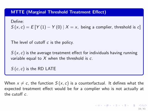
MTTE (Marginal Threshold Treatment Effect)

Define:S (x , c) = E [Y (1)− Y (0) | X = x , being a complier, threshold is c]

The level of cutoff c is the policy.

S (x , c) is the average treatment effect for individuals having runningvariable equal to X when the threshold is c .

S (c , c) is the RD LATE

When x 6= c , the function S (x , c) is a counterfactual. It defines what theexpected treatment effect would be for a complier who is not actually atthe cutoff c .

19 / 41

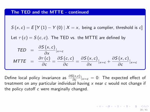
The TED and the MTTE - continued

S (x , c) = E [Y (1)− Y (0) | X = x , being a complier, threshold is c]

Let τ (c) = S (c , c). The TED vs. the MTTE are defined by

TED =∂S (x , c)

∂x|x=c

MTTE =∂τ (c)

∂c=∂S (c, c)

∂c=∂S (x , c)

∂x|x=c +

∂S (x , c)

∂c|x=c

Define local policy invariance as ∂S(x ,c)∂c |x=c = 0: The expected effect of

treatment on any particular individual having x near c would not change ifthe policy cutoff c were marginally changed.

20 / 41

If local policy invariance, then TED = MTTE. Given MTTE, wecan evaluate how the treatment effect would change if c marginallychanged.

If local policy invariance holds, then we estimate that the LATE wouldchange if the cutoff were changed.

Why might local policy invariance may fail to hold? General equilib-rium effects.

Example: in Jacob and Lefgren (2004) treatment is Summer school,the cutoff is an exam grade. Changing the cutoff grade would changethe size and composition of the Summer school student body possiblyaffecting outcomes.

21 / 41

Many policy debates center on whether to change thresholds. Examples:

Minimum wage levels.

Legal age for drinking, smoking, voting, medicare or pension eligibility.

Grade levels for promotions, graduation or scholarships.

Permitted levels of food additives or environmental pollutants.

...

A popular type of experiment is to compare outcomes before and after athreshold change. In contrast, we do not observe a change in the threshold,but MTTE still identifies what the effect would be of a (marginal) changein the threshold.

Even if local policy invariance fails, TED provides useful information for these

debates, by comprising a large component of the MTTE.

22 / 41

Stata implementation usingted

Cerulli, G., Dong, Y., Lewbel, A., and Paulsen, A. (forthcoming 2016), ”Testing Stability

of Regression Discontinuity Models”, Advances in Econometrics, Volume 38. Special

issue on ”Regression Discontinuity Designs: Theory and Applications”, Eds: Matias D.

Cattaneo (University of Michigan) and Juan-Carlos Escanciano (Indiana University).

23 / 41

Calonico, Cattaneo and Titiunik (2014): Robust Data-Driven Inference in

the Regression-Discontinuity Design, Stata Journal 14(4): 909-946.

24 / 41

Stata implementation using ted

25 / 41

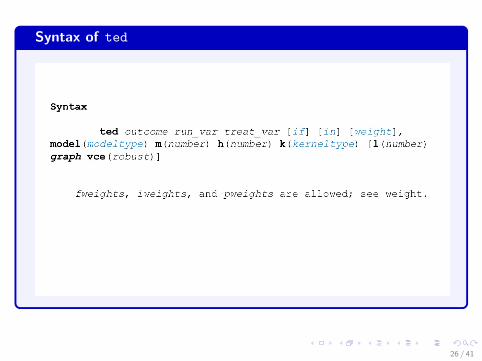
Syntax of ted

26 / 41

Options

27 / 41

Options - continued

28 / 41

Example 1: RDD-sharp

Ludwig and Miller (2007) assess the impact of the Head Start pro-gram.

Head Start was established in the United States in the year 1965. Itsobjective is to provide preschool, health, and other social services forpoor children ages three to five, as well as their families.

The 300 counties with the highest poverty rates received aid writinggrants, thus creating a large, persistent discontinuity in Head Startfunding.

Their main result focuses on Head Start funding’s effect on mortalitydue to causes Head Start should have an effect on, using povertyrates as their running variable.

29 / 41

Example 1: code for RDD-sharp

30 / 41

Example 1: ted output for RDD-sharp - 1

31 / 41

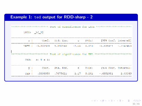
Example 1: ted output for RDD-sharp - 2

32 / 41

Example 1: ted output for RDD-sharp - 3

02

46

8O

utco

me

−6 6Running variable

Right local means Left local means

Tangent Prediction

Bandwidth type = Bandwidth value = KLPR = Kernel Local Polynomial RegressionPolynomial degree = 2Kernel = triangular

Fuzzy RD, KLPR, Outcome discontinuity

33 / 41

Example 2: RDD-fuzzy

We considers the fuzzy RD model in Clark and Martorell (2010,2014), which evaluates the signaling value of a high school diploma.

In about half of US states, high school students are required to passan exit exam to obtain a diploma. The random chance that leads tostudents falling on either side of threshold passing score generates acredible RD design.

Clark and Martorell takes advantage of the exit exam rule to eval-uate the impact on earnings of having a high school diploma.

The outcome Y is the present discounted value (PDV) of earningsthrough year 7 after one takes the last round of exit exams. Thetreatment T is whether a student receives a high school diploma ornot. The running variable X is the exit exam score (centered at thethreshold passing score).

34 / 41

Example 2: code for RDD-fuzzy

35 / 41

Example 2: ted output for RDD-fuzzy - 1

36 / 41

Example 2: ted output for RDD-fuzzy - 2

37 / 41

Example 2: ted output for RDD-fuzzy - 3

38 / 41

.2.4

.6.8

1P

roba

bilit

y of

a H

S D

iplo

ma

−20 −10 0 10 20Running variable

Right local means Left local means

Tangent Prediction

Bandwidth type = CCTBandwidth value = 17.24KLPR = Kernel Local Polynomial RegressionPolynomial degree = 2Kernel = triangular

Fuzzy RD, KLPR, Probability discontinuity

Figure: Fuzzy RD discontinuity in the probability and tangents lines at threshold.Dataset: Clark and Martorell (2010).

39 / 41

2600

030

000

Wag

es

−25 25Running variable

Right local means Left local means

Tangent Prediction

Bandwidth type = CCTBandwidth value = 17.24KLPR = Kernel Local Polynomial RegressionPolynomial degree = 2Kernel = triangular

Fuzzy RD, KLPR, Outcome discontinuity

Figure: Fuzzy RD discontinuity in the outcome and tangents lines at threshold.Dataset: Clark and Martorell (2010).

40 / 41

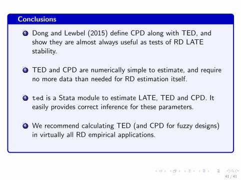
Conclusions

1 Dong and Lewbel (2015) define CPD along with TED, andshow they are almost always useful as tests of RD LATEstability.

2 TED and CPD are numerically simple to estimate, and requireno more data than needed for RD estimation itself.

3 ted is a Stata module to estimate LATE, TED and CPD. Iteasily provides correct inference for these parameters.

4 We recommend calculating TED (and CPD for fuzzy designs)in virtually all RD empirical applications.

41 / 41