technology technical note mo-3 - home | nrcs technical note mo-3 april 20, 2010 -12- the cell size...
TRANSCRIPT
April 20, 2010
Technology Technical Note MO-3
LiDAR USER’S GUIDE for ArcMap 9.2

Technology Technical Note MO-3 LiDAR User’s Guide for ArcMap 9.2 April 20, 2010 Prepared by: Unites States Department of Agriculture Natural Resources Conservation Service Missouri State Office 601 Business Loop 70 West, Suite 250 Columbia, Missouri 65203 www.nrcs.mo.usda.gov The U.S. Department of Agriculture (USDA) prohibits discrimination in all its programs and activities on the basis of race, color, national origin, age, disability, and where applicable, sex, marital status, familial status, parental status, religion, sexual orientation, genetic information, political beliefs, reprisal, or because all or a part of an individual's income is derived from any public assistance program. (Not all prohibited bases apply to all programs.) Persons with disabilities who require alternative means for communication of program information (Braille, large print, audiotape, etc.) should contact USDA's TARGET Center at (202) 720-2600 (voice and TDD). To file a complaint of discrimination write to USDA, Director, Office of Civil Rights, 1400 Independence Avenue, S.W., Washington, D.C. 20250-9410 or call (800) 795-3272 (voice) or (202) 720-6382 (TDD). USDA is an equal opportunity provider and employer.

Technology Technical Note MO-3
i April 20, 2010
Table of Contents Page A. LiDAR Data Overview .......................................................................................... 1
B. Folder Structure .................................................................................................. 1
C. Finding the Right LiDAR Data File ..................................................................... 2
D. Adding and Displaying an ESRI Grid Raster ..................................................... 6
E. Loading 3D Analyst ........................................................................................... 10
F. Setting 3D Analyst Options .............................................................................. 11
G. Making Contours (Surface Analysis) ............................................................... 13
H. Making Hillshades (Surface Analysis) ............................................................. 16
I. Making Slope Rasters (Surface Analysis) ....................................................... 19
J. Calculating the Mean Slope of an Area ........................................................... 22
K. Extracting a Profile ............................................................................................ 24
L. Merging ESRI Grid Files (Raster Mosaic) ........................................................ 25
M. Clipping ESRI Grid Files (Raster Clip) ............................................................. 27
N. Clipping ESRI Grid Files (Extract by Mask) ..................................................... 29
O. Converting an ESRI Grid Raster from Meters to Feet .................................... 31
P. Extracting an ASCII x,y,z File from an ESRI Grid Raster ............................... 34
Q. Converting Elevations of Break Line Poly Z Files from Meters to Feet ........ 38
R. Using Contour Lines to Make Polygons .......................................................... 40
S. Establishing Horizontal and Vertical Datums at a Project Site. .................... 44

Technology Technical Note MO-3
April 20, 2010 -ii-
Blank

Technology Technical Note MO-3
-1- April 20, 2010
Figure 1: Folder Structure
A.
LIDAR (Light Detection And Ranging) bare earth surface scans via aircraft have been acquired for several coverage areas in Missouri. This data is available is various formats. This Users Guide focus on using the data in an ESRI Grid raster format with ArcMap 9.2.
LiDAR Data Overview
The LiDAR data provides a GIS elevation model of the ground surface that can be useful for conservation planning. LiDAR data also has some limited use for conservation practice application when it is field verified at the site for accuracy. The LiDAR elevation model is an additional resource tool that must be used within the limits of its accuracy and in conjunction with data collected in the field. The availability of LiDAR data will not replace the need to gather on site data.
B.
Folder Structure
The data and imagery are available in several formats that are stored on an external hard drive with a file folder structure as shown in Figure 1. The data is located within the LiDAR_Data folder.
In the LiDAR_Data folder are County folder(s) with subfolders containing the data. The data subfolders will vary from county to county depending on the data formats available. (For example Linn County only has ESRI_Grid_be and LAS_all data formats while Carroll County has additional data formats.)

Technology Technical Note MO-3
April 20, 2010 -2-
Figure 2: ArcMap Index Project Location
LiDAR Surface Data Formats:
Each county folder contains an MS-WORD file in the Support_Files folder named Data Description - xxxx County.docx. Refer to this file to find information about the LiDAR data’s format, datums, accuracy and classification.
1. ESRI_Grid_be folder (Usable in ArcMap and AutoCAD) Bare earth ground surface in ESRI Grid format raster files.
2. ESRI_Breaklines folder (Usable in ArcMap and AutoCAD) ESRI polyline shape file format containing hydro-enforced breaklines.
3. LAS_be folder (Usable in MARS, ArcMap and AutoCAD) LAS binary file format. Data are the bare earth returns only of the LiDAR point cloud and breaklines converted to mass points with water surfaces removed.
4. LAS_all folder (Usable in MARS, ArcMap and AutoCAD) LAS binary file format. Data are the bare earth and non-bare earth returns of the LiDAR point cloud; refer the point classification to determine what surface the point represents.
5. Ortho_Imagery folder (Usable in MARS, ArcMap and AutoCAD) Georeferenced aerial photography taken concurrently with the LiDAR acquisition, file formats vary.
C.
LiDAR Data is stored in individual files that have a rectangular coverage area or tile. The size of these tiles varies by county.
Finding the Right LiDAR Data File
Index shape files are available to assist in locating the correct tile(s) needed for a project area. These shapefiles are located in the Shapefiles subfolder of the Support_Files folder.
In Figure 2 for example the tile index shapefile for Carroll County’s tiles are Index_a_Carroll_Q and Index_a_Carroll_qqQ. In the file name, the Q indicates the tile is of a Quadrangle and the qqQ indicates that it is of a quarter-quarter Quadrangle.
Use the Index shapefiles in conjunction with other geo referenced layers such as ortho aerial photography, public land surveys, etc. or coordinate data to assist in locating the correct tile(s). If coordinates of the study area are known then the Go to XY tool can be used to find the location.

Technology Technical Note MO-3
-3- April 20, 2010
The Identify tool on the ArcMap tool bar can be used to display the name of the desired tile once it is located graphically as demonstrated in Figure 3.
The features within the Index shapefile can also be labeled to assist with locating the tile name as show in the Figure 4.
Figure 4: Labeling Index Feature Names
Figure 3: ArcMap Index Project
Technology Technical Note MO-3
April 20, 2010 -4-
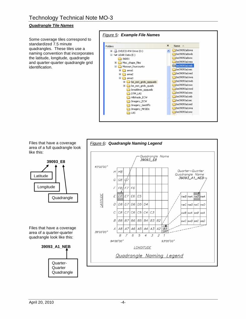
Figure 5: Example File Names
Figure 6: Quadrangle Naming Legend
Quadrangle Tile Names Some coverage tiles correspond to standardized 7.5 minute quadrangles. These tiles use a naming convention that incorporates the latitude, longitude, quadrangle and quarter-quarter quadrangle grid identification.
Files that have a coverage area of a full quadrangle look like this:
39093_E8
Files that have a coverage area of a quarter-quarter quadrangle look like this:
39093_A1_NEB
Latitude
Longitude
Quadrangle
Quarter-Quarter Quadrangle
Technology Technical Note MO-3
-5- April 20, 2010
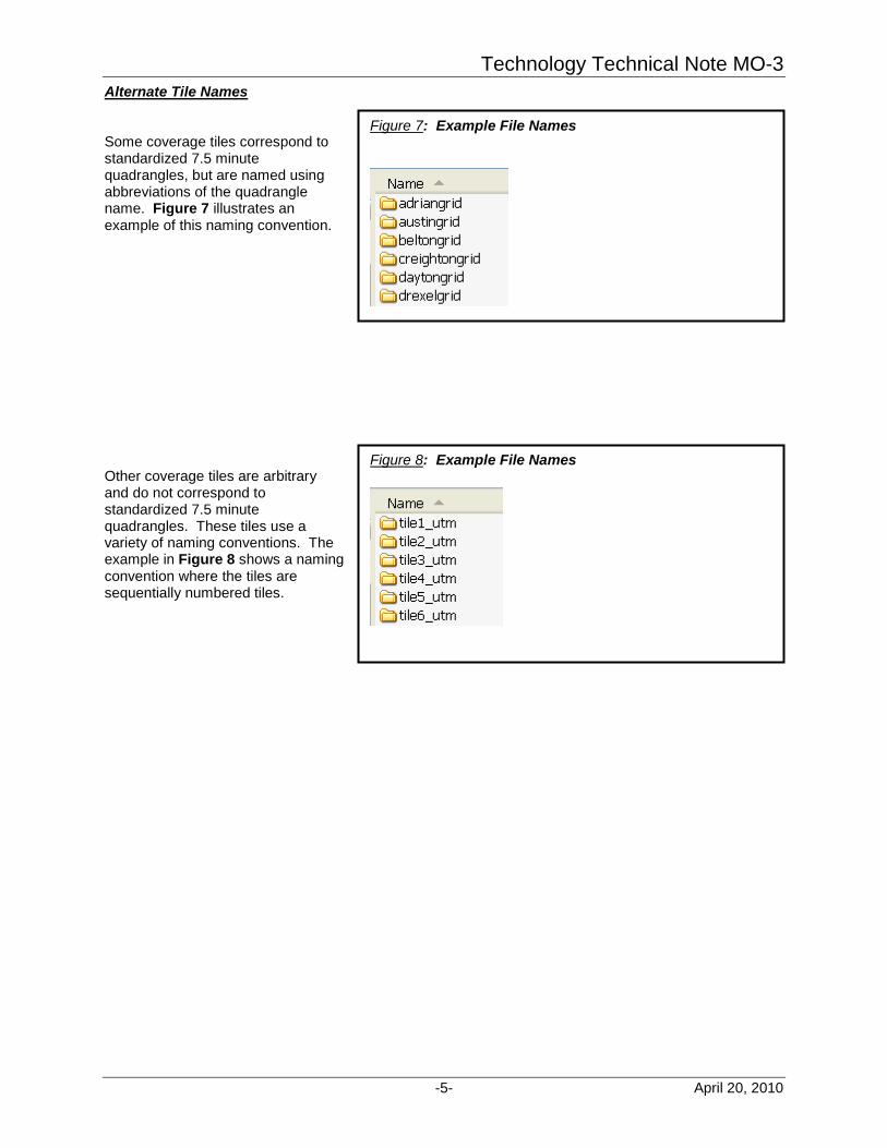
Figure 8: Example File Names
Figure 7: Example File Names
Alternate Tile Names Some coverage tiles correspond to standardized 7.5 minute quadrangles, but are named using abbreviations of the quadrangle name. Figure 7 illustrates an example of this naming convention.
Other coverage tiles are arbitrary and do not correspond to standardized 7.5 minute quadrangles. These tiles use a variety of naming conventions. The example in Figure 8 shows a naming convention where the tiles are sequentially numbered tiles.

Technology Technical Note MO-3
April 20, 2010 -6-
D.
Add ESRI Grid raster files using ArcMap’s Add Data button to add the desired ESRI Grid raster files to the project. The ESRI Grids are actually a series of files contained within a common folder. Do not navigate beyond the folder name when adding the ESRI Grids.
Adding and Displaying an ESRI Grid Raster
Using the Add Data dialogue box, set the Look in: box the correct folder. Next, select the desired ESRI Grid folder Then, click the Add button.

Technology Technical Note MO-3
-7- April 20, 2010
The ESRI Grid will be added and displayed with a grey scale color ramp that is keyed to elevations. The color ramp can be changed by double clicking on the color ramp legend associated with the ESRI Grid. This action will open a Select Color Ramp dialogue box from which a new color ramp can be picked.
With the color ramp in the example below, the highest elevations are displayed in green and the lowest are grey in color with red and yellow being in between.

Technology Technical Note MO-3
April 20, 2010 -8-
The raster display can be further customized by changing the Symbology to classify the color ramp according to a variety of methods. For example the color ramp can be set to correspond to an equally spaced elevation interval. The example below will classify the color ramp on even 1 meter intervals for areas with a ground surface between 225 and 245 meters: Begin by displaying the Layer Properties dialogue box for the ESRI Grid Raster and select the Symbology tab. Next click the Classify button to open the Classification dialogue box. Then click the Exclusion button. Set the Excluded values to 0-224; 246-1000 in order to exclude these values from the classification range. Click OK to close the dialogue box and return to the Classification dialogue box

Technology Technical Note MO-3
-9- April 20, 2010
Now select the Defined Interval method of classification and set the Interval Size to 1. This action will reset the Break Values to every meter in the elevation range of 225 to 245 Click OK to accept these changes in the classification of the color ramp. The map will now display the ESRI Grid with a color change every meter and the areas lower than elevation 225 or higher than 245 will not be displayed with any color as shown below:
Technology Technical Note MO-3
April 20, 2010 -10-
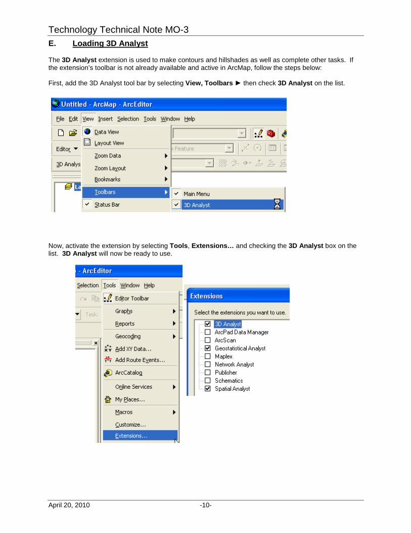
E.
The 3D Analyst extension is used to make contours and hillshades as well as complete other tasks. If the extension’s toolbar is not already available and active in ArcMap, follow the steps below:
Loading 3D Analyst
First, add the 3D Analyst tool bar by selecting View, Toolbars ► then check 3D Analyst on the list.
Now, activate the extension by selecting Tools, Extensions… and checking the 3D Analyst box on the list. 3D Analyst will now be ready to use.
Technology Technical Note MO-3
-11- April 20, 2010
F.
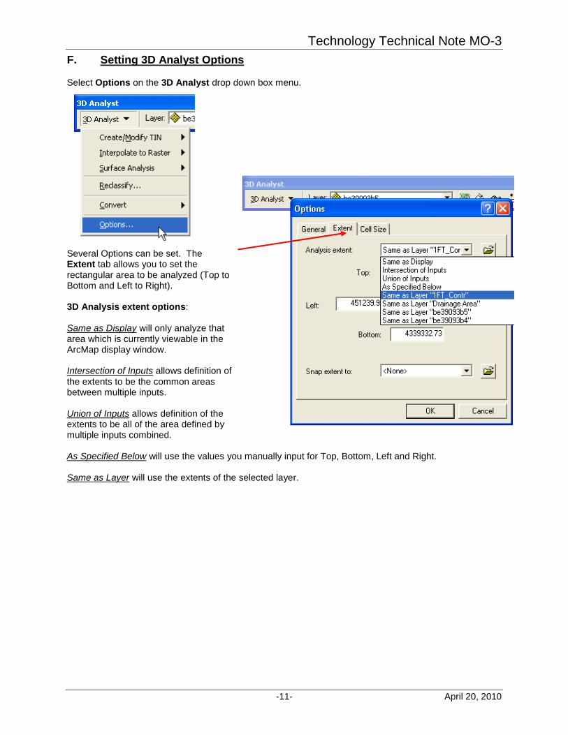
Select Options on the 3D Analyst drop down box menu.
Setting 3D Analyst Options
Several Options can be set. The Extent tab allows you to set the rectangular area to be analyzed (Top to Bottom and Left to Right). 3D Analysis extent options: Same as Display will only analyze that area which is currently viewable in the ArcMap display window. Intersection of Inputs allows definition of the extents to be the common areas between multiple inputs. Union of Inputs allows definition of the extents to be all of the area defined by multiple inputs combined. As Specified Below will use the values you manually input for Top, Bottom, Left and Right. Same as Layer will use the extents of the selected layer.

Technology Technical Note MO-3
April 20, 2010 -12-
The Cell Size tab allows the setting of the size of the raster cell that will be used to generate the surface analysis. The cell size will determine the density of the elevation points that represent the surface. A larger cell size will result in smoother contours; however, definition of surface features will be lost as the cell size increases. Cell Size Options: Maximum of Inputs will use the maximum cell size of the input layer. Minimum of Inputs will use the minimum cell size of the input layer. Note: Because all of the cells are the same size within a raster file, choosing either of the two options above will result in the same cell size if only one input layer is being used. As specified Below allows the manual input of the cell size. Same as Layer sets the cell size to match that of the selected layer.

Technology Technical Note MO-3
-13- April 20, 2010
G.
Contours can be generated from any of the ESRI Grid raster files using ArcMap’s 3D Analyst. Use the Add Data button to add the desired ESRI Grid raster file(s) to the project. See Section D. Adding and Displaying an ESRI Grid Raster.
Making Contours (Surface Analysis)
First, select Options on the 3D Analyst drop down box menu and set options as explained in Section E. Setting 3D Analyst Options.
After setting the Options, the contours are made using the tools available on the 3D Analyst tool bar. Use the pull down box to select the correct ESRI Grid raster folder (Target Layer) from which to make the contours.
Next, select Surface Analysis ► Contour on the 3D Analyst drop down box menu.

Technology Technical Note MO-3
April 20, 2010 -14-
Prepare to make the contours by setting the variables on the Contour dialogue box. Input surface: Using the pull down menu box set the Input surface to the correct ESRI Grid raster file. The surface elevations from this file will be used to generate the contours. Contour interval: This will determine the spacing interval between the contours. This will be in the same units as the elevations in the raster file if the Z factor is set to “1”. Base contour: The base contour is the first contour that is generated. The remaining contours will be spaced above and below the base contour at the contour interval. (For example using a base contour of “0.5” will generate contours at 700.5, 701.5, 702.5 and so on. Using a base contour of “0” will generate contours at 700, 701, 702, and so on.) Z Factor: The Z Factor is a number by which all of the raster cell elevation data will be multiplied. Using a Z factor of “3.28083333” will convert the contour lines from metric meters to U.S. Survey feet if the raster cell elevations are in meters, which is the case with this LiDAR data. Output features: The contours will be saved in an ESRI polyline shape file, the path and name of which is set at this menu location. In the example, the contours generated will be based upon elevations found in the be39093b5 raster file, the contour interval will be 1 foot and the contours will be to the even foot. The contours will be saved in an ESRI shape file named 1FT_Contr.shp in the C:\temp\ folder.

Technology Technical Note MO-3
-15- April 20, 2010
It is possible to generate a shape file containing a single contour. To make a shapefile with a single contour line set the Base contour value to the desired elevation for the contour line. Also set the Contour interval to a value that is larger than the difference between the Zmin and Zmax values so only the base contour will be generated. In this example a contour line at elevation 705 has been generated and saved in a shapefile named ctour705.
Technology Technical Note MO-3
April 20, 2010 -16-
H.
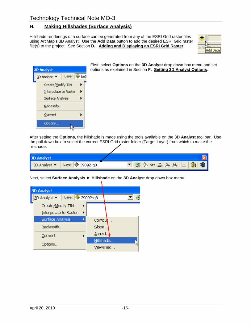
Hillshade renderings of a surface can be generated from any of the ESRI Grid raster files using ArcMap’s 3D Analyst. Use the Add Data button to add the desired ESRI Grid raster file(s) to the project. See Section D. Adding and Displaying an ESRI Grid Raster.
Making Hillshades (Surface Analysis)
First, select Options on the 3D Analyst drop down box menu and set options as explained in Section F. Setting 3D Analyst Options.
After setting the Options, the hillshade is made using the tools available on the 3D Analyst tool bar. Use the pull down box to select the correct ESRI Grid raster folder (Target Layer) from which to make the hillshade.
Next, select Surface Analysis ► Hillshade on the 3D Analyst drop down box menu.

Technology Technical Note MO-3
-17- April 20, 2010
Prepare to make the hillshade rendering by setting the variables on the Hillshade dialogue box. Input surface: Using the pull down menu box set the Input surface to the correct ESRI Grid raster file. The surface elevations from this file will be used to generate the hillshade. Azimuth: The angular direction of the illumination source. The default of 315 is usually O.K. to use. Altitude: The angle of the illumination source above the horizon. The default of 45 is usually O.K. to use. Leave Model shadows unchecked. Z factor: Leave the Z factor set to 1 unless the x,y units are different from the z units. The units for the NRCS supplied ESRI Grids should be the same. Output cell size: Defaults to the same cell size as the Input Surface. Output raster: The default is <Temporary>. Enter a path and file name if saving a permanent file is desired. In the example, the hillshade generated will be based upon elevations found in the be39092-g8 raster file, with an illumination source from the NW at 45 degrees above the horizon. The hillshade will be a temporary raster that will not be saved upon exit from ArcMap.

Technology Technical Note MO-3
April 20, 2010 -18-
The display properties of the Hillshade can be modified by right clicking on the Hillshade name, then selecting the Properties item from the pop up menu.
Select the Symbology tab and change the Stretch Type: to Standard Deviations with n: of 2. This setting generally results in a Hillshape image that provides good elevation relief.

Technology Technical Note MO-3
-19- April 20, 2010
I.
A land slope raster can be generated from any of the ESRI Grid raster files using ArcMap’s 3D Analyst. Use the Add Data button to add the desired ESRI Grid raster file(s) to the project. See Section D. Adding and Displaying an ESRI Grid Raster.
Making Slope Rasters (Surface Analysis)
The follow procedure is written assuming that the ESRI Grid raster files have a common unit of measure for x, y and z (i.e. all meters or all feet).
First, select Options on the 3D Analyst drop down box menu and set options as explained in Section F. Setting 3D Analyst Options.
After setting the Options, the slope raster is made using the tools available on the 3D Analyst tool bar. Use the pull down box to select the correct ESRI Grid raster folder (Target Layer) from which to make the slope raster.
Next, select Surface Analysis ► Slope on the 3D Analyst drop down box menu.
Technology Technical Note MO-3
April 20, 2010 -20-
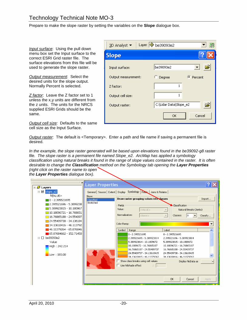
Prepare to make the slope raster by setting the variables on the Slope dialogue box. Input surface: Using the pull down menu box set the Input surface to the correct ESRI Grid raster file. The surface elevations from this file will be used to generate the slope raster. Output measurement: Select the desired units for the slope output. Normally Percent is selected. Z factor: Leave the Z factor set to 1 unless the x,y units are different from the z units. The units for the NRCS supplied ESRI Grids should be the same. Output cell size: Defaults to the same cell size as the Input Surface. Output raster: The default is <Temporary>. Enter a path and file name if saving a permanent file is desired. In the example, the slope raster generated will be based upon elevations found in the be39092-g8 raster file. The slope raster is a permanent file named Slope_e2. ArcMap has applied a symbology classification using natural breaks it found in the range of slope values contained in the raster. It is often desirable to change the Classification method on the Symbology tab opening the Layer Properties (right click on the raster name to open the Layer Properties dialogue box).

Technology Technical Note MO-3
-21- April 20, 2010
For example, change the number of classes to 6, set the Method to Manual and then edit the Break Values by entering 2, 5, 9, 14 and 20. then click OK The resulting classification for the example will appear a shown below:

Technology Technical Note MO-3
April 20, 2010 -22-
J.
Several statistics can be computed from a slope raster including calculating the mean of the slope values within an area such as a drainage area as in the following example:
Calculating the Mean Slope of an Area
Once the area has been defined with a shapefile use the Zonal Statistics tool that is one of the Spatial Analyst Tools within ArcToolbox
Technology Technical Note MO-3
-23- April 20, 2010
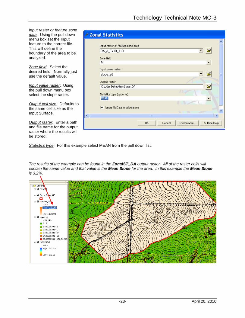
Input raster or feature zone data: Using the pull down menu box set the Input feature to the correct file. This will define the boundary of the area to be analyzed. Zone field: Select the desired field. Normally just use the default value. Input value raster: Using the pull down menu box select the slope raster. Output cell size: Defaults to the same cell size as the Input Surface. Output raster: Enter a path and file name for the output raster where the results will be stored. Statistics type: For this example select MEAN from the pull down list. The results of the example can be found in the ZonalST_DA output raster. All of the raster cells will contain the same value and that value is the Mean Slope for the area. In this example the Mean Slope is 3.2%.

Technology Technical Note MO-3
April 20, 2010 -24-
K.
A profile can be extracted from an ESRI Grid file using the profile tools in 3D Analyst.
Extracting a Profile
To extract a profile first select the Layer (ESRI_Grid) from which the profile will be drawn. Next, draw an alignment by selecting the Interpolate Line button from the 3D Analyst tool bar. Once the Interpolate Line tool is activated use the mouse pointer and a left click to establish points on the profile alignment. Double click to end the profile alignment.
Now that the profile alignment has been drawn, the profile graph can be created by selecting the Create Profile Graph button from the 3D Analyst tool bar.
The profile graph elevations will be in the same units as the ESRI Grid file. The distances will be in the units of the coordinate system currently set for the Data Frame properties. In this example the units are both meters. The graph will be plotted in the same order that the line was drawn (Distance zero, 0, will be the first point drawn.).

Technology Technical Note MO-3
-25- April 20, 2010
Right clicking while hovering the mouse pointer over the graph activates a pop-up menu that allows for customizing of the graphs appearance as well as exporting and printing of the profile. L.
In the example below, two ESRI_Grid rasters have been added to an ArcMap project. Both rasters are using the same color ramp to display the elevation range; however, a seam is created at the boundary of the two rasters. If the two rasters were merged into one then this boundary would be eliminated.
Merging ESRI Grid Files (Raster Mosaic)

Technology Technical Note MO-3
April 20, 2010 -26-
When a project area spans more than the coverage of a single ESRI Grid File it is helpful to merge the individual grid files into a single file. ESRI Grid Files can be merged using the Mosaic to New Raster tool that is one of the Data Management Tools within ArcToolbox Select the ESRI_Grid raster files that you want to mosaic. If the rasters have already been added to the ArcMap project then use the drop down list to select them. If the rasters have not been added to the project then use the browse
button to locate and select the raster files. Select an output location folder where the new raster will be stored. Type in a name for the new raster. Select 32_BIT_FLOAT for the Pixel type Click OK to make the new raster.
Technology Technical Note MO-3
-27- April 20, 2010
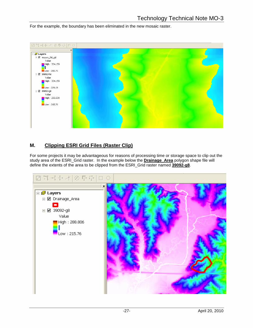
For the example, the boundary has been eliminated in the new mosaic raster.
M.
For some projects it may be advantageous for reasons of processing time or storage space to clip out the study area of the ESRI_Grid raster. In the example below the Drainage_Area polygon shape file will define the extents of the area to be clipped from the ESRI_Grid raster named 39092-g8.
Clipping ESRI Grid Files (Raster Clip)

Technology Technical Note MO-3
April 20, 2010 -28-
A portion of an ESRI Grid File can be clipped into a new ESRI_Grid raster file using the Clip tool that is one of the Data Management Tools within ArcToolbox Select the ESRI_Grid raster file that will be clipped. The rectangular extents of the clip can be set by either selecting an existing shape file from which the extent coordinates will be taken or the coordinates can be entered manually. Enter a path and file name for the new clipped raster. Click OK to make the new raster.

Technology Technical Note MO-3
-29- April 20, 2010
For the example, the extents of the new ESRI_Grid raster named Clip_39032-g8 match those of the Drainage_Area shape file.
N.
An alternative to clipping an ESRI Grid raster using Raster Clip is to use Extract by Mask. Using Extract by mask will clip the raster to a polygon instead of the polygon’s extents.
Clipping ESRI Grid Files (Extract by Mask)
Use the Extract by Mask, which is one of the Spatial Analyst Tools within ArcToolbox

Technology Technical Note MO-3
April 20, 2010 -30-
Input raster: Using the pull down menu box set the Input feature to the correct ESRI_Grid raster file. Input raster or feature mask data: Using the pull down menu box select the shapefile that will be used as the boundary for the extraction. Output raster: Enter a path and file name for the output raster where the results will be stored. Click OK to make the new raster. For the example, the border of the new ESRI_Grid raster named Extract_e2 match those of the DA_a_FY10_410 polygon shape file.

Technology Technical Note MO-3
-31- April 20, 2010
O.
The projection and units of the original LiDAR ESRI_Grid Raster files are not to be changed; however, it may be useful to change how ArcMap displays the x,y projection and units of those files.
Converting an ESRI Grid Raster from Meters to Feet
To change the x,y projection of ArcMap’s display select View, Toolbars ► then click Data Frame Properties. (This action does not actually change the projection of the ESRI_Grid raster file, but only how it is displayed in the current ArcMap secession.)
Under the Coordinate System tab, select a coordinate system that is in US Feet. If not already available then rename and modify an existing system as shown on the next page.
Technology Technical Note MO-3
April 20, 2010 -32-
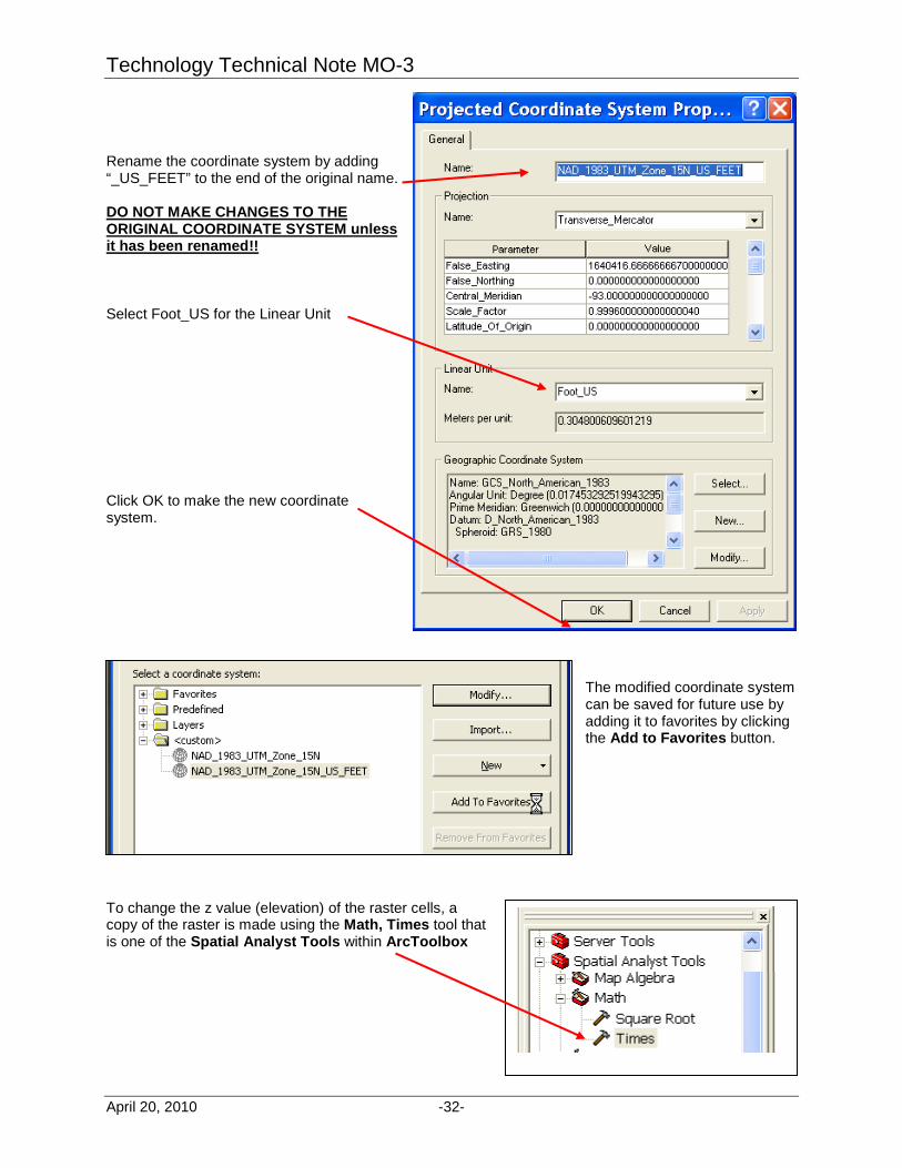
Rename the coordinate system by adding “_US_FEET” to the end of the original name. DO NOT MAKE CHANGES TO THE ORIGINAL COORDINATE SYSTEM unless it has been renamed!! Select Foot_US for the Linear Unit Click OK to make the new coordinate system.
The modified coordinate system can be saved for future use by adding it to favorites by clicking the Add to Favorites button.
To change the z value (elevation) of the raster cells, a copy of the raster is made using the Math, Times tool that is one of the Spatial Analyst Tools within ArcToolbox

Technology Technical Note MO-3
-33- April 20, 2010
Using the Times dialogue box, select the ESRI_Grid raster that will be converted. Also set the conversion constant for converting from meters to feet (3.2808333333) Enter the path and file name for the new ESRI_Grid raster file, then click OK to make the new raster.
In this example, the new ESRI_Grid raster named clip_31_Feet is used to create a profile graphic, which is now in the units of feet instead of meters.

Technology Technical Note MO-3
April 20, 2010 -34-
P.
It is possible to extract and ASCII x,y,z point file from an ESRI_Grid raster using ArcMap. This process involves creating a 2D Point feature file, then converting it to a 3D Point feature file and finally exporting to the ASCII point file. Since a 1 meter cell size raster will generate over 4,000 points per acre, it is advisable to prepare a clipped raster or a clipped feature point file that only includes the study area.
Extracting an ASCII x,y,z File from an ESRI Grid Raster
Making a 2D Point Feature. Select 3D_Analyst, Convert ► Raster to Features from the ArcMap toolbar. The setting of 3D Analyst ►Option ► Extent will be used when this command is used. See section F. Setting 3D Analyst Options. Set the Output geometry type first. Otherwise the ESRI Grids will not appear in the Input raster dropdown list. Output geometry type: Using the dropdown list, select Point. Input raster: Using the dropdown list select the correct ESRI_Grid raster, it is currently added to the ArcMap project. Otherwise using the browse button to navigate to the raster’s location. Output features: Enter or browse to the desired path and file name for the new feature (2D point shapefile) that will be created. Click OK to make the new feature file.
The new feature file will be automatically added to the ArcMap project. In this example it is named 2d_pt_g8.

Technology Technical Note MO-3
-35- April 20, 2010
Converting a 2D Point Feature to a 3D Point Feature. Select 3D_Analyst, Convert ► Features to 3D from the ArcMap toolbar. Input features: Using the dropdown list, select the 2D point feature. Click the Raster or TIN surface as the Source of heights. Raster or TIN surface: Using the dropdown list select the correct ESRI_Grid raster from which to extract the elevation data. Output features: Enter or browse to the desired path and file name for the new feature (3D point shapefile) that will be created. Click OK to make the new feature file.
The new feature file will be automatically added to the ArcMap project. In this example it is named 3d_pt_g8.

Technology Technical Note MO-3
April 20, 2010 -36-
Extracting an ASCII x,y,z point file from the 3D Point Feature. Using ArcToolbox, select 3D_Analyst Tools, Conversion, From Feature Class ► Feature Class Z to ASCII. Input Feature Class: Use the dropdown list to select the correct 3D Point Feature. Output Location: Browse to the folder where the ASCII file will be stored. Output Text File: Enter the name and extension for the ASCII point file. Output File Format: Using the dropdown list select XYZ. Delimiter: Using the dropdown list select the desired data separation character. Decimal Notation: Using the dropdown list select either Automatic or Fixed. Click OK to make the ASCII point file. In this example a text file named g8_XYZ_Pts.txt was created. The units will be the same as those from the raster file, in the example this is meters.

Technology Technical Note MO-3
-37- April 20, 2010
XYZ File Conversion If necessary, use the XYZ File Conversion program to convert the units of the ASCII point file (for example from meters to US Feet). The XYZ File Conversion program can be found in the Support_Files folder on the LiDAR drive.

Technology Technical Note MO-3
April 20, 2010 -38-
Q.
Break lines are helpful when using points that are actual LiDAR returns, which are usually stored as LAS files. The break lines define features such as channel banks or channel centerlines. Break lines for some coverage areas have been stored as ESRI Poly Z shapefiles. When importing these files into AutoCAD it may be desirable to first adjust the Z values from meters to feet using ArcMap.
Converting Elevations of Break Line Poly Z Files from Meters to Feet
DO NOT ADJUST THE Z VALUES OF THE ORIGINAL BREAKLINE FILES!! FIRST, Make a copy of the break line shapefile or extract the needed polylines to a new shapefile. This can be accomplished by right clicking on the break line shapefile then click Data ► Export Data. Give the new shapefile a name that implies that the Z values are in feet.

Technology Technical Note MO-3
-39- April 20, 2010
Once the new shapefile is created, use Adjust 3D Z, which is one of the Data Management Tools within ArcToolbox Input Feature: Use the dropdown list to select the new shapefile. Reverse Sign of Z Values: Leave this field blank. Adjust Z Value: Leave this field blank (if used it will add a constant value to every Z). Convert From Units: Select Meters. Convert To Units: Select Feet. Click OK to make the adjustment to the shapefile.

Technology Technical Note MO-3
April 20, 2010 -40-
R.
Contour lines are features contained in polyline shapefiles. A portion of a contour line can be used to produce a polygon feature from which an area can be calculated. For example, a series of polygons created using selected contour lines could be used to develop an elevation-area table for a pond’s storage area.
Using Contour Lines to Make Polygons
First create contours from an ESRI Grid raster. See Section G. Surface Analysis - Making Contours Next create or load an existing polyline shape file and add a line to it that represents a cutting line, centerline of dam for this example.

Technology Technical Note MO-3
-41- April 20, 2010
Now using the select features button, , on the ArcMap toolbar; pick the contour line from which to make the polygon. After selecting the line, right click on the shapefile containing the line in the table of contents and click Data ► Export Data… from the popup menu.
Complete the information in the Export Data dialogue box: Export: Set this to Selected features using the dropdown list. Output shapefile or feature class: Enter or browse to the desired path and file name for the new feature (polyline shapefile) that will be created to store the selected contour in.

Technology Technical Note MO-3
April 20, 2010 -42-
Once the new shapefile is created, use Feature To Polygon, which is one of the Data Management Tools within ArcToolbox to make a new polygon shape file where the new polygon will be stored. Complete the Feature To Polygon dialogue box: Input Features Select the shapefiles from the dropdown list that contains the contour line and the dam centerline. In this example those are the Ctour_l_704 and CL_l_Dam files. Output shapefile or feature class: Enter or browse to the desired path and file name for the new feature (polygon shapefile) that will be created to store the new polygon in.

Technology Technical Note MO-3
-43- April 20, 2010
The result is a new polygon shape file (Pool_a_704) containing a polygon from which an area can be
calculated using the measure tool, . In the example the area of the 704 contour is 2 acres.
As an alternative to the Measure Tool, the Calculate Area/Acres tool can be used to add an attribute field to the shapefile table. Using this method, the area of the polygon is permanently stored as part of the shapefile’s database.

Technology Technical Note MO-3
April 20, 2010 -44-
S.
Transferring points, lines and polygons from a digital model, like ArcMap, to the ground at a project site requires establishing benchmark references at the site. The benchmarks must be a reference for both horizontal (x,y) and vertical (z) datums.
Establishing Horizontal and Vertical Datums at a Project Site.
The preferred method of establishing a benchmark reference at a project site is to use an existing control point that has accurate coordinates such as a National Geodetic Survey (NGS) station control point. This would be accomplished by using appropriate surveying methods to establish a new benchmark at the site using the NGS station as a reference. An alternant method is to establish the new benchmarks using survey grade GPS equipment and the NGS Online Positioning User Service (OPUS). If establishing the benchmark using the above method is not an option, then an alternative is to use a mapping grade GPS receiver with a horizontal accuracy of 1 meter or less and a level. This method is less accurate and can easily introduce a couple of tenths of vertical error. It may not be suitable for all conservation practice needs. Use the following steps to complete this method:
1. Identify two or more areas in the project location that are relatively flat (+/- 0.2 feet) with a minimum area of 20 feet by 20 feet. The surfaces of these areas must not have been altered since the time of the LiDAR data accusation.
2. From the LiDAR data, determine the ground elevation of the areas and the horizontal coordinates
of the center of each area.
3. Using a mapping grade GPS, navigate to the center of one of the areas.
4. Set up a level and record a back sight (BS) rod reading. Using the LiDAR elevation of the ground in the center of the area and the BS, compute a height of instrument (HI).
5. Navigate to the center of the second area. Using the established HI, record a fore sight (FS) and calculate the elevation of the ground at this location. Compare the calculated elevation to the LiDAR elevation. If the difference between the two elevations is acceptable, +/-0.2 feet for example, then proceed to the next step. If the difference is unacceptable, then survey additional areas for comparison.
6. Once you have determined confidence in the HI’s relative accuracy as compared to the LiDAR elevation, use it to establish temporary benchmark(s) (TBM) at the site using appropriate surveying procedures.