materials

Article

Techno-Economic Assessment of a Scaled-Up MeatWaste Biorefinery System: A Simulation Study

Oseweuba Valentine Okoro 1,* , Zhifa Sun 1,* and John Birch 2

1 Department of Physics, University of Otago, P.O. Box 56, Dunedin 9054, New Zealand2 Department of Food Science, University of Otago, P.O. Box 56, Dunedin 9054, New Zealand;

john.birch@otago.ac.nz* Correspondence: okoos343@student.otago.ac.nz or oseweubaokoro@gmail.com or

oseweuba.okoro@otago.ac.nz (O.V.O.); zhifa.sun@otago.ac.nz (Z.S.);Tel.: +64-3-479-4006 (O.V.O.); +64-3-479-7812 (Z.S.)

Received: 29 January 2019; Accepted: 24 March 2019; Published: 28 March 2019�����������������

Abstract: While exports from the meat industry in New Zealand constitute a valuable source offoreign exchange, the meat industry is also responsible for the generation of large masses of wastestreams. These meat processing waste streams are largely biologically unstable and are capable ofleading to unfavourable environmental outcomes if not properly managed. To enable the effectivemanagement of the meat processing waste streams, a value-recovery based strategy, for the completevalorisation of the meat processing waste biomass, is proposed. In the present study therefore, abiorefinery system that integrates the biomass conversion technologies of hydrolysis, esterification,anaerobic digestion and hydrothermal liquefaction has been modelled, simulated and optimizedfor enhanced environmental performance and economic performance. It was determined that aninitial positive correlation between the mass feed rate of the waste to the biorefinery system and itsenvironmental performance exists. However, beyond an optimal total mass feed rate of the wastestream there is a deterioration of the environmental performance of the biorefinery system. It was alsodetermined that economies of scale ensure that any improvement in the economic performance of thebiorefinery system with increasing total mass feed rate of the waste stream, is sustained. The presentstudy established that the optimized meat waste biorefinery system facilitated a reduction in theunit production costs of the value-added products of biodiesel, biochar and biocrude compared theliterature-obtained unit production costs of the respective aforementioned products when generatedfrom stand-alone systems. The unit production cost of biogas was however shown to be comparableto the literature-obtained unit production cost of biogas. Finally, the present study showed that theoptimized meat processing waste biorefinery could achieve enhanced economic performance whilesimultaneously maintaining favourable environmental sustainability.

Keywords: meat waste biorefinery; economic performance; environmental performance; simulationstudy; optimization

1. Introduction

Biorefineries are systems that integrate different conversion technologies to generate multipleuseful products while using biomass as a renewable feedstock resource [1,2]. Based on this definition,a biorefinery may be considered as being similar to a typical crude oil refinery that employs crude oilas the feedstock to produce multiple useful products [1]. The renewability of biomass as a resourceprovides an opportunity for the development of sustainable pathways for the production of biofuelsand biochemicals. In line with current interest in the employment of the biorefinery paradigm as aviable approach to counter challenges of resource depletion and global warming [1,2], the present

Materials 2019, 12, 1030; doi:10.3390/ma12071030 www.mdpi.com/journal/materials

Materials 2019, 12, 1030 2 of 27

study has explored the viability of utilizing meat processing waste as a sustainable biomass resourcefor a biorefinery system. In this research, the country of New Zealand is specified as the case studywith meat processing waste investigated as a biomass feedstock that is sufficient to demonstrate thesustainability of the proposed biorefinery system. Meat processing waste has been specified as a viablebiomass resource in New Zealand since according to [1,3,4]:

• Significant masses of meat processing wastes are generated annually from meat processing relatedactivities in New Zealand.

• Meat processing wastes constitute major management challenges due to their unfavorable impactson land, water and air when improperly managed (Richard Stapel, Waste solutions- New Zealand,personal communication, 2015).

• Major technologies such as composting and incineration, employed in waste management in NewZealand, are characterized by several limitations such as requirements for large land area andlarge mass of bulking material, difficulty in dewatering the waste and the generation odorous air,dust and other emissions.

• Most importantly, meat processing wastes may serve as biomass resources that are availablein the absence of associated costs of cultivation, harvesting or agricultural land that typicallycharacterizes plant-sourced biomass.

• There is therefore a clear opportunity to improve the economic performance of existing meatprocessing plants, via the recovery of valuable products from the meat processing waste whichmay generate additional revenue streams when sold.

In recognition of the aforementioned benefits of utilizing meat processing waste as a sustainablebiomass resource, previous studies have experimentally explored the untapped potential of utilizingmeat processing waste biomass as a viable biorefinery feedstock [3–8]. These previous studies initiallyappreciated that the utilization of meat processing wastes as biorefinery feedstocks may present somechallenges as a result of its typically high moisture content. This is because most biomass conversiontechnologies favour dry biomass as feedstock for bioenergy and biochemicals production. A review ofexisting biomass technologies was therefore undertaken in [1] to enable the proper screening of thepossible biomass technologies and identify those technologies that would be sufficient to facilitate thetransformation of high moisture meat processing waste feedstocks. Biomass conversion technologies ofhydrolysis-esterification, anaerobic digestion and hydrothermal liquefaction conversion technologieswere consequently selected as the preferred technologies [3–7]. In the studies undertaken in [1,3–5],the conversion of the lipids present in the meat processing waste of high moisture dissolved airflotation sludge to biodiesel was considered crucial to the functionality of the proposed biorefinerysince there was a risk of anaerobic digestion (AD) failure if the high lipid concentrations in the inletstream to the AD process was maintained. Crucially the need to eliminate the high energy requirementthat would characterize any preliminary drying or dewatering operation, prior to lipid extractionnecessitated the approach of producing FAs via the so called ‘in-situ hydrolysis’ pathway. As statedearlier above moisture-favouring biomass conversion technologies of namely AD and hydrothermalliquefaction were integrated in the proposed biorefinery since they guarantee biofuel and biochemicalproduction respectively in the absence of the need for preliminary dewatering operations. Furthermore,the integration of the hydrothermal liquefaction process as a ‘terminal’ biomass conversion technologyeliminates the need for the incorporation of further downstream sterilization steps due to the hightemperature and high pressure conditions typically imposed [1,6–8].

These previous studies were therefore able to demonstrate the possibility of generating usefulproducts of biodiesel, biocrude, biochar and biogas from meat processing waste, via the employmentof biomass conversion technologies of hydrolysis-esterification, AD and hydrothermal liquefactionconversion technologies respectively [3–7].

Although the aforementioned biomass conversion technologies were shown to be feasible whenassessed via laboratory scale experiments, the viability and performance of the large-scale integration of

Materials 2019, 12, 1030 3 of 27

these biomass conversion technologies is yet to be assessed. In this study therefore, the environmentalperformance and economic performance of a large-scale biorefinery system operating in steady state,albeit simplified, will be investigated. The novelty of the study is emphasized by the unconventionalityof both the feedstocks employed and the complexity of the processing scheme of the proposedbiorefinery. Given that the biorefinery system is composed of selected biomass conversion technologiesthat have been extensively investigated in previous studies [3–7], the experimental results generatedfrom these studies will serve as an invaluable input data resource for the simulation study.

2. Process Modelling and Simulation Methodology

2.1. Process Modelling Software

The biorefinery system has been modelled and simulated using the commercially available ASPEN(Advanced System for Process Engineering, version10) plus. ASPEN plus is employed in processdesign, modelling and simulation [9]. ASPEN plus facilitates the resolution of process flowsheets byinvoking sequential modular and equation oriented modelling strategies [10]. Sequential modularmodelling and equation oriented modelling strategies enable ASPEN plus to resolve a large number ofunit operation blocks sequentially and solve a large number of equations (e.g., energy balance andmass balance equations) simultaneously [10,11].

2.2. Process Description

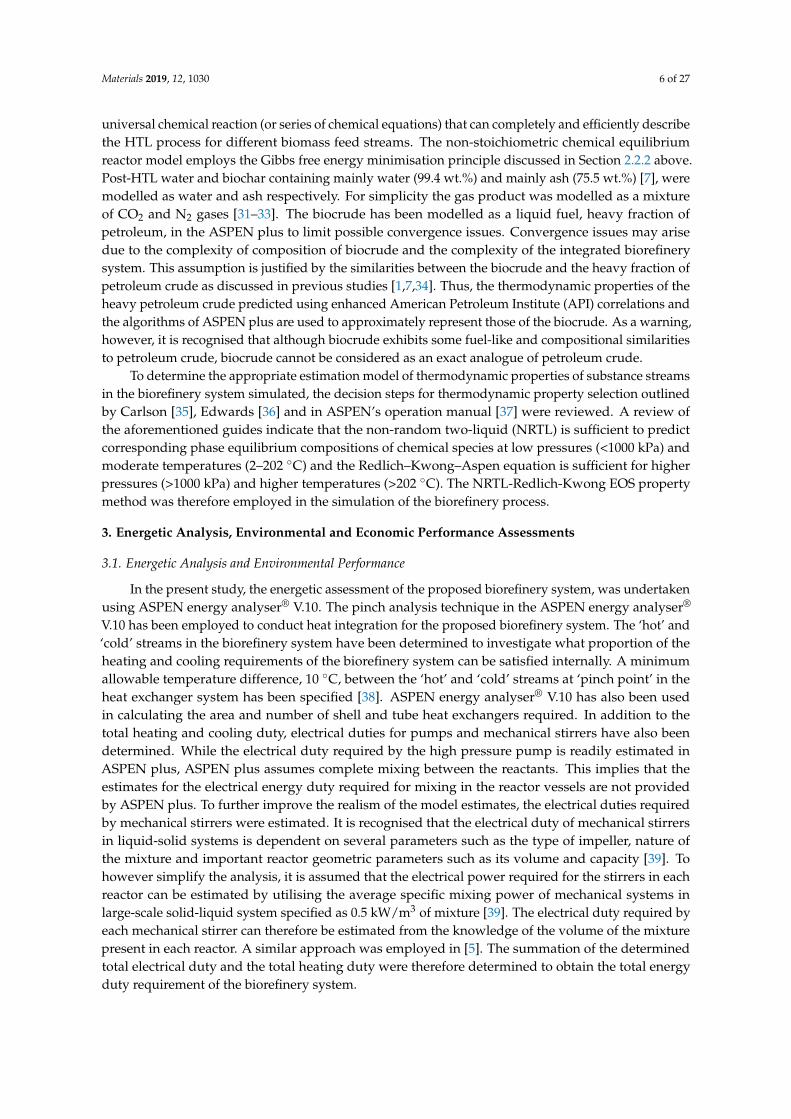
Figure 1 shows the schematic illustration of the biorefinery composed of the selected biomassconversion technologies. The system boundaries have been specified using the dashed lines in Figure 1.Figure 1 highlights the generation of the useful product streams, namely the biogas (gaseous biofuel),biodiesel (liquid biofuel), biochar (biomaterial for soil enhancement) and biocrude (biochemical sourceor liquid biofuel) from the meat processing waste streams of dissolved air flotation (DAF) sludgeand stockyard (SY) waste. It is assumed that the biorefinery system operates for 300 days/year(7200 h/year), all exit hot streams are cooled to 25 ◦C to enhance opportunities for heat recovery andthere is a base case availability of 1000 tonnes of DAF sludge per day (or 41.7 tonnes/h). The basecase mass feed rate of the SY waste will be determined from the mass feed rate of the DAF sludgeduring the simulation run. This is because the mass feed rate of the DAF sludge directly influences themass feed rate of wet hydrolysed DAF sludge (WHDS), from the in-situ hydrolysis processing of DAFsludge, employed for biomethane production as discussed in [6].

Materials 2019, 12, x FOR PEER REVIEW 3 of 28

operating in steady state, albeit simplified, will be investigated. The novelty of the study is emphasized by the unconventionality of both the feedstocks employed and the complexity of the processing scheme of the proposed biorefinery. Given that the biorefinery system is composed of selected biomass conversion technologies that have been extensively investigated in previous studies [3–7], the experimental results generated from these studies will serve as an invaluable input data resource for the simulation study.

2. Process Modelling and Simulation Methodology

2.1. Process Modelling Software

The biorefinery system has been modelled and simulated using the commercially available ASPEN (Advanced System for Process Engineering, version10) plus. ASPEN plus is employed in process design, modelling and simulation [9]. ASPEN plus facilitates the resolution of process flowsheets by invoking sequential modular and equation oriented modelling strategies [10]. Sequential modular modelling and equation oriented modelling strategies enable ASPEN plus to resolve a large number of unit operation blocks sequentially and solve a large number of equations (e.g., energy balance and mass balance equations) simultaneously [10,11].

2.2. Process Description

Figure 1 shows the schematic illustration of the biorefinery composed of the selected biomass conversion technologies. The system boundaries have been specified using the dashed lines in Figure1. Figure 1 highlights the generation of the useful product streams, namely the biogas (gaseous biofuel), biodiesel (liquid biofuel), biochar (biomaterial for soil enhancement) and biocrude (biochemical source or liquid biofuel) from the meat processing waste streams of dissolved air flotation (DAF) sludge and stockyard (SY) waste. It is assumed that the biorefinery system operates for 300 days/y (7200 h/y), all exit hot streams are cooled to 25 °C to enhance opportunities for heat recovery and there is a base case availability of 1000 tonnes of DAF sludge per day (or 41.7 tonnes/h). The base case mass feed rate of the SY waste will be determined from the mass feed rate of the DAF sludge during the simulation run. This is because the mass feed rate of the DAF sludge directly influences the mass feed rate of wet hydrolysed DAF sludge (WHDS), from the in-situ hydrolysis processing of DAF sludge, employed for biomethane production as discussed in [6].

Figure 1. Biorefinery system using meat processing waste as the feedstock. DAF denotes dissolved air flotation sludge, HTL denotes hydrothermal liquefaction.

Figure 1. Biorefinery system using meat processing waste as the feedstock. DAF denotes dissolved airflotation sludge, HTL denotes hydrothermal liquefaction.

Materials 2019, 12, 1030 4 of 27

2.2.1. Catalysed In-Situ Hydrolysis and Esterification of DAF Sludge

As shown in Figure 1, biodiesel is generated using the catalysed in-situ hydrolysis andesterification pathway. The generation of biodiesel from DAF sludge via the in-situ hydrolysis pathwayhas been simulated and discussed extensively in [5].

Briefly, in-situ lipid hydrolysis processing of the wet DAF sludge (92 wt.% wet basis) is achievedunder the imposed reaction conditions of temperature, pressure and catalyst load of 92.5 ◦C, 1 atmand 0.09216 kg-Dowex 50 WX2 resin/kg-wet fresh DAF sludge respectively according to a previousstudy [3]. DAF sludge lipids (DSL) have been modelled using Zong’s Fragment-based approach asextensively discussed elsewhere [12]. The protein content and carbohydrate content of DAF sludgeare modelled as L-phenylalanine [13] and glucose [14] respectively. Other chemical inputs such asmethanol, water and glycerol employed in the simulation study were obtained from the databank ofthe chemical property library in ASPEN plus® V10. It has been proposed that DSL hydrolysis reactionoccurs as follows,

DSL + 3H2Ocatalyst→ Glycerol + 3DFA (1)

where DFA represents DAF sludge fatty acids.This DSL hydrolysis reaction has been simulated using a simple stoichiometric reactor block in

ASPEN plus, with a 98% conversion of the DSL imposed [15]. This preliminary simulation studyassumes complete recoverability of the Dowex 50 WX2 resin beads for simplicity. For the esterificationreaction, the DAF sludge fatty acid, DFA, is modelled as oleic acid due to reasons discussed inReference [5], with methylation achieved using excess methanol [5,16]. The esterification reaction ishomogeneous first-order reaction occurring under the action of 0.0354 kg of solid 12-tungstophosphoricacid (as the catalyst) per kg of DAF fatty acid and supported on silica [16]. The esterification reactionis modelled according to the following reaction equation,

DFA + Methanolcatalyst→ DSME + water (2)

where, DSME denotes the DAF sludge methyl ester.

2.2.2. Anaerobic Co-Digestion Process of WHDS and SY

The wet hydrolysed dissolved air flotation sludge (WHDS) residue is subjected to an anaerobicdigestion process while utilizing the stockyard (SY) waste stream as a co-digestion substrate to enhancethe useful biomethane potential via the introduction of established synergizing effects [6]. According toOkoro et al. [6] the preferred mix ratio of the mass of stockyard waste to the mass of WHDS is 4 to 1, ona volatile solid basis for a favourable biomethane yield from an anaerobic digestion process occurringat a temperature condition and pressure condition of 37 ◦C and 1 atm respectively. To model theanaerobic digestion process, it is recognized that the AD process is an exceptionally complex biologicalprocess defined by a series of multi-step, overlapping processes that are dependent on numerousfactors such as the microbial population growth and decline, nutrient content, pH value, temperatureand inoculum substrate ratio [1,6]. Several simplifying specifications were therefore imposed to enablethe successful simulation of the anaerobic digestion process. Firstly, it was assumed that equilibriumstates exist during the degradation process, with the biogas potential for the specified substrate mixcalculated by minimizing the Gibbs free energy (G) of the system while simultaneously satisfying massbalance and energy balance constraints. This assumption is justified since the degradation reactionsthat occur during the anaerobic digestion process always attain rates such that the reacting species areclose to their respective equilibrium states (∆Gtotal = 0) [17]. The total Gibbs free energy Gtotal for theAD system with N species is expressed by the following equation [18,19],

Gtotal =N

∑i=1

niG0f .i +

N

∑i=1

(niRT ln

(fifi

o

))(3)

Materials 2019, 12, 1030 5 of 27

where for gas phase species, fi0 is equal to 1 bar and,

fi = θiyiP (4)

and for liquid phase species,fifi

o = ai (5)

In the above equations, fi0 denotes the standard molar fugacity of species i, Gf,i0 is the Gibbs free

energy of formation of species i at standard pressure of 1 bar; θi is the fugacity coefficient of species i;R is the universal gas constant specified as 8.314 J/mol·K, T is the temperature in K, ai is the activityof species i, yi is the mole fraction vapour of specie i. ASPEN plus is able to minimise the objectivefunction (Gtotal) by setting the differentiated equation (with respect to ni) and subsequently solving forni. Fugacities, activities and fugacity coefficients are estimated by ASPEN plus using thermodynamicproperty methods. A similar approach is taken when assessing both complex chemical equilibria andcomplex phase equilibria for all chemical species. Secondly, the experimentally determined biomethanepotential expressed as the volume of biomethane produced in mL per unit mass of volatile solidsin g in [6] has been employed as the biomethane potential of the anaerobic process in the presentsimulation study. This constitutes a common methodology that has been extensively applied to processsimulations of AD processes [20–24]. Thirdly to specify the fraction of the available organic substratesthat can be degraded anaerobically for biomethane production, the anaerobic biodegradability ofthe substrate mixture is another important parameter important for a successful simulation of theanaerobic co-digestion process. The anaerobic biodegradability (Xd) of a substrate mixture is calculatedby comparing the experimentally determined biomethane potential (BMPe) in mL/g-VSadded fromthe co-substrate mixture with the associated theoretical maximum biomethane potential (BMPt) inmL/g-VSadded determined using Equation (6) below,

Xd =BMPe

BMPt(6)

This anaerobic biodegradability (Xd) is numerically equivalent to the mass fraction of thesubstrate volatiles available that can be degraded under the anaerobic conditions. The experimentallydetermined biomethane potential (BMPe) can be obtained from the results presented in Reference [6]while the theoretical maximum biomethane potential (BMPt) is calculated using Buswell’s relation,which is based on the elemental content of the substrates, as follows [25–28],

BMPt =

22400[( c

2

)+

(h8

)−( o

4

)−(

3n8

)−( s

4

)](12c + h + 16o + 14n + 32s)

(7)

where c, h, o, n and s are subscripts representing the number of atoms present in organics with achemical formula of CcHhOoNnSs which represents the substrate mixture being degraded anaerobically.The chemical formulae of stockyard waste and wet hydrolysed DAF sludge residue were estimated tobe C297H504N18O169S and C48H79N2O17S respectively [6].

2.2.3. Hydrothermal Liquefaction Process of Digestate

In previous studies, the hydrothermal liquefaction process was shown to be characterised bythe presence of equilibrium states [29,30]. Variations of the reaction equilibrium conditions weredemonstrated as having implications on the biochar yield and biocrude yield [29,30]. Recognisingthe complexity of the hydrothermal liquefaction process, the yields of the major products namelybiocrude, biochar, gas phase and post-HTL water were also predicted using the non-stoichiometricchemical equilibrium reactor model of the ASPEN plus. The non-stoichiometric chemical equilibriumreactor model was employed since there is currently no consensus among researchers with respect to a

Materials 2019, 12, 1030 6 of 27

universal chemical reaction (or series of chemical equations) that can completely and efficiently describethe HTL process for different biomass feed streams. The non-stoichiometric chemical equilibriumreactor model employs the Gibbs free energy minimisation principle discussed in Section 2.2.2 above.Post-HTL water and biochar containing mainly water (99.4 wt.%) and mainly ash (75.5 wt.%) [7], weremodelled as water and ash respectively. For simplicity the gas product was modelled as a mixtureof CO2 and N2 gases [31–33]. The biocrude has been modelled as a liquid fuel, heavy fraction ofpetroleum, in the ASPEN plus to limit possible convergence issues. Convergence issues may arisedue to the complexity of composition of biocrude and the complexity of the integrated biorefinerysystem. This assumption is justified by the similarities between the biocrude and the heavy fraction ofpetroleum crude as discussed in previous studies [1,7,34]. Thus, the thermodynamic properties of theheavy petroleum crude predicted using enhanced American Petroleum Institute (API) correlations andthe algorithms of ASPEN plus are used to approximately represent those of the biocrude. As a warning,however, it is recognised that although biocrude exhibits some fuel-like and compositional similaritiesto petroleum crude, biocrude cannot be considered as an exact analogue of petroleum crude.

To determine the appropriate estimation model of thermodynamic properties of substance streamsin the biorefinery system simulated, the decision steps for thermodynamic property selection outlinedby Carlson [35], Edwards [36] and in ASPEN’s operation manual [37] were reviewed. A review ofthe aforementioned guides indicate that the non-random two-liquid (NRTL) is sufficient to predictcorresponding phase equilibrium compositions of chemical species at low pressures (<1000 kPa) andmoderate temperatures (2–202 ◦C) and the Redlich–Kwong–Aspen equation is sufficient for higherpressures (>1000 kPa) and higher temperatures (>202 ◦C). The NRTL-Redlich-Kwong EOS propertymethod was therefore employed in the simulation of the biorefinery process.

3. Energetic Analysis, Environmental and Economic Performance Assessments

3.1. Energetic Analysis and Environmental Performance

In the present study, the energetic assessment of the proposed biorefinery system, was undertakenusing ASPEN energy analyser® V.10. The pinch analysis technique in the ASPEN energy analyser®

V.10 has been employed to conduct heat integration for the proposed biorefinery system. The ‘hot’ and‘cold’ streams in the biorefinery system have been determined to investigate what proportion of theheating and cooling requirements of the biorefinery system can be satisfied internally. A minimumallowable temperature difference, 10 ◦C, between the ‘hot’ and ‘cold’ streams at ‘pinch point’ in theheat exchanger system has been specified [38]. ASPEN energy analyser® V.10 has also been usedin calculating the area and number of shell and tube heat exchangers required. In addition to thetotal heating and cooling duty, electrical duties for pumps and mechanical stirrers have also beendetermined. While the electrical duty required by the high pressure pump is readily estimated inASPEN plus, ASPEN plus assumes complete mixing between the reactants. This implies that theestimates for the electrical energy duty required for mixing in the reactor vessels are not providedby ASPEN plus. To further improve the realism of the model estimates, the electrical duties requiredby mechanical stirrers were estimated. It is recognised that the electrical duty of mechanical stirrersin liquid-solid systems is dependent on several parameters such as the type of impeller, nature ofthe mixture and important reactor geometric parameters such as its volume and capacity [39]. Tohowever simplify the analysis, it is assumed that the electrical power required for the stirrers in eachreactor can be estimated by utilising the average specific mixing power of mechanical systems inlarge-scale solid-liquid system specified as 0.5 kW/m3 of mixture [39]. The electrical duty required byeach mechanical stirrer can therefore be estimated from the knowledge of the volume of the mixturepresent in each reactor. A similar approach was employed in [5]. The summation of the determinedtotal electrical duty and the total heating duty were therefore determined to obtain the total energyduty requirement of the biorefinery system.

Materials 2019, 12, 1030 7 of 27

The energy potential of the proposed biorefinery system is estimated from the knowledge of theyield and higher heating values (HHVs) of the energy dense product streams. In this study the NER isutilised as a simple environmental performance index, since its sufficiency as a surrogate measure ofenvironmental sustainability was previously demonstrated [40,41]. The NER of the biorefinery systemis defined as follows,

NER =

n∑j

(HHVj × Pj

)

S∑i

Es−E,i + Ep−E

ηH−E

+

N∑i

EH− f ,i

ηC−H

(8)

where HHVj represents the higher heating value of the jth energy dense product (the HHV of biodiesel,biogas and biocrude have been determined to be 39,800 [4], 20,900 [6] and 36,700 kJ/kg [7,34]respectively; Pj represents the production capacity of the jth energy dense products of biodiesel,biocrude and biogas, in kg/h, the other useful product of biochar is not considered as an energy densefuel due to its low HHV of 4580 kJ/kg as discussed in Reference [6]; EH−f,i denotes the input thermalenergy in kJ/h for the ith major equipment; Es−E,i represents the electrical energy required by the ithstirrer; Ep−E represents the electrical energy required by the HTL high pressure pump; ηC−H and ηH−Erepresent the thermal efficiencies of conversion of chemical energy (biodiesel, biocrude and biogas)to thermal energy and electrical energy, respectively, which are specified as 0.9 and 0.47 [42–44]; n, Sand N are the number of energy dense products, number of reactor stirrers and number of equipment.For countries such as New Zealand where electricity can be generated from renewable sources suchas hydropower, the electrical energy term will be ignored. This is because renewable energy sourcesare not associated with unfavorable environmental impacts and unpleasant sustainability concerns.Two cases, electricity generation from fossil sources (case A) and electricity generation from renewablesources (case B) will therefore be assessed in this study. For both cases A and B, an NER value greaterthan 1 is indicative of a favorable environmental performance [45].

3.2. Economic Assessment of the Biorefinery System

To investigate the economic performance of the biorefinery system several economic assessmentmetrics have been initially considered. These economic assessment metrics are namely, the productioncost per unit higher heating values of the useful products, (Ch,j), in $US/MJ in year j, the productioncost per unit price of the useful products (Cp,j) (dimensionless) in year j and the production cost perunit mass of useful products (Cm,j) in $US/tonne, in year j. These economic assessment metrics arecalculated using the following equations, respectively,

Ch,j =CT,j

n∑

i=1mp,iHHVi

(9)

Cp,j =CT,j

n∑

i=1mp,i pi

(10)

Cm,j =CT,j

n∑

i=1mp,i

(11)

where in Equations (9)–(11), CT,j is the total annual cost of the biorefinery system in $US in year j; mp,iis the mass of the ith useful product of biochar, biodiesel, biocrude and biogas generated per year intonne/yearear; HHVi is the higher heating value of the ith useful product in MJ/tonne; pi is the unitmarket price of the ith useful product in $US.

Materials 2019, 12, 1030 8 of 27

The economic assessment metric of Equation (9) is based on the energy content of the usefulstreams thus emphasising the product streams of biocrude, biodiesel and biogas that are typicallyenergy dense. This economic assessment metric therefore erroneously considers the biochar productstream as less valuable since it presents a low HHV of 4.58 MJ/tonne [7,34]. Thus, since Equation (9)does not consider the value of biochar as a viable soil additive, it may present a distorted view of theperformance of the biorefinery system. The economic assessment metric of Equation (10) emphasesthe market prices of biocrude, biodiesel, biogas and biochar. Unfortunately, at the time of preparingthis manuscript, there is no data available in the literature highlighting the market price of biocrudeand biochar products, thus limiting the applicability of Equation (10). The economic assessment metricof Equation (11) considers all product streams as equally valuable, since the equation defines theproduction cost per unit mass of useful products, Cm, with the mass, mp,i, of each useful product iemployed as a unifying quantitative input in economic performance estimation.

Therefore, due to the limitations of Equations (9) and (10) discussed above, the present studywill employ production cost per unit mass of the useful products as a sufficient economic assessmentmetric for economic performance assessment. This is because the production cost per unit mass ofuseful products, Cm, does not consider any of the products (such as biochar) less valuable than others(biodiesel, biocrude and biogas) as in Equation (9) and also does not require the knowledge of themarket prices of the products, as in Equation (10). Since Equation (11) employs the mass of eachproduct stream as the unifying property of the biorefinery system in the absence of the highlightedlimitations other economic performance assessment metrics discussed above, the production cost perunit mass of useful product will constitute a satisfactory indicator of the economic performance of themeat processing waste biorefinery system. The equations employed in unit product cost estimationpreviously reported in Reference [5] have therefore been employed.

In Equation (11), therefore, CT is calculated as follows [46],

CT,j = CAECC,j + CAOC,j (12)

where CAECC,j represents the annual equivalent capital cost in $US in year j and CAOC,j represents theannual operating cost in $US in year j.

In Equation (12), the annual equivalent capital cost in year j, CAECC,j, can be estimated using thefollowing equation [46],

CAECC,j = It,j ×[(1 + i)n × i(1 + i)n − 1

](13)

where, i represents the interest rate, specified as 10%, n represents the plant lifespan, assumed to be 10years and It,j represents the total investment cost in $US in year j, which is estimated as follows,

It,j = IM,j + IHEN,j (14)

In this Equation (14), IM,j represents the investment cost of major equipment in $US in year j andIHEN,j represents the investment cost of the heat exchanger network (after heat integration) in $US inyear j. The investment cost of major equipment IM can be evaluated by the following equations [46,47],

IM,j = 1.81× EISBL,j (15)

EISBL,j = fL

n

∑i

Costi,j (16)

where, EISBL represents the inside battery limit equipment cost in $US per year j, fL represents the Langfactor, given as 3.60 for mixed fluid-solid processing plants [45,46] and Costi represents the equipmentpurchase cost for the ith equipment in $US in year j.

Materials 2019, 12, 1030 9 of 27

To calculate the investment cost of the heat exchanger network (after heat integration), the defaultcosting methodology in ASPEN energy analyser® V.10 is used to estimate the investment cost of theheat exchanger network (HEN) in $US for year 2016, as follows,

IHEN,2016 = 10,000 + 800N(

AN

)0.8(17)

where A represents the area of the heat exchanger network in m2 and N represents the number ofshell and tube heat exchangers; IHEN,2016 represents the cost of the HEN in year 2016 and is applied inEquation (14) above.

Equipment costing and sizing have been calculated using the ASPEN process economic analyser(APEA). Given that the APEA database are based on equipment cost data from 2016 (ASPEN technologyInc., personal communication, 1 August 2017) the chemical engineering plant cost index (CEPCI) isutilised in estimating the current capital plant cost for the year, 2018 (data for 2019 not available at thistime), as follows [48],

It,2018 = It,2016

(CEPCI2018

CEPCI2016

)(18)

In Equation (18), It,2016 is the total investment cost, calculated based on equipment purchasecosts in year 2016 (Equation (14)). The values for CEPCI2018 and CEPCI2016 were reported on thechemengonline website as 576.4 (as at 2018) and 541.7 respectively.

The purchase cost of the mechanical stirrers is not estimated by the ASPEN process economicanalyser since ASPEN plus assumes complete mixing as discussed above. Therefore, the purchase costof the mechanical stirrers is introduced to the equipment purchase cost. Assuming the mechanicalstirrers utilised in each reactor vessel is a propeller type, the purchase cost of the mechanical stirrers isestimated as follows [48,49],

Costs,2016 = 4866.924 + 2173.138S0.8 (19)

where Costs,2016 is the cost of the stirrer in $US, in 2016 and S is the electrical power requirement of thestirrer in kW. This calculated cost is employed in Equation (16).

The annual operating cost in year 2018, CAOC,2018, in Equation (12), refers to the cost associatedwith utilities such as energy, labour, repairs, maintenance and raw materials consumed by thebiorefinery per year can be estimated as follows [48,50],

CAOC,2018 = Lc + Cc + Dc + Rm + Ec + Vc (20)

where Lc represents the labour cost in $US, Cc represents the chemical cost in $US, Dc represents thedepreciation cost in $US, Rm represents the repair and maintenance cost in $US, Ec represents theenergy cost in $US and Vc represents the overhead cost in $US.

All operating costs have been therefore also been evaluated for the year, 2018. These parametersare estimated as follows [46–50],

Lc =[(

15× l f

)+ (3× ls)

](21)

Cc = tn

∑i

uc,i ×mc,i (22)

Dc =It,2018

n(23)

Rm = 0.06× It,2018 (24)

Ec = [(uh × h) + (ue × e)] (25)

Materials 2019, 12, 1030 10 of 27

Vc = 0.05(Dc + Lc + Ec) (26)

In Equations (21)–(26), lf represents the labour cost per year for each plant worker andspecified as $US 36,672/year [51], ls represents the labour cost per year for each supervisor specifiedas $US 56,000/year [52], the constant values 15 and 3 refer to the assumed number of plantworkers and supervisors required onsite; uc,i is the unit cost of the ith chemical in $US/kg (froma commercial website-alibaba.com, assessed on the 24th of February 2018),

.mc,i is the mass feed

rate of the ith chemical in kg/yearear; t is the time in years; uh is the unit heating cost specified as$US 2.48 × 10−6 per kJ [53], h is the total heat energy per year in kJ, uh is the unit electrical energy costspecified as $US 0.0681 kW−1 h−1 [54] and e is the total electrical energy per year in kW h.

As discussed in [5], it is assumed that fresh batches of the resin are introduced every three months.It is also assumed that fresh batches of the solid 12-tungstophosphoric acid catalyst, employed duringDFA esterification reactions, are required every three months. The solid 12-tungstophosphoric acidcatalyst has also assumed to be localised within the reactive distillation column to greatly simplify thesimulation study.

3.3. Mass Feed Rate of the Processing Waste Streams

Processing variables such as the conditions of temperature and pressure and physiochemicalproperties of the waste streams may influence the performance of the biorefinery system. However,a comprehensive consideration of the biorefinery design challenges suggests that the mass feed rateof the meat processing waste streams of stockyard (SY) waste and DAF sludge may constitute veryimportant parameters that may vary significantly and also influence the viability of the biorefinerysystem. This is because the mass feed rate of DAF sludge influences not only the biodiesel yield fromthe hydrolysis and esterification of the DSL and DFA respectively but also influences the mass feedrate of the WHDS residue. The mass feed rate of the WHDS residue in turn, influences the mass feedrate of SY waste, with the mass feed rate of the WHDS and SY waste mixture influencing the biogaspotential from the anaerobic co-digestion process. The mass feed rate of the digestate by-productfrom the anaerobic co-digestion influences the biocrude, biochar, gas and post-HTL water yield fromthe HTL process. Clearly the mass feed rates of the waste streams (SY waste and DAF sludge) willtherefore significantly influence the overall environmental performance and economic performance ofthe biorefinery system.

In this study therefore, the variation in the environmental performance, in terms of the NERvalue and the variation in the economic performance, in terms of unit production cost of the usefulproducts, Cm, is assessed. To simplify future reference to the total meat processing waste stream,the total meat processing waste stream of DAF sludge and SY waste will be represented using totalmeat processing waste stream (TMPS) as an abbreviation in subsequent texts. The dependence of theNER and the dependence of the unit production cost Cm on the mass feed rate TMPS, is assessed fordifferent mass feed rates, ranging from 50% to 150% of the base case. For clarity the base case is definedas the biorefinery system that can process the mass feed rates of the DAF sludge (41.7 tonnes/h), SYwaste (dependent on the mass feed rate of DAF sludge based on the discussions above) and TMPS(equal to sum of mass feed rate of DAF sludge and mass feed rate of SY waste). All the analysis stepsspecified in Section 3 above have been carried out for the different scenarios of the processing wastemass feed rates.

3.4. Optimization of Biorefinery System

It is important to determine the optimum mass feed rate of TMPS in order to obtain enhancedenvironmental performance and enhanced economic performance of the biorefinery system. Sincethe economic performance and the environmental performance may be in competition with eachother, biorefinery optimization is achieved when process conditions that enable the best compromisebetween the economic performance and the environmental performance are determined. To determine

Materials 2019, 12, 1030 11 of 27

the mass feed rate of TMPS for such a compromise, a multiple objective optimization of the objectivefunctions of environmental performance and the economic performance has been undertaken in thisstudy. Multi-objective optimization was achieved using the numerical optimization algorithm inthe JMP software (Version 14.0.0., SAS Inc., Cary, NC, USA). This optimization algorithm appliesthe extensively employed numerical desirability function in converting the objective functions ofeconomic and environmental performances into a single objective function for easy optimization asdiscussed in previous studies [55–57]. Extensive discussions relating to this optimization methodologyare also presented elsewhere in References [58–61]. Therefore, using the JMP software, the value of theindependent variable (mass feed rate of TMPS stream) that best provides a trade-off between competingresponses (environmental performance and economic performance) therefore has been determined.

4. Results and Discussions

4.1. Description of the Modelled Process

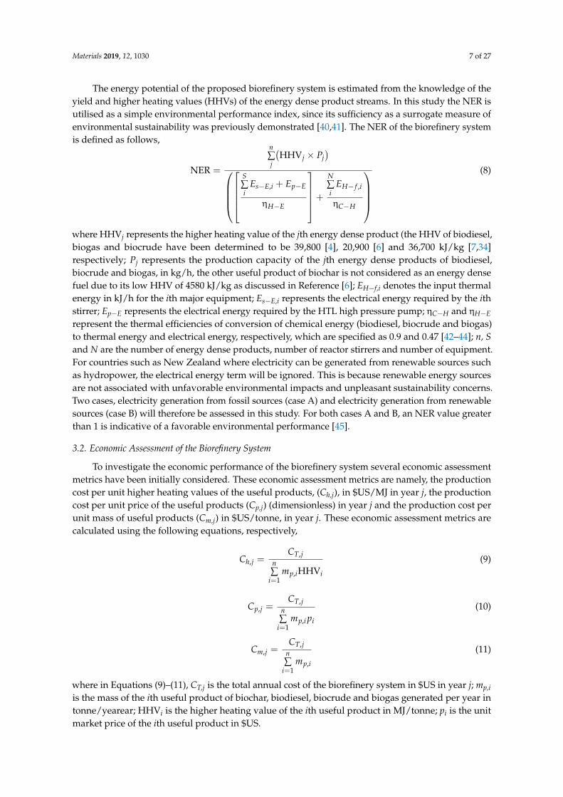
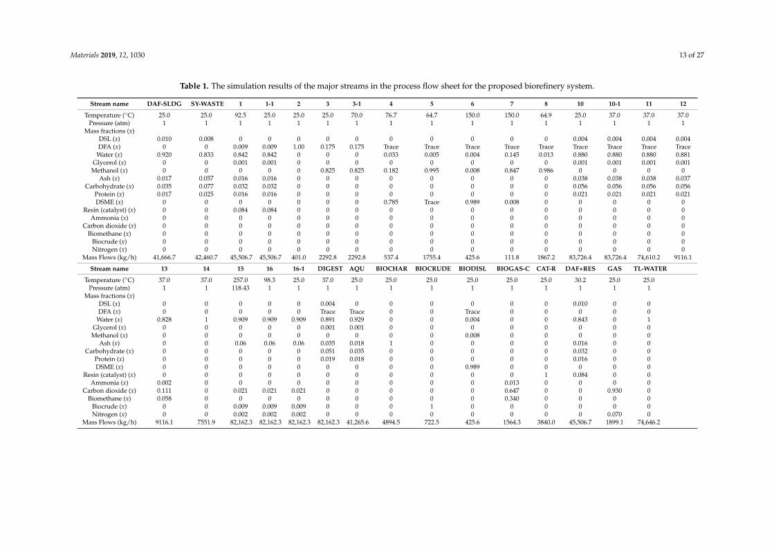
The modelled flow chart of the biorefinery system is presented in Figure 2. In this figure,dashed blocks 1, 2 and 3 represent the major biomass conversion processes of the biorefinerysystem: integrated in-situ hydrolysis and esterification process, anaerobic co-digestion processand hydrothermal liquefaction process responsible for the major products of biodiesel, biogas andbiocrude and biochar respectively. The detailed individual operation units and the mass streamsof the biorefinery system are also shown in Figure 2. The modelled results of the mass flow rates,temperatures, pressures, mass fractions of the streams are listed in Table 1 in that table together withthe assigned process input data of the mass flow rate, temperature, pressure of the feedstock streams.

4.1.1. The integrated In-Situ Hydrolysis and Esterification Process

As shown in the dashed block 1 in Figure 2 and discussed in Reference [5], the inlet feed stream,wet DAF sludge (stream DAF-SLDG) containing 92 wt.% moisture content (wet basis) at a mass flowrate of 1000 t/day (41667 kg/h), temperature of 25 ◦C and pressure of 1 atm and the resin-catalyststream (RESIN-CT) at a mass flow rate of 3840 kg/h, temperature of 25 ◦C and pressure of 1 atm, areinitially mixed (MIX-1) and the mixture is fed to the in-situ lipid hydrolysis reactor (H-REACT).

The in-situ hydrolysis reaction temperature is specified as 92.5 ◦C and the reaction pressurespecified as 1 atm as determined in [3]. Cooling of the hydrolysed product (stream 1) to 25 ◦C isachieved using a heat exchanger (H-1) as the cooling process is necessary to enhance the separationof non-polar DAF fatty acids from the hydrolysed mixture of the polar aqueous phase and solidphase (AQ + RES) as discussed in [6]. For simplicity, it is assumed that, 99 wt.% of DAF fatty acids(DFA) is recovered in the DFA separation process and a 100 wt.% of the resin catalyst is recoveredfrom the catalyst recovery units. Methanol (stream METH-F) is then mixed in a mixer (MIX-2) withthe recovered DFA (stream 2), with a molar ratio of methanol to fatty acid of 40 to 1. Prior to theesterification reaction in the reactive distillation column (RDISTIL), the methanol-fatty acid mixture(stream 3) is preheated to 70 ◦C at a pressure of 1 atm using a heat exchanger (H-2) to reduce thereboiler duty of the reactive distillation column. The esterification reaction between methanol and DAFsludge fatty acid is then undertaken to produce DAF sludge methyl ester (DSME) and also a smallmass of water (reaction Equation (2)) under the action of solid 12-tungstophosphoric acid catalystwhich is assumed to be localised on the trays in the reactive distillation column.

Materials 2019, 12, 1030 12 of 27

Materials 2019, 12, x FOR PEER REVIEW 13 of 28

Figure 2. The simplified process flow sheet for the simulated meat processing waste biorefinery for biodiesel production process, anaerobic digestion process and

hydrothermal liquefaction process. DAF-SLDG: dissolved air flotation sludge, SY-WASTE: stockyard waste, TL-WATER: hydrothermal liquefaction water,

RESIN-CT: Resin catalyst, DAF+RES: Dissolved air flotation sludge plus catalyst, CAT-R: Catalyst recovered, DFA-DEC: Fatty acid separation unit, CAT-RECY:

Catalyst recycle; AQU+RES; Aqueous phase products plus resin; METH-F: Methanol feed; METH-R: Methanol recovered, CAT-R: Catalyst recovered, AQU:

Aqueous phase products, BIODISL: Biodiesel; RDISTIL, Reactive distillation column; VAP, Vaporiser; H-1 to H-7: Heat exchangers 1 to 7 respectively, SEP-1, SEP-2

and SEP-3: Employed in separation operations 1, 2 and 3 respectively, DIGEST: Digestate, DIGEST-P: Pressurised digestate, AD-SYS1, AD-SYS2, AD-SYS3 and

AD-SYS4: Anaerobic digestion sub-systems of 1, 2, 3 and 4 respectively and BIOGAS-C (-H): Biogas at 25 °C (37 °C).

Table 1. The simulation results of the major streams in the process flow sheet for the proposed biorefinery system.

Stream name DAF-S

LDG

SY-W

ASTE 1 1-1 2 3 3-1 4 5 6 7 8 10 10-1 11 12

Temperature

(°C) 25.0 25.0 92.5 25.0 25.0 25.0 70.0 76.7 64.7 150.0 150.0 64.9 25.0 37.0 37.0 37.0

Pressure (atm) 1 1 1 1 1 1 1 1 1 1 1 1 1 1 1 1

Mass fractions

H-REACT

RDISTIL

H-1VAP

MIX-4

H-3

CAT -RECY

DFA-DEC

MIX-3

MIX-1

H-2MIX-2

AD-SYS1 AD-SYS2 AD-SYS3

AD-SYS4

H-7

PUMP

SEP-1

VALVE

HTL-R

SEP-2SEP-3

H-5

H-4

H-6

DAF-SLDG

5

4

1-1

MET H-F

7

6

8

BIODISL

2

RESIN-CT CAT -R

AQU

1

AQU+RES

MET H-R

SY-WASTE

1310

12

11

BIOGAS-H

14

DAF+RES

3 3-1

16 16-1 17

DIGEST

DIGEST -P

GAS

15 18

T L-WATER

BIOCRUDE

BIOCHAR

BIOGAS-C

10-1

[2]

[1]

[3]

DAF-SLDG

SY-WASTE

BIODISL

BIOGAS-C

GAS

TL-WATER

BIOCRUDE

BIOCHAR

Figure 2. The simplified process flow sheet for the simulated meat processing waste biorefinery for biodiesel production process, anaerobic digestion process andhydrothermal liquefaction process. DAF-SLDG: dissolved air flotation sludge, SY-WASTE: stockyard waste, TL-WATER: hydrothermal liquefaction water, RESIN-CT:Resin catalyst, DAF+RES: Dissolved air flotation sludge plus catalyst, CAT-R: Catalyst recovered, DFA-DEC: Fatty acid separation unit, CAT-RECY: Catalyst recycle;AQU+RES; Aqueous phase products plus resin; METH-F: Methanol feed; METH-R: Methanol recovered, CAT-R: Catalyst recovered, AQU: Aqueous phase products,BIODISL: Biodiesel; RDISTIL, Reactive distillation column; VAP, Vaporiser; H-1 to H-7: Heat exchangers 1 to 7 respectively, SEP-1, SEP-2 and SEP-3: Employed inseparation operations 1, 2 and 3 respectively, DIGEST: Digestate, DIGEST-P: Pressurised digestate, AD-SYS1, AD-SYS2, AD-SYS3 and AD-SYS4: Anaerobic digestionsub-systems of 1, 2, 3 and 4 respectively and BIOGAS-C (-H): Biogas at 25 ◦C (37 ◦C).

Materials 2019, 12, 1030 13 of 27

Table 1. The simulation results of the major streams in the process flow sheet for the proposed biorefinery system.

Stream name DAF-SLDG SY-WASTE 1 1-1 2 3 3-1 4 5 6 7 8 10 10-1 11 12

Temperature (◦C) 25.0 25.0 92.5 25.0 25.0 25.0 70.0 76.7 64.7 150.0 150.0 64.9 25.0 37.0 37.0 37.0Pressure (atm) 1 1 1 1 1 1 1 1 1 1 1 1 1 1 1 1

Mass fractions (x)DSL (x) 0.010 0.008 0 0 0 0 0 0 0 0 0 0 0.004 0.004 0.004 0.004DFA (x) 0 0 0.009 0.009 1.00 0.175 0.175 Trace Trace Trace Trace Trace Trace Trace Trace Trace

Water (x) 0.920 0.833 0.842 0.842 0 0 0 0.033 0.005 0.004 0.145 0.013 0.880 0.880 0.880 0.881Glycerol (x) 0 0 0.001 0.001 0 0 0 0 0 0 0 0 0.001 0.001 0.001 0.001

Methanol (x) 0 0 0 0 0 0.825 0.825 0.182 0.995 0.008 0.847 0.986 0 0 0 0Ash (x) 0.017 0.057 0.016 0.016 0 0 0 0 0 0 0 0 0.038 0.038 0.038 0.037

Carbohydrate (x) 0.035 0.077 0.032 0.032 0 0 0 0 0 0 0 0 0.056 0.056 0.056 0.056Protein (x) 0.017 0.025 0.016 0.016 0 0 0 0 0 0 0 0 0.021 0.021 0.021 0.021DSME (x) 0 0 0 0 0 0 0 0.785 Trace 0.989 0.008 0 0 0 0 0

Resin (catalyst) (x) 0 0 0.084 0.084 0 0 0 0 0 0 0 0 0 0 0 0Ammonia (x) 0 0 0 0 0 0 0 0 0 0 0 0 0 0 0 0

Carbon dioxide (x) 0 0 0 0 0 0 0 0 0 0 0 0 0 0 0 0Biomethane (x) 0 0 0 0 0 0 0 0 0 0 0 0 0 0 0 0

Biocrude (x) 0 0 0 0 0 0 0 0 0 0 0 0 0 0 0 0Nitrogen (x) 0 0 0 0 0 0 0 0 0 0 0 0 0 0 0 0

Mass Flows (kg/h) 41,666.7 42,460.7 45,506.7 45,506.7 401.0 2292.8 2292.8 537.4 1755.4 425.6 111.8 1867.2 83,726.4 83,726.4 74,610.2 9116.1

Stream name 13 14 15 16 16-1 DIGEST AQU BIOCHAR BIOCRUDE BIODISL BIOGAS-C CAT-R DAF+RES GAS TL-WATER

Temperature (◦C) 37.0 37.0 257.0 98.3 25.0 37.0 25.0 25.0 25.0 25.0 25.0 25.0 30.2 25.0 25.0Pressure (atm) 1 1 118.43 1 1 1 1 1 1 1 1 1 1 1 1

Mass fractions (x)DSL (x) 0 0 0 0 0 0.004 0 0 0 0 0 0 0.010 0 0DFA (x) 0 0 0 0 0 Trace Trace 0 0 Trace 0 0 0 0 0

Water (x) 0.828 1 0.909 0.909 0.909 0.891 0.929 0 0 0.004 0 0 0.843 0 1Glycerol (x) 0 0 0 0 0 0.001 0.001 0 0 0 0 0 0 0 0

Methanol (x) 0 0 0 0 0 0 0 0 0 0.008 0 0 0 0 0Ash (x) 0 0 0.06 0.06 0.06 0.035 0.018 1 0 0 0 0 0.016 0 0

Carbohydrate (x) 0 0 0 0 0 0.051 0.035 0 0 0 0 0 0.032 0 0Protein (x) 0 0 0 0 0 0.019 0.018 0 0 0 0 0 0.016 0 0DSME (x) 0 0 0 0 0 0 0 0 0 0.989 0 0 0 0 0

Resin (catalyst) (x) 0 0 0 0 0 0 0 0 0 0 0 1 0.084 0 0Ammonia (x) 0.002 0 0 0 0 0 0 0 0 0 0.013 0 0 0 0

Carbon dioxide (x) 0.111 0 0.021 0.021 0.021 0 0 0 0 0 0.647 0 0 0.930 0Biomethane (x) 0.058 0 0 0 0 0 0 0 0 0 0.340 0 0 0 0

Biocrude (x) 0 0 0.009 0.009 0.009 0 0 0 1 0 0 0 0 0 0Nitrogen (x) 0 0 0.002 0.002 0.002 0 0 0 0 0 0 0 0 0.070 0

Mass Flows (kg/h) 9116.1 7551.9 82,162.3 82,162.3 82,162.3 82,162.3 41,265.6 4894.5 722.5 425.6 1564.3 3840.0 45,506.7 1899.1 74,646.2

Materials 2019, 12, 1030 14 of 27

The utilisation of reactive distillation column (RDISTIL) is consistent with researches thatconsidered the one step esterification and product separation operation undertaken in the reactivedistillation column as a highly efficient technological intensification strategy that reduces the netenergy requirement of biodiesel production processes [62,63]. After the esterification reaction and theseparation of the DSME from the unreacted methanol and the water produced in the reactive distillationcolumn (RDISTIL), a further purification process of the DSME stream is required, because the DSMEstream (stream 4) contains unreacted methanol and water with a mass fraction (x = 0.785) of DSME,as shown in Table 1. Purification of stream 4 is achieved via a vaporisation operation. The vaporisationoperation (VAP) is undertaken at a high temperature of 150 ◦C and under a pressure of 1 atm. Thevapour (stream 7) generated from the vaporisation process is then mixed with the distillate (stream 5)in a mixer (MIX-4). The mixture stream (stream 8), containing 98.6 wt.% (mass fraction) of methanol asshown in Table 1, is then cooled to its liquid phase at 25 ◦C using a heat exchanger (H-4). The purifiedbiodiesel product (stream 6) is also cooled to 25 ◦C using a heat exchanger (H-3). The cooled andpurified biodiesel product (BIODISL) is shown to contain 98.9 wt.% (mass fraction) of fatty acid methylester (FAME) and thus satisfies the minimum required FAME content for biodiesel, specified as 96.5wt.% according to EN 14214 European standards [64].

4.1.2. The Anaerobic Co-Digestion Process

As shown in the dashed block 2 in Figure 2, the integrated in-situ hydrolysis and esterificationprocess results in the generation of a wet hydrolysed DAF sludge (WHDS) residue stream (AQU). ThisWHDS stream (AQU) is used as a co-anaerobic digestion substrate together with the stockyard wastestream (SY-WASTE) to generate biogas. The mass flow rates, temperatures and pressures of the WHDSstream (AQU) and the stockyard waste stream (SY-WASTE) are listed in Table 1. Table 1 shows that thestockyard waste stream (SY-WASTE) is supplied to the anaerobic co-digestion process such that itsmass feed rate is 1.029 times the mass feed rate of the WHDS stream (AQU). Table 1 also shows that themass feed rate of the stockyard waste stream (SY-WASTE) is 1.019 times the mass feed rate of the DAFsludge (DAF-SLDG). This relation between the mass feed rate of stockyard waste and DAF sludge willbe a valuable input in discussions presented in subsequent Sections. Figure 2 shows that the AQUand SY-WASTE streams are mixed using a mixer (MIX-3) and then the mixed stream (stream 10) isheated in a heat exchanger H-6 to the mesophilic temperature condition of 37 ◦C and the moisturecontent is adjusted to 7.26 times the mass of total solids [6] of the mixed stream (stream 10-1) in theprocess denoted by AD-SYS1. The AD process is carried out in the digester represented by AD-SYS2,which is modelled using the method of Gibbs free energy minimisation discussed above. The biogasseparation from the wet digestate is modelled as a separation process in a separator represented byAD-SYS3. The mixing process of the unreacted substrate from AD-SYS3 and water from AD-SYS1 iscarried in the mixer denoted by AD-SYS4. The generated biogas stream (BIOGAS-H) is cooled in aheat exchanger (H-5) to the temperature 25 ◦C of the biogas stream (BIOGAS-C).

4.1.3. The Hydrothermal Liquefaction Process

As shown in the dashed block 3 in Figure 2, the digestate (DIGEST) from the anaerobic co-digestionprocess is pressurized to 12 MPa (or 118.431 atm) using a pump (PUMP) and fed to the HTL reactor(HTL-R). The HTL reaction is carried out at a temperature of 257 ◦C and pressure of 12 MPa (or 118.431atm) [7,33]. At the conclusion of the HTL process the high pressure product stream (stream 15) isdepressurized (VALVE) to a low pressure of 1 atm (stream 16) and subsequently cooled to 25 ◦C usinga heat exchanger (H-6) at atmospheric pressure. According to Jones et al. [65], a large-scale separationprocess of HTL products is achieved easily by exploring the differences in the immiscibility and surfaceproperties of the insoluble biochar solids (BIOCHAR), hydrophobic biocrude (BIOCRUDE) and thepolar post-HTL water (TL-WATER). Separation of the biocrude, post-HTL water, biochar and gasesis therefore simulated using simple separation models in ASPEN plus, as SEP-1, SEP-2 and SEP-3 inFigure 2, respectively.

Materials 2019, 12, 1030 15 of 27

4.2. Energetic Analysis and Environmental Performance Results

The thermal data of source and target temperatures, heating duties and cooling duties of the hotand cold streams in the biorefinery system, have been extracted from the simulation results and listedin Table 2. Table 2 shows that prior to heat integration, the cooling duties and heating duties associatedwith the hot streams and the cold streams in the biorefinery system are 28872.8 kW and 25621.0 kWrespectively. This indicates that there are opportunities for heat recovery.

Considering the duties of the hot and cold streams presented in Table 2, the hydrothermalliquefaction biomass conversion process constitutes the major energy demanding operation with theHTL reactor (HTL-R_heat) being responsible for the highest heating utility requirement of 20,551.6 kWand having the highest target temperature of 257 ◦C. This high heating duty reflects the large heatenergy required to raise the temperature of the inlet stream (DIGEST-P, Figure 2) from 38.8 ◦C tothe high temperature of 257 ◦C and maintain the high temperature the hydrothermal liquefactionreacting mixture (electrical power requirement of the pump for pressure of 12 MPa is discussed below).From Table 2, it is seen that the cooling duty 24,071.9 kW, required for cooling the stream at the exitof the HTL reactor from 98.3 ◦C of stream 16 to 25 ◦C of stream 17 constitutes the largest coolingduty in the overall biorefinery system. The thermal data listed in Table 2 has been utilised to identifyopportunities for heat recovery to reduce the heat duty requirement of the biorefinery system, asdiscussed in Section 3.1 above.

Table 2. Hot and cold streams extracted from the simulation datasheet sheet for the biorefinery process.

Stream DescriptionTemperature (◦C) Duty (Enthalpy

Change) (kW)Source Target

Hot streams – – –8_to_METH-R 64.9 25 113.0

BIOGAS-H_To_BIOGAS-C 37 25 7.01_To_1-1 92.5 25 3130.7

AD-SYS2_heat 37 36.5 441.6RDISTIL condenser_TO_5 65.5 64.7 1076.76

16_To_17 98.3 25 24071.96_To_BIODISL 150 25 31.8

Sum – – 28872.8Cold streams – – –10_To_10-1 25.0 37 999.3

RDISTIL reboiler_TO_4 67 78.3 580.6HTL-R_heat 38.8 257 20551.6

VAP_heat 76.7 150 623_To_3-1 25 70 597.7

H-REACT_heat 30.2 92.5 2829.8Sum – – 25621

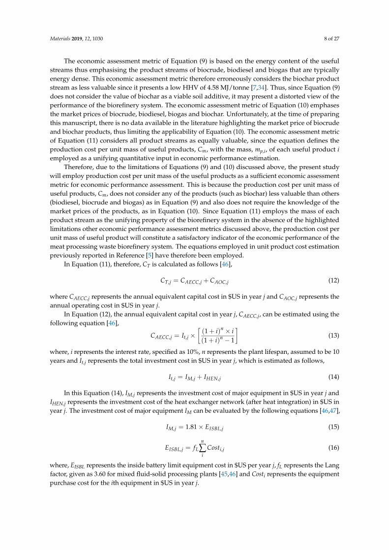
Using the ASPEN energy analyser® V.10, the composite curves, which represent the totalheating and the total cooling requirements of the biorefinery process in a cumulative manneron a temperature–enthalpy diagram, have been generated and are shown in Figure 3, based acounter-current heat exchanger network and a temperature difference of 10 ◦C. The plot employs theclassic heat integration method which is extensively described in chemical engineering textbooks andjournals [38,66,67]. It has been determined that employing 18 heat exchangers, the cooling utility andthe heating utility associated with the hot and the cold streams (Table 2) for the biorefinery process canbe reduced from 28,872.8 kW (or 103,942.1 MJ/h) and 25,621.0 kW (or 92,235.6 MJ/h) to 19,370 kW(or 69,732 MJ/h) and 16,120 kW (or 58,032 MJ/h) respectively. The pinch point temperature was alsodetermined to be 98.3 ◦C.

Materials 2019, 12, 1030 16 of 27

Materials 2019, 12, x FOR PEER REVIEW 2 of 28

H-REACT_heat 30.2 92.5 2829.8 Sum – – 25621

Using the ASPEN energy analyser® V.10, the composite curves, which represent the total heating and the total cooling requirements of the biorefinery process in a cumulative manner on a temperature–enthalpy diagram, have been generated and are shown in Figure 3, based a counter-current heat exchanger network and a temperature difference of 10 °C. The plot employs the classic heat integration method which is extensively described in chemical engineering textbooks and journals [38,66,67]. It has been determined that employing 18 heat exchangers, the cooling utility and the heating utility associated with the hot and the cold streams (Table 2) for the biorefinery process can be reduced from 28872.8 kW (or 103942.1 MJ/h) and 25621.0 kW (or 92235.6 MJ/h) to 19370 kW (or 69732 MJ/h) and 16120 kW (or 58032 MJ/h) respectively. The pinch point temperature was also determined to be 98.3 °C.

Figure 3. Composite curves for minimum driving temperature of 10 °C for the biorefinery process as generated by ASPEN energy analyser®.

The residual cooling and the heating requirements may be satisfied using cooling water and steam (generated using natural gas) as external utilities. In addition to duties associated with the hot and cold streams, additional auxiliary heating and cooling duties due to mixing heat of isothermal and isobaric separation operations were also calculated [68,69]. The total auxiliary heating duty and cooling duty in the biorefinery system were determined in ASPEN as 1,790 kW (or 64,44 MJ/h) and 447.8 kW (or 1,612 MJ/h) respectively. The electrical duty for the high pressure HTL pump has been calculated to be 386 kW (or 1389.6 MJ/h). Furthermore, as discussed in above, the combined electrical power required by the mechanical stirrers employed in the in-situ hydrolysis reactor (H-REACT), anaerobic digestion reactor (AD) and hydrothermal liquefaction reactor (HTL-R) has also estimated to be 103.1 kW (or 371.16 MJ/h). The values of the external energy duties required by the biorefinery system discussed above are summarised in Table 3 below.

In this study, only the yields of the energy dense product streams of biocrude, biodiesel and biogas of 722.5, 425.6 and 1564.3 kg/h and their associated HHVs of 36,700, 39,800 and 20,900 kJ/kg respectively are considered in calculating the total thermal energy generation potential of the biorefinery system. Applying Equation (8) above, the NER of the overall biorefinery system has been determined to be 1.010 for the case of electricity generation from fossil sources (case A) and 1.063 for the case of electricity generation from renewable sources (case B). The NER results show that for the biorefinery system in both case A and case B (NERA and NERB are greater than 1), energy recovery via the employment of the proposed biorefinery cannot result in significant positive environmental outcomes since both NER values are not substantially greater than 1.

Figure 3. Composite curves for minimum driving temperature of 10 ◦C for the biorefinery process asgenerated by ASPEN energy analyser®.

The residual cooling and the heating requirements may be satisfied using cooling water andsteam (generated using natural gas) as external utilities. In addition to duties associated with the hotand cold streams, additional auxiliary heating and cooling duties due to mixing heat of isothermaland isobaric separation operations were also calculated [68,69]. The total auxiliary heating duty andcooling duty in the biorefinery system were determined in ASPEN as 1790 kW (or 64.44 MJ/h) and447.8 kW (or 1612 MJ/h) respectively. The electrical duty for the high pressure HTL pump has beencalculated to be 386 kW (or 1389.6 MJ/h). Furthermore, as discussed in above, the combined electricalpower required by the mechanical stirrers employed in the in-situ hydrolysis reactor (H-REACT),anaerobic digestion reactor (AD) and hydrothermal liquefaction reactor (HTL-R) has also estimated tobe 103.1 kW (or 371.16 MJ/h). The values of the external energy duties required by the biorefinerysystem discussed above are summarised in Table 3 below.

In this study, only the yields of the energy dense product streams of biocrude, biodiesel andbiogas of 722.5, 425.6 and 1564.3 kg/h and their associated HHVs of 36,700, 39,800 and 20,900 kJ/kgrespectively are considered in calculating the total thermal energy generation potential of thebiorefinery system. Applying Equation (8) above, the NER of the overall biorefinery system hasbeen determined to be 1.010 for the case of electricity generation from fossil sources (case A) and 1.063for the case of electricity generation from renewable sources (case B). The NER results show that forthe biorefinery system in both case A and case B (NERA and NERB are greater than 1), energy recoveryvia the employment of the proposed biorefinery cannot result in significant positive environmentaloutcomes since both NER values are not substantially greater than 1.

Table 3. External energy duty requirements of the simulated biorefinery process.

Energy Demand Value Calculated (kW)

Heating duty

Minimum heating duty 16,120.0Auxiliary heat duty 1790.0

Total 17,910.0

Cooling duty

Minimum cooling duty 19,370.0Auxiliary cooling duty 447.8

Total 19,817.8

Electrical duty

Pumps 386.0Stirrers 103.1

Total 489.1

Materials 2019, 12, 1030 17 of 27

4.3. Economic Assessment Results

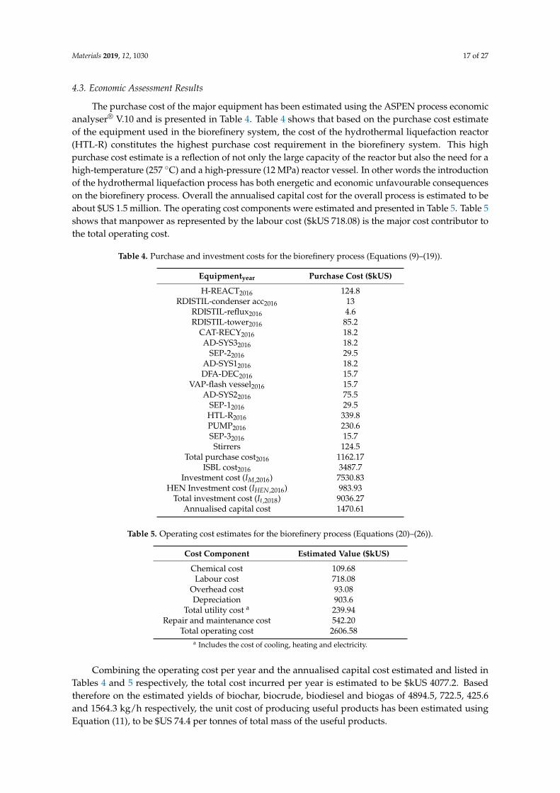
The purchase cost of the major equipment has been estimated using the ASPEN process economicanalyser® V.10 and is presented in Table 4. Table 4 shows that based on the purchase cost estimateof the equipment used in the biorefinery system, the cost of the hydrothermal liquefaction reactor(HTL-R) constitutes the highest purchase cost requirement in the biorefinery system. This highpurchase cost estimate is a reflection of not only the large capacity of the reactor but also the need for ahigh-temperature (257 ◦C) and a high-pressure (12 MPa) reactor vessel. In other words the introductionof the hydrothermal liquefaction process has both energetic and economic unfavourable consequenceson the biorefinery process. Overall the annualised capital cost for the overall process is estimated to beabout $US 1.5 million. The operating cost components were estimated and presented in Table 5. Table 5shows that manpower as represented by the labour cost ($kUS 718.08) is the major cost contributor tothe total operating cost.

Table 4. Purchase and investment costs for the biorefinery process (Equations (9)–(19)).

Equipmentyear Purchase Cost ($kUS)

H-REACT2016 124.8RDISTIL-condenser acc2016 13

RDISTIL-reflux2016 4.6RDISTIL-tower2016 85.2

CAT-RECY2016 18.2AD-SYS32016 18.2

SEP-22016 29.5AD-SYS12016 18.2DFA-DEC2016 15.7

VAP-flash vessel2016 15.7AD-SYS22016 75.5

SEP-12016 29.5HTL-R2016 339.8PUMP2016 230.6SEP-32016 15.7Stirrers 124.5

Total purchase cost2016 1162.17ISBL cost2016 3487.7

Investment cost (IM,2016) 7530.83HEN Investment cost (IHEN,2016) 983.93

Total investment cost (It,2018) 9036.27Annualised capital cost 1470.61

Table 5. Operating cost estimates for the biorefinery process (Equations (20)–(26)).

Cost Component Estimated Value ($kUS)

Chemical cost 109.68Labour cost 718.08

Overhead cost 93.08Depreciation 903.6

Total utility cost a 239.94Repair and maintenance cost 542.20

Total operating cost 2606.58a Includes the cost of cooling, heating and electricity.

Combining the operating cost per year and the annualised capital cost estimated and listed inTables 4 and 5 respectively, the total cost incurred per year is estimated to be $kUS 4077.2. Basedtherefore on the estimated yields of biochar, biocrude, biodiesel and biogas of 4894.5, 722.5, 425.6and 1564.3 kg/h respectively, the unit cost of producing useful products has been estimated usingEquation (11), to be $US 74.4 per tonnes of total mass of the useful products.

Materials 2019, 12, 1030 18 of 27

4.4. Dependence of Environmental and Economic Performance on Mass Feed Rate of Waste Streams

The effect of varying the mass feed rates of the waste streams on the economic and environmentalperformances have been initially investigated and the economic data and energetic data generatedand presented in Tables S1 and S2 respectively in the supplementary data document. Tables S1 and S2show that a constant ratio of the mass feed rate of SY waste to the mass feed rate of DAF sludge of1.019 is maintained. This implies that if the mass feed of the TMPS is known, then the mass feed rateof the DAF sludge can be determined as follows,

Mass feed rate of DAF sludge =Mass feed rate of TMPS

2.019(27)

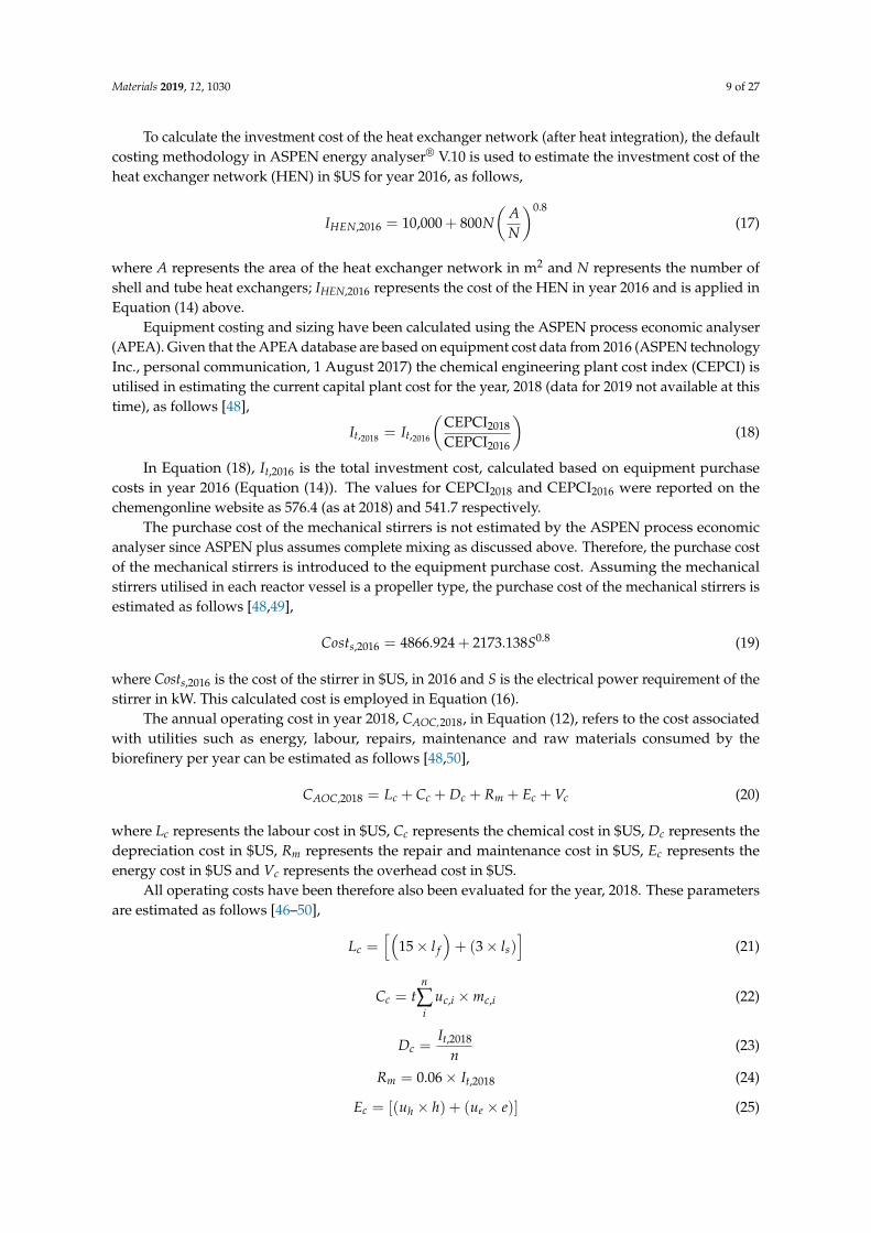
The relation presented in Equation (27) constitutes an important relation to be employed insubsequent subsections. Figures 4 and 5A,B illustrate the dependence of the unit production cost andNER, on the mass feed rate of the total meat processing waste streams (TMPS). The data employedin plotting Figures 4 and 5A,B are presented in Tables S1 and S2 respectively in the supplementarydata document.

Materials 2019, 12, x FOR PEER REVIEW 4 of 28

Annualised capital cost 1470.61

Table 5. Operating cost estimates for the biorefinery process (Equations (20)–(26)).

Cost Component Estimated Value ($kUS) Chemical cost 109.68 Labour cost 718.08

Overhead cost 93.08 Depreciation 903.6

Total utility costa 239.94 Repair and maintenance cost 542.20

Total operating cost 2606.58 a Includes the cost of cooling, heating and electricity

Combining the operating cost per year and the annualised capital cost estimated and listed in Tables 4 and 5 respectively, the total cost incurred per year is estimated to be $kUS 4,077.2. Based therefore on the estimated yields of biochar, biocrude, biodiesel and biogas of 4,894.5, 722.5, 425.6 and 1,564.3 kg/h respectively, the unit cost of producing useful products has been estimated using Equation (11), to be $US 74.4 per tonnes of total mass of the useful products.

4.4. Dependence of Environmental and Economic Performance on Mass Feed Rate of Waste Streams

The effect of varying the mass feed rates of the waste streams on the economic and environmental performances have been initially investigated and the economic data and energetic data generated and presented in Table S1 and S2 respectively in the supplementary data document. Table S1 and Table S2 show that a constant ratio of the mass feed rate of SY waste to the mass feed rate of DAF sludge of 1.019 is maintained. This implies that if the mass feed of the TMPS is known, then the mass feed rate of the DAF sludge can be determined as follows,

Mass feed rate of TMPSMass feed rate of DAF sludge = 2.019

(27)

The relation presented in Equation (27) constitutes an important relation to be employed in subsequent subsections. Figures 4 and 5A,B illustrate the dependence of the unit production cost and NER, on the mass feed rate of the total meat processing waste streams (TMPS). The data employed in plotting Figures 4 and 5A,B are presented in Tables S1 and S2 respectively in the supplementary data document.

Figure 4. Dependence of Cm on the mass feed rate of the meat processing waste streams.

Figure 4. Dependence of Cm on the mass feed rate of the meat processing waste streams.

Figures 4 and 5A,B highlight the plot of unit production cost (Cm) versus the mass feed rate of themeat processing waste streams and the plot of NER versus the mass feed rate of the meat processingwaste streams for case A (Figure 5A) and case B (Figure 5B) respectively. Figures 4 and 5A,B show thatas the mass feed rate of meat processing waste streams of DAF sludge, SY waste and mass feed rateof TPMS increases, the unit production cost reduces and the NER value increases. This observationimplies that both the environment performance and economic performance of the biorefinery systemwill benefit from larger biorefinery processing capacities, with larger mass feed rates of meat processingwaste streams leading to reduced processing cost and improved NER values in both cases A and B(discussed in Section 3.1 above). Figures 4 and 5A,B also suggest that changes in the DAF feed rate willpresent a greater effect on the unit production cost than on the NER value since the unit productioncost reduces by as much as 52% while the NER value increases by only about 1.14% (case A) and 0.46%(case B) as the mass feed rate of meat processing waste streams increases from 50% to 150% of the basecase mass feed rates. It is however not certain that the above situation of simultaneously favourableenvironmental performance will still be satisfactory if the mass feed rates DAF sludge, SY waste andTMPS are greater than 150% of their base case mass feed rates. It is therefore necessary to be furtherdetermined. Since mass feed rates DAF sludge and the SY waste can be determined from the mass feedrate of the TMPS as discussed in Section 4.1 and using Equation (27) above, the effect of increasing themass feed rates of only the TMPS to greater than 150% of the base case mass feed rate of 84.2 tonnes/h,on the NER and the unit production cost of the biorefinery system has been assessed.

Materials 2019, 12, 1030 19 of 27

Materials 2019, 12, x FOR PEER REVIEW 5 of 28

Figures 4 and 5A,B highlight the plot of unit production cost (Cm) versus the mass feed rate of

the meat processing waste streams and the plot of NER versus the mass feed rate of the meat

processing waste streams for case A (Figure 5A) and case B (Figure 5B) respectively. Figures 4 and

5A,B show that as the mass feed rate of meat processing waste streams of DAF sludge, SY waste and

mass feed rate of TPMS increases, the unit production cost reduces and the NER value increases.

This observation implies that both the environment performance and economic performance of the

biorefinery system will benefit from larger biorefinery processing capacities, with larger mass feed

rates of meat processing waste streams leading to reduced processing cost and improved NER

values in both cases A and B (discussed in Section 3.1 above). Figures 4 and 5A,B also suggest that

changes in the DAF feed rate will present a greater effect on the unit production cost than on the

NER value since the unit production cost reduces by as much as 52% while the NER value increases

by only about 1.14% (case A) and 0.46% (case B) as the mass feed rate of meat processing waste

streams increases from 50% to 150% of the base case mass feed rates. It is however not certain that

the above situation of simultaneously favourable environmental performance will still be

satisfactory if the mass feed rates DAF sludge, SY waste and TMPS are greater than 150% of their

base case mass feed rates. It is therefore necessary to be further determined. Since mass feed rates

DAF sludge and the SY waste can be determined from the mass feed rate of the TMPS as discussed

in Section 4.1 and using Equation (27) above, the effect of increasing the mass feed rates of only the

TMPS to greater than 150% of the base case mass feed rate of 84.2 tonnes/h, on the NER and the unit

production cost of the biorefinery system has been assessed.

(A)

(B)

Figure 5. Dependence of NER, energy demand and energy potential on the mass feed rate of the total

meat processing waste stream. (A) for case when electrical energy is generated from fossil sources

and (B) for case when electrical energy is generated from renewable energy sources. Slight numerical

fluctuations are responsible for the lack of perfect smoothness in NER versus the total meat

processing waste stream (B).

[A]

[B]

35

45

55

65

75

85

95

105

115

125

1.000

1.002

1.004

1.006

1.008

1.010

1.012

1.014

1.016

40 50 60 70 80 90 100 110 120 130

En

ergy

(GJ/

h)

NE

R

Mass feed rate (tonnes/h)

NER Energy demand (GJ/h) Energy potential (GJ/h)

35

45

55

65

75

85

95

105

115

125

1.059

1.060

1.061

1.062

1.063

1.064

1.065

40 50 60 70 80 90 100 110 120 130

En

ergy

(GJ/

h)

NE

R

Mass feed rate (tonnes/h)

NER Energy demand (GJ/h) Energy potential (GJ/h)

[A]

[B]

35

45

55

65

75

85

95

105

115

125

1.000

1.002

1.004

1.006

1.008

1.010

1.012

1.014

1.016

40 50 60 70 80 90 100 110 120 130

En

ergy

(GJ/

h)

NE

R

Mass feed rate (tonnes/h)

NER Energy demand (GJ/h) Energy potential (GJ/h)

35

45

55

65

75

85

95

105

115

125

1.059

1.060

1.061

1.062

1.063

1.064

1.065

40 50 60 70 80 90 100 110 120 130

En

ergy

(GJ/

h)

NE

R

Mass feed rate (tonnes/h)

NER Energy demand (GJ/h) Energy potential (GJ/h)

Figure 5. Dependence of NER, energy demand and energy potential on the mass feed rate of the totalmeat processing waste stream. (A) for case when electrical energy is generated from fossil sourcesand (B) for case when electrical energy is generated from renewable energy sources. Slight numericalfluctuations are responsible for the lack of perfect smoothness in NER versus the total meat processingwaste stream (B).

The NER and the unit production cost of the biorefinery system have therefore been furtherinvestigated for several mass feed rates of TMPS of 161.5 tonnes/h (A), 242.3 tonnes/h (B) and282.7 tonnes/h (C) which are all greater than 150% of the base case mass feed rate of 126.2 tonnes/h.The modelled results from ASPEN plus are presented in Tables S3 and S4 in the supplementary datadocument and the data used in generating plots showing the dependence of the unit production cost,Cm and NER on the mass feed rate of TMPS as shown in Figures 6 and 7A,B respectively. Figures 6and 7A,B show that when the mass feed rates of the TMPS are 161.5 tonnes/h, 242 tonnes/h and282.7 tonnes/h, corresponding to points A, B and C on the respective plots, the same trend as shown inFigure 6 is observed with the unit production cost, Cm, reduced to $US 53.39/tonne, $US 44.76/tonneand then $US 42.48/tonne as the mass feed rate of TMPS increases further from 161.5 tonnes to242 tonnes and then 282.7 tonnes respectively. However Figure 7A,B show different trends from thetrends shown in Figure 7A,B for NER is shown, with Figure 7A showing that the NER reduces from1.010 to 0.988 and then 0.986 as the mass feed rates of the TMPS further increases from 161.5 to 242 andthen 282.7 tonnes. Figure 7B also shows that the NER reduces from 1.059 to 1.033 and then 1.030 as themass feed rates of the TMPS further increases from 161.5 to 242 and then 282.7 tonnes.

Materials 2019, 12, 1030 20 of 27

Materials 2019, 12, x FOR PEER REVIEW 6 of 28

The NER and the unit production cost of the biorefinery system have therefore been further

investigated for several mass feed rates of TMPS of 161.5 tonnes/h (A), 242.3 tonnes/h (B) and 282.7

tonnes/h (C) which are all greater than 150% of the base case mass feed rate of 126.2 tonnes/h. The

modelled results from ASPEN plus are presented in Tables S3 and S4 in the supplementary data

document and the data used in generating plots showing the dependence of the unit production

cost, Cm and NER on the mass feed rate of TMPS as shown in Figures 6 and 7A,B respectively.

Figures 6 and 7A,B show that when the mass feed rates of the TMPS are 161.5 tonnes/h, 242 tonnes/h

and 282.7 tonnes/h, corresponding to points A, B and C on the respective plots, the same trend as

shown in Figure 6 is observed with the unit production cost, Cm, reduced to $US53.39/tonne,

$US44.76/tonne and then $US42.48/tonne as the mass feed rate of TMPS increases further from 161.5

tonnes to 242 tonnes and then 282.7 tonnes respectively. However Figure 7A,B show different trends

from the trends shown in Figure 7A,B for NER is shown, with Figure 7A showing that the NER

reduces from 1.010 to 0.988 and then 0.986 as the mass feed rates of the TMPS further increases from

161.5 to 242 and then 282.7 tonnes. Figure 7B also shows that the NER reduces from 1.059 to 1.033 and

then 1.030 as the mass feed rates of the TMPS further increases from 161.5 to 242 and then 282.7

tonnes.

Figure 6. Variation of the unit production cost with the mass feed rates. Points A, B and C represent

mass feed rates of TMPS that are 192%, 288% and 336% (all greater than 150%) of the base case TMPS

mass feed rate of 84.2 tonnes/h.

Figure 6 shows that a larger mass feed rate of the waste streams will always lead to a reduced

unit production cost, with the production cost reducing asymptotically towards a possible constant

value. In other words in the absence of the environmental performance consideration, increasing the

mass feed rate of the waste streams processed by the biorefinery system will constitute the logical

approach to enhance the economic performance. Figure 7A,B however show that with an increase in

the mass feed rate of the waste streams the NER increase initially, peak and then begin to

deteriorate.

(A)

AB C

0

20

40

60

80

100

120

140

40 90 140 190 240 290

Cm

($U

S/

ton

ne)

Mass feed rate (tonnes/h)

[A]

[B]

A

B C

0.980

0.985

0.990

0.995

1.000

1.005

1.010

1.015

1.020

40 90 140 190 240 290

NE

R

Mass feed rate (tonnes/h)

A

BC

1.025

1.030

1.035

1.040

1.045

1.050

1.055

1.060

1.065

1.070

40 90 140 190 240 290

NE

R

Mass feed rate (tonnes/h)

Figure 6. Variation of the unit production cost with the mass feed rates. Points A, B and C representmass feed rates of TMPS that are 192%, 288% and 336% (all greater than 150%) of the base case TMPSmass feed rate of 84.2 tonnes/h.

Figure 6 shows that a larger mass feed rate of the waste streams will always lead to a reduced unitproduction cost, with the production cost reducing asymptotically towards a possible constant value.In other words in the absence of the environmental performance consideration, increasing the massfeed rate of the waste streams processed by the biorefinery system will constitute the logical approachto enhance the economic performance. Figure 7A,B however show that with an increase in the massfeed rate of the waste streams the NER increase initially, peak and then begin to deteriorate.

Materials 2019, 12, x FOR PEER REVIEW 6 of 28

The NER and the unit production cost of the biorefinery system have therefore been further

investigated for several mass feed rates of TMPS of 161.5 tonnes/h (A), 242.3 tonnes/h (B) and 282.7

tonnes/h (C) which are all greater than 150% of the base case mass feed rate of 126.2 tonnes/h. The

modelled results from ASPEN plus are presented in Tables S3 and S4 in the supplementary data

document and the data used in generating plots showing the dependence of the unit production

cost, Cm and NER on the mass feed rate of TMPS as shown in Figures 6 and 7A,B respectively.

Figures 6 and 7A,B show that when the mass feed rates of the TMPS are 161.5 tonnes/h, 242 tonnes/h

and 282.7 tonnes/h, corresponding to points A, B and C on the respective plots, the same trend as

shown in Figure 6 is observed with the unit production cost, Cm, reduced to $US53.39/tonne,

$US44.76/tonne and then $US42.48/tonne as the mass feed rate of TMPS increases further from 161.5

tonnes to 242 tonnes and then 282.7 tonnes respectively. However Figure 7A,B show different trends

from the trends shown in Figure 7A,B for NER is shown, with Figure 7A showing that the NER

reduces from 1.010 to 0.988 and then 0.986 as the mass feed rates of the TMPS further increases from

161.5 to 242 and then 282.7 tonnes. Figure 7B also shows that the NER reduces from 1.059 to 1.033 and

then 1.030 as the mass feed rates of the TMPS further increases from 161.5 to 242 and then 282.7

tonnes.

Figure 6. Variation of the unit production cost with the mass feed rates. Points A, B and C represent

mass feed rates of TMPS that are 192%, 288% and 336% (all greater than 150%) of the base case TMPS

mass feed rate of 84.2 tonnes/h.

Figure 6 shows that a larger mass feed rate of the waste streams will always lead to a reduced

unit production cost, with the production cost reducing asymptotically towards a possible constant

value. In other words in the absence of the environmental performance consideration, increasing the

mass feed rate of the waste streams processed by the biorefinery system will constitute the logical

approach to enhance the economic performance. Figure 7A,B however show that with an increase in

the mass feed rate of the waste streams the NER increase initially, peak and then begin to

deteriorate.

(A)

AB C

0

20

40

60

80

100

120

140

40 90 140 190 240 290

Cm

($U

S/

ton

ne)

Mass feed rate (tonnes/h)

[A]

[B]

A

B C

0.980

0.985

0.990

0.995

1.000

1.005

1.010

1.015

1.020

40 90 140 190 240 290

NE

R

Mass feed rate (tonnes/h)

A

BC

1.025

1.030

1.035

1.040

1.045

1.050

1.055

1.060

1.065

1.070

40 90 140 190 240 290

NE

R

Mass feed rate (tonnes/h)

Materials 2019, 12, x FOR PEER REVIEW 7 of 28

(B)

Figure 7. Variation of the NER with the mass feed rates. Points A, B and C represent mass feed rates

of TMPS that are 192%, 288% and 336% (all greater than 150%) of the base case TMPS mass feed rate

of 84.2 tonnes/h. (A): Case A and (B): case B.

This indicates that at a high mass feed rate of the TMPS the energy cost necessary for processing

of the waste streams to useful products will exceed the energy potential of the energy dense product

streams of biodiesel, biocrude and biogas leading to poorer environmental performance (i.e., lower

NER). To determine the most acceptable feed rate of the TMPS, for the best compromise

performances for NER and unit production cost (Section 4.1), it is necessary to establish the relations

between the mass feed rates of TMPS and the NER and the relation between the mass feed rates of

TMPS and the unit production cost.

A least square regression line fitting method [70] in JMP® statistical software version 10.0.0 (SAS

Institute Inc., Cary, NC, USA) has been employed to develop relevant fitted relations. For the mass

feed rate of TMPS ranging from 42 tonne/h to 282.7 tonnes/h, the following two fitted relations for

the unit production cost (Cm) and the NER for case A (NERA) and case B (NERB) have been

established respectively, as follows,

( ) ( ) ( ) ( )

( )

5 4 3 210 7 4 29.68 10 8.72 10 3.05 10 5.26 10

4.70 238.89

mC m m m m

m

− − − −= − + − +

− + (28)

and

( ) ( ) ( ) ( )

( ) ( )

6 5 4 314 12 9 7

A

25 3

NER 1.03 10 9.8 10 3.59 10 6.4 10

6.06 10 3.01 10 0.9449

m m m m

m m

− − − −

− −

= − + − +

− + + (29)

( ) ( ) ( ) ( )

( ) ( )

6 5 4 314 11 9 7

B

25 3

NER 1.1 10 1 10 3.64 10 6.37 10

5.77 10 2.64 10 1.013

m m m m

m m

− − − −

− −

= − + − +

− + + (30)

In the three equations above, m is the mass feed rate of TMPS in tonnes/h and ranging from 42

to 282.7 tonnes/h. The coefficient of determination (R2) for Equations (28)–(30) are 0.9992, 0.9997 and

0.9998, respectively. The three relations are shown in Figures 6 and 7A,B, as the dashed curves for

unit production cost (Cm) versus mass feed rate plot and NER versus mass feed rate plot respectively.

Utilising the fitted relations presented in Equations (28)–(30) above and the JMP software for

desirability optimisation as discussed in Section 4.1 above, the mass flow rate of TMPS, that will

provide a best compromise trade-off between the competing NER and the unit production cost, Cm,

has been determined and presented in Table 6. Table 6 also shows that for case B, the mass feed rate

of TMPS that will enable the best compromise between competing NER and unit production cost, Cm

is 140.8 tonnes/h with the associated NER and unit production cost, Cm of 1.063 and $US 57.0 per

tonne respectively. Employing Equation (27) above, in both cases, A and B, the mass feed rate of

DAF sludge can be estimated to be 71.62 and 69.74 tonnes/h respectively. Given that the ratio of the

[A]

[B]

A

B C

0.980

0.985

0.990

0.995

1.000

1.005

1.010

1.015

1.020

40 90 140 190 240 290

NE

R

Mass feed rate (tonnes/h)

A

BC

1.025

1.030

1.035

1.040

1.045

1.050

1.055

1.060

1.065

1.070

40 90 140 190 240 290

NE

R

Mass feed rate (tonnes/h)

Figure 7. Variation of the NER with the mass feed rates. Points A, B and C represent mass feed rates ofTMPS that are 192%, 288% and 336% (all greater than 150%) of the base case TMPS mass feed rate of84.2 tonnes/h. (A): Case A and (B): case B.

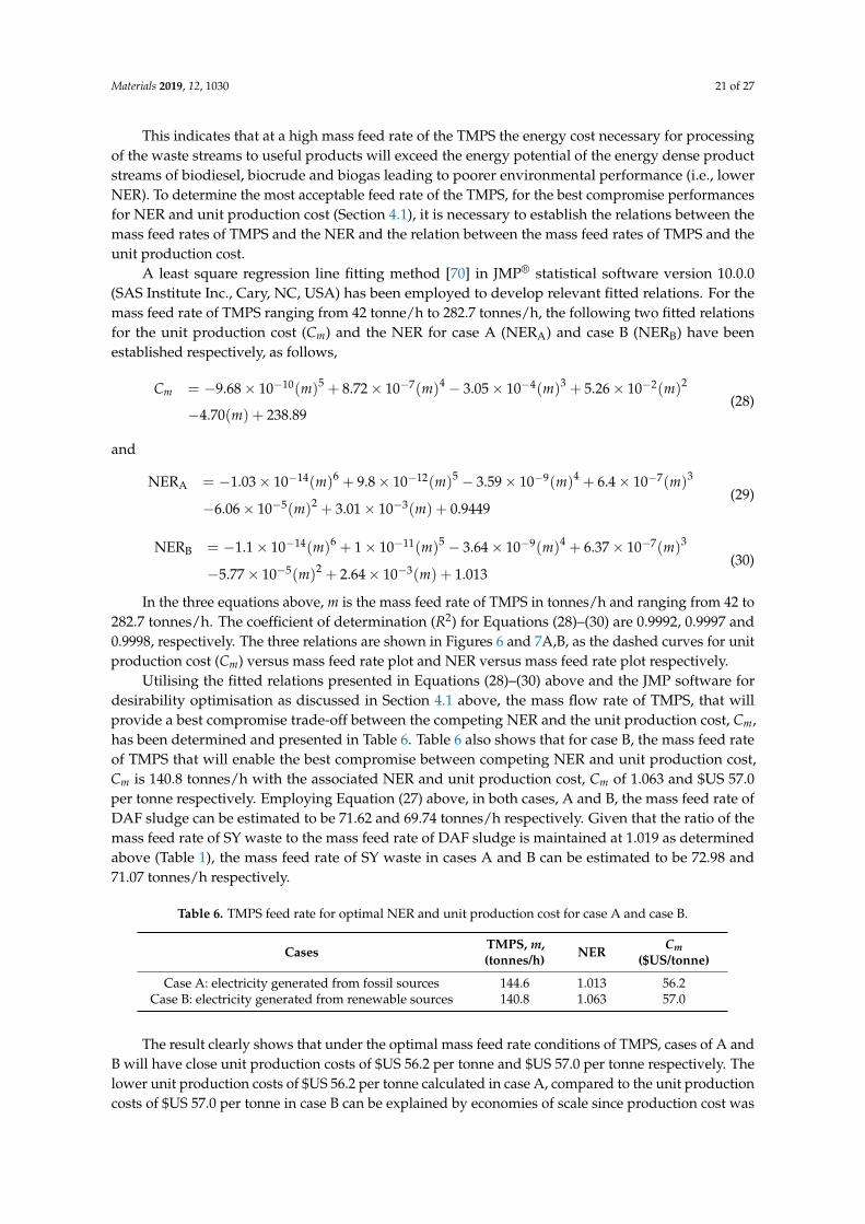
Materials 2019, 12, 1030 21 of 27

This indicates that at a high mass feed rate of the TMPS the energy cost necessary for processingof the waste streams to useful products will exceed the energy potential of the energy dense productstreams of biodiesel, biocrude and biogas leading to poorer environmental performance (i.e., lowerNER). To determine the most acceptable feed rate of the TMPS, for the best compromise performancesfor NER and unit production cost (Section 4.1), it is necessary to establish the relations between themass feed rates of TMPS and the NER and the relation between the mass feed rates of TMPS and theunit production cost.

A least square regression line fitting method [70] in JMP® statistical software version 10.0.0(SAS Institute Inc., Cary, NC, USA) has been employed to develop relevant fitted relations. For themass feed rate of TMPS ranging from 42 tonne/h to 282.7 tonnes/h, the following two fitted relationsfor the unit production cost (Cm) and the NER for case A (NERA) and case B (NERB) have beenestablished respectively, as follows,

Cm = −9.68× 10−10(m)5 + 8.72× 10−7(m)4 − 3.05× 10−4(m)3 + 5.26× 10−2(m)2

−4.70(m) + 238.89(28)

and

NERA = −1.03× 10−14(m)6 + 9.8× 10−12(m)5 − 3.59× 10−9(m)4 + 6.4× 10−7(m)3

−6.06× 10−5(m)2 + 3.01× 10−3(m) + 0.9449(29)

NERB = −1.1× 10−14(m)6 + 1× 10−11(m)5 − 3.64× 10−9(m)4 + 6.37× 10−7(m)3

−5.77× 10−5(m)2 + 2.64× 10−3(m) + 1.013(30)

In the three equations above, m is the mass feed rate of TMPS in tonnes/h and ranging from 42 to282.7 tonnes/h. The coefficient of determination (R2) for Equations (28)–(30) are 0.9992, 0.9997 and0.9998, respectively. The three relations are shown in Figures 6 and 7A,B, as the dashed curves for unitproduction cost (Cm) versus mass feed rate plot and NER versus mass feed rate plot respectively.

Utilising the fitted relations presented in Equations (28)–(30) above and the JMP software fordesirability optimisation as discussed in Section 4.1 above, the mass flow rate of TMPS, that willprovide a best compromise trade-off between the competing NER and the unit production cost, Cm,has been determined and presented in Table 6. Table 6 also shows that for case B, the mass feed rateof TMPS that will enable the best compromise between competing NER and unit production cost,Cm is 140.8 tonnes/h with the associated NER and unit production cost, Cm of 1.063 and $US 57.0per tonne respectively. Employing Equation (27) above, in both cases, A and B, the mass feed rate ofDAF sludge can be estimated to be 71.62 and 69.74 tonnes/h respectively. Given that the ratio of themass feed rate of SY waste to the mass feed rate of DAF sludge is maintained at 1.019 as determinedabove (Table 1), the mass feed rate of SY waste in cases A and B can be estimated to be 72.98 and71.07 tonnes/h respectively.

Table 6. TMPS feed rate for optimal NER and unit production cost for case A and case B.

Cases TMPS, m,(tonnes/h) NER Cm

($US/tonne)

Case A: electricity generated from fossil sources 144.6 1.013 56.2Case B: electricity generated from renewable sources 140.8 1.063 57.0

The result clearly shows that under the optimal mass feed rate conditions of TMPS, cases of A andB will have close unit production costs of $US 56.2 per tonne and $US 57.0 per tonne respectively. Thelower unit production costs of $US 56.2 per tonne calculated in case A, compared to the unit productioncosts of $US 57.0 per tonne in case B can be explained by economies of scale since production cost was

Materials 2019, 12, 1030 22 of 27

shown to reduce as the mass of the feed rate of the TMPS increased (Figure 6 above). Case A and caseB have also been initially shown to constitute environmentally sustainable processes since their NERsare 1.013 and 1.063 respectively and both NERs are greater than 1.

This preliminary assessment also suggests that assuming the meat processing waste streams ofSY waste and DAF sludge are readily available on site, such that the transportation cost is negligible, asingle large capacity biorefinery plant (TMPS of 144.6 tonnes/h, case A and 140.8 tonnes/h, case B)to satisfy the resource recovery needs of a particular region will be preferred to the installation ofseveral smaller capacity biorefinery plants in that region, from a perspective of both environmentalperformance and economic performance. However, in the absence of sufficient meat processing wastestreams of SY waste and DAF sludge in a particular region, cost escalation due to the transportationwaste streams over long distances may limit the long term viability of such a large capacity biorefineryplant. This is because such cost escalations may increase the unit production cost well beyond thecosting range and scope considered in this study.

4.5. Unit Production Cost Comparison with Data Obtained from Peer-Reviewed Literature

To provide a context for the assessment of the economic performance of the optimised biorefinerysystem, unit production costs of valuable products of biochar, biocrude, biogas and biodiesel havebeen compared to unit production costs of the respective products. Employing the determined massflow rate of TMPS of 144.6 tonnes/h (DAF: 71.62 tonnes/h, SY: 72.98 tonnes/h) and 140.8 tonnes/h(DAF: 69.74 tonnes/h, SY: 71.07 tonnes/h) for case A and case B respectively, the mass (tonnes) ofthe valuable products produced per h can be calculated in ASPEN plus by undertaking the samesimulation steps highlighted in Sections 3 and 4 above. The mass of the useful products from thebiorefinery in case A and case B are therefore summarised in Table 7.

Table 7. Mass flow rate of useful products from the proposed biorefinery system.

BiorefinerySystem

Production Cost(US$/year)

Mass Flow Rate of Valuable Products (tonnes/h)

Biogas Biocrude Biodiesel Biochar

Case A 5291962.85 2.698 1.241 0.734 8.405Case B 5226156.72 2.627 1.208 0.715 8.184

Table 7 shows the mass flow rate of the valuable products and annual production costs for cases Aand B of the biorefinery such that the unit production costs of each of the products is calculated and theresults summarised in Table 8. Table 8 shows the production costs of useful products per unit mass andper unit volume. The conversion of the unit production cost from a mass basis to a volumetric basishas been achieved by multiplying production costs per unit mass of each product by their respectivedensities. These densities are specified as 0.0012 kg/L [71], 0.8692 kg/L [4], 0.974 kg/L [7,34] and0.51 kg/L (bulk density) [72] for biogas, biodiesel, biocrude and biochar respectively.

Table 8. Mass flow rate of useful products from the proposed biorefinery system.

Biorefinery System Unit Production Cost Biogas Biocrude Biodiesel Biochar

Case AUS$/kg 0.2724 0.5923 1.0009 0.0874US$/L 0.00031 0.5610 0.870 0.0446

Case BUS$/kg 0.2763 0.6008 1.0152 0.0887US$/L 0.00032 0.5690 0.8824 0.0452

A review of the literature shows that the unit production costs of biocrude, biochar (from waste)and biodiesel are US$ 0.85/L [73], US$ 0.26/L [74] and US$ 1.124/L (mean) [75–77] respectively.Since the mean production cost for biogas is approximately €14 per GJ of biogas heat content [78],the production cost of biogas per L can be estimated from the knowledge of its HHV and density

Materials 2019, 12, 1030 23 of 27

of 20.9 MJ/kg [6] and 0.00115 kg/L [71] respectively. The mean unit production cost of biogas iscalculated to be €0.00025/L which is equivalent to US$ 0.00029/L, based on the prevailing currencyexchange rate of €1 to US$ 1.17 (assessed on the 14th of September 2018 from www.currency-calc.com).

Comparing the literature on the obtained unit production costs and the unit production costsobtained from the present study for products of biodiesel, biocrude and biochar, it is clear that theproposed biorefinery system can generate the aforementioned useful products with comparativelyreduced unit production costs relative to the current unit production costs of the products found in theliterature. The unit production costs of the biogas, in both cases A and B, were however estimatedto be US$ 0.00031/L and US$ 0.00032/L which are comparable to the literature obtained currentmean unit production cost of biogas of US$ 0.00029/L. The ability of the biorefinery to generateuseful products at lower unit production costs relative to the literature obtained unit productioncosts of the independently produced respective products may be largely due to the generation ofmultiple product streams from the proposed biorefinery system. This observation is consistent with aprevious study in which it was shown that the production of a single useful product may not constitutethe most economically favourable approach for organic waste utilisation, with the production ofmultiple useful product streams from an organic waste feedstock preferred for improved economicperformance [79]. It is therefore clear that the proposed meat processing waste biorefinery enables therecovery of useful products of biodiesel, biocrude and biochar from meat processing waste at reducedunit production costs.

5. Conclusions

This study has presented an assessment of the economic performance and environmentalperformance of the proposed large-scale meat processing waste biorefinery system for the recovery ofvaluable materials and for the production of valuable products: biocrude, biodiesel and biogas products(biofuels) and biochar (biomaterial). In this study, two cases, A and B—denoting systems in whichelectricity generation employs fossil energy sources and renewable energy sources respectively—havebeen investigated. It was demonstrated that some synergy initially exists between the economicperformance and environmental performance of the biorefinery system as the mass flow rate of themeat processing waste stream increases. The model results show that an increase in the mass feedrate of the meat processing waste from 50% to 150% of the base case mass feed rate has positiveeffects on economic and environmental performance. The positive effect of increasing the mass flowrates of the meat processing waste stream on economic performance is shown to be greater than thepositive effect on environmental performance. This is because the increase in the mass feed rate ofmeat processing waste stream from 50% to 150% of the base case mass feed rate of the waste streamresulted in a 1.14% and 0.46% improvement in environmental performance in case A and case Brespectively while a 52% improvement in economic performance was determined. However, a furtherincrease in the mass feed rates of the meat processing waste to 192%, 288% and 336% of the basecase mass feed rate, was observed to lead to a deterioration in environmental performance in bothcases A and B. The total mass feed rate of the waste stream that resulted in a satisfactory compromisebetween the competing environmental performance and economic performance was determined tobe 144.6 and 140.8 tonnes/h in cases A and B respectively. This high value of the mass feed rate inboth cases suggests that a biorefinery system with a large capacity could be preferable to smallerones from both economic and environmental perspectives, provided of course that the waste streamsare readily available in close proximity to the biorefinery system and therefore reduce the risk oftransportation cost escalation. Most importantly this study was able to show that when the determinedcompromise mass flow rates of the meat processing waste stream in cases A and B are processedby the biorefinery system, a reduction in the unit production cost of biocrude, biodiesel (biofuels)and biochar (biomaterial) was feasible without sacrificing the need for environmental sustainability.The unit production cost of biogas (biofuel) was however shown to be comparable to the existing unitproduction cost of biogas, according to the literature.

Materials 2019, 12, 1030 24 of 27

Supplementary Materials: The following are available online at http://www.mdpi.com/1996-1944/12/7/1030/s1,Table S1: The major costing components calculated for different feedstock mass feed rate scenarios, Table S2:Energy input, energy potential and mass flow rate of useful products generated for different feedstock mass feedrate scenarios, Table S3: The major costing components calculated for different TMPS mass feed rates, Table S4:Energy input, energy potential and mass flow rate of useful products generated for different TMPS mass feedrates for case A and Case B.

Author Contributions: Conceptualization, Z.S. and J.B.; Methodology, O.V.O.; Software, O.V.O.; Validation, Z.S.and J.B.; Writing–Original Draft Preparation, O.V.O.; Writing–Review & Editing, O.V.O., Z.S. and J.B.

Funding: This research received no external funding.

Acknowledgments: Oseweuba gratefully acknowledges the financial support of the University of Otago via theOtago Doctoral scholarship.

Conflicts of Interest: The authors declare no conflict of interest.

References

1. Okoro, O.V.; Sun, Z.; Birch, J. Meat processing waste as a potential feedstock for biochemicals and biofuels-A review of possible conversion technologies. J. Clean. Prod. 2017, 142, 1583–1608. [CrossRef]

2. Sadhukhan, J.; Lloyd, J.R.; Scott, K.; Premier, G.C.; Yu, E.H.; Curtis, T.; Head, I.M. A critical review ofintegration analysis of microbial electrosynthesis (MES) systems with waste biorefineries for the productionof biofuel and chemical from reuse of CO2. Renew. Sustain. Energy Rev. 2016, 56, 116–132. [CrossRef]

3. Okoro, O.; Sun, Z.; Birch, J. Experimental evaluation of a polystyrene sulphonic acid resin catalyst inthe hydrolysis of low-grade lipids from the meat processing industry. Biomass Bioenergy 2018, 116, 49–59.[CrossRef]

4. Okoro, O.V.; Sun, Z.; Birch, J. Meat processing dissolved air flotation sludge as a potential biodiesel feedstockin New Zealand: A predictive analysis of the biodiesel product properties. J. Clean. Prod. 2017, 168, 1436–1447.[CrossRef]

5. Okoro, O.V. Scaled-up biodiesel production from meat processing dissolved air flotation sludge: A simulationstudy. AgriEngineering 2018, 1, 17–43. [CrossRef]

6. Okoro, O.V.; Sun, Z.; Birch, J. Prognostic assessment of the viability of hydrothermal liquefaction as apost-resource recovery step after enhanced biomethane generation using co-digestion technologies. Appl. Sci.2018, 8, 2290. [CrossRef]

7. Okoro, V.O.; Zhifa, S.; Birch, J. Thermal depolymerisation of digestate for biofuel and biomaterial production.In Proceedings of the 4th World Congress on New Technologies (NewTech’18), Madrid, Spain, 19–21August 2018.

8. Okoro, V.O.; Zhifa, S.; Birch, J. Thermal de-polymerization of biogas digestate as a viable digestate processingand resource recovery strategy. In Advances in Eco-Fuels for Sustainable Development; Kalam Azad, Ed.;Woodhead Publishing: Cambridge, UK, 2019; pp. 227–304.

9. Luyben, W.L.; Chien, I.-L. Steady-State Design in Aspen Plus. In Design and Control of Distillation Systems forSeparating Azeotropes; John Wiley & Sons Inc.: Hoboken, NJ, USA, 2010.

10. Schefflan, R. Teach Yourself the Basics of Aspen Plus™; John Wiley & Sons: Cambridge, UK, 2011.11. Aspentech. ASPEN Plus; Aspentech: Burlington, NJ, USA, 2011.12. Zong, L.; Ramanathan, S.; Chen, C. Fragment-Based Approach for Estimating Thermophysical Properties of

Fats and Vegetable Oils for Modeling Biodiesel Production Processes. Ind. Eng. Chem. Res. 2010, 49, 876–886.[CrossRef]

13. Song, C.; Liu, Q.; Ji, N.; Deng, S.; Zhao, J.; Li, S.; Kitamura, Y. Evaluation of hydrolysis–esterification biodieselproduction from wet microalgae. Bioresour. Technol. 2016, 214, 747–754. [CrossRef]

14. Saylor. Carbohydrates. 2010. Available online: https://www.saylor.org/site/wp-content/uploads/2010/11/BIO101-Carbohydrates.pdf (accessed on 27 October 2017).

15. ASPEN. ASPEN Plus User Guide; Aspen Technology, Inc.: Cambridge, UK, 2000.16. Patel, A.; Brahmkhatri, V. Kinetic study of oleic acid esterification over 12-tungstophosphoric acid catalyst

anchored to different mesoporous silica supports. Fuel Process. Technol. 2013, 113, 141–149. [CrossRef]17. Oh, S.T.; Martin, A.D. Thermodynamic equilibrium model in anaerobic digestion process. Biochem. Eng. J.

2007, 34, 256–266. [CrossRef]

Materials 2019, 12, 1030 25 of 27

18. Basu, P. Biomass Gasification and Pyrolysis: Practical Design and Theory; Academic Press: Burington, NJ,USA, 2010.

19. Sreejith, C.C.; Muraleedharan, C.; Arun, P. Thermo-Chemical Analysis of Biomass Gasification by GibbsFree Energy Minimization Model-Part: II (Optimization of Biomass Feed and Steam to Biomass Ratio). Int. J.Green Energy 2013, 10, 610–639. [CrossRef]

20. Milani, M.; Montorsi, L.; Stefani, M. An integrated approach to energy recovery from biomass and waste:Anaerobic digestion–gasification–water treatment. Waste Manag. Res. 2014, 32, 614–625. [CrossRef]

21. Hoffmann, J.; Rudra, S.; Toor, S.S.; Holm-Nielsen, J.B.; Rosendahl, L.A. Conceptual design of an integratedhydrothermal liquefaction and biogas plant for sustainable bioenergy production. Bioresour. Technol. 2013,129, 402–410. [CrossRef]

22. Salman, C.A.; Schwede, S.; Thorina, E.; Yana, J. Predictive modelling and simulation of integrated pyrolysisand anaerobic digestion process. Energy Procedia 2017, 105, 850–857. [CrossRef]

23. Martínez-Ruano, J.A.; Caballero-Galván, A.S.; Restrepo-Serna, D.L.; Cardona, C.A. Techno-economic andenvironmental assessment of biogas production from banana peel (Musa paradisiaca) in a biorefinery concept.Environ. Sci. Pollut. Res. 2018, 25, 35971–35980. [CrossRef] [PubMed]

24. Oreggioni, G.D.; Gowreesunker, B.L.; Tassou, S.A.; Bianchi, G.; Reilly, M.; Kirby, M.E.; Toop, T.A.;Theodorou, M.K. Potential for Energy Production from Farm Wastes Using Anaerobic Digestion in theUK: An Economic Comparison of Different Size Plants. Energies 2017, 10, 1396. [CrossRef]

25. Raposo, F.; Fernández-Cegrí, V.; De la Rubia, V.; Borja, R.; Béline, F.; Cavinato, C.; Demirer, G.; Fernández, B.;Fernández-Polanco, M.; Frigon, J.C.; et al. Biochemical methane potential (BMP) of solidorganic substrates:Evaluation of anaerobicbiodegradability using data from an international interlaboratory study. J. Chem.Technol. Biotechnol. 2011, 86, 1088–1098. [CrossRef]

26. Nielfa, A.; Cano, R.; Fdz-Polanco, M. Theoretical methane production generated by the co-digestion oforganic fraction municipal solid waste and biological sludge. Biotechnol. Rep. 2015, 5, 14–21. [CrossRef][PubMed]

27. Achinas, S.; Euverink, G.J.W. Theoretical analysis of biogas potential prediction from agricultural waste.Resour.-Effic. Technol. 2016, 2, 143–147. [CrossRef]

28. Fogacs, G. Biogas Production from Citrus Wastes and Chicken Feather: Pretreatment and Co-Digestion.Ph.D. Thesis, Chalmers University of Technology, Göteborg, Sweden, 2012.

29. Valdez, P.; Tocco, V.; Savage, P. A general kinetic model for the hydrothermal liquefaction of microalgae.Bioresour. Technol. 2014, 163, 123–127. [CrossRef] [PubMed]

30. Johnson, R.S. Hydrothermal Processing of Biomass and Related Model Compounds. Ph.D. Thesis, Universityof Leeds Energy Research Institute, Leeds, UK, 2012.

31. Mørup, A.; Becker, J.; Christensen, P.; Houlberg, K.; Lappa, E.; Klemmer, M.; Madsen, R.; Glasius, M.;Iversen, B. Construction and commisioning of a continuous reactor for hydrothermal liquefaction. Ind. Chem.Eng. Res. 2015, 54, 5935–5947. [CrossRef]

32. Madsen, R.; Christensen, P.; Houlberg, K.; Lappa, E.; Mørup, A.; Klemmer, M.; Olsen, E.; Jensen, M.; Becker, J.;Iversen, B.; et al. Analysis of organic gas phase compounds formed by hydrothermal liquefaction of DriedDistillers Grains with Solubles. Bioresour. Technol. 2015, 192, 826–830. [CrossRef] [PubMed]

33. Nan, W.; Shende, A.R.; Shannon, J.; Shende, R.V. Insight into catalytic hydrothermal liquefaction of cardboardfor biofuels production. Energy Fuels 2016, 30, 4933–4944. [CrossRef]

34. Okoro, O.V.; Zhifa, S.; Birch, J. Thermal Depolymerisation of Digestate for the Optimal Co-Generation of a LiquidFuel and an Agricultural Soil Enhancer; International conference on energy research: Madrid, Spain, 2018.

35. Carlson, E. Don’t gamble with physical properties for simulations. Chem. Eng. Prog. 1996, 92, 35–46.36. Edwards, E.J. Process Modelling Selection of Thermodynamic Methods. 2008. Available online: https://

www.chemstations.com/content/documents/Technical_Articles/thermo.pdf (accessed on 22 January 2019).37. Aspen. Aspen Physical Property System: Physical Property Models; Aspen tech: Cambridge, UK, 2012.38. Sinnot, R.; Towler, G. Chemical Engineering Design, 5th ed.; Elsevier: Burlington, NJ, USA, 2009.39. Pangarkar, V. Design of Multiphase Reactors; John Wiley & Sons, Inc.: New Jersey, NJ, USA, 2015.40. Hill, J.; Nelson, E.; Tilman, D.; Polasky, S.; Tiffany, D. Environmental, economic and energetic costs and

benefits of biodiesel and ethanol biofuels. Proc. Natl. Acad. Sci. USA 2006, 30, 11206–11210. [CrossRef]

Materials 2019, 12, 1030 26 of 27

41. Gheewala, S. Environmental sustainability assessment of ethanol from cassava and sugarcane molasses ina life cycle perspective. In Life Cycle Assessment of Renewable Energy Sources; Springer: London, UK, 2013;pp. 131–144.

42. Freris, L.; Infield, D. Renewable Energy in Power Systems; Wiley: New York, NY, USA, 2008.43. Eurelectric. Efficiency in Electricity Generation; VGB PowerTech e.V.: Essen, Germany, 2003.44. Europe-Environmental-Agency. Efficiency of Conventional Thermal Electricity and Heat Production.

Available online: https://www.eea.europa.eu/data-and-maps/indicators/efficiency-of-conventional-thermal-electricity-generation-4/assessment-1 (accessed on 7 August 2018).

45. Silalertruksa, T.; Gheewala, S.H. Environmental sustainability assessment of bio-ethanol production inThailand. Energy 2009, 34, 1933–1946. [CrossRef]

46. Santana, G.C.S.; Martins, P.F.; de Lima da Silvab, N.; Batistellab, C.B.; Maciel Filho, R.; Wolf Maciel, M.R.Simulation and cost estimate for biodiesel production using castor oil. Chem. Eng. Res. Des. 2010, 88, 626–632.[CrossRef]

47. Sinnott, R. Chemical Process Design; Butterworth–Heinemann: London, UK, 1996.48. Towler, G.; Sinnott, R. Chemical Engineering Design: Principles, Practice and Economics of Plant and Process

Design; Elsevier: Amsterdam, The Netherlands, 2008.49. Chemengonline. Chemical Engineering Plant Cost Index. Available online: www.chemengonline.com

(accessed on 19 December 2017).50. Vogel, H.G. Process Development: From the Initial Idea to the Chemical Production Plant; Wiley: Weinheim,

Germany, 2014.51. Payscale. Payscale/Chemical Plant Operators. Available online: http://www.payscale.com/research/US/

Job=Chemical_Plant_Operator/Hourly_Rate (accessed on 31 December 2017).52. Payscale. Payscale/Chemical Process Supervisor. Available online: www.payscale.com/research/US/Job=

Chemical_Process_Supervisor/Salary (accessed on 31 December 2017).53. Index-mundi. Natural Gas. 2017. Available online: http://www.indexmundi.com/commodities/

?commodity=natural-gas (accessed on 19 December 2017).54. EIA. Electricity Monthly Update-July; U.S. Energy information Administration: Washington, DC, USA, 2017.55. Ozturk, B.A. New Approaches to Desirability Functions by Nonsmooth and Nonlinear Optimisation; Middle East

Technical University: Ankara, Turkey, 2010.56. Mehnen, J.; Trautmann, H.; Tivari, A. Introducing user preference using desirability function in multiobjective

evolutionary optimization of noisy process. In Proceedings of the IEEE Congress on EvolutionaryComputation, Singapore, 25–28 September 2007; pp. 2687–2694.

57. Mobin, M.; Mobin, M.; Li, Z. Multi-response optimization of cavitation peening parameters for improvingfatigue performance using the desirability function approach. Int. J. Appl. Decis. Sci. 2016, 9, 156–181.[CrossRef]

58. Harrington, E.C.J. The desirability function. Ind. Qual. Control 1965, 21, 494–498.59. Derringer, G.; Suich, R. Simultaneous optimization of several response variables. J. Qual. Technol. 1980, 12,

214–219. [CrossRef]60. Derringer, G. A balancing act, Optimizing a products properties. Qual. Prog. 1994, 27, 51–57.61. Sadhukhan, B.; Mondal, N.K.; Chattoraj, S. Optimisation using central composite design (CCD) and the

desirability function for sorption of methylene blue from aqueous solution onto Lemna major. Karbala Int. J.Mod. Sci. 2016, in press. [CrossRef]

62. Simasatitkul, L.; Siricharnsakunchai, P.; Patcharavorachot, Y.; Assabumrungrat, S.; Arpornwichanop, A.Reactive distillation for biodiesel production from soybean oil. Korean J. Chem. Eng. 2011, 28, 649–655.[CrossRef]

63. Machado, G.D.; Aranda, D.A.G.; Castier, M.; Cabral, V.F.C.; Cardozo-Filho, L. Biodiesel production byesterification of hydrolyzed soybean oil with ethanol in reactive distillation columns: Simulation studies.Ind. Eng. Chem. Res. 2013, 52, 9461–9469. [CrossRef]

64. EN. Automotive Fuels-Fatty Acid Methyl Esters (FAME) for Diesel Engines—Requirement Methods; EuropeanCommittee for Standardization (CEN): Brussels, Belgium, 2009.

65. Jones, S.B.; Zhu, Y.; Anderson, D.B.; Hallen, R.T.; Elliott, D.C.; Schmidt, A.J. Process Design and Economicsfor the Conversion of Algal Biomass to Hydrocarbons: Whole Algae Hydrothermal Liquefaction and Upgrading;U.S Department of energy: Springfield, MO, USA, 2014.

Materials 2019, 12, 1030 27 of 27

66. Linnhoff, B.; Flower, J. Synthesis of heat exchanger networks: I. Systematic generation of energy optimalnetworks. AIChe J. 1978, 24, 633–642. [CrossRef]

67. Sadhukhan, J.; Ng, K.S.; Martinez-Hernandez, E. Heat integration and utility system design. In Biorefineriesand Chemical Processes: Design, Integration and Sustainability Analysis, 1st ed.; Wiley: Chichester, UK, 2014;pp. 63–91.

68. Martınez, F.; Gomez, G. Thermodynamic Study of the Solubility of Some Sulfonamides in Octanol, Water,and the Mutually Saturated Solvents. J. Solut. Chem. 2001, 30, 909–923. [CrossRef]

69. Qian, J.W.; Privat, R.; Jaubert, J.N.; Duchet-Suchaux, P. Enthalpy and heat capacity changes on mixing:Fundamental aspects and prediction by means of the PPR78 cubic equation of state. Energy Fuels 2013, 27,7150–7178. [CrossRef]

70. Weisstein, E. Least Squares Fitting. Available online: http://mathworld.wolfram.com/LeastSquaresFitting.html (accessed on 27 July 2018).

71. Jørgensen, P.J.; Energi, P. Biogas—Green Energy; Aarhus University: Aarhus, Denmark, 2009.72. Mary, G.S.; Sugumaran, P.; Niveditha, S.; Ramalakshmi, B.; Ravichandran, P.; Seshadri, S. Production,

characterization and evaluation of biochar from pod (Pisum sativum), leaf (Brassica oleracea) and peel(Citrus sinensis) wastes. Int. J. Recycl. Org. Waste Agric. 2016, 5, 43–53. [CrossRef]

73. Nie, Y.; Bi, X.T. Techno-economic assessment of transportation biofuels from hydrothermal liquefaction offorest residues in British Columbia. Energy 2018, 153, 464–475. [CrossRef]

74. Meyer, S.; Glaser, B.; Quicker, P. Technical, Economical, and climate-related aspects of biochar productiontechnologies: A literature review. Environ. Sci. Technol. 2011, 45, 9473–9483. [CrossRef]

75. Lassing, M.; Hulteberg, C.; Mårtensson, P.; Karlsson, H.T.; Børre, E.O.; Børresen, T.; Svensson, M.; Eklund, H.Final Report on Biodiesel Production from Microalgae: A Feasibility Study; Presented to StatoilHydro ASA: Oslo,Norway, 2008.

76. Olkiewicz, M.; Torres, C.M.; Jiménez, L.; Font, J.; Bengoa, C. Scale-up and economic analysis of biodieselproduction from municipal primary sewage sludge. Bioresour. Technol. 2016, 214, 122–131. [CrossRef][PubMed]

77. Araujo, V.K.W.S.; Hamacher, S.; Scavarda, L.F. Economic assessment of biodiesel production from wastefrying oils. Bioresour. Technol. 2010, 101, 4415–4422. [CrossRef] [PubMed]

78. EC. Optimal Use of Biogas from Waste Streams: An Assessment of the Potential of Biogas from Digestion in the EUbeyond 2020; European commission: Brussels, Belgium, 2017.

79. Bozell, J.J. Feedstocks for the future—biorefinery production of chemicals from renewable carbon. CLEAN SoilAir Water 2008, 36, 641–647. [CrossRef]

© 2019 by the authors. Licensee MDPI, Basel, Switzerland. This article is an open accessarticle distributed under the terms and conditions of the Creative Commons Attribution(CC BY) license (http://creativecommons.org/licenses/by/4.0/).