techno-economic analysis of capture of california …

TECHNO-ECONOMIC ANALYSIS OF CAPTURE OF CALIFORNIA OILFIELD

CO2 EMISSIONS WITH PRODUCED WATER

A DISSERTATION

SUBMITTED TO THE PROGRAM IN ENERGY RESOURCES ENGINEERING

AND THE COMMITTEE ON GRADUATE STUDIES

OF STANFORD UNIVERSITY

IN PARTIAL FULFILLMENT OF THE REQUIREMENTS

FOR THE DEGREE OF

MASTER OF SCIENCE

Folasade Olanrewaju Ayoola

August 2020

c� Copyright by Folasade Olanrewaju Ayoola 2020

All Rights Reserved

ii

Abstract

Fossil fuels remain the major source of primary energy globally, making emissions reductions from

fuel combustion critical on the path to the decarbonization of energy. More than half of California’s

oilfields utilize steam flooding or cyclic steaming for enhanced oil recovery, producing significant

quantities of brine.

This project explores the techno-economic feasibility of capturing produced CO2 emissions from

a California oil production facility in Orcutt Hill, Pacific Coast Energy Company (PCEC), using

produced water, given the large available volumes from the site due to high water-oil ratios from oil

production. The water capture project is coupled with the injection of resulting carbonated water

into oil reservoirs to produce marginal oil recovery benefits. This technology is then compared to

the conventional alternative for capture, which utilizes monoethanolamine as solvent in an energy-

intensive solvent-regeneration process, with the injection of captured CO2.

Costs for both proposed projects at the PCEC facility are estimated by designing the capture

systems using the Aspen Plus commercial process simulator, and estimating project costs using cost

factors on equipment cost estimates, given simulated equipment sizes and specifications. Benefits

are assumed to be obtained from improved oil recovery by either carbonated water injection or

CO2-flooding, as well as existing state and federal tax incentives for emissions mitigation.

The net present value of net benefits for both projects are negative, with that of the MEA

capture system estimated at approximately ($14million) or ($23.50/tonCO2 captured) and that of the

water capture system estimated at ($40million) or ($48.50/tonCO2 captured). In the former, capital

cost estimates greatly influence investment outcomes, while in the latter, water treatment costs are

prohibitively high and limit project viability. However, net benefits estimates are sensitive to changes

in prevailing market interest rates, and even more so to the proven marginal enhanced oil recovery

improvement, among other factors. Results show the MEA project being more viable, although one

advantage of the water capture project over the MEA capture project that is di�cult to quantify

and yet particularly pertinent, is the CO2 leak risk reduction.

iv

Acknowledgments

First, I express my sincerest gratitude to my advisor, the brilliant Prof Sally Benson, for her guidance,

and support of me, both in my research, and professional development as well as personally. I could

not have imagined having a better advisor and mentor through this journey.

My sincere thanks also go to the Benson Lab family, for stimulating discussions, impeccable

feedback, and incredible support. I have learned so much from you all and look forward to more

years of collaboration as I continue on.

To my amazing friends, the family I have chosen here at Stanford – thank you. I could not have

done these past couple years without you, Sindhu, Rachel, Ashwini, Solomon, Clo, Austin P., Austin

B., Ross, Nora and Matthias.

Ultimately, to my family – my parents, Iyiola and Oluremi, and my sisters Mofoluke, Eniola and

Bukola – I appreciate you. Your love and support keep me going every day, and I’m only just getting

started.

v

Contents

Abstract iv

Acknowledgments v

1 Introduction 1

1.1 Background . . . . . . . . . . . . . . . . . . . . . . . . . . . . . . . . . . . . . . . . . 1

1.1.1 Carbon Emissions in the California Oil Industry . . . . . . . . . . . . . . . . 1

1.1.2 California Oil and Produced Water . . . . . . . . . . . . . . . . . . . . . . . . 2

1.2 Statement of Problem . . . . . . . . . . . . . . . . . . . . . . . . . . . . . . . . . . . 3

1.3 An Opportunity for Cheap Capture? . . . . . . . . . . . . . . . . . . . . . . . . . . . 3

1.4 Objectives . . . . . . . . . . . . . . . . . . . . . . . . . . . . . . . . . . . . . . . . . . 4

1.5 Limitations of Study . . . . . . . . . . . . . . . . . . . . . . . . . . . . . . . . . . . . 5

2 Literature Review 6

2.1 Introduction . . . . . . . . . . . . . . . . . . . . . . . . . . . . . . . . . . . . . . . . . 6

2.2 CO2 Capture With Produced Water and Brine . . . . . . . . . . . . . . . . . . . . . 7

2.2.1 Produced Water Treatment . . . . . . . . . . . . . . . . . . . . . . . . . . . . 7

2.2.2 Solubility of CO2 in Water . . . . . . . . . . . . . . . . . . . . . . . . . . . . 7

2.3 Carbonated Water Injection (CWI) . . . . . . . . . . . . . . . . . . . . . . . . . . . . 9

2.3.1 CWI vs CO2- and water-floods for improved oil recovery . . . . . . . . . . . . 9

2.3.2 CWI sequestration projects . . . . . . . . . . . . . . . . . . . . . . . . . . . . 11

3 Methodology 13

3.1 Introduction . . . . . . . . . . . . . . . . . . . . . . . . . . . . . . . . . . . . . . . . . 13

3.1.1 Produced water at PCEC Orcut Hill . . . . . . . . . . . . . . . . . . . . . . . 13

3.1.2 Oil production at PCEC Orcutt Hill . . . . . . . . . . . . . . . . . . . . . . . 14

3.2 Analysis workflow . . . . . . . . . . . . . . . . . . . . . . . . . . . . . . . . . . . . . 14

3.3 Resource analysis . . . . . . . . . . . . . . . . . . . . . . . . . . . . . . . . . . . . . . 15

3.4 Capture system design . . . . . . . . . . . . . . . . . . . . . . . . . . . . . . . . . . . 17

vi

3.4.1 Conventional capture system . . . . . . . . . . . . . . . . . . . . . . . . . . . 17

3.4.2 Water-based capture system . . . . . . . . . . . . . . . . . . . . . . . . . . . . 21

3.5 Cost estimation . . . . . . . . . . . . . . . . . . . . . . . . . . . . . . . . . . . . . . . 24

3.5.1 Investment Costs . . . . . . . . . . . . . . . . . . . . . . . . . . . . . . . . . . 25

3.5.2 Flue gas cooling . . . . . . . . . . . . . . . . . . . . . . . . . . . . . . . . . . 26

3.5.3 Water Production . . . . . . . . . . . . . . . . . . . . . . . . . . . . . . . . . 27

3.5.4 Water Treatment . . . . . . . . . . . . . . . . . . . . . . . . . . . . . . . . . . 27

3.5.5 Injection . . . . . . . . . . . . . . . . . . . . . . . . . . . . . . . . . . . . . . . 27

3.5.6 Operating and other recurring costs . . . . . . . . . . . . . . . . . . . . . . . 28

3.6 Benefits estimation . . . . . . . . . . . . . . . . . . . . . . . . . . . . . . . . . . . . . 30

3.6.1 45Q Tax Credit . . . . . . . . . . . . . . . . . . . . . . . . . . . . . . . . . . . 30

3.6.2 California Low Carbon Fuel Standard . . . . . . . . . . . . . . . . . . . . . . 31

3.6.3 Carbonated Water Injection and CO2 Flooding for Enhanced Oil Recovery . 34

3.7 Sensitivity Analyses . . . . . . . . . . . . . . . . . . . . . . . . . . . . . . . . . . . . 35

4 Results and Discussion 36

4.1 Introduction . . . . . . . . . . . . . . . . . . . . . . . . . . . . . . . . . . . . . . . . . 36

4.2 Cost analysis . . . . . . . . . . . . . . . . . . . . . . . . . . . . . . . . . . . . . . . . 36

4.3 Benefits analysis . . . . . . . . . . . . . . . . . . . . . . . . . . . . . . . . . . . . . . 38

4.4 Cash-flow analysis . . . . . . . . . . . . . . . . . . . . . . . . . . . . . . . . . . . . . 39

4.5 Sensitivity analyses . . . . . . . . . . . . . . . . . . . . . . . . . . . . . . . . . . . . . 41

5 Conclusions 45

Bibliography 47

vii

List of Tables

3.1 Exhaust gas composition . . . . . . . . . . . . . . . . . . . . . . . . . . . . . . . . . . 15

3.2 Absorber specifications . . . . . . . . . . . . . . . . . . . . . . . . . . . . . . . . . . . 20

3.3 Absorber and stripper specifications . . . . . . . . . . . . . . . . . . . . . . . . . . . 22

3.4 Aspects of system costs . . . . . . . . . . . . . . . . . . . . . . . . . . . . . . . . . . 25

3.5 Capital cost factors . . . . . . . . . . . . . . . . . . . . . . . . . . . . . . . . . . . . . 26

3.6 Gas system properties . . . . . . . . . . . . . . . . . . . . . . . . . . . . . . . . . . . 26

3.7 Unit DCC cost estimate . . . . . . . . . . . . . . . . . . . . . . . . . . . . . . . . . . 27

3.8 Other annual costs . . . . . . . . . . . . . . . . . . . . . . . . . . . . . . . . . . . . . 30

3.9 45Q Tax Credit Value Ramp (Source: Clean Air Task Force (2019) [42]) . . . . . . . 31

3.10 Sensitivity analysis input parameters . . . . . . . . . . . . . . . . . . . . . . . . . . . 35

4.1 MEA system equipment capital cost . . . . . . . . . . . . . . . . . . . . . . . . . . . 37

viii

List of Figures

1.1 Thermal Recovery Methods Source: Zerkalov, G. (2015)[59] . . . . . . . . . . . . . . 2

1.2 California Produced Water Allocation (2012) [55] . . . . . . . . . . . . . . . . . . . . 3

2.1 California oil consumption (left) and production (right) since 1990. Source: U.S.

Energy Information Administration[1], [2] . . . . . . . . . . . . . . . . . . . . . . . . 6

2.2 Conventional CO2 flood (left) and CWI (right) Source: Esene et al. (2019)[24] . . 10

2.3 Schematic of the scrubbing tower in the capture plant. The scrubbing tower is 12.5m

high, 1m wide, and captures CO2 and other water-soluble gases with near-pure water

injected at 6 bar and 200C at the top. (Source: Gunnarsson et al.[27]) . . . . . . . . 11

3.1 PCEC Water Schematic (Source: Pacific Coast Energy Company LP.) . . . . . . . . 14

3.2 Analysis workflow . . . . . . . . . . . . . . . . . . . . . . . . . . . . . . . . . . . . . 15

3.3 Steam Generator Fuel Gas Analysis . . . . . . . . . . . . . . . . . . . . . . . . . . . 16

3.4 Oilfield Produced Water Injection Rates . . . . . . . . . . . . . . . . . . . . . . . . . 17

3.5 MEA capture process flow block diagram . . . . . . . . . . . . . . . . . . . . . . . . 19

3.6 MEA capture process schematic . . . . . . . . . . . . . . . . . . . . . . . . . . . . . . 20

3.7 Optimal minimum solvent rate and packed height . . . . . . . . . . . . . . . . . . . . 21

3.8 Water capture system block diagram . . . . . . . . . . . . . . . . . . . . . . . . . . . 22

3.9 Feasible capture rates with varying gas flow rate . . . . . . . . . . . . . . . . . . . . 24

3.10 Aspects of CO2 storage costs . . . . . . . . . . . . . . . . . . . . . . . . . . . . . . . 28

3.11 EIA Energy Outlook delivered natural gas price forecast . . . . . . . . . . . . . . . . 29

3.12 LCFS Price trend . . . . . . . . . . . . . . . . . . . . . . . . . . . . . . . . . . . . . . 32

3.13 System boundary for LCFS-qualifying CCS project, Source: California Air Resources

Board (2018)[12] . . . . . . . . . . . . . . . . . . . . . . . . . . . . . . . . . . . . . . 33

3.14 Crude Oil price forecast . . . . . . . . . . . . . . . . . . . . . . . . . . . . . . . . . . 34

4.1 Breakdown of annualized costs for proposed MEA project . . . . . . . . . . . . . . . 37

4.2 Breakdown of annualized costs for proposed CWI project . . . . . . . . . . . . . . . 38

4.3 Breakdown of NPV total benefits with 90% CO2 capture . . . . . . . . . . . . . . . 39

ix

4.4 MEA project discounted cash-flow diagram . . . . . . . . . . . . . . . . . . . . . . . 40

4.5 CWI project discounted cash-flow diagram . . . . . . . . . . . . . . . . . . . . . . . . 41

4.6 MEA project sensitivity analysis . . . . . . . . . . . . . . . . . . . . . . . . . . . . . 42

4.7 CWI project sensitivity analysis . . . . . . . . . . . . . . . . . . . . . . . . . . . . . . 43

x

Chapter 1

Introduction

1.1 Background

1.1.1 Carbon Emissions in the California Oil Industry

California is the seventh largest producer of crude oil in the United States as at year-end 2018[4],

and while the state has some of the most ambitious climate targets in the world [19], the carbon

intensity of its oil and gas production is almost as high as that of production from Alberta Sands in

Canada due to the greenhouse gas (GHG) emissions from steam generation for thermal oil recovery

[22].

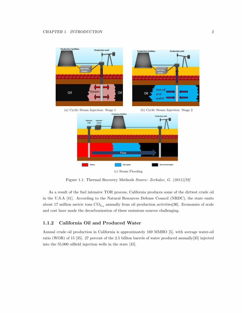
Thermal oil recovery (TOR) methods are enhanced oil recovery methods which do not alter the

pressure drive of the reservoir, but change fluid physical properties (e.g viscosity) to improve mobility.

TOR is commonly used to produce heavy oils (that is, crude oil with API gravity 20) e↵ectively,

with recovery factors up to 70 percent original oil-in-place (OOIP) [7]. TOR methods include Cyclic

Steam Injection (CSI), Steam Flooding, and Steam-Assisted Gravity Drainage (SAGD) [58].

1

CHAPTER 1. INTRODUCTION 2

(a) Cyclic Steam Injection: Stage 1 (b) Cyclic Steam Injection: Stage 2

(c) Steam Flooding

Figure 1.1: Thermal Recovery Methods Source: Zerkalov, G. (2015)[59]

As a result of the fuel intensive TOR process, California produces some of the dirtiest crude oil

in the U.S.A [41]. According to the Natural Resources Defense Council (NRDC), the state emits

about 17 million metric tons CO2eq annually from oil production activities[36]. Economies of scale

and cost have made the decarbonization of these emissions sources challenging.

1.1.2 California Oil and Produced Water

Annual crude oil production in California is approximately 169 MMBO [5], with average water-oil

ratio (WOR) of 15 [35]. 27 percent of the 2.5 billion barrels of water produced annually[35] injected

into the 55,000 oilfield injection wells in the state [45].


Figure 1.2: California Produced Water Allocation (2012) [55]

1.2 Statement of Problem

Carbon capture and sequestration (CCS) remains a leading option for carbon emissions mitigation

for point sources, which include oil and gas production facilities. Amine absorption is the most com-

mon commercial technology for post-combustion capture. However, the economics are prohibitive,

particularly for smaller, independent oil producers, and the high energy requirement for solvent

regeneration is a major driver for mitigation costs [20].

The abundance of disposed produced water presents a potential opportunity for a cheaper alter-

native to amine absorption for the mitigation of carbon dioxide emissions produced from thermal

oil recovery processes in local oilfields, given the fiscal incentives, such as those of the updated 45Q

Tax Credit[17] and the California Low Carbon Fuel Standard (LCFS).

1.3 An Opportunity for Cheap Capture?

The reformed 45Q Tax Credit incentivizes carbon capture projects across the United States, with

carbon pricing that ramps up to $35/ton for utilization projects, including CO2 EOR, and $50/ton

for geological storage projects, over 10 years [17]. The California Low Carbon Fuel Standard (LCFS)

is another fiscal incentive, which can be stacked with the 45Q credit. The reduction in the cost


barrier to mitigating emissions from the carbon intensive oil production process in the state, and

the potential for improved recovery and thus, higher revenues, could provide a means for sector

decarbonization.

This work examines the sizing and cost of traditional post-combustion capture equipment using

counter-current gas absorption required for decarbonizing oil production using oilfield produced

water, as well as benefits from marginal improved oil recovery from carbonated water injection, and

carbon capture federal tax credits. The focus of the study is a cost-benefit analysis of deploying this

capture project, and an examination of how outcomes vary with changes in key input like design

parameters, discount rates and marginal improved recovery revenue estimates.

While there is the absorption e�ciency challenge associated with using a solvent of limited solu-

bility for CO2 capture, which would require larger-sized equipment, as well as operational challenges

involved in pre-treatment, corrosion control and scale formation prevention, the question of the eco-

nomic viability of the technology remains, considering not only the tax incentives and the marginal

benefit of improved oil recovery as a result of carbonated water injection (CWI) into these water-

saturated oil reservoirs, but also cost performance when compared to the prevailing alternative

technology that is conventional capture using monoethanolamine solution. Unlike the conventional

system where an energy-intensive solvent regeneration system is required along with gas compression

and long-term gas plume monitoring due to significant leakage risk, CO2-laden water is injected into

the formation from which the water is produced, thus o↵ering formation pressure control, as well as

significantly reducing the risk of leakage, which could reasonably be expected to lower monitoring

costs and cost of capital.

1.4 Objectives

This thesis seeks to accomplish the following objectives, using the Pacific Coast Energy Company

(PCEC) LP. as a case study:

• design an absorption system for the capture CO2 from exhaust gas produced by oilfield steam

generators, using with an emissions output of 30,000 tons per annum in 2018.

• size a counter-current packed absorption column in a base case using chemical engineering

simulation tools and models, determining the minimum liquid loading and packed height re-

quirements for a base case design assumption at appropriate operating conditions.

• perform the aforementioned steps for choices of water and 30 weight percent MEA, the con-

ventional choice, as solvent.

• estimate capture project costs.


• conduct a cost-benefit analysis, assuming project qualifies for California Low Carbon Fuel

Standard credits, with marginal oil recovery improvement from carbonated water injection

(for the water system), and CO2-flooding (for the conventional system).

• test sensitivity of outcomes to changes in input of oil recovery benefit, discount rate, natural

gas and oil price forecasts, and qualifying captured emissions fraction, as is relevant to each

solvent choice scenario.

1.5 Limitations of Study

This study seeks to explore and compare the economic viability of two technology options for de-

carbonizing oil production processes which utilize thermal oil recovery, using PCEC as a case study.

In order to accurately assess returns on a specific investment option, detailed front end engineering

design, cost estimation, reservoir characterization, as well as injection and storage simulation studies

would need to be carried out for the PCEC Santa Maria basin formation, as in the case study, or

other specific storage site of interest.

Chapter 2

Literature Review

2.1 Introduction

California’s Global Warming Solutions Act of 2006 (AB32) and Executive Order S-3-05 set strict

standards for the emissions targets for the state, with a goal to lower greenhouse gas emissions to

150 MtCO2 eq/year, 80% below 1990 levels by 2050, while accommodating for both population and

economic growth[44]. Carbon capture and sequestration (CCS) is considered to be a key part of the

portfolio of technologies to achieve not only low carbon electricity generation, but also low carbon

fuel by 2020[44].

Oil production in California has declined at a rate of about 2% per year since 1990 due largely

in part to depleted oilfields in the San Joaquin Valley[13]. It is projected that this decline rate

will continue for at least another decade, subject to oil prices and technology in the oil and gas

industry[3].

Figure 2.1: California oil consumption (left) and production (right) since 1990. Source: U.S.Energy Information Administration[1], [2]

6

CHAPTER 2. LITERATURE REVIEW 7

However, the consumption of petroleum products has held steady in the state since 1990, as

shown in Figure 2.1. Thus, meeting the set emissions reductions target would require significant

reductions in carbon intensity on both demand and supply sides.

2.2 CO2 Capture With Produced Water and Brine

Carbon capture and sequestration (CCS) technology removes carbon dioxide (CO2) from point

sources which would otherwise emit the greenhouse gas into the atmosphere, or from air (as in Direct

Air Capture), and securely stores the CO2 in geologic formations. The most common method for

post-combustion capture of CO2 is counter-current gas absorption, in which a gas mixture containing

CO2, the solute gas, of a given concentration, is contacted with a liquid solvent which has a high

a�nity for the solute gas.

2.2.1 Produced Water Treatment

About 675 million barrels of produced water are injected into disposal wells annually in the state of

California [35]. Data on the geochemical properties of produced water is useful in establishing the

performance of the water as solvent for an absorption process. McMahom et al. (2018) [38] collect

geochemical and isotopic data for produced water from 22 oil wells across four oil fields in the San

Joaquin Valley of California.

The potential for utilizing this water is contingent upon the economic methods for produced water

treatment to process water quality. Treatment objectives include removing wax, grease, oil, organic

material, suspended solids, dissolved minerals, naturally occurring radioactive material (NORM),

and hardness which may either foul the process equipment or lower process e�ciency or both.

Arthur et al. (2005) [8] compare separation and operations performance of various water treatment

technologies, while Meng et al. (2016) [39] explored the feasibility of using oilfield produced water

to address water scarcity in the Central Valley of California, giving cost estimates based on a reverse

osmosis purification method.

2.2.2 Solubility of CO2 in Water

CO2 solubility characteristics in a given solvent significantly influences the rate and e�ciency of

separation from the gas phase. Low gas phase CO2 concentrations encountered in the e✏uent streams

from fossil fuel combustion in steam generators, and consequently, low liquid phase concentrations

of the solute gas, make Henry’s law appropriate for the dilute system[57]. Henry’s law for such a

component in the aqueous phase may be represented by equation (2.1)


fiw = xiwHi (2.1)

where fiw is the fugacity of component i in phase w, xiw is the mole fraction of i in w, and Hi

is the Henry’s law constant of component i.

Equation 2.1 is a single component definition of Henry’s law, and makes no assumptions about the

equilibrium state of the solution, and the obtained Henry’s law constant assumes a single component

gas phase. For a phase equilibrium to be achieved in a multicomponent system, equation 2.2 must

hold.

lnfjv = lnfjl = lnfjw (2.2)

for any phase m = l, v, w, and all components j = 1, 2, ...nc.

Thus, the fugacities of the solute gas, CO2, in the liquid and gas phases are equal at equilibrium.

If the gas phase is assumed to be a mixture of gas which exhibit ideal behavior, then the fugacity

of each pure gas component f⇤jat the temperature and pressure of the gas mixture, equals the total

gas system pressure P . The equilibrium distribution of a solute gas i between both phases may be

described in terms of the mole fraction of i in the aqueous phase xi, and the gas phase yi as in

equation 2.3.

xiwHi = yivP (2.3)

For ionic solvents, the solubility of a non-electrolyte solute in solution is significantly influenced

not only by temperature and pressure, but also by the natures of the non-electrolyte and electrolytes

in solution through a phenomenon called Setchenow’s ”salting-out”, originally proposed in 1892 [50].

Equation (2.7) relates the Henry’s law constant for CO2 in pure water, H0, to that in an electrolyte

solution, H.

log10

✓H

H0

◆= hI (2.4)

I =1

2

Xciz

2i

(2.5)

where I is the ionic strength of the solution in M, defined in equation (2.5), with ci being the


concentration of ions of species i, and zi being the charge on i. h in equation (2.7) is a quantity which

represents the sum of contributions of positive and negative ionic charges of dissociated species in

solution, with units of L/g [57]. This may be defined as in equation 2.6.

h = h+ + h� + hG (2.6)

Enick and Klara (1990) [23] determined that the solubility of CO2 in brine is a function of its

solubility in water and the percentage total dissolved solids (TDS) in the brine for pressures up to

85MPa, with no observed dependence on temperature or pressure. They prescribe the correlation

in equation 2.7 to correct for the e↵ect of TDS on CO2 solubility:

(2.7)wCO2, b = wCO2, w ⇥

⇣1.0� 4.893414⇥ 10�2 (TDS) + 0.1302838⇥ 10�2 (TDS)2

� 0.1871199⇥ 10�4 (TDS)3⌘

2.3 Carbonated Water Injection (CWI)

Carbon dioxide use for enhanced oil recovery (EOR) is a proven, well-established, commercial tech-

nology used in the oil and gas industry. Best practices for CO2 � EOR have the capacity to result

in a 5%-15% of original oil in place (OOIP) increase in oil production, depending on factors such as

reservoir petrophysical characteristics, fluid properties and depositional environment [25].

2.3.1 CWI vs CO2- and water-floods for improved oil recovery

The two main methods for CO2 flooding are miscible and immiscible flooding, and the class into

which a project falls depends on reservoir properties. At su�cient reservoir depth where pressure

is greater than the minimum miscibility pressure (MMP) for that reservoir, a miscible flood may

be possible. However, the overall performance of the CO2 flood is dependent on the geochemistry,

heterogeneity, porosity, permeability and permeability profile of the reservoir.

Generally, miscible floods are considered more e↵ective than non-miscible floods for EOR [9, 25],

although the incremental recovery achieved with miscible CO2 flooding is lower than industry expec-

tation of overall oil recovery, particularly with unconventional methods such as gravity stabilization

and double displacement recovery[40]. Factors such as low-e�ciency displacement and sweep, chan-

nel formation and early breakthrough reduce recovery[56]. For the purposes of carbon sequestration,

high sweep e�ciencies are desired for improved CO2 storage e�ciency.


Figure 2.2: Conventional CO2 flood (left) and CWI (right) Source: Esene et al. (2019)[24]

Sohrabi et al (2008)[52] show improved oil recovery with carbonated water injection in both cases

of secondary recovery, as well as in water saturated reservoirs for tertiary recovery, by up to 15%

OOIP. Martin (1951)[37] 12% improvement in oil recovery through CWI, while Lake et al. (1984)

reported up to 26% improvement in recovery due to CWI for tertiary EOR for light oil, and 2% of

pore volume for heavy oil. Johnson et al. (1952)[33] found recovery of 15%-25% with CWI over brine

flooding, with higher recovery at lower temperature due to increased CO2 solubility. Kilybay et al.

(2016)[34] compared recovery from coreflood experiments on secondary, tertiary and quarternary

recovery modes with seawater and seawater saturated with CO2, and found 5.7%-13.6% improved

recovery with carbonated seawater. Bisweswar et al. (2019) [11] review the prospects of CWI based

on current literature, with the key finding of up to 51% additional recovery of residual oil-in-place

at first injection, and 4% at second injection.

An additional benefit to carbonated water injection into reservoirs that have been water-flooded

is the ability for the carbonated water to mix with in-situ water, thereby reducing the e↵ects of

water shielding [47]. Unlike in conventional CO2 injection, at a certain temperature and pressure,

the quantity of CO2 injected into the reservoir at any time is solubility-limited, and displacement

e�ciency is controlled by the rate of mass transfer of gas between the oil and carbonated water

phases. There is therefore no separate, CO2-rich phase in the reservoir[21]. Since plume leakage

through cap-rock pores is a risk for carbon sequestration, one which limits the availability of suitable

reservoirs for carbon storage[31], carbonated water injection could allow for sequestration with lower

risk for gas leakage, and more available storage volume.


2.3.2 CWI sequestration projects

The Carbfix2[27] project showed fast-rate sequestration of captured acid gases, carbon dioxide and

hydrogen sulphide, from the exhaust of the Hellisheii geothermal power plant in Iceland, achieved

by mineralization in deep basaltic rocks. The geothermal gas from the plant, at 0.336 m/s, was rich

in acid gases, containing 63% CO2 and 21% H2S by volume. Capture was achieved by dissolution in

pure water at 200C and 6 bar in a scrubbing tower. The CO2 �H2S�laden water was injected at a

rate of 30-36kg/s, and mineralization of the carbon and sulphur was shown to occur within months

of injection, with costs coming to $25/ton of gas mixture sequestered.

Figure 2.3: Schematic of the scrubbing tower in the capture plant. The scrubbing tower is 12.5mhigh, 1m wide, and captures CO2 and other water-soluble gases with near-pure water injected at 6bar and 200C at the top. (Source: Gunnarsson et al.[27])

The original Carbfix project demonstrated the geologic solubility storage of 175tonnes of CO2

dissolved in 5000tonnes of water during injection in basalt formations[51]. The stream of near-pure

CO2 originated from a geothermal power-plant at Hellisheidi in Iceland. The largest risk of geologic

sequestration is leakage of gas into overlying fresh-water aquifers, or into the atmosphere, and the

injection of dissolved-phase CO2 significantly lowers this risk. In addition, more storage sites become

available for sequestration, since the need for a cap-rock seal is removed, and while sequestration

formations do not need to be as deep to ensure supercritical phase gas, more volume is required.

The carbon intensity of the Hellisheidi geothermal plant is about 21.6g CO2 per kWh, at contrast

with typical gas and coal power plants which range from 385g to 1000g CO2 per kWh. Since the gas

dissolution is an additional step to the capture and sequestration process, there is an added energy


penalty of 0.2% for the Hellisheidi, compared to 3%-10% for coal- and gas-fired power plants[51]. In

all cases, the bulk of cost is associated with the capture of CO2.

Burton and Bryant (2007)[14] determine the additional capital and operating costs to be paid as

the price of the aforementioned risk-reduction when additional facilities are used for CO2 dissolution

in brine, and compare these costs to those for conventional bulk-phase CO2 injection. For typical

power plants with capacities of 250-1000MW, capital costs increase by about 60%, with 3-9% increase

in energy consumption, and brine requirement on the order of millions of barrels per day, produced

from the target aquifer for injection.

Chapter 3

Methodology

3.1 Introduction

Oil and gas producers seeking to lower their carbon footprint are now incentivized by the updated

45Q and California Low Carbon Fuel Standard (LCFS) tax credits which can be claimed by the

operator of carbon capture facilities, provided they meet minimum requirements to generate these

credits[30]. One such producer in the state of California is the Pacific Coast Energy Company

(PCEC), which produces oil (and gas) from the Santa Maria basin at Orcutt Hill, and the Los

Angeles basin at West Pico, Sawtelle and East Coyote. At its Orcutt Hill facility, PCEC produces

30,000 tons of CO2 annually from the combustion of natural gas to fire steam generators used in the

thermal recovery of oil from the Orcutt Diatomite and Careaga formations. A cost-benefit analysis

of a potential capture facility with a capacity of 30 Mtons of CO2 is done, using PCEC as a case

study.

3.1.1 Produced water at PCEC Orcut Hill

The PCEC facility is located in the Santa Barbara county of California. About 6000 barrels of water

per day (bwpd) produced from the oilfield is treated, and used as feed to steam boilers for thermal

stimulation in the cyclic steaming process, while the rest is injected with 67 injection pumps through

58 waterflood injection wells into the Monterey, Point Sal and SX formations. Approximately 90,000

bwpd is injected. Figure 3.1 shows the layout of the water facility.

13

CHAPTER 3. METHODOLOGY 14

Figure 3.1: PCEC Water Schematic (Source: Pacific Coast Energy Company LP.)

3.1.2 Oil production at PCEC Orcutt Hill

According to the Annual Report filed with the Securities and Exchange Commission (SEC)[53] at

year-end 2018, PCEC produced an average of 2,500 barrels of oil equivalent per day (boe/day)

across its operations, with the 199 producing wells in the Santa Maria basin accounting for 67% of

gross producing wells in its portfolio. Of the 1,675 boe/day averaged in that year from our field of

interest, an average of 700 boe/day were produced from the Diatomite formation, 48 boe/day from

the Careaga formation, and the rest from its deep, conventional formations.

3.2 Analysis workflow

The workflow for the techno-economic analysis of the water-as-solvent capture project is summa-

rized in figure 3.2. Aspects of cost are estimated based on capital and annual fixed and variable

costs in raw cost scenarios, or using estimates from literature as the case may be, while benefits

include fiscal incentives in one scenario, and both fiscal and revenue incentives in another. Fiscal

incentives are derived from the California LCFS since the throughput of CO2 at PCEC is currently

too small to qualify for the 45Q credits, while revenue incentives include estimated marginal gains

from improvement in oil recovery from carbonated water injection.


Figure 3.2: Analysis workflow

3.3 Resource analysis

The exhaust gas from the steam generators is first analyzed. Fuel to the generators is natural gas

from two sources - gas produced from the PCEC Santa Maria field, and gas purchased from the

utility, SoCal Gas, in the volume ratio 2:1. The analysis of the fuel gas is shown in 3.3.

Combustion of this fuel gas mixture with 20% excess air produces exhaust gas with about 10mol%

CO2. The composition of cooled flue gas from the steam generators is approximated to insoluble

non-solute gas components (which is mainly nitrogen), and solute gas, CO2. The approximate

composition of the exhaust gas stream that feeds the capture facilities is shown in table 3.1.

Table 3.1: Exhaust gas composition

Component Molar Composition (%)

CO2 10.12

H2O 15.34

N2 70.86

O2 3.68


Figure 3.3: Steam Generator Fuel Gas Analysis

The availability of produced water resource governs CO2 solubility and capture rate limits, and

determines the necessity for alternate water source/ to achieve high capture rates. It is assumed that

the produced water is treated to a state consistent with specified total dissolved solids (TDS), and

ions in solution. The produced water pre-treatment and flue gas pre-cooling facilities are therefore


criticial to the process and considered within the scope of this study. Figure 3.4 shows the distribution

of injection rates in barrels of water per day (bwpd) for 56 injection wells in the oilfield.

Figure 3.4: Oilfield Produced Water Injection Rates

3.4 Capture system design

Equipment sizing is required to make capital and engineering cost estimates, as well as determine

operating limits. The commercial process simulator, Aspen Plus, is used to simulate the absorption

system and determine optimal converged specifications to achieve desired separation operations.

Two systems are studied and compared - water-based and conventional 30 wt% monoethanolamine

(MEA) capture systems.

3.4.1 Conventional capture system

The capture of CO2 is typically commercially done using an absorption process with alkanolamine-

water mixtures as solvent. Monoethanolamine (MEA), a primary amine with high heat of reaction

with CO2, is the most common industrial alkanolamine used for such capture processes as in the

Fluor (Economine FG Plus) process, as a 30 wt% mixture.

MEA is a primary amine with chemical formula NH2CH2CH2OH, which reacts in water to

form a weak base, with only 0.5% ionization to protonated ammonium form.

NH2CH2CH2OH +H2O ()+ NH3CH2CH2OH +OH� (3.1)

The absorption reaction of MEA with CO2 is rate-governed, with mechanisms involving the


formation of zwitterion species (RNH+2 COO�), and immediate neutralization by base to form

carbamate species (R2NCOO�).

CO2 +RNH2 () RNH+2 COO� (3.2)

RNH+2 COO� +B () RNHCOO� +BH+ (3.3)

where R is the alkanolamine functional group, CH2CH2OH, and B is either water H2O or base

RNH2 .

The formation of zwitterion dominates the rate of reaction, thus making the overall reaction

approximately first order with respect to MEA. The downside to the fast-reacting dynamics of MEA

with CO2 is the high energy requirement, and thus heating costs required to separate CO2 from the

solvent.

Di↵erent reaction mechanisms have been proposed for the formation of carbamate species; the

absorption/stripping model uses the reduced termolecular mechanism as depicted by equations 3.4

and 3.5.

2MEA+ CO2 () MEA+ +MEACOO� (3.4)

MEA+ CO2 +H2O () MEA+ +HCO�3 (3.5)


DCC

MEA capture system

CO2 injection

Flue gas from steam generator

Cooled flue gas

Captured CO2

Figure 3.5: MEA capture process flow block diagram

Figure 3.5 shows a simple block diagram which represents the conventional capture system flow.

The MEA capture process applied in this study is shown in Figure 2.

Hot flue gas from the steam generators, rich on CO2, is pre-cooled in a heat exchanger with

cold-side CO2-lean flue gas, before being cooled in a direct contact cooler (DCC), wherein some of

the entrained water vapor is removed as well. A fan is then used to blow the cooled flue gas into an

absorber. The schematic for the MEA system is shown in figure 3.6. Lean MEA solvent (ABSLEAN)

is fed to a countercurrent packed absorber (ABSORBER) along with cooled flue gas (GASIN). The

gas is fed at a rate of 0.2 kmol/s at 313K temperature and 1 atm. The CO2-rich solvent (ABSRICH)

is then heated, flashed to separate volatile gases, and pumped into a stripper column (REGEN) to

separate the CO2 from the bulk solvent phase in the equilibrium-governed reverse reaction flash

operation, recovering lean solvent (ABSLEAN) for re-use. The CO2 gas product is compressed for

storage in a subsurface reservoir.


Figure 3.6: MEA capture process schematic

The capture model is set up using the RADFRAC simulator, with the Electrolyte-NRTL thermo-

dynamic property basis model. First proposed by Chen et al. (1979, 1982) [15, 16], the Electrolyte-

NRTL, ’ELECNRTL’, has the capacity to handle a wide range of component concentrations in

aqueous solutions and mixed solvents. It models the excess Gibbs free energy of an electrolytic solu-

tion as a sum of energies from the contribution of both short-range, local ion-ion, molecule-molecule

or ion-molecule interactions, and long-range electrostatic ion-ion interactions.

Table 3.2: Absorber specifications

Specification Absober

Diameter 3mPacked height 6mPacking type Cascade Mini Rings (CMR), randomPacking size 44mmPacking material MetalVendor MTL

Stage calculations are made using a mixed flow model, wherein bulk properties for each phase

are taken to be the same as outlet properties for said phase from a specified stage. Heat and mass

balance calculations are done using a two-film assumption, with film discretization for accurate

modeling of the dynamics of the fast-rate concentration profile dynamics.

A 90% capture rate of CO2 is required for convergence, and the minimum solvent rate (Lmin)


for a given set of inputs converges when the energy supplied to the reboiler is su�cient to produce

a lean product stream with loading that matches the specified lean-loading. The required value

of Lmin varies with packed height, with less solvent needed with increasing contact surface area

available. If Lmin,1 is the minimum solvent rate required for an absorber with infinite packed

height, the typical chosen packed height would be that for which 20% excess Lmin,1 is required.

Figure 3.7 depicts a sensitivity study on Lmin and packed height, with the optimal packed height

determined to be 5.6 meters CMR at a lean-loading of 0.2 kmolCO2/kmolMEA. This optimal value

is not significantly changed at the specified diameter at higher lean-loading values, up to 6 meters

at 0.32 kmolCO2/kmolMEA.

0

500

1000

1500

2000

2500

3000

3500

4000

4500

5000

4 6 8 10 12 14 16 18 20 22 24 26 28 30 32 34 36 38 40 42 44 46 48 50 52 54 56 58 60 62 64 66 68 70 79 89 99 109 119 124 164 204 244 284 324 364 404 444 484 524 564 604

Lmin

(km

ol/h

r)

Packed height (m)

Lmin, opt

Figure 3.7: Optimal minimum solvent rate and packed height

Table 3.3 summarises the specifications for the absorber and stripper, including reboiler heating

duty, for 90% capture.

3.4.2 Water-based capture system

The proposed capture system which uses water comprises a much simpler process flow, wherein the

need for solvent regeneration is removed since captured CO2 is to be injected as carbonated water

as shown in figure 3.8. Hence, the main piece of equipment here is the packed absorber column,

with dimensions 2m diameter, 4m packed height, and 44mm metal CMR packings.


Table 3.3: Absorber and stripper specifications

Absorber Stripper Units

Top

Temperature 315.804 370.944 KDistillate rate 592.537 120.08 kmol/hrReflux rate 3,870.75 3,812.60 kmol/hrReflux ratio 6.5325 31.7505 dimensionless

Bottom

Temperature 327.809 378.562 KBottoms rate 3,836.11 3,782.84 kmol/hrBoil-up rate 658.187 83.2124 kmol/hrBoil-up ratio 0.17158 0.0212 dimensionlessHeat duty 0 2,023.33 kW

Figure 3.8: Water capture system block diagram

The CO2-water chemistry is equilibrium governed, with both Henry’s Law solubility and solvation

in aqueous solution playing roles in the overall thermodynamics and kinetics of the system.

CO2HCO2(==) CO2(g) (3.6)


CO2 +H2OK1() H2CO3 (3.7)

CO2 +OH� K2() HCO�3 (3.8)

H+ + CO2�3

K3() HCO�3 (3.9)

H+ +HCO�3

K4() H2CO3 (3.10)

H+ +OH� K5() H2O (3.11)

where HCO2 is the Henry’s Law constant, and Ki the equilibrium constant of each reaction i.

The ASPEN Plus model uses RADFRAC to simulate the capture of CO2 from cooled flue gas in

the packed absorber using purified produced water at 6 bar in an equilibrium-governed process. The

Electrolyte-NRTL thermodynamic model is also used here, with Henry’s Law for gas phase solubility

dynamics.

Due to the much lower solubility of solute gas, CO2, in the water solvent, the permissible system

capture rate is determined as a function of gas flow rate, varying from 144 kmol/hr to the upper

limit of 720 kmol/hr, given the total available water flow rate of 8.5 kmol/s.


0%

10%

20%

30%

40%

50%

60%

70%

80%

90%

100%

144161179196213230248265282300317334351369386403420438455472490507524541559576593611628645662680697714

Cap

ture

rate

Flue gas rate (kmol/hr)

Figure 3.9: Feasible capture rates with varying gas flow rate

The available water from the field achieves only 19.5% capture in a single pass. In order to

attain the desired 90% capture rate, the flue gas could be split into five trains of similarly-designed

absorbers, which would require an external source of water supply. The achievable capture rate for a

specified system does not improve with increased packed height, and higher system pressure results

in column flooding.

3.5 Cost estimation

A cost analysis for each system is done by estimating major cost aspects, including investment costs

for the major facilities, energy, consumables, flue gas cooling, water production, water purification,

and injection costs.


Table 3.4: Aspects of system costs

Aspect Conventional MEA Water

Flue gas cooling DCC DCC

Water production - Water wells

Water treatment - RO System

Heating Reboiler energy -

Injection CO2 flood CWI

Investment cost Absorber Absorber

Stripper

Heat exchanger

Heater

3.5.1 Investment Costs

The Inside Battery Limit (ISBL) project cost, assuming construction with stainless steel-lined casing

for the stripper and carbon steel for the absorber, and including installation and auxilliaries, is made

with the Peters and Timmerhaus (2003)[46] Chemical Engineering costing tool. The tool is based on

2002 US Dollars, with corrections made to 2018 US Dollars using the Chemical Engineering Plant

Cost Index (CEPCI) of both years (390.4 in 2002, 690.1 in 2018). Factored cost estimation is done

to determine the project cost at a 10% discount rate over 25 years in the base case. This discount

rate represents the internal rate PCEC uses in reporting its revenue to the SEC (as of year-end

2018).

Table 3.5 summarizes cost factors used in the cost analysis for the capture project. It is assumed

that current labor availability at the site satisfies sta�ng requirements are su�cient to cover the

new project.


Table 3.5: Capital cost factors

Parts and spares 0.15 EC

Engineering + installation 0.2 EC

Outside Battery Limit 0.2 EC

Contigency 0.1 EC

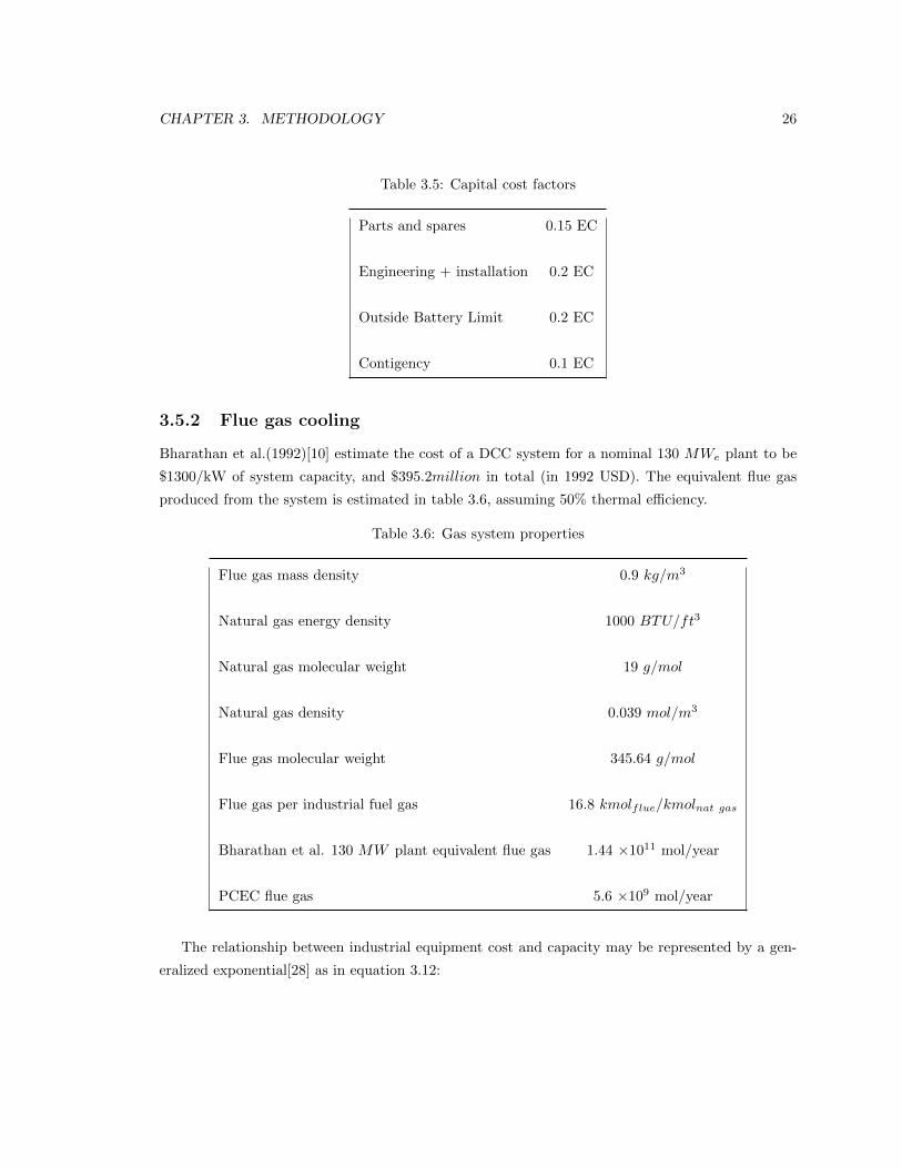
3.5.2 Flue gas cooling

Bharathan et al.(1992)[10] estimate the cost of a DCC system for a nominal 130 MWe plant to be

$1300/kW of system capacity, and $395.2million in total (in 1992 USD). The equivalent flue gas

produced from the system is estimated in table 3.6, assuming 50% thermal e�ciency.

Table 3.6: Gas system properties

Flue gas mass density 0.9 kg/m3

Natural gas energy density 1000 BTU/ft3

Natural gas molecular weight 19 g/mol

Natural gas density 0.039 mol/m3

Flue gas molecular weight 345.64 g/mol

Flue gas per industrial fuel gas 16.8 kmolflue/kmolnat gas

Bharathan et al. 130 MW plant equivalent flue gas 1.44 ⇥1011 mol/year

PCEC flue gas 5.6 ⇥109 mol/year

The relationship between industrial equipment cost and capacity may be represented by a gen-

eralized exponential[28] as in equation 3.12:


C = aXb (3.12)

where C represents cost, X the capacity or throughput, a, a system constant, and b, a scale

coe�cient which factors in economies (or diseconomies, depending on whether returns are increasing

or decreasing with scale). The scale factor for typical industrial equipment varies, with a mean value

taken to be b = 0.6[28]. With C = $395.2m, the system constant is found to be a = 79.7$/(mol)0.6.

Learning rates for power plant equipment in literature are up to 30%[48], and capacity having

increased by 3.4 times since 1992[6], costs are assumed to have reduced 50%. A summary of the

calculated cost of DCC is presented in table 3.7.

Table 3.7: Unit DCC cost estimate

1992 million USD 2018 million USD

Haldi and Whitcomb[28] system 392.5 351.4

PCEC system 56.3 50.4

3.5.3 Water Production

As demonstrated by the Aspen water model, significant additional quantities of water would be

required for capture. Assuming adequate brine disposal wells already exist on the PCEC site, water

production wells su�cient to produce an additional 340,000 bwpd would need to be drilled. For

typical commercial wells which produce 500 gpm [26, 29], with each well assumed to cost $32, 500

each (including tanks, pumps, poles, etc), a total of 20 wells would be required to meet the resource

requirement for the capture project.

3.5.4 Water Treatment

Meng et al. (2016)[39] estimate the cost of treating produced water in Central Valley, California,

using a reverse osmosis process, to address scarcity needs in the region. The average annualized

estimate was $0.20/m3 water in 2018 USD. This value is used in calculating water treatment cost

for the water-based capture system, with an additional 20% cost factor for corrosion inhibition.

3.5.5 Injection

In the conventional system, the captured CO2 gas goes through multi-stage dehydration and com-

pression before transport to depleted oil and gas fields (DOGF) for storage. Figure 3.10 shows the


cost-breakdown of storage costs, with these costs excluding transport of the gas, for legacy and

non-legacy wells in both DOGF and saline aquifer (SA) fields.

Rubin et al. (2015)[49] studied various quoted transport and storage costs from literature, with

numbers from the IPCC for short distance transport over 250 km estimated, in 2018 USD, to be

$6.20/ton CO2. Thus, transport and storage costs for sequestration in onshore DOGF wells, in

total, averages $12/ton CO2.

0.4 0.4

2.6

0.2 0.3

7.0

0.4

1.5

1.2

0.9

5.2

3.7

0.7

0.7

0.7

2.6

2.6

3.1

1.3

1.3

0.7 2.1

2.1

0.8

1.2

1.2

1.2

1.3

1.3

1.3

Onshore DOGF Legacy Onshore DOGF Non-legacy

Onshore Saline aquiferNon-legacy

Onshore Saline aquiferLegacy

Offshore DOGF Non-legacy

Offshore DOGF Legacy

Close Down

MMV

Operating

Injection Wells

Structure

Pre FID

3.9

5.1

6.4

7.3

11.7

16.9

Close down

Operating

MMV

Injection wells

Structure

Pre FID

Decommisioning and liability transfer

OPEX, new observation wells, post-closure monitoring, final seismic survey

Operations and maintenance

New and re-used injection wells, legacy well remediation

Platform new/re-use

Modeling/logging costs, seismic survey, injection testing, new exploration wells, permitting

Figure 3.10: Aspects of CO2 storage costs

Unit cost estimates for carbonated water injection and monitoring were assumed using the Carb-

Fix2 project as a proxy, which injected 0.173 kg/s CO2 and 0.10 kg/s H2S[27]. Assuming no new

well drilling is required, and adjusting for gas density and solubility by mass ratio, injected costs are

estimated to be $3.80/ton CO2 (in 2018 USD).

3.5.6 Operating and other recurring costs

For the conventional MEA system, a significant variable cost is the cost of heating supplied to the

reboiler. It is assumed that natural gas is fired to supply energy required for solvent recovery with


the generation of steam at 60% e�ciency. Figure3.11 shows the EIA energy outlook delivered natural

gas price forecast in 2018 USD.

$0

$1

$2

$3

$4

$5

$6

2019

2020

2021

2022

2023

2024

2025

2026

2027

2028

2029

2030

2031

2032

2033

2034

2035

2036

2037

2038

2039

2040

2041

2042

2043

2044

2045

2046

2047

2048

2049

2050

Del

ieve

red

gas

pric

e ($

/GJ)

Year

Figure 3.11: EIA Energy Outlook delivered natural gas price forecast

Additionally, the amine solvent used is subject to both oxidative and thermal losses to the order

of 1.5 kgMEA/tonCO2 [43]. The lost solvent is assumed to be replaced annually as consumables, along

with corrosion inhibitor, which is assumed to cost 20% of the MEA sorbent[54]. Other annual fixed

costs and working capital are estimated using cost factors summarized in table 3.8.


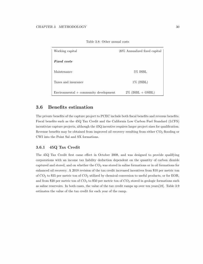
Table 3.8: Other annual costs

Working capital 20% Annualized fixed capital

Fixed costs

Maintenance 5% ISBL

Taxes and insurance 1% (ISBL)

Environmental + community development 2% (ISBL + OSBL)

3.6 Benefits estimation

The private benefits of the capture project to PCEC include both fiscal benefits and revenue benefits.

Fiscal benefits such as the 45Q Tax Credit and the California Low Carbon Fuel Standard (LCFS)

incentivize capture projects, although the 45Q incentive requires larger project sizes for qualification.

Revenue benefits may be obtained from improved oil recovery resulting from either CO2 flooding or

CWI into the Point Sal and SX formations.

3.6.1 45Q Tax Credit

The 45Q Tax Credit first came e↵ect in October 2008, and was designed to provide qualifying

corporations with an income tax liability deduction dependent on the quantity of carbon dioxide

captured and stored, and on whether the CO2 was stored in saline formations or in oil formations for

enhanced oil recovery. A 2018 revision of the tax credit increased incentives from $10 per metric ton

of CO2 to $35 per metric ton of CO2 utilized by chemical conversion to useful products, or for EOR,

and from $20 per metric ton of CO2 to $50 per metric ton of CO2 stored in geologic formations such

as saline reservoirs. In both cases, the value of the tax credit ramps up over ten years[18]. Table 3.9

estimates the value of the tax credit for each year of the ramp.


Table 3.9: 45Q Tax Credit Value Ramp (Source: Clean Air Task Force (2019) [42])

CalendarYearBeginningIn

EOR(Nominal$pertonneofCO2)

Saline(Nominal$pertonneofCO2)

2017 $12.83 $22.662018 $15.29 $25.702019 $17.76 $28.742020 $20.22 $31.772021 $22.68 $34.812022 $25.15 $37.852023 $27.61 $40.892024 $30.07 $43.922025 $32.54 $46.962026 $35.00 $50.00

From the year 2027 onward, the incentive is received a $35 per tonne CO2 stored for projects

which are still within term. Qualifying projects which begin construction prior to January 1, 2024

may claim the tax credit for up to 12 years after commencing service. There is a 100,000 tonnes

CO2 per year minimum for EOR projects, and 25,000 tonnes CO2 per year minimum for non-EOR

projects[17].

3.6.2 California Low Carbon Fuel Standard

The California Low Carbon Fuel Standard is a measure, established under the California Global

Warming Solutions Act of 2006 (AB32), to reduce the greenhouse gas (GHG) emissions intensity of

the transportation fuel pool in the state, adopted by the California Air Resources Board (CARB).

Recents amendments limit the price of LCFS credit transfers to the Credit Clearing Market (CCM)

price cap of $200/tonCO2eq in 2016 USD, equivalent to $209.35 2018 USD used as reference here[32].

Figure 3.12 shows the trend of LCFS prices, which has climbed mostly, besides a brief dip in 2017,

and reached a peak of $217 early in 2020.


Figure 3.12: LCFS Price trend

Clearly defined system boundaries must be established for qualifying capture projects, with

combustion, embedded, land use, vented, leaked, and fugitive emissions deducted from the proven

metered injected quantity of GHGs, which could include not only CO2, but also equivalent warming

quantities of CO, CH4, N2O, and volatile organic compounds (VOCs)[12]. In addition, between

8%-15% of credits are deposited as a bu↵er, in case of leakage. Thus, only a fraction of captured

emissions qualifies to receive the LCFS credits.

For EOR projects, recycled CO2 from produced water or associated gas would ideally be de-

ducted, but in the case of PCEC, the associated gas, containing recycled CO2 is used in firing the

steam generator, and thus retained within the system boundary.


(a) System boundary for sequestration in depleted oil and gas reservoirs or saline aquifers

(b) System boundary for CO2-EOR project

Figure 3.13: System boundary for LCFS-qualifying CCS project, Source: California Air ResourcesBoard (2018)[12]


3.6.3 Carbonated Water Injection and CO2 Flooding for Enhanced Oil

Recovery

According to the year-end 2018 Annual Report filed by the Pacific Oil Trust with the SEC, average

daily production of crude oil across all wells in both the Santa Maria and Los Angeles basins was 2,500

boe/day. 67% of 299 total production wells drain from the Santa Maria basin, for an average basin

production of 1,675 boe/day. The Orcutt Diatomite formation produced about 700 boe/day, while

Careaga produced approximately 48 boe/day. Thus, average production from the Monterey/Point

Sal formations, into which produced water is injected for waterflooding for EOR, was 927 boe/day,

or 0.34 MMboe/year.

In the base case scenario, an improvement in recovery is taken to be 5%, with the assumption that

this improvement in oil recovery translates to a constant improvement in oil production, starting

one year after the commencement of CWI. For the case of CO2 flood, possible improved recovery in

OOIP could be as high as 40%. The revenue from the sale of this crude oil constitutes a secondary

benefit to PCEC. A forecast of oil prices is used to estimate the expected value of this revenue

increase. Figure 3.14 shows the Energy Information Agency (EIA) price forecast Brent Crude Oil

to the year 2050 in both 2019 US Dollars, future values at a 3% discount rate, and the equivalent

2018 US Dollar values at the December 2019 real interest rate of 2.25%.

Figure 3.14: Crude Oil price forecast


3.7 Sensitivity Analyses

The solubility dynamics and subsequent sizing of the absorption equipment, is strongly dependent

on the design and operating conditions of the absorber. It is therefore important to see how changes

over a range of feasible capital costs, as well as anticipated cost of capital, project life, capture rate,

and additional improved oil recovery would impact the net present value of benefits from the project

investment.

Table 3.10 lists the parameters to which the sensitivity of net benefits from both the CWI and

MEA-based CO2-flood capture projects are tested, as well as the input bounds of these parameters

used.

Table 3.10: Sensitivity analysis input parameters

Input parameter Unit Base Case Lower Bound Upper Bound

Discount rate % 10 5 30

EOR Improvement % 5 0 40

Natural gas price forecast variation % 0 -50 50

Oil price forecast variation % 0 -50 50

Initial capital investment requirement variation % 0 -50 50

Unit water treatment cost factor variation % 0 -50 50

Qualifying fraction of captured CO2 % 50 10 90

Chapter 4

Results and Discussion

4.1 Introduction

The results for system costs are discussed for both the proposed CWI and conventional capture

PCEC projects. For all scenarios, it is assumed that 90% of CO2 gas produced on the field is

captured. In the case of the proposed CWI project, the available produced water resource has, as

described in the previous chapter, been determined to be insu�cient to achieve this capture goal,

thus necessitating water production infrastructure, the cost for which is factored into project costs.

It is assumed that only one-fifth of the produced water resource used in the process is sourced from

available water on the field, which would otherwise have been injected. Additional water production

facilities are therefore required, which incur additional costs in the CWI project. The net present

value of net benefits are also assuming both fiscal and revenue benefits from improved oil recovery.

Sensitivity analyses are then performed to determine how variation in input listed in table 3.10 a↵ect

the NPV net benefit from each proposed project.

4.2 Cost analysis

Table 4.1 summarizes required investment cost for equipment, which is assumed to include the cost

of installation, engineering and auxilliaries. The cost of the direct-contact cooler (DCC) unit is

estimated separately, at $56.4 million. A one-time solvent cost of $1.5 million is incurred, with lost

solvent replenished annually. These costs are annualized, and in addition to annual solvent, natural

gas heating, and CO2 injection costs, constitute annual project costs.

36

CHAPTER 4. RESULTS AND DISCUSSION 37

Table 4.1: MEA system equipment capital cost

Equipment Cost (2018 USD)

Absorber $167,603.80

Stripper $373,587.33

Reboiler $521,548.73

Heat recovery heat exchanger $73,777.42

The net present value of costs for the MEA project over its 25-year life is $42.28 million, with

the bulk of those costs associated with fuel for solvent regeneration in the reboiler, flue gas cooling,

and CO2 compression, transport and storage, as shown in figure 4.1.

Lower vendor-quoted DCC unit costs could significantly impact both the distribution of cost

contributions and the project net present value cost.

Heating32%

Injection22%

Fixed O&M5%

Fixed capital (excluding DCC unit)…

DCC31%

Solvent/Consumables9%

Figure 4.1: Breakdown of annualized costs for proposed MEA project


For the CWI project, it is assumed that five trains of absorption equipment, each consisting

majorly of a packed absorber, are used, with each costing $263,000. In this case, the NPV system

cost over the 25-year project life is $67.67 million, with the majority of costs incurred by the reverse-

osmosis water treatment process, which is essential in removing entrained hydrocarbons and dissolved

minerals from water, which may salt-out potentially soluble CO2 gas and form scale that damage

process equipment. The distribution of cost factors in the proposed CWI project is shown in figure

4.2.

Water Treatment87.92%

Injection1.83%

Fixed O&M1.70%

Fixed capital (excluding DCC unit)…

DCC8.22%

Water Production0.11%

Figure 4.2: Breakdown of annualized costs for proposed CWI project

4.3 Benefits analysis

Currently, emitted equivalent CO2 emissions from the PCEC facility are penalized on the carbon

market at the prevailing carbon price. Projections for this carbon price, as presented in Table 3.9

dictate the magnitude of emissions penalties avoided by capturing 90% of the CO2 produced from

oil production operations.

In addition, it is assumed in the base case that only 50% of the captured emissions qualify for the

LCFS, after leak bu↵er, fuel combustion, vented, and embedded equivalent CO2 emissions are all


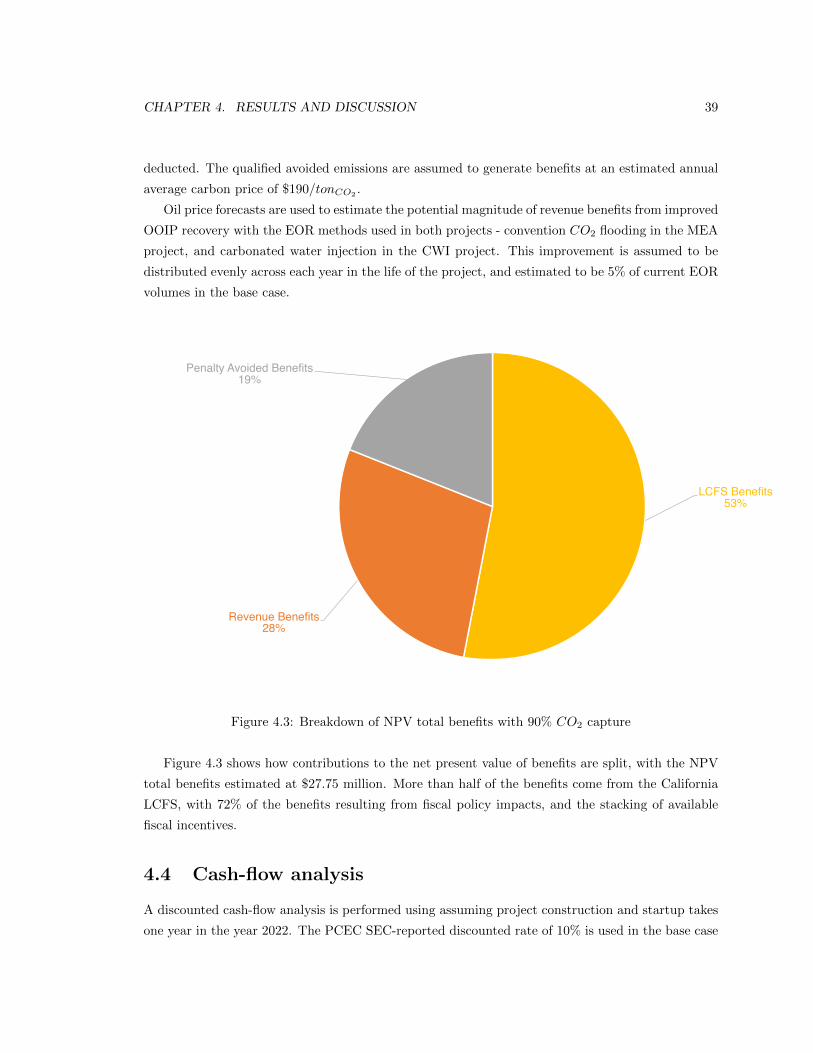
deducted. The qualified avoided emissions are assumed to generate benefits at an estimated annual

average carbon price of $190/tonCO2 .

Oil price forecasts are used to estimate the potential magnitude of revenue benefits from improved

OOIP recovery with the EOR methods used in both projects - convention CO2 flooding in the MEA

project, and carbonated water injection in the CWI project. This improvement is assumed to be

distributed evenly across each year in the life of the project, and estimated to be 5% of current EOR

volumes in the base case.

LCFS Benefits53%

Revenue Benefits28%

Penalty Avoided Benefits19%

Figure 4.3: Breakdown of NPV total benefits with 90% CO2 capture

Figure 4.3 shows how contributions to the net present value of benefits are split, with the NPV

total benefits estimated at $27.75 million. More than half of the benefits come from the California

LCFS, with 72% of the benefits resulting from fiscal policy impacts, and the stacking of available

fiscal incentives.

4.4 Cash-flow analysis

A discounted cash-flow analysis is performed using assuming project construction and startup takes

one year in the year 2022. The PCEC SEC-reported discounted rate of 10% is used in the base case


for both proposed projects, with 2018 as the base year for discounting. The bulk of the upfront

capital requirement for both projects come from the DCC unit payment.

For the MEA project, about 40% of costs are incurred upfront in Year 0 (2022), while annual total

benefits exceed annual costs from operations and maintenance, injection, consumables and heating

fuel. Figure 4.4 shows the discounted cash-flow diagram for the MEA project, with breakeven never

being reached in the base case within the 25-year life of the project. The NPV net benefit of this

project is estimated at ($14.53 million).

Figure 4.4: MEA project discounted cash-flow diagram

The CWI project requires a similar net present value upfront capital investment. However,

estimated annual costs are larger than those for the MEA project, with water treatment costs

dominating. These annual costs in the base case exceed annual benefits, thus resulting in a negatively

trending net cash-flow, as depicted in figure 4.5. The NPV net benefit of the proposed CWI project


is estimated at ($39.93 million).

Figure 4.5: CWI project discounted cash-flow diagram

4.5 Sensitivity analyses

The variations of project net present value net benefit with changes in input such as discount rate,

oil price, EOR improvement, capital cost, qualifying emissions fractions and annual variable costs

like water treatment and natural gas fuel, are explored. The ranges over which inputs are varied are

summarized in Table 3.10.

For the proposed CWI project, annual water treatment costs represent the bulk of project costs.

Therefore, higher discount rates penalize these future amounts more the farther in time they occur,

in net present terms, thus favoring the NPV project net benefit valuation. In the case of the proposed


MEA project, upfront capital costs perform better on the cash-flow sheet at lower discount rates

than that used in the base case. As discount rates are increased however, the NPV MEA project

net benefit only worsens slightly, as poorer performance of large upfront capital cost is tempered

by recurring annual variable cost e↵ect on cash-flow. At the discount rate increases to 20%, an

inflection is noticed (see figure 4.6), as the e↵ects of the higher discount rate on recurring annual

costs of injection and heating natural gas fuel, outweigh those on upfront capital payment.

-200%

-100%

0%

100%

200%

300%

400%

500%

-100%-50%-39%-29%-20%-10% 0% 10

%20%30%40%60%90%120%150%180%220%280%340%400%460%510%560%620%680%

% C

han

ge

in N

PV

net

ben

efit

s

% Change in input

Discount rate EOR improvementAverage oil price Capital costAverage natural gas price Qualifying avoided emissions fractionNPV = 0

Figure 4.6: MEA project sensitivity analysis

Both projects show only mild linear sensitivity to average annual oil and natural gas price vari-

ations, while the impact of upswings in average oil prices and proved qualifying emissions fractions

on NPV net benefit breakeven (that is, at NPV = 0), is more significant in the MEA project.


Variation in capital cost estimates, which include the cost of DCC units, significantly impact

project cost performance, more so in the case of the proposed MEA project. If the required capital

investment reduces by 40% for the MEA project, investment breakeven is achieved, all things being

equal, while a 50% reduction in capital cost, which would yield $3.38 million in NPV net benefits

with the MEA project, only achieves a 50% improvement in NPV net benefits for the water project,

with a value of ($21.9 million), as shown in figure 4.7 below.

-100%

-50%

0%

50%

100%

150%

-100%-60%-45%-39%-30%-24%-20%-13% -8% 0% 8% 13

%20%29%34%40%50%70%90%110%130%150%170%190%220%260%300%340%380%420%460%500%520%560%600%640%680%

% C

han

ge

in N

PV

net

ben

efit

s

% Change in input

Discount rate EOR improvementAverage oil price Capital costWater treatment cost Qualifying avoided emissions fractionNPV = 0

Figure 4.7: CWI project sensitivity analysis

For both projects, the NPV net benefit valuation is most sensitive to the estimated OOIP im-

proved recovery with the designated EOR methods. A marginal EOR improvement of 30% would

be required for CWI project to breakeven, all things being equal. This value would be in the range


of optimistic expectations from a carbonated water injection EOR project. However, only a 15%

marginal EOR improvement would achieve breakeven with the proposed MEA project, a value well

within the range of expectations for such a recovery project.

Chapter 5

Conclusions

While neither proposed project yields positive net benefit in the base scenario explored, the MEA

project appears to show more promise, in terms of NPV net benefit valuation breakeven. Positive

variation in a combination of inputs, such as lower capital costs, cheaper DCC unit estimates, higher

proven LCFS qualifying fraction and higher EOR improvement, would improve the MEA project

investment benefits outlook.

The actual provable estimates for LCFS qualifying captured emissions fractions would di↵er

between the conventional MEA and CWI projects, since the technology utilized in the CWI project

reduces the likelihood of leakage, both from surface facilities which process dissolved phase CO2,

and from injection formations in storage. However, the demonstrable EOR improvement that may

be obtained from the conventional MEA project may or may not be much more significant than

that from the CWI project. The injection of pure stream of supercritical CO2 may result in better

recovery, but the formation of channels and fingering e↵ects may limit reservoir sweep with the CO2

flood. Thus, core flood experiments and reservoir simulations would be required to address these

important sources of uncertainty for both proposed projects.

In the case of the proposed MEA project, upfront capital costs perform better on the cash-

flow sheet at lower discount rates, which may justify consideration for investment given the current

market performance and slash in national interest rates. However, if significant cost reductions in

water treatment were available, the proposed CWI project would be competitive.

In addition to reservoir characterization and simulation study to quantify provable qualifying

emissions, more detailed front-end engineering design and cost estimation based on equipment ven-

dor quotes would give firm distributions of expected costs and benefits. These may be used for

further study into uncertainty quantification, such as Monte Carlo simulations, to determine both

the expected value of project NPV net benefits, and the probability distribution of the net benefits

over the life of the project under uncertainty.

It is worthy of note that there is a unique advantage to the CWI project over the MEA project

45

CHAPTER 5. CONCLUSIONS 46

that is di�cult to quantify - the associated leakage risk reduction with the injection of dissolved

phase CO2, whereby the timelines for solubility and mineral trapping may be expedited, as well as

reservoir pressure and injection front expanse better controlled. However, there are yet concerns

around water consideration, one of which is the pressure build up in the reservoir caused by the

injection of water. Simulation study into the magnitude of pressure buildup would be required,

as well as reservoir pressure management operations. Environmental impact concerns also exist,

particularly given the climate of the state of California, and recent experiences of drought.

An alternative project consideration which could combine unique merits from both presented

MEA and water systems would be one where in surface capture facilities utilize MEA in a con-

ventional process, producing a high-purity stream of CO2 gas which may then be dissolved in the

produced water within the well-bore at high pressure, and summarily injected. This would merge the

more favorable economics of the MEA project with the storage leak risk-reduction obtained from

carbonated water injection, while removing the high-cost penalty of water production and water

treatment required for surface water capture processing.

Bibliography

[1] U.S Energy Information Administration. Crude oil production.

https://www.eia.gov/dnav/pet/pet˙crd˙crpdn˙adc˙mbbl˙a.htm, 2017.

[2] U.S Energy Information Administration. State energy data system. https://www.eia.

gov/state/seds/, 2017.

[3] U.S Energy Information Administration. Annual energy outlook 2018. http://www.eia.

gov/forecasts/aeo/, 2018.

[4] U.S Energy Information Administration. California: State profile and energy estimates.

https://www.eia.gov/state/analysis.php?sid=CA, 2018.

[5] U.S Energy Information Administration. Petroleum and other liquids: California field produc-

tion of crude oil. https://www.eia.gov/dnav/pet/hist/LeafHandler.ashx?n=pets=mcrfpca1f=a,

2019.

[6] U.S Energy Information Administration. Electricity explained: Electricity generation, capacity,

and sales in the united states. https://www.eia.gov/energyexplained/electricity/electricity-in-

the-us-generation-capacity-and-sales.php, 2020.

[7] J. Alvarez. and S. Han. Current overview of cyclic steam injection process. Journal of Petroleum

Science Research, 2:116–127, 2013.

[8] J.D. Arthur, B.G. Langhus, and C. Patel. Technical summary of oil gas produced water

treatment technologies. Technical report, ALL Consulting, LLC, 2005.

[9] K. Asghari and F. Torabi. E↵ect of miscible and immiscible co2 injection on gravity drainage:

Experimental and simulation results. SPE Symposium on Improved Oil Recovery, 20-23 April,

Tulsa, Oklahoma, USA. Society of Petroleum Engineers.

[10] Desikan Bharathan, Edward Hoo, and Paul D’Errico. An assessment of the use of direct contact

condensers with wet cooling systems for utility steam power plants. Technical report, National

Renewable Energy Lab., Golden, CO (United States), 1992.

47

BIBLIOGRAPHY 48

[11] G. Bisweswar, A. Al-Hamairi, and S. Jin. Carbonated water injection: an e�cient eor approach.

a review of fundamentals and prospects. https://doi.org/10.1007/s13202-019-0738-2, 2019.

[12] California Air Resources Board. Carbon capture and sequestration protocol un-

der the low carbon fuel standard. https://ww2.arb.ca.gov/sites/default/files/2020-

03/CCS˙Protocol˙Under˙LCFS˙8-13-18˙ada.pdf, 2018.

[13] A.R. Brandt. Oil depletion and the energy e�ciency of oil production: The case of california.

sustainability. Sustainability, 3(12). 1833–54. DOI:10.3390/su3101833, 2011.

[14] M Burton and S Bryant. Eliminating buoyant migration of sequestered co2 through surface

dissolution: implementation costs and technical challenges, spe 110650, proceedings, 2007 spe

ann. In Tech. Conf. Exhib., Anaheim, CA, pages 11–14, 2007.

[15] Ch Chen. Ch., britt, hi, boston, jf, evans, lb” extension and application of the pitzer equation

for vapor-liquid equilibrium of aqueous electrolyte systems with molecular solutes.”. AIChE

Journal, 25(5):820–831, 1979.

[16] Chau-Chyun Chen, Herbert I Britt, JF Boston, and LB Evans. Local composition model for

excess gibbs energy of electrolyte systems. part i: Single solvent, single completely dissociated

electrolyte systems. AIChE Journal, 28(4):588–596, 1982.

[17] J. Christensen. Primer: Section 45Q tax credit for carbon capture projects.

https://www.betterenergy.org/blog/primer-section-45q-tax-credit-for-carbon-capture-

projects/, 2019.

[18] Title 26 United States Internal Revenue Code. 26 usc 45q: Credit for carbon oxide sequestration.

https://uscode.house.gov/view.xhtml?req=(title:26%20section:45Q%20edition:prelim), 2018.

[19] M.J. Coren. California’s 2018 legislative blitzkrieg delivered its most ambitious climate

policies ever. https://qz.com/1409065/californias-2018-legislative-blitzkrieg-delivered-its-most-

ambitious-climate-policies-ever/, 2018.

[20] J. David and H. Herzog. The cost of carbon capture. Technical report, Massachusetts Institute

of Technology (MIT), Cambridge, MA, USA, 2015.

[21] Y. Dong, B. Dindoruk, C. Ishizawa, and E.J. Lewis. An experimental investigation of carbonated

water flooding. SPE-145380, 2011.

[22] H.M. El-Houjeiri, M.S. Masnadi, K. Vafi, J. Du↵y, and A.R. Brandt. Oil production greenhouse

gas emissions estimator opgee v2.0b user guide technical documentation. Technical report,

Stanford University, 2017.

BIBLIOGRAPHY 49

[23] R.M. Enick and S.M. Klara. Co˙2 solubility in water and brine under reservoir conditions.

https://doi.org/10.1080/0098644900890574, 1990.

[24] Cleverson Esene, Nima Rezaei, Amer Aborig, and Sohrab Zendehboudi. Comprehensive review

of carbonated water injection for enhanced oil recovery. Fuel, 237:1086–1107, 2019.

[25] P. Gao and B. Towler. Integrated investigation of enhanced oil recovery in south slattery min-

nelusa reservoir, part 2: Co2 miscible injection. Petroleum Science and Technology, 30(24):2543–

2551, 2012.

[26] Home Guide. How much does it cost to drill or dig a well? https://homeguide.com/costs/well-

drilling-cost, 2019.

[27] Ingvi Gunnarsson, Edda S Aradottir, Eric H Oelkers, Deirdre E Clark, Magnus or Arnar-

son, Bergur Sigfusson, Sandra O Snæbjornsdottir, Juerg M Matter, Martin Stute, Bjarni M

Julıusson, et al. The rapid and cost-e↵ective capture and subsurface mineral storage of carbon

and sulfur at the carbfix2 site. International Journal of Greenhouse Gas Control, 79:117–126,

2018.

[28] John Haldi and David Whitcomb. Economies of scale in industrial plants. Journal of Political

Economy, 75(4, Part 1):373–385, 1967.

[29] Thomas Harter. Water well design and construction. UCANR Publications, 2003.

[30] I Havercroft and A Townsend. The lcfs and ccs protocol: An overview for policymakers and

project developers, 2019.

[31] H.J. Herzog. The economics of co˜ 2 separation and capture. Technology-Elmsford-Journal of

the Franklin Institute, Journal of Science Serving Legislative Regulatory and Judicial Systems,

7:13–24, 2000.

[32] Abbey Hudson, Dione Garlick, and Caroline Monroy. Calif. low carbon fuel standard price cap

is a trade-o↵. https://www.gibsondunn.com/wp-content/uploads/2020/02/Hudson-Garlick-

Monroy-Calif.-Low-Carbon-Fuel-Standard-Price-Cap-Is-A-Trade-O↵-Law360-02-07-2020.pdf,

2020.

[33] W. Johnson, R. Macfarlane, J. Breston, and D. Neil. Laboratory experiments with carbonated

water and liquid carbon dioxide as oil recovery agents. Producers Monthly, 17, 1952.

[34] A. Kilybay, G. Bisweswar, N.C. Thomas, and P. Aras. Hybrid eor technology: carbonated water

and smart water improved recovery in oil wet carbonate formation. SPE-182567, 2016.

[35] K. LaFond. Infographic: Wastewater in california’s oil fields. Circle of Blue Water News, 2015.

BIBLIOGRAPHY 50

[36] K. Law, M. Chan, and S. Mui. Carbon reduction opportunities in the california petroleum

industry. Technical report, 2013.

[37] J.W. Martin. Additional oil production through flooding with carbonated water. Producers

Monthly, 15(7):18–22, 1951.

[38] P.B. McMahon, J.T. Kulongoski, A. Vengosh, A.V. Cozzarelli, M.K. Landon, Y.K. Kharaka,

J.M. Gillespie, and T.A. Davis. Regonal patterns in geochemistry of oil-field water, southern san

joaquin valley, california, usa. Applied Geochemistry, Volume 98, November 28, Pages 127-140,

2018.

[39] M. Meng, M. Chen, and K.T. Sanders. Evaluating the feasibility of using produced water from

oil and natural gas production to address water scarcity in california’s central valley. MDPI

Sustainability December 2016, 2016.

[40] D. Merchant. Life beyond 80: A look at conventional wag recovery beyond 80% hcpv injected

in co2 tertiary floods. SPE International Conference on CO2 Capture, Storage, and Utilization,

New Orleans, Louisiana, USA, 10–12 November 2010, 2010. Society of Petroleum Engineers.

[41] J.L. Mernit. Why does green california pump the dirtiest oil in the u.s.?

https://e360.yale.edu/features/why-does-green-california-pump-the-dirtiest-oil-in-the-u-s,

2017.

[42] D. Nagabhushan and J. Thompson. Carbon capture storage in the united states

power sector: The impact of 45q federal tax credits. https://www.catf.us/wp-

content/uploads/2019/02/CATF˙CCS˙United˙States˙Power˙Sector.pdf, 2019.

[43] The Integrated Environmental Control Model Team Department of Engineering

and Public Policy Carnegie Mellon University. Amine-based post-combustion co2

capture. https://www.cmu.edu/epp/iecm/documentation/2019Jan˙IECM%20Amine-

based%20CO2%20Capture.pdf, 2019.

[44] California Council on Science and Technology. California’s energy future - the view to 2050:

Summary report. Technical report, California Council on Science and Technology, 2011.

[45] A. Peltz. California fixes a major problem with oilfield wastewater injection.

http://blogs.edf.org/energyexchange/2019/04/01/california-fixes-a-major-problem-with-

oilfield-wastewater-injection/, 2019.

[46] M. S. Peters, K. D. Timmerhaus, and R.E. West. Plant design and economics for chemical

engineers. http://www.mhhe.com/engcs/chemical/peters/data/, 2003.

[47] M. Riazi, M. Sohrabi, and M. Jamiolahmady. Experimental study of pore-scale mechanisms of

carbonated water injection. Transport in porous media, 86(1):73–86, 2011.

BIBLIOGRAPHY 51

[48] Edward S Rubin, Ines ML Azevedo, Paulina Jaramillo, and Sonia Yeh. A review of learning

rates for electricity supply technologies. Energy Policy, 86:198–218, 2015.

[49] Edward S. Rubin, John E. Davison, and Howard J. Herzog. The cost of co2 capture and storage.

International Journal of Greenhouse Gas Control, 40:378–400, 2015.

[50] M. Setchenow. Action de liacide carbonique sur les solutions de sels a acides forts. Etude

absortiometrique, Ann Chim Phys 25:226-270, 1892.

[51] Bergur Sigfusson, Sigurdur R Gislason, Juerg M Matter, Martin Stute, Einar Gunnlaugsson,

Ingvi Gunnarsson, Edda S Aradottir, Holmfridur Sigurdardottir, Kiflom Mesfin, Helgi A Al-

fredsson, et al. Solving the carbon-dioxide buoyancy challenge: The design and field testing of

a dissolved co2 injection system. International Journal of Greenhouse Gas Control, 37:213–219,

2015.

[52] M. Sohrabi, A. Emadi, S.A. Farzaneh, and S. Ireland. A thorough investigation of mechanisms

of enhanced oil recovery by carbonated water injection. In SPE Annual Technical Conference

and Exhibition, page 33, Houston, Texas, USA, 2015. Society of Petroleum Engineers.

[53] Pacific Coast Oil Trust. Form 10-k: Annual report.

https://www.sec.gov/Archives/edgar/data/1538822/000110465919013639/a19-

30081˙110k.htm, 2019.

[54] Maura Vaccarelli, Roberto Carapellucci, and Lorena Giordano. Energy and economic analysis

of the co2 capture from flue gas of combined cycle power plants. Energy Procedia, 45:1165–1174,

2014.

[55] J. Veil and LLC Veil Environmental. U.s. produced water volumes and management practices

in 2012. Technical report, Ground Water Protection Council, 2015.

[56] M.H. Verma. Fundamentals of carbon dioxide-enhanced oil recovery (co2-eor): a supporting

document of the assessment methodology for hydrocarbon recovery using co2-eor associated

with carbon sequestration. Technical report, 2015.

[57] J. Wilcox. Carbon Capture. Springer Science+Media, ISBN 978-1-4614-2214-3, 2012.

[58] R. Zaydullin. Thermal oil extraction. http://large.stanford.edu/courses/2013/ph240/zaydullin1/,

2013.

[59] G. Zerkalov. Steam injection for enhanced oil recovery.

http://large.stanford.edu/courses/2015/ph240/zerkalov2/, 2015.

techno-economic analysis of capture of california …

Documents