technische universität münchen department of sport and ...€¦ · department of sport and health...

Technische Universität MünchenDepartment of Sport and Health

Science

Validation of a dynamic calibrationmethod for video supported

movement analysis

Master’s Thesis by

Julian Bader

Supervisor:

Technische Universität München

Fachgebiet für Sportgeräte und Materialien

Prof. Dr.-Ing. V. Senner

18.10.2011

Experimental Master’s Thesis

Author: B.Sc. Julian BaderMatriculation-Nr.: 2604747Field of study: Sports EngineeringSupervisor: Prof. Dr.-Ing. V. SennerIssue date: 28.07.2011Submission date: 18.10.2011Colloquium: 19.10.2011

Correspondence address of the company adivsor:

Simi Reality Motion Systems GmbHDr. rer. nat. Annika HenriciB.Sc.IT Pascal RussMax-Planck-Straße 11D-85716 Unterschleissheim

Phone: +49-89-3214590

Declaration

I declare, that I have written this thesis independently, I have not published thethesis elsewhere for examination purposes, I have not used any other informationsources and resources, and I have indicated all literal and analogous citations.

München, 18.10.2011Julian Bader

Abstract

A newly developed dynamic calibration method for video supported movementanalysis systems is validated and tested in this thesis with two different SIMIMotion systems. This is done by analyzing the accuracy of the dynamic calibrationon the one side, and on the other side by comparing the new calibration methodto the results of a currently used static calibration, a DLT based method, as wellas to the results of a Vicon system which uses a dynamic calibration.Markers are attached to a rigid T-shaped object to allow measuring three dis-tances, two angles and the computation of a reprojection error. One single refer-ence video was recorded for each system and applied with several calibrations.All tests were conducted in a specially prepared laboratory to avoid the influenceof disturbing variables.During the tests a missing correction of distortion for the dynamic calibration isidentified as one of the main problems. The main tests are extended with anundistorting checkerboard calibration to indicate an included undistorting functionfor the dynamic calibration.The results gained during the tests prove that the new dynamic calibration yieldsa valid calibration and is a huge improvement for accuracy and usability for avideo support movement analysis if the distortion is handled well.

Keywords: 3D Measurement, Calibration, Dynamic, Static, Wand, DLT,Accuracy, Validation

Contents

List of figures VIII

List of tables X

1 Introduction 11.1 Motivation . . . . . . . . . . . . . . . . . . . . . . . . . . . . . . . . 11.2 Aim of the thesis . . . . . . . . . . . . . . . . . . . . . . . . . . . . 21.3 Thesis overview . . . . . . . . . . . . . . . . . . . . . . . . . . . . . 3

2 Background 42.1 General Notations . . . . . . . . . . . . . . . . . . . . . . . . . . . 42.2 Homogeneous coordinates . . . . . . . . . . . . . . . . . . . . . . 52.3 Coordinate Systems . . . . . . . . . . . . . . . . . . . . . . . . . . 62.4 Coordinate transformations . . . . . . . . . . . . . . . . . . . . . . 72.5 Fundamental matrix F . . . . . . . . . . . . . . . . . . . . . . . . . 92.6 Optical imaging . . . . . . . . . . . . . . . . . . . . . . . . . . . . . 10

3 Camera Calibration 133.1 Camera Design . . . . . . . . . . . . . . . . . . . . . . . . . . . . . 13

3.1.1 Lens and lens distortion . . . . . . . . . . . . . . . . . . . . 153.2 Camera Models . . . . . . . . . . . . . . . . . . . . . . . . . . . . . 163.3 Calibration . . . . . . . . . . . . . . . . . . . . . . . . . . . . . . . . 21

3.3.1 Static calibration . . . . . . . . . . . . . . . . . . . . . . . . 223.3.1.1 Technical aspects . . . . . . . . . . . . . . . . . . 223.3.1.2 Theoretical aspects . . . . . . . . . . . . . . . . . 24

3.3.2 Dynamic calibration . . . . . . . . . . . . . . . . . . . . . . 273.3.2.1 Technical aspects . . . . . . . . . . . . . . . . . . 283.3.2.2 Theoretical aspects . . . . . . . . . . . . . . . . . 29

V

Contents

3.3.2.3 Computation of the World Coordinate System . . . 33

4 Related work and theory construction 374.1 Related work . . . . . . . . . . . . . . . . . . . . . . . . . . . . . . 374.2 Theory construction . . . . . . . . . . . . . . . . . . . . . . . . . . 39

5 Methods and Materials 415.1 Material . . . . . . . . . . . . . . . . . . . . . . . . . . . . . . . . . 41

5.1.1 Static calibration device . . . . . . . . . . . . . . . . . . . . 415.1.2 Wand calibration and testing devices . . . . . . . . . . . . . 41

5.1.2.1 Vicon T-frame . . . . . . . . . . . . . . . . . . . . . 445.2 Pretests . . . . . . . . . . . . . . . . . . . . . . . . . . . . . . . . . 44

5.2.1 Observations of the pretests . . . . . . . . . . . . . . . . . . 465.3 Main test setup and progress . . . . . . . . . . . . . . . . . . . . . 48

5.3.1 SIMI test setup . . . . . . . . . . . . . . . . . . . . . . . . . 495.3.1.1 SIMI Scout Test Setup . . . . . . . . . . . . . . . . 495.3.1.2 SIMI HD Test Setup . . . . . . . . . . . . . . . . . 51

5.3.2 SIMI test progress and data processing . . . . . . . . . . . 535.3.3 Vicon Test setup . . . . . . . . . . . . . . . . . . . . . . . . 54

5.4 Error Models . . . . . . . . . . . . . . . . . . . . . . . . . . . . . . 565.4.1 Boxplot . . . . . . . . . . . . . . . . . . . . . . . . . . . . . 59

6 Results 616.1 Simi Motion . . . . . . . . . . . . . . . . . . . . . . . . . . . . . . . 62

6.1.1 Scout System . . . . . . . . . . . . . . . . . . . . . . . . . . 626.1.2 HD System . . . . . . . . . . . . . . . . . . . . . . . . . . . 72

6.2 Vicon . . . . . . . . . . . . . . . . . . . . . . . . . . . . . . . . . . . 77

7 Discussion 797.1 Error analysis . . . . . . . . . . . . . . . . . . . . . . . . . . . . . . 797.2 Interpretation of the gained results . . . . . . . . . . . . . . . . . . 857.3 Comparing static and dynamic calibration . . . . . . . . . . . . . . 927.4 Review of the used methods and limitations . . . . . . . . . . . . . 947.5 Recommendations . . . . . . . . . . . . . . . . . . . . . . . . . . . 96

8 Conclusion and Outlook 99

VI

Contents

Bibliography 102

Internet resources 107

A Details of Computations 108A.1 Computation of the wand ratio . . . . . . . . . . . . . . . . . . . . . 108A.2 Resolution - Field of view . . . . . . . . . . . . . . . . . . . . . . . 112

B Details of Measurments 114B.1 Scout System distorted . . . . . . . . . . . . . . . . . . . . . . . . 114B.2 Scout system undistorted . . . . . . . . . . . . . . . . . . . . . . . 119B.3 Baumer System . . . . . . . . . . . . . . . . . . . . . . . . . . . . . 130

C Data sheets 137C.1 Pretest . . . . . . . . . . . . . . . . . . . . . . . . . . . . . . . . . . 137

VII

List of Figures

Figure 1 Relation between the different coordinate systems . . . . . 7Figure 2 Geometry of transformations . . . . . . . . . . . . . . . . . 9Figure 3 Epipolar geometry . . . . . . . . . . . . . . . . . . . . . . . 10Figure 4 Optical imaging for a perfect thin lens with two different focal

lengths. . . . . . . . . . . . . . . . . . . . . . . . . . . . . . 11

Figure 5 Typical schematic composition of a camera and an exampleof a CCD-camera used for this work . . . . . . . . . . . . . 13

Figure 6 Lens distortion . . . . . . . . . . . . . . . . . . . . . . . . . 15Figure 7 Geometry of a pinhole camera . . . . . . . . . . . . . . . . 17Figure 8 Euclidean transformation of world coordinates to camera

coordinates . . . . . . . . . . . . . . . . . . . . . . . . . . . 18Figure 9 Coordinate system reference tool pictured from four differ-

ent views . . . . . . . . . . . . . . . . . . . . . . . . . . . . 33Figure 10 The two possibilities for angles with the unknown points

from a top view. . . . . . . . . . . . . . . . . . . . . . . . . . 35

Figure 11 Picture and a possible schematic demonstration of the staticcalibration device . . . . . . . . . . . . . . . . . . . . . . . . 42

Figure 12 T-Frame . . . . . . . . . . . . . . . . . . . . . . . . . . . . . 43Figure 13 L-frame . . . . . . . . . . . . . . . . . . . . . . . . . . . . . 43Figure 14 Vicon T-frame . . . . . . . . . . . . . . . . . . . . . . . . . . 44Figure 15 Pretest setup . . . . . . . . . . . . . . . . . . . . . . . . . . 46Figure 16 Length difference distributed in 3D space . . . . . . . . . . 47Figure 17 Pretests: Tracking difficulties . . . . . . . . . . . . . . . . . 48Figure 18 Schematic description of the HD system test setup . . . . . 50Figure 19 Schematic description of the HD system test setup . . . . . 52Figure 20 Example of distorted and undistorted image . . . . . . . . . 54

VIII

List of Figures

Figure 21 Picture of the setup of the Vicon system and the schematicbuild-up of the setup . . . . . . . . . . . . . . . . . . . . . . 56

Figure 22 Geometric error visualized . . . . . . . . . . . . . . . . . . . 58Figure 23 Example of a boxplot. . . . . . . . . . . . . . . . . . . . . . 59

Figure 24 Boxplot of the computed 1000mm value for undistorted im-ages . . . . . . . . . . . . . . . . . . . . . . . . . . . . . . . 64

Figure 25 Spatial distribution of error measurements DLT16, distorted 66Figure 26 Spatial distribution of error measurements M1, distorted . . 66Figure 27 Boxplot of the computed 1000mm value for undistorted im-

ages . . . . . . . . . . . . . . . . . . . . . . . . . . . . . . . 67Figure 28 Spatial distribution of error measurement DLT11, undistorted 70Figure 29 Spatial distribution of error measurement M1 Scout system,

undistorted . . . . . . . . . . . . . . . . . . . . . . . . . . . 71Figure 30 Calibration results for M5Sc6u and M7Sc10u with reduced input

data . . . . . . . . . . . . . . . . . . . . . . . . . . . . . . . 71Figure 31 Boxplot of the computed 1000mm value for the HD system 74Figure 32 Spatial distribution of error measurements DLT16 HD Sys-

tem, undistorted . . . . . . . . . . . . . . . . . . . . . . . . 76Figure 33 Spatial distribution of error measurement M13 HD system,

undistorted . . . . . . . . . . . . . . . . . . . . . . . . . . . 76Figure 34 Boxplot of the computed 1000mm value for Vicon tests . . . 77Figure 35 Spatial distribution of error measurement with Vicon system

8 cameras . . . . . . . . . . . . . . . . . . . . . . . . . . . . 78

Figure 36 Possible sources of errors for the dynamic calibration withsome of the most common problems. . . . . . . . . . . . . . 80

Figure 37 Problem of fusing markers visualized . . . . . . . . . . . . . 81Figure 38 Comparison of computed values for CE for DLT16 distorted

and DLT11 undistorted as well as DLT16 distorted and wanddistorted calibrations with the Scout system . . . . . . . . . 87

Figure 39 Comparison of computed values for CE for DLT16 distortedand wand undistorted as well as DLT11 undistorted andwand undistorted calibrations with the Scout system . . . . 89

IX

List of Tables

Table 1 Different calibration methods used in SIMI Motion . . . . . . 23Table 2 Different DLT subsets . . . . . . . . . . . . . . . . . . . . . . 27

Table 3 Materials used for the pretests . . . . . . . . . . . . . . . . . 45Table 4 Materials used for the SIMI Scout Tests . . . . . . . . . . . . 49Table 5 Materials used for the SIMI HD Tests . . . . . . . . . . . . . . 51Table 6 Overview of the different calibrations conducted with the SIMI

systems. . . . . . . . . . . . . . . . . . . . . . . . . . . . . . 55Table 7 Materials used for the Vicon tests . . . . . . . . . . . . . . . 55

Table 8 Descriptive results of the Simi Motion tests, Scout system dis-torted. . . . . . . . . . . . . . . . . . . . . . . . . . . . . . . . 63

Table 9 Spatial reprojection-error distribution in pixel, Scout distorted 65Table 10 Descriptive results of the Simi Motion tests, Scout system

undistorted . . . . . . . . . . . . . . . . . . . . . . . . . . . . 68Table 11 Spatial reprojection-error distribution, Scout System, undis-

torted . . . . . . . . . . . . . . . . . . . . . . . . . . . . . . . 69Table 16 Descriptive results of the Vicon tests . . . . . . . . . . . . . . 77

Table 17 Pros and Contras for the static calibration. . . . . . . . . . . . 92Table 18 Pros and Contras dynamic calibration. . . . . . . . . . . . . . 93

X

1 Introduction

The digitalization and visualization of motion is becoming a more and more im-portant task in a wide field of applications. For example in sports science, motionanalysis is a commonly used tool by athletes and their coaches to evaluate andoptimize the course of movement. Optoelectronic systems allow a more detailedlook at a selected motion and the analysis of speed, forces and so forth can bedone easily. Examples of such work can be found at Kuhlmann, Roemer, andMilani (2007/08) where the motion of an athlete performing a smash ball at avolleyball match is analyzed. A further example is the work of Innenmoser andZimmermann (2003), who used an video based motion analysis system to opti-mize the technique of handicapped athletes competing in track and field athleticslike discus or javelin throw.But also in clinical research and treatment the use of video based motion analysissystems is a standard application by now. For example the study of Ackermannand Schiehlen (2006) used such a system "to investigate the influence of me-chanical disturbances to the lower limb of a person on the kinematics, dynamicsand energetics of the gait." Ackermann and Schiehlen, p. 569With hardware becoming more powerful and affordable every year the applicationof such systems is increasing steadily over the years, as well as the requirementsof a customer regarding the accuracy and usability.

1.1 Motivation

The company SIMI Reality Motion Systems GmbH, in Unterschleissheim, pro-vides a software solution for video based motion analysis systems. In order toreceive valid and accurate 3D data from a tracked motion with a multi camerasystem, it is an important step to calibrate the system. If someone wants toextract data out of an uncalibrated system, values without any interpretation forlengths, angles and so forth will be the result.In order to provide the necessary dimensional information to the system, the SIMIsoftware uses a rigid body calibration or a laser calibration right now, based on thedirect linear transformation (DLT) (Abdel-Aziz and Karara, 1971). Both methodsare more or less static methods as they only use predefined fixed points in the

1

1 Introduction

object space. One problem which occurs with those methods is that a bulkycalibration device or a time-consuming calibration configuration is needed.With an automatic real time tracking option being available since 2009 for the SIMIsoftware, the possibility to provided a more user friendly calibration is given. Thus,a new, dynamic calibration, based on Mitchelson (2003), has been developed.Everything needed for the new calibration is a triangle, placed on the ground, anda wand with given size, which is moved around the pictured space for a certaintime to collect image points for the calibration. This newly developed calibrationmethod needs to be tested and validated before being launched.

1.2 Aim of the thesis

The validation of the new dynamic calibration is the subject for this thesis. Vali-dating a method in general means to check whether the results are the one thegiven method claims to achieve or not (Schnell et al., 2008, p. 154). Formulatedin other words for a software product, validation is to check if "the developmentteam builds the right system" (Gomaa, 2011, p. 40). The validation always comesalong with the verification of the software. The process of verifying a software isto check whether "the software development team builds the system right" or not(Gomaa, 2011, p. 40).Adapting this to the validation of the dynamic calibration, the aims of this work areclearly given. Validation and verification of the dynamic calibration are more orless equal. Validating would lead to the question if the dynamic calibration initial-izes the 3D motion analysis system in a way to allow the correct measurement of3D measures. Verification would lead to the question if the measured values areaccurate.Thus, the validation of the dynamic calibration equals the analysis of accuracy ofthe given system. The selection of adequate testing tools and qualified measuresto describe the accuracy of a calibration method are a preparative tasks for thisthesis. Testing and analyzing the dynamic calibration, including comparative testswith the currently used static calibration, is the practical work done during the vali-dation process. Further, some modifications are added to the dynamic calibrationduring this thesis to improve the performance and usability.

2

1 Introduction

1.3 Thesis overview

For a better understanding of the new dynamic calibration, its application and val-idation, this thesis starts with some basic background information about this topicin chapter 2 like the concept of homogeneous coordinates or projective transfor-mations. Chapter 2 and chapter 3 cover the theoretical background of this thesis.This includes the description of the physical assembling of a camera as well asthe mathematical description of a camera. With the knowledge of these theoreti-cal basics, the two calibration methods are described, including a theoretical andtechnical part for each of the calibration methods. Chapter 4 gives an overviewof existing studies, concerning the evaluation and testing of motion analysis sys-tems. From the literature the general concept for the tests is derived. The processof validation and verification is described in chapter 5, where also the used ma-terials and the conducted tests are specified. The description of the computederror models and used statistical descriptions concludes this part of the thesis.Chapter 6 provides some selected results from the conducted tests. The resultsare further used for the discussion in chapter 7. Finally chapter 8 concludes thisthesis and gives some suggestions for further studies.

3

2 Background

In this chapter some basic information regarding the camera calibration will begiven in a short form. This includes some general notations in section 2.1, theconcept of homogenous coordinates in section 2.2. The different coordinate sys-tems and some coordinate transformations are looked at in section 2.3 and sec-tion 2.4. The concept of the epipolar geometry is briefly presented in section 2.5.Section 2.6 provides the optical imaging concept.

2.1 General Notations

Two frequently used mathematical objects are vectors and matrices. A vector~a ∈ Rn might be written as ~a = (a1, a2, ..., an)t or as ~a = (ai)i=1..n with ai ∈ R.Similarly one can define a matrix A ∈ Rn×m as A = (aij)i=1..n,j=1..m, aij ∈ R with nbeing the number of rows and m the number of columns of A.A common operation for vectors is the dot product, also known as the scalarproduct or inner vector product. For two vectors ~a,~b ∈ Rn the dot product isdefined as

~a ·~b = ~at~b =n∑i=1

aibi. (2.1)

Another important operation is the multiplication of a vector and a matrix, or moregeneral, the matrix-matrix multiplication. One important constraint exists, namelythe numbers of columns on the right hand side must agree with the numbers ofrows on the left hand side. Thus, let A ∈ Rn×l, B ∈ Rl×m, C ∈ Rn×m and one willobtain

A ·B = C = cij =l∑

k=1

aik · bkj, ∀i = 1...n, j = 1...m. (2.2)

Points in a n-dimensional space can be represented by vectors as well. In thiswork points from a 2D-space will be denoted with small letters like x = (x, y)t ∈ R2

and 3D-points with capital letters like X = (X, Y, Z)t ∈ R3.Another frequently used operation is the cross product of two three-dimensionalvectors ~a,~b ∈ R3. The result of the cross product is a vector perpendicular to the

4

2 Background

plane defined by ~a,~b. It is

~a×~b =

a1

a2

a3

× b1

b2

b3

=

a2b3 − a3b2a3b1 − a1b3a1b2 − a2b1

. (2.3)

A different, commonly used notation for the crossproduct is

[~a]×~b =

0 −a3 a2

a3 0 −a1−a2 a1 0

b1

b2

b3

= ~a×~b. (2.4)

Two important properties of the cross product are:

~a×~0 = ~0 (2.5)

~a×~b = −(~b× ~a). (2.6)

2.2 Homogeneous coordinates

The concept of homogeneous coordinates, a tool taken for granted in moderncomputer vision and projective geometry, is based upon the work of Möbius(1827) on the barycentric coordinates. An intuitive approach to the homogeneouscoordinates is given in nearly any image processing book and will be provided ina short form now according to the books of Agoston (2005, ch. 3.3) and Hartleyand Zisserman (2003).Without loss of generality one can think of basic 2D coordinate pairsx = (x, y)t ∈ R2 in the image plane, sometimes also called the inhomogeneousrepresentation. The corresponding higher dimensional homogeneous represen-tation is x = (x, y, w)t ∈ R3. The following example shows that homogeneouspoints having proportional values may be considered the same and that the orig-inal two-dimensional inhomogeneous coordinates can be reconstructed from itshomogeneous representation by dividing by the third component of x.

5

2 Background

x =

x

y

w

=

kx

ky

kw

=

(xwyw

)= x (2.7)

Example: (-3, 1, -1), (3, -1, 1) and (6, -2, 2) are all homogeneous coordinatesfor the inhomogeneous coordinates (3, -1).

The main usage of homogeneous coordinates can be demonstrated by the ques-tion whether a 2D point lies on a line or not.A representation of a line in a plane is given by the equation ax+ bx+ c = 0 witha, b, c ∈ R, a, b 6= 0. Thus, a line can be represented by the vector l = (a, b, c). Apoint x = (x, y)t lies on a line l, if and only if ax+ by + c = 0. This equation maybe simply written as (x, y, w)(a, b, c)t = ax+ by +wc = xtl = 0 with w = 1 in termsof the scalar product for vectors (2.1) for l and the homogeneous representationof x. Affine transformations can be defined in a similar manner as matrix-vectormultiplication.One special case arises for w = 0. This would lead to x∞ = (x/0, y/0)t, which isincorrect in mathematical terms. For computer vision problems one can considerx∞ the point at infinity, which describes the point where two parallel lines intersect.In the general case and the rest of this thesis homogeneous coordinates are usedwith w = 1.

2.3 Coordinate Systems

Coordinate systems differ for camera, image and the 3D space, but are somehowrelated to each other.Talking about the image coordinate system one can think in general of a planar(2D) coordinate system with perpendicular axes (Cartesian coordinate system).The unit of the image coordinate system is pixel and is commonly linked to theused camera sensor, like a CCD sensor (cf. section 3.1). The principal pointP = (u0, v0) denotes the intersection of the image plane and the optical axis,which is the center of the image in the best case. In terms of computer vision onecan find the origin of the image coordinate system in one of the four corners of animage or mapped to the principal point P.

6

2 Background

The camera coordinate system describes the orientation of the camera and is athree-dimensional XY Z-Cartesian coordinate system. The origin of this coordi-nate system is the camera center, also called the center of projection. The planedefined by the X-and Y -axis is parallel to the image plane and the Z-axis, is bydefinition perpendicular to the image plane. The intersection of the Z-axis andthe image plane is the principal point.

Figure 1: Relation between the different coordinate systems in respect to a central projection.(acc. Wöhler, 2009, p. 4)

Talking of the world coordinate system, also called the objective space, one canthink of another 3D Cartesian coordinate system. It is placed arbitrarily in thepictured space and is used as a reference for obtaining 3D data from objects ofinterest. The basic relations between those coordinate systems can be seen infigure 1, where all coordinate systems are in relation according to a basic pinholecamera, which is also known as the principal of central projection.

2.4 Coordinate transformations

Commonly occurring transformations can be distributed into four classes, eu-clidean, similarity, affine, and projective transformations. Euclidean transforma-tions handle translation and rotation of a given object and preserve lengths, an-gles and areas. If also a scaling occurs, those transformations are called similar-ity transformations. In the 2D case one can think of a transformation matrix for

7

2 Background

similarity operations as

T1 =

sr11 sr12 tx

sr21 sr22 ty

0 0 1

with (rij) =

[cos θ − sin θ

sin θ cos θ

]. (2.8)

Hereby, s ∈ R is a scaling factor, rij ∈ [−1, 1], i, j = 1, 2, represent a counter-clockwise rotation with an arbitrary angle θ ∈ [0◦, 360◦] and (tx, ty) ∈ R2 corre-sponds to a translation in x- respective in y-direction. Similarity transformationshave three degrees of freedom. Thus three parameters must be specified to de-fine the transformation, one for the rotation and two for the translation. Suchtransformations can be applied to a homogeneous vector x = (x, y, 1) ∈ R3 byx’ = Tx, where x′ is the transformed point.Affine transformations preserve parallelism, ratio of areas and lengths for in-stance. In contrast projective transformations only have a few invariants like thecollinearity of points or the cross ratio of four collinear points. A transformationmatrix for projective transformations could look like

T2 =

h11 h12 h13

h21 h22 h23

h31 h32 h33

(2.9)

with hij ∈ R, i, j = 1, 2, 3, having eight degrees of freedom. A geometric idea ofthe four transformation classes in 2D is given in figure 2.Those transformations can be transferred to higher dimensions easily, but for aninitial idea of this concept the 2D examples are sufficient. For detailed readingand higher dimensional transformations Hartley and Zisserman (2003, p. 37-44,ch. 3) or Faugeras (2001, ch. 2) is recommended, which was taken as basis a forthis section.

8

2 Background

Figure 2: Initial object (a) transformed with euclidean (rotation) (b), similar (scaling) (c), affine(transvection) (d) and projective (projection) (e) operations. (acc. Hartley and Zisser-man, 2003, p. 44)

2.5 Fundamental matrix F

The fundamental matrix F is the algebraic representation of the epipolar geome-try, which describes the relation between two views of one scene. For this thesisthere is no need to know the whole concept of the epipolar geometry but at leastthe fundamental matrix F ∈ R3×3 should be known. The matrix F contains all theinformation of the relation of one 3D world point X and its two representations x

and x′ in two different views. The two image points x, x′ satisfy xtFx′ = 0. If apoint is identified in one image and should be found in an other view normally thewhole image space needs to be searched. With the knowledge of epipolar geom-etry the required space can be reduced to the epipolar line of the view, thereforeonly a 1D search is sufficient instead of a 2D search. Figure 3 should help tounderstand the idea of the epipolar geometry.Geometrically, a point X ∈ R3 from world coordinates is mapped to x, x′ ∈ R2 onthe image planes of two different views. The epipole e is the projection of thecamera center C2 observed by camera C1 and vice versa for e′. The epipoles canbe constructed geometrically via the intersection of the image planes with the rayjoining the two camera centers. The epipolar line l′ is the line joining the image

9

2 Background

point x, x′ with the epipole e respective e′. The mathematical derivation of theepipolar line leads to l′ = Fx respective l = F Tx′.

Figure 3: A world point X is mapped to its images x and x’ in two different views and the epipolese, e’ and epipolarline l’ is constructed. (acc. Hartley and Zisserman, 2003, p. 243)

A common use of the epipolar geometry is for the calibration of multi-view sys-tems. A dynamic calibration based on the information provided by the fundamen-tal matrix is described in section 3.3.2. A more detailed approach to the epipolargeometry is given in Xu and Zhang (1996, ch. 2.3) or Forsyth and Ponce (2003,ch. 10.1.1), the underlying literature for this section.

2.6 Optical imaging

Like the human eye with iris and pupil, an optical system produces an opticalimage (2D) with a lens and an aperture from an object in the world space (3D).The focal length is the characteristic of an optical lens and describes the distanceof the focus to the principal plane and has a huge influence on the scaling ofthe pictured image. Figure 4 shows the principal of an optical image based upona perfect thin lens. Two different sized pictures are created with different focallengths and image distances.

10

2 Background

F2

f2 f2'

f1 f1'

S S2'

S1'

P

F2'F1 F1'

Im1 Im2

Parallel ray

Focal ray

Principal ray

Figure 4: Optical imaging for a perfect thin lens with two different focal lengths f1 and f2 respectivefocuses F1, F2. The principal plane P , and image planes Im. S is the distance of theobject to the principal plane and S′ the distance of the image plane to the principal plane,called the image distance.

The focal length can be described either in relation to the object in space, this isF , or in relation to the image space F ′. The distance to the principal plane is thesame in both cases but different rays can be described, like it is depicted in figure4. The parallel ray leads through the focus F ′, placed on the side of the image. Incontrast, the focal ray hits the focus F in front of the lens. The principal ray runsthrough the optical center of the lens, which equals the central projection used infigure 1.The focal length f depends on the distance S of the object to the principal planeas well as on the image distance S ′. The lens equation describes this relation

1

S+

1

S ′=

1

f. (2.10)

The reproduction ratio β, which is the scaling ratio of the pictured object, can becomputed by

β =S

S ′. (2.11)

The aperture limits the incoming rays and thus the incident light which effects thebrightness of the image. In figure 4 an aperture is symbolized by the two black

11

2 Background

boxes. The focal ray is blocked for Im2 and only the principal and parallel ray hitthe image. A well illuminated object can be captured with a less opened aperturethan a less illuminated object in order to receive equal images.The aperture is described by the f-number k, also called relative aperture, and isthe ratio of the focal length to the diameter of the aperture D.

k =f

D(2.12)

Camera lenses used for photogrammetric issues often use an assembly of sev-eral optical lenses which would need some adjustments on the formulas givenin this section. Since a general knowledge about the focal length is sufficient forthis thesis, the interested reader is referred to the literature on optics and pho-togrammetry for further information, like the underlying books for this section ofLuhmann (2010, ch. 3) or Mikhail, Bethel, McGlone (2001, ch. 3.2).

12

3 Camera Calibration

In this chapter everything concerning the camera calibration is discussed. Insection 3.1 a general look at the assembling of a camera is given. Section 3.2derives the mathematical model of a camera which is a basic for the descriptionof the static and dynamic calibration in section 3.3.

3.1 Camera Design

Considering a camera in this work, one can think of a camera-body based on aCCD-sensor (Charge-Couple Device) and a camera lens mounted to it. A verygeneral look at the schematic composition of a camera and its function is givennow. A more detailed and technical view on this and other camera technologiesis available in literature, for example Luhmann (2010, ch. 3) or Shortis and Beyer(1996), both were used as reference for this section.Figure 5(a) depicts the typical schematic composition of a CCD-camera and figure5(b) shows a picture of a camera like it is used in motion analysis as well as inthis work for the pretests.

(a) Camera Schematic (b) CCD Camera

Figure 5: Schematic composition of a camera (a) and an example of a CCD camera with mountedcamera lens used for this work (b). ((a) acc. to Shortis and Beyer, 1996, p. 19)

13


The CCD-sensor is placed on a ceramic substrate. The connection to the cam-era’s electronic is realized by several pins. To protect the CCD-sensor againstdamage, a cover glass is placed in front of it. In general the sensors used forphotogrammetric issues are CCD area sensors. The light sensitive pixels of thesensor are arranged in a most likely square or rectangular pattern for those kindof sensors. The ratio of the sensor width to its height is known as the aspect ratio,which amounts to 4:3 (e. g. 640 x 480 pixel) for example. Each pixel accumulatesan electric charge proportional to the incident light and is processed to recon-struct a digital picture after the recording. In order to obtain a colored picturesthose sensors must be attached with a mask, mostly a bayer mask. Those masksallow only one part of the incident light, according to the RGB color model (red,green and blue), to hit the sensor. (cf. Luhmann, 2010, ch. 3.4.1.4)Due to the highly sensible technologies used for those sensors a few errors canappear. Disturbed results in a picture can occur if the sensor is not planar at all.Deviations of 10 µm have been measured for sensors with a size of 1500 x 1000pixel. Those unsystematic inaccuracies in the geometry of the sensor could leadto displacement distortions of the images (cf. Luhmann, 2010, p. 177). Anothersource of errors is for example noise, which is a typical problem for electronicdevices. Every pixel of the sensor has a slightly different sensibility regardingthe incident light, which is unique for every sensor. This kind of error is wellknown for recordings at night, when very few light will hit a pixel. White-balancingthe camera before the use can minimize the error caused by noise (Puchner,27.03.2007).Behind the lens, which is in general fitted to the camera body with a screw thread,there are one or more optical elements. An infra-red (IR) cut-off filter can be foundin many digital cameras nowadays and is used to block IR-light and let only visiblelight pass in order to produce accurate images. Unlike the human eye, which isonly weak sensitive for IR-light, CCD sensors are often very sensitive for IR-light.In contrast to the IR-cut-off filter, an IR-filter only lets infra-red light pass andblocks every other visible light. Those filters are used for a wide range of IR-motion capturing systems like Vicon (2011).The diffuser is used to suppress an effect called aliasing. This phenomenonoccurs if the sampling rate of the sensor was chosen wrongly and leads to randompatterns like a Moiré pattern in the image (cf. Mikhail et al., 2001, p. 270).

14


3.1.1 Lens and lens distortion

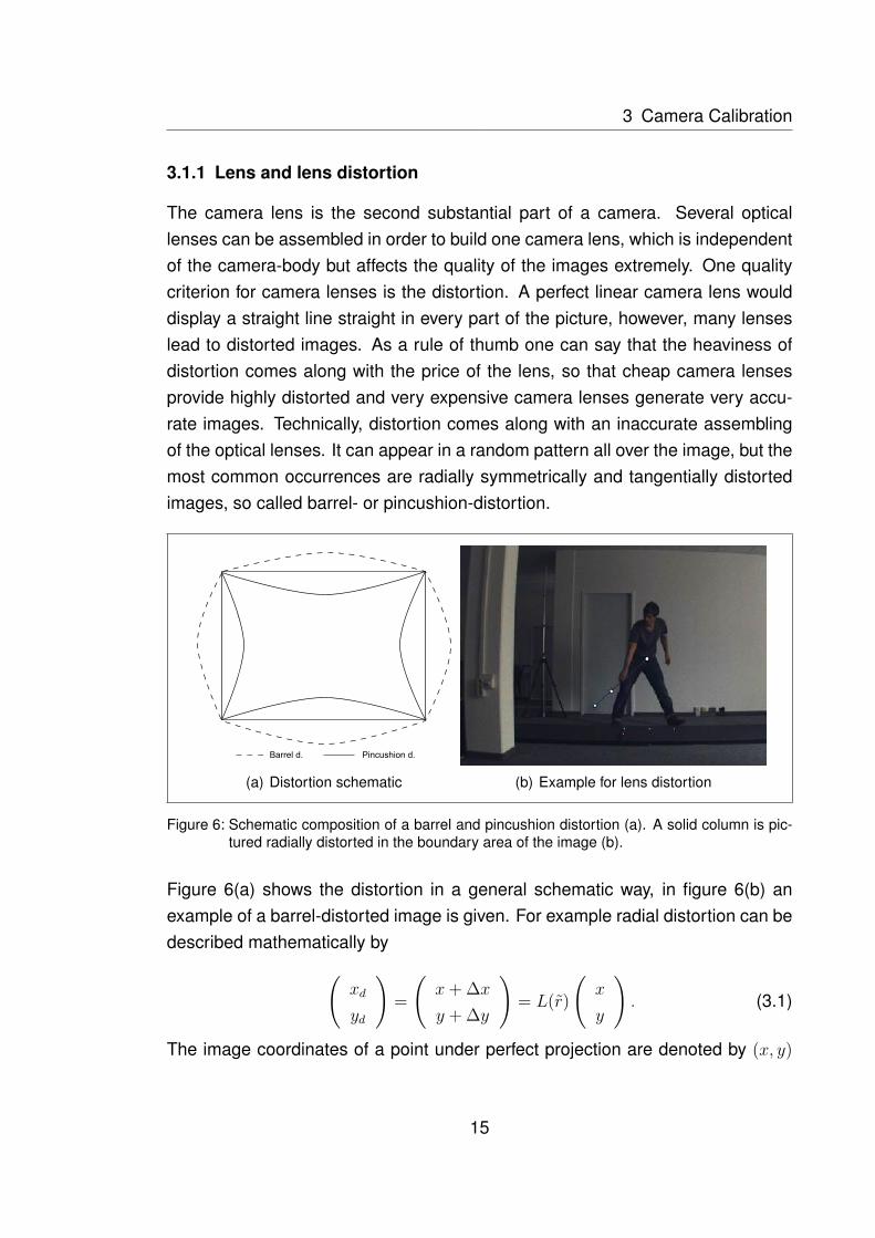
The camera lens is the second substantial part of a camera. Several opticallenses can be assembled in order to build one camera lens, which is independentof the camera-body but affects the quality of the images extremely. One qualitycriterion for camera lenses is the distortion. A perfect linear camera lens woulddisplay a straight line straight in every part of the picture, however, many lenseslead to distorted images. As a rule of thumb one can say that the heaviness ofdistortion comes along with the price of the lens, so that cheap camera lensesprovide highly distorted and very expensive camera lenses generate very accu-rate images. Technically, distortion comes along with an inaccurate assemblingof the optical lenses. It can appear in a random pattern all over the image, but themost common occurrences are radially symmetrically and tangentially distortedimages, so called barrel- or pincushion-distortion.

(a) Distortion schematic (b) Example for lens distortion

Figure 6: Schematic composition of a barrel and pincushion distortion (a). A solid column is pic-tured radially distorted in the boundary area of the image (b).

Figure 6(a) shows the distortion in a general schematic way, in figure 6(b) anexample of a barrel-distorted image is given. For example radial distortion can bedescribed mathematically by(

xd

yd

)=

(x+ ∆x

y + ∆y

)= L(r)

(x

y

). (3.1)

The image coordinates of a point under perfect projection are denoted by (x, y)

15


and (xd, yd) are the actually measured image coordinates containing radial distor-tion. The difference between the perfect and the projected point in x- respectivey-direction is (∆x,∆y) and r =

√x2 + y2 denotes the radial distance from the

center of radial distortion. L(r) is distortion factor as a function of the radius r.(cf. Hartley and Zisserman, 2003, ch. 7.4)Those kind of distortions can be corrected quite well during the calibration of thecamera. A possible way to correct the distortion is briefly presented in section3.3.

3.2 Camera Models

In terms of image processing and computer vision the technical composition ofa camera needs to be transferred to a mathematical model. Generally, everymodel of a camera is based upon the standard pinhole model, a principal of cen-tral projection like presented in figure 1. This model maps every X ∈ R3 to itscorresponding x ∈ R2 and can be described with

x = PX (3.2)

using the homogeneous representation x ∈ R3 and X ∈ R4 of 2D image pointand the corresponding 3D world point. P ∈ R3×4 is called the camera projectionmatrix, which describes the relation of a 3D point to its 2D representation on theimage plane.An idea of the geometrical interpretation of a pinhole camera is given by figure7 where the properties of the intercept theorem are used to compute a virtualimage plane in order to simplify the drawing in comparison to figure 1. A 3D pointis mapped to the image plan for a given focal length f via

(X, Y, Z)→ (fX/Z, fY/Z) (3.3)

which can be shown with basic geometric tools. To write down this basic mappingwith respect to equation (3.2), equation (3.3) can be transferred to a matrix-vectornotation with homogeneous coordinates.

16


(a) Projection 3D (b) Projection 2D

Figure 7: Geometry of a pinhole camera in a 3D (a) and in a 2D view (b). C denotes the cameracenter and P is the principal point. XW is the 3D world coordinate and XI its correspond-ing 2D image plane coordinate. (acc. Hartley and Zisserman, 2003, p. 154)

X

Y

Z

1

7→ fX

fY

Z

=

f 0f 0

1 0

︸︷︷︸

=P

X

Y

Z

1

. (3.4)

The matrix P can be expressed in a more simple way with

P = diag(f, f, 1)[I|0] (3.5)

where diag(f, f, 1) is a diagonal matrix and [I|0] a matrix split up into a 3 × 3

identity matrix plus an extra column vector containing only zeros. P is the cameraprojection matrix for the basic pinhole model. This model can now be expanded toattain the camera model used for the purpose of this thesis, a CCD like projectivecamera model.The pinhole model assumes that the origin of the image plane is the principalpoint, the center of the image. In practice one might find the origin at other loca-tions, and the used model is required to handle such drifts. With inhomogeneouscoordinates this problem would lead to

(X, Y, Z)→ (fX/Z + px, fY/Z + py) (3.6)

17


with (px, py) ∈ R2 being the coordinates of the principal point. In homogeneousrepresentation equation (3.6) is written as

X

Y

Z

1

→ fX + px

fY + py

Z

=

f px 0f py 0

1 0

︸︷︷︸

=K

X

Y

Z

1

. (3.7)

The matrix K is called the camera calibration matrix and f, px, py the intrinsic orinternal camera parameter.In practice the orientation of the camera coordinate system and the world coor-dinate systems differ and can be described via a rotation R and/or a translationt. Figure 8 gives an idea of this, where Xw = (Xw, Yw, Zw) expresses the coordi-nates of a point in the world coordinate system and Xcam = (Xcam, Ycam, Zcam) thecoordinates of a point in the camera coordinate system.

Figure 8: Euclidean transformation of world coordinates to camera coordinates, (acc. Hartley andZisserman, 2003, p. 156)

Such a transformation can be expressed in homogeneous representation as

18


Xcam =

Xcam

Ycam

Zcam

1

=

[R t

0 1

]Xw

Yw

Zw

1

=

[R t

0 1

]Xw. (3.8)

R ∈ R3×3 is a 3D rotation matrix with the property

R = Rx(θx)Ry(θy)Rz(θz). (3.9)

Rx, Ry, Rz ∈ R3×3 are the rotation matrices for the three axes with angle θ ∈[0◦, 360◦]. With t = −RC and C ∈ R3 being the coordinates of the camera centerregarding the world coordinate system, the orientation of a camera is completelydescribed. The parameters θx, θy, θz, t are called the external or extrinsic parame-ters. Combining equations (3.2), (3.7), and (3.8), a general mapping of a pinholecamera, placed arbitrary in the 3D world, is defined by

x = K[R | t]X. (3.10)

This camera model has nine degrees of freedom. Three internal (f, px, py), threeexternal for the rotation around the different axis (θx, θy, θz) and three external forthe translation of the origin (C).Given the transformation of the world coordinate system to the camera coordinatesystem, as illustrated in figure 8 a simple example for the orientation of a cameracan be presented.

19


Example: Assume a translation of −100 pixel in x-direction, 10 in y-directionand 0 in z-direction of the origin of the world system according tothe camera system. Thus t = (−100, 50, 10)t. The rotation of thecoordinate system is given with a counter clockwise rotation θx =

90◦ = π2

around the X-axis and a counter clockwise rotation θy =

180◦ = π around the rotated Y -axis.

Rx =

1 0 0

0 cos(θx) sin(θx)

0 − sin(θx) cos(θx)

, Ry =

cos(θy) 0 − sin(θy)

0 1 0

sin(θy) 0 cos(θy)

Rx and Ry are the corresponding rotation matrices in the 3D space.Since the rotation is multiplicative, the rotation matrix R and transla-tion t for this transformation in terms of equation 3.8 is

R = RxRy =

−1 0 0

0 0 −1

0 −1 0

and t = Rt =

100

−10

−50

.

Since CCD like cameras usual have non square pixels and thus different num-bers of pixels per unit distance according to the image coordinates, mx and my

are introduced as the number of pixel per length unit in x- respective y-axis direc-tion. The representation of the focal length with respect to the pixel dimension isthen given by αx = fmx and αy = fmy. Equivalently one can transfer the principalpoint (x0, y0) = (mxpx,mypy) to be the principal point in pixel dimensions.Thus, the calibration matrix of a finite projective camera, which equals a CCD-camera, is given by

K =

αx s x0

αy y0

1

. (3.11)

The parameter s is called a skew parameter and is equal to zero in most cases.There are two general options for this skew parameter to become non-zero. Thefirst, more unlikely option, is a skewing of the pixel elements in the CCD array.This means that the x- and y- axis are not perpendicular. The second, morecommon option can appear if taking a picture of a picture for example.

20


With a calibration matrix like in equation (3.11) the projection matrix P for a finiteprojective camera can be written as

P = K[R|t] =

p11 p12 p13 p14

p21 p22 p23 p24

p31 p32 p33 p34

. (3.12)

This projection matrix P has eleven degrees of freedom, like an arbitrary 3 × 4

matrix, it is defined up to scale, which comes along with the properties of homo-geneous coordinates. This means, the determination of eleven parameters of Pwill result the twelfth parameter automatically.The derivation of the camera models is a necessary step in order to extract datafrom existing images. Every basic book concerning computer vision respectivephotogrammetry has a good approach of those models. As an example the refer-ences of this section are mentioned. Hartley and Zisserman (2003, ch. 6), Klette,Schlüns, and Koschan (2001, ch. 2), and Faugeras (2001, ch. 3) provide all a verygood overview of the mathematical models of a camera.

3.3 Calibration

"Camera Calibration in the context of three-dimensional (3D) machine vision is theprocess of determining the internal camera geometric and optical characteristics(intrinsic parameters) and/or the 3D position and orientation of the camera framerelative to a certain world coordinate system (extrinsic parameters)". (Tsai, 1987, p.323)

In general calibration is the process of determining the parameters for the pro-jection matrix P from equation (3.2). For a multi camera system this has to bedone for every camera, but with respect to the whole system. The internal andexternal parameters are derived from the information provided by the mappingsof image points and control points. There are several approaches for the calibra-tion of a camera. This section provides an overview of two common methods forcalibration of a multi camera system, a static and a dynamic one.For every method the standard approach and its practical application, the tech-nical aspects are described, followed by the theoretical aspects of the calibration

21


technique. As far as further information are not needed for a better understand-ing in this section, informations about specifications of certain tools, like distancesare not given. Later on, in section 5.1, when the tests and used methods for theverification are presented, the specifications and dimensions of the used objectsare specified.

3.3.1 Static calibration

The static calibration is a well known calibration method for camera systems.Following, the technical and theoretical aspects for this method are presented.The software used for this description is SIMI Motion v. 8.0.317 (Motion).

3.3.1.1 Technical aspects

The method used for the calibration with the SIMI software at present is a staticcalibration based on a direct linear transformation (DLT, compare section 3.3.1.2).Tests were conducted following the manual "Working with 3D Data" (SIMI, 2005)and from experiences gained during the work for this thesis. A rigid calibrationdevice with at least eight known metric information, control points, is used for thiscalibration. Most times a cuboid like construction is used. Figure 11 shows sucha device, which is the calibration device used for testing at the SIMI laboratory.The motion analysis software SIMI Motion provides the possibility of static calibra-tion. Important notes for the calibration are that every camera of a multi camerasystem is calibrated independent of the other cameras. Further, the calibrationobject should fill the whole picture, or at least the area of interest which is neededfor the analysis.The step by step approach in SIMI Motion to calibrate a system using the staticcalibration is:

1. specify calibration object in Motion by creating virtual 3D control points2. record calibration video of the calibration object3. match control points with related 2D image points4. select calibration method (cf. table 1)5. check whether calibration was successful or not6. end calibration or return to step 2

22


Specifying the control points can be thought of telling the software the dimensionsof the calibration device. A 1m × 1.5m × 2m calibration cube could define eightcontrol points which can be denoted for example by

X1 = (0, 0, 0), X2 = (1, 0, 0), X3 = (0, 1.5, 0), X4 = (1, 1.5, 0),

X5 = (0, 0, 2), X6 = (1, 0, 2), X3 = (0, 1.5, 2), X8 = (1, 1.5, 2).

A video of the calibration object is needed to match the control points to the cor-responding 2D image points. All cameras should picture the whole calibrationdevice and the matching of the control points needs to be as accurate as possibleto avoid an invalid calibration. Already small errors in the coordinates of the con-trol points can lead to useless calibration results (cf. Lavest, Viala, and Dhome,1998).Selecting a calibration method sets the accuracy of the calibration. Different DLTmethods will yield different numbers of calibration parameters. The eleven pa-rameters for extrinsic and intrinsic are provided with every method. Additionalparameters for correction of distortion are possible, but also need a various num-ber of control points (cf. table 1).

Table 1: Different calibration methods used in SIMI Motion

Calibration method Min. number of control points neededDLT 11 8DLT 12 10DLT 14 12DLT 16 14

When the matching is finished, there are some optional settings, like the cam-era positions (extrinsic parameters), which can be set if they are known exactly,but will also be determined within the calculation of the calibration. When thematching of the image points and the control points and settings are done, theparameters of the DLT are computed automatically and the calibration process isfinished. SIMI Motion provides a calibration check where the relations betweenthe 2D coordinates of the control points and the reprojected 3D coordinates ac-cording to the resulting calibration is computed. If the calibration was not accurateenough the user gets a notification and the calibration should be repeated. One

23


of the most common errors for a failed calibration is switching two or more controlpoints.

3.3.1.2 Theoretical aspects

In this theoretical part the mathematical aspects regarding the static camera cal-ibration are presented. In 1971 Abdel-Aziz and Karara introduced a "method forphotogrammetric data reduction without the necessity for neither fiducial marksnor initial approximations for inner and outer orientation parameters of the cam-era" (Abdel-Aziz and Karara, 1971, p. 1). The concept presented in their work iscalled the Direct Linear Transformation (DLT) and has become a standard methodfor the calibration of cameras. A basic idea of what the DLT is about is given nowaccording to Abdel-Aziz and Karara (1971), the illustration of Kwon (1998) andthe book of Wöhler (2009).

In order to obtain the parameters for the orientation, the DLT uses informationgained from the correspondences of the control and image points. This methodis based upon the collinearity condition. To derive this condition, one might re-call figure 1 and assume the projection center C = (x0, y0, z0) and an arbitrary3D world point Xw = (x, y, z) with respect to the world coordinate system (XY Z).The corresponding image point XI = (u, v) is given with respect to the imagecoordinate system (UV ).A third, virtual axis W can be added to the UV -system, pointing in the directionof the projection center C. For points in the image plane one might set w = 0 andreceive XI = (u, v, 0). Further the principal point P = (u0, v0, 0) and the projectioncenter C = (u0, v0, f) might be set with respect to the new UVW -system, and f

denotes the focal length of the camera.

Two vectors ~A = Xw − C and ~B = XI − C can be defined.

~A = Xw − C =

x− x0y − y0z − z0

, ~B = XI − C =

u− u0v − v0−f

(3.13)

The collinearity of C (which is equal to C), Xw and XI can be seen in figure 1. Thus

24


~A and ~B form a straight line which can be expressed by

~B = c ~A (3.14)

with c ∈ R being a scalar scaling factor. Since ~A and ~B are described both indifferent coordinate systems, a transformation is needed to express both of themin relation to the same coordinate system (cf. figure 8).

ITw = Rx Ry Rz =

r11 r12 r13

r21 r22 r23

r31 r32 r33

(3.15)

describes a general transformation matrix (rotation) for a vector from the worldcoordinate system to the image coordinate system. Rx, Ry and Rz are the 3Drotation matrices for the x-, y- and z-axis respectively. ~AI and ~Aw denote therepresentation of ~A in the image coordinate system and the world coordinatesystem, respectively. The coordinate transformation can be executed by

~AI = ITw ~Aw. (3.16)

Combining equation (3.14) and (3.16) yields u− u0v − v0−f

= c

r11 r12 r13

r21 r22 r23

r31 r32 r33

x− x0

y − y0z − z0

(3.17)

or, resolving the matrix vector multiplication,

u− u0 = c(r11(x− x0) + r12(y − y0) + r13(z − z0))v − v0 = c(r21(x− x0) + r22(y − y0) + r23(z − z0))−f = c(r31(x− x0) + r32(y − y0) + r33(z − z0)).

(3.18)

Equation (3.18) can be resolved and substituted for c to obtain

u− u0 = −f r11(x−x0)+r12(y−y0)+r13(z−z0)r31(x−x0)+r32(y−y0)+r33(z−z0)

v − v0 = −f r21(x−x0)+r22(y−y0)+r23(z−z0)r31(x−x0)+r32(y−y0)+r33(z−z0)

. (3.19)

Equation (3.19) can be rearranged to obtain expressions for u and v dependingon x, y and z with eleven constant parameters:

25


u = L1x+L2y+L3z+L4

L9x+L10y+L11z+1

v = L5x+L6y+L7z+L8

L9x+L10y+L11z+1

(3.20)

D = −(x0r31 + y0r32 + z0r33), (du, dv) = ( fλu, fλv

),

L1 = u0r31−dur11D

, L2 = u0r32−dur12D

, L3 = u0r33−dur13D

,

L4 = (fur11−u0r31)x0+(dur12−u0r32)y0+(dur13−u0r33)z0D

,

L5 = v0r31−dvr21D

, L6 = v0r32−dvr22D

, L7 = v0r33−dvr23D

,

L8 = (dvr21−v0r31)x0+(dvr22−v0r32)y0+(dvr23−v0r33)z0D

,

L9 = r31D, L10 = r32

D, L11 = r33

D.

L1 − L11 are called the DLT parameters and express the relation between theworld coordinate system and the image plane according to the intrinsic and ex-trinsic camera parameters. λu and λv are conversion factors needed to transfermetric real world data into image data in pixel length unit.

In section 3.1.1 disturbed images due to radial or tangential lens distortion werementioned as a problem for photogrammetric applications. The DLT method canbe expanded and results in five more parameters L12 − L16, which describe re-spective correct the lens distortion. However, this expansion is no longer a lineartransformation but a non-linear iterative optimization step. According to Wood andMarshall (1986) this approach was first proposed in 1975 by Marzan and Karara.The equations for the 16 DLT parameters can be applied to an arbitrary numbern ∈ N of control points and will result in a system of linear equations (SLE) in thegeneral form of:

CL = I

C ∈ R2n×16, I ∈ R2n×1, L = (L1, . . . , L16)t.

(3.21)

C contains informations about resolved parameters from equation (3.20) joinedwith the 3D coordinates of the calibration device, and I similar provides informa-tion about the corresponding 2D image coordinates.To solve a SLE like (3.21) with 16 unknown, at least 16 linearly independent equa-tions are needed. Since every point correspondence results in two equations,one for the x- and one for the y-coordinate, at least eight non co-planar pointcorrespondences are needed to resolve the 16 DLT parameters. More points are

26


desirable since those points are not free of errors. To solve equation (3.21) inorder to obtain the DLT parameters a least squares method can be used.It is common not to compute all 16 DLT parameters for calibration due to thelack of a sufficient calibration device for example. Frequently used and feasiblesubsets of the 16 DLT parameters are summarized in table 2, combined with theminimal number of required points and some remarks on the additional parame-ters.

Table 2: Different DLT subsets

Subset DLT Parameters Min. pts req. RemarksDLT 11 L1 − L11 6 Standard DLT parametersDLT 12 L1 − L12 6 DLT 11 + 3rd order optical distortion termDLT 14 L1 − L14 7 DLT 12 + 5th-, 7th- order optical distortion termsDLT 16 L1 − L16 8 DLT 14 + tangential distortion terms

Kwon (1998, 3-D DLT Method)

The difference between the needed points in the SIMI software (cf. table 1) andthe minimal number of needed points can be explained by the accuracy of thecalibration in order to reduce influence of errors for the computations.For a more detailed look at the modeling of the optical error and solving of theDLT one might consider to check the related literature mentioned in the beginningof this section.

3.3.2 Dynamic calibration

As described in section 3.3.1.1 the manageability and inflexibility of the calibra-tion device can be a problem of the static calibration. In order to avoid using suchrigid objects, new more user-friendly calibration methods are needed. In 1992Faugeras, Luong, and Maxbank provided an approach to calibrate a camera’sintrinsic parameters by just using point correspondences. In this method, calledself-calibration, the 3D geometry is recovered using the 2D images of a singlemoving camera. Since picturing a static object with a moving camera is equiv-alent to recording a moving object with a static camera, the idea of a dynamiccalibration is given.

27


Dynamic calibration is generally performed by waving a wand of known size inthe area of interest. This easy to use calibration technique is already a commonlyused method and is available for different systems like for example ART (2011),OptiTrack (2011) or Vicon (2011). The general approach of this calibration methodand the basic mathematical background of it is provided now.

3.3.2.1 Technical aspects

For the algorithm used for this work, a wand of known size, with three markersattached, and a L-frame with four markers are needed (cf. section 5.1.2). Thewand, also called T-frame, is needed for calibration of the area of interest and ismoved around this area during the calibration process. The L-frame is used toset the origin and coordinate axes of the reference system and is placed at thedesired place.Important aspects for the dynamic calibration are that the whole T- and the L-frame must be recorded by at least two cameras at each time in order to create avalid picture for the calibration (cf. epipolar geometry, section 2.5). The practicalusage of the wand calibration as a step-by-step approach used in this work is:

1. set global coordinate system by placing the L-frame at the desired place ofthe pictured area and start recording the calibration video for every camerasimultaneously

2. cover the L-frame3. wand the area of interest with the T-frame and stop recording4. track data and export 2D coordinates of T- and L-frame5. initialize and run wand calibration algorithm6. check calibration and import to Motion

Since the wand calibration is still being tested and is not included to the SIMIMotion yet, this approach was used as a workaround for this thesis. The workof an end user should end at step 3 in the final implementation and steps 4 - 6should be executed automatically. Nevertheless, the tracking will be the same asit will be done in the end version and the other aspects have no affects on theresults and calibrations at all.A global reference coordinate system is need to be able to reconstruct data fromthe obtained data. For the static calibration one can define those orientations by

28


the rigid body used for the calibration. Since there is only a waving wand, thedynamic calibration uses a L-shaped device placed at the desirable origin to setthe reference system. The two arms of the L-frame indicate the X- and Y -axisof the reference coordinate system and the Z-axis is computed automatically.Section 3.3.2.3 provides a more detailed look on this topic.Instead of moving the L-frame out of the area of interest, the frame is just coveredwith a sheet to avoid the possibility of jumping markers during the further calibra-tion process when moving the T-frame close to the L-frame. Moving the T-framearound the pictured space is called wanding or performing a wand dance. To findthe best way of wanding in order to get a good calibration is part of this work andis reviewed when the results of the test are discussed in chapter 7.Tracking the wand is the most important step on the way to a good calibration. Itcan be done either manually or automatically, though practical experience showedthat the automatic tracker is more accurate than the manual tracking process andis thus chosen as the tracking option for this thesis.For practical use nothing more than initializing the algorithm with the length of thewand, the ratio of accuracy and the number of cameras as well as their aspectratio is needed. Hereby, the ratio of accuracy describes the number of camerasthe wand has to be seen in at the same time to be accounted for calibration, thenumbers of frames used (from all the valid frames) and the number of optimizationsteps.

3.3.2.2 Theoretical aspects

The theoretical background of the tested wand calibration is based upon the workof Mitchelson (2003). Remembering the fact that calibration is the determinationof the projection matrices Pi for each camera if correction of distortion is notincluded, it is obvious that calibration of a multi camera system with M camerasequals finding the projection matrices P1 . . . PM for the different cameras. Withknowledge about epipolar geometry (section 2.5) a 3D point can be reconstructedif the position of a point is found in a sufficient amount of views, which is two viewsor more if the principal rays are not collinear. Being able to find a given distance,this means having the position data of two points per camera, and knowing thelength of this distance in the real world an optimization process using the given

29


length as a constraint can yield a valid calibration for the multi camera system.Besides the capturing of data there are three main technical steps in order to do adynamic calibration, extraction of the features, initialization of the calibration, andoptimization.The extraction of the features of the recorded videos is the determination of theposition of a marker. Since a marker is not defined by a single pixel in general,the center of a marker is used as its position (compare step 4 for the dynamiccalibration). For the purpose of this thesis the existing automatic tracking featureof SIMI Motion was used. Compared to the work of Mitchelson, where a wandwith two colored markers is used to uniquely identify each marker, a bar with threereflective markers is used. The two outside markers determine the length of thewand and the third, the middle marker, is used for the identification process. Themiddle marker sections the wand in a given ratio, for example 1 : 2 or 1 : 3 to allowa unique identification. With respect to the properties of projective geometry,calculations proofed a segmentation of 1 : 2 as a sufficient segmentation whichleads always to a unique identification of the markers (Henrici, 2011). During thework of this thesis this ratio also turned out to be the optimal setting for calibration.Since the wand calibration algorithm only worked with presorted points in thebeginning, an existing point sorting and validation algorithm was added to thewand calibration during this thesis. The algorithm processes a set of input data,image coordinates for the wand and L-frame in a random order, and results asorted valid data set, split up into wand and static points.The second main function of the algorithm is the validation of the input data. Es-pecially for the wand data a lot of invalid data can occur. Distortion and inaccuratetracking could lead to problems for the computation of a valid calibration. Thusthe input data are checked whether they fulfill some criteria with respect to a giventolerance for each value. The input data for the wand are checked mainly for theircollinearity and if the sum of the two segments of the wand equals the total lengthof the wand.The initialization of the calibration is done with the information gained from thefundamental matrices Fi (cf. section 2.5). Hartley (1992) presented a linear al-gorithm to compute the fundamental matrix from point correspondences of twoviews from uncalibrated cameras, based on the work of Longuet-Higgins. Forthis algorithm only eight point correspondences are needed in order to compute

30


a valid result, thus it is called the 8-point algorithm (Hartley, 1992, p. 1). Morepoints would add no further information but will lead to more numerical stability ofthe computation.The 8-point algorithm is said to be very sensitive to noise, so Hartley (1995)provided a more numerical stable update of this algorithm for the computation ofthe fundamental matrices.One camera is supposed to be at the world origin and the second one is placedarbitrarily in the 3D space. The corresponding fundamental matrix is then com-puted for every camera pair of the multi-camera system which has to be cali-brated. For a system with N cameras this will result in N(N − 1) fundamentalmatrices, but due to the relation xtFx′ = 0⇒ x′tF tx = 0 the computational affordcan be reduced to the computation of N(N − 1)/2 fundamental matrices.The next step towards the estimation of a calibration is a first guess of the focallength of each camera. Again Hartley (1993) provided an approach to extractthe approximate focal length from the fundamental matrix F from the aspect ra-tio and the principal points of each camera. The fundamental matrix F can bedecomposed into

F = Kt1R[µt]×K2. (3.22)

Hereby, K1, K2 denote the internal parameters of the two cameras under consid-eration (cf. equation 3.11), R, t is a translation and rotation from one camera tothe other (cf. 3.8) and µ ∈ R+\{0} is a scaling factor. Knowing K1 and K2 theextraction of R and µt is possible for a given F and the focal lengths of the twocameras can be estimated if the the principal point and aspect ratio are given(Mitchelson, 2003, sec. 3.4.3). The aspect ratio is given as a needed input for thealgorithm and the principal point is set to the center of an image as a first guessif not known exactly and will be optimized during the further computations.Assuming now an estimate guess of the camera parameters to be given, an opti-mization process yields the final calibration. The optimization is needed since themeasured image points are afflicted with some noise in general. A possible func-tion to be minimized is a geometric error which expresses the sum of squarederrors between a reconstructed and an actual measured point. This error indi-cates the euclidean distance between two points in a 2D image space. The ith

31


measured point is denoted by xi = (ui, vi)t and the ith reconstructed point by

xi = (ui, vi)t. The geometric error is then given by

errgeo =

√√√√ N∑i=1

|xi − xi|2 (3.23)

with N being the total amount of observations. With respect to the numericaleffort and the property that

min√x⇔ minx, x ∈ R+ (3.24)

holds true, it is sufficient to use only

errgeo =N∑i=1

|xi − xi|2 =N∑i=1

|ui − ui|2 + |vi − vi|2 (3.25)

for the optimization process. The geometric error shall be minimized with respectto all M views and thus it is extended for the wand calibration to

errgeo =N∑i=1

M∑j=1

|xij − xij|2. (3.26)

for the optimization process. Minimizing this non linear optimization problem canbe done iteratively using descent methods. A commonly used method for solv-ing such problems is the Levenberg-Marquardt algorithm, a modification of theGauss-Newton method.Such a problem which estimates the calibration and reconstruction parameters asa result of minimizing some cost functions for several views is also called bundleadjustment (Triggs, McLauchlan, Hartley, and Fitzgibbon, 2000, pp. 1-2). For amore detailed look at the mathematical derivation and proofs for the presentedconcepts the underlying literature for this section is recommended like Hartleyand Zisserman (2003, ch. 18 and appendix 5) or Mitchelson (2003, ch. 3). Amore more application-oriented view is given in Luhmann (2010, sec. 4.) for thistopic.

32


3.3.2.3 Computation of the World Coordinate System

For most applications it is desired to have the world origin at a given place. Thewand calibration with the T-frame only would set the origin to the center of oneof the cameras. As described in the previous section the setting of the world co-ordinate system is technically done by a rectangular L-frame, which is placed atthe chosen origin of the coordinate system. Since the first version of the wandcalibration algorithm only handled presorted image points for the wand and theL-frame an automation for the computation of the coordinate axes and the sort-ing of the static points for all cameras was implemented during this work and isdescribed now.Given the eight 2D coordinates of four static points for each camera, one couldplot a picture like figure 9. As it can be seen every camera provides a projectionof the L-frame, where the dots represent the position of a marker and dots of thesame color are pictured by the same camera. For this work the X-axis is set tobe the direction of the three collinear points and the Y -axis to be the short arm ofthe L-frame.

0.25 0.3 0.35 0.4 0.45 0.5 0.55 0.6 0.65 0.70.35

0.4

0.45

0.5

0.55

0.6

0.65

0.7

in %

in %

Figure 9: Coordinate system reference tool pictured from four different views. Each group of col-ored dots represents the L-frame from one view. The datas are normalized to the widthrespective the height of the picture

The properties of the projective geometry yield that collinear points stay collinear(Hartley and Zisserman, 2003, p. 44). Nevertheless collinearity could be de-stroyed by lens distortion, and thus the identification could yield some problems.One option to solve this problem, as practiced in this work but not always possi-

33


ble, is the correction of the distortion of the videos before further computationsare made. If no distortion correction is possible, some tolerances for the com-putations shall be allowed in order to achieve a valid sorting of the static points.However, even for corrected images those tolerances shall be allowed too, in caseof slight tracking errors due to noise for example.Another problem could be that all four static points become collinear. But this willonly happen if the center of projection lies on the plane defined by the two axis ofthe L-frame for each camera. This would be equivalent with a camera mountedon the floor at the same height as the L-frame, an uncommon setting for thosekind of systems and thus can be neglected.For the rest of this section the homogeneous points of the L-frame are given byx1,x2,x3,x4 ∈ R3 in an arbitrary order.Without any knowledge of distances and angles there are always two points thatare clearly identifiable for each camera. This is the stand alone point and themiddle point, as it can be seen in figure 9.A line l ∈ R3, containing two arbitrary points xi,xj, i 6= j, can be computed usingthe cross product: l = xi× xj. If a point xk lies on this line, xtkl = 0 holds true. Forthe purpose of this work a tolerance, TOLd ∈ R+\{0} for this equation is neededsince noise and tracking can result in small errors for the static point coordinates.Hence three collinear points can be found iterative with

xtkl = xtk(xi × xj) ≤ TOLd, i, j, k ∈ {1, 2, 3, 4} (3.27)

and an appropriate tolerance. Let the points found this way be x2,x3,x4 and setx1 to be the stand alone point. The middle point of this set of three points can nowbe found easily by comparing the length of the vectors between each two-pointpair xi,xj, i 6= j, i, j ∈ {2, 3, 4}. A vector ~vxy ∈ Rn between two points x, y ∈ Rn iscomputed with ~vxy = xt − yt and for three points x, y, z ∈ Rn, with middle point z,equation (3.28) has to be true.

‖ ~vxz + ~vzy ‖2 = ‖ ~vxz ‖2 + ‖ ~vzy ‖2 (3.28)

Hereby is

34


‖ ~x ‖2 =

√√√√ n∑k=1

|xi |2, ~x ∈ Rn (3.29)

the euclidean norm of a vector, which can be interpreted as the length of the vec-tor. Thus, the middle point can be found iteratively and is set to be x4.

The identification of x2 and x3, the origin and the point at the very end of the X-axis direction, is missing. Because of projective images, no more information canbe gained from a 2D picture of a single view. To finish the identification of thosepoints, 3D data from the static points need to be reconstructed. The 3D data canalready be computed with the projection matrices Pi ∈ R3×4 (cf. 3.2) computed bythe wand calibration since they already yield a valid calibration. Only the correctorientation of the world coordinate system is missing but lengths and angles arecomputed in the correct dimensions. With those reconstructed coordinates, Xi

is the 3D representation of xi, it is possible to compute a three point angle andthe 3D world lengths of the L-frame to find the missing information for the set ofstatic points. Since cameras could be arranged in a way making it impossible toreconstruct 3D data, for example collinear principal rays, an iterative approach isneeded for a valid reconstruction.

(a) (b)

Figure 10: The two possibilities for angles with the unknown points from a top view.

With the setting of the calibration object one can derive α = 90◦ and β � 90◦

for the angles visualized in figure 10 to finish the identification. With the dotproduct (3.30) the 3-point angle can easily be computed to recieve the missinginformation.

~v1 · ~v2 = ‖ ~v1 ‖2 ‖ ~v2 ‖2 cos(~v1, ~v2) (3.30)

35


Again a tolerance TOLa ∈ R+\{0} is needed with respect to the noise and track-ing errors to fulfill this condition. Since cos(90◦) = 0, the rectangular angle can befound with

cos(~vx1xi , ~vx4xi) =‖ ~vx1xi ‖2‖ ~vx4xi ‖2

~vx1xi~vxix4≤ TOLa, i = 2, 3 (3.31)

and the identification of the last two points is finished. With a careful choice ofTOLa and a verification of the known lengths of the arms of the reconstructedL-frame exactly one solution exists. Let this solution be x2 and denote it as theorigin of the reference system. The last point is x3, which is the outside point ofthe X-axis direction. Thus ~vx = ~vx3x2 can be defined as the X-axis direction and~vy = ~vx1x2 as the Y -axis direction.The last step in order to compute the world coordinate system is to find the Z-axis.By definition of a Cartesian coordinate system the axis are perpendicular to eachother. Since the cross product (cf. equation (2.3)) yields a vector perpendicularto the two input vectors, the direction of the Z-axis can be computed. This can bedone, again with the help of the cross product

~vz = ~vx × ~vy. (3.32)

To assure orthogonality the direction of the Y -axis can be recomputed with

~vy = ~vz × ~vx (3.33)

and the old value is updated with ~vy to get a coordinate system with accuraterectangular angles.Equations (3.32) and (3.33) are defined with regards to a left handed coordinatesystem like it is commonly used in motion analysis. To transfer those equations toa right handed coordinate system one needs to adjust the calculations accordingthe property of the cross product provided in equation (2.6).

36

4 Related work and theory construction

As seen in the introductory part of this thesis, section 1.2, the validation of acalibration equals the analysis of accuracy of the given calibration. In this chapteran overview of some existing studies of this topic is given in section 4.1 to allowfurther a purposive design of experiments for the validation, which is given insection 4.2.

4.1 Related work

The validation and analysis of accuracy for 3D motion analysis systems is a welldiscussed topic. Searching for evaluating and comparative studies on this topicresults in several papers, studies and proceedings of conferences. The vast ma-jority of these papers is dated to the ’90s. Due to an increasing hard- and soft-ware performance for such systems every year, results especially regarding theaccuracy should be considered critically and may be outdated, and are thus notpresented here. However, some of these investigations will be considered now,since the general methodology of these studies motivated the approach for thisthesis.Luhmann and Wendt stated in the context of optical 3D measuring systems that"In conformity to existing guidelines the error of length measurement is proposedas quality parameter to assess the geometric performance" (Luhmann and Wendt,2000, p. 500). Taking a fixed length as a reference for the accuracy of such anoptical system is a well known method. In 1994 Ehara, Fujimoto, Miyazaki, andYamamoto (1995) conducted a first test by comparing eight commercial available3D camera systems for clinical gait analysis. Among other things, like the pro-cessing time, they evaluated a calculated distance for three tracked markers fixedto a rigid bar as an indicator for accuracy.Already three years later Ehara, Fujimoto, Miyazaki, Mochimaru, Tanaka, andYamamoto (1997) repeated this study and tested eleven 3D systems for theiraccuracy. The used methods were similar to the ones used in the first tests butthe results differed already a lot due to the improvements of the systems.During the Comparison Meeting of Motion Analysis Systems (2002), held in Japanand organized by Ehara, several systems were tested again. Tests included the

37


methods realized by Ehara et al. (1997) in the recent studies, but for examplealso an angle was added as a measure, which was realized by attaching threemarkers to an L-shaped scale.The studies conducted by Ehara et al. provided a possibility to compare differentmovement analysis systems. However, these experiments should be reviewedcritically. For example, during the Comparison Meeting markers were attachedto the test device newly for every tested system and each system could be posi-tioned in a certain space arbitrary. Thus the comparability of different values fromdifferent systems lacks due to possible inaccuracies of attachment. Further noinformation is given about the spatial distribution of the measurements.A different approach to measure the accuracy of motion analyzing system is pro-vided by Richards (1999). A motorized device is placed in the center of the cali-brated volume to allow, amongst others, the measurement of a distance betweentwo markers fixed to rotating bar. Still, a fixed distance is taken as a reference,but a great advantage of the system used by Richards exists. This is the ability tomove markers on identical paths for each system if the location of the test deviceis equal for each system. Since the movement of the test device was limited rel-ative to the center of the motorized device, only a spatially restricted inspectionsof measures was possible.A more recent study, comparing the accuracy of two different calibrations, can befound for example from Pribanic, Peharec, and Medved (2009). A wand calibrationand a 2D plate calibration were compared by computing for example a distanceand an angle from one reference video with respect to each of the calibrations.Mitchelson and Hilton (2003) evaluated the performance of the wand calibrationdeveloped by Mitchelson (2003) in a similar manner. Considering the 2D repro-jection error and a reconstructed distance the wand calibration was compared tothe results gained by a checkerboard calibration.Further studies, like Vander Linden, Carlson, and Hubbard (1992), Wilson, Smith,and Gibson (1997), and Hatze (1988) refer to similar methods and results. How-ever, all of the presented studies in this section do have one thing in common,determining a single mean value for a distance or angle. No spatial inspectionof the distribution of the computed values can be found. Frantz et al. (2004) crit-ically reviewed this topic of a single value describing the accuracy of a whole 3Dtracking systems, which is done by most of the manufacturers of such systems.

38


A spatial examination of errors is proposed, as well as the consideration of otherstatistical values than the mean or root mean square only, for example the medianor 95% confidence intervals.A different design of experiments, which was more or less dynamic so far, is astatic tests. Those tests use different rigid bodies which are placed in the picturedspace and allow the measurements of distances assembled to the device andthe position of 3D coordinates. For example Arlt (1998) had a short look at theaccuracy of the SIMI Motion system with such a test setup during his work. Adrawback of this method is the reference object itself. The allocation of differentsized objects is not possible in any case and large testing volumes can hardly becovered by such an reference object. (Luhmann, 2010, sec. 7.2.3.3)

4.2 Theory construction

The conceptual idea for the formulated problem of the validation of the dynamiccalibration is to compare the accuracy of computed values in respect to theirground true values as this is a sufficient measure of the performance of 3D mea-suring system (Luhmann and Wendt, 2000). According to the methods used byEhara et al. (1997) for example, a special designed tool is used to measure sev-eral distances and angles for the different calibrations by moving this test devicethrough the entire pictured space. For a more detailed error evaluation a seg-mentation of the pictured space is used to provide a spatial error distribution withrespect to the work of Frantz et al. (2004).In order to check whether the dynamic calibration is an improvement to the exist-ing static calibration, results between the different calibration methods are com-pared as well.The different calibration methods can be considered the independent variablesof the tests. The dependent variables, the measures of the different values, arebased on the quality of the calibration. Thus, the results of the different measure-ments can be observed and used for a qualitative statement for the calibration.To collect those measures, the test tool is moved around the pictured space in away to cover the whole volume as good as possible.To allow fair testing and to eliminate the effect of different digitalization steps, onlyone reference video is chosen and the different calibrations are applied to it. This

39


allows a comparison between the different calibrations, which equals repeatedmeasurements respective comparing dependent samples. To minimize furtherthe effect of disturbing variables, the test are conducted in a special preparedlaboratory.

40

5 Methods and Materials

Subject of this thesis is to evaluate whether a new dynamic calibration methodmeets the expectations concerning accuracy or not. An adequate design of ex-periments was provided in section 4.2. This chapter concretizes this design andprovide all information about the materials and methods used for the validation.The first part, section 5.1, describes the tools used for calibration and for thetests. In section 5.2 and 5.3 the realization of the different test scenarios is de-scribed. The last part of this chapter, section 5.4, offers the needed informationabout computed error models.

5.1 Material

This section provides an overview of the specifications of the devices used for thecalibration and the testing.

5.1.1 Static calibration device

For the static calibration the QF-26 lightweight radiation calibration frame fromBeijing HuiAnMing Sciences Development Co. Ltd. was used. The calibrationframe, which can be seen in figure 11, is made of round aluminium tubes andneeds to be placed on a tripod. 16 rods can be assembled to span a maximumvolume of 1.69m× 1.69m× 1.31m. In total 26 plastic non reflective markers whichare used as control points for the calibration are attached to the rods.A smaller calibration frame can be created by using only eight rods spanning avolume of 0.87m× 0.86m× 0.66m, providing 17 control points for calibration.A specification file provides the metric distances of the different markers up to1mm accuracy. The origin of the world coordinate system is defined by one of theattached markers, according to the specification file.

5.1.2 Wand calibration and testing devices

For the wand calibration two calibration tools, the T-frame and a L-frame, wereconstructed for this work. Figure 12(a) and 13(a) show the calibration devices.

41


(a) Static calibration device (b) Static calibration device schematic

Figure 11: Picture (a) and schematic demonstration (b) of the static calibration device used for thetests.

The dimensions of the tools are shown in figure 12(b) and 13(b). The setup waschosen this way to allow different dimensioned tools for calibration and testingwith only one device.Some specifications of the different tools are listed below in a summarized form:

• T-frame (also called wand, fig. 12)

– Aluminium square tube: 15mm× 15mm× 1.5mm wall– Black painted surface– Attached markers: retroreflective spherical markers 15.9− 25.4mm, di-

ameter mounted with a M4 threaded bar

• L-frame (fig. 13)

– Aluminium square profile: 20mm× 20mm

– Black painted surface– Attached markers: retroreflective spherical markers 15.9 − 25.4mm di-

ameter, mounted with a M4 threaded bar

• Distance piece (fig. 12)

– Aluminium round tube: 8mm diameter, 1mm wall– Black painted surface

42


The construction of the tools was done as a part of this thesis. They were plannedin a way to allow a maximum variability for different test scenarios as well asproviding very accurate dimensions. Thus a specialized company produced thecalibration and test devices, according to the provided drawings, using a highaccurate computerized numerical control machine (CNC machine).

(a) T-frame/wand

100

Distancepiece

300

200

200

100 100100100100 50 100 [mm]50 505033.3

66.66 66.6633.3

1000

700

A

B

C D E

(b) T-frame schematic

Figure 12: Picture of the T-frame with a 1:2 segmentation used for the calibration (a) and aschematic sketching of its dimensions with the points A, B, C, D and E used for thetest setup (b).

(a) L-frame (b) L-frame schematic

Figure 13: Picture of the L-frame (a) and a schematic sketching of its dimensions (b).

43


The distance pieces are needed to mount the markers at a defined distance to theT-frame, otherwise the bar of the T-frame could occlude the markers frequently.Furthermore, the calibration tools were painted black to reduce reflections, whichcould wrongly indicate markers during the tracking process and to avoid extremelydisturbed datas.

5.1.2.1 Vicon T-frame

The calibration device used for the calibration of the Vicon system is shown in fig-ure 14. The used wand is the commonly used calibration wand for the laboratoryat the TU Munich, Institute of Ergonomics, where the tests with the Vicon systemwere conducted. The used T-frame contains five markers and is used for cali-brating as well as for setting the origin and orientation of the reference system.After wanding the area of interest the T-frame is placed at the desired place toset the world coordinate system. The wand, which has a length of ∼ 21cm, wassegmented with a 1 : 2 ratio by the attached retroreflective markers with 12.7mm

diameter.

Figure 14: Picture of the T-Frame used for calibrating the Vicon system.

5.2 Pretests

In order to get a good sense for the necessary test setup and the conditionsneeded for valid results some pretest were made. This testing and some of itsobservations which indicate to have effects on the tests are described now.First some existing videos, created for initial testing of the wand calibration, wereused to get a first idea of the algorithm. Those videos were shot by students at

44


the SIMI laboratory prior this work.As soon as the calibration devices, described in section 5.1.2, were available,new videos were recorded to find the best general conditions for the test setup.Most of the pretesting was done only with the wand calibration. One focus duringthese tests was to check whether some modifications of the calibration algorithmwere needed or not. Another important task was to find the specific disturbancevariables during the test and how to handle them the best for the main tests. Thecomponents used for the pretest setup are summarized in table 3.

Table 3: Materials used for the pretests

Quantity Material used4 AVT Pike F032c fiber camera with 640×480 pixels*4 Pentax H612A-KP 6mm lens*4 Tripod4 LED ring with 32 LEDs4 Optical fibre cable4 Trigger cable1 SIMI I/O Box 32 channel USB (Trigger Box)1 Computer system with SIMI Motion Version 8.0.3171 T-frame with 3 markers1 L-frame with 4 markers

*cf. appendix C

Figure 15 shows the arrangement of the cameras at the laboratory. All four cam-eras were placed on a tripod in ∼ 1.50m height, pointing slightly downwards to thecenter of the pictured space. Optical fibre cables were used to connect each cam-era to the computer system and a trigger cable was used to connect the camerasto the trigger box and energize the cameras and the LED rings, which were fixedto the cameras. The main task of the trigger box was to ensure synchrony record-ings, this includes starting the recordings at the same time, as well as assuringthat each single frames are synchrony.All windows of the laboratory were covered with curtains to avoid sunlight disturb-ing the measurement. The only active light sources were the LED rings attachedto the cameras. Other reflective objects like metallic surfaced objects were movedoutside of the area of interest.The setting of the wand was chosen with a distance of 1.00m and a ratio of 3 : 1.

45


Figure 15: Setup of the pretest. The grey area indicates the pictured area seen by at least twocameras.

A second setup was chosen with a wand length of 0.60m with a 2 : 1 ratio. TheL-frame was used with the settings shown in figure 13(b).After the preparations were finished the recording was started. The frequency ofthe recording was set to 100 frames per second (fps).

5.2.1 Observations of the pretests

After the recording of the videos and the evaluation of the obtained data someproblems for the usage of the wand calibration arose:

1. The whole wand is not pictured completely in a sufficient number of frames2. Bad calibration results in the upper part of the pictured space3. Most valid point triples are within the same area4. Difficulties during the tracking process:

a) Not enough contrast between markers and background in front of brightbackgrounds

b) Reflections/bright light sources indicate wrong markersc) Weak reflective markers in a too large distance to the camerad) Pictured markers appear too small when being too far away from the

camera

46


The first problem that the wand was not pictured completely in a sufficient numberof frames can be explained by the relation of the wand to the test setup. The twoouter points of the wand were 1.00m apart, which was good for pictures far awayfrom the camera or in the center of the pictured space. But invalid recordingsoccurred in an area very close to the camera, because the wand could not bepictured completely in a camera’s view. Thus the length of the wand needs to beadjusted to the size of the area of interest and to the arrangement of the cameras.The second problem can be explained by the distortion of the camera lenses. Ingeneral lens distortion is a problem in photogrammetry, compare section 3.1.1.Figure 16 shows the greatest errors, differences between the computed and theknown length, in the upper and boundary area of the pictured space. This canbe explained by lens distortion and could be corrected for example with higherquality lenses or a previous calibration of the distortion.

−2−1

01

23 −2

−1

0

1

2−0.5

0

0.5

1

1.5

Diff > 2.5cmDiff > 1.0cmDiff > 0.5cmDiff =< 0.5cm

(a) 3D space

−2 −1.5 −1 −0.5 0 0.5 1 1.5 2 2.5−0.2

0

0.2

0.4

0.6

0.8

1

1.2

1.4

1.6

(b) XZ-view

Figure 16: Difference of computed and real length in the 3D space (a) and in a 2D view of the X-and Z-axis (b) mapped to the middle point of the wand. The blue points indicate theglobal coordinate system. The errors are based upon distorted recordings.

The third problem, most valid point triples occur within the same area, comesalong with the lens distortion problem. Distorted pictures of a frame providenon collinear points which are dropped by the presorting routine of the algorithm.Again this problem can be corrected by applying the methods mentioned for theprevious problem or adjusting the presorting routine.

47


The tracking problem can be considered the most difficult problem. Figure 17visualizes some examples of the mentioned problems.

(a) Contrast problems (b) Weak reflective/small (c) Wrong markers

Figure 17: Snippets of some pictures with the problems during the tracking in SIMI Motion. Ex-amples of too little contrast marker-background (a), weak reflective and small markersdue to distance to light source and camera (b) and reflections/light indicating wrongmarkers (c).

Figure 17(a) shows that a marker is not tracked because of too little difference tothe background. One problem for this were the insufficient curtains used to coverthe windows during the pretests. In figure 17(b) a marker appears very small andquite dark because of its large distance to the camera and to the light source.Again the tracker does not recognize the marker and manual re-tracking has tobe done. The third picture, 17(c), depicts detected markers at wrong places dueto bright light sources or reflections. Adjusting the brightness and/or the gain ofthe lens could help to get more accurate images and to avoid manual re-trackingor sorting.

5.3 Main test setup and progress

In this section the progress and setups of the different main tests are described.Tests were realized with a dynamic and static calibration with two different videosystems at the SIMI laboratory. A further test was conducted with a Vicon systemas a reference.The general design of the tests was chosen with only one reference video foreach system applied with the different calibrations. Hence, one reference videoand several calibration videos resulted for each of the tested systems with theSIMI software.

48


Since the Vicon system was only available for a very short time three videos wereshot with different camera subsets. This will be explained in section 5.3.3.

5.3.1 SIMI test setup

Testing at the SIMI laboratory was done with two different test setups. On the onehand the calibration was verified with a standard system used for video supportedmovement analysis and on the other hand with a high definition (HD) system. Themain difference between those two systems is the resolution of the used camerachips, which allow more detailed pictures for the HD system.Since the data collection and processing is nearly the same for both systems thephysical assembling and specifications of the different systems is described insection 5.3.1.1 and section 5.3.1.2. Section 5.3.2 describes the data collectionand the processing for both systems.

5.3.1.1 SIMI Scout Test Setup

A commonly used setup for video supported movement analysis is a system with640 × 480 pixel cameras, picturing a rather large volume. The components usedfor this setup are summarized in table 4. Furthermore, this setup will be calledScout system, due to the name of the used camera type.

Table 4: Materials used for the SIMI Scout Tests

Quantity Material used6 Basler scA640-120gc with 640×480 pixel*6 Fujinon 3.8-13mm DV3.4x3.8SA-SA1 lens*6 Tripod6 LED ring with 32 LEDs6 cable1 SIMI USB Supply Box (Trigger Box)1 Computer system with SIMI Motion v. 8.0.3191 T-frame with three 25.4mm markers1 L-frame with four 19.5mm markers1 Lightweight 3D calibration frame

*cf. appendix C

49


Figure 18 shows the schematic setup for the tests with the Scout system. Thesetup was chosen in a way like it can possibly be used for gait analysis. Fourcameras provide views from the top, each of them mounted in a height of∼ 2.60m.One camera is attached on a frontal respective rear view and another one witha lateral view, both in a height of ∼ 0.70m. The black area in figure 18 indicatesthe center of the walkway. In practical use a force plate could be installed at thispoint providing further information for analysis. In terms of this work, this areawas used as the center of the area of interest. The static calibration frame wasplaced in this region with all cameras pointing towards it. All cameras were placedin a distance of 4 − 5m to this area. The focal length was set to 3.8mm and therecording frequency to 100fps for each camera.

0.60m

4.20m

0.60m

0.60m

8.00m

1.40m

4

3

5

6

1

2

(a) Schematic setup

Figure 18: Cameras 1 to 4 were attached at a height of 2.60m, cameras 5 and 6 at 0.70m. Thegray area indicates a walkway for movement analysis, the black area the center of thewalkway.

To get a feeling for the dimension of the volume used for the testing a simplecalculation of the pixel resolution can be used. With the computations given inA.2 a rough estimation of the resolution in a distance of 4m to the Scout camerawith a focal length of f = 3.8mm is given with

50


resh = resv = 7.9mm

px. (5.1)

Thus for example a 19.5mm marker would only be represented by approximately3 × 3 = 9 pixel which could lead to some problems during the tracking process.25.4mm markers would be represented by roughly 4× 4 = 16 pixel, which provedto be the best choice for markers for this setup.

5.3.1.2 SIMI HD Test Setup

A second test environment was chosen to verify the wand calibration on a differ-ent, high resolution system as well. The materials used for the HD test setup aresummarized in table 5.

Table 5: Materials used for the SIMI HD Tests

Quan. Material used8 Baumer HXC camera with 2048×2048 pixel*8 Kowa 11.5-69mm LMZ69M lens*8 Tripod8 LED ring with 32 LEDs8 optical fibre cable16 RCX C-Link*1 SIMI USB Supply Box (Trigger Box)1 computer system with SIMI Grab Version 2.01 T-frame with three 19.5mm markers1 L-frame with four 19.5mm markers1 Lightweight 3D calibration frame

*cf. appendix C

The assembling of the components was similar to the Scout system and is thusnot provided in more detail here now. Figure 19 shows a picture and the schematicsetup of the tests with the HD system. The cameras were mounted on tripods ina height of ∼ 1.80m except for camera 7 which was mounted in a height of 2.60m

due to space limiting problems. The focal length was set to ∼ 11.5mm for eachcamera.Since the tested system was the very first HD system with the SIMI software anddue to some hardware problems some limiting factors existed for this system.

51


(a) HD setup5.00 m

4.00

m

1

2

3

45

6

3.00

m

4.00 m

8

7

(b) Setup schemtic

Figure 19: Subfigure (a) shows a snippet of a picture of the laboratory with the installed HD sys-tem. Subfigure (b) depicts the schematic assembling of the HD system. Except camera7 which was mounted in a height of ∼ 2.60m, all cameras were mounted in a height of∼ 1.80m. All cameras pointed, slightly downwards, to the center of the pictured space.

One limitation was given by the hard- and software for this system, which wasstill in a testing stage. Thus a maximum sample rate of only 54fps could berealized. On the other side in contrast to IR-based motion capturing systems,which do the tracking already on the camera’s chip, video based systems areforced to save the recorded videos on the computer. The required memory for asingle colored picture of 2048× 2048 pixel sums up to a total of up to 4 MB (8 Bit =1 Byte per pixel). With eight simultaneous recording cameras this results in 32 MBmemory needed per frame which is 3.125 GB per second if the recording takesplace with 100fps. Since the setup of this HD system allowed a maximum of 42

GB memory per recording, the sampling rate was set to 30fps for the recordingsto allow approximately 43 seconds of recording.Analogue to 5.1 one can compute the resolution for the given system in a distanceof 4m and a focal length f = 13mm for the HD system and receive a resolution of

rh = rv = 1.6mm

px(5.2)

which is a five time better resolution compared to the Scout system. Thus markerswith 19.5mm were selected, which results in approximately 13 × 13 = 169 pixel,representing a digitalized marker. Compared to the 25.4mm sized markers the

52


selected marker provided pictures which could be handled better by the tracker.

5.3.2 SIMI test progress and data processing

The test procedure was similar for both systems. The laboratory was preparedin a way to control the maximum of the existing disturbance variables identifiedin the pretests. To cover the windows a more light absorbing material was usedsince this was one of the main problems during the pretests. The illumination ofthe laboratory and the settings of the camera were chosen in a way to avoid theremaining disturbance variables as good as possible.As already mentioned in section 3.1 and seen in the results of the pretest (fig. 16),radial and tangential lens distortion can result in huge errors, especially in theboundary area of the pictured space. Since the wand calibration has no possi-bility to correct those distortion yet, a checkerboard calibration with a 60× 80cm

checkerboard was used as a workaround for this thesis. The checkerboard con-tained a total of 10× 7 quadratic boxes which had an edge length of 66mm. Thiscalibration method is a commonly used approach to correct distortion of cameras(Tsai (1987) and Zhang (1998)).To correct the distortion the videos had to be rectified in an extra step before thetracking process could be started. This was realized by using the five parameters,three for radial and two tangential distortion, gained from the checkerboard cali-bration. Figure 20 shows an example of an original distorted, including the usedcheckerboard, and the rectified video as a snapshot of the recorded videos.To collect data several videos were shot with the Scout and HD system. Onevideo used as reference video was needed for each system. The T-frame wasprepared as reference object for this task with markers at the spots A, B, C, D,and E (fig. 12) to allow the measurement of several distances and angles. Theevaluated distances and angles and their true world values with respect to fig-ure 12 are AB = 200mm, CD = 300mm,CE = 1000mm, ^CDE = 180◦, and]AB CE = 90◦.The processing and evaluation was done with several software products. Thetracking of the markers and computations of lengths and angles were done usingSIMI Motion for both systems. For further computations 2D and 3D data wereexported and processed with newly created Matlab (v. R 2010a) and C++ scripts.

53


(a) Distorted video (b) Undistorted video

Figure 20: Example of the original recorded, distorted image (a), and the undistorted image aftera checkerboard calibration (b).

Due to the small recording frequency for the HD system the tracking processturned out to be very time consuming, since the tracker did not work well withjumps of more than 200 pixel of the markers from one frame to the next one.Thus a time consuming manual tracking was needed for some frames and not allrecorded videos were evaluated for the HD system.Table 6 summarizes the tests conducted with the two different systems and theSIMI software. The parameter ’System’ and ’Wand length’ are well known andself-explanatory. A ’X’ for the parameter ’Undistorted’ respective ’Distorted’ in-dicates that the distorted respective undistorted video of this measurement wasevaluated. ’Action’ describes the performed wand dance. Chaotic action de-scribes a wand dance throughout the whole volume in a random chaotic man-ner, including turning the wand upside down for example. A straight action wasperformed if the wand was only waved up and down without turning it aroundthroughout the whole space.

5.3.3 Vicon Test setup

The tests for the reference recordings with a Vicon system were done in a lab-oratory at the Institute of Ergonomics at the TU Munich with the attendance ofan employee of the institute. The materials used for this tests are summarizedin table 7. In contrast to the system used with the SIMI software, Vicon offers a

54


Table 6: Overview of the different calibrations conducted with the SIMI systems.

Number System Wand length Action Undistorted Distorted Frequency FramesM1 Scout 600mm chaotic X X 100 Hz 5649M2 Scout 600mm chaotic X 100 Hz 6108M3 Scout 600mm straight X 100 Hz 5893M4 Scout 600mm straight X X 100 Hz 3797M5 Scout 600mm chaotic X X 100 Hz 5832M6 Scout 1000mm straight X 100 Hz 4556M7 Scout 1000mm straight X 100 Hz 4305M8 Scout 1000mm chaotic X 100 Hz 4907M9 Scout 1000mm chaotic X 100 Hz 4391M10 Scout 1000mm chaotic X X 100 Hz 4633M11 HD 600mm chaotic X X 30 Hz 1312M12 HD 600mm chaotic X 30 Hz 1312M13 HD 1000mm chaotic X X 30 Hz 1312

infrared-based motion capturing software, denying the possibility to see actuallythe recorded video and to compare the tracking.

Table 7: Materials used for the Vicon tests

Quantity Material used8 MX T10 camera with 1120×896 pixels8 1.4 - 4mm lens*8 Tripod8 (infrared) strobe unit8 MX Cable1 MX Giganet1 computer system with Vicon Nexus 1.5.21 T-frame with five 12.7 mm markers

*no more detailed specification could be provided

Again, windows of the laboratory were covered to protect the system from di-rect sunlight and reflective obstacles were moved away as good as possible.Figure 21 shows a picture of the laboratory and the schematic setup for the tests.Three recordings were done with different camera setups. One setup included alleight cameras, the second one a subset of six cameras using cameras 1, 3, 4, 5,

55


6, and 8 (all except of the black cameras) according to the schematic presentationof the lab in figure 21(b). The third subset included cameras 1, 3, 5, and 8 whichare only the red cameras in figure 21(b).For every subset a video with the test device was shot with a recording frequencyof 100fps. The focal length was set to ∼ 1.4mm for each camera. Although themovement of the test device was more or less random, some boundary conditionfor the motion existed. The whole space of the system should be used and thetest device should change its directions and orientations.

(a) Setup Vicon4.00 m

4.00

m

23

4

5

6 78

1.50

m

2.00 m

1

(b) Setup schematic

Figure 21: Setup of the Vicon system at the laboratory of the TU Munich (a) and a schematicrepresentation of the arrangement (b).

The tracking process was done with the software Vicon Nexus 1.5.2. The 3D val-ues of each tracked marker were exported to a text-file for further computations.The collected data were evaluated using different newly created Matlab scripts.The needed lengths and angles were computed using basic geometric tools forcomputations with 3D values.

5.4 Error Models

To be able to make a qualitative statement whether the calibration is good ornot, some error models are needed and are now provided. In this section xi willdenote the known dimension respective measured position for a marker in the ith

frame of a recording and xi the corresponding computed respective reconstructed

56


value. The total amount of frames is denoted by N ∈ N, and M ∈ N describesthe total amount of cameras for this chapter.Most of the statistic values are well known and can be found in any elementarystatistic book like Bühner and Ziegler (2009), which was used as a source for thestatistical part of this work. For the sake of completeness, the arithmetic meanvalue is computed by

x =1

N

N∑i=1

xi (5.3)

and the standard deviation by

σ =

√√√√ 1

N − 1

N∑i=1

(xi − x)2. (5.4)

These are the two most commonly used statistical values in this work to describethe results of the measurements and are presented in a tabular form in chapter 6.The mean value provides a good estimate of the measured values and the stan-dard deviation indicates the distribution of the values around their mean value. Asmall standard deviation will indicate a good calibration if the mean value repre-sents the true value well. A high standard deviation for example indicates stronglyscattered results of the measurements.For further quantifications of the quality of a calibration a slight modification ofthe known geometric error from section 3.3.2.1 can be used. A reminder of thegeometric error from formula (3.23) with respect to the euclidean norm (eq. 3.29)offers:

errgeo =

√√√√ N∑i=1

‖ xi − xi ‖22. (5.5)

The distance between the actual measured point xi and reprojected point xi iscomputed. For the reconstruction of the 3D points a total of N ≥ 2 camera viewsis needed. Figure 22 visualizes this error.

57


Figure 22: Visualization of the geometric error, with x being the measured point, x the reprojected2D point and X the reconstructed 3D point.

For further consideration the geometric error will be computed as a mean errorof all M cameras and will be called the reprojection error. The ith point for thejth camera will now be described by xij and xij respective for the reconstructedpoint.With respect to the work of Frantz et al. (2004), mentioned in section 4.1, theevaluation of this error will be split up into different subspaces. The device usedfor the static calibration (cf. sec. 5.1.1) will be used to divide the pictured spaceinto an area inside the calibrated space and an area outside the calibrated spacefor the static calibration. Since there is no calibrated space but the whole space forthe wand calibration, the same segmentation will be used to be able to comparethe static and dynamic calibration regarding the reprojection error. The interiorarea is segmented into two subspaces, called Cube 1 and Cube 2. Having a lookat figure 5.11(b) the segmentation is obvious. Cube 1 includes all measurementswithin the yellow and green cube, Cube 2 takes all measurements being withinthe red cube but not in Cube 1 into account. Cube 3 includes every measurementoutside of the calibrated space.For an arbitrary cube Cui ∈ {Cu1, Cu2, Cu3} the reprojection error is computedby

errrep(Cui) =

M∑j=1

N∑i=1,

xi∈Cui

errgeo(xij)

M∑j=1

nj,Cui

(5.6)

58


with M,N, nj ∈ N. Hereby, nj,Cui describes the amount of valid measurements foreach camera in cube Cui. It can be seen that the reprojection error for an arbitrarycube is computed as the weighted mean geometric error for each camera. Aperfect calibration would yield errrep(Cui) = 0 for all cubes.

5.4.1 Boxplot

To visualize and compare some of the measures gained during the tests for dif-ferent calibrations in a compact form, boxplots are used in chapter 6. Since sucha boxplot includes a lot of statistical information in a very compact way, the prop-erties and a possible interpretation of the used plots are now described briefly.Figure 23 shows an example of a possible boxplot.

Figure 23: Example of a boxplot.

The horizontal red line indicates the median value which divides the measure-ments into two groups containing the 50% of the measured values being smallerrespective larger than the mean value each. The mean is also known as the sec-ond quartile Q2. The blue box indicates the area of values in the range of ±25%

around the median. The boarders of the box are also known as the first quartileQ1, cutting of the lowest 25% of the measures, and the third quartile Q3, cuttingoff the highest 25% of data. (Bühner and Ziegler, 2009, sec. 2.2.3, 2.3)The T-like lines added to the box are called whiskers and can be set with differ-ent lengths. For this work a commonly used length of 1.5 times the interquartilerange (IQR) is used. The IQR, which is also called the middle fifty for example,

59


describes all measures between Q1 and Q3. It is computed as IQR = Q3 − Q1.With whiskers set to 1.5 ∗ IQR, which is around ±2.7σ, approximately 99.3% ofthe data are within the range of the whiskers for normally distributed data (Bortz,2005, p. 44f). Normally distributed data are indicated by a symmetric boxplot anda median value being in the middle of the box, like it can be seen for example forCalibration 2 in figure 23 (Bühner and Ziegler, 2009, sec. 2.3).Measured values outside the whiskers can be indicated as outliers and are de-picted as red crosses. The black star indicates the mean value.Considering exemplarily figure 23, the results of different calibrations can be com-pared. Both calibration yield similar mean respective median values. Calibration 2results in less statistical spread than Calibration 1. For Calibration 1 outliers existonly for one direction, explaining the smaller mean value compared to the me-dian. The outliers and the whole distribution of measures of Calibration 2 appearmore symmetric and can be interpreted as normally distributed data.Although both calibrations yield nearly the same mean value Calibration 2 shouldbe considered the better calibration with respect to the lower variability of themeasures.Since sometimes very huge outliers would lead to extreme scalings, a com-pressed version of the boxplot is used for a better illustration of the area of in-terest. Data within an upper and a lower limit are provided with their true values,data outside these limits are compressed within a region preserving the relativeorder of the results. In figure 23 a compression is included with a lower limit of−10% of the true value indicated by a dashed line. The two gray lines indicate thecompressed area.

60

6 Results

In this chapter the results of the tests are described. Since the presentation ofall measured results would lead to a huge amount of tables and plots, only someselected results are presented in this chapter. Appendix B provides several tableswith the detailed results of the tests.Since the different calibration methods yield very different results, adjustments onthe plots were needed for better visualization. Plots may appear similar, but differin their scaling. The needed adjustments are mentioned in the text, neverthelessthe reader should pay attention to the details.To save space and compress the provided tables in this chapter the units of mea-surements are not added for every result. Throughout the chapter, if not stateddifferently, metric lengths are presented in mm (millimeter) and angles are pro-vided in ◦ (degree). The results of the reprojection errors are given in px (pixel)unit distance.Different plots are provided in this chapter to visualize for example the distribu-tions of errors, mean values or standard deviations. For all those plots the metricvalue of the distance CE is chosen as representative quality measure of a cali-bration. The selection of this value is motivated by the property of this distance,being the maximum distance, which was able to cover the largest image sectionat one time.All measured values include a minimal error of attachment of the markers to thetest device. Nevertheless different values are comparable for the different cali-brations within one system since they all depend on the same tracked value. Theerror due to the attachment will be considered more detailed in the next chapter.To simplify the reading of the results some abbreviations are introduced to uniquelyidentify the different calibrations from table 6. For example M4S6su indicates mea-surement 4, which was performed with the Scout (S) system, a wand length of600mm in a straight (s) way on undistorted (u) videos. M13H10cd equals measure-ment 13 with the HD system, 1000mm wand length in a chaotic way on distortedvideos.Throughout this chapterNvalid describes the number of frames a given value couldbe computed in. Nt describes the number of valid frames for the chosen numberof valid cameras for a wand calibration.

61

6 Results

6.1 Simi Motion

This section provides the results gained by the tests with the two SIMI systems,split up into the Scout system and HD. As mentioned in section 3.3.2 the wandcalibration offers the possibility to chose the number of minimum valid camerasfor the calibration. Each calibration was computed for the subsets of 2, .., N validcameras in order to find the best calibration (N = total amount of available cam-eras). Since the results between the different subsets do not differ much, allpresented results in this chapter are based upon a calibration with a fixed amountof valid cameras. As long as not stated differently, this is four valid cameras forthe Scout System and five cameras for the HD system.

6.1.1 Scout System

Four different DLT and ten different wand calibrations have been evaluated for theundistorted Scout system. From those calibrations all four DLT and four wandcalibrations have been considered in the distorted case as well for comparison.The reference video had a duration of 62.58s, which is equal toNt = 6258 recordedframes for the chosen setup.

Distorted

Table 8 shows the mean value and the standard deviation of the different com-puted values for the distorted tests with the Scout system.It can be seen that DLT12 and DLT16 achieve the best results. DLT16 yields thebest metric results with a deviation of 1 − 2% of the true value but more spreadthan DLT12. The worst calibration result by a static calibration is realized byDLT14. The wand calibrations show quite good results and hit the true valueapproximately within 1% accuracy. With exception of M10S10cd the results arecomparable to the results of static calibrations DLT12 and DLT16 but do not showan improvement on accuracy.Figure 24 provides a visualization of the data. The computed length for CE, whichhad a real world length of 1000mm for this test, was chosen as basis for the plot.For a more detailed look at the distribution of possible errors, the spatial reprojec-tion error was computed according to equation (5.6). The error was computed for

62

6 Results

Table 8: Descriptive results of the Simi Motion tests, Scout system distorted.

Method 1000 mm 300 mm 200 mm 90◦ 180◦

DLT11 Mean 975.18 293.84 197.96 91.22 176.59

SD ±61.61 ±29.14 ±25.13 ±6.61 ±6.48

DLT12 Mean 983.74 296.44 198.02 90.78 177.72

SD ±45.12 ±19.46 ±18.20 ±5.09 ±4.75

DLT14 Mean 971.46 297.91 202.96 92.02 173.33

SD ±93.85 ±82.59 ±43.37 ±13.13 ±15.84

DLT16 Mean 991.83 301.23 198.11 90.59 176.55

SD ±58.89 ±31.26 ±17.84 ±7.22 ±8.86

M1S6cd Mean 988.94 297.07 197.87 91.39 177.47

Nt = 2253 SD ±54.02 ±22.77 ±18.76 ±5.42 ±5.01

M4S6sd Mean 978.15 294.38 196.38 90.98 177.36

Nt = 1903 SD ±53.93 ±22.29 ±21.85 ±5.54 ±5.34

M5S6cd Mean 989.02 297.07 199.28 91.17 177.39

Nt = 1859 SD ±55.29 ±21.92 ±21.49 ±5.77 ±5.27

M10S10cd Mean 991.11 303.02 201.95 89.49 175.37

Nt = 629 SD ±116.98 ±54.11 ±52.14 ±9.61 ±9.20

Nvalid= 3048 frames 3064 frames 3599 frames 2874 frames 2749 frames

63

6 Results

(a) Boxplot: DLT distorted (b) Boxplot: Wand distorted

Figure 24: Figure (a) and (b) show the boxplot for the computed distance of CE for the differentdistorted calibrations. The whiskers are set to 1.5 times IQR. The star indicates themedian for the measurement. Both plots are compressed to ±10% of the real lengthfor better visualization. Whisker length = 1.5 ∗ IQR.

the marker at point C from the setup of the test device. Table 9 offers the valuesfor the different calibrations in pixel deviation.As described in section 5.4 the static calibration device was used to divide thepictured space into different spatial areas. Since the very inside cube is verysmall in its dimension, it was merged into the second cube and thus the areawithin the calibrated space is divided into two subspaces. The column ’Inside’shows the reprojection error within the calibrated space, which is the weightedmean of Cube 1 and Cube 2.An increasing error from Cube 1, the center of calibrated space, to the outside ofthe calibrated space can be observed. Conspicuous is the enormous differencefor the reprojection errors between inside and outside of the calibrated space forthe DLT calibrations. The wand calibration shows a similar behavior like DLT12and DLT16.Figure 25 indicates the spatial distribution of an absolute error for a DLT16 calibra-tion with distorted videos in a 3D and a YZ view. The difference of the real worldlength CE = 1000mm to its computed value is visualized as a colored trajectory,mapped to the center of the distance. Figure 26 shows the same error based onthe wand calibration M1S6cd for distorted videos. Both plots show a relative hugeerror all over the measured space, with only some good results in the center of

64

6 Results

Table 9: Spatial reprojection-error distribution in pixel, Scout distorted

Method Cube 1 Cube 2 Inside Outside TotalDLT11 Mean 0.62 0.74 0.71 3.59 2.85

SD ±0.35 ±0.76 ±0.67 ±4.62 ±4.20

DLT12 Mean 0.66 0.73 0.71 2.62 2.13

SD ±0.33 ±0.71 ±0.63 ±3.47 ±3.12

DLT14 Mean 0.59 0.79 0.74 5.86 4.53

SD ±0.39 ±0.75 ±0.68 ±12.01 ±10.55

DLT16 Mean 0.56 0.58 0.57 2.65 2.11

SD ±0.34 ±0.72 ±0.64 ±7.07 ±6.13

M1S6cd Mean 0.73 0.72 0.72 2.57 2.09

SD ±0.33 ±0.71 ±0.63 ±3.48 ±3.11

M4S6sd Mean 0.77 0.80 0.79 2.52 2.07

SD ±0.42 ±0.72 ±0.65 ±3.04 ±2.74

M5S6cd Mean 0.97 0.93 0.94 2.57 2.15

SD ±0.47 ±0.81 ±0.74 ±3.23 ±2.90

M10S10cd Mean 2.20 2.62 2.52 5.99 5.10

SD ±1.17 ±1.88 ±1.75 ±6.96 ±6.26

65

6 Results

the space.

(a) 3D view (b) YZ view

Figure 25: DLT16, distorted: Plot (a) shows the spatial distribution of the error between computedand real world length for CE with a DLT16 in a 3D view. Plot (b) shows the same resultin a YZ view.


Figure 26: M1, distorted: Plot (a) shows the spatial distribution of the error between computedand real world length for CE in a 3D view. Plot (b) shows the same result in a YZ view.

Undistorted

The most values were derived from undistorted measurements with the Scoutsystem. Table 10 summarizes the descriptive results for these tests. For the

66

6 Results

wand calibration, again the calibration with at least four valid cameras was takenas representative. From the static DLT methods, DLT11 yields the best results forthe undistorted images. Correction of distortion on the extended DLT calibrationsresult partially in highly disturbed values. Figure 27(a) makes this even moreclear. Again the plot was compressed to ±10% for better presentation, the othersettings equal the recent boxplots.Regarding the wand calibration very similar values can be seen for every calibra-tion. Deviations between the different calibrations are only in the range of 2mm forthe mean value. The standard deviation decreased remarkably for all calibrationscompared to the static calibration.Figure 27(b) depicts the boxplot for the measured distance CE with the wandcalibration for undistorted videos. The plot was compressed to ±0.5% for betterillustration. Due to the good result of the wand calibration the scaling differscompared to the other boxplots in this chapter. Remarkable is the only smalldifference between the computed values for the different wand calibrations.

(a) Boxplot: DLT undistorted (b) Boxplot: Wand undistorted

Figure 27: Subfigure (a) shows the boxplots of the different undistorted DLT calibrations com-pressed to ±10%. Subfigure (b) shows the plots for the wand calibrations for undis-torted videos, compressed to ±0.5%. Whisker length = 1.5 ∗ IQR.

Table 11 shows the computed reprojection errors and its standard deviation forthe undistorted tests. A poor performance of DLT 14 and DLT16 can be seenfor outside the calibrated space. DLT11 and DLT12 yield quite good results forthis error. The wand calibrations all result in very small errors with only small

67

6 Results

Table 10: Descriptive results of the Simi Motion tests, Scout system undistorted

Method 1000 mm 300 mm 200 mm 90◦ 180◦

DLT11 Mean 1000.56 301.20 198.94 89.77 179.19

SD ±10.93 ±5.23 ±3.35 ±0.82 ±1.12

DLT12 Mean 1000.30 301.33 198.84 89.80 179.11

SD ±12.56 ±5.87 ±3.94 ±1.15 ±1.26

DLT14 Mean 1019.04 316.85 205.28 89.73 174.62

SD ±101.94 ±80.84 ±37.74 ±7.22 ±15.84

DLT16 Mean 1017.17 316.97 206.63 89.60 174.25

SD ±106.77 ±81.96 ±39.10 ±7.34 ±17.19

M1S6cu Mean 999.96 300.63 199.13 89.65 179.30

Nt = 2067 SD ±2.42 ±4.70 ±1.55 ±0.39 ±1.37

M2S6cu Mean 999.33 300.39 199.06 89.66 179.30

Nt = 2105 SD ±2.14 ±4.67 ±1.49 ±0.39 ±1.37

M3S6su Mean 1000.56 300.58 199.39 89.64 179.25

Nt = 1269 SD ±3.41 ±4.86 ±2.03 ±0.51 ±1.37

M4S6su Mean 1000.58 300.71 199.31 89.65 179.30

Nt = 1876 SD ±3.03 ±4.73 ±1.56 ±0.42 ±1.37

M5S6cu Mean 1000.16 300.60 199.16 89.63 179.30

Nt = 2301 SD ±2.29 ±4.69 ±1.54 ±0.39 ±1.37

M6S10su Mean 1001.82 301.03 199.53 89.66 179.28

Nt = 1670 SD ±3.48 ±4.82 ±1.75 ±0.47 ±1.37

M7S10su Mean 1001.53 301.05 199.50 89.62 179.29

Nt = 2851 SD ±3.16 ±4.77 ±1.63 ±0.43 ±1.37

M8S10cu Mean 1001.03 300.85 199.24 89.63 179.30

Nt = 1153 SD ±2.00 ±4.69 ±1.49 ±0.38 ±1.36

M9S10cu Mean 1000.54 300.73 199.32 89.65 179.30

Nt = 2067 SD ±2.24 ±4.67 ±1.49 ±0.39 ±1.37

M10S10cu Mean 1000.38 300.66 199.27 89.66 179.28

Nt = 957 SD ±2.58 ±4.72 ±1.55 ±0.40 ±1.37


68

6 Results

differences between the different calibrations. Only a small increasing error fromthe center of the calibrated space to its outside can be observed.

Table 11: Spatial reprojection-error distribution, Scout System, undistorted

Method Cube 1 Cube 2 Inside Outside totalDLT11 Mean 0.45 0.50 0.49 0.61 0.58

SD ±0.24 ±0.25 ±0.25 ±0.49 ±0.45

DLT12 Mean 0.46 0.51 0.50 0.71 0.65

SD ±0.24 ±0.28 ±0.27 ±0.64 ±0.58

DLT14 Mean 0.52 0.56 0.55 3.00 2.36

SD ±0.28 ±0.41 ±0.38 ±9.94 ±8.56

DLT16 Mean 0.53 0.56 0.55 3.23 2.53

SD ±0.32 ±0.36 ±0.35 ±10.16 ±8.76

M1S6cu Mean 0.18 0.21 0.20 0.28 0.26

SD ±0.18 ±0.19 ±0.19 ±0.33 ±0.30

M2S6cu Mean 0.17 0.20 0.19 0.27 0.25

SD ±0.18 ±0.20 ±0.19 ±0.31 ±0.29

M3S6su Mean 0.18 0.21 0.20 0.29 0.27

SD ±0.19 ±0.19 ±0.19 ±0.31 ±0.28

M4S6su Mean 0.17 0.19 0.18 0.26 0.24

SD ±0.19 ±0.19 ±0.19 ±0.30 ±0.28

M5S6cu Mean 0.18 0.20 0.19 0.24 0.23

SD ±0.19 ±0.19 ±0.19 ±0.28 ±0.26

M6S10su Mean 0.20 0.22 0.21 0.26 0.25

SD ±0.19 ±0.12 ±0.19 ±0.29 ±0.27

M7S10su Mean 0.16 0.19 0.18 0.27 0.25

SD ±0.18 ±0.19 ±0.19 ±0.30 ±0.28

M8S10cu Mean 0.19 0.21 0.21 0.23 0.22

SD ±0.19 ±0.20 ±0.19 ±0.26 ±0.24

M9S10cu Mean 0.17 0.19 0.18 0.25 0.24

SD ±0.18 ±0.19 ±0.19 ±0.31 ±0.28

M10S10cu Mean 0.17 0.20 0.19 0.27 0.25

SD ±0.18 ±0.20 ±0.19 ±0.32 ±0.29

Figure 28 shows the spatial distribution of an absolute error for undistorted mea-surements with a DLT11 calibration. An improvement of the static calibration forundistorted videos can be observed compared to the DLT16 distorted calibration

69

6 Results

(cf. figure 25) for a limited subspace. Still a lot of errors ≥ 5mm occur althoughthe mean value yields a good result. This can be explained with the high statisticalspread of the results, as seen in table 10.


Figure 28: DLT11, undistorted: Plot (a) shows the spatial distribution of the error between com-puted and real world length for CE = 1000m with a DLT16 in a 3D view. Plot (b) showsthe same result in a YZ view.

Figure 29 shows the spatial error distribution of the undistorted wand calibrationM1S6cu. A significant improvement of accuracy can be found compared to all othercalibrations.

Reduced input data

Figure 30 shows exemplarily the computed length of the distance CE for reducedinput data for the wand calibration. Starting with every available frame used forcalibration, the input data were reduced stepwise by taking every second, third,fourth frame and so on until no valid calibration could be computed anymore. Thiskind of selection preserved the spatial distribution of valid calibration points in thewhole calibrated space.It can be seen that the results only differ slightly between the different calibrationsand the computed mean value is very stable regarding the reduced input data.Taking a look at the tables in appendix B it can be seen that also only a smalldifference between the measurements with a different amount of valid camerasfor each calibration occurs. This is somewhat equal to reducing the amount of

70

6 Results


Figure 29: M1, undistorted: Plot (a) shows the spatial distribution of the error between computedand real world length for CE = 1000mm in a 3D view. Plot (b) shows the same resultin a YZ view.

(a) M5Sc6u stepwise (b) M7Sc10u stepwise

Figure 30: Plot (a) and (b) show the boxplot for the computed distance for CE for M5Sc6u andM7Sc10u with reduced data samplings. The black line indicates the trend of the meanvalue. Plot (a) is compressed to ±5% and plot (b) to ±10%.

71

6 Results

frames used for calibration since the more valid cameras are needed the lessvalid frames exist.The other values yielded similar results regarding the reduced input data and thusonly the known value of CE was taken as representative here. For the undistortedcalibrations, reduced data experienced problems computing a valid calibration atall and are thus not further considered here.

6.1.2 HD System

All presented results regarding the wand calibration in this section are based upona calibration with at least five valid cameras. The reference video had a durationof 43.80s which equals NtR = 1312 recorded frames for this setup.The true value of the distance CE was measured as 1001mm for this test. Aswell as the true value for CD which was measured as 301mm for this setup, thisdivergence to the other tests comes along with the different markers used for thistest. Switching the markers was necessary because of the camera resolution ofthe HD system (cf. section 5.3.1.2). Due to the properties of the markers, thethread was not metallic but plastic, the attachment was not possible as accurateas it was with the other markers.The descriptive results for the distorted measurements with the HD System aresummarized in table 12.Static and wand calibration show similar results for the conducted tests. The re-sults of the static DLT16 calibration seems the best out of all static calibrations.Compared to the wand calibration no huge difference is noticeable on the metricresults. Figure 31(a) visualizes and emphasizes this with the boxplot for the dif-ferent groups. Again the distance CE was taken as representative for this plot,which was compressed to ±10% for better presentation.Table 13 provides the results of the undistorted measurements with the HD sys-tem.As for the Scout system the best static calibration is realized with a DLT11 calibra-tion for the undistorted case. The wand calibrations all yield very good results re-garding the length and standard deviations of the measured values. Figure 31(b)shows the boxplot for the undistorted measurement for CE and emphasizes theassumption of the wand calibration being better than the static ones.

72

6 Results

Table 12: Descriptive results of Measured values with DLT calibration, HD system distorted

Method 1001 mm 301 mm 200 mm 90◦ 180◦

DLT11 Mean 990.88 299.35 199.99 89.75 178.31

SD ±20.64 ±12.15 ±4.31 ±1.65 ±1.83

DLT12 Mean 995.70 299.79 199.25 89.69 179.26

SD ±8.62 ±4.66 ±2.14 ±0.95 ±0.83

DLT14 Mean 997.60 301.24 199.62 89.87 177.4

SD ±28.87 ±25.80 ±7.46 ±2.45 ±6.23

DLT16 Mean 995.49 299.81 199.07 89.65 179.03

SD ±12.31 ±6.72 ±2.75 ±1.10 ±1.13

M11H6cd Mean 997.39 301.53 200.96 89.71 178.77

Nt = 911 SD ±22.14 ±8.95 ±3.89 ±1.58 ±1.21

M13H10cd Mean 996.44 300.99 201.22 89.81 178.82

Nt = 701 SD ±14.08 ±8.47 ±4.46 ±1.79 ±1.12


Table 13: Descriptive results of Measured values with calibration setup wandlength = 603 mm, HDsystem undistorted

Method 1001 mm 301 mm 200 mm 90◦ 180◦

DLT11 Mean 995.37 299.67 199.16 89.73 179.41

SD ±7.78 ±2.55 ±2.67 ±1.30 ±0.35

DLT12 Mean 995.80 299.60 199.08 89.72 179.40

SD ±7.57 ±3.40 ±2.82 ±1.37 ±0.48

DLT14 Mean 995.32 299.45 199.11 89.74 179.35

SD ±8.57 ±3.67 ±3.01 ±1.43 ±0.53

DLT16 Mean 993.49 299.58 198.88 89.82 179.32

SD ±12.96 ±3.50 ±3.19 ±1.46 ±0.67

M11H6cu Mean 1001.56 300.98 200.18 89.61 179.59

Nt = 897 SD ±2.01 ±1.22 ±2.72 ±1.37 ±0.21

M12H6cu Mean 1000.24 300.61 199.91 89.60 179.59

Nt = 438 SD ±1.78 ±1.13 ±2.71 ±1.36 ±0.20

M13H10cu Mean 1001.00 300.85 200.07 89.60 179.59

Nt = 1210 SD ±1.92 ±1.19 ±2.73 ±1.37 ±0.20


73

6 Results

(a) HD system undistorted (b) HD system undistorted

Figure 31: Subfigure (a) shows the boxplot of the different distorted calibrations compressed to±10% for the HD system. Subfigure (b) shows the plots for the calibrations for undis-torted videos, compressed to ±2%. Whisker length = 1.5 ∗ IQR.

The results of the reprojection errors are summarized in table 14 for the distortedtests and in table 15 for the undistorted ones.

Table 14: Spatial reprojection-error distribution, HD System distorted

Method Voxel1 Voxel2 Inside Outside TotalDLT11 Mean 3.00 5.32 4.97 9.06 7.39

SD ±1.80 ±5.01 ±4.74 ±8.61 ±7.55

DLT12 Mean 2.19 2.91 2.80 4.60 3.86

SD ±1.23 ±2.30 ±2.18 ±3.70 ±3.29

DLT14 Mean 2.30 3.61 3.41 12.06 8.53

SD ±1.33 ±5.39 ±5.01 ±28.31 ±22.41

DLT16 Mean 2.03 2.87 2.74 4.57 3.82

SD ±1.17 ±2.35 ±2.23 ±3.95 ±3.47

M11H6cd Mean 2.76 3.42 3.33 6.58 5.30

SD ±1.98 ±2.81 ±2.72 ±5.90 ±5.16

M13H10cd Mean 2.82 3.42 3.32 5.61 4.67

SD ±1.96 ±2.81 ±2.69 ±5.02 ±4.38

The distorted results appear similar in their behavior compared to the results forthe Scout system where the internal errors are clearly smaller than the one out-side the calibrated space. DLT12 and DLT16 again yield good results for the static

74

6 Results

calibration. The results of the wand calibration appear better with this system thanwith the Scout system for the distorted case. A relation to the used camera lensesmight be considered for this. In the next chapter, where the results of the test arediscussed, this topic will be reviewed again.

Table 15: Spatial reprojection-error distribution, HD System undistorted

Method Voxel1 Voxel2 Inside Outside TotalDLT11 Mean 1.95 2.22 2.18 2.71 2.49

SD ±1.05 ±1.37 ±1.33 ±2.01 ±1.78

DLT12 Mean 1.88 2.58 2.47 3.47 3.05

SD ±1.09 ±1.78 ±1.71 ±2.71 ±2.40

DLT14 Mean 1.90 2.75 2.62 3.73 3.27

SD ±1.07 ±1.93 ±1.85 ±3.04 ±2.67

DLT16 Mean 1.98 2.66 2.56 3.42 3.06

SD ±1.08 ±1.83 ±1.75 ±3.03 ±2.61

M11H6cu Mean 1.42 1.59 1.56 1.67 1.66

SD ±0.98 ±1.13 ±1.10 ±1.16 ±1.16

M12H6cu Mean 1.47 1.62 1.59 1.67 1.66

SD ±1.03 ±1.14 ±1.12 ±1.15 ±1.14

M13H10cu Mean 1.44 1.58 1.55 1.66 1.65

SD ±0.97 ±1.11 ±1.08 ±1.11 ±1.11

The undistorted tests do not result in such bad values for DLT14 and DLT16 asthe results for the Scout system, again a possible indicator for the influence ofthe camera lenses. Of interest are the slightly increasing errors for the staticcalibrations from the inside to the outside of the calibrated space. Whereas thereprojection error for the wand calibration is similar for all subvolumes.Figure 32 shows the spatial error for the HD system with a DLT16 calibration fordistorted videos. Again a result with huge errors, as also seen in table 12.The results of the wand calibration M13H10cu on undistorted videos, depicted byfigure 33, shows a very good result for the measured distance.

75

6 Results


Figure 32: DLT16, undistorted: Plot (a) shows the spatial distribution of the error between com-puted and real world length for CE = 1001mm with a DLT16 in a 3D view. Plot (b)shows the same result in a YZ view.


Figure 33: M13, undistorted: Plot (a) shows the spatial distribution of the error between computedand real world length for CE = 1001mm in a 3D view. Plot (b) shows the same resultin a YZ view.

76

6 Results

6.2 Vicon

This section provides the results of the test with the Vicon system. Table 16 showsthe result for the three tested subsets of the test setup. All three scenarios showvery good results regarding the mean value and standard deviation.

Table 16: Descriptive results of the Vicon tests

1000 mm 300 mm 200 mm 90◦ 180◦

4 Cam Mean 1000.18 300.02 199.19 90.54 179.77

Nt = 3007 SD ±1.34 ±1.05 ±0.27 ±0.16 ±0.33Nvalid= 2698 frames 2744 frames 3007 frames 2698 frames 2698 frames

6 Cam Mean 1000.34 300.20 199.18 90.55 179.80


8 Cam Mean 1000.19 300.31 199.19 90.55 179.82


Figure 34 again depicts the known boxplot. A few outliers can be identified forthis tests. The low variability of the results can be seen in this plot as well. Forbetter visualization this plot was compressed to ±0.5% like the undistorted wandcalibrations for the Scout system.

Figure 34: Boxplot for the tests with the Vicon system, compressed to ±0.5%. Whisker length =1.5 ∗ IQR.

Figure 35 shows the spatial distribution of the absolute error of the computed dis-

77

6 Results

tance CE to its true value, which was 1000mm for this tests. Very good results areachieved by the Vicon system, with some inaccurate values only on the boardersof the pictured space.


Figure 35: Spatial distribution of the absolute error of CE = 1000mm in a 3D view for the Viconsystem test with 8 cameras. Plot (b) shows the same result in a YZ view.

78

7 Discussion

In this chapter the results gained from the tests and the general approach ofthis thesis are discussed. In section 7.1 possible sources for errors during thecalibration process are identified. Section 7.2 interprets the results gained fromthe test with respect to the highlighted error possibilities. In section 7.3 the staticcalibration and dynamic calibration are compared regarding their practical use. Areview of the used methods and their limitations is given in section 7.4. Section7.5 summarizes the recommendations gained during the discussion.

7.1 Error analysis

To be able to interpret the results well, following some facts about the appear-ance of an error are discussed. In general, one can classify possible errors intotwo main groups. The errors of the first group include errors based on problemsregarding the whole recording system and processing. Those errors can be di-vided into hardware, digitalization and computational errors. The second groupincludes the human errors, which are caused by an operator of the calibration.Those errors are depicted in figure 36. Some of the most common problems foreach group are included in this figure. The arrows indicate a possible effect fromone error onto another one. Also the classification of a single problem into oneof the groups is not unique for all problems. For example inaccurate calibrationtools can either be caused by the manufacturers or by the assembling of a user.

Hardware errors

Starting with the basic parts of the whole system, the hardware which is used fortesting, a possible source for errors is already found. As mentioned in section 3.1,for example errors could by caused by a sensor which is not planar. Similar to thereasons of lens distortion, inaccurate assembling for example, those hardwareerrors are not avoidable but can be minimized by using qualitative good compo-nents and/or correcting them with proper calibrations. For this thesis camerasand lenses were taken which are frequently used for such systems, combinedwith an adequate lens distortion calibration, as described in chapter 5.

79

7 Discussion

↗

Hardware errorsInaccurate toolsDefect camera sensorCamera lens distortion

↘

Human errorsInaccurate toolsPoor preparationPoor test setupWrong parameter input

Digitalization errorsWrong marker center- Light- Aperture- ResolutionIdentical markersCamera lens distortion

↖

ComputationalerrorsLens distortionWrong world coordi-nate systemCamera model

↙

Figure 36: Possible sources of errors for the dynamic calibration with some of the most commonproblems.

Errors concerning the calibration and test devices are more controllable. The con-struction of the T-frame was done by a specialized company using very accuratetools to drill the holes for attachment and preserve the given distances betweenthem. Since the calibration tool is designed in a way to allow different setupsand lengths, a manual assembling of the tool is needed. Spherical markers areattached by an associated thread. Those threads are often not placed absolutelyaccurate in the center of the markers, which results in an axial clearance and thusslightly different dimensions of the test tools. This happened for example duringthe tests with the HD system. The assembling of the calibration and test devicewas controlled with a yardstick up to 1mm accuracy for this thesis.The design of the experiments, which was based upon only one reference videoper system equipped with different calibrations, minimized errors regarding thehardware within one test group. In general the errors due to hardware problemscan be considered rather negligible for the tests, but for a users application espe-cially the errors due to attachment of the calibration device should be considered.

80

7 Discussion

Digitalization errors

The most sensible part for the tests is the digitalization process, the tracking.Different sources for possible errors occur during this process, some are quitewell controllable, others are more complicated. Digitalization errors due to forexample bad illumination, pixel resolution or an insufficient background, can becovered by the test setup as described in chapter 5.One main problem during the tracking process is the fusion of two or more mark-ers into one single marker. Figure 37 visualizes this problem. Two markers whichare very close to each other from this camera view can be seen in figure 37(a).The automatic tracking algorithm identifies only one area as a possible markerand the possible center is placed in the middle of the combined marker in figure37(b).

(a) Original (b) Possible marker

Figure 37: Picture (a) shows a snippet of a video with two markers being very close together.The area identified by the automatic tracking algorithm as a possible marker with thesuggested center (red square) is shown in picture (b).

Those fusions can happen quite often while waving the wand through the area ofinterest due to the perspective of a camera. To handle those problems the lengthand/or the ratio of the wand can be adjusted. The length of the wand was setto 0.60m and 1.00m for the tests during this thesis. Smaller wand lengths turnedout to be impracticable already for the tested volumes, since the markers wouldbe too close together. With the given thoughts about the fusion of two or moremarkers, the ratio of the wand was set in a way which maximizes the distance

81

7 Discussion

between the three markers for the given maximal total length. With respect to theprojective geometry and the fact that each marker needs to be identified uniquely,this ratio turned out to be 1 : 2 (cf. appendix A, (Henrici, 2011)).The fusion of markers and similar errors, which come along with non circularmarkers and thus wrongly computed marker centers, are handled with the pre-sorting and validation algorithm, which was added to the wand calibration duringthe work for this thesis (cf. section 3.3.2.1). If for example the ratio of the threepoints or the collinearity of all three points is not given, the according data arediscarded by the algorithm and will not be considered for the calibration.Nevertheless corrupt data can be left for calibration. On the one side disturbeddata can still fulfill the verification criteria. Ratio and collinearity can be preserved,but the length of the wand differs from the original and thus the optimization pro-cess works with disturbed data. On the other side, a sensitive selection of theparameters which are used for the presorting and verification algorithm affect thealgorithm performance. Choosing those parameters very small will result in agood selection of valid and corrupted data, but can also result in very few pointsbeing left for the calibration. Setting the parameters too large will result in toomany corrupt data being valid for the calibration and thus a bad calibration. Thebest setup for those parameters can only be set considering the used system andcould not be determined for a general case. But as a rule of thumb the parametersshould be chosen rather small than too big.However, the digitalization errors can be supposed the most influential errors forthe results of a calibration. With respect to the resolution and setup of the testsystem a wrongly tracked center of a marker by only one pixel can already re-sult in an error of some millimeter. Thus the proper preparation of the tools andlaboratory, and the careful choice of the processing parameters are an importantstep to minimize those errors. Further a more detailed validation and elimina-tion of outliers of the tracked markers could yield a more accurate calibration.The validation process could for example be extended with an computation of thereprojection error, this would for example eliminate too much disturbed points.

82

7 Discussion

Computational errors

The computational errors include errors due to computations executed duringthe runtime of the algorithm. A very important part of those computations is theunderlying camera model.The camera model, which describes the technical camera in a mathematical way,is the CCD-camera model from equation (3.11) for the tested wand calibrationalgorithm. This camera model is unable to handle distortion. As seen in thepretests and from the results of the main tests the correction of the distortion is avery important step in order to increase accuracy. Without any correction of thedistortion the present camera model seems to be inadequate to perform a goodcalibration.With the workaround of a prior checkerboard calibration, which deals with the dis-tortion, the camera model works very well. The applied checkerboard calibrationis a commonly used method from the OpenCV library, an open source computervision library (Bradski and Kaehler, 2008). After an optical verification of the re-sults received with the checkerboard calibration this method seemed to be verycapable as a workaround for a camera model which deals with distortion.Another error that occurs more often if the data are too much distorted is the lackof ability to compute the correct world coordinate system. Since the determinationof the world coordinate system is a process working on reconstructed 3D data,the correct identification and computation of those coordinates can result in awrong reference coordinate system with a corrupt calibration. For undistortedvideos this error was only observed if the amount of input data was too small. Forexample a calibration with a reduced input data set of only 30 points was not ableto compute a valid coordinate system anymore.For the final implementation of the new dynamic calibration a proper handling ofthe distortion is necessary. Possible solutions are an undistorting function priorthe whole calibration process, which would provide undistorted videos in gen-eral which are then processed further with the given methods. Another solution,which would need more changes in the theoretical part of the calibration algo-rithm, would be the implementation of a new camera model which is able to han-dle the distortion. Some publications investigated this topic already and resultedin such camera models, like for example Heikkilä and Silvén (1997), for a planar

83

7 Discussion

calibration pattern. However, the calibration with a planar 2D calibration patternlike a checkerboard is a challenging for a multi camera system.

Human errors

The human being is one of the most unpredictable factors for every kind of calibra-tion. Some potential sources for invalid calibrations are controlled by the personsapplying the calibration. Providing the system with wrong information about theused distances of the calibration device will also result in a bad calibration aswell as a wrongly assembled calibration device. Especially for the wand calibra-tion, the preparation of the pictured space is also a very important step towardsa good calibration. The automatic tracking process experiences trouble in frontof bright backgrounds and if to many reflective objects are within the cameras’recording area. This was mentioned already in chapter 5 when the setup of thetest scenarios was presented.Another problem can occur during the actual execution of the wand calibration.To collect a decent amount of valid frames the wand should not be covered bythe person performing the wand dance. As an important fact appears the wayof moving the wand through the calibrated space. The tests showed that a morestraightforward movement turned out slightly worse results than a rather chaoticwand dance. A further error based on the user, is the insufficient coverage of thespace to be calibrated. Covering only a small area instead of the whole spacecan result in a bad calibration result as well.Thus the performance of the wand dance is also a possible source of inaccuratecalibrations caused by an user.

Without any respect to the origin of a potential error, the biggest parts of possibleerrors go back to the relation between the identified markers and their real worldlengths, which is the basis for all the computations done in the wand calibration.The preprocessing steps, checkerboard calibration and point sorting algorithm forthe data verification, showed that those problems are handled very well by thosesteps and possible errors were prevented sufficiently.

84

7 Discussion

7.2 Interpretation of the gained results

Single quality values like Dynamic = 1.2 and Static = 0.8 to compare the differ-ent calibration methods and being able to make a quantitative statement aboutthe quality of a calibration would be nice to have. But during the work for thisthesis no such value could be found to be capable to describe the accuracy ofa calibration completely, neither in literature nor as a result of this work. In facta proper discussion of the gained results is needed for a qualitative statement.The results presented in chapter 6 leave no doubt that an enormous increase ofaccuracy comes along with the wand calibration if the distortion of the videos ishandled appropriately.In the following the results of the tests are interpreted. First the focus lay on thestatic calibration on distorted images for the Scout and the HD system includingsome specific facts for the different systems. The interpretation of the undistortedtests for the static calibrations of both systems follows and the importance of aproper distortion correction is pointed out. The wand calibration is discussed ina similar manner. First both systems are considered with the dynamic calibrationfor distorted images followed by the undistorted results. The results of the Viconsystem, as well as some other tested subjects conclude this section.Before the different results are compared, an important fact needs to be men-tioned for the comparison of the reprojection error for the different systems. Theabsolute value of the reprojection error might seem greater for the HD systemthan for the Scout system. But since those errors are computed in pixel, the un-derlying resolution of the systems has to be considered. Thus an error of 1 pixelis a smaller error for the HD system than for the Scout system as it can be seenwith the exemplarily computed mm

px-ratio, which is roughly 1 : 5 in section 5.3.1.

Expressing the results of the reprojection error in percent for a better compara-bility was rejected, since this would have led to problems with recordings that arenot in an aspect ratio of 1 : 1, like with the Scout system.

Starting with the static calibration for the distorted case, a high dispersion of theresults is evident for the Scout as well as for the HD system, even though themetric results of the HD system appear more accurate than the measures withthe Scout system. One reason for this is the different resolution of the systems,which allows a more accurate tracking of the marker center for the HD system

85

7 Discussion

than for the Scout system. Another reason comes along with one of the biggestproblems of the static calibration objects, which is the inflexibility of the moreor less rigid calibration objects to span the whole pictured space. For the Scoutsystem, the calibration object covered only roughly 25%−35% of the whole volumeused for testing and thus only around 30% of all measurements of the referencevideo happened within the calibrated space. For the HD system the calibrationsystem covered roughly 50% of the pictured space.A general statement says for the static calibration that the error increases asthe measured object leaves the calibrated space. A possible explanation of thehigher dispersion of the results of the Scout system is the test volume, which isrelatively large compared to the calibrated space. A look at the reprojection errorstrengthens this assumption. Only small errors occur inside the calibrated space,but they increase remarkably as the marker leaves the calibrated space. Therelatively huge overall reprojection error compared to the small errors within thecalibrated space can be explained by the dimension of the calibration object andthe pictured space.The effect of a hardware based error can be seen by the reprojection error aswell. The error of the Scout system outside the calibrated space is around fourtimes as big as the error inside the calibrated space, whereas the error of the HDsystem is only around two times the error on the inside. The lenses of the HDsystem seemed to result in less distorted images than the Scout system. Thusonly a smaller increase of the reprojection error is the result and the boundaryarea of an image yields even more disturbed results than less distorting lenses.Out of all static calibrations, DLT12 and DLT16 yield the best results for both sys-tems, whereas DLT14 performs worst. A possible explanation can be found in thework of de Villiers (2007). He showed that the first coefficient of a radial distortioncorrection is the dominant factor of such a distortion correction (compare DLT11with DLT12). Further he stated that adding a tangential correction is more effi-cient than an increasing number of radial distortion coefficients (compare DLT14with DLT16).Overall, the correction of distortion is a desired and necessary task for the staticcalibration and is very important for accuracy. A DLT16 calibration should be pre-ferred to a DLT14 or DLT11 calibration for distorted videos as it takes care ofradial and tangential distortion and thus results the most accurate static calibra-

86

7 Discussion

tion. DLT14 seems to experience too much problems due to the missing modelingof tangential distortion and appears impractical.The undistorted static calibrations show a clearly increased accuracy of the mea-sured values, but only with respect to DLT11 and DLT12 which yield similar re-sults. Again, the results of the Scout and the HD system are very similar in itsbehavior. Since no calibration will ever produce perfect results DLT14 and DLT16appear to try to correct some distortion which is left. Very bad results occur forthose calibrations, thus DLT14 and DLT16 are excluded from further considera-tions for this setup and DLT11 is taken as the reference of the undistorted staticcalibration results. The metric results show that the true value is computed muchbetter than with the distorted images and the standard deviation decreases sig-nificantly. The main reason for this improvement can be found with help of thereprojection error. The reprojection error inside the calibrated space decreasesonly little, whereas the results outside the calibrated space show a huge differ-ence to the undistorted computations. Thus, the better performance outside thecalibrated space results in an overall better calibration for the undistorted images.However, already for the static calibration a more intensive treatment of the distor-tion correction leads to a huge improvement of accuracy. Figure 38(a) visualizesthis gain of accuracy with the measure of CE = 1000mm as an example, appliedto a distorted DLT16 and an undistorted DLT11 calibration for the Scout system.

(a) DLT16 dist. - DLT11 undist. (b) DLT16 dist. - Wand dist.

Figure 38: Comparison of computed values for CE for DLT16 distorted and DLT11 undistorted aswell as DLT16 distorted and wand distorted calibrations with the Scout system.

87

7 Discussion

Considering the wand calibration for the distorted tests, no significant improve-ment of the accuracy compared to the best performing static calibrations is obvi-ous. Again, the HD system yields a bit better results than the Scout system, whichcan be explained with resolution and different lenses again. However, regardingthe accuracy the achieved results do not suggest a preferred use of the wandcalibration over the common static calibration for undistorted videos. The metricresults as well as the reprojection error behave very similar to the results gainedwith distorted DLT calibrations. Figure 38(b) visualizes this with the measure ofCE = 1000mm for the Scout system, calibrated with a static DLT16 and a wandcalibration on distorted images.The best overall results were achieved using a wand calibration on undistortedimages for both systems. The mean values and the standard deviations showthe best results out of all measurements. A substantial improvement of the ac-curacy can be observed. The mean values only improved slightly compared tothe static calibration, but the standard deviation decreased eminently, which canbe considered equivalent to a better overall calibration result. The slightly bet-ter results of the HD system can be explained by the more detailed resolutionagain. However, the overall great gain of accuracy can be explained by handlingthe distortion very well. Compared to the static DLT calibration the gain of ac-curacy can be explained by the calibration method itself. As it can be seen fromthe results for reduced input data, accuracy increases with increasing input data.This can be taken as an indicator that a clearly increased amount of calibrationpoints which come along with the wand calibration leads to a better calibrationthan the DLT calibration, which operates only on a small amount of control points.Figure 39 visualizes the gain of accuracy as a comparison of the measured valueCE = 1000mm with different calibrations.Differences between the different wand calibration setups are very small. For theScout system M1S6cu-M5S6cu, with a wand length of 600mm, yield overall somesmaller errors than the measurements M6S10cu-M10S10su which were performedwith a wand length of 1000mm (cf. figure 27(b)). This systematical error can beexplained with the assembling of the wand. As already mentioned in section 7.1,a small error made during the attachment of the markers can result in a defectivecalibration. Thus a true wand length of for example 600.5mm instead of 600mm

can be responsible for this error. Such a small deviation for the setting of the

88

7 Discussion

(a) DLT16 dist. - Wand undist. (b) DLT11 undist. - Wand undist.

Figure 39: Comparison of computed values for CE for DLT16 distorted and wand undistorted aswell as DLT11 undistorted and wand undistorted calibrations with the Scout system.

wand for the calibration can already be responsible for a scaling error of ∼ 0.08%

for a calibration, which is 0.8mm for a 1000mm distance. Anyway, a significantdifference with respect to the wand length can not be observed, only a smalldifference due to some possible small attachment errors.Beside this systematical error, the measurements M3S6su, M4S6su, M6S6su, andM7S6su are slightly different to the others. The mean results are still very good,but the standard deviations of those tests is increased, compared to the otherwand calibrations. Looking at the test setup for those measurements one can seethat those four calibrations were performed with a uniform wand dance, movingthe wand only up and down in the whole space. The calibrations conducted witha chaotic, space filling wand dance allowed turning the wand around a lot whichresulted in many different orientations of the wand. Better results can be observedfor those kinds of calibrations compared to the uniform wand dance and shouldbe preferred to uniform movements.

The conducted tests with the Vicon system provides very good results as well.The true values are measured quite accurate and the standard deviations showonly a little spread. The values computed for those measurements are compa-rable with the results of a undistorted dynamic calibration with the SIMI system.Since the Vicon system was only available for a very limited time and the usageand examination of the data was only given with assistance of a member of the

89

7 Discussion

staff of the Institute of Ergonomics TU Munich, the system could not be evalu-ated this detailed. Thus only the tests and the results provided in section 6.2 areavailable for these tests.Comparing the results between the different systems is a challenging task. TheVicon system as well as the SIMI software do similar things, digitalizing recordedmovement based on retroreflective markers. But already some differences existfor the realization of this job. The Vicon system operates infrared based, whichdenies the option to actually watch the recorded video, whereas the SIMI systemsolves the task with the video sequences recorded.Anyway, the main reason for the lack of comparability are the different test setups.To exactly compare two systems, identical test setups would be needed. Espe-cially the available hardware limits the tests. Comparable video system regardingthe camera resolution (1 Mega Pixel (MP) Vicon, 0.3 MP and 4 MP for the SIMIsystem) were not available. Neither of the cameras could be used for the othersystems with respect to the used technology.Even more important are the used camera lenses and the dealing with distortion,which were different for both systems. According to Vicon (2007, p. 12-1), thecalibration of the Vicon system handles the distortion before the actual calibrationof the internal and external camera parameters is done. Besides this, no docu-mentation of the method is available. Distortion parameters might be chosen tofit well to the specific used lenses, whereas the SIMI system is supposed to workwith general lenses.To be able to allow some kind of comparison of similar systems the arrangementof the HD system was chosen in a way to build a system as equivalent to theVicon system as possible.Regarding the tests, identical basic information should be used to compare thedifferent system. This would either imply an automated moving object being ableto perform identical motion or a possibility to process one recorded video withan infrared based software and a video based one. As mentioned in section 4.1for example Richards (1999) conducted such tests with a possibility to performidentical movement, but due to space limiting factors of the test device such a testdesign was inadequate for this work. Applying the same videos to the differentsystems is, as already mentioned, not possible due to the different underlyingtechnologies. Thus only an objective judgment of the results from the different

90

7 Discussion

systems can be given but a comparison between those systems with a ratingorder would hardly be meaningful.

An interesting fact about the dynamic calibration is the quantity of needed calibra-tion points. The executed tests were all performed with the maximum of availablecalibration points. Two calibrations were examined regarding a reduced amountof input points. Also the different subsets of valid cameras, which operate on adifferent amount of valid calibration points indicate the behavior of less calibrationpoints. The selection of the points for the point reduced calibrations M5S6cu andM10S10cu (cf. figure 30) preserved the spatial distribution of the calibration points.The results are similar for most of the reduced data sets.Regarding the different subsets of valid cameras, the stability of the calibrationcan be observed for reduced input data also. Since C2 ⊇ C3 ⊇ · · · ⊇ CN (Ciequals the subset calibration with i valid cameras out of N total cameras), thespatial distribution of the calibration points is not certainly given. Since the speedof computation did not decrease notably as the size of input data decreased atleast 200 valid calibration points should be used if the area of interest is coveredsufficiently, but more points are desirable. However, if a correction of distortion isincluded to the wand calibration, more points might be necessary.For the distorted calibration reducing the input data turned out to be more critical.Tests showed that especially the computation of the world coordinate system isa problem and the success of a calibration is more or less a random factor, dueto the computed calibration. Excluding for example every second frame fromthe calibration can yield bad results, since the main part of the left data can bedistorted, whereas taking only every third frame into account can again lead to avalid calibration. A similar behavior can be seen in the tables in appendix B.1 forthe subsets of valid cameras for the tests with the Scout system.

To evaluate the dynamic calibration for different sized volumes the HD systemwas used to indicate a close range calibration. Since a more detailed resolutionresults as the pictured space gets smaller for the same camera system, the testswith the HD system equal a test with the Scout system on a smaller volume. Thechosen HD test setup equals approximate a 0.6m×0.6m×0.6m base area volumewith appropriately mounted cameras for the Scout system. As already seen in theresults, the wand calibration performed very well on both systems and a difference

91

7 Discussion

between the results of the calibration is hardly noticeable. Anyway, an adjustmentof the length of the wand and the size of the marker is needed for the calibrationof such a small volume.

7.3 Comparing static and dynamic calibration

This section points out the main differences regarding the usage between thestatic and dynamic calibration. Tables 17 and 18 summarize the pros and contrasof each calibration method which are taken in account in the following.

Table 17: Pros and Contras for the static calibration.

Static calibration

+ Correction of distortion

+ Applicable in bright rooms

- Manual tracking

- Limited size

- Time consuming

- Bulky calibration device

The most crucial and time consuming part for the static calibration is the match-ing of the control points with the relating 2D image points. After setting up thecalibration device and the recording of a calibration video, the tracking of thosecontrol points needs to be done manually. In the conducted tests this resulted inmatching 26 control points per camera, which is a total of 156 points for the Scoutsystem and 208 points for the HD system. Since no automatic tracking is avail-able, this step is highly sensitive for errors. Especially for the HD system, wherethe markers of the calibration device covers up to 50× 50 pixel, the determinationof the center is a quite challenging task. On the other side, for the Scout systemthe markers sometimes only cover as few as 4× 4 pixel, which can result alreadyin a deviation of up to 0.8cm if the clicked marker center is wrong by only one pixel(cf. sec. 5.3.1).The wand calibration is not in need of a tracking by a user anymore. An auto-mated tracker does the job without any problems, if the recorded space is pre-pared properly. This includes covering all windows and reflective objects as well

92

7 Discussion

Table 18: Pros and Contras dynamic calibration.

Dynamic calibration

+ Automated tracking

+ Flexible volume sizes

+ Easy applicable

+ Fast

+ Origin of world coordinate sys-tem arbitray

- No distortion correction *

- No realtime verification if thewhole space is calibrated *

- Preparation of the calibrationroom

* tasks being developed for the final implementation of the wand calibration

as illuminating the room adequate to allow a good visibility of the markers. Mask-ing the area of interest respective setting special areas of interest for the track-ing process ensures that only the desired markers of the calibration object aretracked. Thus, only moving a wand around the pictured space is needed insteadof clicking several single points for calibration.The major drawback of the static calibration is the limitation in its dimensions.Currently, large volumes are handled by placing a static calibration tool at severalpredefined places. This includes moving the calibration device from one placeto the other which hardly allows preserving the parallelism of the axes and thuscomplicates a good calibration. One possible solution for this task is a laser basedcalibration. Compared to the used static calibration, where the control points arefixed to a rigid body, this method allows an arbitrary distribution of the controlpoints in the space to be calibrated with some limitations in its height. However,the general approach equals the static calibration with a rigid body, as the DLTcomputations are executed with the so collected control points. Due to the verysimilar approach of the rigid body and the fact that a laser calibration device wasnot available the laser calibration was not included for further tests.Being free of volume size limiting factors is one of the most important advantagesof the wand calibration. Assuming a decent camera installation, the movementof the person performing the calibration is more or less the only limiting factor forthe size of the calibrated space. Modifications of the size of the wand length and

93

7 Discussion

the markers is a mandatory, but no limiting adjustment.One advantage of the static calibration is its usage in bright rooms. Since thetracking is done manually there is no need to prepare the calibrated room thatproperly than it is needed for the wand calibration. However, the preparationof the room to calibrate, does not differ from the preparations of a room whichshould be used for motion analysis and tracking, thus this disadvantage of thewand calibration can be neglected.Compared to the dynamic calibration, the static calibration offers a possibility tocorrect for distortion. As seen in the sections before this correction improves theaccuracy within the calibrated space but still results in huge errors outside thecalibrated space. The wand calibration has no correction of distortion included bynow. The checkerboard calibration done previous to the wand calibration yieldsvery good results and increases the accuracy of a wand calibration as well asof the static calibration significant. As one result of this thesis a correction ofdistortion will be added to the new dynamic calibration for the SIMI software.A minor advantage of the dynamic calibration is for example the ability to placethe world origin arbitrarily in the pictured space. For the static calibration theorigin is often fixed to a certain edge of the calibration objects or difficult offsetcomputations are needed. This flexibility for the origin is sometimes needed if theorigin needs to be at a desired place, for example the edge of a force plate.Remembering the fact that the dynamic calibration yields similar results for theundistorted case and the major advantages in its usability, the dynamic calibrationrepresents an equivalent alternative to the static calibration, especially for largevolumes.

7.4 Review of the used methods and limitations

The selected methods were chosen in a way to be able to validate the new dy-namic calibration. Whenever a validation is considered, the internal and externalvalidity can be discussed separately. The internal validity is high if disturbing vari-ables are controlled as much as possible and the results of a measure can beinterpreted well, whereas the external validity is high if the results of an experi-ment can be generalized. (Bortz, 2005, p. 8)Taking these definitions into account for the conducted tests in this thesis, one

94

7 Discussion

might say that the internal validity is high, since the laboratory was prepared ina way to eliminate any possible occurring disturbing variable. On the other handthis would equal only a little external validity, since the tests were not conductedin a daily use environment. However, since the preparation of the laboratory isa mandatory routine job for any motion analysis, the results of this tests can beadapted to a daily use very well and an external validity of the results is still given.More critically one might consider the used test device. The initial idea of testingall systems with the identical, unmodified test device had to be rejected due to thespecial needs of each system and setup. The Scout system and the HD systemwere in need of different sized marker to allow an adequate tracking process. Theprice that was payed for these adjustments, is a possible small inaccuracy andthus only a limited comparability between the different test setups regarding abso-lute measured value. However, since these deviations are only within a range ofa tenth of a millimeter in general, a global comparability is still given with respectto the provided true values. Due to the test design with only one reference videothe different calibration methods are very well comparable within each systemas systematical errors effect the results equally for each measurement. Thus ahigh internal validity is still given since all disturbing variables were controlled to amaximum and changes of the measures can be ascribed to a special modificationor action.However, in contrast to recent studies like those presented in section 4.1, whichall provided the Root Mean Squared Error as the representative of a measuredvalue, the mean value was chosen together with the standard deviation for thisthesis to describe the accuracy of a measured value. This kind of error presen-tation was chosen due to the small uncertainties of the real length as alreadymentioned.Considering the limitations of the tests, the size of the used static calibrationdevice is such a factor. A larger volume, preserving the given accuracy of controlpoints, could not be covered by the used device. Since the results of a staticDLT calibration shall be considered critically for outside the calibrated space, onemight consider especially the tests conducted with the Scout system of doubtfulvalidity, as the tested volume was quite large compared to the calibration device.Otherwise it would be unfair to limit the wand calibration to exactly the volumewhich can be covered by the static calibration device for comparison, since the

95

7 Discussion

flexibility to an arbitrary volume size is one of the great advantages of the wandcalibration.The consideration of the spatial distribution of the reprojection error was chosento take this problem into account. The choice of the reprojection of a single markershowed a great advantage compared to the selection of a distance or angle asa measure in a segmented space. This is the unique allocation of the trackedmarker into one of cubes the tested volume was segmented in. If a comparativelymeasure was used which is determined by two or more markers, problems wouldemerge. The allocation of the measure to one of the cubes could be difficult asone marker is inside and the other one outside of a certain cube. To avoid errorsbased on such measurements, those values should be dropped and not consid-ered anymore. Regarding the 1000mm distance for example, a vast majority ofthe measured values would have to be dropped because of this.The comparability of different systems could only be given in a limited way. Incontrast to other studies like those presented in 4.1, for example Ehara et al.(1997), which compared different systems without any or at least only with littlerespect to the underlying system (resolution, distortion, test setup etc.), this thesistested different calibrations and different systems in order to validate the newdynamic calibration.Summing up the results, the selected methods fit the task of validation of the newdynamic calibration very well and the results state a huge improvement comparedto the static calibration, if the distortion is handled well.

7.5 Recommendations

To conclude this chapter the suggested recommendations for the final implemen-tation as well as for the usage of the wand calibration, gained from the discussionare summarized in the following.The major aspect for the final implementation is the correction of distortion. Thegreatest gain of accuracy can be achieved, for any calibration, if the distortionis handled properly. So far, the distortion or the correction of distortion was nothandled sufficiently and was always taken for granted as it is. But as a result ofthis work, the implementation of a new undistorting function is already in work bynow and will be accountable for a huge gain of accuracy.

96

7 Discussion

To allow a good tracking process and thus an easy to achieve wand calibration,the integration of an easy applicable masking option for the pictured space is im-portant. So far, the exclusion of a certain area within the pictured space was onlypossible by setting a polygon with arbitrary edges to solve this task with the SIMIMotion software. Since only a single polygon was possible so far, the exclusion offor example several light sources within the pictured area was a difficult task. Incooperation with the development team of SIMI the chance to mask each picturewith an empty recording of the pictured space was created as well as an option touse an arbitrary amount of polygons. Those options were beta tested during thework of this thesis and proved to allow a more accurate and user friendly trackingand will be included to the software and for the new dynamic calibration.Coming along with the accuracy of the wand calibration, a more detailed handlingof the identification of outliers caused by the tracking process should be consid-ered. The added sorting and validation algorithm proved to work very well, butstill some enhancements can be realized. One possible option can be to includethe verification of a point regarding the reprojection error for a better detection ofbad tracking results, especially in very distorted areas.With respect to an undistorting function, which works with the same data sampleas the classic calibration for camera intern and extern parameters, a spatial se-lection of the calibration data might be considered for the final use of the wandcalibration. The undistorting function might be in the need of more points in theboundary area of the pictured space and less points in the center.Regarding the practical use, the available calibration tool for the wand calibrationshould be invariant in its length for the final use. Preassembled wands shouldbe used for the calibration process to avoid possible invalid calibrations due todeviations in the true length of the wand. Different sized wands and markerswould be needed to fit the different sized volumes, whereas the size of the wandhas no influence on the quality of the calibration, as long as the markers canbe identified uniquely without any problem. The actual performance of the wanddance turned out to effect the result of the calibration as well. A chaotic, spacefilling wand dance, covering the whole space with many different orientations ofthe wand should be preferred to a uniform wand dance.Further it can be considered to include the L-frame to the T-frame to allow thecalibration and setting of the world origin with the same tool. This is already a

97

7 Discussion

practical application for example with the Vicon system. This would minimize theneed of calibration tools.

98

8 Conclusion and Outlook

The aim of this thesis was to validate and test a newly developed dynamic cali-bration method for a 3D motion analysis system. For this purpose a suitable testsetup was developed and conducted.After a literature search and some exploratory pretests the analysis of the accu-racy of calculated measures proved to be an adequate method for this task.A testing tool designed during the work of this thesis was used to allow the mea-sure of three distances, two angles and the calculation of a reprojection error.This test tool was used to test two SIMI Motion systems with the currently usedstatic calibration and the newly developed dynamic calibration.The first system including six Basler Scout scA640-120gc cameras with a reso-lution of 640 × 480 pixel, capturing a testing volume with a base area of approx-imately 8m × 1.5m. The second system included eight high resolution BaumerHXC cameras with a resolution of 2048× 2048 pixel, capturing a test volume witha base area of approximately 4m× 3m (cf. sec. 5.3.1).To minimize the influence of possible errors made during the digitalization on theresults only one reference video was shot for each system and different calibra-tions were applied to it. To further minimize several disturbing variables, like forexample reflexions due to sunlight, a special prepared laboratory was used toconduct the tests.To collect the test data, the test tool was moved around the whole pictured vol-ume and the reference video was recorded. The different dynamic calibrations,which were applied to the reference video, were based on different settings andmovements of the wand. The tested static calibration methods differed in theirability to correct distortion.To be able to make a more detailed error analysis, the reprojection error wascomputed for different subspaces of the recorded volume. This segmentationwas based upon the used calibration device for the static calibration, which inparticular allowed the computation of the reprojection error for a volume insideand outside of the calibrated space for the static calibration. For the dynamiccalibration, which has no inside and outside volume, the same segmentation wasused to be able to compare the different results.For comparative purposes some tests were conducted with a Vicon system, in-

99


cluding eight MX T10 cameras with a resolution of 1120 × 896 pixel, recording avolume with a base area of approximately 2m×1.50m test volume (cf. sec. 5.3.3).Since this system was available only for a very limited time and the needed datafor the computation of the reprojection error could not be extracted during thetests, only the calculations of the lengths and angles was possible. The results ofthe Vicon system are based on the standard Vicon calibration, which is a dynamicone.Already during the pretests the insufficient dealing with the distortion of the newlydeveloped dynamic calibration was obvious. Since the tested dynamic calibrationmethod provides no possibility to correct the distortion, a checkerboard calibrationwas used as a workaround for the main tests to indicate an included undistortingfunction. This workaround provided the possibility to test the dynamic calibrationon undistorted videos.On videos which had been corrected for distortion, very good results could beobtained for the dynamic calibration. On distorted videos no significant increaseof the accuracy could be observed.A static DLT16 calibration, like it is currently used on distorted videos, resulted ina mean value and standard deviation of 991.83±58.89mm for the computed valueof a true world length of 1000mm for example. The same computations based ona wand calibration yielded 989.02±55.29mm on distorted and 1000.16±2.29mm onundistorted videos respectively. Beside a very accurate mean value, the standarddeviation improved significantly for the distortion corrected videos. This greatgain comes along with an enlarged calibrated space for the dynamic calibration,compared to the static calibration, which experienced problems with the accuracyoutside of the calibrated space. The reprojection error was considered to showthe spatial distribution of those errors and that the dynamic calibration does nothave such limitations for the pictured space as the static calibration.Those exemplar results represent the performance of the other tests very welland thus a good performance of the wand calibration on undistorted videos couldbe proved. Further, no significant difference of the results of the new dynamic cal-ibration could be observed compared to the results gained with the Vicon systemfor distortion corrected videos.Thus, as one of the main results of this work, the insufficient handling of distortionfor the developed dynamic calibration was identified as a problem of the tested

100


calibration method.Furthermore, it was shown that a chaotic motion is preferable to a uniform motionfor the performed wand dance, whereas the length of the wand does not influencethe calibration directly.As a direct consequence of this work the implementation of an undistorting func-tion to the dynamic calibration was started by the development team of SIMIalready during the finishing phase of this thesis. However, the new calibrationmethod with the added distortion correction should be evaluated again. The testsconducted during this work provide a good basis for such tests to provide compa-rable results.An additional improvement can probably be made for the dynamic calibration ifthe detection of outliers during the capturing of calibration points is improved.For further investigations on this topic one could think of a more detailed lookon reprojected input data. Moreover, the importance of the spatial distributionof the collected calibration points is an interesting aspect. Especially when anundistorting function is included a greater amount of calibration points could beneeded in the boundary area of the pictured space.

101

Bibliography

Abdel-Aziz, Y. I. & Karara, H. M. (1971). Direct Linear Tranformation from Com-parator Coordinates into Object Space Coordinates in Close-Range Pho-togrammetry. Proceedings of the Symposium on Close-Range Photogram-metry, 1–18.

Ackermann, M. & Schiehlen, W. (2006). Dynamic Analysis of Human Gait Disor-der and Metabolical Cost Estimation. Archive of Applied Mechanics, 75(10-12), 569–594.

Agoston, M. K. (2005). Computer Graphics and Geometric Modeling: Mathemat-ics. London: Springer Verlag Ltd.

Arlt, F. (1998). Untersuchung zielgerichteter Bewegungen zur Simulation miteinem CAD-Menschmodell. PhD thesis. Technische Universität München.

Bortz, J. (2005). Statistik für Human- und Sozialwissenschaftler. Heidelberg:Springer Medizin Verlag.

Bradski, G. & Kaehler, A. (2008). Learning Open CV: Computer Vision with theOpenCV Library. Sebastopol: O’Reilly Media, Inc.

Bühner, M. & Ziegler, M. (2009). Statistik für Psychologen und Sozialwis-senschaftler. München: Pearson Studium.

de Villiers, J. P. (2007). Correction of radially asymmetric lens distortion with aclosed form solution and inverse function. MA thesis. University of Pretoria,Faculty of Engineering, the Built Enviroment & Information Technology.

Ehara, Y., Fujimoto, H., Miyazaki, S. & Yamamoto, S. (1995). Comparison of theperformance of 3D camera systems. Gait & Posture, 3(3), 166–169.

Ehara, Y., Fujimoto, H., Miyazaki, S., Mochimaru, M., Tanaka, S. & Yamamoto, S.(1997). Comparison of the performance of 3D camera systems II. Gait &Posture, 5(3), 251–255.

102

Bibliography

Faugeras, O., Luong, Q.-T. & Maxbank, S. J. (1992). Camera Self-Calibration:Theory and Experiments. Proc. European Conference on Computer Vi-sion, 588, 321–334.

Faugeras, O. (2001). Three-Dimensional Computer Vision: A Geometric View-point. Cambridge, London: The MIT Press.

Forsyth, D. A. & Ponce, J. (2003). Computer Vision: A modern approach. UpperSaddle River: Pearson Education.

Frantz, D. D., Kirsch, S. R. & Wiles, A. D. (2004). Specifying 3D Tracking Sys-tem Accuracy: One Manufactures’s Views. Waterloo: Northern Digital, Inc.,Radolfzell: NDI Europe GmbH.

Gomaa, H. (2011). Software Modeling & Desing: UML, Use Cases, Patterns, &Software Architectures. Cambridge: Cambridge University Press.

Hartley, R. (1992). Estimation of Relative Camera Positions for Uncalibrated Cam-eras. Proceedings European Conference on Computer Vision, 579–587.

Hartley, R. (1993). Extraction of Focal Lengths from the Fundamental Matrix.Tech. rep. GE CRD, Schenectady, NY.

Hartley, R. (1995). In Defence of the 8-point Algorithm. Proceedings of the fifthInternational Conference on Computer Vision, 1064–1070.

Hartley, R. & Zisserman, A. (2003). Multiple View Geometry in computer vision.Cambridge: Cambridge University Press.

Hatze, H. (1988). High-precision three-dimensional photogrammetric calibrationand object space reconstruction using a modified DLT-approach. Journalof Biomechanics, 21(7), 533–538.

Heikkilä, J. & Silvén, O. (1997). A Four-step Camera Calibration Procedure withImplicit Image Correction. Proceedings of the 1997 Conference on Com-puter Vision and Pattern Recognition, 1106–1112.

Henrici, A. (2011). Personal talk, compare appendix A.

103

Bibliography

Innenmoser, J. & Zimmermann, S. (2003). Einsatz eines Videofeedback-trainings als trainingsbegleitende Maßnahme zur Optimierung der in-dividuellen Wurftechnik bei gelähmten A- und B-Kaderathleten aufder Grundlage einer quantitativen Bewegungsanalyse. BISp-Jahrbuch-Forschungsförderung, 217–224.

Klette, R., Schlüns, K. & Koschan, A. (2001). Computer Vision: Three-Dimensional Data from Images. Singapore: Springer Verlag Ltd.

Kuhlmann, C. H., Roemer, K. & Milani, T. L. (2007/08). Bewegnugsanalyse desVolleyballangriffsschlags. BISp-Jahrbuch-Forschungsförderung, 87–90.

Lavest, J.-M., Viala, M. & Dhome, M. (1998). Do We Really Need an Accurate Cal-ibration Pattern to Achieve a Reliable Camera Calibration? Lecture Notesin Computer Science. Proceedings of the 5th European Conference onComputer Vision, 1406, 158–174.

Luhmann, T. (2010). Nahbereichsphotogrammetrie: Grundlagen, Methoden undAnwendungen. Berlin: Wichmann.

Luhmann, T. & Wendt, K. (2000). Recommendations for an acceptance and veri-fication test of optical 3-D measurement systems. International Archives ofPhotogrammetry and Remote Sensing, 33(B5), 493–500.

Mikhail, E. M., Bethel, J. S. & McGlone, C. J. (2001). Introduction to ModernPhotogrammetry. New York: John Wiley & Sons, Inc.

Mitchelson, J. R. (2003). Multiple-Camera Studio Methods for Automated Mea-surement of Human Motion. PhD thesis. Guildford: University of Surrey,Center for Vision, Speech and Signal Processing.

Mitchelson, J. & Hilton, A. (2003). Wand-based Multiple Camera Studio Cali-bratoin. Leicestershire: Charnwood Dynamics Ltd., Guildford: University ofSurrey, Center for Vision, Speech and Signal Processing.

104

Bibliography

Möbius, A. F. (1827). Der barycentrische Calcul: Ein neues Hülfsmittel zur ana-lystischen Behandlung der Geometrie. Leipzig: Verlag von Johann Ambro-sius Barth.

Pribanic, T., Peharec, S. & Medved, V. (2009). A comparison between 2D platecalibration and wand calibration for 3D kinematic systems. Kinesiology,41(2), 147–155.

Richards, J. G. (1999). The measurement of human motion: A comparison ofcommercially available systems. Human Movement Science, 18, 589–602.

Schnell, R., Hill Paul, B. & Esser, E. (2008). Methoden der empirischen Sozial-forschung. München: Oldenbourger Wissenschaftsverlag GmbH.

Shortis, M. R. & Beyer, H. A. (1996). Sensor technology for close range pho-togrammetry and machine vision. In: Close Range Photogrammetry andMachine Vision. Ed. by K. B. Atkinson. Caithness: Whittles Publishing.

SIMI (2005). Working with 3D Data. Tech. rep. SIMI Reality Motion SystemsGmbH.

Triggs, B., McLauchlan, P. F., Hartley, R. I. & Fitzgibbon, A. W. (2000). Bundle Ad-justment - A Modern Synthesis. Proceedings of the International Workshopon Vision Algorithms: Theory and Practice. ICCV ’99. London: SpringerVerlag, 298–372.

Tsai, R. Y. (1987). A Versatile Camera Calibration Technique for High-Accuracy3D Machine Vision Metrology Using Off-the-Shelf TV Cameras andLenses. IEEE Journal of Robotics and Automation, 3(4), 323–344.

Vander Linden, D. W., Carlson, S. J. & Hubbard, R. L. (1992). Reproducibility andAccuracy of Angle Measurements Obtained Under Static Conditions withthe Motion Analysis™ Video System. Physical Therapy, 72(4), 300–305.

Vicon (2007). System Reference, Vicon MX Hardware, Revision 1.6. Tech. rep.Vicon.

105

Bibliography

Wilson, D. J., Smith, B. K. & Gibson, J. K. (1997). Accuracy of reconstructedangularestimates obtained with the Ariel Performance Analysis System™.Physical Therapy, 77(12), 1741–1746.

Wöhler, C. (2009). 3D Computer Vision: Efficient Methods and Applications.Berlin, Heidelberg: Springer-Verlag.

Wood, G. A. & Marshall, R. N. (1986). The Accuracy of DLT Extrapolation inThree-Dimensional Film Analysis. Journal of Biomechanics, 19(9), 781–783, 785.

Xu, G. & Zhang, Z. (1996). Epipolar geometry in stereo, motion and object recog-nition: A unified approach. Dordrecht: Kluwer Academic Publishers.

Zhang, Z. (1998). A Flexible New Technique for Camera Calibration. Tech. rep.Microsoft research.

106

Internet resources

ART (2011). Advanced Realtime Tracking GmbH. Retrieved: 27.06.2011 athttp://www.ar-tracking.de.

Comparison Meeting of Motion Analysis Systems (2002). Retrieved: 14.09.2011at http:://www.ne.jo/asahi/gait/analysis/comparison2002/.

Kwon, Y.-H. (1998). DLT Method. Retrieved: 20.05.2011 athttp://www.kwon3d.com/theory/dlt/dlt.html.

OptiTrack (2011). OptiTrack Optical Motion Caputre Solutions. Retrieved:27.06.2011 http://www.naturalpoint.com.

Puchner, R. (27.03.2007). Fotografie: Die Fotoschule-Sensor-digital. Retrieved: 01.07.2011 athttp://www.puchner.org/Fotografie/technik/die_kamera/sensor.htm.

Vicon (2011). Retrieved: 27.06.2011 at http://www.vicon.com.

107

A Details of Computations

A.1 Computation of the wand ratio

Aim of the following computations is to show that a 1:2 segmentation is sufficientto uniquely determine the two sides of a wand in terms of the projective geome-try. The following computations are based upon the sketches of A. Henrici (2011),who kindly allocated her notes for this thesis.

One can assume that the wand has a different segmentation in the picture thanin the real world. Let the ratio of the wand be 1 : R, R ∈ R≥1, for the real worldand assume C = (0, 0) the camera center, respective the center of projection.

Figure 40: Geometric representation of a wand, projected on a virtual image plane Y = 1.

Figure 41 depicts the geometric representation of the projection of a wand to aplanar image at Y = 1. The assumptions hold true using the basic pinhole cameraand the intercept theorem. The three points of the wand are defined by

108


P0 = (x0, y0)

P1 = (x1, y1) = (x0, y0) +Rt

P2 = (x2, y2) = (x0, y0) + (R + 1)t

and ‖ (R+ 1)t ‖= K denotes the length of the wand. The direction of the wand isdescribed by t = (t1, t2) = K

R+1(sinα, cosα) respective the normalized representa-

tion t = t‖t‖ .

For further considerations P0 is supposed to be the long point, which is awaythe farthest to the middle point P1. The short point P2 is supposed to be thepoint closest to the middle. The corresponding image points of P0, P1 and P2 aredefined by the intersection of the ray, joining the real 3D world point and the centerof projection, with the virtual image plane.For the intersection at Y = 1 this is

X

1=x

y.

Thus, one can conclude

X0 =x0y0, X1 =

x1y1, X2 =

x2y2.

The intersection points can be written as

S0 = (X0, 1)

S1 = (X1, 1)

S2 = (X2, 1)

The ratio of the length in the picture can be computed as

long sideshort side

=X1 −X0

X2 −X1

. (A.1)

109


One can set y0 = a with a ∈ R+. With respect to the direction t of the wand, oneobtains

X0 =x0y0

=x0a

X1 =x1y1

=x0 +Rt1a+Rt2

X2 =x2y2

=x0 + (R + 1)t1a+ (R + 1)t2

.

Equation A.1 can now be computed by:

X1 −X0

X2 −X1=

x0 +Rt1

a+Rt2−x0

a

x0 + (R+ 1)t1

a+ (R+ 1)t2−x0 +Rt1

a+Rt2)

=

a(x0 +Rt1)− x0(a+Rt2)

a(a+Rt2)

(x0 + (R+ 1)t1(a+Rt2)− (x0 +Rt1)(a+ (R+ 1)t2)

(a+ (R+ 1)t2)(a+Rt2

=(ax0 + aRt1 − x0a− x0Rt2)(a+ (R+ 1)t2)

a(x0a+ (R+ 1)t1a+ x0Rt2 + (r + 1)t1Rt2 − x0a− x0(R+ 1)t2 −Rt1a− (R+ 1)Rt1t2)

=R(at1 − x0t2)(a+ (R+ 1)t2)

a(t1a− x0t2)

=R

a(a+ (R+ 1)t2)

= R+R2 +R

at2

= R+R(R+ 1)

at2

= R(1 +(R+ 1)

at2)

= R(R+ 1

a

K

R+ 1t2

In order to uniquely determine the points of the wand one have to verify that

R(1 +K

at2)

!> 1

110


holds true. If t2 > 0, that is if the long point is closer to the camera than the shortpoint, everything is fine. Problems occur for t2 < 0. Let t2 < 0 and thus t2 < 0.One has to verify now that

R(1 +K

at2)

!> 1.

t2 can be expressed by the angle α

t2 = sinα < 0, α ∈ [180◦, 360◦].

Let α′ be such that, | sinα| = sinα′ for α ∈ [180◦, 360◦].Thus, one has to evaluate

R(1 +K

asinα) = R(1− K

asinα′).

This expression depends on the ration R, the wand length K and the distance ofthe long point to the camera in y−directino. Since α ∈ [180◦, 360◦], the short pointis closer to the camera.No wand point must be behind the camera, but the expansion of the in y−directionmust be smaller than a:The expansion of the wand in y−direction can be computed by

y = K sinα′

⇒ a > Ky = K sinα′.

Now assume that R ≥ 2 then

a

sinα′> K ≥ K

R− 1

111


⇒ a

sinα′>

K

R− 1

⇔ a

− sinα′<

K

1−R| · (−1)

⇔ a

sinα<

K

1−R| sinα = − sinα′

⇔ a

sinα

1

K<

1

1−R| ·K

⇔ K

asinα > 1−R |reciprocal

⇔ R(1 +K

asinα) > 1 | −R

Thus, a ratio of 1 : 2 is a sufficient segmentation for the wand to preserve theidentification of the two outer points.

A.2 Resolution - Field of view

Following an exemplary rough computation of the resolution of an object in acertain distance is given.The field of view (fov) describes "the angular size of cone in space that the sen-sor can image" (Mikhail et al., 2001, p. 40). With the a given focal length f andgeometric size of the sensor s the fov β can be computed by

β = 2 arctan

(f

2s

)Exemplarily a camera from the Scout system is given with a 1/3” CCD-chip isgiven. The geometric measures of the 640× 480 pixel chip are given for the widthw = 4.8mm and the height h = 3.6mm. The distance of the object to the camerais set to s = 4m and the focal length to f ≈ 3.8mm. With formula A.2 one cancompute

112


Figure 41: The angle β defines the field of view.

β = 2 arctan(3.8mm

2 ∗ 4m) = 64.56◦.

The distance d can now be computed using the law of cosine.

d =

√√√√ s

cos(β

2)

=

√4m

cos(32.28◦)= 5.05m

Now, one can compute rh which is roughly the horizontal distance which is mappedto one pixel for an object in a distance of s = 4m.

rh =5.05m

640px= 0.79

cm

px

Analogue one can compute rv = 0.79 cmpx

for the vertical distance being mapped toone pixel.

113

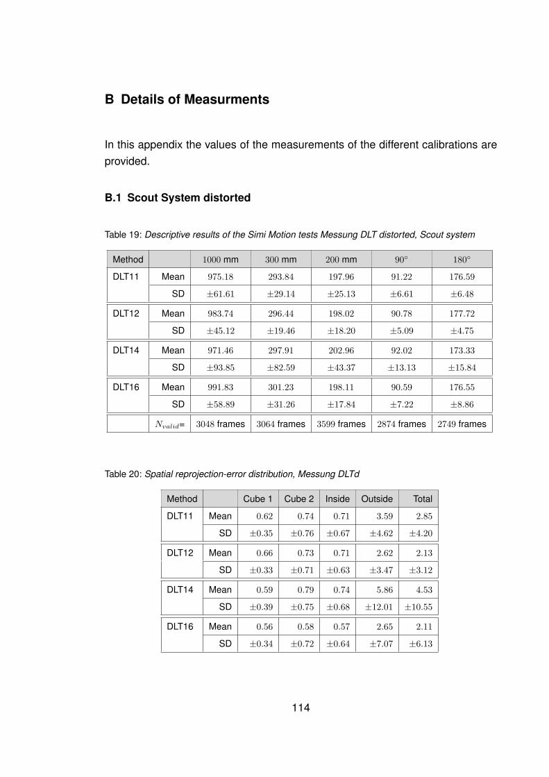
B Details of Measurments

In this appendix the values of the measurements of the different calibrations areprovided.

B.1 Scout System distorted

Table 19: Descriptive results of the Simi Motion tests Messung DLT distorted, Scout system

Method 1000 mm 300 mm 200 mm 90◦ 180◦

DLT11 Mean 975.18 293.84 197.96 91.22 176.59

SD ±61.61 ±29.14 ±25.13 ±6.61 ±6.48

DLT12 Mean 983.74 296.44 198.02 90.78 177.72

SD ±45.12 ±19.46 ±18.20 ±5.09 ±4.75

DLT14 Mean 971.46 297.91 202.96 92.02 173.33

SD ±93.85 ±82.59 ±43.37 ±13.13 ±15.84

DLT16 Mean 991.83 301.23 198.11 90.59 176.55

SD ±58.89 ±31.26 ±17.84 ±7.22 ±8.86


Table 20: Spatial reprojection-error distribution, Messung DLTd

Method Cube 1 Cube 2 Inside Outside Total

DLT11 Mean 0.62 0.74 0.71 3.59 2.85

SD ±0.35 ±0.76 ±0.67 ±4.62 ±4.20

DLT12 Mean 0.66 0.73 0.71 2.62 2.13

SD ±0.33 ±0.71 ±0.63 ±3.47 ±3.12

DLT14 Mean 0.59 0.79 0.74 5.86 4.53

SD ±0.39 ±0.75 ±0.68 ±12.01 ±10.55

DLT16 Mean 0.56 0.58 0.57 2.65 2.11

SD ±0.34 ±0.72 ±0.64 ±7.07 ±6.13

114


Table 21: Descriptive results of the Simi Motion tests Messung M15d, Scout system

Method 1000 mm 300 mm 200 mm 90◦ 180◦

2 Cam Mean 997.57 299.70 197.98 91.42 177.55

Nt = 3340 SD ±51.04 ±21.81 ±17.68 ±5.09 ±4.97

3 Cam Mean 985.87 297.32 196.98 91.25 177.25

Nt = 2756 SD ±56.32 ±25.28 ±16.96 ±5.54 ±5.48

4 Cam Mean 988.94 297.07 197.87 91.39 177.47

Nt = 2253 SD ±54.02 ±22.77 ±18.76 ±5.42 ±5.01

5 Cam Mean 977.56 293.71 197.06 91.50 177.40

Nt = 1471 SD ±58.92 ±23.86 ±21.09 ±5.81 ±5.11

6 Cam Mean 977.65 293.28 197.36 91.20 177.30

Nt = 519 SD ±63.92 ±25.56 ±22.70 ±6.11 ±5.38


Table 22: Spatial reprojection-error distribution, Messung 15d


2 Cam Mean 0.80 0.81 0.81 2.44 2.02

SD ±0.39 ±0.74 ±0.66 ±3.29 ±2.94

3 Cam Mean 1.26 0.93 1.02 2.76 2.31

SD ±0.57 ±0.77 ±0.73 ±3.82 ±3.40

4 Cam Mean 0.73 0.72 0.72 2.57 2.09

SD ±0.33 ±0.71 ±0.63 ±3.48 ±3.11

5 Cam Mean 0.59 0.68 0.65 2.77 2.21

SD ±0.30 ±0.72 ±0.64 ±3.80 ±3.41

6 Cam Mean 0.49 0.74 0.68 2.89 2.30

SD ±0.28 ±0.75 ±0.67 ±3.66 ±3.31

115



Method 1000 mm 300 mm 200 mm 90◦ 180◦

2 Cam Mean 967.33 290.49 191.71 91.13 177.34

Nt = 3356 SD ±68.37 ±26.96 ±24.93 ±6.45 ±5.82

3 Cam Mean 980.78 294.75 197.11 90.96 177.37

Nt = 2807 SD ±53.78 ±22.17 ±23.07 ±5.63 ±5.39

4 Cam Mean 978.15 294.38 196.38 90.98 177.36

Nt = 1903 SD ±53.93 ±22.29 ±21.85 ±5.54 ±5.34

5 Cam Mean 962.52 290.42 191.98 91.24 177.28

Nt = 876 SD ±67.46 ±26.16 ±21.93 ±6.27 ±5.72

6 Cam Mean 957.86 291.15 192.55 91.43 177.11

Nt = 187 SD ±76.19 ±29.87 ±21.06 ±6.72 ±6.22




2 Cam Mean 0.88 0.89 0.89 2.47 2.06

SD ±0.40 ±0.73 ±0.67 ±2.86 ±2.58

3 Cam Mean 0.80 0.84 0.83 2.49 2.06

SD ±0.40 ±0.71 ±0.65 ±3.00 ±2.70

4 Cam Mean 0.77 0.80 0.79 2.52 2.07

SD ±0.42 ±0.72 ±0.65 ±3.04 ±2.74

5 Cam Mean 0.84 0.89 0.88 2.68 2.20

SD ±0.47 ±0.82 ±0.75 ±3.26 ±2.93

6 Cam Mean 1.17 1.27 1.25 3.13 2.63

SD ±0.75 ±1.12 ±1.04 ±3.72 ±3.34

116



Method 1000 mm 300 mm 200 mm 90◦ 180◦

2 Cam Mean 1001.68 300.80 200.55 91.04 177.59

Nt = 3564 SD ±51.54 ±18.78 ±19.80 ±5.30 ±5.03

3 Cam Mean 999.40 300.34 201.02 91.09 177.49

Nt = 2692 SD ±57.23 ±21.22 ±21.16 ±5.62 ±5.30

4 Cam Mean 989.02 297.07 199.28 91.17 177.39

Nt = 1859 SD ±55.29 ±21.92 ±21.49 ±5.77 ±5.27

5 Cam Mean 981.26 295.48 198.26 91.07 177.33

Nt = 956 SD ±55.35 ±22.68 ±20.68 ±5.84 ±5.43

6 Cam Mean 979.83 294.88 198.21 90.83 177.20

Nt = 249 SD ±61.08 ±24.50 ±24.36 ±6.26 ±5.86




2 Cam Mean 1.20 1.13 1.15 2.28 1.99

SD ±0.46 ±0.80 ±0.72 ±2.57 ±2.30

3 Cam Mean 1.15 1.08 1.10 2.41 2.07

SD ±0.42 ±0.79 ±0.72 ±2.88 ±2.57

4 Cam Mean 0.97 0.93 0.94 2.57 2.15

SD ±0.47 ±0.81 ±0.74 ±3.23 ±2.90

5 Cam Mean 0.73 0.62 0.65 2.53 2.04

SD ±0.34 ±0.67 ±0.61 ±3.37 ±3.03

6 Cam Mean 0.78 0.74 0.75 2.74 2.22

SD ±0.45 ±0.80 ±0.72 ±3.65 ±3.28

117



Method 1000 mm 300 mm 200 mm 90◦ 180◦

2 Cam Mean 981.77 295.40 197.79 90.03 175.78

Nt = 1521 SD ±82.81 ±35.42 ±23.84 ±9.24 ±8.30

3 Cam Mean 982.62 296.42 198.67 89.89 176.01

Nt = 1075 SD ±77.21 ±29.90 ±24.28 ±8.81 ±8.23

4 Cam Mean 991.11 303.02 201.95 89.49 175.37

Nt = 629 SD ±116.98 ±54.11 ±52.14 ±9.61 ±9.20

5 Cam Mean 970.45 292.19 196.41 91.76 177.07

Nt = 324 SD ±47.40 ±26.33 ±19.92 ±6.43 ±5.59

6 Cam Mean 983.91 296.15 195.53 90.18 175.87

Nt = 96 SD ±74.53 ±33.20 ±27.95 ±8.96 ±7.55




2 Cam Mean 1.23 1.76 1.61 5.26 4.35

SD ±0.64 ±1.31 ±1.19 ±7.25 ±6.50

3 Cam Mean 0.89 1.36 1.23 4.49 3.68

SD ±0.46 ±1.09 ±0.98 ±6.30 ±5.66

4 Cam Mean 2.20 2.62 2.52 5.99 5.10

SD ±1.17 ±1.88 ±1.75 ±6.96 ±6.26

5 Cam Mean 0.52 0.78 0.71 3.15 2.52

SD ±0.29 ±0.80 ±0.71 ±4.60 ±4.11

6 Cam Mean 3.23 3.46 3.39 5.09 4.68

SD ±2.43 ±2.69 ±2.61 ±5.44 ±4.96

118


B.2 Scout system undistorted

Table 29: Descriptive results of the Simi Motion tests Messung DLT distorted, Scout system

Method 1000 mm 300 mm 200 mm 90◦ 180◦

DLT11 Mean 1000.56 301.20 198.94 89.77 179.19

SD ±10.93 ±5.23 ±3.35 ±0.82 ±1.12

DLT12 Mean 1000.30 301.33 198.84 89.80 179.11

SD ±12.56 ±5.87 ±3.94 ±1.15 ±1.26

DLT14 Mean 1019.04 316.85 205.28 89.73 174.62

SD ±101.94 ±80.84 ±37.74 ±7.22 ±15.84

DLT16 Mean 1017.17 316.97 206.63 89.60 174.25

SD ±106.77 ±81.96 ±39.10 ±7.34 ±17.19


Table 30: Spatial reprojection-error distribution, Messung DLTun

Method Cube 1 Cube 2 Inside Outside total

DLT11 Mean 0.45 0.50 0.49 0.61 0.58

SD ±0.24 ±0.25 ±0.25 ±0.49 ±0.45

DLT12 Mean 0.46 0.51 0.50 0.71 0.65

SD ±0.24 ±0.28 ±0.27 ±0.64 ±0.58

DLT14 Mean 0.52 0.56 0.55 3.00 2.36

SD ±0.28 ±0.41 ±0.38 ±9.94 ±8.56

DLT16 Mean 0.53 0.56 0.55 3.23 2.53

SD ±0.32 ±0.36 ±0.35 ±10.16 ±8.76

119


Table 31: Descriptive results of the Simi Motion tests Messung M15un, Scout system

Method 1000 mm 300 mm 200 mm 90◦ 180◦

2 Cam Mean 999.96 300.62 199.12 89.65 179.30

Nt = 3337 SD ±2.17 ±4.68 ±1.52 ±0.38 ±1.37

3 Cam Mean 999.93 300.62 199.13 89.65 179.30

Nt = 2715 SD ±2.30 ±4.69 ±1.54 ±0.39 ±1.37

4 Cam Mean 999.96 300.63 199.13 89.65 179.30

Nt = 2067 SD ±2.42 ±4.70 ±1.55 ±0.39 ±1.37

5 Cam Mean 999.87 300.62 199.09 89.65 179.28

Nt = 1316 SD ±2.79 ±4.73 ±1.59 ±0.41 ±1.37

6 Cam Mean 999.82 300.58 199.10 89.64 179.25

Nt = 618 SD ±3.24 ±4.84 ±1.76 ±0.45 ±1.38


Table 32: Spatial reprojection-error distribution, Messung 15un


2 Cam Mean 0.18 0.21 0.20 0.27 0.25

SD ±0.18 ±0.19 ±0.19 ±0.32 ±0.29

3 Cam Mean 0.18 0.21 0.20 0.28 0.26

SD ±0.18 ±0.219 ±0.19 ±0.33 ±0.30

4 Cam Mean 0.18 0.21 0.20 0.28 0.26

SD ±0.18 ±0.19 ±0.19 ±0.33 ±0.30

5 Cam Mean 0.19 0.21 0.21 0.31 0.28

SD ±0.18 ±0.19 ±0.19 ±0.34 ±0.32

6 Cam Mean 0.19 0.21 0.21 0.36 0.32

SD ±0.18 ±0.18 ±0.19 ±0.41 ±0.37

120


Table 33: Descriptive results of the Simi Motion tests Messung M16u, Scout system

Method 1000 mm 300 mm 200 mm 90◦ 180◦

2 Cam Mean 999.52 300.43 199.07 89.66 179.30

Nt = 3511 SD ±2.04 ±4.66 ±1.47 ±0.38 ±1.37

3 Cam Mean 999.39 300.42 199.08 89.66 179.30

Nt = 2827 SD ±2.12 ±4.66 ±1.47 ±0.38 ±1.37

4 Cam Mean 999.33 300.39 199.06 89.66 179.30

Nt = 2105 SD ±2.14 ±4.67 ±1.49 ±0.39 ±1.37

5 Cam Mean 999.47 300.41 199.08 89.66 179.30

Nt = 1331 SD ±2.43 ±4.71 ±1.52 ±0.40 ±1.37

6 Cam Mean 1000.65 300.34 199.09 89.65 179.09

Nt = 583 SD ±7.73 ±5.83 ±3.48 ±0.81 ±1.58




2 Cam Mean 0.17 0.20 0.19 0.25 0.24

SD ±0.18 ±0.19 ±0.19 ±0.30 ±0.28

3 Cam Mean 0.17 0.20 0.19 0.26 0.24

SD ±0.18 ±0.20 ±0.19 ±0.30 ±0.28

4 Cam Mean 0.17 0.20 0.19 0.27 0.25

SD ±0.18 ±0.20 ±0.19 ±0.31 ±0.29

5 Cam Mean 0.17 0.20 0.19 0.27 0.25

SD ±0.18 ±0.20 ±0.19 ±0.33 ±0.30

6 Cam Mean 0.18 0.23 0.22 0.49 0.42

SD ±0.18 ±0.21 ±0.21 ±0.53 ±0.48

121



Method 1000 mm 300 mm 200 mm 90◦ 180◦

2 Cam Mean 1001.91 300.08 200.02 89.15 178.38

Nt = 2424 SD ±25.10 ±14.17 ±12.03 ±2.17 ±2.73

3 Cam Mean 998.56 298.97 200.86 89.63 178.27

Nt = 1711 SD ±36.34 ±17.04 ±13.93 ±3.34 ±2.97

4 Cam Mean 1000.56 300.58 199.39 89.64 179.25

Nt = 1269 SD ±3.41 ±4.86 ±2.03 ±0.51 ±1.37

5 Cam Mean 999.60 300.28 199.08 89.64 179.24

Nt = 820 SD ±3.78 ±4.85 ±2.08 ±0.53 ±1.38

6 Cam Mean 1000.37 300.47 199.35 89.61 179.19

Nt = 364 SD ±5.64 ±5.22 ±2.44 ±0.63 ±1.40




2 Cam Mean 0.44 0.92 0.78 2.08 1.74

SD ±0.44 ±1.00 ±0.90 ±4.51 ±3.93

3 Cam Mean 0.47 1.01 0.86 2.31 1.93

SD ±0.46 ±1.10 ±0.99 ±4.97 ±4.34

4 Cam Mean 0.18 0.21 0.20 0.29 0.27

SD ±0.19 ±0.19 ±0.19 ±0.31 ±0.28

5 Cam Mean 0.18 0.21 0.21 0.31 0.28

SD ±0.19 ±0.19 ±0.19 ±0.32 ±0.29

6 Cam Mean 0.19 0.23 0.22 0.39 0.34

SD ±0.19 ±0.20 ±0.20 ±0.34 ±0.32

122



Method 1000 mm 300 mm 200 mm 90◦ 180◦

2 Cam Mean 1000.62 300.72 199.32 89.64 179.30

Nt = 3264 SD ±3.12 ±4.74 ±1.57 ±0.43 ±1.37

3 Cam Mean 1000.91 300.81 199.39 89.64 179.30

Nt = 2585 SD ±3.31 ±4.67 ±1.59 ±0.43 ±1.37

4 Cam Mean 1000.58 300.71 199.31 89.65 179.30

Nt = 1876 SD ±3.03 ±4.73 ±1.56 ±0.42 ±1.37

5 Cam Mean 1000.10 300.55 199.10 89.65 179.29

Nt = 953 SD ±3.42 ±4.78 ±1.62 ±0.46 ±1.37

6 Cam Mean 999.61 300.42 198.97 89.68 179.30

Nt = 163 SD ±3.99 ±4.70 ±1.81 ±0.49 ±1.37




2 Cam Mean 0.17 0.19 0.18 0.26 0.24

SD ±0.19 ±0.19 ±0.19 ±0.30 ±0.28

3 Cam Mean 0.17 0.19 0.18 0.26 0.24

SD ±0.19 ±0.19 ±0.19 ±0.30 ±0.28

4 Cam Mean 0.17 0.19 0.18 0.26 0.24

SD ±0.19 ±0.19 ±0.19 ±0.30 ±0.28

5 Cam Mean 0.17 0.19 0.19 0.28 0.25

SD ±0.19 ±0.19 ±0.19 ±0.31 ±0.28

6 Cam Mean 0.17 0.19 0.18 0.26 0.24

SD ±0.18 ±0.19 ±0.19 ±0.31 ±0.29

123



Method 1000 mm 300 mm 200 mm 90◦ 180◦

2 Cam Mean 1000.27 300.63 199.16 89.64 179.30

Nt = 3849 SD ±2.02 ±4.67 ±1.53 ±0.39 ±1.37

3 Cam Mean 1000.24 300.62 199.17 89.64 179.30

Nt = 2989 SD ±2.12 ±4.68 ±1.54 ±0.39 ±1.37

4 Cam Mean 1000.16 300.60 199.16 89.63 179.30

Nt = 2301 SD ±2.29 ±4.69 ±1.54 ±0.39 ±1.37

5 Cam Mean 1000.04 300.66 199.14 89.55 179.28

Nt = 1567 SD ±4.32 ±4.90 ±1.68 ±0.41 ±1.37

6 Cam Mean 1000.93 300.93 199.27 89.55 179.27

Nt = 702 SD ±7.19 ±5.33 ±2.04 ±0.49 ±1.37




2 Cam Mean 0.18 0.20 0.20 0.23 0.22

SD ±0.19 ±0.20 ±0.19 ±0.27 ±0.25

3 Cam Mean 0.18 0.20 0.20 0.23 0.22

SD ±0.19 ±0.05 ±0.19 ±0.27 ±0.25

4 Cam Mean 0.18 0.20 0.19 0.24 0.23

SD ±0.19 ±0.19 ±0.19 ±0.28 ±0.26

5 Cam Mean 0.18 0.20 0.19 0.27 0.25

SD ±0.19 ±0.19 ±0.19 ±0.30 ±0.27

6 Cam Mean 0.17 0.20 0.19 0.31 0.28

SD ±0.19 ±0.20 ±0.19 ±0.34 ±0.31

124



Method 1000 mm 300 mm 200 mm 90◦ 180◦

2 Cam Mean 1002.15 301.12 199.54 89.66 179.29

Nt = 2546 SD ±3.39 ±4.81 ±1.76 ±0.46 ±1.37

3 Cam Mean 1001.83 301.04 199.52 89.66 179.29

Nt = 1916 SD ±3.39 ±4.81 ±1.74 ±0.46 ±1.37

4 Cam Mean 1001.82 301.03 199.53 89.66 179.28

Nt = 1670 SD ±3.48 ±4.82 ±1.75 ±0.47 ±1.37

5 Cam Mean 1000.69 300.73 199.32 89.66 179.28

Nt = 852 SD ±3.29 ±4.78 ±1.68 ±0.46 ±1.37

6 Cam Mean 1000.65 300.71 199.44 89.66 179.27

Nt = 307 SD ±3.71 ±4.81 ±1.66 ±0.50 ±1.37




2 Cam Mean 0.21 0.22 0.22 0.26 0.25

SD ±0.19 ±0.19 ±0.19 ±0.29 ±0.27

3 Cam Mean 0.20 0.22 0.22 0.26 0.25

SD ±0.19 ±0.19 ±0.19 ±0.29 ±0.27

4 Cam Mean 0.20 0.22 0.21 0.26 0.25

SD ±0.19 ±0.12 ±0.19 ±0.29 ±0.27

5 Cam Mean 0.19 0.21 0.21 0.28 0.26

SD ±0.19 ±0.19 ±0.19 ±0.30 ±0.28

6 Cam Mean 0.18 0.19 0.19 0.28 0.26

SD ±0.19 ±0.19 ±0.19 ±0.31 ±0.28

125



Method 1000 mm 300 mm 200 mm 90◦ 180◦

2 Cam Mean 1001.75 301.10 199.56 89.62 179.28

Nt = 3621 SD ±3.45 ±4.79 ±1.65 ±0.44 ±1.37

3 Cam Mean 1001.71 301.10 199.55 89.62 179.29

Nt = 3193 SD ±3.33 ±4.78 ±1.64 ±0.44 ±1.37

4 Cam Mean 1001.53 301.05 199.50 89.62 179.29

Nt = 2851 SD ±3.16 ±4.77 ±1.63 ±0.43 ±1.37

5 Cam Mean 1001.44 301.02 199.48 89.62 179.29

Nt = 2381 SD ±3.01 ±4.75 ±1.61 ±0.42 ±1.37

6 Cam Mean 1001.28 300.99 199.46 89.63 179.30

Nt = 1496 SD ±2.91 ±4.74 ±1.56 ±0.42 ±1.37




2 Cam Mean 0.17 0.19 0.18 0.27 0.25

SD ±0.18 ±0.19 ±0.19 ±0.30 ±0.28

3 Cam Mean 0.16 0.19 0.18 0.27 0.25

SD ±0.18 ±0.19 ±0.19 ±0.30 ±0.28

4 Cam Mean 0.16 0.19 0.18 0.27 0.25

SD ±0.18 ±0.19 ±0.19 ±0.30 ±0.28

5 Cam Mean 0.16 0.19 0.18 0.27 0.25

SD ±0.18 ±0.19 ±0.19 ±0.30 ±0.28

6 Cam Mean 0.16 0.18 0.18 0.27 0.25

SD ±0.18 ±0.19 ±0.19 ±0.30 ±0.28

126



Method 1000 mm 300 mm 200 mm 90◦ 180◦

2 Cam Mean 1000.99 300.85 199.27 89.63 179.30

Nt = 2507 SD ±1.87 ±4.67 ±1.46 ±0.38 ±1.36

3 Cam Mean 1000.96 300.82 199.26 89.63 179.30

Nt = 1725 SD ±1.94 ±4.68 ±1.48 ±0.38 ±1.36

4 Cam Mean 1001.03 300.85 199.24 89.63 179.30

Nt = 1153 SD ±2.00 ±4.69 ±1.49 ±0.38 ±1.36

5 Cam Mean 1000.82 300.78 199.21 89.65 179.30

Nt = 568 SD ±2.19 ±4.69 ±1.53 ±0.39 ±1.37

6 Cam Mean 1000.89 300.81 199.34 89.65 179.28

Nt = 213 SD ±2.78 ±4.77 ±1.61 ±0.41 ±1.37




2 Cam Mean 0.19 0.22 0.21 0.23 0.22

SD ±0.19 ±0.20 ±0.20 ±0.26 ±0.24

3 Cam Mean 0.19 0.22 0.21 0.23 0.22

SD ±0.19 ±0.20 ±0.19 ±0.26 ±0.24

4 Cam Mean 0.19 0.21 0.21 0.23 0.22

SD ±0.19 ±0.20 ±0.19 ±0.26 ±0.24

5 Cam Mean 0.18 0.20 0.20 0.25 0.24

SD ±0.18 ±0.20 ±0.19 ±0.28 ±0.26

6 Cam Mean 0.19 0.21 0.20 0.28 0.26

SD ±0.18 ±0.20 ±0.20 ±0.30 ±0.27

127



Method 1000 mm 300 mm 200 mm 90◦ 180◦

2 Cam Mean 1000.57 300.73 199.31 89.66 179.30

Nt = 3337 SD ±2.16 ±4.65 ±1.48 ±0.39 ±1.37

3 Cam Mean 1000.54 300.73 199.31 89.65 179.30

Nt = 2715 SD ±2.18 ±4.66 ±1.49 ±0.39 ±1.37

4 Cam Mean 1000.54 300.73 199.32 89.65 179.30

Nt = 2067 SD ±2.24 ±4.67 ±1.49 ±0.39 ±1.37

5 Cam Mean 1000.43 300.72 199.30 89.65 179.30

Nt = 1316 SD ±2.33 ±4.67 ±1.48 ±0.39 ±1.37

6 Cam Mean 1000.40 300.75 199.30 89.65 179.30

Nt = 3337 SD ±2.44 ±4.68 ±1.51 ±0.39 ±1.37




2 Cam Mean 0.17 0.19 0.18 0.25 0.23

SD ±0.18 ±0.19 ±0.19 ±0.31 ±0.28

3 Cam Mean 0.17 0.19 0.18 0.25 0.23

SD ±0.18 ±0.19 ±0.19 ±0.31 ±0.28

4 Cam Mean 0.17 0.19 0.18 0.25 0.24

SD ±0.18 ±0.19 ±0.19 ±0.31 ±0.28

5 Cam Mean 0.17 0.19 0.18 0.27 0.24

SD ±0.18 ±0.19 ±0.19 ±0.31 ±0.29

6 Cam Mean 0.17 0.19 0.19 0.30 0.27

SD ±0.18 ±0.20 ±0.19 ±0.34 ±0.31

128



Method 1000 mm 300 mm 200 mm 90◦ 180◦

2 Cam Mean 1000.84 300.80 199.30 89.66 179.30

Nt = 2141 SD ±2.24 ±4.68 ±1.47 ±0.39 ±1.37

3 Cam Mean 1000.83 300.78 199.31 89.65 179.29

Nt = 1589 SD ±2.30 ±4.69 ±1.48 ±0.39 ±1.46

4 Cam Mean 1000.38 300.66 199.27 89.66 179.28

Nt = 957 SD ±2.58 ±4.72 ±1.55 ±0.40 ±1.37

5 Cam Mean 1000.60 300.76 199.30 89.66 179.25

Nt = 565 SD ±3.51 ±4.89 ±1.69 ±0.45 ±1.37

6 Cam Mean 1000.34 300.67 199.28 89.65 179.27

Nt = 151 SD ±3.02 ±4.78 ±1.62 ±0.42 ±1.37




2 Cam Mean 0.17 0.19 0.19 0.26 0.24

SD ±0.18 ±0.20 ±0.19 ±0.32 ±0.29

3 Cam Mean 0.17 0.20 0.19 0.26 0.24

SD ±0.18 ±0.19 ±0.19 ±0.32 ±0.29

4 Cam Mean 0.17 0.20 0.19 0.27 0.25

SD ±0.18 ±0.20 ±0.19 ±0.32 ±0.29

5 Cam Mean 0.17 0.20 0.19 0.29 0.27

SD ±0.18 ±0.20 ±0.19 ±0.32 ±0.30

6 Cam Mean 0.17 0.21 0.20 0.34 0.30

SD ±0.17 ±0.20 ±0.20 ±0.37 ±0.34

129


B.3 Baumer System

Table 51: Descriptive results of Measured values with DLT calibratoin (Messung 4) distorted, HDsystem

Method 1001 mm 301 mm 200 mm 90◦ 180◦

DLT11 Mean 990.88 299.35 199.99 89.75 178.31

SD ±20.64 ±12.15 ±4.31 ±1.65 ±1.83

DLT12 Mean 995.70 299.79 199.25 89.69 179.26

SD ±8.62 ±4.66 ±2.14 ±0.95 ±0.83

DLT14 Mean 997.60 301.24 199.62 89.87 177.4

SD ±28.87 ±25.80 ±7.46 ±2.45 ±6.23

DLT16 Mean 995.49 299.81 199.07 89.65 179.03

SD ±12.31 ±6.72 ±2.75 ±1.10 ±1.13


Table 52: Spatial reprojection-error distribution, Messung 4 distorted


SD ±1.80 ±5.01 ±4.74 ±8.61 ±7.55

DLT12 Mean 2.19 2.91 2.80 4.60 3.86

SD ±1.23 ±2.30 ±2.18 ±3.70 ±3.29

DLT14 Mean 2.30 3.61 3.41 12.06 8.53

SD ±1.33 ±5.39 ±5.01 ±28.31 ±22.41

DLT16 Mean 2.03 2.87 2.74 4.57 3.82

SD ±1.17 ±2.35 ±2.23 ±3.95 ±3.47

130


Table 53: Descriptive results of Measured values with calibration setup wandlength = 603 mm(Messung 4) distorted, HD system

Method 1001 mm 301 mm 200 mm 90◦ 180◦

2 Cam Mean 998.98 301.97 201.36 89.70 178.78

Nt = 1284 SD ±21.55 ±8.93 ±3.96 ±1.56 ±1.19

3 Cam Mean 998.73 301.91 201.31 89.71 178.78

Nt = 1206 SD ±21.69 ±8.90 ±3.98 ±1.57 ±1.19

4 Cam Mean 998.23 301.75 201.17 89.71 178.78

Nt = 1063 SD ±22.01 ±8.84 ±3.96 ±1.58 ±1.19

5 Cam Mean 997.39 301.53 200.96 89.71 178.77

Nt = 911 SD ±22.14 ±8.95 ±3.89 ±1.58 ±1.21

6 Cam Mean 993.09 300.21 200.17 89.72 178.72

Nt = 638 SD ±23.49 ±9.25 ±3.80 ±1.60 ±1.26

7 Cam Mean 986.03 298.17 198.68 89.76 178.68

Nt = 379 SD ±33.10 ±10.84 ±4.29 ±1.97 ±1.33

8 Cam Mean 969.23 294.60 193.79 90.33 177.93

Nt = 124 SD ±59.55 ±17.40 ±8.75 ±4.26 ±2.01


Table 54: Spatial reprojection-error distribution, Messung 4 distorted, 603 Wand

Method Cube 1 Cube 2 Inside Outside Total2 Cam Mean 2.83 3.49 3.39 6.60 5.34

SD ±1.99 ±2.79 ±2.70 ±5.90 ±5.14

3 Cam Mean 2.82 3.49 3.39 6.59 5.34

SD ±2.00 ±2.78 ±2.69 ±5.90 ±5.14

4 Cam Mean 2.80 3.46 3.36 6.57 5.31

SD ±2.00 ±2.79 ±2.69 ±5.89 ±5.14

5 Cam Mean 2.76 3.42 3.33 6.58 5.30

SD ±1.98 ±2.81 ±2.72 ±5.90 ±5.16

6 Cam Mean 2.64 3.43 3.32 6.84 5.42

SD ±1.90 ±3.05 ±2.93 ±6.23 ±5.45

7 Cam Mean 2.60 3.67 3.51 7.20 5.72

SD ±1.96 ±3.54 ±3.37 ±6.85 ±6.00

8 Cam Mean 21.94 22.32 22.27 26.22 24.62

SD ±26.10 ±26.74 ±26.65 ±26.37 ±26.55

131


Table 55: Descriptive results of Measured values with calibration setup wandlength = 1001 mm(Messung 4) distorted, HD system

Method 1001 mm 301 mm 200 mm 90◦ 180◦

2 Cam Mean 999.00 301.40 201.56 89.74 178.84

Nt = 1266 SD ±13.06 ±8.37 ±4.41 ±1.74 ±1.10

3 Cam Mean 998.63 301.31 201.53 89.74 178.84

Nt = 1144 SD ±13.26 ±8.33 ±8.33 ±1.76 ±1.10

4 Cam Mean 998.05 301.31 201.50 89.78 178.83

Nt = 905 SD ±13.70 ±8.39 ±4.50 ±1.80 ±1.11

5 Cam Mean 996.44 300.99 201.22 89.81 178.82

Nt = 701 SD ±14.08 ±8.47 ±4.46 ±1.79 ±1.12

6 Cam Mean 994.20 300.45 200.70 89.85 178.79

Nt = 517 SD ±14.51 ±8.74 ±4.38 ±1.74 ±1.17

7 Cam Mean 990.48 299.31 199.82 89.87 178.78

Nt = 300 SD ±15.58 ±8.73 ±4.21 ±1.63 ±1.21

8 Cam Mean 987.79 298.66 199.13 89.95 178.76

Nt = 96 SD ±16.86 ±9.11 ±4.38 ±1.64 ±1.23


Table 56: Spatial reprojection-error distribution, Messung 4 distorted, 1001 Wand


SD ±1.94 ±2.85 ±2.73 ±4.89 ±4.28

3 Cam Mean 2.91 3.58 3.46 5.59 4.73

SD ±1.93 ±2.80 ±2.68 ±4.89 ±4.27

4 Cam Mean 2.89 3.50 3.40 5.55 4.68

SD ±1.95 ±2.80 ±2.68 ±4.89 ±4.27

5 Cam Mean 2.82 3.42 3.32 5.61 4.67

SD ±1.96 ±2.81 ±2.69 ±5.02 ±4.38

6 Cam Mean 2.74 3.44 3.32 5.73 4.74

SD ±1.95 ±2.96 ±2.83 ±5.20 ±4.54

7 Cam Mean 2.75 3.52 3.38 5.90 4.87

SD ±1.99 ±3.04 ±2.90 ±5.29 ±4.64

8 Cam Mean 2.51 3.19 3.07 6.35 4.95

SD ±1.78 ±2.84 ±2.70 ±5.54 ±4.83

132


Table 57: Descriptive results of Measured values with calibration setup wandlength = 603 mm(Messung 4) undistorted, HD system

Method 1001 mm 301 mm 200 mm 90◦ 180◦

DLT11 Mean 995.37 299.67 199.16 89.73 179.41

SD ±7.78 ±2.55 ±2.67 ±1.30 ±0.35

DLT12 Mean 995.80 299.60 199.08 89.72 179.40

SD ±7.57 ±3.40 ±2.82 ±1.37 ±0.48

DLT14 Mean 995.32 299.45 199.11 89.74 179.35

SD ±8.57 ±3.67 ±3.01 ±1.43 ±0.53

DLT16 Mean 993.49 299.58 198.88 89.82 179.32

SD ±12.96 ±3.50 ±3.19 ±1.46 ±0.67


Table 58: Spatial reprojection-error distribution, Messung 4 undistorted


SD ±1.05 ±1.37 ±1.33 ±2.01 ±1.78

DLT12 Mean 1.88 2.58 2.47 3.47 3.05

SD ±1.09 ±1.78 ±1.71 ±2.71 ±2.40

DLT14 Mean 1.90 2.75 2.62 3.73 3.27

SD ±1.07 ±1.93 ±1.85 ±3.04 ±2.67

DLT16 Mean 1.98 2.66 2.56 3.42 3.06

SD ±1.08 ±1.83 ±1.75 ±3.03 ±2.61

133


Table 59: Descriptive results of Measured values with calibration setup wandlength = 603 mm(Messung 4) UNdistorted, HD system

Method 1001 mm 301 mm 200 mm 90◦ 180◦

2 Cam Mean 1001.52 300.97 200.16 89.62 179.59

Nt = 1290 SD ±2.01 ±1.17 ±2.73 ±1.37 ±0.21

3 Cam Mean 1001.53 300.97 200.17 89.61 179.59

Nt = 1205 SD ±2.01 ±1.18 ±2.73 ±1.37 ±0.21

4 Cam Mean 1001.52 300.97 200.17 89.61 179.59

Nt = 1084 SD ±2.02 ±1.20 ±2.73 ±1.37 ±0.21

5 Cam Mean 1001.56 300.98 200.18 89.61 179.59

Nt = 897 SD ±2.01 ±1.22 ±2.72 ±1.37 ±0.21

6 Cam Mean 1001.61 300.99 200.19 89.61 179.59

Nt = 650 SD ±2.03 ±1.24 ±2.72 ±1.37 ±0.21

7 Cam Mean 1001.44 300.95 200.17 89.61 179.59

Nt = 407 SD ±2.13 ±1.34 ±2.72 ±1.37 ±0.21

8 Cam Mean 1001.33 300.97 200.12 89.62 179.59

Nt = 136 SD ±2.39 ±1.27 ±2.72 ±1.37 ±0.21


Table 60: Spatial reprojection-error distribution, Messung 4 undistorted, 603 Wand


SD ±0.98 ±1.13 ±1.10 ±1.16 ±1.16

3 Cam Mean 1.42 1.59 1.56 1.67 1.66

SD ±0.98 ±1.13 ±1.10 ±1.16 ±1.16

4 Cam Mean 1.42 1.59 1.56 1.67 1.66

SD ±0.98 ±1.13 ±1.10 ±1.16 ±1.16

5 Cam Mean 1.42 1.59 1.56 1.67 1.66

SD ±0.98 ±1.13 ±1.10 ±1.16 ±1.16

6 Cam Mean 1.43 1.59 1.56 1.67 1.66

SD ±0.99 ±1.13 ±1.10 ±1.17 ±1.16

7 Cam Mean 1.43 1.59 1.55 1.96 1.67

SD ±0.99 ±1.13 ±1.10 ±1.19 ±1.18

8 Cam Mean 1.39 1.57 1.53 1.69 1.67

SD ±0.92 ±1.13 ±1.09 ±1.19 ±1.18

134



Method 1001 mm 301 mm 200 mm 90◦ 180◦

2 Cam Mean 1000.41 300.63 199.92 89.60 179.59

Nt = 1159 SD ±1.88 ±1.15 ±2.71 ±1.36 ±0.20

3 Cam Mean 1000.42 300.63 199.92 89.60 179.59

Nt = 895 SD ±1.88 ±1.15 ±2.71 ±1.36 ±0.20

4 Cam Mean 1000.36 300.63 199.92 89.60 179.59

Nt = 628 SD ±1.81 ±1.14 ±2.71 ±1.36 ±0.20

5 Cam Mean 1000.24 300.61 199.91 89.60 179.59

Nt = 438 SD ±1.78 ±1.13 ±2.71 ±1.36 ±0.20

6 Cam Mean 1000.27 300.64 199.91 89.61 179.59

Nt = 238 SD ±1.79 ±1.13 ±2.71 ±1.36 ±0.20

7 Cam Mean 1000.48 300.75 199.96 89.63 179.59

Nt = 82 SD ±2.09 ±1.23 ±2.72 ±1.37 ±0.21

8 Cam Mean 962.69 289.15 190.49 89.35 179.57

Nt = 9 SD ±29.65 ±8.81 ±6.28 ±3.04 ±0.28




SD ±1.04 ±1.15 ±1.13 ±1.13 ±1.13

3 Cam Mean 1.47 1.63 1.59 1.66 1.65

SD ±1.03 ±1.15 ±1.13 ±1.13 ±1.13

4 Cam Mean 1.47 1.62 1.59 1.66 1.65

SD ±1.03 ±1.14 ±1.12 ±1.14 ±1.13

5 Cam Mean 1.47 1.62 1.59 1.67 1.66

SD ±1.03 ±1.14 ±1.12 ±1.15 ±1.14

6 Cam Mean 1.43 1.62 1.59 1.67 1.66

SD ±0.97 ±1.14 ±1.11 ±1.14 ±1.14

7 Cam Mean 1.44 1.62 1.58 1.68 1.66

SD ±0.95 ±1.13 ±1.10 ±1.14 ±1.14

8 Cam Mean 2.21 1.85 1.90 2.25 2.20

SD ±1.28 ±1.21 ±1.23 ±1.55 ±1.52

135



Method 1001 mm 301 mm 200 mm 90◦ 180◦

2 Cam Mean 1000.89 300.82 200.05 89.60 179.59

Nt = 1300 SD ±1.97 ±1.19 ±2.73 ±1.37 ±0.20

3 Cam Mean 1000.87 300.81 200.04 89.60 179.59

Nt = 1289 SD ±1.98 ±1.19 ±2.73 ±1.37 ±0.20

4 Cam Mean 1001.01 300.85 200.07 89.60 179.59

Nt = 1252 SD ±1.93 ±1.19 ±2.73 ±1.37 ±0.20

5 Cam Mean 1001.00 300.85 200.07 89.60 179.59

Nt = 1210 SD ±1.92 ±1.19 ±2.73 ±1.37 ±0.20

6 Cam Mean 1001.12 300.88 200.09 89.60 179.59

Nt = 1088 SD ±1.90 ±1.21 ±2.73 ±1.37 ±0.21

7 Cam Mean 1000.90 300.81 200.05 89.60 179.59

Nt = 847 SD ±2.02 ±1.26 ±2.73 ±1.37 ±0.21

8 Cam Mean 999.39 300.40 199.74 89.61 179.59

Nt = 413 SD ±3.40 ±1.51 ±2.78 ±1.04 ±0.21




SD ±0.97 ±1.11 ±1.08 ±1.11 ±1.11

3 Cam Mean 1.44 1.58 1.55 1.66 1.65

SD ±0.96 ±1.11 ±1.08 ±1.11 ±1.11

4 Cam Mean 1.44 1.58 1.55 1.66 1.65

SD ±0.97 ±1.11 ±1.08 ±1.11 ±1.11

5 Cam Mean 1.44 1.58 1.55 1.66 1.65

SD ±0.97 ±1.11 ±1.08 ±1.11 ±1.11

6 Cam Mean 1.45 1.58 1.55 1.66 1.65

SD ±0.98 ±1.11 ±1.09 ±1.12 ±1.11

7 Cam Mean 1.46 1.58 1.55 1.67 1.65

SD ±1.01 ±1.11 ±1.09 ±1.12 ±1.12

8 Cam Mean 1.51 1.58 1.56 1.68 1.66

SD ±1.09 ±1.10 ±1.10 ±1.13 ±1.12

136

C Data sheets

C.1 Pretest

137

5

H1212BH612A■Specifications12mm6mmFocal Length1:1.21:1.2Max. Aperture Ratio

F1.2～22F1.2～CloseIris RangeManualManualIris

OperationMethod ManualManualFocus

――――――――Zoom16.9332.97Horizontal1/4 Format

Angle of View 12.7024.84Vertical22.6043.55Horizontal1/3 Format

Angle of View 16.9332.97Vertical30.1856.93Horizontal1/2 Format

Angle of View 22.6043.55Vertical0.2m0.2mMin. Object Distance

13.87mm14.31mmBack Focal Length17.526mm17.526mmFlange Back Length

φ27mm P=0.5mmφ40.5mm P=0.5mmFilter Screw Size－20˚C～＋50˚C－20˚C～＋50˚CTemperature Rangeφ30×35.5mmφ42×46mmDimensions

67g125gWeightLock Screw ExtraLock Screw ExtraRemarks

■H612A(C60607) C-MOUNT Unit:mm

1 / 2 Format Manual Iris■H1212B(C61215) C-MOUNT Unit:mm

Image device Type 1/3 (diag. 5.92 mm) progressive scan, KODAK CCDEffective picture elements 648 (H) x 488 (V)Picture size 640 (H) x 480 (V) (all modes and color formats) Cell size 7.4 µm x 7.4 µmResolution depth 8 bit / 10 bit / 12 bit / 14 bit / 16 bit (High SNR mode)Lens mount C-Mount / CS-Mount Digital interface IEEE1394b, 2xbilingual(daisy chain) IEEE1394b, 1 x bilingual, 1 x GOF connector (2 x optical fiber on LCLC)Transfer rate 100 Mbit/s, 200 Mbit/s, 400 Mbit/s, 800 Mbit/sFrame rates Up to 208 fps (Mono8, Raw8), 139 fps (YUV 4:1:1), 105 fps (YUV 4:2:2, Raw16), 70 fps (RGB8)Gain control mono: Manual 0-22 dB, auto gain; color: Manual 0-20 dB, auto gainShutter speed 18 µs … ~ 67 s, auto shutter (select. AOI)

External trigger shutter Programmable, trigger level controlsingle trigger, bulk trigger, programmable trigger delay

Smart features AGC/AEC/AWB with autofunction AOI; only color: AWB/color correction/hue/saturation; real-timeshading correction, LUT, 64 MB image memory, mirror, binning (only b/w), sub-sampling, High SNR,

storable user sets, 2 progr. inputs, 4 progr. outputs, RS-232 port, SIS [secure image signature], sequence mode, anti-smear mode, 4x/8x binning, 12-bit speed increase mode

Power requirements DC 8 V bis 36 V (via IEEE 1394 cable or 12-pin HIROSE)Power consumption Typ. 5 watt (@ 12 V DC); fiber: Typ. 5.75 watt (@ 12 V DC)Dimensions 96.8 mm x 44 mm x 44 mm (L x W x H); incl. connectors, w/o tripod and lensMass 250 g (without lens)Operating temperature +5 … +50 ° Celsius housing temperature (without condensation)Storage temperature -10 … +60 ° Celsius ambient temperature (without condensation)Regulations EN 55022, EN 61000, EN 55024, FCC Class B, DIN ISO 9022 , RoHS (2002/95/EC)Options IR cut/pass filter (mono), protection glass (color), host adapter card, angled head,

power out (HIROSE), AVT FirePackage/Direct FirePackage/Fire4Linux

AOI height / pixel Frame rate / fps

480 208300 314 240 372150 551 120 640

60 94130 135810 1778

Pin Signal1 External GND2 External Power (8...36 V DC)3 GP Output 44 GP Input 1 (Default: Trigger)5 GP Output 3 (Default: Busy)6 GP Output 1 (Default: IntEna)7 GP Input GND8 RxD (RS-232)9 TxD (RS-232)10 GP Output Power(max. 35 V DC)11 GP Input 2 (CMOS/TTL)12 GP Output 2

ALLIED VISION TECHNOLOGIES GMBHTaschenweg 2a | D-07646 Stadtroda | GermanyPhone: +49 (0)36428 6770 | Fax: +49 (0)36428 677-24www.alliedvisiontec.com | [email protected]

AVT Cameras PIKE F-032B / F-032CPIKE F-032B / F-032C fiber

AVT PIKE F-032B / F-032CAVT PIKE F-032B / F-032C fiber

Design and specification of the described product(s)are subject to change without notice.© 08/2007

Camera SpecificationsS PIKE F-032 B/C PIKE F-032 B/C fiber

Copper / Daisy ChainCopper / GOF connections

Sensor specifications b/w; color (extracted from the data sheet of the sensor - excluding lens and filter)

Dimensions

3.4×

C-12

Applicable camera (model)

Unit : mm

Vari-Focal Wide Angle

High image-quality monitoring with optical performance supporting 3 megapixels. Compatible with a wide range - 1/2", 1/3" and 1/4" - cameras. Wide f3.8-13mm range accommodates various applications. Designed to maximize optical performance with high-accuracy aspheric lens, low-dispersion glass, and high refractive-index glass. Built-in ND filter of T360, supporting high sensitivity cameras.

●

●

●

●

●

FUJINON CCTV LENS

For SecurityVari-Focal DV3.4×3.8SA-SA1 1 1

42

3121

3

For Megapixel Camera

MEGA

PIXEL

VARI-F

OCAL

LENSES

Metal Mount

ND Filter

DC Auto Iris

Long Cable Aspherical Lens Wide Aperture Rate

Telephoto Long Focal

C Mount

RoHS Compliant

＊Photograph is a similar model.

IRIS CONTROL CABLE (CONNECTOR : 4-PIN PLUG)

+30 0100

DV3.4x3.8SA-

1:1.4/3.8-13mm

φ 48.8

14.8 11.8

φ 45.7

26.7

φ 19

φ 28

3.8

57

5.4（MAX.）

64.2（MAX.）

3.8～13（3.4×） F1.4 ～ T360（Equivalent to F360）

Manual Manual

Auto（DC Type） 97°34′ × 71°47′ 28°23′ × 21°18′ 71°47′ × 53°25′ 21°18′ × 15°59′ 53°15′ × 39°41′ 15°59′ × 11°59′ 107°12′ × 58°10′ 30°55′ × 17°25′ 78°34′ × 43°18′ 23°12′ × 13°04′ 58°10′ × 32°20′ 17°25′ × 9°48′ ∞ ～ 0.3 715 × 452 170 × 126 452 × 313 126 × 94 313 × 225 94 × 70 851 × 347 185 × 103 511 × 248 138 × 77 347 × 181 103 × 57 10.60 461 ― C 80

23mA（Max.） at DC 4V

Drive Coil Damping Coil

190Ω 500Ω

Focal Length （mm） Iris Range

Zoom Focus Iris

Operation

Focusing Range （From Front Of The Lens）（m）

Back Focal Distance （in air）（mm） Exit Pupil Position （From Image Plane）（mm）

Filter Thread （mm） Mount Mass （g）

Coil Resistance

Current Consumption

1/3"

1/4"

WIDE

TELE

WIDE

TELE

WIDE

TELE

1/3"

1/2"

1/2"

1/3"

1/4"

WIDE

TELE

WIDE

TELE

WIDE

TELE

1/2"

1/4"

WIDE

TELE

WIDE

TELE

WIDE

TELE

1/3"

1/2"

1/4"

WIDE

TELE

WIDE

TELE

WIDE

TELE

Angle Of View （H×V）

Object Dimensions at M.O.D.

（H×V）（mm）

Remarks

（*1）

Wiring

Open

TowardOpen

Lens

Drive Coil

Damping Coil

GREEN

BLUE

GRAY

WHITE

2

4

1

3

Connector4-PIN PLUG

［Lens Image］

3.8mm

13mm

Angle Of View （H×V）

Aspect Ratio 16：9

Object Dimensions at M.O.D.

（H×V）（mm） Aspect Ratio 16：9

・With Metal Mount （*1）When power is turned off, iris will 　　automatically close.DV3.4×3.8SA-SA1L：　　Long Cable Type（230mm）

Model No: LMZ69M Minimum object distance : 10mm ～　∞

Format size: 2/3” At Macro use : 10mm

Focal length: 11.5mm – 69mm (6x) At Close-up use : 500mm

Relative Aperture(F): 1: 1.4 At Standard use : 1000mm

Iris range: F1.4 – close

Angle of View (Horizontal x Vertical) Back Focal length: 17.93mm (in Air)

2/3” 41.9°x 32°( at f=11.5mm ) Flange back : 17.526mm (in Air)

7.3° x 5.5°( at f=69mm ) Locking screws: Zoom, Focus , Airis

FOV at Minimum object distance (Horizontal x Vertical): Operation Temperature: -10℃　~　+50℃

　　　　　　　　　　　　　　　　　　　　　　　　　　　　　　　 Mount: C-mount

2/3” f=11.5mm: FOV 72.8 x 54.6 cm Filter Diameter: 46mm x P0.75

f=11.5mm, close-up FOV 36.4 x 27.3cm Weight: 300g

2/3” f=69mm: FOV 12.8 x 9.6 cm

f=69mm, close-up FOV 6.4 x 4.8 cm

2/3” Macro FOV 3.2 x 2.4 cm

HXC40 Facts and DataDigital Monochrome Matrix Camera, 4 Megapixel, CameraLink®

Sensor InformationModel Name CMOSIS CMV-4000

Type 1“ progressive scan CMOS

Native Resolution 2048 ! 2048 pixels

Exposure Time 4 µsec ... 1 sec

Image Pre-processingAnalog Controls Offset (0 ... 255 LSB)

Color Modes Mono

Mechanical DataHousing Aluminum, IP40

Lens Mount C-Mount, F-Mount

Dimensions 52 ! 52 ! 37 mm

Weight 185 g

Electrical DataPower Supply 9.6 ... 30 V DC

Power Consumption approx. 5.5 Watts

Environmental DataOperating Temperature +5 °C ... +60 °C (+41 °F ... +131 °F)

Humidity 10% ... 90% non condensingBaumer Optronic GmbH Badstrasse 30DE-01454 Radeberg, GermanyPhone +49 (0)3528 4386 0Fax +49 (0)3528 4386 [email protected]/cameras

Tech

nica

l dat

a ha

s bee

n fu

lly c

heck

ed, b

ut a

ccur

acy

of p

rinte

d m

atte

r not

gua

rant

eed.

Su

bjec

t to

chan

ge w

ithou

t not

ice. P

rinte

d in

Ger

man

y 04

/11

Acquisition FormatsImage Formats Full Frame

Binning 2x1Subsampling 2x2

2048 ! 2048 pixels1024 ! 2048 pixels1024 ! 1024 pixels

max. 180.0 fps max. 180.0 fpsmax. 357.0 fps

Pixel Formats Mono8, Mono10, Mono12

Partial Scan True Partial Scan, Region of Interest (ROI) arbitrary

Camera FeaturesInternal Buffer 256 MBytes (max. 60 images)

Synchronization Free running, Trigger

Trigger Sources Hardware, Software, FrameGrabber

Trigger Delay 0 ... 2 sec, Tracking and buffering of up to 512 trigger signals

Digital I/Os 3 input lines (with Debouncer), 3 output lines

Interfaces and ConnectorsData Interface CameraLink® Base, Medium und Full

Connector: 2x Standard SDR26 (Mini CL)

Process Interface M8 / 8 pins

Power Interface M8 / 3 pins

SpecificationsProduct Type

Memory

Data Rates

Camera Link Compliance

EU Compliance

Laser Safety

Noise

Transceivers

Triggering / Serial

Cabling

Power

Physical

Environmental

System and Software

RCX C-Link is a remote camera extension adapter for

FIFOs for up to several lines of data; no frame memory

Wavelength Cable Range at 1.25 Gb/s Range at 2.5 Gb/s

Support ContactEngineering Design Team (EDT), Inc.

Ordering Options- Camera Link mode: Base

850

Switchcraft

110

- Environmental: Extended temperature

Bold Ask about custom options.

technische universität münchen department of sport and ...€¦ · department of sport and health...

Documents