Technische Universitat Berlin

Institut fur Mathematik

PDE-constrained control using ComsolMultiphysics – Control of the

Navier-Stokes equations

Thomas Slawiga

aTU Berlin, Institut f. Mathematik, Strasse des 17. Juni 136 MA 4-5, 10623Berlin, Germany, email: slawig@math.tu-berlin.de, phone: ++49 30 314 28035,fax: ++49 30 314 79706.

Technical Report 2005/26

Preprint-Reihe des Instituts fur MathematikTechnische Universitat Berlin

Report 2005/26 August 2006

PDE-constrained control using Comsol Multiphysics –

Control of the Navier-Stokes equations

Thomas Slawig∗

August 8, 2006

Abstract

We show how the software Comsol Multiphysics can be used to solve PDE-constrainedoptimal control problems. We give a general formulation for such kind of problems and derivethe adjoint equation and optimality system. Then these preliminaries are specified for thestationary Navier-Stokes equations with distributed and boundary control. The main stepsto define and solve a PDE with Comsol Multiphysics are described. We describe how theadjoint system can be implemented, and how the optimality system can be used by ComsolMultiphysics’s built-in functions. Special crucial topics concerning efficiency are discussed.Examples with distributed and boundary control for different type of cost functionals in 2and 3 space dimensions are presented.

Updated version for Comsol Multiphysics 3.2Comsol Multiphysics is a trademark of Comsol Inc.The original publication is available at www.springerlink.comKey words: Optimal control, finite element method, Navier-Stokes equationsAMS subject classification: 49K20, 65K10, 65N30, 35Q30, 76D05

1 Introduction

The effective numerical solution of PDE-constrained control problems requires expertise in severaldisciplines of applied mathematics: Knowledge in the theory of the underlying PDE (e.g. existenceand uniqueness results) has to be combined with the choice and analysis of an appropriate controlstrategy, specifically when adjoint-based algorithms are used. From the numerical point of view,effective discretization schemes and linear or nonlinear solvers for the state equation have to becombined with a suitable optimization method.

Any of these tasks alone may be rather challenging, even more when real-world applicationsare considered. In many cases, industrial problems are solved numerically by using commercialor legacy software. Its development has incorporated huge amounts of both work and knowledge,and thus it cannot be discarded when proceeding from the pure simulation to mathematical opti-mization and control. The alternative of plugging in the state equation solver in an off-the-shelveoptimization routine – the simplest way of the so-called ”first discretize then optimize” approach– is often not very successful, too.

A remedy would be to take advantage of the available state equation (PDE) solver, and combineit with a solver for the analytically derived adjoint equation. This solver has to be implemented.Even though the adjoint equation is always linear, the original PDE solver can not be used inmost cases, specifically if the state equation is nonlinear.

In this paper we show how this strategy can be implemented when using the commercialsoftware Comsol Multiphysics R©[2]. Somehow Comsol Multiphysics is a successor of the

∗TU Berlin, Institut f. Mathematik, Strasse des 17. Juni 136 MA 4-5, 10623 Berlin, Germany, email:slawig@math.tu-berlin.de, phone: ++49 30 314 28035, fax: ++49 30 314 79706.

1

PDE toolbox in Matlab R©[8], and it is also widely used in education and university research. Onthe other hand it offers many typical features of commercial solvers: A graphical user interface,geometry import functions and grid generators for 1,2, and 3 space dimensions, and post-processingfacilities. As Matlab, also Comsol Multiphysics is more and more used in real industrialapplication, at least according to the web site of the distributors. The chances that its applicationwill increase in the future are quite good, since Comsol Multiphysics offers a lot of predefinedequations and ”application modes” (for example for fluid and structural mechanics), variableFinite Element ansatz spaces, and state-of-the-art numerical algorithms for the solution of linearand non-linear systems.

Its main advantage, and the reason why we use Comsol Multiphysics here, is that it alsoallows a more mathematical equation-based modeling, i.e. the opportunity to define a PDE byits coefficients or even in weak form, and the chance to invoke commands it from the Matlabprompt. In this paper we show how these features can be used to design a complete controlframework that solves the optimality system of a PDE-constrained control problem as a coupledequation system by the built-in nonlinear solver. Due to the high-level functions provided by thesoftware, the complete control program or script is comparably short. The possibility to call thefunctions from the command line also allows the use of optimization routines written in Matlab.We show the structure of a control script for the cases of distributed and boundary control forthe stationary incompressible Navier-Stokes equations. Due to the general applicability of theComsol Multiphysics software it is possible to transfer the presented approach to other stateequations as well.

The structure of the paper is as follows: In the next section we continue with a generaldescription of PDE constrained control problems with distributed and boundary control. Wedescribe the form of the optimality system including the derivation of the adjoint equation. InSec. 6 we specialize these results for the test application that we used, the stationary Navier-Stokesequations (NSE). Then we present Comsol Multiphysics’s solution procedure for the NSE, anddescribe the basic data, PDE definition and solver structures, as far as they are important forour purpose. We show how the optimality system can be realized in Comsol Multiphysics.Afterwards we present efficient model scripts to solve the control problems. We emphasize thecrucial points to obtain a really flexible and effective framework that may be extended to otherstate equations as well. We end the paper by showing numerical results and a short summary.

2 PDE-constrained control problems

In this section we present the form of a general PDE-constrained control problem, including theadjoint equation, the optimality system, and a representation of the gradient of the cost. Thegeneral form can then be specialized for the given type of state equation. We emphasize thatthe following computations are formal, and thus for a mathematically correct setting furthertheoretical investigations are necessary. For details see e.g. [7].

The general form of a PDE-constrained control problem is the following. Let U, Y be Hilbertspaces. The aim is to minimize a functional

J : Y × U → R

under the constraint

e(y, u) = 0, e : Y × U → Z, (1)

where y ∈ Y denotes the state and u ∈ U the control. Clearly y thus depends on u and we willalso sometimes write y = y(u) and define J as J(u) := J(y(u), u). Additional constraints of theform y ∈ Yad ⊂ Y, u ∈ Uad ⊂ U (i.e. state and control constraints) may be given as well. Theconstraint (1) represents a PDE given on a domain Ω with corresponding boundary conditions.We consider only stationary problems here, otherwise there would be an initial condition, too.

2

A typical example for the cost J is the tracking type functional

J(y, u) =12

∫Ωc

|y − yd|2dx +α

2‖u‖2

U (2)

with regularization parameter α > 0. Here the control volume Ωc is a subset of the domain Ω. Thefunctional measures the distance between the solution y = y(u) of the state equation (1) to a giventarget or desired state yd. Moreover it takes into account the control cost by the regularizationterm. In a similar way one may consider a functional that measures this distance only on theboundary ∂Ω or a part of it. The state equation (1) consists of the PDE and boundary conditions,for distributed control u appears in the PDE, for boundary control in the boundary conditions.

2.1 Adjoint equations and optimality systems

In this subsection we show the general process to get the optimality system or a representation ofthe gradient of J . We introduce the Lagrange functional associated with the constrained problem

minu∈U

J(y, u) subject to (1). (3)

It is defined as

L : Y × U × Z∗, L(y, u, λ) := J(y, u) + 〈λ, e(y, u)〉Z∗,Z

where 〈·, ·〉Z∗,Z denotes the pairing between Z and its dual Z∗. Since in the case of a PDE-constrained problem e is vector-valued (at least due to boundary conditions) we have Z = Z1 ×. . .× Zn. Thus Z∗ is isometrically isomorph to the Cartesian product of the duals Z∗

i , i.e. Z∗ ∼=Z∗

1 × . . .× Z∗n, and the dual pairing is given as

〈λ, e(y, u)〉Z∗,Z =n∑

i=1

〈λi, ei(y, u)〉Z∗i ,Zi

.

The necessary optimality condition for saddle point of L and a minimum of (3) are then computedby setting the directional derivatives of L with respect to (y, u, λ) equal to zero in all admissibledirections. We get

Ly(y, u, λ)y = Jy(y, u)y + 〈λ, ey(y, u)y〉Z∗,Z = 0 ∀y ∈ YLu(y, u, λ)u = Ju(y, u)u + 〈λ, eu(y, u)u〉Z∗,Z = 0 ∀u ∈ ULλ(y, u, λ)λ = 〈λ, e(y, u)〉Z∗,Z = 0 ∀λ ∈ Z

(4)

where the subscript denotes the corresponding partial derivative. The first equation is called theadjoint equation, the second gives a relation between Lagrange multiplier z and the control u, andthe third one is just the state equation (1). The adjoint may also be written as

ey(y, u)∗λ = −Jy(y, u) in Z∗,

where A∗ denotes the adjoint operator of A. The optimality system (4) may be solved directly inthe so-called one-shot approach. Another alternative is to use a gradient-based iterative algorithmto solve (3). Then the directional derivative of J is needed. By the chain rule it is given as

J ′(u)u = Jy(y, u)y′(u)u + Ju(y, u)u.

In a similar way the total derivative of (1) with respect to u is

ey(y, u)y′(u)u + eu(y, u)u = 0 ∀u ∈ U.

Adding the duality pairing of this expression with the Lagrange multiplier λ gives

J ′(u)u = Jy(y, u)y′(u)u + 〈λ, ey(y, u)y′(u)u〉Z∗,Z

+Ju(y, u)u + 〈λ, eu(y, u)u〉Z∗,Z .

3

The first two terms equal zero due to the adjoint equation (with y = y′(u)u). Thus J ′ can becharacterized without explicitly knowing y′(u). After solution of both state and adjoint equation

J ′(u)u = Ju(y, u)u + 〈λ, eu(y, u)u〉Z∗,Z (5)

can be evaluated and used in an iterative optimization algorithm.

3 Application on the Navier-Stokes equations

Now we specialize the results of the last section for distributed and boundary control for thestationary NSE. The equations describe the flow of an incompressible Newtonian fluid in a domainΩ ⊂ Rd with d ∈ 2, 3. Unknowns are velocity vector v = (vi)d

i=1 and pressure p. Control problemfor the NSE are frequently studied, since they have a wide range of applications. Here we referto [6],[1],[4][10],[3]. For the theory and numerics of the equations themselves see [5] and [12]. Thestationary NSE read

−div (ν∇v) + v · ∇v +∇p = f + uD in Ω−div v = 0 in Ω

v = g on Σd

v = uB on Σc

ν∂ηv − pη = 0 on Σn

(6)

The first vector-valued equation represents the balance of momentum, the second one the balanceof mass in the fluid. Here f is a given volume force vector, ν the viscosity of the fluid or indimensionless form the inverse of the Reynolds number. The functions uD and uB are the controls.The gradient of v and the nonlinear convective term are defined as

∇v :=(∂vj

∂xi

)d

i,j=1, v · ∇w :=

( d∑j=1

vj∂wi

∂xj

)d

i=1.

Here the dot denotes the scalar product where the sum is taken over the two adjacent indices ofthe components of the operands. The boundary conditions are formulated in a general way with

• a part Σd with Dirichlet boundary conditions for the velocity. These may be inhomogeneouswhich refers to an prescribed in- or outflow, or homogeneous which refers to rigid walls witha no-slip condition.

• a part Σc with Dirichlet boundary conditions for the velocity, when this is used as control.This refers to blowing/sucking or applying a tangential force on the fluid. For distributedcontrol we set Σc = ∅.

• a part Σn with a natural boundary conditions. These are incorporated implicitly in the weakformulation, as we will show later. For the NSE this is a mixed condition for the normalderivative ∂η := η · ∇ of the velocity and the pressure. This condition represents a freeoutflow region and is sometimes also referred to as a ”do nothing” condition.

Here η denotes the outer normal vector on the boundary ∂Ω = Σd ∪ Σc ∪ Σn. The weak formof the equations is derived in the standard way. We do not include any homogeneous boundarycondition in the definition of the ansatz space which would also be possible, e.g. choose H0

1 (Ω)d

in the case ∂Ω = Σd and g = 0. We denote by V := H1(Ω)d the Sobolev space of vector-valuedfunctions with values and first derivatives in L2(Ω). As test space we use

W := w ∈ V = H1(Ω)d : w|Σd∪Σc = 0.

The pressure is uniquely defined in P := L2(Ω), except for Σn = ∅ where this is the case only in

P := L20(Ω) := p ∈ L2(Ω) :

∫Ω

pdx = 0,

4

which is isometrically isomorph to L2(Ω)/R. In computations uniqueness of the pressure is usuallyrealized by fixing the value to zero in one node. The velocity is unique only if ν is big enoughin relation to the norm of f , compare [5, Theorem IV.2.4]. The outflow condition is the naturalboundary condition when applying Green’s formula to the Laplace operator for v and the gradientof p, compare [5, I.(2.17),(2.18)]. Then we obtain the weak formulation: Find (v, p) ∈ V × P assolution of

ν(∇v,∇w)Ω + (v · ∇v, w)Ω − (p, div w)Ω − (f + uD, w)Ω = 0 ∀w ∈ W−(div v, q)Ω = 0 ∀q ∈ P

v − g = 0 on Σd

v − uB = 0 on Σc

(7)

Here (·, ·)Ω is the L2 inner product, where we do not distinguish in the notation between scalar-,vector-, and tensor- or matrix-valued functions. For vector-valued functions v, w we use (v, w)Ω :=∑d

i=1(vi, wi)Ω, for matrix-valued functions (v, w)Ω :=∑d

i,j=1(vij , wij)Ω.To fit the equations in the framework of the last section the two remaining boundary conditions

are formulated in weak form in L2(Σd)d and L2(Σc)d, respectively. Then (7) has the form (1)where e has four components. We thus get a Lagrange multiplier (λ1, λ2, λ3, λ4) ∈ Z∗ = (W ×P × L2(Σd)d × L2(Σc)d)∗ ∼= W × P × L2(Σd)d × L2(Σc)d. The fourth component is only neededfor boundary control. Note that P ∗ ∼= P in both cases.

3.1 Lagrange functional and adjoint equation

With y := (v, p) ∈ V × P =: Y, u := (uD, uB) the Lagrangian has the form

L(y, u, λ) = J(v, p, u) + ν(∇v,∇λ1)Ω + (v · ∇v, λ1)Ω − (p, div λ1)Ω−(f + uD, λ1)Ω − (div v, λ2)Ω + (v − g, λ3)Σd

+ (v − uB , λ4)Σc .

The adjoint system is obtained by computing the derivative in direction y = (w, q), compare thefirst equation in (4), as

ν(∇w,∇λ1)Ω + (v · ∇w + w · ∇v, λ1)Ω−(div w, λ2)Ω + (w, λ3)Σd

+ (w, λ4)Σc

= −Jv(v, p, u)w ∀w ∈ V

−(div λ1, q)Ω = −Jp(v, p, u)q ∀q ∈ P(8)

Using Green’s formula we obtain (with λ1 ∈ W and thus λ1|Σd∪Σc = 0):

ν(∇w,∇λ1)Ω = −(div(ν∇λ1), w)Ω + ν(∂ηλ1, w)Σn∪Σd∪Σc

−(div w, λ2)Ω = (∇λ2, w)Ω − (λ2η, w)Σn∪Σd∪Σc

(v · ∇w, λ1)Ω = −(v · ∇λ1, w)Ω + ((v · η)λ1, w)Σn

see [5, I.(2.17-18), Lemma IV.2.2] and [11, Lemma 6.3]. Moreover

(w · ∇v, λ1)Ω =∫

Ω

∑i,j

wj∂vi

∂xjλ1idx = ((∇v) · λ1, w)Ω,

which corresponds to our convention for the dot product. Some authors use the notation (∇v)T λ1

here. Testing the first equation of (8) with w ∈ H10 (Ω)d all boundary terms vanish and we get the

equation

−div(ν∇λ1)− v · ∇λ1 + (∇v) · λ1 +∇λ2 = −Jv(v, p, u) in Ω.

Using this and testing (8) with w ∈ V,w|Σd∪Σc = 0 gives

ν∂ηλ1 − λ2η + (v · η)λ1 = 0 on Σn,

5

which is the condition for the Lagrange multipliers λ1, λ2 on the outflow boundary. Choosingw ∈ V,w|Σn∪Σd

= 0 we get the representation

λ4 = −(ν∂ηλ1 − λ2η) on Σc

which is used in the boundary control case. A similar relation holds for λ3, but this multiplier hasno relevance here. Re-formulated as PDE and with λ := λ1, µ := λ2 the adjoint system reads

−div (ν∇λ)− v · ∇λ + (∇v) · λ +∇µ = −Jv(v, p, u) in Ω−div λ = −Jp(v, p, u) in Ω

λ = 0 on Σd ∪ Σc

ν∂ηλ− µη + (v · η)λ = 0 on Σn.

(9)

For distributed control we set uB = 0,Σc = ∅, and U = L2(Ω)d as control space. The secondequation in (4) gives

Ju(y, uD)− λ = 0 in Ω

and thus

uD = λ/α (10)

if the regularization term is chosen as in (2). Inserting this in the first equation of (7) this systemtogether with (8) forms a coupled optimality system that can be solved in the one shot approach.For an iterative approach the derivative of J is computed from (5) as

J ′(uD) = Ju(y, uD)− λ. (11)

For boundary control we set uB = 0, and as control space U = H1/200 (Σc)d. The second equation

in (4) gives

Ju(y, uB)− λ4 = 0 on Σc

and thus

uB = −(ν∂ηλ− µη)/α on Σc (12)

if the regularization term is chosen as in (2). In an iterative scheme one may use

J ′(uB) = Ju(y, uB)− λ4. (13)

4 Solving the Navier-Stokes equations in Comsol Multi-physics

Comsol Multiphysics is a software that solves PDEs using the finite element method in oneto three space dimensions, using elements of arbitrary oder (up to four). It has a graphical userinterface and several built-in application modes. With them the user can solve a lot of applicationproblems without defining the PDE itself, just by defining the geometry, adding problem-specificcoefficients, choosing the boundary conditions and so on. These are features that most industrialcodes offer. What is usually not predefined are the adjoint equations that are necessary whendoing PDE-constrained control, and not using finite difference approximations or algorithmicdifferentiation to compute the derivatives of the cost functional. But since Comsol Multiphysicsallows the user to define an almost arbitrary PDE, all its solution, post-processing features canbe used also to solve them. The modeling of the adjoint equation is possible using the graphicalinterface as well. In addition Comsol Multiphysics routines can be called from the Matlabcommand line (after typing comsol matlab in a shell) and thus can be coupled with all Matlab

6

1 fem.geom = rect2(0,1,0,1);

2 fem.mesh = meshinit(fem,’hauto’,5);

3 fem.dim = ’v1’ ’v2’ ’p’;

4 fem.shape = [2 2 1];

5 fem.pnt.constr = 0 0 ’-p’ 0;

6 fem.pnt.shape = [1,2,3];

7 fem.pnt.ind = [1 2 2 2];

8 fem.form = ’general’;

9 fem.const.nu = 1;

10 fem.equ.expr = ’F1’ ’0’ ’F2’ ’0’;

11 fem.equ.ga=’p-nu*v1x’ ’-nu*v1y’’-nu*v2x’ ’p-nu*v2y’0 0;

12 fem.equ.f = ’F1-v1*v1x-v2*v1y’ ’F2-v1*v2x+v2*v2y’ ’v1x+v2y’;

13 fem.bnd.ind = [2 2 1 2];

14 fem.bnd.expr = ’g1’ ’1.0’;

15 fem.bnd.r = ’v1-g1’ ’v2’ ’v1’ ’v2’ ;

16 fem = femdiff(fem);

17 fem.xmesh = meshextend(fem);

18 fem.sol = femnlin(fem,’Ntol’,1e-4);

19 postflow(fem,’v1’ ’v2’)

Figure 1: Comsol Multiphysics script for the solution of a driven cavity flow in 2-D. Linenumbers are not part of the code.

routines, for example optimization functions. This special feature shall be exploited, and we thuswill describe here how state and adjoint equations can be defined and solved using the commandson the Matlab prompt.

In this section we describe at first how the NSE themselves are solved. This will show the basicdata and function structure of Comsol Multiphysics. All relevant information is containedin one Matlab structure which we call fem here, analogously to the notation in the ComsolMultiphysics manual. Its name is arbitrary, whereas the names of the substructures are fixed.The whole process of solving a PDE can be split up into the following steps, which can be seen inFig. 1 for our first test example, the driven cavity flow:

4.1 Geometry and mesh

Definition (or import) of the geometry is the first step, here we defined a square [0, 1]2 (line1). The mesh initialization follows (line 2). The optional parameter hauto controls the mesh-size (from 1: fine to 9: coarse). Further refinement is possible using the command fem.mesh =meshrefine(fem).

4.2 Definition of the equation variables and their finite element type

The ansatz function type and order have to be specified (lines 3-7):

• We want the unknowns to be named as v1, v2, p instead of the default names u1, u2, u3(line 3, optional).

• To satisfy the inf-sup or LBB condition, a stability condition that ensures solvability of adiscretized NSE scheme (see [5, Theorem I.1.1]) we choose second order elements for thevelocity and first order for the pressure (line 4). This element pair is known under the nameTaylor-Hood. Elements up to order four can be chosen here.

• Since for the cavity flow we set Σn = ∅ we need to use L2(Ω)/R as pressure space. Thus onepressure value is fixed to zero, and this point constraint is set in lines 5-7.

7

4.3 Definition of the PDE

At first the form of the equation has to be set (line 9). Comsol Multiphysics has three options:

• coefficient, the default, which is appropriate only for linear problems and corresponds toa classical formulation of the PDE,

• general, which uses the classical formulation in divergence form and is appropriate fornonlinear equations,

• weak, which allows (and requires) the user to write the equation in the weak form, i.e. usingthe test functions w, q from (7).

It is also possible to add weak terms to an equation defined in general form, a very convenientfeature for example when adding upwind stabilization, a technique that is required in particularfor small values of ν. We use the general form which is suitable for both the NSE and the adjointequation. The PDE coefficients have to be defined in a substructure named equ of the mainstructure fem.

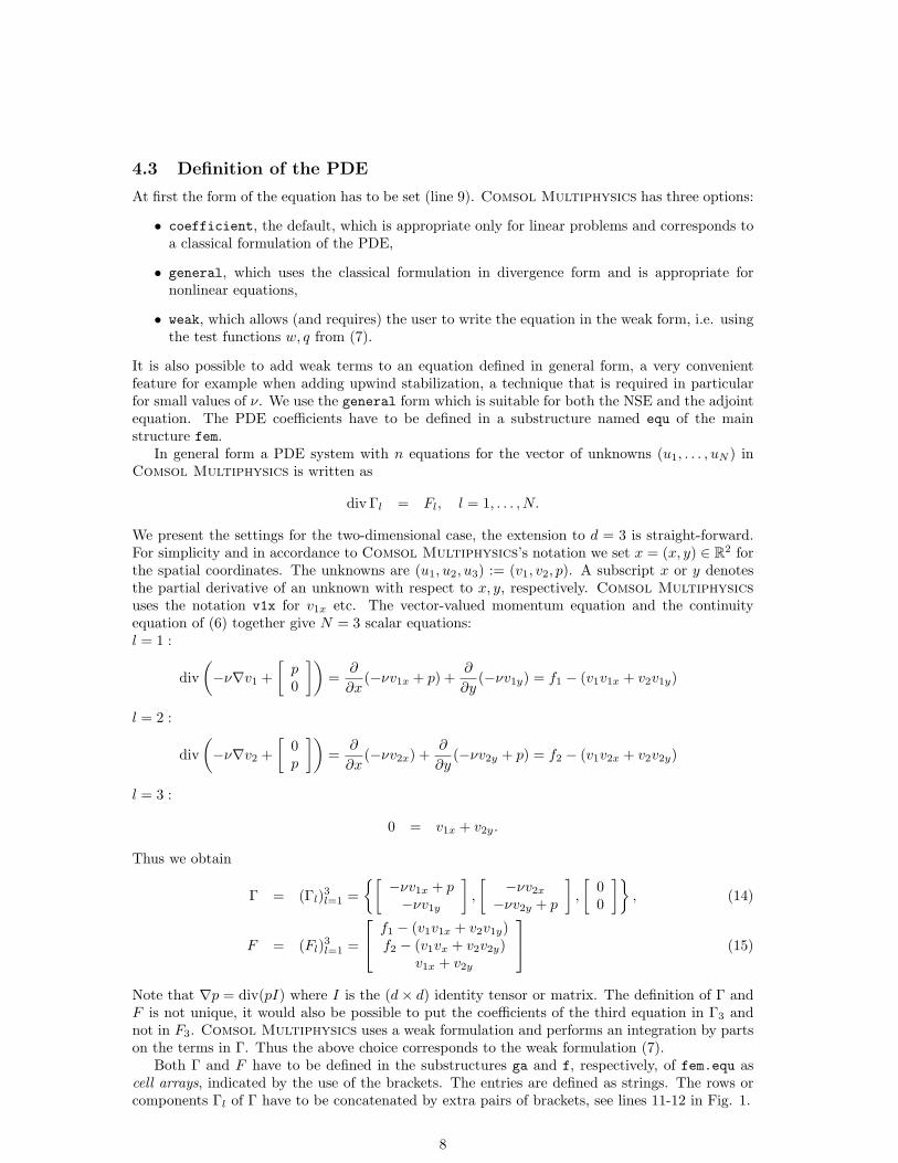
In general form a PDE system with n equations for the vector of unknowns (u1, . . . , uN ) inComsol Multiphysics is written as

div Γl = Fl, l = 1, . . . , N.

We present the settings for the two-dimensional case, the extension to d = 3 is straight-forward.For simplicity and in accordance to Comsol Multiphysics’s notation we set x = (x, y) ∈ R2 forthe spatial coordinates. The unknowns are (u1, u2, u3) := (v1, v2, p). A subscript x or y denotesthe partial derivative of an unknown with respect to x, y, respectively. Comsol Multiphysicsuses the notation v1x for v1x etc. The vector-valued momentum equation and the continuityequation of (6) together give N = 3 scalar equations:l = 1 :

div(−ν∇v1 +

[p0

])=

∂

∂x(−νv1x + p) +

∂

∂y(−νv1y) = f1 − (v1v1x + v2v1y)

l = 2 :

div(−ν∇v2 +

[0p

])=

∂

∂x(−νv2x) +

∂

∂y(−νv2y + p) = f2 − (v1v2x + v2v2y)

l = 3 :

0 = v1x + v2y.

Thus we obtain

Γ = (Γl)3l=1 =[

−νv1x + p−νv1y

],

[−νv2x

−νv2y + p

],

[00

], (14)

F = (Fl)3l=1 =

f1 − (v1v1x + v2v1y)f2 − (v1vx + v2v2y)

v1x + v2y

(15)

Note that ∇p = div(pI) where I is the (d× d) identity tensor or matrix. The definition of Γ andF is not unique, it would also be possible to put the coefficients of the third equation in Γ3 andnot in F3. Comsol Multiphysics uses a weak formulation and performs an integration by partson the terms in Γ. Thus the above choice corresponds to the weak formulation (7).

Both Γ and F have to be defined in the substructures ga and f, respectively, of fem.equ ascell arrays, indicated by the use of the brackets. The entries are defined as strings. The rows orcomponents Γl of Γ have to be concatenated by extra pairs of brackets, see lines 11-12 in Fig. 1.

8

Note also that for both Γ and F there are two outer pairs of brackets. Comsol Multiphysicsallows the user to define different regions in the computational domain with different PDE settingsin each region (so-called multi-physics). For each of these regions different coefficients Γ and Fmay be defined, and they are concatenated in by the outmost pairs of brackets. Although we donot use this feature here, still this additional pair of brackets is required.

The constant ν that is used in Γ has to be defined as element of the substructure fem.constbefore (see line 9).

In line 10 we defined, again as cell array of strings, the right-hand side vector f = (f1, f2) tobe zero. For this purpose the expressions F1, F2 have been defined in the substructure expr ofthe structure fem.equ, and they have been given the value ’0’ as string. It is also possible toinsert the inhomogeneities directly in the array F , without using the substructure expr. Usingthe spatial coordinates x, y and any of Matlab’s built-in functions arbitrary inhomogeneities canbe defined. The definition of user-defined functions will be described later on.

4.4 Boundary conditions

The substructure fem.bnd defines the boundary conditions. Based on the initial geometry differentboundary sections can be defined (line 13): The cavity initially has four edges, on one of them(edge 3, the upper one) we impose inhomogeneous Dirichlet conditions, on the other three we havehomogeneous Dirichlet conditions. The numbering of the edges has to be found by trial and error,since it has no obvious order. The indices of the boundary parts of the edges have to be put inthe array fem.bnd.ind.

The boundary conditions on each boundary section are written as

−η · Γl = Gl +M∑

m=1

∂Rm

∂ulµm, l = 1, . . . , N

Rm = 0, m = 1, . . . ,M

on ∂Ω. (16)

The µm are artificially introduced Lagrange multipliers, i.e. additional free variables. Depend-ing on the choice of the vectors R = (Rm)M

m=1 and G = (Gl)Nl=1 (implemented in fem.bnd.r

and fem.bnd.g, both zero by default) Dirichlet, natural and mixed boundary conditions can berealized.

To define Dirichlet conditions G = 0 is set. Then the first equation in (16) imposes no conditionon the unknowns because of the free Lagrange multipliers. By defining R the Dirichlet conditionsare specified. For the example of the driven cavity we have

v1 = g1, v2 = 0 i.e. R1 = v1 − g1, R2 = v2 on Σd1

v1 = 0, v2 = 0 i.e. R1 = v1, R2 = v2 on Σd2

for some given function g1. This function (here set to the constant 1.0) and the vector R areimplemented in lines 14-15, where fem.bnd.r is a cell array with two components, one for everyboundary section defined in fem.bnd.ind.

For a boundary section with free outflow (or ”do nothing”) condition R = 0 is set. TheLagrange multipliers are meaningless, and since

−η · Γ1 = −η ·(−ν∇v1 +

[p0

])= ν∂ηv1 − pη1 = G1,

−η · Γ2 = −η ·(−ν∇v2 +

[0p

])= ν∂ηv2 − pη2 = G2,

−η · Γ3 = 0 = G3

(17)

in the NSE case the first equation in (16) gives the desired natural (here free outflow) condition ifG = 0 is set. An example is given in Fig. 2.

9

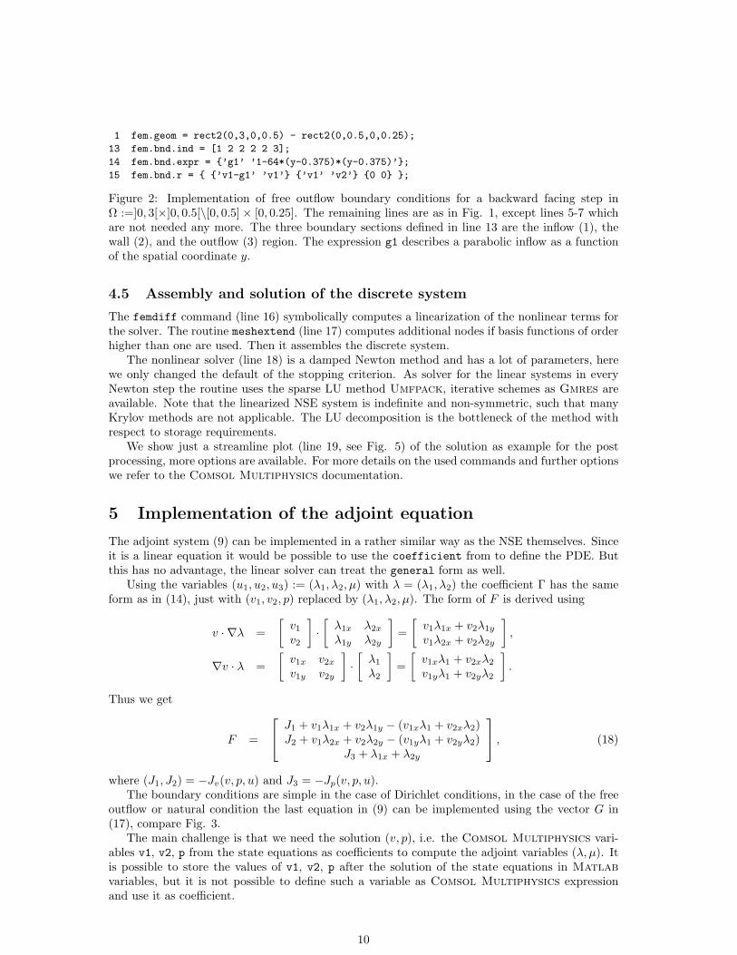
1 fem.geom = rect2(0,3,0,0.5) - rect2(0,0.5,0,0.25);

13 fem.bnd.ind = [1 2 2 2 2 3];

14 fem.bnd.expr = ’g1’ ’1-64*(y-0.375)*(y-0.375)’;

15 fem.bnd.r = ’v1-g1’ ’v1’ ’v1’ ’v2’ 0 0 ;

Figure 2: Implementation of free outflow boundary conditions for a backward facing step inΩ :=]0, 3[×]0, 0.5[\[0, 0.5] × [0, 0.25]. The remaining lines are as in Fig. 1, except lines 5-7 whichare not needed any more. The three boundary sections defined in line 13 are the inflow (1), thewall (2), and the outflow (3) region. The expression g1 describes a parabolic inflow as a functionof the spatial coordinate y.

4.5 Assembly and solution of the discrete system

The femdiff command (line 16) symbolically computes a linearization of the nonlinear terms forthe solver. The routine meshextend (line 17) computes additional nodes if basis functions of orderhigher than one are used. Then it assembles the discrete system.

The nonlinear solver (line 18) is a damped Newton method and has a lot of parameters, herewe only changed the default of the stopping criterion. As solver for the linear systems in everyNewton step the routine uses the sparse LU method Umfpack, iterative schemes as Gmres areavailable. Note that the linearized NSE system is indefinite and non-symmetric, such that manyKrylov methods are not applicable. The LU decomposition is the bottleneck of the method withrespect to storage requirements.

We show just a streamline plot (line 19, see Fig. 5) of the solution as example for the postprocessing, more options are available. For more details on the used commands and further optionswe refer to the Comsol Multiphysics documentation.

5 Implementation of the adjoint equation

The adjoint system (9) can be implemented in a rather similar way as the NSE themselves. Sinceit is a linear equation it would be possible to use the coefficient from to define the PDE. Butthis has no advantage, the linear solver can treat the general form as well.

Using the variables (u1, u2, u3) := (λ1, λ2, µ) with λ = (λ1, λ2) the coefficient Γ has the sameform as in (14), just with (v1, v2, p) replaced by (λ1, λ2, µ). The form of F is derived using

v · ∇λ =[

v1

v2

]·[

λ1x λ2x

λ1y λ2y

]=

[v1λ1x + v2λ1y

v1λ2x + v2λ2y

],

∇v · λ =[

v1x v2x

v1y v2y

]·[

λ1

λ2

]=

[v1xλ1 + v2xλ2

v1yλ1 + v2yλ2

].

Thus we get

F =

J1 + v1λ1x + v2λ1y − (v1xλ1 + v2xλ2)J2 + v1λ2x + v2λ2y − (v1yλ1 + v2yλ2)

J3 + λ1x + λ2y

, (18)

where (J1, J2) = −Jv(v, p, u) and J3 = −Jp(v, p, u).The boundary conditions are simple in the case of Dirichlet conditions, in the case of the free

outflow or natural condition the last equation in (9) can be implemented using the vector G in(17), compare Fig. 3.

The main challenge is that we need the solution (v, p), i.e. the Comsol Multiphysics vari-ables v1, v2, p from the state equations as coefficients to compute the adjoint variables (λ, µ). Itis possible to store the values of v1, v2, p after the solution of the state equations in Matlabvariables, but it is not possible to define such a variable as Comsol Multiphysics expressionand use it as coefficient.

10

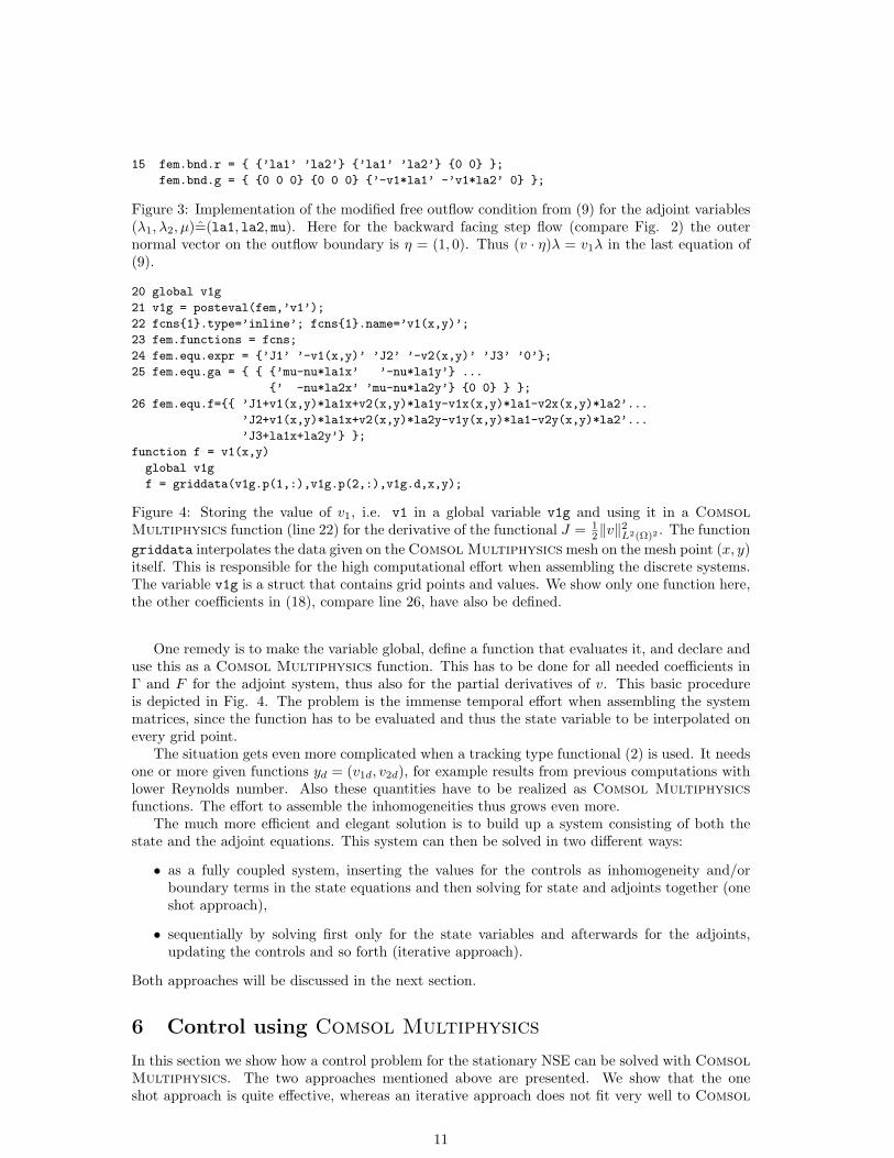
15 fem.bnd.r = ’la1’ ’la2’ ’la1’ ’la2’ 0 0 ;

fem.bnd.g = 0 0 0 0 0 0 ’-v1*la1’ -’v1*la2’ 0 ;

Figure 3: Implementation of the modified free outflow condition from (9) for the adjoint variables(λ1, λ2, µ)=(la1, la2, mu). Here for the backward facing step flow (compare Fig. 2) the outernormal vector on the outflow boundary is η = (1, 0). Thus (v · η)λ = v1λ in the last equation of(9).

20 global v1g

21 v1g = posteval(fem,’v1’);

22 fcns1.type=’inline’; fcns1.name=’v1(x,y)’;

23 fem.functions = fcns;

24 fem.equ.expr = ’J1’ ’-v1(x,y)’ ’J2’ ’-v2(x,y)’ ’J3’ ’0’;

25 fem.equ.ga = ’mu-nu*la1x’ ’-nu*la1y’ ...

’ -nu*la2x’ ’mu-nu*la2y’ 0 0 ;

26 fem.equ.f= ’J1+v1(x,y)*la1x+v2(x,y)*la1y-v1x(x,y)*la1-v2x(x,y)*la2’...

’J2+v1(x,y)*la1x+v2(x,y)*la2y-v1y(x,y)*la1-v2y(x,y)*la2’...

’J3+la1x+la2y’ ;

function f = v1(x,y)

global v1g

f = griddata(v1g.p(1,:),v1g.p(2,:),v1g.d,x,y);

Figure 4: Storing the value of v1, i.e. v1 in a global variable v1g and using it in a ComsolMultiphysics function (line 22) for the derivative of the functional J = 1

2‖v‖2L2(Ω)2 . The function

griddata interpolates the data given on the Comsol Multiphysics mesh on the mesh point (x, y)itself. This is responsible for the high computational effort when assembling the discrete systems.The variable v1g is a struct that contains grid points and values. We show only one function here,the other coefficients in (18), compare line 26, have also be defined.

One remedy is to make the variable global, define a function that evaluates it, and declare anduse this as a Comsol Multiphysics function. This has to be done for all needed coefficients inΓ and F for the adjoint system, thus also for the partial derivatives of v. This basic procedureis depicted in Fig. 4. The problem is the immense temporal effort when assembling the systemmatrices, since the function has to be evaluated and thus the state variable to be interpolated onevery grid point.

The situation gets even more complicated when a tracking type functional (2) is used. It needsone or more given functions yd = (v1d, v2d), for example results from previous computations withlower Reynolds number. Also these quantities have to be realized as Comsol Multiphysicsfunctions. The effort to assemble the inhomogeneities thus grows even more.

The much more efficient and elegant solution is to build up a system consisting of both thestate and the adjoint equations. This system can then be solved in two different ways:

• as a fully coupled system, inserting the values for the controls as inhomogeneity and/orboundary terms in the state equations and then solving for state and adjoints together (oneshot approach),

• sequentially by solving first only for the state variables and afterwards for the adjoints,updating the controls and so forth (iterative approach).

Both approaches will be discussed in the next section.

6 Control using Comsol Multiphysics

In this section we show how a control problem for the stationary NSE can be solved with ComsolMultiphysics. The two approaches mentioned above are presented. We show that the oneshot approach is quite effective, whereas an iterative approach does not fit very well to Comsol

11

Figure 5: Uncontrolled driven cavity flow for ν = 1 (desired state, left), uncontrolled (middle) andcontrolled for ν = 1

1000 . The cost (without regularization term) was reduced to 0.5 % comparedto the uncontrolled flow. 1625 pressure nodes.

Multiphysics’s built-in PDE representation and data structures. Examples for distributed andboundary control implementations are given.

6.1 One shot approach

The optimality system (4) summarizes the necessary conditions for a solution of the constrainedproblem (3). Thus one may try to solve it directly. Then the second equation which gives therelation between adjoint variable and control is inserted for the control in the state equation, anda coupled system of state and adjoint equation is solved.

Following the idea to solve the whole optimality system and using the coupling informationbetween adjoints and control from (10) leads to rather short implementations that we present inthe following subsections.

If the state equation is non-linear an appropriate solver is Newton’s method (note that theadjoint equation is always linear). The resulting optimization algorithm is a variant of the Sqpmethod, see for example [9]. In every step of the newton iteration a linear system has to be solved.The one shot approach doubles the size of the whole system, and thus also of the linearized systemsto be solved in each Newton step. For an iterative solver storing issues may become crucial here.

6.1.1 Distributed control for driven cavity flow.

The first example that we consider is a typical test case for the NSE. The computational domain isthe unit square, where on the upper and sometimes also on the lower part of the boundary a velocityfield is prescribed. The two lateral boundaries are considered as wall, thus there homogeneousDirichlet boundary conditions are imposed. There is no outflow boundary, i.e. Σn = ∅. If aconstant positive horizontal velocity is imposed on the top and v is set to zero at the bottom, theflow shows one big eddy turning clockwise. Depending on the Reynolds number the center of thisvortex moves to the right and its shape slightly changes.

The Comsol Multiphysics script is shown in Fig. 6 for distributed control, compare alsoFig. 1. Setting ν = 1

1000 we tried to achieve the flow for ν = 1 by imposing distributed control onthe whole domain. Since we use a tracking type functional we add a third set of equations for thedesired state and solve for it firstly. The results are shown in Fig. 5 and 9.

In this example the one shot approach with Comsol Multiphysics’s damped Newton al-gorithm worked very well, it converged in six steps for a regularization parameter of 0.01, andproduced a satisfying result, even without choosing a special initial value for the nonlinear itera-tion.

6.1.2 Boundary control for backward facing step channel flow.

In this second example we try to minimize the region of back-flow in a channel with a backwardfacing step. Free outflow conditions were imposed at the end of the channel. For low values of ν

12

3 fem.dim = ’v1d’ ’v2d’ ’pd’ ’v1’ ’v2’ ’p’ ’la1’ ’la2’ ’mu’;

4 fem.shape = [2 2 1 2 2 1 2 2 1];

5 fem.pnt.constr = 0 0 ’-pd’ 0 0 ’-p’ 0 0 ’-mu’ 0;

10 fem.equ.expr = ’J1’ ’v1d-u’ ’J2’ ’v2d-v’;

11 fem.equ.ga = ’pd-nu*v1dx’ ’-nu*v1dy’ ...

’-nu*v2dx’ ’pd-nu*v2dy’ 0 0 ...

’p-nu*v1x’ ’-nu*v1y’ ...

’-nu*v2x’ ’p-nu*v2y’ 0 0 ...

’mu-nu*la1x’ ’-nu*la1y’ ...

’-nu*la2x’ ’mu-nu*la2y’ 0 0 ;

12 fem.equ.f = ’-v1d*v1dx-v2d*v1dy’ ...

’-v1d*v2dx-v2d*v2dy’ ’v1dx+v2dy’ ...

’la1/alpha-v1*v1x-v2*v1y’ ...

’la2/alpha-v1*v2x-v2*v2y’ ’v1x+v2y’ ...

’J1+v1*la1x+v2*la1y-v1x*la1-v2x*la2’ ...

’J2+v1*la2x+v2*la2y-v1y*la1-v2y*la2’ ’la1x+la2y’;

15 fem.bnd.r = ’v1d-g1’ ’v2d’ ’v1-g1’ ’v2’ ’la1’ ’la2’ ...

’v1d’ ’v2d’ ’v1’ ’v2’ ’la1’ ’la2’ ;

18 fem.sol = femnlin(fem,’solcomp’,’v1d’ ’v2d’ ’pd’);

19 fem.const = ’nu’ ’0.001’ ’alpha’ ’0.01’;

21 fem.xmesh = meshextend(fem);

22 fem.sol = femnlin(fem, ...

’solcomp’,’v1’ ’v2’ ’p’ ’la1’ ’la2’ ’mu’,’u’,fem.sol);

23 J = postint(fem,’(v1-v1d)*(v1-v1d)+(v2-v2d)*(v2-v2d)’)/2 ...

+ postint(fem,’(la1*la1+la2*la2)/alpha’)/2;

Figure 6: Script for distributed control of a driven cavity flow in 2-D. Lines 1-2, 6-9, 13-14, and16-17 as in Fig. 1. The desired state is computed in line 18. The optimality system is set up andsolved in lines 19-22. Note the repetition of the meshextend command. In line 22 the last twoadditional parameters passed to the solver ensure that the solution component u from the fem.solsubstructure is used in the current computation. The output of a solver is stored in the variablefem.sol.u, no matter what names were given to the unknowns in line 3. Here fem.sol.u containsthe output v1d, v2d, pd from the computation in line 19. Line 23 evaluates the cost functional.

13

Figure 7: Uncontrolled (top) and controlled (middle: α = 1, bottom: α = 0.1) backward facingstep flow, ν = 1

1000 . The cost was reduced to 37% and 5.9%, respectively. 3427 pressure nodes,computations with a finer grid (13469 nodes) were also possible on a machine with 1 GByte RAM,and produced similar results.

there is a long separation bubble behind the step. Aim was to reduce this bubble, compare Fig 7.For this purpose we used the cost functional (compare [4])

J(v, uB) =12

∥∥∥∥[minv1, 0

min−v2, 0

]∥∥∥∥2

L2(Ω)2+

α

2‖uB‖2

L2(Σc)2. (19)

The velocity on the vertical boundary Σc := 0.5×]0, 0.25[ was used as control parameter. Thecrucial point is to get access to the normal derivative of the adjoint variable (see (12)) that becomesthe boundary condition in the state equations of the optimality system. From (12) and (17) weget

uB = −(ν∂ηλ− µη)/α =1α

[−ν(λ1xη1 + λ1yη2) + µη1

−ν(λ2xη1 + λ2yη2) + µη2

].

Conveniently Comsol Multiphysics allows to access the components η1, η2 of the outer normalvector via the variables nx and ny such that uB can be implemented as boundary condition.The Comsol Multiphysics script is shown in Fig. 8. Here no desired state was used, so thecorresponding variables and equations are skipped. Fig. 7 shows that the optimization was quitesuccessful for α = 1 and 0.1, the computed control is shown in Fig. 9. The convergence was slowerthan for the driven cavity example, the damped Newton method took 41 iterations from the start(with zero as initial value) for α = 1 and additional 17 ones in a restart with α = 0.1. It is alsopossible to increase the stopping criterion for the first iteration (e.g. ’ntol’,1e-2 for α = 1), andrestart from there. Note that ν = 1

1000 is quite low for control in this configuration.

6.2 Sequential or iterative approach

As contrast to the one shot approach it is possible to solve the state equation firstly, then theadjoint equation with the just computed state, and perform an update of the control using theLagrange multiplier and formula (5). This procedure is then iterated until convergence is reached.To avoid the implementation of the optimization algorithm one may use a library, or in the

14

3 fem.dim = ’v1’ ’v2’ ’p’ ’la1’ ’la2’ ’mu’;

4 fem.shape = [2 2 1 2 2 1];

10 fem.equ.expr = ’J1’ ’-min(v1,0)’ ’J2’ ’min(-v2,0)’;

11 fem.equ.ga = ’p-nu*v1x’ ’-nu*v1y’ ...

’-nu*v2x’ ’p-nu*v2y’ 0 0 ...

’mu-nu*la1x’ ’-nu*la1y’ ...

’-nu*la2x’ ’mu-nu*la2y’ 0 0 ;

12 fem.equ.f = ’-v1*v1x-v2*v1y’ ’-v1*v2x-v2*v2y’ ’v1x+v2y’ ...

’J1+v1*la1x+v2*la1y-v1x*la1-v2x*la2’ ...

’J2+v1*la2x+v2*la2y-v1y*la1-v2y*la2’ ’la1x+la2y’;

15 fem.bnd.r = ’v1-g1’ ’v2’ ’la1’ ’la2’ ’v1’ ’v2’ ’la1’ ’la2’ 0 0 0 0 ...

’v1+(nu*(la1x*nx+la1y*ny)-mu*nx)/alpha’ ...

’v2+(nu*(la2x*nx+la2y*ny)-mu*ny)/alpha’ ’la1’ ’la2’ ;

17 fem.bnd.g = 0 0 0 0 0 0 0 0 0 0 0 0 ...

0 0 0 ’-v1*la1’ ’-v1*la2’ 0 0 0 0 0 0 0 ;

19 fem.const.nu = 0.001;

20 fem.const.alpha = 1;

21 fem.xmesh = meshextend(fem);

22 fem.sol = femnlin(fem,’maxiter’,50,’ntol’,1e-4);

23 fem.const.alpha = 0.1;

24 fem.xmesh = meshextend(fem);

25 fem.sol = femnlin(fem,’init’,fem.sol,’minstep’,1e-8,’ntol’,1e-4);

26 J = postint(fem,’min(u,0)*min(u,0)+min(-v,0)*min(-v,0)’)/2 ...

+ postint(fem,’((nu*(la1x*nx+la1y*ny)-mu*nx)*(nu*(la1x*nx+la1y*ny)-mu*nx) ...

+(nu*(la2x*nx+la2y*ny)-mu*ny)*(nu*(la2x*nx+la2y*ny)-mu*ny))/alpha’,...

’edim’,1,’dl’,4)/2;

Figure 8: Script for boundary control of a backward facing step. Lines 1, 13-14 are as in Fig. 2,lines 2, 8, 16 as in Fig. 1. Lines 23-25 show a restart with smaller regularization parameter. Theoption init indicates that the previous solution in fem.sol is taken as initial guess, minstep isthe minimal damping factor for Newton’s method, maxiter the maximum number of steps. Line26 shows the evaluation of the cost.

Figure 9: Control for driven cavity (left, α = 0.01) and backward facing step (α = 0.1), ν = 11000 .

15

1 global uglob nodes n

2 fcns1.type=’inline’; fcns1.name=’u1(x,y)’;

3 fcns2.type=’inline’; fcns2.name=’u2(x,y)’;

4 fem.functions = fcns;

5 fem.sol = femnlin(fem,’solcomp’,’v1’ ’v2’ ’p’);

6 u = posteval(fem,’v1’); nodes = u.p; n = length(u.d);

7 options = optimset(’GradObj’,’on’);

8 u = fminunc(@cost,u,options,fem);

9 function [f,df] = cost(u,fem)

10 global uglob

11 uglob = u;

12 fem.xmesh = meshextend(fem);

13 fem.sol = femnlin(fem,’solcomp’,’v1’ ’v2’ ’p’);

14 f=postint(fem,’min(v1,0)*min(v1,0)+min(-v2,0)*min(-v2,0)’)/2...

+postint(fem,’(u1(x,y)*u1(x,y)+u2(x,y)*u2(x,y))/alpha’)72;

15 fem.sol = femlin(fem,’solcomp’,’la1’ ’la2’ ’mu’,’u’,fem.sol);

16 la1 = posteval(fem,’la1’); la2 = posteval(fem,’la2’);

17 df = fem.const.alpha*u-[la1.d,la2.d];

18 function f = u1(x,y)

19 global uglob nodes n

20 f = griddata(nodes(1,:),nodes(2,:),uglob(1:n),x,y);

Figure 10: Part of a script for an iterative solution for distributed control. The global copy ugloband the storing of the coordinates and number of grid points (line 6) is needed for the functionsu1, u2 that realize the control.

Matlab case, a toolbox routine. Then J and J ′(u) have to be implemented, where the formerincorporates the solution of the state, the latter in addition the solution of the adjoint equation.The advantage is that the systems to be solved have ”only” the size of the state equation, whereasin the one-shot approach the coupled system of double size has to be solved. Moreover differentoptimization routines may be used, and additional constraints may also be incorporated withoutchanging the underlying Comsol Multiphysics setting. We assume that we use an optimizationroutine that needs the implementation of the cost in a function that takes the current control (sayu) as parameter, and returns the value of the cost and the gradient (say J and DJ) as output.This is for example the case for optimization routines in Matlab’s optimization toolbox. Anunconstrained minimization using a quasi-Newton method is performed in the script which ispartially shown in Fig. 10. Line 7 specifies that the user-defined function cost also returns thegradient. The last parameter fem for the optimization routine in line 8 is passed to the functioncost as second parameter. The update formulas (11) or (13) for the control (implemented in line17 in Fig. 10), it is inevitable to realize the control as a Comsol Multiphysics function (seelines 2-4,14,18-20). The efficiency problems that result from this fact have already been discussedin Section 5. For the adjoint equation they could be avoided. This is the main reason that theone shot approach is superior when working with Comsol Multiphysics.

6.3 A 3-D example

At the end we briefly show how the 2-D examples can be extended to three space dimensions.The basic proceeding should be clear, and the implementation of the equations for the additionalvariables v3, la3 is straight forward. An geometry initialization is shown in Fig. 11.

A crucial point in 3-D computations is the necessary storage. We thus just show an examplewith a rather coarse mesh (864 pressure nodes) and ν = 0.01, α = 1 in Fig. 12. Here boundarycontrol an the vertical wall of the step was used to reduce the cost from (19), with v2 replaced byv3.

16

fem.geom = block3(3,1,1,’base’,’corner’,’pos’,[0 -0.5 -0.5]) ...

- block3(0.5,1,0.5,’base’,’corner’,’pos’,[0 -0.5 -0.5]);

fem.bnd.expr = ’g1’ ’(1-4*y*y)*(1-16*(z-0.25)*(z-0.25))’;

fem.bnd.ind = [1 2 2 2 2 4 3];

Figure 11: Geometry initialization for a backward facing step in 3-D.

Figure 12: Uncontrolled (left) and controlled backward facing step flow in 3-D for ν = 1500 . The

results are similar to the 2-D case for high Reynolds number, compare Fig. 7. Only a coarse gridwith 470 pressure nodes was used. The cost was reduced to 6.4%.

7 Summary and Outlook

The Comsol Multiphysics programming environment is offers the flexibility to solve state andadjoint equations, and thus whole optimality systems for stationary PDE-constrained controlproblems. The implementation of the adjoint equation can be done with reasonable effort andknowledge of the internal Comsol Multiphysics data structure. The effort for this, comparedto a complete implementation in another language or environment (as Matlab), is quite small.The built-in damped Newton solver is rather effective also to solve optimality systems. Due tothe internal representation of equations in Comsol Multiphysics it turned out to be moreappropriate for the control problems than using other optimization routines and coupling themwith Comsol Multiphysics. The successful application to stationary NSE encourages us toassume that also other nonlinear equations could be considered. Three dimensional problems canbe handled, the bottleneck is the needed storage for the direct sparse linear solvers. In 3-D aswitch to iterative solvers that are also provided in Comsol Multiphysics has to be considered.In principle time-dependent applications are also possible, but they are beyond the scope of thispaper.

References

[1] F. Abergel and E. Casas. Some optimal control problems associated to the stationary Navier-Stokes equation. In J.-I. Diaz et al., editor, Mathematics, climate, and environment, Res.Notes Appl. Math., volume 27, pages 213–220. Masson, Paris, 1993.

[2] Comsol Inc. http://www.femlab.com.

[3] J.C. de los Reyes and K. Kunisch. A semi-smooth Newton method for control constrainedboundary optimal control of the Navier-Stokes equations. Nonlinear Analysis, 62:1289–1316,2005.

[4] M. Desai and K. Ito. Optimal controls of Navier-Stokes equations. SIAM J. Control Optim.,32(5):1428–1446, 1994.

[5] V. Girault and P.-A. Raviart. Finite Element Methods for Navier-Stokes Equations. SpringerSeries in Computational Mathematics 5, New York, 1986.

[6] M.D. Gunzburger, L. Hou, and T.P. Svobodny. Analysis and finite element approximationof optimal control problems for the stationary Navier-Stokes equations with distributed andneumann controls. Math. Comput., 57(195):123–151, 1991.

17

[7] J.L. Lions. Optimal Control of Systems Governed by Partial Differential Equations. Springer,New York, 1971.

[8] The Mathworks, Inc. http://www.matlab.com.

[9] J. Nocedal and S.J. Wright. Numerical Optimization. Springer, New York, 2000.

[10] T. Roubicek and F. Troltzsch. Lipschitz stability of optimal controls for the steady stateNavier-Stokes equations. Control and Cybernetics, 32:683–705, 2003.

[11] T. Slawig. A formula for the derivative with respect to domain variations in Navier-Stokesflow based on an embedding domain method. SIAM J. Contr. Optim., 42(2):495–512, 2003.

[12] R. Temam. Navier-Stokes Equations. North-Holland, Amsterdam, 1979.

18