techniques for high-performance distributed …
TRANSCRIPT

TECHNIQUES FOR
HIGH-PERFORMANCE
DISTRIBUTED COMPUTING IN
COMPUTATIONAL FLUID MECHANICS
by
Lisandro Daniel Dalcın
Dissertation submitted to the Postgraduate Department of the
FACULTAD DE INGENIERIA Y CIENCIAS HIDRICAS
of the
UNIVERSIDAD NACIONAL DEL LITORAL
in partial fulfillment of the requirements for the degree of
Doctor en Ingenierıa - Mencion Mecanica Computacional
2008


A mis padres Elda y Daniel,
a mi hermana Marianela,
a mi novia Julieta,
a la memoria de mi tia Araceli
y de mi abuela Lucrecia.

Author Legal Declaration
This dissertation have been submitted to the Postgraduate Department of
the Facultad de Ingenierıa y Ciencias Hıdricas in partial fulfillment of the
requirements the degree of Doctor in Engineering - Field of Computational
Mechanics of the Universidad Nacional del Litoral. A copy of this document
will be available at the University Library and it will be subjected to the
Library’s legal normative.
Some parts of the work presented in this thesis have been (or are going
to be) published in the following journals: Computer Methods in Applied Me-
chanics and Engineering, Journal of Parallel and Distributed Computing and
Advances in Engineering Software.
Lisandro Daniel Dalcın
c© Copyright by
Lisandro Daniel Dalcın
2008


Contents
Preface ix
1 Scientific Computing with Python 1
1.1 The Python Programming Language . . . . . . . . . . . . . . . 1
1.2 Tools for Scientific Computing . . . . . . . . . . . . . . . . . . . 2
1.2.1 Numerical Python . . . . . . . . . . . . . . . . . . . . . 2
1.2.2 Scientific Tools for Python . . . . . . . . . . . . . . . . . 2
1.2.3 Fortran to Python Interface Generator . . . . . . . . . . 2
1.2.4 Simplified Wrapper and Interface Generator . . . . . . . 3
2 MPI for Python 5
2.1 An Overview of MPI . . . . . . . . . . . . . . . . . . . . . . . . 6
2.1.1 History . . . . . . . . . . . . . . . . . . . . . . . . . . . . 7
2.1.2 Main Features of MPI . . . . . . . . . . . . . . . . . . . 8
2.2 Related work on MPI and Python . . . . . . . . . . . . . . . . . 11
2.3 Design and Implementation . . . . . . . . . . . . . . . . . . . . 12
2.3.1 Accessing MPI Functionalities . . . . . . . . . . . . . . . 13
2.3.2 Communicating Python Objects . . . . . . . . . . . . . . 14
2.4 Using MPI for Python . . . . . . . . . . . . . . . . . . . . . . . 16
2.4.1 Classical Message-Passing Communication . . . . . . . . 16
2.4.2 Dynamic Process Management . . . . . . . . . . . . . . . 22
2.4.3 One-sided Operations . . . . . . . . . . . . . . . . . . . . 23
2.4.4 Parallel Input/Output Operations . . . . . . . . . . . . . 26
2.5 Efficiency Tests . . . . . . . . . . . . . . . . . . . . . . . . . . . 28
2.5.1 Measuring Overhead in Message Passing Operations . . . 29
v

vi CONTENTS
2.5.2 Comparing Wall-Clock Timings for Collective Commu-
nication Operations . . . . . . . . . . . . . . . . . . . . . 35
3 PETSc for Python 39
3.1 An Overview of PETSc . . . . . . . . . . . . . . . . . . . . . . . 40
3.1.1 Main Features of PETSc . . . . . . . . . . . . . . . . . . 40
3.2 Design and Implementation . . . . . . . . . . . . . . . . . . . . 45
3.3 Using PETSc for Python . . . . . . . . . . . . . . . . . . . . . . 46
3.3.1 Working with Vectors . . . . . . . . . . . . . . . . . . . . 46
3.3.2 Working with Matrices . . . . . . . . . . . . . . . . . . . 46
3.3.3 Using Linear Solvers . . . . . . . . . . . . . . . . . . . . 48
3.3.4 Using Nonlinear Solvers . . . . . . . . . . . . . . . . . . 49
3.4 Efficiency Tests . . . . . . . . . . . . . . . . . . . . . . . . . . . 52
3.4.1 The Poisson Problem . . . . . . . . . . . . . . . . . . . . 52
3.4.2 A Matrix-Free Approach for the Linear Problem . . . . . 53
3.4.3 Some Selected Krylov-Based Iterative Methods . . . . . 55
3.4.4 Measuring Overhead . . . . . . . . . . . . . . . . . . . . 58
4 Electrokinetic Flow in Microfluidic Chips 65
4.1 Background . . . . . . . . . . . . . . . . . . . . . . . . . . . . . 66
4.2 Theoretical Modeling . . . . . . . . . . . . . . . . . . . . . . . . 68
4.2.1 Governing Equations . . . . . . . . . . . . . . . . . . . . 68
4.2.2 Electrokinetic Phenomena . . . . . . . . . . . . . . . . . 69
4.3 Numerical Simulations . . . . . . . . . . . . . . . . . . . . . . . 73
4.4 Classical Domain Decomposition Methods . . . . . . . . . . . . 78
4.4.1 A Model Problem . . . . . . . . . . . . . . . . . . . . . . 79
4.4.2 Additive Schwarz Preconditioning . . . . . . . . . . . . . 81
5 Final Remarks 91
5.1 Impact of this work . . . . . . . . . . . . . . . . . . . . . . . . . 91
5.2 Publications . . . . . . . . . . . . . . . . . . . . . . . . . . . . . 93

List of Figures
2.1 Access to MPI COMM RANK from Python. . . . . . . . . . . . . . . 14
2.2 Sending and Receiving general Python objects. . . . . . . . . . . 17
2.3 Nonblocking Communication of Array Data. . . . . . . . . . . . 20
2.4 Broadcasting general Python objects. . . . . . . . . . . . . . . . 21
2.5 Distributed Dense Matrix-Vector Product. . . . . . . . . . . . . 21
2.6 Computing π with a Master/Worker Model in Python. . . . . . 23
2.7 Computing π with a Master/Worker Model in C++. . . . . . . 24
2.8 Permutation of Block-Distributed 1D Arrays (slow version). . . 26
2.9 Permutation of Block-Distributed 1D Arrays (fast version). . . . 27
2.10 Input/Output of Block-Distributed 2D Arrays. . . . . . . . . . . 28
2.11 Python code for timing a blocking Send and Receive. . . . . . . 31
2.12 Python code for timing a bidirectional Send/Receive. . . . . . . 31
2.13 Python code for timing All-To-All. . . . . . . . . . . . . . . . . 31
2.14 Throughput and overhead in blocking Send and Receive. . . . . 32
2.15 Throughput and overhead in bidirectional Send/Receive. . . . . 33
2.16 Throughput and overhead in All-To-All. . . . . . . . . . . . . . 34
2.17 Timing in Broadcast. . . . . . . . . . . . . . . . . . . . . . . . . 35
2.18 Timing in Scatter. . . . . . . . . . . . . . . . . . . . . . . . . . 36
2.19 Timing in Gather. . . . . . . . . . . . . . . . . . . . . . . . . . . 36
2.20 Timing in Gather to All. . . . . . . . . . . . . . . . . . . . . . . 37
2.21 Timing in All to All Scatter/Gather. . . . . . . . . . . . . . . . 37
3.1 Basic Implementation of Conjugate Gradient Method. . . . . . . 47
3.2 Assembling a Sparse Matrix in Parallel. . . . . . . . . . . . . . . 48
3.3 Solving a Linear Problem in Parallel. . . . . . . . . . . . . . . . 49
vii

viii LIST OF FIGURES
3.4 Nonlinear Residual Function for the Bratu Problem. . . . . . . . 51
3.5 Solving a Nonlinear Problem with Matrix-Free Jacobians. . . . . 51
3.6 Defining a Matrix-Free Operator for the Poisson Problem. . . . 54
3.7 Solving a Matrix-Free Linear Problem with PETSc for Python. . 54
3.8 Defining a Matrix-Free Operator, C implementation. . . . . . . 56
3.9 Solving a Matrix-Free Linear Problem, C implementation. . . . 57
3.10 Comparing Overhead Results for CG and GMRES (30). . . . . . 59
3.11 PETSc for Python Overhead using CG . . . . . . . . . . . . . . . 60
3.12 Residual History using CG . . . . . . . . . . . . . . . . . . . . . 60
3.13 PETSc for Python Overhead using MINRES . . . . . . . . . . . 61
3.14 Residual History using MINRES . . . . . . . . . . . . . . . . . . 61
3.15 PETSc for Python Overhead using BiCGStab. . . . . . . . . . . 62
3.16 Residual History using BiCGStab. . . . . . . . . . . . . . . . . . 62
3.17 PETSc for Python Overhead using GMRES (30). . . . . . . . . . 63
3.18 Residual History using GMRES (30). . . . . . . . . . . . . . . . 63
4.1 Microfluidic Chips. . . . . . . . . . . . . . . . . . . . . . . . . . 66
4.2 The Diffuse Double Layer and the Debye Length. . . . . . . . . 71
4.3 Electroosmotic Flow. . . . . . . . . . . . . . . . . . . . . . . . . 72
4.4 Geometry of the Microchannel Network. . . . . . . . . . . . . . 74
4.5 Initial Na+ and Ka+ Ions Concentrations (mol/3m) . . . . . . . 75
4.6 Injection Stage. . . . . . . . . . . . . . . . . . . . . . . . . . . . 76
4.7 Separation Stage. . . . . . . . . . . . . . . . . . . . . . . . . . . 77
4.8 Model Problem. . . . . . . . . . . . . . . . . . . . . . . . . . . . 80
4.9 Additive Schwarz Preconditioning (Mesh #1). . . . . . . . . . . 85
4.10 Additive Schwarz Preconditioning (Mesh #2). . . . . . . . . . . 86
4.11 Additive Schwarz Preconditioning (Mesh #3). . . . . . . . . . . 87
4.12 Additive Schwarz Preconditioning (Mesh #3). . . . . . . . . . . 88
4.13 Additive Schwarz Preconditioning (32 processors). . . . . . . . . 89

Preface
Parallel Computing and Message Passing
Among many parallel computational models, message-passing has proven to
be an effective one. This paradigm is specially suited for (but not limited
to) distributed memory architectures. Although there are many variations,
the basic concept of processes communicating through messages has been well
understood from long time.
Portable message-passing parallel programming used to be a nightmare
in the past. Developers of parallel applications were faced to many pro-
prietary, incompatible and architecture-dependent message-passing libraries.
Code portability was hampered by the differences between them. Fortunately,
this situation definitely changed after the Message Passing Interface (MPI)
standard specification appeared and rapidly gained acceptance.
Since its release, the MPI specification has become the leading standard for
message-passing libraries in the world of parallel computers. Nowadays, MPI
is being widely used in the most demanding scientific and engineering appli-
cations related to modeling, simulation, design, and signal processing. Over
the last years, high performance computing has finally become an affordable
resource to everyone with needs of increased computing power. The conjunc-
tion of commodity hardware and high quality open source operating systems
and software packages strongly influenced the now widespread popularity of
Beowulf [1] class clusters and cluster of workstations.
An important subset of scientific and engineering applications deals with
problems modeled by partial differential equations on two-dimensional and
ix

x PREFACE
tree-dimensional domains. In those kind of applications, numerical methods
are the only practical way to attack complex problems. Those methods nec-
essarily involve a discretization of the governing equations at the continuum
level. From this discretization process, systems of linear and nonlinear equa-
tions arise. When those systems of equations are very large, parallel processing
is mandatory in order to solve them in reasonable time frames.
The popularity and availability of parallel computing resources on dis-
tributed memory architectures, together with the high degree of portability
offered by the MPI specification, strongly motivated the development of gen-
eral purpose, multi-platform software components tailored to efficiently solve
large-scale linear and nonlinear problems.
Currently, PETSc [2] y Trilinos [3] are the most complete and advanced
general purpose libraries available for supporting large-scale simulations in sci-
ence and engineering. PETSc[2, 4], the Portable Extensible Toolkit for Scien-
tific Computation, is a suite of state of the art algorithms and data structures
for the solution of problems arising on scientific and engineering applications.
It is being developed at Argonne National Laboratory, USA. PETSc is specially
suited for those modeled by partial differential equations, of large-scale nature,
and targeted for parallel, distributed-memory computing environments [5].
High-Level Languages for Scientific Computing
In parallel to the aforementioned trends, the popularity of some general high-
level, general purpose scientific computing environments–such as MATLAB
and IDL in the commercial side or Octave and Scilab in the open source side–
has increased considerably. Users simply feel much more productive in such
interactive environments providing tight integration of simulation and visual-
ization. They are alleviated of low-level details associated to compilation and
linking steps, memory management and input/output of the more traditional
scientific programming languages like Fortran, C, and even C++.
Recently, the Python programming language [6, 7] has attracted the at-
tention of many end-users and developers in the scientific community. Python
offers a clean and simple syntax, is a very powerful language, and allows skilled

xi
users to build their own computing environment, tailored to their specific needs
and based on their favorite high-performance Fortran, C, or C++ codes. So-
phisticated but easy to use and well integrated packages are available for in-
teractive command-line work, efficient multi-dimensional array processing, 2D
and 3D visualization, and other scientific computing tasks.
About This Thesis
Although a lot of progress has been made in theory as well as practice, the true
costs of accessing parallel environments are still largely dominated by software.
The number of end-user parallelized applications is still very small, as well as
the number of people affected to their development. Engineers and scientists
not specialized in programming or numerical computing, and even small and
medium size software companies, hardly ever considered developing their own
parallelized code. High performance computing is traditionally associated with
software development using compiled languages. However, in typical applica-
tions programs, only a small part of the code is time-critical enough to require
the efficiency of compiled languages. The rest of the code is generally related
to memory management, error handling, input/output, and user interaction,
and those are usually the most error-prone and time-consuming lines of code
to write and debug in the whole development process. Interpreted high-level
languages can be really advantageous for these kind of tasks.
This thesis reports the attempts to facilitate the access to high-performance
parallel computing resources within a Python programming environment. The
target audience are all members of the scientific and engineering community
using Python on a regular basis as the supporting environment for develop-
ing applications and performing numerical simulations. The target computing
platforms range from multiple-processor and/or multiple-core desktop comput-
ers, clusters of workstations or dedicated computing nodes either with stan-
dard or special network interconnects, to high-performance shared memory
machines. The net result of this effort are two open source and public domain
packages, MPI for Python (known in short as mpi4py) and PETSc for Python
(known in short as petsc4py).

xii PREFACE
MPI for Python [8, 9, 10], is an open-source, public-domain software project
that provides bindings of the Message Passing Interface (MPI) standard for
the Python programming language. MPI for Python is a general-purpose and
full-featured package targeting the development of parallel application codes in
Python. Its facilities allow parallel Python programs to easily exploit multiple
processors. MPI for Python employs a back-end MPI implementation, thus
being immediately available on any parallel environment providing access to
any MPI library.
PETSc for Python [11] is an open-source, public-domain software project
that provides access to the Portable, Extensible Toolkit for Scientific
Computation (PETSc) libraries within the Python programming language.
PETSc for Python is a general-purpose and full-featured package. Its facilities
allow sequential and parallel Python applications to exploit state of the art
algorithms and data structures readily available in PETSc.
MPI for Python and PETSc for Python packages are fully integrated to
PETSc-FEM [12], an MPI and PETSc based parallel, multiphysics, finite el-
ements code. Within a parallel Python programming environment, this soft-
ware infrastructure supported research activities related to the simulation of
electrophoretic processes in microfluidic chips. This work is part of a mul-
tidisciplinary effort oriented to design and develop these devices in order to
improve current techniques in clinical analysis and early diagnosis of cancer.
Chapter 1
Scientific Computing with
Python
This chapter is an introductory one. Section 1.1 provides a general overview
of the Python programing language. Section 1.2 comments some fundamental
packages and development tools commonly used in the scientific community
taking advantage of both the high-level features of Python and the execution
performance of traditional compiled languages like C, C ++ and Fortran.
1.1 The Python Programming Language
Python [6] is a modern, easy to learn, powerful programming language. It
has efficient high-level data structures and a simple but effective approach to
object-oriented programming.
Python’s elegant syntax, together with its interpreted nature, make it an
ideal language for scripting and rapid application development. It supports
modules and packages, which encourages program modularity and code reuse.
Additionally, It is easily extended with new functions and data types imple-
mented in C, C++, and Fortran. The Python interpreter and the extensive
standard library are freely available in source or binary form for all major
platforms, and can be freely distributed.
1
2 CHAPTER 1. SCIENTIFIC COMPUTING WITH PYTHON
1.2 Tools for Scientific Computing
1.2.1 Numerical Python
NumPy [13] is an open source project providing the fundamental library needed
for serious scientific computing with Python.
NumPy provides a powerful multi-dimensional array object with advanced
and efficient array slicing operations to select array elements and convenient
array reshaping methods. Additionally, NumPy contains three sub-libraries
with numerical routines providing basic linear algebra operations, basic Fourier
transforms and sophisticated capabilities for random number generation.
1.2.2 Scientific Tools for Python
SciPy [14] is an open source library of scientific tools for Python. It depends on
the NumPy library, and it gathers a variety of high level science and engineering
modules together as a single package.
SciPy provides modules for statistics, optimization, numerical integration,
linear algebra, Fourier transforms, signal and image processing, genetic algo-
rithms, special functions, and many more.
1.2.3 Fortran to Python Interface Generator
F2PY [15], the Fortran to Python Interface Generator, provides a connection
between the Python and Fortran programming languages.
F2PY is a development tool for creating Python extension modules from
special signature files or directly from annotated Fortran source files. The
signature files, or the Fortran source files with additonal annotations included
as comments, contain all the information (function names, arguments and their
types, etc.) that is needed to construct convenient Python bindings to Fortran
functions. The F2PY -generated Python extension modules enable Python
codes to call those Fortran 77/90/95 routines. In addition, F2PY provides
the required support for transparently accessing Fortran 77 common blocks or
Fortran 90/95 module data.

1.2. TOOLS FOR SCIENTIFIC COMPUTING 3
Fortran (and specially Fortran 90 and above) is a convenient compiled
language for efficiently implementing lengthy computations involving multi-
dimensional arrays. Although NumPy provides similar and higher-level ca-
pabilities, there are situations where selected, numerically intensive parts of
Python applications still requiere the efficiency of a compiled language for pro-
cessing huge amounts of data in deeply-nested loops. Additionally, state of the
art implementations of many commonly used algorithms are readily available
and implemented in Fortran. In a Python programming environment, F2PY
is then the tool of choice for taking advantage of the speed-up of compiled
Fortran code and integrating existing Fortran libraries.
1.2.4 Simplified Wrapper and Interface Generator
SWIG [16], the Simplified Wrapper and Interface Generator, is an interface
compiler that connects programs written in C and C++ with a variety of
scripting languages.
SWIG works by taking the declarations found in C/C++ header files and
using them to generate the wrapper code that scripting languages need to
access the underlying C/C++ code. In addition, SWIG provides a variety of
customization features that let developers to tailor the wrapping process to
suit specific application needs.
Originally developed in 1995, SWIG was first used by scientists (in the
Theoretical Physics Division at Los Alamos National Laboratory, USA) for
building user interfaces to molecular dynamic simulation codes running on
the Connection Machine 5 supercomputer. In this environment, scientists
needed to work with huge amounts of simulation data, complex hardware,
and a constantly changing code base. The use of a Python scripting language
interface provided a simple yet highly flexible foundation for solving these
types of problems [17]. This software infrastructure nowadays supports the
largest-scale molecular dynamic simulations in the world [18].
Although SWIG was originally developed for scientific applications, it has
since evolved into a general purpose tool that is used in a wide variety of
applications–in fact almost anything where C/C++ programming is involved.


Chapter 2
MPI for Python
This chapter is devoted to describing MPI for Python, an open-source, public-
domain software project that provides bindings of the Message Passing Inter-
face (MPI) standard for the Python programming language.
MPI for Python is a general-purpose and full-featured package targeting
the development of parallel application codes in Python. It provides core
facilities that allow parallel Python programs to exploit multiple processors.
Sequential Python applications can also take advantages of MPI for Python
by communicating through the MPI layer with external, independent parallel
modules, possibly written in other languages like C++,C, or Fortran.
MPI for Python employs a back-end MPI implementation, thus being im-
mediately available on any parallel environment providing access to any MPI
library. Those environments range from multiple-processor and/or multiple-
core desktop computers, clusters of workstations or dedicated computing nodes
with standard or special network interconnects, to high-performance shared
memory machines.
Section 2.1 presents a general description about MPI and the main concepts
contained in the MPI-1 and MPI-2 specifications. Section 2.2 reviews some
previous works related to MPI and Python; these works provided invaluable
guidance for designing and implementing MPI for Python.
Section 2.3 describes the general design and implementation of MPI for
Python through a mixed language, C-Python approach. Additionally, two
5

6 CHAPTER 2. MPI FOR PYTHON
mechanisms for inter-process data communication at the Python-level are dis-
cussed. Section 2.4 presents a general overview of the many MPI concepts
and functionalities accessible through MPI for Python. Additionally, a series
of short, self-contained example codes with their corresponding discussions is
provided. These examples show how to use MPI for Python for implementing
parallel Python codes with the help of MPI.
Finally, section 2.5 presents some efficiency tests and discusses their results.
Those test are focused on measuring and comparing wall clock timings of
selected communication operations implemented both in C and Python.
2.1 An Overview of MPI
Among many parallel computational models, message-passing has proven to
be an effective one. This paradigm is specially suited for (but not limited
to) distributed memory architectures and is used in today’s most demanding
scientific and engineering application related to modeling, simulation, design,
and signal processing.
MPI, the Message Passing Interface, is a standardized, portable message-
passing system designed to function on a wide variety of parallel computers.
The standard defines the syntax and semantics of library routines (MPI is not a
programming language extension) and allows users to write portable programs
in the main scientific programming languages (Fortran, C, and C++).
MPI defines a high-level abstraction for fast and portable inter-process
communication [19, 20]. Applications can run in clusters of (possibly hetero-
geneous) workstations or dedicated nodes, (symmetric) multiprocessors ma-
chines, or even a mixture of both. MPI hides all the low-level details, like net-
working or shared memory management, simplifying development and main-
taining portability, without sacrificing performance.

2.1. AN OVERVIEW OF MPI 7
2.1.1 History
Portable message-passing parallel programming used to be a nightmare in
the past because of the many incompatible options developers were faced
to. Proprietary message passing libraries were available on several parallel
computer systems, and were used to develop significant parallel applications.
However, the code portability of those applications was hampered by the
huge differences between these communication libraries. At the same time,
several public-domain libraries were available. They had demonstrated that
portable message-passing systems could be implemented without sacrificing
performance.
In 1992, the Message Interface Passing (MPI) Forum [21] was born,
teaming-up a group of researchers from academia and industry involving over
80 people from 40 organizations. This group undertook the effort of defining
the syntax and semantics of a standard core of library routines that would be
useful for a wide range of users and efficiently implementable on a wide range
of parallel computing systems and environments.
The fist MPI standard specification [22], also known as MPI-1, appeared
in 1994 and immediately gained widespread acceptance. After two years, a
second version of the standard [23] was released. Although being completely
backwards compatible, MPI-2 introduced some clarifications for features al-
ready available in MPI-1 but also many extensions and new functionalities.
The MPI specifications is nowadays the leading standard for message-
passing libraries in the world of parallel computers. Implementations are avail-
able from vendors of high-performance computers and well known open source
projects like MPICH [24, 25] and Open MPI [26, 27].
The MPI Forum has been dormant for nearly a decade. However, in late
2006 it reactivated for the purpose of clarifying current MPI issues, renew
membership and interest, explore future opportunities, and possibly defining
a new standard level. At the time of this witting, clarifications to MPI-2
are being actively discussed and new working groups are being established for
generating a future MPI-3 specification.

8 CHAPTER 2. MPI FOR PYTHON
2.1.2 Main Features of MPI
Communication Domains and Process Groups
MPI communication operations occurs within a specific communication do-
main through an abstraction called communicator. Communicators are built
from groups of participating processes and provide a communication context
for the members of those groups.
Process groups enable parallel applications to assign processing resources
in sets of cooperating processes in order to perform independent work. Com-
municators provide a safe isolation mechanism for implementing independent
parallel library routines and mixing them with user code; message passing oper-
ations within different communication domains are guaranteed to not conflict.
Processes within a group can communicate each other (including itself)
through an intracommunicator ; they can also communicate with processes
within another group through an intercommunicator.
Intracommunicators are intended for communication between processes
that are members of the same group. They have one fixed attribute: its process
group. Additionally, they can have an optional, predefined attribute: a virtual
topology (either Cartesian or a general graph) describing the logical layout of
the processes in the group. This extra, optional topology attribute is useful
in many ways: it can help the underlying MPI runtime system to map pro-
cesses onto hardware; it simplifies the implementation of common algorithmic
concepts.
Intercommunicators are intended to be used for performing communica-
tion operations between processes that are members of two disjoint groups.
They provide a natural way of enabling communication between independent
modules in complex, multidisciplinary applications.
Point-to-Point Communication
Point to point communication is a fundamental capability of massage passing
systems. This mechanism enables the transmittal of data between a pair of
processes, one side sending, the other, receiving.

2.1. AN OVERVIEW OF MPI 9
MPI provides a set of send and receive functions allowing the communi-
cation of typed data with an associated tag. The type information enables
the conversion of data representation from one architecture to another in the
case of heterogeneous computing environments; additionally, it allows the rep-
resentation of non-contiguous data layouts and user-defined datatypes, thus
avoiding the overhead of (otherwise unavoidable) packing/unpacking opera-
tions. The tag information allows selectivity of messages at the receiving end.
MPI provides basic send and receive functions that are blocking. These
functions block the caller until the data buffers involved in the communication
can be safely reused by the application program.
MPI also provides nonblocking send and receive functions. They allow the
possible overlap of communication and computation. Non-blocking communi-
cation always come in two parts: posting functions, which begin the requested
operation; and test-for-completion functions, which allow to discover whether
the requested operation has completed.
Collective Communication
Collective communications allow the transmittal of data between multiple pro-
cesses of a group simultaneously. The syntax and semantics of collective func-
tions is consistent with point-to-point communication. Collective functions
communicate typed data, but messages are not paired with an associated tag ;
selectivity of messages is implied in the calling order. Additionally, collective
functions come in blocking versions only.
The more commonly used collective communication operations are the fol-
lowing.
• Barrier synchronization across all group members.
• Global communication functions
– Broadcast data from one member to all members of a group.
– Gather data from all members to one member of a group.
– Scatter data from one member to all members of a group.
10 CHAPTER 2. MPI FOR PYTHON
• Global reduction operations such as sum, maximum, minimum, etc.
Dynamic Process Management
In the context of the MPI-1 specification, a parallel application is static; that is,
no processes can be added to or deleted from a running application after it has
been started. Fortunately, this limitation was addressed in MPI-2. The new
specification added a process management model providing a basic interface
between an application and external resources and process managers.
This MPI-2 extension can be really useful, especially for sequential ap-
plications built on top of parallel modules, or parallel applications with a
client/server model. The MPI-2 process model provides a mechanism to cre-
ate new processes and establish communication between them and the existing
MPI application. It also provides mechanisms to establish communication be-
tween two existing MPI applications, even when one did not “start” the other.
One-Sided Operations
One-sided communications (also called Remote Memory Access, RMA) sup-
plements the traditional two-sided, send/receive based MPI communication
model with a one-sided, put/get based interface. One-sided communication
that can take advantage of the capabilities of highly specialized network hard-
ware. Additionally, this extension lowers latency and software overhead in
applications written using a shared-memory-like paradigm.
The MPI specification revolves around the use of objects called windows ;
they intuitively specify regions of a process’s memory that have been made
available for remote read and write operations. The published memory blocks
can be accessed through three functions for put (remote send), get (remote
write), and accumulate (remote update or reduction) data items. A much
larger number of functions support different synchronization styles; the se-
mantics of these synchronization operations are fairly complex.
2.2. RELATED WORK ON MPI AND PYTHON 11
Parallel Input/Output
The POSIX [28] standard provides a model of a widely portable file system.
However, the optimization needed for parallel input/output cannot be achieved
with this generic interface. In order to ensure efficiency and scalability, the
underlying parallel input/output system must provide a high-level interface
supporting partitioning of file data among processes and a collective interface
supporting complete transfers of global data structures between process mem-
ories and files. Additionally, further efficiencies can be gained via support for
asynchronous input/output, strided accesses to data, and control over phys-
ical file layout on storage devices. This scenario motivated the inclusion in
the MPI-2 standard of a custom interface in order to support more elaborated
parallel input/output operations.
The MPI specification for parallel input/output revolves around the use
objects called files. As defined by MPI, files are not just contiguous byte
streams. Instead, they are regarded as ordered collections of typed data items.
MPI supports sequential or random access to any integral set of these items.
Furthermore, files are opened collectively by a group of processes.
The common patterns for accessing a shared file (broadcast, scatter, gather,
reduction) is expressed by using user-defined datatypes. Compared to the com-
munication patterns of point-to-point and collective communications, this ap-
proach has the advantage of added flexibility and expressiveness. Data access
operations (read and write) are defined for different kinds of positioning (using
explicit offsets, individual file pointers, and shared file pointers), coordination
(non-collective and collective), and synchronism (blocking, nonblocking, and
split collective with begin/end phases).
2.2 Related work on MPI and Python
As MPI for Python started and evolved, many ideas were borrowed from other
well known open source projects related to MPI and Python.
OOMPI [29, 30] is an excellent C++ class library specification layered on
top of the C bindings encapsulating MPI into a functional class hierarchy. This
12 CHAPTER 2. MPI FOR PYTHON
library provides a flexible and intuitive interface by adding some abstractions,
like Ports and Messages, which enrich and simplify the syntax.
pyMPI [31] rebuilds the Python interpreter and adds a built-in module
for message passing. It permits interactive parallel runs, which are useful
for learning and debugging, and provides an environment suitable for basic
parallel programing. There is limited support for defining new communicators
and process topologies; support for intercommunicators is absent. General
Python objects can be messaged between processors; there is some support for
direct communication of numeric arrays.
Pypar [32] is a rather minimal Python interface to MPI. There is no support
for constructing new communicators or defining process topologies. It does not
require the Python interpreter to be modified or recompiled. General Python
objects of any type can be communicated. There is also good support for
communicating numeric arrays and practically full MPI bandwidth can be
achieved.
Scientific Python [33] provides a collection of Python modules that are
useful for scientific computing. Among them, there is an interface to MPI. This
interface is incomplete and does not resemble the MPI specification. However,
there is good support for efficiently communicating numeric arrays.
2.3 Design and Implementation
Python has enough networking capabilities as to develop an implementation of
MPI in “pure Python”, i.e., without using compiled languages or depending on
the availability of a third-party MPI library. The main advantage of such kind
of implementation is surely portability (at least as much as Python provides);
there is no need to rely on any foreign language or library. However, such an
approach would have many severe limitations as to the point being considered
a nonsense. Vendor-provided MPI implementations take advantage of special
features of target platforms otherwise unavailable. Additionally, there are
many useful and high-quality MPI-based parallel libraries; almost all them are
written in compiled languages. The development of an MPI package based in
calls to any available MPI implementation will sensibly ease the integration of

2.3. DESIGN AND IMPLEMENTATION 13
other parallel tools in Python. Finally, Python is really easy to extend and
connect with external software components developed in compiled languages;
it is expected that “wrapping” any existing MPI library would require by
far less development effort than reimplementing from scratch the full MPI
specification.
In subsection 2.2 some previous attempts of integrating MPI and Python
were mentioned. However, all of them lack from completeness and interface
conformance with the standard specification. MPI for Python provides an
interface designed with focus on translating MPI syntax and semantics from
the standard MPI-2 C++ bindings to Python. As syntax translation from
C++ to Python is generally straightforward, any user with some knowledge
of those C++ bindings should be able to use this package without need of
learning a new interface specification. Of course, accessing MPI functionalities
from Python necessarily requires some adjustments and enhancements in order
to follow common language idioms and take better advantage of such a high-
level environment.
2.3.1 Accessing MPI Functionalities
MPI for Python provides access to almost all MPI features through a two-layer,
mixed language approach.
In the low-level layer, a set of extension modules written in C provide access
to all functions and predefined constants in the MPI specification. Addition-
ally, this C code implements some basic machinery for converting any MPI
object between its Python representation (i.e. an instance of a specific Python
class) and C representation (i.e. an opaque MPI handle). All this conversion
machinery is carefully designed for interoperability; any MPI object created
and managed through MPI for Python can be easily recovered at the C level
and the reused for any purpose (e.g. it can be used for calling a routine in any
MPI-based library accessible through a C, C++, or Fortran interface).
In the high-level layer, a module written in Python defines all class hi-
erarchies, class methods and functions. This Python code is supported by
the low-level C extension modules commented above. The final user interface
14 CHAPTER 2. MPI FOR PYTHON
closely resembles the standard MPI-2 bindings for C++.
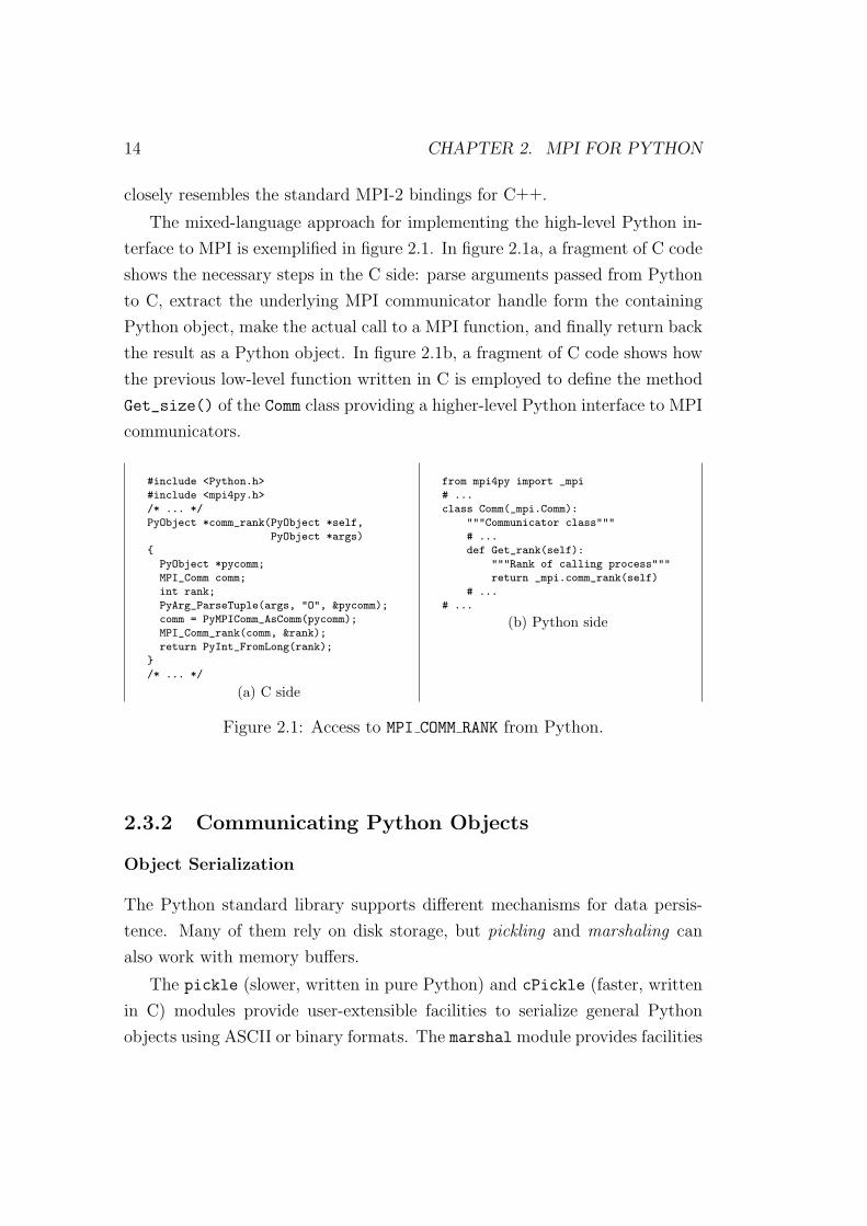
The mixed-language approach for implementing the high-level Python in-
terface to MPI is exemplified in figure 2.1. In figure 2.1a, a fragment of C code
shows the necessary steps in the C side: parse arguments passed from Python
to C, extract the underlying MPI communicator handle form the containing
Python object, make the actual call to a MPI function, and finally return back
the result as a Python object. In figure 2.1b, a fragment of C code shows how
the previous low-level function written in C is employed to define the method
Get_size() of the Comm class providing a higher-level Python interface to MPI
communicators.
#include <Python.h>
#include <mpi4py.h>
/* ... */
PyObject *comm_rank(PyObject *self,
PyObject *args)
PyObject *pycomm;
MPI_Comm comm;
int rank;
PyArg_ParseTuple(args, "O", &pycomm);
comm = PyMPIComm_AsComm(pycomm);
MPI_Comm_rank(comm, &rank);
return PyInt_FromLong(rank);
/* ... */
(a) C side
from mpi4py import _mpi
# ...
class Comm(_mpi.Comm):
"""Communicator class"""
# ...
def Get_rank(self):
"""Rank of calling process"""
return _mpi.comm_rank(self)
# ...
# ...
(b) Python side
Figure 2.1: Access to MPI COMM RANK from Python.
2.3.2 Communicating Python Objects
Object Serialization
The Python standard library supports different mechanisms for data persis-
tence. Many of them rely on disk storage, but pickling and marshaling can
also work with memory buffers.
The pickle (slower, written in pure Python) and cPickle (faster, written
in C) modules provide user-extensible facilities to serialize general Python
objects using ASCII or binary formats. The marshal module provides facilities
2.3. DESIGN AND IMPLEMENTATION 15
to serialize built-in Python objects using a binary format specific to Python,
but independent of machine architecture issues.
MPI for Python can communicate any general or built-in Python object
taking advantage of the features provided by cPickle and marshal modules.
Their functionalities are wrapped in two classes, Pickle and Marshal, defining
dump() and load() methods. These are simple extensions, being completely
unobtrusive for user-defined classes to participate (they actually use the stan-
dard pickle protocol), but carefully optimized for serialization of Python ob-
jects on memory streams.
This approach is also fully extensible; that is, users are allowed to define
new, custom serializers implementing the generic dump()/load() interface.
Any provided or user-defined serializer can be attached to communicator in-
stances. They will be routinely used to build binary representations of objects
to communicate (at sending processes), and restoring them back (at receiving
processes).
Memory Buffers
Although simple and general, the serialization approach (i.e. pickling and
unpickling) previously discussed imposes important overheads in memory as
well as processor usage, especially in the scenario of objects with large mem-
ory footprints being communicated. The reasons for this are simple. Pickling
general Python objects, ranging from primitive or container built-in types to
user-defined classes, necessarily requires computer resources. Processing is
needed for dispatching the appropriate serialization method (that depends on
the type of the object) and doing the actual packing. Additional memory is
always needed, and if its total amount in not known a priori, many realloca-
tions can occur. Indeed, in the case of large numeric arrays, this is certainly
unacceptable and precludes communication of objects occupying half or more
of the available memory resources.
MPI for Python supports direct communication of any object exporting the
single-segment buffer interface. This interface is a standard Python mechanism
provided by some types (e.g. strings and numeric arrays), allowing access in the

16 CHAPTER 2. MPI FOR PYTHON
C side to a contiguous memory buffer (i.e. address and length) containing the
relevant data. This feature, in conjunction with the capability of constructing
user-defined MPI datatypes describing complicated memory layouts, enables
the implementation of many algorithms involving multidimensional numeric
arrays (e.g. image processing, fast Fourier transforms, finite difference schemes
on structured Cartesian grids) directly in Python, with negligible overhead,
and almost as fast as compiled Fortran, C, or C++ codes.
2.4 Using MPI for Python
This section presents a general overview and some examples of many MPI
concepts and functionalities readily available in MPI for Python. Discussed
features range from classical MPI-1 message-passing communication operations
to and more advances MPI-2 operations like dynamic process management,
one-sided communication, and parallel input/output.
2.4.1 Classical Message-Passing Communication
Communicators
In MPI for Python, Comm is the base class of communicators. Communica-
tor size and calling process rank can be respectively obtained with methods
Get_size() and Get_rank().
The Intracomm and Intercomm classes are derived from the Comm class.
The Is_inter() method (and Is_intra(), provided for convenience, it is not
part of the MPI specification) is defined for communicator objects and can be
used to determine the particular communicator class.
The two predefined intracommunicator instances are available: COMM_WORLD
and COMM_SELF (or WORLD and SELF, they are just aliases provided for conve-
nience). From them, new communicators can be created as needed.
New communicator instances can be obtained with the Clone() method of
Comm objects, the Dup() and Split() methods of Intracomm and Intercomm
objects, and methods Create_intercomm() and Merge() of Intracomm and
Intercomm objects respectively.
2.4. USING MPI FOR PYTHON 17
Virtual topologies (Cartcomm and Graphcomm classes, both being a special-
ization of Intracomm class) are fully supported. New instances can be obtained
from intracommunicator instances with factory methods Create_cart() and
Create_graph() of Intracomm class.
The associated process group can be retrieved from a communicator by
calling the Get_group() method, which returns am instance of the Group
class. Set operations with Group objects like like Union(), Intersect() and
Difference() are fully supported, as well as the creation of new communica-
tors from these groups.
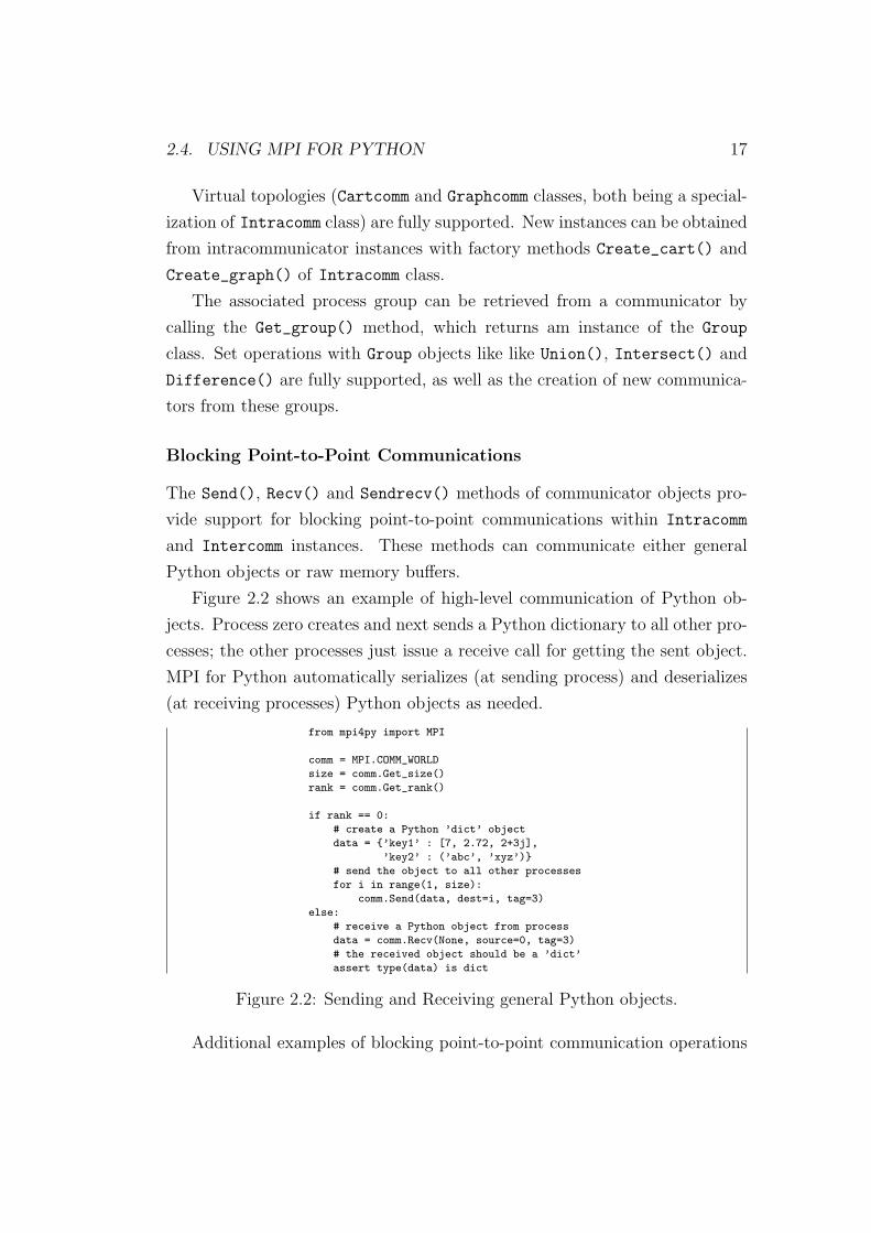
Blocking Point-to-Point Communications
The Send(), Recv() and Sendrecv() methods of communicator objects pro-
vide support for blocking point-to-point communications within Intracomm
and Intercomm instances. These methods can communicate either general
Python objects or raw memory buffers.
Figure 2.2 shows an example of high-level communication of Python ob-
jects. Process zero creates and next sends a Python dictionary to all other pro-
cesses; the other processes just issue a receive call for getting the sent object.
MPI for Python automatically serializes (at sending process) and deserializes
(at receiving processes) Python objects as needed.
from mpi4py import MPI
comm = MPI.COMM_WORLD
size = comm.Get_size()
rank = comm.Get_rank()
if rank == 0:
# create a Python ’dict’ object
data = ’key1’ : [7, 2.72, 2+3j],
’key2’ : (’abc’, ’xyz’)
# send the object to all other processes
for i in range(1, size):
comm.Send(data, dest=i, tag=3)
else:
# receive a Python object from process
data = comm.Recv(None, source=0, tag=3)
# the received object should be a ’dict’
assert type(data) is dict
Figure 2.2: Sending and Receiving general Python objects.
Additional examples of blocking point-to-point communication operations

18 CHAPTER 2. MPI FOR PYTHON
can be found in section 2.5. Those examples show how MPI for Python can
efficiently communicate NumPy arrays by directly using their exposed memory
buffers, thus avoiding the overhead of serialization and deserialization steps.
Nonblocking Point-to-Point Communications
On many systems, performance can be significantly increased by overlapping
communication and computation. This is particularly true on systems where
communication can be executed autonomously by an intelligent, dedicated
communication controller. Nonblocking communication is a mechanism pro-
vided by MPI in order to support such overlap.
The inherently asynchronous nature of nonblocking communications cur-
rently imposes some restrictions in what can be communicated through MPI
for Python. Communication of memory buffers, as described in section 2.3.2
is fully supported. However, communication of general Python objects using
serialization, as described in section 2.3.2, is possible but not transparent since
objects must be explicitly serialized at sending processes, while receiving pro-
cesses must first provide a memory buffer large enough to hold the incoming
message and next recover the original object.
The Isend() and Irecv() methods of the Comm class initiate a send and
receive operation respectively. These methods return a Request instance,
uniquely identifying the started operation. Its completion can be managed
using the Test(), Wait(), and Cancel() methods of the Request class. The
management of Request objects and associated memory buffers involved in
communication requires a careful, rather low-level coordination. Users must
ensure that objects exposing their memory buffers are not accessed at the
Python level while they are involved in nonblocking message-passing opera-
tions.
Often a communication with the same argument list is repeatedly exe-
cuted within an inner loop. In such cases, communication can be further
optimized by using persistent communication, a particular case of nonblocking
communication allowing the reduction of the overhead between processes and
communication controllers. Furthermore , this kind of optimization can also

2.4. USING MPI FOR PYTHON 19
alleviate the extra call overheads associated to interpreted, dynamic languages
like Python. The Send_init() and Recv_init() methods of the Comm class
create a persistent request for a send and receive operation respectively. These
methods return an instance of the Prequest class, a subclass of the Request
class. The actual communication can be effectively started using the Start()
method, and its completion can be managed as previously described.
Figure 2.3 shows a mixture of blocking and nonblocking point-to-point
communication involving three processes. Process zero and two send data to
process three using standard, blocking send calls; the messages have the same
length but they are tagged with different values. Process three issues two
nonblocking receive calls specifying a wildcard value for the source process, but
explicitly selecting messages by their tag values; the data is received in a two-
dimensional array with two rows and enough columns to hold each message.
The nonblocking receive calls at process three return request objects, they
are next waited for completion. While messages are in transit (between the
post-receive calls and the call waiting for completion ), process three can use
its computing resources for any other local task, thus effectively overlapping
computation with communication. The outcome of this message interchange
is the following: process three receives the message sent from process zero in
the second row of the local data array; the the message sent from process one
is received in the fist row of the local data array.
Collective Communications
The Bcast(), Scatter(), Gather(), Allgather() and Alltoall() meth-
ods of Intracomm instances provide support for collective communications.
Those methods can communicate either general Python objects or raw memory
buffers. The vector variants (which can communicate different amounts of data
at each process) Scatterv(), Gatherv(), Allgatherv() and Alltoallv()
are also supported, they can only communicate objects exposing raw memory
buffers.
Global reduction operations are accessible through the Reduce(),
Allreduce(), Scan() and Exscan() methods. All the predefined (i.e., SUM,

20 CHAPTER 2. MPI FOR PYTHON
from mpi4py import MPI
import numpy
comm = MPI.COMM_WORLD
size = comm.Get_size()
rank = comm.Get_rank()
assert size == 3, ’run me in three processes’
if rank == 0:
# send a thousand integers to process two
data = numpy.ones(1000, dtype=’i’)
comm.Send([data, MPI.INT], dest=2, tag=35)
elif rank == 1:
# send a thousand integers to process two
data = numpy.arange(1000, dtype=’i’)
comm.Send([data, MPI.INT], dest=2, tag=46)
else:
# create empty integer 2d array with two rows and
# a thousand columns to hold received data
data = numpy.empty([2, 1000], dtype=’i’)
# post for receive 1000 integers with message tag 46
# from any source and store it in the firt row
req1 = comm.Irecv([data[0, :], MPI.INT],
source=MPI.ANY_SOURCE, tag=46)
# post for receive 1000 integers with message tag 35
# from any source and store it in the second row
req2 = comm.Irecv([data[1, :], MPI.INT],
source=MPI.ANY_SOURCE, tag=35)
# >> you could do other useful computations
# >> here while the messages are in transit !!!
MPI.Request.Waitall([req1, req2])
# >> now you can safely use the received data;
# >> for example, the fist five columns of
# >> data array can be printed to ’stdout’
print data[:, 0:5]
Figure 2.3: Nonblocking Communication of Array Data.
PROD, MAX, etc.) and even user-defined reduction operations can be applied to
general Python objects (however, the actual required computations are per-
formed sequentially at some process). Reduction operations on memory buffers
are supported, but in this case only the predefined MPI operations can be used.
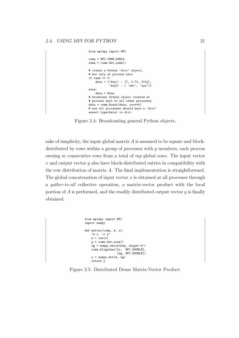
Figure 2.4 shows an example of high-level communication of Python ob-
jects. A Python dictionary created a process zero, next it is collectively broad-
cast to all other processes within a communicator.
An additional example of collective communication is shown in figure 2.5.
In this case, NumPy arrays are communicated by using their exposed memory
buffers, thus avoiding the overhead of serialization/deserialization steps. This
example implements a parallel dense matrix-vector product y = Ax. For the
2.4. USING MPI FOR PYTHON 21
from mpi4py import MPI
comm = MPI.COMM_WORLD
rank = comm.Get_rank()
# create a Python ’dict’ object,
# but only at process zero
if rank == 0:
data = ’key1’ : [7, 2.72, 2+3j],
’key2’ : ( ’abc’, ’xyz’)
else:
data = None
# broadcast Python object created at
# process zero to all other processes
data = comm.Bcast(data, root=0)
# now all processes should have a ’dict’
assert type(data) is dict
Figure 2.4: Broadcasting general Python objects.
sake of simplicity, the input global matrix A is assumed to be square and block-
distributed by rows within a group of processes with p members, each process
owning m consecutive rows from a total of mp global rows. The input vector
x and output vector y also have block-distributed entries in compatibility with
the row distribution of matrix A. The final implementation is straightforward.
The global concatenation of input vector x is obtained at all processes through
a gather-to-all collective operation, a matrix-vector product with the local
portion of A is performed, and the readily distributed output vector y is finally
obtained.
from mpi4py import MPI
import numpy
def matvec(comm, A, x):
"A x -> y"
m = len(x)
p = comm.Get_size()
xg = numpy.zeros(m*p, dtype=’d’)
comm.Allgather([x, MPI.DOUBLE],
[xg, MPI.DOUBLE])
y = numpy.dot(A, xg)
return y
Figure 2.5: Distributed Dense Matrix-Vector Product.

22 CHAPTER 2. MPI FOR PYTHON
2.4.2 Dynamic Process Management
In MPI for Python, new independent processes groups can be created by call-
ing the Spawn() method within an intracommunicator (i.e., an Intracomm
instance). This call returns a new intercommunicator (i.e., an Intercomm in-
stance) at the parent process group. The child process group can retrieve the
matching intercommunicator by calling the Get_parent() method defined in
the Comm class. At each side, the new intercommunicator can be used to per-
form point to point and collective communications between the parent and
child groups of processes.
Alternatively, disjoint groups of processes can establish communication
using a client/server approach. Any server application must first call the
Open_port() function to open a “port” and the Publish_name() function
to publish a provided “service”, and next call the Accept() method within
an Intracomm instance. Any client applications can first find a published
“service” by calling the Lookup_name() function, which returns the “port”
where a server can be contacted; and next call the Connect() method within
an Intracomm instance. Both Accept() and Connect() methods return an
Intercomm instance. When connection between client/server processes is no
longer needed, all of them must cooperatively call the Disconnect() method
of the Comm class. Additionally, server applications should release resources by
calling the Unpublish_name() and Close_port() functions.
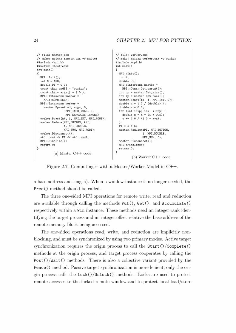
As an example, figures 2.6 and 2.7 show a Python and a C++ implemen-
tation of a master/worker approach for approximately computing the number
π in parallel through a simple numerical quadrature applied to the definite
integral∫ 1
04(1 + x2)−1dx.
The codes on the left (figures 2.6a and 2.7a) implement “master”, sequen-
tial applications. These master applications create a new group of independent
processes and communicate with them by sending (through a broadcast oper-
ation) and receiving (through a reduce operation) data. The codes on the
right (figures 2.6b and 2.7b) implement “worker”, parallel applications. These
worker applications are in charge of receiving input data from the master
(through a matching broadcast operation), making the actual computations,

2.4. USING MPI FOR PYTHON 23
and sending back the results (through a matching reduce operation).
A careful look at figures 2.6a and 2.7a reveals that, for each implemen-
tation language, the sequential master application spawns the worker appli-
cation implemented in the matching language. However, this setup can be
easily changed: the master application written in Python can stead spawn
the worker application written in C++; the master application written in
C++ can instead spawn the worker application written in Python. Thus
MPI for Python and its support for dynamic process management automat-
ically provides full interoperability with other codes using a master/worker
(or client/server) model, regardless of their specific implementation languages
being C, C++, or Fortran.
#! /usr/local/bin/python
# file: master.py
from mpi4py import MPI
from numpy import array
N = array(100, ’i’)
PI = array(0.0, ’d’)
cmd = ’worker.py’
args = []
master = MPI.COMM_SELF
worker = master.Spawn(cmd, args, 5)
worker.Bcast([N,MPI.INT], root=MPI.ROOT)
sbuf = None
rbuf = [PI, MPI.DOUBLE]
worker.Reduce(sbuf, rbuf,
op=MPI.SUM,
root=MPI.ROOT)
worker.Disconnect()
print PI
(a) Master Python code
#! /usr/local/bin/python
# file: worker.py
from mpi4py import MPI
from numpy import array
N = array(0, ’i’)
PI = array(0, ’d’)
master = MPI.Comm.Get_parent()
np = master.Get_size()
ip = master.Get_rank()
master.Bcast([N, MPI.INT], root=0)
h = 1.0 / N
s = 0.0
for i in xrange(ip, N, np):
x = h * (i + 0.5)
s += 4.0 / (1.0 + x**2)
PI[...] = s * h
sbuf = [PI, MPI.DOUBLE]
rbuf = None
master.Reduce(sbuf, rbuf,
op=MPI.SUM,
root=0)
master.Disconnect()
(b) Worker Python code
Figure 2.6: Computing π with a Master/Worker Model in Python.
2.4.3 One-sided Operations
In MPI for Python, one-sided operations are available by using instances of the
Win class. New window objects are created by calling the Create() method
at all processes within a communicator and specifying a memory buffer (i.e.,
24 CHAPTER 2. MPI FOR PYTHON
// file: master.cxx
// make: mpicxx master.cxx -o master
#include <mpi.h>
#include <iostream>
int main()
MPI::Init();
int N = 100;
double PI = 0.0;
const char cmd[] = "worker";
const char* args[] = 0 ;
MPI::Intracomm master =
MPI::COMM_SELF;
MPI::Intercomm worker =
master.Spawn(cmd, args, 5,
MPI_INFO_NULL, 0,
MPI_ERRCODES_IGNORE);
worker.Bcast(&N, 1, MPI_INT, MPI_ROOT);
worker.Reduce(MPI_BOTTOM, &PI,
1, MPI_DOUBLE,
MPI_SUM, MPI_ROOT);
worker.Disconnect();
std::cout << PI << std::endl;
MPI::Finalize();
return 0;
(a) Master C++ code
// file: worker.cxx
// make: mpicxx worker.cxx -o worker
#include <mpi.h>
int main()
MPI::Init();
int N;
double PI;
MPI::Intercomm master =
MPI::Comm::Get_parent();
int np = master.Get_size();
int ip = master.Get_rank();
master.Bcast(&N, 1, MPI_INT, 0);
double h = 1.0 / (double) N;
double s = 0.0;
for (int i=ip; i<N; i+=np)
double x = h * (i + 0.5);
s += 4.0 / (1.0 + x*x);
PI = s * h;
master.Reduce(&PI, MPI_BOTTOM,
1, MPI_DOUBLE,
MPI_SUM, 0);
master.Disconnect();
MPI::Finalize();
return 0;
(b) Worker C++ code
Figure 2.7: Computing π with a Master/Worker Model in C++.
a base address and length). When a window instance is no longer needed, the
Free() method should be called.
The three one-sided MPI operations for remote write, read and reduction
are available through calling the methods Put(), Get(), and Accumulate()
respectively within a Win instance. These methods need an integer rank iden-
tifying the target process and an integer offset relative the base address of the
remote memory block being accessed.
The one-sided operations read, write, and reduction are implicitly non-
blocking, and must be synchronized by using two primary modes. Active target
synchronization requires the origin process to call the Start()/Complete()
methods at the origin process, and target process cooperates by calling the
Post()/Wait() methods. There is also a collective variant provided by the
Fence() method. Passive target synchronization is more lenient, only the ori-
gin process calls the Lock()/Unlock() methods. Locks are used to protect
remote accesses to the locked remote window and to protect local load/store

2.4. USING MPI FOR PYTHON 25
accesses to a locked local window.
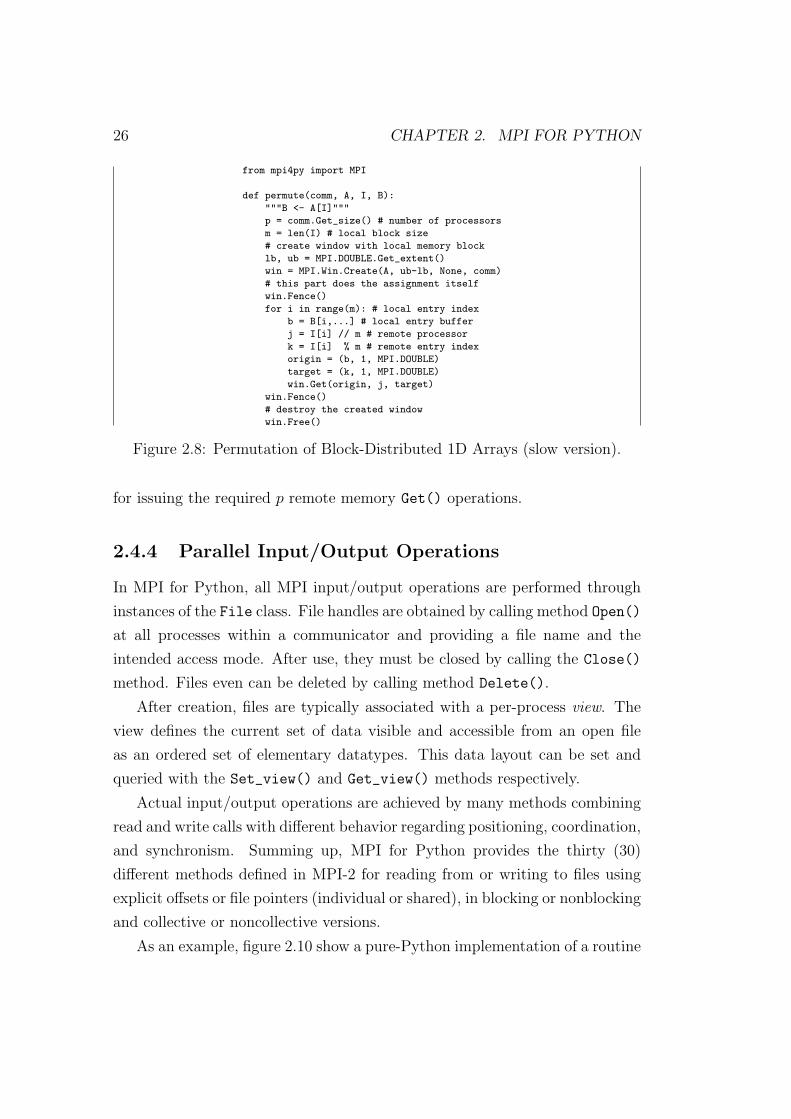
As an example, figures 2.8 and 2.9 show two possible implementations of a
parallel indirect assignment B = A(I), were A and B are two one-dimensional,
double precision floating point arrays and I is an integer permutation array.
For the sake of simplicity, A, B, and I are assumed to have the same block-
distribution with m local entries in p processes within a communicator.
In both implementations, a new window object is created by calling the
Create() method of the Win class. The window is constructed to make avail-
able the memory block of each local input array A at a group of processes
implicitly defined by a communicator. Additionally, a displacement unit equal
to the extent of the DOUBLE predefined datatype is specified; this extent is com-
puted from the lower bound and upper bound obtained through the method
Get_extent() of the Datatype class. The memory block of local output array
B is the destination of remote Get() operations; they are issued between a
couple of calls to the collective, barrier-like synchronization operation on the
window object through the Fence() method.
The simpler version shown in figure 2.8 is a pure-Python implementation.
It just computes the target process and the remote entry index for each needed
local entry, and issues a Get() call in order to obtain the corresponding local
value. As there are m remote memory accesses, this version is expected to be
slow for large arrays.
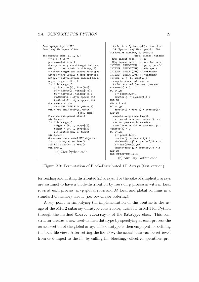
The more efficient but complex version shown in figure 2.9 is a mixed
Python-Fortran implementation. It requires only p remote memory accesses,
thus being expected to be faster than the previous version for larger arrays.
The auxiliary Fortran code shown in figure 2.9a implements a helper routine
in charge of computing the index mapping associating needed local entries to
remote entries at each process. This routine is made available to Python by
using F2PY interface generator.
The core Python code shown in figure 2.9b employs the output of the helper
Fortran routine for constructing user-defined MPI datatypes. Those datatypes
are created through the constructor method Create_indexed_block() of the
Datatype class; they contain the required information in order to access local
and remote array entries. Finally, those used-defined datatypes are employed
26 CHAPTER 2. MPI FOR PYTHON
from mpi4py import MPI
def permute(comm, A, I, B):
"""B <- A[I]"""
p = comm.Get_size() # number of processors
m = len(I) # local block size
# create window with local memory block
lb, ub = MPI.DOUBLE.Get_extent()
win = MPI.Win.Create(A, ub-lb, None, comm)
# this part does the assignment itself
win.Fence()
for i in range(m): # local entry index
b = B[i,...] # local entry buffer
j = I[i] // m # remote processor
k = I[i] % m # remote entry index
origin = (b, 1, MPI.DOUBLE)
target = (k, 1, MPI.DOUBLE)
win.Get(origin, j, target)
win.Fence()
# destroy the created window
win.Free()
Figure 2.8: Permutation of Block-Distributed 1D Arrays (slow version).
for issuing the required p remote memory Get() operations.
2.4.4 Parallel Input/Output Operations
In MPI for Python, all MPI input/output operations are performed through
instances of the File class. File handles are obtained by calling method Open()
at all processes within a communicator and providing a file name and the
intended access mode. After use, they must be closed by calling the Close()
method. Files even can be deleted by calling method Delete().
After creation, files are typically associated with a per-process view. The
view defines the current set of data visible and accessible from an open file
as an ordered set of elementary datatypes. This data layout can be set and
queried with the Set_view() and Get_view() methods respectively.
Actual input/output operations are achieved by many methods combining
read and write calls with different behavior regarding positioning, coordination,
and synchronism. Summing up, MPI for Python provides the thirty (30)
different methods defined in MPI-2 for reading from or writing to files using
explicit offsets or file pointers (individual or shared), in blocking or nonblocking
and collective or noncollective versions.
As an example, figure 2.10 show a pure-Python implementation of a routine
2.4. USING MPI FOR PYTHON 27
from mpi4py import MPI
from pmaplib import mkidx
def permute(comm, A, I, B):
"""B <- A[I]"""
p = comm.Get_size()
# compute origin and target indices
dist, oindex, tindex = mkidx(p, I)
# create origin and target datatypes
abtype = MPI.DOUBLE # base datatype
mktype = abtype.Create_indexed_block
otype, ttype = [], []
for i in range(p):
j, k = dist[i], dist[i+1]
ot = mktype(1, oindex[j:k])
tt = mktype(1, tindex[j:k])
ot.Commit(); otype.append(ot)
tt.Commit(); ttype.append(tt)
# create a window
lb, ub = MPI.DOUBLE.Get_extent()
win = MPI.Win.Create(A, ub-lb,
None, comm)
# do the assignment itself
win.Fence()
for i in range(p):
origin = (B, 1, otype[i])
target = (0, 1, ttype[i])
win.Get(origin, i, target)
win.Fence()
# destroy the created MPI objects
for ot in otype: ot.Free()
for tt in ttype: tt.Free()
win.Free()
(a) Core Python code
! to build a Python module, use this:
! $$ f2py -m pmaplib -c pmaplib.f90
SUBROUTINE mkidx(p, m, perm, &
dist, oindex, tindex)
!f2py intent(hide) :: m
!f2py depend(perm) :: m = len(perm)
INTEGER, INTENT(IN) :: p, m, perm(m)
INTEGER, INTENT(OUT) :: dist(p+1)
INTEGER, INTENT(OUT) :: oindex(m)
INTEGER, INTENT(OUT) :: tindex(m)
INTEGER i, j, k, counter(p)
! compute number of entries
! to be received from each process
counter(:) = 0
DO i=1,m
j = perm(i)/m+1
counter(j) = counter(j)+1
END DO
dist(1) = 0
DO i=1,p
dist(i+1) = dist(i) + counter(i)
END DO
! compute origin and target
! indices of entries; entry ’i’ at
! current process is received
! from location ’k’ at process ’j’.
counter(:) = 0
DO i=1,m
j = perm(i)/m+1
counter(j) = counter(j)+1
oindex(dist(j) + counter(j)) = i-1
k = MOD(perm(i),m)
tindex(dist(j) + counter(j)) = k
END DO
END SUBROUTINE mkidx
(b) Auxiliary Fortran code
Figure 2.9: Permutation of Block-Distributed 1D Arrays (fast version).
for reading and writing distributed 2D arrays. For the sake of simplicity, arrays
are assumed to have a block-distribution by rows on p processes with m local
rows at each process, m · p global rows and M local and global columns in a
standard C memory layout (i.e. row-major ordering).
A key point in simplifying the implementation of this routine is the us-
age of the MPI-2 subarray datatype constructor, available in MPI for Python
through the method Create_subarray() of the Datatype class. This con-
structor creates a new used-defined datatype by specifying at each process the
owned section of the global array. This datatype is then employed for defining
the local file view. After setting the file view, the actual data can be retrieved
from or dumped to the file by calling the blocking, collective operations pro-

28 CHAPTER 2. MPI FOR PYTHON
vided by the Read_all() or Write_all() methods.
from mpi4py import MPI
def arrayio(op, A, atype, filename, comm):
# create datatype for setting the file view on
# this process; global array has dimensions (M,M),
# all local arrays have local dimension (m,M).
rank = comm.Get_rank()
m, M = A.shape
sizes = [M, M] # global array shape
subsizes = [m, M] # local subarray shape
starts = [m*rank, 0] # start of section here
order = MPI.ORDER_C # ie. row major order
mktype = atype.Create_subarray # constructor
view = mktype(sizes, subsizes, starts, order)
# open file for reading or writing,
# additionally, set file view datatype
if op == ’r’:
mode = MPI.MODE_RDONLY
elif op == ’w’:
mode = MPI.MODE_WRONLY | MPI.MODE_CREATE
fh = MPI.File.Open(comm, filename, mode)
fh.Set_view(etype=atype, filetype=view)
# read or write data
if op == ’r’:
fh.Read_all([A, atype])
elif op == ’w’:
fh.Write_all([A, atype])
# close opened file, free view datatype
fh.Close()
view.Free()
def read(A, atype, filename, comm):
arrayio(’r’, A, atype, filename, comm)
def write(A, atype, filename, comm):
arrayio(’w’, A, atype, filename, comm)
Figure 2.10: Input/Output of Block-Distributed 2D Arrays.
2.5 Efficiency Tests
Some efficiency tests were run on the Beowulf class cluster Aquiles [34]. Its
hardware consists of eighty disk-less single processor computing nodes with
Intel Pentium 4 Prescott 3.0GHz 2MB cache processors, Intel Desktop Board
D915PGN motherboards, Kingston Value RAM 2GB DDR 400MHz memory,
and 3Com 2000ct Gigabit LAN network cards, interconnected with a 3Com
SuperStack 3 Switch 3870 48-ports Gigabit Ethernet.
MPI for Python was built on a Linux 2.6.17 box using GCC 3.4.6 compiler
2.5. EFFICIENCY TESTS 29
with Python 2.5.1. The chosen MPI implementation was MPICH2 1.0.5p4.
Communications between processes involved numeric arrays, they were pro-
vided by NumPy 1.0.3.
2.5.1 Measuring Overhead in Message Passing Opera-
tions
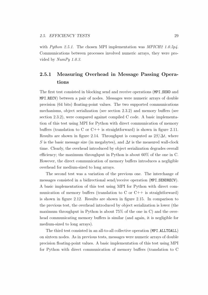
The first test consisted in blocking send and receive operations (MPI SEND and
MPI RECV) between a pair of nodes. Messages were numeric arrays of double
precision (64 bits) floating-point values. The two supported communications
mechanisms, object serialization (see section 2.3.2) and memory buffers (see
section 2.3.2), were compared against compiled C code. A basic implementa-
tion of this test using MPI for Python with direct communication of memory
buffers (translation to C or C++ is straightforward) is shown in figure 2.11.
Results are shown in figure 2.14. Throughput is computed as 2S/∆t, where
S is the basic message size (in megabytes), and ∆t is the measured wall-clock
time. Clearly, the overhead introduced by object serialization degrades overall
efficiency; the maximum throughput in Python is about 60% of the one in C.
However, the direct communication of memory buffers introduces a negligible
overhead for medium-sized to long arrays.
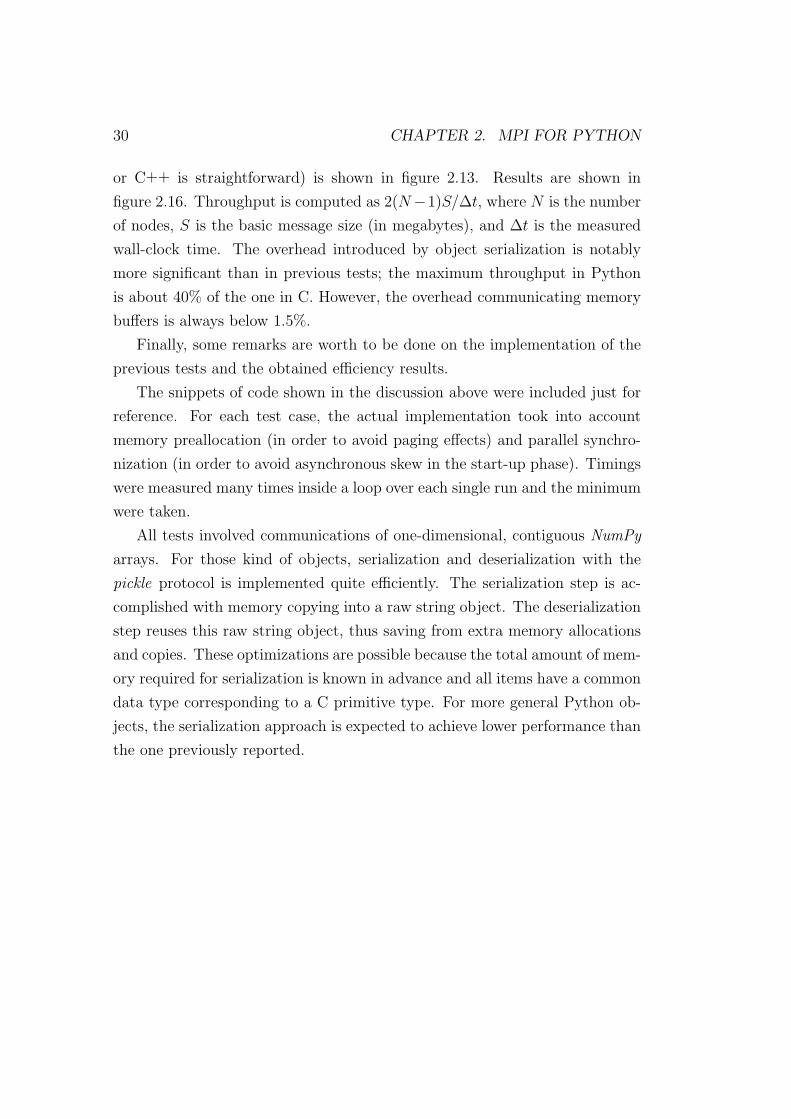
The second test was a variation of the previous one. The interchange of
messages consisted in a bidirectional send/receive operation (MPI SENDRECV).
A basic implementation of this test using MPI for Python with direct com-
munication of memory buffers (translation to C or C++ is straightforward)
is shown in figure 2.12. Results are shown in figure 2.15. In comparison to
the previous test, the overhead introduced by object serialization is lower (the
maximum throughput in Python is about 75% of the one in C) and the over-
head communicating memory buffers is similar (and again, it is negligible for
medium-sized to long arrays).
The third test consisted in an all-to-all collective operation (MPI ALLTOALL)
on sixteen nodes. As in previous tests, messages were numeric arrays of double
precision floating-point values. A basic implementation of this test using MPI
for Python with direct communication of memory buffers (translation to C
30 CHAPTER 2. MPI FOR PYTHON
or C++ is straightforward) is shown in figure 2.13. Results are shown in
figure 2.16. Throughput is computed as 2(N−1)S/∆t, where N is the number
of nodes, S is the basic message size (in megabytes), and ∆t is the measured
wall-clock time. The overhead introduced by object serialization is notably
more significant than in previous tests; the maximum throughput in Python
is about 40% of the one in C. However, the overhead communicating memory
buffers is always below 1.5%.
Finally, some remarks are worth to be done on the implementation of the
previous tests and the obtained efficiency results.
The snippets of code shown in the discussion above were included just for
reference. For each test case, the actual implementation took into account
memory preallocation (in order to avoid paging effects) and parallel synchro-
nization (in order to avoid asynchronous skew in the start-up phase). Timings
were measured many times inside a loop over each single run and the minimum
were taken.
All tests involved communications of one-dimensional, contiguous NumPy
arrays. For those kind of objects, serialization and deserialization with the
pickle protocol is implemented quite efficiently. The serialization step is ac-
complished with memory copying into a raw string object. The deserialization
step reuses this raw string object, thus saving from extra memory allocations
and copies. These optimizations are possible because the total amount of mem-
ory required for serialization is known in advance and all items have a common
data type corresponding to a C primitive type. For more general Python ob-
jects, the serialization approach is expected to achieve lower performance than
the one previously reported.
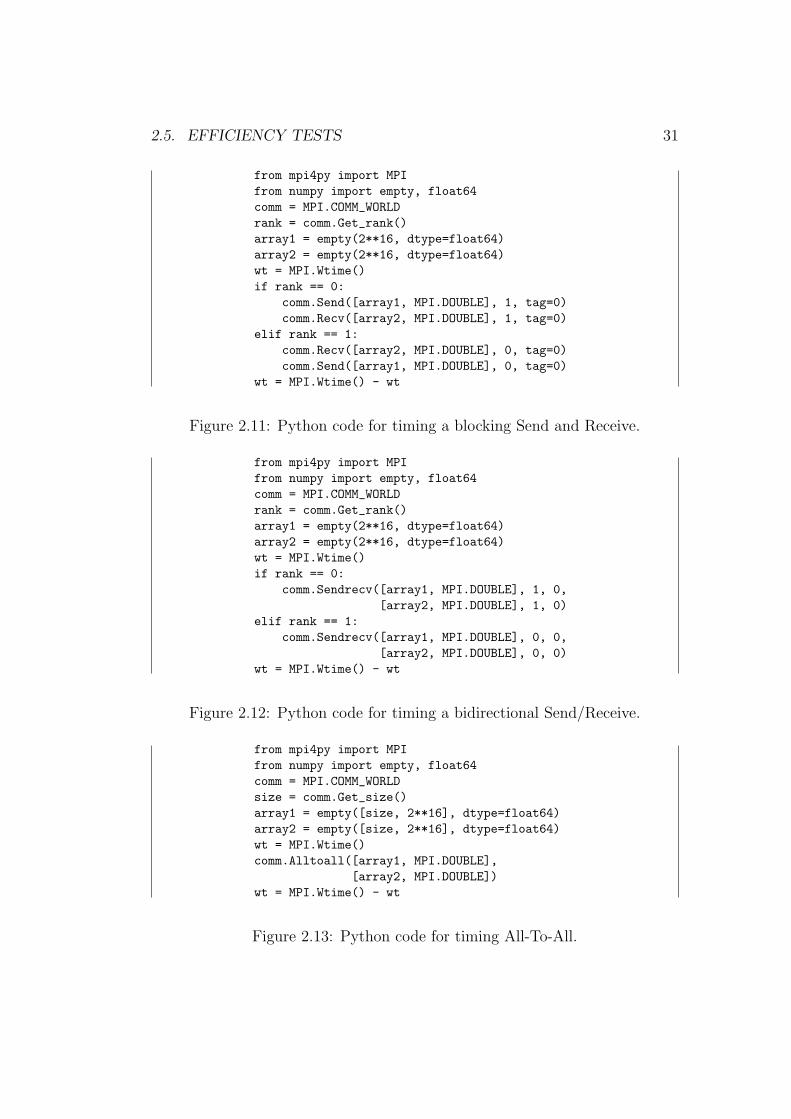
2.5. EFFICIENCY TESTS 31
from mpi4py import MPIfrom numpy import empty, float64comm = MPI.COMM_WORLDrank = comm.Get_rank()array1 = empty(2**16, dtype=float64)array2 = empty(2**16, dtype=float64)wt = MPI.Wtime()if rank == 0:
comm.Send([array1, MPI.DOUBLE], 1, tag=0)comm.Recv([array2, MPI.DOUBLE], 1, tag=0)
elif rank == 1:comm.Recv([array2, MPI.DOUBLE], 0, tag=0)comm.Send([array1, MPI.DOUBLE], 0, tag=0)
wt = MPI.Wtime() - wt
Figure 2.11: Python code for timing a blocking Send and Receive.
from mpi4py import MPIfrom numpy import empty, float64comm = MPI.COMM_WORLDrank = comm.Get_rank()array1 = empty(2**16, dtype=float64)array2 = empty(2**16, dtype=float64)wt = MPI.Wtime()if rank == 0:
comm.Sendrecv([array1, MPI.DOUBLE], 1, 0,[array2, MPI.DOUBLE], 1, 0)
elif rank == 1:comm.Sendrecv([array1, MPI.DOUBLE], 0, 0,
[array2, MPI.DOUBLE], 0, 0)wt = MPI.Wtime() - wt
Figure 2.12: Python code for timing a bidirectional Send/Receive.
from mpi4py import MPIfrom numpy import empty, float64comm = MPI.COMM_WORLDsize = comm.Get_size()array1 = empty([size, 2**16], dtype=float64)array2 = empty([size, 2**16], dtype=float64)wt = MPI.Wtime()comm.Alltoall([array1, MPI.DOUBLE],
[array2, MPI.DOUBLE])wt = MPI.Wtime() - wt
Figure 2.13: Python code for timing All-To-All.
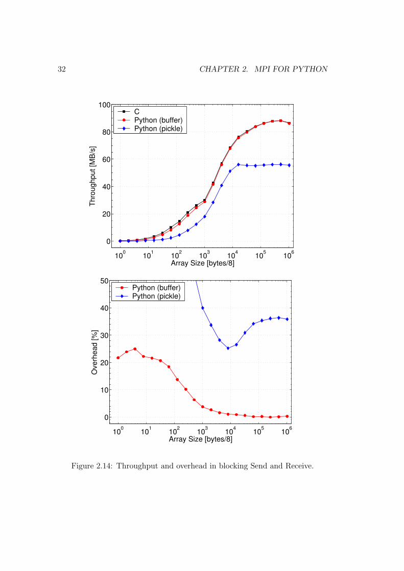
32 CHAPTER 2. MPI FOR PYTHON
100
101
102
103
104
105
106
0
20
40
60
80
100
Array Size [bytes/8]
Thro
ughp
ut [M
B/s
]
CPython (buffer)Python (pickle)
100
101
102
103
104
105
106
0
10
20
30
40
50
Array Size [bytes/8]
Ove
rhea
d [%
]
Python (buffer)Python (pickle)
Figure 2.14: Throughput and overhead in blocking Send and Receive.

2.5. EFFICIENCY TESTS 33
100
101
102
103
104
105
106
0
20
40
60
80
100
Array Size [bytes/8]
Thro
ughp
ut [M
B/s
]CPython (buffer)Python (pickle)
100
101
102
103
104
105
106
0
10
20
30
40
50
Array Size [bytes/8]
Ove
rhea
d [%
]
Python (buffer)Python (pickle)
Figure 2.15: Throughput and overhead in bidirectional Send/Receive.

34 CHAPTER 2. MPI FOR PYTHON
105
106
0
20
40
60
80
100
Array Size [bytes/8]
Thro
ughp
ut [M
B/s
] CPython (buffer)Python (pickle)
105
106
0
0.5
1
1.5
2
Array Size [bytes/8]
Ove
rhea
d [%
]
Python (buffer)
Figure 2.16: Throughput and overhead in All-To-All.

2.5. EFFICIENCY TESTS 35
2.5.2 Comparing Wall-Clock Timings for Collective
Communication Operations
Additional efficiency tests were run on the older Beowulf class cluster Geron-
imo [35]. Hardware consisted of ten computing nodes with Intel P4 2.4Ghz
processors, 512KB cache size, 1024MB RAM DDR 333MHz and 3COM 3c509
(Vortex) Nic cards interconnected with an Encore ENH924-AUT+ 100Mbps
Fast Ethernet switch.
Those tests consisted in wall-clock time measurements of some collective
operations on ten uniprocessor nodes. Messages were again numeric arrays of
double precision floating-point values. Results are shown in figures 2.17 to 2.21.
For array sizes greater than 103 (8KB), timings in Python are between 5% (for
broadcast) to 20% (for all-to-all) greater than timings in C.
101
102
103
104
105
10610
−5
10−4
10−3
10−2
10−1
100
101
Array Size [bytes/8]
Tim
e [s
ecs]
CPython
Figure 2.17: Timing in Broadcast.

36 CHAPTER 2. MPI FOR PYTHON
101
102
103
104
105
10610
−5
10−4
10−3
10−2
10−1
100
101
Array Size [bytes/8]
Tim
e [s
ecs]
CPython
Figure 2.18: Timing in Scatter.
101
102
103
104
105
10610
−6
10−4
10−2
100
102
Array Size [bytes/8]
Tim
e [s
ecs]
CPython
Figure 2.19: Timing in Gather.

2.5. EFFICIENCY TESTS 37
101
102
103
104
105
10610
−4
10−3
10−2
10−1
100
101
102
Array Size [bytes/8]
Tim
e [s
ecs]
CPython
Figure 2.20: Timing in Gather to All.
101
102
103
104
105
10610
−4
10−3
10−2
10−1
100
101
102
Array Size [bytes/8]
Tim
e [s
ecs]
CPython
Figure 2.21: Timing in All to All Scatter/Gather.


Chapter 3
PETSc for Python
This chapter is devoted to describing PETSc for Python, an open-source,
public-domain software project that provides access to the Portable, Extensible
Toolkit for Scientific Computation (PETSc) libraries for the Python program-
ming language.
PETSc for Python is a general-purpose and full-featured package. Its facili-
ties allow sequential and parallel Python applications to exploit state of the art
algorithms and data structures readily implemented in PETSc and targeted
to large-scale numerical simulations arising in many problems of science and
engineering.
Section 3.1 presents a general description about PETSc and their main
components and features. Section 3.2 describes the general design and imple-
mentation of PETSc for Python through a mixed language, C-Python approach
and the help of the SWIG interface generator.
Section 3.3 presents a general overview of the many PETSc concepts and
functionalities accessible through PETSc for Python. Additionally, a series of
short, self-contained example codes with their corresponding discussions is pro-
vided. These examples show how to use PETSc for Python for implementing
sequential and parallel Python codes with the help of PETSc.
Finally, section 3.4 presents some efficiency tests and discusses their results.
Those test are focused on determining the calling overhead introduced by the
Python layer. This is done by measuring and comparing wall clock timings of
39
40 CHAPTER 3. PETSC FOR PYTHON
a simple sequential application implemented both in C and Python and some
auxiliary Fortran code. The application is related to the numerical solution of a
model linear boundary value problem using matrix-free techniques and Krylov-
based iterative methods for solving the subsidiary linear systems arising from
a finite differences discretization.
3.1 An Overview of PETSc
PETSc [2, 4], the Portable Extensible Toolkit for Scientific Computation, is a
suite of algorithms and data structures for the solution of problems arising on
scientific and engineering applications, specially those modeled by partial dif-
ferential equations, of large-scale nature, and targeted for parallel, distributed-
memory computing environments [5].
PETSc is written in C (thus making it usable from C++); a Fortran inter-
face (very similar to the C one) is also available. The complete set of features
provided by PETSc is better exploited when it is employed for implementing
parallel applications. Nevertheless, PETSc perfectly supports the implemen-
tation of sequential applications.
PETSc employs the MPI standard for inter-process communication, thus
it is based on the message-passing model for parallel computing. Despite this,
PETSc provides many high-level functionalities that typical users needs to
write very few message-passing calls on their specific codes.
Being written in C and based on MPI, PETSc is highly portable soft-
ware library. PETSc-based applications can run in almost all modern parallel
environment, ranging from distributed memory architectures (with standard
networks as well as specialized communication hardware) to multi-processor
(and multi-core) shared memory machines.
3.1.1 Main Features of PETSc
PETSc is designed with an object-oriented style. Almost all user-level objects
are instances of some specific type. Those objects are managed through handles
to opaque data structures which are created, accessed and destroyed by calling

3.1. AN OVERVIEW OF PETSC 41
appropriate library routines. Additionally, PETSc is designed to be highly
modular: all of its abstractions are grouped into independent but interoperable
library components. Furthermore, this modular design enables PETSc to be
easily extended with several specialized parallel libraries like HYPRE [36],
Trilinos/ML [37], MUMPS [38], SPAI [39], and others through an unified
interface.
Vectors
The Vec component of PETSc provides the basic data structure for storing
right-hand sides and solutions of linear and nonlinear systems of equations,
representing finite-dimensional elements or vector subspaces, etc. More par-
ticularly, they are employed to store field data on nodes and cells of compu-
tational grids associated to the discretization of partial differential equations.
For those kind of applications, PETSc also provides additional components
like index sets and general vector scatter/gather operations. In the parallel
case, those abstraction encapsulate and simplify message passing of field data.
PETSc provides two basic vector types: sequential and parallel. Sequential
vectors store their entries in a contiguous array. Parallel vectors are partitioned
across processes: each process owns an arbitrary length but contiguous range
of the entries, which are again stored in local contiguous arrays.
Regardless of their specific type, vectors are managed through a unified
interface which provide access to many common operation like dot products,
computing of norms, linear combinations, point-wise operations, etc.. In the
parallel case, inserting or adding values to vector entries is a simple, high-
level operation: in a first step, any process can set any component of the
global vector; in a second step, PETSc insures that non-local components are
automatically stored in the correct location by performing any needed message
passing.
Matrices
The Mat component of PETSc provides a large suite of routines and data
structures for the efficient manipulation of matrices. PETSc provides a variety
42 CHAPTER 3. PETSC FOR PYTHON
of matrix implementations, ranging from dense to sparse, because no single
matrix format is appropriate for all problems. Almost all of them are available
in both sequential and parallel version.
Dense matrices store all their entries in a logically two-dimensional, column-
major, contiguous array (as in the usual Fortran ordering). In the parallel case,
dense matrices are row-partitioned, and each process owns an arbitrary length
but contiguous range of the rows. At each process, those rows are stored in a
sequential dense matrix.
Sparse matrices store only non-zero entries using many specialized formats.
The default, simplest and more commonly used matrix implementation is the
general sparse AIJ format (also known as the Yale sparse matrix format or
compressed sparse row format, CSR). In the parallel case, sparse matrices are
row-partitioned, and each process owns an arbitrary length but contiguous
range of the rows. In order to efficiently implement the parallel matrix-vector
product operation, the set of rows at each processor is stored in two sequential
matrices: the diagonal part and the off-diagonal part. For a square global
matrix, the diagonal portion is a a square sub-matrix defined by it its local
rows and the corresponding columns, and the off-diagonal portion encompasses
the remainder of the local matrix entries (thus being in general a rectangular
sub-matrix).
Regardless of their specific type, matrices are managed through a unified
interface which provide access to many common operations like matrix-matrix
product, sub-matrix extraction, and matrix-vector product (a key operation
for the implementation or iterative methods). In the parallel case, inserting
or adding values to matrix entries is a simple, high-level operation: in a first
step, any process can set any component of the global matrix; in a second
step, PETSc insures that non-local components are automatically stored in
the correct location by performing any needed message passing.
Linear Solvers
The combination of Krylov methods and preconditioning strategies is at the
core of most modern numerical methods for the iterative solution of linear

3.1. AN OVERVIEW OF PETSC 43
system of equations. These problems have the general form
Ax = b,
where A denotes a non-singular linear operator, b is the right-hand-side vector,
and x is the solution vector.
Iterative linear solvers and preconditioners are a key part of PETSc. All the
provided functionalities are available through two independent but tightly con-
nected, interoperable components. The KSP component provides implementa-
tions of many popular Krylov subspace iterative methods; the PC component
includes a variety of preconditioners and direct (i.e., factorization-based) solu-
tion methods.
The KSP and PC abstractions provide efficient access and unified inter-
face in the sequential and parallel cases, for both iterative and direct solution
methods. In addition, users can easily customize the linear solvers, being able
to set the various tolerances, algorithmic parameters, and even define custom
routines for monitoring the solution process and declaring convergence.
Nonlinear Solvers
The SNES component of PETSc provides methods for solving systems of non-
linear equations of the form
F (x) = 0,
where F : <n → <n. Newton-like methods provide the core of the package,
including both line search and trust region techniques to ensure global conver-
gence to the solution. The general form of the n-dimensional Newton’s method
is
xk+1 = xk − [F ′(xk)]−1F (xk), k = 0, 1, . . . ,
where x0 is an initial approximation to the solution and F ′(xk), the Jaco-
bian, is non-singular at each iteration. In practice, the Newton iteration is

44 CHAPTER 3. PETSC FOR PYTHON
implemented by the following two steps:
1. (Approximately) solve F ′(xk)∆xk = −F (xk).
2. Update xk+1 = xk + ∆xk.
The interfaces to the various solvers are all virtually identical, even in the
parallel case; the only difference in the parallel version is that each process
typically forms only its local contribution to the function vector F and the
Jacobian matrix F ′. In addition, users can easily customize the nonlinear
solvers for the problem at hand. They are able to set the various tolerances,
algorithmic parameters, and even define routines for monitoring and declaring
convergence, thus having full control of the complete solution process.
PETSc nonlinear solvers can be used in conjunction with matrix-free tech-
niques. In the context of solving nonlinear problem, matrix-free approaches
take advantage of a combination of Newton-Krylov iterative methods. The
use of Krylov-based inner linear solver within the outer Newton iteration is
a crucial ingredient. Krylov methods do not require to access matrix entries.
Instead, they are formulated in terms of the action of a linear operator on a
given input vector. Then, the Jacobian do not have to be explicitly assembled
by user-provided code on a matrix data structure, nor matrix entries have to
be ever computed in any way (as is however the case if automatic differentia-
tion or colored finite differences techniques are employed). Instead, the action
of the Jacobian F ′(x) on a given vector v is internally approximated with the
following fist-order finite differences formula,
F ′(xk)v ≈F (xk + hv)− F (xk)
h
were h is an appropriately chosen scalar value [40, 41]. Then, the nonlinear
residual function is the only required input from the application side. In order
to compute an approximation to F ′(xk)v, only one evaluation of the user-
provided function F is required.

3.2. DESIGN AND IMPLEMENTATION 45
Time-steppers
The TS component of PETSc provides a framework for the scalable solu-
tion of ordinary differential equations arising from the discretization of time-
dependent partial differential equations. In addition, it provides some pseudo-
transient continuation techniques for computing steady-state solutions.
3.2 Design and Implementation
In the low-level layer, an extension module written in C provide access to
all functions and predefined constants in PETSc. Additionally, this C code
implements some core machinery for converting any PETSc object between
its Python representation (i.e. an instance of a specific Python class) and C
representation (i.e. an opaque PETSc object). All this conversion machinery
is carefully designed for supporting full interoperability between the C and
Python sides.
The approach described in the above paragraph is very similar to the one
previously described in section 2.3. However, as the number of user-level rou-
tines available in PETSc is huge, PETSc for Python took advantage of SWIG
(see section 1.2.4) in order to automate the generation of code connecting the
C and Python sides. Furthermore, this higly interoperable C-Python interface
supported on SWIG motivated other interesting developments; they are briefly
commented in chapter 5, near the end of section 5.1.
In the high-level layer, a series of modules written in Python define all class
hierarchies, methods and functions. This Python code is supported by the
low-level C extension module commented above. The final user interface has
some connections with the one in PETSc. However, the PETSc user interfaces
are not truly object-oriented; those languages do not natively support some
more advanced concepts such as classes, inheritance and polymorphism, or
exception-based error checking.
The user interface provided by PETSc for Python is a truly object oriented
and high-level one, being by far easier and pleasant to use than the native C
and Fortran ones provided in PETSc. Readers with some basic to serious
46 CHAPTER 3. PETSC FOR PYTHON
experience on programming with PETSc will hopefully realize this fact in the
following section.
3.3 Using PETSc for Python
This section presents a general overview and some examples of the many
PETSc functionalities readily available in PETSc for Python. The provided
examples are simple, self-contained, and implemented in a few lines of Python
code. Nevertheless, they show general usage patterns of PETSc for Python for
implementing linear algebra algorithms, assembling sparse matrices, and solv-
ing linear and nonlinear systems of equations within a Python programming
environment.
3.3.1 Working with Vectors
PETSc for Python provides access to PETSc vectors, index sets and general
vector scatter/gather operations through the Vec, IS, and Scatter classes
respectively. By using them, the management of distributed field data is highly
simplified in parallel applications.
Besides the use as containers for field data, PETSc vectors also represent
algebraic entities of finite-dimensional vector spaces. For this case, the Vec
class provides many methods for performing common linear algebra operations,
like computing vector updates (axpy(), aypx(), scale()), inner products
(dot()) and different kinds of norms (norm()).
Figure 3.1 shows a basic implementation of a Krylov-based iterative linear
solver, the (unpreconditioned) conjugate gradient method.
3.3.2 Working with Matrices
PETSc for Python provides access to PETSc matrices through the Mat class.
New Mat instances are obtained by calling the create() method. Next,
the user have to specify the row and column sizes by calling the setSizes()
method. Finally, a call to the setType() method select a particular matrix
implementation.

3.3. USING PETSC FOR PYTHON 47
cg(A, x, b, imax, ε) :i ⇐ 0r ⇐ b−Ax
d ⇐ r
δ0 ⇐ rT r
δ ⇐ δ0
while i < imax and
δ > δ0ε2 do :
q ⇐ Ad
α ⇐ δ
dT q
x ⇐ x + αd
r ⇐ r − αq
δold ⇐ δ
δ ⇐ rT r
β ⇐ δ
δold
d ⇐ r + βd
i ⇐ i + 1
(a) Algorithm
def cg(A, b, x, imax=50, eps=1e-6):
"""
A, b, x : matrix, rhs, solution
imax : maximum allowed iterations
eps : tolerance for convergence
"""
# allocate work vectors
r = b.duplicate()
d = b.duplicate()
q = b.duplicate()
# initialization
i = 0
A.mult(x, r)
r.aypx(-1, b)
r.copy(d)
delta_0 = r.dot(r)
delta = delta_0
# enter iteration loop
while i < imax and \
delta > delta_0 * eps**2:
A.mult(d, q)
alpha = delta / d.dot(q)
x.axpy(+alpha, d)
r.axpy(-alpha, q)
delta_old = delta
delta = r.dot(r)
beta = delta / delta_old
d.aypx(beta, r)
i = i + 1
return i, delta**0.5
(b) Implementation
Figure 3.1: Basic Implementation of Conjugate Gradient Method.
Matrix entries can be set (or added to existing entries) by calling the
setValues() method. PETSc simplifies the assembling of parallel matri-
ces. Any process can contribute to any entry. However, off-process entries
are internally cached. Because of this, a final call to the assemblyBegin()
and assemblyEnd() methods is required in order to communicate off-process
entries to the actual owning process. Additionally, those calls prepare some
internal data structures for performing efficient parallel operations like matrix-
vector product. The later operation is available by calling the mult() method.
Figure 3.2 shows the basic steps for creating and assembling a sparse ma-
trix in parallel. The assembled matrix is a discrete representation of the two-
dimensional Laplace operator on the unit square equipped with homogeneous
boundary conditions after a 5-points finite differences discretization. The grid

48 CHAPTER 3. PETSC FOR PYTHON
supporting the discretization scheme is structured and regularly spaced. Fur-
thermore, the grid nodes have a simple contiguous block-distribution by rows
on a group of processes.
from petsc4py import PETSc
# grid size and spacing
m, n = 32, 32
hx = 1.0/(m-1)
hy = 1.0/(n-1)
# create sparse matrix
A = PETSc.Mat()
A.create(PETSc.COMM_WORLD)
A.setSizes([m*n, m*n])
A.setType(’aij’) # sparse
# precompute values for setting
# diagonal and non-diagonal entries
diagv = 2.0/hx**2 + 2.0/hy**2
offdx = -1.0/hx**2
offdy = -1.0/hy**2
# loop over owned block of rows on this
# processor and insert entry values
Istart, Iend = A.getOwnershipRange()
for I in xrange(Istart, Iend) :
A[I,I] = diagv
i = I//n # map row number to
j = I - i*n # grid coordinates
if i> 0 : J = I-n; A[I,J] = offdx
if i< m-1: J = I+n; A[I,J] = offdx
if j> 0 : J = I-1; A[I,J] = offdy
if j< n-1: J = I+1; A[I,J] = offdy
# communicate off-processor values
# and setup internal data structures
# for performing parallel operations
A.assemblyBegin()
A.assemblyEnd()
Figure 3.2: Assembling a Sparse Matrix in Parallel.
3.3.3 Using Linear Solvers
PETSc for Python provides access to PETSc linear solvers and preconditioners
through the KSP and PC classes.
New KSP instances are obtained by calling the create() method; this call
also creates automatically a companion inner preconditioner that can be re-
trieved with the getPC() method for further manipulations. The KSP and
PC classes provide the setType() methods for the selection of a specific it-
erative method and preconditioning strategy. The setTolerances() method
enable the specification of the different tolerances for declaring convergence;
other algorithmic parameters can also be set. Additionally, PETSc for Python
supports attaching user-defined Python function for monitoring the iterative
process (by calling the setMonitor() method) and even define a custom con-
vergence criteria (by calling the setConvergenceTest() method).
KSP objects have to be associated with a matrix (i.e., a Mat instance) rep-
resenting the operator of the linear problem and a (possibly different) matrix
for defining the preconditioner. This is done by calling the setOperators()
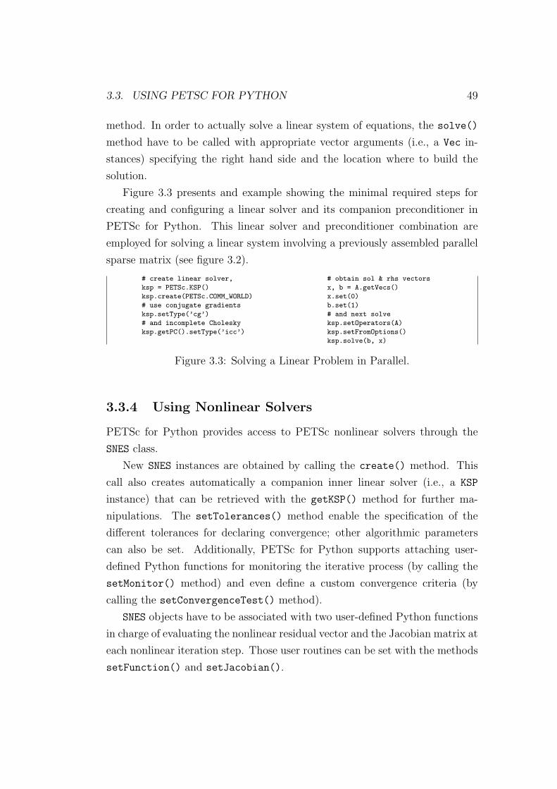
3.3. USING PETSC FOR PYTHON 49
method. In order to actually solve a linear system of equations, the solve()
method have to be called with appropriate vector arguments (i.e., a Vec in-
stances) specifying the right hand side and the location where to build the
solution.
Figure 3.3 presents and example showing the minimal required steps for
creating and configuring a linear solver and its companion preconditioner in
PETSc for Python. This linear solver and preconditioner combination are
employed for solving a linear system involving a previously assembled parallel
sparse matrix (see figure 3.2).
# create linear solver,
ksp = PETSc.KSP()
ksp.create(PETSc.COMM_WORLD)
# use conjugate gradients
ksp.setType(’cg’)
# and incomplete Cholesky
ksp.getPC().setType(’icc’)
# obtain sol & rhs vectors
x, b = A.getVecs()
x.set(0)
b.set(1)
# and next solve
ksp.setOperators(A)
ksp.setFromOptions()
ksp.solve(b, x)
Figure 3.3: Solving a Linear Problem in Parallel.
3.3.4 Using Nonlinear Solvers
PETSc for Python provides access to PETSc nonlinear solvers through the
SNES class.
New SNES instances are obtained by calling the create() method. This
call also creates automatically a companion inner linear solver (i.e., a KSP
instance) that can be retrieved with the getKSP() method for further ma-
nipulations. The setTolerances() method enable the specification of the
different tolerances for declaring convergence; other algorithmic parameters
can also be set. Additionally, PETSc for Python supports attaching user-
defined Python functions for monitoring the iterative process (by calling the
setMonitor() method) and even define a custom convergence criteria (by
calling the setConvergenceTest() method).
SNES objects have to be associated with two user-defined Python functions
in charge of evaluating the nonlinear residual vector and the Jacobian matrix at
each nonlinear iteration step. Those user routines can be set with the methods
setFunction() and setJacobian().

50 CHAPTER 3. PETSC FOR PYTHON
In order to actually solve a nonlinear system of equations, the solve()
method have to be called with appropriate vector arguments (i.e., a Vec in-
stances) specifying an optional right hand side (usually not provided as it is the
zero vector) and the location where to build the solution (which additionally
can specify an initial guess for starting the nonlinear loop).
Consider the following boundary value problem in two dimensions:
−∆U(x) = α exp[U(x)], x ∈ Ω,
U(x) = 0, x ∈ ∂Ω;
where Ω is the unit square (0, 1)2 and ∂Ω is the boundary, ∆ is the two-
dimensional Laplace operator, and U is a scalar field defined on Ω, and α is a
constant. The equation is nonlinear and usually called the Bratu problem. As
α approaches the limit αFK ≈ 6.80812 (the Frank-Kamenetskii parameter) the
non-linearity of the problem increases; beyond that limit there is no solution.
For the sake of simplicity, assume that finite differences with the standard 5-
point stencil are employed for performing a spatial discretization on structured,
regularly spaced grid. As the result of the discretization process, a discrete
system of nonlinear equation is obtained.
Figure 3.4 presents two possible (sequential) implementations of the non-
linear residual function F (x) = −∆U(x) − α exp[U(x)] for the Bratu prob-
lem. The Python implementation in figure 3.4a takes advantage of multi-
dimensional array processing facilities of NumPy arrays. The Fortran 90 im-
plementation in figure 3.4b takes advantage of multi-dimensional Fortran 90
arrays and array pointers; it can be easily made available to Python codes by
using F2Py interface generator. Both implementations are almost identical
regarding syntax and semantics. Of course, the Fortran one is expected to
execute faster.
In figure 3.5, the Python/NumPy implementation of the nonlinear residual
function in figure 3.4a is employed for solving the Bratu problem by using a
PETSc nonlinear solver through PETSc for Python. The inner Krylov lin-
ear solver is configured to use conjugate gradient method. Additionally, the
nonlinear solver is configured to use a matrix-free method.
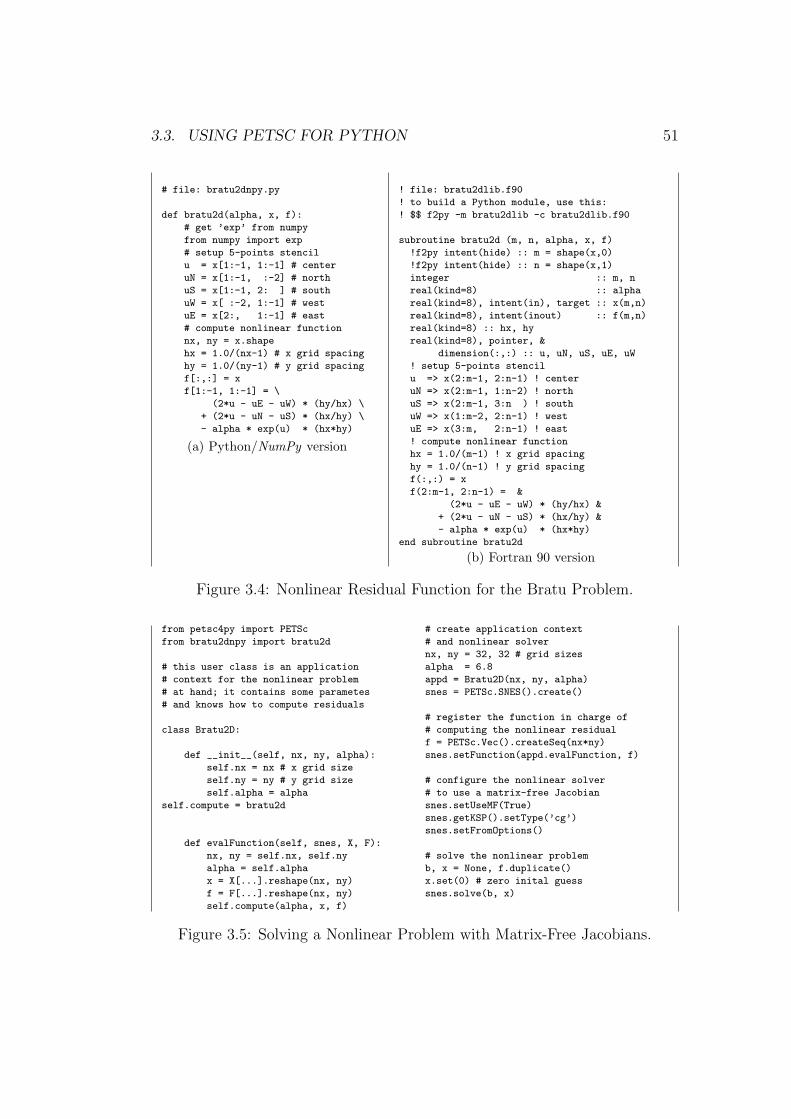
3.3. USING PETSC FOR PYTHON 51
# file: bratu2dnpy.py
def bratu2d(alpha, x, f):
# get ’exp’ from numpy
from numpy import exp
# setup 5-points stencil
u = x[1:-1, 1:-1] # center
uN = x[1:-1, :-2] # north
uS = x[1:-1, 2: ] # south
uW = x[ :-2, 1:-1] # west
uE = x[2:, 1:-1] # east
# compute nonlinear function
nx, ny = x.shape
hx = 1.0/(nx-1) # x grid spacing
hy = 1.0/(ny-1) # y grid spacing
f[:,:] = x
f[1:-1, 1:-1] = \
(2*u - uE - uW) * (hy/hx) \
+ (2*u - uN - uS) * (hx/hy) \
- alpha * exp(u) * (hx*hy)
(a) Python/NumPy version
! file: bratu2dlib.f90
! to build a Python module, use this:
! $$ f2py -m bratu2dlib -c bratu2dlib.f90
subroutine bratu2d (m, n, alpha, x, f)
!f2py intent(hide) :: m = shape(x,0)
!f2py intent(hide) :: n = shape(x,1)
integer :: m, n
real(kind=8) :: alpha
real(kind=8), intent(in), target :: x(m,n)
real(kind=8), intent(inout) :: f(m,n)
real(kind=8) :: hx, hy
real(kind=8), pointer, &
dimension(:,:) :: u, uN, uS, uE, uW
! setup 5-points stencil
u => x(2:m-1, 2:n-1) ! center
uN => x(2:m-1, 1:n-2) ! north
uS => x(2:m-1, 3:n ) ! south
uW => x(1:m-2, 2:n-1) ! west
uE => x(3:m, 2:n-1) ! east
! compute nonlinear function
hx = 1.0/(m-1) ! x grid spacing
hy = 1.0/(n-1) ! y grid spacing
f(:,:) = x
f(2:m-1, 2:n-1) = &
(2*u - uE - uW) * (hy/hx) &
+ (2*u - uN - uS) * (hx/hy) &
- alpha * exp(u) * (hx*hy)
end subroutine bratu2d
(b) Fortran 90 version
Figure 3.4: Nonlinear Residual Function for the Bratu Problem.
from petsc4py import PETSc
from bratu2dnpy import bratu2d
# this user class is an application
# context for the nonlinear problem
# at hand; it contains some parametes
# and knows how to compute residuals
class Bratu2D:
def __init__(self, nx, ny, alpha):
self.nx = nx # x grid size
self.ny = ny # y grid size
self.alpha = alpha
self.compute = bratu2d
def evalFunction(self, snes, X, F):
nx, ny = self.nx, self.ny
alpha = self.alpha
x = X[...].reshape(nx, ny)
f = F[...].reshape(nx, ny)
self.compute(alpha, x, f)
# create application context
# and nonlinear solver
nx, ny = 32, 32 # grid sizes
alpha = 6.8
appd = Bratu2D(nx, ny, alpha)
snes = PETSc.SNES().create()
# register the function in charge of
# computing the nonlinear residual
f = PETSc.Vec().createSeq(nx*ny)
snes.setFunction(appd.evalFunction, f)
# configure the nonlinear solver
# to use a matrix-free Jacobian
snes.setUseMF(True)
snes.getKSP().setType(’cg’)
snes.setFromOptions()
# solve the nonlinear problem
b, x = None, f.duplicate()
x.set(0) # zero inital guess
snes.solve(b, x)
Figure 3.5: Solving a Nonlinear Problem with Matrix-Free Jacobians.

52 CHAPTER 3. PETSC FOR PYTHON
3.4 Efficiency Tests
In the context of scientific computing, Python is commonly used as glue lan-
guage for interconnecting different pieces of codes written in compiled lan-
guages like C, C++ and Fortran. By using this approach, complex scientific
applications can take advantage of the best features of both worlds: the con-
venient, high-level programming environment of Python and the efficiency of
compiled languages for numerically intensive computations.
This section presents some efficiency tests targeted to measure the overhead
of accessing PETSc functionalities through PETSc for Python. The overhead
is determined by comparing the wall-clock running time of equivalent driving
codes implemented in Python and C. Both codes employ PETSc iterative linear
solvers and an auxiliary Fortran routine in charge of performing application-
specific computations. The actual application deals with the numerical solu-
tion of a model linear partial differential equation using Krylov-based iterative
linear solvers in combination with matrix-free techniques.
3.4.1 The Poisson Problem
Consider the following Poisson problem in three dimensions equipped with
homogeneous boundary conditions:
−∆φ = 1 on Ω,
φ = 0 at Γ;
where Ω is the unit box (0, 1)3 and Γ is the entire box boundary, ∆ is the
three-dimensional Laplace operator, and φ is a scalar field defined on Ω.
From the many discretization methods suitable for the above problem, finite
differences is the chosen one; this method can be easily and efficiency imple-
mented in Fortran 90 with a few lines of code. Thus, the spatial discretization
is performed with finite differences using the standard 7-points stencil on a
structured, regularly spaced grid. For the sake of simplicity, the discrete grid
is assumed to have the same number of nodes on each of its three directions.
For a given discrete grid having n+2 points in each direction, a system of lin-

3.4. EFFICIENCY TESTS 53
ear equations with n3 equations and n3 unknowns is obtained. The associated
discrete linear operator is symmetric and positive definite.
3.4.2 A Matrix-Free Approach for the Linear Problem
The system of linear equations arising from the spatial discretization can be
approximately solved by using Krylov-based iterative methods. Those methods
are suitable for employing matrix-free representations of linear operators. In
matrix-free techniques, the entries of the linear system matrix are not explicitly
stored. Instead, the linear operator is implicitly defined by its action on a given
input vector.
Figure 3.6 shows the complete implementation of a matrix-free linear op-
erator for the problem at hand. In figure 3.6b, the auxiliary Fortran code
implements a routine in charge of computing the action of the (negative) dis-
crete Laplacian. This implementation takes advantage of multi-dimensional
array processing; a careful look reveals that an auxiliary input array is being
employed in order to simplify the handling of boundary conditions. This rou-
tine is easily made available to Python by using F2Py. In figure 3.6a, a Python
class implements some selected methods of the generic interface for user-defined
linear operators. The mult() method receives the input and output vectors
and calls the previously discussed Fortran routine in order to actually compute
the action of the discrete Laplace operator. Other two additional methods are
also implemented: multTranspose() and getDiagonal().
Figure 3.7 shows how the previous codes are combined in order to actually
solve the linear system of equations. A shell PETSc matrix is created with
appropriate row and column sizes. This matrix is associated with an instance
of the user-defined matrix class previously implemented as shown in figure 3.6.
From the matrix object, appropriately sized vectors for storing the solution
and right hand side are obtained; all right hand side vector entries are set to
one. Next, a PETSc linear solver is created and configured to use conjugate
gradients with no preconditioner. Finally, the linear system of equations is
solved and the solution vector is scaled in order to account for the grid spacing.
For the sake of completeness, figures 3.8 and 3.9 show a complete C im-

54 CHAPTER 3. PETSC FOR PYTHON
# file: del2mat.py
from numpy import zeros
from del2lib import del2apply
class Del2Mat:
def __init__(self, n):
self.N = (n, n, n)
self.F = zeros([n+2]*3, order=’f’)
def mult(self, x, y):
"y <- A * x"
N, F = self.N, self.F
# get 3D arrays from vectos
xx = x[...].reshape(N, order=’f’)
yy = y[...].reshape(N, order=’f’)
# call Fortran subroutine
del2apply(F, xx, yy)
def multTranspose(self, x, y):
"y <- A’ * x"
self.mult(x, y)
def getDiagonal(self, D):
"D[i] <- A[i,i]"
D[...] = 6.0
(a) Python class defining a shell matrix
! file: del2lib.f90
! to build a Python module, use this:
! $$ f2py -m del2lib -c del2lib.f90
subroutine del2apply (n, F, x, y)
!f2py intent(hide) :: n=shape(F,0)-2
integer :: n
real(kind=8) :: F(0:n+1,0:n+1,0:n+1)
real(kind=8) :: x(n,n,n)
real(kind=8) :: y(n,n,n)
F(1:n,1:n,1:n) = x
y(:,:,:) = 6.0 * F(1:n,1:n,1:n) &
- F(0:n-1,1:n,1:n) &
- F(2:n+1,1:n,1:n) &
- F(1:n,0:n-1,1:n) &
- F(1:n,2:n+1,1:n) &
- F(1:n,1:n,0:n-1) &
- F(1:n,1:n,2:n+1)
end subroutine del2apply
(b) Finite differences in Fortran 90
Figure 3.6: Defining a Matrix-Free Operator for the Poisson Problem.
from petsc4py import PETSc
from del2mat import Del2Mat
# number of nodes in each direction
# excluding those at the boundary
n = 32
h = 1.0/(n+1) # grid spacing
# setup linear system matrix
A = PETSc.Mat().create()
A.setSizes([n**3, n**3])
A.setType(’shell’)
shell = Del2Mat(n) # shell context
A.setShellContext(shell)
# setup linear system vectors
x, b = A.getVecs()
x.set(0.0)
b.set(1.0)
# setup Krylov solver
ksp = PETSc.KSP().create()
pc = ksp.getPC()
ksp.setType(’cg’)
pc.setType(’none’)
ksp.setFromOptions()
# iteratively solve linear
# system of equations A*x=b
ksp.setOperators(A)
ksp.solve(b, x)
# scale solution vector to
# account for grid spacing
x.scale(h**2)
Figure 3.7: Solving a Matrix-Free Linear Problem with PETSc for Python.

3.4. EFFICIENCY TESTS 55
plementation equivalent to the Python one previously discussed and shown in
figures 3.6a and 3.7. This C code reuses the Fortran subroutine implementing
the finite difference scheme shown in figure 3.6b.
3.4.3 Some Selected Krylov-Based Iterative Methods
Conjugate gradient iterations are the natural choice for iteratively solving a
system of linear equations with symmetric and positive definite operators.
However, the solution of linear problem at hand can also be found with other
Krylov-based linear solvers tailored to more general problems. For the testing
purposes of this section, four different solvers readily implemented in PETSc
and available through PETSc for Python are employed.
The following list summarizes some aspects of the selected Krylov-based
iterative methods regarding to their applicability, storage requirements (work
vectors) for the unpreconditioned versions and involved computational ker-
nels (vector inner products, vector updates, and matrix-vector products). For
further details, see [42] and references therein.
• Conjugate Gradient Method (CG): this method is suitable for sym-
metric and positive definite linear problems. CG requires very few mem-
ory resources: it can be implemented with just two work vectors. At each
iteration, CG requires a small, fixed amount of computation (two inner
products and three vector updates) and only one matrix-vector product.
• Minimal Residual Method (MINRES ): this method is suitable for
symmetric indefinite linear problems. MINRES requires eight work vec-
tors and the computation of more vector primitives than CG . However,
MINRES can be employed in any symmetric problem, not just the pos-
itive definite ones. At each iteration, MINRES requires a fixed amount
computation and only one matrix-vector product.
• BiConjugate Gradient Stabilized (BiCGStab): this method is suit-
able for general linear problems. BiCGStab requires five additional work
vectors. At each iteration, BiCGStab requires a moderated and fixed
amount computation (four inner products and six vector updates) and
two matrix-vector products.

56 CHAPTER 3. PETSC FOR PYTHON
/* file: del2mat.h */
#ifndef DEL2MAT_H
#define DEL2MAT_H
#include <petsc.h>
#include <petscvec.h>
#include <petscmat.h>
/* external Fortran subroutine */
#define Del2Apply del2apply_
extern void Del2Apply(int*,double*,double*,double*);
/* user data structure and routines
* defining the matrix-free operator */
typedef struct
PetscInt N;
PetscScalar *F;
Del2Mat;
#undef __FUNCT__
#define __FUNCT__ "Del2Mat_mult"
/* y <- A * x */
PetscErrorCode Del2Mat_mult(Mat A, Vec x, Vec y)
Del2Mat *ctx;
PetscScalar *xx,*yy;
PetscErrorCode ierr;
PetscFunctionBegin;
ierr = MatShellGetContext(A,(void**)&ctx);CHKERRQ(ierr);
/* get raw vector arrays */
ierr = VecGetArray(x,&xx);CHKERRQ(ierr);
ierr = VecGetArray(y,&yy);CHKERRQ(ierr);
/* call external Fortran subroutine */
Del2Apply(&ctx->N,ctx->F,xx,yy);
/* restore raw vector arrays */
ierr = VecRestoreArray(x,&xx);CHKERRQ(ierr);
ierr = VecRestoreArray(y,&yy);CHKERRQ(ierr);
PetscFunctionReturn(0);
#undef __FUNCT__
#define __FUNCT__ "Del2Mat_diag"
/*D_i <- A_ii */
PetscErrorCode Del2Mat_diag(Mat A, Vec D)
PetscErrorCode ierr;
PetscFunctionBegin;
ierr = VecSet(D,6.0);CHKERRQ(ierr);
PetscFunctionReturn(0);
#endif
Figure 3.8: Defining a Matrix-Free Operator, C implementation.

3.4. EFFICIENCY TESTS 57
#include "del2mat.h"
#include <petscksp.h>
#define DEL2MAT_MULT ((void(*)(void))Del2Mat_mult)
#define DEL2MAT_DIAG ((void(*)(void))Del2Mat_diag)
int main(int argc,char **argv)
PetscInt n;
PetscScalar h;
Del2Mat shell;
Mat A;
Vec x,b;
KSP ksp;
PC pc;
/* PETSc initialization */
PetscInitialize(&argc, &argv, PETSC_NULL, PETSC_NULL);
/* number of nodes in each direction
* excluding those at the boundary */
n = 32;
h = 1.0/(n+1); /* grid spacing */
/* setup linear system (shell) matrix */
MatCreate(PETSC_COMM_SELF, &A);
MatSetSizes(A, n*n*n, n*n*n, n*n*n, n*n*n);
MatSetType(A, MATSHELL);
shell.N = n;
PetscMalloc((n+2)*(n+2)*(n+2)*sizeof(PetscScalar),&shell.F);
PetscMemzero(shell.F, (n+2)*(n+2)*(n+2)*sizeof(PetscScalar));
MatShellSetContext(A, (void**)&shell);
MatShellSetOperation(A, MATOP_MULT, DEL2MAT_MULT);
MatShellSetOperation(A, MATOP_MULT_TRANSPOSE, DEL2MAT_MULT);
MatShellSetOperation(A, MATOP_GET_DIAGONAL, DEL2MAT_DIAG);
/* setup linear system vectors */
MatGetVecs(A, &x, &b);
VecSet(x, 0);
VecSet(b, 1);
/* setup Krylov linear solver */
KSPCreate(PETSC_COMM_SELF, &ksp);
KSPGetPC(ksp, &pc);
KSPSetType(ksp, KSPCG); /* use conjugate gradients */
PCSetType(pc, PCNONE); /* with no preconditioning */
KSPSetFromOptions(ksp);
/* iteratively solve linear system of equations A*x=b */
KSPSetOperators(ksp,A,A,SAME_NONZERO_PATTERN);
KSPSolve(ksp, b, x);
/* scale solution vector to account for grid spacing */
VecScale(x, h*h);
/* free memory and destroy objects */
PetscFree(shell.F);
MatDestroy(A);
VecDestroy(x);
VecDestroy(b);
KSPDestroy(ksp);
/* finalize PETSc */
PetscFinalize();
return 0;
Figure 3.9: Solving a Matrix-Free Linear Problem, C implementation.

58 CHAPTER 3. PETSC FOR PYTHON
• Generalized Minimal Residual Method (GMRES ): this method is
suitable for general linear problems. While iterating, GMRES construct
a orthonormal basis for the Krylov subspace by inserting new vectors ob-
tained through some orthogonalization procedure. Therefore, GMRES
requires an additional work vector and an increasing amount of compu-
tation (i+1 inner products and i+1 vector updates, being i the iteration
number) of at each new iteration. Practical implementations limit the
size of the Krylov basis by restarting the iterative process; this variant
is usually denoted as GMRES (m), where m is the maximum size of the
Krylov basis. At each iteration, GMRES requires only one matrix-vector
product.
3.4.4 Measuring Overhead
Tests were run sequentially on one computing node of the cluster Aquiles [34].
The software and hardware components were the ones previously described in
section 2.5. Additionally, PETSc 2.3.3-p6 was employed.
Results are shown in figures 3.11, 3.13, 3.15, and 3.17. The overhead is
determined as (TPy/TC) − 1, where TPy and TC are the measured wall clock
times spent by the Python implementation (see figures 3.6 and 3.7) and the
C implementation (see figures 3.8 and 3.9) respectively in solving the problem
at hand for different levels of discretization. Additionally, figures 3.11, 3.13,
3.15, and 3.17 show the convergence histories of the methods for some selected
number of unknowns.
The general trend is the expected one: as the number of unknowns grows,
the overhead of PETSc for Python diminishes. Figure 3.10 shows together the
results for the CG and GMRES cases. CG method exhibits greater overhead
for a given problem size. Indeed, of the four methods CG and BiCGStab are the
ones with the lowest amount of vector-vector operations versus matrix-vector
operations. Therefore, the overhead of applying the matrix-vector product
from the Python layers is more significant. On the other way, GMRES exhibits
the lowest overhead, as it is the method requiring the highest amount of inner
vector-vector operations.

3.4. EFFICIENCY TESTS 59
301
351
302
352
303
353
304
354
305
355
Unknowns [#]
0
5
01
51
02
52
03
53
04
54
Overh
ead [
%]
CGGMRES(30)
Figure 3.10: Comparing Overhead Results for CG and GMRES (30).

60 CHAPTER 3. PETSC FOR PYTHON
301
302
303
304
305
306
307
Unknowns [#]
0
5
01
51
02
52
03
53
04
54
Overh
ead [
%]
CG
Figure 3.11: PETSc for Python Overhead using CG .
0 20 40 60 80 100 120Iterations
10-6
10-5
10-4
10-3
10-2
10-1
100
101
Resid
ual N
orm
CG
323
384
346
Figure 3.12: Residual History using CG .

3.4. EFFICIENCY TESTS 61
301
302
303
304
305
306
307
Unknowns [#]
0
5
01
51
02
52
03
53
Overh
ead [
%]
MINRES
Figure 3.13: PETSc for Python Overhead using MINRES .
0 20 40 60 80 100 120Iterations
10-6
10-5
10-4
10-3
10-2
10-1
100
Resid
ual N
orm
MINRES
323
384
346
Figure 3.14: Residual History using MINRES .
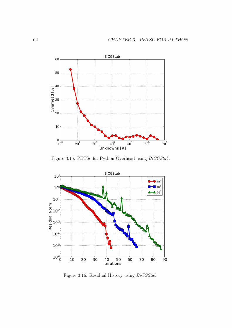
62 CHAPTER 3. PETSC FOR PYTHON
301
302
303
304
305
306
307
Unknowns [#]
0
01
02
03
04
05
06
Overh
ead [
%]
BiCGStab
Figure 3.15: PETSc for Python Overhead using BiCGStab.
0 10 20 30 40 50 60 70 80 90Iterations
10-6
10-5
10-4
10-3
10-2
10-1
100
101
Resid
ual N
orm
BiCGStab
323
384
346
Figure 3.16: Residual History using BiCGStab.

3.4. EFFICIENCY TESTS 63
351
302
352
303
353
304
354
305
Unknowns [#]
0
5
01
51
02
52
Overh
ead [
%]
GMRES(30)
Figure 3.17: PETSc for Python Overhead using GMRES (30).
0 50 100 150 200 250 300 350 400Iterations
10-6
10-5
10-4
10-3
10-2
10-1
100
Resid
ual N
orm
GMRES(30)
323
384
346
Figure 3.18: Residual History using GMRES (30).


Chapter 4
Electrokinetic Flow in
Microfluidic Chips
This chapter discusses the theoretical modeling and numerical simulations of
electrokinetic and transport phenomena in microfluidic chips, considering ef-
fects in three dimensions and whole geometries. The modeling grounds on
conservation equations of mass, momentum and electric charge in the frame-
work of continuum mechanics. An example of interest in electrophoresis chips
is considered as study case.
All numerical simulations presented in this chapter are performed with
PETSc-FEM [12, 43] within the Python programming environment described
in previous chapters. PETSc-FEM is a parallel multi-physics code primar-
ily targeted to 2D and 3D finite elements computations on general unstruc-
tured grids. PETSc-FEM is based on MPI and PETSc, it is being devel-
oped since 1999 at the International Center for Numerical Methods in Engi-
neering (CIMEC), Argentina. PETSc-FEM provides a core library in charge
of managing parallel data distribution and assembly of residual vectors and
Jacobian matrices, as well as facilities for general tensor algebra computa-
tions at the level of problem-specific finite element routines. Additionally,
PETSc-FEM provides a suite of specialized application programs built on
top of the core library but targeted to a variety or problems (e.g., compress-
ible/incompressible Navier–Stokes and compressible Euler equations, general
65

66 CHAPTER 4. ELECTROKINETIC FLOW IN MICROFLUIDIC CHIPS
advective-diffusive systems, weak/strong fluid-structure interaction). In par-
ticular, fluid flow computations presented in this chapter are carried out within
the Navier–Stokes module available in PETSc-FEM. This module provides the
required capabilities for simulating incompressible fluid flow through a mono-
lithic SUPG/PSPG [44, 45] stabilized formulation for linear finite elements.
4.1 Background
Microfluidic chips or micro Total Analysis Systems (µ–TAS) perform the func-
tions of large analytical devices in small units [46]. They are used in a variety
of chemical, biological and medical applications. The benefits of µ–TAS are
a reduction of consumption of samples and reagents, shorter analysis times,
greater sensitivity, portability and disposability. There has been a huge in-
terest in these devices in the past decade that led to a commercial range of
products by Caliper, Agilent, Shimadzu and Hitachi [47].
Most microfluidic systems have been successfully fabricated in glass or ox-
idized silicon [48]. Microscopic channels are defined in these substrates using
photolithography and micromachining, whose materials and fabrication meth-
ods were adopted from the microelectronics industry. However, for the pur-
poses of rapid prototyping and testing of new concepts, the fabrication pro-
cesses are slow and expensive.
Figure 4.1: Microfluidic Chips.

4.1. BACKGROUND 67
Numerical simulations of on-chip processes can serve to reduce the time
from concept to chip [49]. Some of the first numerical simulations of flow and
species transport for microfluidic chips were based on electrokinetic focusing
and sample dispensing techniques. Patankar and Hu [50] employed an algo-
rithm based on a finite differences discretization of the governing equations on
a structured grid to simulate those techniques. Bianchi et al. [51] performed
2D finite element simulations artificially increasing the electric double layer
thickness. 3D finite volume simulations have been also performed [52, 53].
Erickson [54] investigated electroosmotic flow in heterogeneous surfaces with
a 3D finite element model on a simultaneous solution to the Nernst–Planck,
Poisson and Navier–Stokes equations.
Microfluidic chips developed for capillary electrophoresis integrates a net-
work of microchannels, reservoirs and electrodes, as the transport of fluids is
driven by the action of external electric fields. Most of studies reported in the
literature focus on microchannels or particular regions of the network, disre-
garding the influence of reservoirs and electrodes. Nevertheless, these elements
may significantly alter the electroosmotic velocity profile, and hence sample
dispersion. For instance, the connections between reservoirs and microchan-
nels involve sudden contractions/expansions that induce pressure gradients;
the electric field at the inlet/outlet of microchannels depends on the position
of the electrode in the reservoir. Achieving numerical simulations of the whole
microfluidic system is crucial to assist the design, control and optimization of
analytical manipulations.
The most interesting aspect of computational simulation of microfluidic
chips is the multiphysics nature which combines fluidics, transport, thermal,
mechanics, electronics and optics with chemical, biological thermodynamics
and reaction kinetics. Additionally, studying theses effects is a challenging
problem from the numerical point of view. They comprise geometrical scales
that span six orders of magnitude: from the millimetric size of reservoirs,
passing by the micrometric width of channels, to the nanomentric thickness of
the electric double layer at interfaces.

68 CHAPTER 4. ELECTROKINETIC FLOW IN MICROFLUIDIC CHIPS
4.2 Theoretical Modeling
The foundations of electrokinetic flow are well documented in the litera-
ture [55, 56]. The case of integrated microchannel networks filled with aqueous
electrolyte solutions is considered here. The electrostatic charges present at
the solid-liquid interface involve an electric potential that decreases steeply in
the liquid due to the screening produced by dissolved counterions and other
electrolyte ions, which constitute the electric double layer.
4.2.1 Governing Equations
Electrokinetic effects arise when there is a movement of the liquid and as-
sociated ions in relation to the solid. In the framework of continuum fluid
mechanics, fluid velocity u, pressure p, and electric E fields are governed by
the following set of coupled equations [57, 58, 59],
−∇ ·u = 0, (4.1)
ρ(∂u
∂t+ u ·∇u) = ∇ ·σ + ρg + ρeE, (4.2)
ε∇ ·E = ρe . (4.3)
Equation 4.1 expresses the conservation of mass for incompressible flu-
ids. Equation 4.2 (Navier–Stokes equation) expresses the conservation of
momentum for Newtonian fluids of density ρ, viscosity µ, and stress tensor
σ = −pI + µ(∇u + ∇uT ), subjected to gravitational field of acceleration g
and electric field intensity E. The last term on the right hand side of equa-
tion 4.2 represents the contribution of electrical forces to the momentum bal-
ance, where ρe = F∑
k zkck is the electric charge density of the electrolyte
solution, obtained as the summation over all type-k ions, with valence zk and
molar concentration ck, and F is the Faraday constant.
Equation 4.3 (Poisson equation) establishes the relation between electric
potential and charge distributions in the fluid of permittivity ε. Here it is rel-
evant to mention that the ion distributions ck (to be included in equations 4.2
and 4.3 through ρe must be derived from Nernst-Planck equation, which ac-

4.2. THEORETICAL MODELING 69
counts for the flux of type-k ions due to electrical forces, fluid convection and
Brownian diffusion [56]. This coupling can be avoided by introducing a suitable
simplification (see section 4.2.2).
One of the most used manipulations in microfluidic chips is electrophoretic
separation of charged molecules. Thus the present work also considers the
following transport equation
∂cj
∂t+ u ·∇cj = Dj∇2cj −∇ · (νjzjcjFE) , (4.4)
which governs the molar concentration cj of type-j species in the electrolyte
solution. In equation 4.4, Dj is the diffusion coefficient, νj is the mobility, and
F is the Faraday constant. Therefore, once velocity u and electric field E are
obtained from equations 4.1-4.3, the molar concentration profile cj of different
j species is derived from equation 4.4.
4.2.2 Electrokinetic Phenomena
Generally, most substances will acquire a surface electric charge when brought
into contact with an aqueous (polar) medium. Some of the charging mecha-
nisms include ionization, ion adsorption, and ion dissolution. The effect of any
charged surface in an electrolyte solution will be to influence the distribution of
nearby ions in the solution. Ions of opposite charge to that the surface (coun-
terions) are attracted towards the surface while ions of like charge (coions) are
repelled from the surface. This attraction and repulsion, when combined with
the mixing tendency resulting from the random thermal motions of the ions,
leads to the formation of an electric double layer (see figure 4.3 at page 72).
The electric double layer is a region close to the charged surface in which
there is an excess of counterions over coions to neutralize the surface charge,
and these ions are spatially distributed in a “diffuse” manner. Evidently there
is no charge neutrality withing the double layer because the number of counte-
rions will be large compared with the number of coions. The generated electric
potentials are on the order of 50 mV. When moving away from the surface,
the potential progressively decreases, and then vanishes in the liquid phase.

70 CHAPTER 4. ELECTROKINETIC FLOW IN MICROFLUIDIC CHIPS
Electric Double Layer Theory
Consider a simple fully dissociated symmetrical salt in solution for which the
number of positive and negative ions are equal, so
z+ = −z− = z . (4.5)
When this electrolyte solution is brought into contact with a solid such that the
surface of contact becomes positively charged, the concentrations of positive
and negative ions has the following Boltzmann distribution
c± = c0 exp
(∓zF
RTφ
); (4.6)
where φ is the electric potential, c0 is the bulk salt concentration, R is the ideal
gas constant and T is the absolute temperature. Clearly, the ion concentrations
far from the surface c± → c0 as φ → 0.
Under the above assumptions, the electric charge density is
ρe = F∑
k
zkck
= F
[+zc0 exp
(−zF
RTφ
)− zc0 exp
(+zF
RTφ
)]= 2zc0F sinh
(− zF
RTφ
);
(4.7)
and the electric field E is related to the electric potential φ through
E = −∇φ . (4.8)
Equations 4.7 and 4.8 can be inserted in the Poisson equation 4.3 to finally
obtain
−∇2φ =2zc0F
εsinh
(− zF
RTφ
). (4.9)
The electric potential φ obtained through solving the Poisson–Boltzmann
equation 4.9 can then be employed for determining the electric field E (equa-
tion 4.8) and the electric charge density ρe (equation 4.7). The electrical forces

4.2. THEORETICAL MODELING 71
can then be computed and entered in the momentum equation 4.2.
Electric Double Layer Thickness
The electric double layer thickness may be approximately quantified through
the Debye length [55, 56],
λD =
√εRT
2z2cF 2; (4.10)
were c is taken to be the average molar negative ion (counterion) concentration.
0 Dλ
Distance
0cC
oncentration
counterions
coions
bulk
0 Dλ
Distance
wφ
Potential
Figure 4.2: The Diffuse Double Layer and the Debye Length.
The Debye length represents the position where the electrical potential
energy is approximately equal to the thermal energy of the counterions. It is
obtained by neglecting the presence of coions and solving a simplified Poisson
problem in the one-dimensional picture of figure 4.2.
For the ionic concentrations normally used in practice, λD is on the order
of 10 nm. Away from the interface, at distances beyond λD, the bulk of the
fluid is electrically neutral.

72 CHAPTER 4. ELECTROKINETIC FLOW IN MICROFLUIDIC CHIPS
Electroosmotic Flow and Slip Velocity Approximation
Electroosmotic flow in microchannels grounds on the existence excess of ions
in the fluid near solid walls. When an external electric field is applied in the
axial direction of a channel, the electrical forces acting on excess ions drag the
surrounding liquid and then electroosmotic flow develops.
Figure 4.3: Electroosmotic Flow.
For thin electric double layer in relation to the channel width h, electroos-
motic phenomena is confined to regions close to channel walls. Under these
conditions, the electroosmotically driven flow can be regarded as the result
of an electrically-induced slip velocity ; its magnitude can be approximated
by [55, 56]
uEO =εζ
µE ; (4.11)
where ζ is the electrokinetic potential.
Further, uEO can be used as a boundary value at the channel walls. This
possibility greatly simplifies calculations since ion distributions are decoupled
from Navier–Stokes and Poisson equations. In fact, if ion concentrations are
assumed to be uniform (except in the close vicinity of the charged interface),
and hence throughout the flow domain, the right hand side of equation 4.3
vanishes, as well as the last term of equation 4.2.
4.3. NUMERICAL SIMULATIONS 73
The slip velocity approximation is valid for small values of λD/h, which
is usually the case in micro-scale channels at moderate ionic concentrations
(≈ 10−3 M). Nevertheless, at very low ionic concentrations (≈ 10−6 M), or in
case of nanoscale channels, λD/h approaches one, indicating that the electric
double layer from opposing surfaces overlap. In that case, approximation 4.11
does not apply and the full problem must be solved.
4.3 Numerical Simulations
Previous works related to numerical simulation of electroosmotic flow and elec-
trophoresis have restricted the problem domain to the microchannels by sup-
posing appropriate conditions for the electric potential, velocity field, and con-
centrations at inlet and outlet regions. In this section, results from numerical
simulations performed on a whole microfluidic system domain are presented.
The influence of components like electrodes and reservoirs is investigated in
order to estimate their actual significance in electroosmotic flow phenomena
in general and electrophoretic separation processes in particular.
The simulations domain is a a cross-shaped microchannel network with
vertical wire electrodes at reservoirs. The channel network is fabricated on a
glass microscope slide with dimensions 75 mm×25 mm×1 mm. The channel
sections are trapezoidal, with shape and dimensions as shown in figure 4.4.
Electrophoretic injection and separation processes are simulated in order
to determine potassium and sodium ion concentrations. During the injection
stage, the potentials at electrodes is selected in such a way that the intersection
region is filled with a precise sample volume to be analyzed. In the separation
stage, the potentials at electrodes is appropriately selected in order to achieve
different relative velocities for each specie, avoiding leakages at the injection
channels. The values of the relevant physical properties and constants are
summarized in table 4.1.
The complete simulations requires the solution of three subsidiary prob-
lems involving charge, mass, momentum and species conservation equations
described in section 4.1.
The electric fields are obtained through solving Poisson equation 4.3 (with
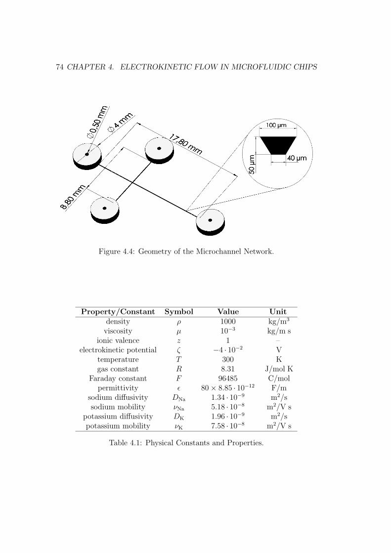
74 CHAPTER 4. ELECTROKINETIC FLOW IN MICROFLUIDIC CHIPS
Figure 4.4: Geometry of the Microchannel Network.
Property/Constant Symbol Value Unitdensity ρ 1000 kg/m3
viscosity µ 10−3 kg/m sionic valence z 1 –
electrokinetic potential ζ −4 · 10−2 Vtemperature T 300 Kgas constant R 8.31 J/mol K
Faraday constant F 96485 C/molpermittivity ε 80× 8.85 · 10−12 F/m
sodium diffusivity DNa 1.34 · 10−9 m2/ssodium mobility νNa 5.18 · 10−8 m2/V s
potassium diffusivity DK 1.96 · 10−9 m2/spotassium mobility νK 7.58 · 10−8 m2/V s
Table 4.1: Physical Constants and Properties.

4.3. NUMERICAL SIMULATIONS 75
ρe = 0) for the potential and employing Dirichlet boundary conditions at
electrodes and homogeneous Neumann boundary conditions at channels and
reservoirs walls.
Fluid velocity is obtained by solving mass conservation equation 4.1 and
Navier–Stokes equation 4.1 is stationary mode and employing as boundary
condition the slip velocity approximation (equation 4.11) at the channels walls.
Finally, transport equation 4.4 is solved for the concentrations of Na+ and
Ka+ ions by employing the electric field and fluid velocity previously obtained.
This problem is transient; initial concentrations (at t = 0 s) are set to zero
everywhere except at one of the reservoirs as shown in figure 4.5.
Figure 4.5: Initial Na+ and Ka+ Ions Concentrations (mol/m3)
Figure 4.6 shows the applied potentials and the final (at t = 10 s) concen-
tration distributions of Na+ and Ka+ ions during the injection stage. Figure 4.7
shows the applied potentials and concentration distributions of Na+ and Ka+
ions at some moment (t = 15 s) during the separation stage.

76 CHAPTER 4. ELECTROKINETIC FLOW IN MICROFLUIDIC CHIPS
(a) applied potentials (V)
(b) ions concentrations (mol/m3)
Figure 4.6: Injection Stage.

4.3. NUMERICAL SIMULATIONS 77
(a) applied potentials (V)
(b) ions concentrations (mol/m3)
Figure 4.7: Separation Stage.
78 CHAPTER 4. ELECTROKINETIC FLOW IN MICROFLUIDIC CHIPS
4.4 Classical Domain Decomposition Methods
Domain Decomposition Methods (DDM) [60] are divide and conquer techniques
for solving boundary value problem by splitting it into smaller boundary value
problems on subdomains and iterating to coordinate the solution between the
subdomains. The problems on the subdomains are independent, which makes
domain decomposition methods suitable for parallel computing on distributed
memory architectures. Domain decomposition methods are typically used as
preconditioners for Krylov space iterative methods, such as the Conjugate
Gradient (CG) method or Generalized Minimal Residual (GMRES) methods.
In non-overlapping methods (also called iterative substructuring methods),
the subdomains overlap only on their interface. In primal methods, such as
Balancing Domain Decomposition (BDD) and the enhaced version BDDC [61],
the continuity of the solution across subdomain interface is enforced by repre-
senting the value of the solution on all neighboring subdomains by the same
unknown. In dual methods, such as Finite Elements Tearing and Intercon-
necting (FETI), the continuity of the solution across the subdomain interface
is enforced by Lagrange multipliers. An enhaced, symplified and better per-
forming version of FETI, known as FETI-DP [62], is hybrid between a dual
and a primal method; its performance is essentially the same as the BDDC
method. BDD and FETI mathods were primarily developed for solving of
elliptic boundary value problems.
In overlapping domain decomposition methods, the subdomains overlap by
more than the interface. Overlapping domain decomposition methods include
the classical Schwarz alternating procedure and the Additive Schwarz Method
(ASM) [63]. Schwarz methods can be easily applied to a variety of prob-
lems [64, 65] and can be implemented in a fully-algebraic manner (i.e. without
knowledge of the underlying discrete grids).
This sections explores the applicability of additive Schwarz methods to a
model problem of interest in nanoscale fluid dynamics applications.

4.4. CLASSICAL DOMAIN DECOMPOSITION METHODS 79
4.4.1 A Model Problem
Consider an aqueous solution of a simple fully dissociated symmetrical salt
which flows on a channel driven by the action of electrical forces originated
from external electric fields. The values of the relevant physical properties and
constants are summarized in the following table
Property/Constant Symbol Value Unit
density ρ 1000 kg/m3
viscosity µ 10−3 kg/m s
ionic valence z 1 –
bulk concentration c0 10−2 mol/m3
electrokinetic potential ζ 2 · 10−2 V
temperature T 300 K
gas constant R 8.31 J/mol K
Faraday constant F 96485 C/mol
absolute permittivity ε 80× 8.85 · 10−12 F/m
The channel has an L-shaped geometry with an horizontal and vertical
lengths of 3 µm and a cross-section of 0.4 µm × 1 µm. As the electric double
layer thickness (estimated through the Debye length, equation 4.10) is around
0.1 µm, the slip velocity approximation (equation 4.11) cannot be employed.
A Laplace potential is computed by solving equation 4.3 with ρe = 0,
Dirichlet boundary conditions of 0.5 V at the inlet and 0 V at the outlet, and
homogeneous Neumann boundary conditions at the channel walls. A Poisson–
Boltzmann potential is computed by solving the nonlinear equation 4.9 with
Dirichlet boundary conditions of 20 mV (the electrokinetic potential) at the
channel walls and homogeneous Neumann boundary conditions at the channel
inlet and outlet. The solution for Poisson–Boltzmann potential is shown in
figure 4.8b. The Laplace and Poisson–Boltzmann potentials are added-up in
order to determine a total potential. Isolines of the total potential are shown
in 4.8c.
Finally, Navier–Stokes equations are solved by entering the electrical forces
as shown in equation 4.2. Electrical forces are determined from the total poten-
tial and Poisson–Boltzmann potential through equations 4.7 and 4.8. Non-slip
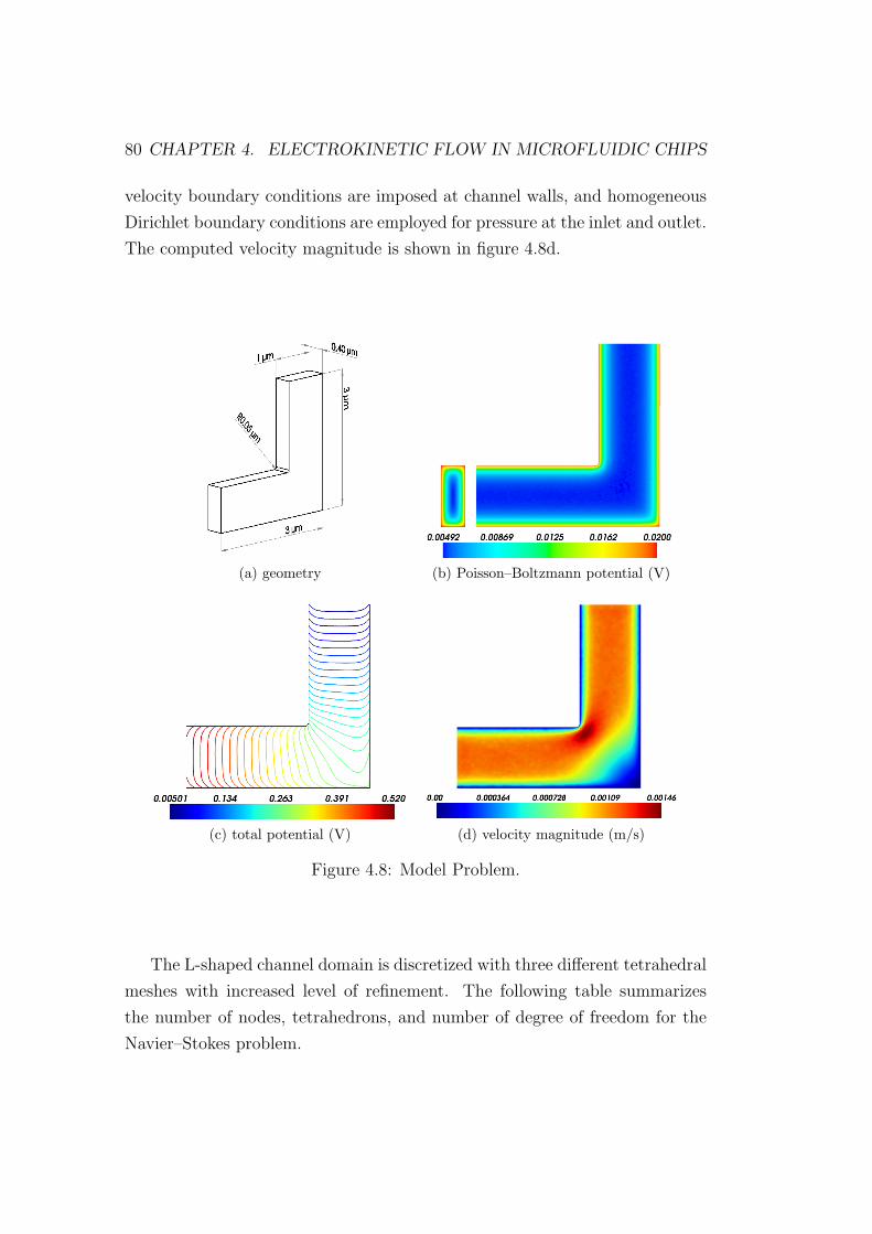
80 CHAPTER 4. ELECTROKINETIC FLOW IN MICROFLUIDIC CHIPS
velocity boundary conditions are imposed at channel walls, and homogeneous
Dirichlet boundary conditions are employed for pressure at the inlet and outlet.
The computed velocity magnitude is shown in figure 4.8d.
(a) geometry (b) Poisson–Boltzmann potential (V)
(c) total potential (V) (d) velocity magnitude (m/s)
Figure 4.8: Model Problem.
The L-shaped channel domain is discretized with three different tetrahedral
meshes with increased level of refinement. The following table summarizes
the number of nodes, tetrahedrons, and number of degree of freedom for the
Navier–Stokes problem.
4.4. CLASSICAL DOMAIN DECOMPOSITION METHODS 81
Mesh Nodes Elements DOF’s
#1 120,574 705,396 411,769
#2 235,011 1,406,195 828,746
#3 460,059 2,801,104 1,664,613
4.4.2 Additive Schwarz Preconditioning
The original alternating procedure described by Schwarz [66] in 1870 is an
iterative method to find the solution of a partial differential equations on a
domain which is the union of two overlapping subdomains, by solving the
equation on each of the two subdomains in turn, taking always the latest
values of the approximate solution as the boundary conditions.
The procedure described above is called the multiplicative Schwarz proce-
dure. In matrix terms, this is very reminiscent of a block Gauß–Seidel iteration.
The multiplicative Schwarz procedure is not fully parallel at the highest level:
some processors have to wait others in order to perform the local work. The
analogue of the block Jacobi procedure is known as the additive Schwarz pro-
cedure. The additive procedure is fully parallel; however, the convergence rate
is usually slower.
The application of the additive Schwarz procedure as a preconditioning
method for the solution of systems of linear equations can be summarized as
follows:
1. The support mesh/grid is decomposed into Ns (possibly overlapping)
subdomains Ωi, i = 1, . . . , Ns.
2. Each subdomain Ωi is associated to a local space Vi with the help of
a restriction operator Ri. The restriction operator Ri extract from the
global vector the unknowns associated with Ωi, while the extension op-
erators RTi extends by zeros unknowns from Ωi to the global vector. The
preconditioner operator can then be easily written in matrix terms as
P−1 =Ns∑i=1
RTi A−1
i Ri; (4.12)

82 CHAPTER 4. ELECTROKINETIC FLOW IN MICROFLUIDIC CHIPS
where Ai = RTi ARi are the local matrices associated with the subdo-
mains Ωi; they are related to the global matrix A through the restriction
operators Ri. In the special case of zero overlap, the matrices Ai have
entries from contributions originated in the subdomain Ωi; if the overlap
is greater than zero, the matrices Ai have additional entries contributed
by neighboring subdomains.
3. Any Krylov-based iterative method can then be employed for solving the
(left) preconditioned linear system P−1Ax = P−1b.
Many factors impact the performance of additive Schwarz preconditioning
in the context of parallel iterative methods for the solution of systems of linear
equations. The main ones are summarized in the following list.
• Additive Schwarz methods are normally implemented in such a way that
the number of subdomains Ns and the restriction operators Ri are in-
herited from the previous partitioning of the underlying discrete grid or
mesh. The local problems (involving matrix Ai in equation 4.12) are usu-
ally solved by variants of incomplete factorization methods (e.g. ILU(0)).
For well-conditioned problems, incomplete factorization methods are the
faster alternative regarding to overall wall-clock computing time.
• Iterative methods frequently stagnate when then global problem is ill-
conditioned and the local problems are treated with incomplete factor-
izations. In such cases, the local problems have to be solved either with
and inner iterative method or a full direct method (i.e. LU factoriza-
tion). In either case, as the size of the local subdomain increases, also do
the time required for obtaining the local solution. This is specially true
when the local solver is based on a LU factorization. In order to employ
a direct method and maintaining the size of local problems manageable,
local subdomains can be further partitioned at each processor in sub-
subdomains. This strategy degrades convergence, but can improve the
overall solution time.
• As the overlap increases, convergence rate improves; but computing,
communication and memory requirements increase. Ghost vector val-

4.4. CLASSICAL DOMAIN DECOMPOSITION METHODS 83
ues have to be gathered from and scattered to neighboring processors at
each iteration; matrix values have to be gathered from neighboring pro-
cessors in a setup phase, and the local problems to solve are larger (in
the setup-phase factorization as well as in the backward/forward solves
at each iteration). Then, as overlap increases, actual improvements in
the total wall-clock time for obtaining the final solution will depend upon
the balance between better convergence rates versus the extra costs.
• Finally, for global problems of medium to large scale, as the number
of processors assigned to its solution increases, the parallel efficiency
decreases. Actually, this behavior is shared for any non-embarrassingly
parallel algorithm. As a rule of thumb, each processor have to be in
charge of 50,000 to 100,000 unknowns (depending on computing and
network hardware) to achieve parallel speedup.
The rest of this subsection explores the issues commented previously by
applying the additive Schwarz preconditioner to the model problem on the
three discretizations described in subsection 4.4.1.
Although the problem at hand is essentially linear, it is solved as a full
nonlinear one employing two iteration of a standard Newton method. In all
the test cases, the final (outer, nonlinear) residual norm is reduced by a factor
of around 10−6.
The linear systems at each nonlinear step are solved with GMRES(250)
(i.e. GMRES restarted at 250 iterations) by defining a fixed relative tolerance
of 10−4 for the reduction of the initial (inner, linear) residual norm.
The additive Schwarz method is employed as a left-preconditioner within
GMRES iterations. Being the global linear systems of saddle-point nature,
they are ill-conditioned. Incomplete factorizations methods cannot be prac-
tically employed for the local problems, as this leads to GMRES stagnation.
Thus, the local problems are solved by employing full direct methods and ag-
gressive subdomain sub-partitioning at each processor. The sub-partitioning
is performed on the adjacency graph obtained from the local, diagonal part of
the global sparse matrix with the help of METIS [67] library.
84 CHAPTER 4. ELECTROKINETIC FLOW IN MICROFLUIDIC CHIPS
In all test cases discussed below, wall-clock time measurements do not ac-
count for the time required for evaluating and assembling residual vectors and
Jacobian matrices, but only for the time spent in solving the linear systems.
Parallel efficiency is computed by taking as reference the timings of the runs
performed on the smaller number of processes, i.e. Ep = (PminTPmin)/(pTp),
where p = Pmin, . . . , Pmax is the set of number of processes employed and Tp
is the wall-clock time measurement with p processes.
Figures 4.9 to 4.11 shows wall-clock time measurements and parallel effi-
ciency for the additive Schwarz preconditioner with overlap zero. The model
problem is solved on the meshes #1, #2, and #3 employing 20, 30, 40, and
50 processors. The subdomain sizes range from 1000 to 4000 unknowns. For
meshes #1 and #2, a subdomain size of around 1000 unknowns seems to be
optimal, while for mesh #3, the optimal subdomain size is around 2500 un-
knowns. Clearly, depending on the problem size, as the number of processors
increase beyond some limit the required wall-clock time for obtaining the so-
lution do not decrease but stagnates.
Remarkably, figure 4.10 shows that for the case of mesh #2, the solution
times are almost the same on 40 and 50 processors. Similarly, figure 4.11 shows
that for the case of mesh #3, the solution times are almost the same on 30,
40, and 50 processors. Figure 4.12 shows wall-clock time measurements and
parallel efficiency for the case of mesh #3 only on 16, 24, and 32 processors
and a broader range of subdomain sizes.
Finally, figure 4.13 shows wall-clock time measurements for the additive
Schwarz preconditioner with overlap zero and one. Clearly, increasing the
overlap also increases the solution time.

4.4. CLASSICAL DOMAIN DECOMPOSITION METHODS 85
500 1000 1500 2000 2500 3000 3500 4000Subdomain Size [unknowns]
0
5
10
15
20
25
30
Wall-C
lock T
ime [
seconds]
ASM(0) - Mesh 1
20 Processors30 Processors40 Processors50 Processors
500 1000 1500 2000 2500 3000 3500 4000Subdomain Size [unknowns]
0.0
0.2
0.4
0.6
0.8
1.0
Eff
icie
ncy
ASM(0) - Mesh 1
20 Processors30 Processors40 Processors50 Processors
Figure 4.9: Additive Schwarz Preconditioning (Mesh #1).
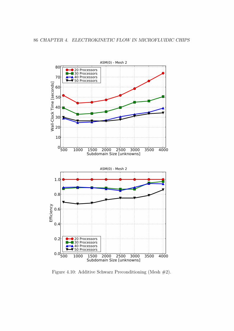
86 CHAPTER 4. ELECTROKINETIC FLOW IN MICROFLUIDIC CHIPS
500 1000 1500 2000 2500 3000 3500 4000Subdomain Size [unknowns]
0
10
20
30
40
50
60
70
80
Wall-C
lock T
ime [
seconds]
ASM(0) - Mesh 2
20 Processors30 Processors40 Processors50 Processors
500 1000 1500 2000 2500 3000 3500 4000Subdomain Size [unknowns]
0.0
0.2
0.4
0.6
0.8
1.0
Eff
icie
ncy
ASM(0) - Mesh 2
20 Processors30 Processors40 Processors50 Processors
Figure 4.10: Additive Schwarz Preconditioning (Mesh #2).

4.4. CLASSICAL DOMAIN DECOMPOSITION METHODS 87
500 1000 1500 2000 2500 3000 3500 4000Subdomain Size [unknowns]
0
50
100
150
200
250
300
Wall-C
lock T
ime [
seconds]
ASM(0) - Mesh 3
20 Processors30 Processors40 Processors50 Processors
500 1000 1500 2000 2500 3000 3500 4000Subdomain Size [unknowns]
0.0
0.2
0.4
0.6
0.8
1.0
1.2
Eff
icie
ncy
ASM(0) - Mesh 3
20 Processors30 Processors40 Processors50 Processors
Figure 4.11: Additive Schwarz Preconditioning (Mesh #3).
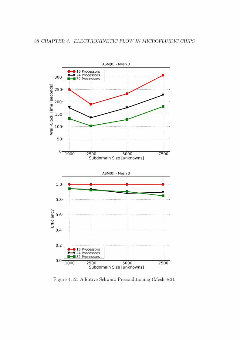
88 CHAPTER 4. ELECTROKINETIC FLOW IN MICROFLUIDIC CHIPS
1000 2500 5000 7500Subdomain Size [unknowns]
0
50
100
150
200
250
300
Wall-C
lock T
ime [
seconds]
ASM(0) - Mesh 3
16 Processors24 Processors32 Processors
1000 2500 5000 7500Subdomain Size [unknowns]
0.0
0.2
0.4
0.6
0.8
1.0
Eff
icie
ncy
ASM(0) - Mesh 3
16 Processors24 Processors32 Processors
Figure 4.12: Additive Schwarz Preconditioning (Mesh #3).
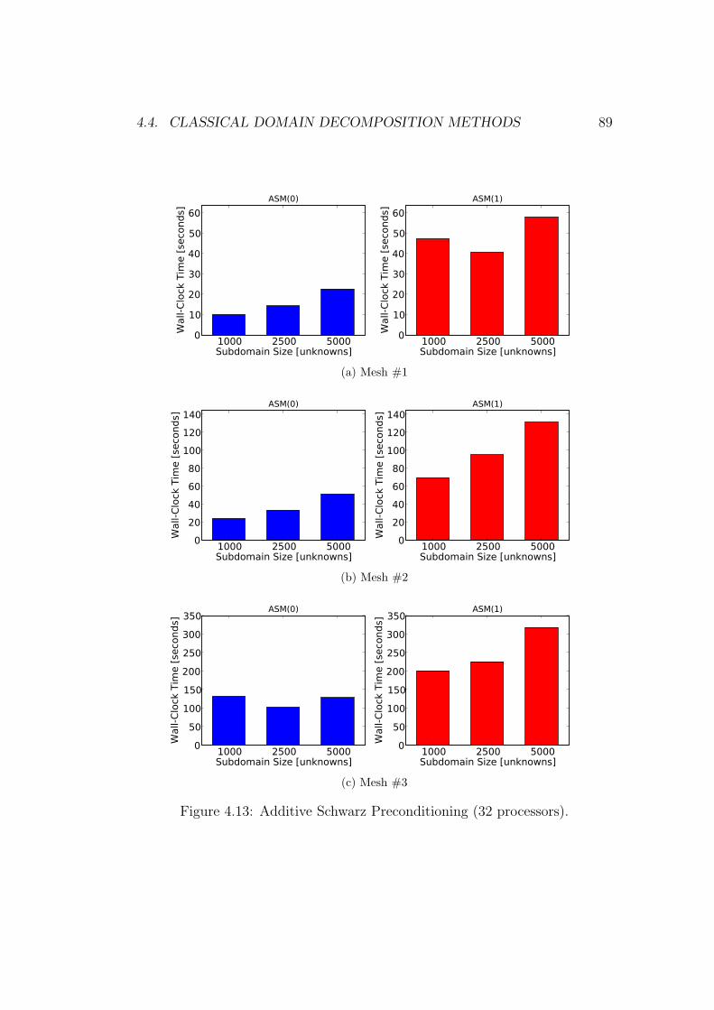
4.4. CLASSICAL DOMAIN DECOMPOSITION METHODS 89
1000 2500 5000Subdomain Size [unknowns]
0
10
20
30
40
50
60
Wall-C
lock T
ime [
seconds]
ASM(0)
1000 2500 5000Subdomain Size [unknowns]
0
10
20
30
40
50
60
Wall-C
lock T
ime [
seconds]
ASM(1)
(a) Mesh #1
1000 2500 5000Subdomain Size [unknowns]
0
20
40
60
80
100
120
140
Wall-C
lock T
ime [
seconds]
ASM(0)
1000 2500 5000Subdomain Size [unknowns]
0
20
40
60
80
100
120
140
Wall-C
lock T
ime [
seconds]
ASM(1)
(b) Mesh #2
1000 2500 5000Subdomain Size [unknowns]
0
50
100
150
200
250
300
350
Wall-C
lock T
ime [
seconds]
ASM(0)
1000 2500 5000Subdomain Size [unknowns]
0
50
100
150
200
250
300
350
Wall-C
lock T
ime [
seconds]
ASM(1)
(c) Mesh #3
Figure 4.13: Additive Schwarz Preconditioning (32 processors).


Chapter 5
Final Remarks
5.1 Impact of this work
MPI for Python and PETSc for Python were primarily conceived to be small
packages providing very basic parallel functionalities. The original intention
revolved around providing a programmable scripting interface to PETSc-FEM.
As time passed, MPI for Python and PETSc for Python progressively evolved
and gained more and more functionalities. At the time of this writing, they
had become full-featured packages able to support serious medium and large
scale parallel applications.
MPI for Python and PETSc for Python are serving the original purposes
that initially motivated their development. Currently, both packages are fully
integrated to a Python module providing access to PETSc-FEM function-
alities. However, the initial intent of providing PETSc-FEM with a pro-
grammable scripting interface was early abandoned. Using PETSc-FEM func-
tionalities directly from a Python programming environment is a much more
attractive and productive alternative. Python codes are being used for driving
PETSc-FEM parallel finite elements simulations. This software infraestruc-
ture is supporting research activities related to fluid flow in micro-channels,
fluid-structure interaction, and fluid-induced vibration.
The Synergia 3D project [68] is developed by the Advanced Accelerator
Modelling team at the Fermilab Computing Division. The software simulates
91

92 CHAPTER 5. FINAL REMARKS
the behavior of particles in an accelerator, emphasizing three-dimensional mod-
els of collective beam effects. This project uses Python-driven Fortran 90 and
C++ libraries to create beam dynamics simulations. The individual beam
dynamics libraries were designed to use MPI to support parallel computation.
MPI for Python is used from the Python-driven simulations to support com-
munication within MPI at the Python level.
MPI for Python has also been successfully employed in non-scientific appli-
cations. The Ghostscript project, a well-known and widely used interpreter for
the PostScript language, has taken advantage of MPI for Python for moving its
originally sequential and Python-based software regression testing framework–
targeted to early detect unintended behavior changes during development–to
a traditional cluster-based environment. Originally, the huge test suite took
hours to complete. After parallelization, the automated checks could be per-
formed after every source code change, returning feedback in a few minutes.
MPI for Python was chosen because it provided the best mix of the traditional
MPI features developers were familiar to and its integration with the Python
language.
Some core component of PETSc for Python have recently served as the
foundation for further developments. SLEPc for Python [69] (known in short
as slepc4py) is a recent software project providing access to to the Scalable
Library for Eigenvalue Problem Computations (SLEPc) [70, 71] for the Python
programming language. SLEPc is a software library for the solution of large
scale sparse eigenvalue problems on parallel computers; it is being developed by
the High Performance Networking and Computing Group of the Universidad
Politecnica de Valencia, Spain. SLEPc for Python is being developed at the
University of Nebraska-Lincoln, USA. The core developers of SLEPc and the
author of this thesis have also colaborated and made contributions to it.

5.2. PUBLICATIONS 93
5.2 Publications
During the work on this thesis the following articles have been published or
are going to be published in referred journals.
1. Alejandro Limache, Pablo Sanchez, Lisandro D. Dalcın, and
Sergio Idelsohn. Objectivity tests for Navier-Stokes simulations: the
revealing of non-physical solutions produced by Laplace formulations.
Computer Methods in Applied Mechanics and Engineering, In Press,
2008. doi:10.1016/j.cma.2008.04.020
2. Lisandro D. Dalcın, Rodrigo R. Paz and Mario A. Storti. MPI
for Python: performance improvements and MPI-2 extensions. Journal
of Parallel and Distributed Computing, 68(5):655-662, 2008. doi:10.
1016/j.jpdc.2007.09.005
3. Mario A. Storti, Norberto M. Nigro, Rodrigo R. Paz and
Lisandro D. Dalcın. Dynamics boundary conditions in fluid mechan-
ics. Computer Methods in Applied Mechanics and Engineering, 197(13-
16):1219-1232, 2008. doi:10.1016/j.cma.2007.10.014
4. Mario A. Storti, Lisandro D. Dalcın, Rodrigo R. Paz, An-
drea Yommi, Victorio Sonzogni, and Norberto M. Nigro. A
preconditioner for the Schur complement matrix. Advances in Engi-
neering Software, 37(11):754-762, 2006. doi:10.1016/j.advengsoft.
2006.02.003
5. Lisandro D. Dalcın, Rodrigo R. Paz and Mario A. Storti. MPI
for Python. Journal of Parallel and Distributed Computing, 65(9):1108-
1115, 2005. doi:10.1016/j.jpdc.2005.03.010
Additionally, several articles have been submitted and presented in na-
tional international conferences at Argentina on numerical methods for com-
putational mechanics.


Bibliography
[1] Beowulf.org. The Beowulf cluster site, 2008. http://www.beowulf.org/.
ix
[2] Satish Balay, Kris Buschelman, William D. Gropp, Dinesh Kaushik,
Matthew G. Knepley, Lois Curfman McInnes, Barry F. Smith, and Hong
Zhang. PETSc Web page, 2008. http://www.mcs.anl.gov/petsc. x, 40
[3] The Trilinos Team Sandia National Laboratories. The Trilinos project,
2008. http://trilinos.sandia.gov. x
[4] Satish Balay, Kris Buschelman, Victor Eijkhout, William D. Gropp, Di-
nesh Kaushik, Matthew G. Knepley, Lois Curfman McInnes, Barry F.
Smith, and Hong Zhang. PETSc users manual. Technical Report ANL-
95/11 - Revision 2.3.3, Argonne National Laboratory, 2007. x, 40
[5] Satish Balay, William D. Gropp, Lois Curfman McInnes, and Barry F.
Smith. Efficient management of parallelism in object oriented numerical
software libraries. In E. Arge, A. M. Bruaset, and H. P. Langtangen,
editors, Modern Software Tools in Scientific Computing, pages 163–202.
Birkhauser Press, 1997. x, 40
[6] Guido van Rossum. Python programming language, 1990–2008. http:
//www.python.org/. x, 1
[7] Guido van Rossum. Python reference manual. http://docs.python.
org/ref/ref.html, May 2008. x
[8] Lisandro Dalcın, Rodrigo Paz, and Mario Storti. MPI for Python. Journal
of Parallel and Distributed Computing, 65(9):1108–1115, sep 2005. xii
95

96 BIBLIOGRAPHY
[9] Lisandro Dalcın, Rodrigo Paz, and Mario Storti Jorge D’Elia. MPI for
Python: Performance improvements and MPI-2 extensions. Journal of
Parallel and Distributed Computing, 68(5):655–662, may 2008. xii
[10] Lisandro Dalcın. MPI for Python, 2005-2008. http://mpi4py.scipy.
org. xii
[11] Lisandro Dalcın. PETSc for Python, 2005-2008. http://petsc4py.
googlecode.com/. xii
[12] Mario Alberto Storti, Norberto Nigro, and Rodrigo Paz. PETSc-FEM: A
general purpose, parallel, multi-physics FEM program, 1999-2008. http:
//www.cimec.org.ar/petscfem. xii, 65
[13] Travis Oliphant. NumPy: Numerical Python, 2005–2008. http://numpy.
scipy.org/. 2
[14] Eric Jones, Travis Oliphant, Pearu Peterson, et al. SciPy: Open source
scientific tools for Python, 2001–2008. http://www.scipy.org/. 2
[15] Pearu Peterson. F2PY: Fortran to Python interface generator, 2000–2008.
http://cens.ioc.ee/projects/f2py2e/. 2
[16] David M. Beazley. SWIG: Simplified wrapper and interface generator,
1996–2008. http://www.swig.org/. 3
[17] David M. Beazley and Peter S. Lomdahl. Feeding a large scale physics
application to Python. In Proceedings of 6th. International Python Con-
ference, pages 21–29, San Jose, California, October 1997. 3
[18] K. Kadau, T. C. Germann, and P. S. Lomdahl. Molecular Dynamics
Comes of Age:. 320 Billion Atom Simulation on BlueGene/L. Interna-
tional Journal of Modern Physics C, 17:1755–1761, 2006. 3
[19] Marc Snir, Steve Otto, Steven Huss-Lederman, David Walker, and Jack
Dongarra. MPI - The Complete Reference: Volume 1, The MPI Core,
volume 1, The MPI Core. MIT Press, Cambridge, MA, USA, 2nd. edition,
1998. 6

BIBLIOGRAPHY 97
[20] William Gropp, Steven Huss-Lederman, Andrew Lumsdaine, Ewing Lusk,
Bill Nitzberg, William Saphir, and Marc Snir. MPI - The Complete Refer-
ence: Volume 2, The MPI-2 Extensions, volume 2, The MPI-2 Extensions.
MIT Press, Cambridge, MA, USA, 2nd. edition, 1998. 6
[21] Message Passing Interface Forum. Message Passing Interface (MPI) Fo-
rum Home Page, 2008. http://www.mpi-forum.org/. 7
[22] MPI Forum. MPI: A message passing interface standard. International
Journal of Supercomputer Applications, 8(3/4):159–416, 1994. 7
[23] MPI Forum. MPI2: A message passing interface standard. High Perfor-
mance Computing Applications, 12(1–2):1–299, 1998. 7
[24] MPICH Team. MPICH: A portable implementation of MPI, 2005. http:
//www-unix.mcs.anl.gov/mpi/mpich/. 7
[25] W. Gropp, E. Lusk, N. Doss, and A. Skjellum. A high-performance,
portable implementation of the MPI message passing interface standard.
Parallel Computing, 22(6):789–828, September 1996. 7
[26] Open MPI Team. Open MPI: Open source high performance computing,
2008. http://www.open-mpi.org/. 7
[27] Edgar Gabriel, Graham E. Fagg, George Bosilca, Thara Angskun, Jack J.
Dongarra, Jeffrey M. Squyres, Vishal Sahay, Prabhanjan Kambadur,
Brian Barrett, Andrew Lumsdaine, Ralph H. Castain, David J. Daniel,
Richard L. Graham, and Timothy S. Woodall. Open MPI: Goals, con-
cept, and design of a next generation MPI implementation. In Proceed-
ings, 11th European PVM/MPI Users’ Group Meeting, pages 97–104, Bu-
dapest, Hungary, September 2004. 7
[28] Institute of Electrical and Electronics Engineers. System Application Pro-
gram Interface (API) [C Language]. Information technology—Portable
Operating System Interface (POSIX). IEEE Computer Society, 345 E.
47th St, New York, NY 10017, USA, 1990. 11

98 BIBLIOGRAPHY
[29] Jeffrey M. Squyres, Jeremiah Willcock, Brian C. McCandless, Peter W.
Rijks, and Andrew Lumsdaine. OOMPI Home page, 1996. http://www.
osl.iu.edu/research/oompi/. 11
[30] Brian C. McCandless, Jeffrey M. Squyres, and Andrew Lumsdaine. Object
oriented MPI (oompi): a class library for the message passing interface.
In MPI Developer’s Conference, pages 87–94, Jul 1996. 11
[31] Patrick Miller. pyMPI: Putting the py in MPI, 2000–2008. http://
pympi.sourceforge.net/. 12
[32] Ole Nielsen. Pypar Home page, 2002–2008. http://datamining.anu.
edu.au/∼ole/pypar/. 12
[33] Konrad Hinsen. ScientificPython: Home page, 2008. http://dirac.
cnrs-orleans.fr/plone/software/scientificpython/. 12
[34] Mario Alberto Storti. Aquiles cluster at CIMEC, 2005-2008. http://
www.cimec.org.ar/aquiles. 28, 58
[35] Mario Alberto Storti. Geronimo cluster at CIMEC, 2001–2005. http:
//www.cimec.org.ar/geronimo. 35
[36] R.D. Falgout, J.E. Jones, and U.M. Yang. Numerical Solution of Partial
Differential Equations on Parallel Computers, volume 51, chapter The De-
sign and Implementation of hypre, a Library of Parallel High Performance
Preconditioners, pages 267–294. Springer-Verlag, 2006. 41
[37] Michael Heroux, Roscoe Bartlett, Vicki Howle Robert Hoekstra, Jonathan
Hu, Tamara Kolda, Richard Lehoucq, Kevin Long, Roger Pawlowski, Eric
Phipps, Andrew Salinger, Heidi Thornquist, Ray Tuminaro, James Wil-
lenbring, and Alan Williams. An Overview of Trilinos. Technical Report
SAND2003-2927, Sandia National Laboratories, 2003. 41
[38] P. R. Amestoy, I. S. Duff, J.-Y. L’Excellent, and J. Koster. A fully asyn-
chronous multifrontal solver using distributed dynamic scheduling. SIAM
Journal on Matrix Analysis and Applications, 23(1):15–41, 2001. 41
BIBLIOGRAPHY 99
[39] Steven Bernard and Marcus Grote. SPAI Web Page. http://www.sam.
math.ethz.ch/∼grote/spai/. 41
[40] Peter N. Brown and Youcef Saad. Hybrid Krylov methods for nonlinear
systems of equations. SIAM J. Sci. Stat. Comput., 11:450–481, 1990. 44
[41] M. Pernice and H. F. Walker. NITSOL: A Newton iterative solver for
nonlinear systems. SIAM J. Sci. Stat. Comput., 19:302–318, 1998. 44
[42] R. Barrett, M. Berry, T. F. Chan, J. Demmel, J. Donato, J. Dongarra,
V. Eijkhout, R. Pozo, C. Romine, and H. Van der Vorst. Templates for
the Solution of Linear Systems: Building Blocks for Iterative Methods,
2nd Edition. SIAM, Philadelphia, PA, 1994. 55
[43] Victorio E. Sonzogni, Andrea M. Yommi, Norberto M. Nigro, and
Mario A. Storti. A parallel finite element program on a Beowulf clus-
ter. Advances in Engineering Software, 33(7–10):427–443, July / October
2002. 65
[44] T. Tezduyar, S. Mittal, S. Ray, and R. Shih. Incompressible flow computa-
tions with stabilized bilinear and linear equal order interpolation velocity
pressure elements. Computer Methods in Applied Mechanics and Engi-
neering, 95:221–242, 1992. 66
[45] T.E. Tezduyar and Y. Osawa. Finite element stabilization parameters
computed from element matrices and vectors. Computer Methods in Ap-
plied Mechanics and Engineering, 190(3-4):411–430, 2000. 66
[46] D.R. Reyes, D. Iossifidis, P.A. Auroux, and A. Manz. Micro total analysis
systems. 1. introduction, theory, and technology. Analytical Chemistry,
74(12):2623–2636, 2002. 66
[47] M. Freemantle. Downsizing chemistry: Chemical analysis and synthesis on
microchips promise a variety of potential benefits. Chemical Engineering
News, 77:27–36, 1999. 66
[48] M.J. Madou. Fundamentals of Microfabrication: The Science of Minia-
turization. CRC Press, second edition, 2002. 66

100 BIBLIOGRAPHY
[49] D. Erickson and D. Li. Integrated microfluidic devices. Analytica Chimica
Acta, 507(1):11–26, 2004. 67
[50] N.A. Patankar and H.H. Hu. Numerical simulation of electroosmotic flow.
Analytical Chemistry, 70(9):1870–1881, 1998. 67
[51] F. Bianchi, R. Ferrigno, and H.H. Girault. Finite element simulation of
an electroosmotic-driven flow division at a t-junction of microscale dimen-
sions. Analytical Chemistry, 72(9):1987–1993, 2000. 67
[52] N. Sundararajan, M.S. Pio, L.P. Lee, and A.A. Berlin. Three-dimensional
hydrodynamic focusing in polydimethylsiloxane (pdms) microchannels.
Journal of Microelectromechanical Systems, 13(4):559–567, 2004. 67
[53] J.M. MacInnes, X. Du, and R.W.K. Allen. Prediction of electrokinetic and
pressure flow in a microchannel T-junction. Physics of Fluids, 15(7):1992–
2005, 2003. 67
[54] D. Erickson. Towards numerical prototyping of labs-on-chip: modeling for
integrated microfluidic devices. Microfluidics and Nanofluidics, 1(4):301–
318, 2005. 67
[55] Hunter R.J. Foundations of Colloid Science. Oxford University Press,
second edition, 2001. 68, 71, 72
[56] Probstein R.F. Physicochemical Hydrodynamics. An Introduction. Wiley-
Interscience, second edition, 2003. 68, 69, 71, 72
[57] P. Tabeling. Introduction to Microfluidics. Oxford University Press, 2005.
68
[58] Stone H.A., Stroock A.D., and Ajdari A. Engineering flows in small de-
vices: Microfluidics toward a lab-on-a-chip. Annual Review of Fluid Me-
chanics, 36:381–411, 2004. 68
[59] T.M. Squires and S.R. Quake. Microfluidics: Fluid physics at the nanoliter
scale. Reviews of Modern Physics, 77(3), 2005. 68
BIBLIOGRAPHY 101
[60] Barry F. Smith, Petter E. Bjørstad, and William Gropp. Domain De-
composition: Parallel Multilevel Methods for Elliptic Partial Differential
Equations. Cambridge University Press, 1996. 78
[61] Clark R. Dohrmann. A preconditioner for substructuring based on con-
strained energy minimization. SIAM Journal on Scientific Computing,
25(1):246–258, 2003. 78
[62] Charbel Farhat, Michel Lesoinne, Patrick LeTallec, Kendall Pierson, and
Daniel Rixen. FETI-DP: a dual-primal unified FETI method - part i: A
faster alternative to the two-level FETI method. International Journal
for Numerical Methods in Engineering, 50(7):1523–1544, 2001. 78
[63] Andreas Frommer and Hartmut Schwandt. A unified representation and
theory of algebraic additive Schwarz and multisplitting methods. SIAM
J. Matrix Anal. Appl., 18(4):893–912, 1997. 78
[64] Martin J. Gander and Laurence Halpern. Optimized Schwarz waveform
relaxation methods for advection reaction diffusion problems. SIAM J.
Numer. Anal., 45(2):666–697, 2007. 78
[65] Martin J. Gander, Laurence Halpern, and Frederic Magoules. An opti-
mized schwarz method with two-sided robin transmission conditions for
the helmholtz equation. International. Journal for Numerical Methods in
Fluids, 55(2):163–175, 2007. 78
[66] Hermann. A. Schwarz. Uber einen Grenzubergang durch alternieren-
des Verfahren. Vierteljahrsschrift der Naturforschenden Gesellschaft in
Zurich, 15:272–286, May 1870. 81
[67] George Karypis and Vipin Kumar. Multilevel k-way partitioning scheme
for irregular graphs. Journal of Parallel and Distributed Computing,
48(1):96–129, 1998. 83
[68] J. Amundson, P. Spentzouris, J. Qiang, and R. Ryne. Synergia: A 3D ac-
celerator modelling tool with 3D space charge. Journal of Computational
Physics, 211(1):229–248, January 2006. 91

102 BIBLIOGRAPHY
[69] Brian Bockelman. SLEPc for Python, 2008. http://t2.unl.edu/
documentation/slepc4py. 92
[70] Vicente Hernandez, Jose E. Roman, and Vicente Vidal. SLEPc: A scal-
able and flexible toolkit for the solution of eigenvalue problems. ACM
Transactions on Mathematical Software, 31(3):351–362, September 2005.
92
[71] Vicente Hernandez, Jose E. Roman, and Vicente Vidal. SLEPc Web page,
2008. http://www.grycap.upv.es/slepc/. 92