Contents

Foreword

FIELD TECHNIQUE

1 2 3 4 5 6 7 8 9

10 11 12 13 14 15

Plot size, shape, and orientation Number of replications Experimental design Blocking Randomization Soil heterogeneity Border effect Missing hills Replanting dead hills Residual effect of fertilizer Residual effect of unplanted alleys Number of seedlings per hill Off-types Pest and disease damage Minor sources of variation

2 4 6

10 11 14 17 20 22 23 24 25 26 27 28

COLLECTION OF DATA

16 17 18 19 20 21 22 23

Plot sampling Measuring grain yields Measuring plant height and tiller number Measuring yield components Measuring leaf area index Measuring stem borer incidence Sampling in broadcast rice Sampling for protein determination References Appendix Table 1. Random numbers Appendix Table 2. Correction factors for adjusting

grain weight to 14% moisture

32 34 35 37 39 41 42 43 44 46

48

Foreword

This manual is primarily intended for field researchers con- ducting experiments on rice. It attempts to define and provide tested solutions to all major problems of experimentation technique. Most problems discussed are common to many field experiments dealing with rice.

In an effort to be brief, direct, and clear, emphasis is placed on recommended solutions rather than on the data substanti- ating the recommendations. Whenever possible, both preven- tive and remedial measures are presented. Only substantiated procedures are recommended: untried alternatives are not included.

The manual has two parts. The first covers field plot techniques, experimental design, and sources of experimental error. The second part deals with sampling and measurement techniques for determining plot yield and other characters.

I am grateful to Mr. Steven A. Breth for editing the manuscript and for his stimulating influence; to Dr. S.K. De Datta for his invaluable assistance in the conduct of actual field experiments from which data presented here were gath- ered; to Mr. Federico Gatmaitan. Jr. and Mr. Arnulfo del Rosario for preparing the illustrations; and to the staff of the department of statistics for the collection and analysis of data.

KWANCHAI A. GOMEZ

2 Field technique

PLOT SIZE, SHAPE, 1 AND ORIENTATION

Experimental plot refers to the unit on which random assign- ment of treatments is made. The size of the plot, therefore, refers not only to the harvest area but to the whole unit receiving the treatment. The shape of the plot refers to the ratio of its length to its width. The orientation of plots, on the other hand, refers to the choice of direction along which the lengths of the plots will be placed. The orientation of plots naturally is not defined for square plots.

Effects of plot size, shape, orientation. The size, shape, and orientation of a plot can greatly affect the magnitude of experi- mental error in a field trial. Too small plots may give unreli- able results; unnecessarily large plots waste time and re- sources. A square plot, with its minimum perimeter, exposes the smallest number of plants to border effects. Orientation of plots can reduce or increase the effects of fertility gradients in the field.

In general, experimental error decreases as plot size in- creases, but the reduction is not proportional.

Plot size not only affects variability but may also bring about bias in the experimental results. Plots should be wide enough to permit the removal of border rows when necessary (see chapter 7 for details on border effects).

For a specified area of land, the number of replications de- creases as the plot size is increased. Consequently a gain in precision from increased plot size is accompanied by a loss of precision from reduced number of replications (see chapter 2 for details on number of replications). But in general, as long as the minimum plot size is reached, a larger increase in precision can be expected with an increase in number of replications.

How to choose plot size, shape, orientation. In rice field ex- periments, plots commonly range from 8 to 25 sq m. Whatever size and shape of plots you choose, make sure that an area not smaller than 5 sq m, free from all types of competition and border effects, is available for harvesting and determining plot yield. Consider the following when choosing plot size and shape.

Plot size, shape, and orientation 3

Relation of coefficient of variation to plot size based on rice yield data from two uniformity trials.

Type of experiment. The cultural practices related to the experiment can dictate the size and shape of plots for ease of operations. Fertilizer trials require larger plots than variety yield tests. Irrigation studies may require even larger plots. In insecticide or herbicide trials where the chemicals are to be sprayed, the width of the plot may be governed by the range of coverage of the sprayer used.

Soil heterogeneity. When soil heterogeneity is patchy (that is, when correlation between productivity of adjacent areas is low), a large plot should be used. The choice of plot shape is not critical when soil variation is as great in one direction as it is in another. On the other hand, if a gradient is present, plots should have their longest dimension in the direction of great- est variation. Therefore when the fertility gradient of the experimental field is known, a rectangular plot with appropri- ate orientation will give higher precision (see chapter 6 on orienting plots to reduce the effects of soil heterogeneity). But when the fertility pattern of the area is not known it is safer to

4 Field technique

use square plots (they will not give the best precision, nor will they give the worst).

Border effects. In experiments where border effects might be appreciable, square plots are desirable because they have minimum perimeter for a given plot size. In varietal yield tests where varietal competition is expected, plots with at least six rows should be used to allow exclusion of one row on each side of the plot, thus leaving four center rows for harvest.

Scarcity of seeds. When the seed supply is limited (as in early generations of crosses), you may have to use very small plots. Two points should be kept in mind. First, consider the magnitude of the difference in plant characters among the test selections. If characters like plant height, tillering capacity, or growth duration differ greatly, the effect of varietal competi- tion can not be properly controlled in very small plots. Thus, bias may enter into the results. Second, a very refined field technique is essential to ensure accuracy because, with small plots, small errors often are greatly magnified. When small plots are needed, you must be willing to bear the higher costs that result from using a more refined technique than the techniques generally used with large plots.

Measurement of characters other than yield. When several plant characters are to be measured, you may need extra plants for sampling, especially when the measurement requires the destruction of plants at early growth stages as in the determi- nation of dry matter production or leaf area index. Provide a large enough area to ensure against plant competition which could result when sample plants are pulled out (see chapter 16).

2 NUMBER OF REPLICATIONS

How often a complete set of treatments is repeated in an experiment is called the number of replications. Several quadrats (small harvest cuts) sampled from a large area planted to a variety, or multiple observations from a plot, do not represent a true replication. They are subsamples and their variability constitutes a sampling error instead of an experi- mental error. This distinction is missed by many agricultural researchers.

Number of replications 5

Effect of replication. Replication is required in an experi- ment to provide a measure of experimental error. Moreover, one of the simplest means of increasing precision is increasing the number of replications. Beyond a certain number of replications, however, the improvement in precision is too small to be worth the additional cost. When such a point is reached and the required precision is still not attained, other means besides increasing the number of replications must be used.

How to determine number of replications. The number of replications you need depends on the magnitude of experi- mental error likely to be obtained in the experiment and the degree of precision you want.

The magnitude of experimental error in an experiment is generally prescribed as the value of coefficient of variation based on the most important character (usually yield) likely to be obtained in the experiment. The level of the coefficient of variation likely to be obtained varies from one experiment station to another and from one type of experiment to another. At the IRRI experimental farm, the average coefficient of variation based on grain yield is about 8 percent for varietal yield tests and 10 percent for other agronomic trials. At other localities, the level of the coefficient of variation may be different from the level at IRRI depending upon the degree of soil heterogeneity in the experimental fields and the type of field plot technique employed.

The degree of precision desired is generally prescribed either as the standard error of the treatment means, or as the magnitude of treatment difference that can be detected.

Four replications are commonly used in rice field experi- ments at IRRI. The number of replications you need may differ greatly from this figure. Tables 1 and 2 show how many

Replications Standard error (%) Table 1. Estimated stan- dard error of a treatment (no.)

cv = 8% cv = 10% cv = 12%

2 5.7 7.1 8.5 3 4

4.6 5.8 4.0 5.0

6.9

5 6.0

6 3.6 4.5 3.3

5.4 4.1 4.9

7 3.0 3.8 8

4.5 2.8 3.5 4.2

cv = 14% mean as a percentage of the mean for varying

9.9 number of replications and coefficients of vari-

7.0 ation (cv). 6.3 5.7 5.3 5.0

8.1

6 Field technique

Table 2. Estimated per-

tween two treatment centage difference be-

tected with 95% confi- means that can be de-

dence for varying number of replications and coeffi- cients of variation (cv).

Replications Detectable difference (%) (no.)

2 18.1 22. 6 27.1 3

31.7 13.7 17.2

4 11.6 14. 5 17.4 20.6 24.0

20.3 5 6

10.3 9.3

12.9 15.4 11.6

18.0 14.0

7 16.3

8.6 8 8.9

10.7 12.9 10.0 12.0

15.0 14.0

CV = 8% CV = 10% CV = 12% CV = 14%

replications to use for a prescribed degree of precision under the magnitude of experimental error likely to be encountered in your experiment. For example, if the experiment is likely to have about 10 percent coefficient of variation, you need four replications to obtain a treatment mean with a standard error of not more than 5 percent. With four replications and a coefficient of variation of 10 percent, you can expect to detect, with 95 percent confidence, any difference between two treatment means equivalent to 13.5 percent of the mean value. With a mean yield of 6 t/ha, the detectable difference of 14.5 percent implies an amount of 0.9 t/ha. That is, with four replications and a coefficient of variation of 10 percent, you can expect to detect differences of not less than 0.9 t/ha between treatment means.

In addition to the above consideration, you must also make sure that the number of replications you choose will provide not less than 10 degrees of freedom for estimating experimen- tal error. For example, with three treatments in a randomized complete block design, four replications are not sufficient because they provide only six degrees of freedom for error. When in doubt consult a statistician.

3 EXPERIMENTAL DESIGN

Experimental design refers to the rules regulating the assign- ment of treatments to the experimental plots. Properly done it allows valid comparisons among treatments and it controls the principal source of variation infieldexperiments-soil hetero- geneity.

A proper experimental design must include replication, randomization, and error control.

Experimental design 7

Choosing a design. The best type of design for an experiment depends primarily on the magnitude of soil heterogeneity in the test area, the type and number of treatments to be tested, and the degree of precision desired. When you start a new experiment, consult a competent statistician, when possible, for a proper design to ensure that the objectives of the experiment will be met.

Do not choose a design lacking any of the three principles: replication, randomization, and error control.

Three groups of designs are commonly used in rice field experiments: complete block designs, incomplete block de- signs, and split-plot designs.

Complete block designs are generally used for simple experiments involving a small number of treatments. Some characteristics of these designs are that all treatments appear in a block, analysis of data is simple, missing data are easy to handle, and these designs can be used for either single-factor or factorial experiments.

Incomplete block designs are generally used for experi- ments that have such a large number of treatments that all treatments cannot fit into homogeneous blocks. An example is varietal tests which usually involve many varieties or selections. Some properties of such designs are that not all treatments appear in the same block and data analysis is more complicated than for complete block designs-especially with missing data. These designs can be used for either single- factor or factorial experiments.

Split-plot designs are used only for factorial experiments, either when a large number of treatment combinations is involved or when certain treatments require a larger plot size than others.

When statistical assistance is not available, the rules of thumb given below for choosing an experimental design for a single-factor or for a factorial experiment may be helpful.

SINGLE-FACTOR EXPERIMENTS

Complete block designs Randomized complete block (RCB)

less than 10 treatments any number of replications is possible uni-directional fertility gradient in the area

8 Field technique

Latin square (LS) four to eight treatments number of replications same as number of treatments bi-directional fertility gradient in the area

Incomplete block designs Balanced lattice

large number of treatments number of treatments is a squared value, say, p 2

number of replications is p + 1 number of plots per block is p (thus if, for example, number of treatments, p 2 , is 36, the number of replications, p + 1 , must be 7, and the number of plots per block, p, must be 6) same precision for all comparisons between pairs of treatments

Partially balanced lattice large number of treatments number of treatments is a squared value, say, p 2

any number of replications is possible number of plots per block is p (thus if, for example, the number of treatments p 2 , is 36, any number of replica- tions may be used, but the number of plots per block, p, must be 6) some pairs of treatments will have higher precision than others

FACTORIAL EXPERIMENTS

Complete block designs

less than 10 treatment combinations any number of replications is possible uni-directional fertility gradient in the area main effects and interactions equally important

treatment combinations between four and eight number of replications same as number of treatment

bi-directional fertility gradient in the area main effects and interactions equally important

Randomized complete block (RCB)

Latin square (LS)

combinations

Experimental design 9

Incomplete block designs Balanced lattice

large number of treatment combinations number of treatment combinations is a squared value,

number of replications is p + 1 number of plots per block is p (thus if, for example, the number of treatment combinations, p 2 , is 36, the number of replications, p + 1, must be 7, and the number of plots per block, p, must be 6) same precision for all comparisons between pairs of treatment combinations

say, p 2

Confounding more than two factors involved accuracy on certain high-order interactions can be sac- rificed

Split-plot designs Split-plot

at least two factors involved the factors are not equally important the main effect of one (or more) of the factors is less important than the other; this factor will be assigned to the main plots one factor (say, fertilizer or water management) may re- quire larger area than that of the subplot used; this factor will be assigned to the main plots

Split-split plot at least three factors involved the factors are not equally important the least important factor is assigned to main plots, the moderate one to subplots, and the most important one to sub-subplots one (or more) of the factors may require larger area than that of the subplot used

Strip-plot at least two factors involved the factors require areas larger than the size of subplot

interaction effect more important than main effects used

10 Field technique

4 BLOCKING

Blocking refers to the assignment of a group of plots or treatments to a block of land with relatively homogeneous soil. It is one of the simplest and most effective ways of coping with soil heterogeneity.

Effect of blocking. The variation among blocks can be removed from the experimental error through blocking; thus error is reduced and the precision of an experiment is in- creased. The larger the differences among blocks, the greater the reduction in the experimental error. Hence, proper block- ing should produce large differences among blocks, leaving plots within a block more homogeneous.

How to use blocking. When the fertility pattern of the experimental field is known, orient the blocks so that soil differences between blocks are maximized and those within blocks are minimized. For example, for a field with a uni- directional fertility gradient along the length of the field, blocking should be made across the width of the field, that is, cutting across or perpendicular to the gradient.

When fertility pattern is not known, avoid using long and narrow blocks. Instead, use blocks that are as compact, or as nearly square, as possible since plots that are closer can be expected to be more alike than those that are farther apart.

Conduct all management operations and data collection “on a per-block basis” to control any variation that may occur in the management and operation processes as well as in the datacollection. In other words, whenever a source of variation

Schematic diagram of a

gradient. uni-directional fertility

Randomization 11

When the fertility pattern of the field is not known, blocks should be as nearly square as possible.

exists, attempt to have the major portion of the variation separated by blocks.

For instance, when an operation (for example, application of treatments, measurement of data) can not be completed for the whole experiment in 1 day, at least complete the work for all plots in a block. In this way, the difference, if any, from day to day can be controlled by “blocking.”

The same technique can be used to handle variation among operators. Whenever an operation is known to be affected by the operator (for example, application of fertilizer or insecti- cide, measurement of plant height), each operator should be assigned to different blocks.

RANDOMIZATION 5 Randomization is one of the basic principles of experimental design. It makes valid the estimate of experimental error which is essential for comparing treatments. It is a procedure for allocating treatments so that each experimental plot has the same chance of receiving any treatment.

12 Field technique

Locating a starting point in the table of random numbers.

How to randomize. The process of randomization can be done with a table of random numbers or by drawing lots. The use of both methods is shown below for randomization and laying out of plots in a randomized complete block design with six treatments and four replications.

Random number table. First, locate a starting point in a table of random numbers (Appendix Table 1). Do this by pointing to a number in the table with your eyes closed. Use this number as the starting point. On a piece of paper write six consecutive three-digit numbers beginning at the starting point and read- ing to the right or downward.

For example, starting at the intersection of the sixteenth row and the twelfth column read downward vertically to get six three-digit numbers:

Sequence 918 1 772 2 243 3 494 4 704 5 549 6

Randomization 13

Second, rank the selected numbers from the smallest to the largest. Thus continuing the example:

Sequence Rank 918 1 6 772 2 5 243 3 1 494 4 2 704 5 4 549 6 3

Third, use the rank as the treatment number and use the sequence in which the treatment numbers occurred as the plot number in the block to which the corresponding treatment will be assigned. Thus in this example, assign treatment no. 6 to the first plot, treatment no. 5 to the second, treatment no. 1 to the third, treatment no. 2 to the fourth, treatment no. 4 to the fifth, and treatment no. 3 to the sixth.

The layout of the first block:

Fourth, repeat the first three steps for Block II, then for Block III, and finally for Block IV.

Drawing lots. First, write the numbers 1 to 6 (there are six treatments) on six equal-sized pieces of paper. Fold and place them in a box.

Second, shake the box to ensure thorough mixing of the slips of paper: then pick out one slip of paper. Write down the number and, without returning the slip of paper already taken, pick out the second slip of paper. Repeat the process until all the six pieces of paper are taken out.

14 Field technique

For example, the numbers written on the slips of paper may appear in this sequence:

Sequence 1 2 3 4 5 6

Number on paper 4 2 1 5 6 3

Third, assign the six treatments to the six plots in the first block by using the number on paper as the treatment number and the sequence as the plot number in the block.

The layout of the first block is, therefore:

Fourth, repeat the first three steps for Block II, then for Block III, and finally for Block IV.

6 SOIL HETEROGENEITY

Soil heterogeneity refers to the non-uniformity of soil from one part of the field to another. Even within a small area, soil can vary greatly in texture, drainage, moisture, and available nutrients. This variability is generally present even in a field that seems uniform. Uniformity trials at IRRI’s experimental farm have shown considerable variation in rice yields from one part of a field to another. The more common type of soil heterogeneity in a lowland rice field is a gradual change in productivity from one side of the field to the other, rather than patchy differences in productivity.

Soil heterogeneity 15

Fertility contour maps of grain yield of rice from uniformity trials in two fields at the IRRI experi- mental farm. Yields in each field range from about 5.8 to 9.3 t/ha.

Effect of soil heterogeneity. Soil heterogeneity is a major contributor to error in field experiments. It introduces a degree of uncertainty into inferences made from yield data of crops. If not properly controlled, it increases experimental error and thus lowers the precision of experimental results.

Minimizing soil heterogeneity. Some ways to minimize soil heterogeneity:

¢ Avoid areas that have been previously used for experi- ments involving treatments that may have a differential effect on soil conditions. Treatments involving fertilizer, varieties varying in growth duration, or different plant spacings may have such an effect. In such areas, one or more uniform plantings should precede an experimental planting. If you must use the area immediately, choose a design that allows for additional “blocking” based on the treatments used in previ- ous experiments (see chapter 10).

16 Field technique

Avoid areas in which alleys were left unplanted be- tween plots in the previous crop. In such areas, one or more uniform plantings should precede experimental planting. If you must use the area immediately, keep the size and location of unplanted alleys fixed in succeeding experiments (see chapter 11).

Choose areas where the history of the land use is avail- able. Such information may help you identify the possible causes of added heterogeneity from previous croppings so that appropriate remedies can be made.

If possible, conduct a uniformity trial in the prospective experimental area; that is, plant the whole area with a single variety of the crop and use uniform cultural and management practices. Uniform planting will help reduce the heterogene- ity of the soil somewhat, and the uniformity yield data (data from harvests of small units throughout the area) can be used to describe the soil heterogeneity pattern of the area for proper orientation of plots and blocks (see below) in succeeding experiments conducted in this area and to increase the preci- sion of these experiments by the use of covariance technique.

Reducing the effects of soil heterogeneity. While little can be done to eliminate or reduce soil heterogeneity itself, proper experimental techniques can considerably reduce the effects of soil heterogeneity on experimental results.

Choose proper experimental design. Choose an experi- mental design with appropriate blocking, either a complete or an incomplete block arrangement, to fit the pattern of soil heterogeneity. For instance, with a moderate number of treat- ments, a randomized complete block design can be used to take care of uni-directional fertility gradient in the area; a Latin square design can be used for a bi-directional gradient (see chapter 3 for details on experimental design).

Choose proper plot size and shape. Choose the size and shape of plot that minimizes the effect of soil heterogeneity. For instance, use a relatively larger plot for the patchy type of soil heterogeneity (that is, when correlation between produc- tivity of adjacent areas is low); use a square plot when the fertility pattern of the area is unknown (see chapter 1 for details on choice of plot size and shape).

Properly orient plots and blocks. Position the blocks so that soil differences between blocks are maximized and plots

Border effect 17

Orienting plots within a block to reduce the effect of a uni-directional fertil- ity gradient.

within the same block are as uniform as possible (see chapter 4 for blocking technique). On the other hand, arrange the plots so that the variation among plots within the same block is small. Orient the plots so that each covers the direction of the greatest variation in the block (see chapter 1 for information on orientation of plots).

Increase number of replications. For the same degree of precision, more replications are required with heterogenous soil than with homogeneous soil.

BORDER EFFECT 7 A border effect is the difference in performance between plants along the sides or ends of a plot and those in the center. It occurs when an unplanted space is left between adjacent plots or at the end of plots, when adjacent plots are planted with different varieties, or when adjacent plots have different fertilizer treatments. It influences many agronomic characters including yield (only yield data are presented below).

Effect of unplanted borders. When plots are adjacent to unplanted borders, plants in the outermost row (that is, the first row bordering unplanted space) give higher yields than those in the center. Occasionally the yield may be increased by more than 100 percent (Table 3). On the other hand, yields of the second row may be decreased. A yield reduction in the second row can be expected when fertility is high or when the

18 Field technique

Table 3. Grain yield of rows of IR8 bordering Yield (t/ha) unplanted borders of dif- Width of the ferent widths, under two unplanted 0 kg/ha N 120 kg/ha N fertilizer treatments. IRRI, space (cm) 1969 dry season. Row Row Center Row Row Center

1 a 2 rows 1 2 rows

40 60 6.91 ** 4.35 4.28 11.53 ** 5.81 6.20

10 0 9.12 ** 4.39 4.38 13.35 ** 6.24 * 7.09

6.01 * 4.08 4.12 9.69 ** 6.31 6.88

*Significantly different from the center rows at the 5% level. **Significantly different from the center rows at the 1% level. a Row 1 refers to the outermost row and row 2 to the second outermost row

Table 4. Grain yield of rows of IR8 bordering IR127-80-

fertilizer treatments. IRRI, Row 1 and Peta, a under two

1969 dry season.

Yield (t/ha)

Bordering IR127-80-1 Bordering Peta

0 kg/ha N 120 kg/ha N 0 kg/ha N 120 kg/ha N

1 4.91 ** 6.33 3.36 ** 4.58 ** 2 3

3.95 5.83 3.70 4.88 ** 3.87 5.93 3.74 5.21 *

Center rows 4.04 5.89 4.04 5.89

*Significantly different from the center rows at the 5% level. **Significantly different from the center rows at the l% level a IRE is short and high-tillering. lR127-80-1 is medium-short and low-tillering: Peta is tall and medium-tillering

unplanted space is wider than 60 cm (the discussion in this chapter refers to a row distance of 20 cm).

Effect of varietal competition. When adjacent plots are planted to varieties differing in plant height, tillering ability, or growth duration, one or two border rows are generally affected depending upon the characters that differ and the magnitude of their differences (Table 4). Higher tillering or taller varieties tend to suppress the yield of border rows in adjacent plots. When varieties with different growth durations are grown side-by-side, border rows of the variety with the shorter growth duration tend to have higher yields than rows in the center of the plot. The effect of varietal competition may reach the third row if the adjacent plants lodge.

Effect of fertilizer competition. When adjacent plots receive different fertilizer treatments, border effects can be expected if plots are not separated by a levee (bund). Even immobile nitrogen fertilizer applied before transplanting may be moved

Border effect 19

Table 5. Effect of move- Grain yield (t/ha) ment of transplanters and

lncomlng side a Outgoing side b Check c fertilizer competition in orientation of plot rows on

unfertilized IR8 plots. IRRI,

Row

1 8.59** 6.91 2 4.98 4.58 3

4.36

4 4.86 4.12 4.54 4.52

5 3.97 4.32

4 68 3.73 4.36

6.31 1969 dry season.

**Significantly different from the check at the 1% level. a Side of the plot first reached by transplanters coming from an adjacent fertilized (120 kg ha N) plot. b Side opposite incoming side. c Adjacent to unfertilized plot

from one plot to another as transplanters pass through the field (Table 5).

Preventing or minimizing border effects. Border effects can be avoided or minimized in several ways.

Avoid the use of all unplanted alley to separate experi- mental plots. If an unplanted alley is needed, it should not be wider than 40 cm.

Because unplanted borders around an experiment are generally wider than those between plots, plant a few rows of a uniform border variety around the perimeter of an experi- ment to minimize the effect of unplanted borders on plots located along the sides of the field.

When varieties to be tested vary greatly in plant height, tillering ability, or growth duration, choose an experimental design that groups homogeneous varieties, particularly by height. This will reduce the number of rows needed as borders against varietal competition effect.

Construct a levee (bund) between plots receiving differ- ent fertilizer treatments.

If transplanters move from a fertilized to unfertilized plot, they may inadver- tently move some of the fertilizer.

20 Field technique

If fertilizer is applied before transplanting, avoid plac- ing plots receiving widely different fertilizer levels along the path of transplanters.

Coping with border effects. Do not measure agronomic characters, grain yield, or yield components from border rows that are likely to have border effects. How many rows to exclude depends on the type of border effects. When in doubt and when the plot size is large enough, exclude at least two border rows (or two end hills) or a 30-cm area on each side of the plot.

8 MISSING HILLS

In transplanted rice, a missing hill refers to the spot where a hill of transplanted seedlings died before maturity.

Effects of missing hills. The presence of a missing hill means that not all hills in the plot have been subjected to the same plant spacing and plant competition. In experimental plots, rice plants immediately adjacent to a missing hill perform differently than normal hills (hills surrounded by living hills). These hills generally grow more vigorously and yield more than normal hills. The magnitude of yield increase or the degree of yield compensation, however, differs with variety, plant spacing, fertility level, and crop season (Table 6).

Thus, the occurrence of missing hills poses two major problems: How to determine yield of plots with one or more

Table 6. Percentage in- crease in grain yield of hills Yield increase (%) surrounding a missing hill, Distance from for two varieties, two plant the missing spacings, and two fertil- hill (cm) izer treatments. IRRI, 1970.

IR22 lR127-80-1

0 kg/ha N 120 kg ha N 0 kg/ha N 120 kg/ha N

Dry season 20 39** 40** 17** 26** 25 23** 22** 19** 19**

Wet season 20 29** 18** 28** 21** 25 25** 8 19** 10

** Significant at the 1% level.

Missing hills 21

Missing hill.

missing hills, and whether to treat plants adjacent to a missing hill as normal hills in sampling for agronomic characters.

Coping with missing hills. If a missing hill occurs, do not measure grain yield, yield components, or any agronomic character from the four hills immediately adjacent to the missing hill. That is, harvest only hills surrounded by living hills and adjust grain weights to allow for the difference in the number of harvested hills. For example, if 95 hills were harvested instead of 100 hills, the grain weight of these 95 hills is multiplied by 100/95 (or 1.0576) to obtain the plot yield.

If the reduction in the number of hills due to the presence of missing hills in any plot is more than 20 percent of the total number of hills to be harvested in a normal plot, do not determine plot yield and regard it as "missing data" in the statistical analysis.

Minimizing missing hills. Several practices can reduce the percentage of missing hills that occur in rice experimental

Level the field thoroughly. This practice ensures a uniform water level which prevents killing of hills with too much or too little water.

Handle the seedlings with care. When pulling seedlings from the seedbed, exercise great care to minimize damage to the seedlings, especially from wilting. Keep the roots of seedlings waiting to be transplanted thoroughly buried in mud.

Use young and healthy seedlings. Discard weak and damaged seedlings at transplanting. For the ordinary wetbed nursery, 18-day-old or 21-day-old seedlings should be trans- planted. The use of too young or too old seedlings can result in a high mortality rate.

plots.

22 Field technique

Use trained transplanters. Untrained transplanters tend to break seedlings while transplanting and are generally not able to maintain a uniform depth of planting.

Protect plants against pests and diseases. Many missing hills are caused by pest and disease infestation.

Replant dead hills. To be effective, replanting must be done properly (see chapter 9).

9 REPLANTING DEAD HILLS

To reduce the percentage of missing hills in experimental plots, dead hills are generally replanted. Questions that are commonly raised: Does the replanted hill perform normally? For how long should replanting be carried out? What type of replanting material should be used?

Effect of replanting. Regardless of when the replanting is done or what type of replanting material is used, replanted hills perform differently from normal hills. The grain yield of the replanted hill is lower than that of the normal hills, even if replanting is done as early as 5 days after transplanting (Table 7). The later the replanting is done, the higher the reduction in yield. For best results use plants thinned from border hills for replanting. Replanting with seedlings taken from the original seedbed gives poor results.

Purpose of replanting. Since replanted hills perform differ- ently from normal hills, they can not be included in the harvest

Table 7. Grain yield of a replanted hill (variety IR5) Yield (g/hill) as compared with the nor- Replanting mal hills (fertilized), for (days after Seedlings from Seedlings left Seedllngs different times of replant- transplanting) original at ends thinned from ing and different sources seedbed of rows border hills of replanting material. IRRI, 1971 dry season. 5

7 20.5** 21.0**

21.6** 24.1* 21.2** 25.0

9 21.1** 22.0** 9.7** 6.9**

18.3** 22.9** 11.4**

3.2** 6.0** 9.2**

13 15 23

26.4

15.8

Normal hills 27.3 26.5 28.2

*Significantly different from the normal hills at the 5% level. **Significantly different from the normal hills at the 1% level.

Residual effect of fertilizer 23

or in the measurement of any agronomic character. But replanting, if done properly, can protect the surrounding hills. that is, it keeps surrounding hills from performing abnor- mally. On the other hand, if dead hills are not replanted, the surrounding hills will be affected and hence must be excluded from harvest (see chapter 8). Thus replanting dead hills greatly minimizes the reduction in the number of hills har- vested.

Recommended procedure for replanting. All hills that die earlier than 3 weeks after transplanting should be replanted to keep the performance of the surrounding hills normal.

For replanting material, use plants thinned from border hills, especially those bordering an unplanted space. Where thinning from border hills does not provide sufficient replant- ing material, use seedlings left in bunches at the ends of rows. Each bunch should not contain more than 10 to 15 seedlings.

Mark all replanted hills and exclude them from measure- ments of grain yield, yield components, and agronomic char- acters.

RESIDUAL EFFECT OF FERTILIZER 10 Residual effect of fertilizer refers to the effect, on the current crop, of fertilizer applied to previous crops.

Influence of residual fertilizer. The residual effect of fertil- izer can greatly affect yields. In one experiment at the IRRI farm a 13 percent increase in yield was caused by the applica- tion of 120 kg/ha of nitrogen to the previous crop (Table 8). If not properly controlled, the residual effect of fertilizer may cause bias in the experimental results and increase the magni- tude of experimental error.

preceding seasons Grain yield Plant ht Panicles Filled grains Nitrogen applied

(kg/ha) (t/ha) (cm) (no./hill) (no./panicle)

0 3.64 73.9 9.3 62.8 3.75 74.0 4.10

9.5 75.0 10.1

62.9 68.2

60 120

Table 8. Performance of IR22 plants (unfertilized)

with different nitrogen grown in areas fertilized

rates in two preceding seasons. IRRI, 1971 dry season.

LSD (5%) 0.32 n.s. n.s. 4.6

24 Field technique

avoid residual effect of Example of blocking to

fertilizer. Fertilizer trial in previous seasons had four rates of nitrogenarranged in a randomized complete block design with four replications. For an experi-

son, involving four treat- ment in the current sea-

ments, the previous rates of fertilizer application can be used as the bases for double grouping in con- junction with a latin square design.

Preventing residual effect of fertilizer. Several things can be done to prevent residual effect of fertilizer. Avoid using fields that were used forafertilizer trial in the previous season. If possible, iet the soil dry out before planting the succeeding crop. To improve soil uniformity, grow a unifonn crop with close spacing and a low fertilizer level.

Coping with residual effect of fertilizer. If you must use the problem area immediately, choose an experimental design that allows for additional “blocking” based on the levels of nitrogen applied in the previous season.

RESIDUAL EFFECT OF 11 UNPLANTED ALLEYS

In rice experiments, it is not uncommon for plots to be separated by unplanted alleys. These alleys facilitate the application of certain treatments and the gathering of data. At times the alleys may also reduce the effects of interplot competition. But plants grown in previously unplanted areas may perform differently from those grown on a continually cropped area. This phenomenon is referred to as residual effect of unplanted alleys.

Influence of residual effect of unplanted alleys. Plants grown in previously unplanted areas perform better than those grown in continually cropped areas (Table 9). Hence, un- planted alleys are a possible source of additional soil variabil-

Number of seedlings per hill 25

Grain yield Table 9. Performance of

Type of area Plant ht Panicles IR22 grown on previously

(t/ha) (cm) (no. hill) planted and unplanted

Previously unplanted areas. IRRI, 1970 dry sea-

7.41 89.1 15.5 Previously planted 6.42 88.0 14.0

son.

Difference 0.99** 1.1* 1.5**

*Significant at the 5% level. **Significant at the 1% level

ity and, hence, of additional error for experiments in succeed- ing crops.

Minimizing residual effect of unplanted alleys. In experi- mental fields that are to be cropped successively avoid separating plots with unplanted alleys. One way is to lay out the plots so they are next to each other without an alley in between. Because interplot competition may be higher when plots are immediately next to each other the plot size can be increased to provide one or two extra rows as borders. Another way to eliminate unplanted alleys is to plant a common variety between all plots. The variety planted between plots will serve as a marker to visually separate adjacent plots.

When unplanted alleys have been used in the previous season, make a uniform planting if possible in the whole area with close spacing and low fertilizer level for at least one crop season before conducting any experiment there.

If you cannot avoid using unplanted alleys and the area is also needed for immediate planting, keep size and location of the alleys fixed in succeeding experiments.

NUMBER OF SEEDLINGS PER HILL 12 Rice researchers use varying number of plants per hill, except when they want to measure tillering capacity (for which one plant per hill is necessary). They often ask, however: (1) Does it matter if a varying number of plants per hill is used in an experiment? (2) If the same number of plants per hill should be used throughout the experiment, what is the optimum number?

Effect of variable number of plants per hill. Grain yield and many yield components vary with the number of plants per hill (Table 10). Thus, the use of a variable number of plants per hill

26 Field technique

Table 10. Grain yield and yield components of Plants Yield Panicles Filled Unfilled Panicle

IR127-80-1 (90kg/ha N) as (no./hill) (t/ha) (no./hill) (no /panicle) (%) (cm) grains grains length

affected by the number of plants per hill. IRRI, 1971 wet season. 1 2.87 4.4 161

2 45.7 22.0

3.52 3

5.8 146 43.3 21.6 2.93 5.9 110 45.9 20.6

4 3.56 8.0 108 34.3 6

19.5 3.76 7.4 116 36.1 19.5

LSD (5%) 0.52 1.5 24 n.s. 1.3

Table 11. Percentage of missing hills as affected by the number of plants per hill. IRRI, 1971 dry sea- Plants son. (no./hill)

Missing hills (%)

0 kg/ha N 120 kg/ha N

lR127-80-1 lR844-86-1 lR127-80-1 lR844-86-1 Mean a

1 27.1 13.8 24.3 2

11.9 19.3 a 16.6 11.9 13.3 7.1 12.2 b

3 11.8 8.8 14.2 5.1 10.0 b 4 8.8 10.1 8.3 2.2 7.3 c 6 6.4 11.4 7.2 1.8 6.7 c

a Any two means followed by the same letter are not significantly different at the 5% level.

in a plot can be expected to increase the variability among hills, thereby requiring a larger sample size for measuring various rice characters.

Recommended number of seedlings per hill. Unless tiller- ing capacity is to be assessed. avoid using one plant per hill since it gives a very high occurrence of missing hills (Table 11). In general, use two to four seedlings per hill. Plant the same number of seedlings per hill throughout the whole experiment.

13 OFF-TYPES Off-types are plants whose genotypes differ from those of the majority of plants in the plot. They result from unpurified seed stocks or from volunteer plants that sprout from seeds dropped from the previous crop.

Effect of off-types. The presence of off-types increases heterogeneity among plants in a plot and introduces undesir- able plant competition. Since their presence is usually de-

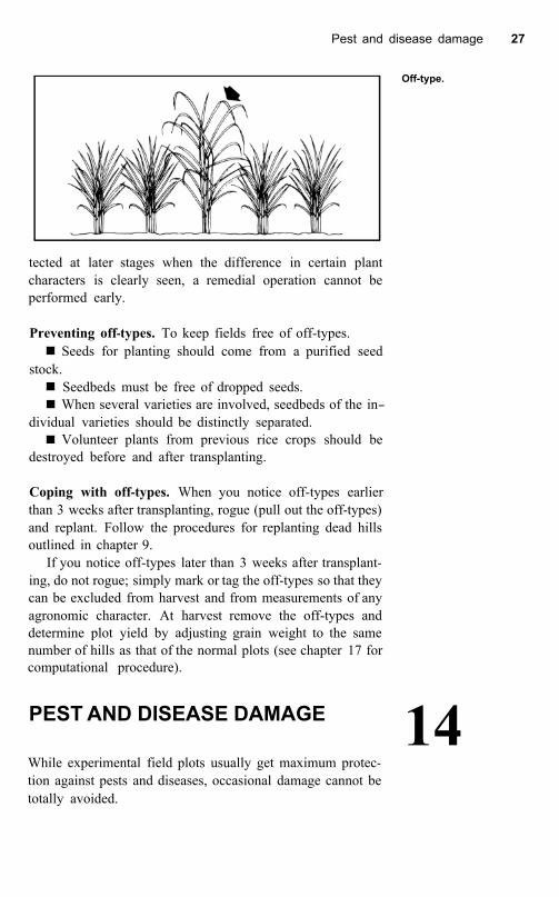
Pest and disease damage 27

Off-type.

tected at later stages when the difference in certain plant characters is clearly seen, a remedial operation cannot be performed early.

Preventing off-types. To keep fields free of off-types.

stock. Seeds for planting should come from a purified seed

Seedbeds must be free of dropped seeds. When several varieties are involved, seedbeds of the in-

dividual varieties should be distinctly separated.

destroyed before and after transplanting.

Coping with off-types. When you notice off-types earlier than 3 weeks after transplanting, rogue (pull out the off-types) and replant. Follow the procedures for replanting dead hills outlined in chapter 9.

If you notice off-types later than 3 weeks after transplant- ing, do not rogue; simply mark or tag the off-types so that they can be excluded from harvest and from measurements of any agronomic character. At harvest remove the off-types and determine plot yield by adjusting grain weight to the same number of hills as that of the normal plots (see chapter 17 for computational procedure).

Volunteer plants from previous rice crops should be

PEST AND DISEASE DAMAGE 14 While experimental field plots usually get maximum protec- tion against pests and diseases, occasional damage cannot be totally avoided.

28 Field technique

Seedlings near the edge of the seedbed tend to be larger than the rest.

Effect on experiment. Damage from pests and diseases usually occurs in spots, resulting in an increase in variation both among plots and within plots and, consequently, in experimental error. Moreover, the nonuniformity of the inci- dence can greatly affect the treatment comparisons.

Minimizing effects of damage. When a plot is damaged, do not take samples from plants damaged by pests and diseases for measuring any agronomic character (unless your objective is to evaluate damage).

When incidence in each plot does not involve a large number of plants, say, when not more than 20 percent of the plants in any plot is damaged, exclude damaged plants from the harvest of each plot. Later, convert the grain weight of each plot based on the number of hills in the normal plots (see chapter 17).

When only a few plots are heavily damaged, do not collect samples from these plots. They should be treated as “missing data” when the data are analyzed.

When damage is moderate to heavy, quite nonuniform from plot to plot, and measurable, harvest all plants in each plot in the usual manner. Collect data on pest and disease incidence for every plot. Use covariance analysis with the data on the incidences as covariates.

15 MINOR SOURCES OF VARIATION

Minor sources of variation should be controlled if you want a high degree of precision and if you can afford the cost.

Minor sources of variation 29

Dung from carabaos used during land preparation can increase soil hetero-

fertility. geneity in a field with low

Application of fertilizer. Variability is generally higher in fertilized fields than in unfertilized fields primarily because of nonuniform application of fertilizer. Several things to keep in mind:

Do not apply fertilizer to compensate for areas of the field that have seemingly poor fertility.

Fertillizer applied to a small plot tends to concentrate in the center of the plot because operators generally try not to spill the fertilizer outside the area specified.

When fertilizer is to be applied to a large field, the field can first be divided into smaller sections and the amount of fertilizer to be applied can be computed for each subsection separately. This results in more uniform application.

Choice of seedlings. Seedlings raised in any type of seedbed, generally vary in vigor. Seedlings located along the perimeter are usually bigger than those in the center. Choosing uniform seedlings for transplanting can increase the homogeneity of plants in the field. To ensure sufficient seedlings, raise more seedlings than you need.

Carabao dung. Carabao (water buffalo) dung causes addi- tional soil heterogeneity. In fields with low fertility, it usually results in a circular spot of very vigorous plants. When carabaos are used to prepare the land, dung should be removed from the experimental area.

32 Field technique

16 PLOT SAMPLING

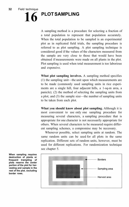
A sampling method is a procedure for selecting a fraction of a total population to represent that population accurately. When the total population to be sampled is an experimental plot as in replicated field trials, the sampling procedure is referred to as plot sampling. A plot sampling technique is considered good if the values of the characters measured from the sample are very close to those that would have been obtained if measurements were made on all plants in the plot. Plot sampling is used when total measurement is too laborious and expensive.

What plot sampling involves. A sampling method specifies (1) the sampling unit—the unit upon which measurements are to be made (commonly used sampling units in rice experi- ments are a single hill, four adjacent hills, a 1-sq-m area, a panicle); (2) the method of selecting the sampling units from a plot; and (3) the sample size—the number of sampling units to be taken from each plot.

What you should know about plot sampling. Although it is most convenient to use only one sampling procedure for measuring several characters, a sampling procedure that is appropriate for one character is not necessarily appropriate for others. When several characters to be measured require differ- ent sampling schemes, a compromise may be necessary.

Whenever possible, select sampling units at random. The same random units can be used for all plots in the same replication. Different sets of random units, however, must be used for different replications. For randomization technique see chapter 5.

When sampling requires destruction of plants or frequent trampling of plots reserve the center portion of the plot for har- vesting and sample in the rest of the plot, excluding border rows.

Plot sampling 33

When your sampling procedure requires the destruction of sample plants and frequent trampling of the plots, you may wish to separate the sample area from the rest of the plot. You can do this provided that the two areas are uniform and that randomization is still used in the sampling area. A common practice is to leave an area in the center of the plot for harvesting and use the surrounding areas for sampling.

For measuring the same character, say, height, at different growth stages, use the same sample plants at all stages of observation. If sampling is very frequent, change one-third (or one-fourth) of the samples at each stage of measurement to avoid possible effects from frequent handling of the sample plants. For example, in measuring plant height using eight sample hills per plot, the randomization at the first stage of observation may give the following positions of sample hills:

For the second stage of observation, retain six of the first eight sample hills and apply randomization technique to select two additional hills. The set of eight sample hills for the second stage of observation may be:

Hills B and H are the two newly selected hills.

34 Field technique

For suggested sampling unit and sample size for a particu- lar character, see chapters 17 to 22.

17 MEASURING GRAIN YIELDS

Grain yield refers to the weight of cleaned and dried grains harvested from a unit area. For rice, grain yield is usually expressed either in kilograms per hectare (kg/ha) or in metric tons per hectare (t/ha) at 14 percent moisture.

How to measure grain yield. After discarding border areas on all four sides of a plot (see chapter 7 for appropriate size of border areas), harvest as large an area as possible. For reliable results, the harvested area must not be less than 5 sq m per plot.

Thresh, clean, dry, and weigh all grains harvested from each plot separately.

Immediately after the grain from a plot is weighed, deter- mine its moisture content. Adjust grain weight to 14 percent moisture using the formula:

Adjusted grain weight = A × W

where A is the adjustment coefficient and W the weight of the harvested grains. The coefficient A can be read directly from Appendix Table 2 or computed:

100 - M A= 86

where M is the moisture content (percent) of the grains.

Handling missing hills and off-types. When one or more hills are missing, exclude from harvest all hills immediately adjacent to the missing hills (see chapter 8). When off-types are present, remove all of them from the harvest (see chapter 13). If the reduction in the number of hills harvested due to the presence of either missing hills or off-types is not more than 20 percent,

W n Grain yield/plot = × N

Measuring plant height and tiller number 35

where W is the weight of grains from harvested hills, n the number of harvested hills, and N the total number of hills in normal plots.

Do not harvest any plot in which the number of hills has been reduced by more than 20 percent. Treat such a plot as “missing data” when the data is analyzed.

Handling damage from pests and diseases. Sometimes factors you cannot control cause damage but have nothing to do with the treatments, as when plants are damaged by rats. When that occurs one approach is to exclude all damaged plants from the harvest and adjust grain weight of each plot based on the number of hills in the normal plots (see above formula), provided that the reduction of the number of hills in the plot is not more than 20 percent. Another approach is to measure the damage in each plot before harvesting all of each plot including damaged plants (see chapter 14). Apply covari- ance technique with the measure of damage as covariate.

When in doubt, consult a statistician.

When plants are destroyed in previous sampling. Make sure that the harvest area does not include plants adjacent to areas left empty from sampling for characters whose measure- ment involved destruction of plants at early growth stages.

MEASURING PLANT HEIGHT AND TILLER NUMBER 18 For seedlings or juvenile plants, plant height is the distance from ground level to the tip of the tallest leaf. For mature plants, it is the distance from ground level to the tip of the tallest panicle. Tiller number is the number of tillers per unit area or the number of tillers per plant when single-plant hills have been used. At harvest, tillers can be separated into productive and unproductive tillers.

Sampling. For plant height measurement, a single-hill sam- pling unit is optimum; for tiller count, a two-hill x two-hill sampling unit is optimum (Table 12). Since the two characters are usually measured at the same time, a two-hill x two-hill

36 Field technique

Table 12. Comparable variance, expressed as percentage of the mean, among sampling units of different sizes and shapes for measuring plant height and tiller number, under different fertilizer treat- ments.

Coefficient of variation (%)

Sampling unit (hill × hill)

Plant ht Tiller no.

0 kg/ha N 120 kg/ha N 0 kg/ha N 120 kg/ha N

1 ´ 1 4.4 3.1 33.6 31.8 1 ´ 2 4.9 3.4 33.4 31.4 1 ´ 3 4.8 3.7 30.3 31.2 1 ´ 4 5.6 3.8 28.3 30.1 2 ´ 2 5.6 3.8 26.2 29.5

sampling unit should be used. Count tillers on all four hills of each unit but measure plant height on only one hill per unit:

For plant height, the coefficient of sampling variation is slightly higher at early growth stages, but the difference is not appreciable. For tiller number, the coefficient of sampling variation does not vary with the growth stage (Table 13). Thus, the same sample size can be used at all growth stages.

Fertilizer application causes a small increase in the coeffi- cient of sampling variation of tiller number but not in that of plant height. Thus, to obtain the same degree of precision, a slightly larger sample size may be required for tiller count in fertilized plots than in unfertilized plots.

Sample size, or the number of two-hill x two-hill sampling units to be taken per plot, for varying degrees of precision desired can be determined from Table 14. Usually three two- hill x two-hill sampling units per plot (giving a total of 12 hills for tiller count and three hills for plant height) are sufficient.

Measuring plant height and tiller number 37

Table 13. Coefficients of variation among two-hill × two-hill sampling units for plant height and tiller number, under different

Coefficient of variation (%) Growth stage

transplanting) (days after Plant ht Tiller no

0 kg ha N 120 kg/ha N 0 kg/ha N 120 kg/ha N fertilizer treatments,

30 66 56 10.1 14.0 44 68 49 10.3 10.6 58 46 50 10.2 11.1

Harvest 49 42 10.8 11.8

Standard error (%) Sample size

Plant ht Tiller no

2

4 3

6 5

7 8

3.1 2.5 2.2 2.0 1.8 1.6 1.5

8.7

6.2 7.1

5.5 5.0 4.7 4.4

a Plant height is measured from only one hill out of each two-hill x two-hill sampling unit selected, while tiller count is made on all four hills per unit. b No. of two-hiII x two hill sampling units per plot

Table 14. Estimated stan- dard error of a plot mean for the measurement of plant height and tiller number for different sample sizes based on two-hill × two-hill sampling units a .

When measurements are to he made at various growth stages to examine the growth pattern, use the same sample plants for all stages. That is, there is no need to select new sampling units at each growth stage. If sampling is very frequent, change a fraction of the samples at each growth stage to avoid possible effects from frequent handling of the sample

Measurements of tiller number and especially of plant height can be greatly affected by observers. Try to avoid changing observers from plot to plot within a block. If you must change observers, change them from block to block (see chapter 4).

plants (see chapter 16).

MEASURING YIELD COMPONENTS 19 Some important yield components of rice are panicle num- ber— the number, at maturity, of fully exserted and grain- bearing panicles per plant or per unit area; number of filled grains per panicle— the average number of fully developed grains per panicle; percentage of unfilled grains— the propor- tion of poorly developed or totally undeveloped grains: grain

38 Field technique

Table 15. Estimated stan- dard error of a plot mean Standard error (%) for measuring yield com- ponents for different Sample size a No. of No. of filled Percentage 100-grain

two-hill × two-hill sampling sample sizes based on

unit.

panicles grains per unfilled wt panicle grains

2 8.7 4.3 10.1 3

1.7 7.1

4 3.6 8.2

6.2 1.4

3.1 7.1 1.2 5 5.5 2.8 6 5.0 2.5

1.1

7 4.7 1.0

2.3 5.4 0.9 8 4.4 2.2 5.0 0.9

6.4 5.8

a No. of two-hill × two-hill sampling units per plot.

weight — the weight of fully developed grains, commonly reported on the basis of 100 grains or 1,000 grains.

How to measure yield components. First, select at random n two-hill × two-hill sampling units from the test area (exclud- ing borders) of each plot. These sample hills must not be hills that were replanted or that are adjacent to a missing hill. Table 15 shows number of sampling units, n, to be taken for a specific degree of precision for each character. Usually, n = 3 (12 hills per plot) gives an adequate level of precision for most commonly measured yield components.

Second, count the total number of panicles ( P ) from all sample hills.

Third, from each sample hill, separate the center or middle panicle (based on height of the individual tillers) from the rest of the panicles.

Fourth, thresh and bulk the grains from the center panicles from all sample hills and separate the filled grains from the unfilled grains. To separate unfilled grains from filled grains, use a seed separator, the salt-water (sp gr 1.06) method, or the manual method. Count the filled grains ( f ) and the unfilled grains ( u ) and weigh the filled grains ( w ).

Fifth, thresh the grains from the rest of the panicles of all sample hills and separate unfilled grains from the filled grains. Then count the unfilled grains ( U ) and weigh the filled grains ( W ).

Sixth, compute the number of panicles per hill, number of filled grains per panicle, percentage of unfilled grains, and 100-grain weight:

Measuring leaf area index 39

P No. of panicles/hill = 4 n

f W + w No. of filled grains/panicle = × w P

Percentage of unfilled grains = × 100 U + u f ( W + w )/ W + U + u

100-grain wt = × 100 w f

Pointers. Weigh the filled grains in the fourth and fifth steps simultaneously to ensure that the grains of the two parts have a similar moisture content.

If you are determining yield components to compare computed yield with measured yield, in addition to obtaining the weight of filled grains in the fifth step, determine the percentage of moisture content of the filled grains ( M ). Then at 14 percent moisture

100 - M w 100 grain wt = × × 100 86 f

When a seed counter is available, you can count filled grains of all sample hills without having to take sub-samples of middle panicles, as was done in the third and fourth steps.

MEASURING LEAF AREA INDEX 20 The leaf area index (LAI) is the area of the leaf surface per unit area of land surface. Methods of measuring LAI are given for two conditions, one in which leaves are not removed from plants, and another in which leaves are removed.

Measuring LAI with leaves not removed from plants. Select at random n hills from each plot, making sure that each hill is surrounded by living hills. The values of n for any specific degree of precision are given in Table 16. In general. n = 10 is sufficient.

40 Field technique

Table 16. Estimated stan- dard error of a plot mean (not including measure- Sample Size a

ment error) for measuring leaf area index for varying sample size.

Standard error (%)

Unfertilized Fertilized

2 20.2 30.0 3 16.4 24.5 4 14.2 5

21.2

6 12.7 19.0 11.6

7 17.3

10.8 16.1 8 9

10.1 9.5

15.0 14.2

10 12

9.0 13.4 8.2 12.3

14 7.6 11.4

a No. of hills per plot. To take care of a higher measurement error when leaves are not removed a slightly larger sample size is required.

Count the tillers for each sample hill in each plot. Measure the length and maximum width of each leaf on the

middle tiller and compute the area of each leaf based on the length-width method:

Leaf area = K × l × w

where K is the “adjustment factor.” l is the length, and w is the width. The value of K varies with the shape of the leaf which in turn is affectedby the variety, nutritional status, andgrowth stage of the leaf. Under most conditions, however, the value 0.75 can be used for all stages of growth except the seedling stage and maturity for which the value 0.67 should be used.

Compute the leaf area per hill and leaf area index:

Leaf area hill = total leaf area of middle tiller × total number of tillers

Sum of leaf area/hill of n sample hills (sq cm)

area of land covered by n hills (sq cm) LAI =

Measuring LAI with leaves removed from plants. Select at random n hills from each plot, making sure that the hills are surrounded by living hills. The values of n for any specific degree of precision are given in Table 16. In general, n = 8 is sufficient.

For each plot remove the sample hills from the soil. From each sample hill, separate the middle tiller from the

rest of the tillers. Remove all green leaves from the selected

Measuring stem borer incidence 41

tiller. Make sure the leaves do not dry and curl before their leaf areas are measured. To avoid drying and curling, place the sample leaves in a test tube containing a small amount of water. Measure the area of the leaves. With an automatic area meter. you can read all leaves from each sample tiller together. With the length-width method, however, you should obtain the area for each leaf separately. Dry the leaves and weigh.

Remove leaves from the rest of the tillers in the sample hills and obtain their dry weight.

Compute leaf area per hill and leaf area index:

Leaf area/hill = aW w

Sum of leaf area/hill of n sample hills (sq cm) area of land covered by n hills (sq cm)

LAI =

where a is the total area of sample tiller, w the dry weight of leaves from sample tiller, and W the dry weight of all leaves in the hill (including those from the sample tiller).

MEASURING STEM BORER INCIDENCE 21 Stem borer incidence is generally determined from the pres- ence in the plot of dead hearts or white heads or both. Dead hearts are young tillers that turn brown and die before produc- ing heads. They indicate borer damage during the vegetative phase of the plant. White heads are culms with whitish panicles that remain upright. Most grains in these panicles are empty. The incidence of either dead hearts or white heads is generally measured as a percentage.

Measuring incidence by complete enumeration on in- fested hills. Count the number of infested and uninfested tillers in all infested hills in a plot. Then select a sample of 10 uninfested hills and count the tillers.

Compute the percentage incidence ( P ) of the plot:

P = nx + ( N - n ) y

I × 100

42 Field technique

where I is the total number of infested tillers from all infested hills, x the average number of tillers per hill from all infested hills, y the average number of tillers per hill from 10 uninfested hills, n the total number of infested hills, and N the total number of hills (infested and uninfested) in a plot.

Measuring incidence by sampling infested hills. When resources are limited and complete enumeration of all infested hills in a plot is not feasible, make observations only on every other two rows in a plot. Count the number of infested and uninfested tillers in all infested hills from each two-row unit. Then select a sample of 10 uninfested hills and count the tillers.

Percentage incidence of the plot is computed as before with

NOTE: The above procedures can also be used for meas- N as the total number of hills in all the rows examined.

uring gall midge incidence.

22 SAMPLING IN BROADCAST RICE

The greatest difficulty in sampling in broadcast rice plots lies in the identification of sampling units. In transplanted rice, the sampling unit used is based on hills which is not applicable to broadcast rice. In broadcast rice, the sampling unit must be identified in terms of area. But demarcating sampling areas for measuring various rice characters is an additional problem.

The nonuniform plant density in broadcast rice plots also causes higher variability than in transplanted rice. Thus, for most characters the sample size in broadcast rice should be larger than in transplanted rice.

How to sample broadcast rice. For grain yield in a broadcast plot, just before seeding outline the desired harvest area in the center of the plot with four small stakes connected with string. The string should be tied flush with the soil to avoid any effect on the seeding operation. Thus the string should be durable enough to withstand being covered with mud for the entire crop season. At maturity, harvest all plants in the demarcated area of each plot.

For other plant characters, construct rectangular wire frames, each 50 × 30 sq cm. Place three to four frames at random in

Sampling for protein determination 43

Wire frame tor sampling agronomic characters,

cast rice plots. other than yield, in broad-

each plot just before seeding. Various characters, such as tiller count and plant height, can be measured from plants within these units. If measurements are to be made at early growth stages, place these frames at random just outside the harvest area to prevent trampling of the harvest area.

SAMPLING FOR PROTEIN DETERMINATION 23 The measurement of protein content consists of the sampling procedure for selecting the sample grains and the chemical analysis of the selected grains. Since only a small sample is used in the chemical analysis, the sample must be properly selected.

Selection of sample grains. For protein analysis of individual plants, take the sample after all grains have been threshed and bulked. Do not sample panicles. For protein analysis of whole plots, take sample grains from the bulk harvest used for plot yield determination. Do not take hill samples.

Size of sampling unit. Use 100-grain (or 2-gram) samples and make two determinations per sample. When you only have a grinder with small capacity, 10-grain samples can be used. If you use a 10-grain sample, analyze at least two

44 Field technique

separate 10-grain samples, without duplicate analysis. Do not use a sample size smaller than 10 grains under any circum- stances.

REFERENCES

Cochran, W.G. 1963. Sampling techniques. 2nd ed. Wiley & Sons, Inc., New York. 413 p.

Cochran, W.G., and G.M. Cox. 1957. Experimental designs. 2nd ed. John Wiley & Sons. Inc.. New York. 611 p.

Gomez, K.A., and S.K. De Datta. 1972. Missing hills in rice experimental plots. Agron. J. 61: 163-164.

Gomez, K.A., and S.K. De Datta. 1971. Border effects in rice experimental plots. I. Unplanted borders. Exp. Agr. 7:87- 92.

Gomez, K.A., and R.C. Alicbusan. 1969. Estimation of opti- mum plot size from rice uniformity data. Philippine Agr. 52:586-601.

International Rice Research Institute. 1971. Annual report for 1970. Los Baños, Philippines. 265 p.

International Rice Research Institute. 1970. Annual report 1969. Los Baños, Philippine. 266 p.

International Rice Research Institute. 1969. Annual report 1968. Los Baños, Philippines. 402 p.

LeClerg, E.L., W.H. Leonard. and A.G. Clark. 1962. Field plot technique. 2nd ed. Burgess Publishing Co., Minnea- polis. 373 p.

Palaniswamy, K.M. 1971. Sampling in rice experimental plots. Unpublished MS. Thesis. Univ. Philippines [Col- lege, Laguna]. 84 p.

Sridodo. 1972. Sampling in broadcast rice plots. Unpublished M.S. Thesis. Univ. Philippines [College, Laguna]. 85 p.

Yoshida, S., D.A. Forno, J.H. Cock. and K.A. Gomez. 1972. Laboratory manual for physiological studies of rice. 2nd ed. International Rice Research Institute, Los Baños, Phil- ippines. 70 p.

46 Field technique

09724 14620

97310 56919

07585

25950 82973 60819 59041 74208

39412 48480 95318 72094 63158

19082

94252 15232

48392 72020

37950 09394 34800 36435 28187

13838 72201 63435 59038 62367

07896 71254

71433 54614 30176

79072 75014 37390 24524 26316

45836 61085

92103 10317 39764

83594 08087 57819 96957 48426

95430 85125

78209 17803

28040

85189

27364 16405

69516 38475

03642 50075 28749 16385 49753

73645 84146 77489

06359 18895

77387 59842 28055 75946 31824

79940 08423 45192 96983 45627

81686 62924 54331 19092 71248

87795 96754 75846 32751 20378

96937 41086

82592 19679

21251

95692 01753 39689 81060 43513

48477 12951

95781 51263 26939

69374 81497 59081 03615 79530

87497 11804 49512 90185 84279

09182 87729 62434 84948 47040

35495 39573 91570 85712 52265

97007 41489 62020 49218 58317

85861 35682 58437 83860 37983

23294 67151 74579 28350 16474

02520 41283

65205 16921

41749

52910 01787 32509 28587 82950

81953 42783 85069 52396 64531

37904 20863 72635

47649 84093

29735 24956 35408 72635 56496

73649 65584 20965 53072 05695

48192 51630 99154 06293 80494

67511 15498 47358 57179 76928

63973 42820 03542 11351 06073

61602 82741 94606 43090 62438

86801 97460 65924 12528 43789

23202 51631 87540 60905 79838

70473 17629

61594 82681 70570

06759

49180 94072

49731 53046

72182 14308

21814 86259 30618

56823 83641 20247 74573 79799

84518 78548 39603 85621 66428

87939 94911 32286 08062 50274

96086 43646 76797 32533 89096

62921 24283 54959

42496 79672

30980 51798

24367 12521

70565

93736 74978 38150 67404 45149

83603 09137 52491 66875 85437 92086 82611 70858 98412 74070

83615 09701 70799 59249

62748 39206 72537 46950

95420 41857

46309 28493 59649 16284 07564 70949 38352 94710 23973 25354

95208 49635

03994 25989 19468 34739

05342 54212 19520 92764

30210 23805 06461 06566 76846 77183 97764 53126 15703 05792

68417 21786 79392 65362 41659 31842 25074 06374 28705 45060

89681 50212 37385 37236 50437 13576

43498 95782 56032 42009

38385 69546 64276 78438 35310 31249 94672 07091 351 91 49368

58479 34924 29852 47271 31 724 60336

35496 87172 1581 7 12479

79608 01242 10817 53164

47872 1 461 4 80450 21082 071 43 73967

26453 93650 53045 78195 83468

63461 47920

47315 81736

69420

75091 83538 50969 36853 25238

01420 57052 19609 85397 21539

27837 21752 50369 37396 53376

09822

47269 19672

96484 50903

92829

72876 16496

49745 70452

47104 70757

42920 15101

30074

25101 42480 01968 52021 76830

07525 10724

18427 16074 23723

02148 91487 31 847 47615 18295

46857 75108

53290 84697 79762

82753 53920 15395 94969 48544

46768 43056 74372 52095 48207

24953 78967 16501 57039 54205

67510 93682 70904 59159 66578

27698 51396 02323

90804 14651

40749 72917

95390 46046 93436

87373 94156 15971 02350 41843

27035 72656 06725 61437 06909

30742 37190 36207 23721 32585

45703 31924 81736 30853 01935

47192 15040

26081 38405 20405

45362 29950 74151 18079 95920

42610 45692 68867 06096 91590

23817 84190 62972 23749 41465

62284 77975 95237 80128 12042

66273 85183 73432 38083 29425

61560 49341 07963

83489 76394

67562 80854 69326 24961 75375

Appendix Table 1. Random numbers.

Appendices 47

Appendix Table 1. Continued

57856 87037 57196 47916 15960 13036 84639 61684 96598 28043 25325 81767 20792 39823 06847 83825 12858 18689 41319 15959 38030 40810 85323 18076 02821 94728 96808 11072 06461 45073 88350 35246 15851 16129 57460

82197 35028 96295 95795 76553 50223 37215 47430 50260 03643 72259 71294 69176 21 753 25043 52002 84476 69512 95036 69095 96340 34718 11667 96345 60791 06387 54221 40422 23965 59598 09746 48646 47409 32406 80874

08261 71627 96865 75380 42735 19446 78478 67207 47166 44917 94177 31846 73872 92835

10289 93145 14456 32978 82587 64377 54270

62557 05584 27879 08081 01467 19691 39814 75622 83203 14951 46603 84176 17564 53965

51695 70743 68481 57937 62634 86727 69563 54839 69596 25201 56536 54517 86909 92927 75284 36241 59749 81958 44318 28067 67638

94649 33784 84691 48334 74667 48289 29629 64082 68375 30361 32627 38970 82481 94725

25261 28316 37178 82874 37083 73818 78758 21967 90859 05692 34023 09397 55027 39897 63749 41490 72232 71710 36489 15291 68579 63487 42869 24783 80895 78641 50359 20497 91729 08960 70364 14262 76861 06406 85253

38532 27650 6831 8 91 423 54574

93987 59854 12636 04856 9241 7

95723 14398 97643

3871 5 14020

56602 70051

69874 35242 20364

16572 74256 04653 32077 46545

523'6 57930 14851 83067 54648

91 493

51 498 13847

80651 96727

05695

48258 4791 6

36409 16902

31 424 58040 15653 79841 89248

14877

48391 15507

8721 4 23074

4 1320 25216 96592

29806 57594 59360 50925 67180 42352 41671 78178 44278 80631 82547 39787

29265 63051 07586 78418 48489 14837 03817 21850 39732 18603

61816 09628 31397 17607 57095 37190 47369 39657 45179 061 78 34352 52548 57125 24634 95394 35242 60595 61636 97294 56276 90734 84549 04236 02520 29057

64543 12870 17646 25542 91526 56272 10835 76054 67823 07381 46058 34375 29890 71563 82459 47286 27208 09898 04837 13967 52324 96537 99811 60503 44262

26201 88098 31019 36195 23032 48323 37857 99639 10700 98176 70998 02969 42103 01069 68736 46481 17365 84609 26357 60470 58280 41596 87712 97928 45494

42927 46635 09564 45334 63012 02159 21981 00649 40382 43087 78424 67282 46854 61980 10745 14924 45190 51808 30474 29771 80308 52685 95334 12428 50970

30186 48347 40780 48749 79489 39329 80057 67617 18501

34512 10243 47635 39823 63756 04478

07692 76527 80764 58341 07468 1921 9 89713 06381 61522 93251 43456 89176 74010 91548 79394

35681 07769 18230 12596 64807 23978

47869 66444 68728 80771 10453 87972 66538 65243 76009

29308 51729 10453 07827 28271 52075 72196 54648 36886 56930 34939 27641 61248 47276 76161

97096 48508 26484

83195 60186 78142 51482 81867 81783

91381 72319 83280 57490 80497 54272

18752 12856 09537 09058 42479 60463 97394 98513 29634 27174 71319 82016 05425 27931 84965

47154 40798 06217 58918 37965 32031 71846 98148 12839 30294 62698 47548 22102 18358 95938

91395 46359 52952 96863 72547 29368 37210 65765 82546 24974 55274 79587 70562 82081 64785

92648 74724 68292 34642 43428 39068 52765 23824 31235 35212 51863 00401 78356 72100 32949

47305 27136 19428 34506 53229 08383 73924 12717 25524 51573 82713 69487 47019 21993 43350

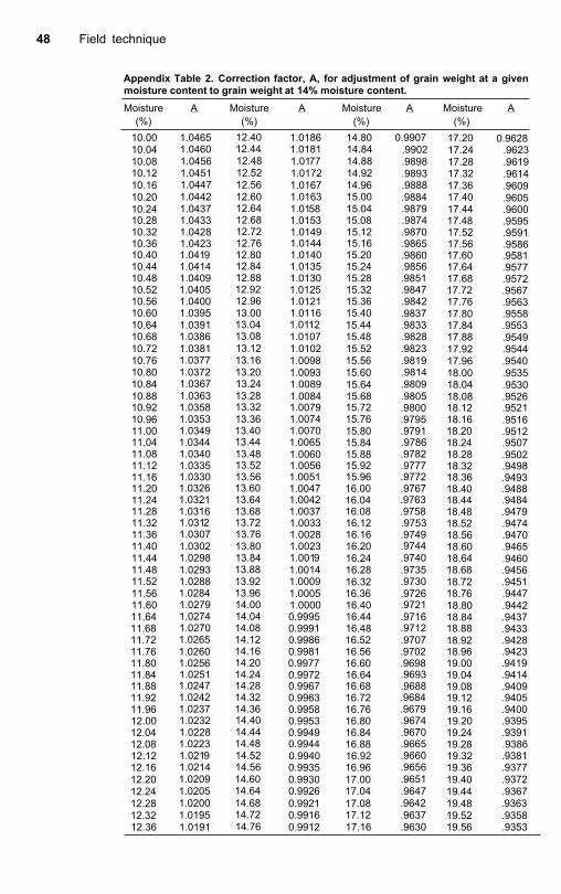
48 Field technique

Appendix Table 2. Correction factor, A, for adjustment of grain weight at a given moisture content to grain weight at 14% moisture content. Moisture A Moisture A Moisture A Moisture A

(%) (%) (%) (%) 10.00 10.04 10.08 10.12 10.16 10.20 10.24 10.28 10.32

10.40 10.36

10.44 10.48 10.52 10.56

10.64 10.60

10.68 10.72 10.76 10.80

10.88 10.84

10.92 10.96

11.04 11.00

11.08 11.12 11.16 11.20 11.24 11.28 11.32 11.36 11.40 11.44 11.48 11.52 11.56 11.60

11.68 11.64

11.72 11.76 11.80 11.84 11.88 11.92 11.96 12.00 12.04 12.08

12.16 12.12

12.20 12.24 12.28 12.32 12.36

1.0465 1.0460 1.0456 1.0451 1.0447 1.0442 1.0437 1.0433 1.0428

1.041 9 1.0423

1.0414 1.0409 1.0405 1.0400 1.0395 1.0391 1.0386 1.0381 1.0377 1.0372 1.0367 1.0363 1.0358 1.0353

1.0344 1.0349

1.0340 1.0335

1.0326 1.0330

1.0321 1.0316 1.031 2 1.0307 1.0302 1.0298 1.0293 1.0288 1.0284 1.0279 1.0274 1.0270 1.0265 1.0260 1.0256 1.0251 1.0247 1.0242 1.0237 1.0232

1.0223 1.0228

1.021 9 1.0214 1.0209 1.0205 1.0200 1.0195 1.0191

12.40 12.44 12.48

12.56 12.52

12.60 12.64 12.68 12.72

12.80 12.76

12.84 12.88 12.92 12.96

13.04 13.00

13.08 13.12 13.16 13.20

13.28 13.24

13.32 13.36 13.40 13.44 13.48 13.52

13.60 13.56

13.64 13.68 13.72 13.76 13.80 13.84 13.88 13.92 13.96 14.00

14.08 14.04

14.12 14.16 14.20 14.24 14.28 14.32 14.36 14.40

14.48 14.44

14.52 14.56 14.60 14.64 14.68 14.72 14.76

1.0186 1.0181 1.01 77

1.0167 1.0172

1.0163 1.01 58 1.0153 1.0149 1.0144 1.0140 1.0135 1.0130 1.0125 1.0121

1.01 12 1.0116

1.0107 1.0102 1.0098 1.0093 1.0089 1.0084 1.0079 1.0074

1.0065 1.0070

1.0060 1.0056 1.0051 1.0047 1.0042 1.0037 1.0033 1.0028 1.0023 1.001 9 1.0014 1.0009 1.0005

0.9995 1.0000

0.9991 0.9986 0.9981 0.9977 0.9972 0.9967 0.9963 0.9958 0.9953 0.9949 0.9944

0.9935 0.9940

0.9930 0.9926 0.9921 0.9916 0.9912

14.80 14.84 14.88

14.96 14.92

15.00 15.04 15.08 15.12

15.20 15.16

15.24 15.28 15.32 15.36

15.44 15.40

15.48 15.52 15.56 15.60 15.64 15.68 15.72 15.76 15.80 15.84 15.88 15.92

16.00 15.96

16.04 16.08 16.12 16.16 16.20 16.24 16.28 16.32 16.36 16.40 16.44 16.48 16.52 16.56 16.60 16.64 16.68 16.72 16.76 16.80 16.84 16.88

16.96 16.92

17.00 17.04 17.08 17.12 17.16

0.9907 17.20

.9898 17.28

.9902 17.24

.9893 17.32

.9888 17.36

.9884 17.40

.9879 17.44

.9870 17.52

.9874 17.48

.9865 17.56

.9860 17.60

.9851 17.68

.9856 17.64

.9847 17.72

.9842 17.76

.9837 17.80

.9833 17.84

.9823 17.92

.9828 17.88

.9819 17.96

.9814 18.00

.9809 18.04

.9805 18.08

.9800 18.12

.9795 18.16

.9791 18.20

.9786 18.24

.9782 18.28

.9777 18.32

.9772 18.36

.9767 18.40

.9763 18.44

.9758 18.48

.9749 18.56

.9753 18.52

.9744 18.60

.9740 18.64

.9735 18.68

.9730 18.72

.9726 18.76

.9721 18.80

.9716 18.84

.9712 18.88

.9702 18.96

.9707 18.92

.9698 19.00

.9693 19.04

.9684 19.12

.9688 19.08

.9679 19.16

.9674 19.20

.9670 19.24

.9665 19.28

.9660 19.32

.9656 19.36

.9651 19.40

.9647 19.44

.9642 19.48

.9637 19.52

.9630 19.56

0.9628 .9623 .9619

.9609

.9614

.9605

.9600

.9595

.9591

.9581

.9586

.9577

.9572

.9567

.9563

.9553

.9558

.9549

.9544

.9540

.9535

.9526

.9530

.9521

.9516

.9512

.9507

.9502

.9498

.9493

.9488

.9484

.9479

.9474

.9470

.9465

.9460

.9456

.9451

.9447

.9442

.9437

.9433

.9428

.9423

.9419

.9414

.9409

.9405

.9400

.9395

.9391

.9386

.9381

.9377

.9372

.9367

.9363

.9358

.9353