techniques for elliptic fluid-flow in prodlens(u) …
TRANSCRIPT

-A0-ft6g 4?1 ADAPTIVE GRID TECHNIQUES FOR ELLIPTIC FLUID-FLOW inPRODLENS(U) STANFORD, UNIV CR CENTER FOR LARGE SCALESCIENTIFIC CONPUTATION S C CARUSO ET AL. DEC 85
UN CL SSIFIED CLSSIC-85- NU±4- - 2- K-633F/ 24NML
3.6.
11111- I- 11111_L8.
1I111L2 11111J.4
V E O T, )N TJ T C AP
%A A.8 9 A <AQ,-7 96 3
CLaSSiC Project December 1985Manuscript CLaSSiC-85-10
Adaptive Grid Techniques for Elliptic
Fluid-Flow Problems
Ni
S.C. Caruso
J. H. Ferziger "TIC."LECTE
J. Oliger J 2-
Center for Large Scale Scientific ComputationBilding 160, Roon 313
CStanford University'IL Stanford, California 94305
AC.2
Apived lot puablic e lese
,
ADAPTIVE GRID TECHNIQUES FOR ELLIPTIC FLUID-FLOW PROBLEMS
by
S. C. Caruso, J. H. Ferziger and J. Oliger
Work done within the
Center for Large Scale Scientific Computing
(CLaSSiC)
Under support from
The Office of Naval Research
Grant N00014-82-K-0335
December 198
° I
--
pO.,
t.a
December 1985
A~ fi~,.g~ ~saAA~tL.L~t >2.'f-CVI;?. .... %.t..%. . ---. ,
L --... r -7 -
Acknowledgments
The authors thank Dr. Marsha Berger for providing assistance in
understanding her data structures and grid-generation subroutines. The
authors also thank Professor Abdel Zebib for supplying us with his
working version of the SIMPLER code.
The financial support for this project was provided by the Office
of Naval Research through the Center for Large-Scale Scientific Computa-
tion under contract N00014-82-K-0335. It is greatly appreciated.
Mrs. Ruth Korb has done an excellent job of editing and typing this
report. Her efforts are very much appreciated.
Accesion For
NTIS CRA&IDTIC TAB .
JuAlfc ito'
Dt _t; ibution
Avaiiabiiily Co es jDist
2..
i-ii:
A -1""
... ... .. .. . .. . . ... ..,': :::

Abstract
We describe, adaptive grid techniques for elliptic fluid-flow prob-
lems. The primary applications are to flows described by the steady,
incompressible laminar and Reynolds-averaged Navier-Stokes equations.
The method can be extended to other elliptic flows. The current version
of the adaptive method is designed for use on a single, uniform, rectan-
gular grid or unions of such grids. Other geometries could be handled
by means of commonly used mapping or composite grid techniques.
-Oumethod is an extension of a local refinement technique devel-
oped by Berger for systems of hyperbolic equations. Local refined grids
are overlaid on a coarser base grid. Recursive use of this technique
allows an arbitrary degree of grid refinement. In two dimensions, the
refined grid consists of uniform rectangles having arbitrary rotation.
Regions neeuing refinement are defined using local error estimates.
The base grid remains fixed, and refinements are added as needed.
This method contrasts with global refinement methods, in which a fixed
number of points on a single grid are iteratively redistributed
according to some criterion such as the local solution gradient,
curvature, etc.
-Two classes of elliptic flows are identified; they are character-
ized as having strong or weak viscous-inviscid interactions. Adaptive
solution strategies, active and passive, respectively, are developed for -S
each class.
The passive method is applied to linear problems in one and two
dimensions. In 2-D, the refined grids automatically aligr. with the
flow, thereby minimizing numerical diffusion. The adaptive method is 6
shown to be more efficient than using a uniform fine grid.
The SIMPLER method is used to solve the steady, laminar, incompres-
sible Navier-Stokes equations. Central differencing of the convective
terms is implemented with the defect-correction method to stabilize the
solution method for all cell Reynolds numbers. Smooth solutions are
calculated for cell Reynolds numbers as high as 150, indicating that the
commonly used restriction, ReAx < 2 is too severe. Uniform-grid
iv

calculations are performed for the laminar backstep flow. Patankar's
power-law scheme is shown to be less accurate than central differencing,
and only first-order accurate.
Richardson-estimated solution and truncation errors are compared to
accurate estimates of the same quantities for the backstep flow. The
solution error is well predicted. The truncation-error estimates are
less accurate, but they reliably indicate where grid refinement is
required.
Active-adaptive calculations of the backstep are made, using
boundary-aligned refinement. At Re - 100, the adaptive calculation
has comparable accuracy, but is six times faster than a uniform-grid
calculation; the advantage is greater at higher Reynolds numbers.
Adaptive calculations are also made at higher Reynolds numbers. The
calculations agree well with the experimental data and other calcu-
lations.
iV
............

Table of Contents
Page01Acknowledgments . . . . . . . . . . . . . . . . . . . . . . . . . iii n
List of Figures . . . . . . . . . . . . . . . . . . . . . . . . . viii
Nomenclature 0 . . . . . . . . . . . . . . . . . xii
Chapter
1.* INTRODUCTION . . . . . . . . . . . . . . . . . . . . . . . 1
1.2. Adaptive Grid Methods . . . . . . . . . . . . 21.2.1. Global Refinement Methods .. . . . . . . . 31.2.2. Local Refinement Methods . .. .. .. . . 10
2. REVIEW OF BERGER'S METHOD . . . . . . . . . . . . . . . . 17
2.1. Overview.. . . . . . . . . . . . . . . 172.2. Grid Description . ........ .* . . . 172.3. Adaptive Solution Procedure . . . . . . .. . 192.4. Error Estimation . .00 . . . . . . . . . . . 212.5. Refined-Grid Generation . . . . *.... . . . . 232.6. Boundary Values for Refined Grids .. . 242.7. Data Structures ooo . . . . . oo . . . . .. ... 26
3. STRATEGYFOR ELLIPTIC EQUATIONS o. . . ... .. ... 31
3.1. Overview o . . . . . . . . . o 31
3.2. Influence of Elliptic Equations on Adaptive Approach 313.3. Two Adaptive Strategies . . . ... 323.4. Passive Method . . . . . . . . . . . . .... . . 35
3.4.1. Strategy . . . . . . . . 0... . . . . . 35
3.4.2. Summary of Theoretical Results . .. .. . .36
3.5. Active Method . * . . . . . . 0. . 6 ... . . . 383.6. Solution on Overlapping Grids . .. .. .. .. . .42
3.7. Error Estimation. .. ....... . . . . 453.8. Initial Guesses and Boundary Values for Refined
r.Grids . .. .. .. .. .. .. . .. . . . . . . . 49
I.I
4. APPLICATION TO ONE-DIMENSIONAL BOUNDARY-VALUTE PROBLEMS .. 57
I,4.1. Introduction.......*.. . . . . . . . . . . 574.2. "umerical Method ..... . . . . .. .. .. . .58
4.3. Adaptive Procedure . .... . . . .. .. .. . .58
4.4. Numerical Results...... .. .. .. .. .. .. .. . 594.5. Conclusions........ ... . ... .. .. .. .. .. . 63
IF 5. APPLICATION TO A TWO-DIMENSIONAL, LINEAR, CONVECTION-DIFFUSION PROBLEM . . . . . . . . . . . . . . . . . . . . 75
5.1. Introduction .. ..................... 755.2. Numerical Method. .. ................. 765.3. Adaptive Procedure .. ........ . .. .. .... 775.4. Numerical Results .. ................. 795.5. Conclusions .. .................... 82
6. NUMERICAL SOLUTION OF THE NAVIER-STOKES EQUATIONS . . . . 87
6.1. Navier-Stokes Equations. ..... .................. .. 876.1.1. The Incompressible Navier-Stokes Equations 87
U vi

LJ
6.1.2. Reynolds-Averaged Equations ... ....... . 886.1.3. Eddy-Viscosity Models .. . . . . . . .. 896.1.4. Steady, 2-D Laminar Equations . ....... . 91
6.2. Staggered Grid . . .. . . . . . . . . . . . . . 92
6.3. Finite Differences . . . . . . . . . ....... 936.3.1. Pressure Difference . . . . . . . . . . . . 946.3.2. Diffusion Terms ... ......... . . .. . . 94
6.3.3. Convective Terms . . . . . . . . . . . . . . 96a. Central Differencing . . . . . . . .. 97b. Upwind Differencing . . . . . . . . . . 98c. Hybrid Differencing . . . . . . . . . . 99d. QUICK Differencing. . . . . . . . . . . 100
6.4. SIMPLER Solution Technique . . . . . . . . . . . . . 1016.4.1. Pressure Calculation . . . . . . . . . .. 1026.4.2. Momentum Calculation . . . . . . . . . . . . 1036.4.3. Velocity and Pressure Corrections . . . . . 104
6.4.4. Solution of Linear Systems . . . . . . . . . 1056.5. Implementation of Central Differencing for Reax > 2 1066.6. Numerical Conservation . . . . . . . . . . . . . . . 108
7. ADAPTIVE NAVIER-STOKES SOLVER . . . . . . . . . . . . . . 115
7.1. Summary of Adaptive Process . . . # . . . . . . . . 1157.2. Implementation of the Active Solution Method . . . 1167.3. Treatment of Boundary Conditions . . . . . . . . . . 118
7.3.1. Interpolation of Fine-Grid Boundary Con-ditions . . . . . . . . . .. 118
7.3.2. Modification of Coarse-Grid BoundaryConditions . . . . .... . . .... 119
7.3.3. Interpolation and Conservation for RotatedGrids . . . *. . . . . . . . . . . . . .. . 120
7.4. Error Estimation ..... . . . . . . . . . . . 122
8. APPLICATION TO THE LAMINAR BACKSTEP ..... . . . . 129
8.1. Description of the Problem ..... . . . . . . 129
8.1.1. Experiment of Armaly et al .. . . 1298.1.2. Computational Model .. ............ 130
8.2. Uniform Grid Calculations . . . . . . . . . . . . 1318.2.1. Velocity Profiles .......... . . 1328.2.2. Comparison of Convective Difference Schemes. 1338.2.3. Exact vs. Estimated Errors . . ....... 135
8.3. Preliminary Adaptive Calculations at Re 1 100 . . . 1378.3.1. Notation for Refined Grids. ......... 1388.3.2. Convergence of the Active Solution Method 1388.3.3. Iteration Strategy: Inner vs. Outer . . .. 139
8.3.4. Effect of Internal Fine-Grid BoundaryLocation ..................... . 140
8.4. Adaptive Performance Evaluation for Re 1 100 . . . 1418.5. Adaptive Results for 100 < Re < 600 .. ........ . 142
9. CONCLUSIONS AND RECOMMENDATIONS .... ............. . 179
REFERENCES .... ........... .................. 183
Appendix A QUANTIFICATION OF THE STRENGTH OF THE VISCOUS-INV[SCID INTERACTION ...... ................ . 189
vii
-4 -4 ~4* ***~~~.*.- -MEN"

List of Figures
Figure Page
2.1. Overlapping, component grids . . . o . * . .. .. .. 28
2.2. Example of overlaid grid structure . o . .o. . . . . o 28
2.3. Time integration on three-level grid structure . . . . 29
2.4. Richardson extrapolation for time-explicit method . . 29
2.5. Tree data structure . . . . o . . . . . .. . .. . . . 30
3.1. Developing boundary layer in a plane channel ... ....... 52
3.2. Quantification of boundary-layer coupling o . . . . . . 52
3.3. Example of newly refined regions . ... . .. .. . 53
3.4. Notation for active solution on two-level grid system . o . 53
3.5. Difference stencils and coarse-grid correction terms o . . 54
3.6. Notation for solution on overlapping grids ......... 54
3.7. Local cell coordinates for bilinear interpolation . . . 55
4.1. Example 1-D grid structures . . . . . . . . . .6
4.2(a). Simple boundary layer: base grid solution . . . . .. . 66
4.2(b). Simple boundary layer: solution on second-level grid . o . 67
4 .2(c). Simple boundary layer: solution on third-level grid . . o 68
4.2(d). Simple boundary layer: complete adapted solution . . . 69
4 .2(e). Simple boundary layer: central difference solution on base
grid . . . . ....................... 70
4.3. Adapted solution for two-boundary-layer problem ...... 71
4.4. Adapted solution for internal boundary-layer problem o o . . 72
4.5. Adapted solution for boundary layer with non-constant outersolution .. . ... ............................ 73
4.6. Adapted solution for problem with a turning point and a
boundary layer . ...................... 74
5.1. Schematic of linear convection-diffusion problem ...... 83
viii

- -- -- ~ ' ~ &~P ~~ ~ .Fj .... r~ wiV wP . V V~ 7 k _ __2__ __0 _-M -p . - I - -
5.2(a). Initial refinement region . . . . . . . . . . . . . . 84
5.2(b). First-level refined .:ds . . . . . . .. .. .. .. . .84
5.2(c). First-level refinement region . . . . . . . . . . . ... 85
5.2Cd). Resulting refined grids . . . . .. .. .. .. .. . .. 85
5.3. Adaptive vs. uniform grid performance . .. .. .. .. .. 86
6.1. Staggered grid geometry .. .. .. .. .. .. .. ... 111
6.2. Centered differences on staggered and nonstaggered grids .112
6.3. Finite volume for u .................... 113
*6.4. Difference stencil for boundary cells ............ 113
6.5. Finite volume for p . . . .. .. .. .. .. .. .. . .114
6.6. Line-by-line solution method . . . .. .. .. .. .. . .114
7.1. Boundary-aligned refined-grid geometry. ........... 124
7.2. Notation for active solution on two-level, 2-D grid system . 125
7.3. Conservative coarse-to-fine grid interpolation. ....... 126
7.4. Interpolation for rotated grids . . . . . . . . . . . . .. 127
8.1(a). Backatep geometry. .................... 150
8.1(b). Base grid for backstep. .......... . . . . . . .. 150
8.2. u(x,y) for Re - 100. ................... 151
8.3. v(x,y) for Re - 100 .......... .. .. .. .... 152
8.4(a). u(x,y - 0.0625) for Re - 100..............153
8.4(b). u(x,y - 0.5625) for Re - 100.............. 153
8.4(c). u(x,y - 0.8125) for Re -100..............154
8.4(d). u(x,y - 1.0625) for Re - 100..............154
8 .4(e). u(x,y -1.5625) for Re - 100 .............. 155
8.4(f). u(x,y - 1.8125) for Re - 100..............155
8.5(a). u(x -I.0,y) for Re -100 . .. .. .. .. .. .. . .156
*8.5(b). u(x - 4.0,y) for Re -100. ............... 156
ix

8.5(c). U(x- 6.0,y) for Re- 100 . . . . . . . . . . . . . 157.
8.5(d). u(x - 12.0,y) for Re -100 . . . . . .. .. .. .. 157
8.6(a). v(x,y - 0.25) for Re -100 . . . . . . . . . . . . .. 158
8.6(b). v(x,y - 0.75) for R~e -100 . . . . . . . . . . . . .. 158
8.6(c). v(x,y - 1.0) for Re 100 . . . . . . . . . . . . . .. 159
8.6(d). v(x,y - 1.25) for Re 100 . . . . . . . . . . . . .. 159
8.6(e). v(x,y -1.75) for Re 100 . . . . . .. .. .. .. .160
8.7(a). v(x -l.0,y) for Re - 100 . . . . . .. .. .. .. .161
8.7(b). v(x - 4.0,y) for Re - 100 . . . . . .. .. .. ... 161
8.7(c). v(x - 6.0,y) for Re - 100 . . . . . . . . . . .. . 16.2
8.7(d). v(x - 12.0,y) for Re -100 . . . . . . . . . . . .. .. 162
8.8. Comparison of difference schemes; u(x,Ax,y -0.8125) lk31.3
8.9. Comparison of difference schemes; v(x,Ax,y - 1.25)......164
8.10. Comparison of difference schemes; error vs. Ax .. 165
8.11. Solution error in u for Re 100 . . . . . . . . .. . 16.6
8.12. Solution error in v for Re =100 . . . . . .. .. .. .16.
8.13. Truncation error in u for Re - 100 . . . . . . . . . .. 17.0
8.14. Truncation error in v for Re - 100 . .. .. .. .. . 172
8.15. Rotated refined rectangles for backstep . .. .. .. .. .174
8.16. Notation for refined grids. ................ 174
8.17. Convergence of active method on two-level grid system . .. 17.5
8.18(a). Effect of internal boundary location; xL 4 4.. .... 176*
8.18(b). Effect of internal boundary location; XL 6 6... ... 176.
8.19. Reattachment length vs. Reynolds number........ .... 177
x

List of Tables
Table P age
4.1. Refined Grids for Example 1 . . . . . . . . .o. .. .. .. 64
8.1. Parameters for Uniform-Grid Calculations.... ........ 145
8.2. Uniform Grid Error .o . . . . . . ... ..... . . . . 146
8.3. Inner Iteration Strategy . . . . . .. o. o.. .. . ... 147
8.4. Adaptive vs. Uniform Grid Performance for Re -100 o 148
8.5. Summary of Adaptive Backstep Calculations.o...........149
Xi

Nomenclature
ajj Elements of matrix A.
Au , Av Proportionality variables in Eq. (6.4.6).
c Constant in Eqs. (6.1.8)-(6.1.10).
cel, C2 Constants in Eq. (6.1.12).
erms rms solution error.
e(h,x) Solution error.
e(h,x) Solution error estimate.
Gk Represents all grids at k-th refinement level.
Gkj J-th component of Gk.
h Mesh size; step height.
H Mesh size.
k Time step; turbulent kinetic energy.
K Ratio of mesh size to time step; sensitivity parameter inEq. (A.8-9).
L Differential operator; length scale.
Lh Difference operator.
LP, p-th order difference operator for x-momentum equationwith mesh size H.
LP,H p-th order difference operator for y-momentum equationwith mesh size H.
L - I Green's function.
Lh I Inverse of Lh .h h
m Mass flux.
M Matrix containing second moments of a set of flaggedpoints.
MX x-derivative of pressure.
MY y-derivative of pressure.
n Outward unit-normal vector.
xii
LI

N Number of grid points.
NX Ny Number of mesh lengths in x and y directions, respec-tively.
p Pressure.
p' Pressure correction.
Pe Peclet number.
Q Volumetric flow rate.
Difference operator.
R Refinement ratio.
Re Reynolds number.
Re~x Cell Re,'nolds number.
Reeff Effective Reynolds number.
S Source term for scalar equation.
S Source term for scalar pressure equation.p
t Time.
u Velocity vector.
u x-component of velocity.
um Maximum inlet velocity.
v y-component of velocity.
u , v Intermediate velocities calculated from Eq. (6.4.3).
uh, vh x- and y-components of velocity on a grid with mesh sizeh.
V Velocity scale.
Vo Velocity outside of boundary layer.
x Spatial coordinate.
XLk x-location of downstream boundary of 1k.
KR Reattachment length.
Xm' Ym Mean values of a set of x,y pairs.
xl, x2 Left and right grid boundaries.
xiii
7 . ~ .

y Spatial coordinate.
Yo Location of discontinuity at upstream boundary in Eq.
(5.4.1).
Y1 9 Y2 Left and right boundary values.
w I w2 Weighting functions in Eqs. (6.6.4).J w'
Subscripts
e East face of control volume.
h Fine grid quantity.
H Coarse grid quantity.
i Row index.
j Column index.
k Refinement level.
L, R Left and right boundary locations.
n North face of control volume.
s South face of control volume.
w West face of control volume.
Superscripts
m, n Iteration index
p, q Order of accuracy.
x x-momentum equation.
y y-momentum equation.
Fluctuating quantity.
Greek Symbols
a , ay Masking arrays, Eq. (7.2.1).
6 Boundary-layer thickness.
6 Displacement thickness.
6max Maximum allowed estimated solution error.
E Diffusion coefficient (perturbation parameter); turbulentdissipation.
xiv
:" x2!
,x ' 2 '.'; ;<' '.;:'.2 " .'.: .: '.: '_-' .: .- _' , -/ . ;-.,. ." - . . -.' . '.- - -'-T.

rk Boundary of Gk .
Yk Internal fine-grid boundary of Gk.
Qk Domain of Gk .
T(h,x) Truncation error.
*(h,x) Truncation error estimate.
Tmax Maximum allowed truncation error.
"" Relaxation factor in Eqs. (6.4.10)-(6.4.11).
*Passive scalar.
e Exact solution to Eq. (5.2.1).
vk, ae Constants in Eqs. (6.1.11)-(6.1.12).
, Angle of rotation.
, ii Rotated coordinates.
p Fluid density.
v Kinematic viscosity.
vT Eddy (turbulent) viscosity.
eff Effective viscosity.
6/6 x Generalized difference operator for first derivative.6+/64 Backward difference operator for first derivative.
6a Forward difference operator for first derivative.
6 , 62/6x2 Difference operators for second derivative.
AOsz Stopping criterion for Schwarz iterations.
AOGS Stopping criterion for Gauss-Seidel iterations.
V 2 Laplacian operator.
Gradient operator.
&x Mesh size in x-direction.
AY Mesh size in y-direction.
Other Symbols
(-) Average value.
xv

Chapter 1
INTRODUCTION
1.1 Motivation
Computational fluid dynamics (CFD) is playing an increasingly
important role in the design and analysis of energy-conversion and
transportation systems, due to the development of solution algorithms
that are efficient and accurate and to the rapid advances made in compu-
ter technology. However, there is always a need for more efficient
algorithms. Design studies require repeated calculations of a given
problem in order to search a parameter space, and engineers are contin-
ually tackling more complex and hence computationally more challenging
problems.
Many of the flows encountered in these systems are governed by
elliptic partial differential equations whose solutions may exhibit fine
structure within small regions of the computational domain. Many tradi-
tional solution techniques require a fine mesh covering the complete
domain in order to resolve these fine local details. This method is
inefficient, since the fine mesh is not needed in parts of the flow
where the solution has a moderate variation. In some cases, this inef-
ficiency can be tolerated; in others, it can be prohibitively expensive.
A lack of resolution is also a hindrance to the development of tur-
bulent closure models. Kline et al. (1982) point out that it is diffi-
cult to distinguish the numerical errors from modeling errors, and they
call out for procedures that can guarantee a prescribed level of numeri-
cal accuracy.
Adaptive grids can simplify solutions to problems that need refine-
ment only in small, localized regions of the domain. In these methods,
the mesh is changed or adapted as the solution develops. The mesh is
adjusted or refined to accurately resolve fine structures as they appear
in the numerical solution. The result is a nonuniform distribution of
grid points that provides the desired level of accuracy at much lower
cost than a uniform fine grid.

; OT ; 0
In the remainder of Chapter 1, we review existing adaptive grid
methods. We then review the technique developed by Berger (1982) for
hyperbolic equations. We have applied this approach to elliptic prob-
lems. Chapter 2 describes Berger's method in some detail. In Chapter 3
we present the strategy for applying Berger's method and the issues par-
ticular to elliptic eauations. Chapter 4 describes the application of
our method to linear, two-point, boundary-value problems. In Chapter 5,
results and a performance evaluation are given for a two-dimensional,
linear, convection-diffusion problem.
We discuss the basic solution technique and pertinent issues for
the Navier-Stokes equations in Chapter 6. Chapter 7 describes the fea-
tures of our adantive Navier-Stokes solver. In Chapter 8, we present
-" numerical results, including a performance evaluation for the method
" applied to the laminar, backward-facing-step problem. We draw conclu-
sions and make recommendations for further improvements of the method in
Chapter 9.
1.2 Adaptive Grid Methods
The development of adaptive grids is probably the most important
area of research in grid generation at present (Thompson, 1984). Many
approaches have been developed for a variety of differential equations
. and applications. These include steady and unsteady problems, hyper-
bolic, parabolic, elliptic, mixed equations, etc. It would be difficult
to make a classification for all adaptive grid methods, but most methods
can be fit into two different categories.
The first category is the "moving mesh" technique. Here, the total
number of grid points is fixed, and the mesh is adjusted by moving the
- points away from regions that have small solution variation and towards
regions having large variation. The method of moving the points and the
criteria for determining where they go generally differentiate methods
in this category. These methods can also be classified as "global" re-
finement technioues, since the complete computational domain is usually
involved in the adaptation.
In the second strategy, mesh points are added (or deleted) as
needed in order to give the desired solution accuracy; the total number
2
°.

may change. However, the addition or deletion is local in nature, and
we therefore refer to these techniques as "local" mesh-refinement meth-
ods. Again, the number of ways in which points are added or deleted
makes many variations of this approach possible.
We next discuss some of the existing global refinement strategies
and discuss their advantages and disadvantages. We follow this with a
similar presentation for some local refinement strategies. Further
discussion of adaptive grid methods can be found in recent review art-
icles by Thompson (1983), Anderson (1983), and Hedstrom and Rodrigue
(1982). Note also that we do not discuss adaptive techniques for finite
element methods. Babuska et al. (1983) have given a recent review of
finite-element adaptive-grid methods.
1.2.1 Global Refinement Methods
Most global refinement methods are used in conjunction with grid-
transformation methods. In these methods, the grid is nonuniform in
physical space and is generated by mapping the irregular physical domain
into a rectangular computational domain on which a uniform grid is used.
The solution is calculated in the computational space and transformed
back to the physical coordinates. The grid transformation results in
modifying the differential equations; in particular, derivatives are
multiplied by gradients of the mapping function called *metrics. In
physical space, the grid is usually boundary-conforming.
For problems in complex geometries, numerical techniques are simp-
lified if a transformed grid is used. The uniformity of the computa-
tional grid makes the programing and data storage very straightforward.
Furthermore, a solver written for the uniform rectangle can be applied
to a variety of problem geometries and grid-point distributions.
Using a fixed number of grid points and an assumed initial distri-
hution of points in Physical space, global refinement methods adjust the
grid transformation as the solution develops. Global methods differ
from each other in the way in which the transformation is generated and
updated, and in the criteria used to drive the adjustment.
3

There are two subclasses of adaptive transformation methods. When
time accuracy is required, the transformation is time dependent, and the
mesh is adjusted at every time step. In the second class, the transfor-
mation is time independent, and the mesh is held fixed for a given num-
ber of iterations before it is modified.
For time-dependent prohlems, the grid speed appears in the trans-
formed differential equations; the adaptation criterion is based on an
auxiliary equation for the grid speed. The new positions of the grid
points are calculated from the grid speeds. Given the new point loca-
tions, the metrics are then reevaluated.
For time-independent problems, the grid speed does not appear in
the differential equations. Adaptive methods of this type calculate the
new grid-point locations directly. The solution is interpolated onto
the new mesh and new metrics evaluated before another solution is gener-
ated.
Certain restrictions must be observed in either of these tech-
niques. Grid points should concentrate in regions of rapid solution
variation, but no region should become void of points. The point dis-
tribution should be smooth, and in two or three dimensions grid lines
should not become too far from orthogonal (Mastin, 1982).
Brackbill (1982) discusses a method that uses a variational formu-
lation which explicitly addresses these restrictions. The method mini-
mizes a linear combination of three functionals of the grid. The first
functional is a measure of the rate of change of the grid spacing. It
is intended to control the smoothness of the distribution. The second
is a measure of the nonorthogonality of the mesh lines. The third func-
tional is the integral of the product of a specified weighting function
*and the mesh cell volume. The weighting function is intended to measure
the solution error or variation and make the mesh spacing inversely
proportional to the error or variation.
Saltzman and Brackbill (1982) applied this variational method to a
2-D, time-dependent solution of the Euler equations having multiple
shocks. The number of times the mesh was adapted during the simulation
was not given. The weighting function used to control mesh spacing was
4
* *"*.~ ** ~~'!
the pressure gradient. The authors obtained what appears to be a nearly
optimal grid at steady state, but they do not discuss the solution
accuracy, the adaptive efficiency, or the computational work.
This method has two major drawbacks: computational expense and use
of heuristic adaptation criteria. The solution of the variational prob-lem at each adaptation costs a large fraction of the cost of generating
the solution itself. Also, the weighting function used to drive the
mesh adaptation is not a direct measure of 6olution error. Further, the
linear combination of the three functionals was determined by trial and
error and may not he appropriate to all cases.
Pierson and Kutler (1980) also used a variational formulation as a
basis for an adaptive grid method. The transformation from physical to
computational space is specified as a linear combination of Chebyshev
polynomials. For the methods they used, the leading term in the trunca-
tion error is proportional to the third derivative of the solution.
Thus, the integral of the square of a finite difference approximation to
the third derivative is minimized; it is constrained by limiting the
maximum and minimum mesh sizes. The minimization problem yields the
coefficients for the polynomials of the transformation.
The method is applied to steady, one-dimensional, boundary-value
problems. The procedure is begun by calculating an initial solution on
a uniform grid. A new grid is then generated by solving the minimiza-
tion problem. Finite difference estimates of the third derivative are
calculated using the initial solution. A new solution is then calcu-
lated on the adapted mesh. The accuracy of these two solutions was
assessed by comparing them to a calculation done on a uniform mesh hav-
ing twice as many grid points; the adapted solution had better accuracy.
No attempt was made to refine the mesh further. The authors also ap-
plied the method to a time-dependent problem. The mesh had to be fre-
quently updated to maintain good accuracy.
The advantage of the Pierson-Kutler method is that it tries to
minimize a measure of the solution error. However, the computational
expense of solving the minimization problem is considerable, especially
for time-dependent problems.
5

A grid speed based method is discussed in Rai and Anderson
(1981a,b) and Anderson and Rai (1982). The auxiliary equation used to
drive the grid point motion is formulated to equi-distribute an arbi-
trary quantity over the mesh. They use a point electrical charge
analogy; local variations cause points to attract or repel each other.
The intent is to use a truncation-error estimate as the quantity to be
equl-distributed; however, the gradient of a dependent variable has been
used in all their examples.
The method has been applied to steady and unsteady problems in one
and two dimensions, primarily to problems containing shocks. The method
clusters points where the solution gradients are strong; however, errors
were introduced by stretching the grid too much in low-gradient regions.
Also, grid speeds had to be limited; otherwise oscillations in the grid
occurred. To overcome these difficulties, empirically determined param-
eters and a grid-speed damping relation were introduced.
An obvious difficulty with this method is its use of problem-
dependent empirical factors. A second difficulty is the use of the
solution gradient as an error indicator. This is sufficient if all the
error is incurred at shocks, but it is inadequate if the solution has
significant higher-order derivatives elsewhere. Noting that finite
difference estimates of truncation error are generally very noisy, Rai
and Anderson point out that smoothing of these estimates is required.
Dwyer et al. (1980, 1982) also discuss a method in which the maxi-
mum change in the solution between grid points is the criterion for
refinement. The criterion also includes the change in the gradient
between points. Ilse of eaual weighting of these two quantities on a
uniform grid is equivalent to equi-distributing a weighted average of
the solution gradient and curvature.
The formulation of the grid transformation is time-dependent, but
the grid speed is not explicitly calculated. Rather, the mesh is adjus-
ted, the new metrics evaluated, and the grid speed determined from the
change in the position of the grid points.
The method is applied to combustion problems, some of which have
moving flame fronts. Both elliptic and parabolic problems were solved.
6

In two dimensions, only one of the coordinates is adjusted. Thus, the
method is essentially a one-dimensional adaptive technique.
The results of a unifori grid solution of a two-dimensional flame-
propagation prohlem in cylindrical geometry are compared with a similar
calculation done using a grid adapted in the radial direction. The uni-
form grid solution deteriorated as the flame moved towards larger radii,
where mesh size is larger. Oscillations and negative temperatures
developed, due to the loss of resolution, and the calculation had to be
terminated. The adaptive grid maintained accuracy at the larger radii.
Dwyer et al. implied that their scheme can be extended to two
dimensions, but this has not been done. Problems will arise because
there is no control of grid skewness. Also, use of problem-dependent
parameters to control the adaptation is a disadvantage. The authors
state that attempts to base the adaptation on estimates of higher-order
derivatives led to grid instabilities. This seems to be characteristic
of most global refinement methods.
Gnoffo (1982, 1983) discusses a time-independent transformation
method and applies it to the Navier-Stokes equations. Like the previous
method, the grid adaptation is.one-dimensional and the solution gradient
is equi-distributed. A spring analogy is used to formulate the adapta-
tion criteria. Grid points along one coordinate direction are assumed
to be connected by springs whose constants are proportional to the local
gradients.
This method suffers from problems similar to those discussed above.
Complex flowfields cannot be handled, since the adaptation is in only
one dimension. Smoothing and damping of the grid adjustment has to be
included for stability. Additionally, grid skewness is not controlled.
Nakahashi and Diewert (1984, 1985) improve upon this spring analogy
method. They extended the method to two- and three-dimensional prob-
lems. Grid points are connected to adjacent points with tension springs
whose constants are proportional to the local solution gradient. Addi-
tionally, torsion springs are connected to each grid point to control
the inclination of the coordinate lines, thus preventing excessive skew-
ness.
7

The method uses an efficient technique for updating the grid. The
procedure is split into a sequence of one-dimensional adaptations.
Three-dimensional grid adjustment is achieved by the successive applica-
tion of the one-dimensional scheme. The coupling of information is con-
strained to be one-sided, allowing a marching solution procedure to be
used in the one-dimensional adaptations.
The method is applied to steady, supersonic flow problems in two
and three dimensions. The resulting adapted grids appear to he of good
quality for the problems solved, which possess complex flow and shock
fields. It is not surprising that the method worked well for these
flowfields, since grid and solution can both be marched in the same
direction. It is not clear whether the efficiency will he mairtained
for problems that are elliptic; however, the technique is probably the
best of the current time-independent refinement methods.
Greenburg (1985) describes a grid-speed method based on a chemical
reaction analogy. The time rate of change of a local mesh length is
made proportional to its neighboring mesh lengths multiplied by
reaction-rate constants. These constants are based on formulas spec-
ified to produce the desired adaptation criteria, including equi-
distribution of solution gradient, grid smoothness, minimum mesh length,
etc. The method is implemented and applied in one dimension only for a
time-dependent linear problem. Application to higher dimensions is
forthcoming.
To conclude our discussion of global refinement techniques, we
mention the work of Pearson (1981). Although his method is not adap-
tive, his goal is to compute the streamlines in steady, inviscid,
compressible flow. It is mentioned here because the purpose of many
adaptive grid methods is to produce an optimal or nearly optimal grid.
For fluid-flow problems, the stream- and velocity-potential lines are a
nearly optimal coordinate system, since the differential equations are
greatlv simplified and the numerical error associated with the flow
being oblicue to the grid lines is zero. Additionally, one wonders
whether these coordinates should be the goal of any adaptive grid method
in CFD.
..
Pearson recasts the momentum and continuity equations in terms of
the x-coordinate and two streamline parameters lying in a plane normal
to the x-axis. The parameters are constant along a streamline. This
method is restricted to flows that have no streamlines perpendicular to
the x-direction. For supersonic flows, the solution and streamlines are
marched, in the x-direction. For subsonic flow, an iterative solution
procedure is used, similar to shooting methods for boundary-value prob-
lems. The author points out that the method can have stability prob-
lems, particularly if there is large curvature in the streamlines.
The determination of the streamlines as coordinates, along with the
velocity and pressure fields, is really practica'. only for a small class
of flows, most notably inviscid, irrotational flows. The effort needed
to calculate the coordinate system for complex flows is hard to justify.
To summarize, global adaptive-refinement techniques are generally
suited for use with grid-transformation solution methods, since they are
formulated to adjust the transformation. The distribution of a fixed
number of grid points is adjusted during the solution/grid iteration
process.
A major shortcoming of this type of refinement is the use of heur-
istic adaptation criteria. The basis of a natural refinement criterion
is the local truncation error. It causes the error in numerical solu-
tions. By minimizing the truncation error, the solution error can be
minimized. However, the truncation error is noisy because it is a
combination of higher-order derivatives. Numerical estimates of it are
noisier. Consequently, global refinement methods must resort to using
smoother adaptation criteria, such as equi-distrihuition of solution
gradients. However, the gradient can be a misleading error indicator.
For example, a steep linear function can be exactly represented with
only two grid points!
Also, these methods must employ arbitrary parameters and smoothing
functions to maintain grid quality. Oualitv is assessed in terms of
smoothness of the point distribution, skewness of gril lines, oroper
clustering in high truncation-error reqions, minimum point distritition
in low-error regions, etc. The disadvantage of using arbitrary
9
~~Cx-J

functions is that they are often problem-dependent and have to be deter-
mined by trial and error.
The expense of performing the global adaptation is proportional to
the total number of points in the grid. We shall see that this expense
can be reduced by locally refining the grid.
1.2.2 Local Refinement Methods
The second class of adaptive grid techniques contains the local
refinement methods. Grid points are added to (or deleted from) the
global grid where some measure of the solution error is large (or
small). Since the regions of large error are usually localized in
space, the resulting refinement is applied locally. The solution is
recalculated on the new grid, and the refinement process can then be
repeated. Iterative improvement of the grid and solution effectively
equi-distributes the measure of the error.
There are two advantages of local refinement over the global meth-
ods discussed earlier. The locations of the existing grid points do not
have to be updated; only those of the added points need to be accounted
for. This lowers the overhead for performing the grid adaptation.
Secondly, since the existing grid points are static, noisy error mea-
sures can be used to cluster grid points without giving rise to the
instabilities of the moving-grid methods. Thus, the natural refinement
criterion, the truncation error, can be used as the error measure in
these methods.
Local refinement methods can be further broken into two categories,
depending on the way in which grid points are added. In the first cate-
gory, points are inserted or "embedded" into the existing grid structure
and a single grid covers the problem domain at any one time. In the
second catvgory, the refinements are "overlaid" on top of the base grid.
We next discuss some embedded mesh methods found in the literature,
followed by a discussion of some of the overlaid methods.
Dwyer et al. (1982) describe a local refinement method similar to
their global method discussed in Section 1.2.1. The same refinement
criterion, equi-distrihution of a linear combination of solution ira-
dient and curvature, was used for the local method.
10
- 4 . . . - - - ., .-
In this method, an initial grid is specified and a solution is
calculated on it. Then, for one-dimensional problems, a grid point is
added between two existing points if the refinement criterion is viola-
ted. For two-dimensional problems on rectangular grids, they add a 7rid
line. (They can remove grid points or lines if the local criterion
falls below minimum specified values.) The solution is interpolated
onto the new grid points to provide an initial guess for solving on the
new grid. The procedure is iteratively applied until the maximum gra-
dient and curvature in the field fall below the maximum specified
values.
The method is applied to a one-dimensional, steady-flame problem
described by 72 ordinary differential equations. The grid points are
added in the flame-front region, where there are large changes in the
solution components. The adaptive calculation is seven times faster
than a uniform-grid calculation having similar accuracy.
The technique is also applied in two dimensions to a nonlinear,
elliptic problem. Since grid lines are inserted between points where
the criterion is violated, additional grid points are added where they
are not needed, decreasing the adaptive grid efficiency. In problems in
which the region needing refinement is long, narrow, and oblique to the
grid lines, the whole grid will be refined.
Murman and Baron (1983) discuss an adaptive, embedded mesh scheme
for the Euler equations to be used in conjunction with a multigrid
method. They do not recommend a specific refinement criterion, but
suggest several possibilities, including solution gradient and second
derivative. Mesh cells Ire quhdivided if the refinement criterion is
exceeded. A pointer system similar to the type used in finite element
methods keeps track of storage locations for solution values. The
authors point out the need for maintaininc conservation and accuracy
everywhere.
Murman and Baron's method is applied to one- and two-dimensional
problems. Savings of a factor of 2-3 in computer time compared to i
uniform, fine-grid calculation are ohtained. A disadvantage of the
method is that multiply connected, embedded meshes containing "holes"
can result. Regions needing refinement should be contiguous and not
ii
--A!.~- --. ~. - - - -

V V W
have holes. The presence of a hole could arise from the use of an in-
adrquate error indicator. Not refining a region that should be refined
may stall the error-reduction ability of an adaptive refinement process.
It would be safer to plug all holes. An additional disadvantage of the
method is the difficulty of vectorizing the algorithm due to the irreg-
ular data-storage technique.
Bai (1984) investigates embedded refinement using multigrid meth-
ods, as originally suggested by Brandt (1977). Working with Poisson's
equation in two dimensions, Bai specifies local refinements a priori, so
that his method is not really adaptive. However, he states that imple-
mentation of automatic refinement is straightforward. As in the previ-
ous method, the grid is refined by subdividing mesh cells.
A procedure is derived for optimizing the grid refinement. The
goal is to minimize the solution error for a given amount of compu1ta-
tional work. The criterion for refinement thus becomes a complex
function of an estimate of the local truncation error, a spatial error-
weighting function, and a function describing the computational work.
Bai also discusses the issues of interpolation and conservation at the
embedded grid interfaces.
Optimal refinement can be considerably more expensive for problems
more complicated than Poisson's equation. In these cases, it may be
more practical to simply search for a refinement that gives adequate
accuracy. Alternatively, a crude implementation of Bai's optimization
scheme could be implemented. Since multigrid methods are very effi-
cient, Bai's work is important; however, the development of practical
refinement and data-management procedures is required.
Brown (1982) discusses an adaptive grid method that is an exten-
sion of a technique described in Kreiss and Kreiss (1981). Two-point
boundary-value problems for a system of singularly perturbed, linear,
ordinary differential equations are considered. The results are applied
to semi-discretized partial differential equations.
The solutions to singular perturbation problems admit internal and
boundary layers. Brown develops a theory that facilitates adaptive
solution of these systems under certain constraints. It is shown that
the solution error can be reliably estimated in terms of lower-order
12
* . . .

divided differences, primarily approximations of the first and second
derivatives. These differences are used as error estimates to drive an
adaptive grid procedure.
The numerical method used is crucial to the success of this method.
It is well known that using central differences for these problems mv
produce solutions that oscillate wildly over the whole computational
domain if the mesh size is too large to resolve the thin boundary and
internal layers. Use of first-order difference methods (upwind differ-
ences) gives good solutions outside these layers, but grosslv enlarges
the thickness of the thin layers. To obtain useful information from
initial coarse-grid solutions, it is necessary to use the first-order
methods. This prevents the unnecessary overrefinement that an oscillat-
ing solution would require. Higher-order differences can be employed
once the mesh size in the vicinity of the thin layers is small enough.
Brown therefore uses a hybrid scheme that smoothly switches between
central and upwind differences, depending on the local mesh size and the
resolution of the thin layers.
The method is demonstrated on one-dimensional, stationary, and mov-
ing shock problems. Results are also given for two-dimensional problems
in which the shocks are oblique to the coordinate system. A splitting
technique is used for these calculations, in which the one-dimensional
adaptive procedure is applied along the coordinate lines in each direc-
tion. A nonuniform distribution of grid points in the regions of the
shocks is generated by adaptive refinement. The resulting shock pro-
files are very sharp and accurate.
This method appears to be very promising, especially for shock cal-
culations. Further development may be required to extend the method to
viscous flows. The notion of using difference methods that can generate
smooth solutions to provide useful information for further refinement is
an important one for adaptive grid methods in general. A drawback of
the method is the nonuniform data structure that accompanies embedded
refinements.
We finally come to the overlaid type of local grid refinement.
This technique has been introduced and developed primarily by Oliger and
his co-workers Berger, Bolstad, and Gropp for the solution of hyperbolic
13
*.....

equations. We next summarize the principles behind the method as elabo-
rated in Oliger (1984). We then follow with a summary of the applica-
tions of the method.
The primary goal of this solution-adaptive technique is to achieve
the desired solution accuracy at near-minimal cost. The cost includes
both computer and program-development expenses. To satisfy this goal,
piecewise regular grid structures were selected. More grid points are
used than in the global methods, but there is less overhead (computa-
tional work and storage) per point, due to the regularity of the re-
finement. The search for an optimal grid is abandoned in favor of a
good enough grid.
A second aim is to relate the grid to the desired accuracy. This
can be contrasted with the global refinement methods in which the ade-
quacy of the results is not addressed very well. This goal is realized
by basing the refinement on asymptotically accurate estimates of the
solution and truncation errors.
The procedure begins with the generation of a solution on an
initial coarse grid. The truncation error is then estimated using a
variant of Richardson extrapolation, which we describe later in more
detail. Points having large estimated error are "flagged". These
points are then separated into spatially distinct clusters which define
local refinement regions. These regions are then fit with local, over-
lapping rectangles of arbitrary rotation in a manner that minimizes the
size of the refined region. Each rectangle is given a uniform grid.
The initial and boundary values for these grids are interpolated from
the coarse grid. Each refined grid is treated independently and pos-
sesses its own regular data storage. The solution is recalculated on
this new arid system, and the process can be repeated. New levels of
refinement are overlaid on the existing grid system. This iterative
improvement of the grid and solution is repeated until the maximum
truncation error in the domain falls below a maximum specified value.
The overall result is an equi-distrihution of the error.
Gropp (1980) first demonstrated the feasibility of the technique
for a two-dimensional hyp,<rholic problem. He used one level of refine-
ment. The solution is advanced from time t to t + dt on the coarse
14
°. . . .. . * .. ..

grid. Mesh cells are then subdivided where the local gradient exceeds a
specified value. Values at time t are interpolated onto the fine mesh
from the coarse mesh. These are then advanced to time t + dt on the
fine mesh. Coarse grid points underlying fine grid points are then
assigned the corresponding fine-grid solution values. The fine grid is
then discarded, and the procedure repeated again. In this way, the fine
grid follows moving regions of large gradients. Gropp's adaptive calcu-
lation is consistently twice as fast as a uniform-grid calculation hav-
ing the same accuracy, even though one third to one half of the region
is refined.
Bolstad (1982) extended the adaptive procedure to an arbitrary num-
ber of levels of refinement. He applied the technique to systems of
hyperbolic equations in one space dimension. Finer refinements are spa-
tially and temporally nested within the previous refinement. Refined
grids can be created, destroyed, merged, and separated, permitting the
refinement to follow moving discontinuities without actually moving each
grid. Local truncation error was estimated using Richardson extrapola-
tion in order to determine where refinement was required. The procedure
for solving and updating the grid refinement was similar to that used by
Gropp, except that it was generalized to an arbitrary number of refined
levels.
Bolstad made an adaptive calculation for the wave equation. The
exact solution was two counter-streaming Gaussian pulses superimposed on
a sinusoid. The refinement followed each pulse as it entered the do-
main, merged, and separated from the other pulse. The method also per-
formed well for a shock-tube calculation. The method was evaluated by
comparing with results on uniform grids having the same mesh size as the
finest level of refinement in the adaptive calculation. The adaptive
calculation was 3-5 times faster. Additionally, there was a 50% savings
in storage.
Berger (1982) extended the adaptive method to hyperbolic equations
in two dimensions. The grid refinements are rectangles of arbitrary
orientation in space. At a given level of refinement, the rectangles
are allowed to overlap. The use of such rectangles allows the local
coordinate system to be approximately aligned with flow features, redu-
ces the size of the refined region, and requires very little overhead to
15

maintain. The adaptive solution procedure was similar to Bolstad's.
Berger utilized nontraditional data structures to keep track of the var-
ious grids. We discuss them in Chapter 2; a detailed description can be
found in Berger (1983). The local truncation error was estimated using
Richardson extrapolation, and provided the criteria for adaptation.
The method was applied to linear and nonlinear problems in one- and
two-space dimensions. Adaptive computations ran 4-7 times faster than
uniform-grid calculations of similar accuracy. In Berger and Jameson
(1985), the method is applied to the Euler equations. Steady-state cal-
culations of transonic flow about airfoils ran faster than uniform-grid
computations by factors up to 20.
We can now summarize the advantages of the overlaid, adaptive-grid
refinement technique. The use of piecewise, uniform refinement provides
for efficient utilization of storage and processor time. Significant
speed-up in calculational times has been demonstrated. The method per-
mits the use of parallel computation. Use of rotated rectangles allows
the coordinate system to align with the flow and flow features. This
minimizes the numerical diffusion error that occurs when the flow is
oblique to the grid lines. Since all grids are uniform rectangles, the
user needs only to provide a single standard solver to the adaptive pro-
gram. Finally, the accuracy of a calculation is explicitly assessed and
controlled.
This adaptive approach is not without shortcomings. One disadvan-
* tage is that the computer programing is much more complicated. However,
- once the adaptive part of the program has been written, the flow solver
and boundary conditions can usually be changed quite easily. Another
disadvantage is that interpolation is required to communicate solution
information between grids. High-order accurate interpolation is desir-
able, but its implementation is cumbersome. Additionally, special care
must be taken with the treatment of internal boundaries, where it is
important to maintain accuracy and conservation.
Because of its favorable characteristics, we decided to apply the
overlaid, adaptive-refinement approach to elliptic flow problems. We
review Berger's method in detail in the next chapter. The chapter that
follows discusses how we applied the technique to our elliptic problems.
16

Chapter 2
REVIEW OF BERGER'S METHOD
2.1 Overview
In this chapter, we review Berger's adaptive method in order to
explain this approach in some detail. The chapter also serves to high-
light the specific ideas used in the development of our adaptive method
for elliptic equations. A more complete description of the method can
he found in Berger (1982) and Berger & Oliger (1984).
Berger's method was developed for finite difference solution of
systems of hyperbolic equations in one and two space dimensions, with
explicit time differencing. It was designed for problems in which the
solutions are locally irregular, but the boundaries are simple. It does
not deal with complex geometry.
The grid is refined locally in space and time. The approach is to
generate independent, refined subgrids as needed to cover the irregular
region(s) of the solution. In two dimensions, the subgrids are rectan-
gles of arbitrary orientation. The solution on each subgrid is approxi-
mated by the same finite difference method as on the original (base)
grid. The regions in which the solution is irregular change in time;
the subgrids are allowed to follow them. The algorithm makes no assump-
tions about the size or shave of refinement regions, nor their direc-
tions or speeds.
A description of the grid system is given in the next section,
followed by discussions of the adaptive solution procedure, the error
estimation and refined grid-generation techniques, and the treatment of
5oundarv and initial values. We finish with a discussion of the data
structures.
2.2 Grid Description
The initial, coarsest grid is specified by the user. This base
grid is denoted G and remains fixed during the computation. The base
grid may be a single grid covering the computational domain, or it may
be a union of several, possibly overlapping, component grids. If there
17
.........................................................................."......-... -.-.....

.w r v7 rV ''---.'~~ - . .o -. 7 - -.-
are several components, a typical one is denoted Go,j The base grid
Go 0 is then the union of the component grids. Each component grid is
required to be uniform in some coordinate system. (A uniform, rectang-
ular grid has constant mesh spacing in the two coordinate directions.)
Component grids are treated independently, each having its own
solution vector, storage area, coordinate system, etc. Because of this
independence, the algorithm is a domain-decomposition method. It per-
mits separate processing of each grid, including solution generation,
updating of boundary conditions, etc. Domain decomposition also allows
separate parts of the domain to be approximated by different differen-
tial and diftcrence equations. although this was not done in Berger's
program. This was done in Bolstad's work, however. This approach is
called zonal modeling in the engineering literature.
Figure 2.1 shows an example of a base grid made up of two component
grids, a curvilinear, boundary-conforming grid and a uniform rectangular
one. If the curvilinear grid is mapped to a computational space, both
grids can be uniform rectangles. Calculations on overlapping component
grids have been previously done by Starius (1977), Atta and Vadyak
(1983), and Dihn, Glowinski, and Periaux (1984).
Suhgrids having smaller mesh sizes are generated during an adaptive
computation. They are overlaid on top of the coarser grid(s), covering
the regions needing refinement. In two dimensions, the subgrids are
uniform rectangles having arbitrary orientations. Using uniform grids
*minimizes the storage required for grid point locations, allows the use
of more accurate difference formulas, and provides for efficient solu-
tion procedures. The advantages of the rotation have been pointed out
previously. Subgrids are also treated independently.
Subgrids are allowed to contain even finer suhgrids. Thus, a hier-
archy of "levels" of grids is constructed during the adantation process.
The coarse grid, C, is at the level 0 in this hierarchy. Subgrids of
. Go, denoted G1, are at the level I refinement. Subgrids of G at
the level 2 refinement are denoted C2, and so on. Subgrids of G
are constrained to be wholly contained within Gk'S boundaries. The
resulting 7rid structure therefore becomes a nested sequence of finer
18
. . * ..
and finer meshes. An example grid structure is illustrated in Fig. 2.2,
where a component grid of level k refinement is denoted Gkj.
The mesh size for all grids on level k is specified as a constant
multiple of the mesh size on level k + 1, called the refinement ratio.
Typical values are 2 and 4, although a value of 10 has been used in some
cases.
2.3 Adaptive Solution Procedure
There are three main tasks in the adaptive solution process:
(1) time advancement of the solution on the current grid, (2) error
estimation and refined subgrid generation, and (3) inter-grid communica-
tion. In this section we discuss the time-advancement method and how
the adaptive procedure is executed. Error estimation and grid genera-
tion are covered separately in sections that follow.
We describe the time-advancement procedure by first assuming that
we have an existing grid structure (e.g., the grid shown in Fig. 2.2).
Initial and boundary values are also assumed specified for each grid. A
time-explicit difference method is used to advance the solution one time
step. Because each grid is treated independently, it is merely neces-
sary to specify the order in which the individual grids are advanced.
For implicit methods, a different technique must be employed.
The order of integration is related to the time step used for each
grid. The ratio of time steps for consecutive grid levels is set equal
to the refinement ratio, R, of the mesh sizes. This makes the ratio
of mesh size to time step, K, constant for all grids, and is approp-
riate for hyperbolic equations. Specification of different time steps
for each level provides additional efficiency, since time steps on
coarse grids are not limited by those on fine grids.
The order of integration becomes straightforward using a constant
K. For every time ;tep on level 0, the grids on level I are advanced• " R2
R time steps, grids on level 2 are advanced time steps, and so
on. The basic time unit is one coarse grid time step. All zrids must
he advanced to the base grid's time before another base grid step is
taken. Figure 2.3 illustrates this procedure in one space dimension and
19
.[,.
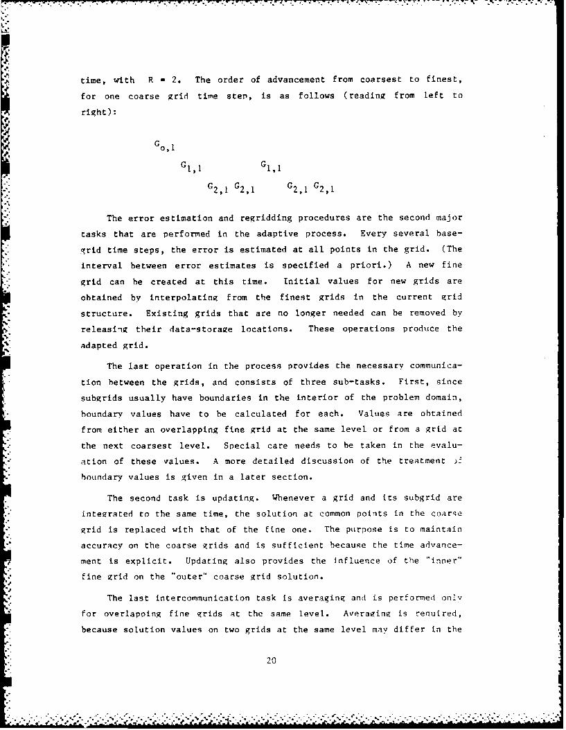
time, with R = 2. The order of advancement from coarsest to finest,
for one coarse grid time step, is as follows (reading from left to
right):
Go,1
GI, GI,
G2 ,1 G2 ,1 G2 ,1 G2 ,1
The error estimation and regridding procedures are the second major
tasks that are performed in the adaptive process. Every several base-
grid time steps, the error is estimated at all points in the grid. (The
interval between error estimates is specified a priori.) A new fine
grid can be created at this time. Initial values for new grids are
obtained by interpolating from the finest grids in the current grid
structure. Existing grids that are no longer needed can be removed by
releasing their data-storage locations. These operations produce the
adapted grid.
The last operation in the process provides the necessary communica-
tion between the grids, and consists of three sub-tasks. First, since
subgrids usually have boundaries in the interior of the problem domain,
boundary values have to be calculated for each. Values are obtained
from either an overlapping fine grid at the same level or from a grid at
the next coarsest level. Special care needs to be taken in the evalu-
ation of these values. A more detailed discussion of the treatment )f
boundary values is given in a later section.
The second task is updating. Whenever a grid and its subgrid are
integrated to the same time, the solution at common points in the coarse
grid is replaced with that of the fine one. The purpose is to maintain
accuracy on the coarse grids and is sufficient because the time advance-
ment is explicit. Updating also provides the influence of the "inner"
fine grid on the "outer" coarse grid solution.
The last intercommunication task is averaging and is performed onlv
for overlapping fine grids at the same level. Avkeraging is renuired,
% because solution values on two grids at the same level may differ in the
20
w...........* . . . . . . . . --.-
overlapping region. The solutions on each grid in the overlap are re-
placed by the averaged values.
To summarize the adaptive procedure, the solution is advanced for a
specified number of coarse-grid time steps. The error is then estimated,
and the grid is adapted. The special grid intercommunication procedures
are performed during both of these processes. After the grid is adapted
and initialized, the solution can then be advanced again.
2.4 Error Estimation
Subgrids are placed over regions that need refinement. As stated
earlier, a grid is refined where the truncation error is large. In this
method, a variation of Richardson extrapolation is used to estimate the
truncation error. In this section we show how the truncation error
estimate is calculated and point out the advantages of this technique.
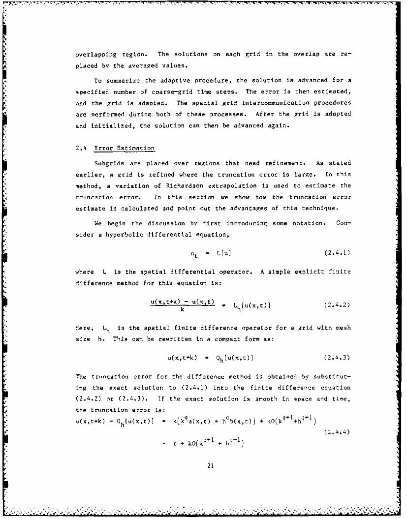
We begin the discussion by first introducing some notation. Con-
sider a hyperbolic differential equation,
ut a L[u] (2.4.1)
where L is the spatial differential operator. A simple explicit finite
difference method for this equation is:
u(x,t+k) - u(xt) . L [u(xt)J (2.4.2)kh
Here, Lh is the spatial finite difference operator for a grid with mesh
size h. This can be rewritten in a compact form as:
u(x,t+k) Qh[U(X,t)] (2.4.3)
The truncation error for the difference method is obtained by substitut-
ing the exact solution to (2.4.1) into the finite difference equation
(2.4.2) or (2.4.3). If the exact solution is smooth in space and time,
the truncation error is:
u(x,t+k) - Oh[u(x,t)] - k(kqa(x,t) + h0 b(x,t)) + kO(k+l +h
q+I)
(2.4.4)
- T + kO(kq+ l + h
21
+* . . -i - - + . . . . . . . .. . . . . . . . . ... . . . . + .

where T is the leading order term. Note that that the order of
accuracy of the method in space and time are the same and equal to q.
Taking two consecutive time steps with the method gives
u(x,t+2k) - Qh[u(xt)] . 2T + kO(kq+l+h q+l) (2.4.5)
Let Q2h represent the same difference method as Qh except with mesh
size 2h and time step 2k. The truncation error for the 2h - 2k
method is:
u(x,t+2k) - 0 2h[U(X,t)] 2k L(2k)qa(x,t) + (2h)qb(x,t)
+ kO(kq+l+h q+l) (2.4.6)
2q(2T) + kO(kq+l+hq+l)
* Neglecting the higher-order terms in (2.4.5), subtracting (2.4.6) and
dividing by 2 (2q-1 ) gives:
Q2fu(xt)] - Q2h[u(x,t)] + +l h+lh T + kO~k +hqJ (2.4.7)
2(2 -)
(2.4.7) provides an estimate of the leading term in the truncation
error.
This is equivalent to advancing the solution two steps from time t
with the standard method and comparing it with the solution obtained by
taking one double-step on a 2h mesh. This is illustrated schematic-
ally in Fig. 2.4 for a simple explicit method which uses U(xh,t) ,
u(xt), and u(x+h,t) to evaluate u(x,t+k).
A major advantage of this technique is that the exact form of the
truncation error does not need to be known. For many differential equa-
tions, especially systems, the exact truncation error can be very com-
plex and tedious to derive. The method is also independent of both
differential and difference equations and therefore can he applied to a
wide variety of problems without difficulty, in contrast to global re-
finement techniques which use heuristic error measures that are problem-
dependent. The error estimation is also relatively inexpensive.
22
*~..a.~.* -. a*-~ *~~*.9 >* 99~~9 > ~ • -

* - . .- - - 7-
When it is time to estimate the error, (2.4.7) is evaluated at
every point in the grid. If the pointwise truncation error estimate is
greater than a prescribed value, the point is "flagged" to denote that
refinement is needed in its vicinity. Once all the local error estimates
have been calculated and checked, the collection of flagged points is
then processed to generate the next level of refined subgrids.
2.5 Refined-Grid Generation
This section describes the procedure for generating refined grids
to enclose a collection of flagged points. We discuss only the proce-
cure used in two dimensions, as it is trivial in one dimension.
Grid generation is done in two steps. Flagged points are separated
or clustered into spatially distinct groups. Individual clusters are
then "Fit" with the rectangles of arbitrary orientation. The "goodness
of fit" is evaluated for each rectangle. If a rectangle has a bad fit
(encloses too much of an area not requiring refinement), it is broken
into subclusters that are refit with new rectangles.
Clusters are created with an algorithm which requires all points in
a cluster to be near neighbors. A new cluster is begun by assigning one
point to it. Other points are added to the cluster if their distance
from any point in the cluster is less than a specified value. The in-
tercluster distance is a small integral number of mesh widths.
Each cluster is then fit with an ellipse determined in the follow-
ing manner. Let matrix A be the n x 2 matrix of the coordinates of
the points relative to their mean (xmYm), n the number of points in
the cluster, and
Then the 2 x 2 matrix M - ATA is:
23

h
2 2 x x y~ - Xymx i -xm m
M =
2 2x i - x Y Y i Y m e
and contains the second moments of the points about their mean. M is
symmetric and has real eigenvectors which are easily calculated and de-
fine the major and minor axes of an ellipse. The sides of the rectangle
are determined by requiring that all points be contained in it.
The measure of goodness of fit is the ratio of the number of
flagged points to the total number of coarse grid points enclosed by the
rectangle. If the ratio is too small, the cluster is then processed
into subclusters using a more sophisticated routine. We do not describe
this method, since we have found the nearest-neighbor algorithm to per-
form sufficiently well for elliptic problems.
Before closing this section, we mention that this grid-generation
technique can be easily extended to three dimensions. The nearest-
neighbor algorithm would be unchanged. M would become a 3 x 3 matrix
describing an ellipsoid.
2.6 Boundary Values for Refined Grids
Special care needs to be taken in specifying boundary values for
the subgrid boundaries that are interior to the problem domain. Fine-
grid boundary values are generally interpolated from the coarse-grid
solution; accuracy must be maintained at the internal grid boundary.
For time-dependent problems, the interpolated values must not destroy
the stability of the time advancement. If the differential equation
represents a conservation law, it is also desirable to maintain conser-
vation at the boundary. We discuss how each of these concerns was
addressed by Berger's method.
In one dimension, the boundaries of the fine grids are made to
coincide with coarse-grid points. When both coarse- and fine-grid
solutions have been integrated to the same time, there is no ambiguity
in the choice of fine-grid boundary conditions. However, the fine grid
also requires boundary conditions at intermediate times, since it is
24
Z. ..
.7 -7

advanced R times for each advancement on the coarse grid. Berger used
linear interpolation in time, whose accuracy is consistent with the
time-difference method. Higher-order interpolation would have required
the storage of solution values from previous time steps.
In two dimensions, the interpolation was bilinear in space and lin-
ear in time. This method was found to provide sufficient accuracy, in
part because internal boundaries were normally located where the solu-
tion was slowly varying.
Berger analyzed the stability of the time interpolation. With the
Lax-Wendroff difference method applied to the linear wave equation in
one space dimension, it was shown that these boundary conditions were
stable. Numerical experiments with other hyperbolic equations in one
and two dimensions showed no loss of stability.
For hyperbolic conservation laws in one dimension, it is well known
that difference schemes that exactly conserve fluxes of the dependent
variables can he guaranteed to converge to the correct shock speed and
jump condition. Therefore, conservative methods are commonly used in
shock calculations. When an internal grid boundary is introduced in the
domain, special treatment must be applied to grid points along the
boundary in order to maintain conservation, especially if a shock is
located in the vicinity of the boundary. To preserve conservation, the
flux into the grid boundary should exactly equal the flux out of it.
Conservation can be imposed in two ways. Either the boundary conditions
are specially evaluated, or the difference equations for the boundary
points are modified to preserve the correct flux balance.
Berger derived conservative and stable boundary-difference formulas
for use with the one-dimensional wave equation. It is not clear whether
these conditions were used; however, it was not critical for the calcu-
lations shown, since shocks were always located away from internal grid
boundaries.
Analysis was not done for two dimensions; due to the rotation,
coarse and fine grid points will not coincide. Berger points out that
spatial, bilinear interpolation is not conservative. However, her
results indicate that accutracy was maintained.
25
. .. . . . .. . . . . . -..
S-- - - .

Finally, we note that it would be difficult to implement modified
boundary-difference equations for arbitrarily rotated grids. Conser-
vative difference equations using fine and coarse grid points would be
difficult to construct, given the arbitrary rotation. It is more
straightforward to interpolate the boundary values in a conservative
manner.
. 2.7 Data Structures
Because of the complexity of Berger's system of grids, non-standard
" data structures were used to describe the grid hierarchy and to store
grid-solution vectors. We describe these structures in this section.
The purpose of the grid data structure is to describe each grid and
its relationship to other grids. For example, the information stored in
the data structure determines which coarse grid to interpolate boundary
conditions for a fine grid, the order of integration of the grids, where
the solution vector for a given grid is located, etc. The grids are or-
ganized in a tree-like structure. An illustration of a two-dimensional
tree structure is given in Fig. 2.5. The tree is constructed by keeping
track of the local relationships that are indicated by the double arrows
in the figure.
Before describing the tree, we introduce some definitions. Sub-
grids of the same parent coarse grid are called siblings. Subgrids are
called neighbors if they are at the same level of refinement but have
different parents.
Each grid is treated as a node in the tree; its description is
stored as a fixed-length vector. To distinguish them, the nodes are
numbered. They contain a complete description of the grid; information
stored includes:
1. Grid location (coordinates of its corners).
2. Number of grid points.
3. Mesh sizes.
4. Level in tree.
5. Parent.
6. Offspring.
26
..................................................... ..,.....

7. Previous neighbor on level.
8. Next neighbor on level.
9. Time to which grid has been integrated.
10. Index in main storage array where solution is stored.
A parent can have more than one offspring, and a subgrid can have
more than one parent (for example, G3 ,1 in Fig. 2.5). Since node
vectors contain a fixed number of elements, a linked list is used for
data storage if a grid has multiple relatives. In that case, the node
entry for the parent or offspring points to the beginning of the string
of relatives that is located in the linked list. A description of the
linked list and its implementation can be found in any standard computer
science text on data structures.
This grid structure makes feasible an otherwise unwieldy data-
management problem and is partly responsible for the overall efficiency
of the adaptive method. The structure is dynamic in that grids can be
added or deleted from the tree during program execution.
The storage of grid-solution vectors also must be dynamic. Grids
created during the adaptive process require a location to store solu-
tions. Also, the area occupied by solutions for grids that are de-
stroyed should be reclaimed for future use. If this is not done, the
program's memory requirements could exceed the computer's limit during a
run. FORTRAN does not permit dynamic dimensioning of arrays, so a
special data structure to handle the solution vectors was developed.
A single, large, global array is allocated for storing all solu-
tions and any temporary work space that is required. When a grid is
created, space is reserved in this array for its solution. The begin-
ning address in the array is saved in the node vector. When a grid is
destroyed, its space is reclaimed. Because of the dynamic nature of the
creation and destruction of grids, storage in the global-solution array
will not be contiguous. The location and length of free blocks in the
array is maintained in a linked list. When a grid is created, the list
is searched to find an appropriate location to store the solution. When
a grid is deleted, its solution storage area is added to the list of
free blocks.
27

Fig. 2.1. Overlapping, component grids.
G o,1
Fig. 2.2. Example of overlaid grid structure.
-' 28

k2k
t,2k
t+k
t
X-2h X-h X h X*h2h
Fig. 2.4. Richardson ex~traPolatio f'or time-explicit miethod.
29

G 0 G, 2
G2,01
Fig. 2.5. Tree data structure
30
W-e
N11.- . .

Chapter 3
STRATEGY FOR ELLIPTIC EQUATIONS
3.1 Overview
In this chapter, we describe how Berger's refinement approach is
applied to elliptic flow problems. The differences prevent direct ap-
plication of Berger's method. Our strategy was to implement the fol-
lowing two features of the method:
* overlaid, locally uniform grid refinement consisting of rotated
rectangles, and
* refinement regions defined by Richardson error estimates.
Thus, Berger's grid-generation algorithms and data structures, described
in Chapter 2, are used in our program.
In the next section, we discuss how the characteristics of elliptic
equations influence the choice of the method. The differences between
elliptic and hyperbolic flows are highlighted. We then develop two
adaptive strategies, active and passive. Discussions of the error-
estimation methods and treatment of initial and boundary conditions for
refined grids follow.
3.2 Influence of Elliptic Equations on Adaptive Approach
The flows we are interested in are governed by the steady, incom-
pressible, laminar or Reynolds-averaged Navier-Stokes equations. These
systems are elliptic in contrast to the Euler equations, which are
hyperbolic, and the boundary-layer equations, which are parabolic.
Elliptic flows are characterized by thin regions (boundary and
free-shear layers), in which the velocity has a rapid variation in the
direction normal to the main flow direction. This contrasts with hyper-
bolic flows which contain shocks, in which the rapid variation occurs
over infinitesimally small regions aligned with or oblique to the main
Flow direction. Within shear layers, viscosity or turhulent diffusion
is important.
31

Outside the thin shear layers (TSLs), the velocity varies smoothly,
the effects of viscosity are small, and the flow is determined primarily
by a balance between inertia and the pressure gradient. Viscosity can
often be completely neglected in these regions.
Fine grids are needed in the vicinity of TSLs; coarser grids suf-
fice for the outer flow. The locations and sizes of TSLs are usually
not known in advance, and may depend on the Reynolds number. An adap-
tive method must he able to "recognize" the TSLs so that the refinement
grids can be correctly located.
Elliptic flows may also have recirculating regions, in which the
local flow direction is opposite to the main flow. Due to recirculation
and the long-range effects of pressure, influences may be felt both
upstream and downstream. In hyperbolic and parabolic flows, influence
occurs only in the downstream direction.
Because information propagates differently, different solution
methods are used for each type of flow. For hyperbolic and parabolic
flows, the solution is generated by marching in the flow direction.
With elliptic equations, large regions of the flowfield require simul-
taneous solution. This requires modification of the adaptive method
used for hyperbolic equations.
3.3 Two Adaptive Strategies
In this section, we develop two methods; each is applicable to a
class of elliptic flows. Overlaid grid refinement is used in both
cases; they differ primarily in how the solutions on the various grids
rplate. Also, each uses a different error criterion. The classifica-
tion of flows is discussed first. We then outline the two adaptive
strategies and their solution and error-estimation procedures. The
methods are described in detail in later sections.
When the shear lavers are thin, the outer flow depends only weakly
on the properties of the shear layers. The flowfield in each region can
be qtudied independently to a good approximation (Mehta, 1984). Such a
flow is described as having a weak viscous-inviscid interaction.
32

When shear layers are not thin, there is stronger coupling between
the inner and outer flows. Local effects within the shear layer may
then have long-range, multidirectional influence. The coupling is
provided by the pressure gradient and recirculation. These flows are
said to have strong viscous-inviscid interation; the inner and outer
regions cannot be analyzed independently.
Consider a concrete example - incompressible, viscous flow over an
airfoil at a high Reynolds number. So long as the boundary layer re-
mains attached, it is thin and exerts a weak influence on the outer
flow. The latter can be accurately calculated by either neglecting the
boundary layer or using a crude approximation to it. Given an accurate
outer flow, the boundary layer can be calculated to a good approxima-
tion. However, if the boundary layer separates, it can thicken consid-
erably and there may be significant modification of the outer flow. In
this case, the two parts of the flow field must be calculated simul-
taneously.
Different solution-adaptive strategies were developed for these two
types of interactions.
For flows with weak interactions, the outer solution does not need
to be recalculated, as the accuracy of the calculation of the shear
layer is improved through grid refinement. The "passive" adaptive
method is formulated to take advantage of this.
In the passive scheme, an initial calculation is made on a coarse
grid and its error is estimated. Refined grids are then constructed so
that they enclose the inaccurate region(s). Care is taken to ensure
that their boundaries be in accurate regions, so that accurate boundary
conditions can be taken from the initial solution.
Solutions are then calculated on the refiner grid regions, and
their errors are estimated. If necessary, a new level of refined grids
is created. The procedure is repeated until further refinement is no
longer necessary.
At any step, the solution is calculated only on the most recently
created, finest level grids. The outer solution is never recalculated;
it assumes a "passive" role in the adaptive process. Since the outer
33

*~~~~~~ .r . .- . .'* .. . . .. .-.----- ..-. .
solution is not recalculated, its error, rather than the truncation
error, must he used as the basis for a refinement criterion. This is an
outline of the passive scheme; details will be given later.
For flows with strong interactions, the inner and outer solutions
have to be calculated simultaneously. Improving the solution in the
shear layer changes the flow in the outer region. The "active" scheme
is formulated for these flows.
In the active scheme, an initial solution is calculated on a coarse
grid, as in the passive method. Since the initial grid is coarse, the
strong interaction causes the outer solution to be inaccurate. The
solution is likely to be inaccurate everywhere, so the solution error is
not a good indicator of where refinement is required. For this reason,
the local truncation error is used as the basis for the criterion for
refinement in the active scheme.
Refined grids are constructed to enclose regions of large trunca-
tion error. The coarse-grid solution provides boundary conditions for
these grids, and the solution is calculated on them.
However, the coarse grid solution has to be recalculated to account
for the change in the inner solution. This is done by modifying the
coarse-grid equations to account for the improvement provided by the
fine grid, then recalculating the coarse-grid solution. New fine-grid
boundary conditions are obtained from the new coarse-grid solution, and
the fine-grid solution recalculated. This procedure is repeated until
the solution no longer changes on either grid. In this method, the
coarse grid "actively" participates in the solution procedure.
The choice of which strategy to use, active or passive, depends on
the strength of the coupling between the flow within the TSLs and the
outer flow. For simple flows, the strength can be determined.
For flows along solid surfaces, the coupling is due to the dis-
placement of the outer flow by the boundary layer. The strength of the
interaction can be quantified. This was done for the developing bound-
3rv layer in a plane channel (shown in Fig. 3.1). We outline the analv-
sis here; details are given in Appendix A.
34
.. . . . . . . . . . . . . . . . . . . . . % i; .. .

The velocity V0 in the inviscid core region can be related to the
displacement thickness, 6*. Let the change in 6* be:
A6 = (K-1)6*
where K is a sensitivity parameter. On a coarse grid, the boundary
layer may be smeared to twice its actual size, K = 2. Figure 3.2 shows
the relative change in V0 as a function of 6* /L for K - 2 and 10,
where L is the channel width.
The relative change in V0 should be no greater than the maximum
allowable error. For K - 2 and maximum allowed relative error, 0.1%,
the displacement thickness should be 6 /L < 10- At larger 6 /L,
the coupling is stronger. The passive method should be used for
6 */L < 10-3; the active method is required for larger 6 */L.
This concludes the outline of our adaptive strategies. To summa-
rize, we have shown that elliptic flows having strong and weak viscous-
inviscid interactions require different adaptive strategies, and we have
developed these strategies.
In the next two sections, we describe each strategy in more detail.
3.4 Passive Method
3.4.1 Strategy
In this section, we describe the algorithm for the passive strat-
egy, which is applicahle to flows having weak viscous-inviscid interac-
tions. We also present some theoretical results that justify the
technique.
The passive method is begun with the calculation of a converged
solution on the coarse grid. The error in this solution is then
estimated, using the method described below in Section 3.7. Regions
having large estimated solution error are fit with refined grids, as
described in Section 2.5. Boundary conditions and initial guesses for
refined grids are interpolated from the coarse-grid solution. The
solution is then calculated on all newly created refined regions (see
Fig. 3.3). A soecial procedure is required to calculate the solution on
a set of overlapping grids; it is described in Section 3.6.
*35

The solution is not recalculated outside the refined regions in
this method. Boundary values for the refined region remain fixed during
the computation. For safety, each newly created rectangle contains a
buffer zone, which is usually one or two coarse mesh widths wide on all
sides.
After the solution and its error estimate have been comouted,
refined grids are generated. These grids usually lie within the bound-
aries of the previous grids, but they are not required to do so. Bound-
ary conditions are taken from the next coarsest grid on which data are
available.
Thus, the passive solution method is described by:
(0) Set up base grid, GO; k = 0.
(1) Calculate solution on Gk.
(2) Estimate solution error on Gk.
(3) Check for convergence.
(4) If converged, stop; otherwise continue.
(5) Generate refined grids, Gk+.
(6) k k + 1; go to (1).
Convergence is achieved when the estimated solution error (maximum abso-
lute value or rms) falls below a specified value.
3.4.2 Summary of Theoretical Results
Theoretical justification for this solution technique can be found
in analyses of one-dimensional boundary-value problems. We shall summa-
rize these results.
The solution to the two-point boundary-value problem for the ordi-
nary differential equation:
-y'" + p(x)y' + q(x)v = f(<)
y(O) - y ; v( ) = Y (3.4.1)
p(x) > 0 ; q(x) > 0
36
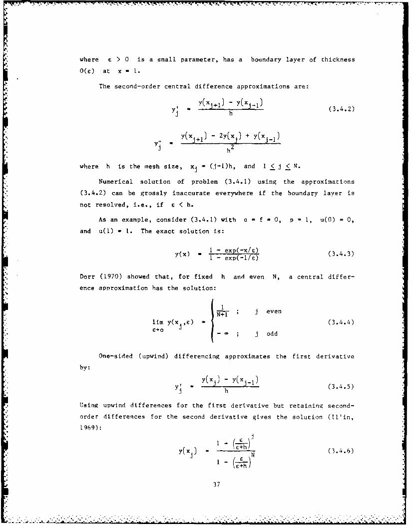
where e > 0 is a small parameter, has a boundary layer of thickness
0(N) at x .
The second-order central difference approximations are:
Y(XJ+l) - y(x 1 _)" h (3.4.2)
- Y(xj,) - 2y(x ) + y(xj_ 1 )y h 2
where h is the mesh size, xj - (j-I)h, and I < j < N.
Numerical solution of problem (3.4.1) using the approximations
(3.4.2) can be grossly inaccurate everywhere if the boundary layer is
not resolved, i.e., if e < h.
As an example, consider (3.4.1) with a f = 0, p 1, u(0) = 0,
and u(1) = 1. The exact solution is:
y(x) = 1 - exp(-x/e)1 - exp(-I/e) (3.4.3)
Dorr (1970) showed that, for fixed h and even N, a central differ-
ence approximation has the solution:
N+- ; j even
lim y(x ,e) = (3.4.4)Sj odd
One-sided (upwind) differencing approximates the first derivative
by:
y(xj) -y(xj_)
Yi = h(3.4.5)y1 h
Using upwind differences for the first derivative but retaining second-
order differences for the second derivative gives the solution (ll'in,
1969):
y(xj) = N (3.4.6)
37

The solution (3.4.6) behaves like the exact solution (3.4.3) away from
x - 1. However, the boundary layer is several mesh widths thick. Thus,
it is smeared unless h < e, i.e., unless the grid is find enough.
Kellog and Tsan (1978) derive error bounds for solving (3.4.1)
using upwind differencing. Their results show that the error in the
boundary layer does not pollute the solution away from x = 1. For our
adaptive method, this means (at least for this problem) that we do not
have to re-solve the problem on the coarse grid as the boundary layer is
refined, if upwind differences are used. Our experience shows that the
technique works in both one and two dimensions (see Chapters 4 & 5).
For p < 0, (3.4.5) must be replaced by:
Y(xj+) - y(xj)YJ (3.4.7)
Yj h
3.5 Active Method
The active technique is used for problems with strong viscous-
inviscid interactions. We describe the active algorithm in this sec-
tion.
In this strategy, the grid-refinement process is similar to the one
used in the passive strategy, with two major differences. First, the
solution is iterated over all refinement levels after a new level of
grids has been added. Second, the refinement is based on local trunca-
tion error estimates rather than solution error estimates (cf. Section
3.3). The method used to estimate the local truncation error is given
in Section 3.7.
Because the coarse solution is updated in the active method, we do
not need to be as conservative in refining the grid. Thus, the error
tolerances used to define the refinement regions may be larger, and
huffer zones for refined grids may be smaller.
Consequently, an active calculation generates smaller refined grids
than a passive calculation of the same problem. However, the active
calculation may not be more efficient, since additional work is expended
in updating the outer solution. The relative efficiency of the two
methods depends on the strength of the coupling between outer and inner
38
-7 -

solutions. The passive method is better for weak coupling, the active
method for strong coupling. It is difficult to determine a priori which
method is more appropriate for a problem with an intermediate-strength
coupling; it is safer to use the active strategy in such cases.
We shall describe the active method for generating the solution onthe two-level svstem shown in Fig. 3.4. Extension to more levels is
straightforward.
Assume we have the differential equation (written in operator
form):
Lu = f (3.5.1)
on the domain, a, with appropriate boundary condiLions. L is the
differential operator.
We want to solve (3.5.1) using the two-level grid system indicated
in Fig. 3.4. The coarse grid Go covers 00 and has mesh size H.
The fine grid G1 covers S1 and its mesh size is h. Note that
H = Rh, where R is the refinement ratio.
We use the same difference approximation on both grids; only the
mesh size differs. The approximation on the coarse grid is represented
as
LHuH = f (3.5.2)
and on the fine grid as:
LhUh = f (3.5.3)
We want the solution to satisfy the fine grid approximation on Ql, the
coarse grid approximation on S1 -Q1 and the solutions on the two
grids should agree at common points, i.e., on Q11
In other words, the solution should satisfy:
LhUh = f on Q (3.5.4a)
L"uH = f on Q 0 Q (3.5.4b)
u4= uh on Ql (3.5.4c)
39

.,,
The last condition requires that the coarse grid equations be modified
in al. Equations (3.5.4b) are solved on Q o - al while the equa-
tions:
LlHuH = LHuh (3.5.5)
are solved on Q1. The terms on the right-hand-side are the "coarse
grid corrections terms". Solution of this equation gives the desired
result (3 .5.4 c).
Assuming that the grids have been selected, the following procedure
is used to generate the solution. An initial coarse grid solution iq
first calculated on the entire domain, i.e., LHuH = f is solved on
a0. Boundary conditions for the fine grid are interpolated from this
solution, and a fine-grid solution is calculated. The coarse grid cor-
rection terms are then calculated, using the current fine grid solution.
The modified coarse grid equations are solved, boundary conditions are
then interpolated for the fine grid, the solution calculated on the fine
grid, and so on. Convergence is achieved when the interpolated fine
grid boundary conditions no longer change.
Thus, the active solution algorithm is:
(0) Calculate initial coarse grid solution; solve:
0LH H N = f (on Q O 0 m = I
(1) Update boundary values for G1 by interpolating solution on
G:0 u m ( m 1 (_
hI) uH
(2) Check for convergence, e.g.,
maxluh(Yl)- Uh' 1(y) < E
Yl(3) If converged, stop; otherwise continue.
(4) Calculate fine grid solution; solve:
mLhuh = f (on Q
(5) Calculate coarse grid correction:
L u MH h
40

(6) Calculate coarse grid solution; solve:
L Lu on QLHU H =LUL H -H Hf o n Q o - S1I
(7) Go to (1).
Corrections are applied at coarse grid points internal to the fine
grid. Coarse-grid points lying on the fine grid boundaries are not
corrected, permitting the solution on the fine grid boundaries to change
as the solution converges.
For one-dimensional problems, calculation of the correction is sim-
ple, since coarse and fine grid points are coincident. With rotated
grids in two dimensions, the fine grid solution has to be interpolated
to evaluate the correction terms. This is done as follows. The coarse-
grid difference approximation (3.5.2) at a point (i,j) on a uniform
rectangular coarse grid, Go, can be written:
a H + b H
LHuHJ = aij(uH)ij + ij(ui+' cijuHi-J (3.5.6)H - H
ii(uH) + eij(uHij
for the five-point stencil shown in Fig. 3.5. We have assumed that the
equation is linear and the coefficients a, b, c, d, e are known, for
the purposes of illustration. (The procedure is equally applicable to
nonlinear equations.) The correction terms in (3.5.6) are formed by
replacing the uH's in the stencil by the corresponding fine grid
values, i.e.:
L i. a H + H -'
h aii(uh)ij + bij(uh)i+liJ + cij(uh)i-.'J
H H+ d.u + e ()
ij(Uh)ij+l ij(Uh)ijl
The location of the coarse grid point (i,j) determines which solution
values (coarse or fine) are used. Four cases are indicated in Fig. 3.5.
41
-i " *'- - . * ' 7 ' ' . . . .. . . . . . . . . . . ....-. "-,"
.S", ", , -' , - h - . - ..- '4%I*- . "•
.. C '... C

In case (i), all five coarse grid points are internal to the fine grid,
GI; the fine grid solution is used at all five points. In the second
case, (i+l,j) and (i,j-l) lie outside the fine grid. The coarse
grid values are used for these, the fine grid, for the other three. In
case (iii), the point (i,j) lies on the boundary of G1 . The correc-
tion term is not needed here nor for case (iv), for which the stencil is
completely outside the fine grid domain.
This concludes our discussion of the active solution method for the
two-level grid system; the method is easily generalized to more than two
levels. Correction terms are applied on grid Gk, if there is a finer
grid Gk+1* However, the solutions on the various grids are generated
successivelv, going from coarsest to finest and back again. One itera-
tion is defined as solving on the grids in the order:
G1, G2 9 " Gkmax Gkmax-' ' Go
where Gk is the grid on the finest refinement level. This "V"kmax
sweep pattern is also used in multigrid methods.
To summarize, the major difference from the passive method is that,
in the active method, information is passed from the fine grid to the
coarse grid and the solution is generated on both grids simultaneously.
Also, the truncation rather than the solution error is used to define
the refinement regions.
" 3.6 Solution on Overlapping Grids
On a given level, Berger's method may generate overlapping grids to
enclose a cluster of flagged points. An example having two such grids
is shown in Fig. 3.6.
Assuming that boundary conditions are specified, except in the
overlap region, the problem is to solve a houndary-value problem on an
irregular domain. A numerical version of the Schwarz alternating
method, outlined below for the case of two rectangles, is used; it can
be extended to more rectangles.
The problem domain, Q, is composed of two overlapping rectangular
subdomains, S1 and Q2, as indicated in Fig. 3.6. r1 and r242
7-* . . . . . . . . . .
* .P.. .. * .

denote the boundaries of the two rectangles; Y1 and Y2 are their
internal boundaries.
Boundary conditions are specified on the external boundaries,
(ri - yi), i - 1,2. The initial conditions on the internal bound-
aries, yl, are guessed (or interpolated from a coarse grid solution)
and the following algorithm is carried out.
(1) Update internal boundary values on y1 from the solution onn n-i(r2 : u'(y1) U This usually requires interpolation.
(2) Solve for ul(x,y) (on Ql) .
(3) Update internal boundary values on Y2 : un(Y2) = (YI)'
again by means of interpolation.
(4) Solve for un(x,y) (on S2).
(5) Check for convergence, e.g.,
maxI uu7 Ci i
Yi(6) If converged, stop; otherwise go to (1).
The Schwarz alternating method has been analyzed for simple ellip-
tic equations (including Laplace's and Poisson's) on unions of simple
subdomains. Some of the relevant results are summarized next.
The technique was originally developed to prove the existence of
continuous solutions to the Laplace-Dirichlet problem on irregular
regions. (See Stoutemyer (1972) for a review of the early literature.)
However, assuming the existence of a continuous solution, the conver-
gence of the discrete solution can be guaranteed for certain classes of
problems. Miller (1965) shows that two additional conditions are suf-
ficient for convergence. They include:
(1) the discrete approximations must converge to the continuous
solution as the mesh size goes to zero;
(2) subregion approximations must satisfy the maximum principle on
their respective domains (i.e., the solution error on each
subregion must be less than the error on the internal bound-
aries. This condition is satisfied by many elliptic equa-
tions.)
43
2... .............. . •.".•. ..- . .-..-. . ..... . . . .- '-" I" -N %V. " . *:"." ." . . . .

Miller showed that, at the nth iteration, the error on the internal
boundaries converges linearly:
le iyII q njle'll i = 1, 2
where 1< l~l~yidenotes the maximum value along the boundary Yj' and
Iqi < 1. Convergence can be accelerated using standard techniques,
e.g., Aitken's method (see Smith, 1978), SOR (successive overrrelaxa-
tion), etc. The magnitude of q is problem-dependent; it depends on
the amount of overlap, the geometry of the subdomains, etc.
Miller also analyzed the case in which the numerical solution on
each grid is not carried to convergence at each step. He found bounds
on the error made on the internal boundaries in terms of the error at
internal points and thus established stability. However, the conver-
gence rate could not be determined, since it depends on the numerical
method and the degree of solution convergence on each subregion. All of
Miller's results apply to both linear and nonlinear problems.
Rodrigue and Simon (1983) analyzed a method for solving elliptic
equations on multiprocessor computers. They decomposed the domain into
subregions, each of which was assigned a single processor. The Schwarz
alternating procedure was used to compute the solution on the complete
domain. The method was recast as a matrix problem so that classical
techniques of acceleration could be applied (see e.g., Hageman and
Young, 1981). For linear problems, they showed that the procedure is
equivalent to the block Gauss-Seidel iterative method. Numerical
experiments with Laplace's equation showed that the convergence rate
increased with increased overlap area.
Tang et al. (1985) analyzed the Schwarz method for Poisson's
equation in n-dimensions when the problem domain is a line, rectangle,
or box in I-D, 2-D, and 3-D, respectively. The domain was composed into
an arbitrary number of strips, each having the same size and amount of
overlap. The convergence rate was linear, but depended on the overlan
area and the number of strips. SOR applied to the internal boundary
values was shown to sneed up convergence. Formulas were given for the
optimum relaxation factors. Numerical results agreed with the theory.
44

Kang et al. (1985) consider the Schwarz alternating procedure with
multiple subregions on parallel computers. They demonstrated conver-
gence independent of the order of solution on the subregions. They also
showed that an energy norm of the error monotonically decreases.
A practical application of the Schwarz method is given in Atta and
Vadyak (1983). Transonic external flow calculations were made using
overlapping, three-dimensional grids. Two overlapping component grids
were used. Multivariate quadratic interpolation was used to update
internal boundary values. Starting from an initial specified field,
each grid was iterated a fixed number of times before boundary values
were transferred. Convergence was achieved after 10-15 Schwarz itera-
tions.
3.7 Error Estimation
In the passive technique, we need to determine where the coarse
grid solution is accurate. We keep that part of the solution, and
refine and re-solve only where the error is large.
In strongly coupled problems, the solution, or global, error is
spread over the domain by convection and diffusion. Consequently, it
may not he a good indicator of where grid refinement is required.
Therefore, in the active method, the local truncation error is used to
define refinement regions.
In this section we present the methods used to estimate the solu-
tion and truncation errors. We then discuss how the two errors interact
in elliptic flows.
We use a form of Richardson extrapolation to estimate both types of
error. This technioue assumes that the solution error can be expressed
as a Taylor series
e(h,x) - u(O,x) - u(h,x) - hPF(x) + hqG(x) + ... (3.7.1)
where u(O,x) is the exact solution, h the mesh size, and p the
order of the method (p - 2 for second-order methods). This expansion
is valid for smooth solutions with several continuous derivatives -- a
condition that is satisfied by all elliptic flows.
45
-1. . . . .

--
If we double the mesh size (for both cootdinates in two dimensions)
and calculate another solution, the error becomes:
e(2h,x) - u(O,x) - u(2h,x)(3.7.2)
- 2PhPF(x) + 2qhqG(x) +
Subtracting (3.7.2) from (3.7.1) and dividing by 2P - 1 gives an
estimate of the solution error:
(h,x) - u(h,x) - u(2hx)
2p - 1 (3.7.3a)
- hPF(x) + h - [ G(x) +
Comparing (3.7.1) with (3.7.3a), we see that:
e(h,x) = e(h,x) + O(h q) (3.7.3b)
so the estimate is accurate to order q.
Next we derive the truncation error estimate. In operator form,
the difference method is:
Lh[u(h,x)] = f (3.7.4)
where Lh is the difference operator. The truncation error is defined
as the residual obtained by substituting the exact solution of the dif-
ferential eouation, u(O,x), into the difference equation, i.e.,:
T(h,x) = th[u(O,x)] - f
(3.7.5)
L h[u(O,x)] - Lh[u(h,x)]
If Lh is linear, the relationship between solution and truncation
errors is obtained by combining the definitions (3.7.1) and (3.7.5):
T(h,x) = Lh[e(h,x)] (3.7.6)
Consequently, for linear problems, the solution error estimate,
(3.7 .3a), can be substituted into (3.7.6) to yield an estimate of the
truncation error:
-(h,x) = Lh[e(h,x)] (3.7.7)
46
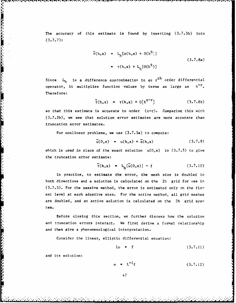
rrw
The accuracy of this estimate is found by inserting (3.7.3b) into
(3.7.7):
T(h,x) = Lh[e(h,x) + O(hq ' ]
(3.7.8a)
- T(h,X) + Lh[O(hq)]
Since Lh is a difference approximation to an r th order differential
operator, it multiplies function values by terms as large as hr.
Therefore:
•T(h,x) - T(h,x) + O(h -r) (3.7.8b)
so that this estimate is accurate to order (q-r). Comparing this with
(3.7.3b), we see that solution error estimates are more accurate than
truncation error estimates.
For nonlinear problems, we use (3.7.3a) to compute:
(O,x) - u(h,x) + Z(h,x) (3.7.9)
which is used in place of the exact solution u(O,x) in (3.7.5) to give
the truncation error estimate:
(h,x) - Lh[1(Ox)] - f (3.7.10)
In practice, to estimate the error, the mesh size is doubled in
both directions and a solution is calculated on the 2h grid for use in
(3.7.3). For the passive method, the error is estimated only on the fin-
est level at each adaptive step. For the active method, all grid meshes
are doubled, and an active solution is calculated on the 2h grid sys-
tem.
Before closing this section, we further discuss how the solution
and truncation errors interact. We first derive a formal relationship
and then give a phenomenological interpretation.
r, Consider the linear, elliptic differential equation:
Lu - f (3.7.11)
and its solution:
u L-If (3.7.12)
47

where L is the differential operator and L-1 represents its Green's
function.
Providing Lh can be inverted, from (3.7.4) we can also write:
u(h,x) = Lh 1f] (3.7.13)
Noting the similarity between (3.7.12) and (3.7.13), Lh can be
interpreted as a discrete Green's function (Gladwell and Wait, 1979).
We can also invert (3.7.6):
e(hx) - L-'[(h,x)] (3.7.14)
The numerical approximation (3.7.4) introduces the truncation error T;
(3.7.14) indicates how r is converted into the resulting solution
error. Note that the solution error is reduced by reducing the trunca-
tion error, i.e., by refining the grid.
We give an interpretation of how the error gets distributed in
elliptic flows. Consider the linear problem:
u(x,y) D + v(x,y) y V2 + S (3.7.15)
on a regular domain with Dirichlet boundary conditions. This equation
describes the convection and diffusion of a passive scalar * in a
known velocity field, given by u and v. S is a source of * in
the field.
A numerical approximation for this problem is:
u h hh 2h + S (3.7.16)
2where 6/6x, 5/6y, Vh are difference operators. This can also be writ-
ten:
Lhh S (3.7.17)
The solution error, eh = - h is related to the truncation error by
(3.7.6), which when expanded becomes:
48
-. . . . . . <- I............................

!e h + eh 2
uV e + T (3.7.18)6x 6y h h h (..8
We see that the solution error satisfies a discrete convection-diffusion
equation similar to (3.7.16), with eh - 0 on the boundaries. Th acts
as a source term. This shows that the solution error is convected and
diffused over the flow field in the same manner as *, and that its
source is the truncation error.
3.8. Initial Guesses and Boundary Values for Refined Grids
Since iterative solution methods are used, initial guesses are
required for newly created grids and the grids used for the error esti-
mates. For the former, initial guesses are interpolated from existing
grids. Guesses for 2h-grids are interpolated from the corresponding
h-grid solution. In both cases, bilinear interpolation is used.
The cell in the grid containing the point at which the guess is
needed is first found, as indicated in Fig. 3.7. The interpolated solu-
tion is found in terms of the local cell coordinates:
= i - io(3.8.1)
n- j - JO
where (io, jo) is the origin (see Fig. 3.7), and i and j are con-
sidered continuous variables. In these coordinates, bilinear interpola-
tion is:
u( ,n) -(1- )( - i) Uioj. + (l-n) uio+1 1j o0 (3.8.2)
+ n(1-0 + nui+1,j 0+1 Uo'Ji o'Jo+1
This second-order accurate method is sufficient for providing initial
guesses.
Boundary conditions for refined grids are interpolated from the
finest existing grids. These boundaries normally fall within the prob-
lem domain and are thus fictitious internal boundaries. Ideally, the
order of accuracy for interpolation at these locations should be at
least r + p, where r is the order of the differential equation and
49
------------....---- ---- -".-.-.-. . . ." .--. .-..... . "

p the order of accuracy of the approximation (Bai, 1984). This makes
the accuracy at the fictitious boundaries consistent with the accuracy
at other internal points.
To illustrate, assume we approximate the second-order equation
(r =2):
d u f (3.8.3)
dx2
with second-order central differencing (p = 2):
-2uj + u = f + O(h 2 (3.8.4)
h2 .
where we have indicated the leading term in the truncation error. Note
that Uj+l, uj, and uj_ are the exact solution values.
Also assume that we have to use an interpolated value u at some
point J inside the domain. uj d4 Ifers from the exact value uj by:
+ O(h) (3.8.5)
where q is the order of accuracy of the interpolation method. To see
how the interpolation error affects the difference approximation at the
point J, substitute (3.8.5) into (3.8.4) to get:
uj+I - 2( u + O(hq)) + uj+ = f + O(h 2) (3.8.6)
h2
Maintaining the same order of accuracy requires q > 4; cubic interpo-
lation would be satisfactory.
We used bilinear interpolation (similar to Berger's method) for
fictitious internal boundaries, primarily because of its simplicity.
Our experience indicates that the accuracy was sufficient for the prob-
lems investigated (see Chapter 5). However, a more acccurate method,
preferably cubic interpolation, is recommended, since it will increase
the adaptive method's efficiency.
Exact boundary values are used where refined grid boundaries are on
the computitional boundary.
50

For the Navier-Stokes equations, a conservative interpolation pro-
cedure was developed for internal fine grid boundaries. This method is
discussed in detail in Chapter 7.
In this chapter we have described how Berger's method was extended
to provide a method of solving the elliptic flow equations. New solu-
tion and error estimation procedures were presented, along with a dis-
cussion of the treatment of initial guesses and boundary values for
refined grids. We apply the method to one-dimensional problems in the
next chapter, and to a two-dimensional one in Chapter 5. Chapters 6 and
7, respectively, discuss the solution method and adaptive procedures
used with the Navier-Stokes equations. Results of adaptive calculations
for the Navier-Stokes equations follow in Chapter 8.
51
iI
';1
A
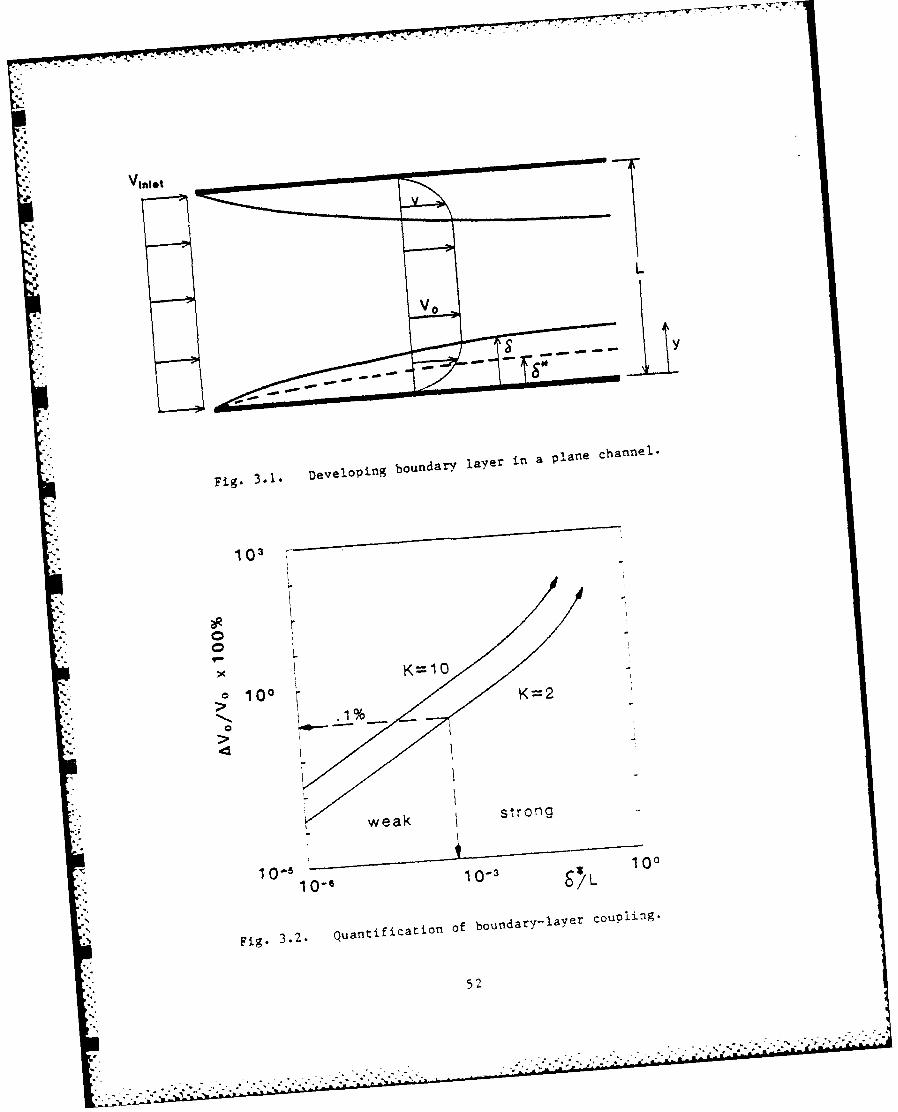
L
ov
K=10
100 K=2
'4
weak stronlg
0- 6 -
100
1 00-s
Fig. 3.2. Quanificaion of boufdarylayer
coupling.
52

set of overlapping grids
Isolated grids
Fig. 3.3. Example of newly refined regions.
0I
Grid G
)Y1Grid G o J
O 0
Fig. 3.4. Notation for active solution on two-level grid system.
53
. .. . '..-. .. % ,, .-. " . .' . % . . .' "-.- - . . o .. .-. . . .. . . .. . . .. .. '
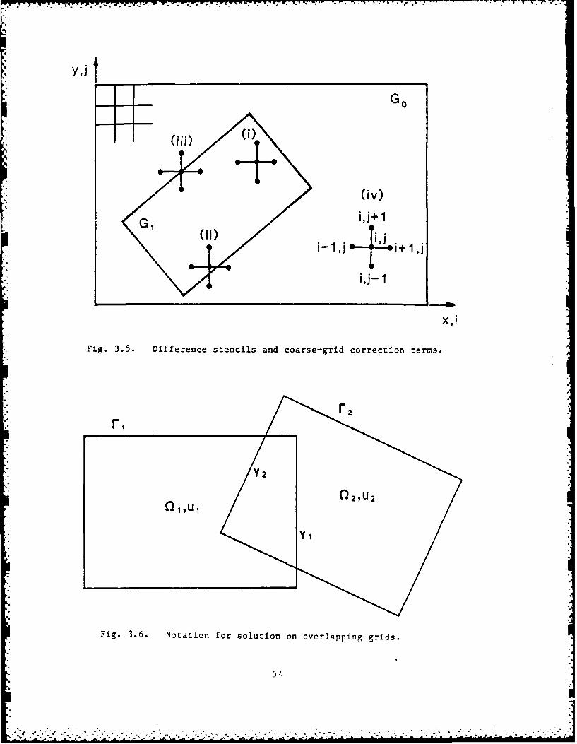
YJ
Go
ql (iv)
ij+l1
i-~ 1, *-" i+ 1,j
i,j-1
X,i
Fig. 3.5. Difference stencils and coarse-grid correction terms.
r2
1,U1 2U
Fig. 3.6. Notation for solution on overlapping grids.
54

1 U 0 ,1j0 + 1)U0 0+1,JO+)
U(10 J0) u( 0-i
Fig. 3.7. Local cell coordinates for bilinear interpolation.
55

' 1 \rr W~fl35CY~qr~.' ".tr ~- u.xwrrwt.wwvw.rJwurvr~r4r..r&.Th -. r; r W~ - -. .*.* -. - -rr~rrr~t-rrr.rr.
'U
I.
I.r
U'
U'I.
3-
56
. - . ..- . . - . - . .U - - 3 U - U U - U - U -

Chapter 4
APPLICATION TO ONE-DIMENSIONAL BOUNDARY-VALUE PROBLEMS
4.1 Introduction
In this chapter, we apply our method to one-dimensional boundary-
value problems. The purpose is to demonstrate the feasibility and
performance of the technique.
The passive adaptive method described in the previous chapter is
applied to the linear, singular perturbation problem:
ey" + a(x)y' + b(x)y - f(x)
(4.1)
Y(Xl) - Yl ; Y(x 2 ) Y2
where e > 0 is a small parameter. Solutions of (4.1) have boundary
and/or internal layers of thickness e in which there is rapid solution
variation. Outside these layers, the solution is smooth. In general,
only boundary layers can exist if a(x) does not change sign on the
interval, 1xl1, x21. If a(x) changes sign, an internal layer can
appear at the turning point, a(x) - 0. (See Bender and Orszag (1978)
for further discussion of the theory of singular perturbation problems.)
Equation (4.1) is a common model problem used to test numerical
methods for the Navier-Stokes equations. With b(x) 0, e is analo-
gous to the viscosity, a(x), to the velocity, and the source term,
f(x), to the pressure gradient.
The passive method is used for (4.1), since the inner and outer
solutions are weakly coupled. For small c, accurate outer solutions
can be constructed analytically by neglecting the second derivative,
dropping one boundary condition and integrating the resulting problem.
The coupling is weak, because the outer solutions can be accurate even
when the boundary layer is completely neglected.
57
- *S'

4-
4.2 Numerical Method
Recall that, in the passive method, the solution outside the re-
finemenL: region is not improved as finer grids are added. Since the
grid gets refined mainly in the boundary layers, we must use a numerical
method that can give accurate results outside of boundary layers when a
coarse mesh is used. As discussed in Section 3.4, only first-order
upwind differencing has this characteristic; it is therefore used for
approximating (4.1).
The first derivative is approximated by one-sided differences:
y(x+ 1 )-y(xj)h if a(xj) > 0
y - (4.2a)y(x 1 ) -yx_ )
if a(x ) < 0h
and the second derivative by central differences:
y(x+ ) - 2y(x ) + y(x i.),- j+ (4.2b)
h2
on a uniform grid, where h - xj+I - xj. The resulting system of
difference equations is tridiagonal and is solved using the Thomas algo-
rithm.
The method (4.2) is used for all grids; the boundary conditions
differ for each.
4.3 Adaptive Procedure
An initial solution is calculated on a base grid. The mesh spacing
on this grid is doubled and another solution calculated using the same
method. The error is then estimated by inserting these two solutions in
(3.7 .3a) with p = 1. Points havinq errors larger than a prescribed
tolerance 6max are flagged, clustered, and fit with refined grids.
* Boundary conditions for new grids are taken from the coarse grid. Solu-
tions are then calculated on each refined grid using (4.2), the error
estimated, and finer-level suhgrids created. The process is repeated
58
........................... ... *.. . . . .

77 7 7*7 7 7- . 7 7
until the maximum estimated error is less than 6max or a minimum mesh
size is achieved on the finest-level grid(s).
The following rules are used to generate a refined grid from a
collection of flagged points:
1. Adjacent flagged points belong to the same refined grid.
2. Flagged points separated by m or less consecutive unflaggedpoints are in the same grid.
3. Grids are buffered with n unflagged points on their bound-aries.
n and m are small integers that are user specified.
Steps 1 and 2 are the nearest-neighbor clustering algorithm in one
dimension. The parameters n and m allow the user some control over
the refined grid sizes; we have used values in the range 1 < n,m < 5.
Note that, in 1-D, refined grid boundaries coincide with parent
grid points; boundary values for fine grids are the parent grid values
at these locations. The mesh size for a subgrid is obtained by dividing
the parent's mesh size by a constant factor, R, the refinement
ratio. An example grid structure after 1 and 2 refinement steps is
shown in Fig. 4.1a & b, where R = 2 and m = n - 1.
4.4 Numerical Results
We illustrate the method by showing the results for a simple bound-
ary layer. Results for more complex boundary layers follow.
Unless otherwise noted, all calculations were made with the follow-
ing parameters:
I. Perturbation parameter, E = 10-2.
2. Maximum allowable estimated error, Smax = 10
3. Maximum number of consecutive unflagged points in a cluster,m = 1.
4. Buffer region equal to one parent mesh length, n = 1.
5. Refinement ratio, R 2.
59

In all plots, adaptive results are indicated by circles, exact solutions
(or very fine grid solutions) are plotted as solid lines.
Example I - Simple Boundary Layer
The first problem has a single boundary layer and is given by:
cy" - y' 0 (4.3)
with boundary conditions:
y(-l) 1 (4 .4 a)
y(1) 2 (4.4b)
This problem has the exact solution:
(e X /e e- l1/e
y(x) - 1 + 2 s ei/) (4.5)YW 2 sinh(1/e)
Figure 4 .2a shows the initial solution calculated on a grid having Ii
mesh points. The outer solution is accurate, even though there are no
points in the boundary layer. For comparison, a solution calculated on
the same grid using second-order central differencing for the first
derivative is shown in Fig. 4.2e.
The error was estimated in the initial solution, and the criteria
indicated the need for a grid spanning 0 < x < t. The boundary con-
dition at x - 0 was taken from the coarse grid solution. The right
boundary condition was (4.4b). The method (4.2) was used to calculate
the solution on this grid; it is shown in Fig. 4.2b.
The error in this solution was estimated, and the third-level grid
spanned 0.4 < x < 1. The solution calculated on this grid is shown in
Fig. 4.2c. As expected, the size of each successive refined grid de-
creases and the boundary layer is better resolved after each adaptation.
The complete adapted solution is given in Fig. 4.2d. The boundary
laver is accurately resolved with an efficient placement of mesh points.
Seven refinement levels were needed; Table 4.1 gives a description of
all grids that were generated.
60

The efficiency of the method can be assessed by comparing its com-
putational work with that of a uniform grid calculation with mesh size
equal to the smallest mesh used in the adaptive method.
We estimate the work for these problems. In adaptive calculations,
the majority of the work is consumed in inverting the tridiagonal sys-
tems. This work is proportional to the number of grid points. We mul-
tiply the cost of the solution on each grid by 1.5 to include the cost
of error estimation and grid genertion. For the uniform grid, we use
only the actual work.
For the simple boundary layer, the uniform grid requires five times
the adaptive grid work for these parameters. Note that this savings
will increase geometrically for similar problems in two and three dimen-
sions.
Example 2 - Two Boundary-Layer Problem
A problem having boundary layers at both endpoints is described by:
ey" - 2xy' + 2y = 0
(4.6)
y(-i) - y(1) = I
The results of an adaptive calculation are shown in Fig. 4.3. The solid
line is a solution calculated using a fine uniform grid. Both boundary
layers are accurately resolved, and the estimated adaptive work is two-
thirds of the uniform grid work.
Example 3 - Internal Boundary-Laver Problem
A problem having an internal boundary layer due to a turning point
is:
Ey" + xy' - 0
(4.7)
Y(-) = 1 ; y(1) = 2The results of the adaptive calculation are plotted in Fig. 4.4 along
with a fine grid solution. Note that the two knees in the solution
receive the most refinement. The region of steep gradient between the
61
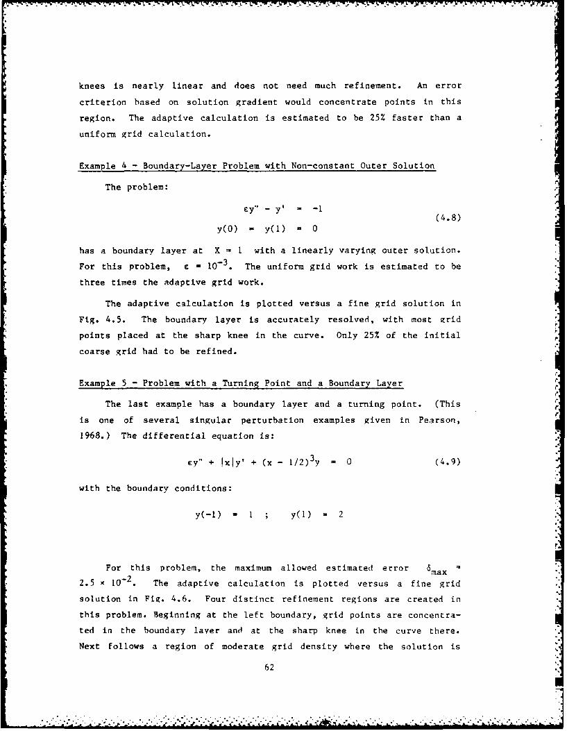
knees is nearly linear and does not need much refinement. An error
criterion based on solution gradient would concentrate points in this
region. The adaptive calculation is estimated to be 25% faster than a
uniform grid calculation.
Example 4 - Boundary-Layer Problem with Non-constant Outer Solution
The problem:
Ey" - y' -1(4.8)
y(O) - y(l) - 0
has a boundary layer at X = 1 with a linearly varying outer solution.
For this problem, e - 10- 3. The uniform grid work is estimated to be
three times the adaptive grid work.
The adaptive calculation is plotted versus a fine grid solution in
Fig. 4.5. The boundary layer is accurately resolved, with most grid
points placed at the sharp knee in the curve. Only 25% of the initial
coarse grid had to be refined.
Example 5 - Problem with a Turning Point and a Boundary Layer
The last example has a boundary layer and a turning point. (This
is one of several singular perturbation examples given in Pearson,
1968.) The differential equation is:
Ey" + jxfy' + (x - 1/2) 3y = 0 (4.9)
with the boundary conditions:
y(-l) = I ; y(1) m 2
For this problem, the maximum allowed estimated error 6,max =
2.5 1-2. The adaptive calculation is plotted versus a fine grid
solution in Fig. 4.6. Four distinct refinement regions are created in
this problem. Beginning at the left boundary, grid points are concentra-
ted in the boundary layer and at the sharp knee in the curve there.
Next follows a region of moderate grid density where the solution is
62
............. ..........................................................................

moderately varying. The grid-point density is also high at the knees
associated with the internal layer. The estimated adaptive work is
approximately. 30% less than that for a uniform grid.
4.5 Conclusions
These examples demonstrate the feasibility of using the passive
solution technique for solving singular perturbation problems. Use of
the upwind difference approximation is crucial to the success of the
method. Figure 4 .2e indicates that, if central differencing had been
used, the whole grid would have been refined.
Estimates of the computational work indicate that the adaptive
method is more efficient than a uniform grid, even allowing for the
additional overhead (primarily error estimation for these prohlems).
No stability or convergence problems associated with adaptation of
the grid were encountered. A smooth distribution of grid points was
generated. Points were concentrated in regions of large curvature;
steep, linear regions were not overrefined.
The Richardson-solution error estimates reliably indicated where
the solution was accurate and where refinement was required, justifying
the expense of computing the solutions used for the estimate.
.
63
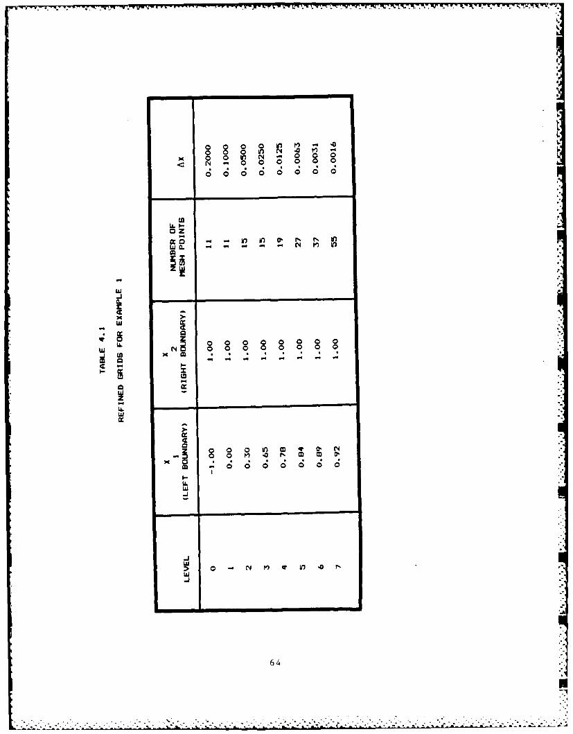
0W Irv 0 ~
o 000
00 U ~ -..
xxLiil
w0 ~ 0 O
ww
- 0 0 v0I' 0. 00 .00 M0 M 00
0-
U-4
w M

(a) 2 level grid structure
I I IT I P I I I f j
(b) 3 level grid structure
Fig. 4.1. Example 1-D grid struccures.
65

-' I I i I I
i° -
I4-
X 02
11
*' - I N.
*I o
TI' I I 1 ' ' 1 I 0)
, , , ,
667
,... ., -. :. ; i ... i. . . Ii

.. . .I I
-.,,
oo
1 0)
I I
° .,- .- 0,
*. l , I r I i .1I I21 I-
', •
,5 -4-4 ""
67

I I I I I I I I
Ii0
~0
- 0 -I
S.d
-4
-4
5-''-4ii!'-I
+10- .J 0
~ru o* II .
a-'9 QJ
-41' I
-4'I-
Sr 0
'-415c-I* I
~ ~. '-40 0 0 0 0 00 0 0 0 0 00 flJ 0
nJ '-I .4 >- -4 .4 -4
68

4-
Ih~.
II I
___________________________________________ -Jj0
H~
0II -
-4I! JI0
Ca
0
A-I0.
LCu
A-I4k -40.I10
xCu
-4
C
I I
0 C C0 C 0 00 W 4. N 0
N .4 .4 .4 .4 .4
69
-*t*.*.*.*.*,.....*...*.*.... .*'**

-II 0
i -0m 0
* •
.- •
1! -Ct I0
* Ci
7* -o

7 1
4
3 0 0
>.~
.-.
71-

00
1*I
0I..
00
110
If I..If
-10
00 -
0 1-
-4xI-
044~
00 0I-u
.4-I0
-40
'S
(V
I
-
1- I I I I jJ
0 0 0 0 0 00 0 0 0 0 00 0 W *. N 0
Al q4
72
-I. I
..- ,. *.***.'4.**......... . . .
4. . - 4. ,,-.-... 4. * . . 4.

'I,
00
0
0
0
4-a000
.0 1
0 0 0
730

- --. -- - .. . A A S
* 0U) 0.
l.A
'I
'-4
* $.0
0 S
-4
".4
N. -4
o -4
*~ 4-.
0
U)'0
- 'K~ I .w 9
0 0 0 0* 0 -~ 0 U)
4., -.4 0 0
A
* 74

Chapter 5
APPLICATION TO A TWO-DIMENSIONAL, LINEAR, CONVECTION-DIFFUSION PROBLEM
5.1 Introduction
In this chapter, we apply our method to the two-dimensional, lin-
ear, convection-diffusion problem:
u x + Voy = E(¢xx + Cyy)(5.1.1)
V (u2 +v2) 1/2
This is another model problem for the Navier-Stokes equations. Because
it is linear and elliptic, it is appropriate for testing our method.
With the addition of source terms, (5.1.1) describes the convection
and diffusion of passive scalars in a flow field. Thus it is connected
with convective heat and mass transfer, which are important in energy-
conversion systems.
Since the problem is two-dimensional, numerical diffusion is
present when the flow is oblique to the grid lines. This error arises
because approximations to derivatives are obtained from one-dimensional
Taylor expansions along coordinate lines. Special methods have been
devised to take account of the local flow angle, e.g., Jameson's rotated
difference scheme (Jameson, 1974) and skew-upwind differencing (Raithby,
1976). We expect our method to align the coordinate system in the re-
fined regions with the flow; special difference procedures should not be
required. Problem (5.1.1) is a useful test of the ability of the method
to accomplish this.
The passive method was used for adaptive solutions of this problem;
justification for using this method was gained from numerical experimen-
tation. However, for a comparison, calculations were also made using
the active method.
75

5.2 Numerical Method
Equation (5.1.1) is nondimensionalized using the magnitude of the
velocity V and a reference length L to obtain:
U'Ox , + V'y, y Pe- 1 (Oxx, + , yy) (5.2.1)
where
L L ' V V
The Peclet number Pe is given by:
VLPe - ____d
To use rotated rectangles, we transform from (x,y) coordinates to
arbitrary rotated coordinates (&,n) related by:
( A() (5.2.2)
where
cose sin eA =
-sine cos 0
and e is the angle of rotation with respect to the base grid. Equa-
tion (5.2.1) transforms to:
UO + -n Pe-(0 + 0nn ) (5.2.3)
where
*Thus the form of the equations is invariant to rotation of the coordi-o..
nate system when the velocities are given with respect to the rotated
coordinates.
76
".i;'': " i i " i Y 1 . . . .
.4. . . . .. . . . .~ .$.,. - \* ** I

- . ly-. - . 7 . W.7 - 7 7- 7
First-order upwind differencing is again used for first deriva-
tives, and second-order central differences for the second derivaties.
The resulting difference equation is:
U + + u-- + v 0+ + + v-8 = Pe- 1(6 + a (5.2.4)
where
= (U + JI) u - 1I)
t i i ,J -ai+,j - ij
i+lj -2Oij + *i-I,jij
with similar expressions for v+ and 6+ . etc.
These difference equations were solved using the Gauss-Seidel
iterative method. The Schwarz alternating procedure (described in
Section 3.6) was used for solving on overlapping grids.
A subroutine was written to solve (5.2.4) on a uniform rectangle.
The solution on every grid was calculated by this routine. Only bound-
ary conditions, step sizes At and An, and the angle of rotation
needed to be supplied. The numerical method and/or the differential
equation can be modified by changing only the solver routine.
5.3 Adaptive Procedure
The adaptive process is similar to that used in the one-dimensional
calculations described in Section 4.3. The primary differences are the
additional procedures required to handle rotated, overlapping rectang-
les.
The nearest-neighbor algorithm is used to cluster the flagged
points, and an ellipse-generated rectangle fit to each cluster. (These
methods are described in Chapter 2.) If some part of a new rectangle
falls outside the problem boundaries, its size is reduced while holding
77
-.. . - .- -. . - -

the angle of rotation fixed. Unenclosed flagged points are then fit
with a boundary-aligned rectangle.
The nominal step sizes on a refined grid are the parent mesh sizes
divided by the refinement ratio R. The actual size is evaluated by
adjusting the nominal step size such that there is an even number of
mesh lengths in each coordinate direction. This is required to calcu-
late 2h solutions. As a result, nominal mesh sizes are usually
adjusted a small amount. The mesh size is adjusted, rather than the
rectangle's size, since the latter may have already been adjusted to
make the rectangle fall within the problem boundaries.
Processing of newly created grids to accommodate the overlapping
grid-solution procedure is required. Grids are first marked to indicate
whether they are isolated or overlap another grid. Overlapping grids
are then sorted into disjoint, overlapping sets. The order in which
,grids are visited in the Schwarz solution procedure is then determined
by recording relative positions of the grids in each disjoint set. The
coordinates of grid-boundary segments that are internal to other grids
are evaluated and stored. This information is used by the Schwarz
driver to update boundary conditions and check for convergence. (The
Schwarz solution process is described in the next section.)
Boundary conditions and initial guesses for fine grids are interpo-
lated from coarse grids using bilinear interpolation (3.8.2). If a fine
grid point lies on the external boundary, exact boundary conditions are
applied. This is important, because interpolation of problem boundary
values from a coarse grid could deteriorate the overall accuracy. Bi-
linear interpolation is also used to update overlapping-grid boundary
conditions during the Schwarz solution process.
An active calculation was also performed by making a small modifi-
cation to the passive program. The adaptive procedure is similar to the
passive method described above, except that, after a new level of grids
has been added, an active solution is calculated using the procedure
described in Section 3.5.
Because the solution error is estimated in the passive program, it
was used as a refinement criterion for the active method, rather than
78

the truncation error, as recommended in Section 3.6. This substitution
is justified for two reasons. First, the active calculation is made
only for a comparison against the passive calculation. Second, in this
problem, the solution error is a good indicator of where the truncation
error is large; the substitution will not have a large effect on the
overall performance of the method. Additionally, the maximum allowed
error in the active calculation was larger than that used in the passive
one.
5.4 Numerical Results
Equation (5.2.1) was solved on the square domain x C (0,10);
y e (0,10), with a constant uniform flow field, and step initial con-
ditions:
u' cose ; v' sin 6
V - ( 7v2 = + (5.4.1)
1 ; Y' > Yo*(O,y') 0 : ;
0 ; Y' < Yo
where 0 is the flow angle with respect to the x-axis. As indicated in
Fig. 5.1, the scalar * diffuses as it is convected downstream.
For large Peclet numbers, diffusion in the streamwise direction
can be neglected. Equation (5.2.1) then becomes the heat equation in
streamline coordinates and an analytical solution can be constructed.
The exact solution *e is:
( /-e (y'-yo0) U' x'v'}IOe(X',y') 0.5 + 0.5 erf (5.4.2)
21/(y'-y o ) v' - x'u'
where yo is the y-coordinate of the step discontinuity at the upstream
boundary x 0.
79
.. .. .. - .. . . .. , --'. -- . .- . . . .. . . -. . . ..- . .. . . . . o . . . . . . - . - . . .. . .
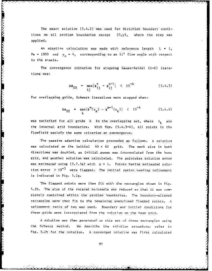
The exact solution (5.4.2) was used for Dirichlet boundary condi-
tions on all problem boundaries except (0,y), where the step was
applied.
An adaptive calculation was made with reference length L = 1,
Pe - 1000 and yo = 4, corresponding to an 1i° flow angle with respect
to the x-axis.
The convergence criterion for stopping Gauss-Seidel (G-S) itera-
tions was:
= maxI& n n-II < 10-4 (5.4.3)GS iij i iJ
For overlapping grids, Schwarz iterations were stopped when:
IOSz - maxI&M(Yk) - M1 Yk)I < 10- 4 (5.4.4)k
was satisfied for all grids k in the overlapping set, where Yk are
the internal grid boundaries. With Eqs. (5.4.3-4), all points in the
flowfield satisfy the same criterion at convergence.
The passive adaptive calculation proceeded as follows. A solution
was calculated on the initial 40 x 40 grid. The mesh size in both
*. directions was doubled, an initial guess was interpolated from the base
grid, and another solution was calculated. The pointwise solution error
was estimated using (3 .7.3a) with p - 1. Points having estimated solu-
tion error > 10- 3 were flagged. The initial region needing refinement
is indicated in Fig. 5.2a.
The flagged points were then fit with the rectangles shown in Fig.
5.2b. The size of the rotated rectangle was reduced so that it was com-
pletely contained within the problem boundaries. The boundary-aligned
rectangles were then fit to the remaining unenclosed flagged points. A
refinement ratio of two was used. Boundary and initial conditions for
these grids were interpolated from the solution on the base grid.
A solution was then generated on this set of three rectangles using
the Schwarz method. We describe the sol,|tion procedure; refer to
Fig. 5.2b for the notation. A converged solution was first calculated
80
................. ................... ..... - . . , .. -......................................
on G1 ,1 " Boundary conditions along the internal boundary Y2 1 were
interpolated from the solution just calculated; then a solution was
calculated on G1 2- Boundary conditions along the internal boundary
Y3 were interpolated from this solution, and a solution was then calcu-
lated on G1 ,3 . This completed a forward sweep.
Boundary conditions along the boundary Y2,3 were interpolated
from the solution on G1,3, and the solution then calculated on G,2.
Finally, conditions along y1 are interpolated from GI, 2 and the
solution calculated on GI. This completed one Schwarz iteration.
This procedure was repeated until the convergence criterion (5.4.4) was
satisfied on all internal boundaries.
The mesh sizes on the three grids were then doubled and another
solution calculated using the Schwarz procedure. (The alternating
method converged in four Schwarz iterations on h grids, and two iter-
ations for 2h grids.) The error was again estimated, and the result-
ing refinement region is indicated in Fig. 5.2c.
In all, three levels of refinement were used. The resulting grids
are indicated in Fig. 5.2d. The size of the refined regions decreases
as more refinement is added, and the central grid tends to align with
the flow. Thus the method "homes in" on the shear layer. Note that the
major source of error is the nonalignment of the upstream boundary grid
with the flow. This error propagates downstream.
Uniform grid calculations were made with meshes finer than the
initial coarse mesh used in the adaptive calculation. The rms solution
errors were evaluated for both adaptive and uniform calculations:1 -1 j - /max jmax - 2
i = 2 i = 2 n5 . .
e '5-5rms (ia-2)(j max2)
where *e is the exact solution (5.4.2). The errors a e plotted vs.
cpu times in Fig. 5.3. (For adaptive calculations, the solution was
interpolated onto the base grid, where the errcr was then evaluated.)
We do not describe the active calculation in any detail here; the
procedure is similar to that described in Section 8.2.3 for the backstep
81
-V

AD-A169 471 ADAPTIVE GRID TECHNIQUES FOR ELLIPTIC FLUID-FLO 2/3PRODLEMS(U) STANFORD UNIV CA CENTER FOR LARGE SCALESCIENTIFIC COMPUTATION S C CARUSO ET AL. DEC 85
IUNCLASSIFIED CLRSSIC-95-19 N11114-82-K-6335 F/O 26/4 NL

%
ii
1.8 '1.
.911111.2 - L1 _4 Il
MICRO~COPY RESOLU TION TEST CHART
NA' DNA, B-FA, IT.AOS - 96S-
%p

problem, except for the refinement criterion. For this calculation, the
maximum allowed error was 5 x 10- 2 (compared to 10- 3 for the passive
calculation). The calculation was made with two levels of refinement,
and the generated rectangles were smaller in size, compared to the
rectangles at the same level in the passive calculation. This is a
consequence of using a larger error criterion. The rms errors in the
active solution were also calculated and are plotted in Fig. 5.3.
Figure 5.3 illustrates that both adaptive methods are considerably
more efficient than uniform grid calculations. For fixed cost, the
adaptive error is smaller or, alternatively, for fixed error, the
adaptive calculation costs less. For example, for an accuracy of
3.5 x 10- 2 (as indicated in the figure), the passive method runs
approximately 15 times faster than the uniform-grid calculation. The
trend of the passive curve indicates that its advantage increases as
higher accuracy is required.
For a single level of refinement, the active calculation is found
to be somewhat more efficient than the passive one--a result of the less
conservative error criterion in the active method. However, there is a
crossover in performance for two levels of refinement; the passive
method becomes more efficient. The crossover occurs because the active
method exrends additional work updating the outer solutions, which do
not need to be updated. For high levels of accuracy, the passive method
is more efficient for this problem.
5.5 Conclusions
These calculations have shown that the passive method applied to
the linear convection-diffusion equation is accurate and efficient when
compared to uniform fine-grid calculations. The adaptive overhead (cal-
culation of 2h solutions, error estimation, and grid generation) is
included in the cost. The advantage of the adaptive method increases as
higher accuracy is required.
Refined rectangles are automatically aligned with the flowfield,
thereby minimizing numerical diffusion. Linear interpolation of bound-
ary conditions was found to provide sufficient accuracy. The use of
upwind differencing was important for providing accuracy outside the
shear layer and also for reliable grid-refinement information.
82

..
0.99
* - 0.01
Fig. 5.1. Schematic of linear convection-diffusion problem.
83
" .w " " " n'' .' ' .. . ... . . . . . . . . . . . . . .J.

S1,2
y 2,
84

Fig. 5.2(c). First-level refinement region.
Ist ~ lee irid2n lee grids- I3 leve grids
Fig.5.2(). esuling efied gids
-~85
V a

10-1
0
Mw 10-2
I0\
* uniform
0 passive
x active
10-3100 13 200 103
NORMALIZED CPU TIME
Fig. 5.3. Adaptive vs. uniform grid performance.
86

Chapter 6
NUMERICAL SOLUTION OF THE NAVIER-STOKES EQUATIONS
As mentioned previously, our main interest is flows described by
the steady, laminar or Reynolds-averaged, incompressible Navier-Stokes
equations. In this chapter we present the governing differential equa-
tions and the numerical methods used to solve these equations. These
methods will be embedded in the adaptive method.
6.1 Navier-Stokes Equations
6.1.1 The Incompressible Navier-Stokes Equations
For completeness, we present the unsteady equations, which are
incompletely parabolic. The steady equations are elliptic and are
obtained by dropping the time derivatives.
In Cartesian tensor notation, the time-dependent, incompressible,
Navier-Stokes (momentum) equations are:
a u+ --. (6.1.1)
at ax p axxi ax ax
where ui(x.,t) is the local fluid velocity, p is the density, p is
the pressure, and v the viscosity. The continuity equation solved in
conjunction with (6.1.1) is:
ou - 0 (6.1.2)
which requires the velocity field to be divergence-free.
The Navier-Stokes equations can be nondimensionalized in the fol-
lowing way. Using L and V as reference length and velocity scales,
respectively, the dimensionless variables,
X" i xi/L
U, U u/V
87
. - .
p- p/pV2
T = t/(L/V)
are substituted into (6.1.1) and after rearranging obtain:
S+ - 2P- + Re-' (6.1.3)ax ax - + axJ ii xj
" where Re is the Reynolds number, Re = VL/v.
Equation (6.1.3) governs both laminar and turbulent flows. How-
ever, at large enough Reynolds numbers (the exact value depending on the
geometry), the flow becomes turbulent and is no longer steady.
Turbulent flows are difficult to compute because of their unstead-
iness and because they possess a wide range of relevant physical scales.
Accurate resolution of these scales requires using a prohibitively large
number of grid points, even for moderate Reynolds numbers. Conse-
quentlv, the direct solution of (6.1.1) for turbulent flows requires
supercomputers and is restricted to relatively low Reynolds numbers.
Such calculations are referred to as direct or full simulations (see,
e.g., Ferziger, 1983).
6.1.2 Reynolds-Averaged Eauations
Although turbulent flows are unsteady, time-averaged quantities
(velocity, pressure, etc.) can be defined. To derive the averaged equa-
tions for these quantities, the velocity is decomposed into a mean and
fluctuating part:
= u + ut (6.1.4)
where ui and ui denote the mean and fluctuating velocities, respec-
tively, and u' = 0. The pressure is similarly decomposed. Substitut-iing this decomosition into (6.1.1) and (6.1.2) and time-averaging
results in the Reynolds-averaged Navier-Stokes equations yields
- -- 2--a au a2u au'ui I i 7t j
t + + V (6.1.5)p ax ax ax ax
j i j j j
88
"'' -" -' * . . .. . . . . . . . . . . . . ..'-- - - -" -'" "- -', "'' ' - -"..... . . *. *,'i - ,.f " . .

and an averaged continuity equation (.
La . 0 (6.1.6)
rThese equations describe the mean flow field W and pressure 7, which
are steady if au/at = 0.
The term - puhue is called the Reynolds stress, and it represents
the influence the turbulence exerts on the mean flow. Auxiliary
equations must be supplied for the Reynolds stress in order to solve
(6.1.5) and (6.1.6)
An eddy (or turbulent) viscosity relationship is a common constitu-
tive equation for the Reynolds stress. It has the form:
Su~ auulut v - (6.1.7)i J T~ (ax +ax
where a relation for VT, the turbulent viscosity, must be specified.
Equation (6.1.5) can be nondimensionalized in the same manner as
Eq. (6.1.1). The resulting equation is similar to (6.1.3), except that
the Reynolds number is replaced by an "effective" Reynolds number:
Reef f VL
eff
where v eff = VT + v"
If the eddy-viscosity model is used, the laminar and averaged equa-
tions have the same form and therefore are similar from a computational
standpoint. The major difference is that VT varies spatially and is-1 -1
generally much larger than v. Consequently, Reef f >> Re- . This dis-
tinction is important, because the difficulty of computing these flows
varies inversely with the effective Reynolds number.
6.1.3 Eddy-Viscosity Models
To complete our discussion of the turbulence equations, we briefly
discuss some models for vT . A more detailed discussion of these models
can be found in Rodi (1980) or the earlier review of Reynolds (197b).
)" 89
"..1

The simplest expression for vT is the zero-equation model:
VT - t [I -'i+ + - /2 (6.1.8)T xi a xi axI)
where c is a constant and Z is a given length scale.
A more complex relation for vT is the one-equation model:
VT f ck /2 Z (6.1.9)
where k -, -u is the turbulent kinetic energy and is described by a2 ii
transport equation similar to (6.1.11) below. c and Z have the same
meaning as in (6.1.8).
In the popular two-equation k-e model,
VT - ck2 /c (6.1.10)
where e represents the dissipation of turbulent energy. c is a con-
stant; k and e are governed by transport equations of the form:
3tx k a /T V kt I P- (6.1.11)
at ax ax ak axjJ k i.
+ = + P -C 2- (6.1.12)at x ax a ax IC k E
where ak, GO, Cej, CE2 are constants and P is the production
aui
Note the similarity between the laminar equation (6.1.1), Reynolds-
averaged equation (6.1.5), and the k and C transport equations
(6.1.11) and (6.1.12). All of them can be written in the following
general form, for the steady case:
= a jr + S (6.1.13)ax1 ax ax~
90
-7.

Equation (6.1.13) is elliptic, and the same numerical methods can be
applied to all the equations. Our adaptive technique has been applied
only to the steady, laminar equations. However, by modifying the flow
solver, it can be extended to apply to the averaged turbulent equations,
including any of the various eddy-viscosity models discussed above.
6.1.4 Steady, 2-D, Laminar Equations
Our adaptive procedure was applied to the 2-D, steady, laminar,
incompressible eauations. In Cartesian coordinates, the dimensionless
x-momentum equation is:
a -1 au 2ua + auv = Re 2 + Re- (6.1.14a)ax 3y ax ax2 ay2/
The y-momentum equation is:
auv av 2 L+Re-/2 2I -i + v v (6.1.14b)ax ay ayax2 a2
The continuity equation is:
aU + v ,, 0 (6.1.16)ax ay
This set is complete, but there is no explicit relationship for the
pressure.
An equation for p can be derived by taking the divergence of
(6.1.14) and using continuity to simplify. To derive this equation,
first rewrite the momentum equations (6.1.14) as:
= Mx (6.1.16a)ax
p My (6.1.16b)av
adding 3/ax (6 .1.16a) to a/V3y (6.1.16b) results in a Poisson
enuation for the pressure:
91
............................... .
: ' ' " " : - " - -" " " - - ' " -: : ; : ,:: :; : ::.:-,. ::: : . ,-:i. : :: : . :., .:, . f. .--ii_

-_ (6.1.17)ax2 ay2 ax ay p
The source term, S can be simplified using continuity, giving:
__2 2 \/_\ay2 - + axa auapx ) y( T2y (6.1.18)
Equations (6.1.14) with (6.1.17) are an alternative description of in-
compressible flows.
Equations (6.1.14)-(6.1.15) are invariant under rotation, and con-
sequently so is (6.t.17). These equations are therefore directly appli-
cable to arbitrarily rotated grids.
6.2 Staggered Grid
The Navier-Stokes equations are solved on a uniform, rectangular,
staggered grid (first proposed by Harlow and Welch, 1965). On this
grid, each dependent variable is defined at a different set of loca-
tions, as indicated in Fig. 6.1. Pressure nodes are located at the cell
centers, u, the x-component of velocity at the midpoints of the hori-
zontal sides, and v, the y-component of velocity at the midpoints of
the vertical sides.
This grid can be viewed as a composite of three grids, one for each
variable. For example, u1 , vii, and pi1 are all located at
different points, as shown in Fig. 6.1.
For incompressible flows, the staggered grid has some important
advantages over a nonstaggered grid (on which all dependent variables
are defined at the same locations). As seen in Fig. 6.1b, the staggered
grid has no pressure nodes located on its boundaries. Consequently, the
pressure does not have to be explicitly specified there; this is not the
case for a nonstaggered grid. This is an advantage, since boundary
conditions for the pressure are not normally known. A Neumann boiindarv
condition for pressure is implicitly contained in the numerical method,
as discussed below.
The staggered grid is also more accurate than ' nonstaggered grid,
as the finite differences are taken over shorter diqtances. They are
92
-M -- ss- i~-.A 1 ~ ~ ~ . .- .--

therefore more accurate than centered differences on a nonstaggered grid
(see Fig. 6.2).
Furthermore, on a nonstaggered grid, only every second pressure
node is coupled (see Fig. 6.2b). As a result, an oscillating or check-
erboard pressure solution is oossible (see discussion on pp. 115-117,
Patankar, 1980). This cannot occur on a staggered grid.
A disadvantage of the staggered grid is that the boundary cells are
different from the normal cells, as indicated in Fig. 6.1b. Careful
treatment is required to maintain accuracy at these points (se- Section
6.3.2).
6.3 Finite Differences
In this section, we present the finite difference approximations
used for the mmentum equations. The treatment of the pressure equation
is given in Section 6.4 below.
Standard methods for solving differential equations approximate
derivatives by finite differences (FD) constructed from local Taylor
expansions. An alternative technique is the finite volume (FV) method,
which approximates the integrated conservation equations. We use the
latter.
We demonstrate the application of the FV method to the x-momentum
equation (6.1.1 4 a); the y-momentum equation is handled in a similar
manner.
Consider the finite volume centered abound ui, shown in Fig. 6.3.
Equation (6.1.14a) is integrated over this volume; the volume integrals
are converted to surface integrals using the divergence theorem, and the
line integrals are evaluated using the mean-value theorem. The result
is an exact integral-conservation equation given in terms of face-
average values, designated e, w, n, and s (east, west, etc.):
K2 u + p Re1 a i lPew e - w ax e axA
u v - axe a xw, (6.3.1)
- . = (uv ay n ay,
93

= -Y
Equation (6.3.1) represents the conservation of u-momentum in the finite
volume (momentum theorem).
Next, the average face fluxes are approximated in terms of the
neighboring grid-point values. The formula used to define the face
values detemines the resulting difference approximations; these are
discussed next.
6.3.1 Pressure Difference
The pressure gradient is the simplest term to deal with, since the
pressure grid points are located at the centers of the cell faces, as
noted in Fig. 6.3. This results in the equivalent centered, second-
order FD approximation:
dlx Lp Pi+,j -Pij (6.3.2)ax i+1/2,J 6x Ax
6.3.2 Diffusion Terms
For the diffusive fluxes, second-order central differences are also
used, e.g.,
au__I i u__ - uia
au _du -uii~ -u( 6.3.3a).yln y 6 " n Ay
au_ Sul uii - ui- (6.3.3b)ays
Subtracting (6.3.3b) from (6.3.3a) and dividing the result by Ay gives
the second-order central difference for the second derivative:
2 u - 2u +6 u ij+1 i + u ij- 1 (6.3. 3c)
6y 2ij (Y
As noted in the previous section, the staggered grid is nonuniform at
horizontal boundaries for the u-grid; consequently, (6.3.3) has to he
modified for boundary cells (refer to Fig. 6.4). A common approximation
at the lower boundary is:
94
: ,t * , .. .", " " "
" -" ' : l " . ..." " "-" S"I " : " I -
" " " " " " i u

Su , i / i2 o (6.3.4)
Subtracting (6.3.4) from (6.3.3a) and dividing by Ay gives the fol-2u
lowing approximation for y2ayi,l
2 Y 2 u - 3 u32 u I2ui° - 3u'l + ui,2 (6.3.5)ay i,l (Ay 2
However, the acccuracy of this approximation is 0(1); i.e., it is not
consistent with the differential equation. Since a 2u/ay2 is large
near solid walls, it is important to approximate this term accurately.
A better approach is to use the first-order-accurate approximation:
3 2 u 2u i'o - 3u i'l + u 1,4i2 3 (6.3.6)
a yi'4 ()2
or the second-order approximation:
a2 u 16u - 25u i + lou - u
6 i o , i 2 - i 3 ( 6 .3 .7 )
To test these approximations, a fully developed channel-flow problem was
calculated. This problem has the exact solution:
u = y(l-y)
v 0 (6.3.8)
0 < x < 0 <y< i
Using either (6.3.6) or (6.3.7), the converged numerical solution agrees
with the exact solution. Using the approximation (6.3.5), significant
solution error results near the grid boundaries. We use the first-order
scheme (6.3.6) in most of our calculations.
95
12,!

6.3.3 Convective Terms
First, we briefly review the problems associated with approximating
the convective terms. Our discussion is directed toward steady flows,
although similar difficulties are encountered in time-dependent prob-
lems.
Central differencing (CD) of the convective term has two associated
difficulties. First, at large Reynolds numbers, CD may produce solu-
tions that have large spatial oscillations or "wiggles". An illustra-
tion of this in one dimension was given in Fig. 4 .2e.
It can be shown (see, e.g., pp. 24-26, Peyret and Taylor, 1983)
that, if CD is used to solve the one-dimensional, linear, convection-
diffusion equation,
- v 2 ; u,v const. (6.3.8)x x2ax
oscillations in the solution will occur unless
Re I Ax < 2 (6.3.9)
ReAx is called the cell Reynolds number. This restriction may require
using prohibitively fine meshes for large Reynolds numbers.
Even though (6.3.9) is strictly valid only for (6.3.8), this re-
striction is often applied to the momentum equations, which are non-
linear, multidimensional, and have source terms. However, one cannot
prove that (6.3.9) must be satisfied for CD to give smooth solutions to
the momentum equations.
We have found smooth solutions to the laminar back-step problem
using CD for cell Reynolds numbers as high as 150 (see Chapter 8). Kim
and Momn (1985) have found similar results. The apparent difficulty is
that streamwise diffusion is not important in this flow. For further
discussion, see Ferziger (1986).
The second difficulty with CD is that instability may occur when
iterative methods such as Causs-Seidel are used to solve the system of
difference equations. If the difference equations are written in matrix
form:
96
|* .- . - ** *.a - .* * * * *!.- *.:.A..'*.

ttAu - b (6.3.10)
then a sufficient condition for convergence of the Gauss-Seidel method
L is that A be diagonally dominant, i.e.,
imaxJai > F • i = max (6.3.11)
j.1
where aij are the elements of A. (This criterion also holds for many
other iterative methods.) CD applied to (6.3.8) or the momentum equa-
tions gives diagonally dominant matrices only if ReAx < 2.
The possibility of obtaining spatial oscillations and the instabil-
ity of iterative methods have led researchers to search for alternative
differencing approximations. Upwind differencing (UD) was the first
remedy tried. UD always gives diagonally dominant matrices and smooth
solutions; however, it introduces excessive numerical diffusion, as
discussed below. The search for better methods remains an active re-
search area.
We discuss the schemes which we use next.
Central Differencing
Second-order central differencing for the convective terms is equi-
valent to assuming that u is piecewise linear between the four neigh-
boring points of uij. On a uniform grid, this means that face fluxes
are averages of the adjacent grid-point values. For example, the for-
mulas for the horizontal fluxes in (6.3.1) are:
2 /uij + uij) 2j
u = 2' ) (6.3.12a)e 2
22 (uij ui-
u 2 )(6.3.12b)w 2
For the vertical fluxes, v must be averaged, i.e.,
u v uij 2uii+l)vi+ 2 v J (6.3.13)
97

p _D .. .. - .... .s : °" ~ r * [ * . % R. .
.- - . . . . .. -- ".° - • - .
0*
Upwind Differencing
In upwind differencing, the fluxes at the cell faces are taken from
the "upwind" grid point values. The "wind direction" is determined by
the sign of the velocity at the cell center.
For the horizontal fluxes, the sign of u determines the wind
direction, e.g.,
2 2U U le ij f
u w ui-l,j
(6.3.14)
2 2ue u i+1,
j
2 2 u ij < 0
u -uw ij
The sign of v at the cell center determines the wind direction for the
vertical fluxes. This value, v, is found by averaging, e.g.,
v - (vI [ + + v1 1 1 + vi+11... ) (6.3.15)
The vertical fluxes are then obtained from
u = (6.3.16a)n
ul+I,J v < 0
v v 2i i+lj (6.3.16b)
n -2
and similarly for uS and vS.
UD is first-order accurate, but, more importantly, the leading term
of the truncation error is Droportional to the second derivative. For
positive uij, an upwind approximation to u(3u/3x) on a regular (non-
staggered) grid has the following truncation error:
98
4;, -: >.iKX >& i. . . . ..... ..

* -.. ... .
uui - U Ax I2 + O(Ax2 (6.3.17)
u ij Ujj Ax 2 2
The truncation error thus introduces numerical diffusion. At even mod-
erate Reynolds numbers, the numerical diffusion can greatly exceed the
physical diffusion. Consequently, if the grid is not sufficiently
refined, the result may be an inaccurate, overly diffused solution.
Hybrid Differencing
The next two methods are composites of central and upwind differ-
encing. The first scheme, attributed to Spalding (1972), uses central
differencing at a grid point if the magnitude of the local cell Reynolds
number, ReAx < 2, and upwind differencing otherwise. (For two-
dimensional problems, Rey - 'v is used as the criterion for the y-
derivatives.) Additionally, where ReAx > 2, the (physical) diffusion
term in (6.3.1) is discarded to partially offset the numerical diffusion
introduced by the upwind differencing.
This scheme has the stability and monotonicity of the pure upwind
method. However, in most practical computations, ReAX >> 2 in most of
the flow. Consequently, this method is only marginally better than pure
UD.
The second hybrid scheme is Patankar's power-law method (Patankar,
1980, and 1981). It is based on the exact solution to (6.3.8) and is
similar to the exponential scheme of Allen and Southwell (1955).
Face values are found in the following manner. Equation (6.3.8) is
integrated along the line xL < x < xR, with the boundary conditions
4 (xL) = -
(6.3.18)
to give:
-L exp(e(x-x L)/Ax) - I- (6.3.19)
R L exp(e) -1
where
99
V.i

uAxRe - -
V
Ax x xR - xL
Equation (6.3.19) is used to evaluate the velocities at the cell faces.
For example, using
¢(x i = uii
(X i+I) =Ui+l,j
the face velocity ue is found by evaluating (6.3.19) at x - xi+1/2,
with u taken as the average of uij and ui+,j at the previous time
step or iteration.
Patankar uses a power-law fit to the exponential (6.3.19) that is
cheaper to evaluate. The velocities for all cell faces are evaluated in
the same manner and substituted in the integral equation (6.3.1).
Patankar's method is stable for all cell Reynolds numbers. It is ap-
propriate for approximating (6.3.8); however, its accuracy when applied
to the momentum equations is not clear.
The power-law scheme is similar to Spalding's hybrid method, but it
has a gradual transition from central to upwind differencing in the
vicinity of ReAx = 2.
QUICK Differencing
The last method discussed is the upwind-biased, QUICK difference
scheme (Leonard, 1979a,b). (QUICK is an acronym for Quadratic Upstream
Interpolation for Convective Kinematics.) Face fluxes are determined by
quadratically Interpolating the solution from the two adjacent, upwind
grid points and the one adjacent downwind point at each face.
For the horizontal fluxes, the resulting approximation is (Shyv,
1985):
100
.. . . . . . . . . . . . . .

3 2 2 72 1 2- - U
2 2 +l 'ij1 8 i-~ + -9 i2, lije w 1 2 + 7 2 3 2 2
ui+2,, 8Ui+l, j Cui, + )i- ; < 0- -~j -- uii i
(6.3.20)
The vertical fluxes are found in a similar manner.
Dividing (6.3.20) by Ax gives a second-order-accurate, noncen-
tered FD for the convective term Bu2/ax. the overall method remains
second-order accurate as second-order approximations are also applied to
the diffusion terms.
QUICK's accuracy is comparable to central differencing and more
accurate than the upwind or hybrid schemes (Leschziner, 1980, Leschziner
and Rodi, 1981, Durst and Pereira, 1983). However, the method does not
always give diagonally dominant matrices, and convergence is not guar-
anteed (Han et al., 1981). QUICK can also give oscillatory solutions,
although they are generally smoother than those obtained with CD. Our
experience confirms these observations (see Chapter 8).
6.4 SIMPLER Solution Technique
Patankar's SIMPLER (Semi-Implicit Method for Pressure-Linked Equa-
tions Revised) method is used to solve the systems of finite difference
approximations to the momentum and Poisson equations. The method is
described in Patankar (1980); we give a summary and an alternative in-
terpretation of the scheme in this section.
The procedure is iterative. Beginning with an initial velocity
field, which does not necessarily satisfy continuity, we do the follow-
ing:
1. Calculate the pressure by approximately solving a Poisson equa-tion (6.4.2).
2. Approximately solve the linearized momentum equations (6.4.3)for velocity, using the pressure from Step 1.
3. Calculate the pressure correction by approximately solving aPoisson equation (6.4.7). (The pressure correction is formula-ted to make the updated velocity in Step 4 satisfy continuity.)
101
4. Calculate the velocity correction (6.4.6) and add it to thevelocity from Step 2. (The velocity correction is proportionalto the gradient of the pressure correction.)
5. Check for convergence:
max n+l n
Steps 1-5 are cyclically repeated. As the solution converges, the di-
vergence of the velocity field, the pressure correction, and the veloc-
ity correction are all driven towards zero. The final velocity and
pressure fields satisfy the discretized momentum and Poisson equations,
respectively, to within a convergence criterion.
The equations solved in Steps 1-3 are linear systems and are ap-
proximately solved at each step using the same iterative solution
method. We describe this method in Section 6.4.4 below.
The SIMPLER technique was heuristically formulated. However,
Patankar does not clearly indicate what forms of the differential equa-
tions are being approximated (e.g., the type of linearization for the
momentum equations, the specific form of the Poisson equation, etc.).
to clarify this, we next present an alternative interpretation of the
method.
6.4.1 Pressure Calculation
In Step 1, the pressure is evaluated from an approximation to the
Poisson equation (6.1.17). The source term is evaluated by first cal-
culating the right-hand sides of (6.1.16a,b) using the current veloci-
ties u and v For example,
Mx - j 6uv - 2( du 6u (6.4.1)ij x6x 2 ij
Mx is evaluated at all u-grid points, My at all v-grid points (see
Fig. 6.5).
The divergence of M - [Mx, My]T and the Laplacian of p are both
evaluated using second-order central differences, resulting in a Poisson
equation for the pressure:
102
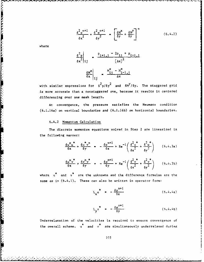
L27. Ili LaVI -C 7-o
dx ] (6.4.2)
whe re
62P p'1+1.1 2p + p 11I'
6x 2ij (Ax)2
6MX MX M
6x I - Ax
with similar expressions for 6 2 p/6Y 2 and 6Mg/6y. The staggered grid
is more accurate than a nonstaggered one, because it results in centered
differencing over one mesh length.
At convergence, the pressure satisfies the Neumann condition
(6.1.16a) on vertical boundaries and (6.1.16b) on horizontal boundaries.
6.4.2 Momentum Calculation
The discrete momentum equations solved in Step 2 are linearized in
the following manner:
6u n u6Su 6Tn (6.4.3a)
6x dy 6x 6x2 6Y2/
n1 2* 2v*+u~ v + +Re 1 v d (6.4.3b)-Tx 6yx 2 d 2 /
where u and v *are the unknowns and the difference formulas are the
same as in (6.4.1). These can also be written in operator form:
L u 6= - A... (6.4.4a)x 6x
* n+ 1L v =-(6.4.4b)y 6y
Underrelaxation of the velocities is required to ensure convergence of
the overall scheme. u *and v* are simultaneously underrelaxed during
103

the approximate solution of (6.4.3); the procedure is described in Sec-tion 6.4.4 below.
6.4.3 Velocity and Pressure Corrections
In Step 4, the velocity corrections u' and v' are added to the
velocities calculated in (6.4.3) to give the updated velocities:
n+1 Uu u+u
(6.4.5)Vn + l
=' V i+V
The corrections are formulated to make the updated velocity field sat-
isfy continuity.
The velocity corrections are related to the pressure correction
p' by eliminating all of the contributions from the velocities at the
neighboring points in the momentum equations (6.4.3) to give:
u' -A u '
6x
(6.4.6)V ' A Av AL
'
dy
where Au and Vv depend on the difference scheme.
A similar correction is made in Chorin's projection method (Chorin,
1968). There, the pressure is used instead of p', and the velocity
correction is interpreted as an operator that projects an arbitrary* u~n+l p
velocity field, u , onto a divergence-free field, . p' plays a
similar role in SIMPLER.
The equation for p' is found by requiring that un+ 1 satisfy
continuity. Inserting (6.4.5) with (6.4.6) into a discretized version
of continuity (6.1.2) results in the following Poisson equation for p:
621, + =- uIA v/A(6.4.7)6x 6y 6x + S4
The same differencing is used for (6.4.7) as for (6.4.2).
If the velocity is prescribed on the houndaries, the boundary
condition for (6.4.7) is o' 0. Intermediate values of un+ 1 will
104
not satisfy continuity, because (6.4.7) is only approximately solved.
At convergence, un 1 = - u continuity is satisfied and p'
vanishes everywhere.
6.4.4 Solution of the Linear Systems
An iterative method is used to solve the linear systems (6.4.2-3)
and (6.4.7) in Steps 1-3. The scheme is essentially an ADI method; it
is called a "line-by-line" method by some authors. One iteration con-
sists of making line Gauss-Seidel relaxations in one coordinate direc-
tion, followed by similar relaxations in the other direction.
For example, the solution at points along a vertical line (indica-
ted by the dots in Fig. 6.6) are simultaneously evaluated using the
current neighboring solution values (at locations indicated by the
x's). The equations for the dotted variables are tridiagonal and are
solved via the Thomas algorithm. Lines are solved in succession in one
direction, then in the other direction.
Since the SIMPLER scheme is iterative, it is not necessary to solve
the linear systems exactly at each step. We perform one line-by-line
iteration of each system for each SIMPLER iteration. Sweeps are made in
the flow direction to get the best convergence rate.
As noted above, u and v are underrelaxed simultaneously when
(6.4.3a,b) are solved using the line-by-line method. Next, we describe
how the underrelaxation is performed.
The difference equation (one row of (6.4.4a)) for the velocity u
at some grid point P can be written:
au E an + f (6.4.8)p p nbnp
where the subscript nb denotes the neighboring grid points of P; the
summation is to be taken over all neighboring points.
Equation (6.4.8) can be rewritten as:
S n a nbunb +f nu u +- u (6.4.9)
4"p p a pPi
105
nnwhere u is the velocity from the previous SIMPLER iteration. The
term in the brackets can be regarded as the change in up for the
current iteration.
To reduce this change, an underrelaxation factor, w, where 0 < w
< I is introduced:
u = un + W -abub un (6.4.10)
p p a
Equation (6.4.10) can be rewritten:
au* * (W-1) n-a u Z a u +f+- a u (6.4.11)W p nb nb W p p
The relaxation is introduced by scaling the diagonal terms ap and add-
ing the last term in (6.4.11) to the right-hand side of (6.4.4) before
performing the line-hy-line iteration.
The relaxation factor must be determined experimentally; we have
used w - 0.85, as recomended by Zebib (1984) for most calculations.
However, at higher Re and smaller grid sizes, w must be reduced to
keep the SIMPLER method from diverging.
6.5 Implementation of Central Differencing for Rex > 2
As discussed in Section 6.3.3, central differencing (CD) can de-
stabilize the solution method when ReAx > 2. The matrix equations
representing the x- and y-momentum equations are not diagonally dominant
when ReAX and Rey > 2, respectively. Without diagonal dominance,
the line-by-line method becomes unstable, and the solution blows up.
A stable method can he constructed using the defect-correction
method (see. e.g., Stetter, 1978, Hemker, 1981, Auzinger and Stetter,
1982), which we describe below. Note that this method does not elimi-
nate oscillations in the solution. Oscillations are artifacts of the
difference entiations, not the solution method.
Assume that we wish to solve the differential equation:
Lu = f
106
f,

Denote Lh as a difference method that gives diagonally dominant matri-
ces, and Lh as a more accurate method, which does not necessarily give
diagonally dominant matrices. A solution can be computed that satisfies
L2Lh by means of the following iterative procedure:
LIu ° 0 = f (6.5.1a)h
1 u n - f+ (LhIu n Lh2un) (6.5.1b)
An iterative method can be used to approximately solve the linear system
(6.5.1b) at any intermediate step, e.g., one line-by-line sweep. How-
ever, at convergence, the solution satisfies:
2nu -f (6.5.2)
We apply the correction procedure (6.5.1) to the x- and y-momentum equa-
tions (6.4.4a,b) in the following manner:
n+1 2L"u - -1----+ (LIu n - L 2) (6.5.3a)
x 6x x x
L1v + (L Ivn _ L ) (6.5.3b)y ay ~ y y
where Li and LI represent Patankar's hybrid scheme and L2 and2 x y a
L are central differencing. The Poisson equation for pressure (6.4.2)yis unchanged. The solution method is stable for all cell Reynolds num-
bers, and the converged solution is second-order accurate.
Any other difference method can be easily substituted into an
existing program. One need only insert the correction (LI un -Lun )
on the right-hand side of the equation as a source term.
107
,... - ... --.. -.- --i -- .i -. . - . i -i .. - . .. .. . . .- . - . .. .-- i . .- .- ,- i.-- -

6.6 Numerical Conservation
The notion that numerical approximations to the fluid-flow equa-
tions should satisfy integral conservation equations to within round-off
errors is an important and controversial one. In this section, we
briefly review the concept and how it applies to single grid computa-
tions. We discuss the implications for local adaptive refinement in the
next chapter.
We begin by defining numerical conservation. A scheme is said to
be conservative if it satisfies a discrete version of the Gauss diver-
gence theorem. For example, consider the continuity equation in vector
form:V * u = 0 (6.6.1)
Integrating (6.6.1) over a volume V, and making use of the divergence
theorem allows us to write:
fV.udV = 5 f.nds (6.6.2)V
where S is the surface of the volume and n the outward unit-normal
to the surface.
Assume that we have the following difference scheme for (6.6.1):
Vh.u = 0 (6.6.3)
A discrete analog of the divergence theorm in 2-D is:
Z w I ( V AxAy = E wij unAS (6.6.4)
(interior points) (boundary points)
where un is the velocity normal to the boundaries, and wI and w2
are weighting functions dependent on the numerical integration formulas.
The scheme (6.6.3) conserves mass if (6.6.4) is satisfied exactly to
within round-off error.
The quadrature method should be an inverse of the difference method
(analogous to the integral and differential operators). The weightinq
functions w1 and w2 are usually taken to be unity, which corresponds
to the trapezoidal rule or the mid-point rule, depending on whether the
108

integrated quantity is located at cell faces or cell centers, respec-
tively. For w1 = =w2 1, the difference equations (6.6.3) are summed
over all grid points.
If the scheme conserves mass, all interior grid-point velocity
differences cancel, and the remaining boundary terms can be rearranged
to represent the surface integral in (b.6.4). Since velocity differ-
ences cancel, there are no numerical sources or sinks of mass in the
interior of the domain.
A similar analysis can be made for the momentum equations. If all
discrete volume integrals can be reduced to surface integrals, the
scheme conserves momentum.
The construction of conservative schemes is simplified with the
finite volume method, if the conservation form (6.1.1) of the differ-
ential equations is used as a starting point. (In the nonconservation
form, the convective terms are written as uj(aui/axj).) If face-flux
expressions are formulated such that the flux across a common face of
adjacent control volumes is the same for both control volumes, then they
will cancel when summed over interior grid points.
The integral fluid-flow equations are conservation statements for
the various physical quantities: mass, momentum, energy, etc. The dis-
crete integrals are not, in general, equal to their respective analyt-
ical counterparts. However, the quantities may be exactly conserved in
a numerical scheme. Conservation and accuracy are separate issues. An
accurate, nonconservative method will give the exact solution (including
conservation) in the limit of vanishing mesh size, and consequently he
conservative in the limit if the differential equation is conservative.
There has been considerahle debate over whether methods need to he
conservative or not. For shock calculations, it is well known that a
conservative method can be used to compute the correct shock speed and
strength. Instability has been attributed to a lack of conservation in
some time-dependent schemes for viscous flows. However, there are also
instances where a nonconservative method gave more accurate results than
a conservative one. (Roache, 1982, pp. 32-33, reviews the early liter-
ature on this subject.) The consensus is that conservative methods
shouild be used whenever possible.
109
• o o -. . . . . . . . . . . . . . . . .... . . . . . ... . . .. -

p -
On a staggered grid, central differencing for all terms in the
momentum eauations conserves mass and momentum--and kinetic energy in
the limit of infinite Reynolds numbers (Zabusky and Deem, 1971). But
the scheme is conservative only if approximations similar to (6.3.4) are
used for the diffusion term for boundary cells. The more accurate
schemes (6.3.6) and (6.3.7) which we use make the method nonconserva-
tive.
We make one final point. Given a conservative method, it is
necessary that the surface integral in (6.6.4) vanish for steady flows,
if global conservation is to be maintained. For rectangular grids, this
means that the normal velocities at all boundary grid points must sum to
zero. We therefore took care to specify boundary conditions for the
base-grid computations such that global continuity is satisfied.
In this chapter, we have described the solution techniques used for
the steady, laminar equations. These methods are incorporated in our
general flow solver, which is applicable to an arbitrarily rotated, uni-
form rectangle. This solver is used to calculate h and 2h solutions
for the base grid and any refined grid in an adaptive computation.
110
- ' " . - , ', - 7 : - f "
- .." • " - - - - . . " . . - , .- ,- .-
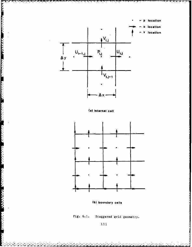
- p location
-O - u location*t - v location
S l- 1,j P ,j Uldj
Il,j-
Ay-
(a) Internal cell
* N
--- m -±- -
(b) boundary cells
Fig. 6.1. Staggered grid geometry.
111

dP )~FR-1/ 2 P 1 1/ 2
dx iAx
u p
(a) staggered grid
x2A x 1+1 2Ax
UIP U,P UP U,P
I-i 1.11+2
(b) nonstaggered grid
Fig. 6.2. Centered differences on staggered and nonstaggered grids.
112

* Uiji. i
V1.1 Vi+1 .j
I nI
e I A
'aj 11.11,-I Ii i
ig 6.. Fnt ouefr u
Fig6. . 6.3.rnc Fintenvolum for b udr. cls
S11

ij+ 1
M Y
Pi j I-1.
9ij I
Fi 6.X 5. FiieMoum or p
I __
Fig. 6.5 L inb-ie volutior met. d
- - 1-

Chapter 7
ADAPTIVE NAVIER-STOKES SOLVER
In this chapter we describe the procedure for adaptively solving
the steady, laminar, Navier-Stokes equations. We begin by summarizing
the adaptive process, then follow with detais of the active solution
method, boundary conditions and conservation, and, finally, error-
estimation method.
7.1 Summary of Adaptive Process
The adaptive method will be applied to the laminar backward-facing-
step problem in Chapter 8. Because it is a strongly coupled problem,
the active method is required. All refined grids are specified a priori
to be boundary-aligned; rotated grids are not used. Finally, the re-
fined grid boundaries are restricted to be colinear with parent grid
lines, as indicated in Fig. 7.1.
Although our method is not restricted to nonrotated refinement, two
factors influenced this choice. The primary factor is a consequence of
the backstep geometry; use of rotated rectangles would decrease the
adaptive efficiency. This is Justified in Section 8.2.3. A secondary
factor is the difficulty of conservatively interpolating boundary condi-
tions for rotated grids; this is further discussed in Section 7.3.
With the exception of the solution method (active) and nonrotated
refinement, the adaptive procedure is similar to that used for the
linear convection-diffusion problem in Chapter 5. We summarize the
adaptive solution process next, then discuss implementation details in
the sections that follow.
The base-grid solution is calculated first. All velocity boundary
conditions are Dirichlet, except at the outflow boundaries, where zero
derivative conditions are applied. A solution on a doubled mesh is cal-
culated with the same boundary cnditions and used to estimate the trun-
cation error via the procedure discussed in Section 3.7. Points having
estimated truncation errors larger than a specified value are clustered;
cluster(s) are fit with boundary-aligned, refined rectangle(s).
115

Boundary conditions for refined grids are all Dirichlet. Exact
values are used wherever grid points lie on the problem boundary. For
fine grid boundaries interior to the problem domain, values are inter-
polated from the parent grid using a procedure that conserves mass
across the boundary (see Section 7.2 below). Initial guesses are
hilinear interpolations from the parent grid.
An active solution is then calculated on the two-level grid system
according to the algorithm outlined in Section 3.5. A solution is first
calculated on the fine grid(s). Correction terms for the coarse grid
are then evaluted and a solution recalculated on the coarse grid. Iter-
ation between coarse and fine grids is repeated until internal fine-grid
boundary values no longer change.
Because the method is iterative, the solution on each grid level is
not reauired to be fully converged at intermediate steps. (The same
approach is used with the momentum and Poisson equations in the SIMPLER
method-see Section 6.4.4.) Rather, the solution may be iterated a
fixed number of times (similar to multigrid methods) or to a given level
of partial convergence, before switching grids. The iteration strategy
is discussed in Chapter 8.
After the two-level solution has converged, its error is estimated
by doubling the mesh sizes for all grids, and solving. The truncation
error estimate is computed over the whole domain. Since the region of
large truncation error decreases in size after each adaptation, the new
level of refined grids is normally contained within those of the pre-
vious level.
7.2 Implementation of the Active Solution Method
We show how the active solution method is implemented for the lan-
inar equations by applying it to the two-grid system shown in Fig. 7.2.
Extension to more levels is straightforward.
We use the notation of Section 3.5. At convergence, the solution
on the coarse grid G0 in region Q, should agree with the fine-grid
solution. The solution consists of the velocity components 11 and v
and the pressure p. However, as p can be determined from u and v,
116
7 " i- l'
:' " " - ."
i • " '.°, . . ,-' " o
°. . , .' .' ."
J " i

%7*- . . w IV L , K V
we require only that u and v agree on G0 and G1 on Ql" As
discussed in Section 3.5, uH = uh on Q, is enforced by calculating
correction terms for the coarse grid.
If m indicates the active outer iteration number and n the
SIMPLER (inner) iteration number, the correction terms are computed by
modifying the right-hand sides of the coarse-grid momentum equations
(6.5.3) in the following manner:
L1 n+l fn I mLx,HUH = -C (-x x + a xL x,Hu h (7.2.1a)
yIVn+1 (1-a) fn + ayL1 , v m (7.2.1b)
yH H y y y y,H h (..b
where
f n + _L+ 1 n L2 un)
x 6x (Lx ,HUH x,HUH
f n p+ + LI vn L L2 n)y 6y yLy,HVH y HV )
f af(,Y
a (x,y), a (x,y) all if (x,y) C nY0 if (x,y) 1
Note that the defect corrections are contained in f and fy. (Recall
that they are used to implement central differencing for the convective
terms, as discussed in Section 6.5.) The parent grid-masking arrays a
and ay are initialized to zero and are modified when an offspring (re-
fined grid) is created. On the finest grids, ax . ay = 0 everywhere.
The correction terms in (7.2.1) are evaluated by interpolatingfine-grid solution values and using them in the coarse-grid operator L.
according to the rules given in Section 3.5. Although uh and v sat-
2 1isfy the more accurate Lh operator on the fine grid, LH must be used
for the corrections in order to give at convergence:
uH = uh where ax I
117
.. . ....... . . . . . . . .
*- , .- , L ~ w., -,x-wx- 1 -w- *,. ; .V . .. . -o . .- V YWV
vH V h where ay 1
This can be verified hy multiplying (7 .2.1a) with x= I by the in-
verse of LI and doing similarly for (7.2.1b).
7.3 Treatment of Boundary Conditions
Boundary conditions for refined grids are interpolated from coarse-
grid solutions using a procedure that conserves mass. Additionallv,
when new grids are created, certain coarse-grid boundary conditions may
require modification to maintain global continuity. In this section, we
describe boundary conditions and discuss conservation and interpolation
issues related to rotated grids.
7.3.1 Interpolation of Fine-Grid Boundary Conditions
As previously discussed, bilinear interpolation is normally used to
transfer solution values between coarse and fine grids. However, inter-
polation can destroy numerical conservation at internal fine-grid bound-
aries.
Consider the west face of the central coarse-grid control volume in
Fig. 7.1. The location of coarse-grid velocities are indicated by
solid-head arrows, fine-grid velocities by open-head arrows. The fine
grid is denoted by the dashed lines; the refinement ratio is 2. Since
the fluid density is constant, the mass flux through the west face is
Proportional to the integral of the velocity over the face.
To conserve mass, the coarse-grid and fine-grid mass fluxes across
the west face should be exactly equal. If the mid-point rule is used
for integration, the coarse-grid mass flux is equal to the coarse-grid
normal vel',city at the face. The fine-grid mass flux is the sum of the
two fine-grid velocities on the face.
If fine-grid velocities are linearly interpolated from the coarse
grid, mass will not generally be conserved. However, linearly inter-
nolating the coarse-grid velocity from the fine grid exactly conserves
mass. Thus, linear interpolation from fine to coarse grids conserves
mass, while coarse to fine interpolation does not. To be consistent,
118
?I...... .

St- - .- .- - IftM. 'W -, *., ..- - - -
the coarse to fine interpolation should be the inverse of the fine to
coarse grid procedure.
Such a procedure was suggested by Berger (198 4a), and is similar to
methods used in TVD schemes for hyperbolic conservation laws (see, e.g.,
Van Leer, 1979). In this method, the normal velocity is assumed to vary
linearly on the coarse-grid cell boundary, as indicated in Fig. 7.3.
The slope is taken as the slope of the line connecting the two adjacent
coarse-grid point values, as indicated in Fig. 7.3. Fine-grid normal
velocities are determined by this line.
In other words, fine-grid normal velocities, uih(x), are obtained
from:
-H(XH -H xj H)ih(X) L H (x -x) + uH(x) (7.3.1)
for
Xj -h < x < xj + h
Tangential velocities on internal boundaries are bilinearly interpolated
from coarse grids; this does not affect the mass balance on the control
volume.
An equation similar to (7.3.1) is used to interpolate v on hori-
zontal faces (e.g., north and south faces in Fig. 7.1); u is hilin-
early interpolated on these faces.
This scheme conserves only mass at the internal grid boundaries.
It would be difficult to construct a method that also conserves addi-
tional quantities, e.g., momentum, kinetic energy, etc.; the necessity
for osing such a method is not clear. As shown in the next chapter, the
scheme we use provides good accuracy and gives no stability problems
when applied to the backstep flow.
7.3.2 Modification of Coarse-Grid Boundary Conditions
As mentioned previously, exact boundary conditions are applied if a
fine-grid hotindarv lies on the nroblem boundary. There are also coarse-
irid points on these "coincident" boundaries. If exact boundary values
119
. - .,

are applied on all grid points on a coincident boundary, the numerical
integral of the normal velocity on the boundary will be different on
each grid; i.e., mass will not be conserved. To be conservative, all
integrated mass fluxes should be equivalent.
Coincident boundaries are handled in the following manner. Exact
values are applied on the finest grid, giving the most accurate approx-
imation to the integrated mass flux. To maintain conservation, boundary
values for coarse-prii points on a coincident boundary are linearly
interpolated from the next finest grid.
In practice, when a new level of refined grids is created, boundary
conditions are specified. At coincident boundaries, values for the next
coarsest grid are obtained by linear interpolation from the fine grid;
i.e., they are changed from their previous values. This is repeated for
still coarser grids.
By using the conservative, coarse-to-fine-grid interpolation scheme
(described in the previous section) and modifying coarse-grid boundary
conditions at coincident boundaries, mass is conserved on the multilevel
grid system.
7.3.3 Interpolation and Conservation for Rotated Grids
In this section, we discuss conservation and interpolation for
rotated grids; further discussion can be found in Berger (1984b). From
Fig. 7 .4a, it is clear that conservative interpolation is complicated by
the rotation. While an interpolation scheme that conserves mass is pos-
sible, the construction of a scheme that conserves additional quantities
is more difficult. We shall therefore consider mass-conservinv schemes.
Note that the schemes used with "patched" "r zonal grids cannot be
used for rotated grids. Adjacent patched qrids do not overlap; rather,
their boundaries interface along a common line. The interpolation is
one-dimensional and therefore simpler compared to two-dimensional inter-
polation required for rotated, overlapping grids. See Hessenius and Rai
(1984) or Rai (1985) for a discussion of interpolation methods used for
patched grids.
120

Several interpolation approaches for rotated grids are possible; we
outline a straightforward one. Consider interpolation of fine-grid
boundary values along the line a-a shown in Fig. 7.4b. The mass flux
normal to the line a-a, m , can be obtained from a mass balance ona-a
the triangular region, using the coarse-grid velocities uH and vH.
Assuming velocities are piecewise constant on cell faces gives:
S - wH (g+2h) = (fu + Hv H) (7.3.2)
where (g+2h), f and H are the lengths of the triangle's sides.
m is then to be distributed to the fine boundary grid cellsa-a
#1, 2, 3 lying along line a-a, i.e.,
m =m + m + m(7.)a-a 1 2 3 (7.3.3)
If the flux is distributed according to individual cell areas, then
= .h *1 21 M 2 (g+2h)m a-a h h
and
- "(7.3.5)3 (g+2h) a-a
The fine-grid velocities u and uh are obtained from (7.3.4). ;3
is added to the flux obtained for the balance of cell #3, calculated
using a similar procedure.
Coarse-to-fine grid interpolation could be performed in a similar
manner. However, the calculation and distribution of mass fluxeq
depends on the assumed velocity variation on cell faces and on tne
nuadrature method used to integrate the mass along the boundaries. (The
midpoint rule is implicit in the procedure outlined above.) It may be
possible to use arbitrary variations (e.g., constant, linear, quadratic, r
etc.) and integration methods, although this is not clear.
Fuchs (1985) ,ises a simpler approach. He solves the steadv, lami-
nar equations on two overlapping rectangular grids (similar to those
shown in Fig. 3.6) with a multigrid method. For each grid, internal
121
- ,. . 2

boundary values are linearly interpolated from the other. Interpolated
values are then "corrected" such that global continuity is satisfied on
the respective grid. Fuchs does not indicate how the values are correc-
ted; presumably they are either scaled or a small correction is added to
each such that global continuity is satisfied. Fuchs notes that the
corrections are second-order in magnitude. The computed results are
only qualitatively evaluated (streamlines are plotted); however, the
author concludes that the interpolation scheme works adequately.
As noted in Section 6.6, whether a method should be strictly con-
servative or not is a debated issue. We made calculations using non-
conservative, bilinear interpolation for internal fine-grid boundary
conditions and other calculations on single grids in which global
continuity was not satisfied. The nonconservative calculations con-
verged slower (on the order of 10-15%) and also were somewhat less
accurate compared to similar conservative computations, but no stability
problems were encountered with the nonconservative schemes.
7.4 Error Estimation
In this section, we describe the error-estimation 2ethod used forthe steady, laminar equations.
Assume that an active solution has been calculated on a multilevel
grid system. Let uh and vh represent this solution on all grid
levels (h should be regarded as the finest mesh size). The meshes are
doubled on all grids, and an initial guess for each is obtained by in-
terpolating from its respective h-grid. An active solution U2h and
V21-0 is then calculated.
For each grid, the truncation error estimate is calculated only at
points not contained in finer-level grids. For example, for the grids
shown in Fig. 7.2, the estimate is calculated at all points on G, and
only at those points not in the region Q, on Go .
The solution error estimate is calculated first. For example, the
error in uh is found by computing:
122
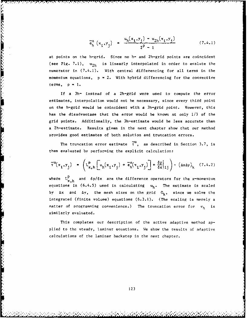
ehUt) u h(Xi'Yj) - U2h(Xi'yj) (7.4.1)2 p -
1
at points on the h-grid. Since no h- and 2h-grid points are coincident
(see Fig. 7.1), u2h is linearly interpolated in order to evalute the
numerator in (7.4.1). With central differencing for all terms in the
momentum equations, p = 2. With hybrid differencing for the convective
terms, p - 1.
If a 3h- instead of a 2h-grid were used to compute the error
estimates, interpolation would not be necessary, since every third point
on the h-grid would be coincident with a 3h-grid point. However, this
has the disadvantage that the error would be known at only 1/3 of the
grid points. Additionally, the 3h-estimate would be less accurate than
a 2h-estimate. Results given in the next chapter show that our method
provides good estimates of both solution and truncation errors.
'UThe truncation error estimate r , as described in Section 3.7, is
then evaluated by performing the explicit calculation:
(xy) L (LPh L y + • Axi Ak (7.4.2)
where Lp and 6p/6x are the difference operators for the x-momentumx,h
equations in (6.4.5) used in calculating uh. The estimate is scaled
by Ax and Ay, the mesh sizes on the grid Gk, since we solve the
integrated (finite volume) equations (6.3.1). (The scaling is merely a
matter of programming convenience.) The truncation error for vh is
similarly evaluated.
This completes our description of the active adaptive method ap-
plied to the steady, laminar equations. We show the results of adaptive
calculations of the laminar backstep in the next chapter.
123
................ ..-

/I. Carse grid
w
-4-al-
X -* u,v coarse grid
.~ u,v fine grid
Fig. 7.1. Boundary-aligned refined-grid geometry.
124
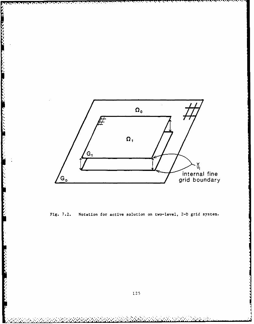
Go internal finegrid boundary
Fig. 7.2. Notation for active solution on two-level, 2-D grid system.
125

17 1
X coarse grid velocity0 Interpolated fine grid
velocity
* NormalVelocity
coarse grid cell B
X1 -H X jH X
Fig. 7.3. Conservative coarse-to-fine grid interpolation.
126

Section A
(a)
Section A
/f
27

128

Chapter 8
APPLICATION TO THE LAMINAR BACKSTEP
In this chapter, we present the results of adaptive computations of
laminar flow over a backward-facing step. We first describe the physi-
cal flow and the corresponding computational model. The results of
uniform grid calculations and a justification for using nonrotated
refinement are then given. Next, results of preliminary adaptive grid
calculations are presented. A performance evaluation at a single Rey-
nolds number follows. Finally, we show results of adaptive calculations
over a range of Reynolds numbers.
8.1 Description of the Problem
The flow through a straight channel having a sudden asymmetric
expansion is called the backward-facing step problem (see Fig. 8.1a).
Separated flows resulting from such changes in geometry are common in
energy conversion devices; the device's performance often depends on the
structure of the flow in these regions. As a result, the backstep prob-
lem has received considerable experimental and theoretical attention.
In this section, we discuss the experimental flow which we shall simu-
late.
8.1.1 Experiment of Armaly et al.
Armaly et al. (1983) studied the flow through a two-dimensional
sudden expansion, having an expansion ratio of 1:1.94. The test section
had a long, straight inlet channel to provide a uniform inlet flow.
Similarly, the exit channel was long to allow a fully developed velocity
profile to develop.
Experiments were conducted over a range of Reynolds number covering
the laminar, transitional, and turbulent flow regimes; we discuss only
the laminar results. Streamwise velocity profiles were recorded, pri-
marily in the section downstream of the backstep. The reattachment
length, XR, was measured as a function of the Reynolds number. Pre-
diction of this parameter is difficult and is therefore used to check
the accuracy of a numerical method.
129
C..- :.j. ; j~~.j?

The measured reattachment length is plotted in Figure 8.19 for
*Reynolds numbers, 50 < Re < 600. The Reynolds number is defined:
uhRe - n
V
where um is the maximum inlet velocity, h is the step height, and v
the kinematic viscosity. The flow is laminar in the range 50 < Re <
900. Above Re = 900, the flow begins to undergo transition prior to
reattachment. At still higher Reynolds numbers, the entire flow becomes
turbulent.
The streamwise velocity in the inlet channel at the sudden expan-
sion was measured and found to be "close to that of a fully developed
channel flow, with a slight deviation from a parabolic profile." The
normal velocity at this location was not measured. Fully developed con-
ditions were found to occur in the outlet channel; the location moved
downstream with increasing Reynolds number.
Cross-channel measurements were made to determine the two-
dimensionality of the flow. The flow in the plane of the sudden
- expansion was found to be two-dimensional. The flow in the channel
* downstream of the step was also two-dimensional at low Reynolds numbers,
* but became three-dimensional for Re > 300, with 3-D effects increasing
with Re. Additionally, an elongated recirculation bubble annears on
the top wall for Re > 300. The location and length of this bubble is
also a function of the Reynolds number.
Because the geometry is simple, the boundary conditions well-
defined, and the data available, this flow is useful for evaluating the
accuracy of a numerical method. We describe our computational model of
this flow next.
8.1.2 Computational Model
The flow is simulated on a rectangular domain, using a uniform
base grid shown in Fig. R.lh. (The mesh size may he different in the
two coordinate directions.) An expansion ratio of 1:2 is used so that
the step-corner lies on a mesh point. The box length is fixed in the
y-direction; the x-direction length, XL, was variable. It was taken
130
. . -...... .. . . . . . . . . . . . . . . . .. . ., .7 - -

A. o --. . . . . '. .. . o . . . . ---4 .-. -• . . . . . . - r _ _
to be four times the experimental reattachment length, as recommended by
Armaly et al.
A parabolic streamwise velocity profile and zero normal velocity
are specified at the inlet. Along all walls, both velocity components
are zero. Fully developed velocity conditions, au/3x = av/ax = 0 are
used at the outlet, x = xL.
Note that two approximations are made in the model. First, the
modeled expansion ratio is 3% larger than the experimental one. To a
first approximation, computed reattachment lengths should be - 3% larger
than the experimental values. Calculations were made by Zebib and Homsy
(1984) on nonuniform grids using both expansion ratios. Their results
confirm that the reattachment length is proportional to the step height.
The second approximation concerns the inlet velocity. Because the
experimental streamwise velocity had a slight deviation from a fully
developed profile, a small, nonzero normal velocity is expected in the
plane of the expansion. Use of zero normal velocity in the computation
will cause the computed reattachment lengths to deviate from experimen-
tal values, hut the effect should be small. A better approach is to use
an L-shaped computational domain and specify fully developed channel
conditions farther upstream in the inlet channel.
As a result of these approximations, computed reattachment lengths
should agree with the experimental data to within 10%, for Reynolds
numbers for which the flow is two-dimensional, i.e., for Re < 300.
8.2 Uniform Grid Calculations
During the development of the adaptive program, uniform grid cal-
culations were made for testing and debugging the basic solver. We als-
experimented with three convective-difference schemes and evaluated the
error estimation procedure on uniform grids. In this section, we pre-
sent results taken from these studies.
All calculations presented in this chapter were made on a VAX
11/780 in double precision.
131
%

r.
8.2.1 Velocity Profiles
All adaptive calculations were made in the range 100 < Re < 600.
For these Reynolds numbers, all flowfields display similar behavior.
Velocity profiles for Re 1 100 with xL/h - 12 are shown to illus-
trate the qualitative nature of the flow; the calculations are not
described in detail. Quantitative results are given in sections that
follow.
Figure 8.2 shows two surface views of u, the x-component of vel-
ocity. (These plots are somewhat distorted; the actual aspect ratio
(y:x) of the domain is 1:6.) u varies smoothly from the parabolic
" profile to another fully developed profile at the outlet. The region of
* negative u behind the step indicates the recirculating region. Reat-
tachment occurs where u changes sign along the bottom wall. For this
calculation, xR/h - 3.6. In the latter half of the channel, streamwise
gradients are small.
Figure 8.3 gives v, the y-component of velocity; it has rapid
variation near the sudden expansion. Downstream of the inlet, v is
negative in the shear layer. Farther downstream, v drops towards
zero. Immediately behind the step, v is positive in the recirculating
region. The maximum magnitude of v is approximately 10% of the maxi-
mum magnitude of u.
Greater detail can be seen in Figs. 8.4 and 8.5, where u has been
plotted along lines of constant y/h and x/h, respectively. The
behavior of u near the bottom wall is seen in Fig. 8.4a. The smooth
behavior of u in the vicinity of the step is shown in Figs. 8.4b-e.
These figures also show the smallness of the streamwise gradients far-
ther downstream. Specification of fully developed conditions at the
outlet is consistent; no abrupt changes occur near this boundary.
Figure 8.5a shows the variation of u with y in a plane passing
through the the recirculation region. In Fig. 8.5b, the u-profile just
downstream of reattachment is plotted. Figures 8.5c,d show that u i
nearly parabolic downstream; a reference parabola is included in these
figures.
132

In Fig. 8.6, v is plotted at constant y/h locations. Figures
8.6b-d illustrate the rapid variation of v just downstream of the
step. As discussed in Section 8.2.3 below, this region has the largest
truncation error and thus requires the most grid refinement. Figure 8.7
illustrates the y-variation for v, which becomes more gradual as the
flow moves downstream.
8.2.2 Comparison of Convective Difference Schemes
For Re - 100, mesh-refinement studies were made using central
(CD) and Patankar's power law (HY) differencing schemes for the con-
vective terms. (Both schemes are described in Section 6.3.) Table 8.1
summarizes the important parameters for the calculations. Initial
guesses for each case were bootstrapped from the previous case.
Table 8.1 shows how the number of iterations for convergence de-
pends on the total number of grid points; both schemes converged in
approximately the same number of iterations, except for Case 4. Nor-
malized cpu times were 0.007 and 0.009 sec/iteration/cell for HY and CD,
respectively. The difference in costs is due to the calculation of the
defect-corrections in the CD scheme (see Section 7.2). On a per itera-
tion basis, the CD scheme is slightly more expensive, although, as dis-
cussed below, the payoff in accuracy is substantial.
The Case 5 CD calculation converges in relatively few iterations,
because its solution is not very different from the Case 4 solution from
which it was bootstrapped. From this near mesh independence, we conclu-
ded that the 192 x 128 CD calculation is a good approximation to the
exact solution. The calculated xR for this grid is approximately 10%
larger than the experimental value, as expected (see Section 8.1.2).
Figures 8.8 and 8.9 are typical plots that illustrate the accuracy
and convergence of the solution as the mesh size is decreased. They
show that, on the same mesh, the CD solution error is significantly
smaller than that for HY, and the CD error decreases faster as the mesh
is refined.
Taking the 192 x 128 CD result as a good approximation to the
exact solution, the rms solution errors were calculated for all other
cases. These errors are tabulated in Table 8.2.
133

-."
The errors for the 96 64 CD case are larger than expected. There
are two causes for this. First, they are not accurate, as they are
comparable in magnitude to the iteration-convergence criterion, 10- 4 .
Secondly, when the criterion is reduced to 10 , the errors on the
96 64 grid become approximately one-half of the respective errors on
the 48 32 grid; the method becomes first-order accurate (see discus-
sion below). Since the 96 64 and 192 128 solutions are nearly
identical, we conclude that the error in the 96 64 solution is negli-
gible at interior grid points and that the significant error is caused
by first-order approximations, similar to (6.3.6) used at boundary cells
(see section 6.3.2).
The errors are also plotted in Fig. 8.10. These plots also indi-
cate the accuracy and convergence properties of the two methods. The
order of accuracy of the method ("p" in Eq. (3.7.1)) is the slope of
the log plot. We find that HY is first order (p - 1), CD second
order (p - 2) as expected.
To summarize, we have shown that central differencing for the con-
vective terms is more accurate than Patankar's power-law scheme. The
added expense of its implementation (through the defect-correction
method) is small, and the correction procedure does not degrade the
overall convergence rate of the method.
As indicated in Table 8.1, central difference solutions were cal-
culated for cell Reynolds numbers as high as 100. No stability problems
were encountered and no wiggles were found in solutions; clearly, the
commonly applied condition, Re < 2, is too restrictive.
Only a few calculations were made using the QUICK scheme (described
in Section 6.3). One calculation was made at Re = 100, using the Case
2 grid in Table 8.1. The method converged in 76 iterations, giving
X R/h - 3.85 similar to the CD calculation, and the rms errors were
somewhat smaller. The cpu time was 0.009 sec/iteration/cell. For this
* case, the performance of QUICK is comparable to CD.
Two QUICK calculations were made at Re = 600. The first was on a
42 16 grid with XL/h - 42. Convergence was achieved in 900 itera-
tions, and oscillations were present in the resulting solution. A sec-
ond calculation was attempted on an 84 16 grid, with the same xL/h.
134
V[.
However, after 1000 iterations, the run was aborted, since the solution
was converging very slowly. This can be compared with a 420 x 20 CD
calculation at the same Re, that converged in 1400 iterations. Be-
cause of the slow convergence at high Re, QUICK was dropped from
consideration. (klthough it was not tried, QUICK implemented by the
defect-correction scheme may converge faster.)
Due to its accuracy, stable implementation, and wiggle-free solu-
tions at large Re, central differencing was selected for use in all
adaptive calculations presented in Secti(:ns 8.4 and 8.5 below.
8.2.3 Exact vs. Estimated Errors
Uniform grid calculations were also msde to test and evaluate the
error-estimation method. In this section, wo show the results of cal-
culations made at Re = 100, using central differencing.
Calculations were made using 24 x 16 and 12 x 8 grids. The so-
lutions were inserted into (7.4.1), with p = 2 to give the u-solution
error estimate; the v-error estimate was similarly computed. To
evaluate the accuracy of the estimates, the exact solution error
(uh - uexact) was computed using the 192 x 128 central difference
solution as the "exact" solution.
Absolute values of the errors are plotted in both contour and sur-
face views. When considering these figures, recall that the actual
aspect ratio (y:x) for the rectangles is 1:6; in the plots, the
ratio appears to he 1:1.5. The surface views provide a perspective of
the errors. The plotted values have been normalized by the maximum mag-
nitude so the differences in the elevations are exaggerated.
The estimated and exact solution errors for u and v are given
in Figs. R.1 and 8.12, respectively. The plots show that the topog-
raphy of the exact error is well represented by the estimate, especially
when the coarseness of the grid is considered. Away from the step, the
estimated magnitudes are relatively accurate, and are generally high.
For example, the location and magnitude of the maximum error in u is
predicted well. The heights of the humps in the v-error are similarly
well predicted. Overestimation of the error is preferable to underes-
timation.
135
a ~ ~ ~ ~ 7 7-tM~fA L..

Near the corner, the error estimate is inaccurate because the
higher-order terms in the expansion (3.7.1) are large. Because the h-
and 2h-solutions differ considerably in this region, the error is poorly
predicted. The accuracy of the estimate improves on finer grids.
The truncation error estimate is computed by substituting the solu-
tion and its solution error estimate into (7.4.2). The exact truncation
error is evaluated by substituting the 192 x 128 central difference
solution into the difference operator in (7.4.2).
The truncation error for u and v are plotted respectively in
Figs. 8.13 and 8.14. As discussed in Section 3.7, these estimates are
not expected to be as accurate as the solution error estimates. Al-
though there is less similarity between exact and estimated topographies
for these errors, the estimates do indicate where the truncation error
is large and, thus, where grid refinement is required. Truncation error
also is generally overpredicted. These plots illustrate the "noisy"
behavior of the truncation error. Smoothing of the estimates is re-
quired if they are to be used in a global refinement method.
These results indicate that the Richardson error procedure provides
reasonably accurate estimates of the solution and truncation errors,
even on coarse grids.
Before closing this section, two final points are discussed. We
first discuss the relationship between solution error and truncation
er:or and some of the implications. We then give a justification for
using nonrotated grid refinement.
Consider the contour plots of the errors for both u and v,
Figs. 8.11-8.14. The figures illustrate how the truncation error is
convected and diffused through the flowfield, resulting in the solution
error, as discussed in Section 3.7. Since the truncation error has a
long-range influence on the solution error, the active solution method
is used for adaptive computations of this flow. The truncation error
shows that refinement is required primarily in the vicinity of the
sudden expansion.
These error plots provide a justification for using nonrotated re-
fined grids. The refinement region defined by the truncation error
136
"4 ' 4"---"- -" - " .- *".-.-...-.> .- -.- > ' . . - . .- -.. . .- - ... . . . . ..* . . .. . . .*

estimates for u and v encloses most of the upstream portion of the
base grid.
Preliminary adaptive calculations showed that a single rectangle
with a small angle of rotation (< 10* relative to the x-axis) is gen-
erated, with its corners falling outside of the problem domain, as
indicated in Fig. 8.15a. The rectangle would have to be reduced in size
and unenclosed bad points fit with overlapping boundary-aligned grids,
similar to the procedure described in Chapter 5. The rectangles that
would result from this procedure are sketched in Fig. 8.15b.
The cost of generating the solution would increase due the work
required for solving on overlapping grids at each level. Since the
rotation is small, this added cost is not expected to outweigh the
benefit of reduced "rotational error". As a consequence of this, and
also due to the difficulty of constructing a conservative 2-D interpo-
lation scheme, we elected to use boundary-aligned grid refinement for
the backstep problem.
8.3 Preliminary Adaptive Calculations at Re - 100
Preliminary adaptive calculations were made during the development
and testing of the program; results of these studies are presented in
this section. A notation for the grids is first given, followed by
results of studies that investigated the convergence properties and
iteration strategy for the active solution method. (The active solution
procedure is described in detail for a typical calculation in Section
8.3.2.) Finally, results are given to illustrate the influence that the
location of "fictitious" internal, fine-grid boundaries has on the solu-
tion accuracy.
All calculations in this section were made at Re - 100. Since the
calculations were only preliminary, Patankar's power-law convective dif-
ference scheme was used; central differencing is expected to give simi-
lar results.
137

8.3.1 Notation for Refined Grids
In the adaptive calculations described in the remainder of this
chapter, the geometry of all grids is similar. In this section, a
simplified notation for the grids is defined.
Refined grids are boundary-aligned, as discussed in Section
8.2.3. Each base or refined grid, Gk covers a rectangular domain:
x e (0,XL) ; y c (0,2) as indicated in Fig. 8.16. The coordinates
(x,y) are normalized by the step height, h. Grids are described using
the notation:
Gk: Nx x Ny ; XL
where N and N are the number of cells in the x- and y-directions,X yrespectively. The domain of Gk is denoted "k"
The internal, fine-grid boundary for a refined grid lies along the
line (XLk, 0 < y < 2) and is denoted Yk"
8.3.2 Convergence of the Active Solution Method
A calculation was made using a two-level grid system to investigate
the convergence properties of the active solution method. The
parameters for this calculation are:
Go: 12 x 8;XL - 120 xL 0
Gi: 12 x 16;XL - 6
Navier-Stokes (inner iteration) convergence criterion:
max un n-I < 10- 4 (8.3.1)i,j
Active solution (outer iteration) convergence criterion:
max Ium - u I < 10-4 (8.3.2)k
where n is the index for inner iterations, m for outer iterations.
138
. .- 7

A converged solution is first calculated on G Then for G10
exact boundary conditions are applied at all problem boundaries. Along
the internal boundary, 'y, the normal velocity component, u, is
interpolated from Go using the conservative interpolation procedure
described in Section 7.3.1. The tangential component, v, is bilin-
e-irly internolated. A converged solution is then calculated on G I .
Next, correction terms are calculated for GOP as described in
Section 7.2. For G0 boundary points coincident with G1 's boundary,
the solution is linearly interpolated from Gl's solution. Modifica-
tion of these boundary conditions is required to conserve mass on GO,
as discussed in Section 7.3.2. (The modification needs to be done only
once, during the first active iteration on a newly created grid system.)
A converged solution is then calculated on G0 . This completes the
first active iteration. The process is continued until the inner and
outer convergence criteria (8.3.1)-(8.3.2) are satisfied at all grid
points.
Figure 8.17 plots em, the maximum change in the boundary values
along y1 versus iteration number. For example, for u, en is defined
as:m m - M-i
e u max Iu u 1 (8.3.3)
The change in v is also plotted in the figure. The method is seen to
converge linearly, and the convergence is achieved in nine outer itera-
tions. As discussed in Section 3.6, monotonic linear convergence sug-
gests that SOR, for example, can he used to increase the convergence
rate. We used an alternative approach described in the next section.
8.3.3 Iteration Strategy: Inner vs. Outer
Because the active scheme is iterative, the solution on a given
7rid need not be fully converged before switching to another grid. This
is illustrated in Fig. 8.17, where it is seen that the change in the
solution along the fine-Rrid boundary is larger than the inner conver-
gence criteria (8.3.1) for most of the outer iterations. At the m-th
outer iteration, the work required to converge the solution to an error
much less than em + l is wasted.
139

The optimum iteration strategy is to have the inner convergence
th n+ 1error during the m outer iteration be somewhat smaller than e
If the convergence is linear, em+ l can be predicted from em and
em - , and then reduced by an appropriate factor to provide an inner
convergence criterion.
An alternative approach is to iterate a fixed number of times on
each grid, before switching. This is done in multigrid methods, in
which 2-4 inner iterations are typically made on each grid. Using the
following two-level grid system:
Go: 24 x 16; XL - 120 xL 0
G : 24 x 32; XL, - 6
active solutions were made with a fixed number of inner iterations on
each grid, and also with the inner convergence criterion (8.3.1). The
active convergence criterion was (8.3.2) for all cases. The work to
calculate each converged active solution was estimated by evaluating the
number of times a grid point was swept, and then summing over all points
in both grids. This was compared to the work required to calculate a
solution on a grid having the same mesh sizes as G1 . The results are
given in Table 8.3.
Case 1 in Table 8.3 shows that fully converging on each grid
requires more work than calculating on a uniform fine grid. For this
calculation, five iterations is optimum. We used five inner iterations
for the majority of adaptive calculations. However, the inner iteration
strategy had to be modified at higher Reynolds number, as discussed in
Section 8.5.
8.3.4 Effect of Internal Fine-Grid Boundary Location
Before closing this section, we show results of calculations which
illustrate the effect that the location of the internal fine-grid bound-
ary has on the solution accuracy.
Two two-level grid systems were used. The base grid, G was the0
same in both cases. The refined grids, C1 a and Glb, differed onlY
in the location of their downstream boundaries. The grids are:
140
I

-- 7 W-r r-r W.1 rr .. r -rr n r r Ar
Go: 24 x 16;XL -120 XL 0
Gla: 16 x 32; XLla - 4
Glb: 24 x 32; XLlb 6
Converged active solutions were calculated on both grid systems. A solu-
tion was also calculated on a uniform fine grid having the same mesh
sizes as the G1 grids. A typical plot of v at a constant y/h is
given in Fig. 8.18.
Figure 8.18a shows the case with L - 4; the error in the active
solution is larger than the case with xL 6 shown in Fig. 8.18b.
The solution error results from both local truncation error and interpo-
lation error at the fine-grid boundary. If a higher-order interpolation
scheme were used, the solution error should be reduced, allowing the
boundary xL, to be placed farther upstream than say x - 6. As a
result, the adaptive method would be more efficient, since the refined
area would be reduced.
8.4 Adaptive Performance Evaluation for Re - 100
An adaptive calculation was made at Re - 100, using central
differencing. The results are compared to the central-difference,
uniform-grid calculations described in Section 8.2.2, to evaluate the
performance of the adaptive method. The results of the comparison are
discussed in this section.
The inner and outer iteration criteria used in the calculation are
(8.3.1-2); the maximum allowed estimated truncation error, Tmax =
2.5 x 10- 4 . Five inner iterations are made on each grid for active
calculations. Tables 8.4 and 8.5 summarize the problem parameters,
along with the adaptive results.
The resulting two- and three-level active solutions were compared
to the central difference, uniform grid solutions having the same mesh
sizes as the finest level grid. (The two-level solution was compared to
the 48 x 32 qrid, the three level solution to the 96 x 64 grid; both
grids are summarized in Table 8.1.)
141
........................... . ... ............

Rms errors for the adapted solutions were calculated relative to
the 192 x 128 CD solution as done earlier, and are given in Table
8.4. The table shows that the accuracy in the adapted solution for each
level of refinement is nearly the same as the accuracies in the respec-
tive uniform-grid solutions.
The ratio of cpu time for adaptive calculations to the cpu time for
uniform-grid calculations is also given in Table 8.4. For the adaptive
calculations, the cpu time includes the time required to generate the
solution at the previous level.
The adaptive method is 40% faster than the uniform-grid calculation
with one refinement level. The three-level adapted solution is approxi-
mately six times faster than the corresponding uniform-grid calculation.
The backstep flow poses a severe test for our adaptive method,
since a large part of the problem domain needs to be refined. The
efficiency of the method will he larger for problems having smaller,
more localized refinement regions.
To summarize, we have demonstrated that an active, adaptive
calculation of the laminar backstep flow at Re = 100 has the same
accuracy as a uniform fine-grid calculation but is six times faster.
8.5 Adaptive Results for 100 < Re < 600
In this section, we present the results of adaptive calculations
made at higher Reynolds numbers, and compare the computed reattachment
lengths against the experimental values. The expense of calculations at
higher Reynolds numbers prohibits calculating uniform fine-grid solu-
tions to compare against the adaptive ones. As shown below, the adap-
tive calculation at Re = 600 pushes the limits of the VXX 11/780.
Adaptive calculations were made at Re - 100, 200, 300, 450 and
600, using central differencing. The base and resulting refined grids
for each calculation, along with problem parameters are summarized in
Table 8.5.
For all calculations, the inner and outer convergence criteria are
(8.3.1.,.2) as before. The maximum allowed estimated truncation error
for each case is indicated in Table 8.5. Adaptive calculations were
142
.... . .. .-. , - .. . _ . - . . _ . ..- *. . .. . . ..-. . . . .- . ... -. .. _ - . . . , ..S

stopped when the computed reattachment lengths had converged to within
1%; consequently, two refinement levels were required for all Reynolds
numbers.
The adaptive calculations for Re - 200 and 300 were performed in
the same manner as for Re - 100. The refinement regions for Re = 100-
300 are similar. The computed reattachment lengths agree well with the
experimental values. Note in Table 8.5 how the number of outer itera-
tions for convergence, along with the cpu times, increase for these
three cases.
At higher Reynolds numbers, the behavior of the flow solver SIMPLER
required modification of the inner iteration strategy. On a single
grid, for Re > 300, the convergence of SIMPLER was no longer monotonic
(i.e., the change in velocity (Un-u n- l ) for one iteration was not
always smaller than that for the previous iteration.) Increasing the
underrelaxation did not help.
Also, the intermediate solutions have spatial oscillations (or
waves) which move through the grid and die out very slowly. The oscil-
lations arise after only a few iterations. Consequently, if they are
not removed before switching grids in an active calculation, the method
causes them to be passed to all other grids in the system, with subse-
quent divergence of the solution.
The problem was remedied by iterating to a partial convergence, and
thus removing the oscillations before switching to another grid. For
Re - 450 and 600, the following active iteration strategy was used.
Two-level calculations were first converged to the inner and outer con-
vergence criterion 10- 3 , before reducing the criterion to 10- 4 and
fully converging the calculations. The three-level solutions used the
10- 4 criterion. (This strategy could be used at all Reynolds numbers;
further study is required to determine the best approach.)
The resulting refined regions are similar to the lower Reynolds
number cases; however, the computed reattachment lengths are smaller
than the experimental values. The cpu times also become very large.
As discussed in Section 8.1.1 above, Armaly et al. (IQ83) observed
an elongated, secondary recirculation bubble on the top wall for Re >
143

-- -_ - . -. - -. - . - . .-.- . i % q .. .- - .u-:rrr--u---w-.r rr'r .rr'.°2..- -
300. At Re = 450 and 600, the bubble is located approximately
between:
8.5 < x/h < 15.5 for Re = 450
11.5 < x/h < 19 for Re = 600
This recirculation region also appears in our calculations and is
located between:
9.5 < x/h < 15.5 for Re = 450
10 < x/h < 20 for Re - 600
Since the physical flow is three-dimensional at these Reynolds numbers,
better agreement is not expected.
Computed reattachment lengths are plotted versus Reynolds number,
along with the experimental data in Fig. 8.19. Also plotted are the
calculations of Kim and Momn (1985), who also used central differencing
but a different solution method. Their computational model is identical
to ours (described in Section 8.1.2), and all calculations were made on
a uniform, 100 x 100 grid, with xL/h = 30.
Our results agree with those of Kim and Moin at all Reynolds num-
bers. (However, we cannot draw any conclusions regarding the global
agreement between their solutions and ours.) The agreement with the
experimental data is good for Re < 300. As discussed in Section 8.1.1,
the experimental flow became three-dimensional at higher Reynolds num-
ber; this is responsible for the disagreement with the 2-D calculations.
In summary, we have made adaptive calculations of the laminar back-
step flow over a range of Reynolds numbers. Calculations become ouite
expensive at higher Reynolds numbers; uniform fine-grid calculations
would be prohibitively expensive. The results agree with a similar set
of central difference calculations, and also with experimental data, in
the range of Reynolds number at which the flow is 2-D.
144
................... .. . . . . .

4l 0 I
.4.
.4 I- N 00I
N 4
Wi 0
n 4 4 LCL 0 4. 0 CC -
S -j.. A~ c

TABLE 8.2
- UNIFORM GRID ERROR*
u v
a r. *rms
Nx *Ny CD** HY** CD** HY**
12 x 8 .0367 .0617 .0084 .0150
24 x 16 .0084 .0299 .0019 .0082
48 x 32 .0019 .0135 .0005 .0041
96 x64 .0013 .0056 .0003 .0019
*RELATIVE TO 192 X 129 CD CALCULATION
*CD - CENTRAL DIFFERENCEHY - PATANKAR POWER-LAW SCHEME
146

[.1
TABLE 8.3
INNER ITERATION STRATEGY
# OUTER WORK (ACTIVE)
CASE INNER ITERATIONS FORITERATIONS CONVERGENCE WORK (UNIFORM)
Variable,used inner
convergence 9 1.7criteria(8.3.1)
2 10 10 0.8
3 5 12 0.7
-a
4 2 >30 >1
147
; ', - .~ :, .,-,- , . .,.- - .: - . . '.. ','C .. c -. ' .. - -- .,- -". ' . ,., , ,,.° . . -.

S -
0' 0
CLC
003N
8L 000
w f
x Um .
I. -48

Noo%0 000 000 080 000ONM bIN MN-- q0 000
N InO 4r 0000V. -. -00
u N-
Z I 1.4 1.1
OW
o~ N1~ qlr
w W) ki V in V) V
in 0 0 0a o a
W 1 0 inUI-A N N .4N
In 4 00 0 0121 0 0 8 0 0
'C.) 06. 0000000 0s
U) 4 -1 N M
4 r 04 O 0 NN- 0)- 0
N N ot qr 0 ' N 00 4 Or.
-J 12~ 0 t~0N NON 1N
> '0 000 'CU)0 41.0 O-NO
zIn-
~ 0aN 0a 0N 0 0'
149
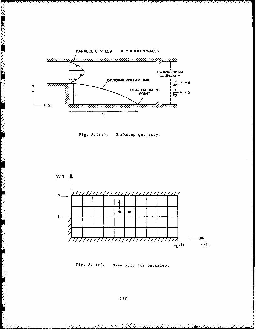
PARABOLIC IN FLOW u - 0 ON WALLS
* DOWNSTREAMBOUNDARY
xrx
y/
77/7x7~7~7~7: 7777777777
Fig. 8.1(). Begi fobackstep oer .
y150
.......................................
..............................................................

Fig. 8.2. u(x~v) for Re -100.
151

Fig. 8.3. v(x,v) for Re -100.
152
-. 7
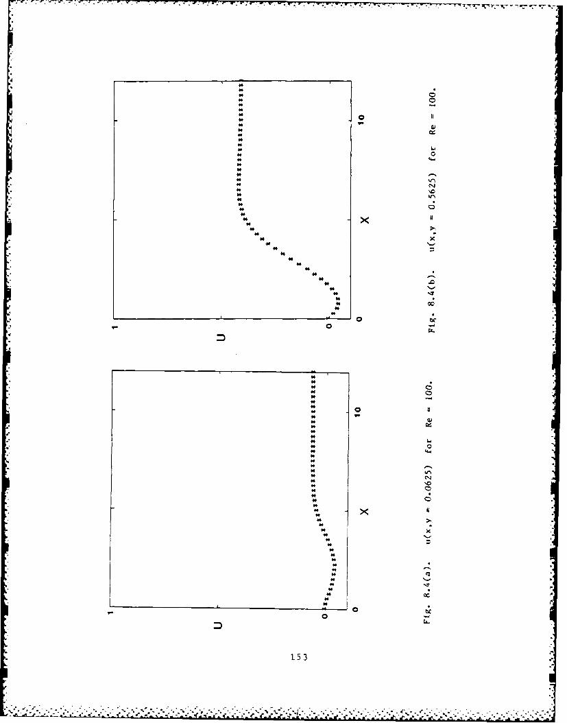
4*4*4* 04* 04*4*4*4* 04* 1~4*4*4*4*4*4* 04*4*4*4*4* L1~
4* c-.J4*4*4*4* 04*4*
4*4*
4*4*
4*44
4*.4
4*4*
4*4*
4* -'4*
4*4* '.7
4*4*4*
4*'~ 00 '-4
4*4*4* 04* 04* -4*4*4* 04*4*4*4*4*4*4* 04*4*4*4*4* Lr%4*4*4* '04* 04*4* 04*
4*4*4*
4* x4*
4*4*4*4*4*4*4* -~4*4*
4* -.7 p
4*
4*
4* 00
153
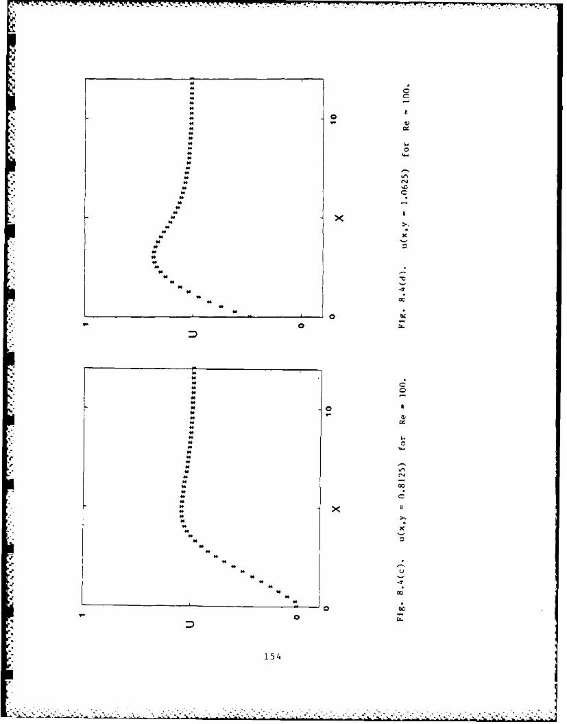
0.000.4
00
4
4
.4n406
.4
4
4
.44
.4C
. 0
.- 4
.15

4w
44
444
644
0004*
4444
444444 1
44
444404
40 44
06 44
40 40
155C


0 01CLI
C C
4-i
6
ov 00 , 40
Mo 0 0
.44
0 40
o 40
0 0
owo
157~
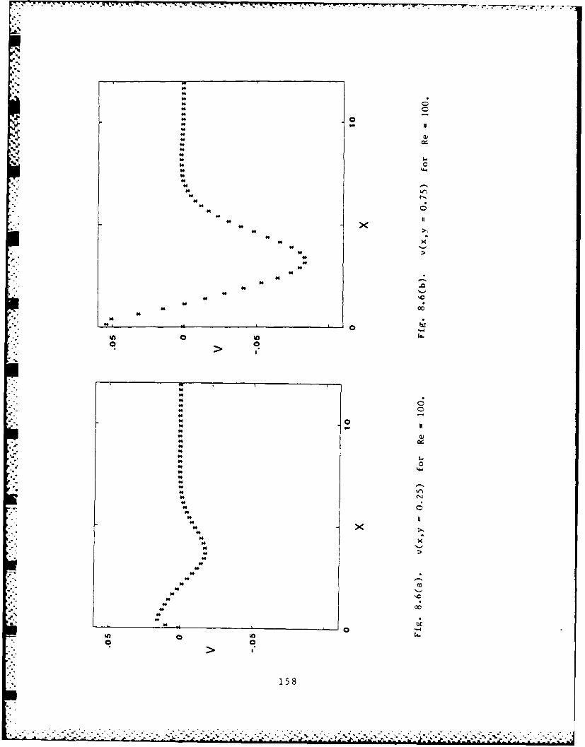
4.40
4
to
40
** 6^
40.
to
ft
4.
4
4.
.P 4.
04 4.4
158

.~~~.-'v'~~ -.'' ~ -~ V T-w- - .Fur Yw~ . -. - -x -PW - U P
4
.4n
.4 0
.40
.04
.P6
.4
.4-
co440
.40
.15

-J ,
p.J
w0
I0
4.
0
._ 160

,ira
tmC
NC
4* *
.4
.4
.4m
.4 .4
Nc
.4 4 -
.4 II
. 4•
[ . . . .. +:. -. - . .- -: -.- , . .. + . :_+- + . , . 4 . : . + ., +. : .. . + - . 4 I.a,- - -- X+ - -: , - . . . ; : + . . +2 . . .. .. : . +
€ 161

0
C
II
II
IC xo
IC
o,0
162
, - .. - . .. - .. . . . . . • . , " , ' . • . . . • . •
-'. ..'- -.. -' -" '... .-." - -. ' . , -'. , -' - " " " ' . " '- . .°' -' .' . " . " . .' ' ' ' ' - .' .' ' ' L ' + " " ' "- -'-

V-o
x -S4N v co M
cm 0 0 x
x 0 0x *o
x N
o .4
C44 co t
slaml
44
x .4HN
163
70
o U
Co]

C4.v
0c~100 .4
I.x 0
N
N .0
N
PbV
00
.16

-70
CA
a x
o 6
*c
0 0
*x
IC
-,
0CL)
00
n ul JIJ3 S0
I-6

.. . . . . .
yI
0
x
2166
............................. ..................
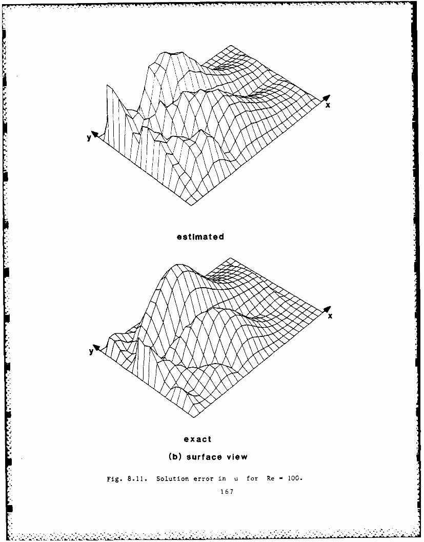
.V1
estimated
exact
(b) surface view
Fig. 8.11. Solution error in u for Re 100.
167

no
y.
exact
estimantorve
Fi.81. Slto rrri o e 10
y __ __ __ __ __ __ __ __ __ __ __ __ __168_ __

/yJx
estimated
exact
(b) surface view
Fig. 8.12. Solution error in v for Re -100.169

y
xestimated
LL
204
x
exact
(a) contour view
Fig. 8.13. Truncation error in u for Re 100.
170

estimated
exact
(b) surface view
Fig. 8.13. Truncationi error in u for Re -100.
171
. ~ ~ ~ - L. .- , - -

y _ _ _ _ _ _ _ _ _ _
L-2I
estimated
y .. __. _ _._. __._.__._._.__._.__ ._I__ I_ I__ I_ I
IN
exact
(a) contour view
Fig. 8.14. Truncation error in v for Re -100.
172
IL

estimated
Soex act
(b) surface view
Fig. 8. 14. Truncation error in v for Re =100.
173

(a)
Fig. 8.15. Rotated refined rectangles for backstep.
XL2 XL1 XL =XL
Fig. 8.16. Notation for refined grids.
174

0 u
10-E
0 48
Iteration No., mn
Fig. 8.17. Convergence of active method on two-level grid system.
175

8 08x8088%
Um 0
o0
-J
0 C0
ox u
0 0
Oox 0
~1 ox o
po 0Uo mt
00
0 x a a
S176

140
12
10
6
4
0 data from Armaly2 - computation of Kim &Momn
8s Present results
0 200 400 600Re
Fig. 8.19. Reattachment length vs. Reynolds iumber.
17 7

R D-Al69 471 ADPTIVE GRID TECHNIQUES FOR ELLIPTIC FLUID-FLOWi 3a'
ft PROBLENS(U) STANFORD UNIV CA CENTER FOR LARGE SCALEI SCIENTIFIC COMPUTATION S C CARUSO ET AL. DEC 65
UNCLASSIFIED CLRSSIC-05-19 NOSSS4-92-K-015 F/O 20/4 UL

-~4 11 2.8 2.5- . - 2
4
- a3.6.
AI
MICROCOPY RESOLUTION TEST CHART
NATIONAL BQRE AU 01 bTANDA DS- 1963-
Np.
% %
: :::N:
i c : i __
- 3 °2 .
": (9 v'

r~ousPA l
Chapter 9 s
CONCLUSIONS AND RECOMMENDATIONS
In this research, we have developed adaptive grid techniques for
flows governed by the incompressible Navier-Stokes equations. The local
refinement method of Berger, developed for hyperbolic equations, was
extended to elliptic equations. Specifically, we implemented two fea-
tures of Berger's method: overlaid, locally uniform grid refinement
consisting of rotated rectangles, and refinement regions defined by
Richardson error estimates.
Local refinement offers the following important advantages over
global refinement methods:
* lower computational overhead,
* no instability or skewness problems associated with grid-point distribution,
* truncation error used for refinement criterion,
* less reliance on heuristic criteria and problem-dependeitparameters,
* solution accuracy explicitly addressed.
Two classes of elliptic flows were identified; they are character-
ized as having strong or weak viscous-inviscid interactions. Adaptive
solution methods, active and passive, respectively, were developed for
each class.
Application of the passive method to linear, two-point boundary-
value problems demonstrated the feasibility of the solution technique.
The method is efficient compared to using a uniform fine grid.
The passive method was also applied to a 2-D, linear convection-
diffusion problem, in which the flow is oblique to the grid lines. The
refined grids automatically aligned with the flow, thereby minimizing
numerical diffusion. For fixed accuracy, the adaptive method is signif-icantly more efficient than using a uniform grid.
The SIMPLER method was used to solve the steady, laminar, incom-
pressible Navier-Stokes equations. Central differencing of the con-
vective terms was implemented with the defect-correction method to
179
,L L A

stabilize the solution method for all cell Reynolds numbers. Smooth
solutions were calculated for cell Reynolds numbers as high as 150,
indicating that the commonly used restriction, ReAx < 2, is too
severe.
Uniform grid calculations were performed for the laminar backstep
flow. Patankar's power-law scheme was shown to be less acccurate than
central differencing, and only first-order accurate.
The Richardson-estimated solution and truncation errors were also
compared to accurate estimates of the same quantities for the backstep
flow. The solution error is predicted well. The truncation-error
estimates are less accurate, but they reliably indicate where grid
refinement is required.
Active-adaptive calculations of the backstep were made, using
boundary-aligned refinement. At Re - 100, the adaptive calculation
has comparable accuracy but is six times faster than a uniform-grid
calculation. Adaptive calculations were also made at higher Reynolds
numbers. The calculations agree well with the experimental data and
other calculations.
Recommendations
Several aspects of our adaptive technique should be further studied
and improved. First, the method has been developed for rectangular
problem domains; extension to complex geometries will increase the
method's usefulness as an engineering tool.
Interpolation methods for rotated grids need to be developed. The
issue of conservation and how it is maintained using local grid refine-
ment needs to be better understood. Also, to increase the adaptive
efficiency, higher-order interpolation methods, preferably cubic inter-
polation, for fine-grid boundary conditions are recommended.
The convergence rate of the active solution method is probably not
optimum. It should he determined what is the best iteration strategy--
to iterate for a fixed number of times (and how many) or to iterate to a
partial convergence on each grid before switching. The choice probably
depends on the problem and also the Reynolds number.18
", 180

Since the active method is similar to multigrid methods (which are
very efficient), the techniques used to improve multigrid convergence
rates may be applicable to the active method; this should be further
evaluated. For example, different sweep patterns may prove more effi-
cient; e.g., "W" sweeps, the so-called Full Multigrid (FMG) cycle, etc.
Also, when switching from a coarse to a fine grid in a multigrid method,
the fine grid solution is corrected at all internal fine grid points.
Recall that, in the active method, only the fine grid boundary condi-
tions are interpolated from the coarse grid. Addition of such a correc-
tion may improve the overall convergence rate.
Finally, the method should be extended to the Reynolds-averaged
equations and also to three dimensions. Stch flows pose some of the
most challenging engineering problems.
-. . .

- . - . - -. . - - - L b .. - . S Sb
A,
4
A..
A'
A..
"A.
A-
.d.-A
A.
4
182

REFERENCES
Allen, D. N. de G., and R. V. Southwell (1955), "Relaxation MethodsApplied to Determine the Motion, in Two Dimensions, of a ViscousFluid Past a Fixed Cylinder," Q. J. Mech. Appl. Math., Vol. 8, p.129.
Anderson, D. A. (1983). "Adaptive Grid Methods for Partial DifferentialEquations," in Advances in Grid Generation, ASME Fluids Engrg. Con-ference, Houston.
Anderson, D. A., and M. M. Rai (1982), "The Use of Solution AdaptiveGrids in Solving Partial Differential Equations," in Numerical GridGeneration (J. F. Thompson, ed.), North-Holland, New York.
Armaly, B. F., F. Durst, J. C. F. Pereira and B. Schonung (1983), "Ex-perimental and Theoretical Investigation of Backward-Facing StepFlow," Jnl. Fluid Mech., Vol. 127, pp. 4 73-4 96 .
Atta, E. H., and J. Vadyak (1983), "A Grid Overlapping Scheme for F'ow-field Computations about Multicomponent Configurations," AIAA Jnl.,Vol. 21, No.1, pp. 12 7 1-12 77 .
Auzinger, W., and H. J. Stetter (1982), "Defect Corrections andMultigrid Iterations," in Lecture Notes in Mathematics, #960:Multigrid Methods, Springer-Verlag.
Babuska, I., J. Chandra and J. E. Flaherty (1983), Adaptive Computa-tional Methods for Partial Differential Equations, SIAM, Philadel-phia.
Bai, D. (1984), "Local Mesh Refinement Multilevel Techniques," Ph.D.Thesis, Dept. of Applied Mathematics, Weizmann Institute, Israel.
Bender, C. M. and S. A. Orszag (1978), Advanced Mathematical Methods forScientists and Engineers, McGraw-Hill, New York.
Berger, M. J. (1982), "Adaptive Mesh Refinement for Hyperbolic PartialDifferential Equations," Ph.D. Thesis, Dept. of Computer Science,Stanford University, Calif.
Berger, M. J. (1983), "Data Structures for Adaptive Mesh Refinement," inAdaptive Computational Methods for Partial Differential Equations(I. Babuska, J. Chandra and J. E. Flaherty, eds.), SIAM,Philadelphia.
Berger, M. J. (1984a), personal communication.
Berger, M. J. (1984b), "On Conservation at Grid Interfaces," ICASE Rept.No. 84-83, NASA Langely Res. Ctr.
Berger, M. J. and J. Oliger (1984), "Adaptive Mesh Refinement for Hvper-bolic Partial Differential Equations," Jnl. Comp. Phy., Vol. 53,pp. 48 4-512.
183
* *: "."

Berger, M. J. and A. Jameson (1985), "Automatic Adaptive Grid Refinementfor the Euler Equations," AIAA Jnl., Vol. 23, No.4, pp. 561-568.
Bolstad, J. H. (1982), "An Adaptive Finite Difference Method for Hyper-bolic Systems in One Space Dimension," Ph.D. Thesis, Dept. ofComputer Science, Stanford University, Calif.
Brackbill, J. U. (1982), "Coordinate System Control: Adaptive Meshes,"in Numerical Grid Generation (J. F. Thompson, ed.), North-Holland,New York.
Brandt, A. (1977), "Multi-Level Adaptive Solutions to Boundary ValueProblems," Math. Comp., Vol. 31, No. 138, pp. 333-390.
Brandt, A. (1982), "Guide to Multigrid Development," in Lecture Notes inMathematics, #960: Multigrid Methods, Springer-Verlag.
Brown, D. L. (1982), "Solution Adaptive Mesh Procedures for the Numeri-
cal Solution of Singular Perturbation Problems," Ph.D. Thesis,Dept. of Applied Mathematics, California Institute of Technology,Calif.
Chorin, A. J. (1968), "Numerical Solution of the Navier-Stokes Equa-tions," Math. Comp., Vol. 22, pp. 745-762.
Dihn, Q. V., R. Glowinski, and J. Periaux (1984), "Solving Elliptic
Problems by Domain Decomposition Methods with Applications," inElliptic Problem Solvers II (Birkhoff and A. Schoenstadt, eds.),Academic Press, Orlando, Fla.
Dorr, F. W. (1970), "The Numerical Solution of Singular Perturbations of
Boundary Value Problems," SIAM Jnl. Numer. Anal., Vol.7 , No.2,June.
Durst, F. and J.C.F. Pereira (1983), "Calculation of Laminar Backward-Facing Step Flow with Four Discretization Schemes for the Convec-tion Terms," GAMM Workshop, Bievres, France.
Dwyer, H. A. (1984), "Grid Adaption for Problems in Fluid Dynamics,"AIAA Jnl., Vol. 22, No. 12, pp. 1705-1712.
Dwyer, H. A., R. J. Kee, and B. R. Sanders (1980), "Adaptive GridMethods for Problems in Fluid Mechanics and Heat Transfer," AIAAJnl., Vol. 18, No. 10, pp. 1205-1212.
Dwyer, H. A., M. D. Smooke, and R. J. Kee (1982), "Adaptive Gridding forFinite Difference Solutions to Heat and Mass Transfer Problems," inNumerical Grid Generation (J.F. Thompson, ed.), North-Holland, New
York.
Ferziger, J. H. (1983), "Higher Level Simulations of Turbulent Flow," in
Computational Methods for Turbulent, Transonic and Viscous Flows,(J.-A. Eessers, ed.), Hemisphere PublishinR Corp, New York.
.
184J" "" -, - , t -, t .1 . .. .. . .' " :" - ' ' ' ' , ' ' ' ' ' ' " .
'

-. I. . ...- ,_1 .y --
Ferziger, J. H. (1986), "Simulation of Incompressible Turbulent Flows,'paper submitted to Jnl. Comp. Phy.
Fuchs, L. (1985), "Multi-Grid Solutions on Grids with Non-Aligning Coor-dinates," paper presented at Second Copper Mountain Conference on
Multigrid Methods, April 1-3, Copper Mountain, Colorado.
, Gladwell, I., and R. Wait (1979), A Survey of Numerical Methods for
Partial Differential Equations, Clarendon Press, Oxford.
Gnoffo, P. A. (1982), "A Vectorized, Finite Volume, Adaptive-Grid Algo-
rithm for Navier-Stokes Calculations," in Numerical Grid Genera-tion, (J. F. Thomoson, ed.) North-Holland, New York.
Gnoffo, P. A. (1983), "A Finite Volume, Adaptive Grid Algorithm Appliedto Planetary Entry Flowfields," AIAA Jnl., Vol. 21, No. 9, pp.1249-1254.
Greenburg, J. B. (1985), "A New Self-Adaptive Grid Method," AIAA Jnl.,Vol. 23, No. 2, pp. 317-320.
Gropp, W. D. (1980), "'A Test of Moving Mesh Refinement for 2-D ScalarHyperbolic Problems," SIAM Jnl. Sci. Stat., Vol. 1, No. 2, pp. 191-197.
Hageman, L. A., and D. M. Young (1981), Applied Iterative Analysis,Academic Press, New York.
Han, T., J.A.C. Humphrey, and B. E. Launder (1981), "A Comparison ofHybrid and Quadratic-Upstream Differencing in High Revnolds NumberElliptic Flows," Comp. Meth. Appl. Mech. and Eng., Vol. 29, pp. 81-
Harlow, F. T., and J. E. Welch, "Numerical Calculations of Time-
Dependent Viscous Incompressible Flow of Fluid with Free Surface,"Phy. Fluids, Vol. 8, No. 12, pp. 2182-2189.
Hedstrom, G. W., and G. H. Rodrigue (1982), "Adaptive Methods for Time-Dependent Partial Differential Equations," in Lecture Notes inMathematics #960: Multigrid Methods, Springer-Verlae.
Hemker, P. W. (1981), "An Accurate Method Without Directional 9ias for
the Numerical Solution of a 2-D Elliptic Singular PerturbationProblem," Rept. NW 117/81, Dent. of Numerical Mathematics, Center
of Mathematics, Amsterdam.
Hessenius, K. A., and M. M. Rai (1984), "Applications of a Conservative
Zonal Scheme to Transient and Geometricallv Complex Problems," AIAAPaper No. 84-1532.
l'in, A. M. (1969), "Differencing Scheme for a Differential Equationwith a Snall Parameter Affectins the Highest Derivative," Math.
Notes, Vol. 6, pp. 596-602.
185
€-'- "-"-...........................'. .... -. -... .... ... "." .."" .."." .

-. ,. ..- .... ° o
Jameson, A., "Iterative Solution of Transonic Flows over Airfoils andWings, Including Flows at Mach I," Comm. Pure Appl. Math., Vol.
XXVII, pp. 283-309.
Kang, L. S., Y. P. Chen, L. L. Sun, and H. Y. Quan (1985), "A Class ofNew Asynchronous Parallel Algorithms for Solving Partial Differen-tial Equations," Mathematical Research Report No. 19, WuhanUniversity, Wuhan, China, (in English).
Kellog, R. B., and A. Tsan (1978), "Analysis of Some Difference
Approximations for a Singular Perturbation Problem Without TurningPoints," Math. Comp., Vol. 32, No. 144, pp. 1025-1039.
Kim, J., and P. Moin (1985), "Application of a Fractional-Step Method toIncompressible Navier-Stokes Equations," Jnl. Comp. Phys., Vol. 59,pp. 308-323.
Kline, S. J., B. J. Cantwell, and G. M. Lilley (1982), The 1980-81AFOSR-HTTM- Stanford Conference on Complex Turbulent Flows,Mechanical Engrg. Dept., Stanford University, Stanford, CA.
Kreiss, B., and H. 0. Kreiss (1981), "Numerical Methods for SingularPerturbation Problems," SIAM Jnl. Numer. Anal., Vol. 18, No.2, pp.262-276.
Leonard, B. P. (1979a), "A Stable and Accurate Convective ModellingProcedure Based on Quadratic Upstream Interpolation," Comp. Meth.Appl. Mech. and Eng., Vol. 19, pp. 59-98.
Leonard, B. P. (1979b), "A Survey of Finite Differences of 0pinion onNumerical Muddling of the Incomprehensible Defective ConfusionEquation," in Finite Element Methods in Convection Dominated Flows,(T. Hughes, ed.), ASME WAM, New York.
Leschziner, M. A. (1980), "Practical Evaluation of Three Finite Differ-ence Schemes for the Computation of Steady-state RecirculatingFlows," Comp. Meth. Appl. Mech. and Eng., Vol. 23, pp. 293-312.
Leschziner, M. A., and W. Rodi (1981), "Calculation of Annular and TwinParallel Jets Using Various Discretization Schemes and Turbulence-!odel Variations," Jnl. Fluids Eng. Vol. 103, pp. 352-360.
Mastin, C. W. (1982), "Error Induced by Coordinate Systems," in Numer-ical Grid Generation (J.F. Thompson, ed.), North-Holland, New York.
Mehta, U. B. (1984), "Physical Aspects of Computing the Flow of a Vis-cous Fluid," NASA TM 85893, Ames Res. Ctr.
Miller, K. (1965), "Numerical Analogs to the Schwarz Alternating Proce-
dure," Numer. Math., Vol. 7, pp. 91-103.
Murman, E. M., and J. R. Baron (1983), "Computational Methods for Com-plex Flowfields," 1983 Annual Report, AFOSR-TR-83-0841
186

Nakahashi, K. and G. S. Diewert (1984), "A Practical Adaptive-GridMethod fur Complex Fluid-Flow Problems," NASA TM-85989, Ames Res.Ctr.
Nakahashi, K., and G. S. Diewert (1985), "A Three-Dimensional AdaptiveGrid Method," AIAA Paper No. 85-0486.
Oliger, J. (1984), "Adaptive Grid Methods for Hyperbolic Partial Differ-ential Enuations," in Inverse Problems of Acoustic and ElasticWaves (F. Santosa, Y.-H. Pao, W. W. Symes and C. Holland, eds.),SIAM, Philadelphia.
Patankar, S. V. (1980), Numerical Heat Transfer and Fluid Flow, Hemi-sphere Publishing Corn., New York.
Patankar, S. V. (1981), "A Calculation Procedure for Two-DimensionalElliptic Situations," Numerical Heat Transfer, Vol. 4, pp. 40 9 -4 2 5 .
Pearson, C. E. (1968), "On a Differential Equation of Boundary LayerType," Jnl. Math. and Phys., Vol. 47, pp. 134-154.
Pearson, C. E. (1981), "Use of Streamline Coordinates in the NumericalSolution of Compressible Flow Problems," Jnl. Comn. Phvs., Vol. 42,pp. 257-265.
Peyret, R., and T. D. Taylor (1983), Computational Methods for FluidFlow, Springer-Verlag, New York.
Pierson, B. L., and P. Kutler (1980), "Optimal Nodal Point Distributionfor Improved Accuracy in Computational Fluid Dynamics," AIAA Jnl.,Vol 18, No. 1, pp. 49-54.
Rai, M. M (1985), "An Implicit, Conservative, Zonal-Boundary Scheme forEuler Equation Calculations," AIAA Paper No. 85-0488.
Rai, M. M., and D. A. Anderson (1981a), "Grid Evolution in Time Asymp-totic Problems," Jnl. Comp. Phys., Vol. 43, pp. 327-344.
Rai, M. M., and D. A. Anderson (1981b), "The Use of Adaptive Grids inConjunction with Shock Capturing Methods," AIAA Computational FluiiDynamics Conference, Palo Alto, CA.
Raithby, G. D. (1976), "Skew-upstream Differencing Schemes for ProblemsInvolving Fluid Flow," Comp. Meth. Appl. Mech. Eng., Vol. 9,pp. 151-162.
Reynolds, W. C. (1976), "Phenomenological Turbulence Modeling," in Ann.Revs. Fluid Mech., Vol. 8, p. 183.
Roache, P. J. (1982), Computational Fluid Dynamics, Hermosa Publishers,Albuquerzue, N.M.
Rodi, W. (1980), Turbulence Models and Their Applications in Hydraulics,Intl. Assn. for Hydraulics Research, Delft.
187

Rodrigue, G., and J. Simon (1983), "A Generalization of the NumericalSchwarz Algorithm," Lawrence Livermore Laboratory Report ikUCRL-90030.
Saltzman, J., and J. Brackbill (1982), "Applications and Generalizationsof Variational Methods for Generating Adaptive feshes," in Numeri-cal Grid Generation (J.F. Thompson, ed.), North-Holland, New York.
Shyy, W. (1985), "A Study of Finite Difference Approximations to Steady-State, Convection-Dominated Flow Problems," Jnl. Comp. Phy., Vol.57, pp. 415-438.
Smith, G. D. (1978), Numerical Solution of Partial Differential Equa-tions: Finite Difference Methods (second ed.), Oxford UniversityPress, London.
Spalding, D. B. (1972), "A Novel Finite-Difference Formulation forDifferential Expressions Involving Both First and Second Deriva-tives," Int. J. Num. Methods Eng., Vol. 4, p. 551.
Starius, G. (1977), "Composite Mesh Difference Methods for EllipticBoundary Value Problems," Numer. Math., Vol. 28, pp. 243-258.
Stetter, H. J. (1978), "The Defect Correction Principle and Discre-tization Methods," Numer. Math., Vol. 29, pp. 425-443.
Stoutemyer, D. R. (1972), "Numerical Implementation of the SchwarzAlternating Procedure," Ph.D. Thesis, Dept. of Computer Science,Stanford University, Calif.
Tang, W. P., W. Skamarock, and J. Oliger (1985). To appear.
Thompson, J. F. (1984), "Grid Generation Techniques in Computational
Fluid Dynamics," AIAA Jnl., Vol. 22, No. 11, pp. 1505-1523.
Thompson, J. F. (1983), "Dynamically-Adaptive Grids in the NumericalSolution of Partial Differential Equations," IFIP Conference on PDE
Software, Soderkoping, Sweden.
Van Leer, B. (1979), "Towards the Ultimate Conservative Difference
Scheme. V. A Second-Order Sequel to Codunov's Method," Jnl. Comp.Phys., Vol. 32, pp. 101-136.
Zabusky, N. J., and G. S. Deem (1971), "Dynamical Evolution of Two-dimensional Unstable Shear Flows," Jnl. Fluid Mech., Vol. 47, Pt.2, pp. 353-379.
Zebib, A., and G. M. Homsy (1984), "Laminar Flow Over a Backward-FacingStep," Manuscript #84-07, Center for Large Scale Scientific Compu-tation, Stanford University, Stanford, CA.
Zehib, A. (1984), personal communication.
!185

Appendix A
QUANTIFICATInN OP THE STRENGTH OF THE VISCOUS-INVISCID INTERACTION
In this appendix, we show how the strength of the viscous-inviscid
interaction can be auantified for the flow in the inlet region of a
plane channel. The same methodology can be applied to other flows. It
is required only that the boundary-layer displacement thickness can be
related to velocity in the inviscld, outer region.
The displacement thickness 6 for a constant-density fluid is
defined as:
6
6 = j (Vo-v) dy (A.1)
0
where 6 is the boundary-layer thickness, V the velocity outside,0
and v the velocity inside the boundary laver (see Fig. 3.1). 6 is a
measure of the boundary-layer thickness. For the flow over a flat
plate, 6* 6/3.
The displacement thickness has the following significance. The
uniform, inviscid flow at velocity V0 through a channel, whoge
height L has been reduced (displaced) by an amount equal to 6* on
each end, will have the same volumetric flow as the viscous flow through
a channel of height L. The inviscid flow is coupled to the viscous
flow in the boundary layer through this displacement effect.
The displacement thickness is related to V by:0
V = Q (A.2)
L - 26
where n, the volumetric flow through the cThannel, is:
0 - L (A.3)
and V is the average velocity in the channel. q'ibstititiqg (k.3) into
(A.2) gives:
1 10 1 25
189
I-. ...

whe re
V *
v1 -, ; S . - (A.5)
V
If the displacement thickness is increased by an amount A6*, the outer
velocity becomes:
0(6 A6 (A.6)
I - 2(6 + A6 )
where we have dropped the ' ". Subtracting (A.4) from (A.6) and
dividing the result by (A.4) gives the following relationship for the
relative change in V:
+) - 2 6 (A.7)o *=*- - 1 (A.7)
Vo Vo(6*) 1 - 2(6* + A6*)
Let the change in 6 be:
A6 = (K-I) 6 (A.8)
where K is a sensitivity parameter. Substituting (A.8) into (A.7)
gives the desired result:
AVo 2(K-I) 6 (A.9)V *o 1 - 2K6
Equation (A.9) quantifies the strength of the coupling between the
boundary layer and the outer, inviscid flow.
AV /V is plotted in Fig. 3.2, for K = 2,10. On a coarse grid,
the boundary layer may be smeared to twice its actual size, K = 2. The
relative change in Vo should be no greater than the maximum allowable
error. For K 2 2 and maximum allowed error, 0.1%, the coupling is
weak for 6*/L < 10- 3 , and strong at larger 6* /L.
190
........................................ . . . . . . . . .. . . . . . . . . .-.. .-

-~. ...-- -p -- ~ - v;. - - -- -. - -
4
44
.4
- t
d
4
.4
4
p-- #- .- .- -p -- -I ~ -. *p *~ ~-* ... ... .*...--*.(*-.* -... *- . -. *p*~*~* .. . . - .j.
. . .. . V..