technique for predicting the radio frequency field ... · technique for predicting the radio...
TRANSCRIPT

NASA Technical Memorandum 104646
/H-_3
,/
Technique for Predicting the Radio
Frequency Field Strength Inside anEnclosure
Michael P. Hallett and Jerry P. Reddell
May 1997
https://ntrs.nasa.gov/search.jsp?R=19970018387 2018-05-28T16:28:34+00:00Z


NASA Technical Memorandum 104646
Technique for Predicting the Radio
Frequency Field Strength Inside anEnclosure
Michael P. Hallett
Goddard Space Flight Center
Greenbelt, Maryland
Jerry P. Reddell
McDonnell Douglas
Seabrook, Maryland
National Aeronautics and
Space Administration
Goddard Space Flight CenterGreenbelt, Maryland
1997

This publication is available from the NASA Center for AeroSpace Information,
800 Elkridge Landing Road, Linthicum Heights, MD 21090-2934, (301) 621-0390.

Abstract
This Memorandum presents a simple analytical technique for predicting the RF electric field strength
inside an enclosed volume in which radio frequency radiation occurs. The technique was developed to
predict the radio frequency (RF) field strength within a launch vehicle's fairing from payloads launched
with their telemetry transmitters radiating and to the impact of the radiation on the vehicle and payload.
The RF field strength is shown to be a function of the surface materials and surface areas. The method
accounts for RF energy losses within exposed surfaces, through RF windows, and within multiple layers of
dielectric materials which may cover the surfaces. This Memorandum includes the rigorous derivation of
all equations and presents examples and data to support the validity of the technique.
°°.111


Table of Contents
Section Page Number
1.0 Introduction ....................................................................................................................................... 1
2.0 Analytical Concept ............................................................................................................................ 1
3.0 Analytical Steps ................................................................................................................................. 2
4.0 Summary of Background and Efforts ................................................................................................ 2
5.0 Validation of the Analytical Model .................................................................................................... 3
5.1 Acoustic Blanket Modeling ...................................................................................................... 3
5.1.1 Classical Theory ........................................................................................................... 4
5.1.1.1 Half Wavelength Characteristics ..................................................................... 4
5.1.1.2 Quarter Wavelength Characteristics .............. .................................................. 5
5.1.1.3 Shorted and Opened Transmission Line ......................................................... 8
5.1.1.4 Classical Theory Conclusions on Equation ..................................................... 9
5.1.2 Cover Sheet Model Validation ...................................................................................... 9
5.1.3 Blanket on RF Window Model Validation ................................................................. 10
5.1.4 Conclusion on Acoustic Blanket Modeling ................................................................ 10
5.2 Validation of the Basic Technique .......................................................................................... 105.2.1 Bare Aluminum Walls ................................................................................................. 10
5.2.2 Small Area of Blanket-Covered Wall ......................................................................... 11
5.2.3 Large Area of Blanket-Covered Walls ........................................................................ 11
5.2.4 Aluminum Room Model Conclusions ........................................................................ 12
5.3 Vehicle Validation ................................................................................................................... 14
5.3.1 KoreaSat RF Measurements ....................................................................................... 14
5.3.2 XTE Mission RF Levels ............................................................................................. 14
5.3.3 Composite Fairing Testing .......................................................................................... 15
5.3.3.1 Bare Composite Fairing Test ......................................................................... 15
5.3.3.2 Composite Fairing with Acoustic Blanket Test ............................................. 15
5.3.4 Vehicle Validation Conclusions .................................................................................. 15
6.0 Recommendation for composite Fairing ......................................................................................... 15
6.1 Replace Aluminized Kapton ................................................................................................... 15
6.2 Stabilize the Thickness of the Blanket ................................................................................... 16
6.3 Select Proper Combination of Blanket Thickness .................................................................. 16
6.4 Make the Melamine Foam Conductive .................................................................................. 16
7.0 Conclusions ..................................................................................................................................... 17
Appendix A. A Method for the Estimation of the Field strength of Electromagnetic Waves Inside a
Volume Bounded by a Conductive Surface .................................................................... A-1
Appendix B Derivation of Equation for Electric Field Inside an Enclosure ...................................... B-1
B.1 Introduction ................................................................................................................................... B-2
B.2 Equations for the Boundary of Two Media ................................................................................... B-2
B.2.1 Boundary Conditions of Media 0 and Media 1 ................................................................. B-3

J
_. ii
B.3 Determine the Equations for the Waves in Each Media ............................. ................................... B-6
B.3.1 Derive the Equations for the Incident Wave ...................................................................... B-6
B.3.2 Reflected Wave Equations ................................................................................................. B-7
B.3.3 Determine the Equations for the Transmitted Wave .......................................................... B-9
B.4 Power for a Plate of Multiple Materials ...................................................................................... B-11
B.4.1 Power of the Incident Wave on Multiple Materials ......................................................... B-11
B.4.2 Power of the Reflected Waves from Multiple Materials ................................................. B-12
B.4.3 Power Entering the Several Materials ............................................................................. B-12
B.5 Determine the E Field in an Enclosure ........................................................................................ B-13
B.5.1 Value of the Incident Wave in the Enclosure ................................................................... B-13
B.5.2 Standing Wave in the Enclosure ...................................................................................... B-13
B.6 Conclusions ................................................................................................................................. B-14
Appendix C. Derivation of the Equations for a Media's Intrinsic Characteristics .............................. C-1
C.1 Introduction ................................................................................................................................... C-2
C.2 Wave Impedance ............................................................................................................................ C-2
C.2.2 Wave Propagation Constants ............................................................................................. C-7
C-3 Other Characteristics ................................................................................................................... C-11
C.3.1 Wave Velocity in the Media ............................................................................................. C-11
C.3.2 Wavelength in a Media .................................................................................................... C-11
C.3.3 Skin Depth ....................................................................................................................... C-11
C-4 Summary ...................................................................................................................................... C-12
Appendix D. Method for Determining the Effective Impedance of the Acoustic Blankets on a
Surface ............................................................................................................................ D- 1
D.1 Introduction ................................................................................................................................... D-2
D.2 Approach ....................................................................................................................................... D-2
D.3 Equivalent Impedance of a Material Boundary by Two Media ..................................................... D-3
D.4 Transmittance Through a Media of Thickness, T .......................................................................... D-6
D.5 Application to the Acoustic Blanket Installation ........................................................................... D-7
D.5.1 Impedance of the Fairing Wall .......................................................................................... D-7
D.5.2 Transmittance Through the Acoustic Blanket ................................................................. D-10
D.6 Conclusion ................................................................................................................................... D-12
Appendix E. Calculating RF Characteristics of the Acoustic Blanket Cover Sheets .......................... E-1
vi

List of Figures
Figure
Figure
Figure
Figure
Figure
Figure
Figure
Figure
Figure
Figure
Figure
Figure
Figure
Figure
Figure
Figure
Figure
Figure
Figure
Figure
Figure
Figure
Title
1
2
3
4.
5.
6.
7
8
9.
10
11
B-1
B-2
B-3
D-1
D-2
D-3
D-4
D-5
D-6
D-7
Page Number
Effective Impedance of Batting on Air ............................................................................... 5
Batting on Aluminum ......................................................................................................... 6
Impedance of Batting on High Impedance Plate ................................................................ 6
The Variation of Reactance Along a Lossless Short-circuited Line ................................... 7
Reactance of Batting on Aluminum .................................................................................... 7
The Variation of Eeactance Along a Lossless Open-circuited Line ................................... 8
Reactance of Batting on High Impedance .......................................................................... 8Effect of Acoustic Blanket on Maximum Fields .............................................................. 11
Effect of Blanket Thickness on Field Strength inside Enclosure ..................................... 12
Effect of Blanket Thickness on Equivalent Impedance .................................................... 13
Effect of Blanket Thickness on Reflectance ..................................................................... 13
RF Waves at the Boundary of Two Media ...................................................................... B-2
RF Power at Boundary with a Single Material ............................................................. B-10
RF Waves at the Boundary with Several Materials ...................................................... B-11
Layers of Material for Acoustic Blanket Installation on the Fairing Wall ..................... D-2
RF Waves at the Boundary of Two Media ...................................................................... D-3
RF Waves at Surface Boundary with Two Layers of Material ....................................... D-5
RF Waves at the Boundary of an Equivalent Surface Material ...................................... D-6
RF Wave at Boundary for Cover 2 and Fairing Wall ...................................................... D-8
Blanket Batting and Boundary with Equivalent Cover/Wall Material ........................... D-9
RF Waves at Boundary with Equivalent Material for Batting, Cover Sheet and Wall ... D-9
Title
Table 1
Table 2
List of Tables
Page Number
Carbon Loaded Cover Sheet, Insertion Loss ...................................................................... 9
RF Fields Measured in the Composite Fairing ................................................................. 15
?,
vii

_L_ _ i_i_ ¸ . I .i •

1.0INTRODUCTION
An analysis technique has been developed to predict the RF field strength, within the Delta fairing, arising
from radio frequency transmission inside the fairing. This analysis is required to evaluate the impact of the
radiation that could be caused by payloads launching with their telemetry transmitters radiating. This
memorandum discusses the development of the analytical technique (mathematically derived in Appendix
B) for predicting the RF electric field strength inside an enclosed volume in which radio frequency radia-
tion occurs. The basic analytical approach is presented in Appendix A and Reference (2).
The analysis provides the ability to account for losses associated with the acoustic blankets which line the
fairing wall. A method for evaluating the RF losses within the acoustic blankets is also provided and
presented in Appendix D. This memorandum provides experimental data which validates the method. The
technique is then used to estimate the RF fields inside the Delta fairing developed by the transmitters on the
KoreaSat and XTE satellites. The computations were performed using the mathmatical functions of the
Microsoft Excel spreadsheets.
The attached appendices provide rigorous derivations of all equations used in the analysis and provide
insight into the technique for acoustic blanket modeling. Thorough study of these appendices can provide
insight into the factors involved. This memorandum addresses the analytical concept, analytical steps,
summary of background and efforts, validation of the analytical model, recommendation for composite
fairing, and conclusions.
2.0 ANALYTICAL CONCEPT
The analysis is based on the technique and hypothesis presented by M. P. Hallett in Appendix A. This
concept (derived from the conservation of energy) is that the field inside the fairing will increase, due to
reflections, until all the energy being supplied by the transmitter is absorbed by the surface areas exposed
to the RF field. Due to the combined reflected and scattered waves, the magnitude of the RF field is
hypothesized to be equivalent to the magnitude of a single incident wave which would dissipate the total
transmitter RF energy in the surface areas. The approach is an application of "Poynting's theorem" which
states: The power delivered by internal sources (the payload transmitter) to a volume is accounted for by the
power dissipated in the resistance of the media (air) plus the time rate of increase in power stored in the
electric and magnetic fields in the volume plus the power leaving through the dosed surface(s).
In our problem the power dissipated in the resistance of the media (air) inside the volume is extremely
small and can be considered to be zero. Also, since the concern is for a stabilized system, the time rate of
increase of the power stored in the electric and magnetic fields in the volume has become zero. Thus the
theorem is reduced to the following: the power sUpplied by the transmitter is equal to the power leaving
through the closed surface(s).
Mathematically the concept is implemented in Appendix B, equation (B55).
2Ak_surf real -. Okk=l L('7o+ok)2

iii_<
Z
Where: P is the radiated power,
iE 0 is the absolute value of the surface incident wave,
A k-surf is the area in square meters of the surface k,
1] the complex impedance of the surface k material, and
ylk is the complex impedance of the media (air) inside the enclosure.0
This equation shows the field is dependent on the area and impedance of each surface. The impedance of
the surface areas are, in general, a function of the frequency for homogeneous materials. The acoustic
blanket covered surface area impedance is very complex being a composite function of the properties and
thickness of each material, the order of layers of material, and the impedance of the wall material.
3.0 ANALYTICAL STEPS
The analytical steps which are performed during an analysis are briefly outlined here:
a) Compute the surface area in square meters of each of the different types of materials exposed tothe RF field.
b) Compute the intrinsic RF characteristics of each material exposed to RF field. These character-
istics are usually described as complex numbers. The equations for computing the characteristics
of most materials, including air and aluminum, are provided in Appendix C.
c) Determine the effective RF impedance of the blanket covered fairing walls. The necessary math-
ematical equation derivation and the methodology used is described in Appendix D.
d) Compute the incident wave's RF electric field strength using equation (B55) of Appendix B and
the results of the three previous steps.
Appendix A and Reference (1) provide initial explanations of the method and its application to early mod-
els of the fairing. These original explanations and computations did not include, or consider, the affects ofthe acoustic blankets.
4.0 SUMMARY OF BACKGROUND AND EFFORTS
Early in the development of the Small Expendable Launch Vehicle (SELVs) service, a need arose to esti-
mate the fields created by RF radiation within the launch vehicle's fairing. At that time, no analytical tools
were readily available. Therefore, a simple test was performed using a 1-watt S-band source radiating
inside the fairing, and measuring the resulting field strength at several points inside the fairing. The results
were alarming; with measured field strengths approaching 100 v/m. Consequently, the SELVs program
does not allow RF radiation within their fairing.
During the launch processing of an Atlas-E mission, a NOAA spacecraft reported experiencing unexpected
noise and interference of instrumentation data during ground testing. The test included RF transmitter
radiation while encapsulated in the fairing. The noise and interference vanished when the transmitter was
powered off, indicating that the spacecraft was operating at the edge of its limit. The RF field levels werenot known.
Because of the SELVs data and anecdotal information from the Atlas-E program, we began to question the
validity of past decisions allowing RF radiation within the Medium Expendable Launch Vehicle (MELVs)

sevice(Delta)fairing. It appearedthatthesedecisionshadbeenbasedoneitherfreespacecalculationsofthefield strength,or similarity to anearlier(successful)mission. Neitherapproachcouldbesupportedonarigorousengineeringbasis.
We then starteddevelopmentof a methodwhich couldbe justified by soundengineeringprinciplestoestimatethefield strengthinsideafairing. Considerableeffortwasexpendedexaminingcomputationallyintensiveapproachesusingresonantcavitytheory,raytracingtheory,etc. Themathematicsinvolvedwereextensiveandtheresultsquestionable,althoughindicatingthat fields werehigh, asexpected.Theoreti-cally,a finitedifferenceprogram(suchasGEMACS)iscapableof solvingthisclassof problem.However,thephysicaldimensionsof theproblemresultedin hugematricesthatdemandedthecapabilitiesof large,fastcomputers.An additionalshortcomingwasthattheseprogramsofferedlittle visibility into thefactorsinvolved,suchasprogramimplementationlimits, or theability to varyparameterswithin themodel. Thebasictechniqueis outlinedin sections2.0 and3.0. This techniqueinvolvescomputationsthat canbeperformedwithin aspreadsheet,yieldingresultsthatarereasonablyaccurateandtendto boundtheupperlimit of the field. The reader is cautioned that this technique yields an assumed uniform field strength,not an exact solution of the field distribution.
The first attempts to model the Delta vehicle, spacecraft, and fairing resulted in very high field strengths.
Incident RF fields of about 115 volts per meter and a standing wave of about 230 volts per meter were
computed for 1 watt transmitted. Further investigation indicated that the RF window established a limiting
factor on the buildup of the internal fields. Given the typical size of the current window (approximately 0.5
m2), our model shows that the field developed by a 1 watt source would be an incident wave in the order of
30 volts per meter with a possible standing wave to 60 v/m. This is still high, and one can reasonably
question the validity of the result in light of many successful launches without indications of EMI.
A review of the various items contained within the fairing was then initiated, searching for materials that
might further reduce the fields. We concluded (and later proved by testing) that the acoustic attenuation
blankets which line the fairing are also quite effective absorbers of RF energy. This conclusion then
demanded development of a model for the acoustic blankets, thus completing our model of vehicle, space-
craft, and fairing. This blanket model and vehicle model were subsequently validated by experimental
data, as described in section 5.0 of this memorandum.
5.0 VALIDATION OF THE ANALYTICAL MODEL
The validation of the modeling is addressed in three parts. The first addresses the validation of the tech-
nique and equation for modeling the acoustic blankets; the second addresses the validity of modeling of an
enclosed aluminum room; and the third addresses validation related to the actual vehicle fairing enclosure.
5.1 ACOUSTIC BLANKET MODELING
The computations required by our model were initially frustrated by the presence of dielectric materials in
the blankets. The blankets' unknown electrical properties and the inability to accurately evaluate their
affect on the fields presented serious problems. The need for an accurate method of evaluating the acoustic
blanket's affects became the major goal in arriving at a good analytical model.

Initial evaluation of the RF losses in the acoustic blanket began as a series expansion of the reflected and
transmitted waves between the boundaries of the many layers of materials in the blanket and the fairing
wall. This initial method convinced us the blankets were a dominant factor in reducing the field strength
inside the fairing. The series expansion technique presented several difficulties which caused an increase
in efforts to define another method. A method to accurately determine the effective impedance of the area
covered by the blankets was sought. Reference (4), Section 7-08, provided the insight to allow the deriva-
tion of the Appendix D equations.
The Appendix D equation (D17) eventually proved to accurately provide the complex impedance for the
blanket covered wall area. The validity of the blanket model is confirmed by classical theory and experi-
mental testing, which demonstrates that the results are reasonably accurate.
5.1.1 Classical Theory
The RF characteristic of homogeneous materials can be computed using the known conductivity, perme-
ability and permissivity of the materials. Many texts provide simplified equations for their computation
and testify to their validity. Appendix C provides a thorough development of the generic equations, which
can be simplified, using appropriate assumptions, to the equations presented in most texts. This testifies to
their theoretical validity.
While the impedance of many materials can be easily computed, the equivalent impedance of several layers of
material is not easily computed nor is it a subject treated thoroughly or effectively in text books. The text
typically make a brief reference to transmission line corollaries, present highly simplified equations (with no
explanation of the simplifying assumptions which were used), and then launch into activities with Smith charts
etc. In contrast to this, the rigorous mathematical derivation of equation (D17) in Appendix D indicates it is
theoretically sound. This derivation makes no confusing references to transmission line theory or Smith charts.
This equation defines the complex impedance at the surface of a single layer of material (media 1) of thickness,
which covers a plate (media 2). The subscript 1, designates the single layer material and subscript 2 is the plate.
Alpha and beta are for the single layer of material (media 1). Successive application of the equation is required
to determine the impedance of several layers of materials.
_[(02 + 771) ead +(02- O,)e-ai']COS_l I + J[(T]2 + 01) ead --(02- 01)e-a'l]sin_ll_
0L(l) = "11 [[(02 "_- 771)e_'t --(02 -- 01)e-_ll]c°sfll 1+ J[(02 + 01) e_ll + (02 -- 01)e-a_l]sinfll I J
The equation matches the simplified equations (with the appropriate simplifying assumptions, (_1 = 0)
which are normally presented in text books. This correlation with the texts supports its validity. Other
evidence is also available. Since most texts use transmission line theory as a corollary for analyzing RF
transmission through media, the characteristics from transmission line theory will be used here to demon-
strate the validity of the equation application. The optics world also has corollaries to these characteristics
which will not be discussed here.
5.1.1.1 Half Wavelength Characteristics--One well known impedance characteristic of a transmission
line is that a transmission line of length equal to a multiple half wavelength behaves as if the transmission
line is not present. In other words, the load at the source is the same as the impedance terminating the line.
Equation (D17) of Appendix D was used to calculate the equivalent impedance of fiberglass batting on air
4

:
and batting on aluminum. Figures 1 and 2 show the results as a function of the batting thickness in wave-
lengths. At multiples of the half wavelength, Figure 1 shows the effective impedance to be that of air.
Figure 2 shows the effective impedance to be that of aluminum at the half wavelength points. Both ex-
amples demonstrate the effective half wavelength characteristic expected from its corollary transmission
line theory and confirm its validity.
Classical transmission line theory shows that the impedance repeats at half wave line increments. This
repeating characteristic is demonstrated in the examples shown in Figures 1, 2, 3, 5, and 7.
5.1.1.2 Quarter WaveLength Characteristics--Another characteristic suggested by the transmission
line corollary is the impedance characteristics for odd multiples of lossless quarter wavelength line which
is terminated by the characteristic impedance of the source. That is, if the line length (batting thickness) is
an odd multiple of a quarter wavelength then the equivalent impedance at the source has an imaginary part
which is zero and the real part has a minimum magnitude. Figure 1 demonstrates this low value for the
real part and a zero value for the imaginary part at the quarter wavelength intervals.
The quarter wavelength transmission line is also an impedance inverter. This characteristic says that for a
"shorted" load (a perfect conductor), on odd multiplies of quarter wavelength line, the effective impedance
is infinite. Figure 2 is for batting on aluminum and shows that the real and imaginary parts are off scale at
the odd multiple quarter wavelengths. (Actual computations were on the order of millions of ohms for
both the real and imaginary parts.) Similarly, the theory says an open circuit would be inverted to an
effective impedance of zero at the quarter wavelength distances. Figure 3 shows the computation for the
batting on an high impedance circuit and shows the expected low (zero) impedance at the quarter wave-
length.
4 381
2 379
_°_.-2 375 _.
J= _E
e-
•_-4 373 __E
-6 371
-8 369
Batting thickness in wavelengths
Figure 1, Effective impedance of batting on air.
Imag
---- Real

' /, "
u}Ei-0$ot-in
"0
Q.E
1500
1000
500
-500
-1000
-1500
I',-',,,4.0
/
/
J i Io') LO ¢0
/
/
/
I
/
Ik_t,.:.o
I
I
I
I
II
I
I
i i tL_ 03 It)
o o o ._'.,.. d co d(:3 0
|
Batting thickness in wavelengths
I
I
I I Ic_J ko T_,d "-d o
Imag
---- Real
Figure 2. Batting on aluminum,
u)
Ep.0
0C
E
1500
1000
5OO
-500
-I000
\\
\\
I I I"'_1 TM -r ,-,. i JI I I I
Imag /
.ea--/
d d de. d _ do'\ d d d dd d d d d d d o'\\ \
\ \\ \
\ \\ \
Batting thickness in wavelengths
Figure 3. Impedance of batting on high impedance plate,

.L0"I00
I
"N
e-
o
M _
_" 5""-,i
W
O <
E _3 g
e-3
0 00 0
I I 1
0.9
_ 0.8
0.75
0.7
0.65
0.6
0.55
0.5
0.4
0.35
0.25
0.2
0.15
0.1
0.05
0
Reactance in Ohms
O O Q O
I I I-t
R<mm.
O
O
o
o
O
m
O
O
__.oc-
O.
3
m,
O
,.,IP
J
f
Reactanceii ii
Do
o

d.,9
I
I
I
I
I
I
!
I
I
I ......
I
I I
I
I
I
!
I
I1)
XL=Zo
o (a)Reactance
X c = Z o
Figure 6. The variation of reactance along a Iossless open-circuited transmission line.
Et.-0t-
,m
o
0=
m
1500
1000
500
-500
-1000
-1500
-2000
Zload = 1000 +jlO00
I I I I I'.1 I I I I
Batting thickness in wavelengths
Figure. 7 Reactance of batting on high impedance.
Io
5.1.1.3 Shorted and Opened Transmission Line--The computed impedance terms also follow the clas-
sical shapes for the shorted transmission line of varying length. Figure 4 is a typical figure given in
textbooks showing the reactance for a transmission line terminated in a short circuit as a function of trans-
mission line length. Figure 5 shows the computed reactance for the batting on aluminum which matches
the Figure 4 form. Figure 6 (typically in textbooks) shows the reactance for a transmission line with an
open circuit load. Figure 7 shows the computed reactance for the batting on a plate with a relatively high
impedance, which matches the Figure 6 characteristics.

5.1.1.4 Classical Theory Conclusions on Equation--Each of these computations show that the Appen-
dix D equation (D17) agrees with the corollaries to transmission line classical theory. The equation
demonstrates the expected quarter wave inverting characteristic, the expected half wave transparency,
repeating impedance for each half wavelength, and provides the expected capacitive and inductive nature
of the impedance with length (thickness). This correlation indicates the mathematical model (equation
(D 17) of Appendix D) is valid for the application to the acoustic blanket installation in the fairing.
A significant point of this discussion is that for any given frequency, one may expect the RF impedance of
the acoustic blanket to vary as a function of the batting thickness. In fact, it will vary between a rather high
loss level (medium impedance, low reflection) defined by the cover sheet material and a rather low loss
level (small impedance or highly reflective) defined by the wall behind the blanket. This leads us to still
another observation. At S-band frequencies, it is theoretically possible for the blankets to become "trans-
parent" due to compression and billowing, leaving the RF window the dominant factor in establishing the
upper boundary of the RF field. This will be discussed in greater detail in sections 4.5 and 4.6.
5.1.2 Cover Sheet Model Validation
Determination of the characteristics of the blanket's cover sheets is difficult because it is not a homoge-
neous material. It is made of several layers of different material. Fortunately the composite properties can
be determined experimentally by insertion loss measurements. The measurements provide the complex
dielectric constant and loss tangent at various frequencies. Test data on the carbon loaded cover sheets of
the acoustic blankets was provided by McDonnell Douglas Aerospace (MDA). This data defined the
sheet's thickness, dielectric constant, loss tangent, insertion loss, phase angle, and conductivity. Appendix
E provides the equations for computing the resistance, impedance, attenuation, and phase shift constants
for the sheet using the complex dielectric constant and the loss tangent. The Appendix E equations com-
puted comparable results to the test data. These cover sheet computations results were used with equations
(D17) and (D21) of Appendix D to compute the insertion loss of the single cover sheet at frequencies from
2 to 13 GHz. Table 1 provides the computed and the measured values. Reasonable agreement is apparent
at all frequencies. This data indicates the mathematical model for the cover sheet is valid.
Table 1
Carbon Loaded cover sheet, insertion loss
2
3
4
5
2.86 2.862
2.91 2.908
2.95 2.955
3.00 3.000
6 3.05 3.047
7 3.09 3.093
8910111213
*Test data providedby DuPont,
3.14 3.140
3.18 3.187
3.23 3.232
3.28 3.277
3.32 3.324
3.37 3.371
Circleville, OH to MDA; FAX dated 8/24/95.

5.1.3 Blanket on RF Window Model Validation
The sheet model developed in the previous step was then combined (using Appendix D technique) with the
characteristics for a 1.5 inch fiberglass batting, thus providing a model for the 1.5 inch blanket on the RF
window. The model provided insertion loss calculations of about 5.2 dB. Measured data for the insertion
loss of the blanket varied from 3.4 to 4.4 dB. Reasonable comparison with the test data exists. This
correlation provides further confidence that the mathematical model and technique are valid and that a
valid model for the blanket's performance has been accomplished.
5.1.4 Conclusions on Acoustic Blanket Modeling
Classical theory supports the use of the equation. Its applications to blanket components show agreement
with experimental test data confirming its validity.
5.2 VALIDATION OF THE BASIC TECHNIQUE
The next step in the validation of the technique is to demonstrate the model in an enclosed volume. To
accomplish this an aluminum room was constructed measuring 8 feet by 8 feet by 8 feet. Measurements of
RF field strength inside the room were made while transmitting 1 watt at S-band frequencies. Reference
(2) describes the test and results. These measurements were compared to the model predictions for three
cases:
1. The room with bare aluminum surface.
2. The room with a small area covered with acoustic blankets.
3. The room with a larger area covered with acoustic blankets.
5.2.1 Bare Aluminum Walls
Predictions for the bare aluminum surfaces of the cube room were 254 volts per meter for the incident
wave giving rise to a possible 508 volts per meter for the standing wave. The 254 volts per meter is the
RMS value of the wave incident on the wall to give the power loss. The 508 volts per meter corresponds to
the RMS value of the standing wave inside the enclosure. Figure 8 shows the fields measured at one point
in the room as the frequency of the signal was varied. The hypothesis is that the peak standing wave for a
fixed frequency is very close to the receiving probe and is comparable to the peak field measured with the
frequency varying. Measurements showed levels averaging 85 volts per meter and a maximum standing
wave measurement of 197 volts per meter. The concern is for the maximum field. A very large standing
wave is present with peaks located very close to one another. The average distribution of the measure-
ments is what one would expect with the large standing wave. Subsequent assessments of the antenna
loading characteristics indicated the actual power being radiated could have been reduced to about 0.7
watt. Making the corrections indicated the maximum measured fields could have been as high as 236 volts
per meter. This 236 V/m (or the uncorrected 197 V/m) compare favorably with the predicted incident wave
level of 254 V/m. Another loss factor not accounted for was the dielectric material used for the antenna
stand and the probe stand. The presence of the very high field strength would likely cause appreciable
losses in these stands. The model bounded the measured levels providing an upper limit and demonstrating
a reasonable close agreement with the test data.
10

200 T
0
',r,I11
E-, 50 TEX
O40
[]
[] [] I_ [] • •
• See note
• Sweep 1, bare walls
[] Sweep 2, bare walls
• Acoustic blanket inside
Note: This level was not exceeded throughout the sweep.
Figure 8. Effect of acoustic blanket on maximum fields.
5.2.2 Small Area of Blanket-Covered Wall
The batting data and sheet model discussed is section 5.1 were used to define the model for the blanket on
aluminum. This model was then used to predict the RF fields which would result in the 8 foot aluminum
cube room. Slight variations in the thickness of the batting material in the blanket cause significant effects
on the predicted RF fields inside the room. Figure 9 shows the predicted effect of batting thickness on the
field strength inside the room. Figure 10 shows the effect on the impedance of the covered area and Figure
11 shows the effect on the reflectance of the covered area.
Initial testing with an acoustic blanket used one blanket segment approximately 15 inches wide by 14 feet
long and 3 inches thick. The model predictions for this blanketed area were an incident field of 14 volts per
meter for the most lossy batting thickness and 250 volts per meter for the least lossy batting thickness. The
least loss condition allows the covered wall area to behave as bare aluminum. The predictions indicate
incident fields could be between 14 and 250 volts per meter depending on the installation and manufactur-
ing tolerances of the blanket. This means the standing wave field value could be as high as 500 volts per
meter. The most likely values would be the average of the predicted incident fields as thickness varies
(reference Figure 9) which gives an incident value of 54 and a standing wave of 110 volts per meter. Figure
8 shows the measured values. Test measurements showed average fields of 55 volts per meter with the
maximum of 85 volts per meter. Using the possible correction for antenna loading, the measured fields
could have been at higher values (an average of 66 and maximum of 102 volts per meter). Our model
predicted the possibility of high fields and bounded the upper limit of the problem. The model suggests
that the blankets could have provided a much lower field value if the installed thickness was made smaller.
5.2.3 Large Area of Blanket-Covered Walls
Subsequent test data with blankets covering 42% of the wall surface measured average field strength of 17
volts per meter, and a maximum level of 33 volts per meter. Antenna loading could indicate the fields
could be as high as 40 volts per meter. This reduction, caused by added blanket area, supports the model's
11

useof surfaceareaasaprime factor.Themodelpredicts the incidentRF field couldbeaslow as6 voltspermeterfor blanketthicknessin themostlossycondition. Themodelpredictsincidentfieldscouldstillbeashigh as250volts permeterfor the leastlossythickness.Thestandingwavecouldbeashighas500voltspermeter. It is believedthattheconditionsaresuchthatthemostlikely valueof incident RF fieldwouldbeanaveragingof theeffectsgiving themostlikely calculatedincidentvalueof 26voltspermeterandastandingwaveof 52voltspermeter.The33 to 40voltspermetermeasuredcomparesverywell withthe26 to 52voltspermeterpredicted,furtherdemonstratingthevalidity of ourmethod.
5.2.4 Aluminum Room Model Conclusions
The model definitely predicts the blankets can be extremely lossy. It also warns that the loss could be
dramatically affected by construction tolerances, installation, and billowing during launch. The variations
of loss suggest the possibility of very high fields developing. The model also provides some valuable
insight into the nature and characteristics of the losses. The model established an upper limit which en-
compassed the test results.
200.00-
150.00
Wm100.00
0.00,oo o
8x8x8 ftaluminum enclosure
fullylinedwithacousticblankets
I wattradiatedpower
2.2 GHz
Figure 9. Effect of blanket thickness on field strength inside enclosure.
12

O¢,..
"O
E
400.00-
300.00-
200.00-
0.00-
-100.00-
-200.00-
00 0
T--"
Figure 10.
Real
Imaginary
00 0
O_ O4 0O4 _t 0
O4 _0 0c_ _0 0
Thickness (in) c_ o05
"2.2 GHz
Effect of blanket thickness on equivalent impedance.
Imaginary
OO
Figure 11.
o RealcO O
O OCq O,I Q
o_ QO QThickness (in) c_ o o
cO oJco
O,¢
CO
Effect of blanket thickness on reflectance.
]3
2.2 GHz

:i!i:¸ _̧'_
5.3 VEHICLE VALIDATION
5.3.1 KoreaSat RF Measurements
The RF fields inside the 9.5 foot aluminum fairing were measured during ground testing of the KoreaSat
mission. The model predictions were compared to the fields measured.
The model for the KoreaSat vehicle included:
• Frequency of 12.5 GHz
• Transmitter power of 1.3 watts
• Bare aluminum area of 137.5 square meters
• 3 inch acoustic blanket covered area of 18.5 square meters
• 1.5 inch acoustic blanket covered area of 15.5 square meters
• 1.5 inch blanket covered RF window of 0.5 square meter
Models for the 3 inch and 1.5 inch blankets were developed. The acoustic blankets included the validated
batting data and sheet characteristics. The model predicted incident field value of 3.5 to 6 volts per meter
with blankets installed. The standing wave was expected to be less than 12 volts per meter. The
unpredictability of the blankets' losses cause the RF window losses to establish an incident wave of 30
volts per meter and a corresponding standing wave of 60 volts per meter. Consequently we expected to see
fields as low as 3.5 to 12 volts per meter with a possible high of 60 volts per meter. Testing indicated values
of 3 to 8 volts per meter at various locations within the fairing. The maximum test data was bounded by the
model predictions showing that the data measured on KoreaSat agrees well with the model. The test data
supports the validation of the technique.
5.3.2 XTE Mission RF Levels
Measurements were made for the XTE mission during ground testing. The model for the XTE vehicleincluded:
• Frequency of 2.2875 GHz
• Transmitter power of 1.0 watt
• Bare aluminum area of 128.5 square meters
• 3 inch acoustic blanket covered area of 35 square meters
• 1.5 inch acoustic blanket covered area of 18 square meters
• 1.5 inch blanket covered RF window of 0.5 square meter
The model for the XTE 10 foot fairing and vehicle (including 3 inch acoustic blankets, and 1.5 inch
acoustic blankets) was developed. The acoustic blankets included the validated batting data and sheet
characteristics. The model predicted an incident field value ranging from 2.2 to 5 volts per meter for the
blanket installation. The standing wave was expected to be less than 10 volts per meter but the
unpredictability of the blankets defaults to the RF window established upper boundary of 30 volts per
meter. The bulk of the measurements on XTE were below 5 volts per meter, and a few measurements were
about 9 volts per meter. One point measured 20.4 volts per meter. This high point was at some distance
from the antenna and demonstrates the magnitude of the standing wave and the unpredictability of theblanket losses.
14

i,
5.3.3 Composite Fairing Testing
Two configurations for the composite fairing were tested. One configuration was a fairing with no acoustic
blankets installed which was also used as the structural test article. This configuration is referred to here as
the "bare" composite fairing test. The second configuration had 3-inch acoustic blankets installed and was
used for the acoustic testing. The second configuration is referred to in this memorandum as the composite
fairing with acoustic blankets test. The acoustic blankets were a different design from those discussed in
the previous section and were not expected to be lossy.
5.3.3.1 Bare Composite Fairing Test--Radiation of 1 watt for the frequency range of 2 to 13 GHz was
initiated and measurements made at 3 places inside the empty fairing. Table 2 summarizes the measuredfield levels.
Table 2
RF Fields Measured in the Composite Fairing.
iili! iiiiiiiiiiiiiiiiiiiiiiii!N iiiiiiii!iiiiiiiiiiiii!iiiiii:!iiiii! iiiii!iiiiii!iiiii!iiiiiiiiiiiii!iii'iiiii
Maximum 63.0 39.0 39.0
Minimum 7.9 2.2 6.6
Average 25.0 14.0 20.0Standard deviation 9.5 6.9 6.3
The composite fairing analytical model predicted an incident wave of 39 volts per meter at 2.2 GHz and a
standing wave of 78 volts per meter. There is reasonable agreement between analytical and test values.
5.3.3.2 Composite Fairing with Acoustic Blankets Test-- A one watt source was radiated at 2 to 13 GHz
and measurements made at three locations. Values measured were comparable to those in the empty
fairing. The acoustic blankets did not seem to affect the fields appreciably. The analytical model for this
configuration predicted an incident wave of 29 volts per meter with a corresponding standing wave of 58
volts per meter.
5.3.4 Vehicle Validation Conclusions
The analytical model provides reasonable agreement with the tests performed and consistently predicts a
conservative upper bound of the field.
6.0 RECOMMENDATION FOR COMPOSITE FAIRING
The technique described in Appendix D provides insight into the acoustic blankets' RF performance. This
leads to some recommendations to ensure the composite fairing and acoustic blanket designs provide an
RF environment no worse than the Delta vehicle aluminum fairing and blankets.
6.1 REPLACE ALUMINIZED KAPTON
The layer of aluminum deposited on the kapton cover sheet is too thick, dramatically increasing the reflec-
tion and decreasing the loss. The aluminized kapton sheet should be replaced with a carbon loaded kapton
15

(or equivalent) which has a reduced conductivity and reflection. This change alone can substantially
reduce the RF fields.
6.2 STABILIZE THE THICKNESS OF THE BLANKET
The thickness of the blanket should not change easily since the changes perturbate the losses within the
blanket. The metal fairing blankets are subject to easy changes in thickness due to installation method,
venting, vibration, air flow, etc. The thickness changes cause the losses in the blanket to fluctuate greatly
and to be unpredictable. The melamine foam is flexible but it is also much more stable than the batting
material so its loss should be more predictable.
6.3 SELECT PROPER COMBINATION OF BLANKET THICKNESS
One of the most obvious recommendations is to provide some blankets of thickness less than a half wave-
length. Three-inch blankets in the cylindrical section combined with 3.25 or 3.5-inch blankets in the nose
section can reduce the RF field 'peaking' effects at certain frequencies. Blanket thickness should avoid
even number multiples or divisions of the RF wavelength. This will ensure a lossy blanket area that will
limit the RF field to a relatively low value at a wide band of frequencies.
6.4 MAKE THE MELAMINE FOAM CONDUCTIVE
Implementation of the proper conductivity for the foam will dramatically reduce the RF fields at virtually
all frequencies. The conductivity can be increased by mixing graphite, carbon, or other conductive powderwith the melamine.
The design of a blanket that would give large loss when installed on aluminum should also provide large
loss for the composite fairing since the composite is more lossy than aluminum. The analysis technique
described in Appendix D can be used to perform trade studies to ensure a good blanket design. The
following activities will ensure that design:
. Determine the thickness, dielectric constant and loss tangent for the candidate cover sheets for
the acoustic blankets. Application of Appendices D and E equations should allow for the design
and selection of an appropriately lossy cover material.
2. Determine the dielectric constant and loss tangent for the proposed foam material for the blan-
kets. Use the Appendices D and E technique to establish the proper material and thickness.
3. Use the technique of Appendices B and D to compare the fairing RF fields for each candidate
blanket design.
The technique of Appendix E can be used to determine the RF characteristics of the composite fairing wall.
Use the equipment which measured the blanket cover sheet properties to determine the complex dielectric
constant and loss tangent for the various layers of the composite fairing wall, then use Appendix E to
compute the effective RF impedance for bare composite wall surface.
16

7.0 CONCLUSIONS
The analytical technique presented in Appendix B is shown to be relatively simple. The greatest effort is in
determining the surface areas and type of materials involved. The equations presented for the complex
values of media characteristic wave impedance and the magnitude of the incident wave are exact and
simple. The model can account for the presence of items comparable to the acoustic blankets by using the
technique of Appendix D to define the effective surface impedance. The simplicity of the concept and its
computation suggests it is a viable technique for first order quantification of the RF fields inside any
enclosure. The value is an equivalent wave which would dissipate the transmitted power into the surface
areas. In the real world, large standing waves exist which are approximately twice the magnitude of the
equivalent wave.
The technique can provide a methodology for evaluating various blanket designs for the composite fairing
and could be used to establish the RF characteristics of the fairing composite surface.
17

• • • _ _i _ _ _ • _ _

!H
References
1) Computation of RF fields in Delta Fairing; by J. R Reddell, 21 September 1994.
2) Shielded Enclosure and Aluminum Enclosure RF Strength Test Report; J. E Huynh, McDonnell Dou-
glas Aerospace, Huntington Beach, 9 June 1995.
3) Transmission Lines and Networks; Walter C. Johnson, McGraw-Hill Book Company, 1950.
4) Fields and Waves in Modem Radio; Simon Ramo and John R. Whinnery, John Wiley & Sons, Inc.,
July, 1962.
19


List of Acronyms
GEMACS
MDA
MELV
NOAA
RF
RMS
SELV
XTE
General Electromagnetic Model for the Analysis of Complex Systems
McDonnell Douglas Aerospace
Medium Expendable Launch Vehicle
National Oceanic and Atmospheric Administration
Radio Frequency
Root Mean Square
Small Expendable Launch Vehicle
X-Ray Timing Explorer
21


APPENDIX A
A Method for the Estimation of the Field Strength of
Electromagnetic Waves Inside a Volume Bounded
by a Conductive Surface
by
M.P. Hallett
A-1

Recent requests from a number of spacecraft projects to operate their transmitters during launch processing
and throughout the launch itself, has led us to investigate the nature of the RF field created within the
fairing envelope under such situations. This analysis was further prompted by data obtained from another
OLS project, indicating that significant amplification of the electromagnetic fields occur when a transmit-
ter radiates inside a conductive enclosure such as a payload fairing.
In an attempt to establish some limits on the field strengths experienced, first consider the case of no fairing
at all. For equipment in view of an isotropic transmitting antenna, a reasonable estimate of the field
strength will be given by the free space radiation formula:
_b= Pt/4n'r 2 (A1)
Where = Power density (watts / m2),
P_ = Transmitter power (watts), and
r = Distance to the source (m).
and E = 3_ (A2)
Where E = Electric field strength (volts/m), and
377 = impedance of free space.
If necessary, these equations can be modified to account for antenna gain and directivity, transmission
losses, etc. See any good text on antenna theory, such as "Antennas" by John Kraus (McGraw-Hill, 1950)
for a complete treatment of this subject. These equations provide a reasonable estimate of the lower bound
on the field strength at any given point. To get some idea of the magnitudes involved, a quick computation
for a point 1 meter away from a 1 watt isotropic source (in free space) gives us a power density of .079
watts / m 2 and an electric field strength of 5.5 volts/m.
If the entire system is enclosed within a conductive surface (payload fairing), one intuitively expects the
field strengths to increase. Instead of radiating out into free space, the transmitter power is trapped within
the enclosed volume. The power is reflected back and forth from the conductive surfaces enclosing the
volume, with higher conductivity equating to greater reflection. The energy contained within the fields will
continue to build up until the power lost into the enclosing surface comes into balance with the power
supplied by the source. This is a rather simplistic restatement of the Poynting Theorem. In this model, the
only mechanism for energy loss is through ohmic heating in the enclosing walls or other objects contained
within the enclosing surface. In Ramo and Whinnery's "Fields and Waves in Modern Radio" (Wiley,
1959) 241, it is shown that the average power loss in a plane conductor can be directly computed, knowing
the strength of the incident field and the surface resistance of the conductor using the following equation:
Where:
WL = (1/2)R, tJI 2
WL = Average
J=
R,=
= (1/2)R,1/-/,.o12
power lost in conductor per unit area,
Surface current (amps / meter),
Surface resistance (ohms), and
Incident magnetic field intensity (amps / meter).
(A3)
A-2

-_i/•
The surface resistance is frequency dependent (skin effect) and may be computed given the frequency of
interest and the conductivity of the material. For aluminum, Rs = 3.26E-7 _f.
It should also be noted that for a perfect conductor, the conductivity becomes infinite and the surface
resistance goes to zero. For aluminum at S band, frequency f = 2.2E9, we compute RS = .015 ohms. To be
precise, this is just the real part of the surface resistance. There is an imaginary component that can be
computed as well. A full treatment of skin effect and surface resistance can be found in Ramo and Whinnery
(Op. cit.) or Magnusson's "Transmission Lines and Wave Propagation" (Allyn and Bacon, 1965).
Inspecting the power loss equation, we see that to sustain a given power loss, the incident field must
increase as the surface resistance gets smaller. In the case of our fairing, as the walls become more perfect
conductors, increasingly large fields will be required to dissipate the power being supplied by the transmit-
ter. In the case of perfect conductors, the fields grow infinitely large. This confirms our intuitive feel for
the problem. Enclosing the system with a conductive surface causes the fields to increase. In a way, this is
somewhat analogous to the interior of a microwave oven. However, an upper bound of infinity for the field
in our enclosed volume is not very helpful. A model that establishes a more reasonable upper bound needs
to be developed. To do this, we shall account for the fact that the enclosing surface is a non-ideal conductor
and ohmic losses will occur. We then strike a balance where the field strength rises to the value required to
dissipate the power being supplied. Power out equals power in.
Returning to the equation for the power loss per unit area in a conductive surface, rearrange the terms to
solve for Hinc.
and
I-Ii.c2= 2WLIRs
Inincl= a/2WL/Rs (A4)
For a plane wave normally incident on a perfect conductor, boundary condition analysis shows that the E
field is zero and all the energy is contained in the magnetic field. To meet this condition, the value for Hinc
must be twice the peak value of the H field in free space. See Ramo and Whinnery (Op. cit.) 285, for
discussion of this topic.
What follows is based on the assumption that the energy in the enclosed volume will be made up of
randomly directed plane waves, uniformly distributed within the volume. In essence, a uniform energy
density impinges on the walls. An equivalent wave can then be computed that will produce the same
energy loss in the surface. This new wave can be viewed as the sum of the normal incident components of
all the random waves.
Recalling that:
ninc[= 2H o
and
no = (A5)
A-3

:i
i
_/iI
/f'i
For plane waves in a perfect dielectric, it has been shown that E and H are related by Z0:
I-I=e/Zowhere
which is 377 ohms for free space. Substituting (A6) into (A5) results in:
(A6)
E o =Zo_ (A7)
For plane waves, the energy stored per unit volume is the sum of the energy in the magnetic field and the
energy in the electric field. This has been shown to be:
In free space:
U t = U,, + U e (AS)
U,, = U e (A9)
Where
Ue = eE2/2 (Electric Field) (A10)
and
U m = p/-/2/2 (Magnetic Field) (All)
In other words, the uniform energy density within the volume contains the same electric field energy
density as a wave of magnitude E0 everywhere within the volume. This concept has been used in the
analysis of RF test chambers. The object of these chambers is to create a space containing large, uniform
electromagnetic fields. For further discussion, see IEEE Transactions on Electromagnetic Compatibility,
February 1990.
Now examine a numerical example for a simple case of a I watt isotropic source enclosed by a cylindrical
surface 3 meters in diameter and 13 meters high. This is a crude representation of the volume between the
top of the fuel tank and the top of the fairing. The enclosing surface area (A) can be found to be 136.66 m 2.
The power delivered by the 1 watt source must be absorbed by the enclosing surface. Assuming a uniform
power distribution, the average power density at the surface must be:
WL = < P_ >/A= 1 / 136.66 = 0.00732 watts/m 2 (A12)
Computing the equivalent wave that will produce this power loss at the surface:
Where Z0 = 377 ohms Rs = 0.015 ohms and WL = 0.00732 w/m 2 with
gives
E0=z0
E0 = 377_/0.00732/((2)(0.015)) = 377 (.494) = 186.2 v/m.
(A13)
(A14)
A-4

L
/
This result shows us that even moderate sources will create large fields when fully enclosed by a conduc-
tive surface. It also shows that the model needs to be refined a bit more.
Insert a solid cylinder 2 meters in diameter and 10 meters high within the previously defined volume. This
becomes a crude representation of second stage/spacecraft stack. This solid is defined as being electrically
connected to the original enclosing surface. This added solid provides additional surface area (for the
power to be dissipated into). A quick calculation reveals that the added solid has a surface area of 69.11 m e
associated with it. Thus the total surface area into which the power is being dissipated becomes 205.77 m e
and WE = 1 / 205.77 = 0.00486 w/m e.
Thus for Z0 = 377 ohms, Rs = 0.015 ohms, arid W L -- 0.00486 w/m 2 with
gives
Eo = Zo_/WL/2Rs
E 0 = 377@00486/((2)(.015)) = 377 (0.402)= 151.7 v/m. (A15)
This result certainly warns us against radiating inside a fully sealed conductive fairing. It also gives us
some indication of the dominant factors in this process which are: the total surface area absorbing the
incident power; the surface resistance of that area; and the magnitude of the source.
There is one final refinement that we can add to this model. It is a RF window, or aperture, in the enclosing
surface. Here, the power supplied by the source is equal to the sum of the power lost out the aperture, and
the power absorbed by the walls.
Ge t _=(Asurf)(Wsurf)-l-(Aaper)(Waper ) (A16)
It has been shown that the surface energy density for a plane wave in free space is given by the Poynting
vector S = E x H, and that the average value of the Poynting vector is:
<S>=(1/2)(E2/Z) (A17)
Thus <S> describes the energy density of the waves leaving the enclosure via the aperture.
Waper =< S >= (1/2)(E2/Z) (A18)
Recalling from earlier, the surface loss is given by
Thus:
W_¢ = (1/2)(R_)I2Hol = Eo )
2 2 2
< Ptt >=(Asurf)(2)(Rs)( Eo /Z )+(Aaper)(1/2)(Eo/Z )
(A19)
(A20)
A-5

Rearranging:
Thus:
'=<e /(12Asur l sl/Z'l+(ll/211Aa,,e,I/Z)) (A21)
Returning to our crude model, we insert a 0.5 m 2 aperture in the enclosing surface which is an approximate
value for a typical RF window area.
Thus: Aaper = 0.5 m 2
Z = 377 ohms
Asurf = 205.27 m 2
Rs = .015 ohms and Pt=l w
E o = _jl//((2(205.27(.015))/3772)+(.5/(2)(377)))
Solving:
E 0 = _/1/(4.33E- 5 + 6.63E- 4) = _/1/7.06E- 4
E 0 = 37.6v / m (A23)
This result reveals the significant effect of an aperture in the enclosing surface. It also provides a clue for
the absence of reports of effects from RF radiation in the fairing in the past. It would seem that the field
strength under such conditions is probably greater than the qualification limits to which the equipment has
been tested. However, they are probably not sufficiently large to overcome simple shielding techniques,
shadowing, and inefficient coupling mechanisms.
Recalling that this analysis began with the purpose of establishing a bound for the field strength within the
fairing, we have determined the following:
• The field strength at any given point within the fairing envelope is greater than the value deter-
mined by the free space radiation formula.
• The field strength is less than the value determined by a balance between the power supplied by the
source, and the power lost in the walls and apertures.
It is our judgment that the energy balance approach provides a reasonable estimate of the field strength
while also yielding a conservative upper bound.
A-6

r
APPENDIX B
Derivation of Equation for Electric Field Inside an Enclosure
by
Jerry Reddell
B-1

B.1 INTRODUCTION
This Appendix defines the equations used to calculate the RF field strength resulting from RF transmission
within an enclosure. The surface of the enclosure (fairing) is, in general, an area of several materials.
Developing the equation for the RF field inside the enclosure, requires an understanding of the boundary of
two media. One media represents the air (media of the enclosed volume). The other media correlates to
the surface of the enclosure. Once an understanding of the RF wave relationships for the boundary is
reached, the solutions for the field inside the enclosure can be defined for the more general situation where
several different materials make up the surface of the enclosure. Equations for the electric field intensity,
the magnetic field intensity, and the power are derived. The equations are in terms of the incident wave's
electric field intensity and the characteristic impedances of the surface media. The approach is:
a) develop the boundary equations for two media
b) define the equations for the RF waves in each media
c) define the equations for RF power in multiple materials
d) define the equations for RF field in an enclosed volume
The equations for a media's intrinsic wave impedance and characteristics are developed in Appendix D. It
is important to remember the goal is to determine the relationship between the RF power absorbed by the
enclosure surface area and the incident RF field within the enclosed volume.
B.2 EQUATIONS FOR THE BOUNDARY OF TWO MEDIA
The equations defining the RF waves in two media are needed. Media 1 represents the enclosure surface
material. Media 0 represents the internal volume material. Figure B-1 illustrates the boundary of the two
media at z=0 which is normal to the z-axis. An RF wave traveling along the z-axis in media 0 is incident
upon media 1 (which acts as a plate) at z = 0. Z is negative in media 0. Three waves are of concern: the
incident wave in media 0, the reflected wave in media 0, and the transmitted wave in media 1. This section
develops the equations for the electric field (E field) intensity and the magnetic field (H field) intensity at
the boundary of the two media. These fields can be written in terms of the incident wave electric field
intensity and the wave impedance of the media.
Media 0
(incident wave)
i i
Eo,Ho
Figure B-1.
r r
Eo,Ho
Media 1
E_,H t
,_- (transmitted wave)
(reflected wave)
z=O
RF waves at the boundary of two media.
B-2

B.2.1 BOUNDARY CONDITIONS OF MEDIA 0 AND MEDIA 1
This section derives the coefficients which relate the reflected and transmitted waves to the incident wave
fields. The boundary conditions require that the following relationships exist at the boundary:
a) The tangential component of the electric field intensity is continuous across the boundary. This
means:
and
b) The tangential component of the magnetic field intensity is continuous across the boundary. This
me an s:
and
H/+ Hr = _ (B2)
The relationship between the electric field intensity and magnetic field intensity within a media is:
IEI[H-_ = 77= intrinsic or wave impedance of the media
(B3)
Using equation (B3) and the boundary conditions the following relationships are determined:
E i0 --
_-_ -r/o, Incident wave fields in media 0(B4)
-- = -r/o, Reflected wave fields in media 0 (BS)
Transmitted wave fields in media 1 (B6)
B-3

B.2.1.1 Determine the Reflected E Field
Solve equations (B4), (B5) and (B6) for the H fields and substitute into equation (B2) to get:
E i E r_E__ 1 (Ei-Er__-o ,17o 17o 171 17o
(B7)
Solving for the transmitted E field gives:
!i/Substituting (B8) into equation (B 1) gives:
(B8)
_ ._ __i _1__r ---- 17o//--_l(Ei -- Er) = ___o E; __._o E;171i 771 r(B9)
Collecting terms:
E/ 7_1E/=_Eor 7]1Eor
770 r/o
- 7/1 = /
)
Therefore, the reflected E field is related to the incident E field by:
(B10)
/_r __ //1 --/7o
/_o/ 7"/0+//1(Bll)
This is the familiar reflection coefficient term presented in the text books. This defines the relationship at
the boundary; the traveling wave within the media is discussed in section B.3.2.1.
B.2.1.2 Determine the Transmitted E Field
Solve equation (B 11) for the reflected electric intensity:
(B12)
B-4

Substitute into equation (B 1):
_o + 711
/_ =/_/l1 q T/1-T/_1177o---_ = E/(/_° +/_1 +/71-/_°71o+771 =E/I_/7o 2/_1+/71 /
So that the transmitted coefficient for the electric field intensifies is:
(B13)
i_ii_ _
L'It _ 2711
Eo 7/o+7/1(B14)
This is the term normally presented in texts. Remember, this coefficient only defines the relationship at the
boundary. For the more general case of a traveling wave within the media see section B.3.3.1.
B.2.1.3 Determine the Reflected H Field
Solving equations (B4), (B5) and (B6) for the E fields and substituting into equation (B 1) gives:
770/_/ -- T]o/-lo r :/_1/-t_ : 71o( -H/ --/_o r)
Solving for the transmitted H field:
if1; : 1_° [ _1i -- _I r)_71_ o
(B15)
(B16)
Substituting into equation (B2):
/71\ o
Therefore the reflected H field is related to the incident H field by:
(B17)
/-t/ /70 +/71 /70 +/71
(B18)
This is the reflection coefficient normally presented in texts. Remember, this coefficient only defines the
relationship at the boundary. For the more general case of a traveling wave within the media see section
B.3.2.1.
B-5

B.2.1.4 Determine the Transmitted H Field
_iiiiii
i:il
Solving equation (B 18) for the reflected magnetic field intensity and substituting into equation (B2) gives:
_li ( T_o -- _l I -trg + O ,o+ :<
/-t//_O q- T]I LT]--O --T]I'/:/-__O-{-/71
(B19)
Solving for the transmission coefficient for the magnetic field intensity:
/-1_- 2r/° (B20)
/t/ 71o -k/71
This term is the form presented in text books. Remember, this coefficient only defines the relationship at
the boundary. For the more general case of a traveling wave within the media see section B.3.3.1.
B.3 DETERMINE THE EQUATIONS FOR THE WAVES IN EACH MEDIA
Derive the equations defining the wave propagation and boundary conditions. Assuming a RF wave is
traveling in (media 0) and incident upon a plate (media 1), the conditions and relationships for the incident,
reflected, and transmitted waves at the boundary between the media 0 (air) and plate will be developed.
The wave is traveling along the z-axis.
B.3.1 DERIVE THE EQUATIONS FOR THE INCIDENT WAVE
B.3.1.1 Components of the Incident Wave
The components of a wave are the electric field intensity and the magnetic field intensity. The incident
wave, which is traveling in media 0, is defined by:
F.i(z,t ) = E_e-rOlzeJ°_gtx;(B21)
ffli (z, t ) = Hie- rOlz eJa__ty
The wave components can be related using the relationship between the electric and magnetic fields within
a media. For the wave in media 0:
/_/ - E/ (B22)7/o
The incident wave is therefore defined by substituting equation (B22) into equations (B21) giving:
ff.i (z,t) = F.ie-r°ZeJ°_dx and (B23)
B-6

ffli(z,t) = e-_'OZeJ°X_y)
B.3.1.2 Incident Power
(B24)
A wave's instantaneous power per unit area is defined as the cross product of the electric field and the
magnetic field. Therefore the instantaneous power per unit area traveling in media 0 is the cross product of
equation (B23) and (B24):
o=Eo Z-i -i t)xHo(Z, t) - e-2r°ZeJ2_dz (B25)Oo
For sine waves, the average power per unit area is defined as one half the real part of the instantaneous
power, which gives from equation (B25):
l realI(Ei)2 }(S/} = 2 Lrlo e-2r°zgtz(B26)
The average power per unit area incident on the plate is therefore the average power traveling in media 0 at
the boundary. It is calculated using equation (B26) with z = -0:
(Eio)___2e_2roz_zt=710 12 Ei2real(1-_-]_.71o)(B27)
¢
iiii! •
The average power incident on the plate at the boundary is given by the product of equation (B27) and the
surface area of the plate (media 1):
pi = {_}A_u _ = 2 o A_uo'real (B27a)
B.3.2 REFLECTED WAVE EQUATIONS
B.3.2.1 Components of the Reflected Wave
The reflected wave (also traveling in media 0) is defined by:
_r(Z,t ) = Eo errOZeJO_-ax
[F(z,t) = HoerrozeJ -ay
B-7
(B28)

/,&
L
The reflected wave components traveling in media 0 can be determined using the relationship between the
electric and magnetic fields within a media. For the wave in media 0:
110(B29)
The components of the reflected wave at the boundary are related to the incident wave components by
using equation (B29) in equation (B 18) giving:
-t- 111 _. 110 -}- 111 J 11o
(B30)
Equation (B4) states:
The reflected wave is therefore defined by substituting equation (B30) and (B31) into equations
(B28) giving:
110 -- 111 I_ieroZeJCag t
fflr ( z, t ) = _110--(_O -q_---_l ) ) o y
/_r(z, t)=(11-_oo-11°)F.ier°ZeJ°_ax+111
(B32)
(B33)
B.3.2.2 Reflected Power
}
A wave's instantaneous power per unit area is defined as the cross product of the electric field and the
magnetic field. Therefore the instantaneous reflected power per unit area is the cross product of equations
(B33) and (B32) giving:
}2_2= _i -i 110--111 (_/)2. e2_'OZeJ2O_ze'o(Z,Oxlt;(z,t)= + 11o (B34)
For sine waves, the average power per unit area traveling in the plate is defined as one half the real part of
the instantaneous power, which gives from equation (B34):
l real 110--111 (Et°).{ear°zaz} (B35)
B-8

' :<1:7::: i;
,, ill
(
/
The average power per unit area reflected from the plate is therefore the average power at the boundary of
media 0 and media 1. It is calculated using equation (B35) with z=0:
lrealI(rlo-rlll2(Ei)2t=_E,ol -i 2realIIrl___q0 _rlll(2 1 I}(sr) = 2 Lk, r/o +_-1 7/0 2 L_.r/o + r/1 _oo (B36)
The average power reflected from a plate at the boundary is given by the product of equation (B36) and the
surface area of the plate:
1 7/0 -- 711
Pr = (sr}Asurf = 2 Ei° 2Asurfreal +1]1
B.3.3 DETERMINE THE EQUATIONS FOR THE TRANSMITTED WAVE
B.3.3.1 Components of the Transmitted Wave
(B37)
The transmitted wave, traveling in the plate (media 1), is defined by:
(u38)
The wave components entering the plate can be determined using the relationship between the electric and
magnetic fields within a media. For the wave in media 1:
/_ - /_[ (B39)
7/1
The components of the wave entering the plate at the boundary are related to the incident wave compo-
nents by using equation (B39) in equations (B20) giving:
2</70 +/71
Equation (B 14) states:
(B40)
B-9
(B41)

:i, /
The wave within the plate is therefore defined by substituting equation (B40) and (B41) into equations
(B38) giving:
_It(z,t)=( 2Ei e-71ZeJ_y
\ 71o+ O1(B42)
_t(z,t)= I 2T/1/_/ e-71ZeJWt_x
\% +r/1(B43)
B.3.3.2 Transmitted Power
Figure B-2 illustrates the incident, reflected, and transmitted power per unit area at the boundary of media
0 and the media 1 plate made of one material.
Si0
media 0
media1_
i ¸ ••
Figure B-2. RF power at boundary with a single material.
A wave's instantaneous power per unit area is defined as the cross product of the electric field and the
magnetic field. Therefore the instantaneous power per unit area traveling in the plate is the cross product
of equation (B43) and (B42) giving:
S1t E l (z,t)xffl_ (z,t) ( 2_-i°- I 2 "= -t = _lle-271ZeJ2_K z (B44)_,00 + r/a
For sine waves, the average power per unit area traveling in the plate is defined as one half the real part of
the instantaneous power, which gives from equation (B44):
/2 }l realI( 2ff__ 111e_271ZKz
(sit) : 2 Ilk/_0 -F/_1
(B45)
B-10

:i
, z
i
The average power per unit area absorbed in the plate is therefore the average power entering the plate at
the boundary of media 0 and media 1. It is calculated using equation (B45) with z = +0:
1 , 2E_ 1 T]laz = 2 Eio 2real . 771(S[) = -2 realL_T]o + 771.) J (770 + 771) 2
(B46)
The total average power entering media i at the boundary is given by the product of the power per unit area
and the surface area of the plate:
-t -i2 I r/1 } (B47)pt (S1)Asurf = 2 E'o Asurfrealt(rl ° + _1)2
B.4 POWER FOR A PLATE OF MULTIPLE MATERIALS
Since the internal surface area of an enclosure (fairing/vehicle) is comprised of several different materials,
it is necessary to consider the affects of replacing the single plate material with a plate made of severalmaterials. This section addresses this condition.
Replace the media I plate at the boundary by a patchwork of several adjacent plates of different material as
illustrated in Figure B-3. The incident power, the reflected power, and the absorbed power can be derived
in terms of the incident E field and the impedances of the various materials using the equations in section2.2.
B.4.1
S I
St2
Siof
mediaZ
Figure B-3. RF waves at the boundary with several materials.
POWER OF THE INCIDENT WAVE ON MULTIPLE MATERIALS
H,The total incident power on several different plates is the sum of all the power incident on each plate, or
using equation (B27a):
P_ = ( S[ )Al_surf + (S_)A2__.rf +-..(S_)Ak_surf
k=m
P_ = _.. (S_)Ak_surf (B48)k=l
B-11

The magnitude of the incident wave is the same for all plates although each plate would absorb different
amounts of power. This means the incident electric field is constant for all plates, therefore substituting
equation (B27) into equation (B48) and simplifying gives:
k_m
pir - 2r_rlo ) =
Equation (B49) is the total of the average power which is incident on all plates.
(B49)
B.4.2 POWER OF THE REFLECTED WAVES FROM MULTIPLE MATERIALS
The total power reflected from several different plates using equation (B37) is the sum of the reflected
powers from each plate, or:
_r _r -r(B50)
real -r= -- Ak_surf2 k=l
(B51)
The incident wave magnitude is the same for all plates although each plate would absorb different amounts
of power. This means the incident electric field is constant for all plates, therefore substituting equation
(B36) into equation (B51) and simplifying gives:
1 -. 2 k=m -- Ok 1
P_ =-_ E'o Z ak-su_f realk=l
(B52)
Equation (B41) gives the average power reflected from all the materials.
B.4.3 POWER ENTERING THE SEVERAL MATERIALS
The total power absorbed by several plates of different materials using equation (B47) is the sum of all the
power entering each individual plate, or:
P_ = (S[)At_surf +(S_)A2_su_f +...(S_)A__,urf and
k=m -t
Pr= 2 (Sk)Ak-surf (B53)k=l
The incident wave magnitude is the same for all plates although each plate would absorb different amounts
of power. This means the electric field is constant for all plates, therefore substituting equation (B46) into
equation (B53) and simplifying gives:
-'2k=m f tP]. = 2 E'o _ A k ,urfreal_ rlk 2
k=l - L ('1_o +--T_k)
(B54)
B-12

Equation (B54) gives the total average power entering all the materials and is the key to solving for the fieldinside an enclosure.
B.5 DETERMINE THE ELECTRIC (E) FIELD IN AN ENCLOSURE
Consider an enclosure where the surface area is made up of several different materials. An antenna is
radiating within the enclosure. RF energy will be reflected from the surface and will increase until the
incident power on the surface reaches a level where the surface absorbs the amount of power being radiated
by the antenna. The magnitude of the incident wave is first determined and then the equivalent E field
standing wave inside the enclosure is determined.
B.5.1 VALUE OF THE INCIDENT WAVE IN THE ENCLOSURE
For M number of media making up the enclosure surface, the magnitude of the incident wave which would
give the power loss is therefore determined by solving equation (B54) for the electric field giving:
E_ : k=r,, (P>
lk_=12Ak-,u_reall .L(oo
(1355)
This equation is exact, where P is the power in watts radiated by the antenna. However in evaluating the E
field, care must be exercised to properly evaluate the real part of the impedance ratio term.
B.5.2 STANDING WAVE IN THE ENCLOSURE
In our problem the equivalent RF wave incident upon the surface is producing the loss of energy. A re-
flected wave is also present within the enclosure. The reflected wave and the incident wave combine to
form a standing wave within the enclosure. A computation of the standing wave resulting from the reflec-
tion from the plate is desired.
a) In the air, the incident and reflected wave combine to form a standing wave defined by:
b)\
E(z, t): [EieJ(_-_'z) + F_f e j(_+_lz) ]ax
E(z,t) : eJ_[EioeJ(-_lZ) + EreJ(_lZ)]a x
Solving in terms of the incident wave components:
_r _00 -- _1 _i
Since: Eo :--_00 7T_l) o(I357)
(B56)
then equation (B56) becomes:
E(z, t) = ieJ leJ(-a'z r-
I(B58)
B-13

Using Euler's equation •
eJ" - cos u + j sin u
and
e -ju =- cos u - j sin u
(B59)
for e i(13z)and e i(-&) in equation (B58) results in:
/2(z't)= /2i°eJ°_L_._ooT/°+ 711+771(cos(flz)-jsin(flz))- -_oo+ //1
Collecting terms and simplifying gives:
,zt,= ie EI& cos zC+ 1/'sin4 (B60)
Using Euler's equation for e j°_t gives:
/2(z,t)=/2i(cosogt+jsinf.ot)[I 21/1 cos/rz-/ 2//0 jsin[3Z]_x.L _. 170 + 771 _ 770 + 171
(B61)
Equation (B61) gives the general computation defining the standing wave inside the enclosure. A highly
reflective boundary occurs for values of 771= 0 and equation (B61) becomes:
/2(z, t) = 2/2 / sin(/31z)[sin(fot ) -j cos(o)t)]d x (B62)
Basically, the standing wave inside the enclosure is twice the incident wave magnitude.
B.6 CONCLUSION
Equation (B55) can be used to calculate the RF field strength inside an enclosure. The equation uses the
surface areas of different materials and the complex impedance of the materials. Appendix C provides the
equations for the complex impedance and intrinsic characteristics of materials. The standing wave in the
enclosure has an upper boundary which is approximately twice the magnitude of the incident wave calcu-
lated by equation (B55). It should be noted that the value of the electric field given by equation (B55) is the
magnitude of the wave. It should be multiplied by 0.707 to determine the RMS value.
B-14

i ¸ ,
H
APPENDIX C
Derivation of the Equations for a Media'sIntrinsic Characteristics
by
Jerry Reddell
C-1

C.1 INTRODUCTION
An exact computation of the intrinsic characteristics of different materials or medias is needed when per-
forming assessments of the reflections and transmission of electromagnetic waves in a system containing
several materials. Many textbooks give approximate equations which are applicable to only one type of
media and the form and units of the equation varies from textbook to textbook. In many cases considerable
confusion exists on the meaning and applicability of the results to a particular problem. This appendix
derives the generic equations for the characteristics. The equations defining the wave impedance and the
wave propagation are developed. Metric units are used throughout. A media's intrinsic characteristics
define the relationships between the electric and magnetic portions of the wave as well as the propagation
losses and velocity within the media. A media's intrinsic characteristics depend on the media's physical
properties:
/.t - permeability; (henry per meter)
e = permissivity; (farad per meter)
o---- conductivity; (mho per meter)
The characteristics also depend on the frequency of the wave:
co = frequency; (radians per second)
The propagation characteristic is related to three other important terms: (1) propagation velocity, (2) skin
depth, and (3) wavelength; which are also derived from the propagation characteristic equations.
C.2 WAVE IMPEDANCE (7/)
The wave impedance or intrinsic impedance defines the relationship between the magnetic portion of the
wave and the electric portion. It is defined as:
/_ (C1)
The wave impedance can be derived from these two Maxwell equations:
Vx/_ = Jc +"_" (C2)
0BVxE = --- (c3)
Ot
But
Jc = o-/_ (C4)
b = e_ (c5)
B =/_ (C6)
c-2

where /_ = Ee j°z and /-) = He j°_
Differentiating equations (C5) and (C6) with respect to time (t) gives:
0( E) 0(E) O(eejo')oat - oat -e oat =e 0t -jogeEe_°t=jogeE" (C7)
and o3/) cg(eE)0(/_) ol(Ee j_t)= = e = e - jogeEe j_ = jcoeE (C8)Ot Ot & Ot
Substituting equations (C4) and (C7) into equation (C2), and substituting equation (C8) into equation (C3)
gives:
_Zx/-) = (O" + jo_)/_ (C9)
_Zx_= -jo_/_q
Solving equation (C1) for E gives /_ = 7//_ and substituting into equations (C9) gives:
Vx/-) = (o" + joge)r//4 (c10)
_Zxr//-) = 7/Vx/4 = -jogp/t
Solving equation (C 11) for the cross product gives:
9x/_ = -jo_t/_0
(C11)
(C12)
(!
Therefore equation (C12) and equation (C10) are equal and"
VxH = [email protected] , ,--_ H = (a + j_e)rl
From which is obtained:
From which comes:
(C13)
(C14)
/]2_ja)p
(a + joge)
C-3
(C15)

• ,# ,
Therefore the wave or intrinsic impedance becomes:
r I = fir + Jrli = _/jogl.t/(a + jfot_) (C16)
This is the form of the equation which is normally presented in text books. A more desirable form can be
derived. Dividing numerator and denominator by w_ gives:
Finally:
(C17)
The complex form under the radical requires additional operations to find a value for the impedance. This
can be accomplished by determining the absolute value of the impedance. Let:
"Jr- O. 2a i1 (7//E) ] (C19)
Putting A in equation (C18) becomes:
r/= A_/[1 + J(ff//me)] (C20)
Multiplying the term in the radical by the conjugate of the term gives:
7/= A_/1/[1 + J(_//a_e)] * [1-j(_//coe)]Z tan-_(%e) (C21)
iJ[--A 12+ Ltan-l( )7/
Therefore the absolute value of the wave impedance is:
= O" 217/I AI_il2+(y(_) ]
= + (%E)2 IL 1tan-1 (%E) (C22)
(C23)
C-4

i:_iii
7
Now inserting equation (C19) for A gives •
The magnitude of the associated angle is:
0 = _Z tan-l(%E) = (1) tanq( -_--G)(DE
o- A
_--) =_If A = tail-1 then 0 2 and
cos(0) = cos(A)= _cos(A)+l- ic°s(tan-!_-_ ))+I(DE
But
cosacos(tanTherefore equation (C26) becomes:
cos 0 =
The real part of wave impedance is therefore:
(C24)
(c25)
(C26)
(C27)
(C28)
1/ 1+ +1
,7R= 1,71cos0 = 1,7 2 = 171 (C29)
C-5

,i
_L
Inserting equation (C24) for the absolute value of the impedance gives:
i/o/21+ 1+
Finally the real portion of the impedance is simplified to:
(c30)
"i •
_R =
The imaginary part of wave impedance is similarly derived:
(C31)
(7 A
If A = tan-l( --'ZZ'-)toethen 0 = -_- and using equation (C27) in the following gives:
sin0 = sin(A] = ( c°s(A)- 1_
and the imaginary part of equation (C16) becomes:
(C32)
Tli "-I 771 :_ sin 0 = (C33)
Equations (C31) and (C33) provide exact computations of the real and imaginary portions of the intrinsic
or wave impedance while equation (C24) provides the exact computation for the absolute magnitude of the
impedance for any material.
C-6

, f,
iill
C.2.2 WAVE PROPAGATION CONSTANTS
The propagation of a wave through a media can also be determined using the equations (C9) which are
repeated here:
Vx/4 = (a + j(ot3)/_
Vx/_ = -j(.o#H (C34)
Solving for the electric field and magnetic field gives:
FI=Vx_l(-mO= VxH/((y + jo_) (C35)
Substituting equations (C35) into equations (C34) results in:
The left portion of equations (C36) and (C37) are defined by the identity:
Vx(V s)so equations (C36) and (C37) become:
_(_._) v_ =j_o_(_+jo_)_
_(v..) v_. =_j_(o +j_).
Also from Maxwell's equations:
V*b=p
But
_=sz?
v.b=v._=4v._)=p
Therefore:
V./9=£E
Since there is no space charge in the region, then equation (C41) gives:
(C36)
(C37)
(c38)
(C39) -
(C40)
(C41)
c-7

i'
_ i ¸
v._=_P=°=o8 8
Another Maxwell equation is:
but
and therefore
V,/_=0
So
v. a =v. (._)= .(v. _)= o
_',H=0
Therefore using equations (C42) and (C46) in equations (C38) reduce to:
(C42)
(C43)
(C44)
(c45)
(C46)
V2/_ = jmt.t(a + jme)F, - 72P_
V2/-t = jml.t(a + jme)ft - 72fi
From equation (C47) the propagation constant 7' is defined as:
and therefore:
7"2 _ jml.t(cr + jme)
7" = a + jfl = 4jml.t(a + jme) = 4ml.t(jcr-me)
(C47)
(C48)
(C49)
This is the equation normally given in text books for the propagation constant. A more desirable and
useful form will now be developed.
J
./
Let
7' = _/m/.t(jcr- roe) = (roz/.te(1 - jo-)me (c50)
A = m_/.te (C51)
Substituting A into equation (C50) results in:
7"=A_[1-j(%E)] (C52)
Multiplying the term in the radical by the conjugate of the term determines the absolute value giving:
C-8

: ? ¢ ,q
, :/i
_=A_[1-'/_)]*[1+,/_/]_t_-lt-_/Performing the multiplication:
Therefore the absolute value of the wave impedance is:
J_'l = A(_I12 +(%e) 2]
Substituting equation (C51) into equation (C56) gives:
171=o9 /.re +
The angle between the real and imaginary parts is determined from equation (C55):
(c53)
(C54)
(c55)
(C56)
(c57)
_,o .1If A-tan (_--) then 0- tan -12 2
and the phase shift constant which is defined as the imaginary part of the propagation constant is:
(c58)
? ?
W
Since
then
]3= I_lsin°= I_lsin(2 ltan-l_/= I_'lc°s(ltan-l_e /
(A/ _cos(A) + 1cos(0)= cos =
cos a = cos(tan_l(_e/) foe I (cr32-_/o. 2+c°2e 2-1/ 1+ me
Therefore substituting equation (C61) into equation (C60) gives:
cosO = ll+I(m_e/2 +1
(C59)
(C60)
(C61)
(C62)

Thenfrom equations(C62)and(C59)comes:
,!
fl= 71 1
I°)2l+ _e+1 / = 7
Using equation (C57) for the absolute value of propagation constant gives:
This reduces to give the phase shift constant as:
(C63)
(C64)
/_= OJI_-_ (_1 + (_8) 2 +1 /
Similarly the attenuation constant is defined as the real part of the propagation constant:
(C65)
a= 7cos(0)=7 cos(}
if A = tan<(--=-) then:tOE
sinIA) = _cos(A)-1- /II+/_e)2 i 1
The attenuation constant can be calculated from:
a =17 I*sinO = o) 1+ -1
(C66)
(C67)
c-10

Equation (C65) gives the exactcomputationof thephaseshift constantin anymaterialwhile equation(C67)providestheexactcomputationfor theattenuationconstantfor anymaterial.
C.3 OTHER CHARACTERISTICS
Three other terms can be determined from the propagation constants. They are wave velocity in the media,
wavelength in the media, and skin depth.
C.3.1 WAVE VELOCITY IN THE MEDIA
The velocity of a RF wave in a media is dependent on the media properties. It is not, in general, the same
as in a vacuum. The propagation velocity in any media (including vacuum) is given by:
U c0=-=/3 09/C01_/i ( /+l/=l/I_/Ilq-(cr/2/l+\coejCre kcoeJ +1(C68)
C.3.2 WAVELENGTH IN A MEDIA
The wavelength inside a material is not the same as in vacuum. The wavelength inside any media (includ-
ing vacuum) is given by:
_',,, : 2_//3 =2_(O1_ Ill +/_) 2 +1 /(C69)
C.3.3 SKIN DEPTH
The skin depth is defined as the distance (z) inside the media at which the magnitude of the wave is
attenuated to the factor l/e, which means:
E( z, t) : Eoe-le#Z e j°_ = Eoe-aZ e#Z e j°_
OF
-1 e-aZe =
.'. _.z = 1
1Z=--
a
(c70)
The skin depth is therefore defined by:
1 1
a
-C°i-_/_l+ ILl 2 -1 /
(C71)
C-11

This is the general or exact computation for the skin depth in any material (including vacuum). Two quick
checks of the validity of equation (C7 1) are now made. A look at the equation (C7 1) for vacuum, which
has a conductivity of zero, gives:
1 1 1 1_vacuum = =
1 0w + -1
A skin depth of infinity is what is intuitively expected for vacuum.
The skin depth equation which is normally presented in text books applies only to highly conductive
materials and is an approximation determined from equation (C71). When the conductivity is large (> 100
mho per meter) then equation (C71) gives:
1 1 1
O" 2 O"
w _ 2 \09eJ
This is the skin depth equation typically presented in textbooks.
C.4 SUMMARY
Equations (C24), (C30), and (C33) define the computations for the components of the complex wave
impedance of a material. Equations (C57), (C65), and (C67) define the computations for the components
of the complex wave propagation constant of a material. Equations (C68), (C69), and (C71) give the
velocity, wavelength, and skin depth calculations for a material. These equations are exact and are valid
for any material including vacuum.
C-12

APPENDIX D
Method for Determining the Effective Impedance of theAcoustic Blankets on a Surface
by
Jerry Reddell
D-1

D.1 INTRODUCTION
The evaluation of the RF field strength inside the Delta Launch Vehicle Fairing is complicated by the
presence of acoustic blankets which line the inner surface of the fairing. These blankets are made of a
layer of fiberglass batting covered on each side with a thin sheet of fiberglass cloth which has been coated
with carbon loaded teflon. A method of evaluating the blankets affect on the RF fields is needed. Figure1 illustrates the blanket construction and installation.
air
cover1
fairing wall
cove r 2
Figure D-1. Layers of material for the acoustic blanket installation on the fairing wall.
Equation (B55) of Appendix B indicates the blanketed area and its impedance are required to evaluate the
affect on the RF field strength. The area is determined rather easily, however, the effective impedance of
the blanket is not easily determined. The effective impedance is a function of three layers of material, each
material's thickness, each layer's RF characteristics, and the RF characteristics of the wall. Previous
attempts to assess the blanket's impact involved series summing of successive reflections and transmit-
tances. The approach was computationally intense and results were not convincing. An accurate model
for computing the effective impedance of the blanket covered area is needed. This note derives the math-
ematical equation used to accurately determine the effective impedance of the area covered by the blankets.
The effective impedance can then be used to calculate the RF fields inside the fairing.
The acoustic blanket also covers the RF window in the fairing wall. A method of calculating the RF
transmittance (insertion loss) of the acoustic blanket is also needed. This note also develops the equations
which define the effective transmittance through the blanket covered window.
D.2 APPROACH
The analytic approach is •
a) Develop the equation(s) for the impedance at a distance (1) from a boundary of two media. The
impedance will be a complex number, having real and imaginary parts.
b) Determine the RF characteristic of the various materials (medias)
c) Successively define the impedance at the boundary of each material starting at the fairing wall.
d) Define the equation for the transmittance through one media into another.
e) Use the effective impedance(s) from above and apply successively the transmittance equation to
each media layer to determine the effective transmittance through the blanket.
f) Use the complex effective impedance found above inAppendix B equation (B55) to compute the
RF field strength.
D-2

D.3 EQUIVALENT IMPEDANCE OF A MATERIAL BOUNDED BY TWO MEDIA
Consider a boundary between two media as shown in Figure D-2.
I
, media 1
Ei,H i ,I
I
I
I
q I
I
E_,H _ ,
I
media 2
----4Et,Ht
Figure D-2. RF waves at the boundary of two media.
An incident wave is traveling in media 1 toward the boundary. The reflected wave is traveling in media 1
away from the boundary. The incident and reflected waves, as a function of the distance (1) from the
boundary, are described mathematically by equations (B23), (B24), and (B28) of Appendix B. The inci-
dent wave is defined by:
E i = EleJO)te-(al +Jill)(-l)
H i = nleJO_te-(al +Jill)(-l)
(D1)
The reflectedwave is:
E r = EReJOXe-(al +Jill)(l)
H r = HReJtOte-(al +Jill)(l)
(D2)
Where the propagation constant (y) has been replaced by its complex parts, the attenuation constant (t_) and
the phase shift constant (131 ).
The total field at distance (11) from the boundary is given by the sum of the incident and reflected fields, or:
and
E tot = E i + E r
EtOt = E leJtOte(°:l +Jill )l + E R eJOgte-(a I +Jill )l
H tot = H i + H r
ntOt = nleJOgte(°q +Jill )l + nReJtOte-(tr I + Jill )l
(D3)
(D4)
D-3

Themagnitudesof the reflected and incident waves are related by the complex impedances of the two
media as defined in equations (Cll) and (C18) of Appendix C such that:
and
H R = (/71 --/72 1HI (D6)_22 +01)
Using equation (D5) in equation (D3) gives:
Et°t = EleJalt {e(a1+ Jfll)l + I O2 -1711e-(al +Jfll)l I (D7)L_J J
Using equation (D6) in equation (D4) gives:
nt°t =HleJt°t{ e(a1+jfll)l +[1J--!--lfl_2]e-(al+jfll)l }Lr/2+ 771 (D8)
Using Euler's formula to define:
eJ[31l -_ cos(fill ) + j sin(fill)
e-J#,t = cos(fill ) - j sin(fill)
Which are now used in equations (D7) and (D8) resulting in:
Er°'= E'e j°_, e all (COS fil 1 + j sin fil l) + [/'/2 -- 771 e-axl (COS fll t -- j sin fll)l (D9)Lrl2+ 771 J
and
aT°t =HleJa)l{eall(c°Sfll+jsinfll)-[17_2 -Tll+771 e-all(c°sfll-jsinfll)} (D10)
Collecting the real and imaginary portions of (D9) and (D10) gives:
-and
HT°t =HleJ_{( ead - [_2 -1717771 e-alllc°sfll+jsinfll(eall+[172-1]1L772 + 771 e-alll} (D12)
D-4

112 +//1
Multiplying equations (Dll) and (D12) by 772 -_-771 gives:
gT°t-- EleJ°)t {(["2 +171] eall +["2-'l]e-all)c°s_ll+jsin_ll(["2 +l_l]eall'[l_2--"l]e-all)}772+ "1
HT°t -- HleJ_ {(["2 + "l]eall -[172 - T/1]e-all)c°s _ll + jsin _ll(["2 +171] ead +[172-"1]e-all)}"2 + "1
(D13)
(D14)
The impedance is defined as the ratio of the total E-field to the total H-field (the ratio of equation (D13) to
equation (D14)):
E I I[(O2+.l)ea1I+(T]2--T]l)e-all]cos_11+j[(172+O1)eall--(l_2--rll)e-aal]sin_ll 1
FIL(/) =-_-[[(02 +"l)eall--(Tl2_+J[("2 +01) eall +(/72 'l)e-all]sin_l_J
(D15)
E 1
Since _7" = "1 then equation (D15) becomes:
+ 771) eall +(02--Tll)e-all] cOS fil l + J[(02 "4- _1)ea11--(172-l_l)e-°qllsinfill l
7/L(I)= _ll_2+Tll)eall--(T12 l]l)e-all]cos fill+j[(T/2 +Tll)e all +(/72 Tll)e-all]sinfil_lJ
(D16)
A simplified version of this equation often appears in text books when the media 1 is considered lossless
((Zl=0). (See reference 4, page 288, section 7-09, equation 10, for an example.)
7"/2cos fil l + fill sin flll _
r/L(1) = T/1 r/1 cosflll + jr/2_J
Equation (D16) shows that the impedance at a distance from the boundary is not the constant value of
media 1 impedance. It is altered by the presence of the media 2 intrinsic impedance and varies with the
distance from the boundary. An interesting result of equation (D16) occurs when the distance, 1, from
media 1 is a multiple of a haft wavelength, where the impedance is equal to the impedance of media 2.
Now consider the addition of a third media and a second boundary as shown in Figure D-3.
Figure D-3.
Media 3
Ei,H i
Er, Hr ,,
Media 1 Media 2
_Et, H t
RF waves at surface boundary with two layers of material.
D-5

The impedance at the boundary of media 3 and 1 is given by equation (D16) with "1" replaced by the
thickness (T) of media 1 giving:
-afT -c_iT .
I[(/72+/71)e'_T + (I/2- r/_)e ]cos_T + J[(/72+/71)e_T -(I/2 - r/_)e ]sln_T
-o T T -o T•+ T]I)e alT --(772 r/z)e ]cosflz + j[(r/2 + T_l)e alT -k-(772 - T]l)e ]slnflzT
(D17)
Media 1 is of thickness (T). Media 2 can be thought of as a 'load' impedance which alters the intrinsic
media 1 impedance at its boundary with media 3. Media 1 and media 2 can be replaced, as illustrated in
Figure D-4, with an equivalent media impedance given by equation (D 17) using the thickness (T) of media1 for the value of "/".
Media 3
Ei,H i
ErHr •
Media 1/2
equivalentE t H t
Iv
Figure D-4. RF waves at the boundary of an equivalent surface material.
Successive application of equation (D 17) can reduce several layers of different media with varying thick-
nesses to a single boundary problem.
D.4 TRANSMITTANCE THROUGH A MEDIA OF THICKNESS, T
Considering Figure D-3, the transmittance into media 2 at its boundary is given by:
E r = El(o) + ER(o) = E T°tl--0
H T = HI(0) + HR(O) = H T°t (D18)l=0
The total field at the boundary of media 1 and 2 is determined from equations (D13) and (D14) by setting
l =0. The field at boundary of media 3 and 1 is given by the equations when l = T. The ratio of the media
1 and 2 boundary total field to the field at the boundary of 2 and 3 (distance T) is given by:
ET°t(o) 2112
ET°t(z) = ([772 4-7711 ealT +[r12-11]le-a17")cosf11T+jsinf11T([172 +1_lleeqT--[l_2--1711 e-a]T) (D19)
and
HT°t (o) 2'01
H'rOt ( T) ([772 +/_1] ealT --[/72 --/_l]e-alT) cOS/_1T + J sin ]31T([rh + Ol]e aIT +[772 - T_I]e-alT)
(D20)
D-6

(
Solve for the total field, Er°'(O) and Hr°'(0), at media 2 boundary and substitute into equations
(D18) gives
2rl2ET°t (T)
E T- ([172+171]eaaT +[l.12_T]x]e_alT)coS_lZ+jsJn_1T([;72+;71]eaaT[;72_171]e_alT ) (D21)
and
= 2//1HT°t(T)
H T ([_2+//1]ealT_[//2_//1]e_OqTicosfllT+jsinfllT([//2+//1]ealT+[//2_//l]e_aiT) (D22)
These two equations define the field terms for the RF wave transmitted into media 2 in terms of the wave
(just inside media 1) at the boundary of media 1 and media 3. Since the instantaneous power is defined as
the product of the electric and magnetic portions of the wave, then the instantaneous power entering media
2 is given by the product of equations (D21) and (D22) giving:
4//1//2 EX°t (T)S_= ( * HT°t(T))T (D23)
{<[/12+ r/l]ea_T- [//2-//l]e-a_T} °°s ]3zT+ jsin/3_T([//2+//I]e_zT+ [/72-//l]e-a_T3}2
ET°t(T) HT°t(T)]where the term _ is the instantaneous power entering media 1 at its boundary with media 3.
Remember the average power would be one half the real part of equation (D23). The equation (D23)
provides a means of determining the transmittance through a series of media layers and boundaries. Equa-
tion (D23) can be successively applied to each media (starting at the first incident boundary) to find the
transmittance into the final media. This will be shown in Section 5.2 for the acoustic blanket.
D.5 APPLICATION TO THE ACOUSTIC BLANKET INSTALLATION
The application of equations (D17) and (D23) to the acoustic blanket installation in the Delta fairing will
be described here. The process necessary to arrive at a solution for the effective impedance and the trans-
mittance will also be described.
D.5.1 IMPEDANCE OF THE BLANKET-COVERED WALL
This section will describe the application of the equation (D17) to the acoustic blanket installation illus-
trated in Figure D-1. The inner fairing wall surface is the starting point and each layer of material isconsidered in turn.
D.5.1.1 Impedance of the Fairing Wall
The wall material is aluminum. Its RF characteristics (impedance, attenuation constant, and phase con-
stant) can be computed from equations defined in Appendix C.
D-7

.... D.5.1.2 Impedance of Blanket Cover 2 and the Fairing Wall
Figure D-5 illustrates the cover and wall to be analyzed. Equation (D17) shows the RF characteristics of
the cover and the wall are required for the computation. Section 5.1.1 described the computation of the
wall characteristics. Determination of the blanket cover intrinsic RF characteristics is complicated by its
construction. It is made of several thin layers of materials. Some of the layers have carbon particles which
make those layers conductive while other layers are non-conductive. Test data is available, however,
which can be used to compute its RF characteristics. Appendix E provides the equations for the imped-
ance, attenuation constant, and phase constant using the test data values for the complex dielectric constant.
i iE,H
ErH r .
blanket
cover
Figure D-5. RF wave at boundary for cover 2 and fairing wall
Using the cover RF characteristics and aluminum wall RF characteristics (from Section 5.1.1), the imped-
ance at the surface of the blanket cover is given by equation (D17):
rlLI(TC ) =
_ [ (T]alum + 17C ) e°tcTc + (Tlalum --17c )e-acTC ] c°S flc Tc + J[ ("alum + TIC) eacTc --(17alum2-17c)e-acTC]sinflc Tc "
17Cl_+ 17C) eacTc --(17alum--171c)e-acTclc°sflc Tc+ J[(17alum+ 17C) eacTc +("alum-17c)e-acTclsinflc Tc
(D24)
D.5.1.3 Impedance at Surface of the Batting
Figure D-6 illustrates the next step in the process. The next surface for consideration is the inner surface of
the batting. The batting is fiberglass. Its relative dielectric constant is estimated to be 1.02 and it is
considered lossless. The value of the dielectric constant was determined using:
dielectricbatting = DensitYbatting (dielectriC glass )Density glass
The batting's RF impedance, attenuation, and phase constant are calculated using the equations in Appen-
dix C.
D-8

" :i!ii
i i
E,H
E r, H r
Batting
Figure D-6. Blanket batting and boundary with equivalent cover/wall material.
The impedance at the surface of the batting is calculated, using equation (D17), with the combined wall/
cover impedance (from Section 5.1.2 equation (D23)) and the batting RF characteristics giving:
qL2(Tb) =
r[(T/L1 +qz.z)e ° +(qLl--qm)e-°]cosflbTb+j[(qt., +qLe)eO--(rlLl--qLz)e-O]sinflbTb l (D25)rlLl _ r-7---
LL_lqL, +/'/L2) e° (rlL] 11L2)e--O]cosflbTb+j[(11L1+TlL2) e° +(/'/L1 qL2)e-°]sinflbTbJ/ •
D.5.1.5 Impedance at Inner Surface of Blanket Cover
The final step is the impedance at the exposed surface of the blanket. This is illustrated in Figure D-7. The
impedance of the cover was determined is Section 5.2. The impedance of the batting-cover-wall is from
equation (D24).
i i
E,H
r r
E,H ".
cover battingcover
N
Figure D-7. RF waves at boundary with equivalent material for batting, cover sheet and wall.
Therefore the impedance at the exposed surface of the blanket cover is determined, using equation (D17),
by the combined batting/cover/wall impedance (from Section 5.1.4) and the cover characteristics (from
Section 5.1.2), giving:
_ [(r/m + rlc) ea_r_ +(r/m - rlc)e-a_T_]coSflc Tc + J[(r/L2 + TlC) ea_rc --(052 -- rlc)e-a_TC]sinflJc l
FIL3(Tc) = ?']Cl [_L 2 + Tlc )ea_-------_c --(TIL---_3-- Oic )e_a_Tc-_]CO--_Sflc---_C7 j[ (rlL----------2 --+ rlc )ea------_c-+ (rlL----2 _ ric )e-aJC ]sin flcTc J
(D26)
This impedance can now be used to compute the reflection, transmittance, and loss of the blanket-covered
wall.
D-9

D.5.2 TRANSMITTANCE THROUGH THE ACOUSTIC BLANKET
Transmittance through the acoustic blanket is of concern because the blanket covers the RF window in the
fairing wall. Adequate signal is needed outside the fairing. Figure D-1 illustrates the problem if the wall is
replaced by air. The calculation of the transmittance through the acoustic blanket starts at the inner cover
1 surface and proceeds one layer at a time through the blanket until reaching the RF window.
D.5.2.1 Transmittance Through Inner Cover
The impedance result from section 5.1 equation (D26) is used in Appendix B equations (B40) and (B41) to
calculate the field entering the cover surface of Figure D-7.
_T_A -I- _TL3(Tc))
_2 /E'r/A+ r/L3(Tc))
(D27)
The instantaneous power is therefore:
_[7_A -{-T_L3(Tc)] 2
These become the field terms for use in equations (D23) to give the field entering the batting.
4r/_]/J 4r/L3(T_)2/IE'I2+ )' '
{( _22a_T ) ( _2 2a_T¢_ _2-2_zT_)} 2[r/_+r/o_]e -[r/_- r/o_]_e-2ao_T_ eos(2g_%_)+jsin(2flo_T_)[r/_+r/o_]e +[r/_-rL] e
(D28)
D.5.2.2 Transmittance Through Inner Cover and Batting
Resulting power from equations (D28) is now used with equation (D23) to define the transmittance through
the batting bounded by the cover 2.
S T =c2
r/_je -[r/_ 2 - r/B]2e 2tZbTb )OOS(2flbTb)q-j s[n(2flbT b)([T_e2 -I-?']b]2e20_bTb + [T/c 2 -- r/b]2e 20_bZb )}+
(D29)
: D-10

D.5.2.3 Transmittance Through Cover at Window
Value from the equations (D29) is now used with the cover's RF characteristics to compute the field
entering the air at the fairing RF window.
1 real[ 4TIc2TIASTc2 "t{([T/A + 11c2] 2e2ac2Tc2 --[Oa--_c2] 2e-2ctc2Tc2 )c°s(2flc2Tc2) + jsin(2flc2Tc2)([lla + 17c2] 2e2ac2Tc2 q-[1_A--1_c2] 2e-2t_c2Tc2 )}2
(D30)
The equation (D30) provides the RF field which is transmitted through the acoustic blanket covered win-
dow.
D.6 CONCLUSION
Equation (D17) can be used to develop the RF impedance model for the blanket covered walls of the
fairing. Equations (D21) and (D22) can be used to define the field leaving the RF window. The application
of the equations can be implemented easily using numerical values of the various material impedances in
a computer program or spreadsheet. Hopefully this note provides the insight necessary to apply the equa-
tions to any combination of layered materials that might be encountered.
D-11

p _ m
• • .... i ¸ • .... _ • r
i ¸r •

APPENDIX E
Calculating RF Characteristics of theAcoustic Blanket Cover Sheets
by
Jerry Reddell
i

The acoustic blankets used in the Delta metal fairing are built of two cover sheets and fiberglass batting
material. The cover sheets in turn are built from a thin sheet of fiberglass cloth which has been dipped inTeflon and carbon loaded Teflon. Test measurements of the RF characteristics of the cover sheets were
performed. The test data on the cover sheets defines the loss tangent and therefore the complex relative
dielectric constant of the sheet. Equations are needed to compute the other sheet parameters from the
complex dielectric constant; this Appendix develops the necessary equations. The equations are applicable
to any material for which the complex dielectric constant is known.
The intrinsic impedance (a complex number) is given by Appendix C equation (C15) as:
//2 _ jco/A (El)a + jcoe
where: I"1is the intrinsic impedance,
co is the frequency in radians per second,
is the conductivity in mhos per meter,
is the permeability in henrys per meter, and
e is the permissivity in farads per meter.
Using the denominator and rearranging factors gives:
(E2)
or
cr + j coe = jo98 1- j (E3)
The permissivity of the material is a complex number defined by:
e = eo(e' +je")
:!,
and the loss tangent is defined as
_vwtan8 = --
Ev
Equation (E3) now becomes:
a + = jo oe' 1 - (E4)
Then comparison of equations (E3) and (E4) shows equivalent terms:
(-OEOC' E'E-2
(E5)

< ,'
ii '
Solving equation (E5) for conductivity gives:
G = O.)EoE"
Inserting equation (5) into equation (1) gives:
772 =jan
(1+j "'_")
Multiplying equation (7) by t(l+ j e('_-Igives:e' )
E" "_
772= -- e,,.]/l+j_-) (e--_e'] (1 e"')
eoe,(l_je, j-__- -- +j--_-)
Which reduces to:
r/Z /e--_g] ii+(e"_zL0 - leo-_]
1 + (e'--']z\e'J \g-) 1 1 + (e''']z\e,j
ZO
Where:O= tan-l('-_)
Therefore the real part of the impedance is given by:
[f Iffn"=lntc°sT= / (_,,_2 cos_/l+t_-J
and the imaginary part is given by:
_,=t,.sin/O/--,_,,_2sin. __l+t-_J
E-3
(E6)
(E7)
(E8)
(E9)
(El0)
(Ell)
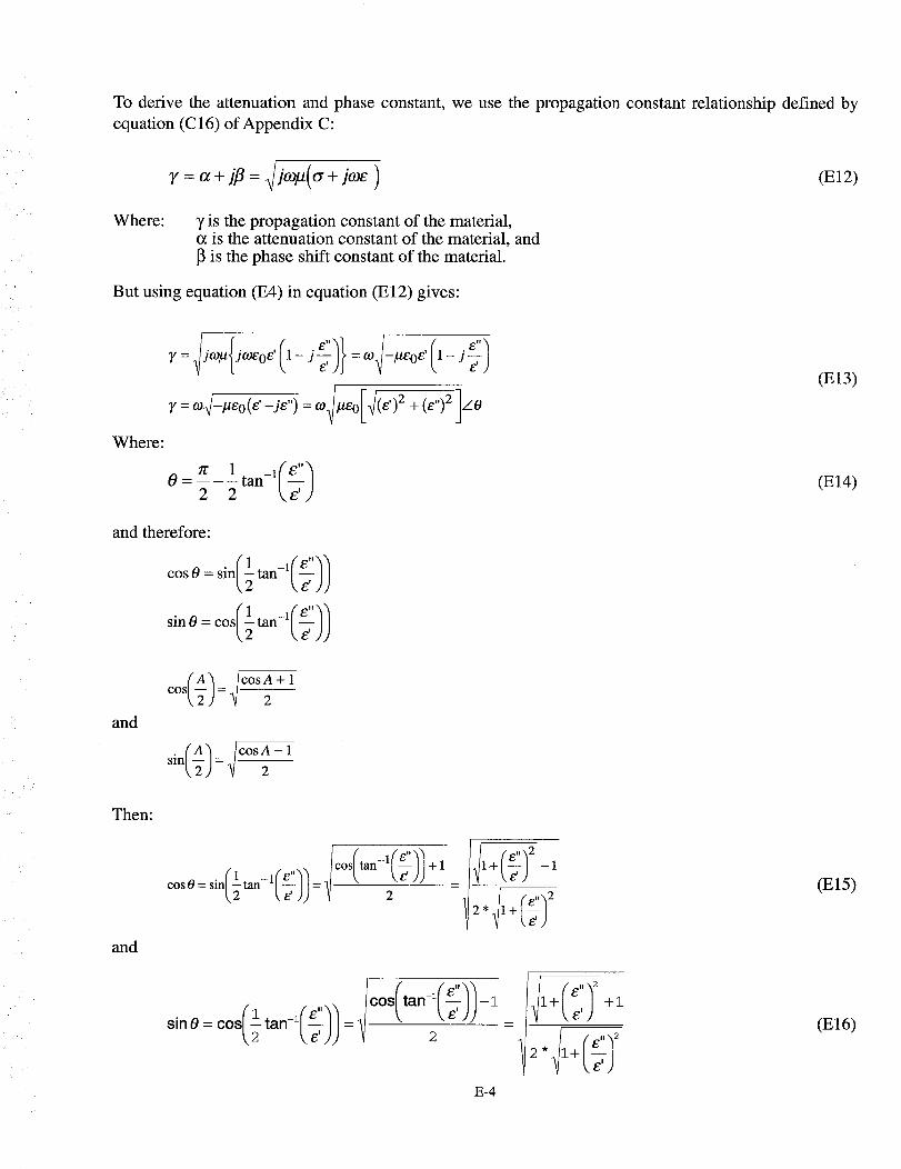
To derive the attenuation and phase constant, we use the propagation constant relationship defined by
equation (C16) of Appendix C:
Where: 7 is the propagation constant of the material,is the attenuation constant of the material, andis the phase shift constant of the material.
But using equation (E4) in equation (El2) gives:
(El2)
,'L
Where:
r= jo,_,jo,=o=,(1-jT);=o,-.=oe =';_
r=o_4-#eo(e'-je") =o_II_eo[4(e')2 + (e")2 Jzo
__
and therefore:
cosO= sin(ltan-l('_,'))
sin0 = cos(l- tan-'(e"_\2 \e' )J
and
co(A)=_'
./--_)=?°sA-_
(El3)
(E14)
Then:
and
(1 (,_))cost._,cos 0 = sin tan-1 = e
gl fe"'_'_ cos(tan _,'))-1= /__1+_)
sinl=c°s_-2tan-1_-g:_= 1 I
E-4
(El5)
(El6)

Theattenuationconstantis therealpartof thewaveimpedance,thus:
giving:
_=l_lcos0=,o _0_/(_')2+(_")2 sio tan-l_,;J
The phase constant is the imaginary part of the wave impedance, thus:
]_= I1'1sin 0 = w#bte° #(g)2 + (e")2 [c°s/1 tan-1 '{/]
Resulting in:
j j IJ_=_. /_eOg 1+(_")2 12*llkE'']l+(f) 2+1
-¢01_-Ill +/_,'/2 +1]
(El7)
(El8)
Equations (E6), (El0), (Ell), (E17), and (El8) provide the necessary RF characteristics for the cover sheetfrom the measured complex dielectric constant.
E-5

REPORT DOCUMENTATION PAGEJ Form ApprovedOMB No. 0704-0188
Public reporting burden for this collection of information is estimated to average 1 hour per response, including the time for reviewing instructions, searching existing data sources,
gathering and maintaining the data needed, and completing and reviewing the collection of information. Send comments regarding this burden estimate or any other aspect of this
collection of information, including suggestions for reducing this burden, to Washington Headquarters Services, Directorate for Information Operations and Reports, 1215 Jefferson
Davis Highway, Suite 1204, Arlington, VA 22202-4302, and to the Office of Management and Budget, Paperwork Reduction Project (0704-0188), Washington, DC 20503.
1. AGENCY USE ONLY (Leave blank) 2. REPORT DATE 3. REPORT TYPE AND DATES COVERED
May 1997 Technical Memorandum4. TITLE AND SUBTITLE 5. FUNDING NUMBERS
Technique for Predicting the Radio Frequency Field StrengthInside an Enclosure
6. AUTHOR(S)
Michael P. Hallett and Jerry P. Reddell
7. PERFORMING ORGANIZATION NAME(S) AND ADDRESS (ES)
Goddard Space Flight Center
Greenbelt, Maryland 20771
9. SPONSORING / MONITORING AGENCY NAME(S) AND ADDRESS (ES)
National Aeronautics and Space Administration
Washington, DC 20546-0001
C-NAS5-30722
Code 470
8. PEFORMING ORGANIZATIONREPORT NUMBER
97B00038
10, SPONSORING/MONITORINGAGENCY REPORT NUMBER
NASA TM- 104646
11. SUPPLEMENTARY NOTES
Hallett: Goddard Space Flight Center, Greenbelt, Maryland;
Reddell: McDonnell Douglas, Seabrook, Maryland.
12a. DISTRIBUTION / AVAILABILITY STATEMENT
Unclassified - Unlimited
Subject Category 33
Availability: NASA CASI (301) 621-0390.
12b. DISTRIBUTION CODE
13. ABSTRACT (Maximum 200 words)
This technical memo represents a simple analytical technique for predicting the radio frequency (RF)
field inside an enclosed volume in which radio frequency occurs. The technique was developed to
predict the RF field strength within a launch vehicle fairing in which some payloads desire to launch
with their telemetry transmitter radiating. This technique considers both the launch vehicle and the
payload aspects.
14. SUBJECT TERMS
RF, radio frequency, fairing, payload, launch vehicle
17. SECURITY CLASSIFICATION
OF REPORT
Unclassified
NSN 7540-01-280-5500
18. SECURITY CLASSIFICATION
OF THIS PAGE
Unclassified
19. SECURITY CLASSIFICATIONOF ABSTRACT
Unclassified
15. NUMBER OF PAGES
8416. PRICE CODE
20. LIMITATION OF ABSTRACT
UL
Standard Form 298 (Rev. 2-89)Prescribed by ANSI Std. Z39.18
298-102