technique for measuring the coefficient of restitution … · technique for measuring the...
TRANSCRIPT

Technique for Measuring the Coefficient of Restitution for Microparticle Sand Impacts at
High Temperature for Turbomachinery Applications
Colin James Reagle
Dissertation submitted to the faculty of the Virginia Polytechnic Institute and State University in
partial fulfillment of the requirements for the degree of
Doctor of Philosophy
In
Mechanical Engineering
Wing F. Ng
Srinath V. Ekkad
Danesh K. Tafti
Clinton L. Dancey
Muhammad R. Hajj
August 22, 2012
Blacksburg, Virginia, USA
Keywords: Microparticle, Coefficient of Restitution, Turbomachinery, Impact
Copyright 2012

Technique for Measuring the Coefficient of Restitution for Microparticle Sand
Impacts at High Temperature for Turbomachinery Applications
Colin James Reagle
Abstract
Erosion and deposition in gas turbine engines are functions of particle/wall interactions
and the Coefficient of Restitution (COR) is a fundamental property of these interactions. COR
depends on impact velocity, angle of impact, temperature, particle composition, and wall
material. In the first study, a novel Particle Tracking Velocimetry (PTV) / Computational Fluid
Dynamics (CFD) hybrid method for measuring COR has been developed which is simple, cost-
effective, and robust. A Laser-Camera system is used in the Virginia Tech Aerothermal Rig to
measure microparticles velocity. The method solves for particle impact velocity at the surface by
numerical methods. The methodology presented here characterizes a difficult problem by a
combination of established techniques, PTV and CFD, which have not been used in this capacity
before. The current study characterizes the fundamental behavior of sand at different impact
angles. Two sizes of Arizona Road Dust (ARD) and one size of Glass beads are impacted on to
304-Stainless Steel. The particles are entrained into a free jet of 27m/s at room temperature.
Mean results compare favorably with trends established in literature. This technique to measure
COR of microparticle sand will help develop a computational model and serve as a baseline for
further measurements at elevated, engine representative air and wall temperatures.
In the second study, ARD is injected into a hot flow field at temperatures of 533oK,
866oK, and 1073
oK to measure the effects of high temperature on particle rebound. The results
are compared with baseline measurements at ambient temperature made in the VT Aerothermal
Rig, as well as previously published literature. The effects of increasing temperature and velocity
led to a 12% average reduction in total COR at 533oK (47m/s), a 15% average reduction at
866oK (77m/s), and a 16% average reduction at 1073
oK (102m/s) compared with ambient results.
From these results it is shown that a power law relationship may not conclusively fit the COR vs
temperature/velocity trend at oblique angles of impact. The decrease in COR appeared to be
almost entirely a result of increased velocity that resulted from heating the flow.

iii
Acknowledgements
First and foremost I need to thank my Mom Paulette, Dad Bill, and sister Jesy for their
emotional and financial support over the past five years. It certainly wouldn’t have been possible
to achieve my goals without them. To my co-advisors Dr. Ng and Dr. Ekkad, I have the greatest
respect for them as mentors. I’ve been incredibly lucky to have spent these last five years
learning from such a well-balanced pair. If my parents have been my personal role models, they
have certainly been my professional ones. To the rest of my committee, Dr. Tafti, Dr. Dancey,
and Dr. Hajj, I thank you for your support and interest in my work. I would like to thank Song
Xue for sharing an office with me the last 3 plus years, administering sanity checks, and a
providing a general perspective about the world. To Jacob Delimont and Sukhjinder Singh, I
thank you or all of the long hours and thoughtful discussion on this project as it has developed
over the past 3 years. Mike Fertall deserves special thanks for his help getting the rig up and
running as well as all advice aquarium related. Avi Friedman deserve acknowledgement for
faithfully helping to run experiments. I’d like to thank Diana Israel for personally placing over
250 separate orders related to this project and always doing it with kind words and a smile on her
face. The entire ME Staff of Melissa Williams, Cathy Hill, Jackie Woodyard, Brandy McCoy,
Mandy McGlothlin,, Ross Verbrugge, Matt Swift, Ben Poe and Jamie Archual for a variety of
reasons. If I didn’t have to write this dissertation I’d consider trying to list them all. To the guys
in the shop, James, Bill, Tim, Phil and Johnny, I appreciate all of the advice, odd jobs and formal
ones that kept this project moving.
The work detailed here would not be possible without the support and direction of Rolls-
Royce, especially Veera Rajendran, Steve Gegg, Mark Creason, N. Wagers, H. Kwen, and B.
Barker.
Finally, thank you to my small family, Ella, Joey and Allie. Without you guys to come
home to, I think I would be a bit batty at this point. Thank you for keeping things in perspective
through this long process and reminding me daily what is truly important in life. I love you and
appreciate you every day.

iv
Preface
This dissertation is organized in a manuscript format that includes two individual papers
directly related to the Ph.D. dissertation contained within. The author was involved in all aspects
of the experiment from modifying the building, designing the rig hardware, conducting the
experiments, reducing the data, and analyzing the results. Many elements beyond the two papers
are presented in the Appendix of the dissertation. These appendices provide additional
information related to the experimental technique and results.
The first paper contains the ambient experimental data that was used to verify the hybrid
Particle Tracking Velocimetry (PTV) / Computational Fluid Dynamics (CFD) technique used in
the VT Aerothermal Rig. The paper is currently being submitted for journal publication after the
initial work was presented to ASME-IGTI Turbo Expo 2012. The experimental and data
reduction techniques are explained in detail and appropriate comparisons are made with literature
to validate the experiment. The paper presents data for 3 different particles, though the main
focus is on the Arizona Road Dust (ARD) 20-40μm particles as they will be used exclusively in
the second paper. The main contribution of the first paper is in explaining the technique and
validating the ambient temperature results that it produced.
Some key literature that represents the previous state of the art for measuring COR is
discussed here. Tabakoff et al. [1] was one of the first researchers to present COR data for
microparticle quartz at different impact angles using a strobe photography method. Erosion was
also measured. This method was limited to large particles and involved the time consuming
reduction of measuring streaks and particle movement between images. Much of the COR work
conducted at the University of Cincinnati was transitioned to a Laser Doppler Velocimetry
method where Tabakoff [2] presented results for 15μm fly ash impacting a variety of aerospace
materials. While LDV can provide good measurements very close to the impact surface, it is
tedious to setup and only provides point measurements. Wall et al. [3] presented results for
microparticles less than 10μm impacting a variety of surfaces at 90o
from 1-100 m/s using LDV.
Over 250 impact events were measured for each test case. Wall et al. also utilized a 1-D velocity
correction method in which particles with very small Stokes number were used to correct for
velocity changes of large particles between measurement location and the impact surface.
The experimental technique discussed in detail in this dissertation is superior in a number
of ways to the previous mentioned techniques. The setup is relatively simple and does not need
v
change for different impact angles. All of the ambient temperature data can be captured in less
than a day. Reducing the data takes approximately one more day. This streamlined process that
was developed allows for rapid iteration of target materials. A large number of impacts are also
captured at a range of angles, the ambient data presented has over 13,000 impacts from 19-84o.
The necessary measurement equipment is found in any off the shelf PIV measurement system
and all of the codes are open source.
The second paper details the heated Coefficient of Restitution (COR) experiments that
were conducted in the VT Aerothermal Rig. Measuring COR at high temperature was the central
motivation of developing and validating the experimental technique discussed in the first paper.
The experiments were conducted at 533oK, 866
oK, and 1073
oK in an attempt to capture a change
in rebound behavior leading up to deposition, considered COR = 0 in this work.
Some of the key published works are presented in this preface. Johnson [4] presented
metal on metal impacts for large spheres with increasing velocity. The COR of a steel ball
impacting bronze, brass, or lead was shown to be proportional to ⁄ . Mok and Duffy [5]
presented COR for normal impacts at velocities up to 5m/s. Results for a 1in steel ball impacting
a lead and aluminum surface were shown at temperatures of ambient, approximately ½ Tmelt, and
¾ Tmelt of the surface material. Results were essentially unchanged for the lead specimen. At
900oF the aluminum specimen showed a reduction of approximately 0.08 over ambient. This
was essentially constant from 1m/s to 5m/s, the regions where plastic deformation dominated.
Brenner et al. [6] also measured impacts at high temperature. COR data was presented for
normal impacts of iron balls, approximately 120μm in diameter, impacting an Al2O3 coated iron
surface. Results presented at 1073oK were shown to decrease with the term ⁄ . Similar
reductions in COR vs Velocity were observed for data taken at 973oK and 1073
oK up to 2 m/s.
The data presented in the second paper has two key contributions to published literature.
First, it presents oblique COR data at high temperature. Second, the particles are of engine
representative (i.e. size, velocity and composition). These results are of significance because
particles ingested into an engine are typically very small. These particles will try to follow the
flow and rarely impact at 90o angles. The temperatures tested are representative of secondary
flows in the internal cooling passages of a gas turbine. An overall correlation for COR of
different materials, velocity and impact angles does not exist in published literature so empirical
data at engine representative conditions will give the most accurate results. The results can be

vi
used to accurately model particle transport after impact through engine realistic geometries using
CFD. This can lead to better prediction of the effects of erosion and deposition on engine
hardware by accurately predicting the location of subsequent impacts, after the initial impact.
[1] Tabakoff, W., Grant, G., and Ball, R., 1974, "An Experimental Investigation of Certain
Aerodynamic Effects on Erosion," AIAA-74-639.
[2] Tabakoff, W., 1991, "Measurements of Particles Rebound Characteristics on Materials Used
in Gas Turbines," J. of Propulsion and Power, 7(5), pp. 805-813.
[3] Wall, S., John, W., Wang H.C., and Goren, S. L., 1990, "Measurements of Kinetic Energy
Loss for Particles Impacting Surfaces," Aerosol Science and Technology, 12, pp. 926-946.
[4] Johnson, K. L., 1985, Contact Mechanics, Cambridge University Press, Cambridge, UK.
[5] Mok, C. H., and Duffy, J., 1964, "THE BEHAVIOUR OF METALS AT ELEVATED
TEMPERATURES UNDER IMPACT WITH A BOUNCING BALL," Int J Mech Sci, 6, pp.
161-175.
[6] Brenner, S. S., Wriedt, H. A., and Oriani, R. A., 1981, "Impact adhesion of iron at elevated
temperatures," Wear, 68(2), pp. 169-190.
vii
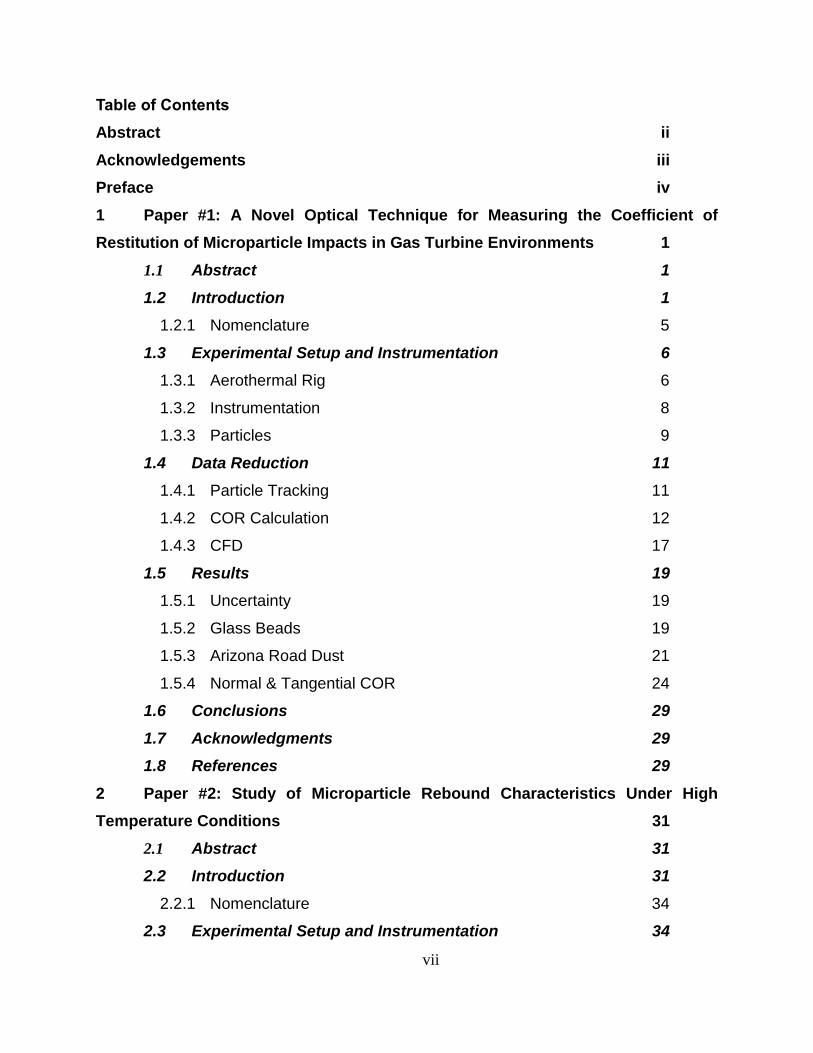
Table of Contents
Abstract ii
Acknowledgements iii
Preface iv
1 Paper #1: A Novel Optical Technique for Measuring the Coefficient of
Restitution of Microparticle Impacts in Gas Turbine Environments 1
1.1 Abstract 1
1.2 Introduction 1
1.2.1 Nomenclature 5
1.3 Experimental Setup and Instrumentation 6
1.3.1 Aerothermal Rig 6
1.3.2 Instrumentation 8
1.3.3 Particles 9
1.4 Data Reduction 11
1.4.1 Particle Tracking 11
1.4.2 COR Calculation 12
1.4.3 CFD 17
1.5 Results 19
1.5.1 Uncertainty 19
1.5.2 Glass Beads 19
1.5.3 Arizona Road Dust 21
1.5.4 Normal & Tangential COR 24
1.6 Conclusions 29
1.7 Acknowledgments 29
1.8 References 29
2 Paper #2: Study of Microparticle Rebound Characteristics Under High
Temperature Conditions 31
2.1 Abstract 31
2.2 Introduction 31
2.2.1 Nomenclature 34
2.3 Experimental Setup and Instrumentation 34

viii
2.3.1 Aerothermal Rig 34
2.3.2 Instrumentation 36
2.3.3 Test Conditions and Material Properties 38
2.4 Data Reduction 40
2.5 Results 41
2.5.1 Uncertainty 41
2.5.2 Total Coefficient of Restitution 42
2.5.3 Normal Coefficient of Restitution 43
2.5.4 Tangential Coefficient of Restitution 44
2.6 Discussion on Temperature/Velocity Effects 46
2.7 Conclusions 52
2.8 Acknowledgments 53
2.9 References 53
Conclusions and Future Work 55
A. APPENDIX: Two Pass Channel 57
B. APPENDIX: Gravity Fed Shakedown Testing and Observations 60
Incoming/Rebounding particles in VT Aerothermal Rig 61
Double Bounce in VT Aerothermal Rig 62
C. APPENDIX: Sensitivity and Uncertainty 65
D. APPENDIX: Particle Delivery System 68
E. APPENDIX: Traverse Design 71
F. APPENDIX: Rig Modifications and Modernization 75
Building Modifications 75
Rig Controls 76
Flowpath Hardware 78
Cooling Tower 79
G. APPENDIX: COR Data Reduction Code 84
Post Processing PTV txt files 84
Post Processing Results File 102
ix
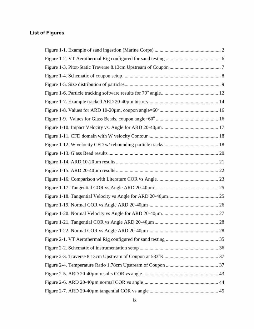
List of Figures
Figure 1-1. Example of sand ingestion (Marine Corps) ..................................................... 2
Figure 1-2. VT Aerothermal Rig configured for sand testing ............................................ 6
Figure 1-3. Pitot-Static Traverse 8.13cm Upstream of Coupon ......................................... 7
Figure 1-4. Schematic of coupon setup............................................................................... 8
Figure 1-5. Size distribution of particles............................................................................. 9
Figure 1-6. Particle tracking software results for 70o angle.............................................. 12
Figure 1-7. Example tracked ARD 20-40µm history ....................................................... 14
Figure 1-8. Values for ARD 10-20µm, coupon angle=60o ............................................... 16
Figure 1-9. Values for Glass Beads, coupon angle=60o .................................................. 16
Figure 1-10. Impact Velocity vs. Angle for ARD 20-40μm ............................................. 17
Figure 1-11. CFD domain with W velocity Contour ........................................................ 18
Figure 1-12. W velocity CFD w/ rebounding particle tracks ............................................ 18
Figure 1-13. Glass Bead results ........................................................................................ 20
Figure 1-14. ARD 10-20µm results .................................................................................. 21
Figure 1-15. ARD 20-40µm results .................................................................................. 22
Figure 1-16. Comparison with Literature COR vs Angle ................................................. 23
Figure 1-17. Tangential COR vs Angle ARD 20-40μm ................................................... 25
Figure 1-18. Tangential Velocity vs Angle for ARD 20-40μm ........................................ 25
Figure 1-19. Normal COR vs Angle ARD 20-40μm ........................................................ 26
Figure 1-20. Normal Velocity vs Angle for ARD 20-40μm ............................................. 27
Figure 1-21. Tangential COR vs Angle ARD 20-40μm ................................................... 28
Figure 1-22. Normal COR vs Angle ARD 20-40μm ........................................................ 28
Figure 2-1. VT Aerothermal Rig configured for sand testing .......................................... 35
Figure 2-2. Schematic of instrumentation setup ............................................................... 36
Figure 2-3. Traverse 8.13cm Upstream of Coupon at 533oK ........................................... 37
Figure 2-4. Temperature Ratio 1.78cm Upstream of Coupon .......................................... 37
Figure 2-5. ARD 20-40µm results COR vs angle ............................................................. 43
Figure 2-6. ARD 20-40µm normal COR vs angle ............................................................ 44
Figure 2-7. ARD 20-40µm tangential COR vs angle ....................................................... 45

x
Figure 2-8. ARD 20-40µm COR vs Velocity ................................................................... 48
Figure 2-9. Normal COR vs Normal Impact Velocity ...................................................... 50
Figure 2-10. Tangential COR vs Tangential Impact Velocity .......................................... 51
Figure 2-11. ARD 20-40µm COR vs KE (½mv2) ........................................................... 52
Figure A-1. Two Pass Channel Geometry ........................................................................ 57
Figure A-2. Two pass channel experimental setup ........................................................... 58
Figure A-3. Tape attached on endwalls, underneath ribs.................................................. 58
Figure A-4. Results of the 2 pass channel near the turn ................................................... 59
Figure B-1. Shakedown testing experimental setup ......................................................... 60
Figure B-2. Particle tracks and classification from Shakedown testing ........................... 61
Figure B-3. Incoming/Rebounding Characterization ........................................................ 62
Figure B-4. Incoming Velocity Histogram, coupon angle=80o ........................................ 63
Figure B-5. Double Bounce Tracks .................................................................................. 63
Figure C-1. Ambient Sensitivity to CFD Data................................................................. 65
Figure C-2. Sensitivity to CFD for 60o and 80
o coupon angle ......................................... 66
Figure C-3. Curve fitting, local, and global averaging .................................................... 67
Figure D-1. Remote Particle Delivery System ................................................................. 70
Figure E-1. Traverse Schematic with Pitot-Static Probe .................................................. 72
Figure E-2. Laser-Camera image of TC Probe in front of coupon ................................... 74
Figure F-1. Rig Components Delivered to Airport Lab .................................................... 75
Figure F-2. Rig prior to running at high temperature ....................................................... 76
Figure F-3. Labview/Operator Interface ........................................................................... 77
Figure F-4. Custom Coupon Flange.................................................................................. 79
Figure F-5. Burner temperatures during HTC test with static water ................................ 80
Figure F-6. Cooling Tower and Rig Exhaust ................................................................... 81
Figure F-7. Electrical Components Added for Cooling Circuit ........................................ 82
Figure F-8. Instrumentation Cooling Setup ...................................................................... 83
xi
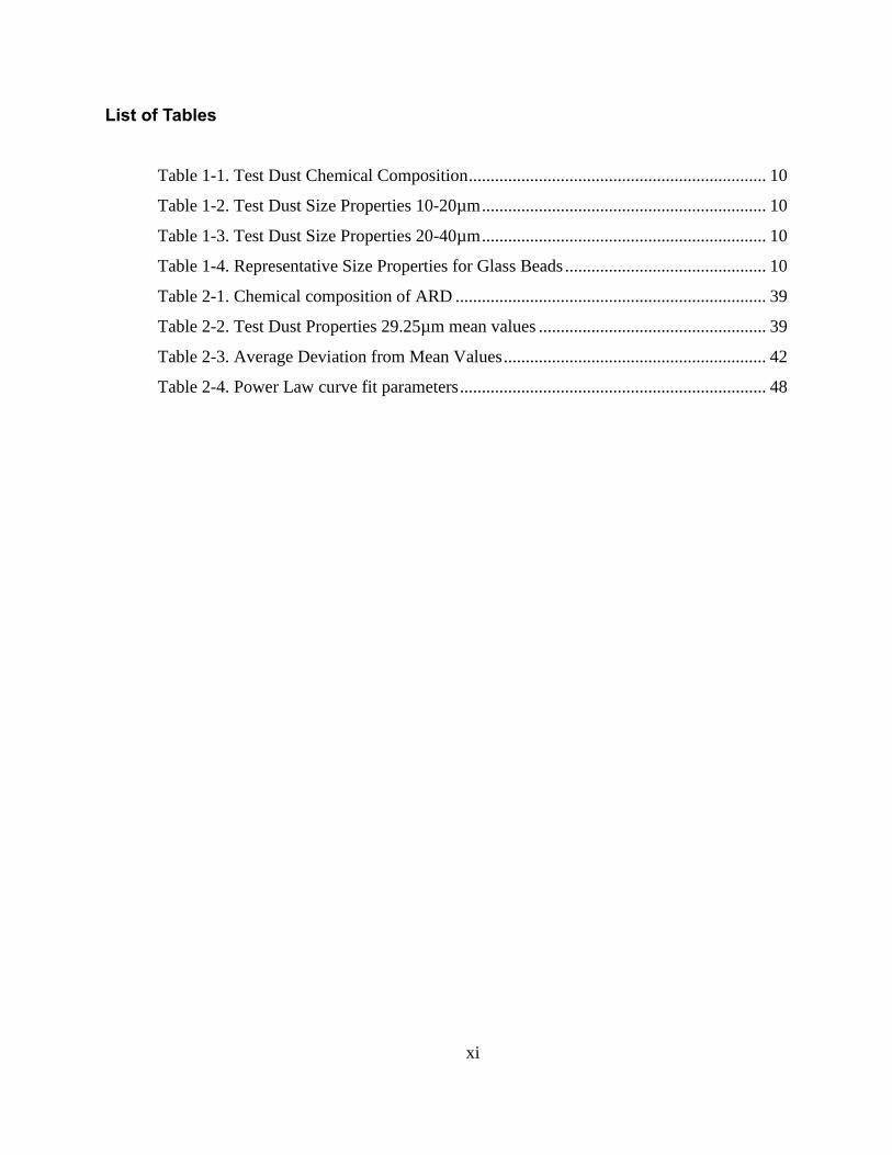
List of Tables
Table 1-1. Test Dust Chemical Composition .................................................................... 10
Table 1-2. Test Dust Size Properties 10-20µm ................................................................. 10
Table 1-3. Test Dust Size Properties 20-40µm ................................................................. 10
Table 1-4. Representative Size Properties for Glass Beads .............................................. 10
Table 2-1. Chemical composition of ARD ....................................................................... 39
Table 2-2. Test Dust Properties 29.25µm mean values .................................................... 39
Table 2-3. Average Deviation from Mean Values ............................................................ 42
Table 2-4. Power Law curve fit parameters ...................................................................... 48
1
1 Paper #1: A Novel Optical Technique for Measuring the Coefficient of
Restitution of Microparticle Impacts in Gas Turbine Environments
1.1 Abstract
Erosion and deposition in gas turbine engines are functions of particle/wall interactions
and the Coefficient of Restitution (COR) is a fundamental property of these interactions. COR
depends on impact velocity, angle of impact, temperature, particle composition, and wall
material. A novel Particle Tracking Velocimetry (PTV) / Computational Fluid Dynamics (CFD)
hybrid method for measuring COR has been developed which is simple, cost-effective, and
robust. A Laser-Camera system is used in the Virginia Tech Aerothermal Rig to measure
velocity trajectories of microparticles. The method solves for particle impact velocity at the
impact surface by numerical methods. The methodology presented here attempts to characterize
a difficult problem by a combination of established techniques, PTV and CFD, which have not
been used in this capacity before. The current study attempts to characterize the fundamental
behavior of sand at different impact angles. Two sizes of Arizona Test Dust and one size of
Glass beads are impacted on to a 304-Stainless Steel coupon. The particles are entrained into a
free jet of 27m/s at room temperature. Impact angle was varied from almost 90 to 25 degrees
depending on particle. Mean results compare favorably with trends established in literature.
The utilization of this technique to measure COR of microparticle sand will help develop a
computational model and serve as a baseline for further measurements at elevated, engine
representative air and wall temperatures.
1.2 Introduction
In recent years, gas turbines operating around the world have been exposed to high levels
of particulates. Aircraft operating at low altitudes or at remote landing field are commonly
subject to large amounts of particle ingestion, examples of the amount of sand that can be
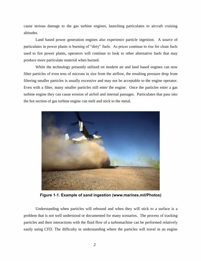
ingested into a gas turbine engine can be seen in Figure 1-1. This is particularly true of desert
environments. A gas turbine engine will be exposed to significant amounts of sand, dust, and
particulate, even while operating from a fully modern airfield in a desert environment. Many
natural disasters also contribute to the amount of particulates in the air. Large dust storms also
2
cause serious damage to the gas turbine engines, launching particulates to aircraft cruising
altitudes.
Land based power generation engines also experience particle ingestion. A source of
particulates in power plants is burning of “dirty” fuels. As prices continue to rise for clean fuels
used to fire power plants, operators will continue to look to other alternative fuels that may
produce more particulate material when burned.
While the technology presently utilized on modern air and land based engines can now
filter particles of even tens of microns in size from the airflow, the resulting pressure drop from
filtering smaller particles is usually excessive and may not be acceptable to the engine operator.
Even with a filter, many smaller particles still enter the engine. Once the particles enter a gas
turbine engine they can cause erosion of airfoil and internal passages. Particulates that pass into
the hot section of gas turbine engine can melt and stick to the metal.
Figure 1-1. Example of sand ingestion (www.marines.mil/Photos)
Understanding when particles will rebound and when they will stick to a surface is a
problem that is not well understood or documented for many scenarios. The process of tracking
particles and their interactions with the fluid flow of a turbomachine can be performed relatively
easily using CFD. The difficulty in understanding where the particles will travel in an engine
3
comes from modeling the interaction between the particle and the solid surfaces of the engine.
This aspect of a particle’s journey through a gas turbine engine has been the subject of a great
deal of research throughout the years.
The theory of colliding solids has been around since Heinrich Hertz fathered the field of
contact mechanics by combining classical elasticity theory with continuum mechanics [1]. Hertz
theory has been widely applied as the basis of solutions for stress, compression, time, and
separation of impacting solids. Since then, numerous researchers have proposed improvements
to account for phenomenon, such as plastic deformation, associated with colliding solids. With
the introduction of plastic deformation to Hertzian theory, approximations can be made for
coefficient of restitution of real particles at higher impacting velocities. The contact is broken up
into an elastic compression, plastic deformation, and restitution of stored elastic strain energy.
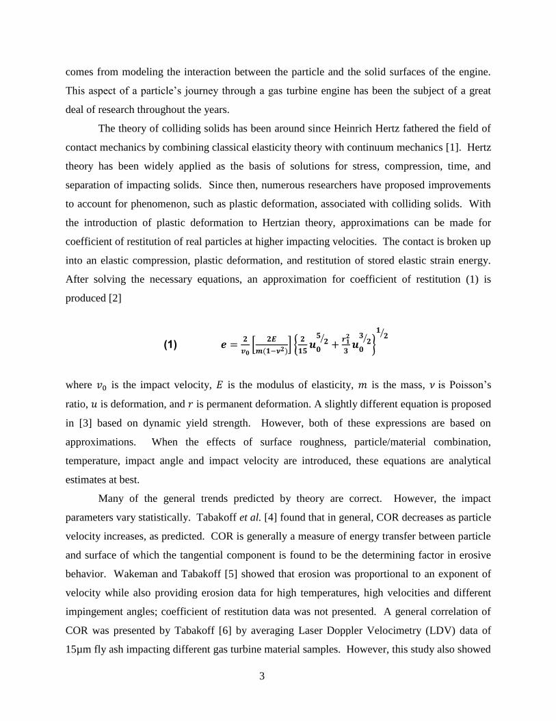
After solving the necessary equations, an approximation for coefficient of restitution (1) is
produced [2]
(1) 𝒆 =𝟐
𝒗𝟎[
𝟐𝑬
𝒎(𝟏 𝝂𝟐)] {
𝟐
𝟏𝟓𝒖𝟎
𝟓𝟐⁄ +
𝒓𝟏𝟐
𝟑𝒖𝟎
𝟑𝟐⁄ }
𝟏𝟐⁄
where is the impact velocity, is the modulus of elasticity, is the mass, is Poisson’s
ratio, is deformation, and is permanent deformation. A slightly different equation is proposed
in [3] based on dynamic yield strength. However, both of these expressions are based on
approximations. When the effects of surface roughness, particle/material combination,
temperature, impact angle and impact velocity are introduced, these equations are analytical
estimates at best.
Many of the general trends predicted by theory are correct. However, the impact
parameters vary statistically. Tabakoff et al. [4] found that in general, COR decreases as particle
velocity increases, as predicted. COR is generally a measure of energy transfer between particle
and surface of which the tangential component is found to be the determining factor in erosive
behavior. Wakeman and Tabakoff [5] showed that erosion was proportional to an exponent of
velocity while also providing erosion data for high temperatures, high velocities and different
impingement angles; coefficient of restitution data was not presented. A general correlation of
COR was presented by Tabakoff [6] by averaging Laser Doppler Velocimetry (LDV) data of
15µm fly ash impacting different gas turbine material samples. However, this study also showed
4
the percent difference in mean COR was higher than 25% for different materials. This shows a
distinct effect of impacting particle/material combination on rebound characteristics. Tabakoff et
al. [7] later went on to repeat many of these same experiments using 100-200μm sand particles
impacting aerospace materials. Comparing the mean results led to a notable difference in COR
values compared with the fly ash particles.
While tangential and normal COR have been presented, out of plane measurements made
by Eroglu and Tabakoff [8] found that out of plane COR was insensitive to changes in impact
angle. Sommerfeld and Huber [9] experimented with 100µm and 500µm glass beads and non-
spherical quartz particles on smooth and rough surfaces. Surface roughness and particle
roundness were shown to have similar effects on COR and rebound angles. The rebound angle
was often larger than the impact angle; this effect was termed the shadow effect.
In documented literature, no data exists for COR of microparticle sand impacting at
different angles, velocities, or materials. These factors all play a notable role in mean COR as
well as deviation in the empirical data. The current work presents COR data for microparticle
sand impacting stainless steel at ambient temperature for one velocity. This is important because
upon entering the turbine inlet, the particle must go through a very complex flowfield before it
can be ejected out of the exhaust. During this trip through the engine the particle is very likely to
come in contact with a surface. Only representative data for COR can accurately predict the
particles trajectory after a single impact. Each subsequent collision, with different impact
conditions, will change the particle’s course and determine the next collision surface. The
location and intensity of these collisions can drastically affect the performance and life of a turbo
machine, thus accurate impact modeling based on realistic data must be incorporated into the
particle transport physics.
The technique utilized in the current work is of importance as well as it allows for COR
measurements in 2-D forced flowfield. In reported literature, high speed imaging [4] and LDV
[6-9] are the two main methods of measuring COR. High speed imaging has its limitations with
respect to particle size and LDV while providing high quality data, requires precise setup and
seeding for a single point measurement. LDV becomes even more difficult to set up when the
effects of thermal expansion must also be accounted for. Wall et. al. [10] utilized an LDV
system and calculated a 1-D velocity correction based on tracer particle measurements. While
Laser-Camera measurements are not possible in the near wall region of a flow, the 2-D flowfield

5
correction described below can still extract quality data at a range of angles while still being
relatively simple to setup. A novel method of Particle Velocimetry Tracking (PTV) imaging and
particle tracking using a CFD simulated flowfield is presented. The technique can be applied at
high temperatures, different velocities, and with different particle/material combinations utilizing
economical hardware and software.
1.2.1 Nomenclature
acceleration
Drag Coefficient
diameter
Coefficient of Restitution (COR)
Modulus of elasticity
Drag force
length
mass
radius of permanent deformation
Stokes Number
time
deformation
Velocity
β impact angle
ν Poisson’s ratio
ρ density
subscript
n normal
p particle
t tangential
∞ freestream
6
1.3 Experimental Setup and Instrumentation
1.3.1 Aerothermal Rig
Virginia Tech Aerothermal Rig was donated to Virginia Tech by Rolls-Royce in
September 2010. This rig was used in previous heat transfer studies conducted at their facility in
Indianapolis, IN. Hylton et al. [11] used the same facility to conduct a series of tests on shower
head and film cooling heat transfer at a temperature of 700K. Nealy et al. [12] used the rig at
temperatures of 811K to measure heat transfer on nozzle guide vanes at different transonic Mach
numbers. The operational specifications for this rig when installed in Indianapolis were reported
as 2.2kg/s at a maximum of 16atm and 2033K by Rolls-Royce.
At Virginia Tech the pressure and temperature capabilities for this rig are being brought
up gradually in steps as the rig is fully recomissioned. For the present study the Aerothermal Rig
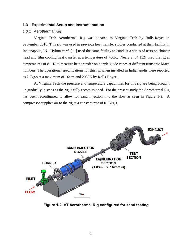
has been reconfigured to allow for sand injection into the flow as seen in Figure 1-2. A
compressor supplies air to the rig at a constant rate of 0.15kg/s.
Figure 1-2. VT Aerothermal Rig configured for sand testing
7
The flow is regulated upstream with a 10.2cm globe valve. The air then passes through a
sudden expansion burner capable of heating the flow. The burner is not used to heat the flow in
the current study.
At the exit downstream of the burner, the cross-section of the flow is reduced in diameter
from 30.5cm to 7.62cm. During the contraction section, the test particles are injected into the
mainstream flow. The particles are entrained in a compressed air flow that has been bled from
the main compressor upstream of the burner. The particles then enter a 1.83m long, 7.62cm
diameter equilibration tube which enables particles of various sizes to accelerate to the same
speed (and temperature) as the rest of the flow. The flow exits the equilibration tube as a free jet
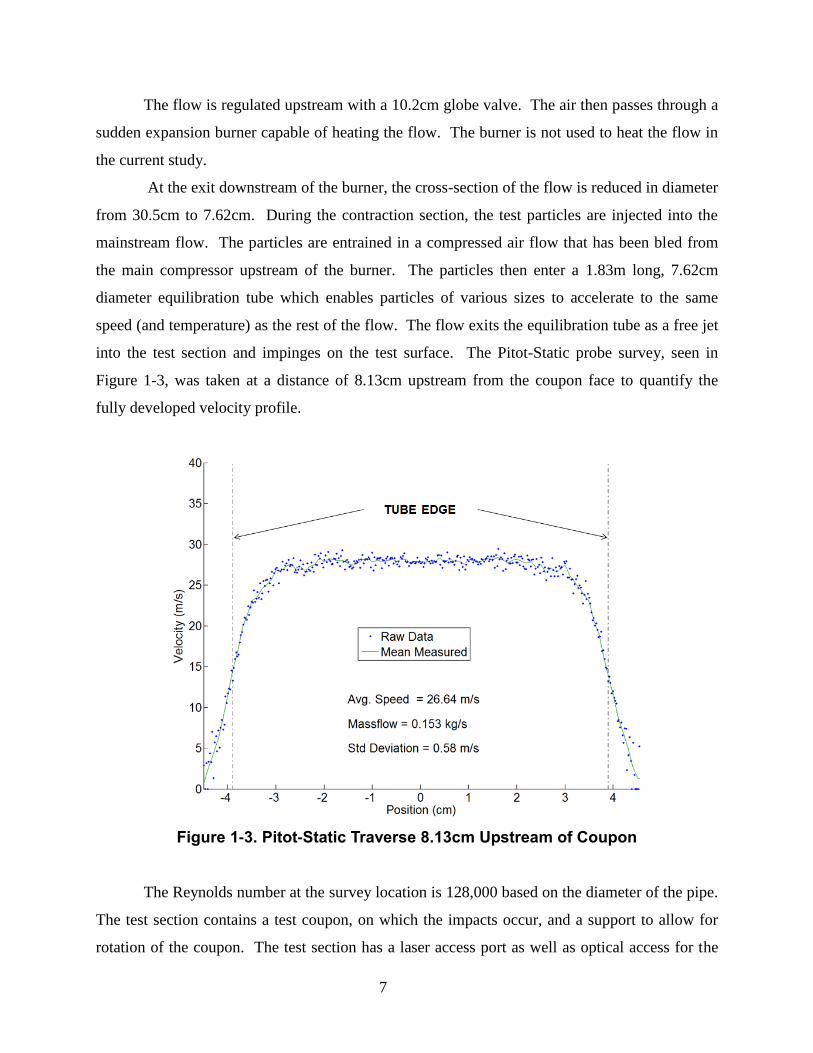
into the test section and impinges on the test surface. The Pitot-Static probe survey, seen in
Figure 1-3, was taken at a distance of 8.13cm upstream from the coupon face to quantify the
fully developed velocity profile.
Figure 1-3. Pitot-Static Traverse 8.13cm Upstream of Coupon
The Reynolds number at the survey location is 128,000 based on the diameter of the pipe.
The test section contains a test coupon, on which the impacts occur, and a support to allow for
rotation of the coupon. The test section has a laser access port as well as optical access for the
8
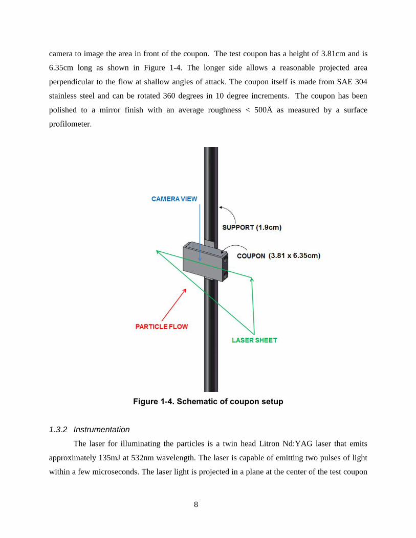
camera to image the area in front of the coupon. The test coupon has a height of 3.81cm and is
6.35cm long as shown in Figure 1-4. The longer side allows a reasonable projected area
perpendicular to the flow at shallow angles of attack. The coupon itself is made from SAE 304
stainless steel and can be rotated 360 degrees in 10 degree increments. The coupon has been
polished to a mirror finish with an average roughness < 500Å as measured by a surface
profilometer.
Figure 1-4. Schematic of coupon setup
1.3.2 Instrumentation
The laser for illuminating the particles is a twin head Litron Nd:YAG laser that emits
approximately 135mJ at 532nm wavelength. The laser is capable of emitting two pulses of light
within a few microseconds. The laser light is projected in a plane at the center of the test coupon
9
as shown in Figure 1-4. A Dantec Dynamics® FlowSense camera equipped with a Zeiss®
Makro-Planar 2/50 lens is used to capture the particle images at 2048x2048 resolution. Both the
laser and the camera are synced by a timer box ensuring illumination and imaging occur
concurrently.
1.3.3 Particles
The sand particles used were Arizona Test Dust. Intermediate Grades of Nominal 10-
20µm and also Nominal 20-40 µm were tested in this experiment. Arizona road dust (ARD) has
been widely used as a standard test dust for filtration, automotive and heavy equipment testing.
It is also an excellent choice for studying sand ingestion in jet engines as it is has very similar
properties to sands found throughout the world and is readily available. Glass beads with large
Stokes # were also tested in this experiment to verify the technique for a controlled case. This
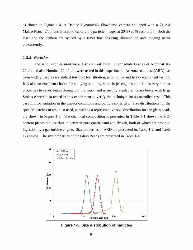
case limited variation in the impact conditions and particle sphericity. Size distributions for the
specific batches of test dust used, as well as a representative size distribution for the glass beads
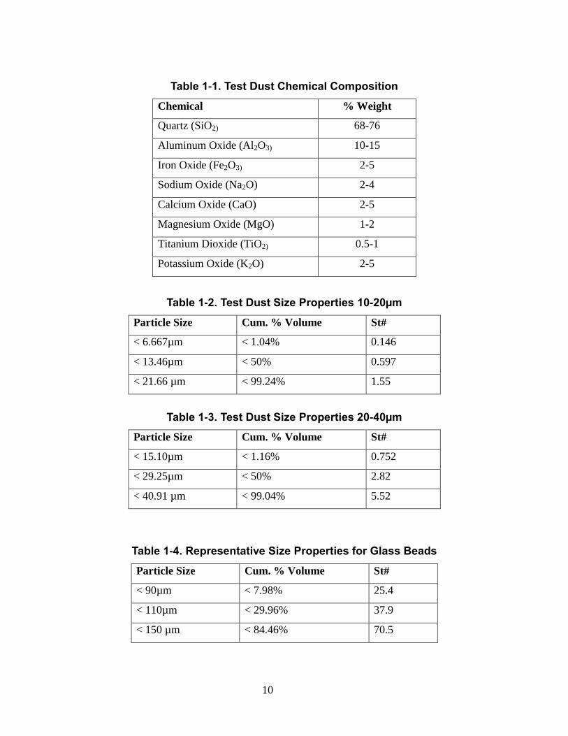
are shown in Figure 1-5. The chemical composition is presented in Table 1-1 shows the SiO2
content places the test dust in between pure quartz sand and fly ash, both of which are prone to
ingestion by a gas turbine engine. Size properties of ARD are presented in, Table 1-2, and Table
1-3 below. The size properties of the Glass Beads are presented in Table 1-4.
Figure 1-5. Size distribution of particles
10
Table 1-1. Test Dust Chemical Composition
Chemical % Weight
Quartz (SiO2) 68-76
Aluminum Oxide (Al2O3) 10-15
Iron Oxide (Fe2O3) 2-5
Sodium Oxide (Na2O) 2-4
Calcium Oxide (CaO) 2-5
Magnesium Oxide (MgO) 1-2
Titanium Dioxide (TiO2) 0.5-1
Potassium Oxide (K2O) 2-5
Table 1-2. Test Dust Size Properties 10-20µm
Particle Size Cum. % Volume St#
< 6.667µm < 1.04% 0.146
< 13.46µm < 50% 0.597
< 21.66 µm < 99.24% 1.55
Table 1-3. Test Dust Size Properties 20-40µm
Particle Size Cum. % Volume St#
< 15.10µm < 1.16% 0.752
< 29.25µm < 50% 2.82
< 40.91 µm < 99.04% 5.52
Table 1-4. Representative Size Properties for Glass Beads
Particle Size Cum. % Volume St#
< 90µm < 7.98% 25.4
< 110µm < 29.96% 37.9
< 150 µm < 84.46% 70.5

11
1.4 Data Reduction
Coefficient of restitution is defined by the particle velocities just before and just after
impact (2).
(2) 𝒆 =𝒗𝒓𝒆𝒃
𝒗𝒊𝒏
The hardware used in the VT Aerothermal Rig has a maximum repetition rate of 7.4Hz
per image pair. This does not allow for continuous tracking of particles at engine representative
speeds. This has two consequences. First is that the majority of the particle measurements are
made some distance away from the coupon. Second is that an impacting particle cannot be
uniquely identified before and after impact. The experimental approach discussed below
mitigates these consequences without the purchase of exotic or expensive imaging hardware or
software. The current setup also allows for high temperature measurements of COR, which is
the end goal of this project. The methodology discussed below is meant to establish the
technique and provide a baseline for future COR measurements.
1.4.1 Particle Tracking
The first step is to take each image pair and determine particle velocities. The particle
tracking is accomplished with an open source code developed by Grier, Crocker and Weeks and
coded for Matlab® by Blair and Dufresne.
The raw images are first filtered to increase resolution between the particles and
background. By specifying a number of parameters related to particle size and intensity, the
particles centers are then located to sub pixel accuracy in each frame of each image. The
particles are then tracked by correlating particles between frames to minimize total displacement.
A balance between particle seeding density, velocity, and time between frames must be held so
that maximum particle displacement between frames does not exceed mean particle spacing.
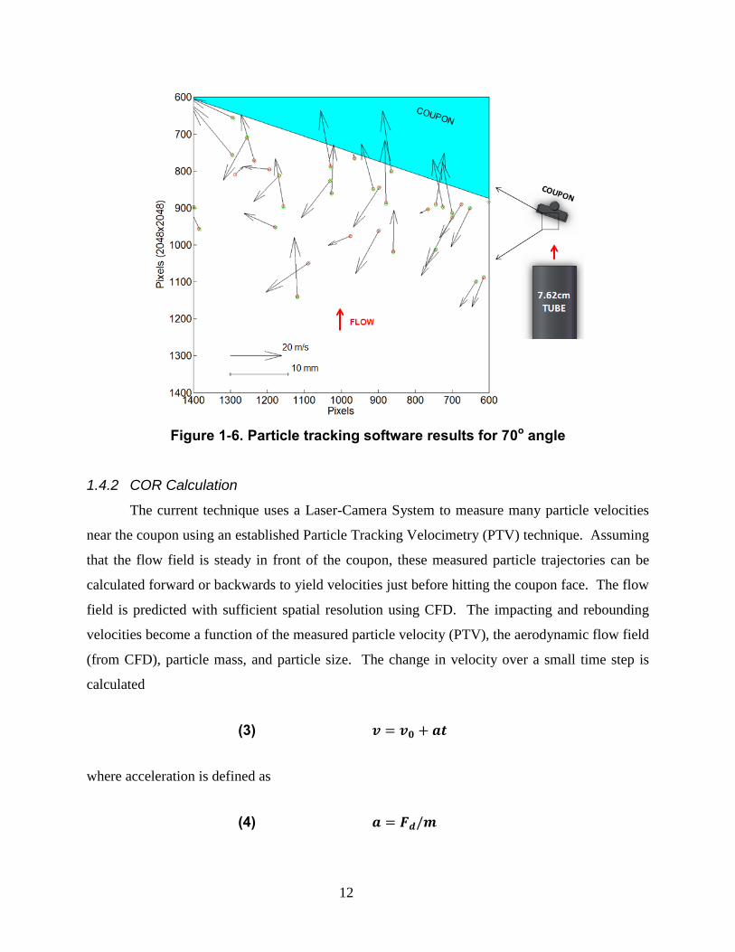
The current experiment uses image pairs in which the illuminating pulses occurs 15µs apart. A
tracked image pair is presented in Figure 1-6 with green circles representing particles in frame 1,
particles in frame 2 as red circles, and black arrows as tracked velocities between frames 1 and 2.
12
Figure 1-6. Particle tracking software results for 70o angle
1.4.2 COR Calculation
The current technique uses a Laser-Camera System to measure many particle velocities
near the coupon using an established Particle Tracking Velocimetry (PTV) technique. Assuming
that the flow field is steady in front of the coupon, these measured particle trajectories can be
calculated forward or backwards to yield velocities just before hitting the coupon face. The flow
field is predicted with sufficient spatial resolution using CFD. The impacting and rebounding
velocities become a function of the measured particle velocity (PTV), the aerodynamic flow field
(from CFD), particle mass, and particle size. The change in velocity over a small time step is
calculated
(3) 𝒗 = 𝒗𝟎 + 𝒂𝒕
where acceleration is defined as
(4) 𝒂 = 𝑭𝒅/𝒎
13
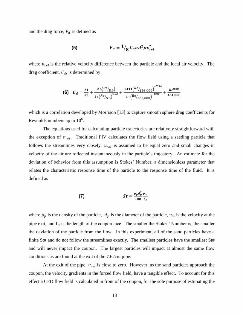
and the drag force, , is defined as
(5) 𝑭𝒅 = 𝟏𝟖⁄ 𝑪𝒅𝝅𝒅
𝟐𝝆𝒗𝒓𝒆𝒍𝟐
where is the relative velocity difference between the particle and the local air velocity. The
drag coefficient, , is determined by
(6) 𝑪𝒅 =𝟐𝟒
𝑹𝒆+
𝟐.𝟔(𝑹𝒆 𝟓.𝟎⁄ )
𝟏+(𝑹𝒆 𝟓.𝟎⁄ )𝟏.𝟓𝟐 +
𝟎.𝟒𝟏𝟏(𝑹𝒆 𝟐𝟔𝟑,𝟎𝟎𝟎⁄ )−𝟕.𝟗𝟒
𝟏+(𝑹𝒆 𝟐𝟔𝟑,𝟎𝟎𝟎⁄ )−𝟖.𝟎𝟎 +
𝑹𝒆𝟎.𝟖𝟎
𝟒𝟔𝟏,𝟎𝟎𝟎
which is a correlation developed by Morrison [13] to capture smooth sphere drag coefficients for
Reynolds numbers up to 106.
The equations used for calculating particle trajectories are relatively straightforward with
the exception of . Traditional PIV calculates the flow field using a seeding particle that
follows the streamlines very closely, is assumed to be equal zero and small changes in
velocity of the air are reflected instantaneously in the particle’s trajectory. An estimate for the
deviation of behavior from this assumption is Stokes’ Number, a dimensionless parameter that
relates the characteristic response time of the particle to the response time of the fluid. It is
defined as
(7) 𝑺𝒕 =𝝆𝒑𝒅𝒑
𝟐
𝟏𝟖𝝁
𝒗∞
𝑳𝒄
where is the density of the particle, is the diameter of the particle, is the velocity at the
pipe exit, and Lc is the length of the coupon face. The smaller the Stokes’ Number is, the smaller
the deviation of the particle from the flow. In this experiment, all of the sand particles have a
finite St# and do not follow the streamlines exactly. The smallest particles have the smallest St#
and will never impact the coupon. The largest particles will impact at almost the same flow
conditions as are found at the exit of the 7.62cm pipe.
At the exit of the pipe, is close to zero. However, as the sand particles approach the
coupon, the velocity gradients in the forced flow field, have a tangible effect. To account for this
effect a CFD flow field is calculated in front of the coupon, for the sole purpose of estimating the

14
relative velocity difference between the particle and the flow at its calculated location. This is
where the novelty of the hybrid PTV/CFD technique is witnessed, the calculation of for a
particle with a moderate Stokes #.
PTV typically captures a sparsely seeded particle through multiple images to determine a
trajectory; this is a difficult and expensive experiment at relatively high speed, engine
representative conditions. CFD can typically capture particle trajectories quite well; however,
particle impact is not accurately modeled, leading to false trajectories after an impact. By
combining the PTV measurements with CFD predictions the advantages of each technique are
maintained, while the shortcomings are negated.
Figure 1-7. Example tracked ARD 20-40µm history
The coupon face is located in the raw image to select valid impact areas at different
coupon angles. A zero point is also chosen for referencing the location of the coupon face in
both the images and the CFD. The particle measurements are then scaled, translated, and rotated
15
onto the CFD results. The measurements are then filtered into two categories, incoming and
rebounding. This categorization is a function of the current angle of trajectory compared with
the plate angle. Particles that have impacted the coupon will rebound and move away from it at
an angle different than the incoming particles. The rebounding particles are stepped backwards
to the coupon face, while the incoming particles are stepped forward until they hit the coupon
face. A set of image pairs is plotted in Figure 1-7 with the trace history of both incoming and
rebounding particle velocities.
As mentioned previously, the particles cannot be uniquely identified before and after
impact so an average incoming velocity and angle are used. The incoming velocity is a function
of impact location along the coupon face. The flow near the edges tends to turn more than the
flow in the center of the coupon and the particles impinge at steeper angles. The representative
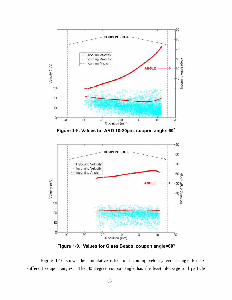
incoming data is plotted along with the raw rebounding data. An example for a given coupon
angle of 60 degree is presented in Figure 1-8 for ARD 10-20µm and in Figure 1-9 for Glass
Beads.
From these figures, it can be seen that a range of impact conditions are achieved from a
single coupon angle. The forced flowfield around the coupon also causes particles to decelerate
when approaching the impact location. For the glass beads and the ARD 20-40µm, this effect is
negligible, however, as particle size and Stokes number decrease so does the impact velocity. In
Figure 1-8, the particles impacting near the stagnation point decelerate to approximately 14 m/s
while the particles near the edge impact at approximately 19 m/s. This can have a tangible effect
on the COR results for a finite size distribution using this technique.
16
Figure 1-8. Values for ARD 10-20µm, coupon angle=60o
Figure 1-9. Values for Glass Beads, coupon angle=60o
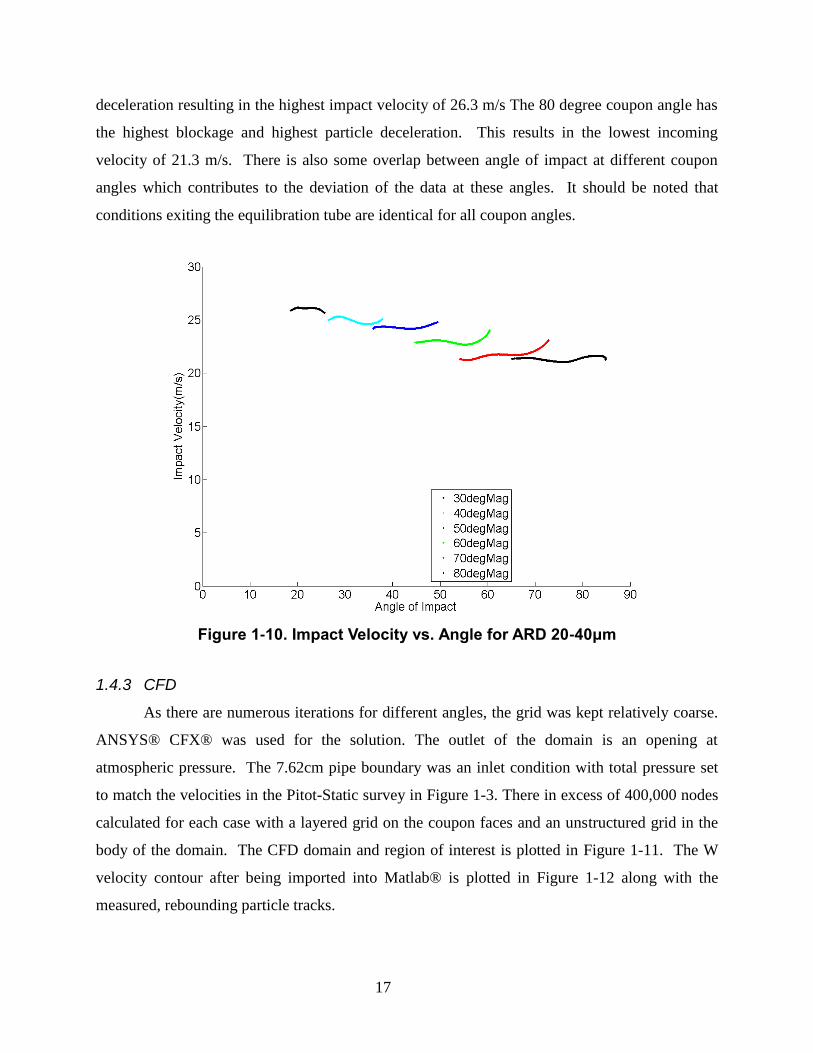
Figure 1-10 shows the cumulative effect of incoming velocity versus angle for six
different coupon angles. The 30 degree coupon angle has the least blockage and particle
17
deceleration resulting in the highest impact velocity of 26.3 m/s The 80 degree coupon angle has
the highest blockage and highest particle deceleration. This results in the lowest incoming
velocity of 21.3 m/s. There is also some overlap between angle of impact at different coupon
angles which contributes to the deviation of the data at these angles. It should be noted that
conditions exiting the equilibration tube are identical for all coupon angles.
Figure 1-10. Impact Velocity vs. Angle for ARD 20-40μm
1.4.3 CFD
As there are numerous iterations for different angles, the grid was kept relatively coarse.
ANSYS® CFX® was used for the solution. The outlet of the domain is an opening at
atmospheric pressure. The 7.62cm pipe boundary was an inlet condition with total pressure set
to match the velocities in the Pitot-Static survey in Figure 1-3. There in excess of 400,000 nodes
calculated for each case with a layered grid on the coupon faces and an unstructured grid in the
body of the domain. The CFD domain and region of interest is plotted in Figure 1-11. The W
velocity contour after being imported into Matlab® is plotted in Figure 1-12 along with the
measured, rebounding particle tracks.

18
Figure 1-11. CFD domain with W velocity Contour
Figure 1-12. W velocity CFD w/ rebounding particle tracks
19
The aerodynamic CFD is of secondary importance to the particle tracking measurements
in this experiment. Sensitivity studies were conducted to ensure undue influence was not being
exerted by incorrect velocity predictions. The aerodynamic flowfield was artificially increased
by 15% and the data re-reduced using this new flow field. Mean results were shown to decrease
by 6.8%. Measurement uncertainty was calculated at 5.4% for the inlet Pitot-static velocity
traverse used to match the CFD data to the experiment. The standard deviation in these
measurements was 2.2%. These statistics suggest that errors related to the CFD are less than
1.0% of total COR. By comparison, the average run to run repeatability of the total COR mean
values for two different data sets was 1.5%.
1.5 Results
1.5.1 Uncertainty
In the following results, raw data, mean COR, and values corresponding to one standard
deviation from the mean value are plotted. To calculate the statistical values, the data is sorted
into bins by integer value of angle of impact. In each bin, at least 100 impact events are captured
and averaged to calculate the mean. The standard deviation is calculated for each bin and plotted
accordingly.
1.5.2 Glass Beads
Glass beads were tested in this experiment to help validate the technique. They were
relatively smooth on the surface and large enough not to be significantly affected by the
flowfield downstream of the jet. Sets of data were taken at three coupon angles, 80o, 70
o, and
60o, where 90
o is normal to the flow direction. This resulted in particle impact angles from 56
o
to 83o for the beads. The average COR values for each set of data is plotted in Figure 1-13 along
with a median curve fit and upper and lower bounds.

20
Figure 1-13. Glass Bead results
The Glass bead values are in agreement with literature for glass/steel impact events.
Dunn et. al. [14], while studying microparticle adhesion, found 8.6µm mean diameter Ag-coated
glass spheres impacting stainless steel at 21m/s and 90o, to have a mean COR of 0.84. Adhesion
was not found to affect these particles at less than 15 m/s. At an 80o impact angle, the glass
beads in the current study had a mean COR of 0.81. Li et. al. [15] measured low velocity (<
1.6m/s) impact of 70µm mean diameter stainless steel spheres on a Si02 surface at different
angles. The mean COR stayed relatively constant at 0.70 for different angles above 50o.
However, microparticle adhesion did play a role at such low velocities which helps explain the
lower values of COR. Finally, [9] studied 100µm glass beads impacting polished steel at
shallow angles of impact (< 50o). A relatively constant mean COR between 0.85 and 0.8 from
impact angles of 10o to 40
o was measured. Both glass and SS are rigid, hard materials which at
low relatively low velocities should transfer their energy efficiently resulting in a high COR. At
these impact conditions, results are relatively constant between 0.79 and 0.83 with the mean
value at 0.82, which is in consistent agreement with similar experiments.
21
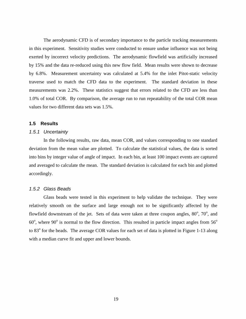
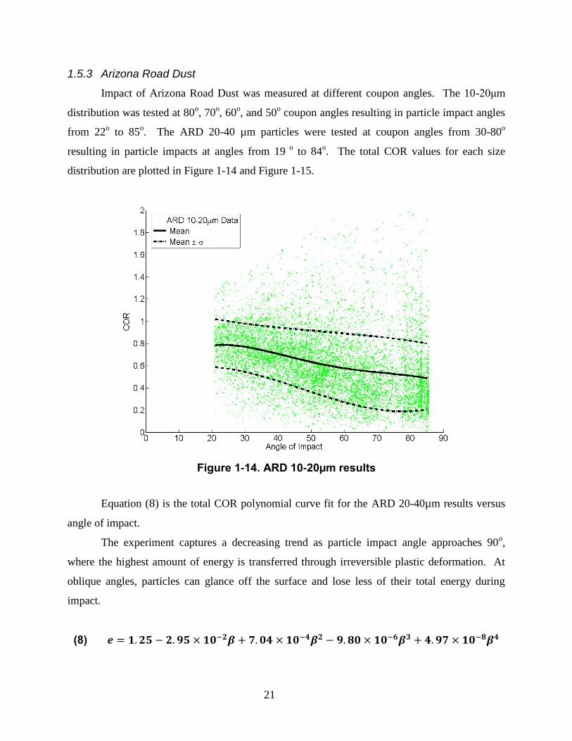
1.5.3 Arizona Road Dust
Impact of Arizona Road Dust was measured at different coupon angles. The 10-20μm
distribution was tested at 80o, 70
o, 60
o, and 50
o coupon angles resulting in particle impact angles
from 22o to 85
o. The ARD 20-40 µm particles were tested at coupon angles from 30-80
o
resulting in particle impacts at angles from 19 o
to 84o. The total COR values for each size
distribution are plotted in Figure 1-14 and Figure 1-15.
Figure 1-14. ARD 10-20µm results
Equation ( ) is the total COR polynomial curve fit for the ARD 20-40µm results versus
angle of impact.
The experiment captures a decreasing trend as particle impact angle approaches 90o,
where the highest amount of energy is transferred through irreversible plastic deformation. At
oblique angles, particles can glance off the surface and lose less of their total energy during
impact.
(8) 𝒆 = 𝟏. 𝟐𝟓 − 𝟐. 𝟗𝟓 × 𝟏𝟎 𝟐𝜷 + 𝟕. 𝟎𝟒 × 𝟏𝟎 𝟒𝜷𝟐 − 𝟗. 𝟖𝟎 × 𝟏𝟎 𝟔𝜷𝟑 + 𝟒. 𝟗𝟕 × 𝟏𝟎 𝟖𝜷𝟒
22
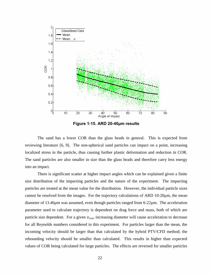
Figure 1-15. ARD 20-40µm results
The sand has a lower COR than the glass beads in general. This is expected from
reviewing literature [6, 9]. The non-spherical sand particles can impact on a point, increasing
localized stress in the particle, thus causing further plastic deformation and reduction in COR.
The sand particles are also smaller in size than the glass beads and therefore carry less energy
into an impact.
There is significant scatter at higher impact angles which can be explained given a finite
size distribution of the impacting particles and the nature of the experiment. The impacting
particles are treated at the mean value for the distribution. However, the individual particle sizes
cannot be resolved from the images. For the trajectory calculations of ARD 10-20µm, the mean
diameter of 13.46µm was assumed, even though particles ranged from 6-22µm. The acceleration
parameter used to calculate trajectory is dependent on drag force and mass, both of which are
particle size dependent. For a given , increasing diameter will cause acceleration to decrease
for all Reynolds numbers considered in this experiment. For particles larger than the mean, the
incoming velocity should be larger than that calculated by the hybrid PTV/CFD method; the
rebounding velocity should be smaller than calculated. This results in higher than expected
values of COR being calculated for large particles. The effects are reversed for smaller particles

23
with a high enough St# to impact the coupon, these smaller particles will contribute to lower than
expected COR values. The COR values above one in Figure 1-14 and Figure 1-15 are not
physically possible. They are a result of statistical processing in this technique but are included
so an accurate mean can be reported for this ARD distribution.
Even with the size distribution accounted for, scatter would still be expected, COR
experiments are statistical in nature [6, 7]. In even the most controlled experiments non-
spherical particles and minute surface roughness will cause variation in the measured data due to
the shadow effect documented in [9]. Other researchers have also documented the effects of
adhesion in microparticle impacts at low velocity which is not exhibited at larger particle sizes at
the same speeds [10].
Figure 1-16. Comparison with Literature COR vs Angle
Figure 1-16 compares mean values with [6, 7], a similar trend is exhibited for fly ash and
sand impacts. A few caveats must be noted, first, that the sand particles in the comparison
experiment are 150µm while the fly ash is 15µm. The fly ash is included for a size comparison
even though it possesses a different chemical composition. The impact speeds are greater than
91m/s so both of these particles impact with greater energy than the ARD particles in this study.
24
Also different grades of steel are used as impact surfaces. With that said, these are the closest
experimental comparisons available in open literature for microparticle sand and ash at different
angles of impact. The comparison is quite good with the differences in impact energy
accounting for lower values of COR.
1.5.4 Normal & Tangential COR
As the ultimate goal of this work is to measure engine realistic impact conditions and
how they relate to erosion and deposition, it is also important to look at the role of tangential and
normal components of COR for oblique impacts. These components can be extracted from the
data by looking at the rebound trajectory as predicted at the coupon surface and comparing to the
representative incoming values for angle and velocity magnitude. Figure 1-17 shows the mean
and deviation for tangential COR versus angle of impact. Equation (9) gives the polynomial
relationship for the mean value of tangential COR as a function of angle of impact.
Figure 1-18 is also included to show the relationship between the representative
tangential impact velocity and the angle of impact. Due to the limitations of the facility,
independent variation of the tangential and normal components of velocity is not currently
possible. This resulted in the tangential and normal components of impact velocity, varying with
coupon angle. This should not affect the comparison with literature since there is no mention of
incoming conditions other than the bulk velocity. From these results, the large variation (and
negative values) seen in Figure 1-17 at high impact angles can be explained by the low tangential
component velocity at high angles of impact. Any noise introduced by normal particle variation
during rebound will be magnified by the small denominator in Equation (2).
(9) 𝒆𝒕 = 𝟏. 𝟗𝟏 − 𝟎. 𝟏𝟏𝟓𝜷 + 𝟒. 𝟐𝟎 × 𝟏𝟎 𝟑𝜷𝟐 − 𝟔. 𝟒𝟔 × 𝟏𝟎 𝟓𝜷𝟑 + 𝟑. 𝟓𝟓 × 𝟏𝟎 𝟕𝜷𝟒

25
Figure 1-17. Tangential COR vs Angle ARD 20-40μm
Figure 1-18. Tangential Velocity vs Angle for ARD 20-40μm
26
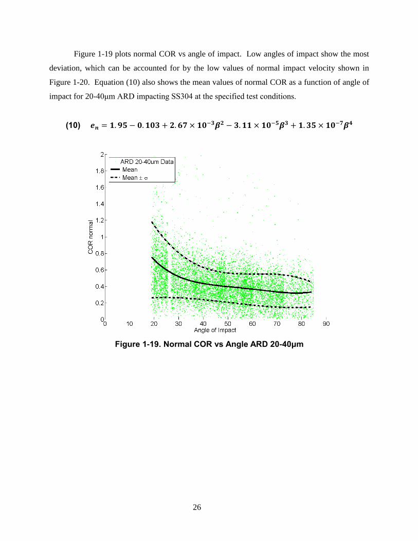
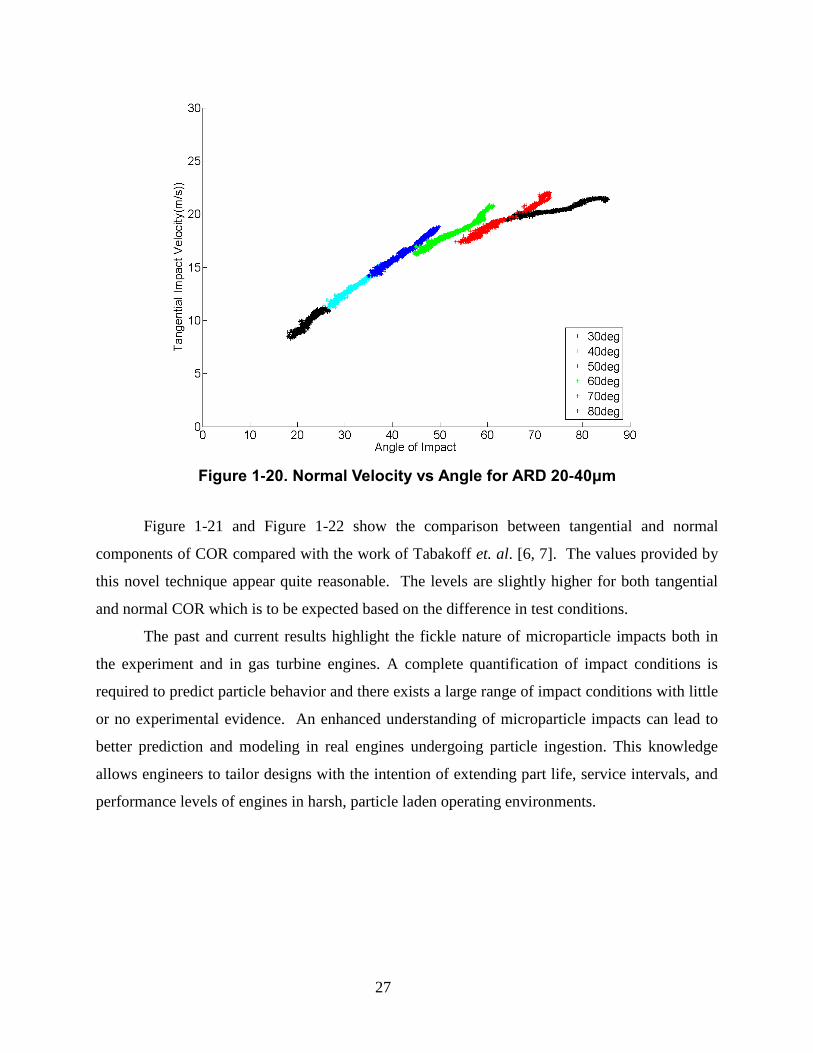
Figure 1-19 plots normal COR vs angle of impact. Low angles of impact show the most
deviation, which can be accounted for by the low values of normal impact velocity shown in
Figure 1-20. Equation (10) also shows the mean values of normal COR as a function of angle of
impact for 20-40μm ARD impacting SS304 at the specified test conditions.
(10) 𝒆𝒏 = 𝟏. 𝟗𝟓 − 𝟎. 𝟏𝟎𝟑 + 𝟐. 𝟔𝟕 × 𝟏𝟎 𝟑𝜷𝟐 − 𝟑. 𝟏𝟏 × 𝟏𝟎 𝟓𝜷𝟑 + 𝟏. 𝟑𝟓 × 𝟏𝟎 𝟕𝜷𝟒
Figure 1-19. Normal COR vs Angle ARD 20-40μm
27
Figure 1-20. Normal Velocity vs Angle for ARD 20-40μm
Figure 1-21 and Figure 1-22 show the comparison between tangential and normal
components of COR compared with the work of Tabakoff et. al. [6, 7]. The values provided by
this novel technique appear quite reasonable. The levels are slightly higher for both tangential
and normal COR which is to be expected based on the difference in test conditions.
The past and current results highlight the fickle nature of microparticle impacts both in
the experiment and in gas turbine engines. A complete quantification of impact conditions is
required to predict particle behavior and there exists a large range of impact conditions with little
or no experimental evidence. An enhanced understanding of microparticle impacts can lead to
better prediction and modeling in real engines undergoing particle ingestion. This knowledge
allows engineers to tailor designs with the intention of extending part life, service intervals, and
performance levels of engines in harsh, particle laden operating environments.

28
Figure 1-21. Tangential COR vs Angle ARD 20-40μm
Figure 1-22. Normal COR vs Angle ARD 20-40μm

29
1.6 Conclusions
A new technique was presented to measure Coefficient of Restitution for Microparticle
Impacts. Data from a 27m/s free jet was presented at different angles for microparticle glass
beads and sand, impacting 304 Stainless Steel. The empirical data presented here is intended to
provide an estimate of both the mean and variance expected from an impact of these specific
materials at a given angle and velocity. The actual behavior cannot be computationally
determined accurately without investing significant resources. The results are in qualitative and
quantitative agreement with past experiments for microparticles at similar, but not identical,
sizes, angles, and velocities. This technique captures a large quantity of particle impacts over a
wider range of impact angles than previously utilized techniques. The technique can also be
applied to a high temperature environment for measuring engine realistic (high temperature /
velocity) impacts. The resulting data is of acceptable quality and can be obtained with
economical, readily-available hardware and software. Most importantly, the current dataset
completes the understanding of COR behavior for sand particles under 40μm when compared to
available literature that is limited to particle sizes above 100μm. This allows for accurate
modeling of particle transport and identification of areas susceptible to particle ingestion effects.
1.7 Acknowledgments
This paper was published in the conference proceedings for the ASME IGTI Turbo Expo
2012, the work was presented in Copenhagen, Denmark on June 15, 2012. The co-authors on
this paper are J.M. Delimont, W.F. Ng, S.V. Ekkad from Virinia Tech, Blacksburg, VA, USA
and V.P. Rajendran from Rolls-Royce, Indianapolis, IN, USA. Journal publication is currently
being sought.
The work detailed here would not be possible without the support and direction of Rolls-
Royce, especially N. Wagers, H. Kwen, M. Creason, and B. Barker. The authors would also like
to thank D.K. Tafti and S. Singh from Virginia Tech for their thoughtful discussion, analysis and
advice.
1.8 References
[1] Hertz, H., 1896, "Miscellaneous Papers by H. Hertz," MacMillan, London, pp. 142-162.
[2] Goldsmith, W., 2002, Impact : the theory and physical behaviour of colliding solids, Dover
Publications, Mineola, N.Y.
[3] Johnson, K. L., 1985, Contact Mechanics, Cambridge University Press, Cambridge, UK.
30
[4] Tabakoff, W., Grant, G., and Ball, R., 1974, "An Experimental Investigation of Certain
Aerodynamic Effects on Erosion," AIAA-74-639.
[5] Wakeman, T., and Tabakoff, W., 1979, "Erosion Behavior in a Simulated Jet Engine
Environment," J. Aircraft, 16(12), pp. 828-833.
[6] Tabakoff, W., 1991, "Measurements of Particles Rebound Characteristics on Materials Used
in Gas Turbines," J. of Propulsion and Power, 7(5), pp. 805-813.
[7] Tabakoff. W, H., A., and Murugan, D.M, 1996, "Effect of Target Materials on the Particle
Restitution Characteristics for Turbomachinery Application," J. of Propulsion and Power, 12(2),
pp. 260-266.
[8] Eroglu, H., and Tabakoff, W., 1991, "3-D LDV Measurements of Particle Rebound
Characteristics," AIAA-91-0011.
[9] Sommerfeld, M., and Huber, N., 1999, "Experimental analysis and modelling of particle-wall
collisions," International Journal of Multiphase Flow, 25, pp. 1457-1489.
[10] Wall, S., John, W., Wang H.C., and Goren, S. L., 1990, "Measurements of Kinetic Energy
Loss for Particles Impacting Surfaces," Aerosol Science and Technology, 12, pp. 926-946.
[11] Hylton, L., Nirmalan, V., Sultanian, B., Kaufman, R., 1988, "The Effects of Leading Edge
and Downstream Film Cooling on Turbine Vane Heat Transfer," NASA Contractor Report
182133.
[12] Nealy, D., Mihelc, M., Hylton, L., Gladden, H., 1984, "Measurements of Heat Transfer
Distribution Over the Surfaces of Highly Loaded Turbine Nozzle Guide Vanes," Journal of
Engineering for Gas Turbines and Power, 106, pp. 149-158.
[13] Morrison, F. A., "Data Correlation for Drag Coefficient for Sphere," Department of
Chemical Engineering, Michigan Technological University, Houghton, MI.
[14] Dunn, P. F., Brach, R. M., and Caylor, M. J., 1995, "Experiments on the Low-Velocity
Impact of Microspheres with Planar Surfaces," Aerosol Science and Technology, 23(1), pp. 80-
95.
[15] Li, X., Dunn, P.F., and Brach, R.M., 2000, "Experimental and Numerical Studies of
Microsphere Oblique Impact with Planar Surfaces," Aerosol Science and Technology, 31(5), pp.
583-594.
31
2 Paper #2: Study of Microparticle Rebound Characteristics Under High
Temperature Conditions
2.1 Abstract
Large amounts of tiny microparticles are ingested into gas turbines over their operating
life, resulting in unexpected wear and tear. Knowledge of such microparticle behavior at gas
turbine operating temperatures is limited in published literature. In this study, Arizona Test
Dust is injected into a hot flow field at temperatures of 533oK, 866
oK, and 1073
oK to measure
the effects of high temperature on particle rebound from a polished 304 Stainless Steel coupon.
The results are compared with baseline (27m/s) measurements at ambient (300oK) temperature
made in the Virginia Tech Aerothermal Rig, as well as previously published literature. Mean
Coefficient of Restitution (COR) was shown to decrease with the increased temperature/velocity
conditions in the VT Aerothermal Rig. The effects of increasing temperature and velocity led to
a 12% average reduction in COR at 533oK (47m/s), 15% average reduction in COR at 866
oK
(77m/s), and 16% average reduction in COR at 1073oK (102m/s) compared with ambient results.
From these results it is shown that a power law relationship may not conclusively fit the COR vs
temperature/velocity trend at oblique angles of impact. The decrease in COR appeared to be
almost entirely a result of increased velocity that resulted from heating the flow. Trends show
that temperature plays a minor role in energy transfer between particle and impact surface
below a critical temperature around 1300°K.
2.2 Introduction
As global transportation and energy needs continue to expand, gas turbine engines are
increasingly called upon to provide mechanical power. Many of these new or expanding markets
require engines to operate in harsh, particle laden environments. These particles can cause
performance deterioration through erosion and deposition of turbine parts.
A number of studies have looked at these mechanisms but there is a lack of fundamental
understanding of particle trajectory after impact at engine representative conditions. An
understanding of erosion rates has been established through experiments but the results and data
almost always focus on the surface and not the particle. Erosive particles will continue on
through the engine after the initial impact and may cause subsequent damage to other areas
32
downstream. The engine conditions that cause deposition are being investigated by a number of
researchers but many upstream or secondary flows in the engine do not meet the temperature or
velocity requirements to initiate deposition. However, these particles may be ejected through
film cooling holes or combustion liners, which meet conditions for deposition, after several
impacts upstream. The accurate trajectory modeling of these particles after impact can lead to a
better understanding of the particular regions most susceptible to the effects of particle ingestion.
In many modeling scenarios the effects of impact are modeled using Coefficient of
Restitution (COR). COR is defined
(11) 𝒆 =𝒗𝒓𝒆𝒃
𝒗𝒊𝒏
where is the incoming particle velocity, and is the velocity after impact. COR depends
on a number of parameters such as material properties, velocity, particle size, impact angle,
particle spin, particle sphericity, surface roughness, and temperature. The effects of these impact
parameters have been well documented by researchers studying a variety of topics. Goldsmith
[1] provided a wealth of knowledge on classical impacts investigated during the 20th
century. In
this reference, COR is shown to decrease with increasing velocity, increasing size, and
decreasing hardness. Armstrong et. al. [2] documented that particle spin could result in curved
trajectories after impact due to Magnus forces. Sommerfeld and Huber [3] documented the
effects of surface roughness and sphericity. Their study showed rougher surfaces or less
spherical particles tend to have lower COR and a wider scatter due to strong local deformations.
The effects of temperature have been largely ignored when considering COR.
There exist a few studies that can be loosely applied to the physics of engine realistic
impacts at high temperature. Mok and Duffy [4] looked at 1” steel and 2017 aluminum balls
impacting lead or 6061-T6 aluminum plates at velocities of 0-5m/s and temperatures from 294-
755oK to measure the dynamic yield stress. The impacts were shown to be elasto-plastic based
on non-dimensional parameters fit to the experimental measurements of indentation diameter and
time of contact. The ratio of yield stress and Young’s modulus was shown to vary little with
temperature. COR results versus velocity were presented at 90o impact angle. The effect of
temperature on the steel ball, lead specimen impact event was negligible, likely due to the
relative softness of lead. The effect of temperature on the steel ball, aluminum alloy specimen

33
impact event was notable. COR was decreased ~0.08 at different impact velocities by increasing
temperature from 294oK to 755
oK
Brenner et al. [5] impinged three types of iron spheres on iron plates in a hydrogen
atmosphere to look at the various effects related to temperature, surface coating, roughness,
sphere size, and oxygen levels. Impact area, sticking probability and COR results were
presented at 90o impact angles. COR results were shown for 973 and 1073
oK, type II spheres
(melted drops of 120μm thick wire) impacting an Al2O3 coated iron plate at velocities up to
3m/s. COR was reduced by ~0.03 between these two temperatures. COR was shown to be
proportional to ⁄ at 90
o impact for one of the 1073
oK test cases.
However, the conditions of these two studies cannot be considered engine representative
due to the materials and particles sizes tested. Erosive behavior of aerospace materials has been
associated with COR through a number of works by Tabakoff et. al. [6-9]. In these works, COR
is shown to be statistical in nature. These works also show that erosion is primarily a function of
tangential COR for large quartz particles. At shallow impact angles erosion is the highest, even
though bounce-back is quite efficient at these angles, resulting in a high total COR. This was
evidenced previously in the models of Finnie [10] for ductile erosion. However, only one
Tabakoff study looks at particles small enough to be considered engine representative, where
15μm fly ash particles impact aerospace materials at ambient temperature. Erosion was not
presented in this work. Wakeman and Tabakoff [11] looked at erosive behavior at temperatures
up to 978oK, impact velocities up to 274m/s, and different impact angles for 150-180μm quartz
sand particles. A power law relationship was shown to fit the erosive data for increasing velocity
quite well, though the coefficients varied with changing impact angle and material. However,
the COR was not presented for these test cases.
Still, COR has not been transparently presented for high temperature, engine
representative particles at different angles and velocities. It is clear that more study is needed on
the topic to accurately represent particle transport and energy transfer mechanisms in
computational models. This work is intended to help fill in the gap between erosion and
deposition experiments in literature. Erosive experiments neglect the particle after impact and
deposition experiments only quantify a sticking probability associated with high temperature
impact. With the current hardware at Virginia Tech and the measurement technique established

34
by the authors, the problem of high temperature microparticle impact in turbomachinery
environments is investigated in the following work.
2.2.1 Nomenclature
Coefficient of Restitution (COR)
E Elastic (Young’s) Modulus
mass
Stokes Number
Velocity
Y Yield Strength (0.2% Offset)
β angle of impact
σ standard deviation
Subscript
in incoming
n normal
reb rebound
t tangential
2.3 Experimental Setup and Instrumentation
2.3.1 Aerothermal Rig
Virginia Tech Aerothermal Rig was donated to Virginia Tech by Rolls-Royce in
September 2010. This rig was used in previous heat transfer studies conducted at their facility in
Indianapolis, IN by Hylton et al. [12] and Nealy et al. [13]. The operational specifications for
this rig when installed in Indianapolis were reported as 2.2kg/s at a maximum of 16atm and
2033K by Rolls-Royce. For the present study the Aerothermal Rig has been reconfigured to
allow for sand injection into the flow as seen in Figure 2-1. The rig was used by Reagle et. al.
[14] in this configuration to measure the baseline results at ambient temperature.
At Virginia Tech, the pressure and temperature capabilities for this rig are being brought
up in steps as the rig is fully recomissioned. The first step in this gradual process is igniting the

35
burner, which is water cooled, to temperatures within the safe operating limits of the uncooled
equilibrate and test sections.
Figure 2-1. VT Aerothermal Rig configured for sand testing
A compressor supplies air to the rig at a constant rate of 0.15kg/s. The flow is regulated
upstream with a 10.2cm globe valve. The air then passes through a sudden expansion burner
capable of heating the flow. The burner has a fuel ring capable of supplying 12 nozzles used to
heat the flow. In the current study, temperature levels of 533oK, the minimum stable operating
limit of the burner, and up to 1073oK, the current safe operating limit for the uncooled materials,
are tested. The methane exiting these nozzles is initially ignited using a hydrogen/air pilot light.
Due to the fixed mass flow rate being used in this test configuration the velocity and temperature
are not controlled independently. This means that as temperature increases the velocity also
increases in a proportional manner. The VT Aerothermal Rig is typically heated for one hour
prior to the first test. Once thermocouples on the coupon, in the contraction, and in the exhaust
all reach steady values, particles are injected and measurements are obtained.
At the exit downstream of the burner, the cross-section of the flow is reduced in diameter
from 30.5cm to 7.62cm. During the contraction section, the test particles are injected into the
mainstream flow. The particles are entrained in a compressed air flow that is supplied from the
main compressor upstream of the burner. The particles then enter a 1.82m long, 7.62cm
36
diameter equilibration tube which enables particles of various sizes to accelerate to the same
speed (and temperature) as the rest of the flow. The flow exits the equilibration tube as a free jet
into the test section and impinges on the test surface.
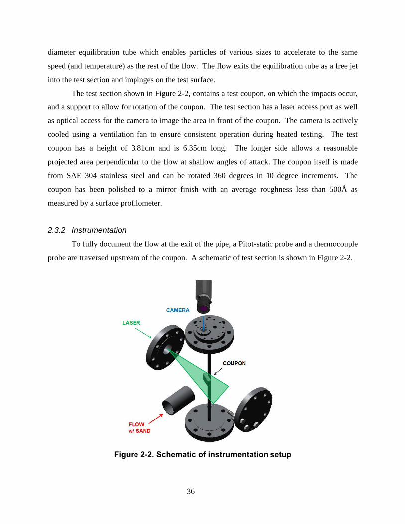
The test section shown in Figure 2-2, contains a test coupon, on which the impacts occur,
and a support to allow for rotation of the coupon. The test section has a laser access port as well
as optical access for the camera to image the area in front of the coupon. The camera is actively
cooled using a ventilation fan to ensure consistent operation during heated testing. The test
coupon has a height of 3.81cm and is 6.35cm long. The longer side allows a reasonable
projected area perpendicular to the flow at shallow angles of attack. The coupon itself is made
from SAE 304 stainless steel and can be rotated 360 degrees in 10 degree increments. The
coupon has been polished to a mirror finish with an average roughness less than 500Å as
measured by a surface profilometer.
2.3.2 Instrumentation
To fully document the flow at the exit of the pipe, a Pitot-static probe and a thermocouple
probe are traversed upstream of the coupon. A schematic of test section is shown in Figure 2-2.
Figure 2-2. Schematic of instrumentation setup

37
Figure 2-3. Traverse 8.13cm Upstream of Coupon at 533oK
Figure 2-4. Temperature Ratio 1.78cm Upstream of Coupon

38
The Pitot-static probe survey, seen in Figure 2-3, was taken at a distance of 8.13cm
upstream from the coupon face to quantify the fully developed velocity profile. The Reynolds
number at the survey location is 94,000 for the 533oK case, 69,000 for the 866
oK case, and
60,000 for the 1073oK case based on the diameter of the pipe.
The thermocouple survey shown in Figure 2-4 plots the value of the thermocouple ratio
between the probe measurement location, and a fixed thermocouple downstream of the test
section. The survey shows a flat temperature profile upstream of the coupon.
The laser for illuminating the particles is a twin head Litron Nd:YAG laser that emits
approximately 135mJ at 532nm wavelength. The laser is capable of emitting two pulses of light
within a few microseconds. The laser light is projected in a plane at the center of the test coupon
as shown in Figure 2-2. A Dantec Dynamics® FlowSense camera equipped with a Zeiss®
Makro-Planar 2/50 lens is used to capture the particle images at 2048x2048 resolution. Both the
laser and the camera are synced by a timer box ensuring illumination and imaging occur
concurrently. The system can take image pairs with a 5μs, however, the maximum sampling
frequency for image pairs is 7.4Hz.
2.3.3 Test Conditions and Material Properties
The sand particles used were Arizona Test Dust. Intermediate grades of nominal 20-40
µm were tested in this experiment. Arizona road dust (ARD) has been widely used as a standard
test dust for filtration, automotive and heavy equipment testing. It is also an excellent choice for
studying sand ingestion in jet engines as it has very similar properties to sands found throughout
the world and is readily available. The mean size by volume is 29.25μm. More detailed
information on the test dust size can be found in [14]. The chemical composition and melting
point of the various constituents is presented in Table 2-1. Based on SiO2 composition, these
particles fall somewhere between pure silica sand and fly ash. Tests conducted by Walsh et
al.[15] in a temperature controlled kiln show that a similar mixture of sand began to have visible
temperature effects at 1203oK with complete melting occurring by 1363
oK.
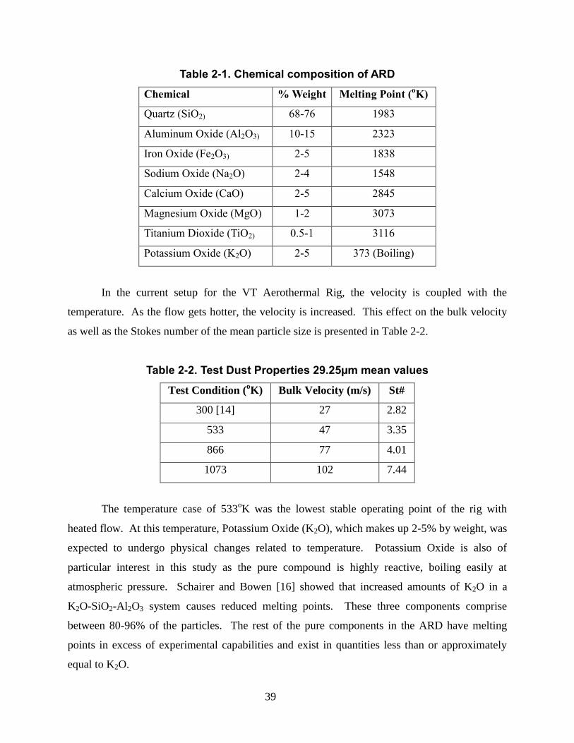
39
Table 2-1. Chemical composition of ARD
Chemical % Weight Melting Point (oK)
Quartz (SiO2) 68-76 1983
Aluminum Oxide (Al2O3) 10-15 2323
Iron Oxide (Fe2O3) 2-5 1838
Sodium Oxide (Na2O) 2-4 1548
Calcium Oxide (CaO) 2-5 2845
Magnesium Oxide (MgO) 1-2 3073
Titanium Dioxide (TiO2) 0.5-1 3116
Potassium Oxide (K2O) 2-5 373 (Boiling)
In the current setup for the VT Aerothermal Rig, the velocity is coupled with the
temperature. As the flow gets hotter, the velocity is increased. This effect on the bulk velocity
as well as the Stokes number of the mean particle size is presented in Table 2-2.
Table 2-2. Test Dust Properties 29.25µm mean values
Test Condition (oK) Bulk Velocity (m/s) St#
300 [14] 27 2.82
533 47 3.35
866 77 4.01
1073 102 7.44
The temperature case of 533oK was the lowest stable operating point of the rig with
heated flow. At this temperature, Potassium Oxide (K2O), which makes up 2-5% by weight, was
expected to undergo physical changes related to temperature. Potassium Oxide is also of
particular interest in this study as the pure compound is highly reactive, boiling easily at
atmospheric pressure. Schairer and Bowen [16] showed that increased amounts of K2O in a
K2O-SiO2-Al2O3 system causes reduced melting points. These three components comprise
between 80-96% of the particles. The rest of the pure components in the ARD have melting
points in excess of experimental capabilities and exist in quantities less than or approximately
equal to K2O.
40
The temperature case of 866oK was chosen because SiO2 undergoes a crystal
transformation from α-quartz to β-quartz at a temperature of 846oK and normal pressure. This
change occurs quite suddenly and comes with a change in bond angle and an expansion from
2.65g/cm3
to 2.53g/cm3.
The 1073oK test case was chosen as an acceptable operating limit for the stainless steel
test section components which were not actively cooled. It was hypothesized that this high of
temperature would cause a relative change in material properties between the particle and the
coupon leading to a significant reduction in COR. This was within 130oK of the critical
temperature for the sand as shown in [15].
2.4 Data Reduction
Coefficient of restitution is defined by the particle velocities just before and just after
impact. The hardware used in the VT Aerothermal Rig has a maximum repetition rate of 7.4Hz
per image pair. This does not allow for continuous tracking of particles at engine representative
speeds. This has two consequences. First is that the majority of the particle measurements are
made some distance away from the coupon. Second is that an impacting particle cannot be
uniquely identified before and after impact. The experimental approach discussed in [14]
mitigates these consequences without the purchase of exotic or expensive imaging hardware or
software. A brief summary is presented below.
The first step is to take each image pair and determine particle velocities. The raw
images are filtered to increase contrast between the particles and background. The particles are
then tracked by correlating particle locations between frames to minimize total displacement.
The particles are classified as incoming or rebounding based on their trajectory angle with
respect to the coupon angle. Assuming that the flow field is steady in front of the coupon, these
measured particle trajectories can be calculated forward or backwards in time using a finite
difference method to yield velocities just before hitting the coupon face. The impacting and
rebounding velocities become a function of the measured particle velocity, the relative velocity
of the particle, particle mass, and particle size.
The equations used for calculating particle trajectories are relatively straightforward with
the exception of , the relative velocity between the flow and the particle. At the exit of the
pipe, is close to zero. However, as the sand particles approach the plate, the velocity
41
gradient in the forced flow field has a tangible effect on the particle trajectory. To account for
this effect, a CFD flow field is calculated in front of the coupon for the sole purpose of
estimating the relative velocity difference between the particle and the flow at its current location
in the finite difference calculation. The particle measurements are then mapped onto the CFD
flowfield and tracked to the coupon face. The incoming velocity is then calculated as a function
of impact location along the coupon face. The rebounding particle data is then combined with
incoming particle data to calculate COR for each rebounding particle.
This results in a range of particle impact angles for a single coupon angle. At high
temperatures, the cost of testing for extended periods can be quite high, especially as more mass
flow is added and the rig is brought up to full capability. The current technique allows for
collection of thousands of impact events in a relatively short data taking window. This also
helps to eliminate the effects of erosion on the coupon, which can significantly affect results.
Surface roughness measurements following a set of heated runs showed average roughness to
have increased, but still remained less than 1000Å.
2.5 Results
The results published here document the effects of temperature/velocity on microparticle
sand impacting stainless steel 304 at different angles. The results and polynomials can be
incorporated into user defined functions for commercial or proprietary CFD codes. This allows
for accurate modeling of particle transport with realistic impact physics. An example application
for this data would be particles in an internal cooling channel of a cooled airfoil in a gas turbine
engine. The cooling air is bled from the compressor which may ingest large quantities of
particulate matter while operating in a harsh environment.
2.5.1 Uncertainty
In the following results, only the mean COR values are plotted for clarity. Raw data and
standard deviation with respect to impact angle has been presented in previous works [14] for
ambient data and will be omitted for clarity. The average deviation for COR across all test cases
is σ = 0.17. The values for normal and tangential components varied widely with angle. At
angles up to 48o, σt was less than 0.3 for all cases while at angles above 74
o resulted in σt values
above 1 for all cases. For normal COR, σn decreased from a maximum of 0.43 at 19o angles to

42
less than 0.2 at angles greater than 40o for all compared cases. Table 2-3 shows representative
values of deviation for COR, tangential COR, and normal COR.
Table 2-3. Average Deviation from Mean Values
Angle of Impact σ σt σn
25 0.14 0.25 0.26
35 0.15 0.27 0.21
45 0.17 0.24 0.17
55 0.18 0.31 0.17
65 0.19 0.56 0.18
75 0.18 0.95 0.16
2.5.2 Total Coefficient of Restitution
Arizona Road Dust impacting a polished stainless steel 304 coupon was measured at
coupon angles from 30-80o at four temperatures/velocities. Figure 2-5 shows the total COR
results for all four temperature/velocity conditions vs angle of impact. COR vs angle of impact
was shown to decrease at all angles as temperature/velocity increased. The raw data has been fit
to a polynomial in equations (12), (13), and (14) and present the COR as a function of impact
angle for the three heated test cases. The average decrease in COR for the increased temperature
and velocity conditions was 12% for the 533oK (47m/s), 15% for the 866
oK (77m/s) case, and
16% for the 1073oK (102m/s) case over the baseline COR results.
(12) 𝒆𝒗,𝟓𝟑𝟑𝑲 = 𝟏. 𝟎𝟔 − 𝟐. 𝟐𝟖 × 𝟏𝟎 𝟐𝜷 + 𝟓. 𝟑𝟕 × 𝟏𝟎 𝟒𝜷𝟐 − 𝟖. 𝟎𝟐 × 𝟏𝟎 𝟔𝜷𝟑 +
𝟒. 𝟒𝟎 × 𝟏𝟎 𝟖𝜷𝟒
(13) 𝒆𝒗,𝟖𝟔𝟔𝑲 = 𝟏. 𝟎𝟑 − 𝟐. 𝟎𝟗 × 𝟏𝟎 𝟐𝜷 + 𝟒. 𝟒𝟑 × 𝟏𝟎 𝟒𝜷𝟐 − 𝟔. 𝟑𝟐 × 𝟏𝟎 𝟔𝜷𝟑 +
𝟑. 𝟑𝟗 × 𝟏𝟎 𝟖𝜷𝟒
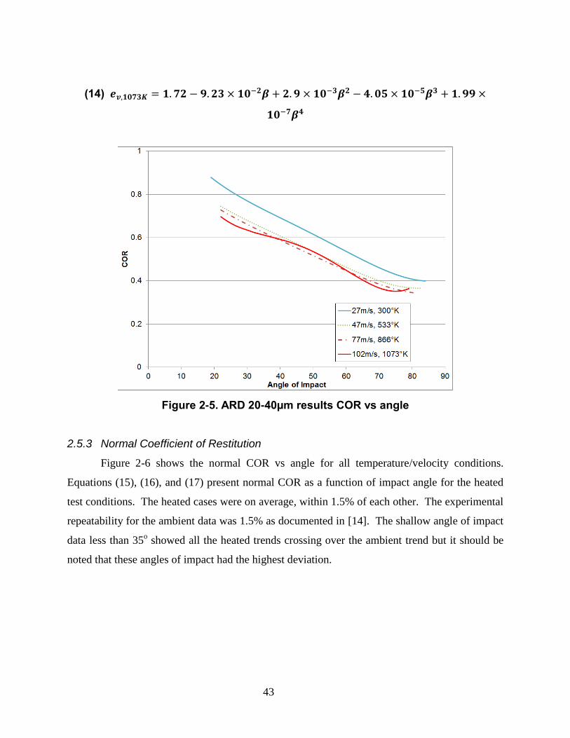
43
(14) 𝒆𝒗,𝟏𝟎𝟕𝟑𝑲 = 𝟏. 𝟕𝟐 − 𝟗. 𝟐𝟑 × 𝟏𝟎 𝟐𝜷 + 𝟐. 𝟗 × 𝟏𝟎 𝟑𝜷𝟐 − 𝟒. 𝟎𝟓 × 𝟏𝟎 𝟓𝜷𝟑 + 𝟏. 𝟗𝟗 ×
𝟏𝟎 𝟕𝜷𝟒
Figure 2-5. ARD 20-40µm results COR vs angle
2.5.3 Normal Coefficient of Restitution
Figure 2-6 shows the normal COR vs angle for all temperature/velocity conditions.
Equations (15), (16), and (17) present normal COR as a function of impact angle for the heated
test conditions. The heated cases were on average, within 1.5% of each other. The experimental
repeatability for the ambient data was 1.5% as documented in [14]. The shallow angle of impact
data less than 35o showed all the heated trends crossing over the ambient trend but it should be
noted that these angles of impact had the highest deviation.
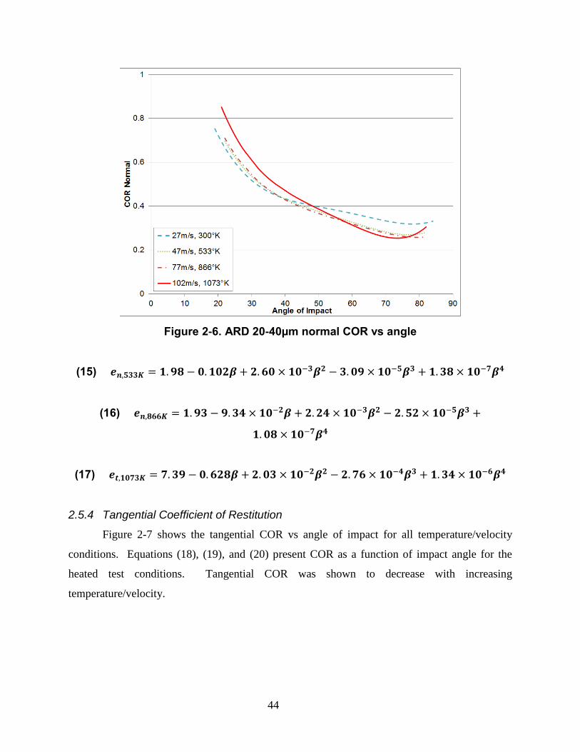
44
Figure 2-6. ARD 20-40µm normal COR vs angle
(15) 𝒆𝒏,𝟓𝟑𝟑𝑲 = 𝟏. 𝟗𝟖 − 𝟎. 𝟏𝟎𝟐𝜷 + 𝟐. 𝟔𝟎 × 𝟏𝟎 𝟑𝜷𝟐 − 𝟑. 𝟎𝟗 × 𝟏𝟎 𝟓𝜷𝟑 + 𝟏. 𝟑𝟖 × 𝟏𝟎 𝟕𝜷𝟒
(16) 𝒆𝒏,𝟖𝟔𝟔𝑲 = 𝟏. 𝟗𝟑 − 𝟗. 𝟑𝟒 × 𝟏𝟎 𝟐𝜷 + 𝟐. 𝟐𝟒 × 𝟏𝟎 𝟑𝜷𝟐 − 𝟐. 𝟓𝟐 × 𝟏𝟎 𝟓𝜷𝟑 +
𝟏. 𝟎𝟖 × 𝟏𝟎 𝟕𝜷𝟒
(17) 𝒆𝒕,𝟏𝟎𝟕𝟑𝑲 = 𝟕. 𝟑𝟗 − 𝟎. 𝟔𝟐𝟖𝜷 + 𝟐. 𝟎𝟑 × 𝟏𝟎 𝟐𝜷𝟐 − 𝟐. 𝟕𝟔 × 𝟏𝟎 𝟒𝜷𝟑 + 𝟏. 𝟑𝟒 × 𝟏𝟎 𝟔𝜷𝟒
2.5.4 Tangential Coefficient of Restitution
Figure 2-7 shows the tangential COR vs angle of impact for all temperature/velocity
conditions. Equations (18), (19), and (20) present COR as a function of impact angle for the
heated test conditions. Tangential COR was shown to decrease with increasing
temperature/velocity.
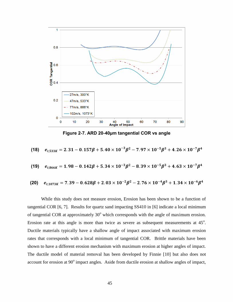
45
Figure 2-7. ARD 20-40µm tangential COR vs angle
(18) 𝒆𝒕,𝟓𝟑𝟑𝑲 = 𝟐. 𝟑𝟏 − 𝟎. 𝟏𝟓𝟕𝜷 + 𝟓. 𝟒𝟎 × 𝟏𝟎 𝟑𝜷𝟐 − 𝟕. 𝟗𝟕 × 𝟏𝟎 𝟓𝜷𝟑 + 𝟒. 𝟐𝟔 × 𝟏𝟎 𝟕𝜷𝟒
(19) 𝒆𝒕,𝟖𝟔𝟔𝑲 = 𝟏. 𝟗𝟖 − 𝟎. 𝟏𝟒𝟐𝜷 + 𝟓. 𝟑𝟒 × 𝟏𝟎 𝟑𝜷𝟐 − 𝟖. 𝟑𝟗 × 𝟏𝟎 𝟓𝜷𝟑 + 𝟒. 𝟔𝟑 × 𝟏𝟎 𝟕𝜷𝟒
(20) 𝒆𝒕,𝟏𝟎𝟕𝟑𝑲 = 𝟕. 𝟑𝟗 − 𝟎. 𝟔𝟐𝟖𝜷 + 𝟐. 𝟎𝟑 × 𝟏𝟎 𝟐𝜷𝟐 − 𝟐. 𝟕𝟔 × 𝟏𝟎 𝟒𝜷𝟑 + 𝟏. 𝟑𝟒 × 𝟏𝟎 𝟔𝜷𝟒
While this study does not measure erosion, Erosion has been shown to be a function of
tangential COR [6, 7]. Results for quartz sand impacting SS410 in [6] indicate a local minimum
of tangential COR at approximately 30o which corresponds with the angle of maximum erosion.
Erosion rate at this angle is more than twice as severe as subsequent measurements at 45o.
Ductile materials typically have a shallow angle of impact associated with maximum erosion
rates that corresponds with a local minimum of tangential COR. Brittle materials have been
shown to have a different erosion mechanism with maximum erosion at higher angles of impact.
The ductile model of material removal has been developed by Finnie [10] but also does not
account for erosion at 90o impact angles. Aside from ductile erosion at shallow angles of impact,

46
there is not much agreement in the literature over the erosion mechanisms at normal impact
angles or with brittle materials.
Unfortunately, quartz sand study [6] is the only study to look at both tangential COR and
erosion. In the current study, as seen in Figure 2-7, there is a relatively flat trend for ambient and
533oK (47m/s) and relatively flat trend with a distinct local minima at 68
o for the 866
oK (77m/s)
case. The 1073oK (102m/s) case also exhibits this minima but has an additional minima at
approximately 31o degree also. These may indicate the onset of erosion due to the higher
velocities for the microparticles impacting stainless steel, but further study is needed. The angle
of impact where the tangential COR begins to increase rapidly appears to shift to higher angles
of impact also. Future experiments documenting the relationship between tangential COR and
erosion would be beneficial in helping to predict the effects of particle ingestion at engine
realistic conditions.
2.6 Discussion on Temperature/Velocity Effects
The main source of energy loss during impact is the result of plastic deformation.
Dislocations and imperfections in the material are moved through the material, attempting to
distribute the impulse and find equilibrium during compression. At increased temperatures, the
atoms vibration amplitude increases, increasing the position between stable atom locations. This
leads to decreased bond strength in the material allowing dislocations in the crystal structure to
relocate with less force, thus increasing plastic deformation and reducing COR. However, the
effect of temperature of materials during a rapid impact is mostly un-documented, especially for
microparticles.
Many of the material property relationships that have been analytically developed, and
are available in sources such as Fischer-Cripps [17] for elastic-plastic impact, involve the ratio
E/Y, where E is the elastic modulus and Y is the Yield Strength. However, much of the
experimental rebound data does not exhibit a clear relationship between material properties of E,
Y or Hardness. The complex interplay between these changes in material properties over a rapid
impact event can prove very difficult to predict, model, and analyze. While the effects of
temperature on COR have not been documented, some empirical data has correlated COR to
changes in velocity. This is a useful starting point for looking at the temperature/velocity
conditions at impact in the VT Aerothermal Rig.

47
Various references [5, 18] have suggested that COR decreases proportionally with
velocity according to the equation
(21) 𝒆 = 𝒂𝒗 𝒃
where and are constants. These sources have shown to be related to the impact conditions
(i.e. materials, angle, etc.) and to be equal to ¼ for 90o impacts. It must be noted these did not
include oblique impacts, tangential rebound does not factor into these results. Similar variation
of the rebound velocity versus impact velocity at oblique angles was measured by Hutchings et.
al. [19] for hardened steel spheres impacting mild steel targets, however, tabulated data was not
available for accurate comparison with the current trends. This study, through the coupling of
temperature and velocity, obtains oblique COR measurements at different impact conditions and
attempts to quantify the relationship of COR and temperature using the existing knowledge on
the relationship of COR and velocity.
The next analysis in Figure 2-8 plots the total COR results for a few angles on the y-axis
versus velocity on the x-axis utilizing a log-log scale. The corresponding power law
relationships are also attached in Table 2-4. The overall trend in Table 2-4 showed a jump in
coefficient of determination (R2) at the 70 and 75 degree impact angle, however, the value also
decreases at these points. If this trend continues, it suggests that the power law relationship may
only exhibit satisfactory agreement (R2 ≈1) with experimental data at 90 degree angle. The
coefficient of determination indicates poor agreement from 40-60 degrees, where the 1073oK
(102m/s) COR vs angle trend line intersects the lower temperature/velocity cases as shown in
Figure 2-5. The trend is also of interest to this study because it does not appear to be anywhere
near the 0.25 value found in previous studies. The 0.25 value was found for metal spheres, larger
than 120μm, impacting metal plates whereas the current study has 20-40μm rough sand
impacting metal. This is very difficult to explain as there is no validation data for such small
particle impact at high temperature/velocity conditions. Theoretical analysis for such conditions
is limited in predictive behavior to evaluate baseline numbers to clarify the current dataset.

48
Figure 2-8. ARD 20-40µm COR vs Velocity
Table 2-4. Power Law curve fit parameters
Angle a b R2
25 1.3021 0.148 0.944
30 1.2074 0.143 0.954
35 1.1049 0.124 0.944
40 1.0074 0.124 0.889
45 0.9237 0.116 0.807
50 0.863 0.115 0.768
55 0.8221 0.122 0.798
60 0.7989 0.136 0.878
65 0.7814 0.152 0.947
70 0.7487 0.162 0.974
75 0.6678 0.147 0.975
The most relevant conclusion to this study to be taken from Figure 2-8, is that a drastic
reduction in COR was not measured at the highest temperature case. The reduction in COR in

49
the VT Aerothermal rig at elevated temperature and velocity conditions does not exceed the
expected reduction due to velocity increase alone. For a convincing argument that increasing
temperature plays a significant role in the decrease of COR, an increase in the power law
exponent (the exponent attributed to velocity changes) would need to correlate to the
experimental data at higher temperature/velocity. Looking at the data in two groups the value
does not shift in a significant way going from 533oK to 866
oK or from 866
oK to 1073
oK .
Further rational for the lack of temperature effect is presented here. It has been shown by
a number of researchers studying deposition that above a critical temperature, particles begin to
stick to the impacting surface. In this work, deposition can be interpreted as a special case,
where COR = 0, a perfectly plastic collision. The critical temperature was determined by Crosby
et. al. [20] to be 1233oK for 3μm coal ash which had approximately 47.4% Si by weight. Above
the critical temperature, deposition increased exponentially. This is in agreement with the
computational model developed by Sreedharan and Tafti [21] that bases deposition on critical
viscosity. Particles below the softening temperature still had a sticking probability for any
impact with the surface. This study showed that impact behavior had an exponential
relationship, changing drastically and significantly, above a critical temperature.
In the absence of an exponential or a drastic change in trend, a more subtle change was
hypothesized. Substituting temperature for velocity and using a similar power law relationship
to that in (21), the mean total COR can be extrapolated at higher temperatures. At 1363oK (the
100% melting point of ARD [15]) the mean COR is predicted to be 0.32 at a 75 degree angle of
impact. The literature suggests that deposition would occur at this temperature leading to a mean
total COR very near zero. These conclusions taken together led the researchers to believe a
significant deviation from the power law relationship would occur rather sharply above a critical
temperature that was not reached in this study.
The reduction in elastic modulus and yield strength of the steel, along with the material
changes in the ARD, were expected to play a larger part in the impact mechanics, however,
further study at higher temperatures is needed for a comprehensive understanding of the physics
involved just prior to deposition.
The impact physics are further investigated in Figure 2-9 and Figure 2-10 where Normal
and Tangential COR are presented versus impact velocity. Figure 2-9 shows that normal COR,
above 60o impact angle follows a very similar trend with respect to impact velocity. However,

50
lower angles begin to increasingly deviate, for example the trend at 30o impact angle is also
shown. At angles of impact higher than 60o, total COR is primarily determined by the
mechanism of normal impact energy dissipation, plastic deformation. Imperfections in the
material are permanently relocated through the material structure to dissipate impact energy.
Figure 2-9. Normal COR vs Normal Impact Velocity
Figure 2-10 shows the relationship for Tangential COR. Tangential COR shows a very
similar trend for angles of impact less than 45o, at higher angles the trend deviates as shown by
the 75o impact angle data. At angles of impact less than 45
o, tangential impact velocity
dominates and total COR is primarily determined by the tangential mechanisms of energy
dissipation. The main mechanism is friction as the particle briefly slides along the surface during
the contact duration. In the region between 45 and 60 degrees the energy dissipation
mechanisms compete and the COR takes on an intermediate value.

51
Figure 2-10. Tangential COR vs Tangential Impact Velocity
Attempts were made to normalize the existing data for comparison due to lack of
experimental research under engine representative impact events. In Figure 2-11, COR at a
given angle was plotted on a log-log scale against average incoming particle kinetic energy (KE).
Data from Tabakoff et al. [8, 9] was included to see if the velocity and size differences between
experiments could be mitigated. The KE of the fly ash data fell in between the ambient and
533oK data set, the sand data had a much higher KE. Qualitatively, it appears a smooth
relationship between COR and KE exists. However, it did not hold a power law relationship, thus
COR must scale differently with mass/material properties. This exercise, while informative, did
not lead to an overall correlation between COR and KE. There were not enough points to
satisfactorily determine a polynomial relationship without directly solving for coefficients.
Developing a universal relationship for COR with engine realistic impact conditions would be a
major breakthrough in the study of particle ingestion effects.

52
Figure 2-11. ARD 20-40µm COR vs KE (½mv2)
The discussed work begins to document uninvestigated areas of impact research.
Oblique impacts at high temperature have only been documented with respect to the deposits
formed or material removed. Previous normal impacts experiments at high temperature involve
materials and sizes that are not engine representative. The empirical correlations developed here
can be readily integrated into commercial CFD code. When run on engine geometry, the
subsequent modeling of impact and re-entrainment into the flow can predict areas susceptible to
erosion in secondary flows and accurate particle trajectories exiting cooling channels into hot gas
paths. Without accurate COR data, particle transport after the initial impact will not be
accurately modeled. This dataset provides engine realistic experiments documenting COR and
particle rebound behavior.
2.7 Conclusions
Datasets at engine realistic particle size and temperature were presented at different angles
and velocities for microparticle sand impacting 304 Stainless Steel. The data presented here is
intended to provide an estimate of both the mean and variance expected from an impact of these
specific materials at a given angle, temperature, and velocity, which has not been presented in
53
prior gas turbine literature. The data from the present study indicated that the power law
relationship with velocity may only be satisfied at impact angles equal to 90o while the
coefficients are determined experimentally for different impact conditions. Experimental results
presented at 533oK (47m/s), 866
oK (77m/s), and 1073
oK (102m/s) show that COR is reduced by
an average of 12%, 15%, and 16% respectively over ambient baseline results. This is attributed
primarily to the increase in velocity that is coupled to the temperature increase in the VT
Aerothermal Rig. Temperatures up to 1073oK do not appear to significantly reduce COR, as has
been witnessed at higher temperatures where plastic collisions can result in deposition.
2.8 Acknowledgments
The co-authors on this paper are are J.M. Delimont, W.F. Ng, S.V. Ekkad from Virinia
Tech, Blacksburg, VA, USA. An abstract containing this work will be submitted to ASME IGTI
Turbo Expo by August 27, 2012 followed by journal submission to the appropriate publication.
The final paper will incorporate some of the suggestions for future work discussed in this paper,
carried out by the co-authors.
The work detailed here would not be possible without the support and direction of Rolls-
Royce, Indianapolis, IN. The authors would also like to thank D.K. Tafti and S. Singh from
Virginia Tech for their thoughtful discussion, analysis and advice.
2.9 References
[1] Goldsmith, W., 2002, Impact : the theory and physical behaviour of colliding solids, Dover
Publications, Mineola, N.Y.
[2] Armstrong, J. D., Collings, N., and Shayler, P.J., 1984, "Trajectory of Particles Rebounding
Off Plane Targets," AIAA, 22(2), pp. 214-218.
[3] Sommerfeld, M., and Huber, N., 1999, "Experimental analysis and modelling of particle-wall
collisions," International Journal of Multiphase Flow, 25, pp. 1457-1489.
[4] Mok, C. H., and Duffy, J., 1964, "THE BEHAVIOUR OF METALS AT ELEVATED
TEMPERATURES UNDER IMPACT WITH A BOUNCING BALL," Int J Mech Sci, 6, pp.
161-175.
[5] Brenner, S. S., Wriedt, H. A., and Oriani, R. A., 1981, "Impact adhesion of iron at elevated
temperatures," Wear, 68(2), pp. 169-190.
[6] Tabakoff, W., Grant, G., and Ball, R., 1974, "An Experimental Investigation of Certain
Aerodynamic Effects on Erosion," AIAA-74-639.
[7] Grant, G., and Tabakoff, W., 1975, "Erosion Prediction in Turbomachinery Resulting from
Environmental Solid Particles," J. Aircraft, 12(5), pp. 471-478.
[8] Tabakoff, W., 1991, "Measurements of Particles Rebound Characteristics on Materials Used
in Gas Turbines," J. of Propulsion and Power, 7(5), pp. 805-813.

54
[9] Tabakoff. W, H., A., and Murugan, D.M, 1996, "Effect of Target Materials on the Particle
Restitution Characteristics for Turbomachinery Application," J. of Propulsion and Power, 12(2),
pp. 260-266.
[10] Finnie, I., 1960, "Erosion of surfaces by solid particles," Wear, 3(2), pp. 87-103.
[11] Wakeman, T., and Tabakoff, W., 1979, "Erosion Behavior in a Simulated Jet Engine
Environment," J. Aircraft, 16(12), pp. 828-833.
[12] Hylton, L., Nirmalan, V., Sultanian, B., Kaufman, R., 1988, "The Effects of Leading Edge
and Downstream Film Cooling on Turbine Vane Heat Transfer," NASA Contractor Report
182133.
[13] Nealy, D., Mihelc, M., Hylton, L., Gladden, H., 1984, "Measurements of Heat Transfer
Distribution Over the Surfaces of Highly Loaded Turbine Nozzle Guide Vanes," Journal of
Engineering for Gas Turbines and Power, 106, pp. 149-158.
[14] Reagle, C. J., Delimont, J.M., Ng, W.F., and Ekkad, S.V., 2012, "A NOVEL TECHNIQUE
FOR MEASURING THE COEFFICIENT OF RESTITUTION OF MICROPARTICLE
IMPACTS IN A FORCED FLOWFIELD," GT2012-68252.
[15] Walsh, W. S., Thole, K. A., and Joe, C., 2006, "Effects of Sand Ingestion on the Blockage
of Film-Cooling Holes," ASME Conference Proceedings, 2006(4238X), pp. 81-90.
[16] Schairer, J. F., and Bowen, N.L., 1947, "Melting Relations in the systems Na2O-Al2-O3-
SiO2 and K2O-Al2-O3-SiO2," American Journal of Science, 245(4), pp. 193-204.
[17] Fischer-Cripps, A. C., 2000, Introduction to Contact Mechanics, Springer.
[18] Johnson, K. L., 1985, Contact Mechanics, Cambridge University Press, Cambridge, UK.
[19] Hutchings, I. M., Macmillan, N. H., and Rickerby, D. G., 1981, "Further studies of the
oblique impact of a hard sphere against a ductile solid," International Journal of Mechanical
Sciences, 23(11), pp. 639-646.
[20] Crosby, J. M., Lewis, S., Bons, J. P., Ai, W., and Fletcher, T. H., 2008, "Effects of
Temperature and Particle Size on Deposition in Land Based Turbines," Journal of Engineering
for Gas Turbines and Power, 130(5), p. 051503.
[21] Sreedharan, S. S., and Tafti, D. K., 2011, "Composition dependent model for the prediction
of syngas ash deposition in turbine gas hotpath," International Journal of Heat and Fluid Flow,
32(1), pp. 201-211.
55
Conclusions and Future Work
In the preface, an overall picture of the research to be completed was presented. It was
intended to focus the reader to the significance of each individual paper. In this section, the
combined conclusions of the work will be presented along with a discussion on future work.
This work was conducted in an attempt to quantify for the project sponsors, particle
bounce back in gas turbine engine environments. Data for sand and dust with realistic size and
chemical composition is measured at ambient temperature with limited impact conditions.
Coefficient of Restitution data in published literature at high temperature is not representative of
sand and dust actually ingested into engines. Experimental information is needed for specific
materials, impact velocity, and impact angle to predict particle rebound behavior. A general
correlation that includes these variables does not exist. Rebound correlations are useful for
engine designers such as Rolls-Royce looking to analyze particle transport in realistic
geometries. Analysis of engine hardware can identify areas susceptible to erosion and deposition
leading to improved performance and longevity of gas turbines operating in particulate laden
environments.
A major obstacle to particle transport analysis is actually measuring particle rebound in
an engine realistic environment to incorporate into the model. In the first paper, a hybrid
PTV/CFD technique for measuring microparticle COR was presented and validated. Data from
particles entrained in a 27m/s free jet impacting 304 Stainless Steel was presented at different
angles. The glass bead data provided a large, smooth, spherical particle test case for comparison
with literature. The data from the 10-20μm ARD proved to be in qualitative and quantitative
agreement with literature and the 20-40μm ARD test case, however, the data had significantly
more noise than the latter test case. Results for mean total, tangential, and normal COR were
shown and empirical polynomial correlations condensing over 13,000 individual impacts were
presented. The results are in qualitative and quantitative agreement with past experiments for
microparticles at similar, but not identical, sizes, angles, and velocities. The agreement of the
resulting data with that of published literature using different measurement techniques has
validated the hybrid PTV/CFD technique. The data is of acceptable quality and can be obtained
with economical, readily-available hardware and software. The dataset from this experiment
also completes the understanding of COR behavior for sand particles under 40μm when
compared to available literature that is limited to particle sizes above 100μm.
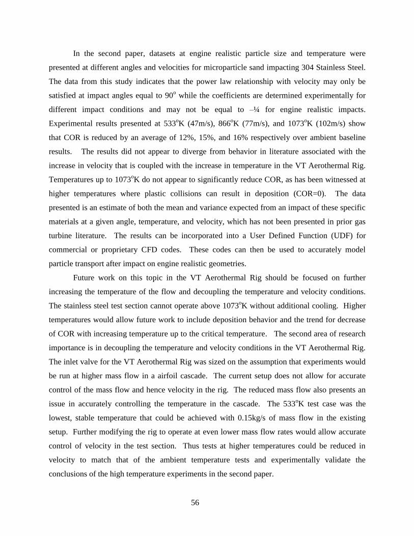
56
In the second paper, datasets at engine realistic particle size and temperature were
presented at different angles and velocities for microparticle sand impacting 304 Stainless Steel.
The data from this study indicates that the power law relationship with velocity may only be
satisfied at impact angles equal to 90o while the coefficients are determined experimentally for
different impact conditions and may not be equal to –¼ for engine realistic impacts.
Experimental results presented at 533oK (47m/s), 866
oK (77m/s), and 1073
oK (102m/s) show
that COR is reduced by an average of 12%, 15%, and 16% respectively over ambient baseline
results. The results did not appear to diverge from behavior in literature associated with the
increase in velocity that is coupled with the increase in temperature in the VT Aerothermal Rig.
Temperatures up to 1073oK do not appear to significantly reduce COR, as has been witnessed at
higher temperatures where plastic collisions can result in deposition (COR=0). The data
presented is an estimate of both the mean and variance expected from an impact of these specific
materials at a given angle, temperature, and velocity, which has not been presented in prior gas
turbine literature. The results can be incorporated into a User Defined Function (UDF) for
commercial or proprietary CFD codes. These codes can then be used to accurately model
particle transport after impact on engine realistic geometries.
Future work on this topic in the VT Aerothermal Rig should be focused on further
increasing the temperature of the flow and decoupling the temperature and velocity conditions.
The stainless steel test section cannot operate above 1073oK without additional cooling. Higher
temperatures would allow future work to include deposition behavior and the trend for decrease
of COR with increasing temperature up to the critical temperature. The second area of research
importance is in decoupling the temperature and velocity conditions in the VT Aerothermal Rig.
The inlet valve for the VT Aerothermal Rig was sized on the assumption that experiments would
be run at higher mass flow in a airfoil cascade. The current setup does not allow for accurate
control of the mass flow and hence velocity in the rig. The reduced mass flow also presents an
issue in accurately controlling the temperature in the cascade. The 533oK test case was the
lowest, stable temperature that could be achieved with 0.15kg/s of mass flow in the existing
setup. Further modifying the rig to operate at even lower mass flow rates would allow accurate
control of velocity in the test section. Thus tests at higher temperatures could be reduced in
velocity to match that of the ambient temperature tests and experimentally validate the
conclusions of the high temperature experiments in the second paper.
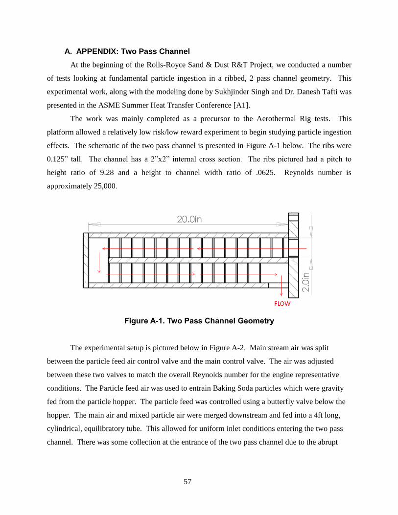
57
A. APPENDIX: Two Pass Channel
At the beginning of the Rolls-Royce Sand & Dust R&T Project, we conducted a number
of tests looking at fundamental particle ingestion in a ribbed, 2 pass channel geometry. This
experimental work, along with the modeling done by Sukhjinder Singh and Dr. Danesh Tafti was
presented in the ASME Summer Heat Transfer Conference [A1].
The work was mainly completed as a precursor to the Aerothermal Rig tests. This
platform allowed a relatively low risk/low reward experiment to begin studying particle ingestion
effects. The schematic of the two pass channel is presented in Figure A-1 below. The ribs were
0.125” tall. The channel has a 2”x2” internal cross section. The ribs pictured had a pitch to
height ratio of 9.28 and a height to channel width ratio of .0625. Reynolds number is
approximately 25,000.
Figure A-1. Two Pass Channel Geometry
The experimental setup is pictured below in Figure A-2. Main stream air was split
between the particle feed air control valve and the main control valve. The air was adjusted
between these two valves to match the overall Reynolds number for the engine representative
conditions. The Particle feed air was used to entrain Baking Soda particles which were gravity
fed from the particle hopper. The particle feed was controlled using a butterfly valve below the
hopper. The main air and mixed particle air were merged downstream and fed into a 4ft long,
cylindrical, equilibratory tube. This allowed for uniform inlet conditions entering the two pass
channel. There was some collection at the entrance of the two pass channel due to the abrupt
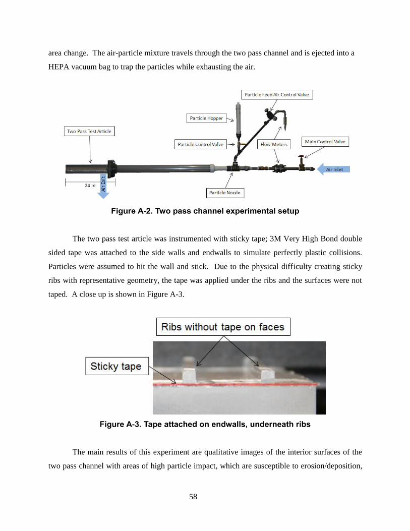
58
area change. The air-particle mixture travels through the two pass channel and is ejected into a
HEPA vacuum bag to trap the particles while exhausting the air.
Figure A-2. Two pass channel experimental setup
The two pass test article was instrumented with sticky tape; 3M Very High Bond double
sided tape was attached to the side walls and endwalls to simulate perfectly plastic collisions.
Particles were assumed to hit the wall and stick. Due to the physical difficulty creating sticky
ribs with representative geometry, the tape was applied under the ribs and the surfaces were not
taped. A close up is shown in Figure A-3.
Figure A-3. Tape attached on endwalls, underneath ribs
The main results of this experiment are qualitative images of the interior surfaces of the
two pass channel with areas of high particle impact, which are susceptible to erosion/deposition,
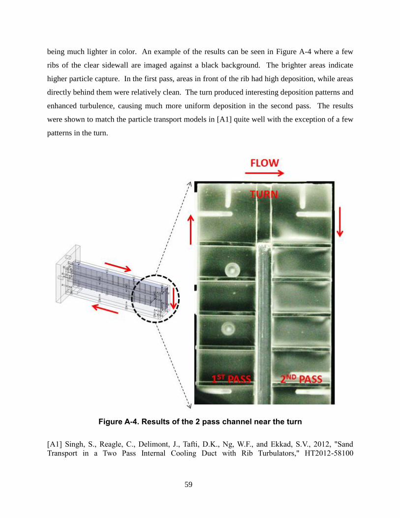
59
being much lighter in color. An example of the results can be seen in Figure A-4 where a few
ribs of the clear sidewall are imaged against a black background. The brighter areas indicate
higher particle capture. In the first pass, areas in front of the rib had high deposition, while areas
directly behind them were relatively clean. The turn produced interesting deposition patterns and
enhanced turbulence, causing much more uniform deposition in the second pass. The results
were shown to match the particle transport models in [A1] quite well with the exception of a few
patterns in the turn.
Figure A-4. Results of the 2 pass channel near the turn
[A1] Singh, S., Reagle, C., Delimont, J., Tafti, D.K., Ng, W.F., and Ekkad, S.V., 2012, "Sand
Transport in a Two Pass Internal Cooling Duct with Rib Turbulators," HT2012-58100
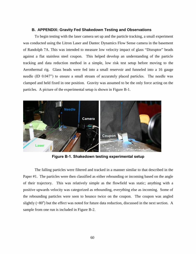
60
B. APPENDIX: Gravity Fed Shakedown Testing and Observations
To begin testing with the laser camera set up and the particle tracking, a small experiment
was conducted using the Litron Laser and Dantec Dynamics Flow Sense camera in the basement
of Randolph 7A. This was intended to measure low velocity impact of glass “Disruptor” beads
against a flat stainless steel coupon. This helped develop an understanding of the particle
tracking and data reduction method in a simple, low risk test setup before moving to the
Aerothermal rig. Glass beads were fed into a small reservoir and funneled into a 16 gauge
needle (ID 0.047”) to ensure a small stream of accurately placed particles. The needle was
clamped and held fixed in one position. Gravity was assumed to be the only force acting on the
particles. A picture of the experimental setup is shown in Figure B-1.
Figure B-1. Shakedown testing experimental setup
The falling particles were filtered and tracked in a manner similar to that described in the
Paper #1. The particles were then classified as either rebounding or incoming based on the angle
of their trajectory. This was relatively simple as the flowfield was static; anything with a
positive upwards velocity was categorized as rebounding, everything else as incoming. Some of
the rebounding particles were seen to bounce twice on the coupon. The coupon was angled
slightly (~80o) but the effect was noted for future data reduction, discussed in the next section. A
sample from one run is included in Figure B-2.

61
Figure B-2. Particle tracks and classification from Shakedown testing
At this point it is worth noting a few of the interesting behaviors witnessed in the
shakedown testing that were translated to the VT Aerothermal Rig during the forced flowfield
testing.
Incoming/Rebounding particles in VT Aerothermal Rig
The first step after particle tracking is to sort the particles into either the rebounding or
incoming category. This is accomplished based on the angle of the coupon and the measured
trajectory angle of the particle. Particles with a trajectory towards the coupon are put in the
incoming category for forward tracking. Particles with an angle away from the coupon face are
labeled rebounding particles and will be tracked backwards in the algorithm described in the
technique paper. The trajectory angle is used because there is essentially no way for a particle
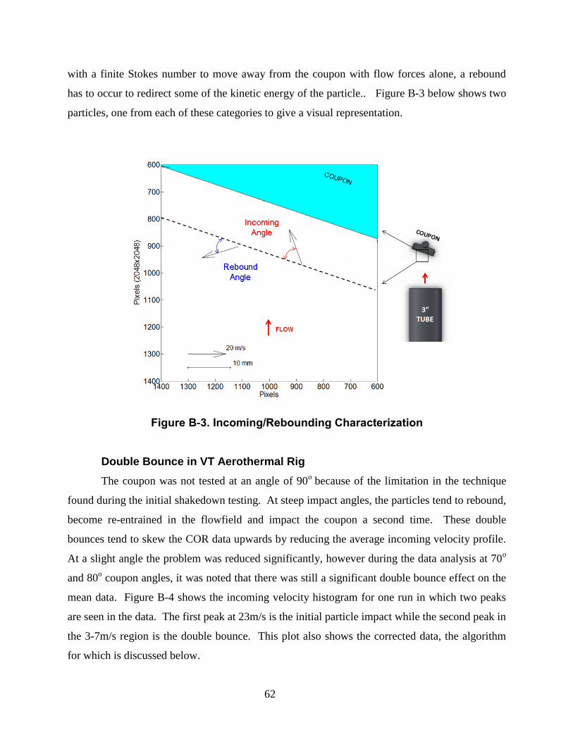
62
with a finite Stokes number to move away from the coupon with flow forces alone, a rebound
has to occur to redirect some of the kinetic energy of the particle.. Figure B-3 below shows two
particles, one from each of these categories to give a visual representation.
Figure B-3. Incoming/Rebounding Characterization
Double Bounce in VT Aerothermal Rig
The coupon was not tested at an angle of 90o
because of the limitation in the technique
found during the initial shakedown testing. At steep impact angles, the particles tend to rebound,
become re-entrained in the flowfield and impact the coupon a second time. These double
bounces tend to skew the COR data upwards by reducing the average incoming velocity profile.
At a slight angle the problem was reduced significantly, however during the data analysis at 70o
and 80o coupon angles, it was noted that there was still a significant double bounce effect on the
mean data. Figure B-4 shows the incoming velocity histogram for one run in which two peaks
are seen in the data. The first peak at 23m/s is the initial particle impact while the second peak in
the 3-7m/s region is the double bounce. This plot also shows the corrected data, the algorithm
for which is discussed below.
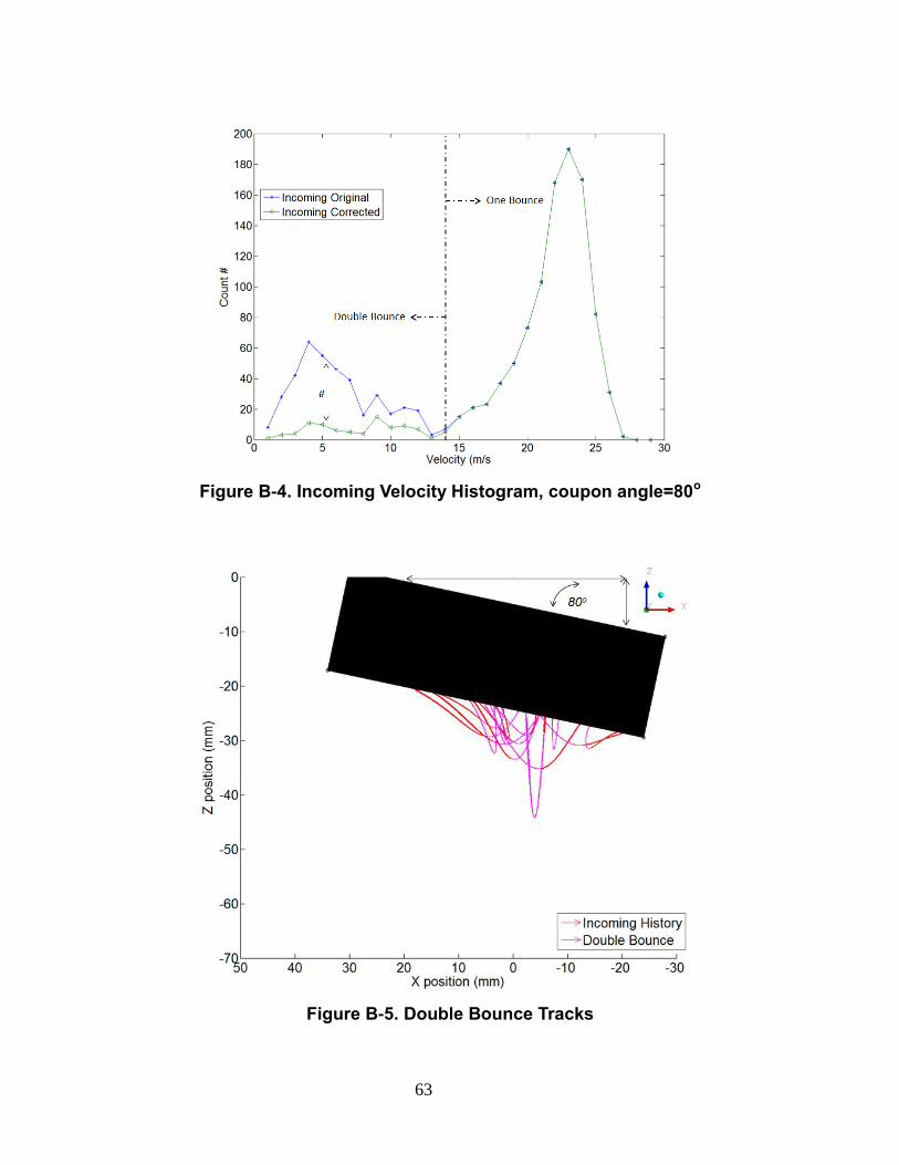
63
Figure B-4. Incoming Velocity Histogram, coupon angle=80o
Figure B-5. Double Bounce Tracks
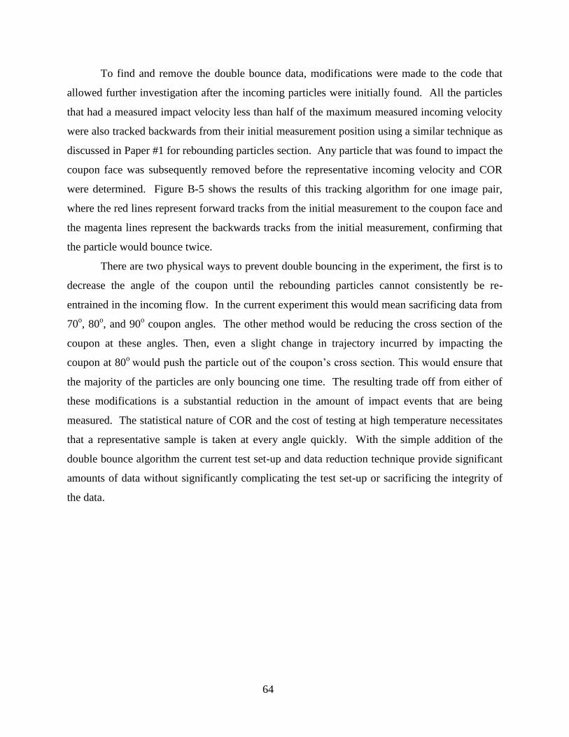
64
To find and remove the double bounce data, modifications were made to the code that
allowed further investigation after the incoming particles were initially found. All the particles
that had a measured impact velocity less than half of the maximum measured incoming velocity
were also tracked backwards from their initial measurement position using a similar technique as
discussed in Paper #1 for rebounding particles section. Any particle that was found to impact the
coupon face was subsequently removed before the representative incoming velocity and COR
were determined. Figure B-5 shows the results of this tracking algorithm for one image pair,
where the red lines represent forward tracks from the initial measurement to the coupon face and
the magenta lines represent the backwards tracks from the initial measurement, confirming that
the particle would bounce twice.
There are two physical ways to prevent double bouncing in the experiment, the first is to
decrease the angle of the coupon until the rebounding particles cannot consistently be re-
entrained in the incoming flow. In the current experiment this would mean sacrificing data from
70o, 80
o, and 90
o coupon angles. The other method would be reducing the cross section of the
coupon at these angles. Then, even a slight change in trajectory incurred by impacting the
coupon at 80o
would push the particle out of the coupon’s cross section. This would ensure that
the majority of the particles are only bouncing one time. The resulting trade off from either of
these modifications is a substantial reduction in the amount of impact events that are being
measured. The statistical nature of COR and the cost of testing at high temperature necessitates
that a representative sample is taken at every angle quickly. With the simple addition of the
double bounce algorithm the current test set-up and data reduction technique provide significant
amounts of data without significantly complicating the test set-up or sacrificing the integrity of
the data.

65
C. APPENDIX: Sensitivity and Uncertainty
To analyze how errors in the CFD may introduce errors into the COR, a sensitivity
analysis was conducted. The results of this analysis are discussed in Paper #1 and are presented
in detail here.
The CFD was initially matched to the Pitot-Static traverse data presented in Figure 1-3.
The inlet velocity matched quite well in the projected area of the coupon. The idea was to
introduce an error into the CFD and measure the response of a representative dataset. The CFD
results were artificially increased 15%, meaning every U and W vector was scaled up by 15%.
While not physically similar to increasing the mass flow out of the pipe by 15%, it presented a
worst case scenario that was quick and easy to implement. The result of reducing the particle
measurements using the scaled data is presented in Figure C-1. The average error was 6.8%.
The highest errors were from angle of impact 26-49 degrees, where the average error was greater
than 9%. Errors were under 3% from 75-84 degrees.
Figure C-1. Ambient Sensitivity to CFD Data
To verify that the errors introduced by scaling the CFD data were reasonable, two CFD
cases were re-run and the inlet total pressure increased so that the velocity exiting the tube was
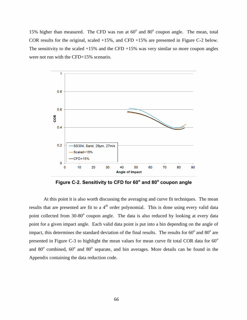
66
15% higher than measured. The CFD was run at 60o and 80
o coupon angle. The mean, total
COR results for the original, scaled +15%, and CFD +15% are presented in Figure C-2 below.
The sensitivity to the scaled +15% and the CFD +15% was very similar so more coupon angles
were not run with the CFD+15% scenario.
Figure C-2. Sensitivity to CFD for 60o and 80o coupon angle
At this point it is also worth discussing the averaging and curve fit techniques. The mean
results that are presented are fit to a 4th
order polynomial. This is done using every valid data
point collected from 30-80o coupon angle. The data is also reduced by looking at every data
point for a given impact angle. Each valid data point is put into a bin depending on the angle of
impact, this determines the standard deviation of the final results. The results for 60o and 80
o are
presented in Figure C-3 to highlight the mean values for mean curve fit total COR data for 60o
and 80o combined, 60
o and 80
o separate, and bin averages. More details can be found in the
Appendix containing the data reduction code.

67
Figure C-3. Curve fitting, local, and global averaging
68
D. APPENDIX: Particle Delivery System
Delivering the particles during these experiments was not a trivial matter. There are a
number of elaborate methods involving roller cams, plungers, etc. that have been used in
literature, but it is usually mentioned as an afterthought with no discussion of the difficulties
associated with delivering particles into the test section. To simply deliver particles into a test
section was relatively simple. To do so consistently with respect to time and material was not.
To find a system that would work for this setup took much iteration.
After examining the alternatives, a relatively simple design was decided upon, similar to
a sand blaster. A portion of the mainstream air was diverted into a secondary flow path. Along
this flow path sat a storage hopper with a valve on the outlet. The particles were released by
partially opening the valve, allowing gravity and flow pressure difference to entrain the particles
into the airstream. However, continuous flow and consistent particle amounts were not achieved.
It was from this baseline that attempts were made to improve the design.
The tubing was reduced in size from ½” to ¼” to reduce the amount of sand delivered per
experiment. However, the consistency of baking soda was negatively affected. The airflow
tubing was increased back to ½”, while the hopper wye junction was kept at ¼” to create a
Venturi effect underneath the hopper. This helped draw the particles into the flow while still
delivering a smaller amount each time. An adjustable pressure regulator was attached to provide
greater control over the airstream. Globe, Ball and Butterfly valves were all tested to control the
flow of particles from the hopper, with the Butterfly valve having the best results. Mike Fertall
ran many of these tests, quantifying the delivering characteristics and rates of each iteration.
This design was optimized for ejecting baking soda particles from the blaster. The design
was fairly consistent and sufficient for initial tests. This setup was used for the 2 pass channel
experiment shown in Figure A-2 and worked quite well with baking soda. However, as the 2
pass channel tests started to converge with the related CFD work and actual engine conditions,
Arizona Road Dust replaced baking soda in the blaster.
This created an entirely new set of issues with particle delivery. Where the baking soda
particle was designed for just this sort of application, blasting a surface with an air/baking soda
mix to clean it, the sand particles tended to eject in bursts and would often get stuck in
suspension in the hopper, requiring agitation to continue flowing.
69
The test dust also has a finite size distribution. The larger and less densely packed the
particles, the more voids present. These voids allow the non-spherical particles to flow and
move as particles feed into the system. When relatively small particles are present, they fill these
voids and inhibit particle flow. These suspensions require constant agitation to achieve
continuous flow.
The first design modification was to pressurize the hopper from the top down. The
smaller dust particles were not gravity feeding, but actually collecting in the top of the hopper.
Adding additional hoses and eventually another adjustable pressure regulator greatly improved
sand delivery, even allowing for continuous flow of particles. However, as initial Particle
Tracking Velocimetry (PTV) measurements were made in the Aerothermal Rig, the amount of
particles being delivered became an issue. The particle seeding was simply too dense. To
decrease the amount, the hopper valve was shut further; this inhibited continuous particle flow
and required manual agitation, i.e. hitting the steel hopper with a 13mm wrench.
For ambient testing this produced satisfactory results with reasonable, though not ideal,
repeatability. However, for safety reasons, when the burner is lit, no one can be present to
agitate the blaster. The solution came in the form of a pneumatic vibrator spinning at 15,000+
rpm and applying 20+ lbf to the hopper. The vibrator could be turned on remotely using a
CompactDAQ current output module, solid state relay, and solenoid valve. The blaster became
much more sensitive to opening angle. This was rectified by setting it with a feeler gauge to
within 0.001”. The current setup is displayed below in Figure D-1.

70
Figure D-1. Remote Particle Delivery System

71
E. APPENDIX: Traverse Design
Since a manual survey would be inherently unsafe in a high temperature environment, a
traverse was specified and designed that could characterize the inlet flow.
The design of the traverse was complicated by a number of factors. First and foremost,
the traverse was required to withstand extreme temperatures. The sealing and alignment issues
of the probes had to be addressed while ensuring relatively simple modifications to the test
section. Both probes needed to have enough travel that they could be moved entirely out of the
flow path when not in use so that they would not distort the flowfield upstream of the coupon or
become damaged by impinging particles.
An existing 300#, 4” Flange was modified to provide access, sealing, and mounting for
the traverse assembly. A Velmex, Inc. 8” XSlide® (XN10-0080-E01-71) was purchased along
with Automation Direct SureStep™ Stepping System including a NEMA 17 Motor, 4A Power
Supply, and Stepper Drive. The traverse system has 8” of travel and can hold a custom pitot-
static probe, designed to withstand almost 1100oC at the tip or a high temperature K type
thermocouple probe rated over 980oC based on the exposed wire diameter. Graphite Packing
Cord was used to seal the access hole around the probe. The custom parts were all made in
house at the Mechanical Engineering Machine Shop.
The entire traverse support needed to be mounted on a single flange. The probe was
located as far forward of the coupon as possible so the probe would not contact the coupon face
when the angle was changed. However, the probe could not be mounted so far forward that the
mounting bracket contacted the flange mounting bolts or the probe contacted the inner wall of
the short 4” tube leading to the test section. The Pitot-static probe can be successfully traversed
at coupon angles from 60-90o before contacting the edge of the coupon. The Pitot-static probe, to
satisfy the high temperature requirements had fixed take offs requiring a more complicated, thick
wall insertion. The straight, ¼” diameter thermocouple probe mounting was relatively simple,
compared to the Pitot-static probe. A small ledge at the bottom of a tapped hole was machined
to hold and compress the graphite packing when the probes were installed. A model of the
physical components is shown below in Figure E-1.
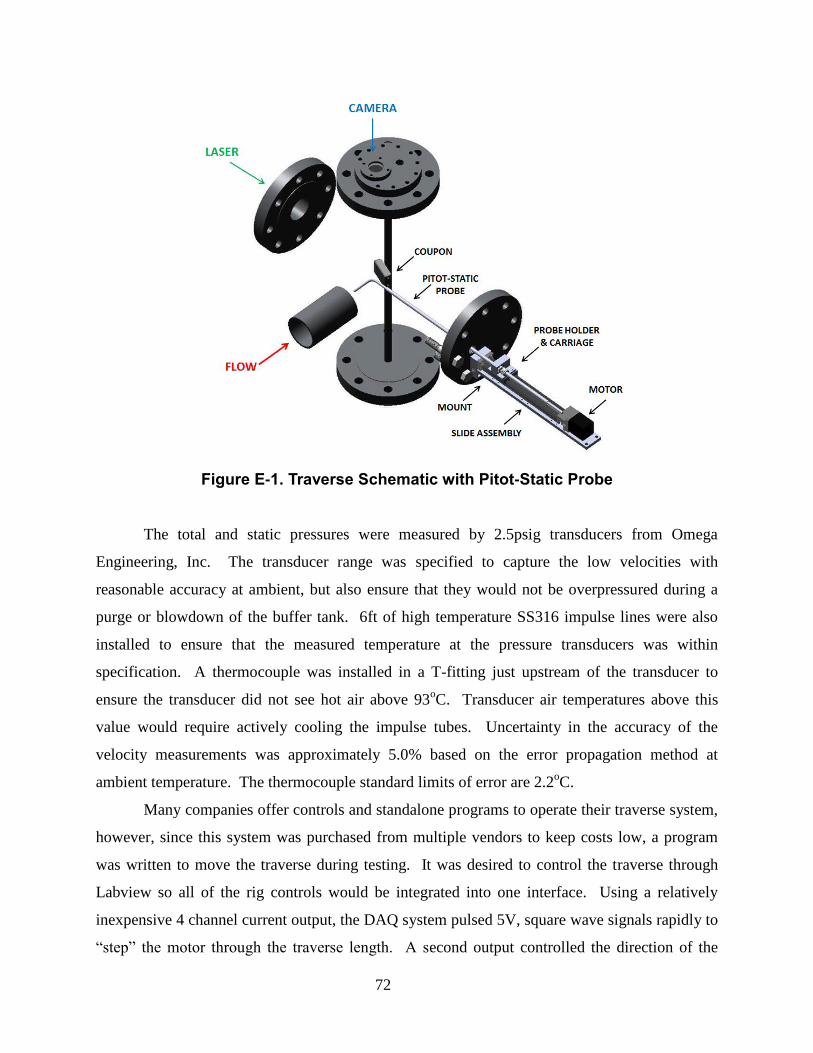
72
Figure E-1. Traverse Schematic with Pitot-Static Probe
The total and static pressures were measured by 2.5psig transducers from Omega
Engineering, Inc. The transducer range was specified to capture the low velocities with
reasonable accuracy at ambient, but also ensure that they would not be overpressured during a
purge or blowdown of the buffer tank. 6ft of high temperature SS316 impulse lines were also
installed to ensure that the measured temperature at the pressure transducers was within
specification. A thermocouple was installed in a T-fitting just upstream of the transducer to
ensure the transducer did not see hot air above 93oC. Transducer air temperatures above this
value would require actively cooling the impulse tubes. Uncertainty in the accuracy of the
velocity measurements was approximately 5.0% based on the error propagation method at
ambient temperature. The thermocouple standard limits of error are 2.2oC.
Many companies offer controls and standalone programs to operate their traverse system,
however, since this system was purchased from multiple vendors to keep costs low, a program
was written to move the traverse during testing. It was desired to control the traverse through
Labview so all of the rig controls would be integrated into one interface. Using a relatively
inexpensive 4 channel current output, the DAQ system pulsed 5V, square wave signals rapidly to
“step” the motor through the traverse length. A second output controlled the direction of the
73
motor using a 5V logic signal. Position was calibrated based on the number of square wave
signals sent to the motor. This was checked and initialized using the electric limit switches
attached to the slide assembly. The limit switches were plugged into the voltage measuring
module on the DAQ along with a 10kΩ “pull-up” resistor.
The only issue with the current setup is the lack of speed control. The traverse moved
speedily enough during the development phase of testing, however, when incorporated into a
program with many other measurements, issues arose. The Nyquist frequency forced an issue
with our DAQ system in which the sampling frequency had to be raised in order to speed up the
traverse. However, this led to a redundancy of data being taken over the entire test period which
was unacceptable for analysis and processing. Attempts to vary the sampling frequencies within
each DAQ Assistant VI caused Labview to spew forth random errors related to A/D conversion.
With the current programmer’s lack of sophistication, a good enough approach was taken in
which a single traverse travelling 5.28” requires approximately 8 minutes and 46 seconds. This
does however allow for many measurements over the traverse span. This issue will be
investigated with more time and resources.
Results from the Pitot-Static Surveys are presented in the attached papers in Figure 1-3
and Figure 2-3. The results from the thermocouple survey are presented in Figure 2-4. This
survey was presented as a temperature ratio. Due to operating issues in the tunnel, variations
were inevitable in the rig during the 8 minute long traverse movement. To determine if these
were the result of non-uniformities in the impinging flow or normal operation fluctuations, the
data from the thermocouple probe was normalized with a stationary thermocouple probe
downstream of the coupon. This resulted in a relatively flat velocity profile which was not
assumed to significantly affect the results. An image of the TC probe being traversed just in
front of the coupon is shown in Figure E-2.

74
Figure E-2. Laser-Camera image of TC Probe in front of coupon
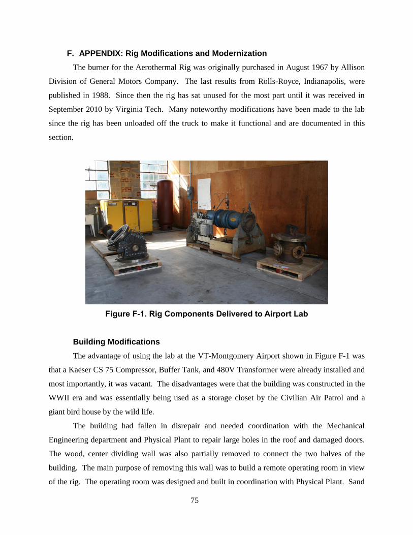
75
F. APPENDIX: Rig Modifications and Modernization
The burner for the Aerothermal Rig was originally purchased in August 1967 by Allison
Division of General Motors Company. The last results from Rolls-Royce, Indianapolis, were
published in 1988. Since then the rig has sat unused for the most part until it was received in
September 2010 by Virginia Tech. Many noteworthy modifications have been made to the lab
since the rig has been unloaded off the truck to make it functional and are documented in this
section.
Figure F-1. Rig Components Delivered to Airport Lab
Building Modifications
The advantage of using the lab at the VT-Montgomery Airport shown in Figure F-1 was
that a Kaeser CS 75 Compressor, Buffer Tank, and 480V Transformer were already installed and
most importantly, it was vacant. The disadvantages were that the building was constructed in the
WWII era and was essentially being used as a storage closet by the Civilian Air Patrol and a
giant bird house by the wild life.
The building had fallen in disrepair and needed coordination with the Mechanical
Engineering department and Physical Plant to repair large holes in the roof and damaged doors.
The wood, center dividing wall was also partially removed to connect the two halves of the
building. The main purpose of removing this wall was to build a remote operating room in view
of the rig. The operating room was designed and built in coordination with Physical Plant. Sand

76
filled cinder blocks were used to construct the walls and a high-impact window to safely view
the rig during operation. A high temperature steel exhaust was also installed by Physical Plant to
route hot air safely out of the laboratory. A picture of the rig, with the control room in the
background, prior to heated runs is shown in Figure F-2.
Figure F-2. Rig prior to running at high temperature
Rig Controls
Installed in Indianapolis, the rig had a dedicated control room with physical buttons to
operate almost every component. A modern replacement was required that could control and
monitor the air, gasses, and water required for operation.
A National Instruments CompactDAQ with thermocouple and voltage input modules,
along with current output modules, were procured. Type K thermocouples were instrumented in
the airstream, cooling water, test coupon, and around the room. Pressure transducers were
instrumented in the buffer tank and the methane supply line permanently. Additional pressure
transducers were also instrumented for use in Pitot-Static surveys discussed above.

77
The current output modules were used for a variety of tasks. Both the 4” air inlet valve
and the 1” methane valve were controlled using 4-20mA signals from the CompactDAQ system.
The igniter gasses were controlled with a pressure regulator at the bottle and solenoid flow
control valves. These were triggered through the use of solid state relays (SSRs), triggered by
the output modules, passing 120V to the solenoid. This same method was used to control the
nitrogen purges for the igniter and methane supply lines. Pneumatic power to the hopper
vibrator and air pressure to the top of the hopper are triggered simultaneously using the current
output, SSR, and solenoid combination. The cooling tower has two variable frequency drives
associated with the 5hp pump and the 1½ hp cooling tower fan. Both of these are controlled with
a 4-20mA signal from the CompactDAQ system.
Figure F-3. Labview/Operator Interface
All of these are signals are routed through a Labview program and dedicated DAQ
computer. The code has a number of safety features allowing an operator to remotely shut down

78
the combustible gases. Many of these features are automated, allowing operation only when
certain conditions are met, i.e. transformer cannot be triggered without igniter gas flow. Others
are simply precautionary fail-safes. When a maximum temperature is reached, all fuel gases are
stopped. A screen shot of the operating interface is shown in Figure F-3 below.
Flowpath Hardware
As received, the VT Aerothermal rig was designed as an airfoil cascade. Due to flow
limitations of the Kaeser CS 75 compressor and project requirements, the rig was converted to
impinge particles on a coupon. To accomplish this, a contraction section was fabricated that
could reduce the outlet of the burner from 12” to 3”. This contraction also served as a
temperature measuring point and a junction for the entrained air/sand mixture. A 6’ section of
pipe was then installed at the outlet, allowing the entrained sand to come to thermal and kinetic
equilibrium. The test section, previously the transition section of the Aerothermal cascade, had
its inner liner removed and the flanges fabricated to allow mounting of a test coupon. The top
and bottom flanges allow rotation of the coupon in 10o increments while imaging the area
directly in front of the coupon. The side flanges allow laser access on one side and probe
measurements from the other. The remainder of the cascade served as an exhaust. All
modifications can be easily converted back into the original cascade configuration. The
machined flange for coupon mounting, rotation and camera access is shown in Figure F-4.
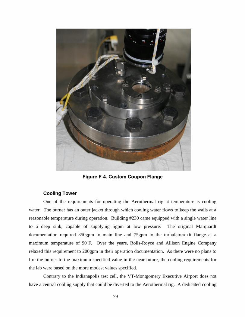
79
Figure F-4. Custom Coupon Flange
Cooling Tower
One of the requirements for operating the Aerothermal rig at temperature is cooling
water. The burner has an outer jacket through which cooling water flows to keep the walls at a
reasonable temperature during operation. Building #230 came equipped with a single water line
to a deep sink, capable of supplying 5gpm at low pressure. The original Marquardt
documentation required 350gpm to main line and 75gpm to the turbulator/exit flange at a
maximum temperature of 90oF. Over the years, Rolls-Royce and Allison Engine Company
relaxed this requirement to 200gpm in their operation documentation. As there were no plans to
fire the burner to the maximum specified value in the near future, the cooling requirements for
the lab were based on the more modest values specified.
Contrary to the Indianapolis test cell, the VT-Montgomery Executive Airport does not
have a central cooling supply that could be diverted to the Aerothermal rig. A dedicated cooling

80
system had to be specified, designed, and installed before the burner could be fired without risk
of mechanical failure. To estimate the heat rejection necessary, the igniter was used to heat up
incoming air, while the cooling jacket was filled with water. The water volume held in the jacket
was measured and the water temperature recorded at multiple points during the test to estimate
an overall heat transfer coefficient.
The igniter was used to heat the mainstream air to 68oC over 30 minutes. The water
temperature rose from 14oC to 39
oC measured in the turbulator. A heat transfer coefficient for
the entire burner jacket based on these calculations was 75W/K during the relatively steady
period 10 minutes after heating started. All water temperature values were averaged over 1
minute intervals to reduce noise in the relatively slow changing values.
Figure F-5. Burner temperatures during HTC test with static water
Extrapolating this data, it was determined that at 1000oC (the maximum value we
intended to fire the burner to in the foreseeable future), approximately 130kW of cooling would
be needed at steady state to keep the water temperature below 90oF. Expecting heat rejection to
increase with convection on the cooling water side when water was flowing and also to give
ourselves an ample factor of safety, a cooling tower was specified and purchased that would
nominally supply 211kW of cooling power. This unit was a T-260 Counterflow Induced Draft
81
Cooling Tower from Cooling Tower Systems in Macon, GA. This unit, pictured in Figure F-6,
would supply sufficient cooling at a range of wet-bulb temperatures from 65-75oF and had a
nominal flow rate of 177gpm. The cooling tower was paired with a self-priming, cast iron
centrifugal pump. The pump has a 316SS impeller capable of handling 3/8” diameter solids and
the 5hp motor can supply 180gpm at 60ft of head.
Figure F-6. Cooling Tower and Rig Exhaust
The cooling tower was installed outside the building on the exhaust side. 4 reinforced
concrete blocks were fabricated to the right height then surrounded with crushed gravel for
additional lateral support. Anti-vibration mats were installed underneath the cooling tower and
the 5hp pump. All of the piping was installed by VT students netting an approximate $5,000
savings over quotes from Physical Plant. The electrical work to supply power to the new
components was completed through Physical plant. A diagram of the additional electrical
components to supply the cooling system is attached below in Figure F-7 below, thanks to Avi
Friedman.
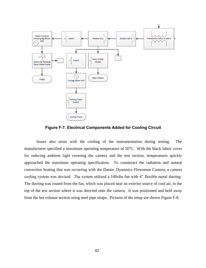
82
Figure F-7. Electrical Components Added for Cooling Circuit
Issues also arose with the cooling of the instrumentation during testing. The
manufacturer specified a maximum operating temperature of 50oC. With the black fabric cover
for reducing ambient light covering the camera and the test section, temperatures quickly
approached the maximum operating specification. To counteract the radiation and natural
convection heating that was occurring with the Dantec Dyanmics Flowsense Camera, a camera
cooling system was devised. The system utilized a 140cfm fan with 4” flexible metal ducting.
The ducting was routed from the fan, which was placed near an exterior source of cool air, to the
top of the test section where it was directed onto the camera. It was positioned and held away
from the hot exhaust section using steel pipe straps. Pictures of the setup are shown Figure F-8.
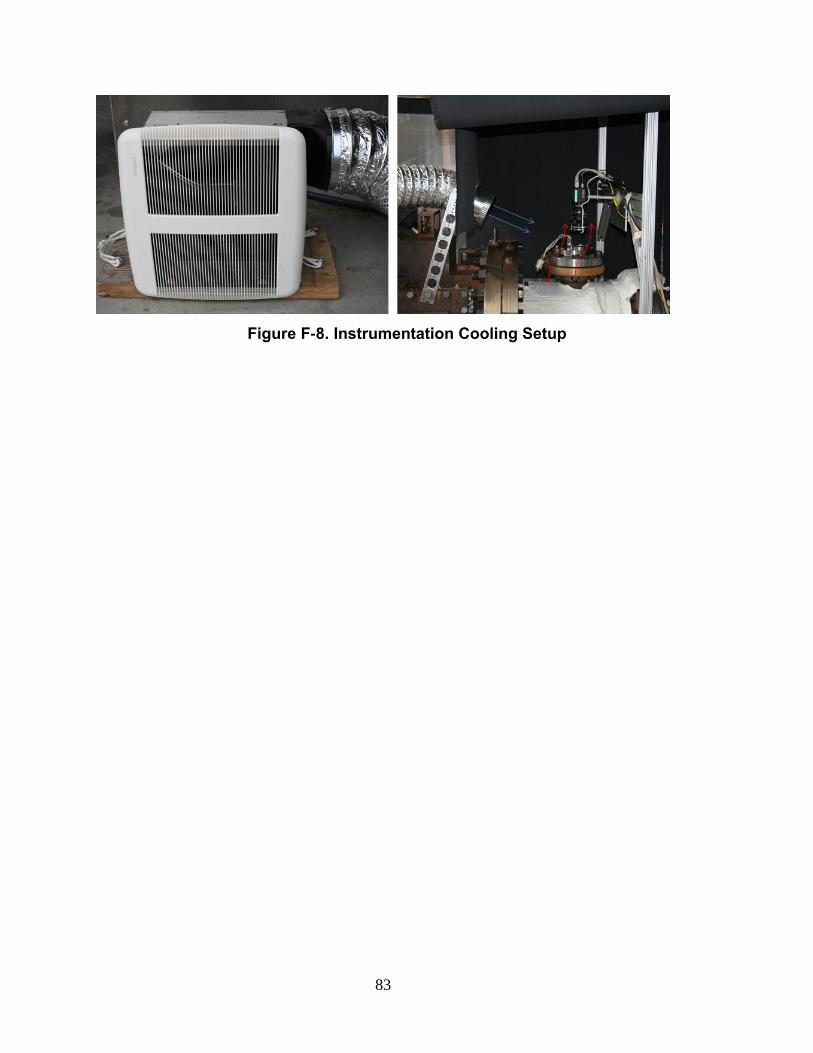
83
Figure F-8. Instrumentation Cooling Setup

84
G. APPENDIX: COR Data Reduction Code
Two parts of the data reduction code are presented in this appendix. The first code, Post
Processing PTV txt files, builds on the open source PTV code by Grier, Crocker and Weeks and
coded for Matlab® by Blair and Dufresne. The open source code tracked individual particles
through a time series of images to output velocity vectors into a txt file. In this study, particles
were only able to be tracked through one image pair. This open source PTV code was slightly
modified to output only vectors with trivial solutions (i.e. one possible vector from frame 1 to
frame b). Particles that had multiple possible vectors from frame 1 to frame 2 could be located
using some additional features in the code but were excluded from this analysis to only keep the
highest fidelity vectors. This open source code is not included here as the contributions by the
author to this piece of code are minor. The original code can be found at
http://physics.georgetown.edu/matlab/
The rationale for including the author’s codes here is the substantial contribution of the
author to the hybrid PTV/CFD technique. The Post processing PTV txt files code, attached
below, takes the output from the tracking code and integrates the CFD output from CFX®. The
code classifies the measured vectors, tracks them forwards or backwards, eliminates erroneous
measurements, and calculates COR for one experiment. The Post Processing Results file
attached in the second subsection takes the results from all of the experiments and calculates the
average incoming parameters for each coupon angle from all experiments; calculates new COR
values for each rebounding particle based on the average incoming parameters; calculates mean
COR values for all particles across all angles and standard deviation for every angle of impact.
While making the measurements are of primary importance to the success of the
technique, without this code, the measured data would be of very little practical importance. The
code is provided here to give the reader additional details and specifics as to how the code was
implemented and the results calculated. It provides a framework for a future researcher looking
to use this technique for their own experiments.
Post Processing PTV txt files
%% Post Processing PTV txt files if exist('rootname') clearvars -except rootname close all else clear all

85
rootname = ''; close all; end
graymon %% Constants
pressAtm = 30.3*3386.389; %inHg -> Pa RAir = 287; %J/kg*K rhoAir = pressAtm/RAir/temp; %kg/m^3 offset = 23.8; %rod center to coupon face mm
temp = 273+27; %K
Davg = 29.25; %um by Volume ARD 20-40um % Davg = 13.46; %um by Volume ARD 10-20 % Davg = 100; %um glass disruptor beads % Davg = 1.020; %um 1% ARD Ultrafine % Davg = 11.54; %um 99% ARD Ultrafine % Davg = 12.49; %um by volume ARD Medium
mass = vol*2650; %kg ARD % mass = vol*2525; %kg glass beads
disp({'Particle Density is ' num2str(mass/vol) ' (ARD = 2650 kg/m^3)' ]) disp(['Mean Particle Diameter is ' num2str(Davg) 'um']) disp(['Current temperature is ' num2str(temp) 'degK'])
radius = Davg/2/1000/1000; %m vol = 4/3*pi*(radius)^3; %m
% Fgrav = mass * 9.81; %N
nuAir =-1.1555*10^(-14)*temp^3+9.5728*10^(-11)*temp^2+3.7604*10^(-8)... *temp-3.4484*10^(-6); % N*s/m^2 @ Temp muAir = nuAir*rhoAir;
qscale = 0.1; %quiver scale for plots
%% Set up fudgeang = 0; % ReTable = dlmread('SmoothSphereDrag.txt', '\t'); % Read Re-Cd table
[file, rootname] = uigetfile([rootname '*.txt'],... 'Please select first results file...'); firstfile = file(strfind(file, '0'):strfind(file, '.')-1); uniqfile = file(1:strfind(file, '0')-1); filenum = str2double(file(strfind(file, '0'):strfind(file, '.')-1)); disp(['Loading from '... rootname(strfind(rootname, 'deg')+4:length(rootname)-1)])
% [ifile, rootname] = uigetfile([rootname,'*.jpg'],... 'Please Select the test image... '); % filename1 = [rootname ifile];
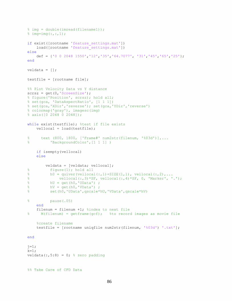
86
% img = double(imread(filename1)); % img=img(:,:,1);
if exist([rootname 'feature_settings.mat']) load([rootname 'feature_settings.mat']) else def = {'0 0 2048 1550','12','35','64.7077', '31','45','65','25'}; end
veldata = [];
testfile = [rootname file];
%% Plot Velocity Data vs Y distance scrsz = get(0,'ScreenSize'); % figure('Position', scrsz); hold all; % set(gca, 'DataAspectRatio', [1 1 1]) % set(gca,'XDir','reverse'); set(gca,'YDir','reverse') % colormap('gray'), imagesc(img) % axis([0 2048 0 2048]);
while exist(testfile); %test if file exists vellocal = load(testfile);
% text (800, 1800, ['Frame#' num2str(filenum, '%03d')],... % 'BackgroundColor',[1 1 1] )
if isempty(vellocal) else
veldata = [veldata; vellocal]; % figure(1); hold all % h0 = quiver(vellocal(:,1)+SIZE(1,1), vellocal(:,2),... % vellocal(:,3)*SF, vellocal(:,4)*SF, 0, 'Marker', '.'); % hU = get(h0,'UData') ; % hV = get(h0,'VData') ; % set(h0,'UData',qscale*hU,'VData',qscale*hV)
% pause(.05) end filenum = filenum +1; %index to next file % M(filenum) = getframe(gcf); %to record images as movie file
%create filename testfile = [rootname uniqfile num2str(filenum, '%03d') '.txt'];
end
j=1; k=1; veldata(:,5:8) = 0; % zero padding
%% Take Care of CFD Data

87
rootnameCFD = rootname(1:strfind(rootname, 'deg')+3); CFDscale = 10000; %m to # of cells
if exist([rootnameCFD 'CFDimported.mat']) load ([rootnameCFD 'CFDimported.mat']) disp('CFD loaded') else [file, rootnameCFD] = uigetfile([rootnameCFD '*.txt'],... 'Please select CFD file...'); CFD = csvread([rootnameCFD file]); % CFD = sort(CFD, 1);
X = CFDscale*CFD(:,1); Z = CFDscale*CFD(:,3); Xmax = round(max(X)); %mm Zmax = round(max(Z)); %mm Xmin = round(min(X)); %mm Zmin = round(min(Z)); %mm
Xi = (Xmin:Xmax); Zi = (Zmin:Zmax)';
U = zeros(length(Xi), length(Zi)); W = U;
for i = 1:length(X) U(round(X(i))+1-Xmin, round(Z(i))+1-Zmin) = CFD(i,4); W(round(X(i))+1-Xmin, round(Z(i))+1-Zmin) = CFD(i,6); end
FU = TriScatteredInterp(CFD(:,1), CFD(:,3), CFD(:,4)); FV = TriScatteredInterp(CFD(:,1), CFD(:,3), CFD(:,6)); [Zg, Xg] = meshgrid(Zi, Xi);
%check un-interpolated plots [r c] = size(U); bar = waitbar(0, 'Filling Scattered Grids...'); for i = 1:length(Xi) for k = 1:length(Zi) if(U(i,k) == 0) U(i,k) = FU(Xg(i,k)/CFDscale, Zg(i,k)/CFDscale); W(i,k) = FV(Xg(i,k)/CFDscale, Zg(i,k)/CFDscale); end end bar = waitbar(i/length(Xi)); end close(bar)
save([rootnameCFD 'CFDimported'], 'U', 'W', 'X','Z', 'Xi', 'Zi', ... 'Xg', 'Zg', 'Xmax', 'Xmin', 'Zmax', 'Zmin')
end
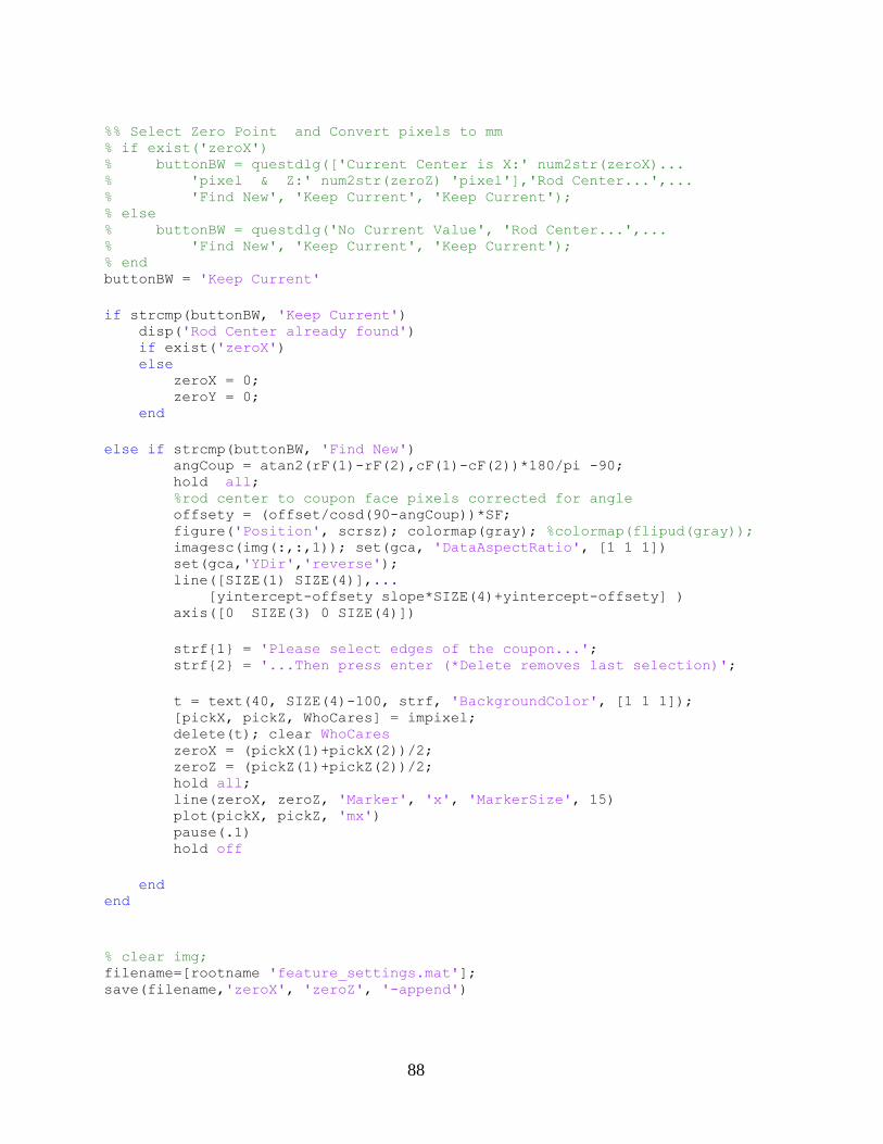
88
%% Select Zero Point and Convert pixels to mm % if exist('zeroX') % buttonBW = questdlg(['Current Center is X:' num2str(zeroX)... % 'pixel & Z:' num2str(zeroZ) 'pixel'],'Rod Center...',... % 'Find New', 'Keep Current', 'Keep Current'); % else % buttonBW = questdlg('No Current Value', 'Rod Center...',... % 'Find New', 'Keep Current', 'Keep Current'); % end buttonBW = 'Keep Current'
if strcmp(buttonBW, 'Keep Current') disp('Rod Center already found') if exist('zeroX') else zeroX = 0; zeroY = 0; end
else if strcmp(buttonBW, 'Find New') angCoup = atan2(rF(1)-rF(2),cF(1)-cF(2))*180/pi -90; hold all; %rod center to coupon face pixels corrected for angle offsety = (offset/cosd(90-angCoup))*SF; figure('Position', scrsz); colormap(gray); %colormap(flipud(gray)); imagesc(img(:,:,1)); set(gca, 'DataAspectRatio', [1 1 1]) set(gca,'YDir','reverse'); line([SIZE(1) SIZE(4)],... [yintercept-offsety slope*SIZE(4)+yintercept-offsety] ) axis([0 SIZE(3) 0 SIZE(4)])
strf{1} = 'Please select edges of the coupon...'; strf{2} = '...Then press enter (*Delete removes last selection)';
t = text(40, SIZE(4)-100, strf, 'BackgroundColor', [1 1 1]); [pickX, pickZ, WhoCares] = impixel; delete(t); clear WhoCares zeroX = (pickX(1)+pickX(2))/2; zeroZ = (pickZ(1)+pickZ(2))/2; hold all; line(zeroX, zeroZ, 'Marker', 'x', 'MarkerSize', 15) plot(pickX, pickZ, 'mx') pause(.1) hold off
end end
% clear img; filename=[rootname 'feature_settings.mat']; save(filename,'zeroX', 'zeroZ', '-append')
89
% zero pixels veldata(:,1) = veldata(:,1) - zeroX; veldata(:,2) = veldata(:,2) - zeroZ; %scale from mm to pixel
veldata(:,1) = veldata(:,1)/SF; veldata(:,2) = veldata(:,2)/SF; veldata(:,:) = -veldata(:,:);
%coupon edge in mm rFmm = (zeroZ - rF(1:2))/SF; cFmm = (zeroX - cF(1:2))/SF;
angCoup = atan2(rFmm(2)-rFmm(1),cFmm(2)-cFmm(1))*180/pi +180; disp(['Angle of the Coupon is ' num2str(90-angCoup)])
%% Rotate Angle figure('Position', scrsz); hold all; axis([-30 60 -70 20]) set(gca, 'DataAspectRatio', [1 1 1], 'FontSize', 20) quiver(veldata(:,1), veldata(:,2),veldata(:,3), veldata(:,4), 2,'r') plot([cFmm; cFmm(1)], [rFmm; rFmm(1)], 'k', 'Marker', 'h') xlabel('X position (mm)');ylabel('Z position (mm)'); legend('Rebound', 'Incoming');
degree = str2num(rootname(strfind(rootname, 'deg')-2:... strfind(rootname, 'deg')-1)); degreeCoup = 90-angCoup; delta = 360 + degreeCoup - degree;
veldata(:,3) = veldata(:,3).*cosd(delta) - veldata(:,4).*sind(delta); veldata(:,4) = veldata(:,3).*sind(delta) + veldata(:,4).*cosd(delta); cFmm = cFmm.*cosd(delta) - rFmm.*sind(delta); rFmm = cFmm.*sind(delta) + rFmm.*cosd(delta);
quiver(veldata(:,1), veldata(:,2),veldata(:,3), veldata(:,4), 2)
slopemm = (rFmm(1)-rFmm(2))/(cFmm(1)-cFmm(2)); yinterceptmm = rFmm(1)-slopemm*cFmm(1); slopeInv = -1/slopemm;
rFmm(3) = rFmm(2)+((19^2)/(1+(1/slopeInv^2)))^.5; cFmm(3) = cFmm(2)+(rFmm(3)-rFmm(2))/(slopeInv); rFmm(4) = rFmm(1)+((19^2)/(1+(1/slopeInv^2)))^.5; cFmm(4) = cFmm(1)+(rFmm(4)-rFmm(1))/(slopeInv); plot([cFmm; cFmm(1)], [rFmm; rFmm(1)], 'b', 'Marker', 'h')
hold off %% Identify Rebounding Particles angCoup = atan2(rFmm(2)-rFmm(1),cFmm(2)-cFmm(1))*180/pi +180; disp(['Angle of the Coupon is ' num2str(90-angCoup)]) angParticle = atan2(veldata(:,4), veldata(:,3))*180/pi;

90
rebound = zeros(size(veldata)); % fudge = zeros(size(veldata));l=1; incoming = zeros(size(veldata));
n=1; m=1; for i = 1:length(veldata) if(angParticle(i)<0) angParticle(i) = angParticle(i)+360; end
if((angParticle(i)-angCoup) < 0 || angParticle(i) > 180 + angCoup) rebound(n,:) = veldata(i,:); n=n+1; % else if ((angParticle(i)-angCoup) > -fudgeang &&... % (angParticle(i)-angCoup) <= 0) % fudge(l,:) = veldata(i,:); % l = l+1; else incoming(m,:) = veldata(i,:); m=m+1; % end end end
rebound(n:size(rebound,1),:) = []; % fudge(l:length(fudge),:) = []; incoming(m:size(incoming,1),:) = [];
rebound = sortrows(rebound); rebound(:,9:10) = 0; % fudge = sortrows(fudge); incoming = sortrows(incoming); incoming(:,9:10) = 0; rejected = []; %maximum measured velocity, calculated can not exceed maxIn = max(hypot(incoming(:,3), incoming(:,4)))
%% Track Backwards for Rebound Velocity Xmaxmm = Xmax*1000/CFDscale; %CFD domain size in mm Xminmm = Xmin*1000/CFDscale; Zmaxmm = Zmax*1000/CFDscale; Zminmm =Zmin*1000/CFDscale;
rejected_Hist = zeros(1,10,1); rebTrack_Hist = zeros(50,size(rebound,2), size(rebound,1));
i=1; bar = waitbar(0, 'Tracking Backwards...'); while i <= size(rebound,1) Track = rebound(i,:) ; n = 1; while(Track(2)<(slopemm*Track(1)+yinterceptmm) ... && Track(1)<Xmaxmm && Track(1)>Xminmm ... && Track(2)>Zminmm && Track(2)< Zmaxmm)

91
%index # for CFD domain xpos = round(Track(1)*CFDscale/1000+1-Xmin); zpos = round(Track(2)*CFDscale/1000+1-Zmin);
%calculate drag %delta U, delta V uCFD = U(xpos,zpos); wCFD = W(xpos,zpos);
delU = Track(3) - uCFD; delW = Track(4) - wCFD;
ReU = abs(delU*2*radius/nuAir); ReW = abs(delW*2*radius/nuAir);
%drag force always positive, velocity not so much Cd = (24.0/ReU)+((2.6*ReU/5.0)/(1+(ReU/5.0)^1.52))+... ((0.411*(ReU/263000)^-7.94)/(1+(ReU/263000)^-8.00))+... (ReU^0.80/461000); FdragU = Cd*0.5*rhoAir*delU*abs(delU)*(pi*(radius)^2);
Cd = (24.0/ReW)+((2.6*ReW/5.0)/(1+(ReW/5.0)^1.52))+... ((0.411*(ReW/263000)^-7.94)/(1+(ReW/263000)^-8.00))+... (ReW^0.80/461000); FdragW = Cd*0.5*rhoAir*(delW*abs(delW))*(pi*(radius)^2);
%find old position/velocity t = time/10^6;
if n==1 perpDist = abs(Track(2)-... slopemm*Track(1)-yinterceptmm)/sqrt(1+slope^2); end
Track(5) = Track(3) + FdragU/mass*(t); Track(6) = Track(4) + FdragW/mass*(t); Track(7) = FdragU; Track(8) = FdragW;
Track(1) = Track(1) - Track(5)*1000*t; Track(2) = Track(2) - Track(6)*1000*t;
rebTrack_Hist(n,:,i) = Track(:); %set for next iteration Track(3) = Track(5); Track(4) = Track(6); n=n+1; end
rebound(i,5) = Track(1); % new x position rebound(i,6) = Track(2); % new y position

92
rebound(i,7) = Track(3); % new u velocity rebound(i,8) = Track(4); % new z velocity if(exist('perpDist')) rebound(i,9) = perpDist; else rebound(i,9) = 0; end rebound(i,10) = n;
if (Track(1)>cFmm(1) || Track(1)<cFmm(2) ||... hypot(Track(3),Track(4))>maxIn || isnan(Track(4))) rejected = [rejected ; rebound(i,:)]; if(size(rejected_Hist,1)< size(rebTrack_Hist,1)) rejected_Hist(size(rejected_Hist,1)+1:... size(rebTrack_Hist,1),:,:) = 0; end rejected_Hist = cat(3, rejected_Hist ,rebTrack_Hist(:,:,i)); rebound(i,:) = []; rebTrack_Hist(:,:,i) = []; else i = i+1; end
bar = waitbar(i/size(rebound,1)); end close(bar)
rejected_Hist(:,:,1) = [];
%% Track Forwards for Incoming Velocity
inTrack_Hist = zeros(100,size(incoming,2), size(incoming,1)); m = size(rejected,1)+1; ww = zeros(size(incoming, 1),1); disp(['There are ' num2str(size(incoming, 1)) ' incoming particles']) rejected_Hist = cat(3, rejected_Hist, zeros(size(rejected_Hist, 1),... size(rejected_Hist, 2), size(incoming, 1))); rejected = [rejected; zeros(size(incoming,1), 10)];
i=1; bar = waitbar(0, 'Tracking Forwards...'); while i <= size(incoming,1) Track = incoming(i,:); n = 1; while(Track(2)<(slopemm*Track(1)+yinterceptmm) ... && Track(1)<Xmaxmm-20 && Track(1)>Xminmm+20 ... && Track(2)<Zmaxmm && Track(2)>Zminmm)
xpos = round(Track(1)*CFDscale/1000+1-Xmin); zpos = round(Track(2)*CFDscale/1000+1-Zmin);
%calculate drag %delta U, delta V uCFD = U(xpos,zpos); wCFD = W(xpos,zpos);

93
delU = uCFD - Track(3); delW = wCFD - Track(4);
ReU = abs(delU*2*radius/nuAir); ReW = abs(delW*2*radius/nuAir);
%drag force always positive, velocity not so much %drag force always positive? velocity not so much Cd = (24.0/ReU)+((2.6*ReU/5.0)/(1+(ReU/5.0)^1.52))+... ((0.411*(ReU/263000)^-7.94)/(1+(ReU/263000)^-8.00))+... (ReU^0.80/461000); FdragU = Cd*0.5*rhoAir*delU*abs(delU)*(pi*(radius)^2);
Cd = (24.0/ReW)+((2.6*ReW/5.0)/(1+(ReW/5.0)^1.52))+... ((0.411*(ReW/263000)^-7.94)/(1+(ReW/263000)^-8.00))+... (ReW^0.80/461000); FdragW = Cd*0.5*rhoAir*(delW*abs(delW))*(pi*(radius)^2);
%find old position/velocity t = time/10^6; if n == 1 perpDist = abs(Track(2)-... slopemm*Track(1)-yinterceptmm)/sqrt(1+slope^2); end
Track(5) = Track(3) + FdragU/mass*(t); Track(6) = Track(4) + FdragW/mass*(t);
Track(1) = Track(1) + Track(5)*1000*t; Track(2) = Track(2) + Track(6)*1000*t; Track(7) = FdragU; Track(8) = FdragW;
%track history inTrack_Hist(n,:,i) = Track(:); %set for next iteration Track(3) = Track(5); Track(4) = Track(6); n=n+1; end
incoming(i,5) = Track(1); incoming(i,6) = Track(2); incoming(i,7) = Track(3); incoming(i,8) = Track(4); incoming(i,9) = perpDist; incoming(i,10) = n;
if (Track(1)>cFmm(1) || Track(1)<cFmm(2) || isinf(Track(4)) ||... hypot(Track(3),Track(4))>maxIn || isnan(Track(4))) rejected(m,:) = incoming(i,:);

94
if(size(rejected_Hist,1)< size(inTrack_Hist,1)) rejected_Hist(size(rejected_Hist,1)+1:... size(inTrack_Hist,1),:,:) = 0; end if(size(rejected_Hist,1)> size(inTrack_Hist,1)) inTrack_Hist(size(inTrack_Hist,1)+1:... size(rejected_Hist,1),:,:) = 0; end
rejected_Hist(:,:,m) = inTrack_Hist(:,:,i); m = m+1; ww(i) = i; i = i+1; else i = i+1; end
bar = waitbar(i/size(incoming,1)); end close(bar)
incoming(find(ww), :) = []; inTrack_Hist(:,:,find(ww)) = []; rejected(m:size(rejected,1),:) = []; rejected_Hist(:,:,m:size(rejected_Hist,3)) = []; %procedural
%% Double Bounce Incoming oneb = zeros(size(incoming,1),1); one = 0; twob = zeros(size(incoming,1), 1); two = 0;
trans = maxIn/2; %m/s
for i = 1:length(incoming) if hypot(incoming(i,7), incoming(i,8))>trans one = one+1; oneb(one) = i; else two = two+1; twob(two,:) = i; end end
oneb(one+1:length(oneb)) = []; twob(two+1:length(twob)) = [];
vv = zeros(size(incoming,1), 1); i=1; bar = waitbar(0, 'Tracking Backwards for Incoming double bounce...'); while i <= size(twob,1) Track = incoming(twob(i),:) ; n = 1; cond = 1; while(cond)

95
%index # for CFD domain xpos = round(Track(1)*CFDscale/1000+1-Xmin); zpos = round(Track(2)*CFDscale/1000+1-Zmin);
%calculate drag %delta U, delta V uCFD = U(xpos,zpos); wCFD = W(xpos,zpos);
delU = Track(3) - uCFD; delW = Track(4) - wCFD;
ReU = abs(delU*2*radius/nuAir); ReW = abs(delW*2*radius/nuAir);
%drag force always positive, velocity not so much Cd = (24.0/ReU)+((2.6*ReU/5.0)/(1+(ReU/5.0)^1.52))+... ((0.411*(ReU/263000)^-7.94)/(1+(ReU/263000)^-8.00))+... (ReU^0.80/461000); FdragU = Cd*0.5*rhoAir*delU*abs(delU)*(pi*(radius)^2);
Cd = (24.0/ReW)+((2.6*ReW/5.0)/(1+(ReW/5.0)^1.52))+... ((0.411*(ReW/263000)^-7.94)/(1+(ReW/263000)^-8.00))+... (ReW^0.80/461000); FdragW = Cd*0.5*rhoAir*(delW*abs(delW))*(pi*(radius)^2);
%find old position/velocity t = time/10^6;
if n==1 perpDist = abs(Track(2)-... slopemm*Track(1)-yinterceptmm)/sqrt(1+slope^2); end
Track(5) = Track(3) + FdragU/mass*(t); Track(6) = Track(4) + FdragW/mass*(t); Track(7) = FdragU; Track(8) = FdragW;
Track(1) = Track(1) - Track(5)*1000*t; Track(2) = Track(2) - Track(6)*1000*t;
twoBTrack_Hist(n,:,i) = Track(:); %set for next iteration Track(3) = Track(5); Track(4) = Track(6); n=n+1;
cond = Track(2)<(slopemm*Track(1)+yinterceptmm) ... && Track(1)<60 && Track(1)>-30 && Track(2)>-70 && Track(2)< 0; end
96
if (Track(1)<cFmm(1) && Track(1)>cFmm(2) && Track(2)>-70) rejected(m,:) = incoming(twob(i),:); rejected(m,10) = 2222; m = m+1; vv(twob(i)) = twob(i); i = i+1; else twoBTrack_Hist(:,:,i) = []; i = i+1; end
bar = waitbar(i/size(twob,1)); end close(bar)
% Plot by Location % measurement history figure('Position', scrsz); hold all; axis([-30 60 -70 20]) set(gca, 'DataAspectRatio', [1 1 1], 'FontSize', 20) h1 = quiver(incoming(:,1), incoming(:,2),... incoming(:,3), incoming(:,4), 0,'r'); h2 = quiver(incoming(twob,1), incoming(twob,2),... incoming(twob,3), incoming(twob,4), 0,'g'); h3 = quiver(incoming(find(vv),1), incoming(find(vv),2),... incoming(find(vv),3), incoming(find(vv),4), 0,'b'); hU = get(h1,'UData') ; hV = get(h1,'VData') ; set(h1,'UData',qscale*hU,'VData',qscale*hV) hU = get(h2,'UData') ; hV = get(h2,'VData') ; set(h2,'UData',qscale*hU,'VData',qscale*hV) hU = get(h3,'UData') ; hV = get(h3,'VData') ; set(h3,'UData',qscale*hU,'VData',qscale*hV) plot([cFmm; cFmm(1)], [rFmm; rFmm(1)], 'k', 'Marker', 'h') xlabel('X position (mm)');ylabel('Z position (mm)'); legend('One Bounce', 'Two Bounce Suspects', 'Two Bounce Confirmed'); hold off
%track history successful if (exist('twoBTrack_Hist')) figure('Position', scrsz); hold all; set(gca, 'XDir', 'reverse') axis([-30 50 -70 0]) set(gca, 'DataAspectRatio', [1 1 1], 'FontSize', 20) quiver(inTrack_Hist(:,1,find(vv)), inTrack_Hist(:,2,find(vv)),... inTrack_Hist(:,3,find(vv)), inTrack_Hist(:,4,find(vv)), 3,'r') quiver(twoBTrack_Hist(:,1,:), twoBTrack_Hist(:,2,:),... twoBTrack_Hist(:,3,:), twoBTrack_Hist(:,4,:), 3,'m') fill(cFmm, rFmm, 'k', 'Marker', 'h')
xlabel('X position (mm)');ylabel('Z position (mm)'); legend('Incoming History', 'Double Bounce', 'Location', 'Best'); hold off end

97
[n_in, x] = hist(hypot(incoming(:,7), incoming(:,8)), 1:1:round(maxIn)); incoming(find(vv), :) = []; [ndb_in,x] = hist(hypot(incoming(:,7), incoming(:,8)), 1:1:round(maxIn)); inTrack_Hist(:,:,find(vv)) = [];
[ndb_reb,x] = hist(hypot(rebound(:,7), rebound(:,8)), 1:1:round(maxIn));
inCFDcomp = zeros(size(incoming,1), 1); for i = 1:size(incoming,1) xpos = round(incoming(i,1)*CFDscale/1000)+1-Xmin; zpos = round(incoming(i,2)*CFDscale/1000)+1-Zmin; inCFDcomp(i,1:2) = [incoming(i,1) incoming(i,2)]; inCFDcomp(i,3:4) = [U(xpos,zpos) W(xpos, zpos)];
end inCFDcomp(:,5:6) = [(incoming(:,3)-inCFDcomp(:,3))... (incoming(:,4) - inCFDcomp(:,4))]; inCFDcomp(:,7:8) = [(incoming(:,3)-inCFDcomp(:,3))./... inCFDcomp(:,3) (incoming(:,4) - inCFDcomp(:,4))./inCFDcomp(:,4)];
rejected_CFD = []; % filter incoming particles i = 1; while i <= size(incoming,1) if ((abs(inCFDcomp(i,5))>10 && abs(inCFDcomp(i,7))>2) ||... (abs(inCFDcomp(i,5))> 2 && abs(inCFDcomp(i,7))> 10)) rejected_CFD = [rejected_CFD; incoming(i,:)]; incoming(i,:) = []; inCFDcomp(i,:) = []; inTrack_Hist(:,:,i) = []; else i = i+1; end end
%% calc values along edge/last track rebEdge = zeros(size(rebound,1), 4); rebEdge(:,1:2) = rebound(:,5:6); rebEdge(:,3) = hypot(rebound(:,7), rebound(:,8)); rebEdge(:,4) = atan2(rebound(:,8), rebound(:,7))*180/pi;
% for i = 1:length(rebEdge) % if(rebEdge(i,4)> 0) % rebEdge(i,4)=rebEdge(i,4)-angCoup; % else % rebEdge(i,4)=360+rebEdge(i,4) - angCoup; % end % if rebEdge(i,4)>90 % rebEdge(i,4) = abs(rebEdge(i,4)-180); % end % end
inEdge = zeros(size(incoming,1), 4);

98
inEdge(:,1:2) = incoming(:,5:6); inEdge(:,3) = hypot(incoming(:,7), incoming(:,8)); inEdge(:,4) = atan2(incoming(:,8), incoming(:,7))*180/pi; for i = 1:length(inEdge) if(inEdge(i,4)> 0) inEdge(i,4)=inEdge(i,4)-angCoup; else inEdge(i,4)=360+inEdge(i,4) -angCoup; end if(inEdge(i,4)> 90) inEdge(i,4)=abs(inEdge(i,4)-180); end end
rebEdge = sortrows(rebEdge, 1); inEdge = sortrows(inEdge, 1);
smoothF = 20; smoothrebEdge = rebEdge; smoothinEdge = inEdge; % smoothrebEdge(:,3) = smooth(rebEdge(:,3),... % round(size(rebound,1)/smoothF), 'rlowess'); %comment out for raw smoothinEdge(:,3) = smooth(inEdge(:,3),... round(size(incoming,1)/smoothF), 'rlowess'); % smoothrebEdge(:,4) = smooth(rebEdge(:,4),... % round(size(rebound,1)/smoothF), 'rlowess'); %comment out for raw smoothinEdge(:,4) = smooth(inEdge(:,4),... round(size(incoming,1)/smoothF), 'rlowess');
cutF = 12; smoothrebEdge = smoothrebEdge(round(size(rebound,1)/cutF):... length(rebound)- round(size(rebound,1)/cutF), :); smoothreb = rebound(round(size(rebound,1)/cutF):... length(rebound)- round(size(rebound,1)/cutF), :); % smoothinEdge = smoothinEdge(round(size(incoming,1)/smoothF):... % length(incoming)- round(size(incoming,1)/smoothF), :);
%% COR smoothinEdgeInterp(:,1:2) = smoothrebEdge(:,1:2); [d, e] = unique(smoothinEdge(:,1)); %removes repeat x values, error interp1 smoothinEdge = smoothinEdge(e,:); smoothinEdgeInterp (:,3) = interp1(smoothinEdge(:,1),... smoothinEdge(:,3), smoothinEdgeInterp(:,1)); smoothinEdgeInterp (:,4) = interp1(smoothinEdge(:,1),... smoothinEdge(:,4), smoothinEdgeInterp(:,1));
CORang = smoothinEdgeInterp(:,4); CORmag = smoothrebEdge(:,3)./smoothinEdgeInterp(:,3) ;
%% Plot Tracks, Other Stuff, Save figure; plot( x, ndb_reb, '.-', x,n_in, '*-', x, ndb_in, '<-') set(gca, 'FontSize', 20) xlabel('Velocity (m/s'); ylabel ('Count #') legend('Rebound Original', 'Incoming Original',...
99
'Incoming Corrected', 'Location', 'Best')
%track history successful figure('Position', scrsz); hold all; axis([-30 60 -70 20]) set(gca, 'XDir', 'reverse', 'DataAspectRatio', [1 1 1], 'FontSize', 20)
%plot individual tracks % quiver(inTrack_Hist(:,1,numin), inTrack_Hist(:,2,numin),... % inTrack_Hist(:,3,numin), inTrack_Hist(:,4,numin), 1) % quiver(rebTrack_Hist(:,1,numout), rebTrack_Hist(:,2,numout),... % rebTrack_Hist(:,3,numout), rebTrack_Hist(:,4,numout), 1)
quiver(inTrack_Hist(:,1,:), inTrack_Hist(:,2,:),... inTrack_Hist(:,3,:), inTrack_Hist(:,4,:), 3,'r') quiver(rebTrack_Hist(:,1,:), rebTrack_Hist(:,2,:),... rebTrack_Hist(:,3,:), rebTrack_Hist(:,4,:), 3, 'b') fill(cFmm, rFmm, 'k') xlabel('X position (mm)');ylabel('Z position (mm)'); legend('Incoming', 'Coupon', 'Rebound', 'Location', 'SouthWest'); hold off
% %track history rejected % figure('Position', scrsz); hold all; % axis([-30 60 -70 20]) % set(gca, 'DataAspectRatio', [1 1 1], 'FontSize', 20) % quiver(rejected_Hist(:,1,:), rejected_Hist(:,2,:),... % rejected_Hist(:,3,:), rejected_Hist(:,4,:), 5) % plot([cFmm; cFmm(1)], [rFmm; rFmm(1)], 'k', 'Marker', 'h') % xlabel('X position (mm)');ylabel('Z position (mm)'); % hold off
%measurement history figure('Position', scrsz); hold all; axis([-30 60 -70 20]) set(gca, 'DataAspectRatio', [1 1 1], 'FontSize', 20) % quiver(incoming(:,1), incoming(:,2),incoming(:,3), incoming(:,4), 2, 'r') % quiver(rebound(:,1), rebound(:,2),rebound(:,3), rebound(:,4), 2, 'b') fill(cFmm, rFmm, 'k') quiver(incoming(:,1), incoming(:,2),incoming(:,3), incoming(:,4), 2) quiver(rebound(:,1), rebound(:,2),rebound(:,3), rebound(:,4), 2, 'k') % quiver(fudge(:,1), fudge(:,2), fudge(:,3), fudge(:,4), 2,'g') plot([cFmm; cFmm(1)], [rFmm; rFmm(1)], 'k', 'Marker', 'h') xlabel('X position (mm)');ylabel('Z position (mm)'); legend('Coupon', 'Incoming', 'Rebound' ); hold off
cFillmm = [-100 100 100 -100]; rFillmm = [slopemm*cFillmm(1)+yinterceptmm ... slopemm*cFillmm(2)+yinterceptmm 50 50];
Xg = Xg*1000/CFDscale; Zg = Zg*1000/CFDscale;
100
% cfd vs measurements U % figure('Position', scrsz); hold all; % axis([-30 60 -70 20]) % set(gca, 'XDir', 'reverse', 'DataAspectRatio', [1 1 1], 'FontSize', 20) % title('Tracked Particles vs U Velocity (CFD)') % xlabel('X Position (mm)') % ylabel('Z Position (mm)') % contourf(Xg, Zg, U, -30:2:30); colormap gray;... % caxis([-30 30]); colorbar('FontSize', 20); % fill(cFillmm, rFillmm, 'w') % fill(cFmm, rFmm, 'k') % plot([cFmm; cFmm(1)], [rFmm; rFmm(1)], 'k', 'Marker', 'h') % quiver(incoming(:,1), incoming(:,2), incoming(:,3), incoming(:,4),'k'); % % quiver(rebound(:,1), rebound(:,2), rebound(:,3), rebound(:,4),'w'); % hold off
% cfd vs measurements W % figure('Position', scrsz); hold all % axis([-30 60 -70 20]) % set(gca, 'XDir', 'reverse', 'DataAspectRatio', [1 1 1], 'FontSize', 20) % title('Tracked Particles vs W Velocity (CFD)') % xlabel('X Position (mm)') % ylabel('Z Position (mm)') % contourf(Xg, Zg, W, -10:2:30); colormap gray;... % caxis([-10 30]); colorbar('FontSize', 20); % % contourf(Xg, Zg, W, -15:2:40); colormap gray; colorbar; % fill(cFillmm, rFillmm, 'w') % fill(cFmm, rFmm, 'k') % plot([cFmm; cFmm(1)], [rFmm; rFmm(1)], 'k', 'Marker', 'h') % % quiver(incoming(:,1), incoming(:,2), incoming(:,3), incoming(:,4),'k'); % % quiver(rebound(:,1), rebound(:,2), rebound(:,3), rebound(:,4), 'w'); % % quiver(incoming(:,1), incoming(:,2), incoming(:,3), incoming(:,4)); % quiver(rebound(:,1), rebound(:,2), rebound(:,3), rebound(:,4),'k'); % hold off
% %measurement vs distance away from plate % figure; hold all; % % set(gca, 'DataAspectRatio', [1 1 1], 'FontSize', 20) % plot( hypot(rebound(:,3), rebound(:,4)), rebound(:,2),'b.') % plot(hypot(incoming(:,3), incoming(:,4)),incoming(:,2),'r.') % plot( hypot(rebound(:,7), rebound(:,8)), rebound(:,2),'c.') % plot(hypot(incoming(:,7), incoming(:,8)),incoming(:,2),'m.') % xlabel('velocity');ylabel('Z position (mm)'); % title('Velocity Magnitude versus Distance from Plate') % legend('Rebound', 'Incoming', 'Calc Rebound',... % 'Calc Incoming', 'Location', 'Best'); % hold off
%plot edge data figure; hold all; % axis([-40 30 0 200]) axis([-30 60 0 90]) set(gca, 'DataAspectRatio', [1 1 1], 'FontSize', 20) plot(rebEdge(:,1),rebEdge(:,3), 'b.') plot(rebEdge(:,1), rebEdge(:,4), 'c.')
101
plot(inEdge(:,1),inEdge(:,3), 'r.') plot(inEdge(:,1), inEdge(:,4), 'm.') plot(smoothrebEdge(:,1), smoothrebEdge(:,3), 'b+') plot(smoothinEdge(:,1), smoothinEdge(:,3), 'r+') plot(smoothrebEdge(:,1), smoothrebEdge(:,4), 'co') plot(smoothinEdge(:,1), smoothinEdge(:,4), 'mo') line([-30 60], [maxIn maxIn], 'LineStyle', ':') plot(smoothinEdgeInterp(:,1), smoothinEdgeInterp(:,4), 'm*') % legend( 'In Mag', 'In Angle',... % 'Avg In Mag', 'Avg In Angle', 'Location', 'NorthWestOutside') legend('Reb Mag', 'Reb Angle', 'In Mag', 'In Angle',... 'Avg Reb Mag', 'Avg In Mag', 'Avg Reb Angle',... 'Avg In Angle', 'Location', 'NorthWestOutside') title('Velocity Magnitude/Angle along the Plate') xlabel('X Position (mm)'); ylabel('Velocity Magnitude(m/s) & Angle (degrees)') hold off
% %plot edge data % figure; hold all; % axis([-30 60 0 90]) % set(gca, 'DataAspectRatio', [1 1 1], 'FontSize', 20) % plot(smoothrebEdge(:,1), smoothrebEdge(:,3), 'b+') % plot(smoothinEdgeInterp(:,1), smoothinEdgeInterp(:,3), 'r+') % plot(smoothinEdgeInterp(:,1), smoothinEdgeInterp(:,4), 'ro') % legend('Rebound Magnitude', 'Average Incoming Mag',... % 'Average Incoming Angle', 'Location', 'Best','FontSize', 20) % line([-30 60], [maxIn maxIn], 'LineStyle', ':') % title('Velocity Magnitude/Angle along the Plate') % xlabel('X Position (mm)'); %ylabel('Velocity Magnitude(m/s) & Angle (degrees)') % hold off
figure; hold all; axis([0 90 0 2]) set(gca, 'FontSize', 20) plot(CORang, CORmag,'.') xlabel('Incoming Angle (degrees)'); ylabel('COR') hold off
filename=[rootname uniqfile 'totals' '.mat']; save(filename,'rebound','incoming', 'smoothrebEdge',... 'smoothinEdge','CORang', 'CORmag')
filename=[rootname 'statistics.mat']; if (exist(filename)) save(filename,'maxIn', 'angCoup', '-append') else save(filename,'maxIn', 'angCoup', '-mat') end

102
Post Processing Results File
%% Post Processing Edge Data close all clc
%% Initialize cstring='rgbmck'; set(0, 'DefaultAxesFontName', 'Arial');
i = 1; filelist = []; CORmag_totals = []; CORang_totals = []; xpos_totals = []; inmag_totals = []; CORmag30deg = []; CORang30deg = []; xpos30deg = []; inmag30deg = [];... smoothrebEdge30deg = []; smoothinEdge30deg = []; rebound30deg = []; CORmag40deg = []; CORang40deg = []; xpos40deg = []; inmag40deg = [];... smoothrebEdge40deg = []; smoothinEdge40deg = []; rebound40deg = []; CORmag50deg = []; CORang50deg = []; xpos50deg = []; inmag50deg = [];... smoothrebEdge50deg = []; smoothinEdge50deg = []; rebound50deg = []; CORmag60deg = []; CORang60deg = []; xpos60deg = []; inmag60deg = [];... smoothrebEdge60deg = []; smoothinEdge60deg = []; rebound60deg = []; CORmag70deg = []; CORang70deg = []; xpos70deg = []; inmag70deg = [];... smoothrebEdge70deg = []; smoothinEdge70deg = []; rebound70deg = []; CORmag80deg = []; CORang80deg = []; xpos80deg = []; inmag80deg = [];... smoothrebEdge80deg = []; smoothinEdge80deg = []; rebound80deg = [];
buttonBW = 'Yes'; root = ''; oldroot = 'init'; scrsz = get(0,'ScreenSize'); %% Load Data count = 0; legen = ''; figure('Position', scrsz); hold all axis([0 90 0 2]); set(gca, 'FontSize', 20) xlabel('Angle of Impact'); ylabel('COR')
while (buttonBW == 'Yes')
[file, root] = uigetfile([root '*CFD.mat'], 'Select the results
file...'); load([root file])
if (strfind(root, oldroot)) disp('Duplicate file name') else count = count+1; %Find naming ... Degrees, Run, Unique degree = root(strfind(root, 'deg')-2:strfind(root, 'deg')+2); run = root(strfind(root, 'un')+2:strfind(root, 'un')+6); disp([degree run file])
%Rename variables and set ang for Fitting

103
filelist = [filelist; [degree '_' run]];
% set up for normal/tan split rebound = sortrows(rebound,5); cutF = 12; rebound = rebound(round(size(rebound,1)/cutF):... length(rebound)- round(size(rebound,1)/cutF), :); smoothrebEdge(:,4) = atan2(rebound(:,8), rebound(:,7))*180/pi;
out = isnan(CORmag); CORmag(out) = []; CORang(out) = []; smoothrebEdge(out,:) = []; rebound(out,:) = [];
eval(['CORang' degree '_' run '= CORang;']); eval(['CORmag' degree '_' run '= CORmag;']); % eval(['incoming' degree '_' run '= incoming;']); % eval(['rebound' degree '_' run '= rebound;']); eval(['smoothinEdge' degree '_' run '= smoothinEdge;']); eval(['smoothrebEdge' degree '_' run '= smoothrebEdge;']); eval(['rebound' degree '_' run '= rebound;']);
xpos = smoothinEdge(:,1); inmag = smoothinEdge(:,3);
eval(['xpos' degree '_' run '= xpos;']); eval(['inmag' degree '_' run '= inmag;']);
eval([['CORmag' degree] '=' ['[CORmag' degree ';' 'CORmag];']]); eval([['CORang' degree] '=' ['[CORang' degree ';' 'CORang];']]); eval([['xpos' degree] '=' ['[xpos' degree ';' 'xpos];']]); eval([['inmag' degree] '=' ['[inmag' degree ';' 'inmag];']]); eval([['smoothrebEdge' degree] '=' ... ['[smoothrebEdge' degree ';' 'smoothrebEdge];']]); eval([['smoothinEdge' degree] '=' ... ['[smoothinEdge' degree ';' 'smoothinEdge];']]); eval([['rebound' degree] '=' ['[rebound' degree ';' 'rebound];']]);
CORmag_totals = [CORmag_totals; CORmag]; CORang_totals = [CORang_totals; CORang]; xpos_totals = [xpos_totals; xpos]; inmag_totals = [inmag_totals; inmag];
legen = [legen; degree '-' run]; oldroot = root; figure(1); plot(CORang, CORmag, 'Line', 'none', 'Marker', 'x',... 'MarkerSize', 5, 'Color', cstring(mod(count,6)+1)) legend(legen, 'Location', 'EastOutside') end
104
buttonBW = questdlg('Input another file?', ' ', 'Yes', 'No ', 'No ');
end hold off
clear CORang CORmag incoming rebound smoothinEdge smoothrebEdge... degree run xpos inmag out
%% Plot CORtan_totals = []; CORnorm_totals = []; CORmag_totals_poly = []; CORang_totals_poly = []; vtan_totals = []; vnorm_totals = [];
if (length(smoothrebEdge30deg) >1) inpoly30deg_coeff = polyfit(xpos30deg, inmag30deg, 6); inpoly30deg_angcoeff = polyfit(smoothrebEdge30deg(:,1), CORang30deg,6);
in_poly30deg = inpoly30deg_coeff(1).*smoothrebEdge30deg(:,1).^6 +... inpoly30deg_coeff(2).*smoothrebEdge30deg(:,1).^5 +... inpoly30deg_coeff(3).*smoothrebEdge30deg(:,1).^4 +... inpoly30deg_coeff(4).*smoothrebEdge30deg(:,1).^3 +... inpoly30deg_coeff(5).*smoothrebEdge30deg(:,1).^2 +... inpoly30deg_coeff(6).*smoothrebEdge30deg(:,1)+inpoly30deg_coeff(7);
ang_poly30deg = inpoly30deg_angcoeff(1).*smoothrebEdge30deg(:,1).^6+... inpoly30deg_angcoeff(2).*smoothrebEdge30deg(:,1).^5 +... inpoly30deg_angcoeff(3).*smoothrebEdge30deg(:,1).^4 +... inpoly30deg_angcoeff(4).*smoothrebEdge30deg(:,1).^3 +... inpoly30deg_angcoeff(5).*smoothrebEdge30deg(:,1).^2 +... inpoly30deg_angcoeff(6).*smoothrebEdge30deg(:,1) +... inpoly30deg_angcoeff(7);
%resolve components angParticle30deg = 90-30-smoothrebEdge30deg(:,4); vtan30deg = cosd(ang_poly30deg).*in_poly30deg; vnorm30deg = sind(ang_poly30deg).*in_poly30deg; Vtan30deg = cosd(angParticle30deg).*smoothrebEdge30deg(:,3); Vnorm30deg = sind(angParticle30deg).*smoothrebEdge30deg(:,3);
COR_tan30deg = Vtan30deg./vtan30deg; COR_norm30deg = Vnorm30deg./vnorm30deg; CORtan_totals = [CORtan_totals; COR_tan30deg]; CORnorm_totals = [CORnorm_totals; COR_norm30deg]; vtan_totals = [vtan_totals; vtan30deg]; vnorm_totals = [vnorm_totals; vnorm30deg];
COR_poly30deg = smoothrebEdge30deg(:,3)./in_poly30deg; CORmag_totals_poly = [CORmag_totals_poly; COR_poly30deg]; CORang_totals_poly = [CORang_totals_poly; ang_poly30deg]; end

105
if (length(smoothrebEdge40deg) >1) inpoly40deg_coeff = polyfit(xpos40deg, inmag40deg, 6); inpoly40deg_angcoeff = polyfit(smoothrebEdge40deg(:,1), CORang40deg,6);
in_poly40deg = inpoly40deg_coeff(1).*smoothrebEdge40deg(:,1).^6+... inpoly40deg_coeff(2).*smoothrebEdge40deg(:,1).^5 +... inpoly40deg_coeff(3).*smoothrebEdge40deg(:,1).^4 +... inpoly40deg_coeff(4).*smoothrebEdge40deg(:,1).^3 +... inpoly40deg_coeff(5).*smoothrebEdge40deg(:,1).^2 +... inpoly40deg_coeff(6).*smoothrebEdge40deg(:,1)+inpoly40deg_coeff(7);
ang_poly40deg = inpoly40deg_angcoeff(1).*smoothrebEdge40deg(:,1).^6+... inpoly40deg_angcoeff(2).*smoothrebEdge40deg(:,1).^5 +... inpoly40deg_angcoeff(3).*smoothrebEdge40deg(:,1).^4 +... inpoly40deg_angcoeff(4).*smoothrebEdge40deg(:,1).^3 +... inpoly40deg_angcoeff(5).*smoothrebEdge40deg(:,1).^2 +... inpoly40deg_angcoeff(6).*smoothrebEdge40deg(:,1) +... inpoly40deg_angcoeff(7);
%resolve components angParticle40deg = 90-40-smoothrebEdge40deg(:,4); vtan40deg = cosd(ang_poly40deg).*in_poly40deg; vnorm40deg = sind(ang_poly40deg).*in_poly40deg; Vtan40deg = cosd(angParticle40deg).*smoothrebEdge40deg(:,3); Vnorm40deg = sind(angParticle40deg).*smoothrebEdge40deg(:,3);
COR_tan40deg = Vtan40deg./vtan40deg; COR_norm40deg = Vnorm40deg./vnorm40deg; CORtan_totals = [CORtan_totals; COR_tan40deg]; CORnorm_totals = [CORnorm_totals; COR_norm40deg]; vtan_totals = [vtan_totals; vtan40deg]; vnorm_totals = [vnorm_totals; vnorm40deg];
COR_poly40deg = smoothrebEdge40deg(:,3)./in_poly40deg; CORmag_totals_poly = [CORmag_totals_poly; COR_poly40deg]; CORang_totals_poly = [CORang_totals_poly; ang_poly40deg]; end
if (length(smoothrebEdge50deg) >1) inpoly50deg_coeff = polyfit(xpos50deg, inmag50deg, 6); inpoly50deg_angcoeff = polyfit(smoothrebEdge50deg(:,1), CORang50deg,6);
in_poly50deg = inpoly50deg_coeff(1).*smoothrebEdge50deg(:,1).^6 +... inpoly50deg_coeff(2).*smoothrebEdge50deg(:,1).^5 +... inpoly50deg_coeff(3).*smoothrebEdge50deg(:,1).^4 +... inpoly50deg_coeff(4).*smoothrebEdge50deg(:,1).^3 +... inpoly50deg_coeff(5).*smoothrebEdge50deg(:,1).^2 +... inpoly50deg_coeff(6).*smoothrebEdge50deg(:,1)+inpoly50deg_coeff(7);
ang_poly50deg = inpoly50deg_angcoeff(1).*smoothrebEdge50deg(:,1).^6+... inpoly50deg_angcoeff(2).*smoothrebEdge50deg(:,1).^5 +... inpoly50deg_angcoeff(3).*smoothrebEdge50deg(:,1).^4 +... inpoly50deg_angcoeff(4).*smoothrebEdge50deg(:,1).^3 +... inpoly50deg_angcoeff(5).*smoothrebEdge50deg(:,1).^2 +... inpoly50deg_angcoeff(6).*smoothrebEdge50deg(:,1) +...

106
inpoly50deg_angcoeff(7);
%resolve components angParticle50deg = 90-50-smoothrebEdge50deg(:,4); vtan50deg = cosd(ang_poly50deg).*in_poly50deg; vnorm50deg = sind(ang_poly50deg).*in_poly50deg; Vtan50deg = cosd(angParticle50deg).*smoothrebEdge50deg(:,3); Vnorm50deg = sind(angParticle50deg).*smoothrebEdge50deg(:,3);
COR_tan50deg = Vtan50deg./vtan50deg; COR_norm50deg = Vnorm50deg./vnorm50deg; CORtan_totals = [CORtan_totals; COR_tan50deg]; CORnorm_totals = [CORnorm_totals; COR_norm50deg]; vtan_totals = [vtan_totals; vtan50deg]; vnorm_totals = [vnorm_totals; vnorm50deg];
COR_poly50deg = smoothrebEdge50deg(:,3)./in_poly50deg; CORmag_totals_poly = [CORmag_totals_poly; COR_poly50deg]; CORang_totals_poly = [CORang_totals_poly; ang_poly50deg]; end
if (length(smoothrebEdge60deg) >1) inpoly60deg_coeff = polyfit(xpos60deg, inmag60deg, 6); inpoly60deg_angcoeff = polyfit(smoothrebEdge60deg(:,1), CORang60deg,6);
in_poly60deg = inpoly60deg_coeff(1).*smoothrebEdge60deg(:,1).^6+... inpoly60deg_coeff(2).*smoothrebEdge60deg(:,1).^5 +... inpoly60deg_coeff(3).*smoothrebEdge60deg(:,1).^4 +... inpoly60deg_coeff(4).*smoothrebEdge60deg(:,1).^3 +... inpoly60deg_coeff(5).*smoothrebEdge60deg(:,1).^2 +... inpoly60deg_coeff(6).*smoothrebEdge60deg(:,1)+inpoly60deg_coeff(7);
ang_poly60deg = inpoly60deg_angcoeff(1).*smoothrebEdge60deg(:,1).^6 +... inpoly60deg_angcoeff(2).*smoothrebEdge60deg(:,1).^5 +... inpoly60deg_angcoeff(3).*smoothrebEdge60deg(:,1).^4 +... inpoly60deg_angcoeff(4).*smoothrebEdge60deg(:,1).^3 +... inpoly60deg_angcoeff(5).*smoothrebEdge60deg(:,1).^2 +... inpoly60deg_angcoeff(6).*smoothrebEdge60deg(:,1) +... inpoly60deg_angcoeff(7);
%resolve components angParticle60deg = 90-60-smoothrebEdge60deg(:,4); vtan60deg = cosd(ang_poly60deg).*in_poly60deg; vnorm60deg = sind(ang_poly60deg).*in_poly60deg; Vtan60deg = cosd(angParticle60deg).*smoothrebEdge60deg(:,3); Vnorm60deg = sind(angParticle60deg).*smoothrebEdge60deg(:,3);
COR_tan60deg = Vtan60deg./vtan60deg; COR_norm60deg = Vnorm60deg./vnorm60deg; CORtan_totals = [CORtan_totals; COR_tan60deg]; CORnorm_totals = [CORnorm_totals; COR_norm60deg]; vtan_totals = [vtan_totals; vtan60deg]; vnorm_totals = [vnorm_totals; vnorm60deg];
COR_poly60deg = smoothrebEdge60deg(:,3)./in_poly60deg;
107
CORmag_totals_poly = [CORmag_totals_poly; COR_poly60deg]; CORang_totals_poly = [CORang_totals_poly; ang_poly60deg]; end
if (length(smoothrebEdge70deg) >1) inpoly70deg_coeff = polyfit(xpos70deg, inmag70deg, 6); inpoly70deg_angcoeff = polyfit(smoothrebEdge70deg(:,1), CORang70deg,6);
in_poly70deg = inpoly70deg_coeff(1).*smoothrebEdge70deg(:,1).^6 +... inpoly70deg_coeff(2).*smoothrebEdge70deg(:,1).^5 +... inpoly70deg_coeff(3).*smoothrebEdge70deg(:,1).^4 +... inpoly70deg_coeff(4).*smoothrebEdge70deg(:,1).^3 +... inpoly70deg_coeff(5).*smoothrebEdge70deg(:,1).^2 +... inpoly70deg_coeff(6).*smoothrebEdge70deg(:,1)+inpoly70deg_coeff(7);
ang_poly70deg = inpoly70deg_angcoeff(1).*smoothrebEdge70deg(:,1).^6+... inpoly70deg_angcoeff(2).*smoothrebEdge70deg(:,1).^5 +... inpoly70deg_angcoeff(3).*smoothrebEdge70deg(:,1).^4 +... inpoly70deg_angcoeff(4).*smoothrebEdge70deg(:,1).^3 +... inpoly70deg_angcoeff(5).*smoothrebEdge70deg(:,1).^2 +... inpoly70deg_angcoeff(6).*smoothrebEdge70deg(:,1) +... inpoly70deg_angcoeff(7);
%resolve components angParticle70deg = 90-70-smoothrebEdge70deg(:,4); vtan70deg = cosd(ang_poly70deg).*in_poly70deg; vnorm70deg = sind(ang_poly70deg).*in_poly70deg; Vtan70deg = cosd(angParticle70deg).*smoothrebEdge70deg(:,3); Vnorm70deg = sind(angParticle70deg).*smoothrebEdge70deg(:,3);
COR_tan70deg = Vtan70deg./vtan70deg; COR_norm70deg = Vnorm70deg./vnorm70deg; CORtan_totals = [CORtan_totals; COR_tan70deg]; CORnorm_totals = [CORnorm_totals; COR_norm70deg]; vtan_totals = [vtan_totals; vtan70deg]; vnorm_totals = [vnorm_totals; vnorm70deg];
COR_poly70deg = smoothrebEdge70deg(:,3)./in_poly70deg; CORmag_totals_poly = [CORmag_totals_poly; COR_poly70deg]; CORang_totals_poly = [CORang_totals_poly; ang_poly70deg]; end
if (length(smoothrebEdge80deg) >1) inpoly80deg_coeff = polyfit(xpos80deg, inmag80deg, 6); inpoly80deg_angcoeff = polyfit(smoothrebEdge80deg(:,1), CORang80deg,6);
in_poly80deg = inpoly80deg_coeff(1).*smoothrebEdge80deg(:,1).^6 +... inpoly80deg_coeff(2).*smoothrebEdge80deg(:,1).^5 +... inpoly80deg_coeff(3).*smoothrebEdge80deg(:,1).^4 +... inpoly80deg_coeff(4).*smoothrebEdge80deg(:,1).^3 +... inpoly80deg_coeff(5).*smoothrebEdge80deg(:,1).^2 +... inpoly80deg_coeff(6).*smoothrebEdge80deg(:,1)+inpoly80deg_coeff(7);
ang_poly80deg = inpoly80deg_angcoeff(1).*smoothrebEdge80deg(:,1).^6+...

108
inpoly80deg_angcoeff(2).*smoothrebEdge80deg(:,1).^5 +... inpoly80deg_angcoeff(3).*smoothrebEdge80deg(:,1).^4 +... inpoly80deg_angcoeff(4).*smoothrebEdge80deg(:,1).^3 +... inpoly80deg_angcoeff(5).*smoothrebEdge80deg(:,1).^2 +... inpoly80deg_angcoeff(6).*smoothrebEdge80deg(:,1) +... inpoly80deg_angcoeff(7);
%resolve components angParticle80deg = 90-80-smoothrebEdge80deg(:,4); vtan80deg = cosd(ang_poly80deg).*in_poly80deg; vnorm80deg = sind(ang_poly80deg).*in_poly80deg; Vtan80deg = cosd(angParticle80deg).*smoothrebEdge80deg(:,3); Vnorm80deg = sind(angParticle80deg).*smoothrebEdge80deg(:,3); figure; hold all plot(smoothrebEdge80deg(:,1), vtan80deg) plot(smoothrebEdge80deg(:,1), vnorm80deg) plot(smoothrebEdge80deg(:,1), Vtan80deg, '*') plot(smoothrebEdge80deg(:,1), Vnorm80deg, '*') legend('v tan', 'v norm', 'V tan', 'V norm') hold off
COR_tan80deg = Vtan80deg./vtan80deg; COR_norm80deg = Vnorm80deg./vnorm80deg; CORtan_totals = [CORtan_totals; COR_tan80deg]; CORnorm_totals = [CORnorm_totals; COR_norm80deg]; vtan_totals = [vtan_totals; vtan80deg]; vnorm_totals = [vnorm_totals; vnorm80deg];
COR_poly80deg = smoothrebEdge80deg(:,3)./in_poly80deg; CORmag_totals_poly = [CORmag_totals_poly; COR_poly80deg]; CORang_totals_poly = [CORang_totals_poly; ang_poly80deg]; end
%% Curve fit mean % meanCOR tri poly fit % [COR_polycoeff, S] = polyfit(CORang_totals_poly, CORmag_totals_poly, 3); % [COR_pred, DELTA] = polyconf(COR_polycoeff, CORang_totals_poly, S); % cubicfit = COR_polycoeff(1).*CORang_totals_poly.^3 +... % COR_polycoeff(2).*CORang_totals_poly.^2 +... % COR_polycoeff(3).*CORang_totals_poly + COR_polycoeff(4);
% tan COR quad poly fit [CORt_polycoeff, S] = polyfit(CORang_totals_poly, CORtan_totals, 4); % [~, ~] = polyconf(CORn_polycoeff, CORang_totals_poly, S); quadfit_t = CORt_polycoeff(1).*CORang_totals_poly.^4 +... CORt_polycoeff(2).*CORang_totals_poly.^3 +... CORt_polycoeff(3).*CORang_totals_poly.^2 +... CORt_polycoeff(4).*CORang_totals_poly + CORt_polycoeff(5);
% normal COR quad poly fit [CORn_polycoeff, S] = polyfit(CORang_totals_poly, CORnorm_totals, 4); % [~, ~] = polyconf(CORn_polycoeff, CORang_totals_poly, S); quadfit_n = CORn_polycoeff(1).*CORang_totals_poly.^4 +... CORn_polycoeff(2).*CORang_totals_poly.^3+...
109
CORn_polycoeff(3).*CORang_totals_poly.^2 +... CORn_polycoeff(4).*CORang_totals_poly + CORn_polycoeff(5);
%mean COR quad poly fit [COR_polycoeff, S] = polyfit(CORang_totals_poly, CORmag_totals_poly, 4); % [COR_pred, DELTA] = polyconf(COR_polycoeff, CORang_totals_poly, S); quadfit = COR_polycoeff(1).*CORang_totals_poly.^4 +... COR_polycoeff(2).*CORang_totals_poly.^3 +... COR_polycoeff(3).*CORang_totals_poly.^2 +... COR_polycoeff(4).*CORang_totals_poly + COR_polycoeff(5);
% tan COR quad poly fit versus velocity [CORtV_polycoeff, S] = polyfit(vtan_totals, CORtan_totals, 4); % [~, ~] = polyconf(CORn_polycoeff, CORang_totals_poly, S); quadfit_tV = CORtV_polycoeff(1).*vtan_totals.^4 +... CORtV_polycoeff(2).*vtan_totals.^3 +... CORtV_polycoeff(3).*vtan_totals.^2 +... CORtV_polycoeff(4).*vtan_totals + CORtV_polycoeff(5);
% normal COR quad poly fit versus velocity [CORnV_polycoeff, S] = polyfit(vnorm_totals, CORnorm_totals, 4); % [~, ~] = polyconf(CORn_polycoeff, CORang_totals_poly, S); quadfit_nV = CORnV_polycoeff(1).*vnorm_totals.^4 +... CORnV_polycoeff(2).*vnorm_totals.^3 +... CORnV_polycoeff(3).*vnorm_totals.^2 +... CORnV_polycoeff(4).*vnorm_totals + CORnV_polycoeff(5);
% upperbound = cubicfit+DELTA; % lowerbound = cubicfit-DELTA;
%% Std Dev Calculations % sort into bins CORbyAng = zeros(size(CORang_totals,1), 91); CORtbyAng = zeros(size(CORang_totals,1), 91); CORnbyAng = zeros(size(CORang_totals,1), 91); CORtbyV = zeros(size(vtan_totals,1), 91); %vtan/vnorm_totals size should be CORnbyV = zeros(size(vnorm_totals,1), 91); %equal to CORang_totals
CORbyAng_count = ones(1, 91); CORtbyV_count = ones(1, 91); CORnbyV_count = ones(1, 91);
for i = 1:size(CORang_totals_poly,1) bin = round(CORang_totals_poly(i)); bin_tV = round(vtan_totals(i)); bin_nV = round(vnorm_totals(i));
CORtbyAng(CORbyAng_count(bin), bin) = CORtan_totals(i); CORnbyAng(CORbyAng_count(bin), bin) = CORnorm_totals(i); CORbyAng(CORbyAng_count(bin), bin) = CORmag_totals_poly(i);
CORtbyV(CORtbyV_count(bin_tV), bin_tV) = CORtan_totals(i); CORnbyV(CORnbyV_count(bin_nV), bin_nV) = CORnorm_totals(i);

110
CORbyAng_count(bin) = CORbyAng_count(bin)+1; CORtbyV_count(bin_tV) = CORtbyV_count(bin_tV)+1; CORnbyV_count(bin_nV) = CORnbyV_count(bin_nV)+1; end
figure; plot(CORbyAng_count, '*')
stdCOR = zeros(1,91); meanCORbin = zeros(1,91); for i = 1:91 stdCORt(i) = std(CORtbyAng(1:CORbyAng_count(i), i)); stdCORn(i) = std(CORnbyAng(1:CORbyAng_count(i), i)); stdCOR(i) = std(CORbyAng(1:CORbyAng_count(i), i));
meanCORtbin(i) = mean(CORtbyAng(1:CORbyAng_count(i), i)); meanCORnbin(i) = mean(CORnbyAng(1:CORbyAng_count(i), i)); meanCORbin(i) = mean(CORbyAng(1:CORbyAng_count(i), i));
meanCORtbinV(i) = mean(CORtbyV(1:CORtbyV_count(i), i)); meanCORnbinV(i) = mean(CORnbyV(1:CORnbyV_count(i), i)); end
arb90 = 0:90; [b, i , j] = unique(CORang_totals_poly); % meanCOR = interp1(b, cubicfit(i), arb90); meanCOR_t = interp1(b, quadfit_t(i), arb90); meanCOR_n = interp1(b, quadfit_n(i), arb90); meanCOR = interp1(b, quadfit(i), arb90);
out = isnan(meanCOR); meanCOR_t(out) = []; meanCOR_n(out) = []; meanCOR(out) = []; meanCORtbin(out) = []; stdCORt(out) = []; meanCORnbin(out) = []; stdCORn(out) = []; meanCORbin(out) = []; stdCOR(out) = []; arb90(out) = [];
arb_tV = 0:90; [b, i , j] = unique(vtan_totals); meanCOR_tV = interp1(b, quadfit_tV(i), arb_tV); out_tV = isnan(meanCOR_tV); meanCOR_tV(out_tV) = []; meanCORtbinV(out_tV) = []; arb_tV(out_tV) = [];
arb_nV = 0:90; [b, i , j] = unique(vnorm_totals); meanCOR_nV = interp1(b, quadfit_nV(i), arb_nV); out_nV = isnan(meanCOR_nV); meanCOR_nV(out_nV) = [];

111
meanCORnbinV(out_tV) = []; arb_nV(out_nV) = [];
% standard deviation curves for tangential, normal, and mean [std_polycoeff, S] = polyfit(arb90, (meanCOR_t+stdCORt), 3); [std_pred_plus_t, ~] = polyconf(std_polycoeff, arb90, S); [std_polycoeff, S] = polyfit(arb90, meanCOR_t-stdCORt, 3); [std_pred_minus_t, ~] = polyconf(std_polycoeff, arb90, S);
[std_polycoeff, S] = polyfit(arb90, (meanCOR_n+stdCORn), 3); [std_pred_plus_n, ~] = polyconf(std_polycoeff, arb90, S); [std_polycoeff, S] = polyfit(arb90, meanCOR_n-stdCORn, 3); [std_pred_minus_n, ~] = polyconf(std_polycoeff, arb90, S);
[std_polycoeff, S] = polyfit(arb90, (meanCOR+stdCOR), 3); [std_pred_plus, ~] = polyconf(std_polycoeff, arb90, S); [std_polycoeff, S] = polyfit(arb90, meanCOR-stdCOR, 3); [std_pred_minus, ~] = polyconf(std_polycoeff, arb90, S);
%% COR Plots %plot versus angle figure; hold all axis([0 90 -3 5]); set(gca, 'FontSize', 20) plot(CORang_totals_poly, CORtan_totals, 'Line', 'none',... 'Marker', 'x', 'MarkerSize', 4, 'Color', 'g') plot(arb90, meanCOR_t, 'k', 'Linewidth', 5) % plot(arb90, meanCORtbin, '*r') plot(arb90, std_pred_plus_t, 'k-.', 'Linewidth', 5) plot(arb90, std_pred_minus_t, 'k-.', 'Linewidth', 5) xlabel('Angle of Impact'); ylabel('COR tangential') legend('ARD 20-40um Data', ' Mean', ' Mean \pm \sigma', 'Location', 'Best') hold off
figure; hold all axis([0 90 0 2]); set(gca, 'FontSize', 20) plot(CORang_totals_poly, CORnorm_totals, 'Line', 'none',... 'Marker', 'x', 'MarkerSize', 4, 'Color', 'g') plot(arb90, meanCOR_n, 'k', 'Linewidth', 5) % plot(arb90, meanCORnbin, '*r') plot(arb90, std_pred_plus_n, 'k-.', 'Linewidth', 5) plot(arb90, std_pred_minus_n, 'k-.', 'Linewidth', 5) xlabel('Angle of Impact'); ylabel('COR normal') legend('ARD 20-40um Data', ' Mean', ' Mean \pm \sigma', 'Location', 'Best') hold off
figure; hold all set(gca, 'FontSize', 20, 'FontName', 'Helvetica') axis([0 90 0 2]); plot(CORang_totals_poly, CORmag_totals_poly, 'Line', 'none',... 'Marker', 'x', 'MarkerSize', 4, 'Color', 'g') plot(arb90, meanCOR, 'k', 'Linewidth', 5) % plot(arb90, meanCORbin, '*r')
112
plot(arb90, std_pred_plus, 'k-.', 'Linewidth', 5) plot(arb90, std_pred_minus, 'k-.', 'Linewidth', 5) xlabel('Angle of Impact'); ylabel('COR') % legend('ARD 10-20{\mu}m Data', ' Mean',... % ' Mean \pm \sigma', 'Location', 'Best') legend('GlassBead Data', ' Mean', ' Mean \pm \sigma', 'Location', 'Best') hold off
%plot vs velocity component figure; hold all set(gca, 'FontSize', 20, 'FontName', 'Helvetica') axis([0 90 0 2]); plot(vtan_totals, CORtan_totals, 'Line', 'none',... 'Marker', 'x', 'MarkerSize', 4, 'Color', 'g') plot(arb_tV, meanCOR_tV, 'k', 'Linewidth', 5) % plot(arb90, meanCORbin, '*r') % plot(arb90, std_pred_plus, 'k-.', 'Linewidth', 5) % plot(arb90, std_pred_minus, 'k-.', 'Linewidth', 5) xlabel('Tangential Impact Velocity'); ylabel('COR Tangential') legend('ARD 20-40{\mu}m Data', ' Mean',... ' Mean \pm \sigma', 'Location', 'Best') hold off
figure; hold all axis([0 90 0 2]); set(gca, 'FontSize', 20) plot(vnorm_totals, CORnorm_totals, 'Line', 'none',... 'Marker', 'x', 'MarkerSize', 4, 'Color', 'g') plot(arb_nV, meanCOR_nV, 'k', 'Linewidth', 5) % plot(arb90, meanCORnbin, '*r') % plot(arb90, std_pred_plus_n, 'k-.', 'Linewidth', 5) % plot(arb90, std_pred_minus_n, 'k-.', 'Linewidth', 5) xlabel('Normal Impact Velocity'); ylabel('COR Norm') legend('ARD 20-40{\mu}m Data', ' Mean',... ' Mean \pm \sigma', 'Location', 'Best') hold off
%plot incoming velocity and angle for each coupon angle leg = []; figure; hold all axis([0 90 0 30]); set(gca, 'FontSize', 20) if (length(smoothrebEdge30deg) >1) % plot(smoothrebEdge30deg(:,1), in_poly30deg, 'k.') plot(ang_poly30deg(:,1), in_poly30deg, 'k.') % plot(smoothrebEdge30deg(:,1), ang_poly30deg, 'k+') % leg = [leg ; '30degMag'; '30degAng']; leg = [leg ; '30degMag']; % leg = [leg ; '30degAng']; end if (length(smoothrebEdge40deg) >1) % plot(smoothrebEdge40deg(:,1), in_poly40deg, 'c.') plot(ang_poly40deg(:,1), in_poly40deg, 'c.') % plot(smoothrebEdge40deg(:,1), ang_poly40deg, 'c+') % leg = [leg ; '40degMag'; '40degAng'];
113
leg = [leg ; '40degMag']; % leg = [leg ; '40degAng']; end if (length(smoothrebEdge50deg) >1) % plot(smoothrebEdge50deg(:,1), in_poly50deg, 'b.') plot(ang_poly50deg(:,1), in_poly50deg, 'b.') % plot(smoothrebEdge50deg(:,1), ang_poly50deg, 'b+') % leg = [leg ; '50degMag'; '50degAng']; leg = [leg ; '50degMag']; % leg = [leg ; '50degAng']; end if (length(smoothrebEdge60deg) >1) % plot(smoothrebEdge60deg(:,1), in_poly60deg, 'g.') plot(ang_poly60deg(:,1), in_poly60deg, 'g.') % plot(smoothrebEdge60deg(:,1), ang_poly60deg, 'g+') % leg = [leg ; '60degMag'; '60degAng']; leg = [leg ; '60degMag']; % leg = [leg ;'60degAng']; end if (length(smoothrebEdge70deg) >1) % plot(smoothrebEdge70deg(:,1), in_poly70deg, 'r.') plot(ang_poly70deg(:,1), in_poly70deg, 'r.') % plot(smoothrebEdge70deg(:,1), ang_poly70deg, 'r+') % leg = [leg ; '70degMag'; '70degAng']; leg = [leg ; '70degMag']; % leg = [leg ;'70degAng']; end if (length(smoothrebEdge80deg) >1) % plot(smoothrebEdge80deg(:,1), in_poly80deg, 'k.') plot(ang_poly80deg(:,1), in_poly80deg, 'k.') % plot(smoothrebEdge80deg(:,1), ang_poly80deg, 'k+') % leg = [leg ; '80degMag'; '80degAng']; leg = [leg ; '80degMag']; % leg = [leg ; '80degAng']; end % xlabel('X position'); ylabel('Angle(deg) / Velocity(m/s))') % xlabel('X position'); ylabel('Velocity(m/s)') xlabel('Angle of Impact'); ylabel('Impact Velocity(m/s)') % title('Representative Incoming Parameters') legend(leg, 'Location', 'Best') hold off
% plot tangential and normal velocity for each angle leg = []; figure; hold all % axis([-30 50 0 30]); axis([0 90 0 30]); set(gca, 'FontSize', 20) if (length(smoothrebEdge30deg) >1) % plot(smoothrebEdge30deg(:,1), vtan30deg, 'k.') % plot(smoothrebEdge30deg(:,1), vnorm30deg, 'k+') % plot(CORang30deg(:,1), vtan30deg, 'k.') plot(CORang30deg(:,1), vnorm30deg, 'k+') % leg = [leg ; '30deg Tan'; '30degNorm']; leg = [leg ; '30deg']; end if (length(smoothrebEdge40deg) >1)

114
% plot(smoothrebEdge40deg(:,1), vtan40deg, 'c.') % plot(smoothrebEdge40deg(:,1), vnorm40deg, 'c+') % plot(CORang40deg(:,1), vtan40deg, 'c.') plot(CORang40deg(:,1), vnorm40deg, 'c+') % leg = [leg ; '40deg Tan'; '40degNorm']; leg = [leg ; '40deg']; end if (length(smoothrebEdge50deg) >1) % plot(smoothrebEdge50deg(:,1), vtan50deg, 'b.') % plot(smoothrebEdge50deg(:,1), vnorm50deg, 'b+') % plot(CORang50deg(:,1), vtan50deg, 'b.') plot(CORang50deg(:,1), vnorm50deg, 'b+') % leg = [leg ; '50deg Tan'; '50degNorm']; leg = [leg ; '50deg']; end if (length(smoothrebEdge60deg) >1) % plot(smoothrebEdge60deg(:,1), vtan60deg, 'g.') % plot(smoothrebEdge60deg(:,1), vnorm60deg, 'g+') % plot(CORang60deg(:,1), vtan60deg, 'g.') plot(CORang60deg(:,1), vnorm60deg, 'g+') % leg = [leg ; '60deg Tan'; '60degNorm']; leg = [leg ; '60deg']; end if (length(smoothrebEdge70deg) >1) % plot(smoothrebEdge70deg(:,1), vtan70deg, 'r.') % plot(smoothrebEdge70deg(:,1), vnorm70deg, 'r+') % plot(CORang70deg(:,1), vtan70deg, 'r.') plot(CORang70deg(:,1), vnorm70deg, 'r+') % leg = [leg ; '70deg Tan'; '70degNorm']; leg = [leg ; '70deg']; end if (length(smoothrebEdge80deg) >1) % plot(smoothrebEdge80deg(:,1), vtan80deg, 'k.') % plot(smoothrebEdge80deg(:,1), vnorm80deg, 'k+') % plot(CORang80deg(:,1), vtan80deg, 'k.') plot(CORang80deg(:,1), vnorm80deg, 'k+') % leg = [leg ; '80deg Tan'; '80degNorm']; leg = [leg ; '80deg'];
end % xlabel('X position'); ylabel('Velocity(m/s))') % xlabel('Angle of Impact'); ylabel('Velocity(m/s))') % xlabel('Angle of Impact'); ylabel('Tangential Velocity(m/s))') xlabel('Angle of Impact'); ylabel('Normal Impact Velocity(m/s))') % title('Representative Incoming Parameters') legend(leg, 'Location', 'Best') hold off
% plot sample values if (length(smoothrebEdge60deg) >1) figure; hold all set(gca, 'FontSize', 20) plot(smoothrebEdge60deg(:,1), smoothrebEdge60deg(:,3), 'co') [AX, H1, H2] = plotyy(smoothrebEdge60deg(:,1), in_poly60deg,... smoothrebEdge60deg(:,1), ang_poly60deg); line([-39.4 -39.4], [0 100], 'Color' , 'k', 'LineStyle', '-.')
115
line([15.6 15.6], [0 100], 'Color' , 'k', 'LineStyle', '-.')
set(H1, 'Marker', '.', 'Color', 'r', 'LineStyle', 'none') set(H2, 'Marker', '+', 'Color', 'r', 'LineStyle', 'none') set(get(AX(1),'Ylabel'),'String','Velocity (m/s)',... 'FontSize', 20, 'Color', 'k' ) set(get(AX(2),'Ylabel'),'String','Incoming Angle (deg)',... 'FontSize', 20, 'Color', 'k') set(AX(1), 'YLim', [0 90], 'YTick', [0 10 20 30], 'YColor', 'k') set(AX(2), 'YLim', [0 90], 'YTick', [40 50 60 70 80 90], 'YColor', 'k') set(AX, 'XLim', [-45 20], 'FontSize', 20) xlabel('X position (mm)') legend('Rebound Velocity', 'Incoming Velocity', ... 'Incoming Angle', 'Location', 'Best') hold off end
%% save uisave()