technion - the israel institute of …mustafap/courses/optim1.pdf1 technion - the israel institute...
TRANSCRIPT

1
TECHNION - THE ISRAEL INSTITUTE OF TECHNOLOGYFACULTY OF INDUSTRIAL ENGINEERING & MANAGEMENT
OPTIMIZATION
CONVEX ANALYSIS
NONLINEAR PROGRAMMING THEORY
NONLINEAR PROGRAMMING ALGORITHMS
LECTURE NOTES
Aharon Ben-Tal and Arkadi Nemirovski

2
Some of the statements in the Course (theorems, propositions, lemmae, examples (if the
latters contain certain statement) are marked by superscripts�or+. The unmarked statements
are obligatory: you are required to know both the statement and its proof. The statements
marked by�are semi-obligatory: you are expected to know the statement itself and may skip
its proof (the latter normally accompanies the statement), although you are welcome, of course,
to read the proof as well. The proofs of the statements marked by+are omitted; you are
expected to be able to prove these statements by yourself, and these statements are parts of theassignments.
The sillabus of the course is as follows:Aim: Introduction to the Theory of Nonlinear Programming and algorithms of Continuous Opti-
mization.Duration: 14 weeks, 3 hours per weekPrerequisites: elementary Linear Algebra (vectors, matrices, Euclidean spaces); basic knowledge of
Calculus (including gradients and Hessians of multivariate functions); abilities to write simple codes.Contents:
Part I. Elements of Convex Analysis and Optimality Conditions7 weeks
1-2. AÆne and convex sets (de�nitions, basic properties, Caratheodory-Radon-Helley theorems)3-4. The Separation Theorem for convex sets (Farkas Lemma, Separation, Theorem on Alternative,
Extreme points, Krein-Milman Theorem in Rn, structure of polyhedral sets, theory of Linear Program-ming) of supporting planes and extreme points; �nite-dimensional Krein-Milman theorem; structure of apolyhedral set)
5. Convex functions (de�nition, di�erential characterizations, operations preserving convexity)6. Mathematical Programming programs and Lagrange duality in Convex Programming (Convex
Programming Duality Theorem with applications to linearly constrained convex Quadratic Programming)7. Optimality conditions in unconstrained and constrained optimization (Fermat rule; Karush-Kuhn-
Tucker �rst order optimality condition for the regular case; necessary/suÆcient second order optimalityconditions for unconstrained case; second order suÆcient optimality conditions)
Part II: Algorithms7 weeks
8. Univariate unconstrained minimization (Bisection; Curve Fitting; Armijo-terminated unexact linesearch)
9. Multivariate unconstrained minimization: Gradient Descent10. Multivariate unconstrained minimization: the Newton method11. Multivariate unconstrained minimization: Conjugate Gradient and Quasi-Newton methods (sur-
vey)12. Constrained minimization: penalty/barrier approach13. Constrained minimization: augmented Lagrangian method
14. Constrained minimization: Sequential Quadratic Programming

Contents
1 Introduction 7
1.1 The linear space Rn . . . . . . . . . . . . . . . . . . . . . . . . . . . . . . . . . . 81.1.1 Rn: linear structure . . . . . . . . . . . . . . . . . . . . . . . . . . . . . . 8
1.1.2 Rn: Euclidean structure . . . . . . . . . . . . . . . . . . . . . . . . . . . . 101.2 Linear combinations, Linear subspaces, Dimension . . . . . . . . . . . . . . . . . 14
1.2.1 Linear combinations . . . . . . . . . . . . . . . . . . . . . . . . . . . . . . 141.2.2 Linear subspaces . . . . . . . . . . . . . . . . . . . . . . . . . . . . . . . . 14
1.2.3 Spanning sets, Linearly independent sets, Dimension . . . . . . . . . . . . 171.3 AÆne sets . . . . . . . . . . . . . . . . . . . . . . . . . . . . . . . . . . . . . . . . 22
1.3.1 AÆne sets and AÆne hulls . . . . . . . . . . . . . . . . . . . . . . . . . . 221.3.2 AÆne spanning sets, aÆne independent sets, AÆne dimension . . . . . . 25
1.4 Dual description of linear subspaces and aÆne sets . . . . . . . . . . . . . . . . . 281.4.1 AÆne sets and systems of linear equations . . . . . . . . . . . . . . . . . . 29
1.4.2 Structure of the simplest aÆne sets . . . . . . . . . . . . . . . . . . . . . . 31
2 Convex sets: Introduction 352.1 De�nition, examples, inner description, algebraic properties . . . . . . . . . . . . 35
2.1.1 A convex set . . . . . . . . . . . . . . . . . . . . . . . . . . . . . . . . . . 352.1.2 Examples of convex sets . . . . . . . . . . . . . . . . . . . . . . . . . . . . 36
2.1.3 Inner description of convex sets: Convex combinations and convex hull . . 382.1.4 More examples of convex sets: polytope and cone . . . . . . . . . . . . . . 40
2.1.5 Algebraic properties of convex sets . . . . . . . . . . . . . . . . . . . . . . 422.1.6 Topological properties of convex sets . . . . . . . . . . . . . . . . . . . . . 42
2.2 Main theorems on convex sets . . . . . . . . . . . . . . . . . . . . . . . . . . . . . 482.2.1 The Caratheodory Theorem . . . . . . . . . . . . . . . . . . . . . . . . . . 48
2.2.2 The Radon Theorem . . . . . . . . . . . . . . . . . . . . . . . . . . . . . . 482.2.3 The Helley Theorem . . . . . . . . . . . . . . . . . . . . . . . . . . . . . . 49
3 Separation Theorem. Theory of linear inequalities 53
3.1 The Separation Theorem . . . . . . . . . . . . . . . . . . . . . . . . . . . . . . . . 533.1.1 Necessity . . . . . . . . . . . . . . . . . . . . . . . . . . . . . . . . . . . . 55
3.1.2 SuÆciency . . . . . . . . . . . . . . . . . . . . . . . . . . . . . . . . . . . . 563.1.3 Strong separation . . . . . . . . . . . . . . . . . . . . . . . . . . . . . . . . 61
3.2 Theory of �nite systems of linear inequalities . . . . . . . . . . . . . . . . . . . . 623.2.1 Proof of the "necessity" part of the Theorem on Alternative . . . . . . . . 66
3

4 CONTENTS
4 Extreme Points. Structure of Polyhedral Sets 714.1 Outer description of a closed convex set. Supporting planes . . . . . . . . . . . . 714.2 Minimal representation of convex sets: extreme points . . . . . . . . . . . . . . . 724.3 Structure of polyhedral sets . . . . . . . . . . . . . . . . . . . . . . . . . . . . . . 76
4.3.1 Theory of Linear Programming . . . . . . . . . . . . . . . . . . . . . . . . 784.4 Structure of a polyhedral set: proofs . . . . . . . . . . . . . . . . . . . . . . . . . 82
4.4.1 Extreme points of a polyhedral set . . . . . . . . . . . . . . . . . . . . . . 824.4.2 Structure of a bounded polyhedral set . . . . . . . . . . . . . . . . . . . . 844.4.3 Structure of a general polyhedral set: completing the proof . . . . . . . . 86
5 Convex Functions 935.1 Convex functions: �rst acquaintance . . . . . . . . . . . . . . . . . . . . . . . . . 93
5.1.1 De�nition and Examples . . . . . . . . . . . . . . . . . . . . . . . . . . . . 935.1.2 Elementary properties of convex functions . . . . . . . . . . . . . . . . . . 955.1.3 What is the value of a convex function outside its domain? . . . . . . . . 96
5.2 How to detect convexity . . . . . . . . . . . . . . . . . . . . . . . . . . . . . . . . 975.2.1 Operations preserving convexity of functions . . . . . . . . . . . . . . . . 975.2.2 Di�erential criteria of convexity . . . . . . . . . . . . . . . . . . . . . . . . 99
5.3 Gradient inequality . . . . . . . . . . . . . . . . . . . . . . . . . . . . . . . . . . . 1025.4 Boundedness and Lipschitz continuity of a convex function . . . . . . . . . . . . 1045.5 Maxima and minima of convex functions . . . . . . . . . . . . . . . . . . . . . . . 1075.6 Subgradients and Legendre transformation . . . . . . . . . . . . . . . . . . . . . . 111
6 Convex Programming, Duality, Saddle Points 1236.1 Mathematical Programming Program . . . . . . . . . . . . . . . . . . . . . . . . 1236.2 Convex Programming program and Duality Theorem . . . . . . . . . . . . . . . . 124
6.2.1 Convex Theorem on Alternative . . . . . . . . . . . . . . . . . . . . . . . 1256.2.2 Lagrange Function and Lagrange Duality . . . . . . . . . . . . . . . . . . 1286.2.3 Optimality Conditions in Convex Programming . . . . . . . . . . . . . . . 130
6.3 Duality in Linear and Convex Quadratic Programming . . . . . . . . . . . . . . . 1346.3.1 Linear Programming Duality . . . . . . . . . . . . . . . . . . . . . . . . . 1356.3.2 Quadratic Programming Duality . . . . . . . . . . . . . . . . . . . . . . . 136
6.4 Saddle Points . . . . . . . . . . . . . . . . . . . . . . . . . . . . . . . . . . . . . . 1376.4.1 De�nition and Game Theory interpretation . . . . . . . . . . . . . . . . . 1376.4.2 Existence of saddle points . . . . . . . . . . . . . . . . . . . . . . . . . . . 140
7 Optimality Conditions 1477.1 First Order Optimality Conditions . . . . . . . . . . . . . . . . . . . . . . . . . . 1507.2 Second Order Optimality Conditions . . . . . . . . . . . . . . . . . . . . . . . . . 1577.3 Concluding Remarks . . . . . . . . . . . . . . . . . . . . . . . . . . . . . . . . . . 167
8 Optimization Methods: Introduction 1758.1 Preliminaries on Optimization Methods . . . . . . . . . . . . . . . . . . . . . . . 176
8.1.1 Classi�cation of Nonlinear Optimization Problems and Methods . . . . . 1768.1.2 Iterative nature of optimization methods . . . . . . . . . . . . . . . . . . . 1768.1.3 Convergence of Optimization Methods . . . . . . . . . . . . . . . . . . . . 1778.1.4 Global and Local solutions . . . . . . . . . . . . . . . . . . . . . . . . . . 179
8.2 Line Search . . . . . . . . . . . . . . . . . . . . . . . . . . . . . . . . . . . . . . . 181

CONTENTS 5
8.2.1 Zero-Order Line Search . . . . . . . . . . . . . . . . . . . . . . . . . . . . 1828.2.2 Bisection . . . . . . . . . . . . . . . . . . . . . . . . . . . . . . . . . . . . 1868.2.3 Curve �tting . . . . . . . . . . . . . . . . . . . . . . . . . . . . . . . . . . 1888.2.4 Inexact Line Search . . . . . . . . . . . . . . . . . . . . . . . . . . . . . . 194
9 Gradient Descent and Newton's Method 2019.1 Gradient Descent . . . . . . . . . . . . . . . . . . . . . . . . . . . . . . . . . . . . 201
9.1.1 The idea . . . . . . . . . . . . . . . . . . . . . . . . . . . . . . . . . . . . . 2019.1.2 Standard implementations . . . . . . . . . . . . . . . . . . . . . . . . . . . 2029.1.3 Convergence of the Gradient Descent . . . . . . . . . . . . . . . . . . . . . 2039.1.4 Rates of convergence . . . . . . . . . . . . . . . . . . . . . . . . . . . . . . 2069.1.5 Conclusions . . . . . . . . . . . . . . . . . . . . . . . . . . . . . . . . . . . 217
9.2 Basic Newton's Method . . . . . . . . . . . . . . . . . . . . . . . . . . . . . . . . 2199.2.1 The Method . . . . . . . . . . . . . . . . . . . . . . . . . . . . . . . . . . 2199.2.2 Incorporating line search . . . . . . . . . . . . . . . . . . . . . . . . . . . . 2219.2.3 The Newton Method: how good it is? . . . . . . . . . . . . . . . . . . . . 2229.2.4 Newton Method and Self-Concordant Functions . . . . . . . . . . . . . . . 223
10 Around the Newton Method 23310.1 Modi�ed Newton methods . . . . . . . . . . . . . . . . . . . . . . . . . . . . . . . 234
10.1.1 Variable Metric Methods . . . . . . . . . . . . . . . . . . . . . . . . . . . 23410.1.2 Global convergence of a Variable Metric method . . . . . . . . . . . . . . 23610.1.3 Implementations of the Modi�ed Newton method . . . . . . . . . . . . . . 237
10.2 Conjugate Gradient Methods . . . . . . . . . . . . . . . . . . . . . . . . . . . . . 24010.2.1 Conjugate Gradient Method: Quadratic Case . . . . . . . . . . . . . . . . 24110.2.2 Extensions to non-quadratic problems . . . . . . . . . . . . . . . . . . . . 25110.2.3 Global and local convergence of Conjugate Gradient methods in non-
quadratic case . . . . . . . . . . . . . . . . . . . . . . . . . . . . . . . . . 25310.3 Quasi-Newton Methods . . . . . . . . . . . . . . . . . . . . . . . . . . . . . . . . 254
10.3.1 The idea . . . . . . . . . . . . . . . . . . . . . . . . . . . . . . . . . . . . . 25410.3.2 The Generic Quasi-Newton Scheme . . . . . . . . . . . . . . . . . . . . . . 25510.3.3 Implementations . . . . . . . . . . . . . . . . . . . . . . . . . . . . . . . . 25610.3.4 Convergence of Quasi-Newton methods . . . . . . . . . . . . . . . . . . . 259
11 Convex Programming 26311.1 Preliminaries . . . . . . . . . . . . . . . . . . . . . . . . . . . . . . . . . . . . . . 264
11.1.1 Subgradients of convex functions . . . . . . . . . . . . . . . . . . . . . . . 26411.1.2 Separating planes . . . . . . . . . . . . . . . . . . . . . . . . . . . . . . . . 264
11.2 The Ellipsoid Method . . . . . . . . . . . . . . . . . . . . . . . . . . . . . . . . . 26611.2.1 The idea . . . . . . . . . . . . . . . . . . . . . . . . . . . . . . . . . . . . . 26611.2.2 The Center-of-Gravity method . . . . . . . . . . . . . . . . . . . . . . . . 26711.2.3 From Center-of-Gravity to the Ellipsoid method . . . . . . . . . . . . . . 26811.2.4 The Algorithm . . . . . . . . . . . . . . . . . . . . . . . . . . . . . . . . . 27011.2.5 The Ellipsoid algorithm: rate of convergence . . . . . . . . . . . . . . . . 27211.2.6 Ellipsoid method for problems with functional constraints . . . . . . . . . 274
11.3 Ellipsoid method and Complexity of Convex Programming . . . . . . . . . . . . . 27511.3.1 Complexity: what is it? . . . . . . . . . . . . . . . . . . . . . . . . . . . . 276

6 CONTENTS
11.3.2 Computational Tractability = Polynomial Solvability . . . . . . . . . . . . 27911.3.3 R-Polynomial Solvability of Convex Programming . . . . . . . . . . . . . 279
11.4 Polynomial solvability of Linear Programming . . . . . . . . . . . . . . . . . . . . 28111.4.1 Polynomial Solvability of Linear Programming over Rationals . . . . . . . 28211.4.2 Khachiyan's Theorem . . . . . . . . . . . . . . . . . . . . . . . . . . . . . 28211.4.3 More History . . . . . . . . . . . . . . . . . . . . . . . . . . . . . . . . . . 287
12 Active Set and Penalty/Barrier Methods 28912.1 Primal methods . . . . . . . . . . . . . . . . . . . . . . . . . . . . . . . . . . . . . 290
12.1.1 Methods of Feasible Directions . . . . . . . . . . . . . . . . . . . . . . . . 29012.1.2 Active Set Methods . . . . . . . . . . . . . . . . . . . . . . . . . . . . . . 291
12.2 Penalty and Barrier Methods . . . . . . . . . . . . . . . . . . . . . . . . . . . . . 29912.2.1 The idea . . . . . . . . . . . . . . . . . . . . . . . . . . . . . . . . . . . . . 29912.2.2 Penalty methods . . . . . . . . . . . . . . . . . . . . . . . . . . . . . . . . 30212.2.3 Barrier methods . . . . . . . . . . . . . . . . . . . . . . . . . . . . . . . . 312

Lecture 1
Introduction
This course - Optimization I - deals with the basic concepts related to optimization theoryand algorithms for solving extremal problems with �nitely many variables - for what is calledMathematical Programming. Our �nal goals are
� (A) to understand when a point x� is a solution to the Nonlinear Programming problem
f(x)! min j gi(x) � 0; i = 1; :::;m;hj(x) = 0; j = 1; :::; k;
where all functions involved depend on n real variables forming the design vector x;
� (B) to become acquainted with numerical algorithms capable to approximate the solution.
(A) is the subject of the �rst, purely theoretical part of the course which is aimed to derivenecessary/suÆcient optimality conditions. These conditions are very important by the followingtwo reasons:
� �rst, necessary/suÆcient conditions for optimality allow in some cases to get a solution in a"closed analytical form"; whenever this is the case, we obtain a lot of valuable information- we have in our disposal not only the solution itself, but also the possibility to analyzehow the solution depends on the data. In real-world situations, this understanding oftencosts even more than the solution;
� second, optimality conditions underlie the majority of numerical algorithms for �ndingapproximate solutions in the situations when a "closed analytical form" solution is un-available (and it is available "almost never"). In these algorithms, we at each step checkthe optimality conditions at the current iterate; of course, they are violated, but it turnsout that the results of our veri�cation allow to get a new iterate which is, in a sense, betterthen the previous one. Thus, optimality conditions give us the background for the secondpart of the course devoted to numerical algorithms.
In fact the �rst (\theoretical") part of the course { elements of Convex Analysis { is wider thanit is declared by (A); we shall study many things which have no direct relations to optimalityconditions and optimization algorithms. Last year, when teaching this theoretical part (thenit itself was a semester course), I was asked by one of the students: what for all this? It isa good question, and the answer is as follows: basic mathematical knowledge (and ConvexAnalysis de�nitely is a part of it) is valuable by its own right, independently of whether itis or is not used in our today practice. Even if you are completely \practice-oriented", you
7
8 LECTURE 1. INTRODUCTION
should remember that your professional life is long, and many things may happen during it: thetools which today are thought to be the most eÆcient may become out of fashion and will bereplaced by completely new tools. E.g., 10 years ago there were no doubts that the Simplexmethod is an excellent tool for solving Linear Programming problems, and \practically oriented"mathematical programmers even did not try to look for something else. The more unexpectedfor them was the \interior point revolution" in Linear (and later { in Nonlinear) Programmingwhich yielded completely new optimization algorithms. These algorithms are quite competitivewith the Simplex, and in some favourable cases are by orders of magnitudes more eÆcient thanit. To master the new optimization tools which de�nitely will appear in the decades to come,you should know { the more the better { the basic mathematics of Optimization, not only thetoday practice of it. Your age and University { these are the most favourable circumstances toget this basic knowledge.
Now let us start our road.
1.1 The linear space Rn
We are interested in solving extremal problems with �nitely many real design variables; whensolving a problem, we should choose something optimal from a space of vectors. Thus, theuniverse where all events take place is a vector space, more speci�cally, the n-dimensional vectorspace Rn. You are supposed to know what the space is from Linear Algebra; nevertheless, letus refresh our knowledge.
1.1.1 Rn: linear structure
Let n be a positive integer. Consider the set comprised of all n-dimensional vectors { orderedcollections x = (x1; :::; xn) of n reals, and let us equip this set with the following operations:
� addition, which puts into correspondence to a pair of n-dimensional vectors x = (x1; :::; xn),y = (y1; :::; yn) a new vector of the same type { their sum
x+ y = (x1 + y1; :::; xn + yn);
and
� multiplication by reals, which puts into correspondence to a real � and an n-dimensionalvector x = (x1; :::; xn) a new n-dimensional vector { the product of � and x de�ned as
�x = (�x1; :::; �xn):
The structure we get { the set of all n-dimensional vectors with the just de�ned two operations{ is called the n-dimensional real vector space Rn.
Remark 1.1.1 To save space, we usually write down a vector arranging its entries in line:x = (x1; :::; xn). You should remember, however, that the standard Linear Algebra conventions
require the entries to be arranged in column: x =
0@ x1:::xn
1A. This is the only way to be com-
patible with the standard de�nitions of matrix-vector multiplications and other Linear Algebramachinery.Please remember about this small inconsistency!

1.1. THE LINEAR SPACE RN 9
As far as addition and multiplication by reals are concerned, the \arithmetic" of the structurewe get is absolutely similar to the usual arithmetic of reals. For example (below Latin lettersdenote n-dimensional vectors, and the Greek ones denote reals):
� the role of 0 is played by the zero vector 0 = (0; :::; 0) :
x+ 0 = 0 + x = x
for all x;
� the role of negation of a real � 7! �� (�+ (��) = 0) is played by the negation
x = (x1; :::; xn) 7! �x = (�1)x = (�x1; :::;�xn)(x+ (�x) = 0);
� we may use the standard rules to manipulate with the expressions like
�x+ �y + �z + :::
{ change order of terms:�x+ �y + �z = �z + �y + �x;
{ open parentheses:(�� �)(x� y) = �x� �y � �x+ �y;
{ gather similar terms and cancel opposite terms:
3x+ 7y + z � 8x+ 3y � z = �5x+ 10y;
etc.
All these statements are immediate consequences of the fact that the corresponding rules act forreals and that our arithmetic of vectors is \entrywise" { to add vectors and to multiply themby reals means to perform similar operations with their entries. The only thing we cannot doright now is to multiply vectors by vectors.
A mathematically oriented reader may ask what is the actual meaning of the words\arithmetic of vectors is completely similar to the arithmetic of reals". The answer is asfollows: from the de�nition of the operations we have introduced it immediately follows thatthe following axioms are satis�ed:
� Addition axioms:
{ associativity: x+ (y + z) = (x+ y) + z 8x; y; z;{ commutativity: x+ y = y + x 8x; y;{ existence of zero: there exists a zero vector, denoted by 0, such that x+0 = x 8x;{ existence of negation: for every vector x, there exists a vector, denoted by �x,such that x+ (�x) = 0.
� Multiplication axioms:
{ unitarity: 1 � x = x for all x 2 E;{ associativity:
� � (� � x) = (��) � xfor all reals �; � and all vectors x;

10 LECTURE 1. INTRODUCTION
� Addition-Multiplication axioms:
{ distributivity with respect to reals:
(�+ �) � x = (� � x) + (� � x)for all reals �; � and all vectors x;
{ distributivity with respect to vectors:
� � (x+ y) = (� � x) + (� � y)for all reals � and all vectors x; y.
All these axioms, of course, take place also for the usual addition and multiplication of reals.
It follows that all rules of the usual real arithmetic which are consequences of the indicated
axioms only and do not use any other properties of the reals { and these are basically all rules
of the elementary \school arithmetic", expect those dealing with division { are automatically
valid for vectors.
1.1.2 Rn: Euclidean structure
Life in our universe Rn would be rather dull, if there were no other structures in the space thanthe linear one { that given by addition and multiplication by reals. Fortunately, we can equipRn with Euclidean structure given by the standard inner product. The inner product is theoperation which puts into correspondence to a pair x; y of n-dimensional vectors the real
xT y =nXi=1
xiyi:
The inner product possesses the following fundamental properties which immediately follow fromthe de�nition:
� bilinearity, i.e., partial linearity with respect to the �rst and to the second arguments:
(�x+ �y)T z = �(xT z) + �(yT z); xT (�y + �z) = �(xT y) + �(xT z);
� symmetry:xT y = yTx;
� positivity:
xTx =nXi=1
x2i � 0;
where � becomes = if and only if x = 0.
Note that linearity of the inner product with respect to the �rst and the second argument allowsto open parentheses in inner products of complicate expressions:
(�x+ �y)T (�z + !w) = �xT (�z + !w) + �yT (�z + !w) =
= ��xT z + �!xTw + ��yT z + �!yTw;
or, in the general form,
(pXi=1
�ixi)T
qXj=1
�jyj) =pXi=1
qXj=1
�i�jxTi yj
Note that in the latter relation xi and yj denote n-dimensional vectors and not, as before, entriesof a vector.
The Euclidean structure gives rise to several important concepts.

1.1. THE LINEAR SPACE RN 11
Linear forms on Rn
First of all the Euclidean structure allows to identify linear forms on Rn with vectors. What ismeant is the following.
A linear form on Rn is a real-valued function f(x) such that
f(x+ y) = f(x) + f(y); f(�x) = �f(x)
for all vectors x; y and reals �. Given a vector f 2 Rn, we can associate with it the function
f(x) = fTx
which, due to the bilinearity of the inner product, is a linear form.The point is that, vice versa, every linear form f(x) on Rn can be obtained in this way from
certain (uniquely de�ned by the form) vector f . To see it, denote by ei, i = 1; :::; n, the standardbasic orths of Rn; all entries in ei are zero, except the i-th one, which is 1. We clearly have forevery vector x = (x1; :::; xn):
x = x1e1 + :::+ xnen: (1.1.1)
Now, given a linear form f(�), let us take its valuesfi = f(ei); i = 1; :::; n;
on the basic orths and let us look at the vector f = (f1; :::; fn). I claim that this is exactly thevector which \produces" the form f(�):
f(x) = fTx 8x:Indeed,
f(x) = f(Pn
i=1 xiei) [see (1.1.1)]=
Pni=1 xif(ei) [due to linearity of f(�)]
=Pn
i=1 xifi [the origin of fi]= fTx [the de�nition of the inner product]
Thus, every linear form f(�) indeed is the inner product with a �xed vector. The fact that thisvector is uniquely de�ned by the form is immediate: if f(x) = fTx = (f 0)Tx for all x, then(f � f 0)Tx = 0 for all x; substituting x = f � f 0, we get (f � f 0)T (f � f 0) = 0, which, due topositivity of the inner product, implies f = f 0.
Thus, the inner product allows to identify linear forms on Rn with vectors of the space:taking inner product of a variable vector with a �xed one, we get a linear form, and every linearform can be obtained in such a way from a uniquely de�ned vector.
For those who remember what is an abstract linear space I would add the following.
Linear forms on a vector space E can be naturally arranged into a vector space: to add
two linear forms and to multiply these forms by reals means to add them, respectively, to
multiply them by reals, as functions on E; the result again will be a linear form E. Thus,
each linear space E has a \counterpart" { the linear space E� comprised of linear forms on
E and called the space conjugate to E. The above considerations say that inner product on
Rn allows to identify the space with its conjugate. Rigorously speaking, our identi�cation to
the moment is identi�cation of sets, not the one of linear spaces; it is, however, immediately
seen that in fact the identi�cation in question preserves linear operations (addition of forms
and multiplication of them by reals corresponds to the same operations with the vectors
representing the forms) and is therefore isomorphism of linear spaces.

12 LECTURE 1. INTRODUCTION
The Euclidean metric
Vitally important notions coming with the Euclidean structure are the metric ones:
� the Euclidean norm of a vector x:
jxj =pxTx =
vuut nXi=1
x2i ;
� the metric on Rn { distance between pairs of points:
dist(x; y) � jx� yj =vuut nX
i=1
(xi � yi)2:
The Euclidean norm possesses the following three properties (which are the characteristic prop-erties of the general notion of a \norm on a linear space"):
� positivity:jxj � 0;
where � is = if and only if x = 0;
� homogeneity:j�xj = j�jjxj;
� triangle inequality:jx+ yj � jxj+ jyj:
The �rst two properties follow immediately from the de�nition; the triangle inequality requiresa nontrivial proof, and this proof is extremely instructive: its \byproduct" is the fundamentalCauchy's inequality
jxT yj � jxjjyj 8x; y (1.1.2)
{ \inner product of two vectors is less or equal in absolute value than the product of the normsof the vectors", with inequality being equality if and only if x and y are collinear, i.e., if x = �yor y = �x with appropriately chosen real �.
Given the Cauchy inequality, we can immediately prove the triangle inequality:
jx+ yj2 = (x+ y)T (x + y) [by de�nition]= xTx+ yT y + 2xT y [by opening parentheses]= jxj2 + jyj2 + 2xT y [by de�nition]� jxj2 + jyj2 + 2jxjjyj [by Cauchy's inequality]= (jxj+ jyj)2 [as we remember from school]:
The point is, of course, to prove the Cauchy inequality. The proof is extremely elegant: giventwo vectors x; y, consider the function
f(�) = (�x � y)T (�x � y) = �2xTx� 2�xT y + yT y:
Let us ignore the trivial case when x = 0 (in this case the Cauchy inequality is evident), sothat f is a quadratic form of � with positive leading coeÆcient xTx. Due to positivity ofinner product, this form is nonnegative on the entire axis, so that its discriminant
(2xT y)2 � 4(xTx)(yT y)

1.1. THE LINEAR SPACE RN 13
should be nonpositive, and we come to the desired inequality
(xT y)2 � (xTx)(yT y) [� (jxjjyj)2]:
The inequality is equality if and only if the discriminant is 0, i.e., if and only if f has a real
zero �� (of multiplicity 2); but f(��) = 0 means exactly that ��x � y = 0, again due to
positivity of the inner product, i.e., means exactly that x and y are collinear.
From the indicated properties of the Euclidean norm it immediately follows that the metricdist(x; y) = jx� yj we have de�ned indeed is a metric { it satis�es the characteristic propertiesas follows:
� positivity:dist(x; y) � 0;
with � being = if and only if x = y;
� symmetry:dist(x; y) = dist(y; x);
� triangle inequality:dist(x; z) � dist(x; y) + dist(y; z):
Equipped with this metric, Rn becomes a metric space, and we can use all related notions ofAnalysis:
� convergence: a sequence fxi 2 Rng is called converging to a point x 2 Rn, and x is calledthe limit of the sequence [notation: x = limi!1 xi], if
dist(xi; x) � jxi � xj ! 0; i!1;
note that the convergence in fact is a coordinatewise notion: xi ! x�, i ! 1, if andonly if (xi)j ! x�j for all coordinate indices j = 1; :::; n; here, of course, (xi)j is the j-thcoordinate of xi, and similarly for x�j ;
� open set: a set U � Rn is called open, if it contains, along with every one of its points x,a neighbourhood of this point { a centered at x ball of some positive radius:
8x 2 U 9r > 0 : U � Br(x) � fy j jy � xj � rg(note that the empty set, in full accordance with this de�nition, is open);
� closed set: a set F � Rn is called closed, if it contains limits of all converging sequenceswith the elements from F :
fxi 2 F; i = 1; 2; :::g & fx� = limi!1
xig ) x� 2 F
(note that the empty set, in full accordance with the de�nition, is closed).
It is easily seen that the closed sets are exactly the complements to the open ones.
Note that the convergence is \compatible" with the linear and the Euclidean structures of Rn,namely

14 LECTURE 1. INTRODUCTION
� if two sequences fxig, fyig of vectors converge to x, resp., y, and two sequences of realsf�ig and f�ig converge to �, resp., �, then the sequence f�ixi + �iyig converges, and thelimit is �x+�y. Thus, you may pass to termwise limits in �nite sums like �x+�y+�z+ :::;
� if two sequences fxig and fyig of vectors converge to x, resp., y, thenxTi yi ! xT y; i!1 & dist(xi; yi)! dist(x; y); i!1:
The notions of convergence and open/closed sets can be associated with any metric space, notonly withRn. However, with respect to these propertiesRn possesses the following fundamentalproperty:
Proposition 1.1.1 [Compactness of bounded closed subsets ofRn] A closed and bounded subsetF of Rn is compact, i.e., possesses both of the following two equivalent to each other properties:
(i) Any sequence fxi 2 Fg possesses a subsequence fxitg1t=1 which converges to a point of F ;(ii) Any (not necessarily �nite) family of open sets fU�g which covers F (F � [�U�) pos-
sesses a �nite subfamily which still covers F .
It is easily seen that, vice versa, a compact set in Rn (and in fact { in any metric space)
is bounded and closed, so that Proposition 1.1.1 gives characterization of compact sets in
Rn: these are exactly bounded and closed sets.
The property expressed by the Proposition will be extremely important for us: compactness ofbounded and closed subsets of our universe underlies the majority of the results we are about toobtain. Note that this is \personal feature" of the spaces Rn as members of a much larger familyof topological vector spaces. Optimization problems in these wider spaces also are of interest(they arise, e.g., in continuous time Control); the theory of these problems is, technically, muchmore complicated than the theory of optimization problems on Rn, mainly since there arediÆculties with compactness. Proposition 1.1.1 is the main reason for the fact that we restrictour considerations with �nite dimensional spaces.
1.2 Linear combinations, Linear subspaces, Dimension
1.2.1 Linear combinations
Let x1; :::; xk be n-dimensional vectors and �1; :::; �k be reals. A vector of the type
x = �1x1 + :::+ �kxk
is called linear combination of the vectors x1; :::; xk with the coeÆcients �1; :::; �k .
1.2.2 Linear subspaces
A nonempty set L � Rn is called linear subspace, if it is closed with respect to linear operations:
x; y 2 L; �; � 2 R) �x+ �y 2 L:An equivalent de�nition, of course, is: a linear subspace is a nonempty subset of Rn whichcontains all linear combinations of its elements.
E.g., the following subsets of Rn clearly are subspaces:

1.2. LINEAR COMBINATIONS, LINEAR SUBSPACES, DIMENSION 15
� the subset f0g comprised of the only vector 0;
� the entire Rn;
� the set of all vectors with �rst entry equal to 0.
Note that every linear subspace for sure contains zero (indeed, it is nonempty by de�nition; ifx 2 L, then L, also by de�nition, should contain the vector 0x = 0). An immediate consequenceof this trivial observation is that
the intersection L = \�L� of an arbitrary family of linear subspaces of Rn is again a linearsubspace
Indeed, L is nonempty { all L� are linear subspaces and therefore contain 0, so that L alsocontains 0. And every linear combination of vectors from L is contained in every L� (as acombination of vectors from L�) and, consequently, is contained in L, so that L is closed withrespect to taking linear combinations.
Linear span
Let X be an arbitrary nonempty subset of Rn. There exist linear subspaces inRn which containX - e.g., the entire Rn. Taking intersection of all these subspaces, we get, as we already know,a linear subspace. This linear subspace is called the linear span of X and is denoted Lin(X).By construction, the linear span possesses the following two properties:
� it contains X;
� it is the smallest of the linear subspaces which contain X: if L is a linear subspace andX � L, then also Lin(X) � L.
It is easy to say what are the elements of the linear span:
Proposition 1.2.1 [Linear span]
Lin(X) = fthe set of all linear combinations of vectors from Xg:
Indeed, all linear combinations of vectors from X should belong to every linear subspace Lwhich contains X, in particular, to Lin(X). It remains to demonstrate that every element ofLin(X) is a linear combination of vectors from X. To this end let us denote by L the set ofall these combinations; all we need is to prove that L itself is a linear subspace. Indeed, giventhis fact and noticing that X � L (since 1x = x, so that every vector from X is a single-termlinear combination of vectors from X), we could conclude that L � Lin(X), since Lin(X) is thesmallest among linear subspaces containing X.
It remains to verify that L is a subspace, i.e., that a linear combinationP
i �iyi of linearcombinations yi =
Pj �ijxj of vectors xj 2 X is again a linear combination of vectors from X,
which is evident: Xi
�iXj
�ijxj =Xj
(Xi
�j�ij)xj:
You are kindly asked to pay attention to this simple proof and to think of it until you \feel"the entire construction rather than understand the proof step by step; we shall use the samereasoning when speaking about convex hulls.

16 LECTURE 1. INTRODUCTION
Sum of linear subspaces
Given two arbitrary sets of vectors X;Y � Rn, we can form their arithmetic sum { the set
X + Y = fx+ y j x 2 X; y 2 Y gcomprised of all pair sums - one summand from X and another from Y .
An important fact about this addition of sets is given by the following
Proposition 1.2.2+The arithmetic sum L+M of two linear subspaces L;M � Rn is a linear
subspace which is nothing but the linear span Lin(L [M) of the union of the subspaces.
Example 1.2.1 Let us associate with a subset I of indices 1; :::; n the linear subspace LI in Rn
comprised of all vectors x with the entries xi indexed by i 62 I equal to 0:
LI = fx j xi = 0 8i 62 Ig:It is easily seen that
LI + LJ = LI[J :
Remark 1.2.1 Similarly to the arithmetic sum of sets of vectors, we can form the product
�X = f�x j � 2 �; x 2 Xgof a set � � R of reals and a set X � Rn of vectors.
The \arithmetic of sets" is, basically, nothing more than convenient notation, and we shalluse it from time to time. Although this arithmetic resembles the one of vectors 1, some importantarithmetic laws fail to be true for sets; e.g., generally speaking
f2gX 6= X +X; X + f�1gX 6= f0g:You should be very careful!
Direct sum. Let L and M be two linear subspaces. By de�nition of the arithmetic sum,every vector x 2 L+M is a sum of certain vectors xL from L and xM from M :
x = xL + xM : (1.2.1)
An important question is: to which extent x predetermines xL and xM ? The \degree offreedom" is clear: you can add to xL and arbitrary vector d from the intersection L\M andsubtract the same vector from xM , and this is all.
1e.g.,
� we can write without parentheses expressions like �1X1 + :::+�kXk { the resulting set is independent ofhow we insert parentheses, and we can reorder terms in these relations;
� f1gX = X;
� there exists associativity (��)X = �(�X);
� we have \restricted distributivity"
f�g(X + Y ) = f�gX + �Y ; (� + �)fxg = �fxg+�fxg;
� there exists additive zero { the set f0g.
1.2. LINEAR COMBINATIONS, LINEAR SUBSPACES, DIMENSION 17
Indeed, for the indicated d from x = xL + xM it follows x = (xL + d) + (xM � d), andthe summands in the new decomposition again belong to L and M (since d 2 L \M andL;M are linear subspaces). Vice versa, if
(I) x = xL + xM ; (II) x = x0L + x0M
are two decompositions of the type in question, then
x0L � xL = xM � x0M : (1.2.2)
Denoting the common value of these to expressions by d, we see that d 2 L\M (indeed,the left hand side of (1.2.2) says that d 2 L, and the right hand one - that d 2 M). Thus,decomposition (II) indeed is obtained from (I) by adding a vector from L \M to the L-component and subtracting the same vector from the M -component.
We see that generally speaking { when L\M contains nonzero vectors { the componentsof decomposition (1.2.1) are not uniquely de�ned by x. In contrast to this,
if L \M = f0g, then the components xL and xM are uniquely de�ned by x.
In the latter case the sum L +M is called a direct sum; for x 2 L +M , xL is called theparallel to M projection of x onto L, and xM is called the parallel to L projection of x ontoM . When L +M is a direct sum, the projections linearly depend on x 2 L +M : whenwe add/multiply by reals the projected vectors, their projections are subject to the sameoperations.
E.g., in the situation of Example 1.2.1 the sum LI+LJ is a direct sum (i.e., LI\LJ = f0g)if and only if the only vector x in Rn with the indices of nonzero entries belonging both to
I and to J is zero; in other words, the sum is direct if and only if I \ J = ;. In this case the
projections of x 2 LI +LJ = LI[J onto the summands LI and LJ are very simple: xLI has
the same entries as x for i 2 I and has zero remaining entries, and similarly for xLJ .
1.2.3 Spanning sets, Linearly independent sets, Dimension
Let us �x a linear subspace L � Rn.
Spanning set
A set X � L is called spanning for L, if every vector from L can be represented as a linearcombination of vectors from X, or, which is the same, if L = Lin(X). In this situation we alsosay that X spans L, and L is spanned by X.
E.g., (1.1.1) says that the collection e1; :::; en of the basic orths of Rn is spanning for theentire space.
Linear independence
A collection of n-dimensional vectors x1; :::; xk is called linearly independent, if every nontrivial(with at least one nonzero coeÆcient) linear combination of the vectors di�ers from 0:
(�1; :::; �k) 6= 0)kXi=1
�ixi 6= 0:
Sometimes it is more convenient to express the same property in the following (clearly equivalent)form: a collection of vectors x1; :::; xk is linearly independent if and only if the only zero linear

18 LECTURE 1. INTRODUCTION
combination of the vectors is the trivial one:
kXi=1
�ixi = 0) �1 = ::: = �k = 0:
E.g., the basic orths of Rn are linearly independent: since the entries in the vectorPn
i=1 �ieiare exactly �1; :::; �n, the vector is zero if and only if all the coeÆcients �i are zero.
The essence of the notion of linear independence is given by the following simple statement(which in fact is an equivalent de�nition of linear independence):
Corollary 1.2.1+Let x1; :::; xk be linearly independent. Then the coeÆcients �i in a linear
combination
x =kXi=1
�ixi
of the vectors x1; :::; xk are uniquely de�ned by the value x of the combination.
Note that, by de�nition, an empty set of vectors is linearly independent (indeed, you cannotpresent a nontrivial linear combination of vectors from this set which is zero { you cannot presenta linear combination of vectors from an empty set at all !).
Dimension
The fundamental fact of Linear Algebra is as follows:
Proposition 1.2.3 [Dimension] Let L be a nontrivial (di�ering from f0g) linear subspace inRn . Then the following two quantities are �nite integers which are equal to each other:
(i) minimal # of elements in the subsets of L which span L;(ii) maximal # of elements in linearly independent �nite subsets of L.
The common value of these two integers is called the dimension of L (notation: dim(L)).
A direct consequence of Proposition 1.2.3 is the following fundamental
Theorem 1.2.1 [Bases] Let L be a nontrivial linear subspace in Rn.
A. Let X � L. The following three properties of X are equivalent:(i) X is a linearly independent set which spans L;(ii) X is linearly independent and contains dim L elements;(iii) X spans L and contains dim L elements.A subset X of L possessing the indicated equivalent to each other properties is called a basis
of L.
B. Every linearly independent collection of vectors of L either itself is a basis of L, or canbe extended to such a basis by adding new vectors. In particular, there exists a basis of L.
C. Given a set X which spans L, you can always extract from this set a basis of L.
The proof is as follows:(i)) (ii): letX be both spanning for L and linearly independent. Since X is spanning for
L, it contains at least dim L elements (Proposition 1.2.3), and sinceX is linearly independent,it contains at most dim L elements (the same Proposition). Thus, X contains exactly dim Lelements, as is required in (ii).
1.2. LINEAR COMBINATIONS, LINEAR SUBSPACES, DIMENSION 19
(ii) ) (iii): let X be linearly independent set with dim L elements x1; :::; xdim L. Weshould prove that X spans L. Assume, on contrary, that it is not the case, so that thereexists a vector y 2 L which cannot be represented as a linear combination of vectors xi,i = 1; :::; dim L. I claim that when adding y to the vectors x1; :::; xdim L, we still get alinearly independent set (this would imply the desired contradiction, since this set containsmore than dim L vectors, and this is forbidden by Proposition 1.2.3). If y; x1; :::; xdim L werelinearly dependent, there would exist a nontrivial linear combination of the vectors equal tozero:
�0y +dim LXi=1
�ixi = 0: (1.2.3)
The coeÆcient �0 for sure is nonzero (otherwise our combination would be an equal to 0nontrivial linear combination of linearly independent (assumption!) vectors x1; :::; xdim L).Since �0 6= 0, we can solve (1.2.3) with respect to y:
y =dim LXi=1
(��i=�0)xi;
and get a representation of y as a linear combination of xi's, which was assumed to beimpossible.
Remark 1.2.2 When proving the implication (ii) ) (iii), we in fact have established thefollowing statement:
Any linearly independent collection fx1; :::; xkg of vectors from L which is not spanning for Lcan be extended to a larger linearly independent collection by adding an appropriately chosenvector from L, namely, by adding any vector y 2 L which is not a linear combination ofx1; :::; xk.
Thus, starting with an arbitrary linearly independent set in L which is not spanning for L,we can extend it step by step, preserving linear independence, until it becomes spanning;this for sure will happen at some step, since in our process we get all the time linearlyindependent subsets of L, and Proposition 1.2.3 says that such a set contains no more thandim L elements. Thus, we have proved that
Any linearly independent subset of L can be extended to a linearly independent spanningsubset (i.e., to a basis of L).
Applying the latter statement to empty subset of L we see that:
Any linear subspace of Rn possesses a basis.
The above statements are exactly those announced in B.
(iii) ) (i): let X be a spanning subset for L comprised of dim L elements x1; :::; xdim L;we should prove that x1; :::; xdim L are linearly independent. Assume, on contrary, that it isnot the case; then, as in the proof of the previous implication, one of our vectors, say, x1, is alinear combination of the remaining xi's. I claim that when deleting from X the vector x1, westill get a set which spans L (this is the desired contradiction, since the remaining spanningset contains less than dim L vectors, and this is forbidden by Proposition 1.2.3). Indeed,every vector y in L is a linear combination of x1; :::; xdim L (X is spanning!); substitutinginto this combination representation of x1 via the remaining xi's, we represent y as a linearcombination of x2; :::; xdim L, so that the latter set of vectors indeed is spanning for L.
Remark 1.2.3 When proving the implication (iii) ) (i), we in fact have proved also C:
If X spans L, then there exists a linearly independent subset X 0 of X which also spans Land is therefore a basis of L. In particular, Lin(X) has a basis comprised of elements of X.

20 LECTURE 1. INTRODUCTION
Indeed, you can take as X 0 a maximal (with the maximum possible number of elements)linearly independent set contained inX (since, by Proposition 1.2.3, any linearly independentsubset in L contains at most dim L elements, such a maximal subset exists). By maximality,when adding to X 0 an arbitrary element y of X , we get a linearly dependent set; same asin the proof of implication (ii) ) (iii), it follows that y is a linear combination of vectorsfrom X 0. This, same as in the proof of implication (iii) ) (i), implies that every linearcombination of vectors from X in fact is equal to a linear combination of vectors from X 0,so that X and X 0 span the same linear subspace L.
So far we have de�ned the notion of basis and dimension for nontrivial { di�ering from f0g {linear subspaces of Rn. In order to avoid trivial remarks in what follows, let us by de�nitionassign to the trivial linear subspace f0g the dimension 0, and let us treat the empty set as thebasis of this trivial linear subspace.
Dimension of Rn and its subspaces
When illustrating the notions of spanning and linearly independent sets, we have mentionedthat the collection of the standard basic orths e1; :::; en is both spanning for the entire space andlinearly independent. According to Theorem 1.2.1, it follows that
the dimension of Rn is n, and the standard basic orths form a basis in Rn.
Thus, the dimension of Rn is n. And what about the dimensions of subspaces? Of course,it is at most n, due to the following simple
Proposition 1.2.4 Let L � L0 be a pair of linear subspaces of Rn. Then dim L � dim L0, andthe inequality is equality is and only if L = L0. In particular, the dimension of every proper(di�ering from the entire Rn) subspace of Rn is < n.
Indeed, let us choose a basis x1; :::; xdim L in L. This is a linearly independent set inL0, so that the # dim L of elements in this set is � dim L0 by Proposition 1.2.3; thus,dim L � dim L0. It remains to prove that if this inequality is equality, then L = L0, but thisis evident: in this case x1; :::; xdim L is a linearly independent set in L0 comprised of dim L0
elements, so that it spans L0 by Theorem 1.2.1.A. We have therefore
L = Lin(x1; :::; xdim L) = L0:
Dimension formula
We already know that if L andM are linear subspaces in Rn, then their intersection L\M andtheir arithmetic sum L+M are linear subspaces. There exists a very nice dimension formula:
dim L+ dim M = dim(L \M) + dim(L+M): (1.2.4)
The proof is as follows. Let l = dim L, m = dim M , k = dim (L \ M), and letc1; :::; ck be a basis in L \M . According to Theorem 1.2.1, we can extend the collectionc1; :::; ck by vectors f1; :::; fl�k to a basis in L, same as extend it by vectors d1; :::; dm�k toa basis in M . To prove the dimension formula, it suÆces to verify that m + l � k vectorsf1; :::; fl�k; d1; :::; dm�k; c1; :::; ck form a basis in L+M { then the dimension of the sum willbe m+ l� k = dim L+ dim M � dim (L \M), as required.
To prove that the indicated vectors form a basis in L+M , we should prove that they spanthis space and are linearly independent. The �rst fact is evident { the vectors in question

1.2. LINEAR COMBINATIONS, LINEAR SUBSPACES, DIMENSION 21
by construction span both L and M and therefore span their sum L+M . To prove linearindependence, assume that
fXp
�pfpg+ fXq
�qcqg+ fXr
�rdrg = 0 (1.2.5)
and let us prove that then all the coeÆcients �p, �q , �r are zero. Indeed, denoting the sums
in brackets by sL, sL\M and sM , respectively, we see from the equation that sL (which is
by its origin a vector from L) is minus sum of sL\M and sM , which both are vector from
M ; thus, sL belongs to L \ M and can be therefore represented as a linear combination
of c1; :::; ck. Now we get two representations of sL as a linear combination of the vectors
c1; :::; ck; f1; :::; fl�k which, by construction, form a basis in L: the one given by the de�nition
of sL and involving only vectors f , and the other one involving only vectors c. Since vectors
of the basis are linearly independent, the coeÆcients of both the combinations are uniquely
de�ned by sL (Corollary 1.2.1) and should be the same, which is possible only if they are
zero; thus, all �'s are zero and sL = 0. By similar reasoning, all �'s are zero and sM = 0.
Now from (1.2.5) it follows that sL\M = 0, and all �'s are zero due to linear independence
of c1; :::; ck.
Coordinates in a basis
Let L be a linear subspace in Rn of positive dimension k, and let f1; :::; fk be a basis in L.Since the set f1; :::; fk spans L, every vector x 2 L can be represented as a linear combinationof f1; :::; fk:
x =kXi=1
�ifi:
The coeÆcients �i of this representation are uniquely de�ned by x, since f1; :::; fk are linearlyindependent (Corollary 1.2.1). Thus, when �xing a basis f1; :::; fk in L, we associate with everyvector x 2 L the uniquely de�ned ordered collection �(x) of k coeÆcients in the representation ofx as a linear combination of the vectors of the basis; these coeÆcients are called the coordinatesof x with respect to the basis. As every ordered collection of k reals, �(x) is a k-dimensionalvector. It is immediately seen that the mapping of L to Rk given by
x 7! �(x)
is linear isomorphism of L and Rk, i.e., it is one-to-one mapping which preserves linear opera-tions:
�(�x+ �y) = ��(x) + ��(y) [x; y 2 L; �; � 2 R]:We see that as far as linear operations are concerned (not the Euclidean structure!), there
is no di�erence between a k-dimensional subspace L of Rn and Rk { L can be in many waysidenti�ed with Rk; every choice of a basis in L results in such an identi�cation. Can we choosethe isomorphism to preserve the Euclidean structure as well, i.e., to ensure that
xT y = �T (x)�(y) 8x; y 2 L? Yes, we can: to this end it suÆces to choose, as f1; :::; fk, not an arbitrary, but an orthonormalbasis in L, i.e., a basis which possesses the additional property
fTi fj =�0; i 6= j1; i = j

22 LECTURE 1. INTRODUCTION
(in Linear Algebra they prove that such a basis always exists). Indeed, if f1; :::; fk is an or-thonormal basis, then for x; y 2 L we have
xT y = (Pk
i=1 �i(x)fi)T (Pk
j=1 �j(y)fj) [de�nition of coordinates]
=Pk
i=1Pk
j=1 �i(x)�j(y)fTi fj [bilinearity of the inner product]
=Pk
i=1 �i(x)�i(y) [orthonormality of the basis]= �T (x)�(y):
Thus, every linear subspace L of Rn of positive dimension k is, in a sense, Rk: you can point outa one-to-one correspondence between vectors of L and vectors of Rn in such a way that all thearithmetic operations with vectors of L { addition and multiplication by reals { will correspondto the same operations with their images in Rk, and inner products (and consequently - norms)of vectors from L will be the same as the corresponding quantities for their images. Note thatthe aforementioned correspondence is not unique { there are as many ways to establish it as tochoose an orthonormal basis in L.
So far we were speaking about subspaces of positive dimension. We can remove this restric-tion by introducing the zero-dimensional space R0; the only vector from this space is 0, and, ofcourse, by de�nition 0 + 0 = 0 and �0 = 0 for all real �. The Euclidean structure on R0 is, ofcourse, also trivial: 0T 0 = 0. Adding this trivial space to the family of other Rn's, we may saythat any linear subspace L in any Rn is equivalent, in the aforementioned sense, to Rdim L.
By the way, (1.1.1) says that the entries x1; :::; xn of a vector x 2 Rn also are coordinates {namely, the coordinates of x with respect to the standard basis e1; :::; en in Rn. Of course, thisbasis is orthonormal.
1.3 AÆne sets
Many of events to come will take place not in the entire Rn, but in its aÆne subsets which,geometrically, are planes of di�erent dimensions in Rn. Let us become acquainted with thesesets.
1.3.1 AÆne sets and AÆne hulls
De�nition of an aÆne set
Geometrically, a linear subspace L of Rn is a special plane { the one passing through the originof the space (i.e., containing the zero vector). To get an arbitrary planeM , it suÆces to subjectan appropriate special plane L to a translation { to add to all points from L a �xed shiftingvector a. This geometric intuition leads to the following
De�nition 1.3.1 [AÆne set] An aÆne set (a plane) in Rn is the set of the form
M = a+ L = fy = a+ x j x 2 Lg; (1.3.1)
where L is a linear subspace in Rn and a is a vector from Rn 2).
2)according to our convention on arithmetic of sets, I was supposed to write in (1.3.1) fag+L instead of a+L{ we did not de�ne arithmetic sum of a vector and a set. Usually people ignore this di�erence and omit thebrackets when writing down singleton sets in similar expressions: we shall write a + L instead of fag + L, Rdinstead of Rfdg, etc.

1.3. AFFINE SETS 23
E.g., shifting the linear subspace L comprised of vectors with zero �rst entry by a vector a =(a1; :::; an), we get the setM = a+L of all vectors x with x1 = a1; according to our terminology,this is an aÆne set.
Immediate question about the notion of an aÆne set is: what are the \degrees of freedom"in decomposition (1.3.1) { how \strict" M determines a and L? The answer is as follows:
Proposition 1.3.1 The linear subspace L in decomposition (1.3.1) is uniquely de�ned by Mand is the set of all di�erences of the vectors from M :
L =M �M = fx� y j x; y 2Mg: (1.3.2)
The shifting vector a is not uniquely de�ned by M and can be chosen as an arbitrary vector fromM .
Proof. Let us start with the �rst statement. A vector of M , by de�nition, is of the form a+ x,where x is a vector from L. The di�erence of two vectors a + x, a + x0 of this type is x � x0
and therefore it belongs to L (since x; x0 2 L and L is a linear subspace). Thus, M �M � L.To get the inverse inclusion, note that any vector x from L is a di�erence of two vectors fromM , namely, the vectors a + x and a = a + 0 (recall that the zero vector belongs to any linearsubspace).
To prove the second statement, we should prove that if M = a+L, then a 2M and we alsohaveM = a0+L for every a0 2M . The �rst fact is evident { since 0 2 L, we have a = a+0 2M .To establish the second fact, denote d = a0�a (this vector belongs to L, since a0 2M) and notethat
a+ x = a0 + x0; x0 = x� d;
when x runs through L, so that the left hand side of our identity runs through the entire a+L,x0 also runs through L, so that the right hand side of the identity runs through the entire a0+L.We conclude that a+ L = a0 + L, as claimed.
Intersections of aÆne sets
An immediate conclusion of Proposition 1.3.1 is as follows:
Corollary 1.3.1 Let fM�g be an arbitrary family of aÆne sets in Rn, and assume that the setM = \�M� is nonempty. Then M� is an aÆne set.
Proof. Let us choose somehow a 2 M (this set is nonempty). Then a 2 M� for every �, sothat, by Proposition 1.3.1, we have
M� = a+ L�
for some linear subspaces L�. Now it is clearly seen that
M = a+ (\�L�);
and since \�L� is a linear subspace (as an intersection of linear subspaces), M is an aÆne set.

24 LECTURE 1. INTRODUCTION
AÆne combinations and aÆne hulls
From Corollary 1.3.1 it immediately follows that for every nonempty subset Y of Rn thereexists the smallest aÆne set containing Y { the intersection of all aÆne sets containing Y . Thissmallest aÆne set containing Y is called the aÆne hull of Y (notation: A�(Y )).
All this resembles a lot the story about linear spans. Can we further extend this analogyand to get a description of the aÆne hull A�(Y ) in terms of elements of Y similar to the oneof the linear span (\linear span of X is the set of all linear combinations of vectors from X")?De�nitely we can!
Let us choose somehow a point y0 2 Y , and consider the set
X = Y � y0:
All aÆne sets containing Y should contain also y0 and therefore, by Proposition 1.3.1, can berepresented as M = y0+L, L being a linear subspace. It is absolutely evident that an aÆne setM = y0 + L contains Y if and only if the subspace L contains X, and that the larger is L, thelarger is M :
L � L0 )M = y0 + L �M 0 = y0 + L0:
Thus, to �nd the smallest among aÆne sets containing Y , it suÆces to �nd the smallest amongthe linear subspaces containing X and to translate the latter space by y0:
A�(Y ) = y0 + Lin(X) = y0 + Lin(Y � y0): (1.3.3)
Now, we know what is Lin(Y � y0) { this is a set of all linear combinations of vectors fromY � y0, so that a generic element of Lin(Y � y0) is
x =kXi=1
�i(yi � y0) [k may depend of x]
with yi 2 Y and real coeÆcients �i. It follows that the generic element of A�(Y ) is
y = y0 +kXi=1
�i(yi � y0) =kXi=0
�iyi;
where
�0 = 1�Xi
�i; �i = �i; i � 1:
We see that a generic element of A�(Y ) is a linear combination of vectors from Y . Note, however,that the coeÆcients �i in this combination are not completely arbitrary: their sum is equal to1. Linear combinations of this type { with the unit sum of coeÆcients { have a special name {they are called aÆne combinations.
We have seen that any vector from A�(Y ) is an aÆne combination of vectors of Y . Whetherthe inverse is true, i.e., whether A�(Y ) contains all aÆne combinations of vectors from Y ? Theanswer is positive. Indeed, if
y =kXi=1
�iyi

1.3. AFFINE SETS 25
is an aÆne combination of vectors from Y , then, using the equalityP
i �i = 1, we can write italso as
y = y0 +kXi=1
�i(yi � y0);
y0 being the \marked" vector we used in our previous reasoning, and the vector of this form, aswe already know, belongs to A�(Y ). Thus, we come to the following
Proposition 1.3.2 [Structure of aÆne hull]
A�(Y ) = fthe set of all aÆne combinations of vectors from Y g:
When Y itself is an aÆne set, it, of course, coincides with its aÆne hull, and the above Propo-sition leads to the following
Corollary 1.3.2 An aÆne set M is closed with respect to taking aÆne combinations of itsmembers { any combination of this type is a vector from M . Vice versa, a nonempty set whichis closed with respect to taking aÆne combinations of its members is an aÆne set.
1.3.2 AÆne spanning sets, aÆne independent sets, AÆne dimension
AÆne sets are closely related to linear subspaces, and the basic notions associated with linearsubspaces have natural and useful aÆne analogies. Let us introduce these notions and presenttheir basic properties. I skip the proofs: they are very simple and basically repeat the proofsfrom Section 1.2
AÆne spanning sets
Let M = a+ L be an aÆne set. We say that a subset Y of M is aÆne spanning for M (we sayalso that Y spans M aÆnely, or that M is aÆnely spanned by Y ), if M = A�(Y ), or, which isthe same due to Proposition 1.3.2, if every point of M is an aÆne combination of points fromY . An immediate consequence of the reasoning of the previous Section is as follows:
Proposition 1.3.3 Let M = a + L be an aÆne set and Y be a subset of M , and let y0 2 Y .The set Y aÆnely spans M { M = A�(Y ) { if and only if the set
X = Y � y0
spans the linear subspace L: L = Lin(X).
AÆne independent set
A linearly independent set x1; :::; xk is a set such that no nontrivial linear combination of x1; :::; xkequals to zero. An equivalent de�nition is given by Corollary 1.2.1: x1; :::; xk are linearly inde-pendent, if the coeÆcients in a linear combination
x =kXi=1
�ixi

26 LECTURE 1. INTRODUCTION
are uniquely de�ned by the value x of the combination. This equivalent form re ects the essenceof the matter { what we indeed need, is the uniqueness of the coeÆcients in expansions. Ac-cordingly, this equivalent form is the prototype for the notion of an aÆnely independent set: wewant to introduce this notion in such a way that the coeÆcients �i in an aÆne combination
y =kXi=0
�iyi
of \aÆnely independent" set of vectors y0; :::; yk would be uniquely de�ned by y. Non-uniquenesswould mean that
kXi=0
�iyi =kXi=0
�0iyi
for two di�erent collections of coeÆcients �i and �0i with unit sums of coeÆcients; if it is thecase, then
mXi=0
(�i � �0i)yi = 0;
so that yi's are linearly dependent and, moreover, there exists a nontrivial zero combinationof then with zero sum of coeÆcients (since
Pi(�i � �0i) =
Pi �i �
Pi �
0i = 1 � 1 = 0). Our
reasoning can be inverted { if there exists a nontrivial linear combination of yi's with zero sumof coeÆcients which is zero, then the coeÆcients in the representation of a vector as an aÆnecombination of yi's are not uniquely de�ned. Thus, in order to get uniqueness we should forsure forbid relations
kXi=0
�iyi = 0
with nontrivial zero sum coeÆcients �i. Thus, we have motivated the following
De�nition 1.3.2 [AÆne independent set] A collection y0; :::; yk of n-dimensional vectors iscalled aÆne independent, if no nontrivial linear combination of the vectors with zero sum ofcoeÆcients is zero:
kXi=1
�iyi = 0;kXi=0
�i = 0) �0 = �1 = ::: = �k = 0:
With this de�nition, we get the result completely similar to the one of Corollary 1.2.1:
Corollary 1.3.3 Let y0; :::; yk be aÆnely independent. Then the coeÆcients �i in an aÆnecombination
y =kXi=0
�iyi [Xi
�i = 1]
of the vectors y0; :::; yk are uniquely de�ned by the value y of the combination.
Veri�cation of aÆne independence of a collection can be immediately reduced to veri�cation oflinear independence of closely related collection:
Proposition 1.3.4 k + 1 vectors y0; :::; yk are aÆnely independent if and only if the k vectors(y1 � y0); (y2 � y0); :::; (yk � y0) are linearly independent.

1.3. AFFINE SETS 27
From the latter Proposition it follows, e.g., that the collection 0; e1; :::; en comprised of theorigin and the standard basic orths is aÆnely independent. Note that this collection is linearlydependent (as any collection containing zero). You should de�nitely know the di�erence betweenthe two notions of independence we deal with: linear independence means that no nontriviallinear combination of the vectors can be zero, while aÆne independence means that no nontriviallinear combination from certain restricted class of them (with zero sum of coeÆcients) can bezero. Therefore, there are more aÆnely independent sets than the linearly independent ones: alinearly independent set is for sure aÆnely independent, but not vice versa.
AÆne bases and aÆne dimension
Propositions 1.3.2 and 1.3.3 reduce the notions of aÆnely spanning/aÆnely independent setsto the notions of spanning/linearly independent ones. Combined with Proposition 1.2.3 andTheorem 1.2.1, they result in the following analogies of the latter two statements:
Proposition 1.3.5 [AÆne dimension] LetM = a+L be an aÆne set in Rn. Then the followingtwo quantities are �nite integers which are equal to each other:
(i) minimal # of elements in the subsets of M which aÆnely span M ;(ii) maximal # of elements in aÆnely independent subsets of M .
The common value of these two integers is by 1 more than the dimension dim L of L.
By de�nition, the aÆne dimension of an aÆne set M = a + L is the dimension dim L of L.Thus, if M is of aÆne dimension k, then the minimal cardinality of sets aÆnely spanning M ,same as the maximal cardinality of aÆnely independent subsets of M , is k + 1.
Theorem 1.3.1 [AÆne bases] Let M = a+ L be an aÆne set in Rn.
A. Let Y �M . The following three properties of X are equivalent:(i) Y is an aÆnely independent set which aÆnely spans M ;(ii) Y is aÆnely independent and contains 1 + dim L elements;(iii) Y aÆnely spans M and contains 1 + dim L elements.A subset Y of M possessing the indicated equivalent to each other properties is called an
aÆne basis of M . AÆne bases in M are exactly the collections y0; :::; ydim L such that y0 2 Mand (y1 � y0); :::; (ydim L � y0) is a basis in L.
B. Every aÆnely independent collection of vectors of M either itself is an aÆne basis of M ,or can be extended to such a basis by adding new vectors. In particular, there exists aÆne basisof M .
C. Given a set Y which aÆnely spans M , you can always extract from this set an aÆnebasis of M .
We already know that the standard basic orths e1; :::; en form a basis of the entire space Rn.And what about aÆne bases in Rn? According to Theorem 1.3.1.A, you can choose as such abasis a collection e0; e0 + e1; :::; e0 + en, e0 being an arbitrary vector.
Barycentric coordinates
Let M be an aÆne set, and let y0; :::; yk be an aÆne basis of M . Since the basis, by de�nition,aÆnely spans M , every vector y from M is an aÆne combination of the vectors of the basis:
y =kXi=0
�iyi [kXi=0
�i = 1];

28 LECTURE 1. INTRODUCTION
and since the vectors of the aÆne basis are aÆnely independent, the coeÆcients of this com-bination are uniquely de�ned by y (Corollary 1.3.3. These coeÆcients are called barycentriccoordinates of y with respect to the aÆne basis in question. In contrast to the usual coordinateswith respect to a (linear) basis, the barycentric coordinates could not be quite arbitrary: theirsum should be equal to 1.
1.4 Dual description of linear subspaces and aÆne sets
To the moment we have introduced the notions of linear subspace and aÆne set and havepresented a scheme of generating these entities: to get, e.g., a linear subspace, you start froman arbitrary nonempty set X � Rn and add to it all linear combinations of the vectors from X.When replacing linear combinations with the aÆne ones, you get a way to generate aÆne sets.
The just indicated way of generating linear subspaces/aÆne sets resembles the approachof a worker building a house: he starts with the base and then adds to it new elements untilthe house is ready. There exists, anyhow, an approach of an artist creating a sculpture: hetakes something large and then deletes extra parts of it. Is there something like \artist's way"to represent linear subspaces and aÆne sets? The answer is positive and very instructive. Tobecome acquainted with it, we need a small portion of technical preliminaries.
Orthogonal complement
Two vectors x; y 2 Rn are called orthogonal, if their inner product is 0:
xT y = 0:
Given an arbitrary nonempty subset X of Rn, we de�ne its orthogonal complement X? as theset of all vectors which are orthogonal to every vector of X:
X? = fy 2 Rn j yTx = 0 8x 2 Xg:The orthogonal complement is nonempty (it for sure contains zero) and clearly is closed withrespect to addition of its members and multiplication of them by reals: due to bilinearity of theinner product we have
yTx = 0; zTx = 0 8x 2 X ) (�y + �z)Tx = 0 8x 2 X [8�; � 2 R]:Thus, the orthogonal complement always is a linear subspace.
Now, what happens when we take the orthogonal complement twice { pass fromX to (X?)??First of all, we get certain linear subspace. Second, this subspace contains X (since the innerproduct is symmetric and every element of X? is orthogonal to every x 2 X, x, in turn, isorthogonal to all vectors from X? an belongs therefore to (X?)?). Thus, (X?)? is a linearsubspace containing X and therefore it contains the linear span Lin(X) of X as well. A simpleand useful fact of Linear Algebra is that (X?)? is exactly Lin(X):
(8X � Rn;X 6= ;) : (X?)? = Lin(X): (1.4.1)
In particular, if X is a linear subspace (X = Lin(X)), then twice taken orthogonal complementof X is X itself:
X is a linear subspace) X = (X?)?: (1.4.2)

1.4. DUAL DESCRIPTION OF LINEAR SUBSPACES AND AFFINE SETS 29
In the latter case, there is also simple relation between the dimensions of X and X?: it isproved in Linear Algebra that the sum of these dimensions is exactly the dimension n of theentire space:
X is a linear subspace) dim X + dim(X?) = n: (1.4.3)
A useful consequence of these facts is the following
Proposition 1.4.1 Let L be a linear subspace in Rn. Then Rn is the direct sum of L andL?. Thus, every vector x from Rn can be uniquely represented as a sum of a vector fromL (called the orthogonal projection of x onto L) and a vector orthogonal to L (called theorthogonal to L component of x).
Indeed, the intersection of L and L? is comprised of the only vector 0 (a vector from theintersection should be orthogonal to itself, and from positivity of the inner product we knowthat there exists exactly one such a vector - zero). We see that the sum L+L? is direct, andall we need is to prove that this sum is the entire Rn. This is immediately given by (1.4.3)and the Dimension formula (1.2.4):
dim (L+ L?) = dim L+ dim L? � dim (L \ L?) = n� dim f0g = n;
we already know that the only subspace of Rn of the dimension n is Rn itself.
1.4.1 AÆne sets and systems of linear equations
Let L be a linear subspace. According to (1.4.2), it is an orthogonal complement { namely, theorthogonal complement to the linear subspace L?. Now let a1; :::; am be a �nite spanning setin L?. A vector x which is orthogonal to a1; :::; am is orthogonal to the entire L? (since everyvector from L? is a linear combination of a1; :::; am and the inner product is bilinear); and ofcourse vice versa, a vector orthogonal to the entire L? is orthogonal to a1; :::; am. We see that
L = (L?)? = fa1; :::; amg? = fx j aTi x = 0; i = 1; :::; kg: (1.4.4)
Thus, we get a very important, although simple,
Proposition 1.4.2 [\Outer" description of a linear subspace]Every linear subspace L in Rn is a set of solutions to a homogeneous linear system of equations
aTi x = 0; i = 1; :::;m; (1.4.5)
or, in the entrywise form,a11x1 + :::+ a1nxn = 0
............ak1x1 + :::+ aknxn = 0
(1.4.6)
(aij is j-th entry of ai) given by properly chosen m and vectors a1; :::; am.
It is clear from de�nition of a linear subspace that, vice versa, a solution set to a homogeneoussystem of linear equations with n variables is a linear subspace in Rn. Another way to see it isto note that the solution set of the system (1.4.5) is exactly the orthogonal complement to theset fa1; :::; amg, and the orthogonal complement always is a linear subspace.
From Proposition 1.4.2 and the facts we know about the dimension we can easily deriveseveral important consequences (I simply list them:)

30 LECTURE 1. INTRODUCTION
� Systems (1.4.5) which de�ne a given linear subspace L are exactly the systems given bythe vectors a1; :::; am which span L? 3)
� The smallest possible number m of equations in (1.4.5) is the dimension of L?, i.e., by(1.4.3), is codim L � n� dim L 4)
� A linear subspace inRn always is a closed set (indeed, the set of solutions to (1.4.4) clearlyis closed).
Now, an aÆne set M is, by de�nition, a translation of a linear subspace: M = a + L. Aswe know, vectors x from L are exactly the solutions of certain homogeneous system of linearequations
aTi x = 0; i = 1; :::;m:
It is absolutely clear that adding to these vectors a �xed vector a, we get exactly the set ofsolutions to the inhomogeneous solvable linear system
aTi x = bi � aTi a; i = 1; :::;m:
Vice versa, the set of solutions to a solvable system of linear equations
aTi x = bi; i = 1; :::;m;
with n variables is the sum of a particular solution to the system and the solution set to thecorresponding homogeneous system (the latter set, as we already know, is a linear subspace inRn), i.e., is an aÆne set. Thus, we get the following
Proposition 1.4.3 [\Outer" description of an aÆne set]
Every aÆne set M = a+ L in Rn is a set of solutions to a solvable linear system of equations
aTi x = bi; i = 1; :::;m; (1.4.7)
or, in the entrywise form,
a11x1 + :::+ a1nxn = b1............
ak1x1 + :::+ aknxn = bm
(1.4.8)
(aij is j-th entry of ai) given by properly chosen m and vectors a1; :::; am.
Vice versa, the set of all solutions to a solvable system of linear equations with n variablesis an aÆne set in Rn.
The linear subspace L associated with M is exactly the set of solutions of the homogeneous(with the right hand side set to 0) version of system (1.4.7).
We see, in particular, that an aÆne set always is closed.
3)the reasoning which led us to Proposition 1.4.2 says that [a1; :::; am span L?] ) [(1.4.5) de�nes L]; now weclaim that the inverse also is true
4to make this statement true also in the extreme case when L = Rn (i.e., when codim L = 0), we from nowon make a convention that an empty set of equations or inequalities de�nes, as the solution set, the entire space

1.4. DUAL DESCRIPTION OF LINEAR SUBSPACES AND AFFINE SETS 31
Comment. The \outer" description of a linear subspace/aÆne set { the \artist's" one { is inmany cases much more useful than the \inner" description via linear/aÆne combinations (the\worker's" one). E.g., with the outer description it is very easy to check whether a given vectorbelongs or does not belong to a given linear subspace/aÆne set, which is not that easy withthe inner one5). In fact both descriptions are \complementary" to each other and perfectly wellwork in parallel: what is diÆcult to see with one of them, is clear with another. The idea ofusing \inner" and \outer" descriptions of the entities we meet with { linear subspaces, aÆnesets, convex sets, optimization problems { the general idea of duality { is, I would say, the maindriving force of Convex Analysis and Optimization, and in the sequel we would all the time meetwith di�erent implementations of this fundamental idea.
1.4.2 Structure of the simplest aÆne sets
This small subsection deals mainly with terminology. According to their dimension, aÆne setsin Rn are named as follows:
� Sets of dimension 0 are translations of the only 0-dimensional linear subspace f0g, i.e., aresingleton sets { vectors from Rn. These sets are called points; a point is a solution to asquare system of linear equations with nonsingular matrix.
� Sets of dimension 1 (lines). These sets are translations of one-dimensional linear subspacesof Rn. A one-dimensional linear subspace has a single-element basis given by a nonzerovector d and is comprised of all multiples of this vector. Consequently, line is a set of theform
fy = a+ td j t 2 Rggiven by a pair of vectors a (the origin of the line) and d (the direction of the line), d 6= 0.The origin of the line and its direction are not uniquely de�ned by the line; you can chooseas origin any point on the line and multiply a particular direction by nonzero reals.
In the barycentric coordinates a line is described as follows:
l = f�0y0 + �1y1 j �0 + �1 = 1g = f�y0 + (1� �)y1 j � 2 Rg;
where y0; y1 is an aÆne basis of l; you can choose as such a basis any pair of distinct pointson the line.
The \outer" description a line is as follows: it is the set of solutions to a linear systemwith n variables and n� 1 linearly independent equations.
� Sets of dimension > 2 and < n�1 have no special names; sometimes they are called aÆneplanes of such and such dimension.
� AÆne sets of dimension n� 1, due to important role they play in Convex Analysis, have aspecial name { they are called hyperplanes. The outer description of a hyperplane is thata hyperplane is the solution set of a single linear equation
aTx = b
5)in principle it is not diÆcult to certify that a given point belongs to, say, a linear subspace given as the linearspan of some set { it suÆces to point out a representation of the point as a linear combination of vectors fromthe set. But how could you certify that the point does not belong to the subspace?
32 LECTURE 1. INTRODUCTION
with nontrivial left hand side (a 6= 0). In other words, a hyperplane is the level seta(x) = const of a nonconstant linear form a(x) = aTx.
� The \largest possible" aÆne set { the one of dimension n { is unique and is the entire Rn.This set is given by an empty system of linear equations.

1.4. DUAL DESCRIPTION OF LINEAR SUBSPACES AND AFFINE SETS 33
Assignment # 1 (Lecture 1)
Exercise 1.1 Mark with "y" the statements which always are true, with "n" those which forsure are false, and by "?" { those which sometimes are true and sometimes are false, dependingon the entities participating in the statement:
� Any linear subspace L in Rn contains the zero vector
� Any linear subspace L in Rn contains a nonzero vector
� The union L [M of two given linear subspaces in Rn is a linear subspace
� The intersection of any family of linear subspaces in Rn is a linear subspace
� For every pair L, M of linear subspaces in Rn one has dim(L+M) = dim L+ dim M
� For every pair L, M of linear subspaces with L \ M = f0g one has dim(L + M) =dim L+ dim M
� For every pair L, M of linear subspaces with dim (L +M) = dim L + dim M one hasL \M = f0g
� The set of 3-dimensional vectors (1;�1; 0); (0; 1;�1); (�1; 0; 1) is spanning for the entireR3;
� The set of 3-dimensional vectors (1;�1; 0); (0; 1;�1); (�1; 0; 1) is spanning for the linearsubspace L = fx 2 R3 : x1 + x2 + x3 = 0g
� The set of 3-dimensional vectors (1;�1; 0); (0; 1;�1); (�1; 0; 1) is a basis of the linear sub-space L = fx 2 R3 : x1 + x2 + x3 = 0g
� If L �M are two linear subspaces in Rn, then dim L � dim M , with equality taking placeif and only if L =M
� If X � Y are two nonempty sets in Rn, then dim Lin(X) � dim Lin(Y ), with equalitytaking place if and only if X = Y
� Any aÆne set M in Rn contains the zero vector
� Any aÆne set L in Rn contains a nonzero vector
� The union L [M of two given aÆne sets in Rn is an aÆne set
� The intersection of any family of aÆne sets in Rn is an aÆne set
� The set of 3-dimensional vectors (0; 0; 0); (1; 1;�1); (�1; 1; 1); (1;�1; 1) aÆnely spans theentire R3;
� The set of 3-dimensional vectors (1; 1;�1); (�1; 1; 1); (1;�1; 1) aÆnely spans the aÆne setL = fx 2 R3 : x1 + x2 + x3 = 1g
� The set of 3-dimensional vectors (1; 1;�1); (�1; 1; 1); (1;�1; 1) is aÆne basis of the aÆneset L = fx 2 R3 : x1 + x2 + x3 = 1g
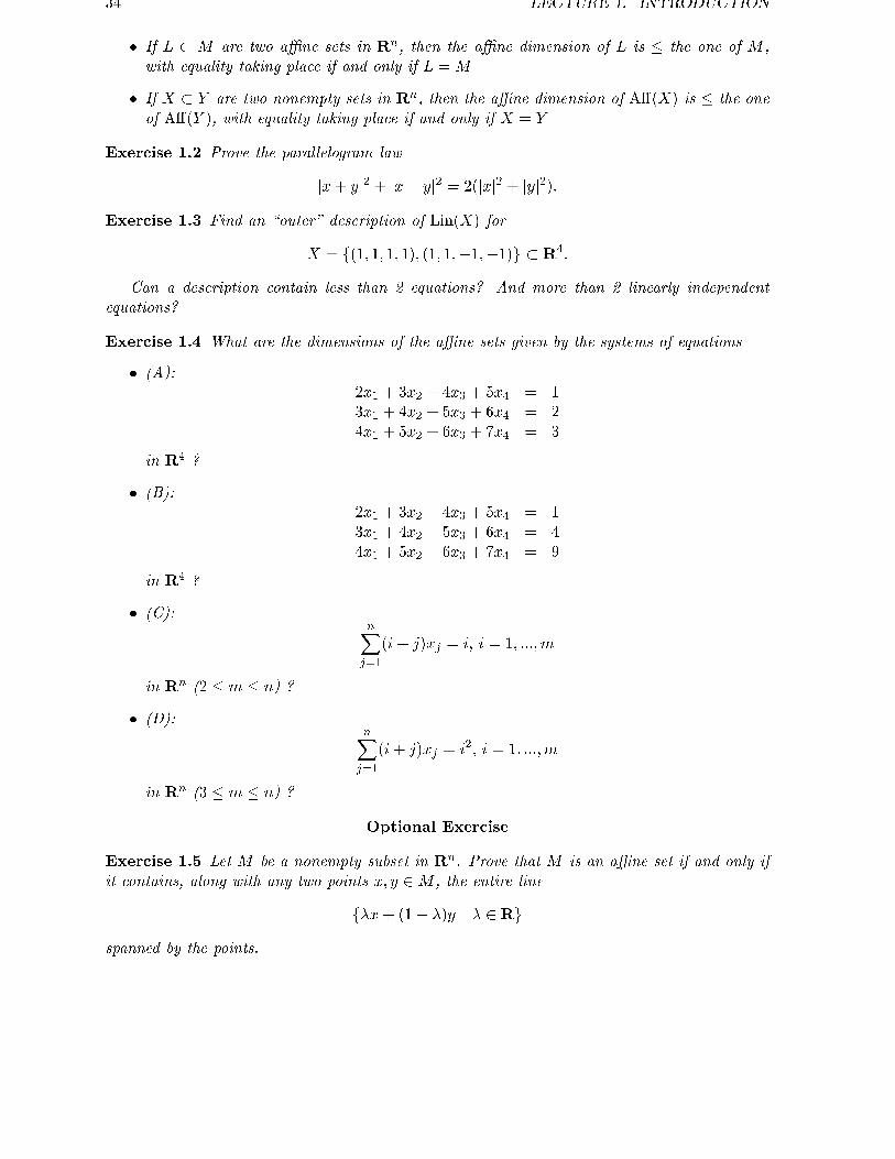
34 LECTURE 1. INTRODUCTION
� If L � M are two aÆne sets in Rn, then the aÆne dimension of L is � the one of M ,with equality taking place if and only if L =M
� If X � Y are two nonempty sets in Rn, then the aÆne dimension of A�(X) is � the oneof A�(Y ), with equality taking place if and only if X = Y
Exercise 1.2 Prove the parallelogram law
jx+ yj2 + jx� yj2 = 2(jxj2 + jyj2):Exercise 1.3 Find an \outer" description of Lin(X) for
X = f(1; 1; 1; 1); (1; 1;�1;�1)g � R4:
Can a description contain less than 2 equations? And more than 2 linearly independentequations?
Exercise 1.4 What are the dimensions of the aÆne sets given by the systems of equations
� (A):2x1 + 3x2 + 4x3 + 5x4 = 13x1 + 4x2 + 5x3 + 6x4 = 24x1 + 5x2 + 6x3 + 7x4 = 3
in R4 ?
� (B):2x1 + 3x2 + 4x3 + 5x4 = 13x1 + 4x2 + 5x3 + 6x4 = 44x1 + 5x2 + 6x3 + 7x4 = 9
in R4 ?
� (C):nXj=1
(i+ j)xj = i; i = 1; :::;m
in Rn (2 � m � n) ?
� (D):nXj=1
(i+ j)xj = i2; i = 1; :::;m
in Rn (3 � m � n) ?
Optional Exercise
Exercise 1.5 Let M be a nonempty subset in Rn. Prove that M is an aÆne set if and only ifit contains, along with any two points x; y 2M , the entire line
f�x+ (1� �)y j � 2 Rgspanned by the points.

Lecture 2
Convex sets: Introduction
Linear subspaces and aÆne sets are \too simple" to satisfy all needs of Convex Analysis. Whatwe indeed are interested in are convex sets in Rn.
2.1 De�nition, examples, inner description, algebraic properties
2.1.1 A convex set
In the school geometry a �gure is called convex if it contains, along with any pair of its pointsx; y, also the entire segment [x; y] linking the points. This is exactly the de�nition of a convexset in the multidimensional case; all we need is to say what does it mean \the segment [x; y]linking the points x; y 2 Rn". This is said by the following
De�nition 2.1.1 [Convex set]
1) Let x; y be two points in Rn. The set
[x; y] = fz = �x+ (1� �)y j 0 � � � 1g
is called a segment with the endpoints x; y.
2) A subset M of Rn is called convex, if it contains, along with any pair of its points x; y,also the entire segment [x; y]:
x; y 2M; 0 � � � 1) �x+ (1� �)y 2M:
Comment. As we know from Section 1.4.2, the set of all aÆne combinations fz = �x+(1��)y j� 2 Rg of two given vectors is their aÆne hull, which is a line, provided that x 6= y. When theparameter � of the combination is 0, we get one of the points x; y (namely, y), and when � = 1{ another of them (x). And the segment [x; y] is, in full accordance with geometric intuition, iscomprised of aÆne combinations of x; y with these extreme and all intermediate values of theparameter �.
Note that by this de�nition an empty set is convex (by convention, or better to say, by theexact sense of the de�nition: for the empty set, you cannot present a counterexample to showthat it is not convex).
35

36 LECTURE 2. CONVEX SETS: INTRODUCTION
2.1.2 Examples of convex sets
The simplest examples of nonempty convex sets are singletons { points { and the entire spaceRn. A much more interesting example is as follows:
Example 2.1.1 The solution set of an arbitrary (possibly, in�nite) system
aT�x � b�; � 2 A
of linear inequalities with n unknowns x { the set
M = fx 2 Rn j aT�x � b�; � 2 Ag
is convex.In particular, the solution set of a �nite system
Ax � b
of m inequalities with n variables (A is m�n matrix) is convex; a set of this latter type is calledpolyhedral.
Indeed, let x; y be two solutions to the system; we should prove that any point z = �x+(1��y)with � 2 [0; 1] also is a solution to the system. This is evident, since for every � 2 A we have
aT�x � b�aT�y � b�;
whence, multiplying the inequalities by nonnegative reals � and 1 � � and taking sum of theresults,
�aT�x+ (1� �)aT�y � �b� + (1� �)b� = b�;
and what is in the left hand side is exactly aT�z.
Remark 2.1.1 Note that any set given by Example 2.1.1 is not only convex, but also closed(why?)
As we remember from the previous lecture, any aÆne set in Rn (in particular, any linearsubspace) is the set of all solutions to some system of linear equations. Now, a system of linearequations is equivalent to a system of linear inequalities (you can equivalently represent a linearequality by a pair of opposite linear inequalities). It follows that an aÆne set is a particularcase of a polyhedral set and is therefore convex. Of course, we could obtain this conclusiondirectly: convexity of a set means that it is closed with respect to taking certain restrictedset of aÆne combinations of its members { namely, the pair combinations with nonnegativecoeÆcients; and aÆne set is closed with respect to taking arbitrary aÆne combinations of itselements (Proposition 1.3.2).
Our next example is as follows:
Example 2.1.2 [k � k-ball] Let k � k be a norm on Rn i.e., a real-valued function on Rn
satisfying the three characteristic properties of a norm mentioned in Section 1.1.2. Then theunit ball of this norm - the set
fx 2 E j k x k� 1g;

2.1. DEFINITION, EXAMPLES, INNER DESCRIPTION, ALGEBRAIC PROPERTIES 37
same as any other k � k-ballfx j k x� a k� rg
(a 2 Rn and r � 0 are �xed) is convex.In particular, Euclidean balls (j�j-balls associated with the standard Euclidean norm k � k= j�j)
are convex.
Indeed, let V = fx j k x � a k� rg and let x; y 2 V . We should verify that if � 2 [0; 1],then z = �x + (1� �)y 2 V . This is given by the following computation:
k z � a k = k [�x+ (1� �)y]� a k= k [�(x� a)] + [(1� �)(y � a)] k� k �(x� a) k + k (1� �)(y � a) k [triangle inequality - de�nition of a norm]= � k x� a k +(1� �) k y � a k [homogeneity - de�nition of a norm]� �r + (1� �)r = r [since x; y 2 V ]
The standard examples of norms on Rn are the lp-norms
k x kp=�(Pn
i=1 jxijp)1=p ; 1 � p <1max1�i�n jxij; p =1 :
These indeed are norms (which is not clear in advance). When p = 2, we get the usualEuclidean norm; of course, you know how the Euclidean ball looks. When p = 1, we get
k x k1=nXi=1
jxij;
and the unit ball is the hyperoctahedron
V = fx 2 Rn jnXi=1
jxij � 1g
When p =1, we getk x k1= max
1�i�njxij;
and the unit ball is the hypercube
V = fx 2 Rn j �1 � xi � 1; 1 � i � ng:It makes sense to draw the unit k � k1- and k � k1-balls in R2.
Example 2.1.3 [Ellipsoid] Let Q be a n � n matrix which is symmetric (Q = QT ) andpositive de�nite (xTQx � 0, with � being = if and only if x = 0). Then, for any nonnegativer, the Q-ellipsoid of radius r centered at a { the set
fx j (x� a)TQ(x� a) � r2gis convex.
The simplest way to prove that an ellipsoid is convex is as follows: given a positive de�nitesymmetric matrix Q, one can associate with it the Q-inner product
hx; yi = xTQy
which, as it is immediately seen, satis�es the characteristic properties { bilinearity, symmetryand positivity { of the standard inner product xT y (in fact these three properties of a Q-inner

38 LECTURE 2. CONVEX SETS: INTRODUCTION
product, taken together, are exactly equivalent to symmetry and positive de�niteness of Q).It follows that the Q-norm { the function
jxjQ =pxTQx
{ is a norm: when proving that the standard Euclidean norm is a norm (Section 1.1.2), weused bilinearity, symmetry and positivity of the standard inner product only, and no otherspeci�c properties of it). It is clearly seen that a Q-ellipsoid is nothing but a ball in the normj � jQ, so that its convexity is given by Example 2.1.2.
Example 2.1.4+[�-neighbourhood of a convex set]
Let M be a convex set in Rn, and let � > 0. Then, for any norm k � k on Rn, the �-neighbourhood of M , i.e., the set
M� = fy 2 Rn j distk�k(y;M) � infx2M
k y � x k� �g
is convex.
2.1.3 Inner description of convex sets: Convex combinations and convex hull
Convex combinations
To the moment we have de�ned the notion of linear combination y of a given set of vectorsy1; :::; ym - this is a vector represented as
y =mXi=1
�iyi;
where �i are certain real coeÆcients. Specifying this de�nition, we have come to the notion ofan aÆne combination - this is a linear combination with the sum of coeÆcients equal to one.Now we introduce the next notion in this genre: the one of convex combination.
De�nition 2.1.2 A convex combination of vectors y1; :::; ym is their aÆne combination withnonnegative coeÆcients, or, which is the same, a linear combination
y =mXi=1
�iyi
with nonnegative coeÆcients with unit sum:
�i � 0;mXi=1
�i = 1:
The following statement resembles those for linear subspaces and aÆne sets:
Proposition 2.1.1 A set M in Rn is convex if and only if it is closed with respect to taking allconvex combinations of its elements, i.e., if and only if any convex combination of vectors fromM again is a vector from M .
Proof."if" part: assume that M contains all convex combinations of the elements of M . Then,
with any two points x; y 2M and any � 2 [0; 1], M contains also the vector �x+(1��)y, sinceit is a convex combination of x and y; thus, M is convex.

2.1. DEFINITION, EXAMPLES, INNER DESCRIPTION, ALGEBRAIC PROPERTIES 39
"only if" part: assume that M is convex; we should prove that then M contains any convexcombination
(�) y =mXi=1
�iyi
of vectors yi 2M . The proof is given by induction in m. The case of m = 1 is evident (since theonly 1-term convex combinations are of the form is 1 � y1 = y1 2 M). Assume that we alreadyknow that any convex combination of m� 1 vectors, m � 2, from M is again a vector from M ,and let us prove that this statement remains valid also for all convex combinations of m vectorsfrom M . Let (*) be such a combination. We can assume that 1 > �m, since otherwise there isnothing to prove (indeed, if �m = 1, then the remaining �i's should be zero, since all �'s arenonnegative with the unit sum, and we have y = ym 2M). Assuming �m < 1, we can write
y = (1� �m)[m�1Xi=1
�i1� �m
yi] + �mym:
What is in the brackets, clearly is a convex combination of m� 1 points from M and therefore,by the inductive hypothesis, this is a point, let it be called z, from M ; we have
y = (1� �m)z + �mym
with z and ym 2M , and y 2M by de�nition of a convex set M .
Convex hull
Same as for linear subspaces and aÆne sets, we have the following fundamental, although evident,fact (completely similar to those for linear subspaces and aÆne sets):
Proposition 2.1.2 [Convexity of intersections] Let fM�g� be an arbitrary family of convexsubsets of Rn. Then the intersection
M = \�M�
is convex.
Indeed, if the endpoints of a segment [x; y] belong to M , then they belong also to every M�;due to the convexity of M�, the segment [x; y] itself belongs to every M�, and, consequently, totheir intersection, i.e., to M .
An immediate consequence of this Proposition (cf. similar statements for subspaces andaÆne sets, Lecture 1) is as follows:
Corollary 2.1.1 [Convex hull]Let M be a nonempty subset in Rn. Then among all convex sets containing M (these setsexist, e.g., Rn itself) there exists the smallest one, namely, the intersection of all convex setscontaining M .
This set is called the convex hull of M [ notation: Conv(M)].
The linear span of M is the set of all linear combinations of vectors from M , the aÆne hullis the set of all aÆne combinations of vectors from M . As you guess,
Proposition 2.1.3 [Convex hull via convex combinations] For a nonempty M � Rn:
Conv(M) = fthe set of all convex combinations of vectors from Mg:

40 LECTURE 2. CONVEX SETS: INTRODUCTION
Proof. According to Proposition 2.1.1, any convex set containing M (in particular, Conv(M))contains all convex combinations of vectors from M . What remains to prove is that Conv(M)does not contain anything else. To this end it suÆces to prove that the set of all convexcombinations of vectors from M , let this set be called M�, itself is convex (given this fact andtaking into account that Conv(M) is the smallest convex set containing M , we achieve our goal{ the inclusion Conv(M) �M�). To prove that M� is convex is the same as to prove that anyconvex combination �x + (1 � �)y of any two points x =
Pi �ixi, y =
Pi �ixi of M
� { twoconvex combinations of vectors xi 2 M { is again a convex combination of vectors from M .This is evident:
�x+ (1� �)y = �Xi
�ixi + (1� �)Xi
�ixi =Xi
�ixi; �i = ��i + (1� �)�i;
and the coeÆcients �i clearly are nonnegative with unit sum.Proposition 2.1.3 provides us with an inner (\worker's") description of a convex set. In the
mean time we shall obtain also an extremely useful outer (\artist's") description of closed convexsets: we shall prove that all these sets are given by Example 2.1.1 { they are exactly the sets ofall solutions to systems (possibly, in�nite) of nonstrict linear inequalities1).
2.1.4 More examples of convex sets: polytope and cone
\Worker's" approach to generating convex sets provides us with two seemingly new examples ofthem: { a polytope and a cone.
A polytope is, by de�nition, the convex hull of a �nite nonempty set in Rn, i.e., the set ofthe form
Conv(fu1; :::; uNg) = fNXi=1
�iui j �i � 0;Xi
�i = 1g:
An important case of a polytope is a simplex - the convex hull of n + 1 aÆnely independentpoints v1; :::; vn+1 from Rn:
M = Conv(fv1; :::; vn+1g) = fn+1Xi=1
�ivi j �i � 0;n+1Xi=1
�i = 1g;
the points v1; :::; vn+1 are called vertices of the simplex.In the mean time we shall discover that a polytope (which is de�ned via the \worker's"
approach) is nothing but a bounded polyhedral set, i.e., is a bounded set given by �nitely manylinear inequalities (this is \artists's" description of a polytope). The equivalence of these twoinner and outer de�nitions of a polytope is one of the deepest facts of Convex Analysis.
A cone. A nonempty subset M of Rn is called conic, if it contains, along with every pointx 2M , the entire ray Rx = ftx j t � 0g spanned by the point:
x 2M ) tx 2M 8t � 0:
A convex conic set is called a cone2).1)that a set of solutions to any system of nonstrict linear inequalities is closed and convex { this we already
know from Example 2.1.1 and Remark 2.1.1. The point is, of course, to prove that any closed convex set is asolution to a system of nonstrict linear inequalities
2)sometimes people call cones what we call conic sets and call convex cones what we call cones

2.1. DEFINITION, EXAMPLES, INNER DESCRIPTION, ALGEBRAIC PROPERTIES 41
Proposition 2.1.4+A nonempty subset M of Rn is a cone if and only if it possesses the
following pair of properties:
� is conic: x 2M; t � 0 ) tx 2M ;
� contains sums of its elements: x; y 2M ) x+ y 2M .
As an immediate consequence, we get that a cone is closed with respect to taking linear com-binations with nonnegative coeÆcients of the elements, and vice versa { a nonempty set closedwith respect to taking these combinations is a cone.
Example 2.1.5+The solution set of an arbitrary (possibly, in�nite) system
aT�x � 0; � 2 A
of homogeneous linear inequalities with n unknowns x { the set
K = fx j aT�x � 0 8� 2 Ag
{ is a cone.In particular, the solution set to a homogeneous �nite system of m homogeneous linear
inequalities
Ax � 0
(A is m� n matrix) is a cone; a cone of this latter type is called polyhedral.
Note that the cones given by systems of linear homogeneous nonstrict inequalities necessarily areclosed. We shall see in the mean time that, vice versa, every closed convex cone is the solutionset to such a system, so that Example 2.1.5 is the generic example of a closed convex cone.
Cones form a very important family of convex sets, and one can develop theory of conesabsolutely similar (and in a sense, equivalent) to that one of all convex sets. E.g., introducingthe notion of conic combination of vectors x1; :::; xk as a linear combination of the vectors withnonnegative coeÆcients, you can easily prove the following statements completely similar tothose for general convex sets, with conic combination playing the role of convex one:
� A set is a cone if and only if it is nonempty and is closed with respect to taking allconic combinations of its elements;
� Intersection of any family of cones is again a cone; in particular, for any nonempty setM � Rn there exists the smallest cone containing M { its conic hull Cone (M), andthis conic hull is comprised of all conic combinations of vectors from M .
In particular, the conic hull of a nonempty �nite set M = fu1; :::; uNg of vectors in Rn isthe cone
Cone (M) = fNXi=1
�iui j �i � 0; i = 1; :::; Ng:
A fundamental fact (cf. the above story about polytopes) is that this is the generic (in-
ner) description of a polyhedral cone { of a set given by (outer description) �nitely many
homogeneous linear inequalities.

42 LECTURE 2. CONVEX SETS: INTRODUCTION
2.1.5 Algebraic properties of convex sets
The following statement is an immediate consequence of the de�nition of a convex set.
Proposition 2.1.5+The following operations preserve convexity of sets:
� Arithmetic summation and multiplication by reals: if M1; :::;Mk are convex sets in Rn and�1; :::; �k are arbitrary reals, then the set
�1M1 + :::+ �kMk = fkXi=1
�ixi j xi 2Mi; i = 1; :::; kg
is convex.
� Taking the image under aÆne mapping: if M � Rn is convex and x 7! A(x) � Ax + bis an aÆne mapping from Rn into Rm (A is m � n matrix, b is m-dimensional vector),then the set
A(M) = fy = A(x) � Ax+ a j x 2Mgis a convex set in Rm;
� Taking the inverse image under aÆne mapping: if M � Rn is convex and y 7! Ay + b isan aÆne mapping from Rm to Rn (A is n �m matrix, b is n-dimensional vector), thenthe set
A�1(M) = fy 2 Rm j A(y) 2Mgis a convex set in Rm.
2.1.6 Topological properties of convex sets
Convex sets and closely related objects - convex functions - play the central role in Optimization.To play this role properly, the convexity alone is insuÆcient; we need convexity plus closedness.In Lecture 1 we have already spoken about the most basic topology-related notions { convergenceof sequences of vectors, closed and open sets in Rn. Here are three more notions we need:
The closure. It is clear from de�nition of a closed set that the intersection of any family ofclosed sets in Rn is also closed. From this fact it, as always, follows that for any subset M ofRn there exists the smallest closed set containing M ; this set is called the closure of M and isdenoted clM . In Analysis they prove the following inner description of the closure of a set in ametric space (and, in particular, in Rn):
The closure of a set M � Rn is exactly the set comprised of the limits of all convergingsequences of elements of M .
With this fact in mind, it is easy to prove that, e.g., the closure of the open Euclidean ball
fx j jx� aj < rg [r > 0]
is the closed ball fx j jx� aj � rg. Another useful application example is the closure of a set
M = fx j aT�x < b�; � 2 Aggiven by strict linear inequalities: if such a set is nonempty, then its closure is given by thenonstrict versions of the same inequalities:
clM = fx j aT�x � b�; � 2 Ag:

2.1. DEFINITION, EXAMPLES, INNER DESCRIPTION, ALGEBRAIC PROPERTIES 43
Nonemptiness of M in the latter example is essential: the set M given by two strictinequalities
x < 0; �x < 0
in R clearly is empty, so that its closure also is empty; in contrast to this, applying formallythe above rule, we would get wrong answer
clM = fx j x � 0; x � 0g = f0g:
The interior. Let M � Rn. We say that a point x 2 M is an interior point of M , if someneighbourhood of the point is contained in M , i.e., there exists centered at x ball of positiveradius which belongs to M :
9r > 0 Br(x) � fy j jy � xj � rg �M:
The set of all interior points of M is called the interior of M [notation: int M ].E.g.,
� The interior of an open set is the set itself;
� The interior of the closed ball fx j jx� aj � rg is the open ball fx j jx� aj < rg (why?)� The interior of a polyhedral set fx j Ax � bg with matrix A not containing zero rows isthe set fx j Ax < bg (why?)
The latter statement is not, generally speaking, valid for sets of solutions of in�nitesystems of linear inequalities. E.g., the system of inequalities
x � 1
n; n = 1; 2; :::
in R has, as a solution set, the nonpositive ray R� = fx � 0g; the interior of this rayis the negative ray fx < 0g. At the same time, strict versions of our inequalities
x <1
n; n = 1; 2; :::
de�ne the same nonpositive ray, not the negative one.
It is also easily seen (this fact is valid for arbitrary metric spaces, not for Rn only), that
� the interior of an arbitrary set is open
The interior of a set is, of course, contained in the set, which, in turn, is contained in its closure:
int M �M � clM: (2.1.1)
The complement of the interior in the closure { the set
@M = clMn int M{ is called the boundary of M , and the points of the boundary are called boundary points of M(Warning: these points not necessarily belong to M , since M can be less than clM ; in fact, allboundary points belong to M if and only if M = clM , i.e., if and only if M is closed).
The boundary of a set clearly is closed (as the intersection of two closed sets clM andRnn int M ; the latter set is closed as a complement to an open set, see Lecture 1). From thede�nition of the boundary,
M � int M [ @M [= clM ];
so that a point from M is either an interior, or a boundary point of M .

44 LECTURE 2. CONVEX SETS: INTRODUCTION
The relative interior. Many of the constructions to be considered possess nice properties inthe interior of the set the construction is related to and may loose these nice properties at theboundary points of the set; this is why in many cases we are especially interested in interiorpoints of sets and want the set of these points to be \enough massive". What to do if it is notthe case { e.g., there are no interior points at all (look at a segment in the plane)? It turnsout that in these cases we can use a good surrogate of the normal interior { the relative interiorde�ned as follows.
De�nition 2.1.3 [Relative interior] Let M � Rn. We say that a point x 2 M isrelative interior for M , if M contains the intersection of a small enough ball centered at xwith A�(M):
9r > 0 Br(x) \A�(M) � fy j y 2 A�(M); jy � xj � rg �M:
The set of all relative interior points of M is called its relative interior [notation: riM ].
E.g. the relative interior of a singleton is the singleton itself (since a point in the 0-dimensionalspace is the same as a ball of any positive radius); similarly, the relative interior of an aÆne setis the set itself. The interior of a segment [x; y] (x 6= y) in Rn is empty whenever n > 1; incontrast to this, the relative interior is nonempty independently of n and is the interval (x; y) {the segment with deleted endpoints. Geometrically speaking, the relative interior is the interiorwe get when regard M as a subset of its aÆne hull (the latter, geometrically, is nothing but Rk,k being the aÆne dimension of A�(M)).
We can play with the notion of the relative interior in basically the same way as with theone of interior, namely:
� since A�(M), as any aÆne set, is closed (Lecture 1, Section1.4.1) and contains M , itcontains also the smallest of closed sets containing M , i.e., clM . Therefore we have thefollowing analogies of inclusions (2.1.1):
riM �M � clM [� A�(M)]; (2.1.2)
� we can de�ne the relative boundary @riM = clMnriM which is a closed set contained inA�(M), and, as for the \actual" interior and boundary, we have
riM �M � clM = riM + @riM:
Of course, if A�(M) = Rn, then the relative interior becomes the usual interior, and similarlyfor boundary; this for sure is the case when int M 6= ; (since then M contains a ball B, andtherefore the aÆne hull of M is the entire Rn, which is the aÆne hull of B).
Nice topological properties of a convex set
An arbitrary set M in Rn may possess very pathological topology: both inclusions in the chain
riM �M � clM
can be very \non-tight". E.g., let M be the set of rational numbers in the segment [0; 1] � R.Then riM = int M = ; { since any neighbourhood of every rational real contains irrationalreals { while clM = [0; 1]. Thus, riM is \incomparably smaller" thanM , clM is \incomparablelarger", andM is contained in its relative boundary (by the way, what is this relative boundary?).
The following proposition demonstrates that the topology of a convex set M is much betterthan it might be for an arbitrary set.

2.1. DEFINITION, EXAMPLES, INNER DESCRIPTION, ALGEBRAIC PROPERTIES 45
Theorem 2.1.1 Let M be a convex set in Rn. Then(i)+The interior int M , the closure clM and the relative interior riM are convex;
(ii) If M is nonempty, then the relative interior riM of M is nonempty(iii) The closure of M is the same as the closure of its relative interior:
clM = cl riM
(in particular, every point of clM is the limit of a sequence of points from riM)(iv) The relative interior remains unchanged when we replace M with its closure:
riM = ri clM:
Proof.(ii): Let M be a nonempty convex set, and let us prove that riM 6= ;. It suÆces to consider
the case when A�(M) is the entire spaceRn. Indeed, by translation ofM we always may assumethat A�(M) contains 0, i.e., is a linear subspace. As we know from Lecture 1, a linear subspacein Rn, as far as the linear operations and the Euclidean structure are concerned, is equivalent tocertain Rk; since the notion of relative interior deals only with linear and Euclidean structures,we loose nothing thinking of A�(M) as of Rk and taking it as our universe instead of the originaluniverse Rn. Thus, in the rest of the proof of (ii) we assume that A�(M) = Rn, and what weshould prove is that the interior of M (which in the case in question is the same as relativeinterior) is nonempty.
According to Theorem 1.3.1, A�(M) = Rn possesses an aÆne basis a0; :::; an comprised ofvectors from M . Since a0; :::; an belong to M and M is convex, the entire convex hull of thevectors { the simplex � with the vertices a0; :::; an { is contained inM . Consequently, an interiorpoint of the simplex for sure is an interior point of M ; thus, in order to prove that int M 6= ;,it suÆces to prove that the interior of � is nonempty, as it should be according to geometricintuition.
The proof of the latter fact is as follows: since a0; :::; an is, by construction, an aÆne basisof Rn, every point x 2 Rn is aÆne combination of the points of the basis. The coeÆcients�i = �i(x) of the combination { the barycentric coordinates of x with respect to the basis { aresolutions to the following system of equations:
nXi=0
�iai = x;nXi=0
�i = 1;
or, in the entrywise form,
a01�0 + a11�1 + ::: + an1�n = x1a02�0 + a12�1 + ::: + an2�n = x2::::: ::::: ::::: ::::: = :::
a0n�0 + a1n�1 + ::: + ann�n = xn�0 + �2 + ::: + �n = 1
; (2.1.3)
(apq is q-th entry of vector ap). This is a linear system of equations with n + 1 equation andn + 1 unknown. The corresponding homogeneous system has only trivial solution { indeed, anontrivial solution to the homogeneous system would give us an equal to zero nontrivial linearcombination of ai with zero sum of coeÆcients, while from aÆne independence of a0; :::; an (theyare aÆne independent since they form an aÆne basis) we know that no such a combination

46 LECTURE 2. CONVEX SETS: INTRODUCTION
exists. It follows that the matrix of the system, let it be called A, is nonsingular, so that thesolution �(x) linearly (consequently, continuously) depends on the right hand side data, i.e., onx.
Now we are done: let us take any x = x0 with �i(x0) > 0, e.g., x0 = (n + 1)�1Pn
i=0 ai.Due to the continuity of �i(�)'s, there is a neighbourhood of x0 { a centered at x0 ball Br(x0) ofpositive radius r - where the functions �i still are positive:
x 2 Br(x0)) �i(x) � 0; i = 0; :::; n:
The latter relation means that every x 2 Br(x0) is an aÆne combination of ai with positivecoeÆcients, i.e., is a convex combination of the vectors, and therefore x belongs to �. Thus, �contains a neighbourhood of x0, so that x0 is an interior point of �.
(iii): We should prove that the closure of riM is exactly the same that the closure of M . Infact we shall prove even more:
Lemma 2.1.1 Let x 2 riM and y 2 clM . Then all points from the half-segment [x; y),
[x; y) = fz = (1� �)x+ �y j 0 � � < 1g
belong to the relative interior of M .
Proof of the Lemma. Let A�(M) = a+ L, L being linear subspace; then
M � A�(M) = x+ L:
Let B be the unit ball in L:B = fh 2 L j k h k� 1g:
Since x 2 riM , there exists positive radius r such that
x+ rB �M: (2.1.4)
Since y 2 clM , we have y 2 A�(M) (see (2.1.2)). Besides this, for any � > 0 there exists y0 2Msuch that jy0 � yj � �; since both y0 and y belong to A�(M), the vector y� y0 belongs to L andconsequently to �B. Thus,
(8� > 0) : y 2M + �B: (2.1.5)
Now let z 2 [x; y), so thatz = (1� �)x+ �y
with some � 2 (0; 1); we should prove that z is relative interior for M , i.e., that there existsr0 > 0 such that
z + r0B �M: (2.1.6)
For any � > 0 we have, in view of (2.1.5),
z+ �B � (1��)x+�y+ �B � (1��)x+�[M + �B]+ �B = (1��)[x+ ��
1� �B+
�
1� �B]+�M
(2.1.7)for all � > 0. Now, for the centered at zero Euclidean ball B and nonnegative t0; t00 one has
t0B + t00B � (t0 + t00)B
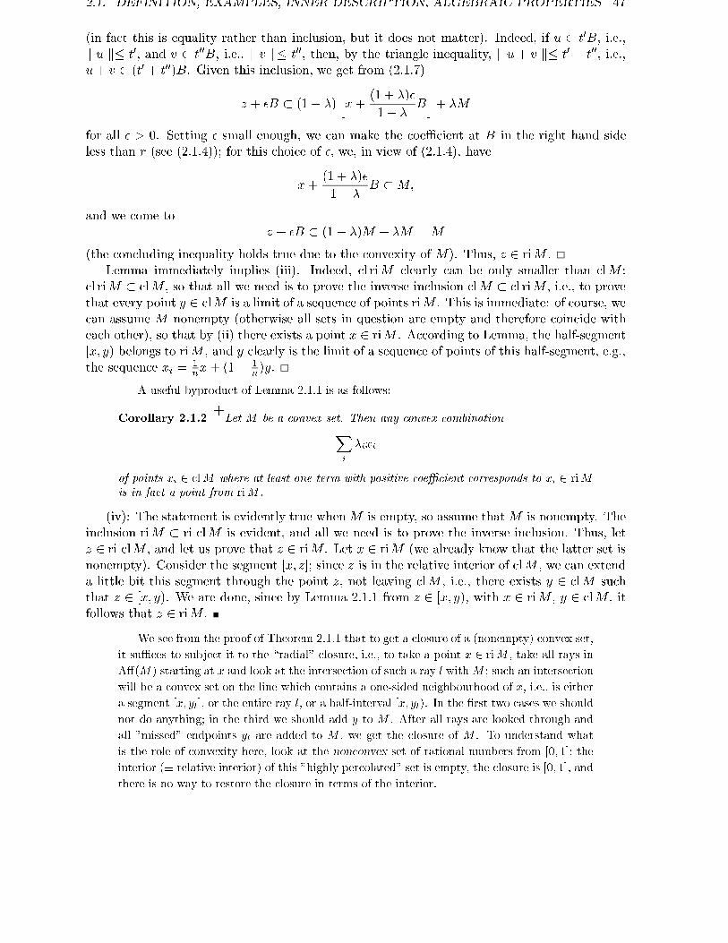
2.1. DEFINITION, EXAMPLES, INNER DESCRIPTION, ALGEBRAIC PROPERTIES 47
(in fact this is equality rather than inclusion, but it does not matter). Indeed, if u 2 t0B, i.e.,k u k� t0, and v 2 t00B, i.e., k v k� t00, then, by the triangle inequality, k u+ v k� t0 + t00, i.e.,u+ v 2 (t0 + t00)B. Given this inclusion, we get from (2.1.7)
z + �B � (1� �)�x+
(1 + �)�
1� �B�+ �M
for all � > 0. Setting � small enough, we can make the coeÆcient at B in the right hand sideless than r (see (2.1.4)); for this choice of �, we, in view of (2.1.4), have
x+(1 + �)�
1� �B �M;
and we come toz + �B � (1� �)M + �M =M
(the concluding inequality holds true due to the convexity of M). Thus, z 2 riM .Lemma immediately implies (iii). Indeed, cl riM clearly can be only smaller than clM :
cl riM � clM , so that all we need is to prove the inverse inclusion clM � cl riM , i.e., to provethat every point y 2 clM is a limit of a sequence of points riM . This is immediate: of course, wecan assume M nonempty (otherwise all sets in question are empty and therefore coincide witheach other), so that by (ii) there exists a point x 2 riM . According to Lemma, the half-segment[x; y) belongs to riM , and y clearly is the limit of a sequence of points of this half-segment, e.g.,the sequence xi =
1nx+ (1 � 1
n)y.
A useful byproduct of Lemma 2.1.1 is as follows:
Corollary 2.1.2+Let M be a convex set. Then any convex combinationX
i
�ixi
of points xi 2 clM where at least one term with positive coeÆcient corresponds to xi 2 riMis in fact a point from riM .
(iv): The statement is evidently true whenM is empty, so assume that M is nonempty. Theinclusion riM � ri clM is evident, and all we need is to prove the inverse inclusion. Thus, letz 2 ri clM , and let us prove that z 2 riM . Let x 2 riM (we already know that the latter set isnonempty). Consider the segment [x; z]; since z is in the relative interior of clM , we can extenda little bit this segment through the point z, not leaving clM , i.e., there exists y 2 clM suchthat z 2 [x; y). We are done, since by Lemma 2.1.1 from z 2 [x; y), with x 2 riM , y 2 clM , itfollows that z 2 riM .
We see from the proof of Theorem 2.1.1 that to get a closure of a (nonempty) convex set,
it suÆces to subject it to the \radial" closure, i.e., to take a point x 2 riM , take all rays in
A�(M) starting at x and look at the intersection of such a ray l withM ; such an intersection
will be a convex set on the line which contains a one-sided neighbourhood of x, i.e., is either
a segment [x; yl], or the entire ray l, or a half-interval [x; yl). In the �rst two cases we should
not do anything; in the third we should add y to M . After all rays are looked through and
all "missed" endpoints yl are added to M , we get the closure of M . To understand what
is the role of convexity here, look at the nonconvex set of rational numbers from [0; 1]; the
interior (� relative interior) of this "highly percolated" set is empty, the closure is [0; 1], and
there is no way to restore the closure in terms of the interior.
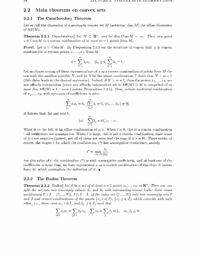
48 LECTURE 2. CONVEX SETS: INTRODUCTION
2.2 Main theorems on convex sets
2.2.1 The Caratheodory Theorem
Let us call the dimension of a nonempty convex set M (notation: dim M) the aÆne dimensionof A�(M).
Theorem 2.2.1 [Caratheodory] Let M � Rn, and let dim ConvM = m. Then any pointx 2 ConvM is a convex combination of at most m+ 1 points from M .
Proof. Let x 2 ConvM . By Proposition 2.1.3 on the structure of convex hull, x is convexcombination of certain points x1; :::; xN from M :
x =NXi=1
�ixi; [�i � 0;NXi=1
�i = 1]:
Let us choose among all these representations of x as a convex combination of points fromM theone with the smallest possible N , and let it be the above combination. I claim that N � m+ 1(this claim leads to the desired statement). Indeed, if N > m+1, then the points x1; :::; xN arenot aÆnely independent (since any aÆnely independent set in A�(M) � M is comprised of atmost dim A�(M) + 1 = m+ 1 points, Proposition 1.3.5). Thus, certain nontrivial combinationof x1; :::; xN with zero sum of coeÆcients is zero:
NXi=1
Æixi = 0; [NXi=1
Æi = 0; (Æ1; :::; ÆN ) 6= 0]:
It follows that, for any real t,
(�)NXi=1
[�i + tÆi]xi = x:
What is to the left, is an aÆne combination of xi's. When t = 0, this is a convex combination- all coeÆcients are nonnegative. When t is large, this is not a convex combination, since someof Æi's are negative (indeed, not all of them are zero, and the sum of Æi's is 0). There exists, ofcourse, the largest t for which the combination (*) has nonnegative coeÆcients, namely
t� = mini:Æi<0
�ijÆij :
For this value of t, the combination (*) is with nonnegative coeÆcients, and at least one of thecoeÆcients is zero; thus, we have represented x as a convex combination of less than N pointsfrom M , which contradicts the de�nition of N .
2.2.2 The Radon Theorem
Theorem 2.2.2 [Radon] Let S be a set of at least n+2 points x1; :::; xN in Rn. Then one cansplit the set into two nonempty subsets S1 and S2 with intersecting convex hulls: there existspartitioning I [ J = f1; :::; Ng, I \ J = ;, of the index set f1; :::; Ng into two nonempty sets Iand J and convex combinations of the points fxi; i 2 Ig, fxj ; j 2 Jg which coincide with eachother, i.e., there exist �i; i 2 I, and �j ; j 2 J , such thatX
i2I
�ixi =Xj2J
�jxj;Xi
�i =Xj
�j = 1; �i; �j � 0:

2.2. MAIN THEOREMS ON CONVEX SETS 49
Proof. Since N > n + 1, the points x1; :::; xN are not aÆnely independent (since in Rn, aswe know, e.g. from Proposition 1.3.5, any aÆne independent set contains no more than n + 1point). Thus, there exists a nontrivial combination of xi's with zero sum of coeÆcients which isequal to 0:
NXi=1
�ixi = 0; [NXi=1
�i = 0; (�1; :::; �N ) 6= 0]:
Let I = fi j �i � 0g, J = fi j �i < 0g; then I and J are nonempty and form a partitioning off1; :::; Ng. We have
a �Xi2I
�i =Xj2J
(��j) > 0
(since the sum of all �'s is zero and not all �'s are zero). Setting
�i =�ia; i 2 I; �j = ��j
a; j 2 J;
we get�i � 0; �j � 0;
Xi2I
�i = 1;Xj2J
�j = 1;
and
[Xi2I
�ixi]� [Xj2J
�jxj ] = a�1
0@[Xi2I
�ixi]� [Xj2J
(��j)xj ]1A = a�1
NXi=1
�ixi = 0:
2.2.3 The Helley Theorem
Theorem 2.2.3 [Helley, I] Let F be a �nite family of convex sets in Rn. Assume that any n+1sets from the family have a point in common. The all the sets have a point in common.
Proof. Let us prove the statement by induction of the number N of sets in the family. Thecase of N � n + 1 is evident. Now assume that we have proved the statement for all familieswith certain number N � n + 1 of sets, and let S1; :::; SN ; SN+1 be a family of N + 1 convexsets which satis�es the premise of the Helley Theorem; we should prove that the intersection ofthe sets S1; :::; SN ; SN+1 is nonempty.
Deleting from our N+1-set family the set Si, we get N -set family which satis�es the premiseof the Helley theorem and thus, by the inductive hypothesis, possesses a nonempty intersectionof its members:
(8i � N + 1) : T i = S1 \ S2 \ ::: \ Si�1 \ Si+1 \ ::: \ SN+1 6= ;:Let us choose a point xi in the (nonempty) set T i. We get N +1 � n+2 points from Rn. As weknow from Radon's Theorem, we can partition the index set f1; :::; N + 1g into two nonemptysubsets I and J in such a way that certain convex combination x of the points xi, i 2 I, issimultaneously a convex combination of the points xj , j 2 J . Let us verify that x belongs to allthe sets S1; :::; SN+1, which will complete the proof. Indeed, let i� be an index from our indexset; let us prove that x 2 Si� . We have either i� 2 I, or i� 2 J . In the �rst case all the setsT j, j 2 J , are contained in Si� (since Si� participates in all intersections which give T i withi 6= i�). Consequently, all the points xj , j 2 J , belong to Si� , and therefore x, which is a convexcombination of these points, also belongs to Si� (all our sets are convex!), as required. In thesecond case similar reasoning says that all the points xi, i 2 I, belong to Si� , and therefore x,which is a convex combination of these points, belongs to Si�

50 LECTURE 2. CONVEX SETS: INTRODUCTION
In the aforementioned version of the Helley theorem we dealt with �nite families of convexsets. To extend the statement to the case of in�nite families, we need to strengthen slightlythe assumption. The resulting statement is as follows:
Theorem 2.2.4�[Helley, II] Let F be an arbitrary family of convex sets in Rn. Assume
that(a) every n+ 1 sets from the family have a point in common,
and(b) every set in the family is closed, and the intersection of the sets from certain �nite
subfamily of the family is bounded (e.g., one of the sets in the family is bounded).Then all the sets from the family have a point in common.
Proof�. By the previous theorem, all �nite subfamilies of F have nonempty intersections,
and these intersections are convex (since intersection of any family of convex sets is convex,Theorem 2.1.2); in view of (a) these intersections are also closed. Adding to F all intersectionsof �nite subfamilies of F , we get a larger family F 0 comprised of closed convex sets, and any�nite subfamily of this larger family again has a nonempty intersection. Besides this, from(b) it follows that this new family contains a bounded set Q. Since all the sets are closed,the family of sets
fQ \Q0 j Q0 2 Fgis a nested family of compact sets (i.e., a family of compact sets with nonempty intersection
of any �nite subfamily); by the well-known Analysis theorem such a family has a nonempty
intersection3).
3)here is the proof of this Analysis theorem: assume, on contrary, that the compact sets Q�, � 2 A, in questionhave empty intersection. Choose a set Q�� from the family; for every x 2 Q�� there is a set Qx in the familywhich does not contain x - otherwise x would be a common point of all our sets. Since Qx is closed, there is anopen ball Vx centered at x which does not intersect Qx. The balls Vx, x 2 Q�� , form an open covering of thecompact set Q�� , and therefore there exists a �nite subcovering Vx1 ; :::; VxN of Q�� by the balls from the covering.Since Qxi does not intersect Vxi , we conclude that the intersection of the �nite subfamily Q�� ; Q
x1 ; :::; QxN isempty, which is a contradiction

2.2. MAIN THEOREMS ON CONVEX SETS 51
Assignment # 2 (Lecture 2)
Exercise 2.1 Which of the following sets are convex:
� fx 2 Rn j Pni=1 x
2i = 1g
� fx 2 Rn j Pni=1 x
2i � 1g
� fx 2 Rn j Pni=1 x
2i � 1g
� fx 2 Rn j maxi=1;:::;n xi � 1
� fx 2 Rn j maxi=1;:::;n xi � 1
� fx 2 Rn j maxi=1;:::;n xi = 1
� fx 2 Rn j mini=1;:::;n xi � 1
� fx 2 Rn j mini=1;:::;n xi � 1
� fx 2 Rn j mini=1;:::;n xi = 1
Do at least 3, on your choice, of the following 5 exercises 2.2 - 2.6:
Exercise 2.2 Prove Proposition 2.1.4.
Exercise 2.3 Prove the statement contained in Example 2.1.5.
Exercise 2.4 Prove Proposition 2.1.5.
Exercise 2.5 Prove item (i) of Theorem 2.1.1.
Exercise 2.6 Prove Corollary 2.1.2.
Exercise 2.7 (!) Prove the following Kirchberger's Theorem:
Assume that X = fx1; :::; xkg and Y = fy1; :::; ymg are �nite sets in Rn, with k+m � n+2,and all the points x1; :::; xk; y1; :::; ym are distinct. Assume that for any subset S � X [ Ycomprised of n+ 2 points the convex hulls of the sets X \ S and Y \ S do not intersect. Thenthe convex hulls of X and Y also do not intersect.
Hint: assume, on contrary, that the convex hulls of X and Y intersect, so that
kXi=1
�ixi =mXj=1
�jyj
for certain nonnegative �i,P
i �i = 1, and certain nonnegative �j,P
j �j = 1, and look at theexpression of this type with the minimum possible total number of nonzero coeÆcients �i, �j.

52 LECTURE 2. CONVEX SETS: INTRODUCTION
Optional exercises
Exercise 2.8 Prove the following Grunbaum's theorem on mass partitioning:
Assume that x1; :::; xN are points from Rn, and every point xi is assigned a nonnegative mass�i, the sum of the masses of all points being equal to 1. Then there exists a point x� such thatany hyperplane fx j aTx = aTx�g, a 6= 0, passing through the point x� splits the space Rn intotwo closed half-spaces of the mass at least 1
n+1 each, i.e., that for any a 6= 0 one has
Xij aT xi�aT x�
�i � 1
n+ 1
and XijaT xi�aT x�
�i � 1
n+ 1:

Lecture 3
Separation Theorem. Theory oflinear inequalities
The theorems we are coming to answer the following question: assume we are given two convexsets in Rn. When can we separate them by a hyperplane, i.e., to �nd a nonzero linear formwhich at any point of one of the sets is greater than or equal to its value on any point of theother set? The theorems might look strange at the �rst glance: why should we be interested inthis question? But we shall see that these theorems form, in a sense, the heart, or, better tosay, the basis of the entire Convex Analysis; they will underlie all our further developments.
3.1 The Separation Theorem
Let us start with de�nitions. A hyperplane M in Rn (an aÆne set of dimension n� 1), as weknow from Section 1.4.2, is nothing but a level set of a nontrivial linear form:
9a 2 Rn; b 2 R; a 6= 0 : M = fx 2 Rn j aTx = bg:
We can, consequently, associate with the hyperplane (or, better to say, with the associated linearform a; this form us de�ned uniquely, up to multiplication by a nonzero real) the following sets:
� "upper" and "lower" open half-spaces M++ = fx 2 Rn j aTx > bg, M�� = fx 2 Rn jaTx < bg;these sets clearly are convex, and since a linear form is continuous, and the sets are givenby strict inequalities on the value of a continuous function, they indeed are open.
Note that since a is uniquely de�ned by M , up to multiplication by a nonzero real, theseopen half-spaces are uniquely de�ned by the hyperplane, up to swapping the "upper" andthe "lower" ones (which half-space is "upper", it depends on the particular choice of a);
� "upper" and "lower" closed half-spaces M+ = fx 2 Rn j aTx � bg, M� = fx 2 Rn jaTx � bg;these are also convex sets, now closed (since they are given by non-strict inequalities onthe value of a continuous function). It is easily seen that the closed upper/lower half-spaceis the closure of the corresponding open half-space, and M itself is the boundary (i.e., thecomplement of the interior to the closure) of all four half-spaces.
53
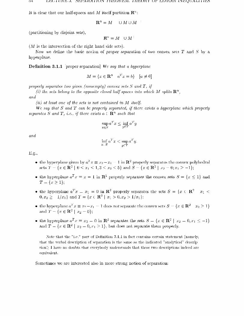
54 LECTURE 3. SEPARATION THEOREM. THEORY OF LINEAR INEQUALITIES
It is clear that our half-spaces and M itself partition Rn:
Rn =M�� [M [M++
(partitioning by disjoint sets),Rn =M� [M+
(M is the intersection of the right hand side sets).Now we de�ne the basic notion of proper separation of two convex sets T and S by a
hyperplane.
De�nition 3.1.1 [proper separation] We say that a hyperplane
M = fx 2 Rn j aTx = bg [a 6= 0]
properly separates two given (nonempty) convex sets S and T , if(i) the sets belong to the opposite closed half-spaces into which M splits Rn,
and(ii) at least one of the sets is not contained in M itself.We say that S and T can be properly separated, if there exists a hyperplane which properly
separates S and T , i.e., if there exists a 2 Rn such that
supx2S
aTx � infy2T
aT y
andinfx2S
aTx < supy2T
aT y:
E.g.,
� the hyperplane given by aTx � x2�x1 = 1 inR2 properly separates the convex polyhedralsets T = fx 2 R2 j 0 � x1 � 1; 3 � x2 � 5g and S = fx 2 R2 j x2 = 0;x1 � �1g;
� the hyperplane aTx � x = 1 in R1 properly separates the convex sets S = fx � 1g andT = fx � 1g;
� the hyperplane aTx � x1 = 0 in R2 properly separates the sets S = fx 2 R2 j x1 <0; x2 � �1=x1g and T = fx 2 R2 j x1 > 0; x2 > 1=x1g;
� the hyperplane aTx � x2�x1 = 1 does not separate the convex sets S = fx 2 R2 j x2 � 1gand T = fx 2 R2 j x2 = 0g;
� the hyperplane aTx � x2 = 0 in R2 separates the sets S = fx 2 R2 j x2 = 0; x1 � �1gand T = fx 2 R2 j x2 = 0; x1 � 1g, but does not separate them properly.
Note that the "i.e." part of De�nition 3.1.1 in fact contains certain statement (namely,
that the verbal description of separation is the same as the indicated "analytical" descrip-
tion); I have no doubts that everybody understands that these two descriptions indeed are
equivalent.
Sometimes we are interested also in more strong notion of separation:

3.1. THE SEPARATION THEOREM 55
De�nition 3.1.2 [strong separation] We say that two nonempty sets S and T in Rn can bestrongly separated, if there exist two distinct parallel hyperplanes which separate S and T , i.e.,if there exists a 2 Rn such that
supx2S
aTx < infy2T
aT y:
It is clear that
Strong separation ) Proper separation
We can immediately point out examples of the sets which can be separated properly andcannot be separated strongly, e.g., the sets fx 2 R2 j x1 > 0; x2 � 1=x1g and fx 2 R2 j x1 <0; x2 � �1=x1g.
Now we come to the most important for us question:
when a given pair of nonempty convex sets S and T in Rn can be separated [properly,strongly]?
The most important question is that one on the possibility of proper separation. The answeris as follows:
Theorem 3.1.1 [Separation Theorem] Two nonempty convex sets S, T in Rn can be properlyseparated if and only if their relative interiors are disjoint:
riS \ riT = ;:The remaining part of the Section is devoted to the proof of this fundamental theorem.
3.1.1 Necessity
The necessity of the indicated property (the "only if" part of the Separation Theorem) is moreor less evident. Indeed, assume that the sets can be properly separated, so that for certainnonzero a 2 Rn we have
supx2S
aTx � infy2T
aT y; infx2S
aTx < supy2T
aT y: (3.1.1)
We should lead to a contradiction the assumption that riS and riT have in common certainpoint �x. Assume that it is the case; then from the �rst inequality in (3.1.1) it is clear that �xmaximizes the linear function f(x) = aTx on S and simultaneously minimizes this function onT . Now, we have the following simple and important
Lemma 3.1.1 A linear function f(x) = aTx can attain its maximum/minimumover a convex set Q at a point x 2 riQ if and only if the function is constant on Q.
Proof. "if" part is evident. To prove the "only if" part, let �x 2 riQ be, say,a minimizer of f over Q and y be an arbitrary point of Q; we should prove thatf(�x) = f(y). There is nothing to prove if y = �x, so let us assume that y 6= �x. Since�x 2 riQ, the segment [y; �x], which is contained in M , can be extended a little bitthrough the point �x, not leaving M (since �x 2 riQ), so that there exists z 2 Q suchthat �x 2 [y; z), i.e., �x = (1 � �)y + �z with certain � 2 (0; 1]; since y 6= �x, we havein fact � 2 (0; 1). Since f is linear, we have
f(�x) = (1� �)f(y) + �f(z);
since f(�x) � minff(y); f(z)g and 0 < � < 1, this relation can be satis�ed only whenf(�x) = f(y) = f(z).

56 LECTURE 3. SEPARATION THEOREM. THEORY OF LINEAR INEQUALITIES
Coming back to our considerations related to (3.1.1), we conclude from Lemma that underour assumption (9�x 2 riS \ riT , i.e., when f(x) = aTx attains it maximum over S and itsminimum over T at �x) f is constant (and equal to aT �x) on both S and T ; but this contradictsthe second inequality in (3.1.1).
Thus, we have proved that the condition riS \ riT = ; is necessary for proper separation ofS and T .
3.1.2 SuÆciency
The proof of suÆciency part of the Separation Theorem is much more instructive. There areseveral ways to prove it, and I choose the one which goes via The Farkas Lemma, which isextremely important in its own right.
The Homogeneous Farkas Lemma
Let a1; :::; aN be vectors from Rn, and let a be another vector. Let us pose the question: whena belongs to the cone spanned by the vectors a1; :::; aN , i.e., can be represented as a linearcombination of ai with nonnegative coeÆcients? A necessary condition is evident: if
a =nXi=1
�iai [�i � 0; i = 1; :::; N ]
then any vector h which has nonnegative inner products with all ai should also have nonnegativeinner product with a:
a =Xi
�iai & �i � 08i & hT ai � 08i) hTa � 0:
The Homogeneous Farkas Lemma says that this evident necessary condition is also suÆcient:
Lemma 3.1.2 [Homogeneous Farkas Lemma] Let a; a1; :::; aN be vectors from Rn. The vectora is a conic combination of the vectors ai (linear combination with nonnegative coeÆcients) ifand only if every vector h satisfying hT ai � 0, i = 1; :::; N , satis�es also hT a � 0.
Proof. The necessity { the \only if" part { was already proved. Let us prove the \if" part, i.e.,assume that every vector h satisfying hTai � 0 8i satis�es also hT a � 0, and let us prove thata is a conic combination of the vectors ai.
There is nothing to prove when a = 0 { the zero vector of course is a conic combination ofthe vectors ai. Thus, from now on we assume that a 6= 0.
10. Let� = fh j aTh = �1g;
and letAi = fh 2 � j aTi h � 0g:
� is a hyperplane in Rn, and every Ai is a polyhedral set contained in this hyperplane and istherefore convex.
20. What we know is that the intersection of all the sets Ai, i = 1; :::; N , is empty (since avector h from the intersection would have nonnegative inner products with all ai and the innerproduct �1 with a, and we are given that no such h exists). Let us choose the smallest, in thenumber of elements, of those sub-families of the family of sets A1; :::; AN which still have empty

3.1. THE SEPARATION THEOREM 57
intersection of their members; without loss of generality we may assume that this is the familyA1; :::; Ak. Thus, the intersection of all k sets A1; :::; Ak is empty, but the intersection of anyk � 1 sets from the family A1; :::; Ak is nonempty.
30. I claim that
� A. a 2 Lin(fa1; :::; akg);� B. The vectors a1; :::; ak are linearly independent.
A. is easy: assuming that a 62 E = Lin(fa1; :::; akg), we conclude that the or-thogonal projection f of the vector a onto the orthogonal complement E? to E isnonzero. The inner product of f and a is the same as fTf , is.e., is positive, whilefTai = 0, i = 1; :::; k. Taking h = �(fT f)�1f , we see that hT a = �1 and hTai = 0,i = 1; :::; k. In other words, h belongs to every set Ai, i = 1; :::; k, by de�nition ofthese sets, and therefore the intersection of the sets A1; :::; Ak is nonempty, which isa contradiction.
B. is given by the Helley Theorem I. Indeed, assume that a1; :::; ak are linearlydependent, and let us lead this assumption to a contradiction. Since a1; :::; ak arelinearly dependent, the dimension of E = Lin(fa1; :::; akg) is certain m < k. Wealready know from A. that a 2 E. Now let A0i = Ai \ E. I claim that everyk � 1 of the sets A0i have a nonempty intersection, while all k these sets have emptyintersection. The second claim is evident { since A1; :::; Ak have empty intersection,the same is the case with their parts A0i. The �rst claim also is easily supported: letus take k � 1 of the dashed sets, say, A01; :::; A
0k�1. By construction, the intersection
of A1; :::; Ak�1 is nonempty; let h be a vector from this intersection, i.e., a vectorwith nonnegative inner products with a1; :::; ak�1 and the product �1 with a. Whenreplacing h with its orthogonal projection h0 on E, we do not vary all these innerproducts, since these are products with vectors from E; thus, h0 also is a commonpoint of A1; :::; Ak�1, and since this is a point from E, it is a common point of thedashed sets A01; :::; A
0k�1 as well.
Now we can complete the proof of B.: the sets A01; :::; A0k are convex sets belonging
to the hyperplane �0 = � \ E = fh 2 E j aTh = �1g (E indeed is a hyperplane inE, since 0 6= a 2 E) in the m-dimensional linear subspace E. �0 is an aÆne set ofthe dimension l = dim E � 1 = m � 1 < k � 1 (recall that we are in the situationwhen m = dim E < k), and every l + 1 � k � 1 of convex subsets A01,...,A
0k of �0
have a nonempty intersection. From the Helley Theorem I (which of course is validfor convex subsets of an aÆne set, the aÆne dimension of the set playing the role ofn in the original formulation) it follows that all the sets A01; :::; A
0k have a point in
common, which, as we know, is not the case. The contradiction we have got provesthat a1; :::; ak are linearly independent.
40. With A. and B. in our disposal, we can easily complete the proof of the \if" part of theFarkas Lemma as follows: by A., we have
a =kXi=1
�iai
with some real coeÆcients �i, and all we need is to prove that these coeÆcients are nonnegative.Assume, on contrary, that, say, �1 < 0. Let us extend the (linearly independent by B.) system

58 LECTURE 3. SEPARATION THEOREM. THEORY OF LINEAR INEQUALITIES
of vectors a1; :::; ak by vectors f1; :::; fn�k to a basis in Rn (which is possible by Theorem 1.2.1)
and let �i(x) be the coordinates of a vector x in this basis (�1 corresponds to a1). The function�1(x) is a linear form of x and therefore, according to Section 1.1.2, is the inner product withcertain vector:
�1(x) = fTx 8x:Now we have
fTa = �1(a) = �1 < 0
and
fTai =�1; i = 10; i = 2; :::; k
so that fTai � 0, i = 1; :::; k. We conclude that a proper normalization of f { namely, thevector j�1j�1f { belongs to A1; :::; Ak, which is the desired contradiction { by construction, thisintersection is empty.
Remark 3.1.1 An immediate corollary of the Homogeneous Farkas Lemma is that the conichull
Cone (fa1; :::; aNg) = fa =NXi=1
�iai j �i � 0; i = 1; :::; Ng
of a �nite nonempty set is the set of all solutions to certain system of homogeneous nonstrictlinear inequalities, namely, the system
fhT a � 0 8(h : hT ai � 0; i = 1; :::; N)g:It follows that the conic hull of a �nite set of vectors is not only convex, but also closed.
In the next Lecture we shall establish much stronger result: the conic hull of a �nite nonemptyset is a polyhedral cone, i.e., is given by �nite system of homogeneous nonstrict linear inequalities.
From Farkas' Lemma to Separation Theorem
Now we are enough equipped to prove the suÆciency part of the Separation Theorem.
Step 1. Separation of a convex polytope and a point outside the polytope. Let usstart with seemingly very particular case of the Separation Theorem { that where one of thesets is a polytope { the convex full of �nite set of points x1; :::; xN { and the other one is asingleton T = fxg. What we should prove is that if x 62 S = Conv(fx1; :::; xNg), then thereexists a linear form which properly separates x and S; in fact we shall prove even the existenceof strong separation.
Let us associate with n-dimensional vectors x1; :::; xN ; x the (n + 1)-dimensional vectors
a =�x1
�and ai =
�xi1
�, i = 1; :::; N . I claim that a does not belong to the conic hull
of a1; :::; aN . Indeed, if a would be representable as a linear combination of a1; :::; aN withnonnegative coeÆcients, then, looking at the last, (n+1)-st, coordinates in such a representation,we would conclude that the sum of coeÆcients should be 1, so that the representation, actually,represents x as a convex combination of x1; :::; xN , which was assumed to be impossible.
Since a does not belong to the conic hull of a1; :::; aN , then by the Homogeneous Farkas
Lemma, there exists a vector h =�f�
�2 Rn+1 which \separates" a and a1; :::; aN in the sense
thathTa > 0; hT ai � 0; i = 1; :::; N;

3.1. THE SEPARATION THEOREM 59
whence, of course,hTa > max
ihTai:
Since the components in all the inner products hTa; hT ai coming from the (n+1)-st coordinatesare equal to each other , we conclude that the n-dimensional component f of h separates x andx1; :::; xN :
[hT a� � =] fTx > maxifTxi [= max
ihT ai � �]:
Since for any convex combination y =P
i �ixi of the points xi one clearly has fTy � maxi fTxi,
we conclude, �nally, thatfTx > max
y2Conv(fx1;:::;xNg)fTy;
so that f strongly separates T = fxg and S = Conv(fx1; :::; xNg).Remark 3.1.2 A byproduct of our reasoning is that a polytope { the convex hull
Conv(fv1; :::; vNg)of a �nite nonempty set of vectors { is the set of solutions to a system of nonstrict linearinequalities { namely, the system
ffTx � maxi=1;:::;N
fTvi 8fg:
It follows that a polytope is not only convex, but also a closed set. In the next Lecture we shallobtain a much stronger result: a polytope is a polyhedral set { the one given by �nitely manynonstrict linear inequalities. In fact, polytopes are exactly the same as bounded and nonemptypolyhedral set.
Step 2. Separation of a convex set and a point outside of the set. Now consider thecase when S is an arbitrary nonempty convex set and T = fxg is a singleton outside S (thedi�erence with Step 1 is that now S is not assumed to be a polytope).
First of all, without loss of generality we may assume that S contains 0 (if it is not the case,we may subject S and T to translation S 7! a + S, T 7! a + T with a 2 �S). Let L be thelinear span of S. If x 62 L, the separation is easy: taking as f the orthogonal to L component ofx, we shall get
fTx = fTf > 0 = maxy2S
fTy;
so that f strongly separates S and T = fxg.It remains to consider the case when x 2 L. Since S � L, x 2 L and x 62 S, L is a nonzero
linear subspace. Let � = fh 2 L j jhj = 1g be the unit sphere in L. This is a closed andbounded set in Rn (boundedness is evident, and closedness follows from the fact that j � j iscontinuous and L is closed, see Section 1.4.1). Consequently, � is a compact set (Proposition1.1.1). Let us prove that there exists f 2 � which separates x and S in the sense that
fTx � supy2S
fTy: (3.1.2)
Assume, on contrary, that no such f exists, and let us lead this assumption to a contradiction.Under our assumption for every h 2 � there exists yh 2 S such that
hT yh > hTx:
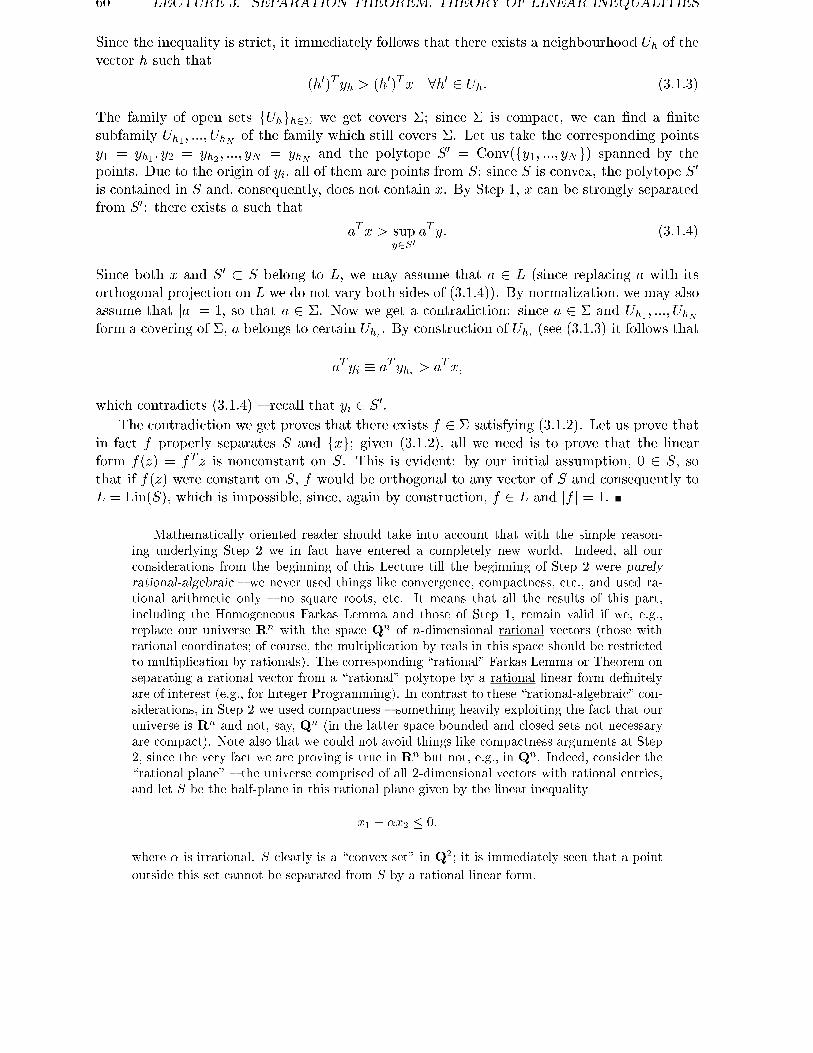
60 LECTURE 3. SEPARATION THEOREM. THEORY OF LINEAR INEQUALITIES
Since the inequality is strict, it immediately follows that there exists a neighbourhood Uh of thevector h such that
(h0)T yh > (h0)Tx 8h0 2 Uh: (3.1.3)
The family of open sets fUhgh2� we get covers �; since � is compact, we can �nd a �nitesubfamily Uh1 ; :::; UhN of the family which still covers �. Let us take the corresponding pointsy1 = yh1 ; y2 = yh2 ; :::; yN = yhN and the polytope S0 = Conv(fy1; :::; yNg) spanned by thepoints. Due to the origin of yi, all of them are points from S; since S is convex, the polytope S0
is contained in S and, consequently, does not contain x. By Step 1, x can be strongly separatedfrom S0: there exists a such that
aTx > supy2S0
aT y: (3.1.4)
Since both x and S0 � S belong to L, we may assume that a 2 L (since replacing a with itsorthogonal projection on L we do not vary both sides of (3.1.4)). By normalization, we may alsoassume that jaj = 1, so that a 2 �. Now we get a contradiction: since a 2 � and Uh1 ; :::; UhNform a covering of �, a belongs to certain Uhi . By construction of Uhi (see (3.1.3) it follows that
aT yi � aT yhi > aTx;
which contradicts (3.1.4) { recall that yi 2 S0.The contradiction we get proves that there exists f 2 � satisfying (3.1.2). Let us prove that
in fact f properly separates S and fxg; given (3.1.2), all we need is to prove that the linearform f(z) = fT z is nonconstant on S. This is evident: by our initial assumption, 0 2 S, sothat if f(z) were constant on S, f would be orthogonal to any vector of S and consequently toL = Lin(S), which is impossible, since, again by construction, f 2 L and jf j = 1.
Mathematically oriented reader should take into account that with the simple reason-ing underlying Step 2 we in fact have entered a completely new world. Indeed, all ourconsiderations from the beginning of this Lecture till the beginning of Step 2 were purelyrational-algebraic { we never used things like convergence, compactness, etc., and used ra-tional arithmetic only { no square roots, etc. It means that all the results of this part,including the Homogeneous Farkas Lemma and those of Step 1, remain valid if we, e.g.,replace our universe Rn with the space Qn of n-dimensional rational vectors (those withrational coordinates; of course, the multiplication by reals in this space should be restrictedto multiplication by rationals). The corresponding \rational" Farkas Lemma or Theorem onseparating a rational vector from a \rational" polytope by a rational linear form de�nitelyare of interest (e.g., for Integer Programming). In contrast to these \rational-algebraic" con-siderations, in Step 2 we used compactness { something heavily exploiting the fact that ouruniverse is Rn and not, say, Qn (in the latter space bounded and closed sets not necessaryare compact). Note also that we could not avoid things like compactness arguments at Step2, since the very fact we are proving is true in Rn but not, e.g., in Qn. Indeed, consider the\rational plane" { the universe comprised of all 2-dimensional vectors with rational entries,and let S be the half-plane in this rational plane given by the linear inequality
x1 + �x2 � 0;
where � is irrational. S clearly is a \convex set" in Q2; it is immediately seen that a point
outside this set cannot be separated from S by a rational linear form.

3.1. THE SEPARATION THEOREM 61
Step 3. Separation of two nonempty and non-intersecting convex sets. Now we areready to prove that two nonempty and non-intersecting convex sets S and T can be properlyseparated. To this end consider the arithmetic di�erence
� = S � T = fx� y j x 2 S; y 2 Tg:
We know from Proposition 2.1.5 that � is convex (and, of course, nonempty) set; since S and Tdo not intersect, � does not contain 0. By Step 2, we can properly separate � and f0g: thereexists h such that
fT0 = 0 � supz2�
fT z & fT0 > infz2�
fT z:
In other words,0 � sup
x2S;y2T[fTx� fTy] & 0 > inf
x2S;y2T[fTx� fT y];
which clearly means that f properly separates S and T .
Step 4. Separation of nonempty convex sets with non-intersecting relative interiors.Now we are able to complete the proof of the \if" part of the Separation Theorem. Let S andT be two nonempty convex sets with non-intersecting relative interiors; we should prove that Sand T can be properly separated. This is immediate: as we know from Theorem 2.1.1, the setsS0 = riS and T 0 = riT are nonempty and convex; since we are given that they do not intersect,they can be properly separated by Step 3: there exists f such that
infx2T 0
fTx � supy2S0
fTx & supx2T 0
fTx > infy2S0
fTx: (3.1.5)
It is immediately seen that in fact f properly separates S and T . Indeed, the quantities in theleft and the right hand sides of the �rst inequality in (3.1.5) clearly remain unchanged when wereplace S0 with clS0 and T 0 with clT 0; by Theorem 2.1.1, clS0 = clS � S and clT 0 = clT � T ,and we get infx2T fTx = infx2T 0 f
Tx, and similarly supy2S fT y = supy2S0 f
T y. Thus, we getfrom (3.1.5)
infx2T
fTx � supy2S
fT y:
It remains to note that T 0 � T , S0 � S, so that the second inequality in (3.1.5) implies that
supx2T
fTx > infy2S
fTx:
3.1.3 Strong separation
We know from the Separation Theorem what are simple necessary and suÆcient conditionsfor proper separation of two convex sets - their relative interiors should be disjoint. There isalso a simple necessary and suÆcient condition for two sets to be strongly separated:
Proposition 3.1.1�Two nonempty convex sets S and T in Rn can be strongly separated
if and only if these sets are "at positive distance":
�(S; T ) = infx2S;y2T
jx� yj > 0:
This, is, in particular, the case when one of the sets is compact, the other one is closed andthe sets do not intersect.

62 LECTURE 3. SEPARATION THEOREM. THEORY OF LINEAR INEQUALITIES
Proof�. The necessity - the "only if" part - is evident: if S and T can be properly separated,
i.e., for certain a one has� � sup
x2SaTx < � � inf
y2TaT y;
then for every pair (x; y) with x 2 S and y 2 T one has
jx� yj � � � �
jaj(since otherwise we would get from Cauchy's inequality (1.1.2)
aT y � aTx = aT (y � x) � jajjy � xj < � � �;
which is impossible).To prove the suÆciency - the "if" part - consider the set � = S�T . This is a convex set
which clearly does not contain vectors of the length less than �(S; T ) > 0; consequently, itdoes not intersect the ball B of some positive radius r centered at the origin. Consequently,by the Separation Theorem Q can be properly separated from B: there exists a such that
infz2B
aT z � supx2S;y2T
fT (x� y) & supz2B
aT z > infx2S;y2T
fT (x� y): (3.1.6)
From the second of these inequalities it follows that a 6= 0 (as it always is the case withproper separation); therefore infz2B aT z < 0, so that the �rst inequality in (3.1.6) meansthat a strongly separates S and T .
The \in particular" part of the statement is a simple exercise from Analysis: two closed
nonempty and non-intersecting subsets ofRn with one of them being compact are at positive
distance from each other.
3.2 Theory of �nite systems of linear inequalities
The Separation Theorem and the main tool we have developed when proving it { the Homoge-neous Farkas Lemma { are the most useful and most frequently used results of Convex Analysis;it will be clearly seen from our forthcoming lectures. Right now we shall use the Farkas Lemmato get one of the deepest results of the theory of (�nite) systems of linear inequalities { theGeneral Theorem on Alternative. The question we are interested in is as follows.
An arbitrary �nite system of linear inequalities can be written down as
(I)Sx < pNx � q
where x 2 Rn is the vector of unknowns, S ("Strict") and N ("Non-strict") are �xed matricesof the column size n and certain row sizes, and p; q are �xed vectors of appropriate dimensions.Note that we may include into consideration linear equalities as well, representing every equalityof this type by a pair of opposite nonstrict inequalities.
The main question related to system (I) is whether or not the system is solvable. If we knowhow to answer such a question, we also know how to answer many other questions, e.g.
� whether a given linear inequality aTx<�=b is a consequence of (I), i.e., is satis�ed at all
solutions to the system
(indeed, an inequality is a consequence of (I) if and only if the system comprised of (I)and the negation of this inequality has no solutions),
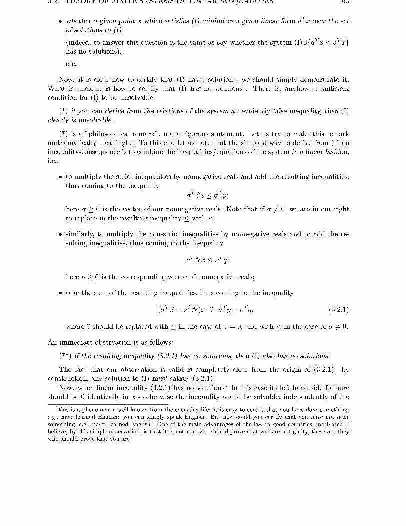
3.2. THEORY OF FINITE SYSTEMS OF LINEAR INEQUALITIES 63
� whether a given point �x which satis�es (I) minimizes a given linear form aTx over the setof solutions to (I)
(indeed, to answer this question is the same as say whether the system (I)[faTx < aT �xghas no solutions),
etc.
Now, it is clear how to certify that (I) has a solution - we should simply demonstrate it.What is unclear, is how to certify that (I) has no solutions1. There is, anyhow, a suÆcientcondition for (I) to be unsolvable:
(*) if you can derive from the relations of the system an evidently false inequality, then (I)clearly is unsolvable.
(*) is a "philosophical remark", not a rigorous statement. Let us try to make this remarkmathematically meaningful. To this end let us note that the simplest way to derive from (I) aninequality-consequence is to combine the inequalities/equations of the system in a linear fashion,i.e.,
� to multiply the strict inequalities by nonnegative reals and add the resulting inequalities,thus coming to the inequality
�TSx � �T p;
here � � 0 is the vector of our nonnegative reals. Note that if � 6= 0, we are in our rightto replace in the resulting inequality � with <;
� similarly, to multiply the non-strict inequalities by nonnegative reals and to add the re-sulting inequalities, thus coming to the inequality
�TNx � �T q;
here � � 0 is the corresponding vector of nonnegative reals;
� take the sum of the resulting inequalities, thus coming to the inequality
(�TS + �TN)x ? �T p+ �T q; (3.2.1)
where ? should be replaced with � in the case of � = 0, and with < in the case of � 6= 0.
An immediate observation is as follows:
(**) if the resulting inequality (3.2.1) has no solutions, then (I) also has no solutions.
The fact that our observation is valid is completely clear from the origin of (3.2.1): byconstruction, any solution to (I) must satisfy (3.2.1).
Now, when linear inequality (3.2.1) has no solutions? In this case its left hand side for sureshould be 0 identically in x - otherwise the inequality would be solvable, independently of the
1this is a phenomenon well-known from the everyday life: it is easy to certify that you have done something,e.g., have learned English: you can simply speak English. But how could you certify that you have not donesomething, e.g., never learned English? One of the main advantages of the law in good countries, motivated, Ibelieve, by this simple observation, is that it is not you who should prove that you are not guilty, these are theywho should prove that you are

64 LECTURE 3. SEPARATION THEOREM. THEORY OF LINEAR INEQUALITIES
value of the right hand side. Thus, we should have [�TS + �TN ]x = 0 for all x, or, which is thesame, should have
ST� +NT � = 0:
Our further conclusions depend on whether � = 0 { then the sign in the inequality is �, andit has no solutions if the right hand side is strictly negative { or � 6= 0; in this latter case thesign in the inequality is <, and it has no solutions if its right hand side is nonpositive. Thus,we have established the following principle:
To certify that (I) has no solutions, it is suÆcient to demonstrate that the following conditionholds:
(!): There exist vectors
� � 0; � � 0
of the dimensions equal to the # of rows in S and N , respectively, such that
ST� +NT � = 0;
and, in addition,
� in the case of � 6= 0: �T p+ �T q � 0;
� in the case of � = 0: �T q < 0.
A crucial for the theory of linear inequalities fact is that the condition (!) is not onlysuÆcient, as we just have seen, but also necessary for inconsistency of (I):
Theorem 3.2.1 [General Theorem on Alternative] Condition (!) is necessary and suÆcientcondition for (I) to have no solutions.
We shall prove the \necessity" part of this theorem (the \suÆciency" part is already proved) inthe end of this section. Right now let me make several remarks.
� the main advantage of Theorem 3.2.1 is that it reformulates certain negative statement- \(I) has no solutions" - as a positive statement: existence of certain vectors � and �satisfying a number of explicit and veri�able relations. This is why this theorem is the keyto numerous useful results, e.g., to the Duality Theorem for Linear Programming
� there are many corollaries, or, better to say, particular cases of Theorem 3.2.1 (we shalllist some of these corollaries below). All these cases are obtained by the straightforwardspeci�cation of condition (!) for the particular form of the data in (I) in the case in question.I do not think that you should learn \by heart" all particular forms of the Theorem; itis much easier to remember properly what is the actual meaning of the Theorem - \asystem of linear inequalities has no solution if and only if combining, in the linear fashion,the inequalities from the system one can obtain a contradictory inequality" { and to look(this is always quite straightforward) what this "receipt" means in the particular case inquestion
� the most important - the \necessity" - part of Theorem 3.2.1 heavily depends on thefact that the system (I) in question is comprised of linear inequalities. Unfortunately, its

3.2. THEORY OF FINITE SYSTEMS OF LINEAR INEQUALITIES 65
natural extension to the case of more general inequalities, say, the quadratic ones, fails tobe true. E.g, the system of quadratic equalities
x2 � 1; y2 � 1; �(x+ y)2 � �5with two unknowns x and y clearly has no solution; there is no, anyhow, a combination ofthese inequalities with nonnegative coeÆcients which is "evidently contradictory", i.e., isof the form 0 � �1. This is actually a disaster - in fact this is the reason for existence ofcomplicated combinatorial problems for which no eÆcient solution algorithms are known
Now let us formulate some particular cases of Theorem 3.2.1 which are often used; it is a goodexercise to derive these corollaries from the General Theorem on Alternative.
The �rst particular case is the Gordan Theorem on Alternative:
Theorem 3.2.2 [Gordan's Theorem on Alternative] One of the inequality systems
(I) Ax < 0; x 2 Rn;
(II) AT y = 0; 0 6= y � 0; y 2 Rm;
A being an m� n matrix, has a solution if and only if the other one has no solutions.
The second particular case is the Homogeneous Farkas Lemma which we already know. In ournew (clearly equivalent to the original one) form it sounds as follows:
Theorem 3.2.3 [The Homogeneous Farkas Lemma] A homogeneous linear inequality
aTx � 0 (3.2.2)
is a consequence of a system of linear homogeneous inequalities
Nx � 0 (3.2.3)
if and only ifa = AT �
for some nonnegative vector �.
Note that the implication \Theorem 3.2.1) Homogeneous Farkas Lemma" is of no actual value{ we still did not prove the necessity part of the Theorem; in fact our proof will be based exactlyon the Homogeneous Farkas Lemma which we already have proven.
The next particular case is
Theorem 3.2.4 [Inhomogeneous Farkas Lemma] A linear inequality
aTx � p (3.2.4)
is a consequence of a solvable system of linear inequalities
Nx � q (3.2.5)
if and only if it is a "linear consequence" of the system and the trivial inequality
0Tx � 1;

66 LECTURE 3. SEPARATION THEOREM. THEORY OF LINEAR INEQUALITIES
i.e., if it can be obtained by taking weighted sum, with nonnegative coeÆcients, of the inequalitiesfrom the system and this trivial inequality.
Algebraically: (3.2.4) is a consequence of solvable system (3.2.5) if and only if
a = NT �
for some nonnegative vector � such that
�T q � p:
The last example is
Theorem 3.2.5 [Motzkin's Theorem on Alternative] The system
Sx < 0; Nx � 0
has no solutions if and only if the system
ST� +NT � = 0; � � 0; � � 0; � 6= 0
has a solution.
3.2.1 Proof of the "necessity" part of the Theorem on Alternative
We shall derive the desired statement from the Homogeneous Farkas Lemma. The situationis as follows: we know that the system
(I)Sx < pNx � q
has no solutions, and we should prove the existence of � and � required by (!).To this end let us extend our space of variables x by three variables, u; v and t, and
consider the following system of homogeneous nonstrict inequalities:
(I0)
Sx+ ue� vp � 0Nx� vq � 0�u+ t � 0�v + t � 0
;
e being the vector of ones of the dimension equal to the row dimension of S.We claim that (I0) implies the linear homogeneous inequality
(I00) t � 0:
Indeed, if there were a solution (x; u; v; t) to (I0) with t > 0, we would have from the last twoinequalities of (I0) u � t > 0, v � t > 0; then the �rst two inequalities in (I0) would imply
Sx
v� p� u
ve < p; N
x
v� q;
i.e., (I) would be solvable, which is assumed not to be the case.Thus, (I0) implies (I00). By the Homogeneous Farkas Lemma, there exist nonnegative
vectors �, � and nonnegative reals �; � such that the vector of coeÆcients in the left handside of the inequality (I00), i.e. the vector 0B@
0x0u0v1t
1CA
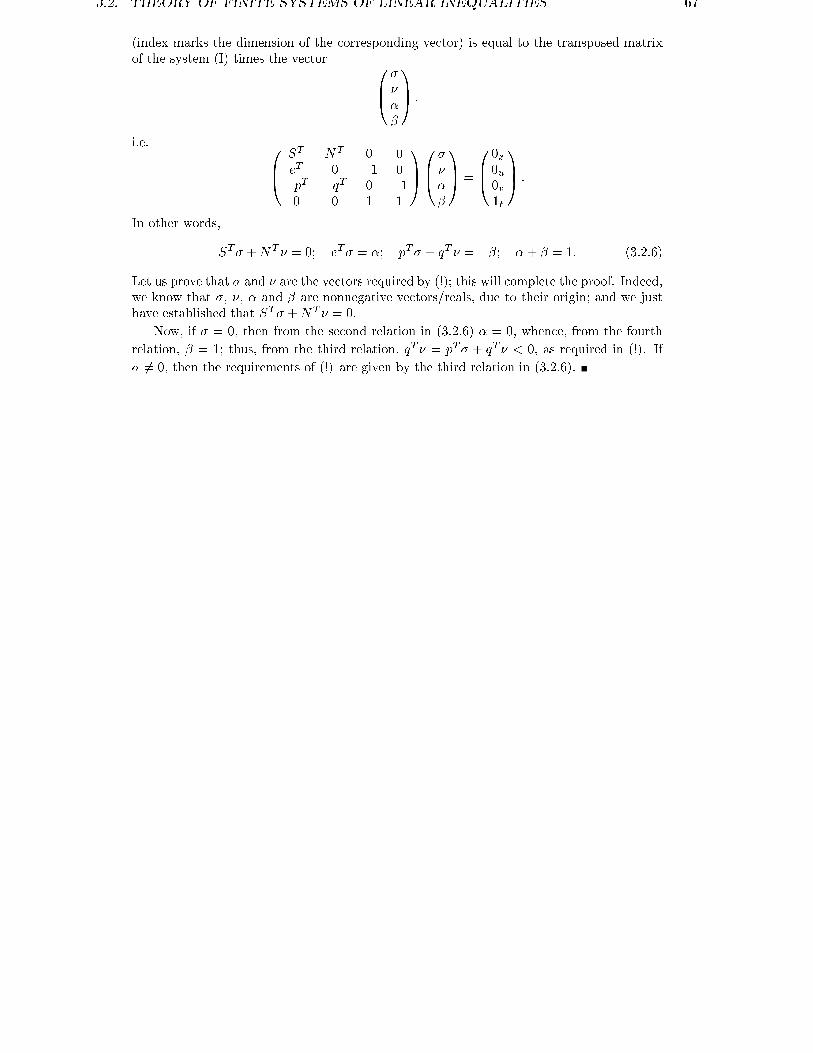
3.2. THEORY OF FINITE SYSTEMS OF LINEAR INEQUALITIES 67
(index marks the dimension of the corresponding vector) is equal to the transposed matrixof the system (I) times the vector 0B@
����
1CA ;
i.e. 0B@ST NT 0 0eT 0 �1 0�pT �qT 0 �10 0 1 1
1CA0B@����
1CA =
0B@0x0u0v1t
1CA :
In other words,
ST� +NT � = 0; eT� = �; pT� + qT � = ��; �+ � = 1: (3.2.6)
Let us prove that � and � are the vectors required by (!); this will complete the proof. Indeed,we know that �, �, � and � are nonnegative vectors/reals, due to their origin; and we justhave established that ST� +NT � = 0.
Now, if � = 0, then from the second relation in (3.2.6) � = 0, whence, from the fourth
relation, � = 1; thus, from the third relation, qT � = pT� + qT � < 0, as required in (!). If
� 6= 0, then the requirements of (!) are given by the third relation in (3.2.6).

68 LECTURE 3. SEPARATION THEOREM. THEORY OF LINEAR INEQUALITIES
Assignment # 3 (Lecture 3)
Exercise 3.1 Which of the following pairs (S; T ) of sets are (a) properly separated and (b)strongly separated by the linear form f(x) = x1:
� S = fx 2 Rn j Pni=1 x
2i � 1g, T = fx 2 Rn j x1 + x2 � 2; x1 � x2 � 0g;
� S = fx 2 Rn j Pni=1 x
2i � 1g, T = fx 2 Rn j x1 + x2 � 2; x1 � x2 � �1g;
� S = fx 2 Rn j Pni=1 jxij � 1g, T = fx 2 Rn j x1 + x2 � 2; x1 � x2 � 0g;
� S = fx 2 Rn j maxi=1;:::;n xi � 1g, T = fx 2 Rn j x1 + x2 � 2; x1 � x2 � �1g;
� S = fx 2 Rn j x1 = 0g, T = fx 2 Rn j x1 �qx22 + :::+ x2ng;
� S = fx 2 Rn j x1 = 0g, T = fx 2 Rn j x1 = 1g;� S = fx 2 Rn j x1 = 0; x22 + :::+ x2n � 1g, T = fx 2 Rn j x1 = 0; x2 � 100g;� S = fx 2 R2 j x1 > 0; x2 � 1=x1g, T = fx 2 R2 j x1 < 0; x2 � �1=x1g.
Do at least 2, on your choice, of the following 3 exercises 3.2 - 3.4:
Exercise 3.2 Derive Gordan's Theorem on Alternative (Theorem 3.2.2) from the General The-orem on Alternative
Exercise 3.3 Derive Inhomogeneous Farkas Lemma (Theorem 3.2.4) from the General Theo-rem on Alternative
Exercise 3.4 Derive Motzkin's Theorem on Alternative (Theorem 3.2.5) from the General The-orem on Alternative
Exercise 3.5 Which of the following systems of linear inequalities with 2 unknowns have, andwhich have no solutions (for the systems which are solvable, point out a solution; for the unsolv-able systems, explain why they are so):
�8<:x+ y � 22x� y � 1�5x+ y � �5
�8<:x+ y � 22x� y � 1�5x+ y � �4
�8<:x+ y � 22x� y � 1�5x+ y � �3:5
Exercise 3.6 Consider the linear inequality
x+ y � 2

3.2. THEORY OF FINITE SYSTEMS OF LINEAR INEQUALITIES 69
and the system of linear inequalities �x � 1�x � �100
Our inequality clearly is a consequence of the system { it is satis�ed at every solution to it (simplybecause there are no solutions to the system at all). According to the Inhomogeneous FarkasLemma, the inequality should be a linear consequence of the system and the trivial inequality0 � 1, i.e., there should exist nonnegative �1; �2 such that�
11
�= �1
�10
�+ �2
��10
�; �1 � 1000�2 � 2;
which clearly is not the case. What is the reason for the observed \contradiction"?
Optional exercises
Exercise 3.7 Prove the following fact:
Let S be a nonempty and closed convex set in Rn, and let T = fxg be a singletonoutside S (x 62 S). Consider the optimization program
minfjx� yj j y 2 Sg:
The program is solvable and has a unique solution y�, and the linear form aTh,a = x� y�, strongly separates T and S:
supy2S
aT y = aT y� = aTx� jaj2:
Remark. The indicated statement is a key argument for an alternative proof of the SeparationTheorem. It is an excellent exercise { to derive the Separation Theorem from the above fact.

70 LECTURE 3. SEPARATION THEOREM. THEORY OF LINEAR INEQUALITIES
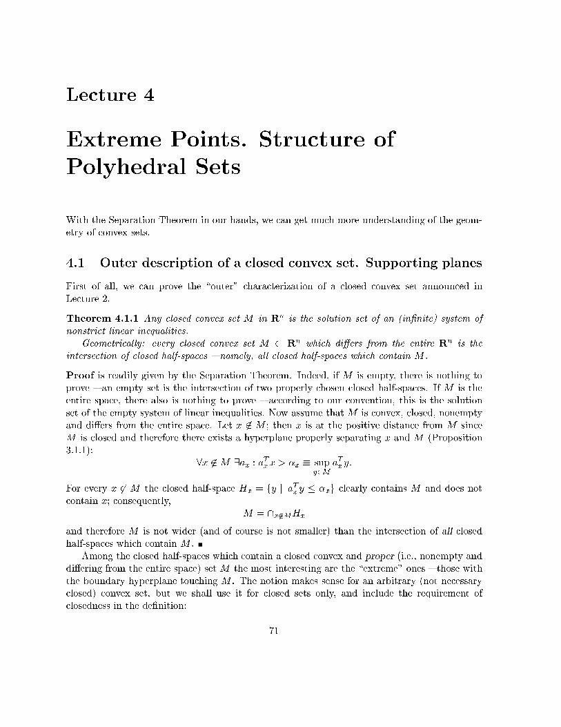
Lecture 4
Extreme Points. Structure ofPolyhedral Sets
With the Separation Theorem in our hands, we can get much more understanding of the geom-etry of convex sets.
4.1 Outer description of a closed convex set. Supporting planes
First of all, we can prove the \outer" characterization of a closed convex set announced inLecture 2.
Theorem 4.1.1 Any closed convex set M in Rn is the solution set of an (in�nite) system ofnonstrict linear inequalities.
Geometrically: every closed convex set M � Rn which di�ers from the entire Rn is theintersection of closed half-spaces { namely, all closed half-spaces which contain M .
Proof is readily given by the Separation Theorem. Indeed, if M is empty, there is nothing toprove { an empty set is the intersection of two properly chosen closed half-spaces. If M is theentire space, there also is nothing to prove { according to our convention, this is the solutionset of the empty system of linear inequalities. Now assume that M is convex, closed, nonemptyand di�ers from the entire space. Let x 62 M ; then x is at the positive distance from M sinceM is closed and therefore there exists a hyperplane properly separating x and M (Proposition3.1.1):
8x 62M 9ax : aTxx > �x � supy2M
aTx y:
For every x 62 M the closed half-space Hx = fy j aTx y � �xg clearly contains M and does notcontain x; consequently,
M = \x62MHx
and therefore M is not wider (and of course is not smaller) than the intersection of all closedhalf-spaces which contain M .
Among the closed half-spaces which contain a closed convex and proper (i.e., nonempty anddi�ering from the entire space) set M the most interesting are the \extreme" ones { those withthe boundary hyperplane touching M . The notion makes sense for an arbitrary (not necessaryclosed) convex set, but we shall use it for closed sets only, and include the requirement ofclosedness in the de�nition:
71

72 LECTURE 4. EXTREME POINTS. STRUCTURE OF POLYHEDRAL SETS
De�nition 4.1.1 [Supporting plane] Let M be a convex closed set in Rn, and let x be a pointfrom the relative boundary of M . A hyperplane
� = fy j aT y = aTxg [a 6= 0]
is called supporting to M at x, if it properly separates M and fxg, i.e., ifaTx � sup
y2MaT y & aTx > inf
y2MaT y: (4.1.1)
Note that since x is a point from the relative boundary ofM and therefore belongs to clM =M ,the �rst inequality in (4.1.1) in fact is equality. Thus, an equivalent de�nition of a supportingplane is as follows:
Let M be a closed convex set and x be a relative boundary point of M . Thehyperplane fy j aT y = aTxg is called supporting to M at x, if the linear forma(y) = aT y attains its maximum on M at the point x and is nonconstant on M .
E.g., the hyperplane fx1 = 1g inRn clearly is supporting to the unit Euclidean ball fx j jxj � 1gat the point x = e1 = (1; 0; :::; 0).
The most important property of a supporting plane is its existence:
Proposition 4.1.1 [Existence of supporting hyperplane] Let M be a convex closed set in Rn
and x be a point from the relative boundary of M . Then(i) There exists at least one hyperplane which is supporting to M at x;(ii) If � is supporting to M at x, then the intersection M \� is of aÆne dimension less than
the one of M (recall that the aÆne dimension of a set is, by de�nition, the aÆne dimension ofthe aÆne hull of the set).
Proof. (i) is easy: if x is a point from the relative boundary ofM , then it is outside the relativeinterior ofM and therefore fxg and riM can be properly separated by the Separation Theorem;the separating hyperplane is exactly the desired supporting to M at x hyperplane.
To prove (ii), note that if � = fy j aT y = aTxg is supporting to M at x 2 @riM , then theset M 0 = M \ � is nonempty (it contains x) convex set, and the linear form aT y is constanton M 0 and therefore (why?) on A�(M 0). At the same time, the form is nonconstant on M byde�nition of a supporting plane. Thus, A�(M 0) is a proper (less than the entire A�(M)) subsetof A�(M), and therefore the aÆne dimension of A�(M 0) (i.e., the aÆne dimension of M 0) isless than the aÆne dimension of A�(M) (i.e., than the aÆne dimension of M). 1).
4.2 Minimal representation of convex sets: extreme points
Supporting planes are useful tool to prove existence of extreme points of convex sets. Geometri-cally, an extreme point of a convex set M is a point inM which cannot be obtained as a convexcombination of other points of the set; and the importance of the notion comes from the fact(which we shall prove in the mean time) that the set of all extreme points of a \good enough"convex set M is the \shortest worker's instruction for building the set" { this is the smallest setof points for which M is the convex hull.
The exact de�nition of an extreme point is as follows:1) In the latter reasoning we used the following fact: if P � Q are two aÆne sets, then the aÆne dimension of
P is � the one of Q, with � being = if and only if P = Q. We know similar statement for linear subspaces (seeLecture 1); please prove (it is immediate) that it is valid for aÆne sets as well

4.2. MINIMAL REPRESENTATION OF CONVEX SETS: EXTREME POINTS 73
De�nition 4.2.1 [extreme points] Let M be a nonempty convex set in Rn. A point x 2 M iscalled an extreme point of M , if there is no nontrivial (of positive length) segment [u; v] 2 Mfor which x is an interior point, i.e., if the relation
x = �u+ (1� �)v
with certain � 2 (0; 1) and u; v 2M is possible if and only if
u = v = x:
E.g., the extreme points of a segment are exactly its endpoints; the extreme points of a triangleare its vertices; the extreme points of a (closed) circle on the 2-dimensional plane are the pointsof the circumference.
An equivalent de�nition of an extreme point is as follows:
Proposition 4.2.1+A point x in a convex set M is extreme if and only if the set Mnfxg is
convex.
It is clear that a convex set M not necessarily possesses extreme points; as an example you maytake the open unit ball in Rn. This example is not interesting { the set in question is not closed;when replacing it with its closure, we get a set (the closed unit ball) with plenty of extremepoints { these are all points of the boundary. There are, however, closed convex sets which donot possess extreme points { e.g., a line or an aÆne set of larger dimension. A nice fact is thatthe absence of extreme points in a closed convex set M always has the standard reason { theset contains a line. Thus, a closed and nonempty convex set M which does not contain linesfor sure possesses extreme points. And if M is nonempty convex compact, it possesses a quiterepresentative set of extreme points { their convex hull is the entire M . Namely, we have thefollowing
Theorem 4.2.1 Let M be a closed and nonempty convex set in Rn. Then(i) The set Ext(M) of extreme points of M is nonempty if and only if M does not contain
lines;(ii) If M is bounded, then M is the convex hull of its extreme points:
M = Conv(Ext(M));
so that every point of M is a convex combination of the points of Ext(M).
Note that part (ii) of this theorem is the �nite-dimensional version of the famous Krein-MilmanTheorem.Proof. Let us start with (i). The "only if" part is easy, due to the following simple
Lemma 4.2.1 LetM be a closed convex set in Rn. Assume that for some �x 2Mand h 2 Rn M contains the ray
f�x+ th j t � 0gstarting at �x with the direction h. Then M contains also all parallel rays starting atthe points of M :
(8x 2M) : fx+ th j t � 0g �M:
In particular, ifM contains certain line, then it contains also all parallel lines passingthrough the points of M .

74 LECTURE 4. EXTREME POINTS. STRUCTURE OF POLYHEDRAL SETS
Comment. For a convex set M; the set of all directions h such that x + th 2 Mfor some x and all t � 0 (i.e., by Lemma { such that x+ th 2M for all x 2M andall t � 0) is called the recessive cone of M [notation: Rec(M)]. With Lemma 4.2.1it is immediately seen (prove it!) that Rec(M) indeed is a cone, and that
M +Rec(M) =M:
Directions from Rec(M) are called recessive for M .
Proof of the lemma is immediate: if x 2 M and �x + th 2 M for all t � 0, then,due to convexity, for any �xed � � 0 we have
�(�x+�
�h) + (1� �)x 2M
for all � 2 (0; 1). As � ! +0, the left hand side tends to x + �h, and since M isclosed, x+ �h 2M for every � � 0.
Lemma 4.2.1, of course, resolves all our problems with the "only if" part. Indeed, here weshould prove that if M possesses extreme points, then M does not contain lines, or, which isthe same, that if M contains lines, then it has no extreme points. But the latter statement isimmediate: if M contains a line, then, by Lemma, there is a line in M passing through anygiven point of M , so that no point can be extreme.
Now let us prove the "if" part of (i). Thus, from now on we assume that M does not containlines; our goal is to prove that then M possesses extreme points. Let us start with the following
Lemma 4.2.2 Let Q be a nonempty closed convex set, �x be a relative boundarypoint of Q and � be a hyperplane supporting to Q at �x. Then all extreme points ofthe nonempty closed convex set � \Q are extreme points of Q.
Proof of the Lemma. First, the set �\Q is closed and convex (as an intersec-tion of two sets with these properties); it is nonempty, since it contains �x (� contains�x due to the de�nition of a supporting plane, and Q contains �x due to the closednessof Q). Second, let a be the linear form associated with �:
� = fy j aT y = aT �xg;so that
infx2Q
aTx < supx2Q
aTx = aT �x (4.2.1)
(see Proposition 4.1.1). Assume that y is an extreme point of �\Q; what we shoulddo is to prove that y is an extreme point of Q, or, which is the same, to prove that
y = �u+ (1� �)v
for some u; v 2 Q and � 2 (0; 1) is possible only if y = u = v. To this end it suÆcesto demonstrate that under the above assumptions u; v 2 � \ Q (or, which is thesame, to prove that u; v 2 �, since the points are known to belong to Q); indeed,we know that y is an extreme point of �\Q, so that the relation y = �u+ (1� �)vwith � 2 (0; 1) and u; v 2 � \Q does imply y = u = v.
To prove that u; v 2 �, note that since y 2 � we have
aT y = aT �x � maxfaTu; aT vg

4.2. MINIMAL REPRESENTATION OF CONVEX SETS: EXTREME POINTS 75
(the concluding inequality follows from (4.2.1)). On the other hand,
aT y = �aTu+ (1� �)aT v;
combining these observations and taking into account that � 2 (0; 1), we concludethat
aT y = aTu = aT v:
But these equalities imply that u; v 2 �.
Equipped with the Lemma, we can easily prove (i) by induction on the dimension of theconvex set M (recall that this is nothing but the aÆne dimension of the aÆne span of M , i.e.,the linear dimension of the linear subspace L such that A�(M) = a+ L).
There is nothing to do if the dimension of M is zero, i.e., if M is a point - then, of course,M = Ext(M). Now assume that we already have proved the nonemptiness of Ext(T ) for allnonempty closed and not containing lines convex sets T of certain dimension k, and let us provethat the same statement is valid for the sets of dimension k + 1. Let M be a closed convexnonempty and not containing lines set of dimension k + 1. Since M does not contain lines andis of positive dimension, it di�ers from A�(M) and therefore it possesses a relative boundarypoint �x 2). According to Proposition 4.1.1, there exists a hyperplane � = fx j aTx = aT �xgwhich supports M at �x:
infx2M
aTx < maxx2M
aTx = aT �x:
By the same Proposition, the set T = � \M (which is closed, convex and nonempty) is ofaÆne dimension less than the one of M , i.e., of the dimension � k. T clearly does not containlines (since even the larger set M does not contain lines). By Inductive Hypothesis, T possessesextreme points, and by Lemma 4.2.2 all these points are extreme also forM . The inductive stepis complete, and (i) is proved.
Now let us prove (ii). Thus, let M be nonempty, convex, closed and bounded; we shouldprove that
M = Conv(Ext(M)):
What is immediately seen is that the right hand side set is contained in the left hand side one.Thus, all we need is to prove that any x 2 M is a convex combination of points from Ext(M).Here we again use induction on the dimension of M . The case of 0-dimensional set M (i.e., apoint) is trivial. Assume that the statement in question is valid for all k-dimensional convexclosed and bounded sets, and let M be a convex closed and bounded set of dimension k+1. Letx 2M ; to represent x as a convex combination of points from Ext(M), let us pass through x anarbitrary line l = fx + �h j � 2 Rg (h 6= 0) in the aÆne span A�(M). Moving along this linefrom x in each of the two possible directions, we eventually leave M (since M is bounded); as
2)Indeed, there exists z 2 A�(M)nM , so that the points
x� = x+ �(z � x)
(x is an arbitrary �xed point of M) do not belong to M for some � � 1, while x0 = x belongs to M . The set ofthose � � 0 for which x� 2M is therefore nonempty and bounded from above; this set clearly is closed (since Mis closed). Thus, there exists the largest � = �� for which x� 2 M . We claim that x�� is a relative boundarypoint of M . Indeed, by construction this is a point fromM . If it would be a point from the relative interior of M ,then all the points x� with close to �� and greater than �� values of � would also belong to M , which contradictsthe origin of ��

76 LECTURE 4. EXTREME POINTS. STRUCTURE OF POLYHEDRAL SETS
it was explained in the proof of (i), it means that there exist nonnegative �+ and �� such thatthe points
�x� = x+ ��h
both belong to the relative boundary of M . Let us verify that �x� are convex combinations ofthe extreme points of M (this will complete the proof, since x clearly is a convex combinationof the two points �x�). Indeed, M admits supporting at �x+ hyperplane �; as it was explained inthe proof of (i), the set �\M (which clearly is convex, closed and bounded) is of less dimensionthan that one ofM ; by the inductive hypothesis, the point �x+ of this set is a convex combinationof extreme points of the set, and by Lemma 4.2.2 all these extreme points are extreme pointsof M as well. Thus, �x+ is a convex combination of extreme points of M . Similar reasoning isvalid for �x�.
4.3 Structure of polyhedral sets
As the �rst fruits of our developments, we are about to establish an extremely important resulton the structure of a polyhedral set. (which, in turn, will immediately imply basically all theoryof Linear Programming).
According to our de�nition (Lecture 2), a polyhedral set M is the set of all solutions to a�nite system of nonstrict linear inequalities:
M = fx 2 Rn j Ax � bg; (4.3.1)
A being a matrix of the column size n and certain row size m and b beingm-dimensional vector.This is the outer (\artist's") description of a polyhedral set; and what is the inner (\worker's")one?
To come to the answer, consider the following construction. Let us take two �nite nonemptyset of vectors V (\vertices") and R (\rays") and build the set
M(V;R) = Conv(V ) + Cone (R) = fXv2V
�vv +Xr2R
�rr j �v � 0; �r � 0;Xv
�v = 1g:
Thus, we take all vectors which can be represented as sums of convex combinations of the pointsfrom V and conic combinations of the points from R. The set M(V;R) clearly is convex (as thearithmetic sum of two convex sets Conv(V ) and Cone (R)). The promised inner description ofthe structure of polyhedral sets is as follows:
Theorem 4.3.1 [Structure of polyhedral set] The sets of the form M(V;R) are exactly thenonempty polyhedral sets: M(V;R) is polyhedral, and every nonempty polyhedral set M isM(V;R) for properly chosen V and R.
The polytopes M(V; f0g) = Conv(V ) are exactly the nonempty and bounded polyhedral sets.The sets of the type M(f0g; R) are exactly the polyhedral cones (sets given by �nitely manynonstrict homogeneous linear inequalities).
Remark 4.3.1 In addition to the results of the Theorem, it can be proved (we will not do itto save time) that in the representation of a nonempty polyhedral set M as M = Conv(V ) +Cone (R)
{ the \conic" part Conv(R) (not the set R itself!) is uniquely de�ned by M and is therecessive cone of M (see the Comment to Lemma 4.2.1);
{ if M does not contain lines, then V can be chosen as the set of all extreme points of M .

4.3. STRUCTURE OF POLYHEDRAL SETS 77
We postpone the proof of the Theorem till the end of the lecture; right now let me explain whythis theorem is that important { why it is so nice to know both inner and outer descriptions ofa polyhedral set.
Let us pose several natural questions:
� A. Is it true that the inverse image of a polyhedral set M � Rn under an aÆne mappingy 7! P(y) = Py + p : Rm ! Rn, i.e., the set
P�1(M) = fy 2 Rm j Py + p 2Mgis polyhedral?
� B. Is it true that the image of a polyhedral set M � Rn under an aÆne mapping x 7! y =P(x) = Px+ p : Rn ! Rm { the set
P(M) = fPx+ p j x 2Mgis polyhedral?
� C. Is it true that the intersection of two polyhedral sets is again a polyhedral set?
� D. Is it true that the arithmetic sum of two polyhedral sets is again a polyhedral set?
The answers to all these questions are, as we shall see, positive; what is very instructive is howthese positive answers are obtained.
It is very easy to answer aÆrmatively to A, starting from the original { outer { de�nition ofa polyhedral set: if M = fx j Ax � bg, then, of course,
P�1(M) = fy j A(Py + p) � bg = fy j (AP )y � b�Apgand therefore P�1(M) is a polyhedral set.
An attempt to answer aÆrmatively to B via the same de�nition fails { there is not seen aneasy way to update the linear inequalities de�ning a polyhedral set into those de�ning its image,and it is absolutely unclear why the image indeed is given by �nitely many linear inequalities.Note, however, that there is no diÆculty to answer aÆrmatively to B with the inner descriptionof a nonempty polyhedral set: if M =M(V;R), then, evidently,
P(M) =M(P(V ); PR);where PR = fPr j r 2 Rg is the image of R under the action of the homogeneous part of P.
Similarly, positive answer to C becomes evident, when we use the outer description of a poly-hedral set: taking intersection of the solution sets to two systems of nonstrict linear inequalities,we, of course, again get the solution set to a system of this type { you simply should put togetherall inequalities from the original two systems. And it is very unclear how to answer positively toD with the outer de�nition of a polyhedral set { what happens with inequalities when we addthe solution sets? In contrast to this, the inner description gives the answer immediately:
M(V;R) +M(V 0; R0) = Conv(V ) + Cone (R) + Conv(V 0) + Cone (R0)= [Conv(V ) + Conv(V 0)] + [Cone (R) + Cone (R0)]= Conv(V + V 0) + Cone (R [R0)= M(V + V 0; R [R0):
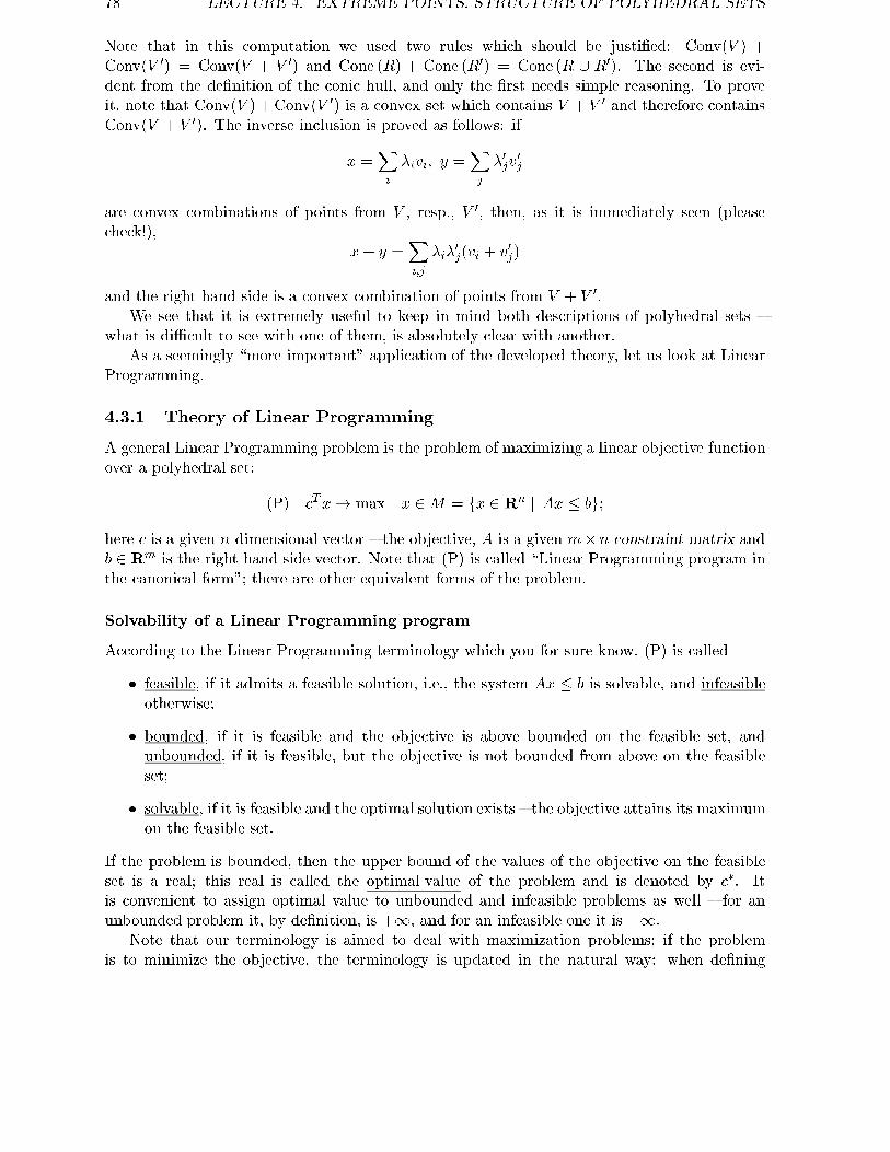
78 LECTURE 4. EXTREME POINTS. STRUCTURE OF POLYHEDRAL SETS
Note that in this computation we used two rules which should be justi�ed: Conv(V ) +Conv(V 0) = Conv(V + V 0) and Cone (R) + Cone (R0) = Cone (R [ R0). The second is evi-dent from the de�nition of the conic hull, and only the �rst needs simple reasoning. To proveit, note that Conv(V ) +Conv(V 0) is a convex set which contains V + V 0 and therefore containsConv(V + V 0). The inverse inclusion is proved as follows: if
x =Xi
�ivi; y =Xj
�0jv0j
are convex combinations of points from V , resp., V 0, then, as it is immediately seen (pleasecheck!),
x+ y =Xi;j
�i�0j(vi + v0j)
and the right hand side is a convex combination of points from V + V 0.We see that it is extremely useful to keep in mind both descriptions of polyhedral sets {
what is diÆcult to see with one of them, is absolutely clear with another.As a seemingly \more important" application of the developed theory, let us look at Linear
Programming.
4.3.1 Theory of Linear Programming
A general Linear Programming problem is the problem of maximizing a linear objective functionover a polyhedral set:
(P) cTx! max j x 2M = fx 2 Rn j Ax � bg;
here c is a given n-dimensional vector { the objective, A is a given m�n constraint matrix andb 2 Rm is the right hand side vector. Note that (P) is called \Linear Programming program inthe canonical form"; there are other equivalent forms of the problem.
Solvability of a Linear Programming program
According to the Linear Programming terminology which you for sure know, (P) is called
� feasible, if it admits a feasible solution, i.e., the system Ax � b is solvable, and infeasibleotherwise;
� bounded, if it is feasible and the objective is above bounded on the feasible set, andunbounded, if it is feasible, but the objective is not bounded from above on the feasibleset;
� solvable, if it is feasible and the optimal solution exists { the objective attains its maximumon the feasible set.
If the problem is bounded, then the upper bound of the values of the objective on the feasibleset is a real; this real is called the optimal value of the problem and is denoted by c�. Itis convenient to assign optimal value to unbounded and infeasible problems as well { for anunbounded problem it, by de�nition, is +1, and for an infeasible one it is �1.
Note that our terminology is aimed to deal with maximization problems; if the problemis to minimize the objective, the terminology is updated in the natural way: when de�ning

4.3. STRUCTURE OF POLYHEDRAL SETS 79
bounded/unbounded problems, we should speak about below boundedness rather than about theabove boundedness of the objective, etc. E.g., the optimal value of an unbounded minimizationproblem is �1, and of an infeasible one it is +1. This terminology is consistent with the usualway of converting a minimization problem into an equivalent maximization one by replacingthe original objective c with �c: the properties of feasibility { boundedness { solvability remainunchanged, and the optimal value in all cases changes its sign.
I have said that you for sure know the above terminology; this is not exactly true, since youde�nitely have heard and used the words \infeasible LP program", \unbounded LP program",but hardly used the words \bounded LP program" { only the \solvable" one. This indeed istrue, although absolutely unclear in advance { a bounded LP program always is solvable. Withthe tools we have now we can immediately prove this fundamental for Linear Programming fact.
Theorem 4.3.2 (i) A Linear Programming program is solvable if and only if it is bounded.(ii) If the program is solvable and the feasible set of the problem does not contain lines, then
at least one of the optimal solutions is an extreme point of the feasible set.
Proof. (i): The \only if" part of the statement is tautological: the de�nition of solvabilityincludes boundedness. What we should prove is the \if" part { that a bounded problem issolvable. This is immediately given by the inner description of the feasible setM of the problem:this is a polyhedral set, so that being nonempty (as it is for a bounded problem), it can berepresented as
M(V;R) = Conv(V ) + Cone (R)
for some nonempty �nite sets V and R. I claim �rst of all that since (P) is bounded, the innerproduct of c with every vector from R is nonpositive. Indeed, otherwise there would be r 2 Rwith cT r > 0; sinceM(V;R) clearly contains with every its point x the entire ray fx+tr j t � 0g,and the objective evidently is unbounded on this ray, it would be above unbounded onM , whichis not the case.
Now let us choose in the �nite and nonempty set V the point, let it be called v�, whichmaximizes the objective on V . I claim that v� is an optimal solution to (P), so that (P) issolvable. The justi�cation of the claim is immediate: v� clearly belongs to M ; now, a genericpoint of M =M(V;R) is
x =Xv2V
�vv +Xr2R
�rr
with nonnegative �v and �r and withP
v �v = 1, so that
cTx =P
v �vcT v +
Pr �rc
T r� P
v �vcT v [since �r � 0 and cT r � 0; r 2 R]
� Pv �vc
T v� [since �v � 0 and cT v � cT v�]= cT v� [since
Pv �v = 1]
(ii): if the feasible set of (P), let it be called M , does not contain lines, it, being convex andclosed (as a polyhedral set) possesses extreme points. It follows that (ii) is valid in the trivialcase when the objective of (ii) is constant on the entire feasible set, since then any extreme pointof M can be taken as the desired optimal solution. The case when the objective is nonconstantonM can be immediately reduced to the aforementioned trivial case: if x� is an optimal solutionto (P) and the linear form cTx is nonconstant on M , then the hyperplane � = fx j cTx = c�g issupporting to M at x�; the set � \M is closed, convex, nonempty and does not contain lines,

80 LECTURE 4. EXTREME POINTS. STRUCTURE OF POLYHEDRAL SETS
therefore it possesses an extreme point x�� which, on one hand, clearly is an optimal solution to(P), and on another hand is an extreme point of M by Lemma 4.2.2.
Now we are about to establish the second fundamental result of Linear Programming { theDuality Theorem; aside of computational issues, LP is, basically, Theorem 4.3.2 plus the DualityTheorem.
Linear Programming Duality Theorem
Consider a feasible LP program (P).When speaking about optimal value of (P), we in fact are making certain assertions about
solvability/unsolvability of systems of linear inequalities. E.g., when saying that the optimalvalue in (P) is equal to c� 2 R, we in fact say that the system of linear inequalities
(S�) :cTx > �Ax � b
is unsolvable for � � c� and is solvable for � < c�.The Theorem on Alternative from Lecture 3 says to us that solvability of a �nite system of
linear inequalities is closely related to unsolvability of some other system of linear inequalities.What is this \other system" for (S�) ? Unsolvability of (S�) for certain � means that theinequality cTx � � is a consequence of the solvable system of inequalities Ax � b; by theInhomogeneous Farkas Lemma, this is the case if and only if the system
(S��) :bT y � �AT y = c
y � 0
with the vector of unknowns y 2 Rm is solvable. Thus, if (P) is feasible, then
(*) (S�) is unsolvable for a given � if and only if (S��) is solvable for this �.
Now, solvability of system (S��) also can be interpreted in terms of certain LP program,namely, the dual to (P) program
(D) bT y ! min j y 2M� = fy 2 Rm j AT y = c; y � 0gNamely, solvability of (S��) means exactly that (D) is feasible and the optimal value in theproblem is � �. In fact we have more or less established
Theorem 4.3.3 [Duality Theorem in Linear Programming](i) (P) is bounded if and only if (D) is solvable; (D) is bounded if and only if (P) is solvable,
so both problems (P) and (D) are solvable if and only if one of them is bounded. If (P) and (D)are solvable, then(i.1) The optimal values in the problems are equal to each other;(i.2) A pair x; y of feasible solutions to the problems is comprised of optimal solutions to themif and only if
yT (b�Ax) = 0 [\complementary slackness"]; (4.3.2)
same as if and only ifbT y � cTx = 0 [\zero duality gap"] (4.3.3)
(ii) If (P) is unbounded, then (D) is infeasible; if (D) is unbounded, then (P) is infeasible.

4.3. STRUCTURE OF POLYHEDRAL SETS 81
Remark 4.3.2 Note that "if ... then ..." in (ii) cannot be replaced with "if and only if" { itwell may happen that both (P) and (D) are infeasible, as it is the case in the example
(P ) x1 � x2 ! max j x1 + x2 � 0; �(x1 + x2) � �1;
(D) � y2 ! min y1 � y2 = 1; y1 � y2 = �1; y1; y2 � 0:
Note also that item (i) of the Duality Theorem implies in fact that a bounded LP program issolvable (indeed, if (P) is bounded, then, by (i), (D) is solvable and therefore is bounded; butif (D) is bounded, then (P), by the same (i), is solvable). Thus, the Duality Theorem in factcontains item (i) of the Existence Theorem 4.3.2.
Proof. (i): Assume that (P) is bounded with optimal value c�. It means that the system (S�)is solvable whenever � < c� and is unsolvable whenever � � c�; as we know from (*), the lattermeans exactly that (S��) is solvable whenever � � c� and is unsolvable whenever � < c�. Inother words, (D) is solvable with optimal value c�.
Now let us repeat this reasoning with swapped roles of (P) and (D). Assume that (D) isbounded with the optimal value c�, and let us prove that then (P) is solvable with the sameoptimal value. Our assumptions on (D) say exactly that the system of linear inequalities
bT y < �AT y = c
y � 0
is solvable when � > c� and is unsolvable otherwise. In order to apply, same as above, theInhomogeneous Farkas Lemma, let us rewrite the system in the following, clearly equivalent,form:
(T�) bT y < �
By =�0@ AT
�AT
�I
1A y � q =
0@ c�c0
1Awhere I is the unit matrix of the same dimension as b and y. To say that (T�) is unsolvableis the same as to say that the inequality �bT y � �� is a consequence of the system By � q.Since the dual problem is feasible, the system By � q is solvable; therefore by InhomogeneousFarkas Lemma the inequality �bT y � �� is a consequence of the system if and only if there
exists nonnegative vector � =
0@ uvw
1A such that b = �TB and �T q � ��, or, in other words, if
and only if
�b = Au�Av � w; cT (u� v) � ��:It is immediately seen (set x = v � u) that there exist nonnegative u; v; w satisfying the latterrelations if and only if there exists x such that Ax � b and cTx � �. Thus, if (D) is boundedwith optimal value c�, i.e., if system (T�) is solvable when � > c� and is unsolvable otherwise,then the system of inequalities
Ax � b; cTx � �
is solvable when � � c� and is unsolvable otherwise, so that (P) is solvable with the optimalvalue c�.

82 LECTURE 4. EXTREME POINTS. STRUCTURE OF POLYHEDRAL SETS
To prove (i.2), assume that one of the problems is solvable; then, according to the alreadyproved part of the statement, both problems (P) and (D) are solvable with the same optimalvalue c�. Since (P) is the maximization problem and (D) is the minimization one, we have
cTx � c� � bT y
for any pair x; y of feasible solutions to (P) and (D); consequently, the duality gap
bT y � cTx = [bT y � c�] + [c� � cTx]
at such a pair always is nonnegative and is zero if and only if x is optimal in (P) and y is optimalin (D), as is said in (4.3.3).
(4.3.2) is an immediate consequence of (4.3.3) due to the following identity (where x isfeasible for (P) and y is feasible for (D)):
yT (b�Ax) = yT b� (AT y)x= yT b� cTx [since y is feasible for (D)]
(ii): let us �rst prove that if (P) is unbounded, then (D) is infeasible. Unboundedness of(P) means exactly that the system (S�) is solvable for every real �, whence, as we already knowfrom (*), (S��) is unsolvable for every �; but to say this is exactly the same as to say that (D)is infeasible.
Similar reasoning with (T�) playing the role of (S�) demonstrates that if (D) is unbounded,then (P) is infeasible,
In the proof of the Theorem, we did not use the symmetry between the primal problem
(P) and the dual (D), although the LP duality in fact is completely symmetric: the problem
dual to dual \is" the primal one (\is" here means \is equivalent"). Why I did not use this
symmetry, this is clear { due to the quotation marks in \is"; I preferred not to waste time on
writing down dual problems to LP programs in di�erent forms; you know all this machinery
from the elementary Linear Programming.
4.4 Structure of a polyhedral set: proofs
Only Section 4.4.1 below is obligatory!
4.4.1 Extreme points of a polyhedral set
Consider a polyhedral set
K = fx 2 Rn j Ax � bg;A being a m � n matrix and b being a vector from Rm. What are the extreme points of K?The answer is given by the following
Theorem 4.4.1 [Extreme points of polyhedral set]Let x 2 K. The vector x is an extreme point of K if and only if some n linearly independent(i.e., with linearly independent vectors of coeÆcients) inequalities of the system Ax � b areequalities at x.

4.4. STRUCTURE OF A POLYHEDRAL SET: PROOFS 83
Proof. Let ai, i = 1; :::;m, the rows of A.The \only if" part: let x be an extreme point of K, and let I be the set of those indices i
for which aTi x = bi; we should prove that the set F of vectors fai j i 2 Ig contains n linearlyindependent vectors, or, which is the same, that Lin(F ) = Rn. Assume that it is not the case;then the orthogonal complement to F contains a nonzero vector h (since the dimension of F?
is equal to n � dim Lin(F ), see Lecture 1, and is therefore positive). Consider the segment�� = [x � �h; x + �h], � > 0 being the parameter of our construction. Since h is orthogonalto the \active" vectors ai { those with i 2 I, all points y of this segment satisfy the relationsaTi y = aTi x = bi. Now, if i is a \nonactive" index { one with aTi x < bi { then aTi y � bi for ally 2 ��, provided that � is small enough. Since there are �nitely many nonactive indices, we canchoose � > 0 in such a way that all y 2 �� will satisfy all \nonactive" inequalities aTi x � bi,i 62 I. Since y 2 �� satis�es, as we have seen, also all \active" inequalities, we conclude thatwith the above choice of � we get �� � K, which is a contradiction: � > 0 and h 6= 0, so that�� is a nontrivial segment with the midpoint x, and no such segment can be contained in K,since x is an extreme point of K.
To prove the \if" part, assume that x 2 K is such that among the inequalities aTi x � biwhich are equalities at x there are n linearly independent, say, those with indices 1; :::; n, and letus prove that x is an extreme point of K. This is immediate: assuming that x is not an extremepoint, we would get the existence of a nonzero vector h such that x � h 2 K. In other words,for i = 1; :::; n we would have bi � aTi h � aTi (x � h) � bi, which is possible only if aTi h = 0,i = 1; :::; n. But the only vector which is orthogonal to n linearly independent vectors in Rn isthe zero vector (why?), and we get h = 0, which was assumed not to be the case. .
Corollary 4.4.1 The set of extreme points of a polyhedral set is �nite.
Indeed, according the above Theorem, every extreme point of a polyhedral set K = fx 2 Rn jAx � bg satis�es the equality version of certain n-inequality subsystem of the original system,the matrix of the subsystem being nonsingular. Due to the latter fact, an extreme point isuniquely de�ned by the corresponding subsystem, so that the number of extreme points doesnot exceed the number Cn
m of n� n submatrices of the matrix A and is therefore �nite.Note that Cn
m is nothing but an upper (ant typically very conservative) bound on the numberof extreme points of a polyhedral set given by m inequalities in Rn: some n� n submatrices ofA can be singular and, what is more important, the majority of the nonsingular ones normallyproduce \candidates" which do not satisfy some of the remaining inequalities.
Remark 4.4.1 The result of Theorem 4.4.1 is very important, in particular, forthe theory of the Simplex method { the traditional computational tool of LinearProgramming. When applied to the LP program in the standard form
cTx! min j Px = p; x � 0 [x 2 Rn];
with k�n matrix P , the result of Theorem 4.4.1 is that extreme points of the feasibleset are exactly the basic feasible solutions of the system Px = p, i.e., nonnegativevectors x such that Px = p and the set of columns of P associated with positiveentries of x is linearly independent. Since the feasible set of an LP program in thestandard form clearly does not contain lines, among the optimal solutions (if anyexists) to an LP program in the standard form at least one is an extreme pointof the feasible set (Theorem 4.3.2.(ii)). Thus, in principle we could look throughthe �nite set of all extreme points of the feasible set (� through all basic feasible

84 LECTURE 4. EXTREME POINTS. STRUCTURE OF POLYHEDRAL SETS
solutions) and to choose the one with the best value of the objective. This receiptallows to �nd a feasible solution in �nitely many arithmetic operations, providedthat the problem is solvable, and is, basically, what the Simplex method does; thislatter method, of course, looks through the basic feasible solutions in a smart waywhich normally allows to deal with a negligible part of them only.
Another useful consequence of Theorem 4.4.1 is that if all the data in an LPprogram are rational, then any extreme point of the feasible domain of the programis a vector with rational entries. In particular, a solvable standard form LP programwith rational data has at least one rational optimal solution.
4.4.2 Structure of a bounded polyhedral set
Now we are enough equipped to prove a signi�cant part of Theorem 4.3.1 { the one describingbounded polyhedral sets.
Theorem 4.4.2 [Structure of a bounded polyhedral set] A bounded and nonempty polyhe-dral set M in Rn is a polytope, i.e., is the convex hull of a �nite nonempty set:
M =M(V; f0g) = Conv(V );
one can choose as V the set of all extreme points of M .Vice versa { a polytope is a bounded and nonempty polyhedral set.
Proof. The �rst part of the statement { that a bounded nonempty polyhedral set is apolytope { is readily given by the Krein-Milman Theorem combined with Corollary 4.4.1.Indeed, a polyhedral set always is closed (as a set given by nonstrict inequalities involvingcontinuous functions) and convex; if it is also bounded and nonempty, it, by the Krein-Milman Theorem, is the convex hull of the set V of its extreme points; V is �nite byCorollary 4.4.1.
Now let us prove the more diÆcult part of the statement { that a polytope is a boundedpolyhedral set. The fact that a convex hull of a �nite set is bounded is evident. Thus, all weneed is to prove that the convex hull of �nitely many points is a polyhedral set. The proofgoes trough a very nice and useful geometric concept { the polar.
The polar of a convex set
Let M � Rn be a closed convex set which contains 0. The polar of M Polar (M) is de�nedas the set of all vectors f with inner products to all vectors from M not exceeding 1:
Polar (M) = ff j fTx � 1 8x 2Mg:
The polar of a set clearly is nonempty { it contains 0. Note also that the polar is a naturalextension of the orthogonal complement to a linear subspace: if M is such a subspace, thenPolar (M), as it is immediately seen, is exactly M? (since a linear form can be boundedfrom above by 1 on a linear subspace if and only if it is identically zero on the subspace).We have the following important extension of the formula
(L?)? = L [L is a linear subspace]
Lemma 4.4.1 For any closed convex and containing 0 set M its polar Polar (M) also is aclosed convex and containing 0 set, and
Polar (Polar (M)) =M: (4.4.1)

4.4. STRUCTURE OF A POLYHEDRAL SET: PROOFS 85
Proof. Let M be closed, convex and contain 0.The fact that Polar (M) is convex and closed, is evident { this is the set given by an
(in�nite) system of nonstrict linear inequalities xT f � 1 parameterized by x 2M , and everyset of this type, as we know, is closed and convex. We already have mentioned that Polar (M)contains 0.
It remains to prove (4.4.1). It is absolutely clear from then de�nition of the polar thatM � Polar (Polar (M)) (if x 2 M , then xT f � 1 for all f 2 Polar (M) by construction ofPolar (M), whence, again by construction, x 2 Polar (Polar (M))). Thus, all we need is toprove that there no elements of Polar (Polar (M)) are outside of M . Assume, on contrary,than such an element, let it be called z, exists. Since z 62M and M is nonempty, closed andconvex, z and M can be strongly separated (Proposition 3.1.1): there exists � such that
�T z > � � supx2M
�Tx:
Since 0 2M , � � 0, so that there exists positive �, say, � = 12 (�
T z + �), such that
�T z > � > supx2M
�Tx;
or, dividing by � > 0 and setting f = ��1�:
fT z > 1 > supx2M
fTx:
The right inequality here says that f 2 Polar (M); but then the left inequality contradictsto the origin of z which was a point of Polar (Polar (M)).
Remark 4.4.2 The notion of polar makes sense for an arbitrary nonempty setM , not necessarily closed, convex or containing zero. For an arbitrary nonemptyM one clearly has
Polar (M) = Polar (cl Conv(M [ f0g)):This identity combined with (4.4.1) leads to the identity
Polar (Polar (M)) = clConv(M [ f0g) [M 6= ;];which is very similar in its nature to the identity for the orthogonal complement:
(M?)? = Lin(M) [M 6= ;]:
If M is a convex closed set containing zero, then Polar (M) \remembers everything"aboutM (sinceM can be restored via its polar by applying polarity once again, see (4.4.1)).It is very useful to know what are the properties of the polar responsible for such and suchproperties of the set. Here is a simple example of a statement in this genre:
Proposition 4.4.1+Let M be closed convex and containing 0 set in Rn. Then 0 2 int M
if and only if Polar (M) is bounded.
Completing proof of Theorem 4.4.2
Now we are able to complete the proof of Theorem 4.4.2. To make our terminology more brief,let us temporary call the polytopes { convex hulls of nonempty �nite sets { V-sets (\V" from\vertex"), and the bounded polyhedral nonempty sets { PB-sets (\P" from \polyhedral",\B" from \bounded"). From the already proved part of the Theorem we know that everyPB-set is a V-set as well, and what we should prove is that every V-set M is a PB-set.

86 LECTURE 4. EXTREME POINTS. STRUCTURE OF POLYHEDRAL SETS
Let M = Conv(fv1; :::; vNg be a V-set, and let us prove that it is a PB-set. As always,we can assume without loss of generality that the set is full-dimensional3). Thus, we mayassume that int M 6= 0. By translation, we can also ensure that 0 2 int M . Now let us lookat the polar M� = Polar (M) of M . According to Proposition 4.4.1, this set is bounded. Iclaim that this set is also polyhedral, so that M� is a PB-set. Indeed, a point f belongs toM� if and only if fTx � 1 for all x's which are convex combinations of the points v1; :::; vN ,or, which is clearly the same, f 2M� if and only if fT vi � 1, i = 1; :::; N . Thus,M� is givenby a �nite system of nonstrict linear inequalities
vTi f � 1; i = 1; :::; N
and indeed is polyhedral.Now we are done. M� is a PB-set, and therefore, as we already know, is a V-set. Besides
this,M� is the polar to a bounded set and therefore 0 is an interior point ofM� (Proposition4.4.1). But we just now have proved that the polar to any V-set with 0 in the interior of theset is a PB-set. Thus, the polar to M� { and this is M by Lemma 4.4.1 { is a PB-set.
4.4.3 Structure of a general polyhedral set: completing the proof
Now let us prove the general Theorem 4.3.1. The proof basically follows the lines of the oneof Theorem 4.4.2, but with one elaboration: now we have no the Krein-Milman Theorem totake upon itself part of our diÆculties.
Same as above, to simplify language let us call VR-sets (\V" from \vertex", \R" fromrays) the sets of the form M(V; r), and P-sets the nonempty polyhedral sets. We shouldprove that every P-set is a VR-set, and vice versa. We start with proving that every P-setis a VR-set.
Implication P)VR
P)VR, Step 1: reduction to the case when the P-set does not containlines. Let M be a P-set, so that M is the set of all solutions to a solvable system of linearinequalities:
M = fx 2 Rn j Ax � bg (4.4.2)
with m�n matrix A. Such a set may contain lines; if h is the direction of a line in M , thenA(x + th) � b for some x and all t 2 R, which is possible only if Ah = 0. Vice versa, if h isfrom the kernel of A, i.e., if Ah = 0, then the line x +Rh with x 2 M clearly is containedin M . Thus, we come to the following
Lemma 4.4.2 Nonempty polyhedral set (4.4.2) contains lines if and only ifthe kernel of A is nontrivial, and the nonzero vectors from the kernel are exactlythe directions of lines contained in M : if M contains a line with direction h, thenh 2 KerA, and vice versa: if 0 6= h 2 KerA and x 2 M , then M contains theentire line x+Rh.
Given a nonempty set (4.4.2), let us denote by L the kernel of A and by L? the orthogonalcomplement to the kernel, and let M 0 be the cross-section of M by L?:
M 0 = fx 2 L? j Ax � bg:3)here is the justi�cation: shifting M , we can assume that M contains 0; replacing Rn with L = Lin(M) we
come to the situation when the interior of M is nonempty. Given that the result we are proving is valid in thisparticular case { when the V-set in question possesses a nonempty interior { we are able to conclude that M ,as a subset of L, is de�ned by �nitely many nonstrict linear inequalities. Adding to these inequalities the linearequalities de�ning L { we know from Lecture 1 that a linear subspace is a polyhedral set { we get the desiredpolyhedral description of M as a subset of Rn.

4.4. STRUCTURE OF A POLYHEDRAL SET: PROOFS 87
The set M 0 clearly does not contain lines (since the direction of any line inM 0, on one hand,should belong to L? due to M 0 � L?, and on the other hand { should belong to L = KerA,since a line in M 0 � M is a line in M as well). The set M 0 is nonempty and, moreover,M =M 0+L. Indeed, M 0 contains the orthogonal projections of all points from M onto L?
(since to project a point onto L?, you should move from this point along certain line withthe direction in L, and all these movements, started in M , keep you in M by the Lemma)and therefore is nonempty, �rst, and is such that M 0 + L �M , second. On the other hand,M 0 �M and M + L =M by Lemma 4.4.2, whence M 0 + L �M . Thus, M 0 + L =M .
Last, M 0 is a polyhedral set together with M , since the inclusion x 2 L? can be repre-sented by dim L linear equations (i.e., by 2 dim L nonstrict linear inequalities): you shouldsay that x is orthogonal to dim L somehow chosen vectors a1; :::; adim L forming a basis inL.
The results of our e�ort are as follows: given an arbitrary P-set M , we have representedis as the sum of a P-set M 0 not containing lines and a linear subspace L. With this decom-position in mind we see that in order to achieve our current goal { to prove that every P-setis a VR-set { it suÆces to prove the same statement for P-sets not containing lines. Indeed,given that M 0 = M(V;R0) and denoting by R0 a �nite set such that L = Cone (R0) (to getR0, take the set of 2 dim L vectors �ai, i = 1; :::; dim L, where a1; :::; adim L is a basis in L),we would obtain
M = M 0 + L= [Conv(V ) + Cone (R)] + Cone (R0)= Conv(V ) + [Cone (R) + Cone (R0)]= Conv(V ) + Cone (R [ R0)= M(V;R [ R0)
(the evident fourth equality in the chain is already known to us).We see that in order to establish that a P-set is a VR-set it suÆces to prove the same
statement for the case when the P-set in question does not contain lines.
P)VR, Step 2: the P-set does not contain lines. Our situation is as follows:we are given a not containing lines P-set in Rn and should prove that it is a VR-set. Weshall prove this statement by induction on the dimension n of the space. The case of n = 0is trivial. Now assume that the statement in question is valid for n � k, and let us provethat it is valid also for n = k + 1. Let M be a not containing lines P-set in Rk+1:
M = fx 2 Rk+1 j aTi x � bi; i = 1; :::;mg: (4.4.3)
Without loss of generality we may assume that all ai are nonzero vectors (since M isnonempty, the inequalities with ai = 0 are valid on the entire Rn, and removing themfrom the system, we do not vary its solution set). Note that m > 0 { otherwise M wouldcontain lines, since k � 0.
10. We may assume that M is unbounded { otherwise the desired result is given alreadyby Theorem 4.4.2. I claim that there exists a recessive direction of M (see Comment toLemma 4.2.1). Indeed, let x 2 M , and let xi 2 M be a sequence of vectors with the normsconverging to 1 (such a sequence exists, since M is unbounded). Consider the sequence ofunit vectors
ri = jxi � xj�1(xi � x):
Since the unit ball in Rn is compact, passing to a subsequence we may assume that thevectors ri converge to a vector r which is nonzero (it is of the unit norm, since all ri are). Iclaim that r is the required direction. Indeed, if t � 0, then the vectors
xTi = x+ tri = x+t
jxi � xj (xi � x)

88 LECTURE 4. EXTREME POINTS. STRUCTURE OF POLYHEDRAL SETS
for all large enough i (those for which jxi � xj � t) are convex combinations of x and xi andtherefore belong toM . As i!1, these vectors converge to x+tr, and sinceM is closed, weconclude that x+ tr 2 M for all nonnegative t. Thus, M contains the ray fx+ tr j t � 0g,whence, by Lemma 4.2.1, M +Cone (frg) =M .
20. For every i � m, m being the row size of A in (4.4.3) { the number of linearinequalities in the description of M { let us denote by Mi the corresponding \facet" of M{ the polyhedral set given by the system of inequalities (4.4.3) with the inequality aTi x � bireplaced by the equality aTi x = bi. Some of these \facets" can be empty; let I be the set ofindices i of nonempty Mi's.
When i 2 I , the set Mi is a nonempty polyhedral set { i.e., a P-set { which does notcontain lines (since Mi �M and M does not contain lines). Besides this, Mi belongs to thehyperplane faTi x = big, i.e., actually it is a P-set in Rk. By the inductive hypothesis, wehave representations
Mi =M(Vi; Ri); i 2 I;for properly chosen �nite nonempty sets Vi and Ri. I claim that
M =M([i2IVi;[i2IRi [ frg); (4.4.4)
where r is a recessive direction of M found in 10; after the claim will be supported, ourinduction will be complete.
To prove (4.4.4), note, �rst of all, that the right hand side of this relation is containedin the left hand one. Indeed, since Mi � M and Vi � Mi, we have Vi � M , whence alsoV = [iVi �M ; since M is convex, we have
Conv(V ) �M: (4.4.5)
Further, if r0 2 Ri, then r0 is a recessive direction of Mi; since Mi � M , r0 is a recessivedirection of M by Lemma 4.2.1. Thus, every vector from [i2IRi is a recessive directionfor M , same as r; thus, every vector from R = [i2IRi [ frg is a recessive direction of M ,whence, again by Lemma 4.2.1,
M +Cone (R) =M:
Combining this relation with (4.4.5), we get M(V;R) �M , as claimed.It remains to prove thatM is contained in the right hand side of (4.4.4). Let x 2M , and
let us move from x along the direction (�r), i.e., move along the ray fx� tr j t � 0g. Afterlarge enough step along this ray we leave M . (Indeed, otherwise the ray with the direction�r started at x would be contained in M , while the opposite ray for sure is contained inM since r is a recessive direction of M ; we would conclude that M contains a line, which isnot the case by assumption.) Since the ray fx � tr j t � 0g eventually leaves M and M isbounded, there exists the largest t, let it be called t�, such that x0 = x� t�r still belongs toM . It is absolutely clear that at x0 one of the linear inequalities de�ningM becomes equality{ otherwise we could slightly increase the parameter t� still staying in M . Thus, x0 2Mi forsome i 2 I . Consequently,
x0 2 Conv(Vi) + Cone (Ri);
whence x = x0 + t�r 2 Conv(Vi) + Cone (Ri [ frg) �M(V;R), as claimed.
VR)P
We already know that every P-set is a VR-set. Now we shall prove that every VR-set isa P-set, thus completing the proof of Theorem 4.3.1. This will be done via the polarity {exactly as in the case of Theorem 4.4.2.
Thus, let M be a VR-set:
M =M(V;R); V = fv1; :::; vNg; R = fr1; :::; rMg;

4.4. STRUCTURE OF A POLYHEDRAL SET: PROOFS 89
we should prove that it is a P-set. Without loss of generality we may assume that 0 2M .10. Let M� be the polar of M . I claim that M� is a P-set. Indeed, f 2 M� if and only
if fTx � 1 for every x of the form
(convex combination of vi) + (conic combination of rj);
i.e., if and only if fT rj � 0 for all j (otherwise fTx clearly would be above unbounded onM) and fT vi � 1 for all i. Thus,
M� = ff j vTi f � 1; i = 1; :::; N; rTj f � 0; j = 1; :::; ngis a P-set.
20. Now we are done: M� is a P-set, and consequently - we already know it { is a VR-set.By 10, the polar of a VR-set is a P-set; thus,
M = Polar (M�) [see (4.4.1)]
is a P-set.
Theorem 4.3.1 claims also that the sets of the type M(V; f0g) are exactly the boundedpolyhedral sets { we already know this from Theorem 4.4.2 { and that the sets of thetype M(f0g; R) are exactly the polyhedral cones { i.e., those given by �nite systems ofhomogeneous nonstrict linear inequalities. This latter fact is all which we still should prove.This is easy:
First, let us prove that a polyhedral cone M can be represented as M(f0g; S) for someS. Since M is a polyhedral cone, it, as any polyhedral set, can be represented as
M = Conv(V ) + Cone (R); (4.4.6)
since, by evident reasons, Conv(V ) � Cone (V ), we get
M � Cone (V ) + Cone (R) = Cone (V [ R): (4.4.7)
On the other hand, since M , being a cone, contains 0, on one hand, and, on the other hand,
M +Cone (R) = Conv(V ) + Cone (R) + Cone (R) = Conv(V ) + Cone (R) =M
(since Cone (R) + Cone (R) clearly is the same as Cone (R)), we get
Cone (R) = 0 + Cone (R) �M +Cone (R) =M ;
since Cone (R) �M and from (4.4.6) V �M , the right hand side in (4.4.7) is the conic hullof vectors from M and therefore is a subset of the cone M . Thus, the inclusion in (4.4.7) isin fact equality, and M =M(f0g; V [ R), as required.
It remains to prove that the set of the type M = M(f0g; R) { which clearly is a cone {is a polyhedral cone. As any VR-set, M is given by a �nite system of inequalities
aTi x � bi; i = 1; :::;m;
and all we should prove is that the inequalities in the system can be chosen to be homogeneous
(with bi = 0). This is immediate: since M is a cone, for any solution x of the above system
all vectors tx, t � 0, also are solutions, which is possible if and only if bi � 0 for all i and
aTi x � 0 for all i and all solutions x to the system. It follows that when \strengthening" the
system { replacing in it bi � 0 by bi = 0, thus making the system homogeneous { we do not
vary the solution set.

90 LECTURE 4. EXTREME POINTS. STRUCTURE OF POLYHEDRAL SETS
Assignment # 4 (Lecture 4)
Exercise 4.1 Prove Proposition 4.2.1.
Exercise 4.2 Let M be a convex set in Rn and x be an extreme point of M . Prove that if
x =mXi=1
�ixi
is a representation of x as a convex combination of points xi 2M with positive weights �i, thenx = x1 = ::: = xm.
Exercise 4.3 Let M be a closed convex set in Rn and �x be a point of M . Prove that if thereexists a linear form aTx such that �x is the unique maximizer of the form on M , then �x is anextreme point of M .
Exercise 4.4 Find all extreme points of the set
fx 2 R2 j �x1 + 2x2 � 8; 2x1 + x2 � 9; 3x1 � x2 � 6; x1; x2 � 0g:Exercise 4.5 Mark with "y" those of the below statements which are true:
� If M is a nonempty convex set in Rn which does not contain lines, then M has an extremepoint
� If M is a convex set in Rn which has an extreme point, then M does not contain lines
� If M is a nonempty closed convex set in Rn which does not contain lines, then M has anextreme point
� If M is a closed convex set in Rn which has an extreme point, then M does not containlines
� If M is a nonempty bounded convex set in Rn, then M is the convex hull of Ext(M)
� If M is a nonempty closed and bounded convex set in Rn, then M is the convex hull ofExt(M)
� If M is a nonempty closed convex set in Rn which is equal to the convex hull of Ext(M),then M is bounded
Non-obligatory exercise: Birkho� Theorem
Exercise 4.6 A n�n matrix � is called double stochastic, if all its entries are nonnegative, andthe sums of entries in every row and every column are equal to 1, as it is the case with the unitmatrix or, more generally, with a permutation matrix { the one which has exactly one nonzeroentry (equal to 1) in every column and every row, e.g.,
� =
0@ 0 1 00 0 11 0 0
1A :Double stochastic matrices of a given order n clearly form a nonempty bounded convex polyhedralset D in Rn�n. What are the extreme points of the set? The answer is given by the following

4.4. STRUCTURE OF A POLYHEDRAL SET: PROOFS 91
Theorem 4.4.3 (Birkho�) The extreme points of the polytope D of n � n double stochasticmatrices are exactly the permutation matrices of order n.
Try to prove the Theorem.Hint: The polytope in question is the feasible set of n � n Transportation problem with unitcapacities in the sources and unit demands in the sinks, isn't it?
The Birkho� Theorem is the source of a number of important inequalities; some of these in-equalities will be the subject of optional exercises to the next Lecture.

92 LECTURE 4. EXTREME POINTS. STRUCTURE OF POLYHEDRAL SETS

Lecture 5
Convex Functions
Now we switch from convex sets to closely related convex functions.
5.1 Convex functions: �rst acquaintance
5.1.1 De�nition and Examples
De�nition 5.1.1 [convex function] A function f : Q ! R de�ned on a nonempty subset Q ofRn and taking real values is called convex, if
� the domain Q of the function is convex;
� for any x; y 2 Q and every � 2 [0; 1] one has
f(�x+ (1� �)y) � �f(x) + (1� �)f(y): (5.1.1)
If the above inequality is strict whenever x 6= y and 0 < � < 1, f is called strictly convex.
A function f such that �f is convex is called concave; the domain Q of a concave functionshould be convex, and the function itself should satisfy the inequality opposite to (5.1.1):
f(�x+ (1� �)y) � �f(x) + (1� �)f(y); x; y 2 Q;� 2 [0; 1]:
The simplest example of a convex function is an aÆne function
f(x) = aTx+ b
{ the sum of a linear form and a constant. This function clearly is convex on the entire space,and the \convexity inequality" for it is equality; the aÆne function is also convex. It is easilyseen that the function which is both convex and concave on the entire space is an aÆne function.
Here are several elementary examples of \nonlinear" convex functions of one variable:
� functions convex on the whole axis:
x2p, p being positive integer;
expfxg;
93

94 LECTURE 5. CONVEX FUNCTIONS
� functions convex on the nonnegative ray:
xp, 1 � p;
�xp, 0 � p � 1;
x lnx;
� functions convex on the positive ray:
1=xp, p > 0;
� lnx.
To the moment it is not clear why these functions are convex; in the mean time we shall derive asimple analytic criterion for detecting convexity which immediately demonstrates that the abovefunctions indeed are convex.
A very convenient equivalent de�nition of a convex function is in terms of its epigraph. Givena real-valued function f de�ned on a nonempty subset Q of Rn, we de�ne its epigraph as theset
Epi(f) = f(t; x) 2 Rn+1 j x 2 Q; t � f(x)g;geometrically, to de�ne the epigraph, you should take the graph of the function { the surfaceft = f(x); x 2 Qg in Rn+1 { and add to this surface all points which are \above" it. Theequivalent, more geometrical, de�nition of a convex function is given by the following simple
Proposition 5.1.1+
[de�nition of convexity in terms of the epigraph]A function f de�ned on a subset of Rn is convex if and only if its epigraph is a nonempty
convex set in Rn+1.
More examples of convex functions: norms. Equipped with Proposition 5.1.1, we canextend our initial list of convex functions (several one-dimensional functions and aÆne ones) bymore examples { norms. As we remember from Lecture 1, a real-valued function �(x) on Rn iscalled a norm, if it is nonnegative everywhere, positive outside of the origin, is homogeneous:
�(tx) = jtjp(x)
and satis�es the triangle inequality
�(x+ y) � �(x) + �(y):
To the moment we know three examples of norms { the Euclidean norm jxj =pxTx, the 1-norm
jxj1 =Pi jxij and the1-norm jxj1 = maxi jxij. It was also claimed (although not proved) that
these are three members of an in�nite family of norms
jxjp =
nXi=1
jxijp!1=p
; q � p � 1
(jxj is exactly jxj2, and the right hand side of the latter relation for p = 1 is, by de�nition,maxi jxij).
We are about to prove that every norm is convex:

5.1. CONVEX FUNCTIONS: FIRST ACQUAINTANCE 95
Proposition 5.1.2 Let �(x) be a real-valued function on Rn which is positively homogeneousof degree 1:
�(tx) = t�(x) 8x 2 Rn; t � 0:
� is convex if and only if it is subadditive:
�(x+ y) � �(x) + �(y) 8x; y 2 Rn:
In particular, a norm (which by de�nition is positively homogeneous of degree 1 and is subaddi-tive) is convex.
Proof is immediate: the epigraph of a positively homogeneous of degree 1 function � clearly isa conic set: (t; x) 2 Epi(�) ) �(t; x) 2 Epi(�) whenever � � 0. Now, by Proposition 5.1.1 � isconvex if and only if Epi(�) is convex. From Proposition 2.1.4 we know that a conic set is convex(i.e., is a cone) if and only if it contains the sum of every two its elements; this latter propertyis satis�ed for the epigraph of a real-valued function if and only if the function is subadditive(evident).
5.1.2 Elementary properties of convex functions
Jensen's inequality
The following elementary observation is, I believe, one of the most useful observations in theworld:
Proposition 5.1.3 [Jensen's inequality] Let f be convex and Q be the domain of f . Then forany convex combination
NXi=1
�ixi
of the points from Q one has
f(NXi=1
�ixi) �NXi=1
�if(xi):
The proof is immediate: the points (f(xi); xi) clearly belong to the epigraph of f ; since f isconvex, its epigraph is a convex set, so that the convex combination
NXi=1
�i(f(xi); xi) = (NXi=1
�if(xi);NXi=1
�ixi)
of the points also belongs to Epi(f). By de�nition of the epigraph, the latter means exactly thatPNi=1 �if(xi) � f(
PNi=1 �ixi).
Note that the de�nition of convexity of a function f is exactly the requirement on f to satisfythe Jensen inequality for the case of N = 2; we see that to satisfy this inequality for N = 2 isthe same as to satisfy it for all N .
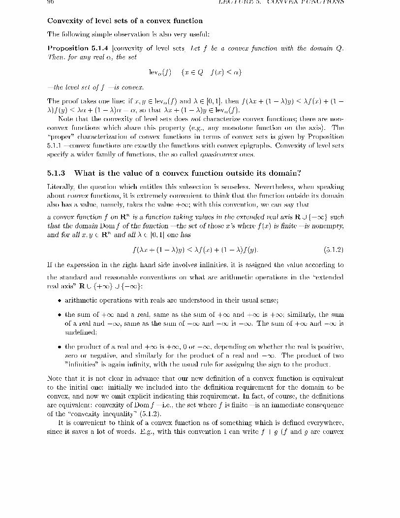
96 LECTURE 5. CONVEX FUNCTIONS
Convexity of level sets of a convex function
The following simple observation is also very useful:
Proposition 5.1.4 [convexity of level sets] Let f be a convex function with the domain Q.Then, for any real �, the set
lev�(f) = fx 2 Q j f(x) � �g{ the level set of f { is convex.
The proof takes one line: if x; y 2 lev�(f) and � 2 [0; 1], then f(�x+ (1� �)y) � �f(x) + (1��)f(y) � ��+ (1� �)� = �, so that �x+ (1� �)y 2 lev�(f).
Note that the convexity of level sets does not characterize convex functions; there are non-convex functions which share this property (e.g., any monotone function on the axis). The\proper" characterization of convex functions in terms of convex sets is given by Proposition5.1.1 { convex functions are exactly the functions with convex epigraphs. Convexity of level setsspecify a wider family of functions, the so called quasiconvex ones.
5.1.3 What is the value of a convex function outside its domain?
Literally, the question which entitles this subsection is senseless. Nevertheless, when speakingabout convex functions, it is extremely convenient to think that the function outside its domainalso has a value, namely, takes the value +1; with this convention, we can say that
a convex function f on Rn is a function taking values in the extended real axis R[ f+1g suchthat the domain Dom f of the function { the set of those x's where f(x) is �nite { is nonempty,and for all x; y 2 Rn and all � 2 [0; 1] one has
f(�x+ (1� �)y) � �f(x) + (1� �)f(y): (5.1.2)
If the expression in the right hand side involves in�nities, it is assigned the value according to
the standard and reasonable conventions on what are arithmetic operations in the \extendedreal axis" R [ f+1g [ f�1g:
� arithmetic operations with reals are understood in their usual sense;
� the sum of +1 and a real, same as the sum of +1 and +1 is +1; similarly, the sumof a real and �1, same as the sum of �1 and �1 is �1. The sum of +1 and �1 isunde�ned;
� the product of a real and +1 is +1, 0 or �1, depending on whether the real is positive,zero or negative, and similarly for the product of a real and �1. The product of two"in�nities" is again in�nity, with the usual rule for assigning the sign to the product.
Note that it is not clear in advance that our new de�nition of a convex function is equivalentto the initial one: initially we included into the de�nition requirement for the domain to beconvex, and now we omit explicit indicating this requirement. In fact, of course, the de�nitionsare equivalent: convexity of Dom f { i.e., the set where f is �nite { is an immediate consequenceof the \convexity inequality" (5.1.2).
It is convenient to think of a convex function as of something which is de�ned everywhere,since it saves a lot of words. E.g., with this convention I can write f + g (f and g are convex
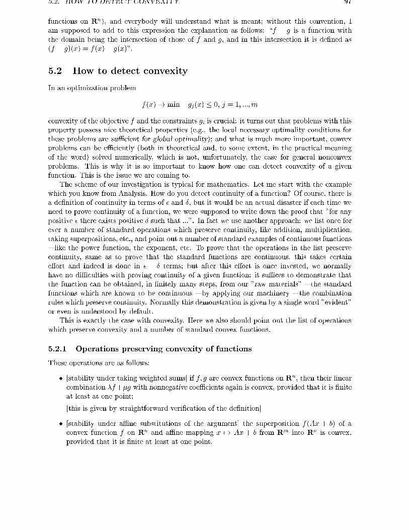
5.2. HOW TO DETECT CONVEXITY 97
functions on Rn), and everybody will understand what is meant; without this convention, Iam supposed to add to this expression the explanation as follows: \f + g is a function withthe domain being the intersection of those of f and g, and in this intersection it is de�ned as(f + g)(x) = f(x) + g(x)".
5.2 How to detect convexity
In an optimization problem
f(x)! min j gj(x) � 0; j = 1; :::;m
convexity of the objective f and the constraints gi is crucial: it turns out that problems with thisproperty possess nice theoretical properties (e.g., the local necessary optimality conditions forthese problems are suÆcient for global optimality); and what is much more important, convexproblems can be eÆciently (both in theoretical and, to some extent, in the practical meaningof the word) solved numerically, which is not, unfortunately, the case for general nonconvexproblems. This is why it is so important to know how one can detect convexity of a givenfunction. This is the issue we are coming to.
The scheme of our investigation is typical for mathematics. Let me start with the examplewhich you know from Analysis. How do you detect continuity of a function? Of course, there isa de�nition of continuity in terms of � and Æ, but it would be an actual disaster if each time weneed to prove continuity of a function, we were supposed to write down the proof that "for anypositive � there exists positive Æ such that ...". In fact we use another approach: we list once forever a number of standard operations which preserve continuity, like addition, multiplication,taking superpositions, etc., and point out a number of standard examples of continuous functions{ like the power function, the exponent, etc. To prove that the operations in the list preservecontinuity, same as to prove that the standard functions are continuous, this takes certaine�ort and indeed is done in � � Æ terms; but after this e�ort is once invested, we normallyhave no diÆculties with proving continuity of a given function: it suÆces to demonstrate thatthe function can be obtained, in �nitely many steps, from our "raw materials" { the standardfunctions which are known to be continuous { by applying our machinery { the combinationrules which preserve continuity. Normally this demonstration is given by a single word "evident"or even is understood by default.
This is exactly the case with convexity. Here we also should point out the list of operationswhich preserve convexity and a number of standard convex functions.
5.2.1 Operations preserving convexity of functions
These operations are as follows:
� [stability under taking weighted sums] if f; g are convex functions on Rn, then their linearcombination �f+�g with nonnegative coeÆcients again is convex, provided that it is �niteat least at one point;
[this is given by straightforward veri�cation of the de�nition]
� [stability under aÆne substitutions of the argument] the superposition f(Ax + b) of aconvex function f on Rn and aÆne mapping x 7! Ax + b from Rm into Rn is convex,provided that it is �nite at least at one point.

98 LECTURE 5. CONVEX FUNCTIONS
[you can prove it directly by verifying the de�nition or by noting that the epigraph ofthe superposition, if nonempty, is the inverse image of the epigraph of f under an aÆnemapping]
� [stability under taking pointwise sup] upper bound sup� f�(�) of any family of convexfunctions on Rn is convex, provided that this bound is �nite at least at one point.
[to understand it, note that the epigraph of the upper bound clearly is the intersectionof epigraphs of the functions from the family; recall that the intersection of any family ofconvex sets is convex]
� [\Convex Monotone superposition"] Let f(x) = (f1(x); :::; fk(x)) be vector-function onRn with convex components fi, and assume that F is a convex function on Rk which ismonotone, i.e., such that z � z0 always implies that F (z) � F (z0). Then the superposition
�(x) = F (f(x)) = F (f1(x); :::; fk(x))
is convex on Rn, provided that it is �nite at least at one point.
Remark 5.2.1 The expression F (f1(x); :::; fk(x)) makes no evident sense at a point xwhere some of fi's are +1. By de�nition, we assign the superposition at such a point thevalue +1.
[To justify the rule, note that if � 2 (0; 1) and x; x0 2 Dom�, then z = f(x); z0 = f(x0) arevectors from Rk which belong to DomF , and due to the convexity of the components off we have
f(�x+ (1� �)x0) � �z + (1� �)z0;
in particular, the left hand side is a vector from Rk { it has no \in�nite entries", and wemay further use the monotonicity of F :
�(�x+ (1� �)x0) = F (f(�x+ (1� �)x0)) � F (�z + (1� �)z0)
and now use the convexity of F :
F (�z + (1� �)z0) � �F (z) + (1� �)F (z0)
to get the required relation
�(�x+ (1� �)x0) � ��(x) + (1� �)�(x0):
]
Imagine how many extra words would be necessary here if there were no convention on the valueof a convex function outside its domain!
Two more rules are as follows:
� [stability under partial minimization] if f(x; y) : Rnx �Rm
y is convex (as a function ofz = (x; y); this is called joint convexity) and the function
g(x) = infyf(x; y)
is proper, i.e., is > �1 everywhere and is �nite at least at one point, then g is convex

5.2. HOW TO DETECT CONVEXITY 99
[this can be proved as follows. We should prove that if x; x0 2 Dom g and x00 =�x + (1 � �)x0 with � 2 [0; 1], then x00 2 Dom g and g(x00) � �g(x) + (1 � �)g(x0).Given positive �, we can �nd y and y0 such that (x; y) 2 Dom f , (x0; y0) 2 Dom f andg(x) + � � f(x; y), g(y0)+ � � f(x0; y0). Taking weighted sum of these two inequalities,we get
�g(x) + (1� �)g(y) + � � �f(x; y) + (1� �)f(x0; y0) �[since f is convex]
� f(�x+ (1� �)x0; �y + (1� �)y0) = f(x00; �y + (1� �)y0)
(the last � follows from the convexity of f). The concluding quantity in the chain is� g(x00), and we get g(x00) � �g(x)+(1��)g(x0)+ �. In particular, x00 2 Dom g (recallthat g is assumed to take only the values from R and the value +1). Moreover, sincethe resulting inequality is valid for all � > 0, we come to g(x00) � �g(x) + (1� �)g(x0),as required.]
� the \conic transformation" of a convex function f on Rn { the function g(y; x) =yf(x=y) { is convex in the half-space y > 0 in Rn+1.
Now we know what are the basic operations preserving convexity. Let us look what are thestandard functions these operations can be applied to. A number of examples was already given,but we still do not know why the functions in the examples are convex. The usual way to checkconvexity of a \simple" { given by a simple formula { function is based on di�erential criteriaof convexity. Let us look what are these criteria.
5.2.2 Di�erential criteria of convexity
From the de�nition of convexity of a function if immediately follows that convexity is one-dimensional property: a proper (i.e., �nite at least at one point) function f on Rn taking valuesin R [ f+1g is convex if and only if its restriction on any line, i.e., any function of the typeg(t) = f(x+ th) on the axis, is either convex, or is identically +1.
It follows that to detect convexity of a function, it, in principle, suÆces to know how to detectconvexity of functions of one variable. This latter question can be resolved by the standardCalculus tools. Namely, in the Calculus they prove the following simple
Proposition 5.2.1 [Necessary and SuÆcient Convexity Condition for smooth functions on theaxis] Let (a; b) be an interval in the axis (we do not exclude the case of a = �1 and/or b = +1).Then
(i) A di�erentiable everywhere on (a; b) function f is convex on (a; b) if and only if itsderivative f 0 is monotonically nondecreasing on (a; b);
(ii) A twice di�erentiable everywhere on (a; b) function f is convex on (a; b) if and only ifits second derivative f 00 is nonnegative everywhere on (a; b).
With the Proposition, you can immediately verify that the functions listed as examples of convexfunctions in Section 5.1.1 indeed are convex. The only diÆculty which you may meet is thatsome of these functions (e.g., xp, p � 1, and �xp, 0 � p � 1, were claimed to be convex on thehalf-interval [0;+1), while the Proposition speaks about convexity of functions on intervals. Toovercome this diÆculty, you may use the following simple
Proposition 5.2.2 Let M be a convex set and f be a function with Dom f =M . Assume thatf is convex on riM and is continuous on M , i.e.,
f(xi)! f(x); i!1;

100 LECTURE 5. CONVEX FUNCTIONS
whenever xi; x 2M and xi ! x as i!1. Then f is convex on M .
Proof of Proposition 5.2.1:
(i), necessity. Assume that f is di�erentiable and convex on (a; b); we should prove thatthen f 0 is monotonically nondecreasing. Let x < y be two points of (a; b), and let us provethat f 0(x) � f 0(y). Indeed, let z 2 (x; y). We clearly have the following representation of zas a convex combination of x and y:
z =y � z
y � xx+
x� z
y � xy;
whence, from convexity,
f(z) � y � z
y � xf(x) +
x� z
y � xf(y);
whencef(z)� f(x)
x� z� f(y)� f(z)
y � z:
Passing here to limit as z ! x+ 0, we get
f 0(x) � (f(y)� f(x)
y � x;
and passing in the same inequality to limit as z ! y � 0, we get
f 0(y) � (f(y)� f(x)
y � x;
whence f 0(x) � f 0(y), as claimed.(i), suÆciency. We should prove that if f is di�erentiable on (a; b) and f 0 is monotonically
nondecreasing on (a; b), then f is convex on (a; b). It suÆces to verify that if x < y,x; y 2 (a; b), and z = �x+ (1� �)y with 0 < � < 1, then
f(z) � �f(x) + (1� �)f(y);
or, which is the same (write f(z) as �f(z) + (1� �)f(z)), that
f(z)� f(x)
�� f(y)� f(z)
1� �:
noticing that z � x = �(y � x) and y � z = (1 � �)(y � x), we see that the inequality weshould prove is equivalent to
f(z)� f(x)
z � x� f(y)� f(z)
y � z:
But in this equivalent form the inequality is evident: by the Lagrange Mean Value Theorem,its left hand side is f 0(�) with some � 2 (x; z), while the right hand one is f 0(�) with some� 2 (z; y). Since f 0 is nondecreasing and � � z � �, we have f 0(�) � f 0(�), and the left handside in the inequality we should prove indeed is � the right hand one.
(ii) is immediate consequence of (i), since, as we know from the very beginning of Calcu-lus, a di�erentiable function { in the case in question, it is f 0 { is monotonically nondecreasingon an interval if and only if its derivative is nonnegative on this interval.
In fact, for functions of one variable there is a di�erential criterion of convexity whichdoes not preassume any smoothness (we shall not prove this criterion):

5.2. HOW TO DETECT CONVEXITY 101
Proposition 5.2.3 [convexity criterion for univariate functions]Let g : R! R[f+1g be a function. Let the domain � = ft j g(t) <1g of the function
be a convex set which is not a singleton, i.e., let it be an interval (a; b) with possibly addedone or both endpoints (�1 � a < b � 1). g is convex if and only if it satis�es the following3 requirements:
1) g is continuous on (a; b);2) g is di�erentiable everywhere on (a; b), excluding, possibly, a countable set of points,
and the derivative g0(t) is nondecreasing on its domain;3) at each endpoint u of the interval (a; b) which belongs to � g is upper semicontinuous:
g(u) � lim supt2(a;b);t!ug(t):
Proof of Proposition 5.2.2: Let x; y 2 M and z = �x + (1 � �)y, � 2 [0; 1], and let usprove that
f(iz) � �f(x) + (1� �)f(y):
As we know from Theorem 2.1.1.(iii), there exist sequences xi 2 riM and yi 2 riM converg-ing, respectively to x and to y. Then zi = �xi + (1 � �)yi converges to z as i ! 1, andsince f is convex on riM , we have
f(zi) � �f(xi) + (1� �)f(yi);
passing to limit and taking into account that f is continuous on M and xi; yi; zi converge,
as i!1, to x; y; z 2M , respectively, we obtain the required inequality.
From Propositions 5.2.1.(ii) and 5.2.2 we get the following convenient necessary and suÆcientcondition for convexity of a smooth function of n variables:
Corollary 5.2.1 [convexity criterion for smooth functions on Rn]Let f : Rn ! R[f+1g be a function. Assume that the domain Q of f is a convex set with
a nonempty interior and that f is
� continuous on Q
and
� twice di�erentiable on the interior of Q.
Then f is convex if and only if its Hessian is positive semide�nite on the interior of Q:
hT f 00(x)h � 0 8x 2 int Q 8h 2 Rn:
Proof.�The "only if" part is evident: if f is convex and x 2 Q0 = int Q, then the
function of one variableg(t) = f(x+ th)
(h is an arbitrary �xed direction in Rn) is convex in certain neighbourhood of the pointt = 0 on the axis (recall that aÆne substitutions of argument preserve convexity). Since fis twice di�erentiable in a neighbourhood of x, g is twice di�erentiable in a neighbourhoodof t = 0, so that g00(0) = hT f 00(x)h � 0 by Proposition 5.2.1.
Now let us prove the "if" part, so that we are given that hT f 00(x)h � 0 for every x 2 int Qand every h 2 Rn, and we should prove that f is convex.
Let us �rst prove that f is convex on the interior Q0 of the domain Q. As we knowfrom Theorem 2.1.1, Q0 is a convex set. Since, as it was already explained, the convexity

102 LECTURE 5. CONVEX FUNCTIONS
of a function on a convex set is one-dimensional fact, all we should prove is that everyone-dimensional function
g(t) = f(x+ t(y � x)); 0 � t � 1
(x and y are from Q0) is convex on the segment 0 � t � 1. Since f is continuous on Q � Q0,g is continuous on the segment; and since f is twice continuously di�erentiable on Q0, g iscontinuously di�erentiable on (0; 1) with the second derivative
g00(t) = (y � x)T f 00(x+ t(y � x))(y � x) � 0:
Consequently, g is convex on [0; 1] (Propositions 5.2.1.(ii) and 5.2.2. Thus, f is convex on
Q0. It remains to note that f , being convex on Q0 and continuous on Q, is convex on Q by
Proposition 5.2.2.
Applying the combination rules preserving convexity to simple functions which pass the \in-�nitesimal' convexity tests, we can prove convexity of many complicated functions. Consider,e.g., an exponential posynomial { a function
f(x) =NXi=1
ci expfaTi xg
with positive coeÆcients ci (this is why the function is called posynomial). How could we provethat the function is convex? This is immediate:
expftg is convex (since its second order derivative is positive and therefore the �rst derivativeis monotone, as required by the in�nitesimal convexity test for smooth functions of one variable);
consequently, all functions expfaTi xg are convex (stability of convexity under aÆne substi-tutions of argument);
consequently, f is convex (stability of convexity under taking linear combinations with non-negative coeÆcients).
And if we were supposed to prove that the maximum of three posynomials is convex? Ok,we could add to our three steps the fourth, which refers to stability of convexity under takingpointwise supremum.
5.3 Gradient inequality
An extremely important property of a convex function is given by the following
Proposition 5.3.1 [Gradient inequality] Let f be a function taking �nite values and the value+1, x be an interior point of the domain of f and Q be a convex set containing x. Assume that
� f is convex on Q
and
� f is di�erentiable at x,
and let rf(x) be the gradient of the function at x. Then the following inequality holds:
(8y 2 Q) : f(y) � f(x) + (y � x)Trf(x): (5.3.1)

5.3. GRADIENT INEQUALITY 103
Geometrically: the graph
f(y; t) 2 Rn+1 j y 2 Dom f \Q; t = f(y)gof the function f restricted at the set Q is above the graph
f(y; t) 2 Rn+1 j t = f(x) + (y � x)Trf(x)gof the linear form tangent to f at x.
Proof. Let y 2 Q. There is nothing to prove if y 62 Dom f (since there the right hand side inthe gradient inequality is +1), same as there is nothing to prove when y = x. Thus, we canassume that y 6= x and y 2 Dom f . Let us set
y� = x+ �(y � x); 0 < � � 1;
so that y1 = y and y� is an interior point of the segment [x; y] for 0 < � < 1. Now let us use thefollowing extremely simple
Lemma 5.3.1 Let x; x0; x00 be three distinct points with x0 2 [x; x00], and let f beconvex and �nite on [x; x00]. Then
f(x0)� f(x)
k x0 � x k � f(x00)� f(x)
k x00 � x k : (5.3.2)
Proof of the Lemma. We clearly have
x0 = x+ �(x00 � x); � =k x0 � x kk x00 � x k 2 (0; 1)
or, which is the same,x0 = (1� �)x+ �x00:
From the convexity inequality
f(x0) � (1� �)f(x) + �f(x00);
or, which is the same,
f(x0)� f(x) � �(f(x00)� f(x0)):
Dividing by � and substituting the value of �, we come to (5.3.2).
Applying the Lemma to the triple x; x0 = y� ; x00 = y, we get
f(x+ �(y � x))� f(x)
� k y � x k � f(y)� f(x)
k y � x k ;
as � ! +0, the left hand side in this inequality, by the de�nition of the gradient, tends tok y � x k�1 (y � x)Trf(x), and we get
k y � x k�1 (y � x)Trf(x) �k y � x k�1 (f(y)� f(x));
or, which is the same,(y � x)Trf(x) � f(y)� f(x);
this is exactly the inequality (5.3.1).

104 LECTURE 5. CONVEX FUNCTIONS
To conclude the story about the Gradient inequality, it is worthy of mentioning thatin the case when Q is convex set with a nonempty interior and f is continuous on Q anddi�erentiable on int Q, f is convex on Q if and only if the Gradient inequality (5.3.1) is validfor every pair x 2 int Q and y 2 Q.
Indeed, the "only if" part, i.e., the implication
convexity of f ) Gradient inequality for all x 2 int Q and all y 2 Qis given by Proposition 5.3.1. To prove the "if" part, i.e., to establish the implication inverseto the above, assume that f satis�es the Gradient inequality for all x 2 int Q and all y 2 Q,and let us verify that f is convex on Q. It suÆces to prove that f is convex on the interiorQ0 of the set Q (see Proposition 5.2.2; recall that by assumption f is continuous on Q andQ is convex). To prove that f is convex on Q0, note that Q0 is convex (Theorem 2.1.1) andthat, due to the Gradient inequality, on Q0 f is the upper bound of the family of aÆne (andtherefore convex) functions:
f(y) = supx2Q0
fx(y); fx(y) = f(x) + (y � x)Trf(x):
5.4 Boundedness and Lipschitz continuity of a convex
function
Convex functions possess nice local properties.
Theorem 5.4.1 [local boundedness and Lipschitz continuity of convex function]Let f be a convex function and let K be a closed and bounded set contained in the
relative interior of the domain Dom f of f . Then f is Lipschitz continuous on K { thereexists constant L { the Lipschitz constant of f on K { such that
jf(x)� f(y)j � Ljx� yj 8x; y 2 K: (5.4.1)
In particular, f is bounded on K.
Remark 5.4.1 All three assumptions on K { (1) closedness, (2) boundedness and the as-sumption (3) K � ri Dom f { are essential, as it is seen from the following three examples:
� f(x) = 1=x; DomF = (0;+1),K = (0; 1]. We have (2), (3) and not (1); f is neitherbounded, nor Lipschitz continuous on K.
� f(x) = x2, Dom f = R, K = R. We have (1), (3) and not (2); f is neither boundednor Lipschitz continuous on K.
� f(x) = �px, Dom f = [0;+1), K = [0; 1]. We have (1), (2) and not (3); f is notLipschitz continuous on K 1), although is bounded. With properly chosen convexfunction f of two variables and non-polyhedral compact domain (e.g., with Dom fbeing the unit circle), we could demonstrate also that lack of (3), even in presence of(1) and (2), may cause unboundedness of f at K as well.
Remark 5.4.2 Theorem 5.4.1 says that a convex function f is bounded on every compact(i.e., closed and bounded) subset of the relative interior of Dom f . In fact there is muchstronger statement on the below boundedness of f : f is below bounded on any boundedsubset of Rn!.
Proof of Theorem 5.4.1. We shall start with the following local version of the Theorem.
1)indeed, we have limt!+0f(0)�f(t)
t = limt!+0 t�1=2 = +1, while for a Lipschitz continuous f the ratios
t�1(f(0) � f(t)) should be bounded

5.4. BOUNDEDNESS AND LIPSCHITZ CONTINUITY OF A CONVEX FUNCTION 105
Proposition 5.4.1 Let f be a convex function, and let �x be a point from the relative interiorof the domain Dom f of f . Then
(i) f is bounded at �x: there exists a positive r such that f is bounded in the r-neighbourhood Ur(�x) of �x in the aÆne span of Dom f :
9r > 0; C : jf(x)j � C 8x 2 Ur(�x) = fx 2 A�(Dom f) j k x� �x k� rg;
(ii) f is Lipschitz continuous at �x, i.e., there exists a positive � and a constant L suchthat
jf(x)� f(x0)j � L k x� x0 k 8x; x0 2 U�(�x):
Implication \Proposition 5.4.1 ) Theorem 5.4.1" is given by standard Analysis rea-soning. All we need is to prove that if K is a bounded and closed (i.e., a compact) subsetof ri Dom f , then f is Lipschitz continuous on K (the boundedness of f on K is an evidentconsequence of its Lipschitz continuity on K and boundedness of K). Assume, on contrary,that f is not Lipschitz continuous on K; then for every integer i there exists a pair of pointsxi; yi 2 K such that
f(xi)� f(yi) � ijxi � yij: (5.4.2)
Since K is compact, passing to a subsequence we can ensure that xi ! x 2 K and yi !y 2 K. By Proposition 5.4.1 the case x = y is impossible { by Proposition f is Lipschitzcontinuous in a neighbourhood B of x = y; since xi ! x; yi ! y, this neighbourhood shouldcontain all xi and yi with large enough indices i; but then, from the Lipschitz continuityof f in B, the ratios (f(xi) � f(yi))=jxi � yij form a bounded sequence, which we know isnot the case. Thus, the case x = y is impossible. The case x 6= y is \even less possible"{ since, by Proposition, f is continuous on Dom f at both the points x and y (note thatLipschitz continuity at a point clearly implies the usual continuity at it), so that we wouldhave f(xi) ! f(x) and f(yi) ! f(y) as i ! 1. Thus, the left hand side in (5.4.2) remainsbounded as i ! 1. In the right hand side one factor { i { tends to 1, and the other onehas a nonzero limit jx � yj, so that the right hand side tends to 1 as i ! 1; this is thedesired contradiction.Proof of Proposition 5.4.1.
10. We start with proving the above boundedness of f in a neighbourhood of �x. This isimmediate: we know that there exists a neighbourhood U�r(�x) which is contained in Dom f(since, by assumption, �x is a relative interior point of Dom f). Now, we can �nd a smallsimplex � of the dimension m = dim A�(Dom f) with the vertices x0; :::; xm in U�r(�x) insuch a way that �x will be a convex combination of the vectors xi with positive coeÆcients,even with the coeÆcients 1=(m+ 1):
�x =mXi=0
1
m+ 1xi 2):
2to see that the required � exists, let us act as follows: �rst, the case of Dom f being a singleton is evident, sothat we can assume that Dom f is a convex set of dimension m � 1. Let us take arbitrary aÆne basis y0; :::; ym inM = A�(Dom f) and then pass from this basis to the set z0 = y0; z1 = y0+�(y1�y0); z2 = y0+�(y2�y0); :::; zm =y0 + �(ym � y0) with some � > 0. The vectors zi clearly belong to M and form an aÆne basis (the latter followsfrom the fact that the vectors zi � z0, i = 1; :::; m, are � times the vectors yi � y0; the latter vectors form a basisin the linear subspace L such that M = y0+L, Theorem 1.3.1; consequently, the vectors zi� z0, i = 1; :::; m, alsoform a basis in L, whence, by the same Corollary, z0; :::; zm form am aÆne basis in M). Choosing � > 0 smallenough, we may enforce all the vectors z0; :::; zm be in the (�r=10)-neighbourhood of the vector z0. Now let �0 bethe convex hull of z0; :::; zm; this is a simplex with the vertices contained in the neighbourhood of z0 of the radius�r=10 (of course, we are speaking about the ball in M). This neighbourhood is an intersection of a Euclidean ball,which is a convex set, and M , which also is convex; therefore the neighbourhood is convex. Since the verticesof �0 are contained in it, the entire �0 is contained in the neighbourhood. Now let �z = (m + 1)�1
Pmi=0 zi; �
0
clearly is contained in the 2 � (�r=10) = �r=5 neighbourhood of �z in M . Setting � = [�x � �z] + �0, we get the

106 LECTURE 5. CONVEX FUNCTIONS
We know that �x is the point from the relative interior of � (see the proof of Theorem2.1.1.(ii)); since � spans the same aÆne set as Dom f (m is the dimension of A�(Dom f)!),it means that � contains Ur(�x) with certain r > 0. Now, in
� = fmXi=0
�ixi j �i � 0;Xi
�i = 1g
f is bounded from above by the quantity max0�i�m f(xi) by Jensen's inequality:
f(mXi=0
�ixi) �mXi=0
�if(xi) � maxif(xi):
Consequently, f is bounded from above, by the same quantity, in Ur(�x).20. Now let us prove that if f is above bounded, by some C, in Ur(�x), then it in fact
is below bounded in this neighbourhood (and, consequently, is bounded in Ur). Indeed, letx 2 Ur, so that x 2 A�(Dom f) and k x� �x k� r. Setting x0 = �x� [x� �x] = 2�x� x, we getx0 2 A�(Dom f) and k x0 � �x k=k x� �x k� r, so that x0 2 Ur. Since �x = 1
2 [x+ x0], we have
2f(�x) � f(x) + f(x0);
whencef(x) � 2f(�x)� f(x0) � 2f(�x)� C; x 2 Ur(�x);
and f indeed is below bounded in Ur.(i) is proved.30. (ii) is an immediate consequence of (i) and Lemma 5.3.1. Indeed, let us prove that f
is Lipschitz continuous in the neighbourhood Ur=2(�x), where r > 0 is such that f is boundedin Ur(�x) (we already know from (i) that the required r does exist). Let jf j � C in Ur, and letx; x0 2 Ur=2, x 6= x0. Let us extend the segment [x; x0] through the point x0 until it reaches,at certain point x00, the (relative) boundary of Ur; then we will get
x0 2 (x; x00); k x00 � �x k= r:
From (5.3.2) we have
f(x0)� f(x) �k x0 � x k f(x00)� f(x)
k x00 � x k :
The second factor in the right hand side does not exceed the quantity (2C)=(r=2) = 4C=r;indeed, the numerator is, in absolute value, at most 2C (since jf j is bounded by C in Ur andboth x; x00 belong to Ur), and the denominator is at least r=2 (indeed, x is at the distanceat most r=2 from �x, and x00 is at the distance exactly r from �x, so that the distance betweenx and x00, by the triangle inequality, is at least r=2). Thus, we have
f(x0)� f(x) � (4C=r) k x0 � x k; x; x0 2 Ur=2;swapping x and x0, we come to
f(x)� f(x0) � (4C=r) k x0 � x k;simplex with the vertices xi = zi+ �x� �z which is contained in the �r=5-neighbourhood of �x in M and is such that(m+ 1)�1
Pmi=0 xi � (m+ 1)�1
Pmi=0[zi + �x� �z] = �z + �x� �z = �x, as required.
I gave this awful \explanation" to demonstrate how many words we need to make rigorous \evident" recommen-dations like \let us take a small simplex with the average of vertices equal to �x". The \explanations" of this typeshould (and will) be omitted, since they kill even the most clear reasoning. Note, anyhow, that in mathematicswe in fact should be able to explain, on a request, what does it mean \to take a small simplex" and how one can\take" it. Needless to say, you are supposed to be able to do this routine work by yourselves; and to this end youshould remember what is the exact meaning of the words we are using and what are the basic relations betweenthe corresponding concepts.
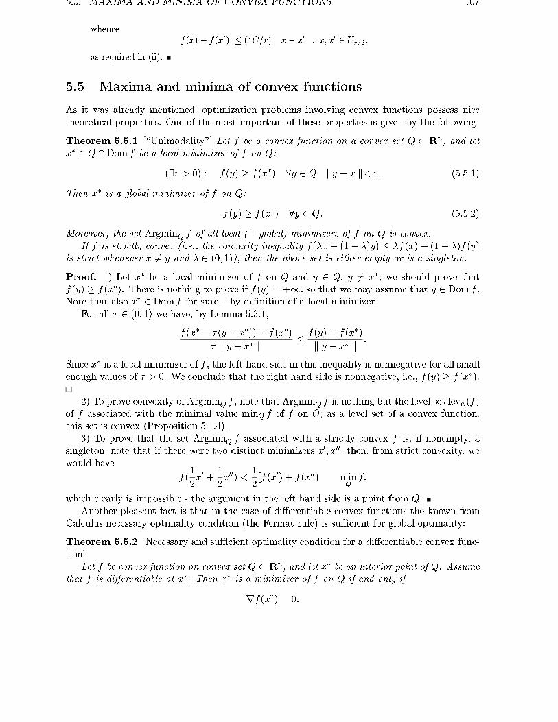
5.5. MAXIMA AND MINIMA OF CONVEX FUNCTIONS 107
whencejf(x)� f(x0)j � (4C=r) k x� x0 k; x; x0 2 Ur=2;
as required in (ii).
5.5 Maxima and minima of convex functions
As it was already mentioned, optimization problems involving convex functions possess nicetheoretical properties. One of the most important of these properties is given by the following
Theorem 5.5.1 [\Unimodality"] Let f be a convex function on a convex set Q � Rn, and letx� 2 Q \Dom f be a local minimizer of f on Q:
(9r > 0) : f(y) � f(x�) 8y 2 Q; k y � x k< r: (5.5.1)
Then x� is a global minimizer of f on Q:
f(y) � f(x�) 8y 2 Q: (5.5.2)
Moreover, the set ArgminQ f of all local (� global) minimizers of f on Q is convex.If f is strictly convex (i.e., the convexity inequality f(�x+ (1� �)y) � �f(x) + (1� �)f(y)
is strict whenever x 6= y and � 2 (0; 1)), then the above set is either empty or is a singleton.
Proof. 1) Let x� be a local minimizer of f on Q and y 2 Q, y 6= x�; we should prove thatf(y) � f(x�). There is nothing to prove if f(y) = +1, so that we may assume that y 2 Dom f .Note that also x� 2 Dom f for sure { by de�nition of a local minimizer.
For all � 2 (0; 1) we have, by Lemma 5.3.1,
f(x� + �(y � x�))� f(x�)
� k y � x� k � f(y)� f(x�)
k y � x� k :
Since x� is a local minimizer of f , the left hand side in this inequality is nonnegative for all smallenough values of � > 0. We conclude that the right hand side is nonnegative, i.e., f(y) � f(x�).
2) To prove convexity of ArgminQ f , note that ArgminQ f is nothing but the level set lev�(f)of f associated with the minimal value minQ f of f on Q; as a level set of a convex function,this set is convex (Proposition 5.1.4).
3) To prove that the set ArgminQ f associated with a strictly convex f is, if nonempty, asingleton, note that if there were two distinct minimizers x0; x00, then, from strict convexity, wewould have
f(1
2x0 +
1
2x00) <
1
2[f(x0) + f(x00) == min
Qf;
which clearly is impossible - the argument in the left hand side is a point from Q!Another pleasant fact is that in the case of di�erentiable convex functions the known from
Calculus necessary optimality condition (the Fermat rule) is suÆcient for global optimality:
Theorem 5.5.2 [Necessary and suÆcient optimality condition for a di�erentiable convex func-tion]
Let f be convex function on convex set Q � Rn, and let x� be an interior point of Q. Assumethat f is di�erentiable at x�. Then x� is a minimizer of f on Q if and only if
rf(x�) = 0:

108 LECTURE 5. CONVEX FUNCTIONS
Proof. As a necessary condition for local optimality, the relation rf(x�) = 0 is known fromCalculus; it has nothing in common with convexity. The essence of the matter is, of course, thesuÆciency of the condition rf(x�) = 0 for global optimality of x� in the case of convex f . ThissuÆciency is readily given by the Gradient inequality (5.3.1): by virtue of this inequality anddue to rf(x�) = 0,
f(y) � f(x�) + (y � x�)rf(x�) = f(x�)
for all y 2 Q.Remark 5.5.1 A natural question is what happens if x� in the above statement is not neces-sarily an interior point of Q. Thus, assume that x� is an arbitrary point of a convex set Q andthat f is convex on Q and di�erentiable at x� (the latter means exactly that Dom f contains aneighbourhood of x� and f possesses the �rst order derivative at x�). Under these assumptions,when x� is a minimizer of f on Q?
The answer is as follows: let
TQ(x�) = fh 2 Rn j x� + th 2 Q 8 small enough t > 0g
be the tangent cone of Q at x�; geometrically, this is the set of all directions leading from x�
inside Q, so that a small enough positive step from x� along the direction keeps the point in Q.From the convexity of Q it immediately follows that the tangent cone indeed is a convex cone(not necessary closed). E.g., when x� is an interior point of Q, then the tangent cone to Q atx� clearly is the entire Rn. A more interesting example is the tangent cone to a polyhedral set
Q = fx j aTi x � bi; i = 1; :::;mg; (5.5.3)
for x� 2 Q the corresponding tangent cone clearly is the polyhedral cone
fh j aTi h � 0 8i : aTi x� = big (5.5.4)
corresponding to the active at x� (i.e., satis�ed at the point as equalities rather than as strictinequalities) constraints aTi x � bi from the description of Q.
Now, for the functions in question (i.e., convex on Q and di�erentiable at x�) the necessaryand suÆcient condition for x� to be a minimizer of f on Q is as follows:
(*) the derivative of f taken at x� along every direction from TQ(x�) should be nonnegative:
hTrf(x�) � 0 8h 2 TQ(x�):
The proof is immediate. The necessity is an evident fact which has nothing in commonwith convexity: assuming that x� is a local minimizer of f on Q, we note that if there wereh 2 TQ(x�) with hTrf(x�) < 0, then we would have
f(x� + th) < f(x�)
for all small enough positive t. On the other hand, x�+th 2 Q for all small enough positive tdue to h 2 TQ(x�). Combining these observations, we conclude that in every neighbourhoodof x� there are points from Q with strictly better than the one at x� values of f ; thiscontradicts the assumption that x� is a local minimizer of f on Q.
The suÆciency is given by the Gradient Inequality, exactly as in the case when x� is an
interior point of Q.

5.5. MAXIMA AND MINIMA OF CONVEX FUNCTIONS 109
Condition (*) says that whenever f is convex on Q and di�erentiable at x� 2 Q, the necessaryand suÆcient condition for x� to be a minimizer of f on Q is that the linear form given bythe gradient rf(x�) of f at x� should be nonnegative at all directions from the tangent coneTQ(x�). The linear forms nonnegative at all directions from the tangent cone also form a cone;it is called the cone normal to Q at x� and is denoted NQ(x�). Thus, (*) says that the necessaryand suÆcient condition for x� to minimize f on Q is the inclusion rf(x�) 2 NQ(x�). Whatdoes this condition actually mean, it depends on what is the normal cone: whenever we have anexplicit description of it, we have an explicit form of the optimality condition.
E.g., when TQ(x�) = Rn (it is the same as to say that x� is an interior point of Q), then thenormal cone is comprised of the linear forms nonnegative at the entire space, i.e., it is the trivialcone f0g; consequently, for the case in question the optimality condition becomes the Fermatrule rf(x�) = 0, as we already know.
When Q is the polyhedral set (5.5.3), the normal cone is the polyhedral cone (5.5.4); it iscomprised of all directions which have nonpositive inner products with all ai coming from theactive, in the aforementioned sense, constraints. The normal cone is comprised of all vectorswhich have nonnegative inner products with all these directions, i.e., of vectors a such that theinequality hTa � 0 is a consequence of the inequalities hT ai � 0, i 2 I(x�) � fi j aTi x� = big.From the Homogeneous Farkas Lemma we conclude that the normal cone is simply the conichull of the vectors �ai, i 2 I(x�). Thus, in the case in question (*) reads:
x� 2 Q is a minimizer of f on Q if and only if there exist nonnegative reals ��i associatedwith \active" (those from I(x�)) values of i such that
rf(x�) + Xi2I(x�)
��i ai = 0:
These are the famous Karush-Kuhn-Tucker optimality conditions; in the mean time we shallprove that these conditions are necessary for optimality in an essentially wider situation.
The indicated results demonstrate that the fact that a point x� 2 Dom f is a global minimizerof a convex function f depends only on the local behaviour of f at x�. This is not the case withmaximizers of a convex function. First of all, such a maximizer, if exists, in all nontrivial casesshould belong to the boundary of the domain of the function:
Theorem 5.5.3 Let f be convex, and let Q be the domain of f . Assume that f attains itsmaximum on Q at a point x� from the relative interior of Q. Then f is constant on Q.
Proof. Let y 2 Q; we should prove that f(y) = f(x�). There is nothing to prove if y = x�, sothat we may assume that y 6= x�. Since, by assumption, x� 2 riQ, we can extend the segment[x�; y] through the endpoint x�, keeping the left endpoint of the segment in Q; in other words,there exists a point y0 2 Q such that x� is an interior point of the segment [y0; y]:
x� = �y0 + (1� �)y
for certain � 2 (0; 1). From the de�nition of convexity
f(x�) � �f(y0) + (1� �)f(y):
Since both f(y0) and f(y) do not exceed f(x�) (x� is a maximizer of f on Q!) and boththe weights � and 1 � � are strictly positive, the indicated inequality can be valid only iff(y0) = f(y) = f(x�).
The next theorem gives further information on maxima of convex functions:

110 LECTURE 5. CONVEX FUNCTIONS
Theorem 5.5.4 Let f be a convex function on Rn and E be a subset of Rn. Then
supConvE
f = supEf: (5.5.5)
In particular, if S � Rn is convex and compact set, then the upper bound of f on S is equal tothe upper bound of f on the set of extreme points of S:
supSf = sup
Ext(S)f (5.5.6)
Proof. To prove (5.5.5), let x 2 ConvE, so that x is a convex combination of points from E(Theorem 2.1.3 on the structure of convex hull):
x =Xi
�ixi [xi 2 E; �i � 0;Xi
�i = 1]:
Applying Jensen's inequality (Proposition 5.1.3), we get
f(x) �Xi
�if(xi) �Xi
�i supEf = sup
Ef;
so that the left hand side in (5.5.5) is � the right hand one; the inverse inequality is evident,since ConvE � E.
To derive (5.5.6) from (5.5.5), it suÆces to note that from the Krein-Milman Theorem(Theorem 4.2.1) for a convex compact set S one has S = ConvExt(S).
The last theorem on maxima of convex functions is as follows:
Theorem 5.5.5�
Let f be a convex function such that the domain Q of f is closed anddoes not contain lines. Then
(i) If the setArgmax
Qf � fx 2 Q j f(x) � f(y)8y 2 Qg
of global maximizers of f is nonempty, then it intersects the set Ext(Q) of the extreme pointsof Q, so that at least one of the maximizers of f is an extreme point of Q;
(ii) If the set Q is polyhedral and f is above bounded on Q, then the maximum of f onQ is achieved: ArgmaxQ f 6= ;.Proof. Let us start with (i). We shall prove this statement by induction on the dimensionof Q. The base dim Q = 0, i.e., the case of a singleton Q, is trivial, since here Q = ExtQ =ArgmaxQ f . Now assume that the statement is valid for the case of dim Q � p, and let usprove that it is valid also for the case of dim Q = p + 1. Let us �rst verify that the setArgmaxQ f intersects with the (relative) boundary of Q. Indeed, let x 2 ArgmaxQ f . Thereis nothing to prove if x itself is a relative boundary point of Q; and if x is not a boundarypoint, then, by Theorem 5.5.3, f is constant on Q, so that ArgmaxQ f = Q; and since Q isclosed, any relative boundary point of Q (such a point does exist, since Q does not containlines and is of positive dimension) is a maximizer of f on Q, so that here again ArgmaxQ fintersects @riQ.
Thus, among the maximizers of f there exists at least one, let it be x, which belongsto the relative boundary of Q. Let H be the hyperplane which properly supports Q at x(see Section 4.1), and let Q0 = Q \ H . The set Q0 is closed and convex (since Q and Hare), nonempty (it contains x) and does not contain lines (since Q does not). We havemaxQ f = f(x) = maxQ0 f (note that Q0 � Q), whence
; 6= ArgmaxQ0
f � ArgmaxQ
f:

5.6. SUBGRADIENTS AND LEGENDRE TRANSFORMATION 111
Same as in the proof of the Krein-Milman Theorem (Theorem 4.2.1), we have dim Q0 <dim Q. In view of this inequality we can apply to f and Q0 our inductive hypothesis to get
Ext(Q0) \ ArgmaxQ0
f 6= ;:
Since Ext(Q0) � Ext(Q) by Lemma 4.2.2 and, as we just have seen, ArgmaxQ0 f �ArgmaxQ f , we conclude that the set Ext(Q) \ ArgmaxQ f is not smaller than Ext(Q0) \ArgmaxQ0 f and is therefore nonempty, as required.
To prove (ii), let us use the known to us from Lecture 4 results on the structure of apolyhedral convex set:
Q = Conv(V ) + Cone (R);
where V and R are �nite sets. We are about to prove that the upper bound of f on Q isexactly the maximum of f on the �nite set V :
8x 2 Q : f(x) � maxv2V
f(v): (5.5.7)
This will mean, in particular, that f attains its maximum on Q { e.g., at the point of Vwhere f attains its maximum on V .
To prove the announced statement, I �rst claim that if f is above bounded on Q, thenevery direction r 2 Cone (R) is descent for f , i.e., is such that any step in this directiontaken from any point x 2 Q decreases f :
f(x+ tr) � f(x) 8x 2 Q8t � 0: (5.5.8)
Indeed, if, on contrary, there were x 2 Q, r 2 R and t � 0 such that f(x + tr) > f(x), wewould have t > 0 and, by Lemma 5.3.1,
f(x+ sr) � f(x) +s
t(f(x+ tr) � f(x)); s � t:
Since x 2 Q and r 2 Cone (R), x+ sr 2 Q for all s � 0, and since f is above bounded on Q,the left hand side in the latter inequality is above bounded, while the right hand one, due tof(x+ tr) > f(x), goes to +1 as s!1, which is the desired contradiction.
Now we are done: to prove (5.5.7), note that a generic point x 2 Q can be representedas
x =Xv2V
�vv + r [r 2 Cone (R);Xv
�v = 1; �v � 0];
and we havef(x) = f(
Pv2V �vv + r)
� f(P
v2V �vv) [by (5.5.8)]� P
v2V �vf(v) [Jensen's Inequality]� maxv2V f(v)
5.6 Subgradients and Legendre transformation
This Section is not obligatory!According to one of two equivalent de�nitions, a convex function f onRn is a function takingvalues in R [ f+1g such that the epigraph
Epi(f) = f(t; x) 2 Rn+1 j t � f(x)gis a nonempty convex set. Thus, there is no essential di�erence between convex functionsand convex sets: convex function generates a convex set { its epigraph { which of courseremembers everything about the function. And the only speci�c property of the epigraph as
112 LECTURE 5. CONVEX FUNCTIONS
a convex set is that it has a recessive direction { namely, e = (1; 0) { such that the intersectionof the epigraph with any line directed by h is either empty, or is a closed ray. Whenever anonempty convex set possesses such a property with respect to certain direction, it can berepresented, in properly chosen coordinates, as the epigraph of some convex function. Thus,a convex function is, basically, nothing but a way to look, in the literal meaning of the latterverb, at a convex set.
Now, we know that \actually good" convex sets are closed ones: they possess a lot ofimportant properties (e.g., admit a good outer description) which are not shared by arbitraryconvex sets. It means that among convex functions there also are \actually good" ones {those with closed epigraphs. Closedness of the epigraph can be \translated" to the functionallanguage and there becomes a special kind of continuity { lower semicontinuity:
De�nition 5.6.1 [Lower semicontinuity] Let f be a function (not necessarily convex) de�nedon Rn and taking values in R [ f+1g. We say that f is lower semicontinuous at a point�x, if for any sequence of points fxig converging to �x one has
f(�x) � lim infi!1
f(xi)
(here, of course, lim inf of a sequence with all terms equal to +1 is +1).f is called lower semicontinuous, if it is lower semicontinuous at every point.
A trivial example of a lower semicontinuous function is a continuous one. Note, however,that a semicontinuous function is not obliged to be continuous; what it is obliged, is to makeonly \jumps down". E.g., the function
f(x) =
�0; x 6= 0a; x = 0
is lower semicontinuous if a � 0 ("jump down at x = 0 or no jump at all"), and is not lowersemicontinuous if a > 0 ("jump up").
The following statement links lower semicontinuity with the geometry of the epigraph:
Proposition 5.6.1 A function f de�ned on Rn and taking values from R[f+1g is lowersemicontinuous if and only if its epigraph is closed (e.g., due to its emptiness).
I shall not prove this statement, same as most of other statements in this Section; I stronglybelieve that those that curious to read this Section de�nitely are capable to restore (verysimple) proofs I am skipping.
An immediate consequence of the latter proposition is as follows:
Corollary 5.6.1 The upper bound
f(x) = sup�2A
f�(x)
of arbitrary family of lower semicontinuous functions is lower semicontinuous.[from now till the end of the Section, if the opposite is not explicitly stated, \a function"means \a function de�ned on the entire Rn and taking values in R [ f+1g"]Indeed, the epigraph of the upper bound is the intersection of the epigraphs of the functionsforming the bound, and the intersection of closed sets always is closed.
Now let us look at convex lower semicontinuous functions; according to our generalconvention, \convex" means \satisfying the convexity inequality and �nite at least in onepoint", or, which is the same, \with convex nonempty epigraph"; and as we just have seen,\lower semicontinuous" means \with closed epigraph". Thus, we are interested in functionswith closed convex nonempty epigraphs; to save words, let us call these functions proper.
What we are about to do is to translate to the functional language several constructionsand results related to convex sets. In the usual life, a translation (e.g. of poetry) typicallyresults in something less rich than the original; in contrast to this, in mathematics this is apowerful source of new ideas and constructions.

5.6. SUBGRADIENTS AND LEGENDRE TRANSFORMATION 113
\Outer description" of a proper function. We know that a closed convex set isintersection of closed half-spaces. What does this fact imply when the set is the epigraphof a proper function f? First of all, note that the epigraph is not a completely arbitraryconvex set: it has a recessive direction e = (1; 0) { the basic orth of the t-axis in the spaceof variables t 2 R; x 2 Rn where the epigraph lives. This direction, of course, should berecessive for any closed half-space
(�) � = f(t; x) j �t � dTx� ag [j�j+ jdj > 0]
containing Epi(f) (note that what is written in the right hand side of the latter relation,is one of many universal forms of writing down a general nonstrict linear inequality in thespace where the epigraph lives; this is the form the most convenient for us now). Thus, eshould be a recessive direction of � � Epi(f); as it is immediately seen, recessivity of e for� means exactly that � � 0. Thus, speaking about closed half-spaces containing Epi(f), wein fact are considering some of the half-spaces (*) with � � 0.
Now, there are two essentially di�erent possibilities for � to be nonnegative { (A) to bepositive, and (B) to be zero. In the case of (B) the boundary hyperplane of � is \vertical"{ it is parallel to e, and in fact it \bounds" only x { � is comprised of all pairs (t; x) with xbelonging to certain half-space in the x-subspace and t being arbitrary real. These \vertical"subspace will be of no interest for us.
The half-spaces which indeed are of interest for us are the \nonvertical" ones: those givenby the case (A), i.e., with � > 0. For a non-vertical half-space �, we always can divide theinequality de�ning � by � and to make � = 1. Thus, a \nonvertical" candidate to the roleof a closed half-space containing Epi(f) always can be written down as
(��) � = f(t; x) j t � dTx� ag;
i.e., can be represented as the epigraph of an aÆne function of x.Now, when such a candidate indeed is a half-space containing Epi(f)? The answer is
clear: it is the case if and only if the aÆne function dTx � a everywhere in Rn is � f(�) {as we shall say, \is an aÆne minorant of f"; indeed, the smaller is the epigraph, the largeris the function. If we knew that Epi(f) { which de�nitely is the intersection of all closedhalf-spaces containing Epi(f) { is in fact the intersection of already nonvertical closed half-spaces containing Epi(f), or, which is the same, the intersection of the epigraphs of all aÆneminorants of f , we would be able to get a nice and nontrivial result:
(!) a proper convex function is the upper bound of aÆne functions { all its aÆneminorants.
(indeed, we already know that it is the same { to say that a function is an upper bound ofcertain family of functions, and to say that the epigraph of the function is the intersectionof the epigraphs of the functions of the family).
(!) indeed is true:
Proposition 5.6.2 A proper convex function f is the upper bound of all its aÆne minorants.Moreover, at every point �x 2 ri Dom f from the relative interior of the domain f f is evennot the upper bound, but simply the maximum of its minorants: there exists an aÆne functionf�x(x) which is � f(x) everywhere in Rn and is equal to f at x = �x.
Proof. I. We start with the \Moreover" part of the statement; this is the key to the entirestatement. Thus, we are about to prove that if �x 2 ri Dom f , then there exists an aÆnefunction f�x(x) which is everywhere � f(x), and at x = �x the inequality becomes an equality.
I.10 First of all, we easily can reduce the situation to the one when Dom f is full-dimensional. Indeed, by shifting f we may make the aÆne span A�(Dom f) of the domainof f to be a linear subspace L in Rn; restricting f onto this linear subspace, we clearly get a

114 LECTURE 5. CONVEX FUNCTIONS
proper function on L. If we believe that our statement is true for the case when the domainof f is full-dimensional, we can conclude that there exists an aÆne function
dTx� a [x 2 L]on L (d 2 L) such that
f(x) � dTx� a 8x 2 L; f(�x) = dT �x� a:
The aÆne function we get clearly can be extended, by the same formula, from L on theentire Rn and is a minorant of f on the entire Rn { outside of L � Dom f f simply is +1!This minorant on Rn is exactly what we need.
I.20. Now let us prove that our statement is valid when Dom f is full-dimensional, sothat �x is an interior point of the domain of f . Let us look at the point y = (f(�x); �x). Thisis a point from the epigraph of f , and I claim that it is a point from the relative boundaryof the epigraph. Indeed, if y were a relative interior point of Epi(f), then, taking y0 = y+ e,we would get a segment [y0; y] containing in Epi(f); since the endpoint y of the segment isassumed to be relative interior for Epi(f), we could extend this segment a little through thisendpoint, not leaving Epi(f); but this clearly is impossible, since the t-coordinate of the newendpoint would be < f(�x), and the x-component of it still would be �x.
Thus, y is a point from the relative boundary of Epi(f). Now I claim that y0 is an interiorpoint of Epi(f). This is immediate: we know from Theorem 5.4.1 that f is continuous at �x,so that there exists a neighbourhood U of �x in A�(Dom f) = Rn such that f(x) � f(�x+0:5)whenever x 2 U , or, in other words, the set
V = f(t; x) j x 2 U; t > f(�x) + 0:5gis contained in Epi(f); but this set clearly contains a neighbourhood of y0 in Rn+1.
Now let us look at the supporting linear form to Epi(f) at the point y of the relativeboundary of Epi(f). This form gives us a linear inequality on Rn+1 which is satis�edeverywhere on Epi(f) and becomes equality at y; besides this, the inequality is not equalityidentically on Epi(f), it is strict somewhere on Epi(f). Without loss of generality we mayassume that the inequality is of the form
(+) �t � dTx� a:
Now, since our inequality is satis�ed at y0 = y + e and becomes equality at (t; x) = y, �should be � 0; it cannot be 0, since in the latter case the inequality in question would beequality also at y0 2 int Epi(f). But a linear inequality which is satis�ed at a convex set andis equality in an interior point of the set is trivial { coming from the zero linear form (thisis exactly the statement that a linear form attaining its minimum on a convex set at a pointfrom the relative interior of the set is constant on the set and on its aÆne hull).
Thus, inequality (+) which is satis�ed on Epi(f) and becomes equality at y is an inequal-ity with � > 0. Let us divide both sides of the inequality by �; we shall get a new inequalityof the form
(&) t � dTx� a
(I keep the same notation for the right hand side coeÆcients { we never will come back tothe old coeÆcients); this inequality is valid on Epi(f) and is equality at y = (f(�x); �x). Sincethe inequality is valid on Epi(f), it is valid at every pair (t; x) with x 2 Dom f and t = f(x):
(#) f(x) � dTx� a 8x 2 Dom f ;
so that the right hand side is an aÆne minorant of f on Dom f and therefore { on Rn
(f = +1 outside Dom f !). It remains to note that (#) is equality at �x, since (&) is equalityat y, due to the origin of y.

5.6. SUBGRADIENTS AND LEGENDRE TRANSFORMATION 115
II. We have proved that if F if the set of all aÆne functions which are minorants of f ,then the function
�f(x) = sup�2F
�(x)
is equal to f on ri Dom f (and at x from the latter set in fact sup in the right hand side canbe replaced with max); to complete the proof of the Proposition, we should prove that �f isequal to f also outside ri Dom f .
II.10. Let us �rst prove that �f is equal to f outside clDom f , or. which is the same, provethat �f(x) = +1 outside cl Dom f . This is easy: is �x is a point outside cl Dom f , it can bestrongly separated from Dom f (since it is at positive distance from Dom f , see Propositionon Strong Separation from Lecture 3). Thus, there exists z 2 Rn such that
zT �x � zTx+ � 8x 2 Dom f [� > 0]: (5.6.1)
Besides this, we already know that there exists at least one aÆne minorant of f , or, whichis the same, there exist a and asuch that
f(x) � dTx� a 8x 2 Dom f: (5.6.2)
Let us add to (5.6.2) inequality (5.6.1) multiplied by positive weight �; we shall get
f(x) � ��(x) � (d+ �z)Tx+ [�� � a� �zT �x] 8x 2 Dom f:
This inequality clearly says that ��(�) is an aÆne minorant of f on Rn for every � > 0.The value of this minorant at x = �x is equal to dT �x � a + �� and therefore it goes to +1as � ! +1. We see that the upper bound of aÆne minorants of f at �x indeed is +1, asclaimed.
II.20. Thus, we know that the upper bound �f of all aÆne minorants of f is equal to feverywhere on the relative interior of Dom f and everywhere outside the closure of Dom f ;all we should prove that this equality is also valid at the points of the relative boundary ofDom f . Let �x be such a point. There is nothing to prove if �f(�x) = +1, since by construction�f is everywhere � f . Thus, we should prove that if �f(�x) = c < 1, then f(x) = c. Since�f � f everywhere, to prove that f(x) = c is the same as to prove that f(x) � c. Thisis immediately given by lower semicontinuity of f : let us choose x0 2 ri Dom f and lookwhat happens along a sequence of points xi 2 [x0; �x) converging to �x. All the points of thissequence are relative interior points of Dom f (Lemma 2.1.1), and consequently
f(xi) = �f(xi):
Now, xi = (1� �i)�x+ �ix0 with �i ! +0 as i!1; since �f clearly is convex (as the upperbound of a family of aÆne and therefore convex functions), we have
�f(xi) � (1� �i) �f(�x) + �i �f(x0):
Putting things together, we get
f(xi) � (1� �i) �f(�x) + �if(x0);
as i! 1, xi ! �x, and the right hand side in our inequality converges to �f(�x) = c; since fis lower semicontinuous, we get f(�x) � c.
We see why \translation of mathematical facts from one mathematical language to an-other" { in our case, from the language of convex sets to the language of convex functions {may be fruitful: because we invest a lot into the process rather than run it mechanically.

116 LECTURE 5. CONVEX FUNCTIONS
Closure of a convex function. We got a nice result on the \outer description" of aproper convex function: it is the upper bound of a family of aÆne functions. Note that,vice versa, the upper bound of any family of aÆne functions is a proper function, providedthat this upper bound is �nite at least at one point (indeed, as we know from Section 5.2.1,upper bound of any family of convex functions is convex, provided that it is �nite at leastat one point; and Corollary 5.6.1 says that upper bound of lower semicontinuous functions(e.g., aÆne ones { they are even continuous) is lower semicontinuous).
Now, what to do with a convex function which is not lower semicontinuous? The similarquestion about convex sets { what to do with a convex set which is not closed { can beresolved very simply: we can pass from the set to its closure and thus get a \normal" objectwhich is very \close" to the original one: the \main part" of the original set { its relativeinterior { remains unchanged, and the \correction" adds to the set something relatively small{ the relative boundary. The same approach works for convex functions: if a convex functionf is not proper (i.e., its epigraph, being convex and nonempty, is not closed), we can \correct"the function { replace it with a new function with the epigraph being the closure of Epi(f).To justify this approach, we, of course, should be sure that the closure of the epigraph of aconvex function is also an epigraph of such a function. This indeed is the case, and to see it, itsuÆces to note that a set G in Rn+1 is the epigraph of a function taking values in R[f+1gis exactly the set which, being intersected with any vertical line fx = const; t 2 Rg, giveseither empty set, or a closed ray of the form fx = const; t � �t > �1g. Now, it is absolutelyevident that if G is the closure of the epigraph of a function f , that its intersection with avertical line is either empty, or is a closed ray, or is the entire line (the last case indeed cantake place { look at the closure of the epigraph of the function equal to � 1
x for x > 0 and+1 for x � 0). We see that in order to justify our idea of \proper correction" of a convexfunction we should prove that if f is convex, then the last of the indicated three cases {the intersection of cl Epi(f) with a vertical line is the entire line { never occurs. This factevidently is a corollary of the following simple
Proposition 5.6.3 A convex function is below bounded on every bounded subset of Rn.
Proof. Without loss of generality we may assume that the domain of the function f isfull-dimensional and that 0 is the interior point of the domain. According to Theorem 5.4.1,there exists a neighbourhood U of the origin { which can be thought of to be a centered atthe origin ball of some radius r > 0 { where f is bounded from above by some C. Now, ifR > 0 is arbitrary and x is an arbitrary point with jxj � R, then the point
y = � r
Rx
belongs to U , and we have
0 =r
r +Rx+
R
r +Ry;
since f is convex, we conclude that
f(0) � r
r +Rf(x) +
R
r +Rf(y) � r
r +Rf(x) +
R
r +Rc;
and we get the lower bound
f(x) � r +R
rf(0)� r
Rc
for the values of f in the centered at 0 ball of radius R.Thus, we conclude that the closure of the epigraph of a convex function f is again an
epigraph of certain function, let it be called the closure cl f of f . Of course, this latterfunction is convex (its epigraph is convex { it is the closure of a convex set), and since itsepigraph is closed, cl f is proper. The following statement gives direct description of cl f interms of f :

5.6. SUBGRADIENTS AND LEGENDRE TRANSFORMATION 117
Proposition 5.6.4 Let f be a convex function and cl f be its closure. Then(i) For every x one has
cl f(x) = limr!+0
infx0:jx0�xj�r
f(x0):
In particular,f(x) � cl f(x)
for all x, andf(x) = cl f(x)
whenever x 2 ri Dom f , same as whenever x 62 cl Dom f .Thus, the \correction" f 7! cl f may vary f only at the points from the relative boundary ofDom f ,
Dom f � Domcl f � cl Dom f;
whence alsori Dom f = ri Domcl f:
(ii) The family of aÆne minorants of cl f is exactly the family of aÆne minorants of f ,so that
cl f(x) = supf�(x) j � is an aÆne minorant of fg;and the sup in the right hand side can be replaced with max whenever x 2 ri Domcl f =ri Dom f .[\so that" comes from the fact that cl f is proper and is therefore the upper bound of itsaÆne minorants]
Subgradients. Let f be a convex function, and let x 2 Dom f . It may happen that thereexists an aÆne minorant dTx� a of f which coincides with f at x:
f(y) � dT y � a 8y; f(x) = dTx� a:
From the equality in the latter relation we get a = dTx� f(x), and substituting this repre-sentation of a into the �rst inequality, we get
f(y) � f(x) + dT (y � x) 8y: (5.6.3)
Thus, if f admits an aÆne minorant which is exact at x, then there exists d which gives riseto inequality (5.6.3). Vice versa, if d is such that (5.6.3) takes place, then the right handside of (5.6.3), regarded as a function of y, is an aÆne minorant of f which is exact at x.
Now note that (5.6.3) express certain property of a vector d. A vector satisfying, for agiven x, this property { i.e., the slope of an exact at x aÆne minorant of f { is called asubgradient of f at x, and the set of all subgradients of f at x is denoted @f(x).
Subgradients of convex functions play important role in the theory and numerical meth-ods of Convex Programming { they are quite reasonable surrogates of the gradients. Themost elementary properties of the subgradients are summarized in the following statement:
Proposition 5.6.5 Let f be a convex function and x be a point from Dom f . Then(i) @f(x) is a closed convex set which for sure is nonempty when x 2 ri Dom f(ii) If x 2 int Dom f and f is di�erentiable at x, then @f(x) is the singleton comprised
of the usual gradient of f at x.
Proof. (i): Closedness and convexity of @f(x) are evident { (5.6.3) is an in�nite systemof nonstrict linear inequalities with respect to d, the inequalities being indexed by y 2 Rn.Nonemptiness of @f(x) for the case when x 2 ri Dom f { this is the most important factabout the subgradients { is readily given by our preceding results. Indeed, we should prove
118 LECTURE 5. CONVEX FUNCTIONS
that if x 2 ri Dom f , then there exists an aÆne minorant of f which is exact at x. But thisis an immediate consequence of Proposition 5.6.4: part (i) of the proposition says that thereexists an aÆne minorant of f which is equal to cl f(x) at the point x, and part (i) says thatf(x) = cl f(x).
(ii): If x 2 int Dom f and f is di�erentiable at x, then rf(x) 2 @f(x) by the GradientInequality. To prove that in the case in question rf(x) is the only subgradient of f at x,note that if d 2 @f(x), then, by de�nition,
f(y)� f(x) � dT (y � x) 8y
Substituting y�x = th, h being a �xed direction and t being > 0, dividing both sides of theresulting inequality by t and passing to limit as t! +0, we get
hTrf(x) � hT d:
This inequality should be valid for all h, which is possible if and only if d = rf(x).Proposition 5.6.5 explains why subgradients are good surrogates of gradients: at a point
where gradient exists, it is the only subgradient, but, in contrast to the gradient, a sub-gradient exists basically everywhere (for sure in the relative interior of the domain of thefunction). E.g., let us look at the simple function
f(x) = jxj
on the axis. It is, of course, convex (as maximum of two linear forms x and �x). Wheneverx 6= 0, f is di�erentiable at x with the derivative +1 for x > 0 and �1 for x < 0. At the pointx = 0 f is not di�erentiable; nevertheless, it must have subgradients at this point (since 0is an interior point of the domain of the function). And indeed, it is immediately seen thatthe subgradients of jxj at x = 0 are exactly the reals from the segment [�1; 1]. Thus,
@jxj =8<: f�1g; x < 0[�1; 1]; x = 0f+1g; x > 0
:
Note also that if x is a relative boundary point of the domain of a convex function, evena \good" one, the set of subgradients of f at x may be empty, as it is the case with thefunction
f(y) =
��py; y � 0+1; y < 0
;
it is clear that there is no non-vertical supporting line to the epigraph of the function at thepoint (0; f(0)), and, consequently, there is no aÆne minorant of the function which is exactat x = 0.
A signi�cant { and important { part of Convex Analysis deals with subgradient calculus{ with the rules for computing subgradients of \composite" functions, like sums, superposi-tions, maxima, etc., given subgradients of the operands. These rules extend onto nonsmoothconvex case the standard Calculus rules and are very nice and instructive; the related con-siderations, however, are beyond the scope of this course.
Legendre transformation. Let f be a convex function. We know that f \basically"is the upper bound of all its aÆne minorants; this is exactly the case when f is proper,otherwise the corresponding equality takes place everywhere except, perhaps, some pointsfrom the relative boundary of Dom f . Now, when an aÆne function dTx � a is an aÆneminorant of f? It is the case if and only if
f(x) � dTx� a
5.6. SUBGRADIENTS AND LEGENDRE TRANSFORMATION 119
for all x or, which is the same, if and only if
a � dTx� f(x)
for all x. We see that if the slope d of an aÆne function dTx� a is �xed, then in order forthe function to be a minorant of f we should have
a � supx2Rn
[dTx� f(x)]:
The supremum in the right hand side of the latter relation is certain function of d; thisfunction is called the Legendre transformation of f and is denoted f�:
f�(d) = supx2Rn
[dTx� f(x)]:
Geometrically, the Legendre transformation answers the following question: given a slope dof an aÆne function, i.e., given the hyperplane t = dTx in Rn+1, what is the minimal \shiftdown" of the hyperplane which places it below the graph of f?
From the de�nition of the Legendre transformation it follows that this is a proper func-tion. Indeed, we loose nothing when replacing supx2Rn [dTx � f(x)] by supx2Dom f [d
Tx �f(x)], so that the Legendre transformation is the upper bound of a family of aÆne functions.Since this bound is �nite at least at one point (namely, at any d coming form aÆne minorantof f ; we know that such a minorant exists), it is a convex lower semicontinuous function, asclaimed.
The most elementary (and the most fundamental) fact about the Legendre transformationis its symmetry:
Proposition 5.6.6 Let f be a convex function. Then twice taken Legendre transformationof f is the closure cl f of f :
(f�)� = cl f:
In particular, if f is proper, then it is the Legendre transformation of its Legendre transfor-mation (which also is proper).
Proof is immediate. The Legendre transformation of f� at the point x is, by de�nition,
supd2Rn
[xT d� f�(d)] = supd2Rn;a�f�(d)
[dTx� a];
the second sup here is exactly the supremum of all aÆne minorants of f (this is the origin ofthe Legendre transformation: a � f�(d) if and only if the aÆne form dTx� a is a minorantof f). And we already know that the upper bound of all aÆne minorants of f is the closureof f .
The Legendre transformation is a very powerful tool { this is a \global" transformation,so that local properties of f� correspond to global properties of f . E.g.,
� d = 0 belongs to the domain of f� if and only if f is below bounded, and if it is thecase, then f�(0) = � inf f ;
� if f is proper, then the subgradient of f� at d = 0 are exactly the minimizers of f onRn;
� Dom f� is the entire Rn if and only if f(x) grows, as jxj ! 1, faster than jxj: thereexists a function r(t)!1; as t!1 such that
f(x) � r(jxj) 8x;etc. Thus, whenever we can compute explicitly the Legendre transformation of f , we geta lot of \global" information on f . Unfortunately, the more detailed investigation of theproperties of Legendre transformation is beyond the scope of our course; I simply shall listseveral simple facts and examples:
120 LECTURE 5. CONVEX FUNCTIONS
� From the de�nition of Legendre transformation,
f(x) + f�(d) � xT d 8x; d:Specifying here f and f�, we get certain inequality, e.g., the following one:
[Young's Inequality] if p and q are positive reals such that 1p +
1q = 1, then
jxjpp
+jdjqq
� xd 8x; d 2 R
(indeed, as it is immediately seen, the Legendre transformation of the function jxjp=pis jdjq=q)
Consequences. Very simple-looking Young's inequality gives rise to a very niceand useful H�older inequality:
Let 1 � p � 1 and let q be such 1p +
1q = 1 (p = 1 ) q = 1, p = 1 ) q = 1). For
every two vectors x; y 2 Rn one has
nXi=1
jxiyij � jxjpjyjq (5.6.4)
Indeed, there is nothing to prove if p or q is1 { if it is the case, the inequality becomesthe evident relation X
i
jxiyij � (maxijxij)(
Xi
jyij):
Now let 1 < p <1, so that also 1 < q <1. In this case we should prove thatXi
jxiyij � (Xi
jxijp)1=p(Xi
jyijq)1=q :
There is nothing to prove if one of the factors in the right hand side vanishes; thus, wecan assume that x 6= 0 and y 6= 0. Now, both sides of the inequality are of homogeneitydegree 1 with respect to x (when we multiply x by t, both sides are multiplied byjtj), and similarly with respect to y. Multiplying x and y by appropriate reals, we canmake both factors in the right hand side equal to 1: jxjp = jyjp = 1. Now we shouldprove that under this normalization the left hand side in the inequality is � 1, whichis immediately given by the Young inequality:X
i
jxiyij �Xi
[jxijp=p+ jyijq=q] = 1=p+ 1=q = 1:
Note that the H�older inequality says that
jxT yj � jxjpjyjq ; (5.6.5)
when p = q = 2, we get the Cauchy inequality. Now, inequality (5.6.5) is exact in thesense that for every x there exists y with jyjq = 1 such that
xT y = jxjp [= jxjpjyjq ];it suÆces to take
yi = jxj1�pp jxijp�1sign(xi)(here x 6= 0; the case of x = 0 is trivial { here y can be an arbitrary vector withjyjq = 1).

5.6. SUBGRADIENTS AND LEGENDRE TRANSFORMATION 121
Combining our observations, we come to an extremely important, although simple,fact:
jxjp = maxfyTx j jyjq � 1g [1
p+1
q= 1]: (5.6.6)
It follows, in particular, that jxjp is convex (as an upper bound of a family of linearforms), whence
jx0 + x00jp = 2j12x0 +
1
2x00jp � 2(jx0jp=2 + jx00jp=2) = jx0jp + jx00jp;
this is nothing but the triangle inequality. Thus, jxjp satis�es the triangle inequality; itclearly possesses two other characteristic properties of a norm { positivity and homo-geneity. Consequently, k � kp is a norm { the fact that we announced twice and have�nally proved now.
� The Legendre transformation of the function
f(x) � �ais the function which is equal to a at the origin and is +1 outside the origin; similarly,the Legendre transformation of an aÆne function �dTx� a is equal to a at d = �d and is+1 when d 6= �d;
� The Legendre transformation of the strictly convex quadratic form
f(x) =1
2xTAx
(A is positive de�nite symmetric matrix) is the quadratic form
f�(d) =1
2dTA�1d
� The Legendre transformation of the Euclidean norm
f(x) = jxjis the function which is equal to 0 in the closed unit ball centered at the origin and is+1 outside the ball.
The latter example is a particular case of the following statement:
Let k x k be a norm on Rn, and let
k d k�= supfdTx j k x k� 1gbe the conjugate to k � k norm (it can be proved that k � k� indeed is a norm, and thatthe norm conjugate to k � k� is the original norm k � k). The Legendre transformationof k x k is the characteristic function of the unit ball of the conjugate norm, i.e., is thefunction of d equal to 0 when k d k�� 1 and is +1 otherwise.
E.g., (5.6.6) says that the norm conjugate to k � kp, 1 � p � 1, is k � kq, 1=p+1=q = 1;consequently, the Legendre transformation of p-norm is the characteristic function ofthe unit k � q-ball.

122 LECTURE 5. CONVEX FUNCTIONS
Assignment # 5 (Lecture 5)
Exercise 5.1 Mark by "c" those of the following functions which are convex on the indicateddomains:
� f(x) � 1 on R
� f(x) = x on R
� f(x) = jxj on R
� f(x) = �jxj on R� f(x) = �jxj on R+ = fx � 0g� expfxg on R
� expfx2g on R
� expf�x2g on R
� expf�x2g on fx j x � 100g
Exercise 5.2 Prove that the following functions are convex on the indicated domains:
� x2
y on f(x; y) 2 R2 j y > 0g� ln(expfxg+ expfyg) on the 2D plane.
Exercise 5.3 A function f de�ned on a convex set Q is called log-convex on Q, if it takes realpositive values on Q and the function ln f is convex on Q. Prove that
� a log-convex on Q function is convex on Q
� the sum (more generally, linear combination with positive coeÆcients) of two log-convexfunctions on Q also is log-convex on the set.
Hint: use the result of the previous Exercise + your knowledge on operations preservingconvexity
Exercise 5.4 Consider a Linear Programming program
cTx! min j Ax � b
with m � n matrix A, and let x� be an optimal solution to the problem. It means that x� is aminimizer of di�erentiable convex function f(x) = cTx on convex set Q = fx j Ax � bg andtherefore, according to Remark 5.5.1, rf(x�) should belong to the normal cone of A at x� { thisis the necessary and suÆcient condition for optimality of x�. What does this condition mean interms of the data A; b; c?

Lecture 6
Convex Programming, Duality,Saddle Points
In this lecture we �rst touch our main target { optimality conditions, we shall obtain theseconditions for the most favourable case of Convex Programming.
6.1 Mathematical Programming Program
A (constrained) Mathematical Programming program is a problem as follows:
(P) min ff(x) j x 2 X; g(x) � (g1(x); :::; gm(x)) � 0; h(x) � (h1(x); :::; hk(x)) = 0g :(6.1.1)
The standard terminology related to (6.1.1) is:
� [domain] X is called the domain of the problem
� [objective] f is called the objective
� [constraints] gi, i = 1; :::;m, are called the (functional) inequality constraints; hj , j =1; :::; k, are called the equality constraints1)
In the sequel, if the opposite is not explicitly stated, it always is assumed that the objective andthe constraints are well-de�ned on X.
� [feasible solution] a point x 2 Rn is called a feasible solution to (6.1.1), if x 2 X, gi(x) � 0,i = 1; :::;m, and hj(x) = 0, j = 1; :::; k, i.e., if x satis�es all restrictions imposed by theformulation of the problem
{ [feasible set] the set of all feasible solutions is called the feasible set of the problem
{ [feasible problem] a problem with a nonempty feasible set (i.e., the one which admitsfeasible solutions) is called feasible (or consistent)
1)rigorously speaking, the constraints are not the functions gi, hj , but the relations gi(x) � 0, hj(x) = 0; infact the word \constraints" is used in both these senses, and it is always clear what is meant. E.g., saying thatx satis�es the constraints, we mean the relations, and saying that the constraints are di�erentiable, we mean thefunctions
123

124 LECTURE 6. CONVEX PROGRAMMING, DUALITY, SADDLE POINTS
{ [active constraints] an inequality constraint gi(�) � 0 is called active at a given feasiblesolution x, if this constraint is satis�ed at the point as an equality rather than strictinequality, i.e., if
gi(x) = 0:
A equality constraint hi(x) = 0 by de�nition is active at every feasible solution x.
� [optimal value] the quantity
f� =�infx2X:g(x)�0;h(x)=0 f(x); the problem is feasible+1; the problem is infeasible
is called the optimal value of the problem
{ [below boundedness] the problem is called below bounded, if its optimal value is> �1, i.e., if the objective is below bounded on the feasible set
� [optimal solution] a point x 2 Rn is called an optimal solution to (6.1.1), if x is feasibleand f(x) � f(x0) for any other feasible solution, i.e., if
x 2 Argminx02X:g(x0)�0;h(x0)=0
f(x0)
{ [solvable problem] a problem is called solvable, if it admits optimal solutions
{ [optimal set] the set of all optimal solutions to a problem is called its optimal set
To solve the problem exactly means to �nd its optimal solution or to detect that no optimalsolution exists.
6.2 Convex Programming program and Duality Theorem
A Mathematical Programming program (P) is called convex (or Convex Programming program),if
� X is a convex subset of Rn
� f; g1; :::; gm are real-valued convex functions on X,
and
� there are no equality constraints at all.
Note that instead of saying that there are no equality constraints, we could say that there areconstraints of this type, but only linear ones; this latter case can be immediately reduced tothe one without equality constraints by replacing Rn with the aÆne set given by the (linear)equality constraints.

6.2. CONVEX PROGRAMMING PROGRAM AND DUALITY THEOREM 125
6.2.1 Convex Theorem on Alternative
The simplest case of a convex program is, of course, a Linear Programming program { the onewhere X = Rn and the objective and all the constraints are linear. We already know whatare optimality conditions for this particular case { they are given by the Linear ProgrammingDuality Theorem (Lecture 4). How did we get these conditions?
We started with the observation that the fact that a point x� is an optimal solution canbe expressed in terms of solvability/unsolvability of certain systems of inequalities: in our nowterms, these systems are
x 2 G; f(x) � c; gj(x) � 0; j = 1; :::;m (6.2.1)
andx 2 G; f(x) < c; gj(x) � 0; j = 1; :::;m; (6.2.2)
here c is a parameter. Optimality of x� for the problem means exactly that for appropriatelychosen c (this choice, of course, is c = f(x�)) the �rst of these systems is solvable and x� is itssolution, while the second system is unsolvable. Given this trivial observation, we converted the\negative" part of it { the claim that (6.2.2) is unsolvable { into a positive statement, using theGeneral Theorem on Alternative, and this gave us the LP Duality Theorem.
Now we are going to use the same approach. What we need is a \convex analogy" tothe Theorem on Alternative { something like the latter statement, but for the case when theinequalities in question are given by convex functions rather than the linear ones (and, besidesit, we have a \convex inclusion" x 2 X).
It is easy to guess the result we need. How did we come to the formulation of the Theorem onAlternative? The question we were interested in was, basically, how to express in an aÆrmativemanner the fact that a system of linear inequalities has no solutions; to this end we observedthat if we can combine, in a linear fashion, the inequalities of the system and get an obviouslyfalse inequality like 0 � �1, then the system is unsolvable; this condition is certain aÆrmativestatement with respect to the weights with which we are combining the original inequalities.
Now, the scheme of the above reasoning has nothing in common with linearity (and evenconvexity) of the inequalities in question. Indeed, consider an arbitrary inequality system of thetype (6.2.2):
(I)f(x) < cgj(x) � 0; j = 1; :::;m
x 2 X;
all we assume is that X is a nonempty subset in Rn and f; g1; :::; gm are real-valued functionson X. It is absolutely evident that
if there exist nonnegative �1; :::; �m such that the inequality
f(x) +mXj=1
�jgj(x) < c (6.2.3)
has no solutions in X, then (I) also has no solutions.
Indeed, a solution to (I) clearly is a solution to (6.2.3) { the latter inequality is nothing but acombination of the inequalities from (I) with the weights 1 (for the �rst inequality) and �j (forthe remaining ones).

126 LECTURE 6. CONVEX PROGRAMMING, DUALITY, SADDLE POINTS
Now, what does it mean that (6.2.3) has no solutions? A necessary and suÆcient conditionfor this is that the in�mum of the left hand side of (6.2.3) in x 2 X is � c. Thus, we come tothe following evident
Proposition 6.2.1 [SuÆcient condition for unsolvability of (I)] Consider a system (I) witharbitrary data and assume that the system
(II)
infx2Xhf(x) +
Pmj=1 �jgj(x)
i� c
�j � 0; j = 1; :::;m
with unknowns �1; :::; �m has a solution. Then (I) is infeasible.
Let me stress that this result is completely general; it does not require any assumptions on theentities involved.
The result we have obtained, unfortunately, does not help us: the actual power of theTheorem on Alternative (and the fact we indeed used to prove the Linear Programming DualityTheorem) is not the suÆciency of the condition of Proposition for infeasibility of (I), but thenecessity of this condition. Justi�cation of necessity of the condition in question has nothingin common with the evident reasoning which gives the suÆciency. We have established thenecessity for the linear case (X = Rn, f , g1; :::; gm are linear) in Lecture 4 via the FarkasLemma. Now we shall prove the necessity of the condition for the convex case, and already herewe need some additional, although minor, assumptions; and in the general nonconvex case thecondition in question simply is not necessary for infeasibility of (I) [and this is very bad { this isthe reason why there exist diÆcult optimization problems which we do not know how to solveeÆciently].
The just presented \preface" explains what we should do; now let us carry out our plan. Westart with the aforementioned \minor regularity assumptions".
De�nition 6.2.1 [Slater Condition] Let X � Rn and g1; :::; gm be real-valued functions on X.We say that these functions satisfy the Slater condition on X, if there exists x 2 X such thatgj(x) < 0, j = 1; :::;m.
An inequality constrained program
(IC) f(x)! min j gj(x) � 0; j = 1; :::;m; x 2 X(f; g1; :::; gm are real-valued functions on X) is called to satisfy the Slater condition, if g1; :::; gmsatisfy this condition on X.
We are about to establish the following fundamental fact:
Theorem 6.2.1 [Convex Theorem on Alternative]Let X � Rn be convex, let f; g1; :::; gm be real-valued convex functions on X, and let g1; :::; gmsatisfy the Slater condition on X. Then system (I) is solvable if and only if system (II) isunsolvable.
One part of the statement { \if (II) has a solution, then (I) has no solutions" { is givenby Proposition 6.2.1. What we need is to prove the inverse statement. Thus, let us assumethat (I) has no solutions, and let us prove that then (II) has a solution.
Without loss of generality we may assume that X is full-dimensional: riX = int X(indeed, otherwise we could replace our \universe" Rn with the aÆne span of X).

6.2. CONVEX PROGRAMMING PROGRAM AND DUALITY THEOREM 127
10. Let us set
F (x) =
0B@f(x)g1(x):::
gmx)
1CAand consider two sets in Rm+1:
S = fu = (u0; :::; um) j 9x 2 X : F (x) � ugand
T = f(u0; :::; um) j u0 < c; u1 � 0; u2 � 0; :::; um � 0g:I claim that
� (i) S and T are nonempty convex sets;
� (ii) S and T does not intersect.
Indeed, convexity and nonemptiness of T is evident, same as nonemptiness of S. Convexityof S is an immediate consequence of the fact that X and f; g1; :::; gm are convex. Indeed,assuming that u0; u00 2 S, we conclude that there exist x0; x00 2 X such that F (x0) � u0 andF (x00) � u00, whence, for every � 2 [0; 1].
�F (x0) + (1� �)F (x00) � �u0 + (1� �)u00:
The left hand side in this inequality, due to convexity of X and f; g1; :::; gm, is � F (y),y = �x0 + (1 � �)x00. Thus, for the point v = �u0 + (1 � �)u00 there exists y 2 X withF (y) � v, whence v 2 S. Thus, S is convex.
The fact that S \ T = ; is an evident equivalent reformulation of the fact that (I) hasno solutions.
20. Since S and T are nonempty convex sets with empty intersection, according tothe Separation Theorem (Lecture 3) they can be separated by a linear form: there exista = (a0; :::; am) 6= 0 such that
infu2S
mXj=0
ajuj � supu2T
mXj=0
ajuj : (6.2.4)
30. Let us look what can be said about the vector a. I claim that, �rst,
a � 0 (6.2.5)
and, second,a0 > 0: (6.2.6)
Indeed, to prove (6.2.5) note that if some ai were negative, then the right hand side in (6.2.4)would be +1 2), which is forbidden by (6.2.4).
Thus, a � 0; with this in mind, we can immediately compute the right hand side of(6.2.4):
supu2T
mXj=0
ajuj = supu0<c;u1;:::;um�0
mXj=0
ajuj = a0c:
Since for every x 2 X the point F (x) belongs to S, the left hand side in (6.2.4) is not lessthat
infx2X
24a0f(x) + mXj=1
ajgj(x)
35 ;2)look what happens when all coordinates in u, except the ith one, are �xed at values allowed by the description
of T and ui is a large in absolute value negative real

128 LECTURE 6. CONVEX PROGRAMMING, DUALITY, SADDLE POINTS
combining our observations, we conclude that (6.2.4) implies the inequality
infx2X
24a0f(x) + mXj=1
ajgj(x)
35 � a0c: (6.2.7)
Now let us prove that a0 > 0. This crucial fact is an immediate consequence of the Slatercondition. Indeed, let �x 2 X be the point given by this condition, so that gj(�x) < 0. From(6.2.7) we conclude that
a0f(�x) +mXj=0
ajgj(�x) � a0c:
If a0 were 0, then the right hand side of this inequality would be 0, while the left one wouldbe the combination
Pmj=0 ajgj(�x) of negative reals gj(�x) with nonnegative coeÆcients aj
not all equal to 0 3), so that the left hand side is strictly negative, which is the desiredcontradiction.
40. Now we are done: since a0 > 0, we are in our right to divide both sides of (6.2.7) bya0 and thus get
infx2X
24f0(x) + mXj=1
�jgj(x)
35 � c; (6.2.8)
where �j = aj=a0 � 0. Thus, (II) has a solution.
6.2.2 Lagrange Function and Lagrange Duality
The result of Convex Theorem on Alternative brings to our attention the function
L(�) = infx2X
24f0(x) + mXj=1
�jgj(x)
35 ; (6.2.9)
same as the aggregate
L(x; �) = f0(x) +mXj=1
�jgj(x) (6.2.10)
from which this function comes. Aggregate (6.2.10) has a special name { it is called the Lagrangefunction of the inequality constrained optimization program
(IC) f(x)! min j gj(x) � 0; j = 1; :::;m; x 2 X:
The Lagrange function of an optimization program is a very important entity: most of optimalityconditions are expressed in terms of this function. Let us start with translating of what wealready know to the language of the Lagrange function.
Convex Programming Duality Theorem
Theorem 6.2.2 Consider an arbitrary inequality constrained optimization program (IC). Then(i) The in�mum
L(�) = infx2X
L(x; �)
3)indeed, from the very beginning we know that a 6= 0, so that if a0 = 0, then not all aj , j � 1, are zeros

6.2. CONVEX PROGRAMMING PROGRAM AND DUALITY THEOREM 129
of the Lagrange function in x 2 X is, for every � � 0, a lower bound for the optimal value in(IC), so that the optimal value in the optimization program
(IC�) sup��0
L(�)
also is a lower bound for the optimal value in (IC);(ii) [Convex Duality Theorem] If (IC)
� is convex,
� is below bounded
and
� satis�es the Slater condition,
then the optimal value in (IC�) is attained and is equal to the optimal value in (IC).
Proof. (i) is nothing but Proposition 6.2.1 (please understand why); it makes sense, however,to repeat here the corresponding one-line reasoning:
Let � � 0; in order to prove that
L(�) � infx2X
L(x; �) � c� [L(x; �) = f(x) +mXj=1
�jgj(x)];
c� being the optimal value in (IC), note that if x is feasible for (IC), then evidentlyL(x; �) � f(x), so that the in�mum of L in x 2 X is � the in�mum c� of f over thefeasible set of (IC).
(ii) is an immediate consequence of the Convex Theorem on Alternative. Indeed, let c� bethe optimal value in (IC). Then the system
f(x) < c�; gj(x) � 0; j = 1; :::;m
has no solutions in X, and by the above Theorem the system (II) associated with c = c� has asolution, i.e., there exists �� � 0 such that L(��) � c�. But we know from (i) that the strictinequality here is impossible and, besides this, that L(�) � c� for every � � 0. Thus, L(��) = c�
and �� is a maximizer of L over � � 0.
The Dual Program
Theorem 6.2.2 establishes certain connection between two optimization programs { the \primal"program
(IC) f(x)! min j gj(x) � 0; j = 1; :::;m; x 2 X:and its Lagrange Dual
(IC�) sup��0
L(�); [L(�) = infx2X
L(x; �)]
(the variables � of the dual problem are called the Lagrange multipliers of the primal problem).The Theorem says that the optimal value in the dual problem is � the one in the primal, and

130 LECTURE 6. CONVEX PROGRAMMING, DUALITY, SADDLE POINTS
under some favourable circumstances (the primal problem is convex below bounded and satis�esthe Slater condition) the optimal values in the programs are equal to each other.
In our formulation there is some asymmetry between the primal and the dual programs.In fact both of the programs are related to the Lagrange function in a quite symmetric way.Indeed, consider the program
minx2X
L(x); L(x) = sup��0
L(�; x):
The objective in this program clearly is +1 at every point x 2 X which is not feasible for (IC)and is f(x) at the feasible set of (IC), so that the program is equivalent to (IC). We see that boththe primal and the dual programs come from the Lagrange function: in the primal problem, weminimize over X the result of maximization of L(x; �) in � � 0, and in the dual program wemaximize over � � 0 the result of minimization of L(x; �) in x 2 X. This is a particular (andthe most important) example of a zero sum two person game { the issue we will speak aboutlater.
We have said that the optimal values in (IC) and (IC�) are equal to each other under someconvexity and regularity assumptions. There is also another way to say when these optimalvalues are equal { this is always the case when the Lagrange function possesses a saddle point,i.e., there exists a pair x� 2 X;�� � 0 such that at the pair L(x; �) attains its minimum as afunction of x 2 X and attains its maximum as a function of � � 0:
L(x; ��) � L(x�; ��) � L(x�; �) 8x 2 X;� � 0:
It can be easily demonstrated (do it by yourself or look at Theorem 6.4.1 in non-obligatorySection 6.4) that
Proposition 6.2.2 (x�; ��) is a saddle point of the Lagrange function L of (IC) if and only ifx� is an optimal solution to (IC), �� is an optimal solution to (IC�) and the optimal values inthe indicated problems are equal to each other.
Our current goal is to extract from what we already know optimality conditions for convexprograms.
6.2.3 Optimality Conditions in Convex Programming
We start from the saddle point formulation of the Optimality Conditions.
Theorem 6.2.3 [Saddle Point formulation of Optimality Conditions in Convex Programming]Let (IC) be an optimization program, L(x; �) be its Lagrange function, and let x� 2 X. Then
(i) A suÆcient condition for x� to be an optimal solution to (IC) is the existence of the vectorof Lagrange multipliers �� � 0 such that (x�; ��) is a saddle point of the Lagrange functionL(x; �), i.e., a point where L(x; �) attains its minimum as a function of x 2 X and attains itsmaximum as a function of � � 0:
L(x; ��) � L(x�; ��) � L(x�; �) 8x 2 X;� � 0: (6.2.11)
(ii) if the problem (IC) is convex and satis�es the Slater condition, then the above conditionis necessary for optimality of x�: if x� is optimal for (IC), then there exists �� � 0 such that(x�; ��) is a saddle point of the Lagrange function.

6.2. CONVEX PROGRAMMING PROGRAM AND DUALITY THEOREM 131
Proof. (i): assume that for a given x� 2 X there exists �� � 0 such that (6.2.11) is satis�ed,and let us prove that then x� is optimal for (IC). First of all, x� is feasible: indeed, if gj(x�) > 0for some j, then, of course, sup��0 L(x
�; �) = +1 (look what happens when all �'s, except �j,are �xed, and �j ! +1); but sup��0 L(x
�; �) = +1 is forbidden by the second inequality in(6.2.11).
Since x� is feasible, sup��0 L(x�; �) = f(x�), and we conclude from the second inequality in
(6.2.11) that L(x�; ��) = f(x�). Now the �rst inequality in (6.2.11) says that
f(x) +mXj=1
��jgj(x) � f(x�) 8x 2 X:
This inequality immediately implies that x� is optimal: indeed, if x is feasible for (IC), then theleft hand side in the latter inequality is � f(x) (recall that �� � 0), and the inequality impliesthat f(x) � f(x�).
(ii): Assume that (IC) is a convex program, x� is its optimal solution and the problemsatis�es the Slater condition; we should prove that then there exists �� � 0 such that (x�; ��)is a saddle point of the Lagrange function, i.e., that (6.2.11) is satis�ed. As we know fromthe Convex Programming Duality Theorem (Theorem 6.2.2.(ii)), the dual problem (IC�) has asolution �� � 0 and the optimal value of the dual problem is equal to the optimal value in theprimal one, i.e., to f(x�):
f(x�) = L(��) � infx2X
L(x; ��): (6.2.12)
We immediately conclude that��j > 0) gj(x
�) = 0
(this is called complementary slackness: positive Lagrange multipliers can be associated onlywith active (satis�ed at x� as equalities) constraints. Indeed, from (6.2.12) it for sure followsthat
f(x�) � L(x�; ��) = f(x�) +mXj=1
��jgj(x�);
the terms in theP
j in the right hand side are nonpositive (since x� is feasible for (IC)), andthe sum itself is nonnegative due to our inequality; it is possible if and only if all the terms inthe sum are zero, and this is exactly the complementary slackness.
From the complementary slackness we immediately conclude that f(x�) = L(x�; ��), so that(6.2.12) results in
L(x�; ��) = f(x�) = infx2X
L(x; ��):
On the other hand, since x� is feasible for (IC), we have L(x�; �) � f(x�) whenever � � 0.Combining our observations, we conclude that
L(x�; �) � L(x�; ��) � L(x; ��)
for all x 2 X and all � � 0.Note that (i) is valid for an arbitrary inequality constrained optimization program, not
necessarily convex. This is another story that in the nonconvex case the suÆcient condition foroptimality given by (i) is extremely far from being necessary and is satis�ed \almost never".In contrast to this, in the convex case the condition in question is not only suÆcient, but also\nearly necessary" { it for sure is necessary when (IC) is a convex program satisfying the Slatercondition.

132 LECTURE 6. CONVEX PROGRAMMING, DUALITY, SADDLE POINTS
Theorem 6.2.3 is basically the strongest optimality condition for a Convex Programmingprogram, but it is, in a sense, \implicit" { it is expressed in terms of saddle point of theLagrange function, and it is unclear how to verify that something is the saddle point of theLagrange function. Let us try to understand what does it mean that (x�; ��) is a saddle pointof the Lagrange function. By de�nition, it means that
� (A) L(x�; �) attains its maximum in � � 0 at the point � = ��
� (B) L(x; ��) attains its minimum in x 2 X at the point x = x�.
It is immediate to understand what (A) means: it means exactly that
x� is feasible for (IC) and the complementary slackness condition
��jgj(x�) = 0
holds (positive ��j can be associated only with the constraints gj(x) � 0 active at x�, i.e., withthose satisfying at the point as equalities).
Indeed, the function
L(x�; �) = f(x�) +mXj=1
�jgj(x�)
is aÆne in �, and we of course understand when and where such a function attains its maximumon the nonnegative orthant: it is above bounded on the orthant if and only if all the coeÆcientsat �j are nonpositive (i.e., if and only if x� is feasible for (IC)), and if it is the case, then theset of maximizers is exactly the set
f� � 0 j �jgj(x�) = 0; j = 1; :::;mg:Now, what does it mean that the function L(x; ��) attains its minimum over x 2 X at x�?
The answer depends on how \good" is the Lagrange function as a function of x. E.g., when (IC)is a convex program, then
L(x; ��) = f(x) +mXj=1
��jgj(x)
is convex in x 2 X (recall that �� � 0); when f; g1; :::; gm are di�erentiable at x�, so is L(x; ��).Now recall that we know what is the necessary and suÆcient condition for a function convexat a convex set X to attain its minimum on the set at a point x� 2 X where the function isdi�erentiable: the gradient of the function at x� should belong to the normal cone of the setX at x� (see Remark 5.5.1 from Lecture 5). Moreover, we know at least two cases when this\belongs to the normal cone" can be said in quite explicit words; these are the cases when
� (a) X is an arbitrary convex set and x� 2 int X { here \to belong to the normal cone"simply means to be zero;
� (b) X is a polyhedral convex set:
X = fx 2 Rn j aTi x� bi � 0; i = 1; :::;Mgand x� is an arbitrary point from X; here \to belong to the normal cone of X at x�"means \to be a combination, with nonpositive coeÆcients, of ai corresponding to \active"i { those with aTi x
� = bi.

6.2. CONVEX PROGRAMMING PROGRAM AND DUALITY THEOREM 133
Now consider a \mixture" of these two cases; namely, assume that X in (IC) is the intersectionof arbitrary convex set X 0 and a polyhedral convex set X 00:
X = X 0 \X 00;
X 00 = fx j gi+m(x) � aTi x� bi � 0; i = 1; :::;Mg:Let x� be a feasible solution to (IC) which is interior for X 0, and let f; g1; :::; gm be convexfunctions which are di�erentiable at x�. When x� is optimal for (IC)?
As we already know, the suÆcient condition (which is also necessary, if g1; :::; gm satisfy theSlater condition on X) is that there exist nonnegative Lagrange multipliers ��1; :::; �
�m such that
��jgj(x�) = 0; j = 1; :::;m (6.2.13)
and
x� 2 ArgminX
[f(x) +mXj=1
��jgj(x)] (6.2.14)
Now let us look what the latter condition actually means. By assumption, x� is an interior pointof X 0. It follows that if x� is a minimizer of the function �(x) = f(x) +
Pmj=1 �
�jgj(x) on X, it
is also a local minimizer of the function on X 00; since � is convex, x� is also a global minimizerof � on X 00. Vice versa, if x� is a minimizer of � on X 00, it is, of course, a minimizer of thefunction on the smaller set X. Thus, (6.2.14) says exactly that � attains at x� its minimumon the polyhedral set X 00. But we know from Remark 5.5.1 when a convex di�erentiable at x�
function � attains at x� its minimum on polyhedral set: this is the case if and only if
r�(x�) +Xi2I
��i ai = 0 (6.2.15)
where ��i � 0 and I is the set of indices of those linear constraints gm+i(x) � aTi x� b � 0 in thedescription of X 00 which are active (are satis�ed as equalities) at x�.
Now let us set ��m+i = ��i for i 2 I and ��m+i = 0 for i 62 I, i � M . With this notation, weclearly have
��j � 0; ��jgj(x�) = 0; j = 1; :::;m +M (6.2.16)
while (6.2.15 says that
rf(x�) +m+MXi=1
��jrgj(x�) = 0: (6.2.17)
Summarizing our considerations, we conclude that under our assumptions (the problem is con-vex, the data are di�erentiable at x�, x� is a feasible solution which is an interior point of X 0)suÆcient (and necessary and suÆcient, if g1; :::; gm satisfy the Slater condition on X) conditionfor optimality of x� is existence of Lagrange multipliers ��j , j = 1; :::;m+M , satisfying (6.2.16)and (6.2.17).
Note that this optimality condition looks exactly as if we treat both the constraints g1(x) �0; :::; gm(x) � 0 and the linear constraints de�ning X 00 as functional constraints, and treat X 0,and not X = X 0 \ X 00, as the domain of the problem. There is, anyhow, great di�erence:with this new interpretation of the data, in order to get necessity of our optimality condition,we were supposed to assume that all m +M our new functional constraints satisfy the Slatercondition: there exists �x 2 X 0 such that gj(�x) < 0, j = 1; :::;m +M . With our approach

134 LECTURE 6. CONVEX PROGRAMMING, DUALITY, SADDLE POINTS
we got necessity under weaker assumption: there should exist �x 2 X 0 where the \complicated"constraints g1(x) � 0; :::; gm(x) � 0 are satis�ed as strict inequalities, while the linear constraintsgm+1(x) � 0,..., gm+M (x) � 0 simply are satis�ed.
The results of our considerations de�nitely deserve to be formulated as a theorem (where weslightly change the notation: what will be m and X, in the above considerations were m +Mand X 0):
Theorem 6.2.4 [Karush-Kuhn-Tucker Optimality Conditions in Convex case]Let (IC) be a convex program, let x� 2 X be a interior feasible solution to (IC) (x� 2 int X),
and let f; g1; :::; gm be di�erentiable at x�.(i) [SuÆciency] The Karush-Kuhn-Tucker condition:
There exist nonnegative Lagrange multipliers ��j , j = 1; :::;m, such that
��jgj(x�) = 0; j = 1; :::;m [complementary slackness] (6.2.18)
and
rf(x�) +mXj=1
��jrgj(x�) = 0; (6.2.19)
is suÆcient for x� to be optimal solution to (IC).(ii) [Necessity and suÆciency] Under the \restricted Slater assumption":
there exists �x 2 X such that the nonlinear gj are strictly negative, and linear gjare nonpositive at �x
the Karush-Kuhn-Tucker condition from (i) is necessary and suÆcient for x� to be optimal so-lution to (IC).
Note that the optimality conditions from Lecture 5 (see Theorem 5.5.2 and Remark 5.5.1) areparticular cases of the above Theorem related to the case when m = 0.
6.3 Duality in Linear and Convex Quadratic Programming
The fundamental role of the Lagrange function and Lagrange Duality in Optimization is clearalready from the Optimality Conditions given by Theorem 6.2.3, but this role is not restricted bythis Theorem only. There are several cases when we can explicitly write down the Lagrange dual,and whenever it is the case, we get a pair of explicitly formulated and closely related to eachother optimization programs { the primal-dual pair; analyzing the problems simultaneously,we get more information about their properties (and get a possibility to solve the problemsnumerically in a more eÆcient way) than it is possible when we restrict ourselves with onlyone problem of the pair. The detailed investigation of Duality in \well-structured" ConvexProgramming { in the cases when we can explicitly write down both the primal and the dualproblems { goes beyond the scope of our course (mainly because the Lagrange duality is notthe best possible approach here; the best approach is given by the Fenchel Duality { somethingsimilar, but not identical). There are, however, simple cases when already the Lagrange dualityis quite appropriate. Let us look at two of these particular cases.
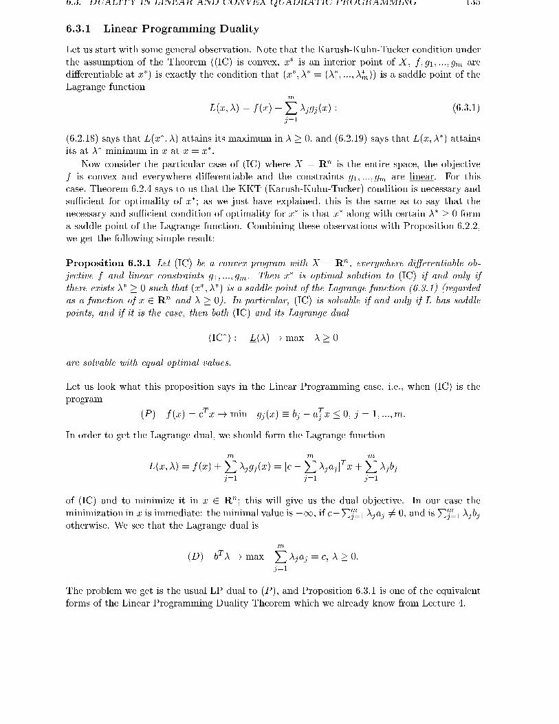
6.3. DUALITY IN LINEAR AND CONVEX QUADRATIC PROGRAMMING 135
6.3.1 Linear Programming Duality
Let us start with some general observation. Note that the Karush-Kuhn-Tucker condition underthe assumption of the Theorem ((IC) is convex, x� is an interior point of X, f; g1; :::; gm aredi�erentiable at x�) is exactly the condition that (x�; �� = (��1; :::; �
�m)) is a saddle point of the
Lagrange function
L(x; �) = f(x) +mXj=1
�jgj(x) : (6.3.1)
(6.2.18) says that L(x�; �) attains its maximum in � � 0, and (6.2.19) says that L(x; ��) attainsits at �� minimum in x at x = x�.
Now consider the particular case of (IC) where X = Rn is the entire space, the objectivef is convex and everywhere di�erentiable and the constraints g1; :::; gm are linear. For thiscase, Theorem 6.2.4 says to us that the KKT (Karush-Kuhn-Tucker) condition is necessary andsuÆcient for optimality of x�; as we just have explained, this is the same as to say that thenecessary and suÆcient condition of optimality for x� is that x� along with certain �� � 0 forma saddle point of the Lagrange function. Combining these observations with Proposition 6.2.2,we get the following simple result:
Proposition 6.3.1 Let (IC) be a convex program with X = Rn, everywhere di�erentiable ob-jective f and linear constraints g1; :::; gm. Then x� is optimal solution to (IC) if and only ifthere exists �� � 0 such that (x�; ��) is a saddle point of the Lagrange function (6.3.1) (regardedas a function of x 2 Rn and � � 0). In particular, (IC) is solvable if and only if L has saddlepoints, and if it is the case, then both (IC) and its Lagrange dual
(IC�) : L(�)! max j � � 0
are solvable with equal optimal values.
Let us look what this proposition says in the Linear Programming case, i.e., when (IC) is theprogram
(P ) f(x) = cTx! min j gj(x) � bj � aTj x � 0; j = 1; :::;m:
In order to get the Lagrange dual, we should form the Lagrange function
L(x; �) = f(x) +mXj=1
�jgj(x) = [c�mXj=1
�jaj ]Tx+
mXj=1
�jbj
of (IC) and to minimize it in x 2 Rn; this will give us the dual objective. In our case theminimization in x is immediate: the minimal value is �1, if c�Pm
j=1 �jaj 6= 0, and isPm
j=1 �jbjotherwise. We see that the Lagrange dual is
(D) bT�! max jmXj=1
�jaj = c; � � 0:
The problem we get is the usual LP dual to (P ), and Proposition 6.3.1 is one of the equivalentforms of the Linear Programming Duality Theorem which we already know from Lecture 4.

136 LECTURE 6. CONVEX PROGRAMMING, DUALITY, SADDLE POINTS
6.3.2 Quadratic Programming Duality
Now consider the case when the original problem is linearly constrained convex quadratic pro-gram
(P ) f(x) =1
2xTDx+ cTx j gj(x) � bj � aTj x � 0; j = 1; :::;m;
where the objective is a strictly convex quadratic form, so that D = DT is positive de�nitematrix: xTDx > 0 whenever x 6= 0. It is convenient to rewrite the constraints in the vector-matrix form
g(x) = b�Ax � 0; b =
0@ b1:::bm
1A ; A =
0@ aT1:::aTm
1A :In order to form the Lagrange dual to (P ) program, we write down the Lagrange function
L(x; �) = f(x) +Pm
j=1 �jgj(x)= cTx+ �T (b�Ax) + 1
2xTDx
= 12x
TDx� [AT�� c]Tx+ bT�
and minimize it in x. Since the function is convex and di�erentiable in x, the minimum, if exists,is given by the Fermat rule
rxL(x; �) = 0;
which in our situation becomesDx = [AT�� c]:
Since D is positive de�nite, it is nonsingular, so that the Fermat equation has a unique solutionwhich is the minimizer of L(�; �); this solution is
x = D�1[AT�� c]:
Substituting the value of x into the expression for the Lagrange function, we get the dualobjective:
L(�) = �1
2[AT�� c]TD�1[AT�� c] + bT�;
and the dual problem is to maximize this objective over the nonnegative orthant. Usually peoplerewrite this dual problem equivalently by introducing additional variables
t = �D�1[AT�� c] [[AT�� c]TD�1[AT�� c] = tTDt];
with this substitution, the dual problem becomes
(D) � 1
2tTDt+ bT�! max j AT�+Dt = c; � � 0:
We see that the dual problem also turns out to be linearly constrained convex quadratic program.Note also that in the case in question feasible problem (P ) automatically is solvable4)
With this observation, we get from Proposition 6.3.1 the following4) since its objective, due to positive de�niteness of D, goes to in�nity as jxj ! 1, and due to the following
general fact:Let (IC) be a feasible program with closed domain X, continuous on X objective and constraints and such thatf(x)!1 as x 2 X \goes to in�nity" (i.e., jxj ! 1). Then (IC) is solvable.You are welcome to prove this simple statement (it is among the exercises accompanying the Lecture)

6.4. SADDLE POINTS 137
Theorem 6.3.1 [Duality Theorem in Quadratic Programming]Let (P ) be feasible quadratic program with positive de�nite symmetric matrix D in the objective.Then both (P ) and (D) are solvable, and the optimal values in the problems are equal to eachother.
The pair (x; (�; t)) of feasible solutions to the problems is comprised of the optimal solutionsto them
(i) if and only if the primal objective at x is equal to the dual objective at (�; t) [\zero dualitygap" optimality condition]same as
(ii) if and only if�i(Ax� b)i = 0; i = 1; :::;m; and t = �x: (6.3.2)
Proof. (i): we know from Proposition 6.3.1 that the optimal value in minimization problem(P ) is equal to the optimal value in the maximization problem (D). It follows that the valueof the primal objective at any primal feasible solution is � the value of the dual objective atany dual feasible solution, and equality is possible if and only if these values coincide with theoptimal values in the problems, as claimed in (i).
(ii): Let us compute the di�erence � between the values of the primal objective at primalfeasible solution x and the dual objective at dual feasible solution (�; t):
� = cTx+ 12x
TDx� [bT�� 12 tTDt]
= [AT�+Dt]Tx+ 12x
TDx+ 12 tTDt� bT�
[since AT�+Dt = c]= �T [Ax� b] + 1
2 [x+ t]TD[x+ t]
Since Ax�b � 0 and � � 0 due to primal feasibility of x and dual feasibility of (�; t), both termsin the resulting expression for � are nonnegative. Thus, � = 0 (which, by (i). is equivalentto optimality of x for (P ) and optimality of (�; t) for (D)) if and only if
Pmj=1 �j(Ax� b)j = 0
and (x+ t)TD(x+ t) = 0. The �rst of these equalities, due to � � 0 and Ax � b, is equivalentto �j(Ax � b)j = 0, j = 1; :::;m; the second, due to positive de�niteness of D, is equivalent tox+ t = 0.
6.4 Saddle Points
6.4.1 De�nition and Game Theory interpretation
When speaking about the "saddle point" formulation of optimality conditions in ConvexProgramming, we touched a very interesting in its own right topic of Saddle Points. Thisnotion is related to the situation as follows. Let X � Rn and � 2 Rm be two nonemptysets, and let
L(x; �) : X � �! R
be a real-valued function of x 2 X and � 2 �. We say that a point (x�; ��) 2 X � � is asaddle point of L on X � �, if L attains in this point its maximum in � 2 � and attains atthe point its minimum in x 2 X :
L(x; ��) � L(x�; ��) � L(x�; �) 8(x; �) 2 X � �: (6.4.1)
The notion of a saddle point admits natural interpretation in game terms. Consider what iscalled a two person zero sum game where player I chooses x 2 X and player II chooses � 2 �;after the players have chosen their decisions, player I pays to player II the sum L(x; �). Of

138 LECTURE 6. CONVEX PROGRAMMING, DUALITY, SADDLE POINTS
course, I is interested to minimize his payment, while II is interested to maximize his income.What is the natural notion of the equilibrium in such a game { what are the choices (x; �)of the players I and II such that every one of the players is not interested to vary his choiceindependently on whether he knows the choice of his opponent? It is immediately seen thatthe equilibria are exactly the saddle points of the cost function L. Indeed, if (x�; ��) is sucha point, than the player I is not interested to pass from x to another choice, given thatII keeps his choice � �xed: the �rst inequality in (6.4.1) shows that such a choice cannotdecrease the payment of I. Similarly, player II is not interested to choose something di�erentfrom ��, given that I keeps his choice x� { such an action cannot increase the income of II.On the other hand, if (x�; ��) is not a saddle point, then either the player I can decreasehis payment passing from x� to another choice, given that II keeps his choice at �� { this isthe case when the �rst inequality in (6.4.1) is violated, or similarly for the player II; thus,equilibria are exactly the saddle points.
The game interpretation of the notion of a saddle point motivates deep insight into thestructure of the set of saddle points. Consider the following two situations:
(A) player I makes his choice �rst, and player II makes his choice already knowing thechoice of I;
(B) vice versa, player II chooses �rst, and I makes his choice already knowing the choiceof II.
In the case (A) the reasoning of I is: If I choose some x, then II of course will choose �which maximizes, for my x, my payment L(x; �), so that I shall pay the sum
L(x) = sup�2�
L(x; �);
Consequently, my policy should be to choose x which minimizes my loss function L, i.e., theone which solves the optimization problem
(I) minx2X
L(x);
with this policy my anticipated payment will be
infx2X
L(x) = infx2X
sup�2�
L(x; �):
In the case (B), similar reasoning of II enforces him to choose � maximizing his pro�tfunction
L(�) = infx2X
L(x; �);
i.e., the one which solves the optimization problem
(II) max�2�
L(�);
with this policy, the anticipated pro�t of II is
sup�2�
L(�) = sup�2�
infx2X
L(x; �):
Note that these two reasonings relate to two di�erent games: the one with priority ofII (when making his decision, II already knows the choice of I), and the one with similarpriority of I. Therefore we should not, generally speaking, expect that the anticipated lossof I in (A) is equal to the anticipated pro�t of II in (B). What can be guessed is that theanticipated loss of I in (B) is less than or equal to the anticipated pro�t of II in (A), sincethe conditions of the game (B) are better for I than those of (A). Thus, we may guess thatindependently of the structure of the function L(x; �), there is the inequality
sup�2�
infx2X
L(x; �) � infx2X
sup�2�
L(x; �): (6.4.2)

6.4. SADDLE POINTS 139
This inequality indeed is true; which is seen from the following reasoning:
8y 2 X : infx2X L(x; �) � L(y; �))8y 2 X : sup�2� infx2X L(x; �) � sup�2� L(y; �) � L(y);
consequently, the quantity sup�2� infx2X L(x; �) is a lower bound for the function L(y),y 2 X , and is therefore a lower bound for the in�mum of the latter function over y 2 X , i.e.,is a lower bound for infy2X sup�2� L(y; �).
Now let us look what happens when the game in question has a saddle point (x�; ��), sothat
L(x; ��) � L(x�; ��) � L(x�; �) 8(x; �) 2 X � �: (6.4.3)
I claim that if it is the case, then
(*) x� is an optimal solution to (I), �� is an optimal solution to (II) and the optimalvalues in these two optimization problems are equal to each other (and are equal to thequantity L(x�; ��)).
Indeed, from (6.4.3) it follows that
L(��) � L(x�; ��) � L(x�);
whence, of course,
sup�2�
L(�) � L(��) � L(x�; ��) � L(x�) � infx2X
L(x):
the very �rst quantity in the latter chain is � the very last quantity by (6.4.2), which ispossible if and only if all the inequalities in the chain are equalities, which is exactly what issaid by (A) and (B).
Thus, if (x�; ��) is a saddle point of L, then (*) takes place. We are about to demonstratethat the inverse also is true:
Theorem 6.4.1 [Structure of the saddle point set] Let L : X � Y ! R be a function.The set of saddle points of the function is nonempty if and only if the related optimizationproblems (I) and (II) are solvable and the optimal values in the problems are equal to eachother. If it is the case, then the saddle points of L are exactly all pairs (x�; ��) with x� beingan optimal solution to (I) and �� being an optimal solution to (II), and the value of the costfunction L(�; �) at every one of these points is equal to the common optimal value in (I) and(II).
Proof. We already have established \half" of the theorem: if there are saddle points of L,then their components are optimal solutions to (I), respectively, (II), and the optimal valuesin these two problems are equal to each other and to the value of L at the saddle point inquestion. To complete the proof, we should demonstrate that if x� is an optimal solutionto (I), �� is an optimal solution to (II) and the optimal values in the problems are equal toeach other, then (x�; ��) is a saddle point of L. This is immediate: we have
L(x; ��) � L(��) [ de�nition of L]= L(x�) [by assumption]� L(x�; �) [de�nition of L]
whenceL(x; ��) � L(x�; �) 8x 2 X;� 2 �;
substituting � = �� in the right hand side of this inequality, we get L(x; ��) � L(x�; ��),and substituting x = x� in the right hand side of our inequality, we get L(x�; ��) � L(x�; �);thus, (x�; ��) indeed is a saddle point of L.

140 LECTURE 6. CONVEX PROGRAMMING, DUALITY, SADDLE POINTS
6.4.2 Existence of saddle points
It is easily seen that a "quite respectable" cost function, say, L(x; �) = (x� �)2 on the unitsquare [0; 1]� [0; 1] has no saddle points. Indeed, here
L(x) = sup�2[0;1]
(x� �)2 = maxfx2; (1� x)2g;
L(�) = infx2[0;1]
(x � �)2 = 0; � 2 [0; 1];
so that the optimal value in (I) is 14 , and the optimal value in (II) is 0; according to Theorem
6.4.1 it means that L has no saddle points.On the other hand, there are generic cases when L has a saddle point, e.g., when
L(x; �) = f(x) +mXi=1
�igi(x) : X �Rm+ ! R
is the Lagrange function of a solvable convex program satisfying the Slater condition. Notethat in this case L is convex in x for every � 2 � � Rm
+ and is linear (and therefore concave)in � for every �xed X . As we shall see in a while, these are the structural properties of Lwhich take upon themselves the \main responsibility" for the fact that in the case in questionthe saddle points exist. Namely, there exists the following
Theorem 6.4.2 [Existence of saddle points of a convex-concave function (Sion-Kakutani)]Let X and � be convex compact sets in Rn and Rm, respectively, and let
L(x; �) : X � �! R
be a continuous function which is convex in x 2 X for every �xed � 2 � and is concave in� 2 � for every �xed x 2 X. Then L has saddle points on X � �.
Proof. According to Theorem 6.4.1, we should prove that
� (i) Optimization problems (I) and (II) are solvable
� (ii) the optimal values in (I) and (II) are equal to each other.
(i) is valid independently of convexity-concavity of L and is given by the following routinereasoning from the Analysis:
Since X and � are compact sets and L is continuous on X � �, due to the well-knownAnalysis theorem L is uniformly continuous on X � �: for every � > 0 there exists Æ(�) > 0such that
jx� x0j+ j�� �0j � Æ(�)) jL(x; �)� L(x0; �0)j � � 5) (6.4.4)
In particular,jx� x0j � Æ(�)) jL(x; �) � L(x0�)j � �;
whence, of course, alsojx� x0j � Æ(�)) jL(x)� L(x0)j � �;
so that the function L is continuous on X . Similarly, L is continuous on �. Taking in accountthat X and � are compact sets, we conclude that the problems (I) and (II) are solvable.
(ii) is the essence of the matter; here, of course, the entire construction heavily exploitsconvexity-concavity of L.
00. To prove (ii), we �rst establish the following statement, which is important by itsown right:
5) for those not too familiar with Analysis, I wish to stress the di�erence between the usual continuity andthe uniform continuity: continuity of L means that given � > 0 and a point (x; �), it is possible to choose Æ > 0such that (6.4.4) is valid; the corresponding Æ may depend on (x; �), not only on �. Uniform continuity meansthat this positive Æ may be chosen as a function of � only. The fact that a continuous on a compact set functionautomatically is uniformly continuous on the set is one of the most useful features of compact sets
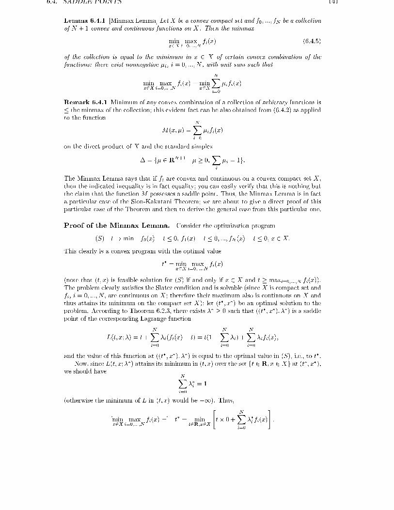
6.4. SADDLE POINTS 141
Lemma 6.4.1 [Minmax Lemma] Let X be a convex compact set and f0; :::; fN be a collectionof N + 1 convex and continuous functions on X. Then the minmax
minx2X
maxi=0;:::;N
fi(x) (6.4.5)
of the collection is equal to the minimum in x 2 X of certain convex combination of thefunctions: there exist nonnegative �i, i = 0; :::; N , with unit sum such that
minx2X
maxi=0;:::;N
fi(x) = minx2X
NXi=0
�ifi(x)
Remark 6.4.1 Minimum of any convex combination of a collection of arbitrary functions is� the minmax of the collection; this evident fact can be also obtained from (6.4.2) as appliedto the function
M(x; �) =NXi=0
�ifi(x)
on the direct product of X and the standard simplex
� = f� 2 RN+1 j � � 0;Xi
�i = 1g:
The Minmax Lemma says that if fi are convex and continuous on a convex compact set X ,then the indicated inequality is in fact equality; you can easily verify that this is nothing butthe claim that the function M possesses a saddle point. Thus, the Minmax Lemma is in facta particular case of the Sion-Kakutani Theorem; we are about to give a direct proof of thisparticular case of the Theorem and then to derive the general case from this particular one.
Proof of the Minmax Lemma. Consider the optimization program
(S) t! min j f0(x)� t � 0; f1(x) � t � 0; :::; fN(x) � t � 0; x 2 X:This clearly is a convex program with the optimal value
t� = minx2X
maxi=0;:::;N
fi(x)
(note that (t; x) is feasible solution for (S) if and only if x 2 X and t � maxi=0;:::;N fi(x)).The problem clearly satis�es the Slater condition and is solvable (since X is compact set andfi, i = 0; :::; N , are continuous on X ; therefore their maximum also is continuous on X andthus attains its minimum on the compact set X); let (t�; x�) be an optimal solution to theproblem. According to Theorem 6.2.3, there exists �� � 0 such that ((t�; x�); ��) is a saddlepoint of the corresponding Lagrange function
L(t; x;�) = t+NXi=0
�i(fi(x) � t) = t(1�NXi=0
�i) +NXi=0
�ifi(x);
and the value of this function at ((t�; x�); ��) is equal to the optimal value in (S), i.e., to t�.Now, since L(t; x;��) attains its minimum in (t; x) over the set ft 2 R; x 2 Xg at (t�; x�),
we should haveNXi=0
��i = 1
(otherwise the minimum of L in (t; x) would be �1). Thus,
[minx2X
maxi=0;:::;N
fi(x) =] t� = mint2R;x2X
"t� 0 +
NXi=0
��i fi(x)
#;
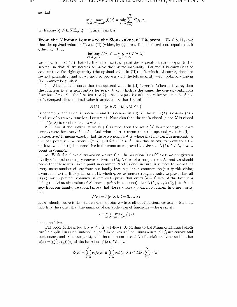
142 LECTURE 6. CONVEX PROGRAMMING, DUALITY, SADDLE POINTS
so that
minx2X
maxi=0;:::;N
fi(x) = minx2X
NXi=0
��i fi(x)
with some ��i � 0;PN
i=0 ��i = 1, as claimed.
From the Minmax Lemma to the Sion-Kakutani Theorem. We should provethat the optimal values in (I) and (II) (which, by (i), are well de�ned reals) are equal to eachother, i.e., that
infx2X
sup�2�
L(x; �) = sup�2�
infx2X
L(x; �):
we know from (6.4.4) that the �rst of these two quantities is greater than or equal to thesecond, so that all we need is to prove the inverse inequality. For me it is convenient toassume that the right quantity (the optimal value in (II)) is 0, which, of course, does notrestrict generality; and all we need to prove is that the left quantity { the optimal value in(I) { cannot be positive.
10. What does it mean that the optimal value in (II) is zero? When it is zero, thenthe function L(�) is nonpositive for every �, or, which is the same, the convex continuousfunction of x 2 X { the function L(x; �) { has nonpositive minimal value over x 2 X . SinceX is compact, this minimal value is achieved, so that the set
X(�) = fx 2 X j L(x; �) � 0gis nonempty; and since X is convex and L is convex in x 2 X , the set X(�) is convex (as alevel set of a convex function, Lecture 4). Note also that the set is closed (since X is closedand L(x; �) is continuous in x 2 X).
20. Thus, if the optimal value in (II) is zero, then the set X(�) is a nonempty convexcompact set for every � 2 �. And what does it mean that the optimal value in (I) isnonpositive? It means exactly that there is a point x 2 X where the function L is nonpositive,i.e., the point x 2 X where L(x; �) � 0 for all � 2 �. In other words, to prove that theoptimal value in (I) is nonpositive is the same as to prove that the sets X(�), � 2 �, have apoint in common.
30. With the above observations we see that the situation is as follows: we are given afamily of closed nonempty convex subsets X(�), � 2 �, of a compact set X , and we shouldprove that these sets have a point in common. To this end, in turn, it suÆces to prove thatevery �nite number of sets from our family have a point in common (to justify this claim,I can refer to the Helley Theorem II, which gives us much stronger result: to prove that allX(�) have a point in common, it suÆces to prove that every (n + 1) sets of this family, nbeing the aÆne dimension of X , have a point in common). Let X(�0); :::; X(�N ) be N + 1sets from our family; we should prove that the sets have a point in common. In other words,let
fi(x) = L(x; �i); i = 0; :::; N ;
all we should prove is that there exists a point x where all our functions are nonpositive, or,which is the same, that the minmax of our collection of functions { the quantity
� � minx2X
maxi=1;:::;N
fi(x)
is nonpositive.The proof of the inequality � � 0 is as follows. According to the Minmax Lemma (which
can be applied in our situation { since L is convex and continuous in x, all fi are convex andcontinuous, and X is compact), � is the minimum in x 2 X of certain convex combination
�(x) =PN
i=0 �ifi(x) of the functions fi(x). We have
�(x) =NXi=0
�ifi(x) �NXi=0
�iL(x; �i) � L(x;NXi=0
�i�i)

6.4. SADDLE POINTS 143
(the last inequality follows from concavity of L in �; this is the only { and crucial { point
where we use this assumption). We see that �(�) is majorated by L(�; �) for a properly chosen�; it follows that the minimum of � in x 2 X { and we already know that this minimum is
exactly � { is nonpositive (recall that the minimum of L in x is nonpositive for every �).

144 LECTURE 6. CONVEX PROGRAMMING, DUALITY, SADDLE POINTS
Assignment # 6 (Lecture 6)
Exercise 6.1 Prove the following statement:Assume that the optimization program
f(x)! min j gj(x) � 0; j = 1; :::;m; hl(x) = 0; l = 1; :::; k; x 2 X � Rn
is feasible, the domain X of the problem is closed, and the functions f; g1; :::; gm; h1; :::; hk arecontinuous on X. Assume, besides this, that the problem is \coercive", i.e., there exists afunction s(t)!1, t!1, on the nonnegative ray such that
maxff(x); g1(x); :::; gm(x); jh1(x)j; :::; jhk(x)jg � s(jxj) 8x 2 X:Prove that under this assumption the problem is solvable.Hint: conisder what is called minimizing sequence fxig, i.e., a sequence of feasible solutions tothe problem with the values of the objective converging, as i!1, to the optimal value of theproblem. Prove that the sequence is bounded and therefore possesses limiting points; vewrifythat every such point is an optimal solution to the problem.
Exercise 6.2 Find the minimizer of a linear function
f(x) = cTx
on the set
Vp = fx 2 Rn jnXi=1
jxijp � 1g;
here p, 1 < p <1, is a parameter.
Exercise 6.3 Cosider the function
I(u; v) =kXi=1
ui ln(ui=vi)
regarded as a function of nonnegative u 2 Rk and positive v 2 Rk; here 0 ln 0 = 0.1) Prove that the function is convex in (u; v) on the indicated set2) Prove that if u; v 2 � = fz 2 Rk
+ :P
i zi = 1g and u � 0, then
I(u; v) � 0;
with the inequality being strict provided that u 6= v.Hint: apply Jensen's inequality to the strictly convex on (0;1) function � ln tComment: vector z 2 � can be regarded as probability distribution on k-point set: zi is theprobability assigned to ith element of the set. With this interpretation, I(u; v) is a kind of\directed distance" between probability distributions: it sets into correspondence to an orderedpair of distributions certain nonnegative real which is positive whenever the distributions aredistinct, and is zero otherwise. This quantity is called the Kullback distance (this is not adistance in the standard de�nition, since it is not symmetric: I(u; v) is not the same as I(v; u)).The Kullback distance between distributions plays important role in the Theory of StatisticalDecisions (see example in Exercise 6.6).
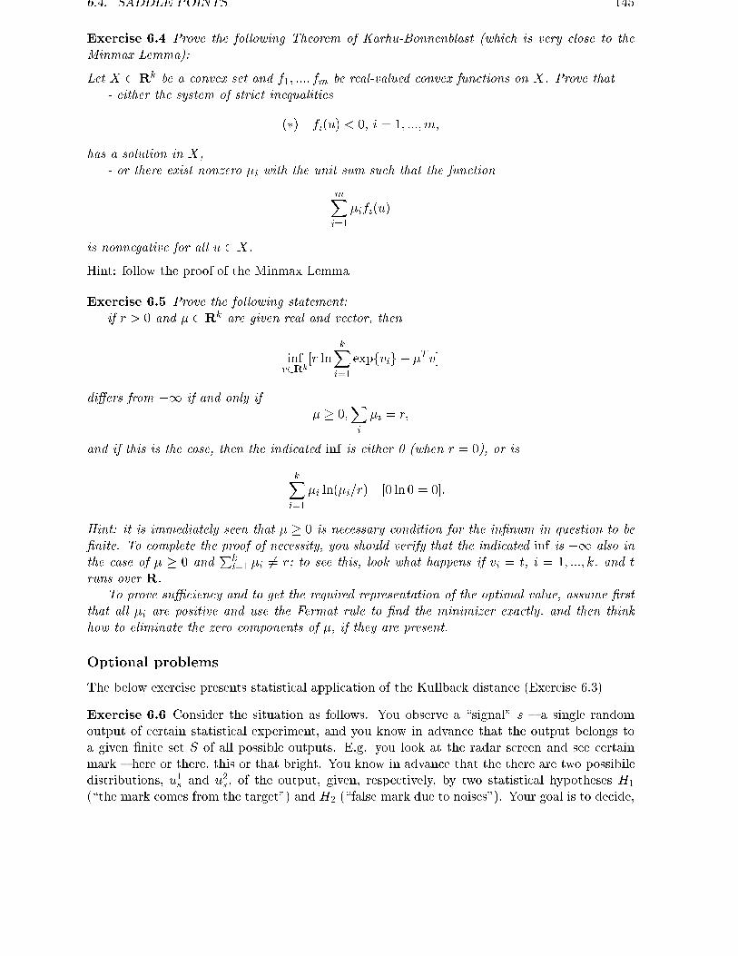
6.4. SADDLE POINTS 145
Exercise 6.4 Prove the following Theorem of Karhu-Bonnenblast (which is very close to theMinmax Lemma):
Let X � Rk be a convex set and f1; :::; fm be real-valued convex functions on X. Prove that- either the system of strict inequalities
(�) fi(u) < 0; i = 1; :::;m;
has a solution in X,- or there exist nonzero �i with the unit sum such that the function
mXi=1
�ifi(u)
is nonnegative for all u 2 X.
Hint: follow the proof of the Minmax Lemma
Exercise 6.5 Prove the following statement:if r > 0 and � 2 Rk are given real and vector, then
infv2Rk
[r lnkXi=1
expfvig � �T v]
di�ers from �1 if and only if� � 0;
Xi
�i = r;
and if this is the case, then the indicated inf is either 0 (when r = 0), or is
�kXi=1
�i ln(�i=r) [0 ln 0 = 0]:
Hint: it is immediately seen that � � 0 is necessary condition for the in�num in question to be�nite. To complete the proof of necessity, you should verify that the indicated inf is �1 also inthe case of � � 0 and
Pki=1 �i 6= r; to see this, look what happens if vi = t, i = 1; :::; k, and t
runs over R.To prove suÆciency and to get the required representation of the optimal value, assume �rst
that all �i are positive and use the Fermat rule to �nd the minimizer exactly, and then thinkhow to eliminate the zero components of �, if they are present.
Optional problems
The below exercise presents statistical application of the Kullback distance (Exercise 6.3)
Exercise 6.6 Consider the situation as follows. You observe a \signal" s { a single randomoutput of certain statistical experiment, and you know in advance that the output belongs toa given �nite set S of all possible outputs. E.g. you look at the radar screen and see certainmark { here or there, this or that bright. You know in advance that the there are two possibiledistributions, u1s and u2s, of the output, given, respectively, by two statistical hypotheses H1
(\the mark comes from the target") and H2 (\false mark due to noises"). Your goal is to decide,

146 LECTURE 6. CONVEX PROGRAMMING, DUALITY, SADDLE POINTS
given the observation, which of these hypotheses is valid. The only deterministic policy youcould use is as follows: partition in advance the set of all tentative outputs S into two non-overlapping subsets S1 and S2, and check whether the observed s belongs to S1 or to S2; in the�rst case you claim that the signal comes from the hypothesis H1, in the second { that it comesfrom H2. If every output can be obtained, with positive probability, from both the hypotheses,you clearly cannot �nd a 100% reliable decision rule (� partitioning S = S1 [ S2); what we canspeak about are the probabilities of errors
�1 =Xs2S2
u1s
(\missing" probability { the mark came from the target and you decided that it came fromnoise), and
�2 =Xs2S1
u2s
(\false alarm" probability { you decided that the mark came from the target when it came fromnoise).
We would be interested to make both p1 and p2 small. A very natural (and an extremelyimportant) question here is what are the lower bounds on the errors. A simple answer is givenby the following necessary condition (which in many cases turns out to be \sharp"):
if �, � are two given positive reals less than 1/2 each, then a decision rule which ensures �1 � �and �2 � � exists only if the Kullback distance from the distribution u1 to the distribution u2 isnot too small, namely,
I(u1; u2) � (1� �) ln�1� �
�
�+ � ln
��
1� �
�:
The exercise is to prove the necessity of the indicated condition.
Remark 6.4.2 Both the Kullback distance and the indicated necessary condition have contin-uous analogies. Namely, the Kullback distance between two distributions on Rl with densities,respectively, v1(x), v2(x), is de�ned as
I(v1; v2) =Zv1(x) ln(v1(x)=v2(x))dx
(\directed distance" from v1 to v2), and with this de�nition of the distance the indicated neces-sary condition remains valid for continuous random signals.
Note that for Gaussian distributions v1 and v2 with the unit covariance matrix and the meanvalues m1, m2 the Kullback distance is simply
k m1 �m2 k22 :
Lecture 7
Optimality Conditions
This Lecture, the last one in the theoretical part of the course, is devoted to optimality conditionsin general-type Mathematical Programming programs
(P ) f(x)! min j g(x) � (g1(x); g2(x); :::; gm(x)) � 0; h(x) = (h1(x); :::; hk(x)) = 0; x 2 X:
The question we are interested in is as follows:
� Assume that we are given a feasible solution x� to (P ). What are the conditions (necessary,suÆcient, necessary and suÆcient) for x� to be optimal?
We, as it is normally the case in Mathematical Programming, intend to answer this questionunder the following assumptions on the data:
� A. x� is an interior point of the domain of the problem X;
� B. The functions f; g1; :::; gm; h1; :::; hk are smooth at x� (at least once continuously di�er-entiable in a neighbourhood of the point; when necessary, we shall require more smooth-ness)
Let me stress that we are not going to impose on the problem structural assumptions likeconvexity, in contrast to what was done in the previous Lecture.
Before coming to \technical" considerations, let us discuss the following \philosophical"questions:
� Conditions of what kind are we interested in?
� Why are we interested in these conditions?
The answer to the �rst question is as follows: we are interested in local and veri�able optimalityconditions. Locality means that the conditions should be expressed in terms of local propertiesof the data { in terms of the values and derivatives (of �rst, second,... order) of the functionsf; g1; :::; gm; h1; :::; hk at x�. Veri�ability means that given the values and the derivatives of theindicated functions at x�, we should be able to verify eÆciently whether the condition is or isnot satis�ed.
The outlined { quite reasonable { requirements to the conditions to be derived lead to ratherunpleasant consequences:
147

148 LECTURE 7. OPTIMALITY CONDITIONS
What we may hope for are necessary conditions for optimality of x� and suÆcientconditions for local optimality of x�, and not suÆcient conditions for global optimal-ity of x�.
Let me explain, �rst, what is meant in the above claim { what does it mean \local" and \global"optimality, and, second, why the claim is true.
Global optimality of x� is nothing but the actual optimality: x� is a feasible solution to (P )with the best possible value of the objective { the one which is � the value of the objective atany other feasible solution to the problem. In contrast to this, local optimality of x� means thatx� is feasible solution which is not worse, from the viewpoint of the values of the objective, thanother feasible solutions close enough to x�. The formal de�nition is as follows:
A feasible solution x� to (P ) is called locally optimal, if there exists a neighbourhood U ofx� such that x� is optimal solution of the \restricted to U" version of (P ), i.e., if
x 2 U; g(x) � 0; h(x) = 0) f(x) � f(x�):
(note that in the last relation I skip the inclusion x 2 X in the premise of the implication; thisis because we have assumed that x� is an interior point of X, so that shrinking, if necessary,U , we always can make it part of X and thus make the inclusion x 2 X a consequence of theinclusion x 2 U).
In the convex case local optimality is the same as the global one (this follows from Theorem5.5.1 combined with the fact that the feasible set of a convex program is convex). In the generalcase these two notions are di�erent { a globally optimal solution is, of course, a locally optimalone, but not vice versa: look at something like the problem
f(x) = 0:1x2 + sin2 x! min;
here all points xk = �k are local minimizers of the objective, but only one of them { 0 { is itsglobal minimizer.
Note that since a globally optimal solution for sure is a locally optimal one, the necessarycondition for local optimality (and these are all necessary optimality conditions to be discussed)are necessary for global optimality as well.
Now, why it is true that in the general case it is impossible to point out local suÆcientcondition for global optimality, it also is clear: because local information on a function f at alocal minimizer x� of the function does not allow to understand that the minimizer is only localand not a global one. Indeed, let us take the above f and x� = �; this is only local, not global,minimizer of f . At the same time we can easily change f outside a neighbourhood of x� andmake x� the global minimizer of the updated function (draw the graph of f to see it). Note thatwe can easily make the updated function �f as smooth as we wish. Now, local information { valueand derivatives at x� { on f and on the updated function �f are the same, since the functionscoincide with each other in a neighbourhood of x�. It follows that there is no test which takeson input local information on the problem at x� and correctly reports on output whether x� isor is not a global minimizer of the objective, even if we assume the objective to be very smooth.Indeed, such a test is unable to distinguish the above f and �f and is therefore enforced, beingasked once about f and once about �f , report both times the same answer; whatever is theanswer, in one of these two cases it is false!
The diÆculty we have outlined is intrinsic for nonconvex optimization: not only there doesnot exist \eÆcient local test" for global optimality; there also does not exist, as we shall see in

149
our forthcoming lectures, an eÆcient algorithm capable to approximate global minimizer of ageneral-type Mathematical Programming problem, even one with very smooth data.
In view of this unpleasant and unavoidable feature of general-type Mathematical Program-ming problems, the answer to the second of the outlined questions { what for we use Optimalityconditions in Mathematical Programming { is not as optimistic as we would wish it to be. Asfar as conditions for global optimality are concerned, we may hope for necessary optimalityconditions only; in other words, we may hope for a test which is capable to say that what wehave is not a globally optimal solution. Since there is no (local) suÆcient condition for globaloptimality, we have no hope to design a local test capable to say that what we have is the\actual" { global { solution to the problem. The best we may hope for in this direction is asuÆcient condition for local optimality, i.e., a local test capable to say that what we have cannotbe improved by small modi�cations.
The pessimism caused by the above remarks has, however, its bounds. A necessary optimalitycondition is certain relation which must be satis�ed at optimal solution. If we are clever enoughto generate { on paper or algorithmically { all candidates x� which satisfy this relation, andif the list of these candidates turns out to be �nite, then we may hope that looking throughthe list and choosing in it the best, from the viewpoint of the objective, feasible solution, weeventually shall �nd the globally optimal solution (given that it exists). Needless to say, theoutlined possibility is met only in \simple particular cases", but already these cases sometimesare extremely important (we shall discuss an example of this type at the end of this Lecture).Another way to utilize necessary and/or suÆcient conditions for local optimality is to use themas \driving force" in optimization algorithms. Here we generate a sequence of approximatesolutions and subject them to the test for local optimality given by our optimality condition. Ifthe current iterate passes the test, we terminate with a locally optimal solution to the problem; ifit is not the case, then the optimality condition (which is violated at the current iterate) normallysays to us how to update the iterate in order to reduce \violation" of the condition. As a result ofthese sequential updatings, we get a sequence of iterates which, under reasonable assumptions,can be proved to converge to a locally optimal solution to the problem. As we shall see in theforthcoming lectures, this idea underlies all traditional computational methods of MathematicalProgramming. Of course, with this scheme it in principle is impossible to guarantee convergenceto globally optimal solution (imagine that we start at a locally optimal solution which is not aglobally optimal one; with the outlined scheme, we shall terminate immediately!) Although thisis a severe drawback of the scheme, it does not kill the traditional \optimality-conditions-based"methods. First, it may happen that we are lucky and there are no \false" local solutions { theonly local solution is the global one; then the above scheme will approximate the actual solution(although we never will know that it is the case...) Second, in many practical situations we areinterested in improving a given initial solution to the problem rather than in �nding the \bestpossible" solution, and the traditional methods normally allow to achieve this restricted goal.
Now let us pass from the \motivation preamble" to the mathematics of optimality conditions.There are two kinds of them { conditions utilizing the �rst-order information of the objectiveand the constraints at x� only (the values and the gradients of these functions), and second-orderconditions using the second order derivatives as well. As we shall see, all �rst-order optimalityconditions are only necessary for optimality. Among the second-order optimality conditions,there are both necessary and suÆcient for local optimality.

150 LECTURE 7. OPTIMALITY CONDITIONS
7.1 First Order Optimality Conditions
The idea of the �rst order optimality conditions is extremely simple. Consider an optimizationproblem (P ), and let x� be a feasible solution to the problem. To derive a necessary conditionfor local optimality of x� is the same as to �nd a consequence of the fact that x� is locallyoptimal; such a consequence is, of course, a necessary optimality condition. Thus, assume thatx� is locally optimal for (P ), and let us try to guess what can be derived from this fact. Themost straightforward idea is as follows: let us approximate the objective and the constraintsof the actual problem (P ) in a neighbourhood of x� by \simple" functions, thus coming to\approximating problem" ( bP ). We may hope that if the approximation is good enough, thatthe local property of (P ) we are interested in { the property that x� is a locally optimal solutionto (P ) { will be inherited by ( bP ). If
� (A) ( bP ) is that simple that we can say \constructively" what does it mean that x� islocally optimal for ( bP ),and
� (B) we can prove that our hypothesis
\if x� is locally optimal for (P ), it is locally optimal for ( bP ) as well"is true,
then the condition given by (A) will be necessary for local optimality of x� in (P ).There is, basically, only one natural way to implement this idea, given that we are interested
in the �rst order optimality conditions and, consequently, that bP ) should be posed in terms ofthe values and the gradients of the original objective and constraints at x� only. This way is tolinearize the original objective and constraints at x� and to make the resulting aÆne functionsthe objective and the constraints of ( bP ). The linearizations in question are
�f(x) = f(x�) + (x� x�)Trf(x�);�gi(x) = gi(x�) + (x� x�)Trgi(x�); i = 1; :::;m;�hi(x) = hi(x�) + (x� x�)Trhj(x�); j = 1; :::; k;
which results in the Linear Programming problem ( bP ):( bP ) :min f(x�) + (x� x�)Trf(x�)s.t.
gi(x�) + (x� x�)Trgi(x�) � 0; i = 1; :::;m(x� x�)Trhj(x�) = 0; j = 1; :::; k
(I omit hj(x�) { they are zeros, since x� is feasible).Now, when x� is an optimal solution to the LP program ( bP ), it is said by the Linear Pro-
gramming Duality Theorem. Since we have not established the theorem for the particular formof the LP program we are interested in (the one with equality constraints and not inequalityconstraints only), it makes sense to derive the required optimality condition explicitly from thesource of the LP Duality Theorem { from the Homogeneous Farkas Lemma.

7.1. FIRST ORDER OPTIMALITY CONDITIONS 151
Assume that x� (which is clearly feasible for ( bP ) { recall that x� is feasible for (P )) isoptimal for ( bP ). Let I(x�) be the set of indices of all inequality constraints of (P ) which areactive (satis�ed as equalities) at x�, and consider the set
K = fd j dTrgi(x�) � 0; i 2 I(x�); dTrhj(x�) = 0; j = 1; :::; kg:It is absolutely clear that if d 2 K, then all vectors xt = x� + td corresponding to small enoughpositive t are feasible for ( bP ). Since x� is optimal for the latter problem, we should have
f(x�) + (xt � x�)Trf(x�) � f(x�)
for the indicated t, whence dTrf(x�) � 0. Thus,
(*) if x� is optimal for ( bP ), then dTrf(x�) � 0 for all d 2 K;
in fact \if ... then ..." here can be replaced with \if and only if" (why?).Now, by the Homogeneous Farkas Lemma (Lecture 3) statement (*), in turn, is equivalent
to the possibility of representation
rf(x�) = � Xi2I(x�)
��irgj(x�)�kX
j=1
�jrhj(x�) (7.1.1)
with some nonnegative ��i and some real ��j . To see it, note that K is exactly the polyhedralcone
fd j dTrgi(x�) � 0; i 2 I(x�); dTrhj(x�) � 0; dT (�rhj(x�)) � 0; j = 1; :::; kg;and (*) says that the vector rf(x�) has nonnegative inner products with all vectors from K,i.e., with all vectors which have nonnegative inner products with the vectors from the �nite set
A = f�rgi(x�); i 2 I(x�);�rhj(x�); j = 1; :::; kg:By the Homogeneous Farkas Lemma this is the case if and only if rf(x�) is combination withnonnegative coeÆcients of the vectors from A:
rf(x�) = � Xi2I(x�)
��irgi(x�) +kX
j=1
[��j;+ � ��j;j]rhj(x�)
with nonnegative ��j ; ��j;+; �
�j;�. And to say that rf(x�) is representable in the latter form is
the same as to say that it is representable as required in (7.1.1).Now, ��i to the moment are de�ned for i 2 I(x�) only. We loose nothing when de�ning ��i = 0
for i 62 I(x�) and treating the right hand side sum in (7.1.1) as the sum over all i = 1; :::;m.Note also that now we have the complementary slackness relations ��i gi(x
�) = 0, i = 1; :::;m.We have established the following conditional statement:
Proposition 7.1.1 Let x� be locally optimal for (P ) and such that the hypothesis (B) takesplace: x� remains optimal property also for the linearized LP program ( bP ). Then there existnonnegative ��i and real ��j such that
��i gi(x�) = 0; i = 1; :::;m [complementary slackness]
rf(x�) +Pmi=1 �
�irgi(x�) +
Pkj=1 �
�jrhj(x�) = 0 [Euler's Equation]
(7.1.2)

152 LECTURE 7. OPTIMALITY CONDITIONS
The property of x� to be feasible for (P ) and to satisfy the condition \there exist nonnegative��i and real ��j such that ..." from the above Proposition is called the Karush-Kuhn-TuckerOptimality Condition; we already know the version of this condition related to the case ofinequality constrained problems. The point x� which satis�es the KKT Optimality Conditionis called a KKT point of (P ) (sometimes this name is used for the pair (x�;��; ��), i.e., for thepoint x� along with the certi�cate that it satis�es the KKT condition).
From the above discussion it follows that all we may hope for is that the KKT conditionis necessary for local optimality of x�; Proposition 7.1.2 says that this indeed is the case, butunder implicit additional assumption \x� remains...". The problem, consequently, is to convertthis implicit assumption into something veri�able or to eliminate the assumption at all. Thelatter, unfortunately, is impossible, as it is seen from the following elementary example (wherethe problem is even convex):
f(x) � x! min j g1(x) � x2 � 0:
The optimal solution to the problem (in fact { the only feasible solution to it) is x� = 0.However, x� = 0 is not a KKT point of the problem { it is impossible to �nd nonnegative��1 such that
rf(0) + ��1rg1(0) � 1 + ��1 � 0 = 0:
Thus, we indeed need some \regularity assumption" to make the KKT Optimality Conditionnecessary for local optimality. The most general regularity assumption of this type is called\Quali�cation of Constraints". Let us look what does it mean.
Quali�cation of constraints actually says that the feasible set of the actual problem (P )should approximate the feasible set of the linearized problem ( bP ) in a neighbourhood of x�
\up to the highest-order terms in jx � x�j", similarly to what is the case with the data of theproblems. To give the precise de�nition, let us agree to write
�(t) = o(ts)
(� is a function on the nonnegative ray, s > 0), if �(t)t�s ! 0 as t ! +0 and �(0) = 0; this isone of standard Calculus conventions. And we say that problem (P ) satis�es the Quali�cationof Constraints property at feasible solution x�, if there exists function �(t) = o(t) such that
for every feasible solution x to the linearized problem ( bP ) there exists a feasiblesolution x0 to the actual problem (P ) such that
jx� x0j � �(jx� x�j){ the distance between x and x0 goes to zero faster than the distance from x to x�
as x! x�.
The Quali�cation of Constraints condition roughly speaking says that the feasible set of thelinearized problem ( bP ) cannot be (locally, of course) \much wider" than the feasible set of (P ):for every x close to x� and feasible for ( bP ) there exists x0 \very close" to x and feasible for (P ).Note that in the above \bad example" the situation is opposite: the feasible set of ( bP ) is theentire axis (since the constraint in the linearized problem is 0�x � 0), which is a \much wider"set, even locally, than the feasible set f0g of (P ).
It is easily seen that under the Quali�cation of Constraints assumption local optimality ofx� for (P ) implies global optimality of x� for ( bP ), so that this assumption makes the KKTOptimality condition necessary for optimality:

7.1. FIRST ORDER OPTIMALITY CONDITIONS 153
Proposition 7.1.2 Let x� be locally optimal for (P ) and let (P ) satisfy the Quali�cation ofConstraint assumption at x�. Then x� is optimal for ( bP ) nd, consequently, is a KKT point of(P ).
Proof. Let x� be locally optimal for (P ) and let the Quali�cation of Constraints take place; weshould prove that then x� is optimal for ( bP ). Assume, on contrary, that x� is not optimal for( bP ). Since x� clearly is feasible for ( bP ), non-optimality of x� for the latter problem means thatthere exists a feasible solution �x to ( bP ) with less value of the linearized objective f(x�) + (x�x�)Trf(x�) than the value of this objective at x�. Setting d = �x� x�, we therefore obtain
dTrf(x�) < 0:
Now letxt = x� + t(�x� x�); 0 � t � 1:
The points xt are convex combinations of two feasible solutions to ( bP ) and therefore also arefeasible solutions to the latter problem (it is an LP program!) By Quali�cation of Constraints,there exist feasible solutions x0t to the actual problem (P ) such that
jxt � x0tj � �(jxt � x�j) = �(tj�x� x�j) � �(tq); q = j�x� x�j; (7.1.3)
with �(t) = o(t). Now, f is continuously di�erentiable in a neighbourhood of x� (this is our oncefor ever assumption made in the beginning of the Lecture). It follows { this is a well-known factfrom Analysis (an immediate consequence of the Lagrange Mean Value Theorem) { that f islocally Lipschitz continuous at x�: there exists a neighbourhood U of x� and a constant C <1such that
jf(x)� f(y)j � Cjx� yj; x; y 2 U: (7.1.4)
As t! +0, we have xt ! x�, and since jx0t � xtj � �(tq)! 0; t! 0, x0t also converges to x� as
t ! 0; in particular, both xt and x0t belong to U for all small enough positive t. Besides this,from local optimality of x� and the fact that x0t converges to x
� as t ! +0 and is feasible for(P ) for all t we conclude that
f(x0t) � f(x�)
for all small enough positive t. It follows that for small positive t we have
0 � t�1[f(x0t)� f(x�)]� t�1[f(xt)� f(x�)] + t�1[f(x0t)� f(xt)]� t�1[f(xt)� f(x�)] + t�1Cjx0t � xtj [see (7.1.4)]� t�1[f(xt)� f(x�)] + t�1C�(tq) [see (7.1.3)]
= f(x�+td)�f(x�)t + t�1C�(tq):
As t! 0, the last expression in the chain tends to dTrf(x�) < 0 (since �(tq) = o(t)), while thechain itself says that the expression is nonnegative. This is the desired contradiction.
Proposition 7.1.2 is very close to tautology: the question was when the KKT condition isnecessary for local optimality, and the answer we have now { that it for sure is the case when(P ) satis�es the Quali�cation of Constraints assumption at x�. If we can gain something fromthis answer, this something is indeed very small { we do not know how to certify that theQuali�cation of Constraints takes place. There is one trivial case { the one when the constraintsof (P ) are linear; in this case the feasible set of the linearized problem is even not close, but

154 LECTURE 7. OPTIMALITY CONDITIONS
simply coincides with the feasible set of the actual problem (in fact it suÆces to assume linearityof the active at x� constraints only; then the feasible sets of (P ) and ( bP ) coincide with eachother in a neighbourhood of x�, which is quite suÆcient for Constraint Quali�cation).
Among the more general certi�cates { suÆcient conditions { for the Quali�cation of Con-straints 1) the most frequently used is the assumption of regularity of x� for (P ), which is theproperty as follows:
(Regularity):the set comprised of the gradients of all active at x� constraints of (P ) is a linearlyindependent set(recall that a constraint is active at x� if it is satis�ed at this point as equality; inparticular, all equality constraints are active at every feasible solution).
Why (Regularity) implies Quali�cation of Constraints, it becomes clear from the following fun-damental theorem of Analysis (this is one of the forms of the Implicit Function Theorem):
Theorem 7.1.1 Let x� be a point from Rn and �1; :::; �l be k � 1 times continuously di�er-entiable in a neighbourhood of x� functions which are equal to 0 at x� and are such that theirgradients r�i(x�) at x�, i = 1; :::; l, form a linearly independent set.
Then there exists k times continuously di�erentiable along with its inverse substitution ofargument
x = S(y)
which makes all the functions the coordinate ones, i.e. there exists
� a neighbourhood X of the point x� in Rn
� a neighbourhood Y of the origin in Rn
� a one-to-one mapping y 7! S(y) of Y onto X which maps y = 0 to x�: S(0) = x�
{ such that
� (I) S is k times continuously di�erentiable in Y , and its inverse S�1(x) is k times contin-uously di�erentiable in X;
� (ii) the functions
i(y) � �i(S(y))
in Y are just the coordinate functions yi, i = 1; :::; l.
Corollary 7.1.1 Let x�; �1; :::; �l satisfy the premise of Theorem 7.1.1, let q � l, let X be theneighbourhood of x� given by the Theorem, and let � be the solution set of the system
�i(x) � 0; i = 1; :::; q; �i(x) = 0; i = q + 1; :::; l:
1)look how strange is what we are doing { we are discussing suÆcient condition for something { namely, theQuali�cation of Constraints { which in turn is nothing but a suÆcient condition to make something third { theKKT { necessary condition for local optimality. There indeed is something in human being, if he/she is capableto understand these \conditions for conditions" and to operate them!

7.1. FIRST ORDER OPTIMALITY CONDITIONS 155
Then there exists a neighbourhood U � X of x� such that the distance from a point x 2 U to �is bounded from above by constant times the norm of the \violation vector"
Æ(x) =
0BBBBBBB@
maxf�(x); 0g:::
maxf�q(x); 0gj�q+1(x)j
:::j�l(x)j
1CCCCCCCA ;
i.e., there exists a constant D <1 such that for every x 2 U there exists x0 2 � with
jx� x0j � DjÆ(x)j: (7.1.5)
Proof. Let V be a closed ball of positive radius r which is centered at the origin and is containedin Y . Since S is at least once continuously di�erentiable in a neighbourhood of the compact setV , its �rst order derivatives are bounded in V and therefore S is Lipschitz continuous in V withcertain constant D > 0:
jS(y0)� S(y00)j � Djy0 � y00j 8y0; y00 2 V:
Since S�1 is continuous and S�1(x�) = 0, there exists a neighbourhood U � X of x� such thatS�1 maps this neighbourhood into V .
Now let x 2 U , and consider the vector y = S�1(x). Due to the origin of U , this vectorbelongs to V , and due to the origin of S, the �rst l coordinates of the vector are exactly �i(x),i = 1; :::; l (since x = S(y), and we know that �i(S(y)) = yi, i = 1; :::; l). Now consider thevector y0 with the coordinates
y0i =
8<:minfyi; 0g; i = 1; :::; q0; i = q + 1; :::; lyi; i = l + 1; :::; n
:
It is absolutely clear that
� (a) jy0j � jyj, so that y0 2 V along with y;
� (b) the �rst l entries in the vector y0� y form the violation vector Æ(x), and the remainingentries in y0 � y are zero, so that jy0 � yj = jÆ(x)j.
Now let us set x0 = S(y0). Since the �rst l coordinates of y0 = S�1(x0) are exactly �i(x0),i = 1; :::; l, we see that the values of �1; :::; �q at x0 are nonpositive, and the values of theremaining �'s are zero, so that x0 2 �. On the other hand,
jx� x0j � jS(y)� S(y0)j � Djy � y0j = DjÆ(x)j
(we have used the Lipschitz continuity of S in V ), as required.
First Order Optimality Conditions. Now we are able to reach the �rst of our two targets{ to get the First Order Optimality Conditions.
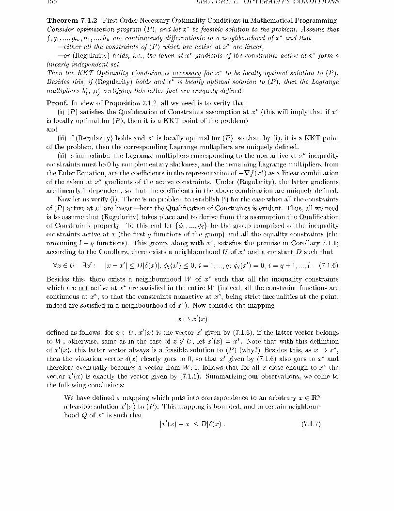
156 LECTURE 7. OPTIMALITY CONDITIONS
Theorem 7.1.2 [First Order Necessary Optimality Conditions in Mathematical Programming]Consider optimization program (P ), and let x� be feasible solution to the problem. Assume thatf; g1; :::; gm; h1; :::; hk are continuously di�erentiable in a neighbourhood of x� and that
{ either all the constraints of (P ) which are active at x� are linear,{ or (Regularity) holds, i.e., the taken at x� gradients of the constraints active at x� form a
linearly independent set.Then the KKT Optimality Condition is necessary for x� to be locally optimal solution to (P ).Besides this, if (Regularity) holds and x� is locally optimal solution to (P ), then the Lagrangemultipliers ��i , �
�j certifying this latter fact are uniquely de�ned.
Proof. In view of Proposition 7.1.2, all we need is to verify that(i) (P ) satis�es the Quali�cation of Constraints assumption at x� (this will imply that if x�
is locally optimal for (P ), then it is a KKT point of the problem)and
(ii) if (Regularity) holds and x� is locally optimal for (P ), so that, by (i), it is a KKT pointof the problem, then the corresponding Lagrange multipliers are uniquely de�ned.
(ii) is immediate: the Lagrange multipliers corresponding to the non-active at x� inequalityconstraints must be 0 by complementary slackness, and the remaining Lagrange multipliers, fromthe Euler Equation, are the coeÆcients in the representation of �rf(x�) as a linear combinationof the taken at x� gradients of the active constraints. Under (Regularity), the latter gradientsare linearly independent, so that the coeÆcients in the above combination are uniquely de�ned.
Now let us verify (i). There is no problem to establish (i) for the case when all the constraintsof (P ) active at x� are linear { here the Quali�cation of Constraints is evident. Thus, all we needis to assume that (Regularity) takes place and to derive from this assumption the Quali�cationof Constraints property. To this end let f�1; :::; �lg be the group comprised of the inequalityconstraints active at x (the �rst q functions of the group) and all the equality constraints (theremaining l � q functions). This group, along with x�, satis�es the premise in Corollary 7.1.1;according to the Corollary, there exists a neighbourhood U of x� and a constant D such that
8x 2 U 9x0 : jx� x0j � DjÆ(x)j; �i(x0) � 0; i = 1; :::; q; �i(x0) = 0; i = q + 1; :::; l: (7.1.6)
Besides this, there exists a neighbourhood W of x� such that all the inequality constraintswhich are not active at x� are satis�ed in the entire W (indeed, all the constraint functions arecontinuous at x�, so that the constraints nonactive at x�, being strict inequalities at the point,indeed are satis�ed in a neighbourhood of x�). Now consider the mapping
x 7! x0(x)
de�ned as follows: for x 2 U , x0(x) is the vector x0 given by (7.1.6), if the latter vector belongsto W ; otherwise, same as in the case of x 62 U , let x0(x) = x�. Note that with this de�nitionof x0(x), this latter vector always is a feasible solution to (P ) (why?) Besides this, as x ! x�,then the violation vector Æ(x) clearly goes to 0, so that x0 given by (7.1.6) also goes to x� andtherefore eventually becomes a vector from W ; it follows that for all x close enough to x� thevector x0(x) is exactly the vector given by (7.1.6). Summarizing our observations, we come tothe following conclusions:
We have de�ned a mapping which puts into correspondence to an arbitrary x 2 Rn
a feasible solution x0(x) to (P ). This mapping is bounded, and in certain neighbour-hood Q of x� is such that
jx0(x)� xj � DjÆ(x)j: (7.1.7)

7.2. SECOND ORDER OPTIMALITY CONDITIONS 157
Now assume that x is a feasible solution to the linearized problem ( bP ). Note that the vector�(x) = (�1(x); :::; �l(x)) admits the representation
�(x) = �lin(x) + �rem(x);
where �lin comes from the linearizations of the functions �i at x� { i.e., from the constraintfunctions of ( bP ), and �rem comes from the remainders in the �rst order Taylor expansions of�i at x�. Since x is feasible for ( bP ), the �rst q entries of �lin(x) clearly are nonpositive, andremaining entries are equal to 0. It follows that if x is feasible for ( bP ), then the norm of theviolation vector Æ(x) does not exceed the norm of the vector �rem(x) (look at the de�nition ofthe violation vector), and the latter norm is � �(jx� x�j) with certain �(t) = o(t); indeed, theremainders in the �rst order Taylor expansions of continuously di�erentiable in a neighbourhoodof x� constraint functions are o(jx�x�j), x being the point where the remainders are evaluated.Combining this observation with (7.1.7), we conclude that there is a neighbourhood Z of x�
such that if x 2 Z is feasible for ( bP ), thenjx0(x)� xj � DjÆ(x)j � Dj�rem(x)j � D�(jx� x�j) (7.1.8)
with some �(t) = o(t). Outside Z the left hand side in the latter equation clearly is boundedfrom above by D0jx� x�j for some D0 (recall that x0(x) is bounded), so that, rede�ning �(t) inan appropriate manner outside a neighbourhood of t = 0, we can ensure that (7.1.8) is valid forall x feasible for ( bP ). Since x0(x), by construction, is feasible for (P ), (7.1.8) demonstrates thatthe Quali�cation of Constraints does hold.
7.2 Second Order Optimality Conditions
A weak point of the �rst order optimality conditions is that they at best are only necessary,but not suÆcient, for local optimality. Indeed, look at the simplest of these conditions, the onefor smooth unconstrained minimization: the Fermat rule rf(x�) = 0. This condition does notdistinguish between local minima, local maxima and \saddle points" (local minimum in somedirections and local maximum in other directions) and therefore de�nitely is not suÆcient forlocal optimality (excluding the case when we preassume convexity of f). It follows that if weare interested in suÆcient conditions for optimality, the conditions should exploit the secondorder information as well. Let us look what happens in the simplest case when the problem isunconstrained { it is
�(x)! min j x 2 Rn;
and � is twice continuously di�erentiable in a neighbourhood of a point x� which we are interestedto test for local optimality. When x� is a local minimum of �?
There are two related answers. The �rst is given by the necessary optimality condition \ifx� is local minimizer of �, then the gradient r�(x�) should vanish, and the Hessian r2f(x�)should be positive semide�nite":
x� is local minimizer )r�(x�) = 0 [Fermat rule { the �rst-order part]r2�(x�) � 0 [i.e., dTr2�(x�)d � 0 8d {
the second-order part of the condition]

158 LECTURE 7. OPTIMALITY CONDITIONS
The second is the suÆcient condition \if the gradient r�(x�) vanishes and the Hessian r2�(x�)is positive de�nite, then x� is local minimizer of f":
r�(x�) = 0r2�(x�) > 0 [i.e., dTr2�(x�)d > 0 8d 6= 0]
)x� is local minimizer
The proof of this well-known fact of Calculus is very easy: let us write down the second-orderTaylor expansion of � at x� (t > 0, d is a unit vector: jdj = 1):
(�) �(x� + td)� �(x�) = tdTr�(x�) + t2
2dTr2�(x�)d+ �(t) [�(t) = o(t2)]:
If x� is a local minimizer of �, then the left hand side in this relation is nonnegative wheneverjdj = 1 and t is small enough positive real; dividing both sides of the relation by t and passingto limit as t ! +0, we get dTr�(x�) � 0 for all unit vectors d, which is possible if and only ifr�(x�) = 0. Given this fact, dividing both sides of the relation by t2 and passing to limit ast! +0, we get dTr2�(x�)d � 0 for all unit (and then { for all) vectors d. Thus, we come to thenecessary second-order optimality condition. To prove suÆciency of the suÆcient second-orderoptimality condition, note that under this condition the linear in t term in the right hand sideof (*) vanishes, and the right hand side itself can be rewritten as
(��) t2
2[dTr2�(x�)d+ t�2�(t)]
Due to the positive de�niteness of r2�(x�), the �rst term in the parentheses is positive (and, ofcourse, continuous) function on the unit sphere fd j jdj = 1g. Since the sphere is compact, thisfunction attains its minimum on the sphere, so that its minimum is positive. It follows that thefunction dTr2�(x�)d is bounded away from 0 on the unit sphere:
dTr2�(x�)d � � > 0 8d; jdj = 1:
Thus, the �rst term in the parentheses in (**) is � � > 0. The second term tends to 0 ast! +0, since �(t) = 0(t2). Thus, there exists Æ > 0 such that quantity in parentheses is strictlypositive whenever 0 < t � Æ. Now we see that the right hand side in (*) is positive wheneverjdj = 1 and 0 < t � Æ, and (*) says that x� indeed is a local minimizer of �.
We are about to extend these second order optimality conditions to the case of constrainedproblems. The extension will go in two stages: �rst, we shall consider the case of a very specialconstrained problem
(P �) �(y)! min j �1(y) � y1 � 0; :::; �q(y) � yq � 0;�q+1(y) � yq+1 = 0; :::; �q+k(y) � yq+k = 0;
where � is smooth function and the solution to be tested for local optimality is y� = 0. Thenwe easily will pass from this special case to the general one, using Theorem 7.1.1.
Case of Special problem (P �). We start with the necessary optimality condition, which isimmediate:
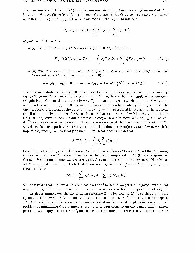
7.2. SECOND ORDER OPTIMALITY CONDITIONS 159
Proposition 7.2.1 Let � in (P �) be twice continuously di�erentiable in a neighbourhood of y� =0. If y� = 0 is locally optimal for (P �), then there exist uniquely de�ned Lagrange multipliers��i � 0, i = 1; :::; q, and ��j , j = 1; :::; k, such that for the Lagrange function
L�(y;�; �) = �(y) +qXi=1
��i�i(y) +kX
j=1
�q+j(y)
of problem (P �) one has:
� (i) The gradient in y of L� taken at the point (0;��; ��) vanishes:
ryL�(0;��; ��) � r�(0) +
qXi=1
��ir�i(0) +kX
j=1
��jr�k+j = 0 (7.2.1)
� (ii) The Hessian of L� in y taken at the point (0;��; ��) is positive semide�nite on thelinear subspace T � = fy j yk = ::: = yq+k = 0g:
d = (d1; :::; dn) 2 Rn; d1 = ::: = dq+k = 0) dTr2yL
�(0;��; ��)d � 0: (7.2.2)
Proof is immediate. (i) is the KKT condition (which in our case is necessary for optimalitydue to Theorem 7.1.2, since the constraints of (P �) clearly satis�es the regularity assumption(Regularity). We can also see directly why (i) is true: a direction d with di � 0;, i = 1; :::; q,and di = 0, i = q + 1; :::; q + k (the remaining entries in d can be arbitrary) clearly is a feasibledirection for our problem at the point y� = 0, i.e., y�+ td = td is feasible solution to the problemfor all small positive { in fact, for all positive { values of t. Since y� = 0 is locally optimal for(P �), the objective � locally cannot decrease along such a direction: dTr�(0) � 0. Indeed,if dTr�(0) were negative, then the values of the objective at the feasible solutions td to (P �)would be, for small positive t, strictly less than the value of the objective at y� = 0, which isimpossible, since y� = 0 is locally optimal. Now, what does it mean that
dTr�(x�) �nXi=1
di@
@yi�(0) � 0
for all d with the �rst q entries being nonpositive, the next k entries being zero and the remainingentries being arbitrary? It clearly means that the �rst q components of r�(0) are nonpositive,the next k components may me arbitrary, and the remaining components are zero. Now let usset ��i = � @
@yi�(0), i = 1; :::; q (note that ��i are nonnegative) and �
�j = � @
@yq+j�(0), j = 1; :::; k;
then the vector
r�(0) +qXi=1
��ir�i(0) +kX
j=1
��jr�q+j(0)
will be 0 (note that r�i are simply the basic orths of Rn), and we get the Lagrange multipliersrequired in (i); their uniqueness is an immediate consequence of linear independence of r�i(0).
(ii) also is immediate: the entire linear subspace T � is feasible for (P �), so that from localoptimality of y� = 0 for (P ) it follows that 0 is local minimizer of � on the linear subspaceT �. But we know what is necessary optimality condition for this latter phenomenon, since theproblem of minimizing � on a linear subspace is in equivalent to unconstrained minimizationproblem: we simply should treat T �, and not Rn, as our universe. From the above second order

160 LECTURE 7. OPTIMALITY CONDITIONS
necessary optimality condition for unconstrained minimization we conclude that the secondorder derivative of � taken at the point y� = 0 along any direction d 2 T �, i.e., the quantitydTr2�(0)d, should be nonnegative. But this quantity is the same as dTr2
yL�(0;��; ��)d, since
�(y) di�ers from L�(y;��; ��) by a linear function of y, and we come to (ii).
One may ask: why should we express a simple thing { nonnegativity of the second order
derivative of � taken at y� = 0 along a direction from T � { in that strange way { as similar
property of the Lagrange function. The answer is that this is the L�-form of this fact, not
the �-form of it, which is stable with respect to nonlinear substitutions of the argument and
is therefore appropriate for extension from the case of special problem (P �) to the case of
general optimization problem (P ).
Now we know what is the necessary second order optimality condition for our special problem(P �), and what we are about to do is to understand how the condition should be strengthened inorder to become suÆcient for local optimality. The second order part of our necessary conditionin fact comes from the second order part of the necessary optimality condition for the uncon-strained case { we simply replace the entire Rn by the \unconstrained part of the feasible set" {the linear subspace T �, and the condition says that r2�(0) � r2
yL�(0;��; ��) should be positive
semide�nite along the directions from T �. By analogy with the unconstrained case we couldguess that to make our necessary condition suÆcient, we should replace \positive semide�nite"in the latter sentence by \positive de�nite". The truth, however, is more sophisticated, as isseen from the following example:
�(y) = y22 � y21 ! min j �1(y) � y1 � 0
(q = 1, k = 0). Here the \�rst-order" part of the optimality condition from Proposition 7.2.1 issatis�ed with ��1 = 0, the linear subspace T � is T � = fd = (d1; d2) j d1 = 0g and the Hessian
of � taken at 0 and restricted to T � is positive de�nite: @2
@y22�(0) = 2 > 0. Nevertheless, y� = 0
clearly is not locally optimal, and we see that \naive" modi�cation of the condition { \replacedTr2L�d � 0 by dTr2L�d > 0 for nonzero d 2 T �" { does not work: it does not make thecondition suÆcient for local optimality.
The actual suÆcient condition for local optimality is as follows:
Proposition 7.2.2 Consider special optimization program (P �), and assume that the data �; �iare twice continuously di�erentiable in a neighbourhood of y� = 0. Assume also that there existLagrange multipliers ��i � 0, i = 1; :::; q, and ��j , j = 1; :::; k, such that for the Lagrange function
L�(y;�; �) = �(y) +qXi=1
�i�i(y) +kX
j=1
�j�q+j(y)
one has
� [�rst-order part] ryL�(0;��; ��) = 0
and
� [second-order part] dTr2yL
�(0;��; ��)d > 0 for all nonzero d from the linear subspace
T �� = fd 2 Rn j ��i di = 0; i = 1; :::; q; dq+1 = ::: = dq+k = 0g:
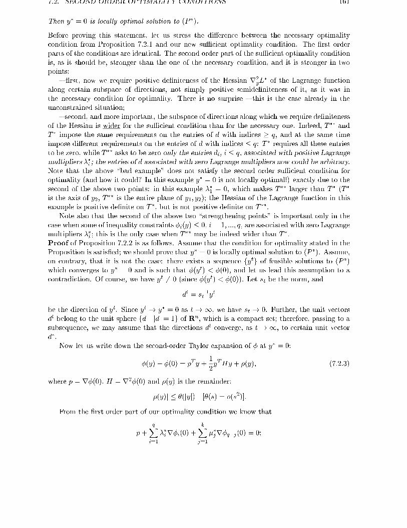
7.2. SECOND ORDER OPTIMALITY CONDITIONS 161
Then y� = 0 is locally optimal solution to (P �).
Before proving this statement, let us stress the di�erence between the necessary optimalitycondition from Proposition 7.2.1 and our new suÆcient optimality condition. The �rst orderparts of the conditions are identical. The second order part of the suÆcient optimality conditionis, as it should be, stronger than the one of the necessary condition, and it is stronger in twopoints:
{ �rst, now we require positive de�niteness of the Hessian r2yL
� of the Lagrange functionalong certain subspace of directions, not simply positive semide�niteness of it, as it was inthe necessary condition for optimality. There is no surprise { this is the case already in theunconstrained situation;
{ second, and more important, the subspace of directions along which we require de�nitenessof the Hessian is wider for the suÆcient condition than for the necessary one. Indeed, T �� andT � impose the same requirements on the entries of d with indices � q, and at the same timeimpose di�erent requirements on the entries of d with indices � q: T � requires all these entriesto be zero, while T �� asks to be zero only the entries di, i � q, associated with positive Lagrangemultipliers ��i ; the entries of d associated with zero Lagrange multipliers now could be arbitrary.Note that the above \bad example" does not satisfy the second order suÆcient condition foroptimality (and how it could? In this example y� = 0 is not locally optimal!) exactly due to thesecond of the above two points: in this example ��1 = 0, which makes T �� larger than T � (T �
is the axis of y2, T �� is the entire plane of y1; y2); the Hessian of the Lagrange function in thisexample is positive de�nite on T �, but is not positive de�nite on T ��.
Note also that the second of the above two \strengthening points" is important only in thecase when some of inequality constraints �i(y) � 0, i = 1; :::; q, are associated with zero Lagrangemultipliers ��i ; this is the only case when T �� may be indeed wider than T �.Proof of Proposition 7.2.2 is as follows. Assume that the condition for optimality stated in theProposition is satis�ed; we should prove that y� = 0 is locally optimal solution to (P �). Assume,on contrary, that it is not the case: there exists a sequence fytg of feasible solutions to (P �)which converges to y� = 0 and is such that �(yt) < �(0), and let us lead this assumption to acontradiction. Of course, we have yt 6= 0 (since �(yt) < �(0)). Let st be the norm, and
dt = s�1t yt
be the direction of yt. Since yt ! y� = 0 as t! 1, we have st ! 0. Further, the unit vectorsdt belong to the unit sphere fd j jdj = 1g of Rn, which is a compact set; therefore, passing to asubsequence, we may assume that the directions dt converge, as t ! 1, to certain unit vectord�.
Now let us write down the second-order Taylor expansion of � at y� = 0:
�(y)� �(0) = pT y +1
2yTHy + �(y); (7.2.3)
where p = r�(0), H = r2�(0) and �(y) is the remainder:
j�(y)j � �(jyj) [�(s) = o(s2)]:
From the �rst order part of our optimality condition we know that
p+qXi=1
��ir�i(0) +kX
j=1
��jr�q+j(0) = 0;

162 LECTURE 7. OPTIMALITY CONDITIONS
recalling what are �i, we conclude that (7.2.3) can be rewritten as
�(y)� �(0) = �qXi=1
��i yi �kX
j=1
��jyq+j +1
2yTHy + �(y): (7.2.4)
Substituting y = yt = stdT and taking into account that the entries with indices q + 1; :::; q + kin dt vanish (since yt is feasible for (P �)), we get
0 > s�1t [�(yt)� �(0)] =
"�
qXi=1
��i dti
#1
+ st
�1
2(dt)THdt + s�2t �(std
t)�2: (7.2.5)
Now let us make several simple observations:
� (a): The quantities [�]1 in the right hand side of (7.2.5) are nonnegative (since yt is feasible,we have dti � 0, i = 1; :::; q, while ��i are nonnegative);
� (b): As t!1, the quantities [�]1 converge to �Pqi=1 �
�i d�i � 0;
� (c): As t ! 1, the quantities [�]2 converge to 12(d
�)THd� (since j�(stdt)j � �(st) and�(s) = o(s2)), whence the quantities st[�]2 converge to 0.
Our �rst conclusion from these observations is that the right hand side of (7.2.5) converges, ast!1, to �Pq
i=1 ��i d�i � 0, while the left hand side is nonpositive, whence the limit of the right
hand side actually is equal to 0:
(!)qXi=1
��i d�i = 0:
Since the vector d� inherits from the vectors dt the property to have the �rst q coordinatesnonpositive and the next k coordinates zero, we see that every term ��i d
�i in the sum (!) is
nonpositive; since the sun is equal to 0, we conclude that ��i d�i = 0, i = 1; :::; q. Since, besides
this, d�q+j = 0; j = 1; :::; k, we conclude that d 2 T ��.Now let us divide both sides of (7.2.5) by st; taking into account observation (a), we shall
get the inequality0 � s�2t (�(yt)� �(0)) � [�]2:
From (c), the right hand side in this inequality converges, as t ! 1, to 12 (d
�)THd�, so thatthis quantity should be nonpositive. At the same time, we already know that d� 2 T �� and wefrom the very beginning know that jd�j = 1; thus, part (ii) of the optimality condition impliesthat 1
2(d�)THd� > 0 (note that r2�(0) = r2
yL�(0;��; ��): �i are linear!); this is the desired
contradiction.
From special case to the general one. Now we are in a position where we can easily achievethe second of our targets { to get the second order optimality conditions for the case of a generaloptimization problem (P ).
Theorem 7.2.1 [Second Order Optimality Conditions in Mathematical Programming]Consider constrained optimization program (P ), and assume that x� is a feasible solution to thisproblem, and the data f; g1; :::; gm; h1; :::; hk are twice continuously di�erentiable in a neighbour-hood of x�. Let also the regularity assumption (Regularity) be satis�ed: the taken at x� gradients

7.2. SECOND ORDER OPTIMALITY CONDITIONS 163
of active at the point constraints of (P ) are linearly independent. Finally, let
L(x;�; �) = f(x) +mXi=1
�igi(x) +kX
j=1
�jhj(x)
be the Lagrange function of the problem.(i) [Second Order Necessary Optimality Condition] If x� is locally optimal for (P ), then there
exist and are uniquely de�ned Lagrange multipliers ��i � 0 and ��j such that
� (��; ��) certify that x� is a KKT point of (P ):
��i gi(x�) = 0; i = 1; :::;m;
rxL(x�;��; ��) � rf(x�) +Pmi=1 �
�irgi(x�) +
Pkj=1 �
�jrhj(x�) = 0
(7.2.6)
� The Hessian r2xL(x
�;��; ��) of the Lagrange function in x is positive semide�nite on theorthogonal complement M� to the set of gradients of active at x� constraints:
d 2M� � fd j dTrgi(x�) = 0; i 2 I(x�); dTrhj(x�) = 0; j = 1; :::; kg )dTr2
xL(x�;��; ��)d � 0
(here I(x�) is the set of indices of active at x� inequality constraints).
(ii) [Second Order SuÆcient Optimality Condition] Assume that there exist Lagrange multi-pliers ��i � 0, ��j such that
� ��; �� certify that x� is a KKT point of (P ), i.e., (7.2.6) is satis�ed
� The Hessian r2xL(x
�;��; ��) of the Lagrange function in x is positive de�nite on the or-thogonal complement M�� to the set of gradients of equality constraints and those activeat x� inequality constraints which are associated with positive Lagrange multipliers ��i :
d 2M�� � fd j dTrgi(x�) = 0; i 2 J(x�); dTrhj(x�) = 0; j = 1; :::; kg; d 6= 0)dTr2
xL(x�;��; ��)d > 0
(here J(x�) is the set of indices of active at x� inequality constraints associated with positiveLagrange multipliers ��i ).
Then x� is locally optimal for (P ).
Proof. Without loss of generality, we may assume that the inequality constraints active at x�
are the �rst q inequality constraints. Now let us consider the q+ k functions g1; :::; gq ; h1; :::; hk;all these functions are equal to 0 at x�, and their gradients at the point are linearly indepen-dent. According to Theorem 7.1.1, there exists at least twice continuously di�erentiable in aneighbourhood Y of the point y� = 0 substitution of argument y 7! S(y), S(0) = x�, whichis a one-to-one mapping of Y onto a neighbourhood X of x�, has at least twice continuouslydi�erentiable in X inverse S�1(x) and \linearizes" the functions g1; :::; gq ; h1; :::; hk :
�i(y) � gi(S(y)) � yi; i = 1; :::; q;�i(y) � hi�q(S(y)) � yi; i = q + 1; :::; q + k:
Now let�(y) = f(S(y))

164 LECTURE 7. OPTIMALITY CONDITIONS
and consider the special problem
(P �) �(y)! min j �i(y) � 0; i = 1; :::; q; �i(y) = 0; i = q + 1; :::; q + k:
It is immediately seen that
� (a) the functions �; �i; i = 1; :::; q+k; are twice continuously di�erentiable in a neighbour-hood of y� = 0
� (b) x� is locally optimal solution for (P ) if and only if y� = 0 is locally optimal solutionfor (P �).
In view of these observations, we can get necessary/suÆcient conditions for local optimality ofx� in (P ) as direct \translations" of the already known to us optimality conditions for y� in(P �). The only thing we should understand what are the entities mentioned in (P �)-optimalityconditions in the \(P )-language". This is easy.
First of all, we can write
f(x) = �(R(x)); gi(x) = �(R(x)); i = 1; :::; q; hj(x) = �q+j(R(x)); j = 1; :::; k; (7.2.7)
where R(�) is S�1(�).Second, we have
S(R(x)) � x
in a neighbourhood of x�; di�erentiating this identity, we get
S0(0)R0(x�) = I
(I is the unit matrix), so that the matrix
Q = R0(x�)
is nonsingular.Third, we can forget about inequality constraints of (P ) which are non-active at x� { these
constraints neither in uence the property of x� to be locally optimal for (P ), nor participate inthe optimality conditions we are going to prove. The latter point should be explained: formally,non-active constraints do participate in the optimality conditions { they appear in the Lagrangefunction of (P ). But this is nothing but illusion (caused by our desire to write the conditionswith
Pmi=1 instead of
Pi2I(x�)): both the necessary and the suÆcient conditions in question
include complementary slackness ��i gi(x�) = 0, i = 1; :::;m, which implies that the Lagrange
multipliers associated with non-active gi are zeros; looking at our optimality conditions, weconclude that in fact the nonactive constraints do not enter them.
After we drop the non-active constraints (we just have seen that it can be done), the Lagrangefunctions of (P ) and (P �) become linked with each other by the same relation as the datafunctions of the problems:
L(x;�; �) = L�(R(x);�; �): (7.2.8)
Fourth, and the most important, from (7.2.8) and the rules of di�erentiating superpositionswe have the following relations:
rxL(x�;�; �) = QTryL
�(y�;�; �) (7.2.9)

7.2. SECOND ORDER OPTIMALITY CONDITIONS 165
and
vTr2xL(x
�;�; �)v = (Qv)Tr2yL
�(y�;�; �)(Qv) + [ryL�(0;�; �)]TR00[v];
where v is an arbitrary vector and
R00[v] =d2
dt2jt=0 R(x
� + tv)
is the second-order derivative of the mapping R(�) taken at x� along the direction v. It followsthat if � and � are such that ryL�(0;�; �) = 0, then the Hessians of L and L� in the primalvariables are linked by the simple relation
r2xL(x
�;�; �) = QTr2yL
�(0;�; �)Q (7.2.10)
which does not involve the \curvature" R00[�] of the substitution x 7! R(x) which converts (P )into (P �).
Since in the optimality conditions for (P �) we are speaking about the Lagrange multipliersfor (P �) make rL�(0;�; �) equal to zero, the latter observation makes the \translation" ofoptimality conditions from the (P �)-language to the (P )-language indeed easy. Let me showhow this translation is carried out for the necessary optimality condition; with this example, thereader de�nitely would be able to translate the suÆcient optimality condition by himself.
Thus, let us prove (i). Assume that x� is locally optimal for (P ). Then, according to theabove remarks, y� = 0 is locally optimal for (P �). By Proposition 7.2.1 the latter means thatthere exist ��i � 0 and ��j such that
(#) ryL�(0;��; ��) = 0(&) dTr2
yL�(0;��; ��)d � 0 8d 2 T � � fd j di = 0; i = 1; :::; q + kg :
Let us verify that the above �� and �� are exactly the entities required in (i)2). First, we shouldnot bother about complementary slackness ��i gi(x
�) = 0 { see the \recall" in the latter footnote.Second, we do have the Euler equation rxL(x�;��; ��) = 0, since we have similar equation (#)for L� and we have the chain rule (7.2.9). Thus, we do have the �rst-order part of (i). To getthe second-order part, note that we have similar statement (&) for L�, and from (#) it followsthat we have also the \chain rule" (7.2.10), so that we have the inequality
dTr2xL(x
�;��; ��)d � 0 8d : Qd 2 T �: (7.2.11)
It remains to understand what does it mean thatQd 2 T �. We have �i(y) � yi, gi(x) = �i(R(x)),i = 1; :::; q, and hj(x) = �q+j(R(x)), which, in simple words, means that the vector-functioncomprised of g1; :::; gq ; h1; :::; hk is nothing but the (q + k)-dimensional initial fragment of then-dimensional vector-function R. Since Q = R0(x�), the �rst q + k entries of the vector Qd areexactly the inner products of the taken at x� gradients of g1; :::; gq ; h1; :::; hk with the directiond; to say that Qd 2 T � is the same as to say that all these inner products are zero (recall thatT � is the subspace of vectors with �rst q+ k entries equal to 0), i.e., to say that d 2M�. Thus,(7.2.11) is exactly the second-order part of (i).
2)recall that we have reduced the situation to the case when all inequality constraints in (P ) are active atx�; otherwise I would be supposed to say: \Let us take ��i 's coming from (P �) as the required in (i) Lagrangemultipliers for the active inequality constraints, and let us set the Lagrange multipliers of nonactive constraintsto zeros"

166 LECTURE 7. OPTIMALITY CONDITIONS
Remark 7.2.1 Now we understand what for we formulated the second-order parts ofthe optimality conditions in Propositions 7.2.1, 7.2.2 in terms of the Hessian of the Lagrangefunction and not the objective (although in the case of special problem (P �) the Hessian ofthe Lagrangian is exactly the same as the Hessian of the objective). Only the formulation interms of the Lagrange function remains invariant under nonlinear substitutions of argument{ the tool we used to get the optimality conditions in the general case as an immediateconsequences of the same conditions for the simple special case.
Geometry of Second Order Optimality Conditions. In fact Second Order Op-timality Conditions say to us very simple things. To see it, we �rst should understand thegeometry of the linear subspace M� involved into the necessary condition. This is the sub-space we get as follows: we take all constraints of the problem which are active at locallyoptimal solution x�, linearize them at this point and take the aÆne set which is given bythe system of linear equations \linearizations of the active constraints are equal to 0"; thisaÆne set is exactly x�+M�. What is this set geometrically? Nothing but the tangent planeto the surface S where all constraints active at x� still are active. Thus, directions from M�
are the directions tangent to S at x�. If S is enough regular (as it is under the regularityassumption), moving from x� \forward" and \backward" along such a direction, we stay\very close" to S { the distance from S is in�nitesimal of highest order as compared to thestep along the direction. It follows that if x� is locally optimal, then no tangent directioncould be direction of decrease of the objective. Indeed, otherwise we could improve x� by(1) performing a small step along this tangent direction (it would improve the objective bysomething which is of the same order of magnitude as the step). Of course, this displacement,generally speaking, pushes us out of the feasible set, but we still are very close to it { thedistance to the feasible set cannot be larger than the distance to S, and the latter distance ismuch smaller than the step we did. It follows that if we accompany (1) by \correction" (2){ movement from the point given by (1) to the closest feasible point { we perhaps loose inthe value of the objective, but the losses are very small { of the highest order as comparedto the length of the step (1). The balance, for small stepsizes, would be in our favour {in (1), we gain something almost proportional to the stepsize, in (2) loose something whichis much smaller than the stepsize. But a locally optimal solution cannot be improved bysmall modi�cation, and we conclude that there exist no input to our mechanism { no tangentdirection which is a direction of decrease for the objective. In other words,
the gradient of the objective at a locally optimal solution x� should be orthogonal to the(tangent plane of the) surface S of active constraints.
This is partial \geometrical translation" of the �rst order part of the KKT condition. Indeed,we know what is the tangent plane in question { it is the orthogonal complement to the setof gradients of active constraints; the standard Linear Algebra fact (X?)? = Lin(X) meansthat it is the same { to say that certain vector is orthogonal to tangent plane and to saythat the vector is a linear combination of the gradients of active constraints, as it is saidin the KKT condition. Note that in the case of equality constrained problem the KKTcondition says nothing else, so that in this case orthogonality of rf(x�) and S is complete,not partial, geometrical interpretation of the condition. In the inequality constrained case,the KKT condition provides us with additional information: it says what should be thesigns of coeÆcients at the gradients of inequality constraints in the representation of rf(x�)(these coeÆcients should be � 0). This conclusion comes from the fact that at a locallyoptimal x� the objective has no right to decrease not only along direction tangent to S, butalso along those tangent to the surface given by equality constraints and leading inside the\curved half-spaces" given by active inequality constraints. We see that the KKT condition{ the �rst-order part of the second order necessary optimality condition { is very geometric.
What about the geometry of the second-order part of the condition? A naive guess wouldbe like this:

7.3. CONCLUDING REMARKS 167
\if x� is locally optimal, we for sure are unable to improve the objective bysmall displacements along S. Perhaps it mean that we are unable to improve theobjective by small displacements along the tangent to S plane x� +M� as well{ this tangent plane locally is so close to S! If our guess is true, it means thatx� is local minimizer of the objective on the tangent plane, and we know whatdoes it mean { the gradient of the objective at x� should be orthogonal to M�,and the second order derivative of it along every direction from M� should benonnegative".
The above reasoning is absolutely false. The second order part of the \unconstrained" opti-mality condition { \the second order derivative along any direction should be nonnegative"{ comes from analyzing second-order e�ects caused by small perturbations of x�, and thetangent plane does not, normally, approximate a curved surface within second-order terms.It follows that the second-order phenomena we met when traveling along a curved surfaceare not the same as those when traveling along the tangent plane to this surface, so that theconclusions derived from analyzing these \plane" phenomena may have nothing in commonwith reality. For example, in the optimization problem
�0:01x21 ! min j x21 + x22 = 1
the point x� = (0; 1) clearly is locally optimal, in spite of the fact that the second orderderivative of the objective taken at x� along the tangent line fx2 = 1g to the feasiblecircumference is negative.
It turns out that this is the second order derivative of the Lagrange function (with prop-
erly chosen Lagrange multipliers), not the one of the objective, which should be nonnegative
along tangent directions to S at a local optimum, and this is the main moral which can be
extracted from the second order optimality conditions.
7.3 Concluding Remarks
It was announced in the preface to the course and to this lecture that optimality conditions insome cases allow to �nd closed form solutions to optimization problems. After we know whatare the optimality conditions, it is time to explain how one can use them to solve a problem \onthe paper". The scheme is very simple. Given a constrained optimization problem (P ), we canwrite down the KKT optimality conditions along with the feasibility requirements:
rf(x�) +Pmi=1 �
�irgi(x�) +
Pkj=1 �
�jrhj(x�) = 0 [n = dim x equations]��i gi(x
�) = 0; i = 1; :::; :m [m equations]hj(x�) = 0; j = 1; :::; k [k equations]gi(x�) � 0; i = 1; :::;m
��i � 0; i = 1; :::;m
The equality part of this system is a system of n+m + k nonlinear equations with n+m+ kunknowns { the entries of x�; ��; ��. Normally such a system has only �nitely many solutions. Ifwe are clever enough to �nd all these solutions and if by some reason we know that the optimalsolution exists and indeed satis�es the KKT condition (e.g., the assumptions of Theorem 7.1.2are satis�ed at every feasible solution), then we may be sure that looking through all solutions tothe KKT system and choosing among them the one which is feasible and has the best value of theobjective, we may be sure that we shall end up with the optimal solution to the problem. In thisprocess, we may use the inequality part of the system (same as the additional inequalities comingfrom the second order necessary optimality conditions) to eliminate from the list candidates

168 LECTURE 7. OPTIMALITY CONDITIONS
which do not satisfy the inequalities, which enables to skip more detailed analysis of thesecandidates.
Approach of this type is especially fruitful if (P ) is convex (i.e., f; g1; :::; gm are convexand h1; :::; hk are linear). The reason is that in this case the KKT conditions are suÆcientfor global optimality (we know it from the previous Lecture, although for the case when thereare no equality constraints; the extension to the case of linear equality constraints is quitestraightforward). Thus, if the problem is convex and we are able to point out a single solutionto the KKT system, then we can be sure that it is the actual { globally optimal { solution to(P ), and we should not bother to look for other KKT points and compare then with each other.
Unfortunately, the outlined program can be carried out in simple cases only; normally non-linear KKT system is too diÆcult for analytical solution. Let us look at one { and a veryinstructive one { of \simple cases".
Minimizing a homogeneous quadratic form over the unit sphere. Consider the prob-lem
(Q) f(x) � xTAx! min j g1(x) � xTx� 1 � 0;
A being a symmetric n� n matrix. Let us list all locally optimal solutions to the problem.Step 0. Let f� denote the optimal value. Since x = 0 clearly is feasible solution and
f(0) = 0, we have f� � 0. There are, consequently, two possible cases:Case (A): f� = 0;Case (B): f� < 0.Step 1: Case (A). Case (A) takes place if and only if xTAx � 0 for all x, jxj � 1, or,
which is the same due to homogeneity with respect to x, if and only if
xTAx � 0 8x:
We know that symmetric matrices with this property have special name { they are called sym-metric positive semide�nite (we met with these matrices in this Lecture and also in the Convexitycriterion for twice continuously di�erentiable functions: such a function is convex in certain openconvex domain if and only if the Hessian of the function at any point of the domain is positivesemide�nite). In Linear Algebra there are tests for positive semide�niteness (the Sylvester rule:a symmetric matrix is positive semide�nite if and only if all its principal minors { those formedby several rows and the columns with the same indices as rows { are nonnegative). Now, whatare the locally optimal solutions to the problem in the case of positive semide�nite A? I claimthat these are exactly the points x from the unit ball (the feasible set of the problem) whichbelong to the kernel of A, i.e., are such that
Ax = 0:
First of all, if x possesses the latter property, then xTAx = 0 = f�, so that x� is even globallyoptimal. Vice versa, assume that x is locally optimal, and let us prove that Ax = 0. Theconstraint in our problem is convex; the objective also is convex (recall the criterion of convexityfor smooth functions and note that f 00(x) = 2A), so that a locally optimal solution is in factoptimal. Thus, x is locally optimal if and only if xTAx = 0. In particular, if x is locally optimal,then, say, x0 = x=2 also is. At this new locally optimal solution, the constraint is satis�ed asa strict inequality, so that x0 is an unconstrained local minimizer of function f(�), and by theFermat rule we get rf(x0) � 2Ax0 = 0, whence also Ax = 0, as claimed.

7.3. CONCLUDING REMARKS 169
Step 2: Case (B). Now consider the case of f� < 0, i.e., the one when there exists h,jhj � 1, such that
(#) hTAh < 0:
What are the locally optimal solutions x� to the problem?
What is said by the First Order Optimality conditions. Logically, two possibilities can takeplace: the �rst is that jx�j < 1, and the second is that jx�j = 1.
Let us prove that the �rst possibility if in fact impossible. Indeed, in the case of jx�j <1 x� should be locally optimal in the unconstrained problem f(x) ! min j x 2 Rn withsmooth objective. By the second order necessary condition for unconstrained local optimality,the Hessian of f at x� (which is equal to 2A) should be positive semide�nite, which contradicts(#).
Thus, in the case in question a locally optimal solution x� is on the boundary of the unitball, and the constraint g1(x) � 0 is active at x�. The gradient 2x� of this constraint is thereforenonzero at x�, so that (by Theorem 7.1.2) x� is a KKT point:
9��1 � 0 : rf(x�) + ��1rg1(x�) = 0;
or, which is the same,Ax� = ���1x�:
Thus, x� should be a unit eigenvector3 of A with a nonpositive eigenvalue � � ���1; this is allwhich we can extract from the First Order Necessary Optimality conditions.
Looking at the example
A = Diag(1; 0;�1;�2;�3; :::;�8)
in R10, we see that the First Order Necessary optimality conditions are satis�ed by 18 vectors�e2;�e3; :::;�e10, where e1, i = 1; :::; 10, are the standard basic orths inR10. All these 18 vectorsare Karush-Kuhn-Tucker points of the problem, and the First Order Optimality conditions donot allow to �nd out which of these 18 candidates are locally optimal and which are not. To getthe answer, we should use the Second Order Optimality conditions.
What is said by the Second Order Optimality conditions. We come back to our general problem(Q); recall that we are in the case of (B). We already know that a locally optimal solution to(Q) is a unit vector, and the set of constraints active at x� is comprised of our only inequalityconstraint; its gradient 2x� at x� is nonzero, so that we have (Regularity), and consequentlyhave the Second Order Necessary Optimality condition (Theorem 7.2.1.(i)). Thus, there shouldexist Lagrange multiplier ��1 � �� � 0 such that
2Ax� � 2�x� � rf(x�) + ��1rg1(x�) = 0
anddT [2A� 2�I]d � dT [r2f(x�) + ��1r2g1(x
�)]d � 0
(I is the unit matrix) for any d satisfying the condition
dTrg1(x�) � 2dTx� = 0:3recall that an eigenvector of a square matrix M is a nonzero vector e such that Me = sx for certain real s
(this real is called the eigenvalue of M associated with the eigenvector e.

170 LECTURE 7. OPTIMALITY CONDITIONS
In other words, at x� we should have, for certain � � 0,
Ax� = �x� (7.3.1)
anddT (A� �I)d � 0 (7.3.2)
for all d such thatdTx� = 0:
Let us prove that in fact (7.3.2) is valid for all d 2 Rn. Indeed, given a d 2 Rn, we candecompose it as
d = d1 + d2;
where d1 is the orthogonal projection of d onto the one-dimensional subspace spanned by x�,and d2 is the orthogonal projection of d onto the orthogonal complement to x�:
d1 = �x�; dT2 x� = 0:
We have
dT (A� �I)d = (d1 + d2)T (A� �I)(d1 + d2) = dT1 (A� �I)d1 + 2dT2 (A� �I)d1 + dT2 (A� �I)d2;
from d1 = �x1 and from (7.3.1) it follows that the �rst two terms { those containing d1 { in thelast expression are zero, and from (7.3.2) it follows that the third term is nonnegative (recallthat dT2 x
� = 0). Consequently, the expression is nonnegative, as claimed.We conclude that a locally optimal solution x� of the problem (Q) should be a unit vector
such that x� is an eigenvector of A with a nonpositive eigenvalue � and, besides this, such thatthe matrix A � �I should be positive semide�nite { (7.3.2) should be valid for all d. It followsthat � is the smallest of eigenvalues of A: indeed, if �0 is another eigenvalue, so that there existsa nonzero x0 with Ax0 = �0x0, then we should have
0 � (x0)T (A� �I)x0 � (x0)T (�0 � �)x0 = (�0 � �)jx0j2;whence �0 � �.
We conclude that the � - the minus Lagrange multiplier associated with a locally optimalsolution x� is uniquely de�ned by the problem: this is the smallest eigenvalue of A. And since
f(x�) = (x�)TAx� = �jx�j2 = �
(we already know that a locally optimal solution must be a unit eigenvector of A with theeigenvalue �), we conclude that the value of the objective at a locally optimal solution alsois uniquely de�ned by the problem. Since the problem clearly is solvable (the feasible set iscompact and the objective is continuous), locally optimal solutions exist and among them thereare optimal ones; and since the objective, as we have seen, is constant on the set of locallyoptimal solutions, we conclude that
In the case of (B) locally optimal solutions are the same as optimal ones and all of them areunit eigenvectors of A associated with the smallest eigenvalue of the matrix.
On the other hand, if x� is a unit eigenvector of A with the eigenvalue �, then f(x�) = � (see theabove computation), so that all unit eigenvectors of A associated with the smallest eigenvalueof the matrix are, in the case of (B), optimal solutions to (Q). We see that the Second OrderNecessary Optimality condition, in contrast to the First Order one, allows us to get completedescription of the solutions to (Q).

7.3. CONCLUDING REMARKS 171
Remark 7.3.1 A byproduct of our reasoning is the statement that if a symmetric matrix Asatis�es (#), then there exists an eigenvector of A ((Q) for sure is solvable, and the First OrderNecessary condition says, as we have seen, that an optimal solution must be an eigenvector).Note that it is far from being clear in advance why a symmetric matrix should have an eigenvec-tor. Of course, our reasoning establishes the existence of an eigenvector only under assumption(#), but this restriction can be immediately eliminated (given an a arbitrary symmetric matrixA0, one can apply the reasoning to the matrix A = A0 � TI which, for large T , for sure satis�es(#), and to get existence of an eigenvector of A; of course, it will be also an eigenvector of A0).
The existence of an eigenvector for a symmetric matrix is, of course, a perfectly well knownelementary fact of Linear Algebra; here is a several-line proof:
Let us prove �rst that an arbitrary matrix A, even with complex entries, possesses a complexeigenvalue. Indeed, � is an eigenvalue of A if and only if there exists a nonzero (complex)vector z such that (A��I)z = 0, i.e., if and only if the matrix �I�A is singular, or, which isthe same, the determinant of the matrix is zero. On the other hand, the determinant of thematrix �I �A clearly is a nonconstant polynomial of �, and such a polynomial, according toFTA { the Fundamental Theorem of Algebra { has a root; such a root is an eigenvalue of A.Now we should prove that if A is real and symmetric, then it has a real eigenvalue and areal eigenvector. This is immediate: we simply shall prove that all eigenvalues of A are real.Indeed, if � is an eigenvalue of A (regarded as a complex matrix) and z is the corresponding(complex) eigenvector, then the expression
nXi;j=1
Aijzjz�i
(� means complex conjugation) is real (look at its conjugate!); on the other hand, for the
eigenvector z we haveP
j Aijzj = �zi, so that our expression is �Pn
i=1 ziz�i = �
Pni=1 jzij2;
since z 6= 0, this latter expression can be real if and only if � is real.
Finally, after we know that an eigenvalue � of a real symmetric matrix (regarded as a matrix
with complex entries) in fact is real, we can immediately prove that the eigenvector associated
with this eigenvalue also can be chosen to be real: indeed, the real matrix �I �A is singular
and has therefore a nontrivial kernel.
In fact all results of our analysis of (Q) can be immediately derived from several other basic factsof Linear Algebra (namely, from possibility to represent a quadratic form xTAx in a diagonalform
Pni=1 �iu
2i (x), ui(x) being the coordinates of x in a properly chosen orthonormal basis).
Thus, in fact in our particular example the Optimization Theory with its Optimality conditionsis, in a sense, redundant. Two things, however, should be mentioned:
� The Linear Algebra proof of the existence of an eigenvector is based on the FTA whichstates existence of a (complex) root of a polynomial. To get the same result on theexistence of an eigenvector, in our proof (and in all the proofs it is based upon) we neverused something like FTA! All we used from Algebra was the elementary theory of systemsof linear equations, and we never thought about complex numbers, roots of polynomials,etc.!
This is an example of what is Mathematics, and it would be very useful exercise for amathematician to trace back both theories to see what are the \common roots" of twoquite di�erent ways to prove the same fact4).
4)the only solution to this exercise which comes to my mind is as follows: the simplest proof of the Fundamental

172 LECTURE 7. OPTIMALITY CONDITIONS
� It is worthy of mentioning that the Optimization Theory (which seems to be redundantto establish the existence of an eigenvector of a symmetric matrix) becomes unavoidablewhen proving a fundamental in�nite-dimensional generalization of this fact: the theorem(Hilbert) that a compact symmetric linear operator in a Hilbert space possesses an eigen-vector [and, �nally, even an orthonormal basis comprised of eigenvectors]. I am not goingto explain what all these words mean; roughly speaking, it is said that a in�nite dimen-sional symmetric matrix can be diagonalized in a properly chosen orthonormal basis (e.g.,an integral operator f(s) 7! R 1
0 K(t; s)f(s)ds with not that bad (e.g., square summable)symmetric (K(t; s) = K�(s; t)) kernel K possesses a complete in L2[0; 1] orthonormal sys-tem of eigenfunctions; this fact, in particular, explains why the atomic spectra are discreterather than continuous). When proving this extremely important theorem, one cannot useLinear Algebra tools (there are no determinants and polynomials anymore), but still canuse the optimization ones (compactness of the operator implies solvability of the corre-sponding problem (Q), and the �rst order necessary optimality condition which in the casein question says that the solution is an eigenvector of the operator, in contrast to FTA, is\dimension-invariant" and remain valid in the in�nite-dimensional case as well).
Theorem of Algebra is of optimization nature. This hardly is the complete answer, since the initial proof of FTAgiven by Gauss is not of optimization nature; the only fact from Analysis used in this proof is that a continuousfunction on the axis which takes both positive and negative values has a zero (Gauss used this fact for a polynomialof an odd degree). This is too far relationship, I think.
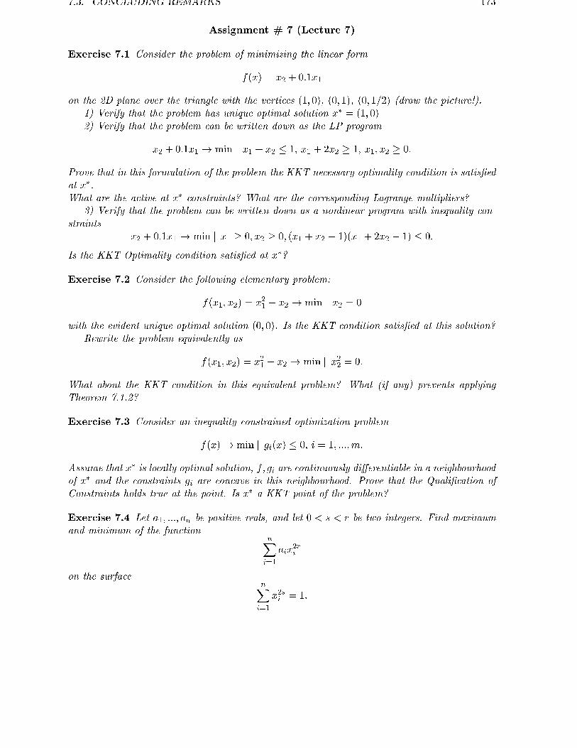
7.3. CONCLUDING REMARKS 173
Assignment # 7 (Lecture 7)
Exercise 7.1 Consider the problem of minimizing the linear form
f(x) = x2 + 0:1x1
on the 2D plane over the triangle with the vertices (1; 0), (0; 1), (0; 1=2) (draw the picture!).1) Verify that the problem has unique optimal solution x� = (1; 0)2) Verify that the problem can be written down as the LP program
x2 + 0:1x1 ! min j x1 + x2 � 1; x1 + 2x2 � 1; x1; x2 � 0:
Prove that in this formulation of the problem the KKT necessary optimality condition is satis�edat x�.What are the active at x� constraints? What are the corresponding Lagrange multipliers?
3) Verify that the problem can be written down as a nonlinear program with inequality con-straints
x2 + 0:1x1 ! min j x1 � 0; x2 � 0; (x1 + x2 � 1)(x1 + 2x2 � 1) � 0:
Is the KKT Optimality condition satis�ed at x�?
Exercise 7.2 Consider the following elementary problem:
f(x1; x2) = x21 � x2 ! min j x2 = 0
with the evident unique optimal solution (0; 0). Is the KKT condition satis�ed at this solution?Rewrite the problem equivalently as
f(x1; x2) = x21 � x2 ! min j x22 = 0:
What about the KKT condition in this equivalent problem? What (if any) prevents applyingTheorem 7.1.2?
Exercise 7.3 Consider an inequality constrained optimization problem
f(x)! min j gi(x) � 0; i = 1; :::;m:
Assume that x� is locally optimal solution, f; gi are continuously di�erentiable in a neighbourhoodof x� and the constraints gi are concave in this neighbourhood. Prove that the Quali�cation ofConstraints holds true at the point. Is x� a KKT point of the problem?
Exercise 7.4 Let a1; :::; an be positive reals, and let 0 < s < r be two integers. Find maximumand minimum of the function
nXi=1
aix2ri
on the surfacenXi=1
x2si = 1:

174 LECTURE 7. OPTIMALITY CONDITIONS

Lecture 8
Optimization Methods: Introduction
This lecture starts the second part of our course; what we are interested in from now on arenumerical methods for nonlinear continuous optimization, i.e., for solving problems of the type
minimize f(x) s.t. gi(x) � 0; i = 1; :::;m; hj(x) = 0; j = 1; :::; k: (8.0.1)
Here x varies overRn, and the objective f(x), same as the functions gi and hj , are smooth enough(normally we assume them to be at least once continuous di�erentiable). The constraints
gi(x) � 0; i = 1; :::;m; hj(x) = 0; j = 1; :::; k
are referred to as functional constraints, divided in the evident manner into inequality andequality constraints.
We refer to (8.0.1) as to nonlinear optimization problems in order to distinguish betweenthese problems and Linear Programming programs; the latter correspond to the case when allthe functions f; gi; hj are linear. And we mention continuous optimization in the description ofour subject to distinguish between it and discrete optimization, where we look for a solutionfrom a discrete set, e.g., comprised of vectors with integer coordinates (Integer Programming),vectors with 0-1 coordinates (Boolean Programming), etc.
Problems (8.0.1) arise in huge variety of applications, since whenever people make decisions,they try to make them in an \optimal" manner. If the situation is simple enough, so that thecandidate decisions can be parameterized by �nite-dimensional vectors, and the quality of thesedecisions can be characterized by �nite set of \computable" criteria, the concept of \optimal"decision typically takes the form of problem (8.0.1). Note that in real-world applications thispreliminary phase { modeling the actual decision problem as an optimization problem withcomputable objective and constraints { is, normally, much more diÆcult and creative than thesubsequent phase when we solve the resulting problem. In our course, anyhow, we do not touchthis modeling phase, and focus on technique for solving optimization programs.
Recall that we have developed optimality conditions for problems (8.0.1) in Lecture 7. Weremember that one can form a square system of nonlinear equations and a system of inequalitieswhich together de�ne certain set { the one of Karush-Kuhn-Tucker points of the problem {which, under mild regularity conditions, contains all optimal solutions to the problem. TheKarush-Kuhn-Tucker system of equations and inequalities typically has �nitely many solutions,and if we are clever enough to �nd all of them analytically, then we could look through themand to choose the one with the best value of the objective, thus getting the optimal solutionin a closed analytical form. The diÆculty, however, is that as a rule we are not so clever
175

176 LECTURE 8. OPTIMIZATION METHODS: INTRODUCTION
to solve analytically the Karush-Kuhn-Tucker system, same as are unable to �nd the optimalsolution analytically by other means. In all these \diÆcult" cases { and basically all optimizationproblems coming from real world applications are diÆcult in this sense { all we may hope for isa numerical routine, an algorithm which allows to approximate numerically the solutions we areinterested in. Thus, numerical optimization methods form the main tool for solving real-worldoptimization problems.
8.1 Preliminaries on Optimization Methods
It should be stressed that one hardly can hope to design a single optimization method capableto solve eÆciently all nonlinear optimization problems { these problems are too diverse. Infact there are numerous methods, and each of them is oriented onto certain restricted family ofoptimization problems.
8.1.1 Classi�cation of Nonlinear Optimization Problems and Methods
Traditionally, the Nonlinear Optimization Problems (8.0.1) are divided into two large classes:
� Unconstrained problems { no inequality or equality constraints are present. The genericform of an unconstrained problem, consequently, is
minimize f(x) s.t. x 2 Rn; (8.1.1)
f being smooth (at least once continuously di�erentiable) function on Rn;
� Constrained problems, involving at least one inequality or equality constraint.
The constrained problems, in turn, are subdivided into several classes, according to whetherthere are nonlinear constraints, inequality constraints, and so on; in the mean time we shallspeak about this in more details.
According to the outlined classi�cation of optimization problems, the optimization methodsare primarily partitioned into those for unconstrained and constrained optimization. Althoughthe more simpler unconstrained problems are not that frequently met in applications, meth-ods for unconstrained optimization play very important role: they are used directly to solveunconstrained problems and indirectly, as building blocks, in many methods of constrainedminimization.
8.1.2 Iterative nature of optimization methods
Methods for numerical solving nonlinear optimization problems are, in their essence, iterativeroutines: as applied to problem (8.0.1), a method typically is unable to �nd exact solutionin �nite number of computations. What a method generates, is an in�nite sequence fxtg ofapproximate solutions. The next iterate xt+1 is formed, according to certain rules, on thebasis of local information of the problem collected along the previous iterates. The portion ofinformation It obtained at a current iterate xt is a vector comprised of the values of the objectiveand the constraints at xt and, possibly, of the gradients or even higher-order derivatives of thesefunctions at xt. Thus, when forming xt+1, the method \knows" the values and the derivatives, upto certain �xed order, of the objective and the constraints at the previous iterates x1; :::; xt, andthis information is all information on the problem available to the method when it generates the
8.1. PRELIMINARIES ON OPTIMIZATION METHODS 177
new iterate xt+1. This iterate, consequently, is certain function of the information accumulatedso far:
xt+1 = Xt+1(I1;I2; :::;It):The collection of the search rules Xt(�) predetermines behaviour of the method as applied to anarbitrary problem; consequently, the method itself can be identi�ed with the collection fXtg1t=1.Note that the list of arguments in Xt is comprised of (t � 1) portions of local information; inparticular, the list of arguments in the very �rst search rule X1 is empty, so that this \function"is simply a �xed vector speci�ed by the description of the method { the starting point.
From the outlined general scheme of an iterative routine it follows that optimization methodsare classi�ed not only according to the types of problems the methods are solving, but alsoaccording to the type of local information they use. From this \information" viewpoint, themethods are divided into
� zero-order routines using only values of the objective and the constraints and not usingtheir derivatives;
� �rst-order routines using the values and the gradients of the objective and the constraints;
� second-order routines using the values, the gradients and the Hessians (i.e., matrices ofsecond-order derivatives) of the objective and the constraints.
In principle, of course, we could speak about methods of orders higher than 2; these methods,however, are never used in practice. Indeed, to use a method of an order k, you should providepossibility to compute partial derivatives of the objective and the constraints up to order k. Inthe multi-dimensional case it is not that easy even for k = 1 and even in the case when yourfunctions are given by explicit analytical expressions (which is not always the case). And thereis \explosion of diÆculties" in computing higher order derivatives: for a function of n variables,there are n �rst order derivatives to be computed, n(n+1)
2 second order derivatives, n(n+1)(n+2)2�3
third order derivatives, etc.; as a result, even in the medium-scale case with n being several tensthe diÆculties with programming, computation time, memory required to deal with higher-orderderivatives make exploiting these derivatives too expensive. On the other hand, there are noserious theoretical advantages in methods of order higher than 2, so there is no compensationfor the e�ort of computing these derivatives.
8.1.3 Convergence of Optimization Methods
As a matter of fact, we cannot expect a nonlinear problem to be solved exactly in �nite numberof steps; all we can hope for is that the sequence of iterates fxtg generated by the method inquestion converges, as t ! 1, to the solution set of the problem. In the theory of NumericalOptimization, the convergence of an optimization method on certain family of problems is exactlywhat gives the method right to be quali�ed as a tool for solving problems from the family.Convergence is not the only characteristic of a method, but this is the property which makes amethod theoretically valid optimization routine.
Rates of convergence
The fact of convergence of an optimization (and any other) computational method is the \weak-est" property which gives the method right to exist. In principle, there are as many methodswith this property as you wish, and the question is how to rank these methods and which of

178 LECTURE 8. OPTIMIZATION METHODS: INTRODUCTION
them to recommend for practical usage. In the traditional Nonlinear Optimization this problemis resolved by looking at the asymptotic rate of convergence measured as follows.
Assume that the method as applied to problem P generates sequence of iteratesconverging to the solution set X�
P of the problem. To de�ne the rate of convergence,we �rst introduce an error function err(x) which measures the quality of an approx-imate solution x; this function should be positive outside X�
P and should be zero atthe latter set.
There are several reasonable choices of the error function. E.g., we always canuse as it the distance from the approximate solution to the solution set:
distP (x) = infx�2X�P
jx� x�j;
another choice of the error function could be the residual in terms of the objectiveand constraints, like
resP (x) = maxff(x)� f�; [g1(x)]+; :::; [gm(x)]+; jh1(x)j; :::; jhk(x)jg;
f� being the optimal value in P and [a]+ = max(a; 0) being the positive part of areal a, etc.
For properly chosen error function (e.g., for distP ), convergence of the iterates tothe solution set implies that the scalar sequence
rt = err(xt)
converges to 0, and we measure the quality of convergence by the rate at which thenonnegative reals rt tend to zero.
The standard classi�cation here is as follows:
� [linear convergence] a sequence frt � 0g such that for some q 2 (0; 1), some C < 1 andall t one has
rt � Cqt
is called linearly converging to 0 with ratio q; the simplest example of such a sequenceis rt = Cqt. The lower bound of those q for which frtg linearly converges to 0 with theconvergence ratio q is called the convergence ratio of the sequence.
E.g., for the sequence rt = Cqt, same as for the sequence frt = C(q+�t)tg, �t ! 0; t!1,the convergence ratio is q, although the second sequence, generally speaking, does notconverge to 0 with the ratio q (it, anyhow, converges to 0 linearly with convergence ratioq0 for any q0 2 (q; 1)).
It is immediately seen that a suÆcient condition for a sequence frt > 0g to be linearlyconverging with ratio q 2 (0; 1) is to satisfy the property
lim supt!1rt+1
rt< q:
� [sub- and superlinear convergence] a sequence which converges to 0, but is not linearlyconverging (e.g., the sequence rt = t�1), is called sublinearly converging. A sequence

8.1. PRELIMINARIES ON OPTIMIZATION METHODS 179
which linearly converges to zero with any positive ratio (so that the convergence ratio ofthe sequence is 0) is called superlinearly converging (e.g., the sequence rt = t�t).
A suÆcient condition for a sequence frt > 0g to be superlinearly converging islimt!1
rt+1
rt= 0:
� [convergence of order p > 1] a sequence frt � 0g converging to 0 is called to have conver-gence order p > 1, if for some C and all large enough t one has
rt+1 � Crpt :
The upper bound of those p for which the sequence converges to 0 with order p is calledthe order of convergence of the sequence.
E.g., the sequence rt = a(pt) (a 2 (0; 1); p > 1) converges to zero with order p, since
rt+1=rpt = 1. The sequences converging to 0 with order 2 have special name { they are
called quadratically convergent.
Of course, a sequence converging to 0 with order p > 1 is superlinearly converging to 0(but, generally speaking, not vice versa).
Traditionally, the rate of convergence of iterative numerical routines is measured by the rankof the corresponding sequence of errors frt = err(xt)g in the above scale; in particular, wemay speak about sublinearly, linearly, superlinearly, quadratically converging methods, sameas about methods with order of convergence p > 1. It is common to think that the betteris the rate of convergence of a method, the more preferable is the method itself. Thus, alinearly converging method is thought to be better than a sublinearly converging one; amongtwo linearly converging methods the more preferable is the one with the smaller convergenceratio; a superlinearly converging method is preferred to a linearly converging one, etc. Ofcourse, all these preferences are \conditional", provided that there are no signi�cant di�erencesin computational complexity of steps, etc.
We should stress that the rate of convergence, same as the very property of convergence, isan asymptotic characteristic of the sequence of errors; it does not say when the announced rateof convergence occurs, i.e., what are the values of C or/and \large enough" values of t mentionedin the corresponding de�nitions. For concrete methods, the bounds on the indicated quantitiestypically can be extracted from the convergence proofs, but it does not help a lot { the boundsare usually very complicated, rough and depend on \invisible" quantitative characteristics of theproblem like the magnitudes of high-order derivatives, condition numbers of Hessians, etc. Fromthese observations combined with the fact that our life is �nite it follows that one should notoverestimate the importance of the rate-of-convergence ranking of the methods. This traditionalapproach gives a kind of orientation, nothing more; unfortunately, there seems to be no purelytheoretical way to get detailed ranking of numerical optimization methods. As a result, practi-cal recommendations on which method to use are based on di�erent theoretical and empiricalconsiderations: theoretical rate of convergence, actual behaviour on test problems, numericalstability, simplicity and robustness, etc.
8.1.4 Global and Local solutions
The crucial intrinsic diÆculty in Nonlinear Optimization is that we cannot expect a numericaloptimization method to approximate a globally optimal solution to the problem.

180 LECTURE 8. OPTIMIZATION METHODS: INTRODUCTION
The diÆculty has its roots in local nature of the information on the problem which is availableto the methods. Assume, e.g., that we are minimizing the function shown on the picture:
x’ x’’
The function has two local minimizers, x0 and x00. Observing small enough neighbourhood ofevery one of these minimizers, it is impossible to guess that in fact there exists another one. Asa result, any \normal" method of nonlinear optimization as applied to the objective in questionand being started from a small neighbourhood of the \wrong" (local, not global) minimizer x0,will converge to x0 { the local information on f available for the method does not allow to guessthat x00 exists!
It would be wrong to say that the diÆculty is absolutely unavoidable. We could run themethod for di�erent starting points, or even could look through the values of the objective alonga sequence which is dense in R 1) and de�ne xt as the best, in terms of the values of f , of the�rst t points of the sequence. The latter \method" can be easily extended to general constrainedmultidimensional problems; one can immediately prove its convergence to the global solution;the method is simple in implementation, etc. There is only one small drawback in the method:the tremendous number of function evaluations required to solve a problem within inaccuracy�.
It can be easily seen that the outlined \method", as applied to a problem
f(x)! min j x 2 Rn; g1(x) = jxj2 � 1
with Lipschitz continuous, with constant 1, objective f :
jf(x)� f(y)j � jx� yj;
requires, in the worst case, at least ��n steps to �nd a point x� with the residual interms of the objective { the quantity f(x�)�minjxj�1 f { not exceeding �.
When � = 0:01 and n = 20 (very modest accuracy and dimension requirements),the number of steps becomes > 1040, and this is the lower complexity bound!
Moreover, for the family of problems in question the lower bound ��n on thenumber of function evaluations required to guarantee residual � � is valid for anarbitrary optimization method which uses only local information on the objective.
1)i.e., visits arbitrary small neighbourhood of every point in R, as it does, e.g., the sequence of all rationalnumbers (to arrange rationals in a single sequence, list them according to the sum of absolute values of thenumerator and denominator in the corresponding fractions: �rst those with the above sum equal to 1 (the onlyrational 0=0/1), then those with the sum 2 (-1=-1/1,1=1/1), then those with the sum 3 (-2/1,-1/2,1/2,2/1), etc.)
8.2. LINE SEARCH 181
Thus, we can approximate, within any given error � > 0, the global solution to any optimizationproblem; but to say that the best we can promise is to do this, for � = 0:01; n = 20, in 1040
steps { is worse than to say nothing.As a consequence of the above considerations (same as of other, more advanced results of
Information-Based Complexity Theory of Optimization), we come to the following important,although a desperate, conclusion:
It makes no sense to expect an optimization method to be able to approximate,with a reasonable inaccuracy in a reasonable time, global solution to all optimizationproblems of a given, even moderate, size.
In fact all we may hope to do in reasonable time is to �nd tight approximations to certain (notnecessarily corresponding to the optimal solution) Karush-Kuhn-Tucker point of an optimizationproblem (in the unconstrained case { to a critical point of the objective). In simple cases wemay hope also to approximate a locally optimal solution, without any guarantees of its globaloptimality.
There is, anyhow, a \solvable case" when we can approximate with a reasonable complexityglobally optimal solution to an optimization problem. This is the case when the problem is con-vex (i.e., the functions f and gi, i = 1; :::;m, are convex, while hj , if any, are linear). Properties ofconvex optimization problems and the numerical methods for these problems form the subject ofConvex Programming. Convex Programming is, in its nature, simpler and, consequently, muchmore advanced than the general Nonlinear Optimization. In particular, in Convex Program-ming we are able to point out methods with quite reasonable global (not asymptotical!) rate ofconvergence which are capable to guarantee, at a reasonable computational cost, high-accuracyapproximations of globally optimal solutions even for general-type convex programs.
I would be happy to restrict the remainder of our course with the nice world of ConvexProgramming, but we cannot a�ord it to ourselves: in actual applications we, unfortunately,too often meet with nonconvex problems, and we have no choice but to solve them { even atthe cost of weakening the notion of \optimal solution" from the global to a local one (or evento the one of a Karush-Kuhn-Tucker point).
8.2 Line Search
The rest of the Lecture is devoted to one-dimensional unconstrained optimization, i.e., to nu-merical methods for solving problems
f(x)! min j x 2 R; (8.2.1)
f being at least continuous function on the axis; these methods usually are called line search.Our interest in line search comes, of course, not from the fact that in applications there
are many one-dimensional problems, but rather from the fact that line search is a componentof basically all traditional methods for multidimensional optimization. Typically, the schemeof a multidimensional method for unconstrained minimization is as follows: looking at localbehaviour of the objective f at the current iterate xt, the method chooses current \direction ofmovement" dt (which, normally, is a descent direction of the objective: dTt rf(xt) < 0) and thenperforms a step in this direction:
xt 7! xt+1 = xt + �tdt

182 LECTURE 8. OPTIMIZATION METHODS: INTRODUCTION
in order to achieve certain progress in the objective value, i.e., to ensure that f(xt+1) < f(xt).And in the majority of methods the step in the direction dt is chosen by one-dimensional mini-mization of the function
�(�) = f(xt + �dt):
Thus, line search technique is crucial for basically all multidimensional optimization methods.
8.2.1 Zero-Order Line Search
We start with the zero-order line search, i.e., with methods for solving (8.2.1) which use thevalues of f only, not the derivatives.
The methods we are about to develop solve not the problem (8.2.1) as it is, but the problem
f(x)! min j a � x � b (8.2.2)
of minimizing the objective over a given �nite (�1 < a < b <1) segment [a; b] of the real axis.To ensure well-posedness of the problem, we make the following assumption:
f is unimodal on [a; b], i.e., possesses a unique local minimum x� on the segment.
This assumption, as it is easily seen, implies that f is strictly decreasing in [a; b] to the left ofx�:
a � x0 < x00 � x� ) f(x0) > f(x00) (8.2.3)
and is strictly increasing in [a; b] to the right of x�:
x� � x0 < x00 � b) f(x0) < f(x00): (8.2.4)
Indeed, if (8.2.3) were false, there would exist x0 and x00 such that
a � x0 < x00 � x�; f(x0) � f(x00):
It follows that the set of minimizers of f on [a; x00] contains a minimizer, x�, which di�ers
from x00 2). Since x� is a minimizer of f on [a; x00] and x� di�ers from x00, x� is a local
minimizer of f on [a; b], while it was assumed that the only local minimizer of f on [a; b] is
x�; this gives the desired contradiction. Veri�cation of (8.2.4) is similar.
Note that relations (8.2.3) - (8.2.4), in turn, imply that f is unimodal on [a; b] and even on everysmaller segment [a0; b0] � [a; b].
Given that f is unimodal on [a; b], we immediately can point out a strategy for approximatingx�, namely, as follows. Let us choose somehow two points x� and x+ in (a; b),
a < x� < x+ < b;
and let us compute the values of f at these points. The basic observation is that
if [case A] f(x�) � f(x+), then x� is to the left of x+ [indeed, if x� were to the right of x+,then we would have f(x�) > f(x+) by (8.2.3)], and if [case B] f(x�) � f(x+), then x� is to theright of x� [\symmetric" reasoning].
Consequently, in the case of A we can replace the initial \uncertainty segment" �0 = [a; b] withthe new segment �1 = [a; x+], and in the case of B { with the segment �1 = [x�; b]; in both
2look: if x00 itself is not a minimizer of f on [a; x00], then any minimizer of f on [a; x00] can be chosen as x�; ifx00 is a minimizer of f on [a; x00], then x0 also is a minimizer, since f(x0) � f(x00), and we can set x� = x0
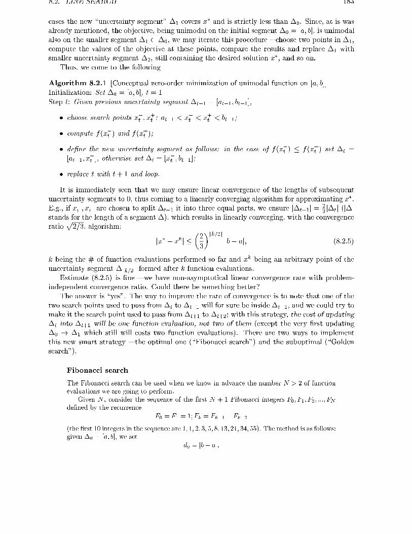
8.2. LINE SEARCH 183
cases the new \uncertainty segment" �1 covers x� and is strictly less than �0. Since, at is wasalready mentioned, the objective, being unimodal on the initial segment �0 = [a; b], is unimodalalso on the smaller segment �1 � �0, we may iterate this procedure { choose two points in �1,compute the values of the objective at these points, compare the results and replace �1 withsmaller uncertainty segment �2, still containing the desired solution x�, and so on.
Thus, we come to the following
Algorithm 8.2.1 [Conceptual zero-order minimization of unimodal function on [a; b]]Initialization: Set �0 = [a; b], t = 1Step t: Given previous uncertainty segment �t�1 = [at�1; bt�1],
� choose search points x�t ; x+t : at�1 < x�t < x+t < bt�1;
� compute f(x�t ) and f(x+t );
� de�ne the new uncertainty segment as follows: in the case of f(x�t ) � f(x+t ) set �t =[at�1; x
+t ], otherwise set �t = [x�t ; bt�1];
� replace t with t+ 1 and loop.
It is immediately seen that we may ensure linear convergence of the lengths of subsequentuncertainty segments to 0, thus coming to a linearly converging algorithm for approximating x�.E.g., if x�t ; x
+t are chosen to split �t�1 it into three equal parts, we ensure j�t+1j = 2
3 j�tj (j�jstands for the length of a segment �), which results in linearly converging, with the convergenceratio
p2=3, algorithm:
jx� � xkj ��2
3
�bk=2cjb� aj; (8.2.5)
k being the # of function evaluations performed so far and xk being an arbitrary point of theuncertainty segment �bk=2c formed after k function evaluations.
Estimate (8.2.5) is �ne { we have non-asymptotical linear convergence rate with problem-independent convergence ratio. Could there be something better?
The answer is \yes". The way to improve the rate of convergence is to note that one of thetwo search points used to pass from �t to �t+1 will for sure be inside �t+1, and we could try tomake it the search point used to pass from �t+1 to �t+2; with this strategy, the cost of updating�t into �t+1 will be one function evaluation, not two of them (except the very �rst updating�0 ! �1 which still will costs two function evaluations). There are two ways to implementthis new smart strategy { the optimal one (\Fibonacci search") and the suboptimal (\Goldensearch").
Fibonacci search
The Fibonacci search can be used when we know in advance the number N > 2 of functionevaluations we are going to perform.
Given N , consider the sequence of the �rst N + 1 Fibonacci integers F0; F1; F2; :::; FNde�ned by the recurrence
F0 = F1 = 1;Fk = Fk�1 + Fk�2
(the �rst 10 integers in the sequence are 1; 1; 2; 3; 5; 8; 13; 21; 34; 55). The method is as follows:given �0 = [a; b], we set
d0 = jb� aj;

184 LECTURE 8. OPTIMIZATION METHODS: INTRODUCTION
choose two �rst search points x�1 and x+1 at the distance
d1 =FN�1FN
d0
from the right and from the left endpoints of �0, respectively (since FN=FN�1 = (FN�1 +FN�2)=FN�1 = 1 + FN�2=FN�1 < 2, we have d1 > d0=2, so that x�1 < x+1 ). The length ofthe new uncertainty segment �1 clearly will be d1.
What we are about to do is to iterate the above step, with N replaced by N � 1. Thus,now we should evaluate f at two points x�2 ; x
+2 of the segment �1 placed at the distance
d2 =FN�2FN�1
d1 [=FN�2FN�1
FN�1FN
d0 =FN�2FN
d0] (8.2.6)
from the right and the left endpoint of �1. The crucial fact (which takes its origin in thearithmetic properties of the Fibonacci numbers) is thatone of these two required points where f should be computed is already processed { this isthe one of the previous two points which belongs to �1.
Indeed, assume, without loss of generality, that �1 = [a; x+1 ] (the case �1 = [x�1 ; b] iscompletely similar), so that the one of the �rst two search point belonging to �1 is x
�1 . We
have
x�1 � a = (b� d1)� a = (b� a)� d1 = d0 � d1 = d0
�1� FN�1
FN
�=
[since FN = FN�1 + FN�2 and d2 =FN�2FN
d0]
= d0FN�2FN
= d2:
Thus, only one of the two required points of �1 is new for us, and another comes from theprevious step; consequently, in order to update �1 into �2 we need one function evaluation,not two of them. After this new function evaluation, we are able to replace �1 with �2. Toprocess �2, we act exactly as above, but with N replaced by N�2; here we need to evaluatef at the two points of �2 placed at the distance
d3 =FN�3FN�2
d2 [=FN�3FN
d0; see (8.2.6)]
from the endpoints of the segment, and again one of these two points already is processed.Iterating this procedure, we come to the segment �N�1 which covers x�; the length of
the segment is
dN�1 =F1FN
d0 =b� a
FN;
and the total # of evaluations of f required to get this segment is N (we need 2 evaluationsof f to pass from �0 to �1 and one evaluation per every of N � 2 subsequent updatings�t 7! �t+1, 1 � t � N � 2).
Taking, as approximation of x�, any point xN of the segment �N�1, we have
jxN � x�j � j�N j = b� a
FN: (8.2.7)
To compare (8.2.7) with the accuracy estimate (8.2.5) of our initial { unsophisticated {method, note that
Ft =1
�+ 2
�(�+ 1)�t + (�1)t��t� ; � = 1 +
p5
2> 1:3) (8.2.8)
3Here is the computation: the Fibonacci numbers satisfy the homogeneous �nite-di�erence equation
xt � xt�1 � xt�2 = 0

8.2. LINE SEARCH 185
Consequently, (8.2.7) results in
jxN � x�j � �+ 2
�+ 1��N jb� aj(1 + o(1)); (8.2.9)
where o(1) denotes a function of N which converges to 0 as N !1).We see that the convergence ratio for the Fibonacci search is
��1 =2
1 +p5= 0:61803:::
which is much better than the ratiop2=3 = 0:81649::: given by (8.2.5).
It can be proved that the Fibonacci search is, in certain precise sense, the optimal,in terms of the accuracy guaranteed after N function evaluations, zero-order method forminimizing an unimodal function on a segment. In spite of this �ne theoretical property, themethod is not that convenient from the practical viewpoint: we should choose in advance thenumber of function evaluations to be performed (i.e., to tune the method to certain chosenin advance accuracy), which is sometimes inconvenient. The Golden search method we areabout to present is free of this shortcoming and at the same time is, for not too small N ,basically as eÆcient as the original Fibonacci search.
The idea of the Golden Search method is very simple: at k-th step of theN -step Fibonaccisearch, we choose two search points in the segment �k�1, and each of these points dividesthe segment (from the closer endpoint to the more far one) in the ratio
[1� FN�k=FN�k+1] : [FN�k=FN�k+1] ;
i.e., in the ratio FN�k�1 : FN�k. According to (8.2.8), this ratio, for large N � k, is close to1 : �, � = (1 +
p5)=2. In the Golden search we use this ratio at every step, and that is it!
Golden search
Let � = (1+p5)=2 (this is the so called \golden ratio") . In the Golden search implementation
of Algorithm 8.2.1 we choose at every step the search points x�t and x+t to divide the previoussegment of uncertainty �t�1 = [at�1; bt�1] in the ratio 1 : �:
x�t =�
1 + �at�1 +
1
1 + �bt�1; x+t =
1
1 + �at�1 +
�
1 + �bt�1: (8.2.10)
It is easily seen that for t � 2, one of the search points required to update �t�1 into �t isalready processed in course of updating �t�2 into �t�1. To verify it, it suÆces to considerthe case when �t�2 = [�; �] and �t�1 = [�; x+t�1] (the \symmetric" case �t�1 = [x�t�1; �] iscompletely similar). Denoting d = � � �, we have
x�t�1 = �+1
1 + �d; x+t�1 = �+
�
1 + �d; (8.2.11)
and initial conditions x0 = x1 = 1. To solve a �nite di�erence homogeneous equation, one should �rst look forits fundamental solutions { those of the type xt = �t. Substituting xt = �t into the equation, we get a quadraticequation for �:
�2 � �� 1 = 0;
and we come to two fundamental solutions:
x(i)t = �ti; i = 1; 2; with �1 =1 +
p5
2> 1; �2 = �1=�1:
Any linear combination of these fundamental solutions again is a solution to the equation, and to get fFtg, itremains to choose the coeÆcients of the combination to �t the initial conditions F0 = F1 = 1. As a result, wecome to (8.2.8). A surprise is that the expression for integer quantities Ft involves irrational number!

186 LECTURE 8. OPTIMIZATION METHODS: INTRODUCTION
now, we are in situation �t�1 = [�; x+t�1], so that the second of the two search points needed toupdate �t�1 into �t is
x+t = �+�
1 + �(x+t�1 � �) = �+
�2
(1 + �)2d
(see the second equality in (8.2.11)). The latter quantity, due to the �rst equality in (8.2.11)and the characteristic equation �2 = 1 + � giving �, is nothing but x�t�1:
�2 = 1 + �, 1
1 + �=
�2
(1 + �)2:
Thus, in the Golden search each updating �t�1 7! �t, except the very �rst one, requires a singlefunction evaluation, not two of them. The length of the uncertainty segment is reduced by everyupdating by factor
�
1 + �=
1
�;
i.e.,j�tj = ��t(b� a):
After N � 2 function evaluations (i.e., after t = N � 1 steps of the Golden search) we canapproximate x� by (any) point xN of the resulting segment �N�1, and inaccuracy bound willbe
jxN � x�j � j�N�1j � �1�N (b� a): (8.2.12)
Thus, we have the linear rate of convergence with convergence ratio ��1 = 0:61803:::, same asfor the Fibonacci search, but now the method is \stationary" { we can perform as many stepsof it as we wish.
8.2.2 Bisection
The theoretical advantage of the zero-order methods, like the Fibonacci search and the Goldensearch, is that these methods use the minimal information on the objective { its values only. Be-sides this, the methods have a very wide �eld of applications { the only requirement imposed onthe objective is to be unimodal on a given segment which localizes the minimizer to be approxi-mated. And even under these extremely mild restrictions these methods are linearly convergingwith objective-independent converging ratio; moreover, the corresponding eÆciency estimates(8.2.9) and (8.2.12) are non-asymptotical: they do not contain \uncertain" constant factors andare valid for all values of N . At the same time, typically our objective is better behaved than ageneral unimodal function, e.g., is smooth enough. Making use of these additional properties ofthe objective, we may improve the behaviour of the line search methods.
Let us look what happens if we are solving problem (8.2.2) with smooth { continuouslydi�erentiable { objective. Same as above, assume that the objective is unimodal on [a; b]. Infact we make a little bit stronger assumption:
(A): the minimizer x� of f on [a; b] is an interior point of the segment, and f 0(x) changes itssign at x�:
f 0(x) < 0; x 2 [a; x�); f 0(x) > 0; x 2 (x�; b]
[unimodality + di�erentiability imply only that f 0(x) � 0 on [a; x�) and f 0(x) � 0 on (x�; b]].

8.2. LINE SEARCH 187
Besides these restrictions on the problem, assume, as it is normally the case, that we areable to compute not only the value, but also the derivative of the objective at a given point.
Under these assumptions we can solve (8.2.2) by de�nitely the simplest possible method {the bisection. Namely, let us compute f 0 at the midpoint x1 of �0 = [a; b]. There are threepossible cases:
� f 0(x1) > 0. This case, according to (A), is possible if and only if x� < x1, and we canreplace the initial segment of uncertainty with �1 = [a; x1], thus reducing the length ofthe uncertainty segment by factor 2;
� f 0(x1) < 0. Similarly to the previous case, this inequality is possible if and only if x� > x1,and we can replace the initial segment of uncertainty with [x1; b], again reducing the lengthof the uncertainty segment by factor 2;
� f 0(x1) = 0. According to (A), it is possible if and only if x1 = x�, and we can terminatewith exact minimizer at hand.
In the �rst two cases our objective clearly possesses property (A) with respect to the new segmentof uncertainty, and we can iterate the construction. Thus, we come to
Algorithm 8.2.2 [Bisection]Initialization: set �0 = [a; b], t = 1Step t: Given previous uncertainty segment �t�1 = [at�1; bt�1],
� de�ne current search point xt as the midpoint of �t�1:
xt =at�1 + bt�1
2;
� compute f 0(xt);
� in the case of f 0(xt) = 0 terminate and claim that xt is the exact solution to (8.2.2).Otherwise set
�t =�[at�1; xt]; f 0(xt) > 0[xt; bt�1]; f 0(xt) < 0
replace t with t+ 1 and loop.
From the above considerations we immediately conclude that
Proposition 8.2.1 [Linear convergence of Bisection]Under assumption (A), for any t � 1, either the Bisection search terminates in course of the�rst t steps with exact solution x�, or t-th uncertainty segment �t is well-de�ned, covers x� andis of the length 2�t(b� a).
Thus, the Bisection method converges linearly with convergence ratio 0:5.
Remark 8.2.1 The convergence ratio of the Bisection algorithm is better than the one0.61803... for Fibonacci/Golden search. There is no contradiction with the announced optimal-ity of the Fibonacci search: the latter is optimal among the zero-order methods for minimizingunimodal functions, while Bisection is a �rst-order method.

188 LECTURE 8. OPTIMIZATION METHODS: INTRODUCTION
Remark 8.2.2 The Bisection method can be viewed as the \limiting case" of the conceptualzero-order Algorithm 8.2.1: when, in the latter algorithm, we make both the search points x�tand x+t close to the midpoint of the uncertainty segment �t�1, the result of comparison betweenf(x�t ) and f(x
+t ) which governs the choice of the new uncertainty segment in Algorithm 8.2.1
is given by the sign of f 0 at the midpoint of �t�1.
Remark 8.2.3 Note that the assumption (A) can be weakened. Namely, let us assume that f 0
changes its sign at the segment [a; b]: f 0(a) < 0, f 0(b) > 0; and we assume nothing about thederivative in (a; b), except its continuity. In this case we still can successfully use the Bisectionmethod to approximate a critical point of f in (a; b), i.e., a point where f 0(x) = 0. Indeed, fromthe description of the method it is immediately seen that what we do is generating a sequenceof nested segments �0 � �1 � �2 � :::, with the next segment being twice smaller than theprevious one, with the property that f 0 changes it sign from � to + when passing from theleft endpoint of every segment �t to its right endpoint. This process can be terminated onlyin the case when the current iterate xt is a critical point of f . If it does not happen, then thenested segments �t have a unique common point x�, and since in any neighbourhood of thepoint there are points both with positive and negative values of f 0, we have f 0(x�) = 0 (recallthat f 0 is continuous). This is the critical point of f to which the algorithm converges linearlywith convergence ratio 0:5.
The indicated remark explains the nature of the bisection algorithm. This is an algorithmfor �nding zero of the function f 0 rather than for minimizing f itself (under assumption (A), ofcourse, this is the same - to minimize f on [a; b] or to �nd the zero of f 0 on (a; b)). And theidea of the algorithm is absolutely trivial: given that the zero of f 0 is bracketed by the initialuncertainty segment �0 = [a; b] (i.e., that f 0 at the endpoints of the segment is of di�erent sign),we generate the sequence of enclosed segments, also bracketing zero of f 0, as follows: we splitthe previous segment �t = [at�1; bt�1] by its midpoint xt into two subsegments [at�1; xt] and[xt; bt�1]. Since f 0 changes its sign when passing from at�1 to bt�1, it changes its sign eitherwhen passing from at�1 to xt, or when passing from xt to bt�1 (provided that f 0(xt) 6= 0, so thatwe can speak about the sign of f 0(xt); if f 0(xt) = 0, we are already done). We detect on whichof the two subsegments f 0 in fact changes sign and take it as the new uncertainty segment �t;by construction, it also brackets a zero of f 0.
8.2.3 Curve �tting
The line search methods considered so far possess, under unimodality assumption, nice objective-independent global linear convergence. May we hope for something better? Of course, yes: itwould be �ne to get something superlinearly converging. If the objective is \well-behaved" {smooth enough { we have good chances to accelerate convergence, at least at the �nal stage,by curve �tting, i.e., by approximating the objective by a simple function with analyticallycomputable minimum. The natural way is to approximate f by a polynomial, choosing thecoeÆcients of the polynomial in order to �t it to the observed values (and derivatives, if we areable to compute these derivatives) of f at several \most perspective" iterates. An iteration of apure curve �tting algorithm is as follows:
� at the beginning of the iteration, we have certain set of \working points" where we alreadyhave computed the values and, possibly, certain derivatives of the objective. Given thesedata, we compute the current approximating polynomial p which should have the samevalues and derivatives at the working points as those of the objective

8.2. LINE SEARCH 189
� after approximating polynomial p is computed, we �nd analytically its minimizer and takeit as the new search point
� we compute the value (and, possibly, the derivatives) of the objective at the new searchpoint and update the set of working points, adding to it the last search point (along withthe information on the objective at this point) and excluding from this set the \worst" ofthe previous working points, and then loop.
The idea underlying the outlined approach is very simple: if we somehow can enforce the pro-cedure to converge, the working points will eventually be at certain small distance d from theminimizer of f . If f is smooth enough, the error in approximating f by p in the d-neighbourhoodof working points will be of order of dq+1, q being the degree of p, and the error in approximatingf 0 by p0 will be of order of dq. Consequently, we may hope that the distance from the minimizerof p (i.e., the zero of p0) to the minimizer of f (the zero of f 0) will be of order of dq, which givesus good chances for superlinear convergence.
Of course, what is said is nothing but a very rough idea. Let us look at several standardimplementations.
Newton's method
Assume that we are solving problem (8.2.1) with twice continuously di�erentiable objective f ,and that, given x, we can compute f(x), f 0(x), f 00(x). Under these assumptions we can applyto the problem the Newton method as follows:
Algorithm 8.2.3 [One-dimensional Newton method]Initialization: choose somehow starting point x0Step t: given the previous iterate xt�1,
� compute f(xt�1); f 0(xt�1); f 00(xt�1) and approximate f around xt�1 by its second-orderTaylor expansion
p(x) = f(xt�1) + f 0(xt�1)(x� xt�1) +1
2f 00(xt�1)(x� xt�1)
2;
� choose as xt the minimizer of the quadratic function p(�):
xt = xt�1 � f 0(xt�1)
f 00(xt�1);
replace t with t+ 1 and loop.
The Newton method, started close to a nondegenerate local minimizer x� of f (i.e., close to apoint x� satisfying the suÆcient second order optimality condition: f 0(x�) = 0, f 00(x�) > 0),converges to x� quadratically:
Proposition 8.2.2 [Local quadratic convergence of the Newton method]Let x� 2 R be a nondegenerate local minimizer of smooth function f , i.e., a point such that fis three times continuously di�erentiable in a neighbourhood of x� with f 0(x�) = 0, f 00(x�) > 0.Then the Newton iterates converge to x� quadratically, provided that the starting point x0 isclose enough to x�.

190 LECTURE 8. OPTIMIZATION METHODS: INTRODUCTION
Proof. Let g(x) = f 0(x), so that g(x�) = 0, g0(x�) > 0 and
xt = xt�1 � g(xt�1)
g0(xt�1):
Since g = f 0 is twice continuously di�erentiable in a neighbourhood of x� and g0(x�) > 0, thereexist positive constants k1, k2, r such that
jx0 � x�j; jx00 � x�j � r ) jg0(x0)� g0(x00)j � k1jx0 � x00j; g0(x0) � k2: (8.2.13)
Now let
� = minfr; k2k1g: (8.2.14)
Assume that for certain t the iterate xt�1 belongs to the �-neighbourhood
U� = [x� � �; x� + �]
of the point x�. Then g0(xt�1) � k2 > 0 (due to (8.2.13); note that � � r), so that the Newtoniterate xt of xt�1 is well-de�ned. We have
xt � x� = xt�1 � x� � g(xt�1)
g0(xt�1)=
[since g(x�) = 0]
xt�1 � x� � g(xt�1)� g(x�)
g0(xt�1)=g(x�)� g(xt�1)� g0(xt�1)(x� � xt�1)
g0(xt�1):
The numerator in the resulting fraction is the remainder in the �rst order Taylor expansion ofg at xt�1; due to (8.2.13) and since jxt�1� x�j � � � r, it does not exceed in absolute value thequantity 1
2k1jx� � xt�1j2. The denominator, by the same (8.2.13), is at least k2. Thus,
xt�1 2 U� ) jxt � x�j � k12k2
jxt�1 � x�j2: (8.2.15)
Due to the origin of �, (8.2.15) implies that
jxt � x�j � jxt�1 � x�j=2;we see that the trajectory of the Newton method, once reaching U�, never leaves this neigh-bourhood and converges to x� linearly with convergence ratio 0:5. It for sure is the case whenx0 2 U�, and let us specify the \close enough" in the statement of the proposition just as inclu-sion x0 2 U�. With this speci�cation, we get that the trajectory converges to x� linearly, andfrom (8.2.15) it follows that in fact the order of convergence is (at least) 2.
Remark 8.2.4 Both the assumptions that f 00(x�) > 0 and that x0 is close enough areessential4). E.g., as applied to the smooth convex function
f(x) = x4
4in fact, the assumption f 00(x�) > 0 can be replaced with f 00(x�) < 0, since the trajectory of the method remainsunchanged when f is replaced with �f (in other words, the Newton method does not distinguish between thelocal minima and local maxima of the objective). We are speaking about the case of f 00(x�) > 0, not the one off 00(x�) < 0, simply because the former case is the only important for minimization.

8.2. LINE SEARCH 191
(with degenerate minimizer x� = 0), the method becomes
xt = xt�1 � 1
3xt�1 =
2
3xt�1;
in this example the method converges, but linearly rather than quadratically.As applied to strictly convex smooth function
f(x) =p1 + x2
with unique (and nondegenerate) local (and global as well) minimizer x� = 0, the methodbecomes, as it is immediately seen,
xt = �x3t�1;this procedure converges (very fast: with order 3) to 0 provided that the starting point is in(�1; 1), and diverges to in�nity { also very fast { if jx0j > 1.
In fact the Newton method is a linearization method for �nding zero of f 0: given the previousiterate xt�1, we linearize g = f 0 at this point and take as xt the solution to the linearization
g(xt�1) + g0(xt�1)(x� xt�1) = 0
of the actual equation g(x) = 0.
f’(x)
xt
xt-1
Newton method as zero-�nding routine
Regula Falsi (False Position) method
This method, same as the Newton one, is based on approximating f by a quadratic polyno-mial, but here this polynomial is constructed via two working points with �rst-order infor-mation rather than via a single working point with second-order information. The method,in its most straightforward form, is as follows. Given two latest iterates xt�1, xt�2, alongwith the values f and f 0 at these iterates, we approximate f 00(xt�1) by the �nite di�erence
f 0(xt�1)� f 0(xt�2)
xt�1 � xt�2
and use this approximation to approximate f by a quadratic function
p(x) = f(xt�1) + f 0(xt�1)(x � xt�1) +1
2
f 0(xt�1)� f 0(xt�2)
xt�1 � xt�2(x � xt�1)
2:

192 LECTURE 8. OPTIMIZATION METHODS: INTRODUCTION
The new iterate is the minimizer of this quadratic function:
xt = xt�1 � f 0(xt�1)xt�1 � xt�2
f 0(xt�1)� f 0(xt�2): (8.2.16)
Note that although the polynomial p is chosen in asymmetric with respect to xt�1 and xt�2way (it is tangent to f at xt�1, but even not necessarily coincides with f at xt�2), theminimizer xt of this polynomial is symmetric with respect to the pair of working points; asit is immediately seen, the right hand side of (8.2.16) can be equivalently rewritten as
xt = xt�2 � f 0(xt�2)xt�1 � xt�2
f 0(xt�1)� f 0(xt�2):
The geometry of the method is very simple: same as the Newton method, this is the methodwhich actually approximates the zero of g(x) = f 0(x) (look: the values of f are not involvedinto the recurrence (8.2.16)). In the Newton method we, given the value and the derivative ofg at xt�1, approximate the graph of g by its tangent at xt�1 line g(xt�1)+g0(xt�1)(x�xt�1)and choose xt as the point where this tangent line crosses the x-axis. In the Regula Falsimethod we, given the values of g at two points xt�1 and xt�2, approximate the graph of gby the secant line passing through (xt�1; g(xt�1)) and (xt�2; g(xt�2)) and choose as xt thepoint where this secant line crosses the x-axis.
xt-1
xt-2xt
f’(x)
Regula Falsi method as zero-�nding routineThe local rate of convergence of the method is given by the following
Proposition 8.2.3 [Local superlinear convergence of Regula Falsi method]Let x� be a nondegenerate minimizer of a smooth function f , namely, a point such that f isthree times continuously di�erentiable in a neighbourhood of x� with f 0(x�) = 0, f 00(x�) > 0.Then, for starting pair x0; x1 of two distinct points close enough to x� the method convergesto x� superlinearly with order of convergence
� =1 +
p5
2:
Note that, same as for the Newton method, the assumptions of the proposition, especiallythe one of closeness of x0 and x1 to x�, are essential: badly started, the method may be

8.2. LINE SEARCH 193
non-converging:
x xx2 1 0f’(x)
x3
Cycle in Regula Falsi: the trajectory is x0; x1; x2; x3; x0; x1; :::
Cubic �t
Approximating polynomials used in curve �tting methods are of small order { not greaterthan 3, which is clear: to run the method, we should be able to compute the minimizer of apolynomial analytically. The Cubic �t is based on this \highest-order" approximation. Atthe step t of the method, given the latest two iterates x0 = xt�1 and x00 = xt�2 along withthe values of f and f 0 at the points, one de�nes the cubic polynomial p(�) such that
p(x0) = f(x0); p0(x0) = f 0(x0); p(x00) = f(x00); p0(x00) = f 0(x00)
(these are four linear equations on four coeÆcients of the polynomial; if x0 6= x00, which, aswe shall see, always can be assumed, the equations uniquely de�ne p). As the next iterate,one chooses the local minimizer of p. If exists, the minimizer is given by the relations
xt = x0 � (x0 � x00)
�u1 + u2 � f 0(x0)
f 0(x00)� f 0(x0) + 2u2
�;
u1 = f 0(x0) + f 0(x00)� 3f(x0)� f(x00)
x0 � x00; u2 =
qu21 � f 0(x0)f 0(x00): (8.2.17)
The step is for sure well-de�ned if f 0(x0) and f 0(x00) are of opposite signs (\V -shape"; com-pare with Bisection). One can prove that if x� is a nondegenerate local minimizer of asmooth enough function f , then the method, started close enough to x�, converges to x�
quadratically.
Safeguarded curve �tting
There are many other curve �tting schemes: the one based on rational approximation of theobjective, the one where the objective is approximated by a quadratic polynomial accordingto its values at three-point working set, etc. All curve �tting methods have common advan-tage: superlinear local convergence for well-behaved functions. And all these methods havecommon disadvantage as well: if the method is started far from optimum, the method candiverge (see, e.g., Remark 8.2.4). To overcome this severe shortcoming, it is recommended tocombine reliable linearly converging (in the case of unimodal objectives) methods like Goldensearch or Bisection with curve �tting. The idea is as follows. At step t of the method wehave previous uncertainty segment �t�1 = [at�1; bt�1] (f 0(xt�1) < 0, f 0(bt�1) > 0), as wellas certain working set Wt comprised of several previous iterates where we know the valuesof f and, possibly, the derivatives of f . Same as in the curve �tting methods, we

194 LECTURE 8. OPTIMIZATION METHODS: INTRODUCTION
use the working set to form polynomial (or rational) approximation p to f and computeanalytically the minimizer of p (or something close to this minimizer). In the curve �ttingmethods the resulting point, let it be called u, is used as the next iterate. In contrast tothis, in the safeguarded curve �tting it is used as the next iterate only if u is \reasonablyplaced" with respect to �t�1; if it is not the case, the next iterate is chosen according to theBisection/Golden search scheme, depending on whether we use the derivatives of f .
The notion of a \reasonably placed" u contains several tests. First of all, u should bewell-de�ned and belong to �t�1, but this is not all. It is recommended, e.g., not to useu if it is too far from the best (with the smallest value of f) point of the working set,say, is at the distance larger than 1
2 j�t�1j (since in this case the Bisection step is likely toreduce inaccuracy better than the curve �tting one). After the step { the curve �tting orthe \safeguarding" (Bisection/Golden search) one { is performed, one updates the workingset and the uncertainty segment.
Of course, what is said is not a description of a concrete method, but a very rough idea
which admits many implementations (detailed speci�cation of which curve �tting method to
use, what is a \reasonably placed" u, rules for updating the working set, etc.) With good im-
plementation, the safeguarded curve �tting combines the advantages of the Bisection/Golden
search (global linear convergence with objective-independent rate in the unimodal case) and
those of curve �tting (superlinear local convergence for well-behaved objectives).
8.2.4 Inexact Line Search
As it was already mentioned, the main application of line search methods is inside algorithmsfor multi-dimensional optimization. In these algorithms we always allow only small numberof steps of the line search subroutine at each iteration of the master algorithm, otherwise theoverall complexity of the master method will be too large. Moreover, in many multidimensionalalgorithms we are not that interested in high-accuracy solutions of one-dimensional subproblems;what is crucial for the master method, is reasonable progress in solving these subproblems.Whenever it is the case, we can terminate line search relatively far from the actual solution ofthe subproblem in question, using certain simple tests for \reasonable progress". Let us describetwo most popular tests of this type.
Armijo's rule
Consider the situation which is typical for application of line search technique inside multi-dimensional master method. At an iteration of the latter method we have current iterate x 2Rn and search direction d 2 Rn which is a descent direction for our multivariate objectivef(�) : Rn ! R:
dTrf(x) < 0: (8.2.18)
The goal is to reduce \essentially" the value of the objective by a step
x 7! x+ �d
from x in the direction d.Assume that f is continuously di�erentiable. Then the function
�( ) = f(x+ d)
of one variable also is once continuously di�erentiable; moreover, due to (8.2.18), we have
�0(0) < 0;

8.2. LINE SEARCH 195
so that for small positive one has
�( )� �(0) � �0(0) < 0:
Our desire is to choose a \`reasonably large" stepsize � > 0 which results in the progress�( �) � �(0) in the objective \of order of ��0(0)". The Armijo test for this requirement is asfollows:
Armijo's Test:we �x once for ever constants � 2 (0; 1) (popular choice is � = 0:2) and � > 1 (say, � = 2 or� = 10) and say that candidate value > 0 is appropriate, if the following two relations aresatis�ed:
�( ) � �(0) + � �0(0) (8.2.19)
[this part of the test says that the progress in the value of � given by the stepsize is \of orderof �0(0)"]
�(� ) � �(0) + �� �0(0) (8.2.20)
[this part of the test says that is \maximal in order" stepsize which satis�es (8.2.19) { if wemultiply by �, the increased value fails to satisfy (8.2.19), at least to satisfy it as a strictinequality]
Under assumption (8.2.18) and the additional (very natural) assumption that f (and, conse-quently, �) is below bounded, the Armijo test is consistent: there do exist values of > 0 whichpass the test. To see it, it suÆces to notice that
A. (8.2.19) is satis�ed for all small enough positive .Indeed, since � is di�erentiable, we have
0 > �0(0) = lim !+0
�( )� �(0)
;
whence
��0(0) � �( ) � �(0)
for all small enough positive (since ��0(0) > �0(0) due to �0(0) < 0; � 2 (0; 1)); the resultinginequality is equivalent to (8.2.19);
B. (8.2.19) is not valid for all large enough values of .Indeed, the right hand side of (8.2.19) tends to �1 as ! 1, due to �0(0) < 0, and the lefthand side is assumed to be below bounded.
Now let us choose an arbitrary positive = 0 and test whether it satis�es (8.2.19). If it isthe case, let us replace this value subsequently by 1 = � 0, 2 = � 1, etc., each time verifyingwhether the new value of satis�es (8.2.19). According to B, this cannot last forever: for certains � 1 s for sure fails to satisfy (8.2.19). When it happens for the �rst time, the quantity s�1turns out to satisfy (8.2.19), while the quantity s = � s�1 fails to satisfy (8.2.19), which meansthat = s�1 passes the Armijo test.
If the initial 0 does not satisfy (8.2.19), we replace this value subsequently by 1 = ��1 0, 2 = ��1 1, etc., each time verifying whether the new value of still does not satisfy (8.2.19).According to A, this cannot last forever: for certain s � 1, s for sure satis�es (8.2.19). Whenit happens for the �rst time, s turns out to satisfy (8.2.19), while s�1 = � s fails to satisfy(8.2.19), and = s passes the Armijo test.

196 LECTURE 8. OPTIMIZATION METHODS: INTRODUCTION
Note that the presented proof in fact gives an explicit (and fast) algorithm for �nding astepsize passing the Armijo test, and this algorithm can be used (and often is used) in Armijo-aimed line search instead of more accurate (and normally more time-consuming) line searchmethods from the previous sections.
Goldstein test
Another popular test for \suÆcient progress" in line search is as follows:
Goldstein test:
we �x one for ever constant � 2 (0; 1=2) and say that candidate value > 0 is appropriate, if
�(0) + (1� �) �0(0) � �( ) � �(0) + � �0(0): (8.2.21)
Here again relation (8.2.16) and below boundedness of f imply consistency of the test.

8.2. LINE SEARCH 197
Assignment # 8 (Lecture 8)
Exercise 8.1 [Golden search] Write a code implementing the Golden search and run it onseveral unimodal test functions on your choice.
Exercise 8.2 [Bisection] Write a code implementing the Bisection and run it on several uni-modal test functions on your choice.
Run 50 steps of the Bisection algorithm on the (non-unimodal) function
f(x) = � sin
2�
217 + x
![x � 0]
with the initial uncertainty segments (a) [0; 1]; (b) [0; 4], taking as the result the midpoint of the�nal uncertainty segment. Why the results are di�erent?
Exercise 8.3 [Golden search vs Bisection] Assume that the problem (8.2.2) to be solved satis�esassumption (A) (Section 8.2.2), and that the derivatives of the objective are available. Whatshould be preferred { the Golden search or the Bisection?
Of course, Bisection has better convergence (convergence ratio 0.5 versus 0.618... for theGolden search), but this comparison is unfair: the Golden search does not use derivatives, andswitching o� the part of the code which computes f 0, normally, save the overall computationtime, in spite of larger # of steps required in Golden search to achieve the same accuracy.
The actual reason to prefer Bisection is that this method, normally, is more numericallystable. Indeed, assume that we are solving (8.2.2) and everything { the values of f; f 0; f 00 in[a; b], same as a and b themselves, are \normal reals" { those of order of 1. And assume that weare interested in reducing the initial uncertainty segment to the one of length �. What are theaccuracies � we can achieve in actual computations with their rounding errors?
The rough reasoning is as follows: to run the Golden search, we should compare values ofthe objective, at the �nal steps { at points at the distance O(�) from the minimizer. At thesepoints, the values of f di�er from the optimal value (and, consequently, from each other) byO(�2). In order to ensure correct comparison of the values (and an incorrect one may make allthe subsequent computations senseless), the absolute inaccuracy �� of machine representation ofa number of order of 1 (for double precision Fortran/C computations �� is something like 10�16)should be less than the above O(�2). Thus, the values of � we indeed can achieve in Goldensearch should be of order of O(
p��).
In the Bisection method, we should compare the values of f 0 with 0; if all intermediate resultsin the code computing the derivative are of order of 1, the derivative is computed with absoluteinaccuracy � c��, with certain constant c. If f 00(x�), x� being the minimizer of f on [a; b], ispositive of order of 1 (\the minimizer is numerically well-conditioned"), then at the distance� C� away from x� the actual values of f 0 are, in absolute values, at least C 0�, C 0 being certainconstant. We see that if x is at the distance � away from x� and � is such that C 0� > c�� (i.e.,the magnitude of f 0(x) is greater than the absolute error in computing f 0(x)), then the sign ofthe actually computed f 0(x) will be the same as the exact sign of f 0(x), and the bisection stepwill be correct. Thus, under the above assumptions we can expect that the Bisection will beable to reach accuracy � = c(C 0)�1�� = O(��) (compare with O(
p��) for the Golden search).
In order to test this reasoning, I run the Golden search and the Bisection on the problem
f(x) = (x+ 1)2 ! min j �2 � x � 1:

198 LECTURE 8. OPTIMIZATION METHODS: INTRODUCTION
To my surprise (I am inexperienced in error analysis!), both the methods solved the problemwithin accuracy of order of 10�16. After a short thought, I realized what was wrong and wasable to update the objective to observe the outlined phenomenon.
Could youa) Guess what goes wrong with the indicated example?b) Correct the example and observe the phenomenon?
Exercise 8.4 [Newton's method] Run the Newton minimization method at the functions1) f(x) = 1
2x2 � x� 1
2 expf�2xg (starting point 0:5)2) f(x) = x4 expf�x=6g (starting point 1:0)
Exercise 8.5 It was explained in the lecture that the main source of univariate optimizationproblems are line search subroutines in methods for solving multidimensional unconstrainedproblems
(f) f(x)! min j x 2 Rn:
It was also explained what is the standard situation here: given a point x and a direction dwhich is descent for f at the point (dTrf(x) < 0), we would like to carry out minimization ofthe function
�(s) = f(x+ sd)
on the nonnegative ray fs � 0g. Note that since d is descent for f , we have
�0(0) < 0:
Now, what does it mean \to carry out minimization of �", it depends on the method in question.In many (not all!) cases it would be �ne to �nd the global solution s� to the optimization problem
�(s)! min j s � 0;
provided that it exists (to this end it clearly suÆces to assume that �(s)!1 as s!1; fromnow on we assume that it indeed is the case). The diÆculty, however, is that we do not knowhow to �nd eÆciently global solutions even to one-dimensional optimization problems. In somemethods (e.g., in the Gradient Descent and the Newton ones) it suÆces to ensure \signi�cantprogress" in the objective value, and to this end one may use the Armijo line search. There are,however, methods (e.g., the Conjugate Gradient ones) which impose more restrictions on theresult s� of the search: it should satisfy both the requirement of \progress in the objective"
(a) �(s�) < �(0)
and be \nearly critical" point of �:
(b) j�0(s�)j � �;
where � > 0 is a given small tolerance. Note that (b) is \�-version" of the Fermat rule �0 = 0.It is not diÆcult to satisfy (a) and (b) separately { (a) is ensured by, say, the Armijo line
search, and (b) is ensured by Bisection { if we are clever enough to �nd a point �s > 0 such that�0(�s) > 0, we could use the Bisection on the segment [0; �s] (where �0 changes its sign from - to+) in order to approximate zero of �0. The diÆculty, however, is that in this latter routine the

8.2. LINE SEARCH 199
zero of �0 we shall �nally approach, let it be called s�, should not necessarily satisfy (a) (lookat the picture below).
b aIn this example, �s = a. Bisection will terminate with s� = b, while �(s�) > �(0).
Exercise: invent and implement in a code a \fast" linesearch routine (as fast as Bisection) whichensures both (a) and (b).
Warning: please read the text below only after you invent (or spent enough time inthinking and failed to invent) the required routine! I never have read a \canonical" solutionto the problem in books and am interested to compare your solutions with my own!
Here is my solution.Let us start with the Armijo linesearch; this is a fast routine which will result in a point, letit be called s0 > 0, which passes the Armijo test; in particular, �(s0) < �(0). I shall assumefor the sake of de�niteness that
(!) �0(s0) � 0
and strongly believe that you are able to modify by yourself the below construction for thecase of �0(s0) > 0.What I am about to do is to generate a sequence si which \quickly" { as in Bisection {converges to a zero s� of �0 and at the same time is such that �(si) � �(s0); thus, I canchoose as the point satisfying (a) and (b) the �rst point of my sequence where j�0(si)j < �(such a point exists, since si converge to a zero of �0 and �0 of course is assumed to becontinuous).
To build the sequence fsig, let us call a segment [a; b], 0 < a < b, normal, if
� �0(a) � 0
and
� or �0(b) � 0, or �(b) > �(a), or both.
My basic observation is as follows:(*) Assume that we are given a normal segment [a; b] and have computed �(c) and �0(c),c = (a + b)=2 being the midpoint of the segment. Then at least one of the two segments[a; c], [c; b] also is normal and is such that at its left endpoint � is not greater than at thepoint a. This segment is
� [a; c], if �0(c) � 0;
� [a; c], if �0(c) < 0 and �(c) > �(a);
� [c; b], if �0(c) < 0 and �(c) � �(a).
Now let us act as follows. First, let us �nd a normal segment which starts at the point s0.
To this end we test sequentially the candidate right endpoints s0 +�, s0 + 2�, s0 + 4�,...,
� > 0 being parameter of the method (I would advice to take � = s0) until the segment
[s0; s0 + 2k�] turns out to be normal; that it will happen, it is ensured by the fact that

200 LECTURE 8. OPTIMIZATION METHODS: INTRODUCTION
�(s) ! 1 as s ! 1. After we have found a normal segment of the form [s0; �s], we use (*)
to generate, starting with this segment, a sequence of \nested" normal segments, the next
being twice smaller than the previous one; fsig is exactly the sequence of the left endpoints
of these normal segments. Since the segments are nested and their lengths converge to 0,
they have a unique common point s�, and si converge to s� linearly with the convergence
ratio 1=2 { as in Bisection; according to (*), we also have �(s0) � �(s1) � :::, as it was
claimed. The only fact which should be proved is that s� is a zero of �0, but it is evident:
on every normal segment �0 takes both nonpositive and nonnegative values (indeed, it is
evident if the segment [a; b] is normal due to �0(a) � 0, �0(b) � 0; the only other possibility
for the segment to be normal is to have �0(a) � 0 and �(b) > �(a), but then [a; b] for sure
contains points with positive derivative of �, while �0(a) is nonpositive). It follows that
�0(s�) must be zero { otherwise �0, which is assumed to be continuous, would be of �xed
sign in a neighbourhood of s�, and this neighbourhood contains all normal segments from
our sequence, except �nitely many of them.

Lecture 9
Gradient Descent and Newton'sMethod
Starting from this lecture, we shall speak about methods for solving unconstrained multidimen-sional problems
f(x)! min j x 2 Rn: (9.0.1)
From now on, let us make the following assumptions:
� (A) the objective f in (9.0.1) is continuously di�erentiable;
� (B) the problem in question is solvable: the set
X� = ArgminRn
f
is nonempty.
9.1 Gradient Descent
This section is devoted to the oldest and most widely known method for (9.0.1) - the GradientDescent.
9.1.1 The idea
The idea of the method is very simple. Assume that we are at certain point x, and that we havecomputed f(x) and rf(x). Assume that x is not a critical point of f : rf(x) 6= 0 (this is thesame as to say that x is not a Karush-Kuhn-Tucker point of the problem). Then g = �rf(x)is a descent direction of f at x:
d
d j =0f(x� rf(x)) = �jrf(x)j2 < 0;
moreover, this is the best among the descent directions h (normalized to have the same lengthas that one of g) of f at x: for any h, jhj = jgj, one has
d
d j =0f(x+ h) = hTrf(x) � �jhjjrf(x)j = �jrf(x)j2
201

202 LECTURE 9. GRADIENT DESCENT AND NEWTON'S METHOD
(we have used the Cauchy inequality), the inequality being equality if and only if h = g.The indicated observation demonstrates that in order to improve x { to form a new point
with smaller value of the objective { it makes sense to perform a step
x 7! x+ g � x� rf(x)from x in the antigradient direction; with properly chosen stepsize > 0, such a step will forsure decrease f . And in the Gradient Descent method, we simply iterate the above step. Thus,the generic scheme of the method is as follows
Algorithm 9.1.1 [Generic Gradient Descent]Initialization: choose somehow starting point x0 and set t = 1Step t: at the beginning of step t we have previous iterate xt�1. At the step we
� compute f(xt�1) and rf(xt�1);� choose somehow a positive stepsize t, set
xt = xt�1 � trf(xt�1); (9.1.1)
replace t with t+ 1 and loop.
Thus, the generic Gradient Descent method is the recurrence (9.1.1) with certain rule for choos-ing stepsizes t > 0; normally, the stepsizes are given by a kind of line search applied to theunivariate functions
�t( ) = f(xt�1 � rf(xt�1)):
9.1.2 Standard implementations
Di�erent versions of line search result in di�erent versions of the Gradient Descent method.Among these versions, one should mention
� ArD [Gradient Descent with Armijo-terminated line search]: the stepsize t > 0 at itera-tion t where rf(xt�1) 6= 0 is chosen according to the Armijo test (Section 8.2.4):
f(xt�1 � trf(xt�1)) � f(xt�1)� � tjrf(xt�1)j2;f(xt�1 � � trf(xt�1)) � f(xt�1)� �� tjrf(xt�1)j2; (9.1.2)
� 2 (0; 1) and � > 1 being the parameters of the method. And if xt�1 is a critical pointof f , i.e., rf(xt�1) = 0, the choice of t > 0 is absolutely unimportant: independently ofthe value of t, (9.1.1) will result in xt = xt�1.
� StD [Steepest Descent]: t minimizes f along the ray fxt�1 � rf(xt�1) j � 0g : t 2 Argmin
�0f(xt�1 � rf(xt�1)): (9.1.3)
Of course, the Steepest Descent is a kind of idealization: in nontrivial cases we are unable tominimize the objective along the search ray exactly. Moreover, to make this idealization valid,we should assume that the corresponding steps are well-de�ned, i.e., that
Argmin �0
f(x� rf(x)) 6= ;

9.1. GRADIENT DESCENT 203
for every x; in what follows, this is assumed \by default" whenever we are speaking about theSteepest Descent.
In contrast to the Steepest Descent, the Gradient Descent with Armijo-terminated line searchis quite \constructive" { we know from Section 8.2.4 how to �nd a stepsize passing the Armijotest.
9.1.3 Convergence of the Gradient Descent
General Convergence Theorem
We start with the following theorem which establishes, under very mild restrictions, globalconvergence of the Gradient Descent to the set of critical points of f { to the set
X�� = fx 2 Rn j rf(x) = 0g:Theorem 9.1.1 [Global convergence of Gradient Descent] For both StD and ArD , the fol-lowing statements are true:
(i) If the trajectory fxtg of the method is bounded, then the trajectory possesses limitingpoints, and all these limiting points are critical points of f ;
(ii) If the level setS = fx 2 Rn j f(x) � f(x0)g
of the objective is bounded, then the trajectory of the method is bounded (and, consequently, allits limiting points, by (i), belong to X��).
Proof. (ii) is an immediate consequence of (i), since both ArD and StD clearly are descentmethods:
xt 6= xt�1 ) f(xt) < f(xt�1): (9.1.4)
Therefore the trajectory, for each of the methods, is contained in the level set S; since underassumption of (ii) this set is bounded, the trajectory also is bounded, as claimed in (ii).
It remains to prove (i). Thus, let the trajectory fxtg be bounded, and let x� be a limitingpoint of the trajectory; we should prove that rf(x�) = 0. Assume, on contrary, that it is not thecase, and let us lead this assumption to a contradiction. The idea of what follows is very simple:since rf(x�) 6= 0, a step of the method taken from x� reduces f by certain positive amount Æ;this is absolutely clear from the construction of the step. What is very likely (it should, of course,be proved, and we shall do it in a while) is that there exists a small neighbourhood U of x� suchthat a step of the method taken from arbitrary point x 2 U also improves the objective at leastby �xed positive quantity Æ0. It is absolutely unimportant for us what is this Æ0; all we need is toknow that this quantity is positive and is independent of the particular choice of x 2 U . Assumethat we already have proved that the required U and Æ0 exist. With this assumption, we get thedesired contradiction immediately: since x� is a limiting point of the trajectory, the trajectoryvisits U in�nitely many times. Each time it visits U , the corresponding step decreases f at leastby Æ0 > 0, and no step of the method increases the objective. Thus, in course of running themethod we in�nitely many times decrease the objective by Æ0 and never increase it, so that theobjective must diverge to �1 along our trajectory; the latter is impossible, since the objectivewas assumed to be below bounded.
Now it is time to prove our key argument { the one on existence of the above U and Æ0. Letme stress why there is something to be proved, in spite of the already known to us descentness ofthe method { the fact that the objective is improved by every step taken from a non-critical point
204 LECTURE 9. GRADIENT DESCENT AND NEWTON'S METHOD
of f (and all points close enough to non-critical x� also are noncritical, since rf is continuous).The diÆculty is that the progress in f in course of a step depends on from which point the stepis taken; in principle it might happen that a step from every point from a neighbourhood of x�
improves the objective, but there is no independent of the point positive lower bound Æ0 for theimprovements. And in the above reasoning we indeed require \point-independent" progress {otherwise it might happen that subsequent visits of U by the trajectory result in smaller andsmaller improvements in f , and the sum of these improvements is �nite; this possibility wouldkill the above reasoning completely.
In fact, of course, the required U; Æ0 exist. It suÆces to prove this statement for ArD only{ it is absolutely clear that the progress in the objective in course of a step of StD is at leastthe one for a step of ArD , both steps being taken from the same point. The proof for the caseof ArD looks as follows:
Since f is continuously di�erentiable and rf(x�) 6= 0, there exist positive r, P and psuch that
jx� x�j < r ) p � jrf(x)j � P ;
by the same reasons, there exists r0 2 (0; r) such that in the r0-neighbourhood V of x� onehas
jrf(x0)�rf(x00)j � � � (1� �)P�1p2:
Let U be r0=2-neighbourhood of x�. I claim that
(*) whenever x 2 U , the stepsize sx given by the Armijo line search as applied to the function
�x(s) = f(x� srf(x)) [�0x(0) = �jrf(x)j2]is at least
s� =1
2r0��1P�1:
Note that (*) is all we need. Indeed, the progress in the objective in the Armijo line searchas applied to a function � and resulting in a stepsize s is at least �sj�0(0)j. Applying thisobservation to a step of ArD taken from a point x 2 U and using (*), we come to theconclusion that the progress in the objective at the step is at least �s�jrf(x)j2 � �s�p2,and the latter quantity (which is positive and is independent of x 2 U) can be taken as thedesired Æ0.
It remains to prove (*), which is immediate: assuming that x 2 U , sx < s�, and takinginto account the construction of the Armijo test, we would get
�x(�sx)� �x(0) > ��sx�0(0): (9.1.5)
Now, since sx < s�, the segment [x; x � �sxrf(x)] is of the length at most �s�P � r0=2,and since one endpoint of the segment belongs to U , the segment itself belongs to V . Con-sequently, the derivative of f along the segment varies at most by �, so that the derivativeof � varies on the segment [0; �sx] at most by
jrf(x)j� � P� = (1� �)p2:
On the other hand, from the Lagrange Mean Value Theorem it follows that
�(�sx)� �(0) = �sx�0(�) � �sx�
0(0) + �sx(1� �)p2;
here � is some point on the segment [0; �sx]. Combining this inequality with (9.1.5), we cometo
�sx(1� �)p2 > �(1� �)�sx�0(0) � (1� �)�sxjrf(x)j2 � (1� �)�sxp
2;
which is a contradiction.
9.1. GRADIENT DESCENT 205
Please pay attention to the above proof: it structure is typical for convergence proofs intraditional Optimization and looks as follows. We know in advance that the iterative process inquestion possesses certain Lyapunov function L { one which decreases along the trajectory of theprocess and is below bounded (in the above proof this function is f itself); we also either assumethat the trajectory is bounded, or assume boundedness of the level set of the Lyapunov function,the set being associated with the value of the function at the initial point of the trajectory (then,of course, the trajectory for sure is bounded { since the Lyapunov function never decreases alongthe trajectory, the latter is unable to leave the aforementioned level set). Now assume that thethree entities { (1) the Lyapunov function, (2) our iterative process, and (3) the set X� we agreeto treat as the solution set of our problem { are linked by the following relation:
(**) if a point on the trajectory does not belong to X�, then the step of theprocess from this point strictly decreases the Lyapunov function
Normally (**) is evident from the construction of the process and of the Lyapunov function;e.g., in the above proof where L is the objective, the process is ArD or StD and X� is the setof critical points of the objective, you should not work hard in order to prove that the step froma non-critical point somehow decreases the objective. Now, given all this, we are interested toprove that the trajectory of the process converges to X�; what is the main point of the proof?Of course, an analogy of (*), i.e., a \locally uniform" version of (**) { we should prove that apoint not belonging to X� possesses a neighbourhood such that whenever the trajectory visitsthis neighbourhood, the progress in the Lyapunov function at the corresponding step is boundedaway from zero. After we have proved this crucial fact, we can immediately apply the schemeof the above proof to demonstrate that the trajectory indeed converges to X�.
I had a good reason to invest that many e�ort in explaining the \driving forces" of theabove convergence proof: from now on, I shall skip similar proofs, since I believe that the readerunderstands the general principle, and the technicalities are of minor interest here. I hope thatnow it becomes clear why in the Armijo test we require the stepsize to be the largest one (up tofactor �) resulting in \signi�cant " progress in the objective. If we would skip this \maximality"requirement, we would allow arbitrarily small stepsizes even from the points which are far fromthe solution set; as a result, (*) would not be the case anymore, and we would become unableto ensure convergence of the process (and this property indeed may be lost).
Limiting points of Gradient Descent
We have proved that the standard versions of the Gradient Descent, under the assumption thatthe trajectory is bounded, converge to the set X�� of critical points of the objective. This setfor sure contains the set X� of global minimizers of f , same as the set of local minimizers of theobjective, but this is not all: X�� contains also all local maximizers of f and the saddle points ofthe function, if any exists. An important question is whether a limiting point of the trajectoryof the Gradient Descent can be something we are not interested in { a critical point which isnot a local minimizer of the objective. What can be said is the following: a nondegenerate localmaximizer x� of f (i.e., a critical point of f such that f 00(x�) is negative de�nite) cannot be alimiting point of the trajectories of ArD and StD , excluding the case when the x� happens tobe a point of the trajectory; this may happen in ArD (although it is \practically impossible"),and it never happens in StD , except the trivial (and also \practically impossible") case whenthe trajectory is started at x�. And, speaking informally, it is \very unlikely" that a limitingpoint of the trajectory is a saddle point of the objective. Thus, \in practice" limiting points ofthe trajectory of Gradient Descent are local minimizers of the objective.

206 LECTURE 9. GRADIENT DESCENT AND NEWTON'S METHOD
9.1.4 Rates of convergence
Rate of global convergence: general C1;1 case
As we already know, under the assumption of item (ii) of Theorem 9.1.1 (i.e., when the levelset S = fx j f(x) � f(x0)g is bounded), the versions of the Gradient Descent mentioned inthe Theorem converge to the set X�� of critical points of f . What can be said about the non-asymptotical rate of convergence? The answer depends on how we measure the inaccuracy. Ifwe use to this purpose something like the distance
dist(x;X��) = miny2X��
jy � xj
from an approximate solution x to X��, no nontrivial eÆciency estimates can be established: theconvergence of the quantities dist(xt;X��) to 0 can be arbitrarily slow, even when f is convex.There is, however, another accuracy measure,
�f (x) = jrf(x)j2;
more suitable for our purposes. Note that the set X�� towards which the trajectory converges isexactly the set where �f (�) = 0, so that �f (x) indeed can be viewed as something which measuresthe \residual in the inclusion x 2 X��". And it turns out that we can point out the rate atwhich this residual converges to 0:
Proposition 9.1.1 [Non-asymptotical rate of convergence of Gradient Descent]Assume that the objective f is a C1;1 function, i.e., it is continuously di�erentiable with Lipschitzcontinuous gradient:
jrf(x)�rf(y)j � Lf jx� yj; 8x; y 2 Rn: (9.1.6)
Then for any integer N > 0:(i) For the started at x0 trajectory fxtg of StD one has
�f [t] � min0�t<N
jrf(xt)j2 � 2LfN
[f(x0)�min f ]: (9.1.7)
(ii) For the started at x0 trajectory fxtg of ArD one has
�f [t] � min0�t<N
jrf(xt)j2 � �Lf2�(1 � �)N
[f(x0)�minf ]; (9.1.8)
� 2 (0; 1), � > 1 being the parameters of the underlying Armijo test.
Proof.
10. Let us start with the following simple
Lemma 9.1.1 Under assumption of the Theorem one has
f(y) � f(x) + (y � x)Trf(x) + Lf2jy � xj2; 8x; y 2 Rn: (9.1.9)
Proof of Lemma. Let �( ) = f(x + (y � x)). Note that � is continuously di�erentiable(since f is) and
j�0(�) � �0(�)j = j(y � x)T (rf(x+ �(y � x))�rf(x+ �(y � x))j �

9.1. GRADIENT DESCENT 207
[Cauchy's inequality]
� jy � xjjrf(x + �(y � x)) �rf(x+ �(y � x))j �[(9.1.6)]
� jy � xj2Lf j�� �j:Thus,
j�0(�)� �0(�)j � Lf jy � xj2j�� �j; 8�; � 2 R: (9.1.10)
We have
f(y)� f(x)� (y � x)Trf(x) = �(1)� �(0)� �0(0) =
Z 1
0�0(�)d� � �0(0) =
=
Z 1
0[�0(�)� �0(0)]d� �
[see (9.1.10)]
�Z 1
0jy � xj2Lf�d� =
Lf2jy � xj2;
as required in (9.1.9).20. Now we are ready to prove (i). By construction of the Steepest Descent,
f(xt) = min �0
f(xt�1 � rf(xt�1)) �
[by Lemma 9.1.1]
� min �0
�f(xt�1) + [� rf(xt�1)]Trf(xt�1) + Lf
2j rf(xt�1)j2
�=
= f(xt�1) + jrf(xt�1)j2min �0
�� + Lf
2 2�= f(xt�1)� 1
2Lfjrf(xt�1)j2:
Thus, we come to the following important inequality:
f(xt�1)� f(xt) � 1
2Lfjrf(xt�1)j2 (9.1.11)
{ the progress in the objective at a step of Steepest Descent is at least of order of the squarednorm of the gradient at the previous iterate.
To conclude the proof, it suÆces to note that, due to the monotonicity of the method,the total progress in the objective in course of certain segment of steps cannot be more thanthe initial residual f(x0) � min f in the objective value; consequently, in a long segment,there must be a step with small progress, i.e., with small norm of the gradient. To make thisreasoning quantitative, let us take sum of inequalities (9.1.11) over t = 1; :::; N , coming to
1
2Lf
N�1Xt=0
jrf(xt)j2 � f(x0)� f(xN ) � f(x0)�min f:
The left hand side here is � N2Lf
min0�t<N jrf(xt)j2, and (9.1.7) follows.
30. The proof of (ii) is a little bit more involved, but follows the same basic idea: the progressat a step of ArD can be small only if the gradient at the previous iterate is small, and theprogress at certain step from a long segment of the steps must be small, since the totalprogress cannot be larger than the initial residual. Thus, in a long segment of steps we mustpass through a point with small norm of the gradient.

208 LECTURE 9. GRADIENT DESCENT AND NEWTON'S METHOD
The quantitative reasoning is as follows. First of all, progress in the objective at a stept of ArD is not too small, provided that both t and jrf(xt�1)j2 are not too small:
f(xt�1)� f(xt) � � tjrf(xt�1)j2; (9.1.12)
this is immediate consequence of the �rst inequality in (9.1.2). Second, t is not too small.Indeed, by Lemma 9.1.1 applied with x = xt�1; y = xt�1 � � trf(xt�1) we have
f(xt�1 � � trf(xt�1)) � f(xt�1)� � tjrf(xt�1)j2 + Lf2�2 2t jrf(xt�1)j2;
while by the second inequality in (9.1.2)
f(xt�1 � � trf(xt�1)) � f(xt�1)� �� tjrf(xt�1)j2:
Combining these inequalities, we get
(1� �)� tjrf(xt�1)j2 � Lf2�2 2t jrf(xt�1)j2:
Since t > 0, in the case of rf(xt�1) 6= 0 we obtain
t � 2(1� �)
�Lf; (9.1.13)
in the case of rf(xt�1) = 0 t, as we remember, can be chosen in arbitrary way withoutin uencing the trajectory (the latter in any case will satisfy xt�1 = xt = xt+1 = :::), and wemay assume that t always satis�es (9.1.13).
Combining (9.1.12) and (9.1.13), we come to the following inequality (compare with(9.1.11):
f(xt�1)� f(xt) � 2�(1� �)
�Lfjrf(xt�1)j2: (9.1.14)
Now the proof can be completed exactly as in the case of the Steepest Descent.
Remark 9.1.1 The eÆciency estimate of Proposition 9.1.1 gives sublinearly converging to 0non-asymptotical upper bound on the inaccuracies �f (�) of the iterates. Note, anyhow, that thisis a bound on the inaccuracy of the best (with the smallest norm of the gradient) of the iteratesgenerated in course of the �rst N steps of the method, not on the inaccuracy of the last iteratexN (the quantities jrf(xt)j2 may oscillate, in contrast to the values f(xt) of the objective).
Rate of global convergence: convex C1;1 case
Theorem 9.1.1 says that under mild assumptions the trajectories of ArD and StD converge tothe set X�� of critical points of f . If we assume, in addition, that f is convex, so that the setof critical points of f is the same as the set of global minimizers of the function, we may claimthat the trajectories converge to the optimal set of the problem. Moreover, in the case of convexC1;1 objective (see Proposition 9.1.1) we can get non-asymptotical eÆciency estimates in termsof the residuals f(xt) � min f , and under additional nondegeneracy assumption (see below) {also in terms of the distances jxt � x�j from the iterates to the optimal solution.
To simplify our considerations and to make them more \practical", in what follows we restrictourselves with the Armijo-based version ArD of the Gradient Descent.

9.1. GRADIENT DESCENT 209
Convex C1;1 case:
Proposition 9.1.2 [Rate of global convergence of ArD in convex C1;1 case]Let the parameter � in the ArD method be � 0:5, and let f be a convex C1;1 function with anonempty set X� of global minimizers. Then
(i) The trajectory fxtg of ArD converges to certain point x� 2 X�;(ii) For every N � 1 one has
f(xN )�min f � �Lf dist2(x0; x�)
4(1� �)N; (9.1.15)
where Lf is the Lipschitz constant of rf(�) and
dist(x;X�) = miny2X�
jy � xj: (9.1.16)
Proof.
10. Let x� be a point from X�, and let us look how the squared distances
d2t = jxt � x�j2
vary with t. We have
d2t = jxt � x�j2 � j[xt�1 � trf(xt�1)]� x�j2 = j[xt�1 � x�]� trf(xt�1)j2 == jxt�1 � x�j2 � 2 t(xt�1 � x�)Trf(xt�1) + 2t jrf(xt�1)j2: (9.1.17)
Since f is convex, from the Gradient Inequality
f(y) � f(x) + (y � x)Trf(x) 8x; y 2 Rn
it follows that
(xt�1 � x�)Trf(xt�1) � f(xt�1)� f(x�) = f(xt�1)�min f:
This inequality combined with (9.1.17) results in
d2t � d2t�1 � t�2�t�1 � tjrf(xt�1)j2
�; �s � f(xs)�min f � 0: (9.1.18)
According to (9.1.12), we have
tjrf(xt�1)j2 � 1
�[f(xt�1)� f(xt)] =
1
�[�t�1 � �t]:
Combining this inequality with (9.1.18), we get
d2t � d2t�1 � t�(2� ��1)�t�1 + ��1�t
�: (9.1.19)
Since, by assumption, 1=2 � �, and clearly �s � 0, the quantity in the parentheses in theright hand side is nonnegative. We know also from (9.1.13) that
t � � =2(1� �)
�Lf;
so that (9.1.19) results in
d2t � d2t�1 � � �(2� ��1)�t�1 + ��1�t
�: (9.1.20)

210 LECTURE 9. GRADIENT DESCENT AND NEWTON'S METHOD
We conclude, consequently, that(*) The distances from the points xt to (any) point x� 2 X� do not increase with t. In
particular, the trajectory is bounded.
From (*) it immediately follows that fxtg converges to certain point �x� 2 X�, as claimedin (i). Indeed, by Theorem 9.1.1 the trajectory, being bounded, has all its limiting pointsin the set X�� of critical points of f , or, which is the same (f is convex!), in the set X� ofglobal minimizers of f . Let �x� be one of these limiting points, and let us prove that in factfxtg converges to �x�. To this end note that the sequence jxt � �x�j, which, as we know from(*), is non-increasing, has 0 as its limiting point; consequently, the sequence converges to 0,so that xt ! �x� as t!1, as claimed.
It remains to prove (9.1.15). Taking sum of inequalities (9.1.20) over t = 1; :::; N , we get
N� �(2� ��1)�t�1 + ��1�t
� � d20 � d2N � d20 � jx0 � x�j2:Since �0 � �1 � �2 � ::: (our method is descent { it never decreases the values of theobjective!), the left hand side in the resulting inequality can only become smaller if wereplace all �t with �N ; thus, we get
2N� �N � jx0 � x�j2; (9.1.21)
whence, substituting the expression for � ,
�N � �Lf jx0 � x�j24(1� �)N
;
since the resulting inequality is valid for all x� 2 X�, (9.1.15) follows.
Strongly convex C1;1 case. Proposition 9.1.2 deals with the case of smooth convex f , butthere were no assumptions on the non-degeneracy of the minimizer { the minimizer might benon-unique, and the graph of f could be very \ at" around X�. Under additional assumptionof strong convexity of f we may get better convergence results.
The notion of strong convexity is given by the following
De�nition 9.1.1 [Strongly convex function] A function f : Rn ! R is called strongly con-vex with the parameters of strong convexity (lf ; Lf ), 0 < lf � Lf � 1, if f is continuouslydi�erentiable and satis�es the inequalities
f(x) + (y � x)Trf(x) + lf2jy � xj2 � f(y) � f(x) + (y � x)Trf(x) + Lf
2jy � xj2; 8x; y 2 Rn:
(9.1.22)
Strongly convex functions traditionally play the role of \excellent" objectives, and this is thefamily on which the theoretical convergence analysis of optimization methods is normally per-formed. For our further purposes it is worthy to know how to detect strong convexity and whatare the basic properties of strongly convex functions; this is the issue we are coming to.
The most convenient suÆcient condition for strong convexity is given by the following
Proposition 9.1.3 [Criterion of strong convexity for twice continuously di�erentiable func-tions]Let f : Rn ! R be twice continuously di�erentiable function, and let (lf ; Lf ), 0 < lf � Lf <1,be two given reals. f is strongly convex with parameters lf ; Lf if and only if the spectrum of theHessian of f at every point x 2 Rn belongs to the segment [lf ; Lf ]:
lf � �min(r2f(x)) � �max(r2f(x)) � Lf 8x 2 Rn; (9.1.23)

9.1. GRADIENT DESCENT 211
where �min(A); �max(A) denote the minimal, respectively, the maximal eigenvalue of a symmetricmatrix A and r2f(x) denotes the Hessian (the matrix of the second order derivatives) of f atx.
Example 9.1.1 The convex quadratic form
f(x) =1
2xTAx� bTx+ c;
A being positive de�nite symmetric matrix, is strongly convex with the parameters lf = �min(A),Lf = �max(A).
The most important for us properties of strongly convex functions are summarized in the fol-lowing statement:
Proposition 9.1.4 Let f be strongly convex with parameters (lf ; Lf ). Then(i) The level sets fx j f(x) � ag of f are compact for every real a;(ii) f attains its global minimum on Rn, the minimizer being unique;(iii) rf(x) is Lipschitz continuous with Lipschitz constant Lf .
Now we come back to Gradient Descent. The following important proposition says that ArDas applied to a strongly convex f possesses global linear convergence:
Proposition 9.1.5 [Linear convergence of ArD as applied to strongly convex f ]Let a strongly convex, with parameters (lf ; Lf ), function f be minimized by ArD started atcertain point x0, and let the parameter � of the Armijo test underlying the method be � 1=2.Then, for every integer N � 1, one has
jxN � x�j � �N jx0 � x�j; � =
sQf � (2� ��1)(1 � �)��1
Qf + (��1 � 1)��1; (9.1.24)
where x� is the (unique, due to Proposition 9.1.4.(ii)) minimizer of f and
Qf =Lflf
(9.1.25)
is the condition number of f .Besides this,
f(xN )�minf � �2NQf [f(x0)�minf ]: (9.1.26)
Thus, the method globally linearly converges with convergence ratio � (note that � 2 (0; 1) dueto � 2 [1=2; 1)).
Proof.
10. According to Proposition 9.1.4, f is C1;1 convex function which attains its minimum, andthe gradient of f is Lipschitz continuous with constant Lf . Consequently, all conclusions ofthe proof of Proposition 9.1.2 are valid, in particular, relation (9.1.19):
d2t � jxt � x�j2 � d2t�1 � � �(2� ��1)�t�1 + ��1�t
�; � =
2(1� �)
�Lf; �s = f(xs)�min f:
(9.1.27)

212 LECTURE 9. GRADIENT DESCENT AND NEWTON'S METHOD
Applying (9.1.22) to the pair (x = x�; y = xs) and taking into account that rf(x�) = 0, weget
�s � lf2jxs � x�j2 = lf
2d2s;
therefore (9.1.27) implies
d2t � d2t�1 �� lf2
�(2� ��1)d2t�1 + ��1d2t
�;
or, substituting the expression for � and rearranging the expression,
d2t � �2d2t�1; (9.1.28)
with � given by (9.1.24), and (9.1.24) follows.It remains to prove (9.1.26). To this end it suÆces to note that, due to the �rst inequality
in (9.1.22) applied with x = x�; y = x0, one has
jx0 � x�j2 � 2
lf[f(x0)� f(x�)] =
2
lf[f(x0)�min f ]; (9.1.29)
while the second inequality in (9.1.22) applied with x = x�; y = xN says that
f(xN )�min f � f(xN )� f(x�) � Lf2jxN � x�j2;
consequently,
f(xN )�min f � Lf2jxN � x�j2 �
[see (9.1.24)]
� Lf2�2N jx0 � x�j2 �
[see (9.1.29)]
� Lflf�2N [f(x0)�min f ];
as required in (9.1.26).
Global rate of convergence in convex C1;1 case: summary. The results given by Propo-sitions 9.1.2 and 9.1.5 can be summarized as follows. Assume that we are solving the problem
f(x)! min
with convex C1;1 objective (i.e., rf(x) is a Lipschitz continuous vector �eld), and assume thatf possesses a nonempty set X� of global minimizers. And assume that we are minimizing f byArD with properly chosen parameter �, namely, 1=2 � � < 1. Then
� A. In the general case, where no strong convexity of f is imposed, the trajectory fxtg ofthe method converges to certain point �x� 2 X�, and the residuals in terms of the objective{ the quantities �N = f(xN )�minf { go to zero at least as O(1=N), namely, they satisfythe estimate
�N � �Lf dist2(x0;X�)
4(1 � �)
1
N: (9.1.30)
Note that

9.1. GRADIENT DESCENT 213
{ no quantitative assertions on the rate of convergence of the quantities jxN � �x�j canbe given; all we know is that these quantities converge to 0, but the convergencecan be as slow as you wish. Namely, given an arbitrary decreasing sequence fdtgconverging to 0, one can point out a C1;1 convex function f on 2D plane such thatLf = 1, dist(x0;X�) = d0 and dist(xt;X�) � dt for every t;
{ estimate (9.1.30) establishes correct order of convergence to 0 of the residuals in termsof the objective: for properly chosen C1;1 convex function f on the 2D plane one has
�N � �
N; N = 1; 2; :::
with certain positive �.
� B. If f is strongly convex with parameters (lf ; Lf ), then the method converges linearly:
jxN � x�j � �N jx0 � x�j; f(xN )�min f � Qf�2N [f(x0)�min f ];
� =
sQf � (2� ��1)(1� �)��1
Qf + (��1 � 1)��1; (9.1.31)
Qf = Lf=lf being the condition number of f .
Note that the convergence ratio � (or �2, depending on which accuracy measure { the distancefrom the iterate to the optimal set or the residual in terms of the objective { we use) tends to 1as the condition number of the problem goes to in�nity (as people say, as the problem becomesill-conditioned). When Qf is large, we have
� � 1� pQ�1f ; p = (1� �)��1; (9.1.32)
so that to decrease the upper bound (9.1.31) on jx� � x�j by an absolute constant factor, say,by factor 10, it requires O(Qf ) steps of the method. In other words, what we can extract from(9.1.31) is that
(**) the number of steps of the method resulting in a given in advance progress in accuracy (theone required to decrease the initial distance from the optimal set by a given factor, say, 106), isproportional to the condition number Qf of the objective.
Of course, this conclusion is derived from an upper bound on inaccuracy; it might happen thatour upper bounds \underestimate" actual performance of the method. It turns out, anyhow,that our bounds are tight, and the conclusion is valid:
the number of steps of the Gradient Descent required to reduce initial inaccuracy(measured either as the distance from the optimal set or as the residual in terms ofthe objective) by a given factor is typically proportional to the condition number off .
To justify the claim, let us look what happens in the case of quadratic objective.

214 LECTURE 9. GRADIENT DESCENT AND NEWTON'S METHOD
Rate of convergence in the quadratic case
Let us look what happens if Gradient Descent is applied to a strongly convex quadratic objective
f(x) =1
2xTAx� bTx+ c:
A being symmetric positive de�nite matrix. As we know from Example 9.1.1, f is strongly convexwith the parameters lf = �min(A), Lf = �max(A) (the minimal and the maximal eigenvalues ofA, respectively).
It is convenient to speak about the Steepest Descent rather than about the Armijo-basedGradient Descent (in the latter case our considerations would su�er from uncertainty in thechoice of the stepsizes).
We have the following relations:
� The gradient of the function f is given by the relation
g(x) � rf(x) = Ax� b; (9.1.33)
in particular, the unique minimizer of f is given by the equation (the Fermat rule)
Ax� = b: (9.1.34)
Note also that, as it is seen from one-line computation,
f(x) = E(x) + f(x�); E(x) =1
2(x� x�)TA(x� x�); (9.1.35)
note that E(�) is nothing but inaccuracy in terms of the objective.
� The trajectory of the Steepest Descent is given by the recurrence
xt+1 = xt � t+1gt; gt � g(xt) � rf(xt) = Axt � b = A(xt � x�); (9.1.36)
where t+1 is minimizer of the strongly convex quadratic function �( ) = f(xt � gt) ofreal variable . Solving equation �0( ) = 0 which identi�es t+1, we get
t+1 =gTt gtgTt Agt
; (9.1.37)
thus, (9.1.36) becomes
xt+1 = xt � gTt gtgTt Agt
gt: (9.1.38)
� Explicit computation results in 1)
E(xt+1) =
(1� (gTt gt)
2
[gTt Agt][gTt A
�1gt]
)E(xt): (9.1.39)
1Here is the computation: since �( ) is a convex quadratic form and t+1 is its minimizer, we have
�(0) = �( t+1) +1
2 2t+1�
00;
due to the origin of �, we have �00 = gTt Agt, so that
E(xt)�E(xt+1) � f(xt)� f(xt+1) � �(0)� �( t+1) =1
2 2t+1[g
Tt Agt];

9.1. GRADIENT DESCENT 215
Now we can obtain the convergence rate of the method from the following
Lemma 9.1.2 [Kantorovich] Let A be a positive de�nite symmetric matrix with the conditionnumber (the ratio between the largest and the smallest eigenvalue) Q. Then for any nonzerovector x one has
(xTx)2
[xTAx][xTA�1x]� 4Q
(1 +Q)2:
Proof. It is known from Linear Algebra that a symmetric n�n matrix A is orthogonallyequivalent to a diagonal matrix S (i.e., A = USUT with orthogonal U), the eigenvalues�1 � �2 � ::: � �n of A being the diagonal entries of S. Denoting y = UTx, we see that theleft hand side in the inequality in question is
(P
i y2i )
2
(P
i �iy2i )(P
i ��1i y2i )
: (9.1.40)
This quantity remains unchanged if all yi's are multiplied by common nonzero factor; thus,without loss of generality we may assume that
Pi y
2i = 1. Further, the quantity in question
remains unchanged if all �i's are multiplied by common positive factor; thus, we may assumethat �1 = 1, so that �n = Q is the condition number of the matrix A. Setting ai = y2i , wecome to the necessity to prove that
if u =P
i ai�i, v =P
i ai��1i , where 0 � ai,
Pi ai = 1, and 1 � �i � Q, then
uv � (1 +Q)2=(4Q).This is easy: due to its origin, the point (u; v) on the 2D plane is convex combination,
the coeÆcients being ai, of the points Pi = (�i; ��1i ) belonging to the arc � on the graph
of the function � = 1=�, the arc corresponding to the segment [1; Q] of values of � (�; � arethe coordinates on the plane). Consequently, (u; v) belongs to the convex hull C of �. Thisconvex hull is as you see on the picture:
C
1 Q
P1
Pn
Arc � and its convex hull
or, due to (9.1.37),
E(xt)�E(xt+1) =(gTt gt)
2
2gTt Agt:
At the same time by (9.1.35), (9.1.36) one has
E(xt) =1
2(xt � x�)TA(xt � x�) =
1
2[A�1gt]
TA[A�1gt] =1
2gTt A
�1gt:
Combining the resulting relations, we come to
E(xt)�E(xt+1)
E(xt)=
(gTt g)2
[gTt Agt][gTt A
�1gt];
as required in (9.1.39).
216 LECTURE 9. GRADIENT DESCENT AND NEWTON'S METHOD
The largest, over (u; v) 2 C, product uv corresponds to the case when (u; v) belongs tothe line segment [P1; Pn] bounding C from above, so that
uv � max0�a�1
[(a+ (1� a)Q)(a+1� a
Q)];
the right hand side maximum can be explicitly computed (it corresponds to a = 1=2), and
the resulting value is (Q+ 1)2=(4Q), as claimed.
Combining Lemma 9.1.2 and (9.1.39), we come to the following
Proposition 9.1.6 [Convergence ratio for the Steepest Descent as applied to strongly convexquadratic form]As applied to a strongly convex quadratic form f with condition number Q, the Steepest Descentconverges linearly with the convergence ratio not worse than
1� 4Q
(Q+ 1)2=�Q� 1
Q+ 1
�2; (9.1.41)
namely, for all N one has
f(xN )�min f ��Q� 1
Q+ 1
�2N[f(x0)�min f ]: (9.1.42)
Note that the Proposition says that the convergence ratio is not worse than (Q� 1)2(Q+ 1)�2;the actual convergence ratio depends on the starting point x0. It is known, anyhow, that (9.1.42)gives correct description of the rate of convergence: for \almost all" starting points, the processindeed converges at the rate close to the indicated upper bound. Since the convergence ratiogiven by Proposition is 1�O(1=Q) (cf. (9.1.32)), quantitative conclusion (**) from the previoussubsection indeed is valid, even in the case of strongly convex quadratic f .
Local rate of convergence of Steepest Descent. Relation (9.1.42) is a non-asymptoticaleÆciency estimate of the Steepest Descent in the quadratic case. In the non-quadratic nonde-generate case the method admits similar asymptotic eÆciency estimate. Namely, one can provethe following
Theorem 9.1.2 [Local rate of convergence of Steepest Descent]Assume that the trajectory fxtg of the Steepest Descent as applied to f converges to a pointx� which is a nondegenerate local minimizer of f , namely, is such that f is twice continuouslydi�erentiable in a neighbourhood of x� and the Hessian r2f(x�) of the objective at x� is positivede�nite.
Then the trajectory converges to x� linearly, and the convergence ratio of the sequence f(xt)�f(x�) of residuals in terms of the objective is not worse than�
Q� 1
Q+ 1
�2;
Q being the condition number of r2f(x�):
(8� > 0 9C� <1) : f(xN )� f(x�) � C�
�Q� 1
Q+ 1+ ��2N
; N = 1; 2; ::: (9.1.43)
9.1. GRADIENT DESCENT 217
9.1.5 Conclusions
Let us summarize our knowledge of Gradient Descent. We know that
� In the most general case, under mild regularity assumptions, both StD and ArD convergeto the set of critical points of the objective (see Theorem 9.1.1), and there is certainguaranteed sublinear rate of global convergence in terms of the quantities jrf(xN )j2 (seeProposition 9.1.1);
� In the convex C1;1 case ArD converges to a global minimizer of the objective (providedthat such a minimizer exists), and there is certain guaranteed (sublinear) rate of globalconvergence in terms of the residuals in the objective f(xN )�min f (see Proposition 9.1.2);
� In the strongly convex case ArD converges to the unique minimizer of the objective, andboth distances to the minimizer and the residuals in terms of the objective admit globallinearly converging to zero upper bounds. The corresponding convergence ratio is givenby the condition number of the objective Q (see Proposition 9.1.5) and is of the type1 � O(1=Q), so that the number of steps required to reduce the initial inaccuracy by agiven factor is proportional to Q (this is an upper bound, but typically it re ects the actualbehaviour of the method);
� It the quadratic case - globally, and in the nonquadratic one { asymptotically, StD con-verges linearly with the convergence ratio 1 � O(1=Q), Q being the condition number ofthe Hessian of the objective at the minimizer towards which the method converges (in thequadratic case, of course, this Hessian simply is the matrix of our quadratic form).
This is what we know. What should be conclusions { is the method good, or bad, or what? As itnormally is the case in numerical optimization, we are unable to give a de�nite answer: there aretoo many di�erent criteria to be taken into account. What we can do, is to list advantages anddisadvantages of the method. Such a knowledge provides us with a kind of orientation: when weknow what are the strong and the weak points of an optimization method and given a particularapplication we are interested in, we can decide \how strong in the case in question are the strongpoints and how weak are the weak ones", thus getting possibility to choose the solution methodbetter �tting the situation. As about the Gradient Descent, the evident strong points of themethod are
� broad family of problems where we can guarantee global convergence to a critical point(normally - to a local minimizer) of the objective;
� simplicity: at a step of the method, we need single evaluation of rf and a small numberof evaluations of f (the evaluations of f are required by the line search; if one uses ArDwith simpli�ed line search mentioned in Section 8.2.4, this number indeed is small). Notethat each evaluation of f is accompanied by small (O(n), n being the dimension of thedesign vector) number of arithmetic operations.
The most important weak point of the method is relatively low rate of convergence: even in thestrongly convex quadratic case, the method converges linearly. This itself is not that bad; whatindeed is bad, is that the convergence ratio is too sensitive to the condition number Q of theobjective. As we remember, the number of steps of the method, for a given progress in accuracy,is proportional to Q. And this indeed is too bad, since in applications we typically meet withill-conditioned problems, with condition numbers of orders of thousands and millions; whenever

218 LECTURE 9. GRADIENT DESCENT AND NEWTON'S METHOD
this is the case, we hardly can expect something good from Gradient Descent, at least when weare interested in high-accuracy solutions.
It is worthy to understand what is the geometry underlying slowing down the GradientDescent in the case of ill-conditioned objective. Consider the case of strongly convex quadraticf . The level surfaces
SÆ = fx j f(x) = minf + Æg
of f are homothetic ellipsoids centered at the minimizer x� of f ; the squared half-axes of theseellipsoids are inverse proportional to the eigenvalues of A = r2f . Indeed, as we know from(9.1.35),
f(x) =1
2(x� x�)TA(x� x�) + min f;
so that in the orthogonal coordinates xi associated with the orthonormal eigenbasis of A andthe origin placed at x� we have
f(x) =1
2
Xi
�ix2i +min f;
�i being the eigenvalues of A. Consequently, the equation of SÆ in the indicated coordinates is
Xi
�ix2i = 2Æ:
Now, if A is ill-conditioned, the ellipsoids SÆ become a kind of \valleys" { they are relativelynarrow in some directions (those associated with smallest half-axes of the ellipsoids) and rela-tively long in other directions (associated with the largest half-axes). The gradient { which isorthogonal to the level surface { on the dominating part of this surface looks \almost across thevalley", and since the valley is narrow, the steps turn out to be short. As a result, the trajectoryof the method is a kind of short-step zig-zag movement with slow overall trend towards theminimizer.
What should be stressed is that in the case in question there is nothing intrinsically bad in theproblem itself; all diÆculties come from the fact that we relate the objective to a \badly chosen"initial coordinates. Under appropriate non-orthogonal linear transformation of coordinates (passfrom xi to yi =
p�ixi) the objective becomes perfectly conditioned { it becomes the sum of
squares of the coordinates, so that condition number now equals 1, and the Gradient Descent,being run in the new coordinates, will go directly towards the minimizer. The problem, ofcourse, is that the Gradient Descent is associated with a once for ever �xed initial Euclideancoordinates (since the underlying notion of gradient is a Euclidean notion: di�erent Euclideanstructures result in di�erent gradient vectors of the same function at the same point). If theseinitial coordinates are badly chosen for a given objective f (so that the condition number of fwith respect to these coordinates is large), the Gradient Descent will be slow, although if wewere clever enough to perform �rst appropriate scaling { linear non-orthogonal transformationof the coordinates { and then run Gradient Descent in these new coordinates, we might obtainfast convergence. In the next Section we will consider the famous Newton method which, in asense, is nothing but \locally optimally scaled" Gradient Descent, with the scaling varying fromstep to step.

9.2. BASIC NEWTON'S METHOD 219
9.2 Basic Newton's Method
We continue investigating methods for unconstrained minimization problem
f(x)! min j x 2 Rn:
What is on our agenda is the famous Newton method based on local quadratic model of f . Toget possibility to speak about this model, we assume from now on that f is twice continuouslydi�erentiable.
9.2.1 The Method
The idea of the method is very simple; we have already used this idea in the univariate case(Lecture 8). Given current iterate x, the value f(x), the gradient rf(x) and the Hessian r2f(x)of the objective at x, we approximate f around x by its second order Taylor expansion
f(y) � f(x) + (y � x)Trf(x) + 1
2(y � x)T [r2f(x)](y � x)
and take as the next iterate the minimizer of the right hand side quadratic form of y. To getthis minimizer, we di�erentiate the right hand side in y and set the gradient to 0, which resultsin the equation with respect to y
[r2f(x)](y � x) = �rf(x):This is a linear system with respect to y; assuming the matrix of the system (i.e., the Hessianr2f(x)) nonsingular, we can write down the solution as
y = x� [r2f(x)]�1rf(x):In the Basic Newton method, we simply iterate the indicated updating:
Algorithm 9.2.1 [Basic Newton Method] Given starting point x0, run the recurrence
xt = xt�1 � [r2f(xt�1)]�1rf(xt�1): (9.2.1)
The indicated method is not necessarily well-de�ned (e.g., what to do when the Hessian at thecurrent iterate turns out to be singular?) We shall address this diÆculty, same as several otherdiÆculties which may occur in the method, in the next Lecture. Our current goal is to establishthe fundamental result on the method { its local quadratic convergence in the non-degeneratecase:
Theorem 9.2.1 [Local Quadratic Convergence of the Newton method in the nondegeneratecase]Assume that f is three times continuously di�erentiable in a neighbourhood of x� 2 Rn, and thatx� is a nondegenerate local minimizer of f , i.e., rf(x�) = 0 and r2f(x�) is positive de�nite.Then the Basic Newton method, starting close enough to x�, converges to x� quadratically.
Proof. Let U be a convex neighbourhood of x� where the third order partial derivativesof f (i.e., the second order partial derivatives of the components of rf) are bounded. Inthis neighbourhood, consequently,
j � rf(y)�r2f(y)(x� � y)j � jrf(x�)�rf(y)�r2f(y)(x� � y)j � �1jy � x�j2 (9.2.2)

220 LECTURE 9. GRADIENT DESCENT AND NEWTON'S METHOD
with some constant �1 (we have applied to the components of rf the standard upper boundon the remainder in the �rst order Taylor expansion: if g(�) is a scalar function with boundedsecond order derivatives in U , then
jg(x)� g(y)�rg(y)(x � y)j � �jy � xj2
for some � <1 2) and all x; y 2 U , cf. Lemma 3.3.1).Since r2f(x�) is nonsingular and r2f(x) is continuous at x = x�, there exists a smaller
neighbourhood U 0 � U of x�, let it be the centered at x� ball of radius r > 0, such that
y 2 U 0 ) j[r2f(y)]�1 � �2 (9.2.3)
for some constant beta2; here and in what follows, for a matrix A jAj denotes the operatornorm of A, i.e.,
jAj = maxjhj�1
jAhj;
the right hand side norms being the standard Euclidean norms on the corresponding vectorspaces.
Now assume that certain point xt of the trajectory of the Basic Newton method on f isclose enough to x�, namely, is such that
xt 2 U 00; U 00 = fx j jx� x�j � � � min[1
2�1�2; r]g: (9.2.4)
We havejxt+1 � x�j = jxt � x� � [r2f(xt)]
�1rf(xt)j == j[r2f(xt)]
�1�r2f(xt)(xt � x�)�rf(xt)
� j � j[r2f(xt)]�1jj�rf(xt)�r2f(xt)(x
��xt)j �[by (9.2.3) and (9.2.2)]
� �1�2jxt � x�j2:Thus, we come to
xt 2 U 00 ) jxt+1 � x�j � �1�2jxt � x�j2 [� (�1�2jxt � x�j)jxt � x�j � 0:5jxt � x�j] :(9.2.5)
We see that the new iterate xt+1 is at least twice closer to x� than xt and, consequently,xt+1 2 U 00. Thus, reaching U 00 at certain moment �t (this for sure happens when the trajectoryis started in U 00), the trajectory never leaves this neighbourhood of x�, and
jxt+1 � x�j � �1�2jxt � x�j2 � 0:5jxt � x�j; t � �t;
so that the trajectory converges to x� quadratically.
The indicated theorem establishes fast { quadratic { local convergence of the Basic Newtonmethod to a nondegenerate local minimizer of f , which is �ne. At the same time, we rememberfrom Lecture 8 that even in the univariate case and for smooth convex objective, the Newtonmethod not necessarily possesses global convergence: started not too close to minimizer, it maydiverge. It follows that we cannot rely on this method \as it is" { in actual computations,how could we know that the starting point is \close enough" to the minimizer? Thus, somemodi�cations are needed in order to make the method globally converging. Right now we shalllook at the simplest modi�cation of this type, postponing more serious modi�cations till thenext Lecture.
2note that the magnitude of � is of order of the magnitude of second order derivatives of g in U

9.2. BASIC NEWTON'S METHOD 221
9.2.2 Incorporating line search
The Basic Newton method at each iteration performs a unit step:
xt+1 = xt = e(xt)
in the Newton directione(x) = �[r2f(x)]�1rf(x): (9.2.6)
It prescribes, consequently, both the search direction and the stepsize (just 1) in the direction.The �rst idea how to \cure" the method to make it globally convergent is to use only thedirection given by the method, but not the stepsize; as about the stepsize, we could choose itby a kind of line search aimed to achieve \signi�cant progress" in the objective (compare withthe Gradient Descent). Thus, we come to the Newton method with line search given by therecurrence
xt+1 = xt + t+1e(xt); e(xt) = [r2f(xt)]�1rf(xt); (9.2.7)
where the stepsize t+1 � 0 is given by a line search. In particular, we could speak about
� \Steepest Newton method":
t+1 2 Argminff(xt + e(xt)) j � 0g;or
� the Armijo-based Newton method, where t+1 is given by the Armijo-terminated linesearch,
or
� the Goldstein-based Newton method, where t+1 is given by the Goldstein-terminated linesearch.
We could expect the indicated modi�cations to make the method globally converging; at thesame time, we may hope that close enough to a nondegenerate local minimizer of f , the indicatedline search will result in stepsize close to 1, so that the asymptotical behaviour of the modi�edmethod will be similar to the one of the basic method (provided, of course, that the modi�edmethod indeed converges to a nondegenerate local minimizer of f). Whether these hopes indeedare valid or not, it depends on f , and at least one property of f seems to be necessary to makeour hopes valid: e(x) should be a descent direction of f at a non-critical x:
rf(x) 6= 0) eT (x)rf(x) � �(rf(x))T [r2f(x)]�1rf(x) < 0: (9.2.8)
Indeed, if there exists x with nonzero rf(x) such that the Newton direction e(x) is not a descentdirection of f at x, it is unclear whether there exists a step in this direction which reduces f .If, e.g., f(x + e(x)) is a nondecreasing function of > 0, then the Steepest Newton methodstarted at x clearly will never leave the point, thus converging to (simply staying at) non-criticalpoint of f . Similar diÆculties occur with the Armijo- and Goldstein-based Newton methods:is e(x) is not a descent direction of f at x, then the Armijo/Goldstein-terminated line searchmakes no sense at all.
We see that one may hope to prove convergence of the Newton method with line search onlyif f satis�es the property
rf(x) 6= 0) (rf(x))T [r2f(x)]�1rf(x) > 0:

222 LECTURE 9. GRADIENT DESCENT AND NEWTON'S METHOD
The simplest way to impose this property is to assume that f is convex with nonsingular Hessian:
r2f(x) > 0 8xh� hT [r2f(x)]h > 0 8x8h 6= 0
i; (9.2.9)
indeed, if the matrix rf(x) is positive de�nite for every x, then, as it is known from LinearAlgebra (and can be proved immediately), the matrix [r2f(x)]�1 also is positive de�nite atevery x, so that (9.2.8) takes place. It indeed turns out that under assumption (9.2.9) the linesearch versions of the Newton method possess global convergence:
Proposition 9.2.1 Let f be a twice continuously di�erentiable convex function with the Hessianr2f(x) being positive de�nite at every point x, and let x0 be such that the level set
S = fx j f(x) � f(x0)gassociated with x0 is bounded. Then the Steepest Newton method, same as the Armijo/Goldstein-based Newton method, started at x0 converges to the unique global minimizer of f .
The proof of the Proposition is completely similar to the one of Theorem 9.1.1 and is thereforeomitted.
The \line search" modi�cation of the Basic Newton method is not quite appropriate: as wejust have seen, in this modi�cation we meet with severe diÆculties when the Newton directionat certain point is not a descent direction of the objective. Another diÆculty is that the Newtondirection, generally speaking, can simply be unde�ned { r2f(x) may be singular at a pointof the trajectory. What to do in this situation? We see that in order to make the Newtonmethod reliable, we need to modify not only the stepsize used in the method, but also thesearch direction itself, at least in the cases when it is \bad" (is not a descent direction of f orsimply is unde�ned). We shall discuss the corresponding modi�cations later.
9.2.3 The Newton Method: how good it is?
We have investigated the basic version of the Newton method, along with its modi�cationsaimed to make the method globally converging in the convex case. Finally, what are the basicadvantages and disadvantages of the method?
The main advantage of the method is its fast (quadratic) local convergence to a nondegen-erate local minimizer of the objective, provided that we were lucky to bring the trajectory closeenough to such a minimizer.
Rigorously speaking, the indicated attractive property is possessed only by the basic versionof the method. For a modi�ed version, the indicated phenomenon takes place only when themodi�ed method manages to drive the trajectory to a small neighbourhood of a nondegeneratelocal minimizer of f ; if it is not so, we have no reasons to expect fast convergence. Thus, let usassume that the trajectory of the modi�ed Newton method converges to a nondegenerate localminimizer x� of f3). Is then the convergence asymptotically quadratic?
The answer depends on the rules for line search; indeed, to get something asymptoticallyclose to the Basic Newton method, we need nearly unit stepsizes at the �nal phase of theprocess. One can prove, e.g., that the required property of \asymptotically unit stepsizes inthe Newton direction" is ensured by the exact line search. To get the same behaviour in theArmijo-terminated line search, the parameters � and � of the underlying Armijo test should be
3) this, e.g., for sure is the case when f is strongly convex: here the only critical point is a nondegenerateglobal minimizer, while convergence to the set of critical points is given by Proposition 9.2.1

9.2. BASIC NEWTON'S METHOD 223
chosen properly (e.g., � = 0:2 and � = 10), and we should always start the line search withtesting the unit stepsize.
In spite of all indicated remarks which say that the modi�cations of the Basic Newtonmethod aimed to ensure global convergence may spoil the theoretical quadratic convergence ofthe basic method (either because of bad implementation, or due to degeneracy of the minimizerthe trajectory converges to), the Newton-based methods should be quali�ed as the most eÆcienttool for smooth unconstrained minimization. The actual reason of the eÆciency of these methodsis their intrinsic ability (spoiled, to some extent, by the modi�cations aimed to ensure globalconvergence) to adjust themselves to the \local geometry" of the objective.
The main shortcoming of the Newton-type methods is their relatively high computationalcost. To run such a method, we should be able to compute the Hessian of the objective andshould solve at each step an n�n system of linear equations. If the objective is too complicatedand/or the dimension n of the problem is large, these requirements may become \too costly"from the viewpoint of coding, execution time and memory considerations. In order to overcomethese drawbacks, signi�cant e�ort was invested into theoretical and computational developmentof �rst-order routines (those not using second-order derivatives) capable to \imitate" the Newtonmethod. These are the methods we are about to consider in Lecture 10.
9.2.4 Newton Method and Self-Concordant Functions
The traditional results on the Newton method establish no more than its fast asymptoticalconvergence; global eÆciency estimates can be proved only for modi�ed versions of themethod, and these global estimates never are better than those for the Gradient Descent. Inthis section we consider a family of objectives { the so called self-concordant ones { wherethe Newton method admits excellent global eÆciency estimates. This family underlies themost recent and advanced Interior Point methods for large-scale Convex Optimization.
Preliminaries
The traditional \starting point" in the theory of the Newton method { Theorem 9.2.1 {possesses an evident drawback (which, anyhow, remained unnoticed by generations of re-searchers). The Theorem establishes local quadratic convergence of the Basic Newton methodas applied to a function f with positive de�nite Hessian at the minimizer, this is �ne; butwhat is the \quantitative" information given by the Theorem? What indeed is the \regionof quadratic convergence" Q of the method { the set of those starting points from whichthe method converges quickly to x�? The proof provides us with certain \constructive"description of Q, but look { this description involves di�erential characteristics of f likethe magnitude of the third order derivatives of f in a neighbourhood of x� (this quantityunderlies the constant �1 from the proof) and the bound on the norm of inverted Hessianin this neighbourhood (the constant �2; in fact this constant depends on �1, the radius ofthe neighbourhood and the smallest eigenvalue of r2f(x�)). Besides this, the \fast con-vergence" of the method is described in terms of the behaviour of the standard Euclideandistances jxt�x�j. All these quantities { magnitudes of third-order derivatives of f , norms ofthe inverted Hessian, distances from the iterates to the minimizer { are \frame-dependent":they depend on the choice of Euclidean structure on the space of variables, on what arethe orthonormal coordinates used to compute partial derivatives, Hessian matrices and theirnorms, etc. When we vary the Euclidean structure (pass from the original coordinates to an-other coordinates via a non-orthogonal linear transformation), all these quantities somehowvary, same as the description of Q given by Theorem 9.2.1. On the other hand, when passingfrom one Euclidean structure on the space of variables to another, we do not vary neitherthe problem, nor the Basic Newton method. Indeed, the latter method is independent of

224 LECTURE 9. GRADIENT DESCENT AND NEWTON'S METHOD
any a priori coordinates, as it is seen from the following \coordinateless" description of themethod:
To �nd the Newton iterate xt+1 of the previous iterate xt, take the second order Taylorexpansion of f at xt and choose, as xt+1, the minimizer of the resulting quadratic form.
Thus, the coordinates are responsible only for the point of view we use to investigate theprocess and are absolutely irrelevant to the process itself. And the results of Theorem 9.2.1in their quantitative part (same as other traditional results on the Newton method) re ectthis \point of view", not only the actual properties of the Newton process! This \dependenceon viewpoint" is a severe drawback: how can we get correct impression of actual abilities ofthe method looking at the method from an \occasionally chosen" position? This is exactlythe same as to try to get a good picture of a landscape directing the camera in a randommanner.
Self-concordance
After the drawback of the traditional results is realized, could we choose a proper point ofview { to orient our camera properly, at least for \good" objectives? Assume, e.g., that ourobjective f is convex with nondegenerate Hessian. Then at every point x there is a natural,intrinsic for the objective, Euclidean structure on the space of variables, namely, the onegiven by the Hessian of the objective at x; the corresponding norm is
jhjf;x =qhTr2f(x)h �
rd2
dt2jt=0f(x+ th): (9.2.10)
Note that the �rst expression for jhjf;x seems to be \frame-dependent" { it is given in termsof coordinates used to compute inner product and the Hessian. But in fact the value of thisexpression is \frame-independent", as it is seen from the second representation of jhjf;x.
Now, from the standard results on the Newton method we know that the behaviour of themethod depends on the magnitudes of the third-order derivatives of f . Thus, these resultsare expressed, among other, in terms of upper bounds���� d3dt3 jt=0f(x+ th)
���� � �
on the third-order directional derivatives of the objective, the derivatives being taken alongunit in the standard Euclidean metric directions h. What happens if we impose similar upperbound on the third-order directional derivatives along the directions of the unit j � jf;x lengthrather than along the directions of the unit \usual" length? In other words, what happensif we assume that
jhjf;x � 1)���� d3dt3 jt=0f(x+ th)
���� � � ?
Since the left hand side of the concluding inequality is of homogeneity degree 3 with respectto h, the indicated assumption is equivalent to the one���� d3dt3 jt=0f(x+ th)
���� � �jhj3f;x 8x 8h:
Now, the resulting inequality, qualitatively, remains true when we scale f { replace it by �fwith positive constant �, but the value of � varies: � 7! ��1=2�. We can use this propertyto normalize the constant factor �, e.g., to set it equal to 2 (this is the most technicallyconvenient normalization).
Thus, we come to the main ingredient of the notion of a

9.2. BASIC NEWTON'S METHOD 225
self-concordant function: a three times continuously di�erentiable convex function f sat-isfying the inequality���� d3dt3 jt=0f(x+ th)
���� � 2jhj3f;x � 2
�d2
dt2jt=0f(x+ th)
�d3=28h 2 Rn: (9.2.11)
We do not insist on f to be de�ned everywhere; it suÆces to assume that the domain of fis an open convex set Qf � Rn, and that (9.2.11) is satis�ed at every point x 2 Qf . Thesecond part of the de�nition of a self-concordant function is that
Qf is a \natural domain" of f , so that f possesses the barrier property with respect toQf { blows up to in�nity when a sequence of interior points of Qf approaches a boundarypoint of the domain:
8fxi 2 Qfg : xi ! x 2 @Qf ; i!1) f(xi)!1; i!1: (9.2.12)
Of course, the second part of the de�nition imposes something on f only when the domainof f is less than the entire Rn.
Note that the de�nition of a self-concordant function is \coordinateless" { it imposescertain inequality between third- and second-order directional derivatives of the functionand certain behaviour of the function on the boundary of its domain; all notions involvedare \frame-independent".
Self-concordant functions and the Newton method
It turns out that the Newton method as applied to a self-concordant function f possessesextremely nice global convergence properties. Namely, one can more or less straightforwardlyprove the following statements:
Proposition 9.2.2 [Self-concordant functions and the Newton method]Let f be strongly self-concordant, and let r2f be nondegenerate at some point of Qf (thisfor sure is the case when Qf does not contain lines, e.g., is bounded). Then
� (i) [Nondegeneracy] rf(x) is positive de�nite at every point x 2 Qf ;
� (ii) [Existence of minimizer] If f is below bounded (which for sure is the case when Qf
is bounded), then f attains its minimum on Qf , the minimizer being unique;
� (iii) [Damped Newton method] The started at arbitrary point x0 2 Qf process
xt+1 = xt � 1
1 + �(f; xt)[r2f(xt)]
�1rf(xt); �(f; x) =q(rf(x))T [r2f(x)]�1rf(x)
(9.2.13){ the Newton method with particular stepsizes
t+1 =1
1 + �(f; xt)
{ possesses the following properties:
{ (iii.1) The process keeps the iterates in Qf and is therefore well-de�ned;
{ (iii.2) If f is below bounded on Qf (which for sure is the case if �(f; x) < 1 forsome x 2 Qf ) then fxtg converges to the unique minimizer x�f of f on Qf ;
{ (iii.3) Each step of the process (9.2.13) decreases f \signi�cantly", provided that�(f; xt) is not too small:
f(xt)� f(xt+1) � �(f; xt)� ln (1 + �(f; xt)) ; (9.2.14)

226 LECTURE 9. GRADIENT DESCENT AND NEWTON'S METHOD
{ (iii.4) For every t, one has
�(f; xt) < 1) f(xt)� f(x�t ) � � ln (1� �(f; xt))� �(f; xt) (9.2.15)
and
�(f; xt+1) � 2�2(f; xt)
1� �(f; xt): (9.2.16)
The indicated statements demonstrate extremely nice global convergence properties ofthe Damped Newton method (9.2.13) as applied to a self-concordant function f . Namely,assume that f is self-concordant with nondegenerate Hessian at certain (and then, as it wasmentioned in the above proposition, at any) point of Qf . Assume, besides this, that f isbelow bounded on Qf (and, consequently, attains its minimum on Qf by (ii)). According to(iii), the Damped Newton method is keeps the iterates in Af . Now, we may partition thetrajectory into two parts:
� the initial phase: from the beginning to the �rst moment, let it be called t�, when�(f; xt) � 1=4;
� the �nal phase: starting from the moment t�.
According to (iii.3), at every step of the initial phase the objective is decreased at least byabsolute constant
� =1
4� ln
5
4> 0;
consequently,
� the initial phase is �nite and is comprised of no more than
Nini =f(x0)�minQf
f
�
iterations.
Starting with t = t�, we have in view of (9.2.15):
�(f; xt+1) � 2�2(f; xt)
1� �(f; xt)� 1
2�(f;xt);
thus,
� starting with t = t�, the quantities �(f; xt) converge quadratically to 0 with objective-independent rate.
According to (9.2.16),
� starting with t = t�, the residuals in terms of the objective f(xt)�minQff also converge
quadratically to zero with objective-independent rate.
Combining the above observations, we observe that
� the number of steps of the Damped Newton method required to reduce the residualf(xt)�min f in the value of a self-concordant below bounded objective to a prescribedvalue � < 0:1 is no more than
N(�) � O(1)
�[f(x0)�min f ] + ln ln
1
�
�; (9.2.17)
O(1) being an absolute constant.
It is also worthy of note what happens when we apply the Damped Newton method toa below unbounded self-concordant f . The answer is as follows:
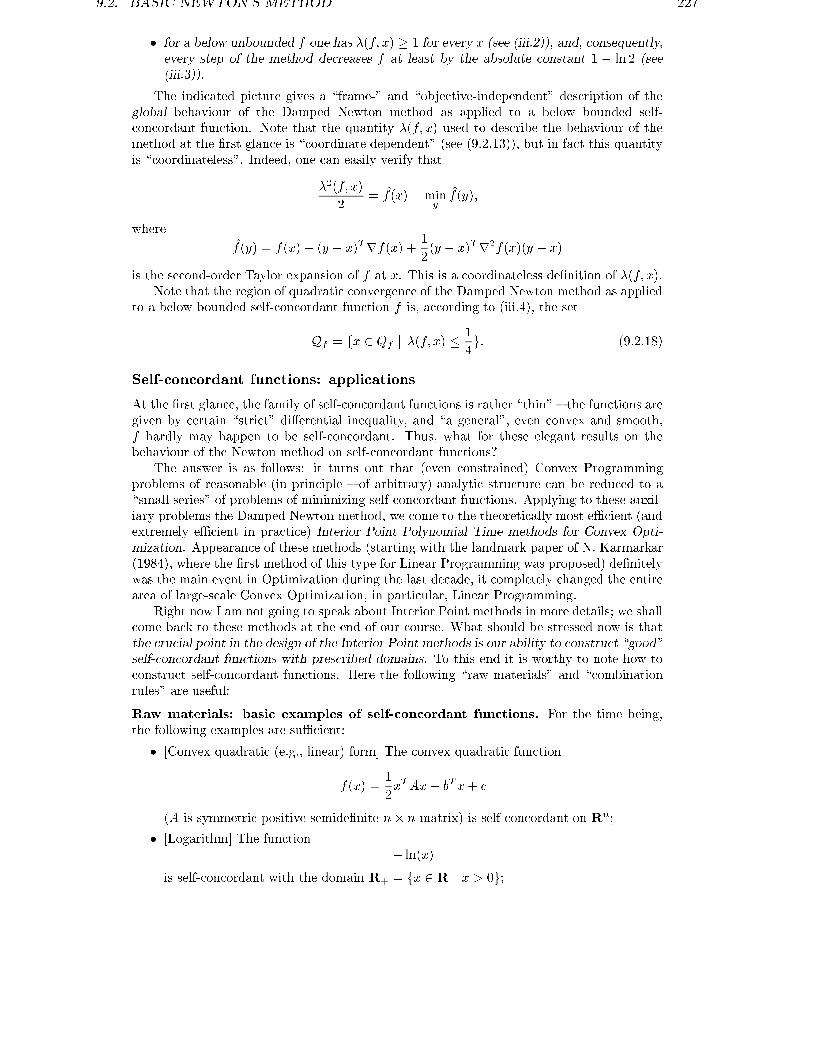
9.2. BASIC NEWTON'S METHOD 227
� for a below unbounded f one has �(f; x) � 1 for every x (see (iii.2)), and, consequently,every step of the method decreases f at least by the absolute constant 1 � ln 2 (see(iii.3)).
The indicated picture gives a \frame-" and \objective-independent" description of theglobal behaviour of the Damped Newton method as applied to a below bounded self-concordant function. Note that the quantity �(f; x) used to describe the behaviour of themethod at the �rst glance is \coordinate dependent" (see (9.2.13)), but in fact this quantityis \coordinateless". Indeed, one can easily verify that
�2(f; x)
2= f(x) �min
yf(y);
where
f(y) = f(x) + (y � x)Trf(x) + 1
2(y � x)Tr2f(x)(y � x)
is the second-order Taylor expansion of f at x. This is a coordinateless de�nition of �(f; x).Note that the region of quadratic convergence of the Damped Newton method as applied
to a below bounded self-concordant function f is, according to (iii.4), the set
Qf = fx 2 Qf j �(f; x) � 1
4g: (9.2.18)
Self-concordant functions: applications
At the �rst glance, the family of self-concordant functions is rather \thin" { the functions aregiven by certain \strict" di�erential inequality, and \a general", even convex and smooth,f hardly may happen to be self-concordant. Thus, what for these elegant results on thebehaviour of the Newton method on self-concordant functions?
The answer is as follows: it turns out that (even constrained) Convex Programmingproblems of reasonable (in principle { of arbitrary) analytic structure can be reduced to a\small series" of problems of minimizing self-concordant functions. Applying to these auxil-iary problems the Damped Newton method, we come to the theoretically most eÆcient (andextremely eÆcient in practice) Interior Point Polynomial Time methods for Convex Opti-mization. Appearance of these methods (starting with the landmark paper of N. Karmarkar(1984), where the �rst method of this type for Linear Programming was proposed) de�nitelywas the main event in Optimization during the last decade, it completely changed the entirearea of large-scale Convex Optimization, in particular, Linear Programming.
Right now I am not going to speak about Interior Point methods in more details; we shallcome back to these methods at the end of our course. What should be stressed now is thatthe crucial point in the design of the Interior Point methods is our ability to construct \good"self-concordant functions with prescribed domains. To this end it is worthy to note how toconstruct self-concordant functions. Here the following \raw materials" and \combinationrules" are useful:
Raw materials: basic examples of self-concordant functions. For the time being,the following examples are suÆcient:
� [Convex quadratic (e.g., linear) form] The convex quadratic function
f(x) =1
2xTAx� bTx+ c
(A is symmetric positive semide�nite n� n matrix) is self-concordant on Rn;
� [Logarithm] The function� ln(x)
is self-concordant with the domain R+ = fx 2 R j x > 0g;

228 LECTURE 9. GRADIENT DESCENT AND NEWTON'S METHOD
� [Extension of the previous example: Logarithmic barrier, linear/quadratic case] Let
Q = fx 2 Rn j �j(x) < 0; j = 1; :::;mgbe a nonempty set in Rn given by m strict convex quadratic (e.g., linear) inequalities.Then the function
f(x) = �mXi=1
ln(��i(x))
is self-concordant with the domain equal to Q.
Combination rules: simple operations with functions preserving self-concordance
� [Linear combination with coeÆcients � 1] Let fi, i = 1; :::m, be self-concordant func-tions with the domains Qfi , let these domains possess a nonempty intersection Q, andlet �i � 1, i = 1; :::;m, be given reals. Then the function
f(x) =mXi=1
�ifi(x)
is self-concordant with the domain equal to Q.
In particular, the sum of a self-concordant function and a convex quadratic function(e.g., a linear one) is self-concordant;
� [AÆne substitution] Let f(x) be self-concordant with the domain Qf � Rn, and letx = A� + b be an aÆne mapping from Rk into Rn with the image intersecting Qf .Then the composite function
g(�) = f(A� + b)
is self-concordant with the domain
Qg = f� j A� + b 2 Qfgbeing the inverse image of Qf under the aÆne mapping in question.
To justify self-concordance of the indicated functions, same as the validity of the combina-tion rules, only minimal e�ort is required; at the same time, these examples and rules givealmost all required to establish excellent global eÆciency estimates for Interior Point meth-ods as applied to Linear Programming and Convex Quadratically Constrained Quadraticprogramming.
After we know examples of self-concordant functions, let us look how our now under-standing of the behaviour of the Newton method on such a function di�ers from the onegiven by Theorem 9.2.1. To this end consider a particular self-concordant function { thelogarithmic barrier
f(x) = � ln(Æ � x1)� ln(Æ + x1)� ln(1� x2)� ln(1 + x2)
for the 2D rectangleD = fx 2 R2 j jx1j < Æ; jx2j < 1g;
in what follows we assume that the rectangle is \wide", i.e., that
Æ >> 1:
This function indeed is self-concordant (see the third of the above \raw material" examples).The minimizer of the function clearly is the origin; the region of quadratic convergence ofthe Damped Newton method is given by
Q = fx 2 D j x21Æ2 + x21
+x22
1 + x22� 1
32g

9.2. BASIC NEWTON'S METHOD 229
(see (9.2.18)). We see that the region of quadratic convergence of the Damped Newtonmethod is large enough { it contains, e.g., 8 times smaller than D concentric to D rectangleD0. Besides this, (9.2.17) says that in order to minimize f to inaccuracy, in terms of theobjective, �, starting with a point x0 2 D, it suÆces to perform no more than
O(1)
�ln
1
k x0 k + ln ln1
�
�steps, where O(1) is an absolute constant and
k x k= maxf jx1jÆ; jx2jg:
Now let us look what Theorem 9.2.1 says. The Hessian r2f(0) of the objective at theminimizer is
H =
�2�2 00 2
�;
and jH�1j = O(Æ2); in, say, 0.5-neighbourhood U of x� = 0 we also have j[r2f(x)]�1j =O(Æ2). The third-order derivatives of f in U are of order of 1. Thus, in the notation fromthe proof of Theorem 9.2.1 we have �1 = O(1) (this is the magnitude of the third orderderivatives of f in U), U 0 = U , r = 0:5 (the radius of the circle U 0 = U) and �2 = O(Æ2)(this is the upper bound on the norm of the inverted Hessian of f in U 0). According to theproof, the region U 00 of quadratic convergence of the Newton method is �-neighbourhood ofx� = 0 with
� = min[r; (2�1�2)�1] = O(�2):
Thus, according to Theorem 9.2.1, the region of quadratic convergence of the method becomesthe smaller the larger is Æ, while the actual behaviour of this region is quite opposite.
In this simple example, the aforementioned drawback of the traditional approach { its\frame-dependence" { is clearly seen. Applying Theorem 9.2.1 to the situation in question,we used extremely bad \frame" { Euclidean structure. If we were clever enough to scale thevariable x1 before applying Theorem 9.2.1 { to divide it by Æ { it would become absolutelyclear that the behaviour of the Newton method is absolutely independent of Æ, and the regionof quadratic convergence of the method is a once for ever �xed \fraction" of the rectangleD.
To extract certain moral from this story about self-concordance, let me note that it is
one of the examples of what is Mathematics and progress in Mathematics: the known from
XVII Century very natural and simple (and seemingly perfectly well understood decades ago)
optimization method gave rise to one of the most advanced and most recent breakthroughs
in Optimization.

230 LECTURE 9. GRADIENT DESCENT AND NEWTON'S METHOD
Assignment # 9 (Lecture 9)
Exercise 9.1 Prove that in the Steepest Descent any two subsequent directions of movementare mutually orthogonal. Derive from this that in the 2D case all directions of movement oneven steps are collinear to each other, and the directions of movement at the odd steps also arecollinear to each other.
Exercise 9.2 Write the code implementing the ArD (or StD , on your choice) and apply it tothe following problems:
� Rosenbrock problem
f(x) = 100(x2 � x21)2 + (1� x1)
2 ! min j x = (x1; x2) 2 R2;
the starting point is x0 = (�1:2; 1).The Rosenbrock problem is a well-known test example: it has a unique critical pointx� = (1; 1) (the global minimizer of f); the level lines of the function are banana-shapedvalleys, and the function is nonconvex and rather badly conditioned.
� Quadratic problem
f�(x) = x21 + �x22 ! min j x = (x1; x2) 2 R2:
Test the following values of �10�1; 10�4; 10�6
and for each of these values test the starting points
(1; 1); (p�; 1); (�; 1):
How long it takes to reduce the initial inaccuracy, in terms of the objective, by factor 0.1?
� Quadratic problem
f(x) =1
2xTAx� bTx; x 2 R4;
with
A =
0BB@0:78 �0:02 �0:12 �0:14�0:02 0:86 �0:04 0:06�0:12 �0:04 0:72 �0:08�0:14 0:06 �0:08 0:74
1CCA ; b =
0BB@0:760:081:120:68
1CCA ; x0 = 0:
Run the method until the norm of the gradient at the current iterate is becomes less than10�6. Is the convergence fast or not?
Those using MatLab can compute the spectrum of A and to compare the theoretical upperbound on convergence rate with the observed one.
� Experiments with Hilbert matrix. Let H(n) be the n� n Hilbert matrix:
(H(n))ij =1
i+ j � 1; i; j = 1; :::; n:
This is a symmetric positive de�nite matrix (since xTH(n)x =R 10 (Pn
i=1 xiti�1)2dt � 0, the
inequality being strict for x 6= 0).
For n = 2; 3; 4; 5 perform the following experiments:

9.2. BASIC NEWTON'S METHOD 231
{ choose somehow n-dimensional nonzero vector x�, e.g., x� = (1; :::; 1)T ;
{ compute b = H(n)x�;
{ Apply your Gradient Descent code to the quadratic function
f(x) =1
2xTH(n)x� bTx;
the starting point being x0 = 0. Note that x� is the unique minimizer of f .
{ Terminate the method when you will get jxN � x�j � 10�4, not allowing it, anyhow,to run more than 10,000 steps.
What will be the results?
Those using MatLab can try to compute the condition number of the Hilbert matrices inquestion.
If you choose to implement ArD , play with the parameters � and � of the method to get thebest possible convergence.

232 LECTURE 9. GRADIENT DESCENT AND NEWTON'S METHOD

Lecture 10
Around the Newton Method
In the previous Lecture we spoke about the Newton method
xt+1 = xt + t+1et; et = �[r2f(xt)]�1rf(xt);
f being the objective to be minimized; from now on we assume the objective to be smoothenough (namely, 3 times continuously di�erentiable) and such that the level set
S = fx j f(x) � f(x0)g;x0 being the starting point of the method in question, is bounded.
We have considered two versions of the method { the basic one, where we all the time usethe unit stepsizes ( t+1 � 1), and version with line search, where t+1 is given by a kind of linesearch applied to the function
�( ) = f(xt + et)
{ to the restriction of the objective on the \search ray" given by the current iterate xt and the\Newton direction" et.
As we remember, the Basic version of the method, being started close enough to a nondegen-erate local minimizer x� of f (one with positive de�nite r2f(x�)) converges to x� quadratically,although may diverge if started far from the optimal set. The Line search version of the methodpossesses global convergence, provided that the objective is convex with nondegenerate Hessian(r2f(x) is positive de�nite for every x). The latter assumption is, however, too restrictive formany applications, and this fact motivates the �rst of our current goals:
A. To modify the Newton method in order to make it globally convergent inde-pendently of the convexity and nondegeneracy assumptions
Of course, the only kind of convergence it makes sense to bother about in the general (non-convex) case is the convergence to the set of critical points of the objective, not to the set ofglobal minimizers of it. And of course the modi�cations we are interested in should preservethe most attractive property of the Basic Newton method { its fast local convergence: if themethod converges to a nondegenerate local minimizer of f , the convergence should, at leastasymptotically, be as fast as for the Basic method.
A. is the �rst of our goals, but not the only one of them. It was mentioned in Lecture 9that from the practical viewpoint a severe shortcoming of the Newton method is the necessity tocompute the Hessians of the objective and to invert these Hessians. This shortcoming motivatesthe second of our goals:
233

234 LECTURE 10. AROUND THE NEWTON METHOD
B. To \imitate" the behaviour of the Newton method in a �rst-order scheme (oneusing only the �rst order derivatives of f and not inverting matrices)
We shall overview three generic modi�cations of the Newton method:
� Modi�ed Newton Methods
� Conjugate Gradient Methods
� Quasi-Newton Methods
The Modi�ed Newton methods take care of the goal A only and ignore the goal B { they still usethe second order derivatives and invert matrices. In contrast to this, both Conjugate Gradientand Quasi-Newton methods are aimed to achieve both goals A and B; the di�erence betweenthese two families is in how they try to achieve these goals.
10.1 Modi�ed Newton methods
10.1.1 Variable Metric Methods
Let us start with developing certain general approach which covers both the Gradient and theNewton methods and allows to understand how to \cure" the Newton method. To outline theidea, let us come back to the Gradient Descent. What in fact we did in this method? Givenprevious iterate x, we used local linear approximation of the objective:
f(y) � f(x) + (y � x)Trf(x) (10.1.1)
and choose, as the next direction of movement, the \most perspective" of descent directions of theright hand side. Now, how we were comparing the directions to choose the \most perspective"one? We took the unit ball
W = fd j dTd � 1gof directions and choose in this ball the direction which minimizes the value
�f(x+ d) � f(x) + dTrf(x)of the approximate objective. This direction, as it is immediately seen, is simply the normalizedanti-gradient direction
�jrf(x)j�1rf(x);and in the Gradient Descent we used it as the current direction of movement, choosing thestepsize in order to achieve \signi�cant" progress in the objective value. Note that instead ofminimizing �f(x+ d) on the ball W , we could minimize the quadratic function
f(d) = dTrf(x) + 1
2dT d
over d 2 Rn; the result will be simply the anti-gradient direction �rf(x). This is not the sameas the above normalized anti-gradient direction, but the di�erence in normalization is absolutelyunimportant for us { in any case we indent to use line search in the generated direction, so thatwhat in fact we are interested in is the search ray fx + d j � 0g, and proportional, withpositive coeÆcient, directions result in the same ray.

10.1. MODIFIED NEWTON METHODS 235
With the outlined interpretation of the Gradient Descent as a method with line search andthe search direction given by minimization of the linearized objective �f(x+ d) over d 2 W , wemay ask ourselves: why we use in this scheme the unit ball W , not something else? E.g., whynot to use an ellipsoid
WA = fd j dTAd � 1g;A being a positive de�nite symmetric matrix?Recall that an ellipsoid in properly chosen coordinates of Rn becomes a ball (the coordinatesare obtained from the standard ones by linear nonsingular transformation). Consequently, amethod of the outlined type with W replaced by WA, i.e., the one where the search direction isgiven by
d = argmind2WA
�f(x+ d) (10.1.2)
has the same \right to exist" as the Gradient Descent. This new \scaled by matrix A GradientDescent" is nothing but the usual Gradient Descent, but associated with the coordinates on Rn
where WA becomes the unit ball. Note that the usual Gradient Descent corresponds to the caseA = I, I being the unit matrix. Now, the initial coordinates are absolutely \occasional" { theyhave nothing in common with the problem we are solving; consequently, we have no reason toprefer these particular coordinates. Moreover, if we were lucky to adjust the coordinates weuse to the \geometry" of the objective (cf. discussion in the previous Lecture), we could get amethod with better convergence than the one of the usual Gradient Descent.
Same as above, the direction given by (10.1.2) is, up to renormalization (the latter, as it wasalready explained, is unimportant { it is \suppressed" by line search), nothing but the directiongiven by the minimization of the quadratic form
fA(d) = dTrf(x) + 1
2dTAd; (10.1.3)
minimizing the right hand side with respect to d (to this end it suÆces to solve the Fermatequation rdfA(d) � rf +Ad = 0), we come to the explicit form of the search direction:
d = �A�1rf(x): (10.1.4)
Note that this direction for sure is a descent direction of f at x, provided that x is not a criticalpoint of f :
rf(x) 6= 0) dTrf(x) = �(rf(x))TA�1rf(x) < 0
(recall that A is symmetric positive de�nite, whence A�1 also is symmetric positive de�nite), sothat we are in a good position to apply to f line search in the direction d.
The summary of our considerations is as follows: choosing a positive de�nite symmetricmatrix A, we can associate with it \A-anti-gradient direction" �A�1rf(x), which is a descentdirection of f at x (provided that rf(x) 6= 0). And we have the same reasons to use thisdirection in order to improve f as those to use the standard anti-gradient direction (given bythe same construction with A = I).
Now we can make one step of generalization more: why should we use at each step of themethod a once for ever �xed matrix A instead of varying this matrix from iteration to iteration?The \geometry" of the objective varies along the trajectory, and it is natural to adjust thematrix A to this varying geometry. Thus, we come to the following generic scheme of a VariableMetric method:

236 LECTURE 10. AROUND THE NEWTON METHOD
Algorithm 10.1.1 [Generic Variable Metric method]Initialization: choose somehow starting point x0 and set t = 0Step t: given previous iterate xt�1,
� compute f(xt�1), rf(xt�1) and, possibly, r2f(xt�1);
� choose somehow positive de�nite symmetric matrix At and compute the At-anti-gradientdirection
dt = �A�1t rf(xt�1)of f at xt�1;
� perform line search from xt�1 in the direction dt, thus getting new iterate
xt = xt�1 + tdt � xt�1 � tA�1t rf(xt�1);
replace t with t+ 1 and loop.
The outlined scheme covers all methods we know so far: to get di�erent versions of the GradientDescent, we should set At � I and should specify the version of the line search to be used.With At = r2f(xt�1), we get, as dt, the Newton direction of f at xt�1, and we come to theNewton method with line search; further specifying the line search by the \programmed" rule t = 1, we get the Basic Newton method. Thus, the Basic Newton method is nothing but theGradient Descent scaled by the Hessian of the objective at the current iterate. Note, anyhow,that the \Newton choice" At = r2f(xt�1) is compatible with the outlined scheme (where At
should be symmetric positive de�nite) only when r2f(xt�1) is positive de�nite1); from theabove discussion we know that if it is not the case, we indeed have no reasons to use the Newtondirection and should somehow modify it to make it descent. Thus, the generic Algorithm 10.1.1covers all we know to the moment and provides us with good idea how to \cure" the Newtonmethod at a \bad" iterate:
at such an iterate, we should replace the actual Hessian At = r2f(xt�1) in the ex-pression �A�1t rf(xt�1) for the Newton direction by its positive de�nite \correction"in order to make the resulting direction descent for the objective.
Thus, we come to the family ofModi�ed Newton methods { those given by the generic Algorithm10.1.1 where we use as At, whenever it is possible, the Hessian r2f(xt�1) of the objective, andwhen it is impossible, choose as At a \positive de�nite correction" of the current Hessian.
Before passing to the Modi�ed Newton methods themselves, we should understand whetherour new scheme indeed achieves our target A { whether it makes the modi�ed method globallyconverging.
10.1.2 Global convergence of a Variable Metric method
We are about to prove that the generic Variable Metric method (Algorithm 10.1.1), under somereasonable restrictions on the matrices At, globally converges to the set of critical points off . The restrictions are very simple: in the generic method, At should be symmetric positivede�nite, and what we need is \uniform" positive de�niteness.
1)the scheme requires also symmetry of At, but here we have no problems: since f is from the very beginningassumed to be three times continuously di�erentiable, its Hessians for sure are symmetric

10.1. MODIFIED NEWTON METHODS 237
Let us say that Algorithm 10.1.1 is uniformly descent with parameters p; P , 0 < p � P <1,if the rules for choosing At in the algorithm ensure that
�min(At) � p; �max(At) � P; t = 1; 2; ::: (10.1.5)
(as always, �min(A)and �max(A) denote the minimal and the maximal eigenvalues of a symmetricmatrix A). Thus, \uniform descentness" simply means that the matrices At never become \toolarge" (their maximal eigenvalues are bounded away from in�nity) and never become \almostdegenerate" (their minimal eigenvalues are bounded away from zero).
Theorem 10.1.1 [Global convergence of uniformly descent Variable Metric method]Let f be twice continuously di�erentiable function, and let x0 be such that the level set
S = fx 2 Rn j f(x) � f(x0)gis bounded. Assume that f is minimized by a uniformly descent Variable Metric method startedat x0, and assume that the line search used in the method is either the exact one-dimensionalline search, or the Armijo-terminated one. Then the trajectory of the method is bounded, theobjective is non-increasing along the trajectory, and all limiting points of the trajectory (whichfor sure exist, since the trajectory is bounded) belong to the set
X�� = fx j rf(x) = 0gof critical points of f .
Proof is similar to the one of Theorem 9.1.1 and is therefore omitted. It is an excellent (non-obligatory!) exercise to restore the proof and to understand what is the role of the \uniformdescentness".
10.1.3 Implementations of the Modi�ed Newton method
Now let us come back to the Newton method. As we remember, our goal is to modify it inorder to assure global convergence (at least the same as the one for the Gradient Descent); and,of course, we would not like to loose the �ne local convergence properties of the method givenby Theorem 9.2.1. We already have an idea how to modify the method: we should use linesearch in a descent direction given by the Variable Metric scheme, where we use, as At, theHessian r2f(xt�1), if the latter matrix is positive de�nite; if it is not the case, we use as At
certain positive de�nite correction of the Hessian. Of course, from both theoretical and numericalreasons, we should modifyr2f(xt�1) not only when it fails to be positive de�nite, but also whenit is \close" to a non-positive-de�nite matrix. Indeed, if we do not modify r2f(xt�1) when it isclose to a non-positive-de�nite matrix, i.e., when the minimal eigenvalue of the Hessian, beingpositive, is small, we are unable to ensure the uniform descent property of the method and,consequently, are unable to ensure global convergence; this is a theoretical reason. The practicalone is that in the outlined case the condition number of the Hessian is large, so that when solvingnumerically the Newton system
r2f(xt�1)e = �rf(xt�1)in order to �nd the Newton direction, we meet with severe numerical problems, and the actuallycomputed direction will be far from the exact one.

238 LECTURE 10. AROUND THE NEWTON METHOD
Thus, our general tactics in the Newton-based implementation of Algorithm 10.1.1 shouldbe as follows: given xt�1, we compute
Ht�1 � r2f(xt�1)
and check whether this matrix is \well positive de�nite"; if it is the case, we use this matrix asAt, otherwise replace Ht�1 with certain \well positive de�nite" correction At of Ht�1. Let uslook at two simplest implementations of the outlined scheme.
Modi�cations based on Spectral Decomposition
Recall that, as it is known from Linear Algebra, any symmetric n�nmatrix A possesses spectraldecomposition
A = UDUT ;
U being an n� n orthogonal matrix:UTU = I;
and D being a diagonal matrix. The diagonal entries of D are exactly the eigenvalues of A,while the columns of U are the associated normalized eigenvectors. In particular, A is positivede�nite if and only if the diagonal entries of D are positive.
In the Modi�ed Newton methods based on spectral decomposition one �nds the indicateddecomposition of the Hessian at every step:
Ht � r2f(xt) = UtDtUTt ; (10.1.6)
and compares the eigenvalues of Ht { i.e., the diagonal entries of Dt { with a once for ever chosen\threshold" Æ > 0. If all the eigenvalues are � Æ, we qualify Ht as \well positive de�nite" anduse it as At+1. If some of the eigenvalues of Ht are < Æ (e.g., are negative), we set
At+1 = Ut �DtUTt ;
where �Dt is the diagonal matrix obtained from D by replacing the diagonal entries smaller thanÆ by Æ. Another way to \correct" Ht is to replace the negative diagonal values in Dt by theirabsolute values (and then to replace by Æ those diagonal entries, if any, which are less than Æ).
Both indicated strategies result in
�min(At) � Æ; t = 1; 2; :::;
and never increase \signi�cantly" the norm of the Hessian:
�max(At) � max [j�max(Ht)j; j�min(Ht)j; Æ] ;
as a result, the associated modi�ed Newton method turns out to be uniformly descent (andthus globally converging), provided that the level set of f associated with the starting point isbounded (so that the Hessians along the trajectory are uniformly bounded). A drawback of theapproach is its relatively large computational cost: to �nd spectral decomposition (10.1.6) tomachine precision, it normally requires between 2n3 and 4n3 arithmetic operations, n being therow size of Ht (i.e., the design dimension of the optimization problem). As we shall see in awhile, this is, in a sense, too much.

10.1. MODIFIED NEWTON METHODS 239
Levenberg-Marquardt Modi�cation
In the Levenberg-Marquardt modi�cation of the Newton method we choose At+1 as the \regu-larization"
At+1 = �tI +Ht (10.1.7)
of the actual Hessian, where the \regularization parameter" �t � 0 is chosen to make the righthand side \well positive de�nite" { to have all its eigenvalues at least the chosen in advancepositive threshold Æ. This is the same as to ensure that At+1 � ÆI 2).
To �nd the desired �t, we �rst check whether the requirement
Ht > ÆI
is satis�ed; if it is the case, we choose �t = 0 and At+1 = Ht, thus getting the pure Newtondirection. Now assume that the inequality Ht � ÆI does not take place. The matrix
A(�) = �I +Ht � ÆI
for sure is positive de�nite when � > 0 is large enough, and in the case in question it is notpositive de�nite for � = 0. Thus, there exists the smallest � = �� � 0 for which A(�) is positivesemide�nite. And what we do in the Levenberg-Marquardt scheme are several steps of thebisection routine to �nd a \tight" upper bound �t for ��. The resulting upper bound is used tocreate At according to (10.1.7).
The essence of the matter is, of course, how we verify whether a given trial value of � is appro-priate, i.e., whether it results in positive semide�nite A(�). It would be absolutely senseless toanswer this question by computing spectral decomposition of A(�) { this computation is exactlywhat we are trying to avoid. Fortunately, in the Linear Algebra there is a much more eÆcientalgorithm for checking positive de�niteness of given symmetric matrix { the Choleski factoriza-tion. This factorization answers the question in approximately n3=6 arithmetic operations, nbeing the size of the matrix we are factorizing. In the Levenberg-Marquardt scheme, we usethis Choleski factorization to govern the Bisection; with this approach, one can check positivede�niteness of A(�) for a given � in about n3=6 arithmetic operations { something from 12 to 24times cheaper than the cost of spectral decomposition. Thus, the Levenberg-Marquardt schemewith 5-10 bisection steps in � (this is suÆcient for \smart" implementation of the scheme) isnumerically less expensive then the scheme based on spectral decomposition.
Choleski Factorization
It is known from Linear Algebra, that a symmetric n�n matrix A is positive de�nite is andonly if it admits factorization
A = LDLT ; (10.1.8)
where
� L is lower-triangular n� n matrix with unit diagonal entries;
� D is diagonal matrix with positive diagonal entries.
2)from now on, for symmetric matrices A;B the inequality A � B means that A�B is positive semide�nite,and A > B means that A�B is positive de�nite. Note that, for a symmetric matrix A, the relation �max(A) � ais equivalent to aI �A � 0, while �min(A) � a is equivalent to A� aI � 0

240 LECTURE 10. AROUND THE NEWTON METHOD
The Choleski Factorization is an algorithm which computes the factors L and D in decom-position (10.1.8), if such a decomposition exists. The algorithm is given by the recurrence
dj = aii �j�1Xs=1
dsl2js; (10.1.9)
lij =1
dj
aij �
j�1Xs=1
dsljslis
!; j � i � n; (10.1.10)
(dj is j-th diagonal entry of D, lij and aij are the entries of L and A, respectively). Theindicated recurrence allows to compute D and L, if they exist, in
Cn = n3
6(1 + o(1))
arithmetic operations (o(1) ! 0; n ! 1), in a numerically stable manner. Note that L iscomputed in the \column by column" fashion: the order of computations is
d1 ! l1;1; ld2;1; :::; ln;1 ! d2 ! ld2;2; ld3;2; :::; ln;2 ! d3 ! ld3;3; ld4;3; :::ln;3 ! :::! dn ! ln;n;
if the right hand side in (10.1.9) turns out to be nonpositive for some j, this indicates thatA is not positive de�nite.
The main advantage of Choleski factorization is not only its ability to check in Cn com-putations whether A is positive de�nite, but also to get, as a byproduct, the factorization(10.1.8) of a positive de�nite A. With this factorization, we can immediately solve the linearsystem
Ax = b;
the solution x to the system can be identi�ed by backsubstitutions { sequential solving, foru, v and x, two triangular and one diagonal systems
Lu = b; Dv = u; LTx = v;
and this computation requires only O(n2) arithmetic operations. The resulting method {
Choleski decomposition with subsequent backsubstitutions (the square root method) { is
thought to be the most eÆcient in the operation count and most numerically stable Lin-
ear Algebra routine for solving linear systems with general-type symmetric positive de�nite
matrices.
10.2 Conjugate Gradient Methods
The family of methods in question address both our goals A and B. The idea of the methodsis as follows. What we are doing in the Newton method can be explained as follows: we believethat our objective f is a quadratic form, and apply direct Linear Algebra tools to �nd, underthis assumption, its minimizer { namely, form and solve with respect to x the linear system
(N) r2f(xt)(x� xt) = �rf(xt);which, for the case of quadratic (and convex) f would give us the minimizer of f . In thenon-quadratic case the resulting x, of course, does not minimize f , and we treat it as our newiterate. The drawbacks of the scheme we are trying to eliminate are that we need second-orderinformation on f to assemble the Newton system (N) and should solve the system in order toget x.

10.2. CONJUGATE GRADIENT METHODS 241
In the Conjugate Gradient scheme we also act as if we were believing that the objective isquadratic, but instead of direct forming and solving (N) we solve the system by an iterativemethod. It turns out that one can choose this method in such a way that it
� (i) does not involve explicitly the matrix of the system; all operations are described interms of the values and the �rst order derivatives of f at subsequent iterates;
� (ii) solves the system exactly in no more than n steps, n being the dimension of x.
Since the iterative method for solving (N) we use is described in terms of the values and thegradients of f , it formally can be applied to an arbitrary smooth objective; and if the objectiveturns out to be convex quadratic form, the method, by (ii), will �nd its minimizer in at mostn steps. In view of the latter property of the method we could expect that if the objective is\nearly quadratic", then n steps of the method, although not resulting in exact minimizer off , give us a much better approximation to the minimizer than the point the method is startedfrom. Choosing this approximation as our new starting point and performing n steps of themethod more, we may hope for new signi�cant reduction in inaccuracy, and so on. Of course, allthese hopes are under the assumption that the objective is \nearly quadratic"; but this indeedwill be eventually our case, if the method will converge, and this latter property will indeed beensured by our construction.
It is clear from the outlined general idea that the \main ingredient" of the scheme is certainiterative method for minimizing convex quadratic forms, and we start with the description ofthis method.
10.2.1 Conjugate Gradient Method: Quadratic Case
Let
f(x) =1
2xTHx� bTx (10.2.1)
be a strongly convex quadratic form, so that H is positive de�nite symmetric matrix. Theunique global minimizer x� of f is the solution to the Fermat equation
rf(x) � Hx� b = 0; (10.2.2)
due to strong convexity, this is the only critical point of f . Thus, it is the same { to minimizea strongly convex quadratic form f on Rn and to solve a linear n� n system of equations
Hx = b (10.2.3)
with symmetric positive de�nite matrix H = r2f .We already spoke about direct Linear Algebra technique for solving (10.2.3) { namely, about
the one based on Choleski decomposition of H. There are other direct Linear Algebra methodsto solve this problem { Gauss elimination, etc. When saying that these methods are \direct", Imean that they work with H \as a whole", and until the matrix is processed, no approximateminimizers of f (i.e., approximate solutions to (10.2.3)) are generated; and after H is processed,we get the exact minimizer (in actual computations { exact up to in uence of rounding errors).In contrast to this, the so called iterative methods for minimizing f (� for solving (10.2.3))generate a sequence of approximate minimizers converging to the exact one. We already knowa method of this type { the Steepest Descent; this method is aimed to minimize nonquadraticfunctions, but one can apply it to a quadratic objective as well.
Now we shall speak about another iterative method for minimizing f { the Conjugate Gra-dient one. I shall start with a non-iterative description of the method.

242 LECTURE 10. AROUND THE NEWTON METHOD
CG: Initial description
Let x0 be the starting point we use when minimizing our quadratic objective. We associate withthis point the Krylov vectors
g0 � Hx0 � b;Hg0;H2g0;H
3g0; :::
and the Krylov subspaces
E0 = f0g; Et = Linfg0;Hg0;H2g0; :::;Ht�1g0g; t = 1; 2; :::
so that Et is the linear span of the �rst t Krylov vectors. It is easily seen that
� The Krylov subspaces grow with t:
E1 � E2 � E3 � :::
� Let k � 0 be the �rst value of t such that the �rst t Krylov vectors are linearly dependent.Then the inclusion
Et � Et+1
is strict for t < k � 1 and is equality for t � k � 1.
Indeed, there is nothing to prove if k = 1 (it is possible if and only if g0 = 0), so thatlet us assume that k > 1 (i.e., that g0 6= 0). When t < k � 1, the dimensions of Et andEt+1 clearly are t, t + 1, respectively, so that the inclusion Et � Et+1 is strict. Now,the vectors g0; Hg0; :::; Hk�2g0 are linearly independent, and if we add to this familythe vector Hk�1g0, we get a linearly dependent set; it follows that the vector we add isa linear combination of the vectors g0; Hg0; :::; Hk�2g0:
Hk�1g0 = �0g0 + �1Hg0 + :::+ �k�2Hk�2g0:
Multiplying relation by H , H2, H3,..., we see that t-th Krylov vector, starting with
t = k, is a linear combination of the previous Krylov vectors, whence (by induction)
it is also a linear combination of the �rst k � 1 of these vectors. Thus, Et = Ek�1
whenever t � k.
Now consider the aÆne sets
Ft = x0 +Et;
and let xt be the minimizer of the quadratic form f on Ft. By de�nition, the trajectory ofthe Conjugate Gradient method as minimizing f , x0 being the starting point, is the sequencex0; x1; :::; xk�1. We are about to prove that
� xk�1 is the global minimizer of f ;
� there exists explicit recurrence which allows to build sequentially the points x1; :::; xk�1.
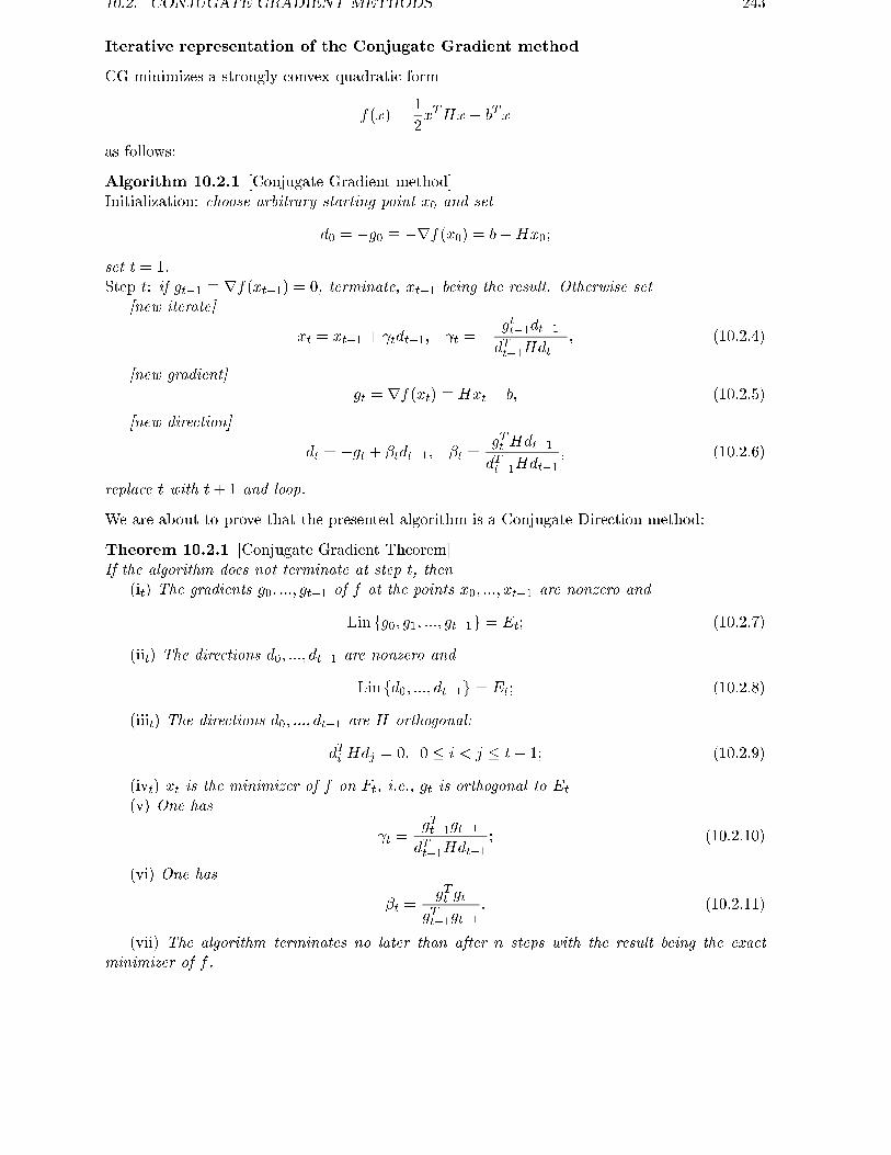
10.2. CONJUGATE GRADIENT METHODS 243
Iterative representation of the Conjugate Gradient method
CG minimizes a strongly convex quadratic form
f(x) =1
2xTHx� bTx
as follows:
Algorithm 10.2.1 [Conjugate Gradient method]Initialization: choose arbitrary starting point x0 and set
d0 = �g0 � �rf(x0) = b�Hx0;
set t = 1.Step t: if gt�1 � rf(xt�1) = 0, terminate, xt�1 being the result. Otherwise set
[new iterate]
xt = xt�1 + tdt�1; t = � gtt�1dt�1dTt�1Hdt�1
; (10.2.4)
[new gradient]gt = rf(xt) � Hxt � b; (10.2.5)
[new direction]
dt = �gt + �tdt�1; �t =gTt Hdt�1dTt�1Hdt�1
; (10.2.6)
replace t with t+ 1 and loop.
We are about to prove that the presented algorithm is a Conjugate Direction method:
Theorem 10.2.1 [Conjugate Gradient Theorem]If the algorithm does not terminate at step t, then
(it) The gradients g0; :::; gt�1 of f at the points x0; :::; xt�1 are nonzero and
Lin fg0; g1; :::; gt�1g = Et; (10.2.7)
(iit) The directions d0; :::; dt�1 are nonzero and
Linfd0; :::; dt�1g = Et; (10.2.8)
(iiit) The directions d0; :::; dt�1 are H-orthogonal:
dTi Hdj = 0; 0 � i < j � t� 1; (10.2.9)
(ivt) xt is the minimizer of f on Ft, i.e., gt is orthogonal to Et
(v) One has
t =gTt�1gt�1dTt�1Hdt�1
; (10.2.10)
(vi) One has
�t =gTt gt
gTt�1gt�1: (10.2.11)
(vii) The algorithm terminates no later than after n steps with the result being the exactminimizer of f .

244 LECTURE 10. AROUND THE NEWTON METHOD
Proof.
10. We �rst prove (i)-(iv) by induction on t.Base t = 1. We should prove that if the algorithm does not terminate at the �rst step
(i.e., if g0 6= 0), then (i1) - (iv1) are valid. The only statement which should be proved is(iv1), and to prove it is the same as to prove that g1 = rf(x1) is orthogonal to E1. This isan immediate corollary of the following
Lemma 10.2.1 Let t be such that gt�1 6= 0. Then gTt dt�1 = 0.
Proof of the Lemma. We have rf(x+ u) = rf(x) +Hu, whence
gTt dt�1 = (gt�1 + tHdt�1)T dt�1 = 0
by de�nition of t, see (10.2.4).Step t 7! t+ 1. Assume that (is) - (ivs) are valid for s � t and that the algorithm does
not terminate at the step t+1, i.e., that gt 6= 0, and let us derive from this assumption (it+1)- (ivt+1).
10. From (ivs), s � t, we know that gs is orthogonal to Es, and from (iis) and (is), thesubspace Es is the linear span of the vectors d0; :::; ds�1, same as it is the linear span of thevectors g0; :::; gs�1, and we conclude that gs is orthogonal to the vectors d0; :::; ds�1:
gTs dl = 0; 0 � l < s � t (10.2.12)
and that the vectors g0; :::; gt are mutually orthogonal:
gTs gl = 0; 0 � l < s � t: (10.2.13)
We have from (10.2.4)
gt = Hxt � b = H(xt�1 + tdt�1)� b = [Hxt�1 � b] + tHdt�1 = gt�1 + tHdt�1:
By (it�1) and (iit�1), both gt�1 and dt�1 belong to Linfg0; Hg0; :::; Ht�1g0g, so that theabove computation demonstrates that gt 2 Linfg0; Hg0; :::; Htg0g, which combined with (it)means that
Linfg0; :::; gtg � Linfg0; Hg0; :::; Htg0g = Et+1:
Since g0; :::; gt are nonzero and mutually orthogonal (see (10.2.13)), the left hand side sub-space in the latter inclusion is of dimension t + 1, while the right hand side subspace is ofdimension at most t + 1; a t + 1-dimensional linear subspace can be enclosed into a linearsubspace of dimension � t+ 1 only if the subspaces are equal, and we come to (it+1).
To prove (iit+1), note that by (10.2.6)
dt = �gt + �tdt�1;
both right hand side vectors are from Et+1 = Linfg0; Hg0; :::; Htg0g (by (iit) and alreadyproved (it+1)), so that dt 2 Linfg0; Hg0; :::; Htg0g; combining this observation with (iit), wecome to
Linfd0; :::; dtg � Linfg0; Hg0; :::; Htg0g: (10.2.14)
Besides this, dt 6= 0 (indeed, gt is nonzero and is orthogonal to dt�1 by (10.2.12)). Now letus prove that dt is H-orthogonal to d0; :::; dt�1. From formula for dt we have
dTt Hds = �gTt Hds + �tdTt�1Hds: (10.2.15)
When s = t�1, the right hand side is 0 by de�nition of �t; and when s < t�1, both terms inthe right hand side are zero. Indeed, the �rst term is zero due to (iit): this relation impliesthat
Hds 2 LinfHg0; H2g0; :::; Hsg0g;

10.2. CONJUGATE GRADIENT METHODS 245
and the right hand side subspace, due to (is+1) (s < t � 1, so that we can use (is+1)!), iscontained in the linear span of the gradients g0; :::; gs+1, and gt is orthogonal to all thesegradients by virtue of (10.2.14) (recall that s < t � 1). The second term in the right handside of (10.2.15) vanishes because of (iiit).
Thus, the right hand side in (10.2.15) is zero for all s < t; in other words, we have proved(iiit+1) { the vectors d0; :::; dt indeed are H-orthogonal. We already know that dt 6= 0; con-sequently, in view of (iit), all d0; :::; dt are nonzero. Since, as we already know, these vectorsare H-orthogonal, they are linearly independent3). Consequently, inclusion in (10.2.14) is infact equality, and we have proved (iit+1).
It remains to prove (ivt+1). We have xt+1 = xt + t+1dt, whence
gt+1 = gt + t+1Hdt:
We should prove that gt+1 is orthogonal to Et+1, i.e., due to already proved (iiit+1), isorthogonal to every di, i � t. Orthogonality of gt+1 and dt is given by Lemma 10.2.1, sothat we should verify that gTt+1di = 0 for i < t. This is immediate:
gTt+1di = gTt di + tdTt Hdi;
the �rst term in the right hand side is zero due to (10.2.12), and the second term is zero dueto already proved (iiit+1).
The inductive step is completed.20. To prove (v), note that if t > 1 then, by (10.2.6),
�gTt�1dt�1 = gTt�1gt�1 � �t�1gTt�1dt�2;
and the second term in the right hand side is 0 due to (10.2.13); thus, �gTt�1dt�1 = gTt�1gt�1for t > 1. For t = 1 this relation also is valid (since, by the initialization rule, d0 =�g0). Substituting equality �gTt�1dt�1 = gTt�1gt�1 into formula for t from (10.2.4), we get(10.2.10).
To prove (vi), note that gTt gt�1 = 0 (see (10.2.14). Besides this, from (10.2.4) we have
Hdt�1 =1
t[gt � gt�1]
(note that t > 0 due to (v) and (it), so that we indeed can rewrite (10.2.4) in the desiredway); taking inner product with gt, we get
gTt Hdt�1 =1
tgTt gt =
dTt�1Hdt�1gTt�1gt�1
gTt gt
(we have used (10.2.10)); substituting the result into (10.2.6), we come to (10.2.11).30. It remains to prove (vii). This is immediate: as we already know, if the method doesnot terminate at step t, i.e., if gt�1 6= 0, then the vectors g0; :::; gt�1 are mutually orthogonalnonzero (and, consequently, linearly independent) vectors which form a basis in Et; sincethere cannot be more than k � 1 � n linearly independent vectors in Et, k being thesmallest t such that the Krylov vectors g0; Hg0; :::; Ht�1g0 are linearly dependent, we seethat the method terminates in no more than k � n steps. And since it is terminated whengt = 0 = rf(xt) = 0, the result of the method indeed is the global minimizer of f .
3)Indeed, we should verify that iftX
i=0
�idi = 0;
then �i = 0, i = 0; :::; t. Multiplying the equality by H and then taking inner product of the result with di, weget
�idTi Hdi = 0
(the terms dTi Hdj with i 6= j are zero due to H-orthogonality of d0; :::; dt), whence �i = 0 (since dTi Hdi > 0 dueto di 6= 0 and to the positive de�niteness of H). Thus, all coeÆcients �i indeed are zeros

246 LECTURE 10. AROUND THE NEWTON METHOD
CG and Three-Diagonal representation of a Symmetric matrix
Assume that we are minimizing (10.2.1) by the Conjugate Gradient algorithm; for the sakeof simplicity, assume also that the method terminates in exactly n steps, so that in courseof its run we obtain n nonzero gradients g0; :::; gn�1. As we know from the proof of theConjugate Gradient Theorem (see (10.2.14)), these gradients are mutually orthogonal, sothat after normalization
fi = jgij�1giof gi we get an orthonormal basis in Rn. How does the matrix H look in this basis? Theanswer is very impressive:
the matrix in the basis ffig is 3-diagonal: fTi Hfj = 0 whenever ji� jj > 1.
The proof is immediate: assume, e.g., that i > j + 1 and let us prove that fTi Hfj =0. As we know from Theorem 10.2.1.(i), fj 2 Linfg0; Hg0; :::; Hjg0g, whence Hfj 2LinfHg0; :::; Hj+1g0g, and the latter subspace is contained in Linfg0; :::; gj+1g (the sameTheorem 10.2.1.(i)). Since, as it was already mentioned, gi is orthogonal to g0; :::; gi�1 andj + 1 < i, we have fTi Hfj = 0, as claimed.
The necessity to �nd an orthonormal basis where a given symmetric matrix becomes3-diagonal occurs in many applications, e.g., when it is necessary to �nd the spectrum (alleigenvalues) of a large and sparse (with close to 0 percentage of nonzero entries) symmetricmatrix. The Conjugate Gradient algorithm is certain \starting point" in developing toolsfor �nding such a basis4).
Rate of convergence of the Conjugate Gradient method
According to Theorem 10.2.1, if CG as applied to (10.2.1) does not terminate during �rst tsteps, xt is the minimizer of f on the aÆne plane
Ft = x0 + Linfd0; :::; dt�1g = x0 +Et;
where, according to (10.2.8),
Et = Linfg0; Hg0; :::; Ht�1g0g; g0 = Hx0 � b: (10.2.16)
Equivalent description of Et is that this is the space comprised of all vectors of the formp(H)g0, p being a polynomial of degree � t� 1:
Et = fp(H)g0 j p(z) =t�1Xi=0
pizig: (10.2.17)
Given these observations, we immediately can establish the following
Proposition 10.2.1 LetE(x) = f(x)�min f
be the residual in terms of the objective associated with quadratic form (10.2.1), and let xtbe t-th iterate of the Conjugate Gradient method (if the method terminates in course of �rstt steps, then, by de�nition, xt is the result of the method, i.e., the exact minimizer of f).Then
E(xt) = minp2Pt�1
1
2(x0 � x�)TH [I �Hp(H)]2(x0 � x�); (10.2.18)
where x0 is the starting point, x� is the exact minimizer of f , I is the unit matrix, and Pkis the family of all polynomials of degree � k.
4)please do not think that the problem in question can be solved by straightforward application of the CG:the in uence of rounding errors makes the actually computed gradients very far from being mutually orthogonal!

10.2. CONJUGATE GRADIENT METHODS 247
Proof is immediate: since f is a quadratic form, we have
f(x) = f(x�)+ (x�x�)Trf(x�)+ 1
2(x�x�)T [r2f ](x�x�) = f(x�)+
1
2(x�x�)TH(x�x�)
(we have taken into account that rf(x�) = 0 and r2f = H), whence
E(x) =1
2(x � x�)H(x� x�): (10.2.19)
Substituting
x = x0 + p(H)g0 = x0 + p(H)(Hx0 � b) = x0 + p(H)H(x0 � x�);
we get x� x� = �[I �Hp(H)](x0 � x�), whence
E(x0 + p(H)g0) =1
2(x0 � x�)TH [1�Hp(H)]2(x� x�):
When p runs through the family Pt�1, the point x0 + p(H)g0, as it already was explained,runs through the aÆne plane Ft = x0 + Et; xt, as we know, is the minimizer of f (and,consequently, E) on this plane, and (10.2.18) follows.
What we are interested in, is the following corollary of Proposition 10.2.1:
Corollary 10.2.1 Let � be the spectrum (the set of distinct eigenvalues) of H, and let xtbe t-th point of the trajectory of CG as applied to f . Then
E(xt) � E(x0) minq2P�t
max�2�
q2(�); (10.2.20)
where P�t is the set of all polynomials q(z) of degree � t equal 1 at z = 0.Besides this,
E(xt) ��1
2jx0 � x�j2
�minq2P�t
max�2�
�q2(�): (10.2.21)
Proof. Let e1; :::; en be an orthonormal basis comprised of eigenvectors of H , and let�1; :::; �n be the corresponding eigenvalues. Let
x0 � x� =nXi=1
siei
be the expansion of x0 � x� in the indicated basis. Then, for any polynomial r,
r(H)(x0 � x�) =nXi=1
r(�i)siei;
applying this identity to the polynomial r(z) = z(1� zp(z))2, p 2 Pt�1, we get
(x0 � x�)2H [1�Hp(H)]2(x0 � x�) =
"nXi=1
siei
#T " nXi=1
�i(1� �ip(�i))2siei
#=
=nXi=1
(1� �ip(�i))2�is
2i : (10.2.22)
The resulting quantity clearly can be bounded from above by
S ��max�2�
(1� �p(�))2� nXi=1
�is2i =
�max�2�
(1� �p(�))2� �(x0 � x�)TH(x0 � x�)
�=

248 LECTURE 10. AROUND THE NEWTON METHOD
[see (10.2.19)].
= 2
�max�2�
(1� �p(�))2�E(x0):
Combining the resulting inequality with (10.2.18), we come to
E(xt) � E(x0) minp2Pt�1
max�2�
(1� �p(�)2:
When p runs through Pt�1, the polynomial q(z) = 1� zp(z) clearly runs through the entireP�t , and (10.2.20) follows.
Relation (10.2.21) is proved similarly; the only di�erence is that instead of boundingfrom above the right hand side of (10.2.22) by the quantity S, we bound the expression by�
max�2�
�(1� �p(�))2� nXi=1
s2i ;
the second factor in the bound being jx0 � x�j2.Corollary 10.2.1 provides us with a lot of information on the rate of convergence of the
Conjugate Gradient method:
� A. Rate of convergence in terms of Condition number It can be proved that for anysegment � = [l; L], 0 < l < L < 1, and for any positive integer s there exists apolynomial qs 2 P�s with
max�2�
q2s(�) � 4
�pQ� 1pQ+ 1
�2s; Q =
L
l:
Combining (10.2.20) and the just indicated result where one should substitute
l = �min(H); L = �max(H);
we get the following non-asymptotical eÆciency estimate for CG as applied to (10.2.1):
E(xN ) � 4
�pQH � 1pQH + 1
�2NE(x0); N = 1; 2; ::: (10.2.23)
where
QH =�max(H)
�min(H)
is the condition number of the matrix H .
We came to a non-asymptotical linear rate of convergence with the convergence ratio�pQH � 1pQH + 1
�2;
for large Qh, this ratio is of the form 1 � O(1)pQH , so that the number of steps
required to improve initial inaccuracy by a given factor � is, independently of thevalue of n, bounded from above by O(1)
pQH ln(1=�). The number of required steps is
proportional to the square root of the condition number of the Hessian, while for theSteepest Descent in the quadratic case similar quantity is proportional to the conditionnumber itself (see Lecture 3); this indeed is a great di�erence!
� B. Rate of convergence in terms of jx0 � x�j It can be proved also that for any L > 0and any integer s > 0 there exists a polynomial rs 2 P�s such that
max0���L
�r2(�) � L
(2s+ 1)2:

10.2. CONJUGATE GRADIENT METHODS 249
Since � for sure is contained in the segment [0; L = jH j], jH j being the norm ofmatrix H , we can use just indicated result and (10.2.21) to get non-asymptotical (andindependent on the condition number of H) sublinear eÆciency estimate
E(xN ) � jH jjx0 � x�j22
1
(2N + 1)2; N = 1; 2; ::: (10.2.24)
This result resembles sublinear global eÆciency estimate for Gradient Descent as ap-plied to a convex C1;1 function (Lecture 9, Proposition 9.1.2); note that a convexquadratic form (10.2.1) indeed is a C1;1 function with Lipschitz constant of gradientequal to jH j. As compared to the indicated result about Gradient Descent, where theconvergence was with the rate O(1=N), the convergence given by (10.2.24) is twicebetter in order { O(1=N2).
� C. Rate of convergence in terms of the spectrum of H The above results establishedrate of convergence of CG in terms of bounds { both lower and upper or only the upperone { on the eigenvalues of H . If we take into account details of the distribution of theeigenvalues, more detailed information on convergence rate can be obtained. Let
�max(H) � �1 > �2 > ::: > �m � �min(H)
be distinct eigenvalues of H written down in descent order. For every k � s let
�k(z) =kYi=1
(1� z=�i) 2 P�k ;
and let qs;k 2 P�s be the polynomial such that
max�min(H)����k+1
q2s;k(�) � 4
"pQk;H � 1pQk;H + 1
#2s; Qk;H =
�k+1�min(H)
(existence of such a polynomial is mentioned in item A). It is clear that
max�2�
[�k(�)qs;k(�)]2 � 4
"pQk;H � 1pQk;H + 1
#2s
(indeed, �k vanishes on the spectrum of H to the right of �k+1 and is in absolute value� 1 between zero and �k+1, while qs;k satis�es the required bound to the left of �k+1in �). Besides this, �kqs;k 2 P�k+s. Consequently, by (10.2.20)
E(xN ) � 4 min1�s�N
8<:"p
QN�s;H � 1pQN�s;H + 1
#2s9=;E(x0)
{ this is an extension of the estimate (10.2.23) (this latter estimate corresponds to thecase when we eliminate the outer min and set s = N in the inner brackets, whichresults in Q0;H = QH). We see also that if N � m, m being the number of distincteigenvalues in H , then E(xN ) = 0 (set q = �m in (10.2.20)); thus, in fact
CG �nds the exact minimizer of f in at most as many steps as many distinct eigenvaluesare there in matrix H .
Taking into account the details of the spectrum of H , one can strengthen the estimateof item B as well.

250 LECTURE 10. AROUND THE NEWTON METHOD
Conjugate Gradient algorithm for quadratic minimization: advantagesand disadvantages
Let us summarize our knowledge on the CG algorithm for (strongly convex) quadratic min-imization, or, which is the same, for solving linear systems
Hx = b
with positive de�nite symmetric matrix H .First of all, note that the method is simple in implementation { as simple as the Gradient
Descent: a step of the method requires not more than 2 multiplications of vectors by ma-trix A. Indeed, literally reproducing formulae (10.2.4) - (10.2.6), you need 2 matrix-vectormultiplications:
dt�1 ! Hdt�1 to �nd t,and
xt ! Hxt to �nd gt.In fact only the �rst of these matrix-vector multiplication is necessary, since gt can becomputed recursively:
gt = gt�1 + tHdt�1 [since gt � gt�1 = H(xt � xt�1) = tHdt�1]:
Note that all remaining actions at a step are simple { taking inner products and linearcombinations of vectors, and all these actions together cost O(n) arithmetic operations.Thus, the arithmetic cost of a step in CG (same as that one for Steepest Descent) is
O(n) + [cost of a single matrix-vector multiplication d! Hd]:
This is a very important fact. It demonstrates that sparsity of H { relatively small numberN (N << n2) of nonzero entries { can be immediately utilized by CG. Indeed, in the\dense" case matrix-vector multiplication costs 2n2 multiplications and additions, and thisis the principal term in the arithmetic cost of a step of the method; in the sparse case thisprincipal term reduces to 2N << 2n2.
Large-scale linear systems of equations typically have matrices H which either are ex-tremely sparse (something 0:01% � 1% of nonzero entries), or are not sparse themselves,but are products of two sparse matrices (\implicit sparsity", e.g., the least square matricesarising in Tomography); in this latter case matrix-vector multiplications are as cheap as ifH itself were sparse. If the size of the matrix is large enough (tens of thousands; in Tomog-raphy people deal with sizes of order of 105 - 106) and no sparsity { explicit or \implicit" {is present, then, typically, there are no ways to solve the system. Now, if the matrix of thesystem is sparse and the pattern of the nonzero entries is good enough, one can solve thesystem by a kind of Choleski decomposition or Gauss elimination, both the methods beingmodi�ed in order to work with sparse data and not to destroy sparsity in course of theirwork. If the matrix is large and sparsity is not \well-structured" or is \implicit", the directmethods of Linear Algebra are unable to solve the system, and all we can do is to use aniterative method, like Steepest Descent or CG. Here we exploit the main advantage of aniterative method based on matrix-vector multiplications { cheap step and modest memoryrequirements.
The indicated advantages of iterative methods are shared by both Steepest Descent andConjugate Gradient. But there is an important argument in favour of CG { its better rateof convergence. In fact, the Conjugate Gradient algorithm possesses the best, in certainexact sense, rate of convergence an iterative method (i.e., the one based on matrix-vectormultiplications) may have.
These are the main advantages of the CG { simplicity and theoretical optimality amongthe iterative methods for quadratic minimization. And the main disadvantage of the methodis its sensitivity to the condition number of the matrix of the system { although less than the

10.2. CONJUGATE GRADIENT METHODS 251
one for Steepest Descent (see item A in the discussion above), but still rather unpleasant.Theoretically, all bad we could expect of an ill-conditioned H is that the convergence of CGwill be slow, but after n steps (as always, n is the size of H) the method should magicallybring us the exact solution. The in uence of rounding errors makes this attractive pictureabsolutely unrealistic. Even with moderate condition number of H , the method will not �ndexact solution in n steps, but will come rather close to it; and with large condition number,the n-th approximate solution can be even worse than the initial one. Therefore when people,by some reasons, are interested to solve a moderate-size linear system by CG, they allow themethod to run 2n, 4n or something like steps (I am saying about \moderate size" systems,since for large-scale ones 2n or 4n steps of CG simply cannot be carried out in reasonabletime).
The conclusion here should be as follows: if you are solving a linear system with sym-
metric positive de�nite matrix and the size of the system is such that direct Linear Algebra
methods { like Choleski decomposition { can be run in reasonable time, it is better to use
these direct methods, since they are much more numerically stable and less sensitive to the
conditioning of the system than the iterative methods. It makes sense to solve the system
by CG only when the direct methods cannot be used, and in this case your chances to solve
the problem heavily depend on whether you can exploit explicit or implicit sparsity of the
matrix in question and especially on how well-conditioned is the matrix.
10.2.2 Extensions to non-quadratic problems
To the moment we in fact dealt not with unconstrained minimization, but with the LinearAlgebra problem of solving a linear system with positive de�nite symmetric matrix. All thiswork in fact was aimed to develop extensions of the Conjugate Gradient algorithm on thenonquadratic case, and it is time now to come to these extensions.
The idea behind the extensions in question is as follows: the Conjugate Gradient Algorithmin its basic version 10.2.1:
(A): g0 = rf(x0); d0 = �g0;(B): xt = xt�1 + tdt�1; t = � gtt�1dt�1
dTt�1Hdt�1;
(C): gt = rf(xt) :(D): dt = �gt + �tdt�1; �t =
gTt Hdt�1dTt�1Hdt�1
;
\almost ignores" the quadratic nature of f : the matrix H is involved only in the formulae forscalars t (the stepsize) and �t (the coeÆcient in the updating formulae for the search directions).If we were able to eliminate the presence of H completely and to describe the process in termsof f and rf only, we would get a recurrence CG� which, formally, could be applied to anarbitrary objective f , and in the case of strongly convex quadratic objective would becomeour basic method CG. This latter method solves quadratic problem exactly in n steps; sinceclose to a nondegenerate local minimizer x� a general smooth objective f is very similar to astrongly convex quadratic one fq, we could hope that CG� applied to f and started close to x�
would \signi�cantly" reduce inaccuracy in n steps. Now we could again apply to f n steps ofthe same routine CG�, but with the starting point given by the �rst n steps, again hopefullysigni�cantly reducing inaccuracy, and so on. If, besides this, we were clever enough to ensureglobal convergence of the indicated \cyclic" routine, we would get a globally converging methodwith good asymptotical behaviour.
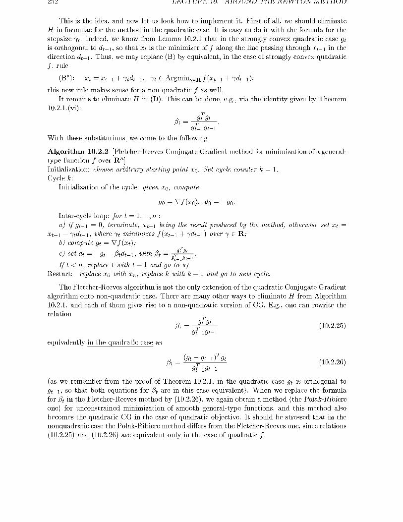
252 LECTURE 10. AROUND THE NEWTON METHOD
This is the idea, and now let us look how to implement it. First of all, we should eliminateH in formulae for the method in the quadratic case. It is easy to do it with the formula for thestepsize t. Indeed, we know from Lemma 10.2.1 that in the strongly convex quadratic case gtis orthogonal to dt�1, so that xt is the minimizer of f along the line passing through xt�1 in thedirection dt�1. Thus, we may replace (B) by equivalent, in the case of strongly convex quadraticf , rule
(B�): xt = xt�1 + tdt�1; t 2 Argmin 2R f(xt�1 + dt�1);
this new rule makes sense for a non-quadratic f as well.It remains to eliminate H in (D). This can be done, e.g., via the identity given by Theorem
10.2.1.(vi):
�t =gTt gt
gTt�1gt�1:
With these substitutions, we come to the following
Algorithm 10.2.2 [Fletcher-Reeves Conjugate Gradient method for minimization of a general-type function f over Rn]Initialization: choose arbitrary starting point x0. Set cycle counter k = 1.Cycle k:
Initialization of the cycle: given x0, compute
g0 = rf(x0); d0 = �g0;Inter-cycle loop: for t = 1; :::; n :a) if gt�1 = 0, terminate, xt�1 being the result produced by the method, otherwise set xt =
xt�1 + tdt�1, where t minimizes f(xt�1 + dt�1) over 2 R;b) compute gt = rf(xt);c) set dt = �gt + �tdt�1, with �t =
gTt gtgTt�1gt�1
.
If t < n, replace t with t+ 1 and go to a)Restart: replace x0 with xn, replace k with k + 1 and go to new cycle.
The Fletcher-Reeves algorithm is not the only extension of the quadratic Conjugate Gradientalgorithm onto non-quadratic case. There are many other ways to eliminate H from Algorithm10.2.1, and each of them gives rise to a non-quadratic version of CG. E.g., one can rewrite therelation
�t =gTt gt
gTt�1gt�1(10.2.25)
equivalently in the quadratic case as
�t =(gt � gt�1)T gtgTt�1gt�1
(10.2.26)
(as we remember from the proof of Theorem 10.2.1, in the quadratic case gt is orthogonal togt�1, so that both equations for �t are in this case equivalent). When we replace the formulafor �t in the Fletcher-Reeves method by (10.2.26), we again obtain a method (the Polak-Ribiereone) for unconstrained minimization of smooth general-type functions, and this method alsobecomes the quadratic CG in the case of quadratic objective. It should be stressed that in thenonquadratic case the Polak-Ribiere method di�ers from the Fletcher-Reeves one, since relations(10.2.25) and (10.2.26) are equivalent only in the case of quadratic f .

10.2. CONJUGATE GRADIENT METHODS 253
10.2.3 Global and local convergence of Conjugate Gradient methods in non-quadratic case
Proposition 10.2.2 [Global convergence of the Fletcher-Reeves and the Polak-Ribiere meth-ods]Let a continuously di�erentiable function f : Rn ! R be minimized by the Fletcher-Reeves orthe Polak-Ribiere versions of the Conjugate Gradient method. Assume that the starting point x0of the �rst cycle is such that the level set
S = fx j f(x) � f(x0)g
is bounded, and let xk be the starting point of cycle k (i.e., the result of the previous cycle).Then the sequence fxkg is bounded, and all limiting points of this sequence are critical points off .
The proof, basically, repeats the one for the Steepest Descent, and I shall only sketch it.The �rst observation is that the objective never increases along the trajectory, since all stepsof the method are based on precise line search. In particular, the trajectory never leaves thecompact set S.
Now, the crucial observation is that the �rst step of cycle k is the usual Steepest Descentstep from xk and therefore it \signi�cantly" decreases f , provided that the gradient of f atxk is not very small 5). Since the subsequent inter-cycle steps do not increase the objective,we conclude that the sum of progresses in the objective values at the Steepest Descent stepsstarting the cycles is bounded from above (by the initial residual in terms of the objective).Consequently, these progresses tend to zero as k ! 1, and due to the aforementionedrelation
small progress in the objective at a Steepest Descent step from xk�1 )
) small jrf(xk�1)jwe conclude that rf(xk) ! 0, k ! 1. Thus, any limiting point of the sequence fxkg is acritical point of f .
The actual justi�cation of non-quadratic extensions of the Conjugate Gradient method is thefollowing proposition which says that the property \�nite n-step convergence" of the methodin the quadratic case transforms into the property of \n-step quadratic convergence" in thenonquadratic one:
Proposition 10.2.3 [Asymptotical \n-step quadratic" convergence of the Fletcher-Reeves andPolak-Ribiere methods in nonquadratic nondegenerate case]Let f : Rn ! R be three times continuously di�erentiable function, and let x� be a nondegeneratelocal minimizer of f , so that rf(x�) = 0 and r2f(x�) is positive de�nite. Assume that f isminimized by the Fletcher-Reeves or Polak-Ribiere versions of the Conjugate Gradient algorithm,
5)all is going on within a compact set S where f is continuously di�erentiable; therefore for x 2 S we have
f(x+ h) � f(x) + hTrf(x) + �(jhj)jhj; 8(h; jhj � 1);
with independent of x 2 S reminder �(s)! 0, s! 0. Consequently, properly chosen step from a point x 2 S inthe anti-gradient direction indeed decreases f at least by (jrf(x)j), with some positive on the ray s > 0 andnondecreasing on the ray function (s)
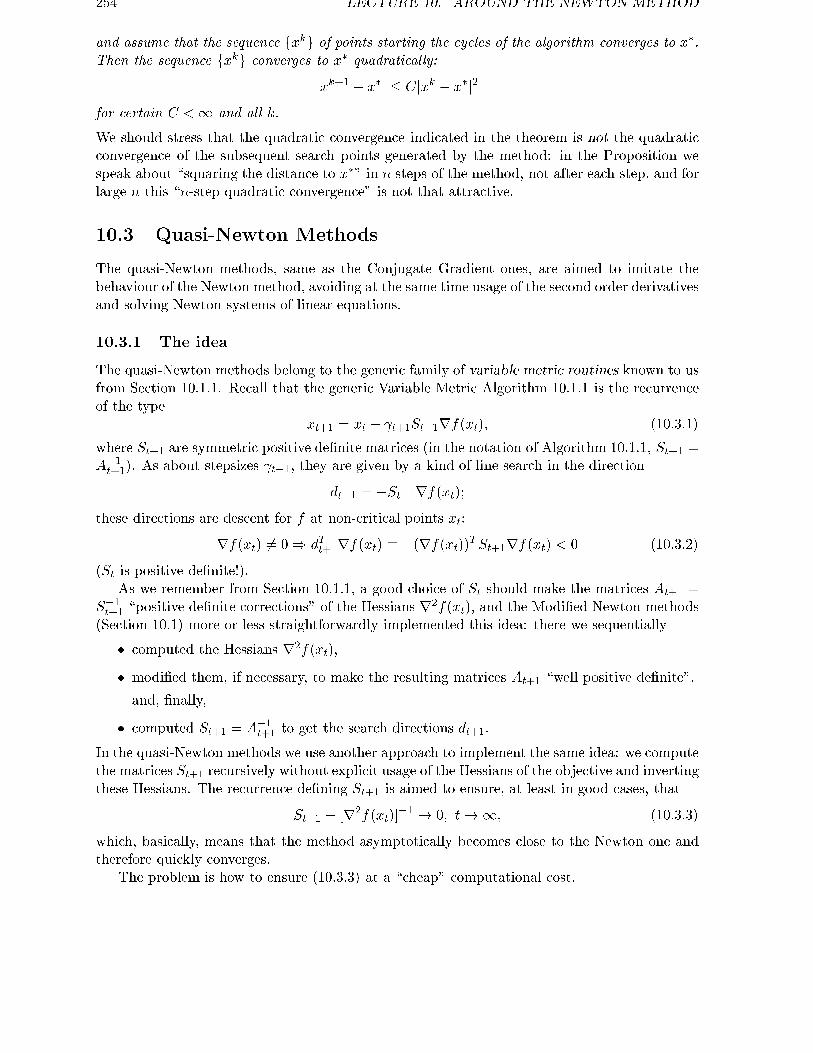
254 LECTURE 10. AROUND THE NEWTON METHOD
and assume that the sequence fxkg of points starting the cycles of the algorithm converges to x�.Then the sequence fxkg converges to x� quadratically:
jxk+1 � x�j � Cjxk � x�j2for certain C <1 and all k.
We should stress that the quadratic convergence indicated in the theorem is not the quadraticconvergence of the subsequent search points generated by the method: in the Proposition wespeak about \squaring the distance to x�" in n steps of the method, not after each step, and forlarge n this \n-step quadratic convergence" is not that attractive.
10.3 Quasi-Newton Methods
The quasi-Newton methods, same as the Conjugate Gradient ones, are aimed to imitate thebehaviour of the Newton method, avoiding at the same time usage of the second order derivativesand solving Newton systems of linear equations.
10.3.1 The idea
The quasi-Newton methods belong to the generic family of variable metric routines known to usfrom Section 10.1.1. Recall that the generic Variable Metric Algorithm 10.1.1 is the recurrenceof the type
xt+1 = xt � t+1St+1rf(xt); (10.3.1)
where St+1 are symmetric positive de�nite matrices (in the notation of Algorithm 10.1.1, St+1 =A�1t+1). As about stepsizes t+1, they are given by a kind of line search in the direction
dt+1 = �St+1rf(xt);these directions are descent for f at non-critical points xt:
rf(xt) 6= 0) dTt+1rf(xt) � �(rf(xt))TSt+1rf(xt) < 0 (10.3.2)
(St is positive de�nite!).As we remember from Section 10.1.1, a good choice of St should make the matrices At+1 =
S�1t+1 \positive de�nite corrections" of the Hessians r2f(xt), and the Modi�ed Newton methods(Section 10.1) more or less straightforwardly implemented this idea: there we sequentially
� computed the Hessians r2f(xt),
� modi�ed them, if necessary, to make the resulting matrices At+1 \well positive de�nite",
and, �nally,
� computed St+1 = A�1t+1 to get the search directions dt+1.
In the quasi-Newton methods we use another approach to implement the same idea: we computethe matrices St+1 recursively without explicit usage of the Hessians of the objective and invertingthese Hessians. The recurrence de�ning St+1 is aimed to ensure, at least in good cases, that
St+1 � [r2f(xt)]�1 ! 0; t!1; (10.3.3)
which, basically, means that the method asymptotically becomes close to the Newton one andtherefore quickly converges.
The problem is how to ensure (10.3.3) at a \cheap" computational cost.

10.3. QUASI-NEWTON METHODS 255
10.3.2 The Generic Quasi-Newton Scheme
The idea behind the below policies for ensuring (10.3.3) is very simple. We intend to generateSt recursively. Namely, assume that at the step t (when updating xt�1 into xt) we used certainapproximation St of the matrix
[r2f(xt�1)]�1;
so that xt was obtained from xt�1 by certain step in the direction
�Stgt�1; gs � rf(xs):
Thus,pt � xt � xt�1 � � tStgt�1; (10.3.4)
t being the stepsize given by linesearch. The �rst-order information on f at the points xt andxt�1 allows us to de�ne the vectors
qt � gt � gt�1: (10.3.5)
If the step pt is small in norm (as it should be the case at the �nal stage) and f is twicecontinuously di�erentiable (which we assume from now on), then
qt � gt � gt�1 � rf(xt)�rf(xt�1) � [r2f(xt�1)](xt � xt�1) � [r2f(xt�1)]pt; (10.3.6)
of course, if f is quadratic, � is simply an equality, independently of whether pt is small or not.Thus, after the step t we have enriched our information on the Hessian: now we have not
only the previous approximation St to [r2f(xt�1)]�1, but also some approximation (namely,qt) to the vector [r2f(xt�1)]pt. We can use this additional information to update the previousapproximation to the inverse Hessian. The simplest and the most natural idea is to impose onSt+1 the following condition (which is an equality version of the approximate equality (10.3.6)):
St+1qt = pt:
This relation, of course, can be satis�ed by in�nitely many updatings St 7! St+1, and thereare di�erent \natural" ways to specify this updating. When the policy of the updatings is�xed, we get a particular version of the generic Variable Metric algorithm, up to the freedomin the linesearch tactics. We shall always assume in what follows that this latter issue { whichlinesearch to use { is resolved in favour of the exact linesearch. Thus, the generic algorithm weare going to consider is as follows:
Algorithm 10.3.1 [Generic Quasi-Newton method]Initialization: choose somehow starting point x0, the initial positive de�nite symmetric matrixS1, compute g0 = rf(x0) and set t = 0.Step t: given xt�1, gt�1 = rf(xt�1) 6= 0 and St, check whether gt�1 = 0. If it is the case,terminate (xt�1 is a critical point of f), otherwise
� setdt = �Stgt�1;
� perform exact line search from xt�1 in the direction dt, thus getting new iterate
xt = xt�1 + tdt;

256 LECTURE 10. AROUND THE NEWTON METHOD
� compute gt = rf(xt) and set
pt = xt � xt�1; qt = gt � gt�1;
� (U): update St into positive de�nite symmetric matrix St+1, maintaining the relation
St+1qt = pt; (10.3.7)
replace t with t+ 1 and loop.
When specifying the only \degree of freedom" in the presented generic algorithm, i.e., the rulesfor (U), our targets are at least the following:
� (A) the matrices St should be symmetric positive de�nite;
� (B) in the case of strongly convex quadratic f the matrices St should converge (ideally {in �nite number of steps) to the inverse Hessian [r2f ]�1.
The �rst requirement is the standard requirement for Variable Metric algorithms; it was moti-vated in Section 10.1.1. The second requirement comes from our �nal goal { to ensure, at leastin good cases (when the trajectory converges to a nondegenerate local minimizer of f), thatSt+1 � [r2f(xt)]�1 ! 0; t ! 1; as we remember, this property underlies fast { superlinear {asymptotical convergence of the algorithm.
Implementing (U) in a way which ensures the indicated properties and incorporating, inaddition, certain policies which make the algorithm globally converging (e.g., restarts, which wealready have used in non-quadratic extensions of the Conjugate Gradient method), we will cometo globally converging methods with nice, in good cases, asymptotical convergence properties.
In the rest of the Lecture we focus on two frequently used forms of updating (U)
10.3.3 Implementations
Davidon-Fletcher-Powell method
In this method, (U) is given by
St+1 = St +1
pTt qtptp
Tt �
1
qTt StqtStqtq
Tt St: (10.3.8)
We are about to demonstrate that (10.3.8) is well-de�ned, results in positive de�nite St+1 andmaintains (10.3.7).
Proposition 10.3.1 Let R be a positive de�nite symmetric matrix, and let p and q be twovectors such that
pT q > 0: (10.3.9)
Then the matrix
R0 = R+1
pT qppT � 1
qTRqRqqTR (10.3.10)
is symmetric positive de�nite and satis�es the relation
R0q = p: (10.3.11)

10.3. QUASI-NEWTON METHODS 257
Proof. 10. Let us prove that R0 satis�es (10.3.11). Indeed, we have
R0q = Rq +1
pT q(pT q)p� 1
qTRq(qTRq)Rq = Rq + p�Rq = p:
20. It remains to verify that R0 is positive de�nite. Let x be an arbitrary nonzero vector;we should prove that xTR0x > 0. Indeed,
xTR0x = xTRx+(xT p)2
pT q� (xTRq)2
qTRq;
setting a = R1=2x; b = R1=2q, we can rewrite the relation as
xTR0x =(aT a)(bT b)� (aT b)2
bT b+(xT p)2
pT q:
Since, by assumption, pT q > 0, the second fraction is nonnegative. The �rst one also is
nonnegative by Cauchy's inequality. Thus, xTR0x � 0, while we need to prove that this
quantity is positive. To this end it suÆces to verify that both numerators in the right hand
side of the latter relation cannot vanish simultaneously. Indeed, the �rst numerator can
vanish only if a is proportional to b (this is said by Cauchy's inequality: it becomes equality
only when the vectors in question are proportional). If a is proportional to b, then x is
proportional to q (see the origin of a and b). But if x = sq for some nonzero (x is nonzero!)
s, then the second numerator is s2(qT p)2, and we know that qT p is positive.
Now we can prove that (10.3.8) indeed can be used as (U):
Proposition 10.3.2 Let at a step t of Algorithm 10.3.1 with (U) given by (10.3.8) the matrixSt be positive de�nite and gt�1 = rf(xt�1) 6= 0 (so that xt�1 is not a critical point of f , and thestep t indeed should be performed). Then St+1 is well-de�ned, is positive de�nite and satis�es(10.3.7).
Proof. It suÆces to verify that qTt pt > 0; then we would be able to get all we need fromProposition 10.3.1 (applied with R = St; q = qt; p = pt).
Since gt�1 6= 0 and St is positive de�nite, the direction dt = �Stgt�1 is a descent directionof f at xt�1 (see (10.3.2)). Consequently, the exact linesearch results in a nonzero stepsize,and pt = xt � xt�1 = tdt 6= 0. We have
qTt pt = t(gt � gt�1)T dt =
[since xt is a minimizer of f on the ray fxt�1 + dt j > 0g and therefore gt is orthogonalto the direction dt of the ray]
= � tgTt�1dt = tgTt�1Stgt�1 > 0
(St is positive de�nite).
It can be proved that the Davidon-Fletcher-Powell method, as applied to a strongly convexquadratic form, �nds exact solution in no more than n steps. n being the dimension of thedesign vector. Moreover the trajectory generated by the method initialized with S1 = I isexactly the one of the Conjugate Gradient method, so that the DFP (Davidon-Fletcher-Powell)method with the indicated initialization is a Conjugate Gradient method { in the quadratic caseit becomes the standard Conjugate Gradient.

258 LECTURE 10. AROUND THE NEWTON METHOD
The Broyden family
The DFP version of (U) is certain rank 2 formula { the updated matrix St+1 di�ers from St bya matrix of rank 2. The Broyden family of quasi-Newton methods is based on another rank 2updating formula { the Broyden-Fletcher-Goldfarb-Shanno one.
The formula is as follows (those interested in its derivation are referred to Appendix to thelecture):
(I) SBFGSt+1 = St +1+qTt Stqt(pTt qt)
2 ptpTt � 1
pTt qt
hptqTt St + StqtpTt
i(we write BFGS to indicate that this is the Broyden-Fletcher-Goldfarb-Shanno updating). It canbe proved (see Proposition 10.3.3 in Appendix) that (I) is a correct version of (U): independentlyof what is positive de�nite symmetric St, (I) results in positive de�nite symmetric St+1 satisfyingthe relation
(*) St+1qt = pt;
exactly as the Davidon-Fletcher-Powell updating
(II) SDFPt+1 = St +1
qTt ptptpTt � 1
qTt StqtStqtqTt St:
Now we have two updating formulae { (I) and (II); they transform a positive de�nite matrix Stinto positive de�nite matrices SBFGSt+1 and SDFPt+1 , respectively, satisfying (*). Since (*) is linearin St+1, any convex combination of the resulting matrices also satis�es (*). Thus, we come tothe Broyden implementation of (U) given by
S�t+1 = (1� �)SDFPt+1 + �SBFGSt+1 ; (10.3.12)
here � 2 [0; 1] is the parameter specifying the updating. Note that the particular case of � = 0corresponds to the Davidon-Fletcher-Powell method.
One can verify by a direct computation that
S�t+1 = SDFPt+1 + �vt+1vTt+1; vt+1 = (qTt Stqt)
1=2
"1
pTt qtpt � 1
qTt StqtStqt
#: (10.3.13)
From the considerations which led us to (10.3.12), we get the following
Corollary 10.3.1 A Broyden method, i.e., Algorithm 10.3.1 with (U) given by (10.3.12), � 2[0; 1] being the parameter of the method (which may vary from iteration to iteration), is a quasi-Newton method: it maintains symmetry and positive de�niteness of the matrices St and ensures(10.3.7).
It can be proved that, as applied to a strongly convex quadratic form f , the Broyden methodminimizes the form exactly in no more than n steps, n being the dimension of the design vector,and if S0 is proportional to the unit matrix, then the trajectory of the method on f is exactlythe one of the Conjugate Gradient method.
There is the following remarkable fact:
all Broyden methods, independently of the choice of the parameter �, being started from thesame pair (x0; S1), equipped with the same exact line search and being applied to the sameproblem, generate the same sequence of iterates (although not the same sequence of matricesHt!).
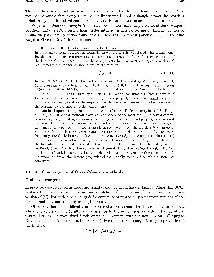
10.3. QUASI-NEWTON METHODS 259
Thus, in the case of exact line search all methods from the Broyden family are the same. Themethods became di�erent only when inexact line search is used; although inexact line search isforbidden by our theoretical considerations, it is always the case in actual computations.
Broyden methods are thought to be the most eÆcient practically versions of the ConjugateGradient and quasi-Newton methods. After intensive numerical testing of di�erent policies oftuning the parameter �, it was found that the best is the simplest policy � � 1, i.e., the pureBroyden-Fletcher-Goldfarb-Shanno method.
Remark 10.3.1 Practical versions of the Broyden methods.In practical versions of Broyden methods, exact line search is replaced with inexact one.Besides the standard requirements of \signi�cant decrease" of the objective in course ofthe line search (like those given by the Armijo test), here we meet with speci�c additionalrequirement: the line search should ensure the relation
pTt qt > 0: (10.3.14)
In view of Proposition 10.3.1 this relation ensures that the updating formulae (I) and (II)(and, consequently, the �nal formula (10.3.12) with � 2 [0; 1]) maintain positive de�nitenessof St's and relation (10.3.7), i.e., the properties crucial for the quasi-Newton methods.
Relation (10.3.14) is ensured by the exact line search (we know this from the proof ofProposition 10.3.2), but of course not only by it: the property is given by a strict inequalityand therefore, being valid for the stepsize given by the exact line search, is for sure valid ifthe stepsize is close enough to the \exact" one.
Another important implementation issue is as follows. Under assumption (10.3.14), up-dating (10.3.12) should maintain positive de�niteness of the matrices St. In actual compu-tations, anyhow, rounding errors may eventually destroy this crucial property, and when ithappens, the method may become behave itself crazy. To overcome this diÆculty, in goodimplementations people store and update from step to step not the matrices St themselves,but their Choleski factors: lower-triangular matrices Ct such that St = CtCT
t , or, morefrequently, the Choleski factors C 0t of the inverse matrices S
�1t . Updating formula (10.3.12)
implies certain routines for updatings Ct 7! Ct+1 (respectively, C 0t 7! C 0t+1), and these arethe formulae in fact used in the algorithms. The arithmetic cost of implementing such aroutine is O(n2), i.e., is of the same order of complexity as the original formula (10.3.12);on the other hand, it turns out that this scheme is much more stable with respect to round-ing errors, as far as the descent properties of the actually computed search directions areconcerned.
10.3.4 Convergence of Quasi-Newton methods
Global convergence
In practice, quasi-Newton methods are usually executed in continuous fashion: Algorithm 10.3.1is started at certain x0 with certain positive de�nite S1 and is run \forever" with the chosenversion of (U). For such a scheme, global convergence is proved only for certain versions of themethod and only under strong assumptions on f .
Of course, there is no diÆculty in proving global convergence for the scheme with restarts,where one resets current St after every m steps to the initial (positive de�nite) value of thematrix; here m is certain �xed \cycle duration" (compare with the non-quadratic ConjugateGradient methods from the previous Section). For the latter scheme, it is easy to prove that ifthe level set
L = fx j f(x) � f(x0)g

260 LECTURE 10. AROUND THE NEWTON METHOD
associated with the initial point is bounded, then the trajectory is bounded and all limitingpoints of the sequence fxmkg1k=0 are critical points of f . The proof is quite similar to the oneof Proposition 10.2.2: the steps with indices 1 +mt are
xmk+1 2 Argminff(xmk � Srf(xmk)) j � 0g;
S being a once for ever �xed symmetric positive de�nite matrix (the one to which St is reset atthe restart steps). Such a step decreases the objective \signi�cantly", provided that rf(xmk) isnot small6); this property can be immediately derived (try to do it!) from positive de�nitenessof S, continuous di�erentiability of the objective and boundedness of L. At the remaining stepsthe objective never increases due to the linesearch, and we conclude that the sum over t ofprogresses f(xt�1)� f(xt) in the objective value is bounded. Thus, the progress at step t tendsto 0 as t!1, and, consequently, rf(xmk)! 0 as k !1 { otherwise, as it was indicated, theprogresses at the restart steps could not tend to 0 as k !1. Thus, rf(xmk)! 0, k !1, sothat every limiting point of the sequence fxmkgk indeed is a critical point of f .
Local convergence
As far as local convergence is concerned, we, as always, are interested in the following question:
let x� be a nondegenerate local minimizer of f (i.e., rf(x�) = 0, r2f(x�) is positivede�nite). Assume that the trajectory of the method in question converges to x�;what can be said about the asymptotical rate of convergence?
We are about to answer this question for the most frequently used BFGS method (recall that itis the Broyden method with � � 1).
First of all, consider the scheme with restarts and assume, for the sake of simplicity, thatm = n and S = I, S being the matrix to which St is reset after every n steps. Besides this,assume that the objective is smooth { three times continuously di�erentiable. In this case onecan expect that the convergence of the sequence fxmkg1k=0 to x� will be quadratic. Indeed, inthe strongly convex quadratic case the BFGS method with the initialization in question becomesthe Conjugate Gradient method, so that in fact we are speaking about a nonquadratic extensionof the CG and can use the reasoning from the previous section. Our expectations indeed turnout to be valid.
Anyhow, the \squaring the distance to x� in every n steps" is not that attractive property,especially when n is large. Moreover, the scheme with restarts is not too reasonable from theasymptotical point of view: all our motivation of the quasi-Newton scheme came from the desireto ensure in a good case (when the trajectory converges to a nondegenerate local minimizer off) the relation St �r2f(xt) ! 0; t !1, in order to make the method asymptotically similarto the Newton one; and in the scheme with restarts we destroy this property when resetting Stto the unit matrix at the restarting steps. To utilize the actual potential of the quasi-Newtonscheme, we should avoid restarts, at least asymptotically (at the beginning they might becomenecessary to ensure global convergence).
It is very diÆcult to prove something good about local convergence of a quasi-Newton methodexecuted in \continuous fashion" without restarts. There is, anyhow, the following remarkableresult of Powell (1976):
6)here is the exact formulation: for every � > 0 there exists Æ > 0 such that if, for some k, jrf(xmk)j � �, thenf(xmk+1) � f(xmk)� Æ

10.3. QUASI-NEWTON METHODS 261
Theorem 10.3.1 Consider the Broyden-Fletcher-Goldfarb-Shanno method (i.e., the Broydenmethod with � � 1) without restarts and assume that the method converges to a nondegeneratelocal minimizer x� of a three times continuously di�erentiable function f . Then the methodconverges to x� superlinearly.
This result has also extensions onto the \practical" { with properly speci�ed inexact line search{ versions of the method.
Appendix: derivation of the BFGS updating formula
To get the starting point for our developments, note that relation (10.3.7), i.e.,
St+1qt = pt;
for the case of symmetric positive de�nite St+1, is equivalent to the relation
Ht+1pt = qt (10.3.15)
with symmetric positive de�nite Ht+1 � S�1t+1. Thus,
each policy P of generating positive de�nite symmetric matrices St maintaining (10.3.7)induces certain policy P� of generating positive de�nite symmetric matrices Ht = S�1t
maintaining (10.3.15),
and, of course, vice versa:
each policy P� of generating positive de�nite symmetric matrices Ht maintaining (10.3.15)induces certain policy of generating positive de�nite symmetric matrices St = H�1
t main-taining (10.3.7).
Now, we know how to generate matrices Ht satisfying relation (10.3.15) { this is, basically,the same problem as we already have studied, but with swapped qt and pt. Thus,
given any one of the above updating formulae for St, we can construct a \complementary"updating formula for Ht by replacing, in the initial formula, all S's by H 's and interchangingq's and p's.
For example, the complementary formula for the DFP updating scheme (10.3.8) is
Ht+1 = Ht +1
qTt ptqtq
Tt �
1
pTt HtptHtptp
Tt Ht; (10.3.16)
{ it is called the Broyden-Fletcher-Goldfarb-Shanno updating of Ht.We have the following analogy to Proposition 10.3.2:
Proposition 10.3.3 Let Ht be positive de�nite symmetric matrix, let xt�1 be an arbitrarypoint with gt�1 = rf(xt�1) 6= 0, and let dt be an arbitrary descent direction of f at xt�1(i.e., dTt gt�1 < 0). Let, further, xt be the minimizer of f on the ray fxt�1 + dt j � 0g,and let
pt = xt � xt�1; qt = rf(xt)�rf(xt�1) � gt � gt�1:
Then the matrix Ht+1 given by (10.3.16) is symmetric positive de�nite and satis�es (10.3.15).
Proof. From the proof of Proposition 10.3.2 we know that pTt qt > 0, and it remains to applyProposition 10.3.1 to the data R = Ht, p = qt, q = pt.
According to Proposition 10.3.3, we can look at (10.3.16) as at certain maintaining(10.3.15) policy P� of updating positive de�nite symmetric matrices Ht. As we know, every

262 LECTURE 10. AROUND THE NEWTON METHOD
policy of this type induces certain policy of updating positive de�nite matrices St = H�1t
which maintains (10.3.7). In our case the induced policy is given by
St+1 =
�S�1t +
1
pTt qtqtq
Tt �
1
pTt S�1t pt
S�1t ptpTt S
�1t
��1: (10.3.17)
It can be shown by a direct computation (which I skip), that the latter relation is nothing
but the BFGS updating formula.

Lecture 11
Convex Programming
Today we start the last part of the Course { methods for solving constrained optimizationproblems. This lecture is in sense slightly special { we shall speak about Convex Programmingproblems. As we remember, a Convex Programming problem is the one of the form
f0(x)! min j fi(x) � 0; i = 1; :::;m; x 2 G � Rn; (11.0.1)
where
� G { the domain of the problem { is a closed convex set in Rn;
� the objective f0 and the constraints fi, i = 1; :::;m, are convex functions on Rn; for thesake of simplicity, from now on we assume that the domains of these functions are theentire Rn.
Convex Programming is, in a sense, the \solvable case" in Nonlinear Optimization: as we shallsee in a while, convex programs, in contrast to the general ones, can be solved eÆciently: onecan approximate their global solutions by globally linearly converging, with data-independentratio, methods. This phenomenon { possibility to approximate eÆciently global solutions { hasno analogy in the general nonconvex case1) and comes from nice geometry of convex programs.
Computational tools for Convex Programming is the most developed, both theoreticallyand algorithmically, area in Continuous Optimization, and what follows is nothing but a briefintroduction to this rich area. In fact I shall speak about only one method { the Ellipsoidalgorithm, since it is the simplest way to achieve the main goal of the lecture { to demonstratethat Convex Programming indeed is \solvable". Practical conclusion of this theoretical in itsessence phenomenon is, in my opinion, very important, and I would formulate it as follows:
When modeling a real-world situation as an optimization program, do your best to make theprogram convex; I strongly believe that it is more important than to minimize the number ofdesign variables or to ensure smoothness of the objective and the constraints. Whenever youare able to cast the problem as a convex program, you get in your disposal wide spectrum ofeÆcient and reliable optimization tools.
1)Recall that in all our previous considerations the best we could hope for was the convergence to a localminimizer of the objective, and we never could guarantee this local minimizer to be the global one. Besides this,basically all our rate-of-convergence results were asymptotical and depended on local properties of the objective
263

264 LECTURE 11. CONVEX PROGRAMMING
11.1 Preliminaries
Let me start with recalling to you two important notions of Convex Analysis { those of asubgradient of a convex function and a separating plane.
11.1.1 Subgradients of convex functions
In our previous considerations, we always required the objective to be smooth { at least oncecontinuously di�erentiable { and used the �rst order information (the gradients) or the secondorder one (the gradients and the Hessians) of the objective. In Convex Programming, there isno necessity to insist on di�erentiability of the objective and the constraints, and the role ofgradients is played by subgradients. Recall that if g is a convex function on Rn, then at eachpoint x 2 Rn there exists at least one subgradient g0(x) of g { vector such that
g(y) � g(x) + (y � x)T g0(x): (11.1.1)
Geometrically: the graph of the linear function
y 7! g(x) + (y � x)T g0(x)
is everywhere below the graph of g itself, and at the point x both graphs touch each other.Generally speaking, subgradient of g at a point x is not unique; it is unique if and only if gis di�erentiable at x, and in this case the unique subgradient of g at x is exactly the gradientrg(x) of g at x.
When speaking about methods for solving (11.0.1), we always assume that we have in ourdisposal a First order oracle, i.e., a routine which, given on input a point x 2 Rn, returns onoutput the values fi(x) and certain subgradients f 0i(x), i = 0; :::;m of the objective and theconstraints at x.
11.1.2 Separating planes
Given a closed convex set G � Rn and a point x outside G, one can always separate x from Gby a hyperplane, i.e., to point out a separator { vector e such that
eTx > supy2G
eT y: (11.1.2)
Geometrically: whenever x 62 G (G is convex and closed), we can point out a hyperplane
� = fy j eT y = ag
such that x and G belong to opposite open half-spaces into which � splits Rn:
eTx > a & supy2G
eT y < a:
When speaking about methods for solving (11.0.1), we always assume that we have in ourdisposal a Separation oracle for G, i.e., a routine which, given on input a point x 2 Rn, reportswhether x 2 G, and if it is not the case, returns \the proof" of the relation x 62 G, i.e., a vectore satisfying (11.1.2).

11.1. PRELIMINARIES 265
Remark 11.1.1 Implementation of the oracles. The assumption that when solving (11.0.1), wehave in our disposal a First order oracle for the objective and the constraints and a Separationoracle for the domain G are crucial for our abilities to solve (11.0.1) eÆciently. Fortunately, thisassumption indeed is valid in all \normal" cases. Indeed, typical convex functions f arising inapplications are either di�erentiable { and then, as in was already mentioned, subgradients arethe same as gradients, so that they are available whenever we have an \explicit" representationof the function { or are upper bounds of di�erentiable convex functions:
f(x) = sup�2A
f�(x):
In the latter case we have no problems with computing subgradients of f in the discrete case {when the index set A is �nite. Indeed, it is immediately seen from the de�nition of a subgradientthat if �(x) is the index of the largest at x (or a largest, if there are several of them) of thefunctions f�, then the gradient of f�(x) at the point x is a subgradient of f as well. Thus, ifall f� are \explicitly given", we can simply compute all of them at x and choose the/a onelargest at the point; its value will be the value of f at x, and its gradient at the point will be asubgradient of f at x.
Now, the domain G of (11.0.1) typically is given by a set of convex inequalities:
G = fx 2 Rn j gj(x) � 0; j = 1; :::; kg
with explicitly given and simple { di�erentiable { convex functions gj, e.g.
G = fx j (x� a)T (x� a)�R2 � 0g
(centered at a Euclidean ball of radius R) or
G = fx j ai � x � bi; i = 1; :::; ng
(a box). Whenever it is the case, we have no problems with Separation oracle for G: given x, itsuÆces to check whether all the inequalities describing G are satis�ed at x. If it is the case, thenx 2 G, otherwise gi(x) > 0 for some i, and it is immediately seen that rgi(x) can be chosen asseparator.
It should be stressed, anyhow, that not all convex programs admit \eÆcient" oracles. E.g.,we may meet with a problem where the objective (or a constraint) is given by \continuous"maximization like
f(x) = max�2[0;1]
f�(x)
(\semi-in�nite programs"); this situation occurs in the problems of best uniform approximationof a given function �(�), 0 � � � 1, by a linear combination
Pni=1 xi�i(�) of other given
functions; the problem can be written down as a \simple" convex program
f(x) � max�2[0;1]
j�(�) �nXi=1
xi�i(�)j ! min;
this is a convex program, but whether it can or cannot be solved eÆciently, it heavily dependson whether we know how to perform eÆciently maximization in � required to compute the valueof f at a point.
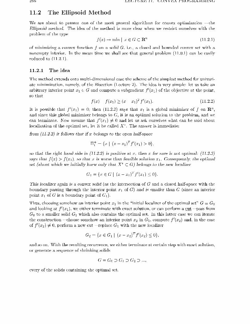
266 LECTURE 11. CONVEX PROGRAMMING
11.2 The Ellipsoid Method
We are about to present one of the most general algorithms for convex optimization { theEllipsoid method. The idea of the method is more clear when we restrict ourselves with theproblem of the type
f(x)! min j x 2 G � Rn (11.2.1)
of minimizing a convex function f on a solid G, i.e., a closed and bounded convex set with anonempty interior. In the mean time we shall see that general problem (11.0.1) can be easilyreduced to (11.2.1).
11.2.1 The idea
The method extends onto multi-dimensional case the scheme of the simplest method for univari-ate minimization, namely, of the Bisection (Lecture 2). The idea is very simple: let us take anarbitrary interior point x1 2 G and compute a subgradient f 0(x1) of the objective at the point,so that
f(x)� f(x1) � (x� x1)T f 0(x1): (11.2.2)
It is possible that f 0(x1) = 0; then (11.2.2) says that x1 is a global minimizer of f on Rn,and since this global minimizer belongs to G, it is an optimal solution to the problem, and wecan terminate. Now assume that f 0(x1) 6= 0 and let us ask ourselves what can be said aboutlocalization of the optimal set, let it be called X�. The answer is immediate:
from (11.2.2) it follows that if x belongs to the open half-space
�+1 = fx j (x� x1)
T f 0(x1) > 0g;so that the right hand side in (11.2.2) is positive at x, then x for sure is not optimal: (11.2.2)says that f(x) > f(x1), so that x is worse than feasible solution x1. Consequently, the optimalset (about which we initially knew only that X� � G) belongs to the new localizer
G1 = fx 2 G j (x� x1)T f 0(x1) � 0g:
This localizer again is a convex solid (as the intersection of G and a closed half-space with theboundary passing through the interior point x1 of G) and is smaller than G (since an interiorpoint x1 of G is a boundary point of G1).
Thus, choosing somehow an interior point x1 in the \initial localizer of the optimal set" G � G0
and looking at f 0(x1), we either terminate with exact solution, or can perform a cut { pass fromG0 to a smaller solid G1 which also contains the optimal set. In this latter case we can iteratethe construction { choose somehow an interior point x2 in G1, compute f 0(x2) and, in the caseof f 0(x2) 6= 0, perform a new cut { replace G1 with the new localizer
G2 = fx 2 G1 j (x� x2)T f 0(x2) � 0g;
and so on. With the resulting recurrence, we either terminate at certain step with exact solution,or generate a sequence of shrinking solids
G = G0 � G1 � G2 � :::;
every of the solids containing the optimal set.

11.2. THE ELLIPSOID METHOD 267
It can be guessed that if xt are chosen properly, then the localizers Gt \shrink to X� atcertain reasonable rate", and the method converges. This is, e.g., the case with Bisection: thereall Gt are segments (what else could be a solid on the axis?), and xt is chosen as the center ofGt�1; as a result, the lengths of the segments Gt go to 0 linearly with the ratio 1
2 , and since allthe localizers contain X�, the method converges at the same linear rate.
In multi-dimensional case the situation is much more diÆcult:
� the sets Gt can be more or less arbitrary solids, and it is not clear what does it mean a\center" of Gt, i.e., how to choose xt+1 2 Gt in order to achieve \signi�cant shrinkage" ofthe localizer at a step (by the way, how to measure this shrinkage?) On the other hand,it is clear that if xt+1 is badly chosen (e.g., is close to the boundary of Gt) and the newcut is \badly oriented", the next localizer Gt+1 may be \almost as large as Gt";
� in the one-dimensional case the linear sizes of the localizers tend to 0 linearly with ratio12 , and this is the source of convergence of xt to the minimizer of f . It is absolutely clearthat in the multi-dimensional case we cannot enforce the linear sizes of Gt to go to 0 (lookwhat happens if G = G0 is the unit square on the plane and f does not depend on the �rstcoordinate; in this case all localizers will be rectangles of the same width, and consequentlywe cannot enforce their linear sizes to go to 0). Thus, we should think carefully how tomeasure sizes of the localizers { with bad choice of the notion of size, we are unable topush it to 0.
The above remarks demonstrate that it is not that straightforward { to extend Bisection ontothe multi-dimensional case. Nevertheless, there are satisfactory ways to do it.
11.2.2 The Center-of-Gravity method
The �rst which comes to mind is to measure the sizes of the localizers as their n-dimensionalvolumes Vol(Gt) and to use, as xt+1, the center of gravity of Gt:
xt+1 =1
Vol(Gt)
ZGt
xdx:
A (very nontrivial) geometrical fact is that with this Center of Gravity policy we get linearconvergence of the volumes of Gt to 0:
Vol(Gt) ��1�
�n
n+ 1
�n�tVol(G0);
which in turn implies linear convergence in terms of the residual in the objective value: if xt isthe best { with the smallest value of the objective { of the points x1; :::; xt, then
f(xt)�minG
f ��1�
�n
n+ 1
�n�t=n[max
Gf �min
Gf ]: (11.2.3)
(11.2.3) demonstrates global linear convergence of the Center-of-Gravity method with objective-independent convergence ratio
�(n) =�1�
�n
n+ 1
�n�1=n� (1� expf�1g)1=n:

268 LECTURE 11. CONVEX PROGRAMMING
Consequently, to get an �-solution to the problem { to �nd a point xt 2 G with
f(xt)�minG
f � �[maxG
f �minG
f ]
{ it requires to perform no more than
c ln 1�
ln 1�(n)
b� 2:13n ln1
�+ 1 (11.2.4)
steps of the method2).Look how strong is the result: our global eÆciency estimate is objective-independent: no con-
dition numbers (and even no smoothness assumptions at all) are involved! f may be nonsmooth,may possess all kinds of degeneracy, etc., and all this does not in uence the estimate!
Let me add that the Center-of-Gravity method is, in certain precise sense, an optimal methodfor convex optimization.
A weak point of the method is the necessity to �nd, at every step, the center of gravity ofthe previous localizer. To �nd the center of gravity of a general type multi-dimensional solid(and even of a general type polytope) is, computationally, an extremely diÆcult problem. Ofcourse, if G (and then every Gt) is a polytope, this problem is \algorithmically solvable" { onecan easily point out a method which solves the problem in �nitely many arithmetic operations.Unfortunately, the number of arithmetic operations required by all known methods for �ndingthe center of gravity grows exponentially with n, so that are unable to compute centers of gravityin reasonable time already in the dimension 5-10. As a result, the Center-of-Gravity method isof \academic interest" only { it cannot be used as a computational tool.
11.2.3 From Center-of-Gravity to the Ellipsoid method
The Ellipsoid method can be viewed as certain \computationally tractable" approximation tothe Center-of-Gravity method. The idea is to enforce all the localizers to have \nice geometry"convenient for �nding the centers of gravity, namely, to be ellipsoids. Assume, e.g., that G0 = Gis an ellipsoid. Then there is no diÆculty to point out the center of G0, so that we have noproblems with the �rst step of the Center-of-Gravity method. Unfortunately, the resultinglocalizer, let it be called G+
1 , will be not an ellipsoid, but a \half-ellipsoid" { the intersection ofellipsoid G0 and a half-space with the boundary hyperplane passing through the center of G0;this solid is not that convenient for �nding the center of gravity. To restore the geometry of thelocalizer, let us cover the half-ellipsoid G+
1 by the ellipsoid of the smallest volume G1 containingG+1 , and let us take this G1 as our new localizer. Note that G1 indeed is a localizer of the
optimal set X� (since the latter is contained already in G+1 , and G1 covers G+
1 ). Now we arein the same situation as at the very beginning, but with G0 replaced with G1, and can iteratethe construction { to take the center x2 of the ellipsoid G1, to perform a new cut, getting a newhalf-ellipsoid G+
1 which covers the optimal set, to embed it into the ellipsoid G2 of the smallestpossible volume, etc. In this scheme, we actually make a kind of trade-o� between eÆciency ofthe routine and computational complexity of a step: when extending the \actual localizers" {half-ellipsoids { to ellipsoids, we add points which for sure could not be optimal solutions, andthus slow the procedure down. At the cost of this slowing the process down we, anyhow, enableourselves to deal with \simple sets" { ellipsoids, and thus reduce dramatically the computationalcomplexity of a step.
2here and in what follows we use the standard notation cab to denote the smallest integer � a real a

11.2. THE ELLIPSOID METHOD 269
There are two points which should be clari�ed.
� �rst, it is unclear in advance whether we indeed are able to decrease at linear rate thevolumes of sequential localizers and thus get a converging method { it could happenthat, when extending the half-ellipsoid G+
t+1 to the ellipsoid Gt+1 of the smallest volumecontaining G+
t+1, we come back to the previous ellipsoid Gt, so that no progress in volumeis achieved. Fortunately, this is not the case: the procedure reduces the volumes of thesequential ellipsoids Gt by factor ��(n) � expf� 1
2ng, thus enforcing the volumes of Gt
to go to 0 at linear rate with the ratio ��(n) 3). This ratio is worse than the one for theCenter-of-Gravity method (there the ratio was at most absolute constant 1�expf�1g, nowit is dimension-dependent constant close to 1� 1
2n); but we still have linear convergence!
� second, it was assumed that G is an ellipsoid. What to do if it is not so? The answeris easy: let us choose, as G0, an arbitrary ellipsoid which covers the domain G of theproblem; such a G0 for sure will be a localizer of the optimal set, and this is all we need.This answer is good, but there is a weak point: it may happen that the center x1 of theellipsoid G0 is outside G; how should we perform the �rst cut in this case? Moreover,this \bad" situation { when the center xt+1 of the current localizer Gt is outside G { mayeventually occur even when G0 = G is an ellipsoid: at each step of the method, we addsomething to the \half" of the previous localizer, and this something could contain pointsnot belonging to G. As a result, Gt, generally speaking, is not contained in G, and it mayhappen that the center of Gt is outside G. And to the moment we know how to performcuts only through points of G, not through arbitrary points of Rn.
We can immediately resolve the indicated diÆculty. Given the previous ellipsoidal localizerGt and its center xt+1, let us ask the Separation oracle whether xt+1 2 G. If it is the case,we have no problems with the cut { we call the First order oracle, get a subgradient of fat xt+1 and use it as it was explained above to produce the cut. Now, if xt+1 is not in G,the Separation oracle will return a separator e:
eTxt+1 > maxx2G
eTx:
Consequently, all the points x 2 G satisfy the inequality
(x� xt+1)T e < 0;
and we can use e for the cut, setting
G+t+1 = fx 2 Gt j (x� xt+1)
T e � 0g:
Since the inequality which \cuts G+t+1 o� Gt" is satis�ed on the entire G and, consequently,
on X�, and the latter set was assumed to belong to Gt (Gt is a localizer!), we concludethat X� � G+
t+1, and this is all we need.
After all explanations and remarks, we can pass to formal description of the Ellipsoid method.
3The fact that even after extending G+t+1 to Gt+1 we still have progress in volume heavily depends on the
speci�c geometrical properties of ellipsoids; if. e.g., we would try to replace the ellipsoids with boxes, we wouldfail to ensure the desired progress. The ellipsoids, anyhow, are not the only solids appropriate for our goals; wecould use simplexes as well, although with worse progress in volume per step

270 LECTURE 11. CONVEX PROGRAMMING
11.2.4 The Algorithm
How to represent an ellipsoid
An ellipsoid is a geometrical entity; to run an algorithm, we should deal with numerical repre-sentations of these entities. The most convenient for our goals is to represent an ellipsoid as theimage of the unit Euclidean ball under nonsingular aÆne mapping:
E = E(c;B) = fx = c+Bu j uTu � 1g: (11.2.5)
Here c 2 Rn is the center of the ellipsoid and B is an n�n nonsingular matrix. Thus, to say \anellipsoid" in what follows means exactly to say \the set (11.2.5) given by a pair (c;B) comprisedof vector c 2 Rn and a nonsingular n� n matrix B"; you may think about this representationas about the de�nition of an ellipsoid.
The volume the ellipsoid E(c; b) is
Vol(E(c;B)) = jDet Bjv(n);v(n) being the volume of the unit n-dimensional Euclidean ball Vn; indeed, E(c;B) is the imageof Vn under aÆne mapping, B being the matrix of the homogeneous part of the mapping, andsuch a transformation multiplies the volumes by jDet Bj.
We need the following simple
Lemma 11.2.1 Let n > 1, let
E = E(c;B) = fx = c+Bu j uTu � 1gbe an ellipsoid in Rn, and let
E+ = fx 2 E j (x� c)T e � 0g [e 6= 0]
be a "half-ellipsoid" { the intersection of E and a half-space with the boundary hyperplane passingthrough the center of E. Then E+ can be covered by ellipsoid E0 = E(c0; B0) of the volume
Vol(E0) = ��(n)Vol(E);
��(n) =n2
n2 � 1
sn� 1
n+ 1� expf� 1
2(n� 1)g: (11.2.6)
The parameters c0 and B0 of the ellipsoid E0 are given by
B0 = �(n)B � (n)(Bp)pT ; c0 = c� 1
n+ 1Bp; (11.2.7)
where
�(n) =
(n2
n2 � 1
)1=4
; (n) = �(n)
sn� 1
n+ 1; p =
BT epeTBBT e
:
To prove the lemma, it suÆces to reduce the situation to the similar one with E being theunit Euclidean ball V = Vn; indeed, since E is the image of V under the aÆne transformationu 7! Bu+ c, the half-ellipsoid E+ is the image, under this transformation, of the half-ball
V + = fu 2 V j (BT e)Tu � 0g = fu 2 V j pTu � 0g:

11.2. THE ELLIPSOID METHOD 271
Now, it is quite straightforward to verify that a half-ball indeed can be covered by an ellipsoidV 0 with the volume being the required fraction of the volume of V ; you may take
V 0 = fx j (x+ 1
n+ 1p)T [�(n)In � (n)ppT ]�2(x+
1
n+ 1p) � 1g:
It remains to note that the image of V 0 under the aÆne transformation which maps the unit ballV onto the ellipsoid E is an ellipsoid which clearly contains the half-ellipsoid E+ and is in thesame ratio of volumes with respect to E as V 0 is with respect to the unit ball V (since the ratio ofvolumes remains invariant under aÆne transformations). The ellipsoid E0 given in formulationof the lemma is nothing but the image of the above V 0 under our aÆne transformation.
The Ellipsoid algorithm
The algorithm is as follows
Algorithm 11.2.1 [The Ellipsoid algorithm for convex program f(x)! min j x 2 G � Rn]Assumptions:
� G is a solid (bounded and closed convex set with a nonempty interior)
� we are given First order oracle for f and Separation oracle for G
� we are able to point out an ellipsoid G0 = E(c0; B0) which contains G.
Initialization: set t = 1Step t: Given ellipsoid Gt�1 = E(ct�1; Bt�1), set xt = ct�1 and act as follows:
1) [Call the Separation Oracle] Call the Separation oracle, xt being the input. If the oraclesays that xt 2 G, call the step t productive and go to 2), otherwise call the step t non-productive,set et equal to the separator returned by the oracle:
x 2 G) (x� xt)T et < 0
and go to 3)2) [Call the First order oracle] Call the First order oracle, xt being the input. If f 0(xt) = 0,
terminate { xt 2 G is the minimizer of f on the entire Rn (see the de�nition (11.1.1) of asubgradient) and is therefore an optimal solution to the problem. In the case of f 0(xt) 6= 0 set
et = f 0(xt)
and go to 3).3) [Update the ellipsoid] Update the ellipsoid E(ct�1; Bt�1) into E(ct; Bt) according to for-
mula (11.2.7) with e = et, i.e., set
Bt = �(n)Bt�1 � (n)(Bt�1pt)pTt ; ct = ct�1 � 1
n+ 1Bt�1pt�1;
where
�(n) =
(n2
n2 � 1
)1=4
; (n) = �(n)
sn� 1
n+ 1; pt =
BTt�1etq
eTt Bt�1BTt�1et
:
Replace t with t+ 1 and go to the next step.Approximate solution xt generated by the method after t steps is, by de�nition, the best (withthe smallest value of f0) of the points xj generated at the productive steps j � t [if the steps1; :::; t are non-productive, xt is unde�ned].

272 LECTURE 11. CONVEX PROGRAMMING
11.2.5 The Ellipsoid algorithm: rate of convergence
We are about to prove the main result on the Ellipsoid method.
Theorem 11.2.1 [Rate of convergence of the Ellipsoid algorithm]Let n > 1, and let convex program (11.2.1) satisfying the assumptions from the description ofthe Ellipsoid algorithm 11.2.1 be solved by the algorithm. Let
N(�) =c2n(n� 1) ln�V�
�b;
where 0 < � < 1 and
V =�Vol(E(c0; B0))
Vol(G)
�1=nThen, for any � 2 (0; 1), the approximate solution xN(�) found by the method in course of the �rstN(�) steps, is well-de�ned and is an �-solution to the problem, i.e., belongs to G and satis�esthe inequality
f(xN(�))�minG
f � �[maxG
f �minGf ]: (11.2.8)
Proof. For the sake of brevity, let N = N(�). We may assume that the method does notterminate in course of the �rst N steps { otherwise there is nothing to prove: the only possibilityfor the method to terminate is to �nd an exact optimal solution to the problem.
Let us �x �0 2 (�; 1), and let x� be an optimal solution to (11.2.1) (it exists, since the domainof the problem is compact and the objective, being convex on Rn, is continuous (we had such atheorem in the course Optimization I) and therefore attains its minimum on compact set G.10. Set
G� = x� + �0(G� x�);
so that G� is the image of G under homothety transformation with the center at x� and thecoeÆcient �0.
By construction, we have
Vol(G�) = (�0)nVol(G) > �nVol(G) (11.2.9)
(\homothety with coeÆcient � > 0 in Rn multiplies volumes by �n"). On the other hand, byLemma 11.2.1 we have Vol(E(ct; Bt)) � expf�1=(2(n � 1))gVol(E(ct�1; Bt�1)), whence
Vol(E(cN ; BN ) � expf� N
2(n� 1)gVol(E(c0; B0)) �
[de�nition of N = N(�)]� V�N�N Vol(E(c0; B0)) =
[de�nition of V]=
Vol(G)
Vol(E(c0; B0))�N Vol(E(c0; B0)) = �N Vol(G):
Comparing the resulting inequality with (11.2.9), we conclude that Vol(E(cN ; BN )) < Vol(G�),so that
G�nE(cN ; BN ) 6= ;: (11.2.10)
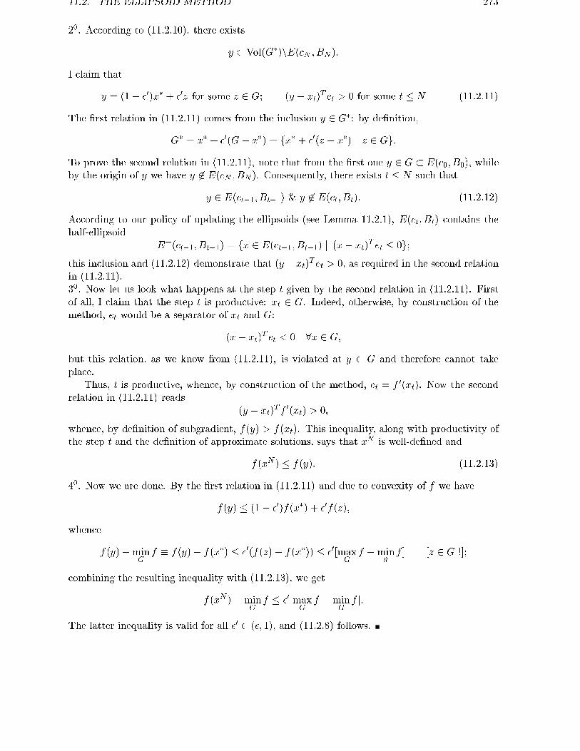
11.2. THE ELLIPSOID METHOD 273
20. According to (11.2.10), there exists
y 2 Vol(G�)nE(cN ; BN ):
I claim that
y = (1� �0)x� + �0z for some z 2 G; (y � xt)T et > 0 for some t � N (11.2.11)
The �rst relation in (11.2.11) comes from the inclusion y 2 G�: by de�nition,
G� = x� + �0(G� x�) = fx� + �0(z � x�) j z 2 Gg:To prove the second relation in (11.2.11), note that from the �rst one y 2 G � E(c0; B0), whileby the origin of y we have y 62 E(cN ; BN ). Consequently, there exists t � N such that
y 2 E(ct�1; Bt�1) & y 62 E(ct; Bt): (11.2.12)
According to our policy of updating the ellipsoids (see Lemma 11.2.1), E(ct; Bt) contains thehalf-ellipsoid
E+(ct�1; Bt�1) = fx 2 E(ct�1; Bt�1) j (x� xt)T et � 0g;
this inclusion and (11.2.12) demonstrate that (y�xt)T et > 0, as required in the second relationin (11.2.11).30. Now let us look what happens at the step t given by the second relation in (11.2.11). Firstof all, I claim that the step t is productive: xt 2 G. Indeed, otherwise, by construction of themethod, et would be a separator of xt and G:
(x� xt)T et < 0 8x 2 G;
but this relation, as we know from (11.2.11), is violated at y 2 G and therefore cannot takeplace.
Thus, t is productive, whence, by construction of the method, et = f 0(xt). Now the secondrelation in (11.2.11) reads
(y � xt)T f 0(xt) > 0;
whence, by de�nition of subgradient, f(y) > f(xt). This inequality, along with productivity ofthe step t and the de�nition of approximate solutions, says that xN is well-de�ned and
f(xN ) � f(y): (11.2.13)
40. Now we are done. By the �rst relation in (11.2.11) and due to convexity of f we have
f(y) � (1� �0)f(x�) + �0f(z);
whence
f(y)�minG
f � f(y)� f(x�) � �0(f(z)� f(x�)) � �0[maxG
f �mingf ] [z 2 G !];
combining the resulting inequality with (11.2.13), we get
f(xN )�minG
f � �0[maxG
f �minG
f ]:
The latter inequality is valid for all �0 2 (�; 1), and (11.2.8) follows.

274 LECTURE 11. CONVEX PROGRAMMING
11.2.6 Ellipsoid method for problems with functional constraints
To the moment we spoke about the Ellipsoid method as applied to problem (11.2.1) withoutfunctional constraints. There is no diÆculty to extend the method onto general convex problems(11.0.1). To this end it suÆces to note that (11.0.1) can be immediately rewritten as problemof the type (11.2.1), namely, as
f(x) � f0(x)! min j x 2 G � fx 2 G j fi(x) � 0; i = 1; :::;mg: (11.2.14)
All we need to solve this latter problem by the Ellipsoid algorithm is
� to equip (11.2.14) by the Separation and the First order oracles
this is immediate: the First order oracle for (11.2.14) is readily given by the one for (11.0.1).The Separation oracle for G can be immediately constructed from the Separation oraclefor G and the First order oracle for (11.0.1): given x 2 Rn, we �rst check whether thepoint belongs to G, If it is not the case, then it, of course, does not belong to G as well,and the separator (given by the Separation oracle for G on the input x) separates x fromG. Now, if x 2 G, we can ask the First order oracle about the values and subgradients off1; :::; fm at x. If all the values are nonpositive, then x 2 G; if one of this values is positive,then x 62 G and, moreover, the vector f 0i(x) (i � 1 is such that fi(x) > 0) can be used asa separator of x and G (Remark 11.1.1)
� to ensure that G is a solid
(we shall simply assume this).
The resulting algorithm is as follows
Algorithm 11.2.2 [The Ellipsoid algorithm for convex program (11.0.1)]Assumptions:
� G = fx 2 G j fi(x) � 0; i = 1; :::;mg is a solid (bounded and closed convex set with anonempty interior)
� we are given First-order oracle for f0; :::; fm and Separation oracle for G
� we are able to point out an ellipsoid G0 = E(c0; B0) which contains G.
Initialization: set t = 1Step t: Given ellipsoid Gt�1 = E(ct�1; Bt�1), set xt = ct�1 and act as follows:
1) [Call the Separation oracle] Call the Separation oracle for G, xt being the input. If theoracle says that xt 2 G, go to 2), otherwise call the step t non-productive, set et equal to theseparator returned by the oracle:
x 2 G) (x� xt)T et < 0
and go to 4)2) [Call the First order oracle] Call the First order oracle, xt being the input, and check
whether fi(xt) � 0, i = 1; :::;m. If fi(xt) � 0 for all i � 1, call the step t productive and lookat f 00(xt). If f
00(xt) = 0, terminate { xt is feasible for (11.0.1) and is the minimizer of f on the

11.3. ELLIPSOID METHOD AND COMPLEXITY OF CONVEX PROGRAMMING 275
entire Rn (see the de�nition (11.1.1) of a subgradient), whence it is an optimal solution to theproblem. In the case of f 00(xt) 6= 0 set
et = f 00(xt)
and go to 4).3) [The case of xt 2 G and fi(xt) > 0 for some i � 1] Call step t non-productive and �nd
i � 1 such that fi(xt) > 0 (when we arrive at 3), such an i exists), set
et = f 0i(xt)
and go to 4).4) [Updating the ellipsoid] Update the ellipsoid E(ct�1; Bt�1) into E(ct; Bt) according to
formula (11.2.7) with e = et, i.e., set
Bt = �(n)Bt�1 � (n)(Bt�1pt)pTt ; ct = ct�1 � 1
n+ 1Bt�1pt�1;
where
�(n) =
(n2
n2 � 1
)1=4
; (n) = �(n)
sn� 1
n+ 1; pt =
BTt�1etq
eTt Bt�1BTt�1et
:
Replace t with t+ 1 and go to the next step.Approximate solution xt generated by the method after t steps is, by de�nition, the best (with thesmallest value of f) of the points xj generated at the productive steps j � t [if the steps 1; :::; tare non-productive, xt is unde�ned].
The following result is an immediate corollary of Theorem 11.2.1.
Theorem 11.2.2 [Rate of convergence of the Ellipsoid algorithm on problems with functionalconstraints]Let n > 1, and let convex program (11.0.1) satisfying the assumptions from the description ofthe Ellipsoid algorithm 11.2.2 be solved by the algorithm. Let
N(�) =c2n(n� 1) ln�V�
�b;
where 0 < � < 1 and
V =
"Vol(E(c0; B0))
Vol(G)
#1=nThen, for any � 2 (0; 1), the approximate solution xN(�) found by the method in course of the �rstN(�) steps, is well-de�ned and is an �-solution to the problem, i.e., belongs to G and satis�esthe inequality
f(xN(�))�minG
f � �[maxG
f �minGf ]: (11.2.15)
11.3 Ellipsoid method and Complexity of Convex Programming
The Ellipsoid method implies fundamental theoretical results on complexity of Convex Program-ming; let us brie y discuss these theoretical issues.

276 LECTURE 11. CONVEX PROGRAMMING
11.3.1 Complexity: what is it?
When speaking about complexity of a class of computational problems, we are interested toanswer the following crucial question:
Given a family P of problem instances and required accuracy �, what can be said about thecomputational e�ort suÆcient to solve each instance to the prescribed accuracy?
This is an informal question, of course, and to answer it, we should �rst formalize the questionitself, namely, to say
� What does it mean \a family of problems" and how we measure accuracy of approximatesolutions;
� What does it mean \e�ort of computational process"? What is the model of the processand how the e�ort is measured?
To realize that these indeed are points which should be clari�ed, consider the following \uni-versal solution method" (which in fact is the main method to solve problems): think! Is it a\computational method"? What is the \e�ort" for this method?
There are basically two approaches to formalize the complexity-related notions. The �rst,which is more convenient for \continuous" computational problems, is as follows (according toour goals, I shall speak only about optimization problems in the form (11.2.1)).
Real Arithmetic Complexity Model:
� A family of problems P is a set of problems (11.2.1) such that a particular member p =(f;G) of the family is encoded by a �nite-dimensional data vector d(p). The dimension ofthe data vector is called the size of the instance.
Example 1. Linear Programming over Reals. Here the instances are of the form
f(x) = cTx! min j x 2 G = fx 2 Rn j Ax � bg;
A being m � n matrix and b being m-dimensional vector. The data vector of a probleminstance is comprised of the pair n;m and of n+m+nm entries of c, b, A written down ina once for ever �xed order (e.g., �rst the n entries of c, then the m entries of b and �nallythe nm entries of A in the row-wise order).
Example 2. Quadratically Constrained Quadratic Programming. Here the in-stances are of the form
f0(x) =1
2xTH0x� bT0 x! min
subject to
x 2 G = fx 2 Rn j fi(x) = 1
2xTHix� bTi x+ ci � 0; i = 1; :::;mg;
and the data vector is comprised of n, m and the entries of the matrices Hi, the vectorsbi and the reals ci written down in a once for ever �xed order.
The number of examples can be easily extended; basically, the typical families of problemsin question are comprised of problems of a \�xed generic analytical structure", and the
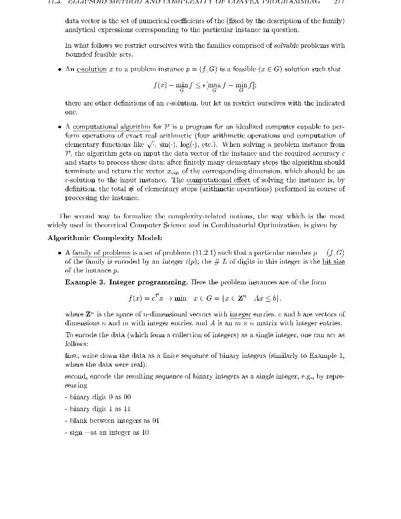
11.3. ELLIPSOID METHOD AND COMPLEXITY OF CONVEX PROGRAMMING 277
data vector is the set of numerical coeÆcients of the (�xed by the description of the family)analytical expressions corresponding to the particular instance in question.
In what follows we restrict ourselves with the families comprised of solvable problems withbounded feasible sets.
� An �-solution x to a problem instance p = (f;G) is a feasible (x 2 G) solution such that
f(x)�minG
f � �[maxG
f �minG
f ];
there are other de�nitions of an �-solution, but let us restrict ourselves with the indicatedone.
� A computational algorithm for P is a program for an idealized computer capable to per-form operations of exact real arithmetic (four arithmetic operations and computation ofelementary functions like
p�, sin(�), log(�), etc.). When solving a problem instance fromP, the algorithm gets on input the data vector of the instance and the required accuracy �and starts to process these data; after �nitely many elementary steps the algorithm shouldterminate and return the vector xout of the corresponding dimension, which should be an�-solution to the input instance. The computational e�ort of solving the instance is, byde�nition, the total # of elementary steps (arithmetic operations) performed in course ofprocessing the instance.
The second way to formalize the complexity-related notions, the way which is the mostwidely used in theoretical Computer Science and in Combinatorial Optimization, is given by
Algorithmic Complexity Model:
� A family of problems is a set of problems (11.2.1) such that a particular member p = (f;G)of the family is encoded by an integer i(p); the # L of digits in this integer is the bit sizeof the instance p.
Example 3. Integer programming. Here the problem instances are of the form
f(x) = cTx! min j x 2 G = fx 2 Zn j Ax � bg;where Zn is the space of n-dimensional vectors with integer entries, c and b are vectors ofdimensions n and m with integer entries, and A is an m� n matrix with integer entries.
To encode the data (which form a collection of integers) as a single integer, one can act asfollows:
�rst, write down the data as a �nite sequence of binary integers (similarly to Example 1,where the data were real);
second, encode the resulting sequence of binary integers as a single integer, e.g., by repre-senting
- binary digit 0 as 00
- binary digit 1 as 11
- blank between integers as 01
- sign { at an integer as 10

278 LECTURE 11. CONVEX PROGRAMMING
Example 4. Linear Programming over Rationals. This is a subfamily of the Lin-ear Programming family (Example 1), where we impose on all the entries of c; b; A therequirement to be rational numbers. To encode a problem instance by a single binaryinteger, it suÆces to write the data as a sequence of binary integers, same as in Example3 (with the only di�erence that now every rational element of the data is represented bytwo sequential integers, its numerator and denominator), and then encode the sequence,as it was explained above, by a single binary integer.
In what follows, speaking about Algorithmic Complexity model, we always assume that
- the families in question are comprised of solvable problems with bounded feasible sets
- any problem instance from the family admits a solution which can be naturally encodedby a binary integer
The second assumption is clearly valid for the Integer Programming (Example 3). It is alsovalid for Linear Programming over Rationals (Example 4), since it can be easily provedthat a solvable LP program with integer data admits a solution with rational entries; andwe already know that any �nite sequence of integers/rationals can be naturally encodedby a single integer.
� Normally, in Algorithmic Complexity model people are not interested in approximatesolutions and speak only about exact ones; consequently, no problem with measuringaccuracy occurs.
� A computational algorithm is an algorithm in any of (the equivalent to each other) def-initions given in Mathematical Logic; you loose nothing when thinking of a program foran idealized computer which is capable to store in memory as many �nite binary words asyou need and to perform bit-wise operations with these words. The algorithm as appliedto a problem instance p from P gets on input the code i(p) of the instance and starts toprocess it; after �nitely many elementary steps, the algorithm should terminate and returnthe code of an exact solution to the instance. The computational e�ort is measured as thetotal # of elementary bit-wise operations performed in course of the solution process.
Let me stress the di�erence between the notions of the size of an instance in the RealArithmetic and the Algorithmic Complexity models. In the �rst model, the size of an instanceis, basically, the # of real coeÆcients in the natural analytical representation of the instance,and the size is independent of the numerical values of these coeÆcients { they may be arbitraryreals. E.g. the Real Arithmetic size of any LP program over Reals (Example 1) with n = 2variables and m = 3 inequality constraints is the dimension of the vector
(2; 3; c1; c2; b1; b2; b3; A11; A12; A21; A22; A31; A32);
i.e., 13. In contrast to this, the Algorithmic Complexity size of an LP program over Rationals(Example 4) with n = 2 variables and m = 3 constraints can be arbitrarily large, if the rationaldata are \long".
We can observe similar di�erence between the measures of computational e�ort in the RealArithmetic and the Algorithmic Complexity models. In the �rst of them, the e�ort required,say, to add two reals is one, independently of what the reals are. In the second model, we inprinciple cannot deal with reals { only with integers; and the e�ort to add two N -digit integersis not 1 { it is proportional to N .
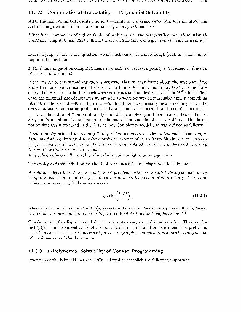
11.3. ELLIPSOID METHOD AND COMPLEXITY OF CONVEX PROGRAMMING 279
11.3.2 Computational Tractability = Polynomial Solvability
After the main complexity-related notions { family of problems, �-solution, solution algorithmand its computational e�ort { are formalized, we may ask ourselves
What is the complexity of a given family of problems, i.e., the best possible, over all solution al-gorithms, computational e�ort suÆcient to solve all instances of a given size to a given accuracy?
Before trying to answer this question, we may ask ourselves a more rough (and, in a sense, moreimportant) question:
Is the family in question computationally tractable, i.e. is its complexity a \reasonable" functionof the size of instances?
If the answer to this second question is negative, then we may forget about the �rst one: if weknow that to solve an instance of size l from a family P it may require at least 2l elementarysteps, then we may not bother much whether the actual complexity is 2l, 25l or 2(2
l): in the �rstcase, the maximal size of instances we are able to solve for sure in reasonable time is somethinglike 30, in the second { 6, in the third { 5; this di�erence normally means nothing, since thesizes of actually interesting problems usually are hundreds, thousands and tens of thousands.
Now, the notion of \computationally tractable" complexity in theoretical studies of the last30 years is unanimously understood as the one of \polynomial time" solvability. This latternotion �rst was introduced in the Algorithmic Complexity model and was de�ned as follows:
A solution algorithm A for a family P of problem instances is called polynomial, if the compu-tational e�ort required by A to solve a problem instance of an arbitrary bit size L never exceedsq(L), q being certain polynomial; here all complexity-related notions are understood accordingto the Algorithmic Complexity model.P is called polynomially solvable, if it admits polynomial solution algorithm.
The analogy of this de�nition for the Real Arithmetic Complexity model is as follows:
A solution algorithms A for a family P of problem instances is called R-polynomial, if thecomputational e�ort required by A to solve a problem instance p of an arbitrary size l to anarbitrary accuracy � 2 (0; 1) never exceeds
q(l) ln�V(p)
�
�; (11.3.1)
where q is certain polynomial and V(p) is certain data-dependent quantity; here all complexity-related notions are understood according to the Real Arithmetic Complexity model.
The de�nition of an R-polynomial algorithm admits a very natural interpretation. The quantityln(V(p)=�) can be viewed as # of accuracy digits in an �-solution; with this interpretation,(11.3.1) means that the arithmetic cost per accuracy digit is bounded from above by a polynomialof the dimension of the data vector.
11.3.3 R-Polynomial Solvability of Convex Programming
Invention of the Ellipsoid method (1976) allowed to establish the following important

280 LECTURE 11. CONVEX PROGRAMMING
Theorem 11.3.1 [R-polynomial solvability of Convex Programming]
Consider a family P of convex problems (11.2.1) and assume that(i) all problem instances p = (f;G) from the family are bounded (i.e., their feasible domains
G are bounded) and strictly feasible (i.e., their feasible domains G possess nonempty interiors);moreover, given the data vector d(p) of the instance, one can in polynomial in the size lp =dim d(p) of the instance number of arithmetic operations compute an ellipsoid which covers Galong with a lower bound vp > 0 for the volume of G;
(ii) given an instance p = (f;G) 2 P and a point x 2 Rnp , np being the # of variables in p,on can in polynomial in lp number of arithmetic operations
� imitate the Separation oracle for G on the input x, i.e., check the inclusion x 2 G and, ifit is not valid, compute a separator e:
supy2G
eT y < eTx;
� imitate the First order oracle for f , i.e., compute f(x) and f 0(x).
Then there exists an R-polynomial algorithm for P.
Proof is immediate: it suÆces to use the Ellipsoid algorithm. Indeed,
� (i) says that, given on input the data vector d(p) of a problem instance p 2 P, we canin polynomial in lp = dim d(p) number of arithmetic operations compute an ellipsoidE(c0; B0) and thus start the Ellipsoid algorithm. As a byproduct, we observe that thenumber of variables np in p is bounded from above by a polynomial of the size lp of theinstance (otherwise it would require too many operations simply to write down the centerof the ellipsoid).
� according to the description of the method, to perform a step of it, we should imitate theSeparation and, possibly, the First order oracle at current point xt (according to (iii), ittakes polynomial in lp number of arithmetic operations) and then should perform O(n2p)arithmetic operations to update the previous ellipsoid into the current one according toAlgorithm 11.2.1.3); by virtue of the previous remark, np is bounded from above by apolynomial in lp, so that the overall arithmetic e�ort at a step is polynomial in lp;
� according to Theorem 11.2.1, the method will �nd an �-solution to p in the number ofsteps not exceeding
N(�) =c2(np � 1)np ln�V�
�b; V =
�Vol(E(c0; B0))
Vol(G)
�1=np;
we have
N(�) � N 0(�) =c2(np � 1)np ln
Vol1=np(E(c0; B0))
v1=npp �
!b
(see (i)); according to (i), we can compute N 0(�) in polynomial in lp number of operationsand terminate the process after N 0(p) steps, thus getting an �-solution to p.

11.4. POLYNOMIAL SOLVABILITY OF LINEAR PROGRAMMING 281
The overall arithmetic e�ort to �nd an �-solution to p, in view of the above remarks, is boundedfrom above by
r(lp)N0(�) � q(lp) ln
�V(p)�
�; V(p) �
"Vol(E(c0; B0))
vp
#1=np;
both r(�) and q(�) being certain polynomials, so that the presented method indeed is R-polynomial.
When thinking of Theorem 11.3.1, you should take into account that the \unpleasant" as-sumptions (i) are completely technical and normally can be ensured by slight regularization ofproblem instances. Assumption (ii) is satis�ed in all \non-pathological" applications, so thatin fact Theorem 11.3.1 can be quali�ed as a General Theorem on R-Polynomial Solvability ofConvex Programming. I should add that this is, in a sense, an \existence theorem": it claimsthat in Convex Programming there exists a \universal" R-polynomial solution routine, but itdoes not say that this is the best possible R-polynomial routine for all particular cases. Themain practical drawback of the Ellipsoid method is that it is \slow" { the # of iterations re-quired to solve the problem within a once for ever �xed accuracy � grows quadratically withthe dimension n of the problem. This quadratic in n growth of the e�ort makes it basicallyimpossible to use the method as a practical tool in dimensions like hundreds and thousands.Recently, for many important families of Convex Programming problems (Linear, QuadraticallyConstrained Quadratic, Geometric and some others) more specialized and more eÆcient inte-rior point polynomial algorithms were developed; these methods are capable to struggle withlarge-scale problems of real-world origin.
I would say that the Ellipsoid method, as a practical tool, is �ne for not large { up to 20-30variables { convex problems. The advantages of the method are:
� simplicity in implementation and good numerical stability
� universality
� low order of dependence of computational e�ort on m { the # of functional constraints
The latter remark relates to Algorithm 11.2.2): the number of steps required to achieve agiven accuracy is simply independent ofm, and the e�ort per step is at most proportional tothem (the only place where the number of constraints in uence the e�ort is the necessity tocheck feasibility of the current iterate and to point out a violated constraint, if any exists).As a result, for \high and narrow" convex programs (say, with up to 20-30 variables andas many thousands of constraints as you wish) the Ellipsoid method seems to be one ofthe best known Convex Programming routines.
11.4 Polynomial solvability of Linear Programming
Surprisingly, the most important \complexity consequences" of the Ellipsoid method { whichis a purely \continuous optimization" algorithm { relate to Algorithmic Complexity. The mostknown of these consequences is

282 LECTURE 11. CONVEX PROGRAMMING
11.4.1 Polynomial Solvability of Linear Programming over Rationals
Some History
Everybody knows that Linear Programming programs { both with real and rational data { canbe solved eÆciently (and are solved almost for 50 years) by the Simplex Algorithm, which isa �nite Real Arithmetic routine for LP capable to solve huge practical linear programs. WhatI am not sure is that everybody knows what does it mean \eÆciently" in the above sentence.This is practical eÆciency { when solving an LP program
cTx! min j Ax � b (11.4.1)
with n variables and m > n inequality constraints, the Simplex normally performs 2m - 4miterations to �nd the solution. Anyhow, theoretically Simplex is not a polynomial algorithm:since the beginning of sixties, it is known that there exist simple LP programs pn with n =1; 2; 3; ::: variables and integer data of the total bit size Ln = O(n2) such that some versionsof the Simplex method solve pn in no less than 2n steps. Consequently, the aforementionedversions of the Simplex method are not polynomial { for a polynomial algorithm, the solutiontime should be bounded by a polynomial of Ln = O(n), i.e., of n. Similar \bad examples" wereconstructed for other versions of the Simplex method; and although nobody was able to provethat no version of Simplex can be polynomial, nobody was also lucky to point out a polynomialversion of the Simplex method. Moreover, since mid-sixties, where the Algorithmic Complexityapproach became standard, and till 1979 nobody knew whether LP over Rationals (Example 4above) is or is not polynomially solvable.
11.4.2 Khachiyan's Theorem
The positive answer on the fundamental question whether LP over Rationals is polynomiallysolvable was given only in 1979 by L. Khachiyan; the main tool used in the proof was theEllipsoid method invented 3 years earlier.
Below I sketch the reasoning of Khachiyan.
Step 1: from Optimization to Feasibility
The �rst step of the construction reduces the optimization LP program (11.4.1) to the Feasibilityprogram for a system of linear inequalities. To this end it suÆces to write down both theinequalities of (11.4.1) and of its LP dual and to replace minimization in the primal problemand maximization in the dual one with the linear constraint that the duality gap should be zero.This results in the following system of linear inequalities and equations:
Ax � b; AT y = c; y � 0; cTx = bT y (11.4.2)
with unknowns x 2 Rn and y 2 Rm. The Duality Theorem in Linear Programming says thatthe original problem (11.4.1) is solvable if and only if (11.4.2) is, and if it is the case, thenx-components of the solutions to (11.4.2) are exactly the optimal solutions to (11.4.1).
Assembling x and y in a single vector of variables u, representing u as the di�erence of newnonnegative variable vectors v and w and, �nally, assembling v and w into single vector z (allthese manipulations are standard tricks in LP),
we can rewrite (11.4.2) equivalently as the problem
�nd z 2 RN : Qz � q; z � 0; (11.4.3)

11.4. POLYNOMIAL SOLVABILITY OF LINEAR PROGRAMMING 283
here N = 2(n+m), and Q, q are certain matrix and vector with rational entries coming, in anevident fashion, from the initial data c; b; A. Note that the bit size L1 of the data in (11.4.3) isof order of the bit size L of the initial data in (11.4.1); in fact L1 � 10L.
It is convenient to pass from problem (11.4.3) with rational data to an equivalent problemwith integer data; to this end it suÆces to compute the common denominator of all the fractionsinvolved into (11.4.3) and to multiply all the data by this common denominator. As a result,we come to the problem
�nd x 2 RN : Rz � r; z � 0; (11.4.4)
the properties of this problem are as follows:
� (11.4.3) is equivalent to the LP program (11.4.1): both the problems are solvable/unsolvablesimultaneously; if they are solvable, then any solution to (11.4.4) can be converted in anexplicit and simple manner into optimal solution to (11.4.1);
� the data in (11.4.4) are integer, and their bit size L2 is bounded by a polynomial (somethinglike 200L2) of the bit size L of the initial data 4).
It follows that if we were able to solve in polynomial time the Feasibility problem (11.4.4), wewould get, as a byproduct, a polynomial algorithm for the initial problem (11.4.1).
Step 2: from Feasibility to Solvability
Instead of attacking the Feasibility problem (11.4.4) (where we are asked to check whether(11.4.4) is solvable and if it is the case { are asked to point out a solution), let us for the timebeing restrict our goals with the following relaxed solvability version of (11.4.4):
(S) given the data of (11.4.4), detect whether the problem is solvable.
The simpli�cation, as compared to (11.4.4), is that now we are not obliged to point out anexplicit solution to a solvable instance.
Problem (S) is the problem which is solved in polynomial time by the Ellipsoid method.This is done as follows.
� From (S) to (S0). Problem (S) clearly is equivalent to the following optimization problem:let
f(z) = max [(Rz)1 � r1j; (Rz)2 � r2; :::; (Rz)M � rM j](M is the number of rows in R) be the residual function of the system of inequalitiesRz � r; this function clearly is nonnegative at a nonnegative z if and only if z is a feasiblesolution to (11.4.4). Consequently, (S) is exactly the following problem:
(S0): detect whether minz2RN ;z�0 f(z) � 0
((S) is solvable if and only if the answer in (S0) is \yes").
� From (S0) to (S00). The next step is given by the following simple4the latter property comes from the fact that the common denominator of the entries in (11.4.3) is an integer
of bit size at most L1 � 10L; therefore when passing from (11.4.3) to (11.4.4), we increase the bit size of eachentry by at most 10L. Since even the total bit size of the entries in (11.4.3) is at most 10L, the bit size of anentry in (11.4.4) is at most 20L; and there are at most 10L entries. All our estimates are extremely rough, but itdoes not matter { all we are interested in is to ensure polynomiality of the bit size of the transformed problem inthe bit size of the initial one

284 LECTURE 11. CONVEX PROGRAMMING
Lemma 11.4.1 The answer in (S0) is \yes" if and only if it is \yes" in the followingproblem
(S00) detect whether minz:0�zi�2L2 ; i=1;:::;N f(z) � 0
L2 being the bit length of the data in (S).
Proof. If the answer in (S00) is \yes", then, of course, the answer in (S0) also is \yes".It remains to prove, therefore, that if the answer in (S0) is \yes" (or, which is the same,if (S) is solvable), then the answer in (S00) also is \yes". This is easy. The solutionset of (S), being nonempty, is a nonempty closed convex polyhedral set (here and in whatfollows I use the standard terminology of Convex Analysis; this terminology, along with allrequired facts, was presented in the course Optimization I); since (S) involves nonnegativityconstraints, this set does not contain lines, and therefore, due to the well-known fact ofConvex Analysis, possesses an extreme point �z. From the standard facts on the structureof extreme points of a polyhedral set given by (11.4.4) it is known that the vector z�
comprised of nonzero entries of �z, if such entries exist, satisfy nonsingular system of linearequations of the form
�Rz� = �r;
where
{ �R is a k � k nonsingular submatrix in R (k is the # of nonzero entries in �z)
{ �r is certain fragment of the right hand side vector r
(R and r are given by (11.4.4)).
It follows that the entries in z� are given by the Cramer rules { they are ratios of certaink � k determinants taken from the k � (k + 1) matrix [ �Rj�r]:
z�i =�i
�0:
All entries in this matrix are integers, and the total bit size of the entries does not exceedL2. It follows that all the determinants are, in absolute value, at most 2L2 5). Thus, thenumerators in the Cramer formulae are � L2 in absolute values, while the denominator(being a nonzero integer) is in absolute value � 1. Consequently, jz�i j � 2L2 .
Thus, all nonzero entries in �z are � 2L2 in absolute values. Since �z is a solution to (S),this is a point where f is nonnegative. We conclude that if the answer in (S) is \yes", thenf attains nonpositive value in the box 0 � zi � 2L2 , 1 � i � N , so that the answer in (S00)also is \yes".
5This is a consequence of the Hadamard inequality: the absolute value of a determinant (� the volume of theparallelotope spanned by the rows of the determinant) does not exceed the product of the Euclidean lengths ofthe rows of the determinant (product of the edges of the parallelotope). Consequently, log2j�ij does not exceedthe sum of binary logs of the Euclidean lengths of the rows of [ �Rj�r]. It remains to note that the binary logarithmof the Euclidean length of an integer vector clearly does not exceed the total bit length of the vector:
1
2log2(a
21 + :::+ a2k) � 1
2log2[(1 + a21)(1 + a2)
2:::(1 + a2k)] =
kXi=1
1
2log2[1 + a2i ] �
kXi=1
log2[1 + jaij]
and the latter expression clearly is � the total # of binary digits in integers a1; :::; ak.

11.4. POLYNOMIAL SOLVABILITY OF LINEAR PROGRAMMING 285
� (S00) as a convex program. To solve problem (S00) is exactly the same as to checkwhether the optimal value in the optimization program
f(z)! min j z 2 G = fz 2 Rn j 0 � zi � 2L2 ; i = 1; :::; Ng (11.4.5)
is or is not positive. The objective in the problem is easily computable convex function(since it is maximum of M linear forms), and the domain G of the problem is a simplesolid - a box. Remark 11.1.1 explains how to imitate the First order and the Separationoracles for the problem; we can immediately point out the initial ellipsoid which containsG (simply the Euclidean ball circumscribed around the cube G). Thus, we are able to solvethe problem by the Ellipsoid method. From Theorem 11.2.1 (where one should estimatethe quantities V and maxG f � minG f via L2; this is quite straightforward) it followsthat in order to approximate the optimal value f� in (11.4.5) within a prescribed absoluteaccuracy � > 0, it suÆces to perform
N� = O(1)N2[L2 + ln1
�]
steps with at most O(1)(M +N)N arithmetic operations per step, which gives totally
M(�) = O(1)N3(M +N)[L2 + ln1
�] (11.4.6)
arithmetic operations (O(1) here and in what follows are positive absolute constants).
All this looks �ne, but in order to detect whether the optimal value f� in (11.4.5) is or isnot nonpositive (i.e., whether (S) is or is not solvable), we should distinguish between two\in�nitesimally close to each other" hypotheses f� � 0 and f� > 0, which seems to requirethe exact value of f�; and all we can do is to approximate \quickly" f� to a prescribedaccuracy � > 0, not to �nd f� exactly.
Fortunately, our two hypotheses are not in�nitesimally close to each other { there is a\gap" between them. Namely, it can be proved that
if the optimal value f� in (11.4.5) is positive, it is not too small, namely f� � 2��(L2) withcertain polynomial �(�) 6).
The latter remark says that to distinguish between the cases f� � 0 and f� > 0 meansin fact to distinguish between f� � 0 and f� � 2��(L2); and to this end it suÆces torestore f� within absolute accuracy like � = 2��(L2)�2. According to (11.4.6), this requiresO(1)N3(N +M)[L2 + �(L2)] arithmetic operations, which is not more than a polynomialof L2 and, consequently, of L (since L2 is bounded from above by a polynomial of L).
Thus, we indeed can decide whether f� is or is not nonpositive or, which is the same,whether (S) is or is not solvable, in polynomial in L number of arithmetic operations.
6The proof (I skip the details) is completely similar to that one of Lemma 11.4.1: we again exploit the fact thatf� is the optimal value in certain LP program with integer data of the polynomial in L2 total bit size, namely, inthe program
t! min j t � (Pz)i � pi; i = 1; :::; N; 0 � zi � 2L2 :
The optimal value in this problem is achieved at an extreme point, and this point, same as in Lemma 11.4.1, isrational with not too large numerators and denominators of the entries. Consequently, the optimal value of t isrational with not too large numerator and denominator, and such a fraction, if positive, of course, is not too closeto 0.

286 LECTURE 11. CONVEX PROGRAMMING
This is not exactly what we need: our complexity model counts not arithmetic, but bit-wise operations. It turns out, anyhow (the veri�cation is straightforward, although verydull), that one can apply the Ellipsoid method with inexact arithmetic instead of theexact one, rounding the intermediate results to a polynomial in L number of accuracydigits, and it still allows to restore f� within required accuracy. With the resulting inexactcomputations, the bit-wise overall e�ort becomes polynomial in L, and the method becomespolynomial.
Thus, (S) is polynomially solvable.
From Solvability back to Feasibility
It remains to explain how, given possibility to solve in polynomial time the Solvability problem(S), one could solve in polynomial time the Feasibility problem (11.4.4) and thus { the originalproblem (11.4.1).
First of all, we solve (S) { we already know how to do it in polynomial time. If the answer in(S) is \no", then (11.4.4) is unsolvable, and we are done. It remains to consider the case whenthe answer in (S) is \yes"; here we should point out explicitly the solution to the system
(*0): Pz � p; z � 0:
Let us act as follows. Take the �rst inequality P T1 z � p1 in the system Pz � p and make it
equality. This will give us a new system (*+1 ) of, basically, the same bit size. as the one of (*0).Let us check in polynomial time whether this new system is solvable. If it is so, let (*1) bethe system obtained from (*0) by replacing the �rst inequality with the equality; note that thissystem is solvable, and all solutions to it are solutions to (*0). If (*+0 ) is unsolvable, it meansthat the hyperplane � = fP T
1 z = p1g does not intersect the solution set of (*0). Since the latterset is nonempty and convex, the only possibility for the hyperplane � not to intersect this setis when the inequality P T
1 z � p1 is redundant in system (*0) { when eliminating this inequalityfrom the system, we do not vary the solution set. If it is the case, let us de�ne (*1) as the systemobtained from (*0) by eliminating the �rst inequality.
Let us look what we get. Solving in polynomial time problem (S) associated with the system(*+1 ) with basically the same bit size as the one of (11.4.4), we have updated the initial systemof inequalities (*0) into a new system (*1); this new system is solvable, and every solution to itis a solution to (*0) as well, and the new system has one inequality less than the initial system.
Now let us apply the same trick to system (*1), trying to make the equality the secondinequality P T
2 z � p2 of the initial system; as a result, we will \kill" this second inequality {either make it the equality, or eliminate it at all { and all solutions to the resulting system (*2)(which for sure will be solvable) will be solutions to (*1) and, consequently, to the initial system(*0).
Proceeding in this manner, we in M steps (M is the row size of P ) will \kill" all theinequalities Pz � p - some of them will be eliminated, and some - transformed into equalities.Now let us kill in the same fashion the inequalities zi � 0, i = 1; :::; N . As a result, in N moresteps we shall \kill" all inequalities in the original system (*0), including the nonnegativity ones,and shall end up with a system of linear equations. According to our construction, the resultingsystem (*M+N ) will be solvable and every solution to it will be a solution to (*0).
It follows that to get a solution to (*0) it remains to solve the resulting solvable system(*M+N ) of linear equations by any standard Linear Algebra routine (all these routines arepolynomial).

11.4. POLYNOMIAL SOLVABILITY OF LINEAR PROGRAMMING 287
Note that the overall process requires to solve N +M Solvability problems of, basically, thesame bit size as (11.4.4) and to solve a system of linear equations, again of the same bit size as(11.4.4); thus, the overall complexity is polynomial in the size of (11.4.4).
The proof of polynomial time solvability of LP over Rationals { which might look long anddull { in fact uses absolutely simple and standard arguments; the only nonstandard { and thekey one { argument is the Ellipsoid method.
11.4.3 More History
Although the Ellipsoid method as applied to LP turns out to be polynomial { and therefore,theoretically, much more eÆcient than the non-polynomial Simplex method { in practical compu-tations the Simplex (which { it is a kind of mystery why { never works according to its disastroustheoretical worst case eÆciency bound) is incredibly better than the Ellipsoid method, so that itmakes absolutely no sense to think that the Ellipsoid method can be competitive with Simplexas a practical LP tool. Nevertheless, the \complexity approach" to LP proved itself to be fruitfulnot only in theory. In 1984, N. Karmarkar developed a new polynomial time algorithm for LP {the �rst of the interior point methods which are in great fashion now { and this method turnedout to be quite competitive with the Simplex method in practical computations, not speakingabout great theoretical advantage of polynomiality shared by the method of Karmarkar.

288 LECTURE 11. CONVEX PROGRAMMING

Lecture 12
Active Set and Penalty/BarrierMethods
The traditional methods for general type constrained minimization problems
(P )f(x) ! min
s.t.hi(x) = 0; i = 1; :::;m;gj(x) < 0; j = 1; :::; k
with x 2 Rn (when saying \general type problems", I mean not necessarily convex ones; ConvexProgramming is another and much nicer story) can be, roughly speaking, separated into thefollowing four groups:
� primal methods, where we try to act similarly to what we did in the unconstrained case{ i.e., to move along the feasible set in a way which ensures, at each step, progress in theobjective;
� barrier and penalty methods, where we reduce (P ) to a series of \approximating" theproblem unconstrained programs;
� Lagrange multipliers methods, where we focus on the dual problem associated with (P );this dual problem is either unconstrained one (when (P ) is equality constrained), or hassimple nonnegativity constraints (when (P ) includes inequalities) and is therefore sim-pler than (P ). When solving the dual problem, we get, as a byproduct, approximatesolutions to (P ) itself. Note that a posteriori the Lagrange multiplier methods, same asthe penalty/barrier ones, reduce (P ) to a sequence of unconstrained problems, but in a\smart" manner quite di�erent from the straightforward penalty/barrier scheme;
� SQP (Sequential Quadratic Programming) methods. The SQP methods, in contrast toall previous ones, neither try to improve the objective staying within the feasible set, norapproximate the constrained problem by unconstrained ones, but directly solve the KKTsystem of (nonlinear) equations associated with (P ) by a kind of the Newton method.
This lecture { the last lecture in our Course { is devoted to brief overview of the �rsttwo groups of methods; my choice is motivated by the fact that these methods basically directly
289

290 LECTURE 12. ACTIVE SET AND PENALTY/BARRIER METHODS
reduce the constrained problem to a sequence of unconstrained ones, and it is easy to understandthem, given our knowledge of technique for unconstrained minimization.
Before passing to the main body of the lecture, let me make an important comment.
When solving an unconstrained minimization problem, we were aimed to �nd theoptimal solution; but the best we indeed were able to do was to ensure convergenceto the set of critical points of the objective, the set of points where the First OrderNecessary Optimality condition { the Fermat rule { is satis�ed. Similarly, the bestwe can do in constrained optimization is to ensure convergence to the set of KKTpoints of the problem { those points where the First Order Necessary Optimalitycondition form Lecture 7 is satis�ed. Whether it �ts our actual goal or not { thisis another story, sometimes with happy end (e.g., in the case of convex problem aKKT point is for sure a globally optimal solution), sometimes { not, but this is allwe can achieve.
During all this lecture, we make the following assumption on problem (P ) in question:
Regularity: The problem is regular, i.e., it is feasible, the objective and the constraints areat least once continuously di�erentiable, and every feasible solution x is a regular point for thesystem of constraints: the gradients of the constraints active at x (i.e., satis�ed at x as equalities)are linearly independent.
12.1 Primal methods
Just to start our considerations, let me brie y outline the idea of the oldest primal method {the Feasible Directions one.
12.1.1 Methods of Feasible Directions
The Feasible Directions method can be applied only to a problem without nonlinear equalityconstraints. To simplify considerations, assume that all our constraints are linear inequalities,so that the problem is
(LIP) f(x)! min j gj(x) � aTj x� bj � 0; j = 1; :::;m: [x 2 Rn] (12.1.1)
The idea of the method is as follows: the First Order Necessary Optimality conditions (the KKTconditions) are \constructive": if they are not satis�ed at a given feasible solution x, then wecan explicitly point out a better { with a smaller value of the objective { feasible solution x+.
Indeed, we remember from the Lecture 7 that the KKT conditions were obtained from thefollowing construction: given feasible solution x, we associate with it linearization of (LIP) at x{ the auxiliary Linear Programming program
(LIPx)�f(y) � f(x) + (y � x)Trf(x)! min
subject togj(y) � 0; j = 1; :::;m:
x is a KKT point of (12.1.1) if and only if x is optimal solution to (Px) (this was exactly theconjecture which led us to the KKT condition).

12.1. PRIMAL METHODS 291
From this \if and only if" statement we conclude that if x is not a KKT point of (12.1.1),then x is not optimal solution to (Px). In other words (pass in (Px) from variable y to d = y�x),there exists a descent direction d { direction satisfying
dTrf(x) < 0; gj(x+ d) � 0; j = 1; :::;m:
When performing a small enough step in this direction, we improve the objective (by the samereasons as in the Gradient Descent) and do not violate the constraints; after such a step isperformed, we can iterate the construction at the new point, an so on.
Normally, at a non-KKT point there exist many descent directions. In the Feasible Directionsmethod we choose the one which is \most perspective" { along which the objective decreasesat the highest possible rate. Of course, to choose the most perspective direction, we shouldnormalize somehow the candidates. The standard normalization here is given by the restriction
jdij � 1; i = 1; :::; n; (12.1.2)
so that the direction in question is the solution to the following LP program:
dTrf(x)! min j gj(x+ d) � 0; j = 1; :::;m; jdij � 1; i = 1; :::; n: (12.1.3)
Normalization (12.1.2) instead of more natural normalization like jdj � 1 is motivated by thedesire for the direction to be determined via an LP, and thus e�ectively solvable, program.
After the \most perspective" direction d is found, we de�ne the largest stepsize , let it becalled � , among the stepsizes which keep the point x+ d feasible, and de�ne the next iteratex+ via the linesearch applied to f on the segment [0; � ]:
x+ 2 Argminff(y) j y = x+ d; 0 � � � g:Then we replace x with x+ and loop.
The outlined idea can be naturally extended onto inequality constrained problems withnonlinear constraints, but I am not going to discuss this issue in more details. What should besaid is that Feasible Directions methods almost never are used in practice { too often they turnout to be too slow, even in \good" { linearly constrained { situations. Much better methods forlinearly constrained optimization are Active Set methods which we are about to consider.
12.1.2 Active Set Methods
Consider a linearly constrained problem (P ) { one with linear inequality and equality constraints,and let G be the feasible domain of the problem. For the sake of convenience, assume that thereare no equality constraints at all { we always can make it the case replacing the entire Rn bythe aÆne set given by the equality constraints.
The feasible domain G of the problem is given by �nite set of linear inequalities, so that itis a polyhedral set. We may classify all feasible solutions to the problem { all points of G {according to which constraints are active at these solutions, so that an arbitrary subset I of theset I = f1; :::;mg of constraint indices de�nes a \face" GI in G; GI is comprised of all feasiblesolutions x such that the constraints gi with indices from I are active at x (when I is empty,then, by de�nition, GI is the entire G). For some I, the faces SI can be empty; from now on, weshall not be interested in these \empty faces" and will call faces only those of the sets GI whichare nonempty. For each face GI , let SI be aÆne set given by the system of linear equalities
gi(x) = 0; i 2 I;

292 LECTURE 12. ACTIVE SET AND PENALTY/BARRIER METHODS
so that GI is a polyhedral set in SI ; to get this set, we should add to the linear equalities de�ningSI linear inequalities
gi(x) � 0; i 62 I:From the Regularity assumption it follows that a face GI is a polyhedral set of aÆne dimensionexactly n � Card(I), where Card(I) is the number of elements in the set I, and that aÆnedimension of the aÆne set SI also is n � Card(I); in other words, SI is the aÆne span of GI .G; { the only face of aÆne dimension n - is the entire G; the boundary of G is comprised offacets { (n� 1)-dimensional polyhedral sets GI associated with one-element sets I. The relativeboundary of a facet is comprised of (n�2)-dimensional faces GI corresponding to 2-element setsI, and so on, until we come to 1-dimensional edges { faces GI associated with (n � 2)-elementsets I { and vertices { faces of dimension 0 given by n-element sets I. The simplest way to getan impression of this face structure of G is to imagine a 3D cube given by 6 linear inequalitiesxi� 1 � 0, �1�x1 � 0, i = 1; 2; 3. Here we have one 3-dimensional facet { the entire cube; it isbounded by 6 2-dimensional facets, each of them being bounded by 4 1-dimensional edges (thereare totally 12 of them). And edges, in turn, are bounded by 0-dimensional vertices (totally 8).
Active Set scheme: the idea
Now let us look at our optimization problem, where we should minimize a smooth objective overG. Just to explain the idea of the active set methods, assume for a moment that the objective isstrongly convex, so that there is exactly one KKT point x� in our problem, which is the globalsolution. Let us denote by I� the set of indices of those constraints which are active at x�; thenx� belongs to the relative interior of the face GI� (the constraints active at x� participate inthe description of the aÆne span SI� of GI�, and the remaining constraints are satis�ed at x�
as strict inequalities). Since x� is globally optimal solution to our problem, it is also optimalsolution to the problem
f(x)! min j x 2 GI� ;
(since the feasible set of the latter problem contains x� and is contained in G), and since x� isa relative interior point of GI� , it is a local solution to the problem
(PI�) f(x)! min j x 2 SI� :But the objective f is strongly convex, so that x� is a local solution to the latter problem ifand only if it is a global solution to it, and such a solution is unique. It follows that if we wereclever enough to guess in advance what is I�, we could solve instead of our original problem(P ) the problem (PI�). Now, the problem (PI�) is actually unconstrained { we could chooseorthogonal coordinates in the aÆne set SI� , express the n original coordinates of a point x 2 SI�as linear functions of these new coordinates and substitute these expressions into f , thus getting afunction �f of k = dim SI� new coordinates { the restriction of f onto SI�. Problem (PI�) clearlyis equivalent to unconstrained minimization of �f , so that it can be solved via unconstrainedminimization machinery already known to us1).
We see that if we were clever enough to guess what are the constraints active at the optimalsolution, we would be able immediately reduce our constrained problem to an unconstrained one
1) In actual computations, people do not use literally this way to solve (PI�) { instead of explicit parame-terization of SI� and then running, say, a Quasi-Newton method in the new coordinates, it is computationallybetter to work with the original coordinates, modifying the method accordingly; this algorithmic di�erence has noimportance for us, since the trajectory we get is exactly the same trajectory we would get when parameterizingSI� and running the usual Quasi-Newton in the coordinates parameterizing the aÆne set SI� .

12.1. PRIMAL METHODS 293
which we already know how to solve. The diÆculty, of course, is that we never are that cleverto guess the active constraints. The idea of the Active Set methods is to use at every iteration tcertain current guess It�1 of the actual \active set" I� and act as if we were sure that our guessis exact, until current information will say to us that the guess is false. When it happens, wesomehow update the guess and proceed with the new one, and so on. Now let us look how thisidea is implemented.
Active Set scheme: implementation
At an iteration t of an Active Set method, we have current feasible iterate xt�1 along withcurrent working set It�1 { a subset of the set I = f1; :::;mg of indices of our constraints; It�1is comprised exactly of indices of the constraints which are active at xt�1. At the iteration, weperform from xt�1 one step of a chosen method for unconstrained minimization as applied tothe problem
(Pt) f(x)! min j x 2 St�1 � SIt�1 ;
as it was already explained, this latter problem is, essentially, an unconstrained one. The onlyassumption on the method we use is that it is of our standard structure { if xt�1 is not acritical point of f on our current working plane St�1 � SIt�1 , i.e., if the orthogonal projectionof rf(xt�1) on the working plane is nonzero, the method chooses somehow a descent directiondt of f at xt�1 in the working plane and uses a kind of line search to perform a step in thisdirection which reduces the value of the objective2).
Assume that xt�1 is not a critical point of f on the current working plane St�1, so that dtis well-de�ned descent direction of the objective. When performing line search in this direction,let us impose on the stepsize t the restriction as follows:
t � �t ;
where �t is the largest stepsize which keeps the shifted point in the face Gt�1 � GIt�1 :
�t = supf � 0 j gi(xt�1 + dt) � 0; i 62 It�1g:
Note that the situation is as follows: since It�1 is exactly the set of indices of the constraintsactive at xt�1, xt�1 is relative interior point of the face Gt�1; since the direction dt is a directionin the current working plane St�1, an arbitrary step from xt�1 in this direction keeps the shiftedpoint in St�1 { i.e., the shifted point for sure satis�es the constraints which were active at xt�1.A too large step, however, may make the shifted point to violate one or more of the constraintswhich were nonactive at x�; �t is exactly the largest of those steps for which this bad thing doesnot occur. It is clear that small enough steps from xt�1 in the direction dt keep the shifted pointwithin the feasible domain, so that �t is positive. It may happen that �t is +1 { an arbitrarilylarge step in the direction dt keeps the shifted point feasible; but in the case when �t is �nite,the point x+t = xt�1 + �t dt for sure belongs to the relative boundary of the face Gt�1, i.e., theset of constraints active at x+t is strictly larger than the set fgi; i 2 It�1g of constraints activeat xt�1.
2) Please note slight incorrectness in the above description. Rigorously speaking, I was supposed to say\orthogonal projection of the gradient on the linear subspace of directions parallel to the working plane" insteadof \orthogonal projection of the gradient on the working plane" and \direction dt parallel to the working plane"instead of \direction dt in the working plane"; exact formulations would be too long

294 LECTURE 12. ACTIVE SET AND PENALTY/BARRIER METHODS
Now let us look at the new iterate
xt = xt�1 + tdt
given by our method for unconstrained minimization with the above restriction on the stepsize.There are two possibilities:
� t < �t . It means that xt is in the relative interior of the face Gt�1, so that the set ofindices It of the constraints active at xt is exactly the same as It�1, and the new workingplane St = SIt is the same as the old working plane St�1; in this case the next iterationwill deal with the same problem (Pt) and will simply perform a new step of the chosenmethod for unconstrained minimization of f over the old working plane;
� t = �t . It means that xt is on the relative boundary of the face Gt�1, i.e., that the setIt of indices of the constraints active at xt is strictly larger than It�1 { some constraintswhich were nonactive at xt�1 become active at xt. In this case the new working planeSt = SIt is strictly less than the previous one; in other words, we have shrunk the workingplane, and the next iteration will deal with a new problem (Pt+1) { the one of minimizingf on the new working plane. In other words, we have corrected our guess for the actualactive set I� by extending the previous guess It�1 to a new guess It.
Now let us look what will eventually happen in the outlined process. During a number of itera-tions, it will work with our initial guess I0, solving the problem of unconstrained minimization off on the initial working plane SI0 . Then the guess will be corrected, the working plane { shrunk,and the method will switch to minimization of f on this new working plane. After several stepsmore, the working plane again will be shrunk, and so on. It is clear that there could be atmost n switches of this type { the initial working plane is of the dimension at most n, and eachtime it is shrunk, the dimension of the new working plane is reduced at least by 1. It followsthat, starting from some iteration, the method all the time will work with a �xed working planeand will solve the problem of minimizing f on this working plane. Assuming the method forunconstrained minimization we use globally converging, we conclude that the trajectory of themethod
� either will be �nite and will terminate at a critical point of f at the current working plane,
� or will be in�nite, and all limiting points of the trajectory will be critical points of theobjective at the current working plane.
With a reasonable idealization, we may assume that in course of running the method, we even-tually will �nd a critical point of the objective at the current working plane3). Let us look whatcan be the situation when it happens { our current iterate xt turns out to be a critical point off on the current working plane St. In other words, assume that the gradient of f at the pointxt is orthogonal to all directions parallel to the aÆne plane
St = fx j gi(x) = 0; i 2 Itg;3)As we shall see, sometimes this is even not an idealization. In the general case it, of course, is an idealization:
minimizing the objective over a �xed working plane, we normally never will reach the set of exactly critical pointof f on the plane. In actual computations, we should speak about \�{critical points" { those where the gradientof the objective reduced at the working plane, i.e., the orthogonal projection of rf onto the plane, is of norm atmost �, � being a small tolerance; such a point indeed will be eventually reached

12.1. PRIMAL METHODS 295
It being the set of indices of the constraints active at xt. The set of directions parallel to St isthe linear subspace
Lt = fd j dTrgi = 0; i 2 Itg;and the vector rf(xt) is orthogonal to Lt if and only if it is a linear combination of the vectorsrgi, i 2 It (see the results of Lecture 1 on the structure of the orthogonal complement to alinear subspace given by a system of homogeneous linear equations). In other words, we have
rf(xt) +Xi2It
�irgi = 0 (12.1.4)
with properly chosen coeÆcients �i. Note that these coeÆcients are uniquely de�ned, since fromRegularity assumption it follows that the vectors rgi, i 2 It, are linearly independent.
There are two possibilities:
� A. The coeÆcients �i, i 2 It, are nonnegative. It means that xt is a KKT of the problem(P ), �i being the Lagrange multipliers certifying this fact.
� B. At least one of the coeÆcients �i is negative.
In the case A we have reached our target { have found a KKT point of the original problem {and can terminate. What to do in the case B? The answer is as follows: in this case we caneasily �nd a new iterate which is feasible for (P ) and is better than xt from the viewpoint ofthe objective. To see it, assume for the sake of de�niteness that 1 2 It and �1 is negative, andlet d be the orthogonal projection of �rf(xt) on the plane
LI = fh j hTrgi = 0; i 2 Ig; I = Itnf1g:I claim that d is a nonzero direction which is descent for the objective and is such that
dTrg1 < 0: (12.1.5)
Before proving this simple fact, let us look at it consequences. Let us perform a small step > 0from xt along the direction d and look what can be said about the shifted point
x+ = xt + td:
Since d belongs to the plane LI , d is orthogonal to the gradients of the constraints gi with theindices i 2 I; all these constraints are active at xt, and due to the indicated orthogonality they,independently of , will be satis�ed as active constraints also at x+. The constraints which werenot active at xt, will remain nonactive also at x+, provided that is small. All we need is tounderstand what will happen with the constraint g1 which was active at xt. This is clear { from(12.1.5) it follows that this constraint will be satis�ed and will be nonactive at x+ whenever > 0. Thus, for small positive x+ will be feasible, and the constraints active at x+ are exactlythose with indices from I. And what about the objective? It also is clear: it was claimed thatd is a descent direction of the objective at xt, so that small enough step from xt along thisdirection reduces the objective. We see that the step
xt 7! xt+1 � xt + d
with properly chosen stepsize > 0 strictly reduces the objective and results in a new iteratext, still feasible for (P ), with It+1 = I. Thus, when the above process \gets stuck" { reaches a

296 LECTURE 12. ACTIVE SET AND PENALTY/BARRIER METHODS
feasible solution which is a critical point of f on the current working plane, but is not a KKTpoint of (P ) { we can \release" the process by a step which improves the objective value andextends the current working plane (since It+1 = I is strictly less than It�1, the new workingplane St+1 is strictly larger than St).
Incorporating in our scheme this mechanism of extending working planes whenever themethod reaches a critical point of the objective in the current working plane, but this pointis not a KKT point of the problem { we get a descent method (one which travels along thefeasible set, each iteration improving the objective) which can terminate only at a KKT pointof the problem, and this is what is called an Active Set method. In fact the presented scheme isan \idealized" method { we have assumed that the method for unconstrained minimization weuse, being applied to the problem of minimizing f on a �xed working plane, will eventually �nda critical point of f on this plane. For a general-type objective this is not the case, and here inactual computations we should speak about \nearly critical, within a given tolerance, points",pass to approximate versions of (12.1.4), etc.
To proceed, we should prove the announced statement about the direction d. This is imme-diate:
since d is orthogonal projection of �rf(xt) on LI , this vector is orthogonal toall rgi with i 2 I, and the inner product of d with rf(xt) is �jdj2. With theseobservations, multiplying (12.1.4) by d, we get
�jdj2 + �1dTrg1 = 0;
and since �1 is negative, we conclude that dTrg1 is negative whenever d is nonzero.To prove that d indeed is nonzero, note that otherwise rf(xt) would be orthogonalto LI = frgi i 2 Ig?, i.e., would be a linear combination of the vectors rgi, i 2 I, or,which is the same, along with equality (12.1.4) there would exist similar equality notinvolving rg1. This is impossible, since from the Regularity assumption it followsthat the coeÆcients in a relation of the type (12.1.4) are uniquely de�ned. Thus,(12.1.5) indeed takes place and d is nonzero; since, as we already know, dTrf(xt) =�jdj2, d is a descent direction of the objective.
Active Set Scheme: convergence
The convergence properties of an Active Set method are given by the following
Theorem 12.1.1 Assume that linearly constrained problem (P ) in question possesses the fol-lowing property: for every subset I of the index set I = f1; :::;mg, the number of those criticalpoints of f on SI which belong to GI is �nite. Then the idealized Active Set method terminateswith a KKT point of (P ) in �nitely many steps.
Proof is immediate: the only possibility for the method to terminate is to �nd a KKT point ofthe problem. Assume that the method does not terminate, and let us lead this assumption to acontradiction. Let us call a phase the sequence of iterates between two subsequent extensions ofthe working plane. If the method does not terminate, the number of phases clearly is in�nite:indeed, during a phase, the method for some (according to our idealization, �nite) number ofiterations deals with certain working plane, then shrinks it and deals for �nitely many iterationswith the shrunk working plane, and so on; the number of these shrinkages in course of onephase, as we remember, cannot be more than n, so that the phase is comprised of �nitely many

12.1. PRIMAL METHODS 297
iterations; it follows that the number of phases indeed is in�nite. On the other hand, at theend of a phase the method is at the critical point of the objective on the current working plane;since the method travels along the feasible set of (P ), this point belongs to the correspondingface of G. There are �nitely many working planes and, by assumption, �nitely many belongingto G critical points of the objective on a �xed working plane, so that there are only �nitelymany \�nal positions" { the points xt which could be �nal iterates of the method at a phase.Since the # of phases is in�nite, it follows that the method is enforced to visit some of these�nal positions many times, which is impossible: from the description of the method it followsthat the method is descent { it all the time reduces the objective { and, consequently, it nevercan visit the same point twice.
Standard applications: Linear and Quadratic Programming
Problems most convenient for the Active Set scheme are those where the above \idealization"is in fact not an idealization { linearly constrained problems where the minimization of theobjective over a given working plane is easy. There are two very important generic familiesof optimization problems �tting this requirement { Linear and Linearly Constrained ConvexQuadratic Programming.
Linear Programming: not only the constraints in (P ) are linear inequalities, but also theobjective is linear. In this case the above Active Set scheme becomes as follows:
We start from a feasible solution x0 and try to minimize our linear objective on the cor-responding working plane S0. If this plane is of positive dimension and the problem is belowbounded (which we assume from now on), then the �rst step { minimization of the objectivein a chosen descent direction of it in the working plane { will bring us to the boundary of theinitial face G0, the working plane will be shrunk, and so on, until the working plane will notbecome 0-dimensional, i.e., we will �nd ourselves at a vertex of the feasible domain4). Startingwith this moment, the procedure will be as follows. Our current working plane is a singletonwhich is a vertex of the feasible domain, and there are exactly n inequality constraints activeat the iterate (recall that we are under the Regularity assumption!). Of course, this iterateis the critical point of the objective on the (0-dimensional) current working plane, so that wehave relation (12.1.4). If current �'s are nonnegative, we are done { we have found a KKTpoint of the problem, i.e., a global solution to it (the problem is convex!). If there is a negative�, it gives us extended by one dimension new working plane along with a new iterate in thecorresponding one-dimensional face of the feasible domain. The subsequent step from this newiterate will bring us to a boundary point of this one-dimensional face, i.e., to a new vertex ofthe feasible domain, and will shrink the working plane by one dimension { it again will become0-dimensional, and so on. As a result of two subsequent iterates
vertex 7! better point on 1-dimensional face 7! better vertex
we simply move from a vertex to a new vertex (linked with the previous one by an edge), eachtime improving the value of the objective, until we reach the optimal vertex. As you have alreadyguessed, what we get is the usual Simplex method.
4)I ignore the degenerate case when the objective is constant on a non-singleton face of G

298 LECTURE 12. ACTIVE SET AND PENALTY/BARRIER METHODS
Linearly Constrained Convex Quadratic Programming. Now assume that the con-straints in (P ) are linear, and the objective
f(x) =1
2xTAx+ bTx
is a strongly convex quadratic form (A is a positive de�nite symmetric matrix). Problems ofthis type are extremely important by their own right; besides this, they are the auxiliary prob-lems solved at each iteration of several general purpose optimization methods: the SequentialQuadratic Programming method for smooth nonconvex constrained optimization (this methodis very popular now), Bundle methods for large-scale nonsmooth convex optimization, etc.
Quadratic Programming is a very convenient application �eld for the Active Set scheme,since here we can explicitly minimize the objective on the current working plane SI . Indeed,representing SI by the set of linear equations:
SI = fx j Px = pg;
P being a matrix of full row rank with the rows (rgi)T , i 2 I, we observe that the necessary(and also suÆcient { f is convex!) condition for a point x 2 S to minimize f on S is the existenceof multiplier vector � of the same dimension as p such that
Ax+ b+ P T� = 0Px = p
(12.1.6)
(you can look at this system as at the KKT optimality condition or simply observe that x 2 SIis the minimizer of f on SI if and only if rf(x) = Ax+ b is orthogonal to the linear subspacefh j Ph = 0g of the directions parallel to SI , which in turn is the case if and only if rf(x) canbe represented as a linear combination of rows of P , i.e., as �P T� for some �).
What we get is a square system of linear equations with unknowns x and �, and you can
easily prove that the matrix�A P T
P 0
�of the system is nonsingular5). Consequently, the system
has a unique solution; x-component of this solution is exactly the minimizer of f on S.With the possibility to �nd a minimizer of our strongly convex quadratic form on every
working plane SI in one step, just by solving the corresponding linear system, we can implementthe Active Set scheme to �nd global minimizer of the function f on the polyhedral set G asfollows:
At an iteration t, we have a feasible solution xt�1 to the problem along withcertain set Jt�1 of indices of constraints active at xt�1 (this set can be the set It�1 ofindices of all constraints active at xt�1 or can be less than the latter set), and de�nethe current working plane St�1 as SJt�1 .
In course of iteration, we act as follows:1) Find, as explained above, the minimizer x+t of f on the working plane St�1,
and check whether this point is feasible for the problem. If it is the case, we go to2), otherwise to 3).
5) here is the proof: assume that Ah+ P T � = 0, Ph = 0; we should prove that h = 0; � = 0. Multiplying the�rst equation by hT and taking into account the second equation, we get hTAh = 0; since A is positive de�nite,we conclude that h = 0. Now the �rst equation reads P T � = 0, and since P is of full row rank, � = 0.

12.2. PENALTY AND BARRIER METHODS 299
2) If x+t is feasible for the problem, we check whether the Lagrange multipliers �associated with this point as the solution to the problem
f(x)! min j x 2 St�1
are nonnegative; note that these Lagrange multipliers are given by the �-part ofthe same system (12.1.6) which gives us x+t . If all the Lagrange multipliers arenonnegative, we terminate { x+t is a KKT of (P ), i.e., is a global solution to theproblem (the problem is convex!). If some of �'s are negative, we choose one of thesenegative �'s, let the index of the corresponding constraint be i, and set
xt = x+t ; Jt = Jt�1nfig:The iteration is complete.
3) If x+t is infeasible for (P ), we �nd the largest possible such that the pointxt = xt�1 + (x+t � xt) is feasible for (P ) and de�ne Jt as the set of indices of allconstraints which are active at xt. The iteration is complete.
Using the reasoning outlined when motivating the Active Set scheme, one can easily verifythat under our assumptions (feasibility of the problem, regularity of the system of (linear)constraints at every feasible point + strong convexity of the quadratic objective) the presentedmethod terminates after �nitely many steps with global solution to the problem. Let me stressthat in spite of the fact that theoretically this Active Set algorithm for Linearly ConstrainedConvex Quadratic Programming, same as the Simplex method for Linear Programming, maybe bad { perform an exponential in the number m of constraints amount of iterations { itspractical behaviour typically is very nice, and there are strong experimental reasons to qualifythis method as one of the best practical tools of Quadratic Programming.
I would also add that in principle the Active Set methods can be extended from the case oflinear constraints to the general nonlinearly constrained case, but here they become too slowbecause of diÆculties with traveling along \curved" working surfaces, which now replace \ at"working planes.
12.2 Penalty and Barrier Methods
Now let us look at the penalty and the barrier methods; as far as the underlying ideas areconcerned, these methods implement the simplest approach to constrained optimization { ap-proximate a constrained problem by unconstrained ones. Let us look how it is done.
12.2.1 The idea
The Penalty Scheme: equality constrained case. To get the idea of the construction,consider an equality constrained problem
(ECP) f(x)! min j hi(x) = 0; i = 1; :::;m [x 2 Rn]:
In order to approximate this constrained problem by an unconstrained one, let us add to ourobjective a term which \penalizes" violation of constraints; the simplest term of this type is
1
2�
mXi=1
h2i (x);

300 LECTURE 12. ACTIVE SET AND PENALTY/BARRIER METHODS
where � > 0 is \penalty parameter". This term is zero on the feasible set and is positive outsidethis set; if � is large, then the penalizing term is large everywhere except tight neighbourhoodof the feasible set.
Now let us add the penalty term to the objective. From the above discussion it follows thatthe resulting \combined objective"
f�(x) = f(x) +1
2�
mXi=1
h2i (x) (12.2.1)
possesses the following properties:
� at the feasible set, it coincides with the actual objective;
� for large �, is large outside tight neighbourhood of the feasible set (indeed, outside sucha neighbourhood the penalty term becomes larger and larger as the penalty parametergrows, while the objective remains as it was).
From these properties it immediately follows that
lim�!1
f�(x) =�f(x); x feasible+1; otherwise
;
Thus, we could say that the limit of f� as �!1 is the function taking values in the extendedreal axis (with +1 added) which coincides with f on the feasible set and is +1 otherwise thisset; it is clear that unconstrained local/global minimizers of this limit are exactly the constrainedlocal, respectively, global minimizers of f . This exact coincidence takes place only in the limit;we could, anyhow, expect that \close to the limit", for large enough values of the penaltyparameter, the unconstrained minimizers of the penalized objective are close to the constrainedminimizers of the actual objective. Thus, solving the unconstrained problem
f�(x)! min
for large enough value of �, we may hope to get good approximations to the solutions of (ECP).As we shall see in the mean time, under mild regularity assumptions all these \could expect"and \may hope" indeed take place.
The Penalty Scheme: general constrained case. The idea of penalization can be easilycarried out in the case when there are inequality constraints as well. Given a general typeconstrained problem
(GCP) f(x)! min j hi(x) = 0; i = 1; :::;m; gj � 0; j = 1; :::; k;
we could penalize the inequality constraints by the term
1
2�
kXj=1
(g+j (x))2;
where
a+ = max[a; 0] =�a; a � 00; a < 0

12.2. PENALTY AND BARRIER METHODS 301
is the \positive part" of a real a. The resulting penalty term is zero at any point where all theinequality constraints are satis�ed and is positive (and proportional to �) at any point where atleast one of the inequalities is violated.
Adding to the objective penalty terms for both equality and inequality constraints, we cometo the penalized objective
f�(x) = f(x) +1
2�
mXi=1
h2i (x) +1
2�
kXj=1
(g+j (x))2; (12.2.2)
same as above, we can expect that the unconstrained minimizers of the penalized objectiveapproach the constrained minimizers of the actual objective as the penalty parameter goes toin�nity. Thus, solutions of the unconstrained problem
f�(x)! min;
for large �, are good approximations to the solutions of (GCP).
The Barrier Scheme. The idea of the barrier methods is similar; the only di�erence is thatinstead of allowing violations of the constraints and penalizing these violations, we now preventthe constraints to be violated by a kind of interior penalty which blows up to in�nity as aconstraint is about to be violated. This \interior penalty" approach can be normally used in thecase of inequality constrained problems with \full-dimensional" feasible set. Namely, consideran inequality constrained problem
(ICP) f(x)! min j gj(x) � 0; j = 1; :::; k;
and assume that the feasible domain G of the problem is such that
� the interior int G of the domain G is nonempty, and every gj is strictly negative in int G
� every point from G can be represented as the limit of a sequence of points from the interiorof G
Assume also, just for the sake of simplicity, that G is bounded.Given problem with the indicated properties, one can in many ways de�ne an interior penalty
function (also called a barrier) for the feasible domain G, i.e., a function F de�ned on the interiorof G and such that
� F is continuously di�erentiable on int G
� F (xi)!1 for any sequence of points xi 2 int G converging to a boundary point x of G
E.g., one can set
F (x) =kX
j=1
1
�gj(x)(the Carrol barrier), or
F (x) = �kX
j=1
ln(�gj(x))
(the logarithmic barrier), or something else.

302 LECTURE 12. ACTIVE SET AND PENALTY/BARRIER METHODS
Now consider the following \aggregate":
F�(x) = f(x) +1
�F (x);
where � > 0 is penalty parameter. The function F� is well-de�ned and smooth on int G and goesto 1 along every sequence of points from int G converging to a boundary point of G (indeed,along such a sequence F possesses the required behaviour, while f remains bounded due tocontinuity of the objective). In particular, the level sets of F� { the sets of the type
fx 2 int G j F�(x) � ag
are closed6). Since they are also bounded (recall that G is assumed to bounded), they arecompact sets, and F�, being continuous on such a compact set, attains its minimum on it; thecorresponding minimizer clearly is a minimizer of F� on int G as well.
Thus, for every positive � the function F� attains its minimum on int G. At the same time,when the penalty parameter � is large, F� \almost everywhere in int G" is \almost equal" to f{ indeed, due to the factor 1
� at F in F�, the contribution of the interior penalty term for large �is not negligible only in a thin, the smaller the larger is �, neighbourhood of the boundary. Fromthis observation it is natural to guess (and it turns out to be indeed true) that the minimizersof F� on int G are, for large �, close to the optimal set of (ICP) and could therefore be treatedas good approximate solutions to (ICP).
Now, the problem
F�(x)! min
is, formally, a constrained problem { since the domain of the objective is int G rather thanentire Rn. Nevertheless, we have basically the same possibilities to solve the problem as if itwas unconstrained. Indeed, any descent (i.e., forming a sequence of iterates along which theobjective never increases) method for unconstrained minimization, as applied to F� and startedat an interior point of G, never will come too close to the boundary of G (since, as we know,close to the boundary F� is large, and along the trajectory of the method F� is not greaterthan at the starting point). It means that the behaviour of the method as applied to F� will,basically, be the same as if F� was de�ned everywhere { the method simply will not feel thatthe objective is only partially de�ned. Thus, the barrier scheme in fact reduces the constrainedminimization problem to an unconstrained one (or, better to say, allows to approximate theconstrained problem by \essentially unconstrained" problem).
After the ideas of penalty and barrier schemes are outlined, let us come to more detailedinvestigation of the schemes.
12.2.2 Penalty methods
Let us investigate the penalty scheme in more details.
6)indeed, to prove closedness of a level set, let it be called L, is the same as to prove that if f�(xi) � a < 1for certain sequence of points fxig converging to a point x, then F�(x) � a (a closed set is by de�nition, the onewhich contains the limits of all converging sequences comprised of elements of the set). A priori x might be eitheran interior, or a boundary point of G. The second possibility should be excluded, since if it is the case, then, dueto already indicated properties of F�, it would be F�(xi) !1 as i !1, which is impossible, since F� is abovebounded on every level set. Thus, x 2 int G; but then F� is continuous at x, and since F�(xi) � a and xi ! x,i!1, we get F�(x) � a, as required.

12.2. PENALTY AND BARRIER METHODS 303
Convergence
The main questions we should focus on are
� Whether indeed unconstrained minimizers of the penalized objective f� converge, as �!1, to the solutions of the constrained problem?
� What are our possibilities to minimize the penalized objective?
For the sake of de�niteness, let us focus on the case of equality constrained problem (ECP) (theresults for the general case are similar).
The �rst { and very simple { statement is as follows:
Theorem 12.2.1 Let the objective f in problem (ECP) possess bounded level sets:
f(x)!1; jxj ! 1;
and let (ECP) be feasible. Then, for any positive �, the set of global minimizers X�(�) of thepenalized objective f� is nonempty. Moreover, if X� is the set of globally optimal solutions to(ECP), then, for large �, the set X�
� is \close" to X�: for any � > 0 there exists � = �(�) suchthat the set X�(�), for all � � �(�), is contained in �-neighbourhood
X�� = fx j 9x� 2 X� : jx� x�j < �g
of the optimal set of (ECP).
Proof. First of all, (ECP) is solvable. Indeed, let x0 be a feasible solution to the problem,and let U be the corresponding level set of the objective:
U = fx j f(x) � f(x0)g:
By assumption, this set is bounded and, due to continuity of f , is closed; therefore it iscompact. Further, the feasible set S of the problem also is closed (since the constraints arecontinuous); consequently, the set
Uf = U \ S{ the set of all feasible solutions not worse, in terms of the values of f , then the feasiblesolution x0 { is bounded and closed, therefore is compact (and nonempty { it contains x0).It is clear that the original problem is equivalent to the one of minimizing the objective overUf , and the latter problem, being a problem of minimizing a continuous function on compactset, is solvable.
By similar reasons, every unconstrained problem
(P�) f�(x)! min
also is solvable. I claim that
� the optimal value f�� of (P�) is not greater than the optimal value f� in (ECP);
� if x�� is an optimal solution to (P�), then
f(x��) � f�; (12.2.3)
� the optimal set X�(�) of (P�) is contained in U .

304 LECTURE 12. ACTIVE SET AND PENALTY/BARRIER METHODS
Indeed, if x� is an optimal solution to (ECP), then
f�(x�) = f(x�) = f�;
so that the optimal value in (P�) can be only � the one in (ECP), which justi�es the �rstclaim. Further, due to nonnegativity of the penalty term we have
f(x��) � f�(x��) = min
xf�(x) � f�(x
�) = f�;
which justi�es the second claim. And this second claim immediately implies that x�� 2 U byconstruction of U .
Our observations immediately result in the desired conclusions. Indeed, we already haveproved that X�(�) is nonempty, and all we need is to verify that, for large �, the set X�(�) iscontained in tight neighbourhood of X�. Assume that it is not the case: there exist positive� and a sequence �i ! 1 such that X�(�i) is not contained in X�
� , so that one can choosex�i 2 X�(�i) in such a way that x�i is outside X
�� . According to the third claim, the points
x�i belong to U and form therefore a bounded sequence. Passing to a subsequence, we mayassume that x�i converge to certain point x as i!1. I claim that x is an optimal solution to(ECP) (this will give us the desired contradiction: since x�i ! x 2 X�, the points x�i for alllarge enough i must be in X�
� { look at the de�nition of the latter set { and we have chosenxi not to be in X�
� ). To prove that x is an optimal solution to (ECP), we should prove thatf(x) � f� and that x is feasible. The �rst inequality is readily given by (12.2.3) { it shouldbe satis�ed for x�� = x�i , and the latter points converge to x; recall that f is continuous.Feasibility of x is evident: otherwise h(x) 6= 0 and, since x�i ! x and h is continuous, for alllarge enough i one has
jh(x�i )j � a =1
2jh(x)j > 0;
whence for these i
f��i = f�i(x�i ) =
1
2�ijh(x�i )j2 + f(x�i ) �
a
2�i + f(x�i )!1; i!1
(note that �i !1, while f(x�i )! f(x)), which contradicts our �rst claim.
The formulated theorem is not that useful: we could conclude something reasonable from itsstatement, if we were able to approximate the global solutions to (P�), which is the case onlywhen f� is convex (as it, e.g., happens when f is convex and the equality constraints are linear).What we indeed need is a local version of the theorem. This version is as follows:
Theorem 12.2.2 Let x� be a nondegenerate locally optimal solution to (ECP), i.e., a solutionwhere the gradients of the constraints are linearly independent and the Second Order SuÆcientOptimality Condition from Lecture 7 is satis�ed. Then there exists a neighbourhood V of x� (anopen set containing x�) and �� > 0 such that for every � � �� the penalized objective f� possessesin V exactly one critical point x�(�). This point is a nondegenerate local minimizer of f� and aminimizer of f� in V , and x�(�)! x� as �!1.
Proof. The simplest way to prove the theorem is to reduce the situation to the casewhen the constraints are linear; this is the same approach we used to prove the OptimalityConditions in Lecture 7. The detailed proof is as follows (cf. the proof of the OptimalityConditions):
Since x� is nondegenerate, the gradients of the constraints at x� are linearly independent.From the appropriate version of the Implicit Function Theorem (we again use this magicCalculus tool) it follows that you can choose locally new coordinates y (nonlinearly relatedto the original ones!) in which ourm constraints will be simply the �rst coordinate functions.Namely, there exist

12.2. PENALTY AND BARRIER METHODS 305
� a neighbourhood V 0 of the point x�
� a neighbourhood W 0 of the origin in Rn
� a one-to-one mapping x = X(y) from W 0 onto V 0 with inverse y = Y (x)
such that
� X(�) and Y (�) are continuously di�erentiable as many times as the constraints h (i.e.,at least twice; recall that we once for ever restricted our considerations to problemswith twice continuously di�erentiable data)
� x� = X(0) (\x� in the coordinates y becomes the origin")
� hi(X(y)) � yi, i = 1; :::;m (\in y-coordinates the constraints become the �rst mcoordinate functions").
Now let us pass in (ECP) from coordinates x to coordinates y, which results in the problem
(ECP0) �(y) � f(X(y))! min j yi � hi(X(y)) = 0; i = 1; :::;m;
this, of course, makes sense only in the neighbourhood W 0 of the origin in y-variables.10. I claim that y� = 0 is nondegenerate solution to the problem (ECP0). Indeed, we
should prove that this is a regular point for the constraints in the problem (which is evident)and that the Second Order SuÆcient Optimality condition takes place at the point, i.e, thereexist �� such that the Lagrange function
L0(y; �) = �(y) +mXi=1
�iyi
satis�esryL
0(y�; ��) = 0
anddTr2
yL0(y�; ��)d > 0
for every nonzero vector d which is orthogonal to the gradients of the constraints of (ECP0).And what we know is that there exists �� which ensures similar properties of the Lagrangefunction
L(x; �) = f(x) +mXi=1
�ihi(x)
of the original problem at x = x�. What we shall prove is that the latter �� satis�es all ourneeds in (ECP0) as well. Indeed, we clearly have
L0(y; ��) = L(X(y); ��);
whence, denoting by X 0(y) the n� n matrix of derivative of the mapping X(�) at y,ryL
0(y�; ��) = [X 0(0)]TrxL(x�; ��) = [X 0(0)]T 0 = 0
{ y� = 0 satis�es the �rst order part of the Optimality condition.Further, dTry[h(X(y))] = dT [X 0(y)]Trxh(X(y)), so that d is orthogonal to the gradients
of yi � hi(X(y)), i = 1; :::;m, if and only if �d = X 0(0)d is orthogonal to rhi(x�), i = 1; :::;m.Note also thatX 0(0) is nonsingular (di�erentiate the identity Y (X(y)) � y to get [X 0(0)]�1 =Y 0(x�)), so that d is nonzero if and only if X 0(0)d is.
Now let d be a nonzero vector which is orthogonal to the gradients of the constraints of(ECP0). As it was just explained, �d = X 0(0)d is a nonzero vector orthogonal to the gradientsof hi at x�, and we have
dTr2yL
0(y�; ��)d = dT [r2yjy=y�L(X(y); ��)]d =

306 LECTURE 12. ACTIVE SET AND PENALTY/BARRIER METHODS
[di�erentiating twice the superposition in direction d]
dT [X 0(0)]Tr2xL(x; �
�)X 0(0)d+ [rxL(x�; ��)]T
d2
dt2jt=0X(td) =
[the second term is zero due to the origin of ��]
= �dTr2xL(x
�; ��) �d > 0
[again due to the origin of ��], and we see that the second order part of the required conditionsalso is satis�ed.
20. Now note that (ECP0) is a problem with linear constraints, so that the Hessian withrespect to y of the Lagrangian of the problem, independently of the values of the Lagrangemultipliers, is r2
y�(y). In particular, the \second-order part" of the fact that y� = 0 isnondegenerate solution to (ECP0) simply says that H = r2
y�(y�) is positive de�nite on the
planeL = fd j di = 0; i = 1; :::;mg
(this the tangent plane at y� to the feasible surface of the problem). This is the key argumentin the proof of the following crucial fact:
(*) function
��(y) = �(y) +1
2�
mXi=1
y2i
{ the penalized objective of (ECP0) { is, for large enough �, strictly convex in a properlychosen convex neighbourhood W of y� = 0, i.e., there exists small enough convex neighbour-hood W � W 0 of y� = 0 (simply an open ball of certain small enough positive radius) and�� > 0 such that
r2y��(y)
is positive de�nite whenever y 2 W and � � ��.
The proof of (*) goes through the following simple
Lemma 12.2.1 Let A be a symmetric n� n matrix and L be a linear subspace in Rn, andlet P be the orthoprojector on L. Assume that matrix A is positive de�nite on L:
dTAd � �jdj2 8d 2 Lwith certain � > 0. Then there exists �� such that the matrix
A+ �(I � P )
is positive de�nite whenever � � �� and is such that
dT (A+ �(I � P ))d � �
2jd0j2 + �
2jd00j2 8d 2 Rn;
d0 = Pd and d00 = (I � P )d being the projections of d onto L and onto the orthogonalcomplement of L, respectively.
Moreover, �� can be chosen depending only on � and on an upper bound � for the norm
jAj = maxd:jdj�1
jAdj
of the matrix A.
Proof. Let � � jAj and > 0. We have
dT (A+ �(I � P ))d = dTAd+ �jd00j2 = (d0 + d00)TA(d0 + d00) + �jd00j2 == (d0)TAd0 + 2(d0)TAd00 + (d00)TAd00 + �jd00j2 �

12.2. PENALTY AND BARRIER METHODS 307
[since (d0)TAd0 � �jd0j2 and, by Cauchy's inequality,
j2(d0)TAd00j = 2jd0jjAd00j � 2jAjjd0jjd00j � 2�jd0jjd00j � �
jd0j2 + � jd00j2
(note that j2uvj � �1u2 + v2 { this is nothing but the inequality between thearithmetic and the geometric mean)]
� �jd0j2 � �
jd0j2 � � jd00j2 + �jd00j2:
Setting here = 2�� , we get
dT (A+ �(I � P ))d � �
2jd0j2 + [�� 2�2
�]jd00j2;
choosing �nally �� = d4�2
� and assuming � � ��, so that �� 2�2
� � �2 , we come to
dT (A+ �(I � P )d � �
2jd0j2 + �
2jd00j2
for all � � ��.Now we are ready to prove (*). Indeed, since r2�(y) is continuous in y and r2�(y�) is
positive de�nite onL = fd j di = 0; i = 1; :::;mg;
we could choose
� small enough ball W centered at y� = 0 and contained in W 0
� small enough positive �
� large enough positive �
such thatdT [r2�(y)]d � �jdj2; y 2W;d 2 L;
P being the orthoprojector on L, and
jr2�(y)j � �; y 2W:
Now note that
r2y��(y) � r2
y
"�(y) +
�
2
mXi=1
y2i
#= r2�(y) + �(I � P );
P being the orthoprojector onto L. According to Lemma 12.2.1, there exists �� > 0 suchthat all the matrices
r2��(y)
corresponding to y 2 W and � � �� are positive de�nite, moreover, satisfy
dT [r2��(y)]d � �
2jd0j2 + �
2jd00j2; d0 = Pd; d00 = (I � P )d: (12.2.4)
Thus, whenever � � ��, the Hessian of the function �� is positive de�nite in W , so that ��is convex in W .
40. Let � � ��. From (12.2.4) it immediately follows that
��(y) � ��(0) + yTry�(0) +�
4jy0j2 + �
4jy00j2; y0 = Py; y00 = (I � P )y00: (12.2.5)

308 LECTURE 12. ACTIVE SET AND PENALTY/BARRIER METHODS
The gradient of �� at y� = 0 is, �rst, independent of � (it is simply the gradient of � at thepoint) and, second, is orthogonal to L, as it is given by the \�rst order part" of the fact thaty� = 0 is a nondegenerate solution to (ECP0). Consequently, (12.2.5) can be rewritten as
��(y) � ��(0) + (y00)T g +�
4jy0j2 + �
4jy00j2; (12.2.6)
g = ry�(y�) being a once for ever �xed vector. From this relation it easily follows7)
(**) there exists �� � �� such that ��(y) > ��(0) whenever � � �� and y is a boundary pointof the ball W .
Now let � � ��. The function ��, being continuous on the closure of W (which is a closedball, i.e., a compact set), attains its minimum on clW , and, due to strong convexity of thefunction, the minimizer, let it be called y�(�), is unique. By (**), this minimizer cannot bea boundary point of clW { on the boundary �� is greater than at y� = 0, i.e., it is a pointfrom W . Since �� is smooth and y�(�) 2 W , y�(�) is a critical point of ��. There is no othercritical point of �� in W , since �� is convex and therefore a critical point of the functionis its minimizer on clW , and we know that such a minimizer is unique. Note that y�(�)is a nondegenerate local minimizer of ��, since �� is with positive de�nite Hessian. Last,y�(�)! y� = 0 as �!1. Indeed, we have
��(y�(�)) � ��(0);
whence, denoting yL(�) = Py�(�), yL?(�) = (I � P )y�(�) and applying (12.2.6),
gT yL?(�) +�
4jyL(�)j2 + �
4jyL?(�)j2 � 0;
or, with the Cauchy inequality,
jgjjyL?(�)j � �
4jyL(�)j2 + �
4jyL?(�)j2:
From this inequality it immediately follows that jyL?(�)j ! 0 as � ! 1 (why?), and withthis observation the same inequality results also in jyL(�)j ! 0, � ! 1, so that indeedy�(�)! y� = 0, �!1.
50. Thus, we have established the statement we are going to prove { but for the \locallyequivalent to (ECP)" problem (ECP0) rather than for the actual problem of interest: wehave pointed out a neighbourhood W of the point y� such that the penalized objective �� of(ECP0), for all large enough �, has in this neighbourhood exactly one critical point, whichis a nondegenerate minimizer of �� in the neighbourhood; and as �!1, this critical pointy�(�) converges to y� = 0. Now let us take the image V of W under our substitution of
7)here is the derivation: we should prove that
(y00)T g +�
4jy0j2 + �
4jy00j2 > 0
whenever y is on the boundary of W and � is large enough; recall that W is centered at the origin ball of certainradius r > 0. Denoting s = jy00j2 and taking into account that jy0j2 = r2 � s and (y00)T g � �cs1=2 by Cauchy'sinequality, we reduce the problem in question to the following one: prove that
(!) min0�s�r2
��(s); ��(s) =h�
4r2 +
�� �
4s� c
psi
is positive, provided that � is large enough. This is evident (split the entire segment [0; r2] where s varies intothe segment � where cs1=2 � �
8 r2 { in this segment ��(s) is positive whenever � > � { and the complementary
segment �0, and note that in this complementary segment s is bounded away from zero and therefore �� for sureis positive for all large enough values of �.

12.2. PENALTY AND BARRIER METHODS 309
variables mapping y 7! X(y). We will get a neighbourhood of x�, and in this neighbourhoodwe clearly have
f�(x) = ��(Y (x)):
Now, Y is one-to-one di�erentiable mapping of V onto W with di�erentiable inverse X ; itimmediately follows that a point x is a critical point (or a minimizer) of f� in V if and onlyif Y (x) is a critical point, respectively, a minimizer of �� in W ; in particular, for � � �� f�indeed possesses unique critical point x�(�) = X(y�(�)) in V , and this is the minimizer off� in V . As � ! 1, we have y�(�) ! y� = 0, whence x�(�) ! X(0) = x�. The onlyproperty of x�(�) we did not verify so far is that it is nondegenerate local minimizer of f�,i.e., that r2
xf�(x�(�)) is positive de�nite; we know that it is the case for �� and y�(�), but
our substitution of variables is nonlinear and therefore, generally speaking, does not preservepositive de�niteness of Hessians. Fortunately, it does preserve positive de�niteness of theHessians taken at critical points: if Y (x) is twice continuously di�erentiable mapping withdi�erentiable inverse and is such that ry (�y) = 0, �y = Y (�x), then, as it is immediatelyseen, the Hessian of the composite function g(x) = (Y (x)) at the point �x is given by
r2xg(�x) = [Y 0(�x)]Tr2
y (�y)Y0(�x)
(in the general case, there are also terms coming from the �rst order derivative of at �y
and second order derivatives of Y (�), but in our case, when �y is a critical point of , these
terms are zero), so that r2xg(�x) is positive de�nite if and only if r2
y (�y) is so. Applying this
observation to = �� and �y = y�(�), we obtain the last fact we need { nondegeneracy of
x�(�) as an unconstrained local minimizer of f�.
Properties of the path x�(�)
In this subsection we assume that we are in situation of Theorem 12.2.2; our goal is to establishseveral useful properties of the given by the Theorem path of unconstrainedminimizers x�(�); � ��� of the penalized objective in the neighbourhood V of x�. The properties are as follows
� LetX+(�) = fx 2 V j jh(x)j � jh(x�(�))jg:
Thenx�(�) 2 Argmin
x2X+(�)f(x) (12.2.7)
(\x�(�) minimizes f on the set of all those points from V where the constraints are violatedat most as they are violated at x�(�)").
Indeed, x�(�) evidently belongs to X+(�); if there were a point x inX+(�) with f(x) < f(x�(�)),we would have
f�(x) = f(x) +�
2jh(x)j2 <
[since f(x) < f(x�(�)) and jh(x)j � jh(x�(�))j due to x 2 X+(�)]
< f(x�(�)) +�
2jh(x�(�))j2 = f�(x
�(�)):
The resulting inequality is impossible, since x�(�) minimizes f� in V .
� [Monotonicity of the optimal value of the penalized objective] The optimal (in V ) valuesf�(x�(�)) of the penalized objectives do not decrease with �.

310 LECTURE 12. ACTIVE SET AND PENALTY/BARRIER METHODS
Indeed, if � � �0, then clearly f�(x) � f�0(x) everywhere in V , and consequently the
same inequality holds for the minimal values of the functions.
� [Monotonicity of violations of the constraints] The quantities
v(�) = jh(x�(�))j
do not increase with � (\the larger is the penalty parameter, the less are violations of theconstraints at the solution to the penalized problem")
Indeed, assume that �0 > �00, and let x0 = x�(�0), x00 = x�(�00). We have
[f�0(x00) �] f(x00) +
�0
2jh(x00)j2 � f(x0) +
�0
2jh(x0)j2 [� f�0(x
0)]
and, similarly,
f(x0) +�00
2jh(x0)j2 � f(x00) +
�00
2jh(x00)j2:
Taking sum of these inequalities, we get
�0 � �00
2jh(x00)j2 � �0 � �00
2jh(x0)j2
whence, due to �0 > �00, v(�00) = jh(x00)j � jh(x0)j = v(�0), as required.
� [Monotonicity of the actual objective] The values of the actual objective f along the pathx�(�) do not decrease with �.
Indeed, we already know that
f(x�(�)) = minx:x2V;jh(x)j�v(�)
f(x):
According to the previous statement, the sets in the right hand side over which the
minimum is taken do not increase with �, and, consequently, the minimal value of f
over these sets does not decrease with �.
The indicated properties demonstrate the following nice behaviour of the path x�(�): asthe penalty parameter grows, the path approaches the constrained minimizer x� of (ECP); thevalues of the objective along the path are always better (more exactly, not worse) than at x� andincrease (actually, do not decrease) with �, approaching the optimal value of the constrainedproblem from the left. Similarly, the violation of constraints becomes smaller and smaller as� grows and approaches zero. In other words, for every �nite value of the penalty parameterit turns out to be pro�table to violate constraints, getting, as a result, certain progress in theactual objective; and as the penalty parameter grows, this violation, same as progress in theobjective, monotonically goes to zero.
An additional important property of the path is as follows:
� [Lagrange multipliers and the path] The quantities
�i(�) = �hi(x�(�))
tend, as �!1, to the optimal Lagrange multipliers �� associated with x�.

12.2. PENALTY AND BARRIER METHODS 311
Indeed, x�(�) is a critical point of f�, whence
rxf�(x�(�)) = rxf(x
�(�)) +mXi=1
�i(�)rxh(x�(�)) = 0:
Thus, �i(�) are the coeÆcients in the representation of the vector (�) � �rxf(x�(�))
as a linear combination of the vectors i(�) = rxhi(x�(�)). As we know, x�(�) ! x�
as � ! 1, so that (�) ! � rxf(x�) and i(�) ! i � rxhi(x�). Since the
vectors 1; :::; m are linearly independent, from the indicated convergencies it follows
(why?) that �i(�)! ��i , �!1, where ��i are the (uniquely de�ned) coeÆcients in the
representation of � as a linear combination of i, i.e., are the Lagrange multipliers.
Remark 12.2.1 Similar results and properties take place also for the penalty method as appliedto the general type constrained problem (GCP).
Remark 12.2.2 The quadratic penalty term we used is not, of course, the only option; for(ECP), we could use penalty term of the form
��(h(x))
as well, with smooth function � which is zero at the origin and positive outside the origin (in ourconsiderations, � was set to 1
2 juj2); similar generalizations are possible for (GCP). The resultsfor these more general penalties, under reasonable assumptions on �, would be similar to thoseas for the particular case we have considered.
Advantages and drawbacks. Now it is time to look what are our abilities to solve theunconstrained problems
(P�) f�(x)! min
which, as we already know, for large � are good approximations of the constrained problem inquestion. In principle we can solve these problems by any one of unconstrained minimizationmethods we know, and this is de�nitely a great advantage of the approach.
There is, anyhow, a severe weak point of the construction { to approximate well the con-strained problem by unconstrained one, we must deal with large values of the penalty param-eter, and this, as we shall see in a while, unavoidably makes the unconstrained problem (P�)ill-conditioned and thus { very diÆcult for any unconstrained minimization methods sensitiveto the conditioning of the problem. And all the methods for unconstrained minimization weknow, except, possibly, the Newton method, are \sensitive" to conditioning (e.g., in the Gra-dient Descent the number of steps required to achieve an �-solution is, asymptotically, inverseproportional to the condition number of the Hessian of objective at the optimal point). Even theNewton method, which does not react on the conditioning explicitly { it is \self-scaled" { su�ersa lot as applied to an ill-conditioned problem, since here we are enforced to invert ill-conditionedHessian matrices, and this, in actual computations with their rounding errors, causes a lot oftroubles. The indicated drawback { ill-conditioness of auxiliary unconstrained problems { isthe main disadvantage of the \straightforward" penalty scheme, and because of it the scheme isnot that widely used now and is in many cases replaced with more smart modi�ed Lagrangianscheme.
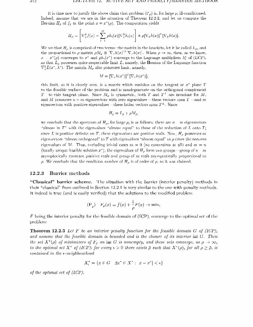
312 LECTURE 12. ACTIVE SET AND PENALTY/BARRIER METHODS
It is time now to justify the above claim that problem (P�) is, for large �, ill-conditioned.Indeed, assume that we are in the situation of Theorem 12.2.2, and let us compute theHessian H� of f� at the point x = x�(�). The computation yields
H� =
"r2xf(x) +
mXi=1
[�hi(x)]r2xhi(x)
#+ �[rxh(x)]
T [rxh(x)]:
We see that H� is comprised of two terms: the matrix in the brackets, let it be called L�, andthe proportional to � matrix �M� � [rxh(x)]T [rxh(x)]. When � ! 1, then, as we know,x = x�(�) converges to x� and �hi(x�) converge to the Lagrange multipliers ��i of (ECP),so that L� possesses quite respectable limit L, namely, the Hessian of the Lagrange functionr2xL(x
�; ��). The matrix M� also possesses limit, namely,
M = [rxh(x�)]T [rxh(x
�)];
this limit, as it is clearly seen, is a matrix which vanishes on the tangent at x� plane Tto the feasible surface of the problem and is nondegenerate on the orthogonal complementT? to this tangent plane. Since M� is symmetric, both T and T? are invariant for M ,and M possesses n �m eigenvectors with zero eigenvalues { these vectors span T { and meigenvectors with positive eigenvalues { these latter vectors span T?. Since
H� = L� + �M�;
we conclude that the spectrum of H�, for large �, is as follows: there are n�m eigenvectors
\almost in T" with the eigenvalues \almost equal" to those of the reduction of L onto T ;
since L is positive de�nite on T , these eigenvalues are positive reals. Now, H� possesses m
eigenvectors \almost orthogonal" to T with eigenvalues \almost equal" to � times the nonzero
eigenvalues of M . Thus, excluding trivial cases m = 0 (no constraints at all) and m = n
(locally unique feasible solution x�), the eigenvalues of H� form two groups { group of n�masymptotically constant positive reals and group of m reals asymptotically proportional to
�. We conclude that the condition number of H� is of order of �, as it was claimed.
12.2.3 Barrier methods
\Classical" barrier scheme. The situation with the barrier (interior penalty) methods intheir \classical" from outlined in Section 12.2.1 is very similar to the one with penalty methods.It indeed is true (and is easily veri�ed) that the solutions to the modi�ed problem
(P�) F�(x) � f(x) +1
�F (x)! min;
F being the interior penalty for the feasible domain of (ICP), converge to the optimal set of theproblem:
Theorem 12.2.3 Let F be an interior penalty function for the feasible domain G of (ICP),and assume that the feasible domain is bounded and is the closure of its interior int G. Thenthe set X�(�) of minimizers of F� on int G is nonempty, and these sets converge, as � ! 1,to the optimal set X� of (ICP): for every � > 0 there exists �� such that X�(�), for all � � ��, iscontained in the �-neighbourhood
X�� = fx 2 G j 9x� 2 X� : jx� x�j < �g
of the optimal set of (ICP).

12.2. PENALTY AND BARRIER METHODS 313
Proof is completely similar to that one of Theorem 12.2.1. First of all, X� is nonempty(since f is continuous and the feasible domain is bounded and closed and is therefore acompact set). The fact that X�(�) are nonempty for all positive � was proved in Section12.2.1. To prove that X�(�) is contained, for large �, in a tight neighbourhood of X�, let usact as follows. Same as in the proof of Theorem 12.2.1, it suÆces to lead to a contradictionthe assumption that there exists a sequence fxi 2 X�(�i)g with �i ! 1 which convergesto a point x 2 GnX�. Assume that it is the case; then f(x) > minG f + Æ with certainpositive Æ. Let x� be a global minimizer of f on G. Since G is the closure of int G, x� canbe approximated, within an arbitrarily high accuracy, by points from int G, and since f iscontinuous, we can �nd a point x0 2 int G such that
f(x0) � f(x�) +Æ
2:
We haveF�i(xi) = min
x2int GF�i (x) � F�i (x
0); (12.2.8)
whence
f(xi) +1
�iF (xi) � f(x0) +
1
�iF (x0):
Since F is a barrier for bounded domain G, F is below bounded on int G (since it attainsits minimum on int G { use the reasoning from Section 12.2.1 for the case of f � 0). Thus,F (x) � a > �1 for all x 2 int G, and therefore (12.2.8) implies that
f(xi) � f(x0) +1
�iF (x0)� 1
�ia:
As i ! 1, the right hand side in this inequality tends to f(x0) � f(x�) + Æ2 , and the left
hand side tends to f(x) � f(x�) + Æ; since Æ > 0, we get the desired contradiction.
If I were writing this lecture 5-8 years ago, I would proceed with the statements similar to theone of Theorem 12.2.2 and those on behaviour of the path of minimizers of F� and concludewith the same laments \all this is �ne, but the problems of minimization of F� normally (whenthe solution to the original problem is on the boundary of G; otherwise the problem actuallyis unconstrained) become the more ill-conditioned the larger is �, so that the diÆculties oftheir numerical solution grow with the penalty parameter". When indeed writing this lecture,I would say something quite opposite: there exists important situations when the diÆcultiesin numerical minimization of F� do not increase with the penalty parameter, and the overallscheme turns out to be theoretically eÆcient and, moreover, the best known so far. This changein evaluation of the scheme is the result of recent \interior point revolution" in Optimizationwhich I have already mentioned in Lecture 10. Those interested may get some impression ofessence of the matter from the below non-obligatory part of the lecture; please take into accountthat the prerequisite for reading it is non-obligatory Section 9.2.4 from Lecture 9.
Self-concordant barriers and path-following scheme
Assume from now on that our problem (ICP) is convex (the revolution we are speakingabout deals, at least directly, with Convex Programming only). It is well-known that convexprogram (ICP) can be easily rewritten as a program with linear objective; indeed, it suÆcesto extend the vector of design variables by one variable, let it be called t, more and to rewrite(ICP) as the problem
t! min j gj(x) � 0; j = 1; :::; k; f(x)� t � 0:

314 LECTURE 12. ACTIVE SET AND PENALTY/BARRIER METHODS
The resulting problem still is convex and has linear objective.To save notation, assume that the outlined conversion is carried out in advance, so that
already the original problem has linear objective and is therefore of the form
(P) f(x) � cTx! min j x 2 G � Rn:
Here the feasible set G of the problem is convex (we are speaking about convex programs!);we also assume that it is closed, bounded and possesses a nonempty interior.
Our abilities to solve (P) eÆciently by an interior point method depend on our abilitiesto point out a \good" interior penalty F for the feasible domain. What we are interested inis a #-self-concordant barrier F ; the meaning of these words is given by the following
De�nition 12.2.1 [Self-concordant barrier] Let # � 1. We say that a function F is #-self-concordant barrier for the feasible domain D of problem (P), if
� F is self-concordant function on int G (Section 9.2.4, Lecture 4), i.e., three timescontinuously di�erentiable convex function on int G possessing the barrier property(i.e., F (xi) ! 1 along every sequence of points xi 2 int G converging to a boundarypoint of G) and satisfying the di�erential inequality
j d3
dt3jt=0F (x+ th)j � 2
�hTF 00(x)h
�3=2 8x 2 int G 8h 2 Rn;
� F satis�es the di�erential inequality
jhTF 0(x)j �p#qhTF 00(x)h 8x 2 int G 8h 2 Rn: (12.2.9)
An immediate example is as follows (cf. \Raw materials" in Section 9.2.4, Lecture 4):
Example 12.2.1 [Logarithmic barrier for a polytope] Let
G = fx 2 Rn j aTj x � bj ; j = 1; :::;mgbe a polytope given by a list of linear inequalities satisfying the Slater condition (i.e., thereexists �x such that aTj �x < bj, j = 1; :::;m). Then the function
F (x) = �mXj=1
ln(bj � aTj x)
is an m-self-concordant barrier for G.
In the mean time, we shall justify this example (same as shall consider the crucial issue ofhow to �nd a self-concordant barrier for a given feasible domain). For the time being, let usfocus on another issue: how to solve (P), given a #-self-concordant barrier for the feasibledomain of the problem.
What we intend to do is to use the path-following scheme associated with the barrier {certain very natural implementation of the barrier method.
Path-following scheme
When speaking about the barrier scheme, we simply claimed that the minimizers of theaggregate F� approach, as � ! 1, the optimal set of (P). The immediate recommendationcoming from this claim could be: choose \large enough" value of the penalty and solve,for the chosen �, the problem (P�) of minimizing F�, thus coming to a good approximatesolution to (P). It makes, anyhow, sense to come to the solution of (P�) gradually, by solvingsequentially problems (P�i) along an increasing sequence of values of the penalty parameter.

12.2. PENALTY AND BARRIER METHODS 315
Namely, assume that the barrier F we use is nondegenerate, i.e., F 00(x) is positive de�nite atevery point x 2 int G (note that this indeed is the case when F is self-concordant barrier fora bounded feasible domain, see Proposition 9.2.2.(i)). Then the optimal set of F� for everypositive � is a singleton (we already know that it is nonempty, and the uniqueness of theminimizer follows from convexity and nondegeneracy of F�). Thus, we have a path
x�(�) = argminint G
F�(�);
as we know from Theorem 12.2.3, this path converges to the optimal set of (P) as � ! 1;besides this, it can be easily seen that the path is continuous (even continuously di�erentiable)in �. In order to approximate x�(�) with large values of � via the path-following scheme,we trace the path x�(�), namely, generate sequentially approximations x(�i) to the pointsx�(�t) along certain diverging to in�nity sequence �0 < �1 < ::: of values of the parameter.This is done as follows:
given \tight" approximation x(�t) to x�(�t), we update it into \tight" approximationx(�t+1) to x�(�t+1) as follows:
� �rst, choose somehow a new value �t+1 > �t of the penalty parameter
� second, apply to the function F�t+1 (�) a method for unconstrained minimization startedat x(�t), and run the method until closeness to the new target point x�(�t+1) is restored,thus coming to the new iterate x(�t+1) close to the new target point of the path.
All this is very close to what we did when tracing feasible surface with the GradientProjection scheme; our hope is that since x�(�) is continuous in � and x(�t) is \close" tox�(�t), for \not too large" �t+1��t the point x(�t) will be \not too far" from the new targetpoint x�(�t+1), so that the unconstrained minimization method we use will quickly restorecloseness to the new target point. With this \gradual" movement, we may hope to arrivenear x�(�) with large � faster than by attacking the problem (P�) directly.
All this was known for many years; and the progress during last decade was in trans-forming these qualitative ideas into exact quantitative recommendations.
Namely, it turned out that
� A. The best possibilities to carry this scheme out are when the barrier F is #-self-concordant; the less is the value of #, the better;
� B. The natural measure of \closeness" of a point x 2 int G to the point x�(�) of thepath is the Newton decrement of the self-concordant function
��(x) = �F�(x) � �cTx+ F (x)
at the point x, i.e., the quantity
�(��; x) =q[rx��(x)]T [r2
x��(x)]�1rx��(x)
(cf. Proposition 9.2.2.(iii)). More speci�cally, the notion \x is close to x�(�)" is conve-nient to de�ne as the relation
�(��; x) � 0:05 (12.2.10)
(in fact, 0.05 in the right hand side could be replaced with arbitrary absolute constant< 1, with slight modi�cation of subsequent statements; I choose this particular valuefor the sake of simplicity)
Now, what do all these words \the best possibility" and \natural measure" actually mean?It is said by the following two statements.

316 LECTURE 12. ACTIVE SET AND PENALTY/BARRIER METHODS
� C. Assume that x is close, in the sense of (12.2.10), to a point x�(�) of the path x�(�)associated with a #-self-concordant barrier for the feasible domain G of problem (P).Let us increase the parameter � to the larger value
�+ =
�1 +
0:08p#
�� (12.2.11)
and replace x by its damped Newton iterate (cf. (9.2.13), Lecture 4)
x+ = x� 1
1 + �(��+ ; x)[r2
x��+(x)]�1rx��+(x): (12.2.12)
Then x+ is close, in the sense of (12.2.10), to the new target point x�(�+) of the path.
C. says that we are able to trace the path (all the time staying close to it in the sense ofB.) increasing the penalty parameter linearly in the ratio (1+0:08#�1=2) and accompanyingeach step in the penalty parameter by a single Newton step in x. And why we should behappy with this, it is said by
� D. If x is close, in the sense of (12.2.10), to a point x�(�) of the path, then theinaccuracy, in terms of the objective, of the point x as of an approximate solution to(P) is bounded from above by 2#��1:
f(x)�minx2G
f(x) � 2#
�: (12.2.13)
D. says that the inaccuracy of the iterates x(�i) formed in the above path-followingprocedure goes to 0 as 1=�i, while C. says that we are able increase �i linearly, at the costof a single Newton step per each updating of �. Thus, we come to the following
Theorem 12.2.4 Assume that we are given
� (i) #-self-concordant barrier F for the feasible domain G of problem (P)
� (ii) starting pair (x0; �0) with �0 > 0 and x0 being close, in the sense of (12.2.10), tothe point x�(�0).
Consider the path-following method (cf. (12.2.11) - (12.2.12))
�t+1 =
�1 +
0:08p#
��t; xt+1 = xt � 1
1 + �(��t+1 ; xt)[r2
x��t+1(xt)]�1rx��t+1(xt):
(12.2.14)Then the iterates of the method are well-de�ned, belong to the interior of G and the methodpossesses linear global rate of convergence:
f(xt)�minG
f � 2#
�0
�1 +
0:08p#
��t: (12.2.15)
In particular, to make the residual in f less than a given � > 0, it suÆces to perform nomore that
N(�) �c20p# ln
�1 +
20#
�0�
�b (12.2.16)
Newton steps.
We see that the parameter # of the self-concordant barrier underlying the method is respon-sible for the Newton complexity of the method { the factor at the log-term in the complexitybound (12.2.16).

12.2. PENALTY AND BARRIER METHODS 317
Remark 12.2.3 The presented result does not explain how to start tracing the path { howto get initial pair (x0; �0) close to the path. This turns out to be a minor diÆculty: givenin advance a strictly feasible solution �x to (P), we could use the same path-following scheme(applied to certain arti�cial objective) to come close to the path x�(�), thus arriving at aposition from which we can start tracing the path. In our very brief outline of the topic, itmakes no sense to go in these \ details of initialization"; it suÆces to say that the necessity tostart from approaching x�(�) basically does not violate the overall complexity of the method.
It makes sense if not to prove the aforementioned statements { the complete proofs,although rather simple, go beyond the scope of our today lecture { but at least to motivatethem { to explain what is the role of self-concordance and \magic inequality" (12.2.9) inensuring properties C. and D. (this is all we need { the Theorem, of course, is an immediateconsequence of these two properties).
Let us start with C. { this property is much more important. Thus, assume we are at apoint x close, in the sense of (12.2.10), to x�(�). What this inequality actually says?
Let us denote byk h kH�1= (hTH�1h)1=2
the scaled Euclidean norm given by the inverse to the Hessian matrix
H � r2x��(x) = r2
xF (x)
(the equality comes from the fact that �� and F di�er by a linear function �f(x) � �cTx).Note that by de�nition of �(�; �) one has
�(�s; x) =k rx�s(x) kH�1�k sc+ F 0(x) kH�1 :
Due to the last formula, the closeness of x to x�(�) (see (12.2.10)) means exactly that
k rx��(x) kH�1�k �c+ F 0(x) kH�1� 0:05;
whence, by the triangle inequality,
k �c kH�1� 0:05+ k F 0(x) kH�1� 0:05 +p# (12.2.17)
(the concluding inequality here is given by (12.2.9) 8), and this is the main point where thiscomponent of the de�nition of a self-concordant barrier comes into the play).
From the indicated relations
�(��+ ; x) =k �+c+ F 0(x) kH�1�k (�+ � �)c kH�1 + k �c+ F 0(x) kH�1=
=j�+ � �
�k �c kH�1 +�(��; x) �
[see (12.2.11), (12.2.17)]
� 0:08p#(0:05 +
p#) + 0:05 � 0:134
(note that # � 1 by De�nition 12.2.1). According to Proposition 9.2.2.(iii.3), Lecture 4,the indicated inequality says that we are in the domain of quadratic convergence of thedamped Newton method as applied to self-concordant function ��+ ; namely, the indicatedProposition says that
�(��+ ; x+) � 2(0:134)2
1� 0:134< 0:05:
as claimed in C.. Note that this reasoning heavily exploits self-concordance of F
8)indeed, for a positive de�nite symmetric matrix H it clearly is the same (why?) to say that jgjH�1 � � andto say that jgThj � �jhjH for all h

318 LECTURE 12. ACTIVE SET AND PENALTY/BARRIER METHODS
To establish property D., it requires to analyze in more details the notion of a self-concordant barrier, and I am not going to do it here. Just to demonstrate where # comesfrom, let us prove an estimate similar to (12.2.13) for the particular case when, �rst, thebarrier in question is the standard logarithmic barrier given by Example 12.2.1 and, second,the point x is exactly the point x�(�) rather than is close to the latter point. Under theoutlined assumptions we have
x = x�(�)) rx��(x) = 0)
[substitute expressions for �� and F ]
�c+mXj=1
ajbj � aTj x
= 0)
[take inner product with x� x�, x� being an optimal solution to (P)]
�cT (x� x�) =mXj=1
aTj (x� � x)
bj � aTj x�
[take into account that aTj (x� � x) = aTj x
� � aTj x � bj � aTj x due to x� 2 G]
� m;
whence
cT (x� x�) � m
�� #
�
(for the case in question # = m). This estimate is twice better than (12.2.13) { this isbecause we have considered the case of x = x�(�) rather than the one of x close to x�(�).
Applications
The most famous (although, I believe, not the most important) application of Theorem 12.2.4deals with Linear Programming, when G is a polytope and F is the standard logarithmicbarrier for this polytope (see Example 12.2.1). For this case, the Newton complexity ofthe method9) is O(
pm), m being the # of linear inequalities involved into the description
of G. Each Newton step costs, as it is easily seen, O(mn2) arithmetic operations, so thatthe arithmetic cost per accuracy digit { number of arithmetic operations required to reducecurrent inaccuracy by absolute constant factor { turns out to be O(m1:5n2). Thus, we geta polynomial time solution method for LP, with complexity characteristics typically (for mand n of the same order) better than those for the Ellipsoid method (Lecture 7). Note alsothat with certain \smart" implementation of Linear Algebra, the above arithmetic cost canbe reduced to O(mn2); this is the best known so far cubic in the size of the problem uppercomplexity bound for Linear Programming.
To increase list of application examples, note that our abilities to solve in the outlinedstyle a convex program of a given structure are limited only by our abilities to point out self-concordant barrier for the corresponding feasible domain. In principle, there are no limitsat all { it can be proved that every closed convex domain in Rn admits a self-concordantbarrier with the value of parameter at most O(n). This \universal barrier" is given bycertain multivariate integral and is too complicated for actual computations; recall that we
9)recall that it is the factor at the logarithmic term in (12.2.16), i.e., the # of Newton steps suÆcient to reducecurrent inaccuracy by an absolute constant factor, say, by factor 2; cf. with the stories about polynomial timemethods from Lecture 7

12.2. PENALTY AND BARRIER METHODS 319
should form and solve Newton systems associated with our barrier, so that we need it to be\explicitly computable".
Thus, we come to the following important question:
How to construct \explicit" self-concordant barriers. There are many cases when weare clever enough to point out \explicitly computable self-concordant barriers" for convexdomains we are interested in. We already know one example of this type { Linear Program-ming (although we do not know to the moment why the standard logarithmic barrier fora polytope given by m linear constraints is m-self-concordant; why it is so, it will becomeclear in a moment). What helps us to construct self-concordant barriers and to evaluatetheir parameters are the following extremely simple combination rules, completely similar tothose for self-concordant functions (see Section 9.2.4, Lecture 4):
� [Linear combination with coeÆcients � 1] Let Fi, i = 1; :::m, be #i-self-concordantbarriers for the closed convex domains Gi, let the intersection G of these domainspossess a nonempty interior Q, and let �i � 1, i = 1; :::;m, be given reals. Then thefunction
F (x) =mXi=1
�iFi(x)
is (Pm
i=1 �i#i)-self-concordant barrier for G.
� [AÆne substitution] Let F (x) be #-self-concordant barrier for the closed convex domainG � Rn, and let x = A� + b be an aÆne mapping from Rk into Rn with the imageintersecting int G. Then the composite function
F+(�) = F (A� + b)
is #-self-concordant barrier for the closed convex domain
G+ = f� j A� + b 2 Ggwhich is the inverse image of G under the aÆne mapping in question.
The indicated combination rules can be applied to the \raw materials" as follows:
� [Logarithm] The function� ln(x)
is 1-self-concordant barrier for the nonnegative ray R+ = fx 2 R j x > 0g;[the indicated property of logarithm is given by 1-line computation]
� [Extension of the previous example: Logarithmic barrier, linear/quadratic case] Let
G = clfx 2 Rn j �j(x) < 0; j = 1; :::;mgbe a nonempty set in Rn given by m convex quadratic (e.g., linear) inequalities satis-fying the Slater condition. Then the function
f(x) = �mXi=1
ln(��i(x))
is m-self-concordant barrier for G.
[for the case when all the functions fi are linear, the conclusion immediately follows fromthe Combination rules (a polyhedral set given by m linear inequalities is intersection of mhalf-spaces, and a half-space is inverse image of the nonnegative axis under aÆne mapping;applying the combination rules to the barrier � lnx for the nonnegative ray, we get, withoutany computations, that the standard logarithmic barrier is for a polyhedral set is m-self-concordant). For the case when there are also quadratic forms among fi, you need a 1-2

320 LECTURE 12. ACTIVE SET AND PENALTY/BARRIER METHODS
lines of computations. Note that the case of linear fi covers the entire Linear Programming,while the case of convex quadratic fi covers much wider family of quadratically constrainedconvex quadratic problems.]
� The functionF (t; x) = � ln(t2 � xTx)
is 2-self-concordant barrier for the \ice-cream cone"
Kn+ = f(t; x) 2 R�Rn j t � jxjg;
the functionF (X) = � lnDet X
is n-self-concordant barrier for the cone Sn+ of positive de�nite symmetric n�nmatrices.One hardly could imagine how wide is the class of applications { from Combinatorial op-timization to Structural Design and Stability Analysis/Synthesis in Control { of the lattertwo barriers, especially of the lnDet -one.
Concluding remarks
The path-following scheme results in the most eÆcient, in terms of the worst-case complexityanalysis, interior point methods for Linear and Convex Programming. From the practicalviewpoint, anyhow, this scheme, in its aforementioned form, looks bad. The severe practicaldrawback of the scheme is its \short-step nature" { according to the scheme, the penaltyparameter should be updated by the \programmed" rule (12.2.11), and this makes the actualperformance of the method more or less close to the one given by (12.2.16). Thus, inthe straightforward implementation of the scheme the complexity estimate (12.2.16) willbe not just the theoretical upper bound on the worst-case complexity of the method, but theindication of the \typical" performance of the algorithm. And a method actually workingaccording to the complexity estimate (12.2.16) could be �ne theoretically, but it de�nitelywill be of very restricted practical interest in the large-scale case. E.g., in LP program withm � 105 inequality constraints and n � 104 variables (these are respectable, but in no sense\outstanding" sizes for a practical LP program) estimate (12.2.16) predicts something likehundreds of Newton steps with Newton systems of the size 104�104; even in the case of goodsparsity structure of the systems, such a computation would be much more time consumingthan the one given by the Simplex Method.
In order to get \practical" path-following methods, we need a long-step tactics { rulesfor on-line adjusting the stepsizes in the penalty parameter to, let me say, local curvatureof the path, rules which allow to update parameter as fast as possible { possible from theviewpoint of the actual \numerical circumstances" the method is in rather than from theviewpoint of very conservative theoretical worst-case complexity analysis.
Today there are eÆcient \long-step" policies of tracing the paths, policies which areboth �ne theoretically (i.e., satisfy complexity bound (12.2.16)) and very eÆcient computa-tionally. Extremely surprising phenomenon here is that for \good" long-step path-followingmethods as applied to convex problems of the most important classes (Linear Programming,Quadratically Constrained Convex Quadratic Programming and some other) it turns outthat
the actually observed number of Newton iterations required to solve the prob-lem within reasonable accuracy is basically independent of the sizes of the problemand is within 30-50.
This \empirical fact" (which can be only partly supported by theoretical considerations, notproved completely) is extremely important for applications; it makes polynomial time interiorpoint methods the most attractive (and sometimes - the only appropriate) optimization toolin many important large-scale applications.

12.2. PENALTY AND BARRIER METHODS 321
I should add that the eÆcient \long-step" implementations of the path-following schemeare relatively new, and for a long time10) the only interior point methods which demonstratedthe outlined \data- and size-independent" convergence rate were the so called potential re-duction interior point methods. In fact, the very �rst interior point method { the methodof Karmarkar for LP { which initialized the entire interior point revolution, was a potentialreduction algorithm, and what indeed caused the revolution was outstanding practical per-formance of this method. The method of Karmarkar possesses a very nice (and in fact verysimple) geometry and is closely related to the interior penalty scheme; anyhow, time limita-tions enforce me to skip description of this wonderful, although now a little bit old-fashioned,algorithm.
The concluding remark I would like to do is as follows: all polynomial time implemen-
tations of the penalty/barrier scheme known so far are those of the barrier scheme (which
is re ected in the name of these implementations: \interior point methods"); numerous at-
tempts to do something similar with the penalty approach failed to be successful. It is a
pity, due to some attractive properties of the scheme (e.g., here you do not meet with the
problem of �nding a feasible starting point, which, of course, is needed to start the barrier
scheme).
10)if I could qualify as \long" a part of the story which { the entire story { started in 1984