Technion - Israel Institute of Technology 1

On Interpolation Methods using

Statistical Models

RONEN SHER

Supervisor: MOSHE PORAT

2

Outline

Black & White image interpolation Motivations Concepts Flow Results

1D Signal interpolation CCD Demosaicing

Structure Methods Overview Components correlation Statistical extension Results

Summary

3

The Interpolation Problem

Factor of 2

11p 13p

22p21p

12p

33p

23p

32p31p

11p 12p 13p

31p

21p 22p 23p

32p 33pInput

Output

4

Image Interpolation Methods

i ii

p n

41

1 2 3 4 41

, i ii

p n

1n

p

4n 3n

2n

Nearest Neighbor

Bilinear

Bi-Cubic Spline

1 p n

163

1

, ( , )i i ii

p n f x y

5

Motivations 1: Pixels Correlation Normalized histograms of Lena (gray Levels)

256x256-dashed ; 512x512-solid

0 50 100 150 200 2500

0.01

0.02

0.03

His

togr

ams

512256

0 50 100 150 200 2500

0.2

0.4

0.6

0.8

1x 10

-6

Err

or

Gray Level

MSE=8.8461e-006

6

Motivations 2: Image Compression Results

Compression rates in bits/sample

3.50 : 43.75%81.33: 16.25% 25%8

“Necessary Data”:

7

Proposed Approach

,min | , , odd ,s i j sI I I I i j hist I hist I ,min | , , odds i jI I I I i j

min I I

3,min | , , odd , , 4s i j s cmpI I I I i j hist I hist I G

11p 12p 13p

31p

21p 22p 23p

32p 33p

8

Proposed Approach

M MI Near Lossless Compression

Scheme

2 2M MI

M MI Inverse Scheme 2 2M MI

9

Lossless Compression predictors

3 2 1p n n n 3n2n

p1n

4n1n

p2n 3n

2 4 1 2 4

2 4 1 2 4

2 4 1

min( , ) if max( , )

max( , ) if min( , )

otherwiseMED

MED

n n n n n

p n n n n n

n n n

p p

n p

p n

10

Lossless Compression - Context modeling

The error value is subtracted from the average error in a given context

3C

4n1n

p2n 3n 3 2 2 1 1 4, ,Q n n n n n n

1 2 3| , ,ie C C C

Vertical edgeHorizontal edge

1C2C

11

Outline

Black & White image interpolation Motivations Concepts Flow Results

1D Signal interpolation CCD Demosaicing

Structure Methods Overview Components correlation Statistical extension Results

Summary

12

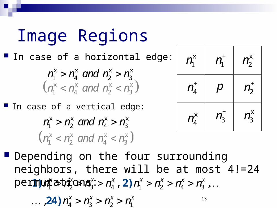
Image Regions

In regions of edges, averaging will result in a smoothing effect.

The edge must be preserved. The edges exist in the input image

and the same distribution is assumed in the larger interpolated image.

13

Image Regions In case of a horizontal edge:

x x x x1 4 2 3 n n and n n

x1n

p

+1n

x4n

x3n

x2n

+3n

+2n+

4n x x x x1 4 2 3 n n and n n

x x x x1 2 4 3 n n and n n

x x x x1 2 4 3 n n and n n

In case of a vertical edge:

1 2 3 4 1 2 4 3

4 3 2 1

, ,

,

x x x x x x x x

x x x x

n n n n n n n n

n n n n

1) 2)

4

2 )

Depending on the four surrounding neighbors, there will be at most 4!=24 permutations:

14

Pixels fitting

50 100 150 200 2500

50

100

150

200

nx1

p

Case8

50 100 150 200 2500

50

100

150

200

nx2

p

0 50 100 150 2000

50

100

150

200

nx3

p

0 100 200 3000

50

100

150

200

nx4

p

1n

p

4n 3n

2n

From Lena 256x256

15

Image Regions In each region a different weighted

sum is valid for the prediction4

x x x

1

i ii

p nx1n

p

+1n

x4n x

3n

x2n

+3n

+2n+

4n4

1

i ii

p n

The coefficients

are learned from the input image

24

1

+jα

j 24

1

xjα

j

16

Outline

Black & White image interpolation Motivations Concepts Flow Results

1D Signal interpolation CCD Demosaicing

Structure Methods Overveiw Components correlation Statistical extension Results

Summary

17

Step 1: Coefficients calculation Scanning the Input Image

for the ‘x type’ pixel we determine its permutation from its four neighbors and save its value and its neighbors’ values in VMx

Modeling only the regions with significant changes

in gray levels

Similar technique for the ‘+type’ pixels

x1n

p

+1n

x4n x

3n

x2n

+3n

+2n+

4n

4x

1i iV Var n Th

18

Step 1: Coefficients calculation For each permutation we find the four

coefficients using the Least Square solution:

4x x x

1

i ii

p n

1 11 12 13 14 1

2 21 22 23 24 2

3

1 2 3 4 4Q Q Q Q Q

p n n n n

p n n n n

p n n n n

Similar technique for the + coefficients

x1n

p

+1n

x4n x

3n

x2n

+3n

+2n+

4n

x xP nα1x xT T

α n n n P

19

Step 2a: ‘x type’ Reconstruction Scanning the sparse

Image, for each pixel we determine its matchingpermutation (coefficients)from its four neighbors and predict its valueusing 4

x x x

1

i ii

p n

11n 12n

? ?

13n

? ?

31n

21n 22n 23n

32n 33n

20

Step 2b: ‘+ type’ Reconstruction The Input is Ix,

for each “+” pixel we find its matching permutation (coefficients) and calculate its prediction by

11n 12n 13n

31n

21n 22n 23n

32n 33n

?

?

?

?

?

?

?

?

?

?

?x1P

x3P x

4P

x2P

?

4

1

i ii

p n

21

Experiments - Lena The 4 coefficients in 24 cases of x-type

Lena size 512x512

o Lena size 256x256

0 5 10 15 20 25-0.2

0

0.2

0.4

0.6

0.8

0 5 10 15 20 25

-0.2

0

0.2

0.4

0.6

0.8

0 5 10 15 20 25-0.2

0

0.2

0.4

0.6

0.8

0 5 10 15 20 25

-0.2

0

0.2

0.4

0.6

0.8

0 5 10 15 20 250

0.02

0.04

0.06

0.08

0.1

0.12

0.14

case

1, MSE=0.13652, MSE=0.0811773, MSE=0.181724, MSE=0.27006

Errors

α1

α4α3

α2

22

Example 1 - B&W images (128x128->256x256)Original Bilinear

Bi-Cubic Spline

Proposed Bi-Cubic

Nearest neighbor (Input)

23

Example 2 - B&W images (128x128->256x256)

Original Bilinear

Bi-Cubic Spline

Bi-Cubic

Nearest neighbor (Input)

Proposed

24

Outline

Black and White image interpolation Motivations Concepts Flow Results

1D Signal interpolation CCD Demosaicing

Structure Methods Overveiw Components correlation Statistical extension Results

Summary

25

One-Dimensional Interpolation

L L LPF

yin yd yd yrProcessing

DecimationInterpolation

k

ydyin

Interpolating yd, using NR. Its adjacent samples serve as the four neighbors for the coefficients’ calculation.

2L

26

Synthetic Test Signal

y1=sin(r.*(5+3.*sin(2.*(r+0.7)))).*sin(7.*(r+0.9)) t1=1,2..N1 r=(t1+OS1)/100 N1=2400 f1=1 Ts=2 OS1=3000 L=2

0 500 1000 1500 2000 2500 3000 3500 4000 4500 5000-1

-0.5

0

0.5

1

0 20 40 60 80 100 120 140 160 180 200

-0.5

0

0.5

1

Samples

yinyd

27

1D Interpolation result 1

3810 3820 3830 3840 3850 3860 3870 3880

-0.5

0

0.5

1

1.5S

igna

lsy

iny

Scy

NR

0 500 1000 1500 2000 2500 3000 3500 4000 4500 50000

1

2

3

4

5

Samples

Err

ors

ErrSc=1372.2358ErrNR=592.4323

28

1D Interpolation result 2

Voice signal: the word “Diskette”

29

Outline

Black and White image interpolation Motivations Concepts Flow Results

1D Signal interpolation CCD Demosaicing

Structure Methods Overveiw Components correlation Statistical extension Results

Summary

30

CCD structure

12R 14R

32R 34R

52R 54R 56R36R16R 11G

31G 35G33G15G13G

51G 53G 55G44G42G

22G 24G

62G 64G

26G

46G

66G

21B 23B 25B

43B 45B

61B 63B 65B41B

11G

44G42G31G 35G33G

15G13G

22G 24G

51G 53G 55G

12R 14R

32R 34R

52R 54R

62G 64G

26G

46G

66G56R

36R

16R

21B 23B 25B

41B 43B 45B

61B 63B 65B

31

CCD Demosaicing Methods

Bilinear Kimmel - gradient based function and

hues R/G,B/G. Gunturk – data consistency and similarity

between the high-frequency components. Muresan - interpolates R-G,B-G.

Not Linear Changing the Input

32

Basic Method

Treating each color component as an individual B&W image

Original Bilinear Proposed

33

Basic Method – Aliasing Effect

Original Bilinear Basic Method

34

Components method

Using all colors neighbors for the green reconstruction.

Reconstructing the difference of the colors components – Hues (R-G, B-G, R-B). Processing smoother signals.

35

Statistical generalization

Separating each case to sub-regions for better characterization.

Using the mean and the standard deviation of each neighbors’ set for the division (size invariant).

Each Sub-region will have its own coefficients – better representation of the region.

36

Case Study

RG R G

Case 1 2 3 4 5 6 7 8 9 10 11 12 13 14

Occurrence 1557 1145 889 1100 817 956 1182 897 1011 1158 920 770 1093 840

Coefficient Value

α1 0.18086α2 0.29814α3 0.32892α4 0.05548

Maximal Size Region:

From Light-House

37

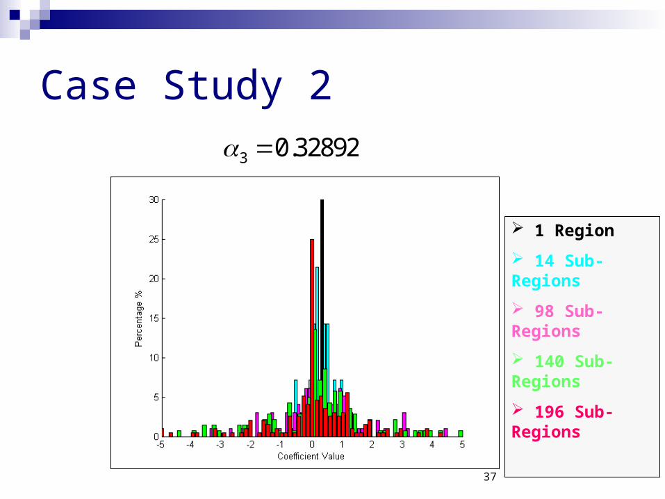
Case Study 2

1 Region

14 Sub-Regions

98 Sub-Regions

140 Sub-Regions

196 Sub-Regions

3 0.32892

38

Results 1 (384x256)Original Bi-Linear Gunturk

Optimal recovery Kimmel Neighbors Rule

Optimal Numeric Values:

σ – 2 divisions

E – 7 divisions

39

Results 2 (384x256)Original Bi-Linear Gunturk

Optimal recovery Kimmel Neighbors Rule

40

Summary A new interpolation method has been introduced

for 1D signals, B&W images and CCD color demosaicing based on the correlation between low and high resolution versions of a signal.

A non linear localized method has been developed to overcome the artificial effects caused by under-sampling.

The proposed method outperforms traditional methods in terms of MSE and visual perception.

Good results have been achieved in 2D interpolation and CCD demosaicing.

41

Appendix

42

Comparison: Basic vs. Components

43

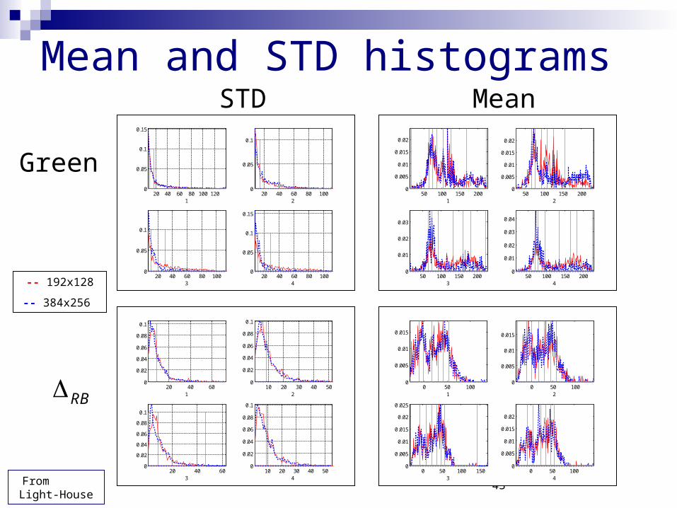
Mean and STD histograms

20 40 60 80 100 1200

0.05

0.1

0.15

120 40 60 80 100

0

0.05

0.1

2

20 40 60 80 1000

0.05

0.1

320 40 60 80 100

0

0.05

0.1

0.15

4

50 100 150 2000

0.005

0.01

0.015

0.02

150 100 150 200

0

0.005

0.01

0.015

0.02

2

50 100 150 2000

0.01

0.02

0.03

350 100 150 200

0

0.01

0.02

0.03

0.04

4

Mean

20 40 600

0.02

0.04

0.06

0.08

0.1

110 20 30 40 50

0

0.02

0.04

0.06

0.08

0.1

2

20 40 600

0.02

0.04

0.06

0.08

0.1

310 20 30 40 50

0

0.02

0.04

0.06

0.08

0.1

4

0 50 1000

0.005

0.01

0.015

10 50 100

0

0.005

0.01

0.015

2

0 50 100 1500

0.005

0.01

0.015

0.02

0.025

30 50 100

0

0.005

0.01

0.015

0.02

4

STD

Green

RB

-- 192x128

-- 384x256

From Light-House