technical specifications - pci geomatics · s technical specifications ` 3 beginner – module 1e...

Technical Specifications

1

s Technical Specifications `

2

Beginner – Module 1E

Contents

INTRODUCTION .............................................................................................................3

ABOUT THIS LAB ............................................................................................................3

IMPORTANCE OF THE MODULE .....................................................................................3

PRINCIPAL COMPONENT ANALYSIS ...............................................................................4

SCALING IMAGERY .........................................................................................................8

PERFORMING IMAGE FUSION ...................................................................................... 10

PAN SHARPENING IMAGERY ........................................................................................ 13

TOPICS LEARNED ......................................................................................................... 16

FURTHER READINGS .................................................................................................... 16

REFERENCES................................................................................................................. 16


3


Introduction Welcome to the Image Processing module, an introductory lab using

Geomatica’s Focus technology. This course lab is written for beginner users of

the geospatial software. In this lab you will master the basics needed to process

remote sensing imagery. This manual contains four modules. Each module

contains lessons that are built on basic tasks that you are likely to perform in

your daily work. They provide instruction for using the software to carry out

essential processes in Geomatica Focus.

About this Lab The following modules will be covered in this lab:

• Principal component analysis

• Scaling imagery

• Performing image fusion

• Pansharpening imagery

Each module in this course lab contains a series of hands-on lessons that let you work with the software and a set of sample data. Lessons have brief introductions followed by tasks and procedures in numbered steps. In addition, on the left panel, remote sensing theory in red font color and software tips in black font color can be found.

Importance of the Module There is an increasing amount of Remote Sensing data that is utilized in a

variety of applications. Image processing techniques allow to better capture

the essential information of the imagery. For this reason, it is fundamental to

understand how different image algorithms, such as image fusion and Principal

Component Analysis can be used to process data.

This module teaches the user how to use a variety of Geomatica processing

techniques with remote sensing imagery.


4


Principal component analysis

1. To start a new project from the File menu, select New Project. A window opens asking if you would like to save project changes.

2. Click No. A new project opens.

3 To open the PCA algorithm from the GEO Data folder, open

irvine.pix.

4 From the Tools menu> Algorithm Librarian> Image Processing folder (note 1).

5. Expand the Image Processing folder. A subcategory of folders appears.

6. In the Image Processing category, expand the Image Transformations folder.

A list of algorithms is displayed.

Note 1: The Algorithm Librarian window lets you access algorithms in the Algorithm Library. Algorithms are organized by themes or categories into a directory tree. You can expand a category in the tree to reveal sub-folders and algorithms.

Each algorithm in the Algorithm

Library has a Module Control Panel

(MCP) that you can open from the

Algorithm Librarian window.

Principal component analysis is a

linear transformation that rotates the axes of image space along lines of maximum variance. The rotation is based on the orthogonal eigenvectors of the covariance matrix generated from a sample of image data from the input channels. The output from this transformation is a new set of image channels, which are sometimes referred to as Eigen channels or principal components.

The first Eigen channel contains the

most variance in the dataset. The

second Eigen channel accounts for

additional variance in the dataset, but

is uncorrelated to the first. The third

Eigen channel accounts for the

remaining variance not accounted for

by the first two Eigen channels and is

uncorrelated with either of them. This

process continues until all the

variance in the dataset is accounted

for

Figure 1.0 Algorithm Librarian


5


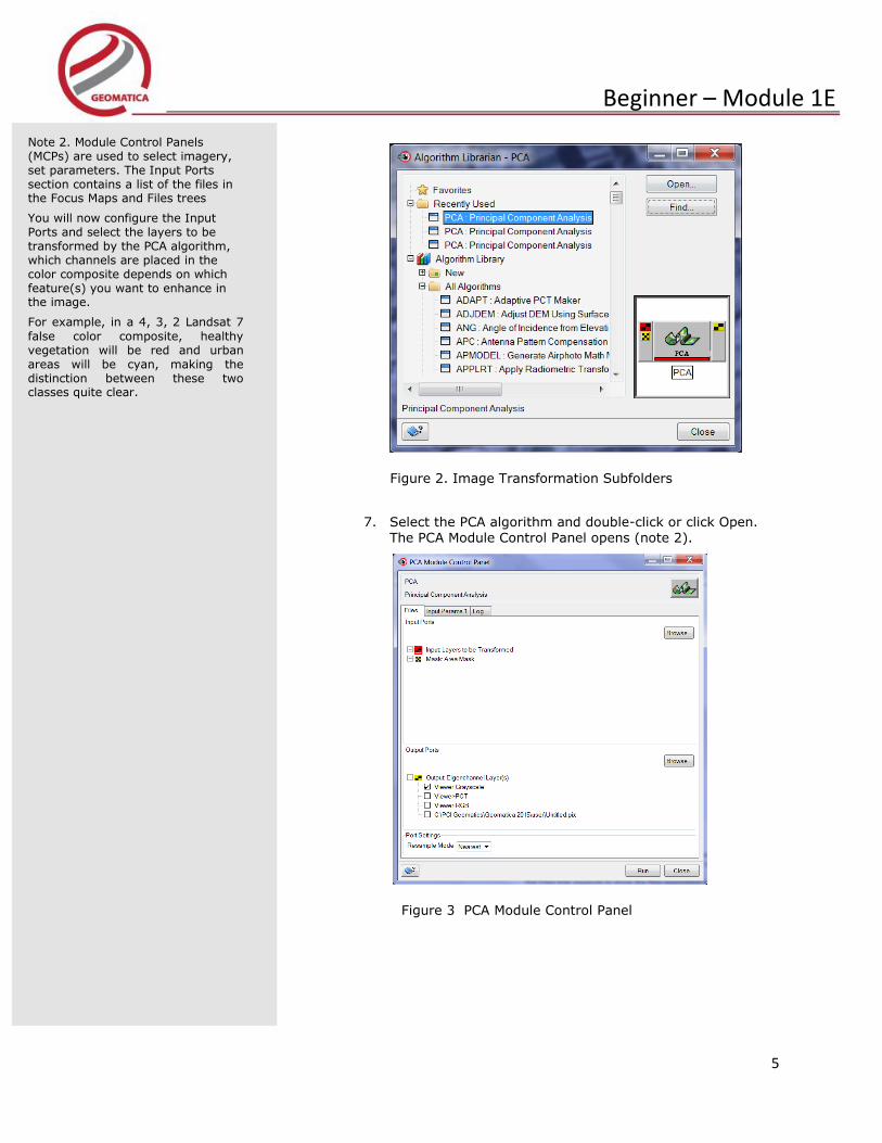
7. Select the PCA algorithm and double-click or click Open. The PCA Module Control Panel opens (note 2).

Note 2. Module Control Panels (MCPs) are used to select imagery, set parameters. The Input Ports section contains a list of the files in the Focus Maps and Files trees

You will now configure the Input Ports and select the layers to be transformed by the PCA algorithm, which channels are placed in the color composite depends on which feature(s) you want to enhance in the image.

For example, in a 4, 3, 2 Landsat 7

false color composite, healthy vegetation will be red and urban areas will be cyan, making the distinction between these two classes quite clear.

Figure 2. Image Transformation Subfolders

Figure 3 PCA Module Control Panel


6


8. To select the layers to be performed, in the Input Ports section, expand the Layers to be Transformed input port.

9. Expand the Files tree. The Files tree expands to show the files associated with your project.

10. Expand the irvine.pix file. The list expands to show the available raster layers in the file.

11. Select the check boxes beside TM bands 1 to 5.

Check marks appear in each box; and the input node for the Layers to be Transformed turns green.

12. In order to configure the output ports, make sure the Viewer-Grayscale is default in the Output Ports section

(note 3).

Need to examine the Eigen channels before you running the PCA algorithm to calculate:

13. To set the input parameters and calculate PCA, enter the input values in the parameters section and Click the Input Params 1 tab.

14. For the Eigen channels Layer Numbers, enter 1,2,3,4,5. This will calculate the eigenvectors for all five input channels.

15. For the Output Raster Type, select 8U.

16. For the Report Type, select SHORT.

Click Run (note 4).

Note 3: To configure the Output Ports

In the Output Ports section, make sure

the Viewer-Grayscale option is selected.

By specifying the Viewer as the output

option, the resulting channels of data are

not saved to a file; they are stored in

memory. This allows you to test

algorithms with different parameters and

only save the desired output.

By visually examining the Eigen channel

layers displayed > most of the variance

is contained within the first three Eigen

channels.

Now you will perform the actual transformation and output the first three Eigen channels to a new file.

Note 4. A progress Monitor opens on

your desktop. When the algorithm has finished executing, the Eigen channels are displayed in the Focus view area and the report is displayed in the Log tab of the MCP.

By visually examining the Eigen channel layers displayed in the view area and by examining the information in the report, you can see that most of the variance is contained within the first three Eigen channels. Now you will perform the actual transformation and output the first three Eigen channels to a new file.

Figure 4. Eigen channels 1, 2 and 3

displayed as a color composite in the view area


7


17. To configure the output ports, in the PCA MCP, click the Files tab.

18. In the Output Ports section, select both the Viewer-RGB option and the Untitled.pix option.

A check mark in each box.

19. Right-click the text box containing the path to the Untitled.pix file and select Browse.

20. Locate the GEO Data folder.

21. For the File name, type irvine_pca.pix and click Save. The path and file name are updated in the PCA Module Control Panel (note 5).

Before PCA transformation, you will set the input parameters.

22. In the PCA Module Control Panel, click the Input Params 1

tab.

23. For the Eigen channels Layer Numbers, enter 1,2,3. Only the first three Eigen channel layers will be retained for output.

24. For the Output Raster Type, select 8U.

25. For the Report Type, select LONG

26. For the Report Mode, select PCA.RPT.

27. Click Run (note 6).

.

Note 5: If a path for the output file is

not specified, the file is saved in the

user folder

Note 6: The Eigen channels are

created and saved to the output file

and the report is generated. Eigen

channels 1, 2 and 3 now contain 99%

of the variance from the original 5

input layers. You can also see a

“richer” dataset by displaying the

three Eigen channels as an RGB layer

Figure 5. Eigenchannels 1, 2 and 3 displayed as a color composite in the view area


8


Scaling Imagery

In this lesson you will on how to scale an image from 16 to 8 bit.

1. Start a New Project.

2. From the GEO Data folder, open radarsat.pix.

3. From the Tools menu, select Algorithm Librarian. The Algorithm Librarian window opens

4. Expand the Image Processing folder.

5. In the Image Processing category, expand the Image

Transformations folder.

A list of algorithms is displayed.

6. Select the SCALE algorithm and double-click or click Open. The SCALE Module Control Panel opens.

Remote sensing data is structured in 8-bit, 16-bit, and 32-bit formats.

For example, you can prepare data for visual display by scaling it from 16-bit or

32-bit to 8-bit. You can also scale data to a lower bit depth before you export it to applications that do not support data bits greater than 8.

For 8-bit data, the digital numbers (DN)

assigned to each pixel are between zero and 255. For 16-bit data, DNs can fall between zero and 65,535.We cannot visually benefit from images composed of thousands of shade variations.

SCALE can also be used to stretch or shift the dynamic range of an input image for visual enhancement. This Algorithm in the Library gives you control when scaling an image by allowing you to

specify your input minimum and maximum and your output minimum and maximum values.

Figure 5 Module Control Panel 1


9


7. To select the Unscaled Raster Layer(s), in the Input Ports section of the Files tab, expand the Unscaled Raster Layer(s) input port.

8. In the Files, expand the radarsat.pix file.

9. Select the check box beside the Standard 2 Beam Mode layer.

A check mark appears in the box and the Unscaled Raster Layer(s) input node turns green.

10. To configure the output ports, perform the same default steps and this time our file selection is going to be radarsat_scaled.pix and click Save (note 7).

11. In the SCALE Module Control Panel, click the Input Params 1 tab. Parameters specific to this algorithm are listed.

12. For the Minimum Input Gray Level Value, type 0.

13. For the Maximum Input Gray Level Value, type 30000.

This is the range of values used from the input channel(s).

The tail trimming option is grayed out when using these parameters.

14. For Scaling Function, select LIN.

15. For the Output Type, select 8 bit Unsigned.

16. Click Run (note 8).

Note 7: If a path for the output file is

not specified, the file is saved in the user

folder

Note 8: A Progress Monitor opens on

your desktop. When the algorithm has

finished executing, there is a message in

the Log tab indicating it scaled the input

values across the full range of values for

an 8-bit channel. The scaled image is

also displayed in the view area.

Figure 6 SCALE Module Control Panel


10


Performing image fusion

1. From the File menu, select Open. A File Selection window open.

2. Locate and open the GEO Data folder.

3. Hold down the Ctrl key and select toronto_qb_ms.pix and toronto_qb_pan.pix (note 9).

4. Click Open.

Both files are displayed in the view area and are listed in the Files tree.

5. To open the FUSE algorithm, go to Algorithm Librarian > Image Processing > Data Fusion Folder

6. Select the FUSE > The FUSE Module Control Panel opens

(note 10).

‘

.

7. To select the intensity layer, expand the Intensity Layer input port.

8. Select toronto_qb_pan.pix file.

The FUSE algorithm performs image

fusion of a Red-Green-Blue (RGB) color image with a black-and-white intensity image using the Intensity-Hue-Saturation (IHS) transformation.

The result is an output RGB color image

with the same resolution as the original black and white intensity image, but where the color (hue and saturation) is derived from the resampled input RGB image.

With the Intensity-Hue-Saturation

transformation image fusion technique, red, green and blue image channels are converted to intensity, hue and saturation image channels. The intensity channel is then substituted with the high resolution panchromatic image and the dataset is then converted back to the original RGB color space.

Note 9: The FUSE image fusion

algorithm has four input ports; the

Intensity Layer and the Red, Green and

Blue Layers. You will now configure the

Input Ports

Note 10. You will now access the Algorithm

Librarian to apply the FUSE algorithm to the

panchromatic and multispectral dataset from

Toronto, Ontario.

Figure 7. FUSE Module Control Panel


11


9. Select the check box beside the Panchromatic band. A check mark appears in the box and the Intensity Layer

input node turns green.

10. Collapse the Intensity Layer input port.

The FUSE image fusion algorithm has four input ports; the

Intensity Layer and the Red, Green and Blue Layers. You will now configure the Input Ports.

11. Expand the Red Layer > Files tree.

12. Expand the toronto_qb_ms.pix file.

13. Check box beside Band 3.

A check mark appears in the box and the Red Layer input

node turns green.

14. Expand the Green Layer

15. Select toronto_qb_ms.pix file with Band 2

16. To select the Blue Layer

17. Select toronto_qb_ms.pix file for Band 1

18. To configure the output ports, make sure the Viewer-RGB option is selected In the Output Ports section

19. Select the Untitled.pix option. A check mark appears in the box.

20. Right-click the text box containing the path to the Untitled.pix file and select Browse


22. For the File name, type toronto_qb_fuse.pix and click Save.

The path and file name are updated in the FUSE Module Control Panel.

23. Finally, set the input FUSE parameters, by clicking the Input Params 1 tab.

24. For the Resample Mode, select Cubic.

25. This is the resampling method applied to the input RGB image.

26. For the IHS model, select Cylinder. This is the color model used to convert from RGB to IHS and from IHS back to RGB.

27. Click Run.


12


When visually comparing the fused image to the original images, it is important to display the same band combinations and to apply the same enhancement to all images. In order to change the band combination for the original data, follow the next steps

28. In the Maps tree, select the toronto_qb_ms.pix RGB layer.

This becomes the active layer. 29. From the Layer menu, select the RGB Mapper. 30. Change the band combination of the original toronto_qb_ms.pix

RGB layer so it displays channels 3, 2, 1 as RGB (note 11). 31. Apply the same enhancement to both the original RGB layer and

the fused RGB layer (note 12).

Figure 7. FUSE Module Control Panel

Note 11: When visually comparing the fused image to the original images, it is important to display the same band combinations and to apply the same enhancement to all images. Note 12: You can switch back and forth between the fused image and the original images for a visual comparison by

dragging the toronto_qb_fuse.pix file up and down in the Maps tree or by turning it on and off. Another way of comparing the images is by using the Visualization Tools. Along with visual comparison, it is often useful to compare the histograms of the fused image to the histograms of the original images. This gives you information about the spectral quality of the fused product.


13


Pan sharpening imagery

1. From the Algorithm Librarian, double-click PANSHARP. The PANSHARP Module Control Panel opens.

2. To select the input multispectral image channels, in the Input Ports section, expand the Input Multispectral Image Channels input port (note 13).


4. Select all four Bands of QuickBird data. A check mark appears in each box and the Input Multispectral

Image Channels input node turns green.

5. Collapse the Input Multispectral Image Channels input port.

6. To select the reference image channels, expand the Reference Image Channels input port.


8. Select all four Bands of QuickBird data. A check mark appears in each box.

9. Collapse the Reference Image Channels input port (note 14 -15).

PANSHARP applies the automatic

image fusion algorithm to fuse a high-resolution panchromatic image with a multispectral image, creating a high-resolution color image.

This technique is often referred to as

pan-sharpening. It is an approach based on least squares developed to best approximate the gray value relationship between the original multispectral, panchromatic and the fused images to achieve a best color representation.

The power of PANSHARP lies in the

simplicity of its algorithm and its versatility. It works with any image data type - 8-bit unsigned, 16-bit signed/unsigned, 32-bit floating point and is computationally efficient. It can also fuse images acquired simultaneously by the same sensor or use images from different sensors.

Note 13. The PANSHARP fusion algorithm has three input ports; the Input Multispectral Image Channels and the Panchromatic Image Channel, which are mandatory, and

the Reference Image Channels, which is an optional input. You will now configure the input ports. Note 14: The Reference Image

Channels must be specified unless

the multispectral and panchromatic

files contain wavelength metadata.

Note 15: The Reference Image

Channels span the same wavelength

response range as the panchromatic

image layer specified for the Input

Panchromatic Image input port. The

reference channels used vary from

sensor to sensor.

Figure 9. PANSHARP Module Control Panel


14


10. Expand the Panchromatic Image Channel input port.

11. Expand the toronto_qb_pan.pix file.

12. Select the Panchromatic Band. A check mark appears in the box.

13. Collapse the Panchromatic Image Channel input port.

14. To configure the output ports, make sure the Viewer-RGB option is selected in the Output Ports section

15. Select the Untitled.pix option. A check mark appears in the box.

16. Right-click the text box containing the path to the Untitled.pix file and select Browse.


18. For the File name, type toronto_qb_pansharp.pix and click Save.

19. The path and file name are updated in the PANSHARP Module Control Panel.

Figure 10. PANSHARP Module Control Panel Input Ports


15


Before you run the PANSHARP algorithm, you will set the input parameters.

20. To set the input parameters and run PANSHARP, go to Input

Params 1 tab.

21. For the Enhanced Pansharpening, select Yes. This applies a high-pass filter to enhance the visual results.

22. Click Run.

To change the band combination for the PANSHARP layer

23. In the Maps tree, select the toronto_qb_pansharp.pix RGB layer.

This becomes the active layer.

24. From the Layer menu, select the RGB Mapper (note 16 -17).

25. Change the band combination of the toronto_qb_pansharp.pix

RGB layer so it displays channels 3, 2, 1 as RGB.

26. Apply the same enhancement to all RGB layers (note 18).

Note 16: When visually comparing

the fused image to the original

images, it is important to display

the same band combinations and to

apply the same enhancement to all

images.

Note 17: You can switch back and

forth between the pansharpened

image and the original images for a

visual comparison by dragging the

toronto_qb_pansharp.pix file up and

down in the Maps tree or by turning

it on and off. Another way of

comparing the images is by using

the Visualization Tools.

Note 18: Along with visual

comparison, it is often useful to

compare the histograms of the

pansharpened image to the

histograms of the original images.

This gives you information about

the spectral quality of the

pansharpened product.


16


Topics Learned

Further Readings • Characteristics of Images

• Image Pre-processing

• PCA

• Image Transformations

• Pansharpening Data in Geomatica

References

Remote Sensing Theory • PCA • Image Fusion • Pansharpening • Image Scaling

Geomatica:

• Set up and performed Principal Component Analysis

• Image Scaling • Set up and performed image fusion

using the FUSE algorithm • Set up and ran the PANSHARP

algorithm

http://www.nrcan.gc.ca/earth-sciences/geomatics/satellite-imagery-air-photos/satellite-imagery-products/educational-resources/14641


http://fas.org/irp/imint/docs/rst/Sect1/Sect1_14.html


http://support.pcigeomatics.com/hc/en-us/articles/203482689-Pansharpening-Data-in-Geomatica-

technical specifications - pci geomatics · s technical specifications ` 3 beginner – module 1e...

Documents