technical reports series no. - iaea scientific and ... · technical reports series no.429. ... all...
TRANSCRIPT

Guidelines for Application of the Master Curve Approach to Reactor
Pressure Vessel Integrity in Nuclear Power Plants
Technical Reports SeriEs No. 429

GUIDELINES FOR APPLICATIONOF THE MASTER CURVE
APPROACH TO REACTORPRESSURE VESSEL INTEGRITYIN NUCLEAR POWER PLANTS

The following States are Members of the International Atomic Energy Agency:
AFGHANISTANALBANIAALGERIAANGOLAARGENTINAARMENIAAUSTRALIAAUSTRIAAZERBAIJANBANGLADESHBELARUSBELGIUMBENINBOLIVIABOSNIA AND HERZEGOVINABOTSWANABRAZILBULGARIABURKINA FASOCAMEROONCANADACENTRAL AFRICAN REPUBLICCHILECHINACOLOMBIACOSTA RICACÔTE D’IVOIRECROATIACUBACYPRUSCZECH REPUBLICDEMOCRATIC REPUBLIC OF THE CONGODENMARKDOMINICAN REPUBLICECUADOREGYPTEL SALVADORERITREAESTONIAETHIOPIAFINLANDFRANCEGABONGEORGIAGERMANYGHANAGREECE
GUATEMALAHAITIHOLY SEEHONDURASHUNGARYICELANDINDIAINDONESIAIRAN, ISLAMIC REPUBLIC OF IRAQIRELANDISRAELITALYJAMAICAJAPANJORDANKAZAKHSTANKENYAKOREA, REPUBLIC OFKUWAITKYRGYZSTANLATVIALEBANONLIBERIALIBYAN ARAB JAMAHIRIYALIECHTENSTEINLITHUANIALUXEMBOURGMADAGASCARMALAYSIAMALIMALTAMARSHALL ISLANDSMAURITANIAMAURITIUSMEXICOMONACOMONGOLIAMOROCCOMYANMARNAMIBIANETHERLANDSNEW ZEALANDNICARAGUANIGERNIGERIANORWAYPAKISTANPANAMA
PARAGUAYPERUPHILIPPINESPOLANDPORTUGALQATARREPUBLIC OF MOLDOVAROMANIARUSSIAN FEDERATIONSAUDI ARABIASENEGALSERBIA AND MONTENEGROSEYCHELLESSIERRA LEONESINGAPORESLOVAKIASLOVENIASOUTH AFRICASPAINSRI LANKASUDANSWEDENSWITZERLANDSYRIAN ARAB REPUBLICTAJIKISTANTHAILANDTHE FORMER YUGOSLAV REPUBLIC OF MACEDONIATUNISIATURKEYUGANDAUKRAINEUNITED ARAB EMIRATESUNITED KINGDOM OF GREAT BRITAIN AND NORTHERN IRELANDUNITED REPUBLIC OF TANZANIAUNITED STATES OF AMERICAURUGUAYUZBEKISTANVENEZUELAVIETNAMYEMENZAMBIAZIMBABWE
The Agency’s Statute was approved on 23 October 1956 by the Conference on the Statute othe IAEA held at United Nations Headquarters, New York; it entered into force on 29 July 1957The Headquarters of the Agency are situated in Vienna. Its principal objective is “to accelerate andenlarge the contribution of atomic energy to peace, health and prosperity throughout the world’’.
© IAEA, 2005
Permission to reproduce or translate the information contained in this publication may beobtained by writing to the International Atomic Energy Agency, Wagramer Strasse 5, P.O. Box 100A-1400 Vienna, Austria.
Printed by the IAEA in AustriaMarch 2005
STI/DOC/010/429
f .
,

TECHNICAL REPORTS SERIES No. 429
GUIDELINES FOR APPLICATIONOF THE MASTER CURVE
APPROACH TO REACTORPRESSURE VESSEL INTEGRITYIN NUCLEAR POWER PLANTS
INTERNATIONAL ATOMIC ENERGY AGENCYVIENNA, 2005

IAEA Library Cataloguing in Publication Data
Guidelines for application of the master curve approach to reactor pressure vessel integrity in nuclear power plants. — Vienna : International Atomic Energy Agency, 2005.
p. ; 24 cm. — (Technical reports series, ISSN 0074–1914 ; no. 429)STI/DOC/010/429ISBN 92–0–112104–0Includes bibliographical references.
1. Nuclear pressure vessels. 2. Nuclear power plants. I. International Atomic Energy Agency. II. Technical reports series (International Atomic Energy Agency) ; 429.
IAEAL 05–00397
COPYRIGHT NOTICE
All IAEA scientific and technical publications are protected by the terms of the Universal Copyright Convention as adopted in 1952 (Berne) and as revised in 1972 (Paris). The copyright has since been extended by the World Intellectual Property Organization (Geneva) to include electronic and virtual intellectual property. Permission to use whole or parts of texts contained in IAEA publications in printed or electronic form must be obtained and is usually subject to royalty agreements. Proposals for non-commercial reproductions and translations are welcomed and will be considered on a case by case basis. Enquiries should be addressed by email to the Publishing Section, IAEA, at [email protected] or by post to:
Sales and Promotion Unit, Publishing SectionInternational Atomic Energy AgencyWagramer Strasse 5P.O. Box 100A-1400 ViennaAustriafax: +43 1 2600 29302tel.: +43 1 2600 22417http://www.iaea.org/Publications/index.html

FOREWORD
The guidelines in this report have been developed under an IAEA Coordinated Research Project (CRP) entitled Surveillance Programme Results Application to Reactor Pressure Vessel Integrity Assessment. This CRP is the fifth in a series that have led to a focus being placed on the measurement of the best irradiated fracture toughness parameters using relatively small test specimens for ensuring the structural integrity of reactor pressure vessel (RPV) materials. These guidelines are intended to allow utility engineers and scientists to measure fracture toughness directly using small surveillance-sized specimens and to apply the results using the Master Curve approach for RPV structural integrity assessment in nuclear power plants.
The Master Curve approach for assessing the fracture toughness of a sampled irradiated material has been gaining acceptance throughout the world. This direct measurement approach is preferred to the indirect and correlative methods used in the past to assess irradiated RPV integrity. These other methods have used the Charpy V-notch transition temperature shift (usually defined at the 41J temperature, T41J) as the measure of radiation embrittlement. These methods, when combined with reference fracture toughness curves, such as the ASME code KIC and KIa (or KIR) curves, allow the determination of a lower bound linear elastic fracture toughness that has consistently been shown to be conservative relative to the measurement of actual fracture toughness.
Expertise in implementing results obtained from Master Curve testing was originally developed by K. Wallin of VTT, Finland. The Master Curve method of defining a single reference transition temperature, T0, has been standardized in ASTM Standard Test Method E 1921. There have been comparisons and applications made using Master Curve data in several countries, but the primary attempts at licensing implementation for nuclear reactor safety of RPV steels have been in the United States of America. The approach taken in the USA has been to focus on using the Master Curve to provide an alternative transition temperature index parameter to that of RTNDT. The benefit of this approach is that fracture toughness can be measured directly on irradiated sample materials rather than having to measure initial properties and add a Charpy V-notch transition temperature shift.
Special thanks are due to W.L. Server of ATI Consulting (USA) who chaired the meetings and M. Brumovský of the Nuclear Research Institute (Czech Republic) and S. Rosinski of the Electric Power Research Institute (USA) who also made significant contributions to the report. The IAEA officers responsible for the preparation of the report were V.N. Lyssakov and Ki-Sig Kang of the Division of Nuclear Power.

EDITORIAL NOTE
Although great care has been taken to maintain the accuracy of information contained in this publication, neither the IAEA nor its Member States assume any responsibility for consequences which may arise from its use.
The use of particular designations of countries or territories does not imply any judgement by the publisher, the IAEA, as to the legal status of such countries or territories, of their authorities and institutions or of the delimitation of their boundaries.
The mention of names of specific companies or products (whether or not indicated as registered) does not imply any intention to infringe proprietary rights, nor should it be construed as an endorsement or recommendation on the part of the IAEA.
The authors are responsible for having obtained the necessary permission for the IAEA to reproduce, translate or use material from sources already protected by copyrights.

CONTENTS
1. INTRODUCTION . . . . . . . . . . . . . . . . . . . . . . . . . . . . . . . . . . . . . . . . . 1
2. BACKGROUND . . . . . . . . . . . . . . . . . . . . . . . . . . . . . . . . . . . . . . . . . . 3
2.1. Sample material and testing in accordance with ASTM E 1921 42.2. Best estimate of T0 for sample material . . . . . . . . . . . . . . . . . . . 62.3. Best estimate of T0 for RPV limiting material . . . . . . . . . . . . . . 62.4. Fluence function and projection . . . . . . . . . . . . . . . . . . . . . . . . . 72.5. Application definition and key parameters . . . . . . . . . . . . . . . . 92.6. Deterministic evaluation . . . . . . . . . . . . . . . . . . . . . . . . . . . . . . . . 92.7. Probabilistic analysis . . . . . . . . . . . . . . . . . . . . . . . . . . . . . . . . . . . 10
3. MATERIAL AND APPLICATION ISSUES . . . . . . . . . . . . . . . . . . 11
3.1. Sample materials available . . . . . . . . . . . . . . . . . . . . . . . . . . . . . . 113.2. Fluence and transition temperature limits . . . . . . . . . . . . . . . . . 133.3. Application issues . . . . . . . . . . . . . . . . . . . . . . . . . . . . . . . . . . . . . 15
3.3.1. P–T curves . . . . . . . . . . . . . . . . . . . . . . . . . . . . . . . . . . . . . 153.3.2. PTS . . . . . . . . . . . . . . . . . . . . . . . . . . . . . . . . . . . . . . . . . . . 153.3.3. Transferability of toughness values . . . . . . . . . . . . . . . . . 163.3.4. Acceptability of defects found during
in-service inspection . . . . . . . . . . . . . . . . . . . . . . . . . . . . . 173.4. Master Curve approaches . . . . . . . . . . . . . . . . . . . . . . . . . . . . . . . 17
4. DETERMINATION OF T0 . . . . . . . . . . . . . . . . . . . . . . . . . . . . . . . . . 18
4.1. General evaluation procedure for T0 determination . . . . . . . . . 184.1.1. Fracture toughness evaluation . . . . . . . . . . . . . . . . . . . . . 184.1.2. Validity check . . . . . . . . . . . . . . . . . . . . . . . . . . . . . . . . . . 194.1.3. Prediction of size effects and transition temperature . . 194.1.4. Determination of T0 . . . . . . . . . . . . . . . . . . . . . . . . . . . . . 204.1.5. Establishment of the transition temperature curve
(Master Curve) and tolerance bounds . . . . . . . . . . . . . . 214.2. Sequence of T0 determination . . . . . . . . . . . . . . . . . . . . . . . . . . . 22
4.2.1. Selection of test temperatures and testing of specimens . . . . . . . . . . . . . . . . . . . . . . . . . . . . . . . . . . . . 22
4.2.2. Determination of T0 (ASTM E 1921) . . . . . . . . . . . . . . . 244.2.3. Checking the validity of T0 (ASTM E 1921-02) . . . . . . 24
4.3. Analysis of abnormal fracture toughness data . . . . . . . . . . . . . . 254.3.1. Inhomogeneous materials . . . . . . . . . . . . . . . . . . . . . . . . 264.3.2. Grain boundary fracture . . . . . . . . . . . . . . . . . . . . . . . . . 294.3.3. Extrapolation outside the standard validity window . . 30
4.4. Uncertainty in T0 and low bound curve for KJc . . . . . . . . . . . . . 31
5. DETERMINATION OF T0 FOR RPV MATERIAL . . . . . . . . . . . 32
5.1. Methodology to determine T0 for RPV material . . . . . . . . . . . . 325.2. Example application . . . . . . . . . . . . . . . . . . . . . . . . . . . . . . . . . . . 36
6. FLUENCE PROJECTION INCLUDING ATTENUATION . . . . 38
6.1. Introduction . . . . . . . . . . . . . . . . . . . . . . . . . . . . . . . . . . . . . . . . . . 386.2. Embrittlement trend curves . . . . . . . . . . . . . . . . . . . . . . . . . . . . . 396.3. Considerations for attenuation . . . . . . . . . . . . . . . . . . . . . . . . . . 426.4. Summary and recommendations . . . . . . . . . . . . . . . . . . . . . . . . . 48
7. DETERMINISTIC ANALYSIS AND METHODS . . . . . . . . . . . . . 49
7.1. Introduction . . . . . . . . . . . . . . . . . . . . . . . . . . . . . . . . . . . . . . . . . . 497.2. Application of the ASME Code Cases N-629 and N-631 . . . . . 517.3. Application of the Master Curve approach to
WWER type reactors . . . . . . . . . . . . . . . . . . . . . . . . . . . . . . . . . . 537.4. Generic values of RTT0 . . . . . . . . . . . . . . . . . . . . . . . . . . . . . . . . . 557.5. Evaluation of uncertainties . . . . . . . . . . . . . . . . . . . . . . . . . . . . . . 56
7.5.1. Shift method . . . . . . . . . . . . . . . . . . . . . . . . . . . . . . . . . . . 577.5.2. Direct method . . . . . . . . . . . . . . . . . . . . . . . . . . . . . . . . . . 58
7.6. Application of a Master Curve tolerance bound . . . . . . . . . . . . 597.7. Relationship between margin (Y) and tolerance bound (X) . . 637.8. Master Curve shape . . . . . . . . . . . . . . . . . . . . . . . . . . . . . . . . . . . . 65
8. PROBABILISTIC APPLICATION . . . . . . . . . . . . . . . . . . . . . . . . . . 67
8.1. Possible approaches . . . . . . . . . . . . . . . . . . . . . . . . . . . . . . . . . . . . 678.1.1. Flaws . . . . . . . . . . . . . . . . . . . . . . . . . . . . . . . . . . . . . . . . . . 678.1.2. Transients . . . . . . . . . . . . . . . . . . . . . . . . . . . . . . . . . . . . . . 688.1.3. Uncertainties in material toughness values . . . . . . . . . . 68
8.2. Probabilistic analysis . . . . . . . . . . . . . . . . . . . . . . . . . . . . . . . . . . . 69
9. CONCLUSION . . . . . . . . . . . . . . . . . . . . . . . . . . . . . . . . . . . . . . . . . . . . 73

APPENDIX I: SINTAP FRACTURE TOUGHNESS ESTIMATION: ANALYSIS OF DATA FOR INITIATION OF BRITTLE FRACTURE . . . . . . . . . . . . . . . . . . . . . . . 75
I.1. Overview . . . . . . . . . . . . . . . . . . . . . . . . . . . . . . . . . . . . . . . . . . . . . 75I.2. Preliminary steps . . . . . . . . . . . . . . . . . . . . . . . . . . . . . . . . . . . . . . 75I.3. SINTAP procedure . . . . . . . . . . . . . . . . . . . . . . . . . . . . . . . . . . . . 80
I.3.1. Stage 1: MML estimation of T0 . . . . . . . . . . . . . . . . . . . . 80I.3.2. Stage 2: Lower tail estimation . . . . . . . . . . . . . . . . . . . . . 80I.3.3. Stage 3: Minimum value estimation . . . . . . . . . . . . . . . . 81
I.4. Determination of characteristic values . . . . . . . . . . . . . . . . . . . . 81
APPENDIX II: EXAMPLES OF ABNORMAL FRACTURE TOUGHNESS DATA ASSESSMENT . . . . . . . . . . . . . . 83
II.1. Examples: SINTAP application . . . . . . . . . . . . . . . . . . . . . . . . . . 83II.2. Master Curve and grain boundary fracture . . . . . . . . . . . . . . . . 84II.3. Examples: Application of the Master Curve outside
the –50°C ≤ T – T0 ≤ +50°C range . . . . . . . . . . . . . . . . . . . . . . . . 87II.3.1. General principle . . . . . . . . . . . . . . . . . . . . . . . . . . . . . . . 87II.3.2. Application near the lower shelf . . . . . . . . . . . . . . . . . . . 87II.3.3. Application near the upper shelf . . . . . . . . . . . . . . . . . . . 87II.3.4. Lower shelf adjustment: Background . . . . . . . . . . . . . . . 88II.3.5. Lower shelf adjustment: Application . . . . . . . . . . . . . . . 89
APPENDIX III: PROMETEY PROBABILISTIC MODEL FOR FRACTURE TOUGHNESS PREDICTION . . . . . . . . 91
III.1. The local criterion for cleavage fracture . . . . . . . . . . . . . . . . . . . 92III.2. The probabilistic model for the KIC(T) curve prediction . . . . . 93III.3. Experimental determination of parameters necessary
for brittle fracture toughness prediction . . . . . . . . . . . . . . . . . . . 94
APPENDIX IV: LIST OF ABBREVIATIONS AND SYMBOLS. . . . . . 96
REFERENCES . . . . . . . . . . . . . . . . . . . . . . . . . . . . . . . . . . . . . . . . . . . . . . . . 99CONTRIBUTORS TO DRAFTING AND REVIEW . . . . . . . . . . . . . . . 105


1. INTRODUCTION
The guidelines in this report have been developed under an IAEA Coordinated Research Project (CRP) entitled Surveillance Programme Results Application to Reactor Pressure Vessel Integrity Assessment. The IAEA has sponsored a series of five CRPs that have led to a focus being placed on the measurement of the best irradiation fracture parameters using relatively small test specimens for ensuring structural integrity of reactor pressure vessel (RPV) materials in nuclear power plants. The background and results from the series of CRPs are described in the following paragraphs.
The first project (or phase 1), Irradiation Embrittlement of Reactor Pressure Vessel Steels, focused on the standardization of methods for measuring embrittlement both in terms of mechanical properties and the neutron irradiation environment. Little attention was given at that time (early 1970s) to the direct measurement of irradiated fracture toughness of small surveillance type specimens since elastic–plastic fracture mechanics was in its infancy. The main results from phase 1, including all reports from participating organizations, were published in 1975 [1].
Phase 2, Analysis of the Behaviour of Advanced Reactor Pressure Vessel Steels under Neutron Irradiation, involved testing and evaluation by various countries of so-called advanced RPV steels that had reduced residual compositional elements (copper and phosphorus). Irradiations were conducted to fluence levels beyond expected end-of-life (EOL), and the results of phase 1 were used to guide the overall approach taken during phase 2. In addition to transition temperature testing using Charpy V-notch test specimens, some emphasis was placed on using tensile and early design fracture toughness test specimens applying elastic–plastic fracture mechanics methods. Further progress in the application of fracture mechanics analysis methods to radiation damage assessment was achieved in this phase. Improvement and unification of neutron dosimetry methods provided better data with less inherent scatter. All results, together with their analyses and raw data, are summarized in Ref. [2].
Phase 3, Optimizing Reactor Pressure Vessel Surveillance Programmes and Their Analyses, included the direct measurement of fracture toughness using irradiated surveillance specimens. Significant results were achieved with regard to fracture toughness testing and structural integrity methods and correlations between various toughness and strength measures for irradiated materials, which emphasized the need to understand embrittlement mechanisms and the potential mitigation measures for radiation embrittlement. Key achievements were the acquisition and testing of a series of RPV steels designed and selected for radiation embrittlement research. One of
1
these materials was given the code JRQ, and it has been shown to be an excellent correlation monitor (or standard reference) material as documented in Ref. [3].
The main emphasis of the fourth phase, Assuring Structural Integrity of Reactor Pressure Vessels, which began in 1995, was on the experimental verification of the Master Curve approach for surveillance-sized specimens. This CRP was directed at confirmation of the measurement and interpretation of fracture toughness using the Master Curve method with structural integrity assessment of irradiated RPVs as the ultimate goal. The main conclusions from the phase 4 CRP are that the Master Curve approach has demonstrated that small-sized specimens, such as precracked Charpy, can be used to determine valid values of fracture toughness in the transition temperature region. Application included a large test matrix using the JRQ steel and other national steels, including WWER materials. No differences in laboratories were identified and results from dynamic data also followed the Master Curve.
Phase 5 (Surveillance Programme Results Application to Reactor Pressure Vessel Integrity Assessment) is nearing completion. The last meeting of the general CRP group was held in February 2003 and involved 20 testing laboratories representing 15 countries. This CRP has two main objectives:
(1) To develop a large database of fracture toughness data using the Master Curve methodology for both precracked Charpy-sized and one inch thick (25.4 mm) compact tension (1T-CT) specimens to assess possible specimen bias effects and any effects of the range of temperatures used to determine T0, either using the single temperature or multitemperature assessment methods.
(2) To develop international guidelines for measuring and applying Master Curve fracture toughness results for RPV integrity assessment.
Preliminary results show clear evidence that lower values of unirradiated T0 are obtained using precracked Charpy specimens, compared with results from 1T-CT specimens. This bias in test results is very important when considering the use of precracked Charpy specimens in evaluating RPV integrity.
This report provides guidelines for the application of the Master Curve approach for small surveillance-sized specimens. Scientists and engineers from the Czech Republic, the European Commission (Joint Research Centre), Finland, France, Germany, the Russian Federation, Spain and the United States of America contributed to the development of these guidelines. Concurrent with the development of these guidelines is the analysis of a large database of Master Curve fracture toughness data. The preliminary evaluation
2
results have helped to define the general ‘road map’ for the IAEA guidelines. Section 2 provides background information for the use of the Master Curve approach. The IAEA guidelines are detailed in the remainder of this report.
2. BACKGROUND
The Master Curve approach for assessing the fracture toughness of a sampled irradiated material has been gaining acceptance throughout the world. This direct measurement approach is preferred over the indirect and correlative methods used in the past to assess irradiated RPV integrity. These indirect and correlative methods have used Charpy V-notch transition temperature shift (usually defined at the 41J temperature, T41J) as the measure of radiation embrittlement. These methods, when combined with reference fracture toughness curves, such as the American Society of Mechanical Engineers (ASME) code KIC and KIa (or KIR) curves, allow the determination of a lower bound linear elastic fracture toughness that has consistently been shown to be conservative relative to measurement of actual fracture toughness. This conservatism stems primarily from the approach used to determine the initial reference transition temperature, RTNDT, which is used as the first index to the ASME code curves before irradiation effects become important. On average, the shift in Charpy transition temperature shift (DT41J) due to neutron irradiation is close to the transition temperature shift in fracture toughness (DT0 from the Master Curve method); otherwise, the overall approach using initial RTNDT plus DT41J would not be conservative. However, there is large scatter in the relationship between these two shifts and caution is needed when assessing equivalence.
Expertise in implementing results obtained from Master Curve testing was gained and developed by Wallin [4], and the approach has been applied utilizing American Society for Testing and Materials (ASTM) E 1921 [5] in the USA [6]. There have been comparisons made using Master Curve data in other countries, but the primary attempts at licensing implementation for nuclear reactor safety of RPV steels have been made in the USA. The approach taken in the USA has been to focus on using the Master Curve approach to provide an alternative transition temperature index parameter to that of RTNDT. This new parameter is termed RTT0 [7] and is based on a simple addition of 19.4oC (35oF) to the value of T0 obtained from ASTM E 1921. This new reference transition temperature can be used to index the ASME code reference
3

toughness curves. The benefit of this approach is that RTT0 can be measured directly on irradiated sample materials rather than having to measure initial properties and then add the transition temperature shift. A margin needs to be included for licensing purposes to account for uncertainties in the determination of RTT0 and its application to the RPV material and fluences.
A flow diagram illustrating the approach taken for these guidelines is shown in Fig. 1. The following section discusses this diagram.
2.1. SAMPLE MATERIAL AND TESTING IN ACCORDANCE WITH ASTM E 1921
The first step in implementing Master Curve testing and evaluation for RPV integrity involves the gaining of a thorough understanding of the heats of material in the RPV and the surveillance or sample material(s) available for testing. The RPV may be fabricated from several different base metals and welds, and the ideal situation is to have irradiated samples of each of these materials to test. However, this is rarely, if ever, the situation. Most likely there are one or two materials, typically a base metal and a weld, that are either exactly the same (or representative) of the limiting material(s) in the RPV. The term ‘limiting’ refers to material that would limit the operating life of the RPV.
The amount of sample material available for testing and its relationship to the actual RPV material dictates some possible limitations and corrections that may need to be made, as well as defining specific uncertainties that will need to be addressed in the final evaluation. The type, number and size of fracture mechanics test specimens are dictated by the available sample material. The irradiated material(s) that correspond most closely to the irradiation conditions under which the structural integrity of the RPV is to be assessed should be used, as well as other applicable irradiated conditions, to ensure a comprehensive understanding of the embrittlement behaviour. Once the available sample material has been assessed in terms of the RPV materials and conditions, an appropriate number of fracture mechanics specimens can be fabricated and tested according to ASTM E 1921. The value of T0 and the uncertainty in the determination of T0 (sT0) can be determined from ASTM E 1921.
4

No
Type and number of sample material
fracture mechanics specimens
Section 3
Section 4
Section 5
Section 6
Section 7
Section 8
Adjust for small number, combination or type,
censoring, or abnormal data
Test using ASTM E 1921 to obtain T0 and sT0 (and
other fracture parameters)
Best estimate of T0 for RPV material
Is sample material irradiated?
Yes
Ratio or other material heat adjustment, plus non-
homogeneity (sHT) (including through thickness)
Bias adjustment or other constraint adjustment
Use DT versus DT41J (DTk)correlation; need scorr,
sD and si
Fluence function to allowprojection (sft) and
attenuation
Application defined flaw size, flaw type and stress
state
Probabilistic application
Use best estimate T0 as function of ft, Master Curve statistical distribution and
other uncertainties
Perform analysis
Other approaches considering shape
change, etc
Use Master Curve with x% lower
bound
Use ASME code curves and RTT0
(Code Case N-629)
Margin based on uncertainties, define Y and X (if necessary)
m
Deterministic application
Obtain best estimate of T0
for sample material
FIG. 1. IAEA guidelines for implementation of the Master Curve approach.
5

2.2. BEST ESTIMATE OF T0 FOR SAMPLE MATERIAL
The first goal is to determine the best estimate value of T0 for the sample material being tested. If all of the validity requirements of ASTM E 1921 are met, then the best estimate value of T0 should have been obtained. However, there is a large amount of data available (primarily on the unirradiated condition) that indicates a non-conservative bias due to constraint differences when precracked Charpy three-point bend specimens are used. It is assumed that 1T-CT specimen constraint is the proper and generally conservative level (when compared with anticipated flaws in the RPV) to be used in assessing T0. The ASTM E08 Task Group with responsibility for ASTM E 1921 recognizes this problem and work is ongoing to develop an appropriate adjustment to correct the test method. It should be noted that constraint differences in the RPV may be very different from those used to determine T0.
If all of the requirements of ASTM E 1921 are not met, the structural integrity analyst may still wish to use the results, after making corrections that can be justified to ensure a best estimate value of T0. Some examples of the types of adjustment that go beyond current ASTM E 1921 procedures are those that:
(a) Account for an insufficient number of valid test results; (b) Combine different test specimen types and/or sizes; (c) Use an excessive number of censored test results; or (d) Other abnormalities that can be adjusted to produce a best estimate
value, even though not necessarily valid with respect to ASTM E 1921.
2.3. BEST ESTIMATE OF T0 FOR RPV LIMITING MATERIAL
On the basis of knowledge of the differences (if any) between the sample material and the corresponding RPV material, adjustment may need to be made to obtain the best estimate for the RPV limiting material. The most likely example is welds, which have a relatively large variability in the levels of the residual elements copper and phosphorus, and sometimes the alloying agent nickel. The sample or surveillance weld metal has average copper and nickel levels that can be accurately determined by measurement. However, the copper and nickel contents and their variability in the actual RPV weld cannot be directly measured, so a weighted average of all copper and nickel measurements on this same heat of weld wire (often from several different sources) can be used to give a best estimate for the RPV weld. The differences between the sample material and the RPV weld may be large, and the
6

variability can be significantly different. The effect of these differences can be deduced by using the ratio of Charpy chemistry factors between the materials using an embrittlement correlation applicable to the heat of weld wire.
This approach has been validated for one heat of weld wire in which independent measures of Master Curve data were generated on two different sample materials (surveillance programme welds) of the same weld wire heat where the chemistry differences between the two welds were large. The results from the ratio approach using Master Curve data or Charpy data were equivalent [8]. This result is not surprising since the relative effect of embrittlement measured using Charpy data should give a good indication of actual fracture toughness changes; this is the procedure currently employed using the ASME code and Nuclear Regulatory Commission (NRC) regulations/guides. Differences in uncertainty between the sample material and RPV material can also be determined using the methodology suggested by Lott et al. [9], and can result in the introduction of a material non-homogeneity uncertainty term (sHT). A further adjustment in sHT to account for through thickness behaviour can also be made depending upon the type of integrity analysis to be performed. Test specimen bias (constraint differences) relative to the vessel also needs to be considered and properly defined in the deterministic or probabilistic analyses (see Sections 7 and 8, respectively).
It may also be possible to use unirradiated Master Curve data on the sample material and obtain a best estimate value of T0 in the irradiated condition. This possibility is also shown in Fig. 2, but it should be noted that other correlations and their corresponding uncertainties need to be included. Since a correlation using Charpy data will most likely need to be used to determine irradiated shift, uncertainties in initial properties (si), Charpy shift (sD), and the relationship between Charpy shift and fracture toughness shift (sCORR) need to be considered. The use of unirradiated data to project irradiated behaviour is not the preferred approach since the direct measurement of fracture toughness in the irradiated condition is obviously the best method. However, there may be cases, at least on an interim basis, where the use of unirradiated Master Curve data coupled with Charpy shift (and employing the added uncertainties) might be the best that can be done for the RPV.
2.4. FLUENCE FUNCTION AND PROJECTION
In order to assess integrity, generally it will be necessary to extrapolate fluence (ft) to higher or lower levels. This extrapolation is especially needed
7

when evaluating pressure–temperature (P–T) operating curves for RPVs in which the ¼-T and ¾-T best estimate of embrittlement is required. The fluence function used for Charpy shift behaviour can be used since Charpy embrittlement should be similar to fracture toughness shift behaviour on a relative basis. The fluence function in Regulatory Guide 1.99 Rev. 2 (R.G. 1.99-2) [10] and in Ref. [27] has been shown to be adequate when compared with measured DT0 results from Master Curve testing of unirradiated and irradiated materials [11]. Comparisons with the latest embrittlement
T0(est)#1 estimation from Charpy and KJc data according to ASTM E 1921-02 (including irradiated specimens considering irradiation shift)
Definition of KJc(limit) for the material Estimation of the expected validity window (KJc, T0(est)#1) for testing
Estimation of T0 during testing
Additional testing when needed (or desired to optimize)
Adjusted T0 determination for inhomogeneous material (SINTAP)
Test of 2 specimens at the estimated T0(est)#1
T0(est)#2 estimation from the first tests
Selection of test temperature(s) within T0(est)#2 ± 50 K
Further testing of specimens
Determination of conditional T0 (ASTM E 1921-02)
Checking validity of the T0 (ASTM E 1921-02)
Statistical evaluation of data for possible material inhomogeneity
Range of uncertainty for the T0 determination (±dT0)
Definition of a lower bound (x%) reference curve (ASTM E 1921-02)
FIG. 2. Flow chart for determination of T0 for the sample material.
8

correlations for US materials [12] have indicated that there is no significant difference in the shape of the embrittlement curves between fluences of (1–6) × 1023 n/m2 (E > 1 MeV).
At this time, attenuation through the vessel wall should follow a normalization of fluence to follow a displacements per atom (dpa) change through the vessel wall to account for changes in the neutron spectrum [13]. Using a fluence function and the measured value of irradiated T0, the best estimate curve of irradiated behaviour with fluence can be defined. Additionally, the uncertainty in the fluence projections (sφt) from an irradiated starting point is not large even if drastically different chemistry factors are applied for the projection [9].
2.5. APPLICATION DEFINITION AND KEY PARAMETERS
Any structural integrity evaluation requires knowledge of: (1) the material fracture toughness (already determined using the Master Curve approach); (2) the size, shape and location of any potential (or known) flaws; and (3) the stresses corresponding to the application conditions or transients. The stresses and the flaw conditions also dictate the stress state of the RPV material. This stress state may not match that of the material properties that have been determined above using the Master Curve approach. This difference should be included when assessing the overall conservatism of the final integrity evaluation for the RPV. Besides defining the stresses, it is essential that the stress state, flaw conditions and type of analysis to be performed be known.
Whether the analysis is to be performed in a deterministic manner, in which case a final margin is to be applied, or in a probabilistic manner, the same uncertainties should be carefully included. For the deterministic calculation, best estimate values should be used and a final margin at the end of the calculation should be defined, which includes provisions for all uncertainty (as well as an appropriate level of statistical significance in relation to the calculation). Of course, the probabilistic calculation is designed to involve best estimate values with appropriate uncertainty distributions included for each key parameter.
2.6. DETERMINISTIC EVALUATION
As illustrated in Fig. 2, the deterministic approach can follow a couple of different routes. The approach taken thus far in the USA has involved the use
9

of ASME Code Case N-629 [7] to determine the new reference temperature RTT0 to be applied to the existing ASME code reference toughness curves. In this case, the key component, once the T0 versus fluence is converted to RTT0
versus fluence, is the value of the parameter Y to be used in the final margin term:
margin = Y [sT02 + sft
2 + sHT2 + ···]1/2 (1)
The selection of the value of Y should depend upon the integrity analysis requirements with regard to the type of transient and its consequences. In many engineering applications, a value for Y of two is typical since it represents an approximate 95% confidence level. However, there may be situations where this value should be higher or lower depending upon the type of analysis and other assumptions made.
In some cases, the actual lower tolerance bound of the Master Curve can be used for integrity assessment. When the lower tolerance bound approach is employed, selection of an appropriate lower confidence bound (X) needs to be made. This selection can also be coupled with the selection of Y, depending upon the same factors identified above. It should be recognized that both X and Y affect the overall margin when the lower tolerance bound approach is used. Another deviation, if considered appropriate on the basis of other information, is the potential change in the shape of the Master Curve to account for different or mixed fracture modes or low upper shelf fracture toughness (see Section 7.8).
2.7. PROBABILISTIC ANALYSIS
When a probabilistic analysis is to be performed, the same issues with respect to the goal of the evaluation and the consequences need to be considered. In its purest sense, the probabilistic analysis yields the best chance of assessing sensitivity and uncertainty. All of the uncertainties that must be considered in a deterministic analysis also need to be directly included in the probabilistic analysis. The best estimate function of T0 with respect to fluence should be used along with the Master Curve statistics. Other uncertainties should also be considered as different parameters are identified. If all of the uncertainties are properly defined in the probabilistic analysis, the same analysis can be performed using the best estimate values to assess the probabilistic significance of the margin term used in the deterministic analysis.
10

3. MATERIAL AND APPLICATION ISSUES
The assessment of RPV integrity requires knowledge of RPV material properties as well as the applicable temperatures and stress fields occurring during different reactor operating regimes. The Master Curve approach is perhaps the best way to determine the toughness of the material. The RPV material properties during operation are defined by their initial values, material type, chemical composition and by operating stressors, mainly operating temperature and neutron fluence. An RPV integrity assessment is then performed using a fracture mechanics methodology where some ‘postulated defect’ is defined, the size, form and location of which depends on reactor type as well as on reactor design and in-service inspection procedures.
3.1. SAMPLE MATERIALS AVAILABLE
Most reactors utilize surveillance specimen programmes that contain specimens from a combination of base material, weld metal and heat affected zone material. As the volume of irradiation capsules is usually limited, only one material from each zone is generally chosen for specimen manufacture. Thus, for RPVs with axial (from plate fabricated) as well as circumferential welds (from plate and forge ring fabricated), critical materials from the point of view of radiation embrittlement have not always been chosen. In cases where a proper archive material was not available, surrogate materials were chosen for surveillance programmes, chiefly when an integrated surveillance programme was planned for several reactor vessels from the same manufacturer.
Surveillance programme results and their application to RPV behaviour depend in great part on variability in the content of detrimental elements in critical materials. Base materials are usually homogeneous but variability of phosphorus, nickel and particularly copper contents in some welds or in the heat affected zone materials of old generation RPVs could be substantial and much larger than the error involved in their determination. Thus, variability in chemistry should be assessed and its implication regarding the results obtained from surveillance specimens should also be evaluated.
Provision of specimens for Charpy impact tests, as well as for tensile tests of base and weld metals, is generally a mandatory part of surveillance programmes. In some programmes, specimens for static fracture toughness testing, including a limited number of either precracked Charpy type or non-standardized wedge open loading compact tension types, are also included. Using specimen reconstitution techniques, precracked Charpy-sized specimens
11

for static fracture toughness tests can be prepared either from broken Charpy specimens fabricated from base metal or heat affected zone material or, in special cases, also from weld metal.
Requirements for planning the fluence values of surveillance programme capsules are usually given in user specifications and should also contain design EOL fluence. However, there is usually also at least one capsule with a fluence higher than the EOL target.
There is a group of reactors (WWER-440, V-230 type) operating without any surveillance programmes. For these reactors, initial transition temperatures are not always well known. In some cases, for clad RPVs, insufficient information exists regarding the phophorus and copper contents in beltline welds.
In such cases, special measures need to be taken and these are based mostly on cutting pieces of material from the RPV inner surface (from RPVs without cladding) to determine their chemical content and to perform some type of subsize mechanics testing technique. In some reactors, estimation of the tensile properties of beltline materials can be performed periodically during RPV in-service inspection using an indentation method.
Where internal surface RPV material can be sampled, tests can be performed and the RPV materials’ property condition determined. For clad RPVs with insufficient material property information, an estimation of transition temperature shift based on code formulas or on tests of surrogate materials irradiated in a ‘host reactor’ can be performed. For special situations, such as plant life extension, either RPV annealing or reassessment of the safety margins of the RPV may be performed.
Annealing serves as a good measure for restoration of RPV initial material properties and up to now has been used for plant life extension but performed within the design lifetime because radiation embrittlement of the RPV materials did not satisfy established regulatory requirements. Annealing efficiency is usually very high (not less than 80%) but the re-embrittlement rate remains an open question. Thus, additional surveillance programmes using either archive or properly chosen surrogate material should be utilized to ensure proper knowledge is gained of the specific re-embrittlement rate. This information, combined with insights into the radiation damage mechanism, will support development of re-embrittlement models for RPV integrity assessment.
In situations where changes in operating conditions may occur (e.g. new fuel type or upgrading of reactor output power leading to higher neutron fluences on the RPV wall), a detailed analysis of actual residual lifetime (including surveillance) data should be performed. For such analysis, actual surveillance data for the planned neutron fluence level at extended life should
12
be available. Some small extrapolation from fluences slightly lower than this fluence value can also be allowed.
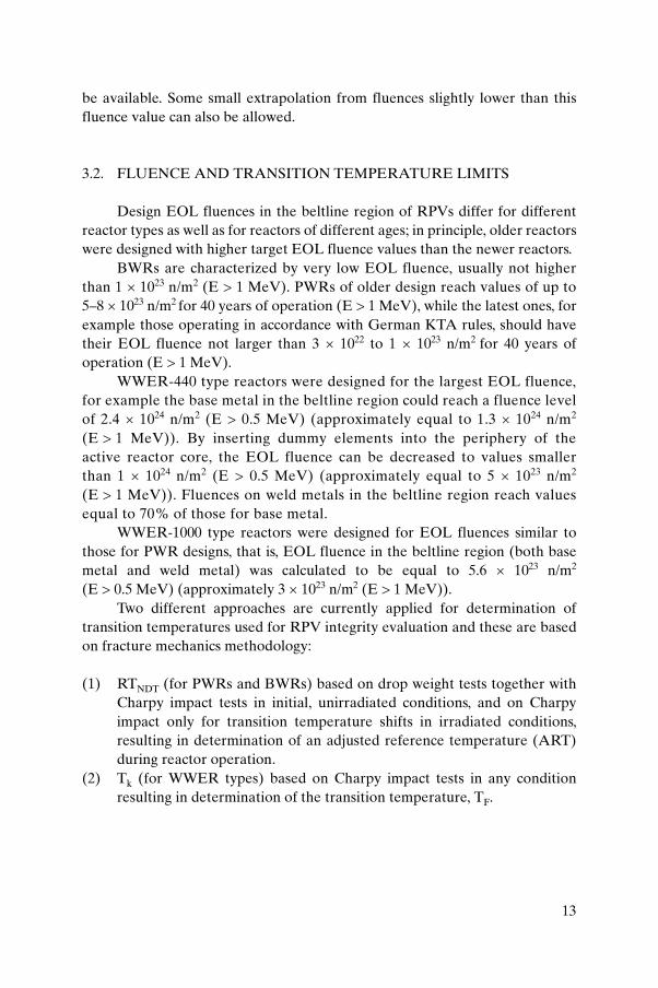
3.2. FLUENCE AND TRANSITION TEMPERATURE LIMITS
Design EOL fluences in the beltline region of RPVs differ for different reactor types as well as for reactors of different ages; in principle, older reactors were designed with higher target EOL fluence values than the newer reactors.
BWRs are characterized by very low EOL fluence, usually not higher than 1 × 10²³ n/m2 (E > 1 MeV). PWRs of older design reach values of up to5–8 × 10²³ n/m2 for 40 years of operation (E > 1 MeV), while the latest ones, for example those operating in accordance with German KTA rules, should have their EOL fluence not larger than 3 × 10²² to 1 × 10²³ n/m2 for 40 years of operation (E > 1 MeV).
WWER-440 type reactors were designed for the largest EOL fluence, for example the base metal in the beltline region could reach a fluence level of 2.4 × 1024 n/m2 (E > 0.5 MeV) (approximately equal to 1.3 × 1024 n/m2
(E > 1 MeV)). By inserting dummy elements into the periphery of the active reactor core, the EOL fluence can be decreased to values smaller than 1 × 1024 n/m2 (E > 0.5 MeV) (approximately equal to 5 × 10²³ n/m2
(E > 1 MeV)). Fluences on weld metals in the beltline region reach values equal to 70% of those for base metal.
WWER-1000 type reactors were designed for EOL fluences similar to those for PWR designs, that is, EOL fluence in the beltline region (both base metal and weld metal) was calculated to be equal to 5.6 × 10²³ n/m2
(E > 0.5 MeV) (approximately 3 × 10²³ n/m2 (E > 1 MeV)).Two different approaches are currently applied for determination of
transition temperatures used for RPV integrity evaluation and these are based on fracture mechanics methodology:
(1) RTNDT (for PWRs and BWRs) based on drop weight tests together with Charpy impact tests in initial, unirradiated conditions, and on Charpy impact only for transition temperature shifts in irradiated conditions, resulting in determination of an adjusted reference temperature (ART) during reactor operation.
(2) Tk (for WWER types) based on Charpy impact tests in any condition resulting in determination of the transition temperature, TF.
13

In both cases, irradiated transition temperatures (ART and TF) can be developed using code/regulatory formulas or surveillance specimen data if they fulfil given code requirements and conditions.
Transition temperature limits are not usually explicitly defined in RPV codes and standards. A high transition temperature may affect operating P–T limits for normal operation as well as hydrotests and compliance with established pressurized thermal shock (PTS) limits.
PTS integrity evaluations will be required if the maximum allowable transition temperatures of beltline materials at design EOL fluence are exceeded in the following cases:
(a) Deterministic approach:(i) In France and Germany the maximum ART is around 100°C,
depending on applied safety factors and in-service inspection programme results. The latest version of KTA 32 (applied only to the newest KONVOY type reactors) contains a requirement that the maximum transition temperature shift due to operational conditions (mainly by irradiation) should not be larger than +30°C.
(ii) For WWER-440 (V-230 type): Tk
a(maximum TF for PTS) = 130–180°C.(iii) For WWER-440 (V-213 type) and WWER-1000:
Tka = 90–120°C for non-qualified, non-destructive examination
(NDE); and Tk
a = 120–150°C for qualified NDE.(b) Probabilistic approach:
Used for US plants in accordance with Ref. [14]. Two cases are distinguished for the relation between material transition temperature, ART and limit temperature, defined as ‘screening criteria’:
(i) If ART < Tscreening = 121°C for axial welds or 149°C for circumferential welds, then no further evaluation is required.
(ii) If this requirement is not fulfilled, then a full computation of RPV failure probability must be performed (according to NRC Regulatory Guide 1.154). It should be noted that an extensive re-evaluation of the PTS screening criteria is now under way in the form of a joint programme between the NRC and the Electric Power Research Institute (through the EPRI’s Materials Reliability Program).
14

3.3. APPLICATION ISSUES
3.3.1. P–T curves
Current codes require that allowable P–T curves for RPVs operating under normal and hydrotest (pressure and leakage) conditions are calculated using a postulated defect that is usually set to be equivalent to a semi-elliptical surface crack extending to a depth equal to one quarter of the vessel thickness, using the ASME Section XI KIC (static crack initiation) curve and a safety factor of two on pressure loads. The stress intensity factors, KI, are determined for the following representative materials:
(a) PWR – A 533B-1: Sm ~ 200 MPa, t = 250 mm, a = 62.5 mm, KI = 100 MPa·m0.5.
(b) WWER-440 –15Kh2MFA: s = 200 MPa, t = 140 mm, a = 35 mm, KI = 75 MPa·m0.5.
(c) WWER-1000 –15Kh2NMFA: s = 220 MPa, t = 190 mm, a = 47.5 mm, KI = 95 MPa·m0.5.
Using these KI values the utilities can define the hydrotest temperature and the P–T curve for each vessel accordingly, with consideration given to the level of ageing due to irradiation embrittlement.
3.3.2. PTS
The integrity of the RPV during PTS is calculated in accordance with two primary approaches:
(1) Deterministic: All potential regimes are evaluated, during which stresses can reach values up to the yield strength of the RPV material while temperatures, at the final stage of PTS, can be as low as those of water coolant from the emergency core cooling system or additional injection tanks. Postulated defects differ in their size, density and form depending on the plant design and code used, as well as on conditions of in-service inspection procedures and quality (existence of qualification procedure, etc.). Examples of such postulated defects are as follows:(a) PWR (France): Elliptical defect of underclad type with height (2a)
equal to 6 mm, corresponding to the value of performance demonstration of NDE.
(b) PWR (Germany): Semi-elliptical defect of through clad type with height equal to 25 mm and some other sizes for sensitivity studies.
15

(c) WWER-440 and 1000:(i) Without NDE qualification: semi-elliptical surface defects with
depths of up to 0.25t, i.e. a = 35 mm for WWER-440 and a = 47.5 mm for WWER-1000.
(ii) With NDE qualification: underclad elliptical defect with a height of up to 0.1t, i.e. 2a = 14 mm for WWER-440 and 2a = 20 mm for WWER-1000.
(2) Probabilistic: Two cases can be distinguished depending on the relation between the material transition temperature, ART, and the limit temperature, defined as screening criteria. For US plants in accordance with US regulations:(a) If ART < Tscreening = 121°C for axial welds (149°C for circumferential
welds), then no further evaluation is required [14].(b) If this relation is not fulfilled, then a probabilistic evaluation of RPV
failure probability should be performed (Regulatory Guide 1.154). In this case, various defect types and sizes (semi-elliptical surface breaking, underclad elliptical, etc.) are taken into account with a specified density and location through the RPV thickness. The estimated failure probability of the RPV is then compared with an established risk goal.
3.3.3. Transferability of toughness values
In the assessment of RPV integrity, the effect of constraint on fracture toughness and subsequently on the reference temperature (T0) value should also be taken into account. Considerations include:
(a) Postulated defects of reduced size (0.1 of wall thickness or less) are characterized by quite different constraint values than defects with ‘standard’ assumed defect depths (0.25 of wall thickness) or even cracks in standard test specimens (nominally 0.5 of specimen width).
(b) Smaller defects result in higher fracture toughness values and thus a lower T0.(c) Biaxial loading of small defects results in higher constraint that decreases
fracture toughness values and increases the T0 value.(d) Different fracture toughness specimen loading (resulting from their
sample form) produces a bias. For example, the difference between reference temperatures determined from compact tension specimens and those from three-point bending specimens is usually considered to be within 5–15°C. Results from three-point bending specimens may be non-conservative (i.e. lower T0) compared with compact tension specimens, but conservative relative to the RPV.
16

3.3.4. Acceptability of defects found during in-service inspection
Indications of defects found during in-service inspections of RPVs that are larger than those allowed by appropriate codes (ASME Section XI, French RSEM, or others for WWER RPVs) must be evaluated to determine their impact on RPV integrity. Defects may be distributed throughout the whole thickness of the RPV and located in the base metal as well as the weld. Their sizes are, as a rule, smaller and their number significantly less than those used as postulated defects. However, conservative flaw distributions are generally utilized to provide for generic application to more RPVs.
3.4. MASTER CURVE APPROACHES
For the different applications described above, P–T curves, PTS screening criteria, deterministic or probabilistic approaches, in-service flaw evaluation and ageing management of plants, an essential requirement is the determination of RPV toughness for the materials at different locations in a given RPV.
For all cases, the following questions are relevant:
(a) What is the material initial toughness value?(b) What are the temperature and fluence levels at the different locations in
the vessel?(c) What are the consequences of irradiation embrittlement on the reference
temperature and the toughness versus temperature curve?(d) What are the uncertainties and how can data from the same vessel or
other, similar, vessels be used? (e) How can the surveillance programme data be used? (f) How can small specimen results be extrapolated to the full size structure?
For all of these questions the Master Curve approach can provide valuable information.
17

4. DETERMINATION OF T0
Guidelines for the determination of T0 are based on ASTM E 1921-02 entitled Test Method for Determination of Reference Temperature, T0, for Ferritic Steels in the Transition Range [5], and include specific recommendations regarding:
(a) Test apparatus;(b) Specimen configuration, dimensions and preparation;(c) Test procedure;(d) Calculation of fracture toughness values;(e) Prediction of specimen size effects and transition temperature;(f) Precision and bias;(g) Methods, test equipment, loading devices, measurement of load and
displacement.
ASTM E 1921-02 also considers special fracture events such as ‘pop-ins’ and outliers. This section covers the general structure for the determination of cleavage fracture toughness values, KJc, and the evaluation of T0 for practical use. Figure 2 is a flow chart for determination of T0 and also for identification of the main technical issues.
4.1. GENERAL EVALUATION PROCEDURE FOR T0 DETERMINATION
In this section the general evaluation procedure of the test results is summarized.
4.1.1. Fracture toughness evaluation
The J-integral at the onset of cleavage fracture, Jc, of the test datum is determined according to Eq. (2) and following the recommendations in paragraph 9.1 of ASTM E 1921-02:
(2)
where Je is the elastic component of the J-integral and Jp is the plastic component of the J-integral.
J = J + Jc e p
18

The Jc values are transformed into plain strain cleavage fracture toughness values, KJc, using Eq. (3):
(3)
where E is Young’s modulus and n is Poisson’s ratio for steel (0.3).
4.1.2. Validity check
The test specimens and the initial crack size (a0) and straightness shall fulfil the requirements defined in ASTM E 1921-02. The measured KJc values shall be checked to determine if they fulfil the defined validity criteria. A KJc
datum is invalid if the specimen size requirement of Eq. (4) is exceeded:
(4)
where
b0 is the initial specimen ligament (W–a0);M is the constraint value in ASTM E 1921-02 (set equal to 30);sys is the material yield strength at the test temperature.
In addition to the size requirement there is the maximum ductile crack growth criterion of 0.05(W–a0) or 1 mm, whichever is the smaller, where a0 is the initial crack length and W is the specimen width. Those KJc values above the validity criteria shall be censored to the validity limit. Should both the KJc(limit) and the maximum ductile crack growth validity criteria be violated, the lower value of the two shall prevail for censoring purposes.
4.1.3. Prediction of size effects and transition temperature
The basis of the Master Curve approach is a three parameter Weibull model which defines the relationship between KJc and the cumulative probability of failure, pf (Eq. (5)):
(5)
K = J E
1J c c 2- n
K = Eb
MJc(limit)0 yss
n( )1 2-
p = 1 expK K
K Kf1 min
0 min
– ---
Ê
ËÁˆ
¯̃
È
ÎÍÍ
˘
˚˙˙
4
19

where
pf is the cumulative probability of failure;KI is the fracture toughness of the material;Kmin is the theoretical lower bound fracture toughness set at 20 MPa·m0.5 in
ASTM E 1921-02;K0 is the scale parameter.
The statistical weakest link theory is used to model the effect of specimen size on the probability of failure in the transition range. In the next step, the measured KJc values are adjusted to a specimen size, 1T (25.4 mm), using Eq. (6):
(6)
where
B0 is the thickness of the tested specimen (side grooves are not considered);B1T is the thickness B = 1T (25.4 mm);KJc(1T) is the fracture toughness of a specimen with a thickness of B = 1T;KJc(X) is the fracture toughness of the tested specimen;Kmin is the lower bound fracture toughness fixed at 20 MPa·m0.5 in ASTM
E 1921-02.
The lower validity criterion for the Weibull statistics, on which the Master Curve is based, is 50 MPa·m0.5. The KJc values below 50 MPa·m0.5 need not be size adjusted (see Section 4.3.3).
4.1.4. Determination of T0
The value of T0 is calculated after inclusion of all valid and censored values according to the single or multitemperature methods:
Single temperature evaluation. Evaluation of the scale parameter, K0, is performed according to Eq. (7) and the fracture toughness for a median (50%) cumulative probability of fracture, KJc(med), according to Eq. (8) of a data set at the applied test temperature:
K = K K KB
BJc(1T) min Jc(X) min0
1T
1/4
+ ÈÎ ˘̊ Ê
ËÁˆ
¯̃–
20

1/4
(7)
where KJc(i) is the individual KJc(1T) value and N is the number of KJc values.The term N is replaced by the number of valid KJc values, r, if censored
KJc values are included in the calculation:
(8)
The KJc(med) value determined for the data set at test temperature is used to calculate T0 at KJc(med) of 100 MPa·m0.5 by Eq. (9):
(9)
Multitemperature evaluation. The multitemperature option of ASTM E 1921-02 represents a tool for the determination of T0 with KJc values distributed over a restricted temperature range, namely, T0 ± 50oC. The value T0 can be evaluated by an iterative solution of Eq. (10):
(10)
where
Ti is the test temperature corresponding to KJc(i);di is the censoring parameter: di = 1 if the KJc(i) datum is valid (Eq. (4)) or
di = 0 if the KJc(i) datum is not valid and censored.
4.1.5. Establishment of the transition temperature curve (Master Curve) and tolerance bounds
Values of KJc tend to conform to a common toughness versus temperature curve shape expressed by Eq. (11):
K = K K
NK0
Jc(i) min
4
i=1
N
min
–( )È
Î
ÍÍÍ
˘
˚
˙˙˙
+Â
K = K (K K )(ln 2)Jc(med) min 0 min1/4+ –
T = T1
0.019ln
K 30
700Jc(med)–
–ÊËÁ
ˆ¯̃
Ê
ËÁˆ
¯̃
d i i 0
ii
n
Jci
T T
T T
K K
exp .
exp .
m
0 019
11 77 0 019 01
-( )ÈÎ ˘̊
+ -( )ÈÎ ˘̊
--
=Â
iin exp .
exp .
( ) -( )ÈÎ ˘̊
+ -( )ÈÎ ˘̊{ }=
=Â
4
51
0 019
11 77 0 019
T T
T T
i 0
i 0i
n
00
21

22
(11)
Both upper and lower tolerance bounds can be calculated using Eq. (12):
(12)
where 0.xx represents the cumulative probability level.
4.2. SEQUENCE OF T0 DETERMINATION
4.2.1. Selection of test temperatures and testing of specimens
ASTM E 1921-02 defines a validity ‘window’ for the Master Curve (Fig. 3) in terms of the maximum KJc capacity, KJc(limit), of the tested specimen and a temperature range of T0 ± 50oC. Before testing, an estimation of this validity window is necessary for the specific material and specimen size. As presented in Section 4.1.2, the KJc(limit) value is calculated using Eq. (4). In a second step, the expected T0 is to be estimated. This estimated T0 is also used to define the range of test temperatures for the first tests. ASTM E 1921-02 recommends that the selected test temperature should be close to T0 or where the KJc(med) value for a 1T-sized specimen is about 100 MPa·m0.5. Following ASTM E 1921-02, Charpy V-notch data can be used as an aid for predicting a viable reference temperature, T0(est)#1, according to Eq. (13):
(13)
where
TCVN is the Charpy V-notch transition temperature corresponding to a 28J or 41J Charpy V-notch impact energy;
C is the constant tabulated in ASTM E 1921-02 for different specimen sizes.
For precracked Charpy-sized specimens mainly used in RPV surveillance programmes, C is recommended to be –50oC (T28J) or –56oC (T41J), respectively. For testing of irradiated material the prediction formulas of the specific codes can be used to estimate the transition temperature shift caused by neutron irradiation. The neutron irradiation induced Charpy transition temperature shift generally corresponds to the T0 shift to a sufficient degree of accuracy.
K T TJc(mean)1T 0= + -( )ÈÎ ˘̊30 70 0 019exp .
K 20 ln1
1 0.xx11 77exp 0.019(T T )Jc(0.xx)
1/4
0= + ÊËÁ
ˆ¯̃
ÈÎÍ
˘˚˙ + -ÈΖ
˘̊̆{ }
T T C0(est)#1 CVN= +

owing to metallurgical heterogeneities. Thus, KJc values may be scattered, in particular when small Charpy-sized specimens are tested. The test temperature chosen on the basis of Charpy V-notch or fracture toughness data should be verified with at least two tests. In the examination of specimens with a thickness smaller than 1T (25.4 mm), the fact that T0 applies to 1T-sized specimens needs to be taken into account. As small specimens give higher KJc values than larger specimens at a selected test temperature, they have to be tested at lower temperatures (see Eq. (6)).
Using this first KJc data point, a preliminary reference temperature, T0(est)#2, can be calculated according to the single or multitemperature method, depending on the selected test temperatures. The estimated temperature range for the remaining tests becomes T0(est)#2 ± 50oC. This temperature range is dependent on specimen size. Small specimens have a low validity limit according to Eq. (4). For these specimens, the selected test temperature of the remaining specimens should be at or below T0(est)#2. The whole temperature range, T0(est)#2 ± 50oC, can only be used with sufficiently large specimens. If the single temperature method is used, all specimens have to be tested at the same temperature. This means that in some cases the pretests cannot be used for the evaluation. The advantage of the multitemperature method is that test
0
50
100
150
200
250
-75 -50 -25 0 25 50 75
Frac
ture
tou
ghne
ss K
Jc (M
Pa·
m0.
5 )
T-T0 (K)
KJc(0.95)
KJc(med)
KJc(0.05)M=30
FIG. 3. Example of the validity window of a precracked Charpy-sized specimen of RPV steel.
23

temperatures can be selected from within the estimated temperature range. The application of the multitemperature method is also more effective and saves test specimens, since all tested specimens can be considered in the T0
calculation. The minimum number of valid KJc data points required for the T0
evaluation is six.
4.2.2. Determination of T0 (ASTM E 1921)
As indicated in Sections 4.1.4 and 4.2.1, the procedure for the determination of T0 according to ASTM E 1921 includes both single and multitemperature approaches. When the single temperature method is used, a number of specimens are tested at the same temperature and the KJc data are evaluated using Eqs (7–9). In the multitemperature method, the KJc data determined at different test temperatures are evaluated according to Eq. (10).
4.2.3. Checking the validity of T0 (ASTM E 1921-02)
ASTM E 1921-02 stipulates validity criteria for T0 determination. The following weighting system from ASTM E 1921-02 specifies the required minimum number of valid KJc data points:
(14)
where
ni is the specimen weight factor as a function of T – T0 according to Table 1;ri is the number of valid KJc tests within T – T0 range i (Table 1).
If the determined T0 is not valid, additional specimens have to be tested until the weight factor requirement is fulfilled. For the single temperature method, additional specimens have to be tested at the chosen test temperature. However, it is more effective to change to the multitemperature method. This allows adjustment of the test temperature for the additional tests in the range with the highest weight factor mentioned in Table 1. For the multitemperature method, the test temperatures as well as those of the first specimens should preferably lie in the range with the highest weight factor mentioned in Table 1.
r ni ii
3
=Â ≥
1
1
24

4.3. ANALYSIS OF ABNORMAL FRACTURE TOUGHNESS DATA
The Master Curve method has in general been shown to be applicable in its basic form to a variety of ferritic base and weld metals with microstructures and properties which may result from very different manufacturing and operational histories, including special heat treatments and exposure to thermal ageing and/or neutron irradiation [15]. The transition range fracture toughness is also relatively insensitive over a wide range of mechanical properties and microstructure characteristics. This means that a similar fracture toughness versus temperature dependence, as is assumed in the basic Master Curve model, can be used in most cases. Even measures that decrease the toughness of the steel, such as special heat treatment or neutron irradiation, do not generally degrade the consistency of the measured fracture toughness versus temperature behaviour with that predicted by the model.
Although the model has been applied mainly to quenched and tempered low alloy structural steels, normally those possessing high strength and at least moderate toughness, more specific and/or more alloyed steel types such as ferritic stainless steels or steels with low ductility have followed, at least moderately, the Master Curve estimation [16].
Even ferritic steels with very high ductile to brittle transition temperatures following, for example, a tempering treatment or a high neutron fluence, have usually shown quite ‘normal’ fracture behaviour in regard to both scatter and temperature dependence, confirming the general validity of the basic Master Curve model. In general, the model has been applied successfully to the most common Western and several WWER-440 and WWER-1000 type RPV base and weld metals, as well as to surveillance data measured with miniature fracture mechanics specimens [17].
Despite its good general applicability, special cases have been recognized where the Master Curve method should be adjusted or modified, or where the method should not be applied at all. The following cases have been identified:
TABLE 1. WEIGHT FACTORS FOR T0 ANALYSIS
(T – T0) range (°C)
1T KJc(med) range(MPa·m0.5)
Weight factor(ni)
50 to –14 212–84 1/6
–15 to –35 83–66 1/7
–36 to –50 65–58 1/8
25

(a) Inhomogeneous materials or materials with a dual or multiphase microstructure which consists of large areas of phases having very different properties. These cases can usually be estimated with the Master Curve by adopting a modified scatter band model for fracture probability.
(b) Materials which are susceptible to grain boundary fracture may exhibit fracture behaviour which does not follow the Master Curve prediction if the proportion of grain boundary fracture is high.
(c) The fracture behaviour outside the standard temperature region (–50oC £T – T0 £ 50°C) will often, but not always, follow the Master Curve model. In certain cases these extrapolations may be used, although this option is not included in the ASTM E 1921-02 standard. Deviations from the predicted behaviour are often associated with special situations which should be recognized before the extrapolation.
4.3.1. Inhomogeneous materials
4.3.1.1. General
The Master Curve approach is based on the weakest link theory [4], in which the material is assumed to contain randomly distributed defects or cleavage fracture initiators. It is assumed that the material is macroscopically homogeneous, having uniform and isotropic strength and toughness properties. In addition to macroscopic homogeneity, the material is assumed to have an essentially single phase microstructure. Significant deviations from either or both of these assumptions may result in anomalous fracture behaviour, in comparison with ‘homogeneous’ materials, which does not comply with the predicted behaviour.
Macroscopic inhomogeneity typically appears as an excessive scatter exceeding that shown by the Master Curve model. On the other hand, both the temperature dependence of KJc and the T0 estimation are typically not very sensitive to macroscopic inhomogeneity, or may even be totally unaffected. The same kind of behaviour is expected of materials with a (virtually) two phase structure, caused, for example, by large non-metallic inclusions or other impurities, which may result in an excessive scatter in KJc data if the specimen size is small in relation to the size of these particles.
Macroscopic inhomogeneity may exist, for example, in cross-sections of multipass welds between the beads of the weld or between the weld metal and the heat affected zone material. Similarly, large components such as forgings and thick, hot rolled plates may experience macroscopic inhomogeneity in the thickness direction. If macroscopic inhomogeneity is known to exist at different locations and/or orientations in a component or structure, the Master Curve
26

analysis should, if possible, be performed separately for each relevant area and orientation with approximately uniform properties. Depending on the application and the consistency of the experimental versus predicted behaviour, an adjusted Master Curve analysis can be performed to ensure the quality of the estimation.
Whenever necessary, the consistency of any measured data with the Master Curve standard prediction, namely, whether the material should be analysed as an inhomogeneous case, can be checked by applying the structural integrity assessment procedure (SINTAP) [18]. If abnormal behaviour is encountered, the data should be analysed with the modified Master Curve model and included in the SINTAP procedure, which takes into account the material inhomogeneity. The procedure is described step by step in Appendix II.
4.3.1.2. Procedure for inhomogeneous materials (SINTAP)
The Master Curve extension, hereafter referred to as the SINTAP procedure, has been developed and introduced for statistically analysing the fracture behaviour of inhomogeneous steels. The procedure can be applied, for example, to welds where the heat affected zone has areas of localized brittleness. The method is briefly described below.
The procedure consists of three steps, each setting a different validity level for that part of the data that is to be censored. The whole data set is used in the analysis, only a certain a priori assumption is made concerning the nature of the data being censored. The procedure guides the user towards the most appropriate fracture toughness estimate, KMAT, of the material. In the last stage, the final KMAT fracture toughness estimate and its probability distribution are calculated according to steps 1, 2 or 3 below.
Step 1: Normal maximum likelihood (MML) estimation. All data are used for the estimation, with the exception of results from ductility tests ending in non-failure, which are affected by large scale yielding. Data censoring shall be performed according to ASTM E 1921-02.Step 2: Lower tail MML estimation. The 50% upper tail of the data set is censored and the remaining data (corresponding to a cumulative probability of 50% or less) are used for MML estimation of KMAT or T0(KMAT). This ensures that the estimate is descriptive of the material (i.e. microscopic properties), without being affected by macroscopic inhomogeneity, ductile tearing or large scale yielding (i.e. unrealistically high ‘apparent’ toughness values). Step 2 proceeds as a continuous iterative process until a ‘constant’ level has been reached for K0 or T0.
27
Step 3: Minimum value estimation. Only the minimum toughness value (i.e. one value corresponding to one single temperature) in the data set is used for the estimation. The intention is to assess the significance of a single minimum test result, with the aim of avoiding non-conservative fracture toughness estimates which may arise if median (50%) fracture toughness is used for a material exhibiting significant microscopic inhomogeneity.
Step 3 sets criteria to the allowable differences between the median (50%) and the lower bound (5%) fracture toughness levels. Provided that the resultant KMAT or T0(KMAT) estimate according to step 3 is more than 10% lower or 8°C higher, respectively, than the corresponding estimate according to step 1 or 2, whichever of them is lower (KMAT) or higher (T0(KMAT)), this single minimum value is regarded as significant and the estimate according to step 3 is taken as a final estimate of the material’s fracture toughness. Otherwise, the lowest (highest) one of the estimates given by steps 1 and 2 is taken as a final estimate.
4.3.1.3. Evaluation of data for possible inhomogeneity
The need to adopt the SINTAP procedure depends mainly on the application for which the data are to be used. As the effect of inhomogeneity appears mainly or merely in the scatter of fracture mechanics data, rather than in the value of T0 or the temperature dependence of KJc, it is recommended that the SINTAP procedure be performed in all cases where the lower bound fracture toughness, determined as a function of T0, or any value based on the true data scatter, is to be used. Such applications are typically associated with the integrity assessment of components and structures.
In cases where the absolute value or the shift of T0 is to be used instead of a tolerance bound, the Master Curve analysis can usually be performed without applying the SINTAP procedure. Such applications are, for example, those where the degradation of material properties (in nuclear applications typically after exposure to thermal ageing or neutron irradiation) are investigated by comparing the shift values of T0 measured for different material conditions.
It is, however, recommended that the SINTAP procedure be adopted in all cases where data (one or more valid KJc values) fall outside the 2% tolerance bound. The existence of such outliers may be an indication of inhomogeneity.
The general procedure for analysing fracture toughness data is depicted in Fig. 4. Examples detailing the application of the procedure are given in Appendix II.
28

4.3.2. Grain boundary fracture
The Master Curve approach is based on a cleavage fracture model where the features characteristic of cleavage fracture initiation and propagation have been assumed. The existence of fracture modes other than cleavage usually means that the factors controlling the propagation of fracture differ more or less from those typical of the cleavage mode. Experience, however, has shown that the quality of the Master Curve estimation is not very sensitive to mixed or quasi-cleavage fracture modes, especially if the proportion of other fracture modes is not very large. Attention should be paid to the possible existence of grain boundary fracture, which cannot necessarily be deduced directly from measured fracture toughness data without fractographic investigation. Extensive grain boundary fracture (due to segregation of impurity elements) may exist, for example, as a result of improper tempering of certain types of quenched steel, exposure to high neutron fluences, or thermal ageing.
Grain boundary fracture may be a stress or strain controlled event, depending on temperature, which means that the deviation from typical
(1) Determination of T0 and the data scatter curves using the basic Master Curve procedure (2) Determination of the 2% tolerance bound if needed (3) Separate analysis areas with uniform microstructure and properties if needed
Application using a lower bound curve
Application using absolute T0 or its shift
Check of outliers applying the 2% tolerance bound criterion
No outliers Outliers exist
Application of the normal T0 Master Curve estimation
Outliers exist
T0 and data scatter refinement using the SINTAP procedure
Application of the SINTAP adjusted T0 and scatter bound estimation
FIG. 4. The general procedure for analysing materials which may indicate fracture behaviour affected by macroscopic inhomogeneity or exceptional phase structures.
29

cleavage fracture behaviour tends to depend on temperature. Even materials with 100% grain boundary fracture have been shown to follow the Master Curve if the T0 value is low, namely, less than about 0oC, when the fracture is likely to be stress controlled rather than strain controlled. At higher temperatures where grain boundary fracture becomes strain controlled and is thus not expected to be significantly affected by temperature, the application of the Master Curve is not recommended. However, moderate amounts (less than 50%) of grain boundary fracture have not been observed to affect the Master Curve analysis.
Only data from a few experimental investigations on the characteristics of grain boundary fracture toughness, covering the whole transition region from the lower to upper shelf, are available. It is recommended that additional testing be performed in cases where grain boundary fracture is likely or suspected of being possible. In such cases, more tests than those prescribed in ASTM E 1921 should be performed at relevant temperatures. Examples of the analysis of the fracture toughness data of materials prone to grain boundary fracture are given in Appendix II.
4.3.3. Extrapolation outside the standard validity window
The extrapolation of fracture toughness estimation outside the standard temperature region (–50°C £ T – T0 £ +50°C) is possible if exceptional fracture behaviour outside this region is anticipated.
The primary concern with application outside of the standard temperature range (–50°C £ T – T0 £ +50°C) is connected to the fact that so far there has been no theoretical model to explain the invariance of the Master Curve temperature dependence. Although the majority of ferritic steels behave in accordance with the Master Curve, there have been a few cases where the temperature dependence has appeared to be less or more than that predicted by the Master Curve model. Typically, these steels have had a very high T0
(> +150ºC) or a very low T0. In such cases, the deviation from the Master Curve prediction has usually, but not always, been observed to result from ductile crack propagation.
Until a theoretical explanation has been finalized, care should be taken in applying the Master Curve outside this ‘validity’ region. Since the size effect and scatter are unaffected by the temperature dependence, the Master Curve method can be applied in assessments outside the –50°C £ T – T0 £ +50°C temperature region, but temperature extrapolations should be avoided. General principles and background data for assessing the extrapolation and examples showing predictions outside the validity limits are given in Appendix II.
30

4.4. UNCERTAINTY IN T0 AND LOW BOUND CURVE FOR KJc
The uncertainty in determining T0 depends on the number of specimens used to establish the value. The uncertainty is defined according to a standard two-tail normal distribution with two basic variables, i.e. the test temperature and the number of specimens used for the T0 determination, as follows:
(15)
where
b = 18–20oC, depending on the value of T – T0 (single temperature data — when KJc(med) is equal to or greater than 83 MPa·m0.5, b = 18oC);
r is the number of valid (uncensored) test results used to determine T0;Z is the confidence level (Z85% = 1.44).
Alternatively, a b value of 20oC can be used for all values of KJc(med) but not for values less than the minimum (58 MPa·m0.5). The exact value of b can be determined from KJc(med) according to ASTM E 1921-02.
The lower and upper tolerance bounds (KJc(0.xx)) for the estimated fracture toughness in KJc = f(T) are calculated from a revised T0(T0(margin)) as follows:
(16)
(17)
where 0.xx is the selected cumulative failure probability (in %/100). For 1%, 2% and 5% cumulative failure probabilities the bounds are as
follows:
(18)
(19)
DTr
Z0 =b
T T T0(margin) 0 0= + D
Kxx
T TJc(0.xx) mar= +-
ÊËÁ
ˆ¯̃
ÈÎÍ
˘˚˙ + -20
11 0
11 77 0 0191 4
0ln.
exp ./
( ggin)( )ÈÎ
˘˚{ }
K 23.5 24.4exp 0.019 T TJc(0.01) 0(margin)= + -( )ÈÎ
˘˚
K 24.1 29.0exp 0.019 T TJc(0.02) 0(margin)= + -( )ÈÎ
˘˚
31

(20)
When the data set consists of several test temperatures, the formula proposed by SCK·CEN [19] for determining the median fracture toughness (KJc(med)) can be used:
(21)
where r is the number of valid test data. The median KJc is used to determine the b parameter and the uncertainty
of T0 according to ASTM E 1921-02. When KJc(med) is equal to or greater than 83 MPa·m0.5, b corresponds to 18oC. Alternatively, a b value of 20oC can be used for all values of KJc(med) not less than the minimum (58 MPa·m0.5).
5. DETERMINATION OF T0 FOR RPV MATERIAL
5.1. METHODOLOGY TO DETERMINE T0 FOR RPV MATERIAL
Fracture toughness tests to determine properties for engineering analysis are necessarily destructive and must be performed on a representative sample of the structural material. Ideally, the samples for destructive testing are removed from the sections of material used to fabricate the structure. This type of sampling is standard practice in many engineering applications. In an RPV, this sampling often involves taking plate or forged materials from sources of excess materials such as nozzle cut outs. Weld samples are often taken from test welds fabricated from the same source materials (weld wire and flux) using the vessel fabrication procedures. However, fabrication of a vessel from plate material requires welding of multiple plates and often involves more than one source of welding material. In these cases, samples of material are removed from the materials with the highest projected irradiation sensitivity. Although fewer base materials and welds are involved in the fabrication of a vessel from forgings, properties may vary significantly from region to region within a single forging. In all cases, care must be taken to ensure that the sampled material is representative of the structure.
K 25.2 36.6exp 0.019 T TJc(0.05) 0(margin)= + ( )ÈÎ
˘˚–
Kr
T TJc(med)eq
ii
r
= + -( )ÈÎ ˘̊{ }=Â1
30 70 0 019 01
exp .
32

The baseline properties of an RPV are determined by testing materials identified during the vessel qualification programme. Charpy V-notch and other small specimen tests are used to estimate the linear elastic fracture toughness (KIC) transition curve. Local procedures for characterizing the fracture toughness transition curve are defined according to national codes and regulations.
One common practice used in preservice integrity analysis of an RPV is outlined in ASME Section III [20]. This procedure uses measured values of the reference temperature, RTNDT (as defined using Charpy V-notch and drop weight test results), to determine lower bound estimates of the fracture toughness from the ASME KIC reference curve. The reference curve is based on an empirical analysis of the relationship between measured RTNDT values and measured KIC values. The curve is considered to be sufficiently conservative such that measured RTNDT values are used directly in RPV integrity analysis without further adjustments for material variability. Master Curve testing can also be performed on unirradiated sample material to determine T0. ASME Code Cases N-629 [7] and N-631 [21] have recognized the Master Curve based reference temperature RTT0 as an alternative means of indexing the KIC reference toughness curve. This sampling procedure should be sufficient for preservice integrity analysis in the context of ASME Section III.
Evaluation of pressure vessel integrity in WWER plants is based on a similar set of curves that are matched to experience with the steels used in this fleet of reactors but indexed to the critical temperature of brittleness, Tk, on the basis of Charpy impact tests alone. Similar procedures for estimating the fracture toughness transition are used in Japan. Both the WWER and Japanese approaches have multiple curves for describing different types of material. However, all of the reference toughness curves have similar shapes and describe the same basic behaviour. These shapes are consistent with the Master Curve shape.
Determination of irradiated properties for in-service integrity analysis is generally based on the testing of surveillance specimens. The sampled materials used for the surveillance programme are generally taken from the same source as the materials used to determine the unirradiated properties. However, the relationship between the irradiated sample material and the vessel is complicated by three factors:
(1) The state of mechanical constraint in the specimens used to measure fracture toughness may not match the mechanical constraint on a flaw in the vessel.
(2) The irradiation conditions of the surveillance material may not match the conditions of interest in the vessel. While differences in neutron fluence
33

are commonly recognized, other factors such as neutron flux or irradiation temperature may also contribute to discrepancies between the vessel and sample material.
(3) The radiation sensitivity of the pressure vessel steels is controlled by small variations in impurity elements (e.g. Cu and P), which can vary significantly within a single heat of material.
While measurements on unirradiated sample materials can be directly applied to the vessel, measurements on the same materials in the irradiated condition must be adjusted to take account of these three factors. These adjustments are required for both Charpy based estimates of fracture toughness and Master Curve based estimates.
The development of Master Curve test procedures has made it feasible to determine fracture toughness transition temperatures in irradiated materials. The capability to observe directly the fracture toughness transition in materials that more closely approximate the in-service vessel condition is the primary advantage of the Master Curve approach. This advantage derives primarily from the capability to determine fracture toughness values from Charpy-sized specimens. Although the small Charpy-sized specimens meet the current testing requirements for T0 determinations, it has been widely observed that T0
values measured in Charpy-sized specimens are consistently 5–15oC lower than equivalent measurements made in larger compact tension specimens. This apparent bias has been attributed to the lack of constraint in the small Charpy specimens.
Adjustment of the measured T0 value to account for the Charpy bias may be required to apply the data to the vessel. Bias adjustments of T0 values measured in Charpy-sized specimens are required to match the data from larger compact tension specimens. It has been suggested that the bias may be related to the degree of triaxiality in the specimen and can be correlated with the T-stress. In this case, the apparent Charpy bias may be a function of specimen geometry rather than specimen size.
The reference toughness curves used for reactor integrity analysis are almost exclusively based on the testing of large compact tension specimens. Therefore, consistency with previous analyses may require a bias adjustment to the measured value. However, the stress state at the tip of a small flaw in a pressure vessel may not have the same ‘deep crack’ constraints as the compact tension specimen. Using the data to analyse relatively small flaws in pressure vessels may require consideration of the state of stress at the flaw tip. Further evaluation is required to determine the appropriate bias factor for RPV evaluations.
Prior to the development of Master Curve test procedures, the only significant source of information on irradiated transition temperatures was
34

Charpy testing of materials from reactor surveillance programmes. Numerous trend curves have been developed describing the irradiation induced shift in Charpy transition temperature as a function of the irradiation conditions and material composition. Procedures for adjusting measurements made on surveillance materials to reflect vessel conditions are generally based on these trend curves. In many applications, the trend curves are used in place of measured Charpy transition temperature shifts.
However, even with direct measurements, adjustments for differences in irradiation conditions and material composition are required. It would be preferable to base these adjustments on fracture toughness transition temperature trend curves. In fact, it would be preferable to adjust Charpy based measurements on the basis of fracture toughness trend curves. Unfortunately, the database of irradiated T0 determinations is not large enough to allow development of reliable fracture toughness transition temperature trend curves. The only basis for adjusting measured T0 values for differences in irradiation condition and material composition is the Charpy database.
Fortunately, experience with T0 testing has indicated a near 1:1 correlation between Charpy shifts and fracture toughness shifts. It is important to note that if this correlation did not exist the entire basis of the Charpy based approach to integrity analysis would be questionable. Given this correlation, it is possible to apply Charpy based adjustments to T0 measurements.
The Charpy adjustment may be applied to the measured T0 value in the following manner:
T0(FRPV, ΧRPV) – T0(FSM, ΧSM) ª DTCVN(FRPV, ΧRPV) – DTCVN(FSM, ΧSM)+ TCVN(0, ΧRPV) –TCVN(0, ΧSM) (22)
where
T0 is the Master Curve reference temperature; TCVN is the Charpy transition temperature;DTCVN is the Charpy transition temperature shift;FRPV, FSM are the irradiation conditions for RPV and sample material;CRPV, CSM are the material compositions of RPV and sample material.
In most cases, with representative sample materials, the difference in unirradiated Charpy transition temperature will be negligible. Equation (22) then reduces to:
T0(FRPV, ΧRPV) = T0(FSM, ΧSM) + [DTCVN(FRPV, ΧRPV) – DTCVN(FSM, ΧSM)] (23)
35

The Charpy transition temperature shifts can be determined from the appropriate trend curves. In this case, the measurement of T0 in the sample material becomes the baseline for the estimate in the irradiated pressure vessel. Ideally, the irradiation condition of the sample material should approximate the condition of the vessel. The accuracy of the approximation obviously increases as the size of the adjustment (the expression in brackets) decreases.
There is no single irradiation condition that characterizes the vessel beltline. In some cases, it may be possible to perform bounding calculations by using sample material measurements at fluences that exceed the expected peak vessel fluence, eliminating the need for an irradiation condition adjustment. In this case, Eq. (23) reduces to:
T0(FRPV, CRPV) £ T0(FSM, CSM) + [DTCVN(FSM, CRPV) – DTCVN(FSM, CSM)] (24)
This limiting calculation can be helpful when surveillance materials that correspond to the projected peak EOL fluence are available.
The measurement of T0 in an unirradiated sample material can be viewed as a special case of Eq. (23). If the unirradiated condition is used as the baseline for the adjustment, the corresponding Charpy shift for the sample material is obviously zero (DTCVN(0, CSM) = 0). In this case Eq. (23) reduces to:
T0(FRPV, CRPV) ª T0(0, CSM) + DTCVN(FRPV, CRPV) (25)
The estimated T0 for the vessel would be the sum of the unirradiated sample material measurement and the predicted Charpy shift for the vessel.
Multiple measurements of T0 in the sample material can be used to improve the reliability of the estimate. A baseline point for Eq. (23) can be established by fitting appropriate fluence dependence to the measurements. The baseline point may be taken at any point on the fitted curve, but in general should correspond to a fluence intermediate to the measured data.
5.2. EXAMPLE APPLICATION
The process of adjusting a measurement on a sample material to provide an appropriate estimate can be understood by considering the example case outlined in Table 2. In this case, a T0 value of 120oC was measured in a sample weld irradiated to a neutron fluence of 2.4 × 10²³ n/m2 (E > 1 MeV). The reactor vessel integrity analysis requires an estimated T0 value for the corresponding pressure vessel weld at 5.2 × 10²³ n/m2 (E > 1 MeV). The sample material was
36

irradiated in an accelerated fluence location, such that the high sample material fluence was accumulated in a relatively short time. The composition of the sample material was determined directly by making measurements on the tested material. The vessel composition was estimated by combining all relevant measurements on welds fabricated from the same heat of weld wire. As indicated in Table 2, there are slight differences between the measured sample material composition and the best estimate of the vessel weld composition.
A Charpy transition temperature prediction curve is required to apply the adjustments suggested in Eq. (23). The prediction curve is used to determine the predicted Charpy shifts for both the sample material condition and the reactor vessel condition. Table 3 compares predictions based on two widely used prediction curves (R.G. 1.99-2 and the Japanese model in JEAC 4021-2000 [10]). The NRC’s R.G. 1.99-2 contains a procedure for determining the Charpy shift based on a chemistry factor determined by the copper and nickel contents of the steel and a generalized fluence factor.
TABLE 2. IRRADIATION CONDITIONS AND MATERIAL PROPERTIES FOR SAMPLE WELD AND RPV WELD
Property Sample material Reactor vessel material
Weld heat WA100 WA100
Neutron fluence (E > 1 MeV) 2.4 × 10²³ n/m2 5.2 × 10²³ n/m2
Irradiation duration(effective full power years) 8 32
Irradiation temperature 290oC 285oC
T0 120oC (measured) To be determined
Composition Measured Best estimate
Copper 0.2 wt% 0.22 wt%
Nickel 0.6 wt% 0.65 wt%
Phosphorus 0.015 wt% 0.012 wt%
Silicon 0.25 wt% 0.3 wt%
37

6. FLUENCE PROJECTION INCLUDING ATTENUATION
6.1. INTRODUCTION
Having established a value for T0 at a neutron fluence for the material of interest, it will be necessary to determine T0 for the material at different fluences. This could involve both interpolation and extrapolation. Thus, a trend curve for prediction of embrittlement as a function of fluence is needed. This is not only required for projection to the inside surface of the RPV, but also for different locations within the RPV wall to allow for the establishment of P–T limits for reactor startup and integrity analyses during postulated accident conditions such as PTS. As most reactor cores do not have a circular configuration, the neutron flux varies at different points around the circumference of the RPV. Also, because the core does not occupy the entire height of the RPV, the flux also changes axially along the inner surface of the RPV.
Figure 5 illustrates examples of neutron fluence (E > 1 MeV) variation on the inner diameter of a typical PWR [13]. Figure 6 provides examples of neutron fluence (E > 0.5 MeV) variation of a typical WWER-440 RPV [23]. Owing to such variations, applications of neutron flux and fluence projections from surveillance locations to the RPV are more complicated. Moreover, because steel has a relatively high scattering cross-section for fast neutrons, the fast neutron fluence is attenuated through the RPV wall and this effect must be taken into account to obtain a reasonable projection of the neutron exposure at
TABLE 3. ESTIMATION OF RPV T0 VALUE BASED ON EQ. (23)
Transition temperature R.G. 1.99-2 Japanese prediction curve
Sample material: T0(FSM, CSM)
120oC 120oC
RPV Charpy shift: DTCVN(FRPV, CRPV)
Chemistry factor: 97oCFluence factor: 1.41
DTCVN: 137oC
Chemistry factor: 93oCFluence factor: 1.34
DTCVN: 125oC
Sample material Charpy shift: DTCVN(FSM, CSM)
Chemistry factor: 89oCFluence factor: 1.24
DTCVN: 110oC
Chemistry factor: 88oCFluence factor: 1.20
DTCVN: 106oC
Estimated value: T0(FRPV, CRPV)
120oC + (137oC – 110oC) = 147oC
120oC + (125oC – 106oC) = 139oC
38

the location of interest in the vessel wall. Owing to significant attenuation, it is more appropriate to use the exposure unit of dpa.
6.2. EMBRITTLEMENT TREND CURVES
There are different embrittlement trend curves in use within the nuclear power community that are dependent upon the established codes and rules in a particular country. All are based on Charpy impact toughness. Most of the formulas relate to either Mn–Mo–Ni steels (as typically used, for example, in Japan, the Republic of Korea, the USA and Western Europe), or Cr–Mo–V and Cr–Mo–Ni–V steels (as typically used, for example, in WWER reactors) and are dependent on specific chemical elements (e.g. copper, phosphorus, nickel) and on fast neutron fluence. Time at operating temperature as it relates to the possible effects of thermal ageing is sometimes considered, as is product form (e.g. weld metal and base metal).
Petrequin [24] has reviewed the various formulas and made comparisons that will not be discussed in this report. However, it is noted that France, Germany, Japan, the Russian Federation and the USA have developed specific predictive formulas based on surveillance data from their plants, while most other countries use one of these formulas, depending on the steels used to fabricate their RPVs. Fast neutron fluence is defined as those neutrons having an energy greater than 1 MeV for most of the formulas, while energy greater
12.0
10.0
8.0
6.0
4.0
2.0
00 127 254 381
40 EFPY32 EFPY
11.0
10.0
9.0
8.0
7.0
6.0
Degrees Axial height (cm)
Flue
nce
x 10
–18
(n/c
m2 )
Flue
nce
x 10
–18
(n/c
m2 )
40 EFPY32 EFPY
0 10 20 30 40
(a) (b)
FIG. 5. Variations of fluence within the Oconee 1 vessel, (a) azimuthal variation at the axial location of the peak fluence, and (b) axial variation at the azimuthal location of peak fluence.
39

than 0.5 MeV is used for WWER reactors. Discussion of the adequacy or accuracy of individual formulas is outside the scope of this report.
As existing embrittlement trend curves based on Charpy impact tests must be used, the issue of which embrittlement trend curve to use is, therefore, not relevant for the individual users because they will continue to use the same
(a)
(b)
FIG. 6. Variations of fluence in a typical WWER-440 RPV, (a) azimuthal variation with and without dummy elements at the axial location of the peak fluence, and (b) axial variation at the azimuthal location of peak fluence.
40
trend curves already being used for their reactor. The choice of formula is the same whether a measured T0 in the irradiated condition is available or not.
Currently, as discussed in previous sections, there are insufficient fracture toughness data from surveillance programmes for development of a statistically reliable predictive embrittlement trend curve to allow for a direct projection of DT0 or T0 versus fluence. Thus, Charpy impact based trend curves must be used to estimate the fracture toughness embrittlement projection with the attendant uncertainty associated with such a correlative relationship. Fortunately, the relationships between irradiation induced embrittlement as measured by Charpy impact energy and cleavage fracture toughness (KJc) are very close to being linear and the differences are relatively small but not insignificant (e.g. DT0
ª 1.0 × DTT41J for weld metals and DT0 ª 1.14 × DTT41J for base metals) [25]. Moreover, with a measured value of T0 available at a specific fluence, the
projections will likely be substantially less than the total shift and the correction in the case of base metals to account for the difference between the measured and projected fluence will be small. However, the uncertainties in the correlations are quite large (±26ºC and ±36ºC for weld metals and base metals, respectively) and must be considered in the overall uncertainty analysis.
Consideration of flux (fluence rate) effects due to ‘high’ lead factors, factors less than one, or the use of test reactor data are not generally included in most predictive formulas, although one example of inclusion of flux effects is noted [26]. Again, however, discussion of flux effects is outside the scope of this report and consideration of flux effects is a matter for the user.
It is important to note that embrittlement trend curves are often revised when additional data become available. For example, R.G. 1.99-2 [10] was published in 1988 following analyses of a database containing 177 surveillance data. In 1998, Eason, Wright and Odette performed an extensive analysis of the expanded US database containing more than 600 data, and ASTM E900 [27] was recently published following a separate analysis of essentially the same database. These mechanistically based analyses are expected to lead to a third revision of R.G. 1.99.
Examples of recent applications to commercial RPVs have been presented by Lott, et al. [9] and a detailed discussion is presented in Section 5 of this report. For the case of a specific US RPV, the limiting plate material used to construct the vessel was evaluated to obtain a T0 (and in this case an RTT0) at an “…expected end-of-life-extension (EOLE).” As shown in Fig. 2 of Ref. [9], given a measured RTT0 of 2.2 × 10²³ n/m2 (E > 1 MeV), the R.G. 1.99-2 trend curve for base metals was used to project a value of RTT0 at an EOLE fluence of 5.9 × 10²³ n/m2 (E > 1 MeV). As the fluence for the measured RTT0
was in the ‘decreasing’ region of the R.G. 1.99-2 trend curve, the projected increase in RTT0 was only 17ºC, even though the material is considered to be
41

relatively radiation sensitive. As pointed out by Lott, et al. [9], “Even a 25% error in the presumed 1:1 correlation between Charpy shift and fracture toughness shift would only produce a 4ºC error in the projected value of RTT0. Of course, had the measured value been at a much lower fluence, for example, 5 × 10²² n/m2 (E > 1 MeV), the projected increase to the EOLE fluence of 5.9 × 10²³ n/m2 (E > 1 MeV) would have been considerably higher, as would the error due to using a presumed 1:1 shift correlation. Thus, the error associated with projections of RTT0 to higher fluences increases with increasing amounts of projection if the wrong Charpy impact/fracture toughness shift correlation is used.
6.3. CONSIDERATIONS FOR ATTENUATION
Although correlations of embrittlement with fast neutron fluence have their basis in the assumption that most atomic displacements are produced by these high energy neutrons, lower energy neutrons also produce displacements and thereby contribute to embrittlement of the steel. This knowledge has often led to proposals being made for using dpa as the correlation parameter [11, 28, 29]. This is especially true, for example, when a comparison is desired between the results from reactors with significantly different spectra. For Magnox RPVs in the United Kingdom, for example, neutron dose is expressed in terms of dpa because there are significant variations in the neutron spectra around the inner surface of the vessel [30]. A similar situation exists in the case of the change in spectrum as a function of depth in RPV walls. This is addressed in R.G. 1.99-2 [10], which provides an equation for calculating “…the neutron fluence at any depth in the vessel wall as follows:
f = fsurf (e–0.24x) (26)
where
fsurf (E > 1 MeV) is the calculated value of the neutron fluence at the inner wetted surface of the vessel at the location of the postulated defect;
x (in inches) is the depth into the vessel wall measured from the vessel inner (wetted) surface.”1
1 When converted to SI units, Eq. (26) becomes f = fsurf (e–0.00945x), where x is in millimetres.
42

If dpa analysis has been performed, the R.G. 1.99-2 further provides that a ratio of dpa at the depth in question to dpa at the inner surface may be substituted for the exponential attenuation factor in Eq. (26).
Following publication by Randall [31] of the technical basis for the 1986 regulatory guide, R.G. 1.99-2 was published in 1988. As discussed in Ref. [29], the attenuation equation used in the USA prior to the establishment of Eq. (26) was of the same form but which employed a coefficient of 0.33 in the exponent instead of 0.24. The 1982 work of Guthrie, McElroy and Anderson [32], which showed that the fast fluence attenuation through a 203 mm (8 inch) thick vessel was greater than dpa attenuation by a factor of ~2.06, was used to convert to a ‘dpa equivalent formula’. That result was obtained from the average of calculations from six different PWRs. This result was used to change the exponential coefficient from 0.33 to 0.24, which results in a slower attenuation of fast flux through the vessel wall by a factor of 2.06.
Thus, the means are provided to obtain an equivalent fast fluence (E > 1 MeV in the case of this report) or a dpa estimate for any depth in the vessel wall. At the current time, many countries use this attenuation equation for calculating the radiation induced Charpy transition temperature shift at different locations in the vessel wall. Computer codes exist to characterize the ‘through wall’ spectrum, flux and overall attenuation.
Recognizing that neutron cross-sections have been updated many times since 1982, Remec [33] recently evaluated the attenuation issue using (1) the BUGLE-96 multigroup cross-section library (based on ENDF/B-VI cross-sections), (2) the current methodology for transport calculations, and (3) the displacement cross-sections for iron derived from ENDF/B-VI data. Figures 7–10, taken from Ref. [32], provide graphical results of the fast flux (>1 MeV) and dpa attenuation through RPVs of various wall thicknesses with respect to the predictions of R.G. 1.99-2 (Eq. (26)).
Figures 7 and 8 show the results for fast flux (E > 1 MeV) and dpa, respectively. While Fig. 7 indicates that the R.G. 1.99-2 formula predicts less attenuation (more conservative) than those based on fast flux, Fig. 8 shows that the R.G. 1.99-2 predicts greater attenuation (less conservative) through most of the RPV wall in each case when dpa rate is used as the basis. Figure 9 is essentially a combination of those results and, again, shows that the R.G. 1.99-2 formula predicts greater attenuation through most of the RPV wall in each case (less conservative). In these figures, attenuation through the RPV wall is given for the location at which they each reach the maximum value at the RPV inner wall. However, as noted by Remec [33] there is a ‘staircase’ shape to the core boundary and this, combined with variations in the thickness of the water layer
43

Distance from RPV inner wall (cm)
RPV wall thickness 18.75 cm
RPV wall thickness 24.20 cm
RPV wall thickness 30.25 cm
RPV wall thickness 17.16 cm
R.G. 1.99-2
Rat
io
1.0000
0.1000
0.01000 5 10 15 20 25 30 35
FIG. 7. Flux (E > 1 MeV) attenuation in the RPV wall, calculated with the BUGLE-96 cross-section library, for different wall thicknesses. Calculations for the RPV wall thickness of 17.16 cm were done for a two-loop plant. The curves for other thicknesses were done for a three-loop plant.
Rat
io
Distance from RPV inner wall (cm)
0.00 5.00 10.00 15.00 20.00 25.00 30.00 35.00
1.0000
0.1000
0.0100
RPV wall thickness 18.75 cm
RPV wall thickness 24.20 cm
RPV wall thickness 30.25 cm
RPV wall thickness 17.16 cm
R.G. 1.99-2
FIG. 8. The dpa rate attenuation in the RPV wall, calculated with the BUGLE-96 cross-section library and ENDF/B-VI dpa cross-sections.
44

between the core baffle and the core barrel, causes a variation of neutron flux around the RPV circumference (different azimuthal locations).
Figure 10 shows a graphical comparison of dpa rate attenuation for average, minimum and maximum extrapolation factors. It should be noted that even the curve for the minimum dpa extrapolation factor indicates slower dpa attenuation than the R.G. 1.99-2 formula predicts. The main point to be made is that, “These variations of the extrapolation factors with azimuthal location give an estimation of the uncertainty introduced if only one attenuation formula is used at all azimuthal locations” [33].
On the basis of these analyses, Remec observed that while the R.G. 1.99-2 attenuation formula predicts slower attenuation of the fast neutron flux (>1 MeV) in the RPV wall, the calculations showed slower attenuation of the dpa rate in the RPV wall relative to the R.G. 1.99-2 formula. Remec notes that, “…for a PV wall thickness of ~24 cm, the calculated ratio of the dpa rate at ¼ and
Flux (E >1 MeV) and dpa attenuation in RPV wall
Distance from RPV inner wall (cm)
F>1, RPV 24.2 cm
F>1, RPV 18.75 cm
dpa ENDF-VI, RPV 30.25
dpa ENDF-VI, RPV 24.2 cm
R.G. 1.99-2
F>1, RPV 30.25 cm
dpa ENDF-VI, RPV 18.75 cm
1
0.8
0.6
0.4
0.2
00 5 10 15 20 25 30
Rat
io
FIG. 9. Flux (E > 1 MeV) and dpa rate attenuation in the RPV wall for different wall thicknesses. Calculations were done with the BUGLE-96 cross-section library and ENDF/B-VI dpa cross-sections. The curve derived from the R.G. 1.99-2, formula is also shown.
45

¾ of the PV wall thickness to the dpa value on the inner PV surface is ~14% and 19% higher, respectively, than predicted by the R.G. 1.99-2 formula.” The results are dependent on many factors, including thermal shield thickness, water gap, RPV wall thickness, azimuthal location, etc. Other than to note that the use of one attenuation formula for all cases increases the uncertainties in the results, discussion of the details is beyond the scope of this report.
Stoller and Greenwood [34] recently published results of an evaluation of through thickness changes in primary damage production as well as through conventional estimates. In the conventional arena, there are limited mechanical property data that, unfortunately, provide rather different interpretations of attenuation results [35, 36]. Recent results from the RPV of the Japan Power Demonstration Reactor [37] represent a very limited dataset for a relatively low fluence of 2 × 10²² n/m2 (E > 1 MeV) and for an RPV of only about 80 mm wall thickness. The results do show, however, more rapid attenuation of the Charpy 41J shift than would be predicted by R.G. 1.99-2 or by dpa. However, this result cannot be taken as definitive owing to the reasons given above. Using a representative neutron spectrum for a PWR [34], Stoller and
dpa rate (ASTM) attenuation in RPV wall
Bugle-96 calculationR
atio
0 5 10 15 20 25
1
0.1
Distance from RPV inner wall (cm)
R.G. 1.99-2 Average Maximum Minimum
FIG. 10. The dpa rate attenuation in the RPV wall. The curve labelled ‘Average’gives the ratio of the dpa rate at the given depth, d, from the inner surface to the dpa rate at the RPV inner surface, averaged (arithmetic average) over all the azimuthal intervals. The curves labelled ‘Maximum’ and ‘Minimum’ give the maximum and minimum ratios over all the azimuthal intervals, respectively. The dpa rates were obtained from calculations with BUGLE-96 and ASTM dpa cross-sections.
46

Greenwood compared different attenuation assumptions and the results are shown in Fig. 11.
The exposure parameter ratio in Fig. 11(a) shows that the R.G. 1.99-2 exponential is not conservative compared with dpa over most of the RPV thickness (~218 mm). For the same PWR spectrum and for a weld with 0.25 wt% copper and 0.75 wt% nickel at a fast fluence of 2 × 10²³ n/m2 (E > 1 MeV) Fig. 11(b) shows that the Charpy shift based on R.G. 1.99-2 attenuates only slightly faster than that based on dpa. The authors note that the Charpy shift attenuates more slowly through the vessel than do any of the exposure parameters because of the fluence dependence in the embrittlement correlation. Moreover, the Charpy shift attenuation decreases with increasing fluence. This effect is also shown in Table 4 which details comparisons at two different fluences.
TABLE 4. ATTENUATION OF EXPOSURE AND DAMAGE PARAMETERS FOR A TYPICAL PWR SPECTRUM
Neutron fluence
Ratio: Ratio:
Exposure parameter
41J Charpy shiftExposure parameter
41J Charpy shift
5 × 10²²
n/m22 × 1023
n/m25 × 1022
n/m22 × 1023
n/m2
E > 1.0 MeV 0.0599 0.272 0.382 0.196 0.477 0.581
E > 0.1 MeV 0.296 0.619 0.718 0.487 0.761 0.830
dpa 0.144 0.434 0.551 0.337 0.631 0.720
e–0.24x(in) 0.134 0.423 0.539 0.331 0.622 0.710
(a) (b)
R.G. 1.99-2: e R.G. 1.99-2: e
Exp
osu
re p
aram
eter
rat
io
Pre
dic
ted
Ch
arp
y sh
ift
(°C
)
FIG. 11. (a) Comparison of exposure parameter, (b) 41J Charpy shift through a typical PWR RPV.
Value at outer diameterValue at inner diameter
Value at T
Value at T
34 –
–14
47

The method of molecular dynamics has been used to develop an extensive database of atomic displacement cascades in iron that allows for extensive statistical analysis and the determination of representative average values for several primary damage parameters. A detailed discussion of these results is beyond the scope of this report, but it is notable that analysis shows that deviations from dpa-like attenuation are rather modest. Mechanical property changes cannot yet be accurately predicted on the basis of primary damage formation alone and further developments of a kinetic embrittlement model should incorporate the molecular dynamics based primary damage analyses results.
Thus, there are conflicting results, both analytical and experimental, regarding attenuation of irradiation induced embrittlement in RPVs. Reference [13] provides a recent comprehensive evaluation of attenuation in US PWRs. One of the conclusions of that study is that, “Plant-specific calculation of dpa through the RPV wall is the best method to be used for the neutron exposure and can lead to slightly less attenuated values for damage at ¼-T and ¾-T for the vessel, rather than using the simple exponential model quoted in Regulatory Guide 1.99, Rev. 2”, meaning that the R.G. 1.99-2 model may be somewhat non-conservative. Further, the report recommends the use of a mechanistically guided embrittlement correlation rather than that detailed in R.G. 1.99-2 when using a surveillance correlation model.
Evaluation by sectioning and machining of mechanical property specimens of a decommissioned RPV that operated with a relatively high fluence is desirable for the provision of more definitive data regarding attenuation. In this case, it is essential that the mechanical properties in the unirradiated condition are sufficient to minimize uncertainties. In this regard, the authors of Ref. [13] note that complicating factors include indications that differences in attenuation are dependent on the material chemical composition, implying that evaluation of only one RPV material may not be sufficient to provide a comprehensive evaluation of attenuation. The IAEA has sponsored an experimental irradiation project to measure the effects of attenuation directly by irradiating fracture toughness specimens placed in layers to represent the thickness of a prototypical RPV. This experiment would incorporate both WWER and western type RPV steels as well as state of the art dosimetric evaluations.
6.4. SUMMARY AND RECOMMENDATIONS
Having established a value of T0 at one or more neutron fluences for a material of interest it will be necessary to determine T0 for the material using a
48

trend curve for embrittlement prediction for the inside surface of the RPV. As insufficient fracture toughness data exist at commercial reactor flux levels, a Charpy impact based trend curve must be used with the best available correlations for weld metals and base metals, including the inherent uncertainties. Conservatively, the inner surface peak fluence may be used in all cases, although circumferential and axial variations in fast fluence allow for predictions of less embrittlement at locations of lower fluence. Regarding specific trend curves, individual users will continue to use those already being used for their reactor, with appropriate adjustments for the T0/TCVN correlations.
As steel has a high scattering cross-section for fast neutrons, attenuation of the neutron fluence and spectrum through the RPV wall is significant and must be incorporated in the projection of neutron exposure to specific locations within the vessel wall. In this case, the use of dpa is the more appropriate parameter and analyses show it to predict substantially less attenuation than that of fast fluence, meaning that the use of fast fluence (E > 1 MeV) is non-conservative (in those cases where fast fluence is defined as E > 0.5 MeV, the level of non-conservatism will be less). As one remedy to this lack of conservatism, R.G. 1.99-2 incorporates a dpa equivalent formula for attenuation of fast fluence (E > 1 MeV). However, some recent detailed analyses have shown that the R.G. 1.99-2 formula is still somewhat non-conservative relative to actual dpa attenuation. Thus, it is recommended that dpa calculations be performed for neutron fluence exposure through the RPV wall and because attenuation is dependent on specific reactor characteristics such as water layer thickness, thermal shield thickness and RPV wall thickness, plant specific calculations are recommended.
7. DETERMINISTIC ANALYSIS AND METHODS
7.1. INTRODUCTION
Deterministic analysis of RPV integrity assessment based on the Master Curve approach involves the use of a Master Curve based index temperature, RTT0, for the fracture toughness curves that produce implicit margins functionally equivalent to those historically accepted for RTNDT or Tk. The term RTT0 is defined as:
RTT0 = T0 + D (27)
49

To maintain linkage with historically accepted safety margins, a value of Dhas to be selected such that the KIC curve, when indexed to RTT0, bounds available fracture toughness data in a manner functionally equivalent to the way that the KIC curve indexed to RTNDT bounds available fracture toughness data.
ASME Code Cases N-629 [7] and N-631 [21] define a D value of 35ºF (19.4ºC). This D value was proposed by the ASME task group in order to maintain consistency with the ASME current licensing basis [39]. This 35ºF value was determined as the appropriate add-on to be applied to make RTT0 an acceptable replacement of RTNDT. This value also adequately bounded the data from plate HSST02 that are the lowest data in the original KIC ASME database.
On the basis of the original KIC ASME database, a D value of 33ºF should be added to T0 to maintain the same implicit margin as RTNDT [40]. In the case of WWER RPV materials, D values of 10ºC for base metal and 0ºC for weld metal were defined within the TACIS IRLA project [41], while for WWER-440 RPV materials a D value of 0°C was found for base and weld metals [42].
In order to convert RTT0 values into RTPTS and ART, a margin term should be added to obtain a fracture toughness curve that bounds the fracture toughness data. ASME Code Case N-629 does not include a definition of this margin term.
The key ingredient, once the T0 versus fluence is converted to RTT0 versus fluence, is the value of the parameter Y to be used in the final margin term (see Fig. 12):
margin = Y [sT02 + sφt
2 + sHT2 + ···]1/2 (28)
Section 6: Fluence projection Fluence function to allow
projection (ssfft) and attenuation
Deterministic application
Section 4: T0 Sample material Test using ASTM E 1921 to obtain T0 and sT0 (and
other fracture parameters)
Margin based on uncertainties, define Y and x (if necessary)
s 2T0
+ + + ...s 2HT
s 2 ft
m = Y
Section 5: T0 RPV Ratio or other material heat
adjustment, plus non- homogeneity (sft) (including
through thickness)
FIG. 12. Uncertainties associated with deterministic analysis of RPV integrity assessment based on the Master Curve approach.
50

The selection of the value of Y should depend upon the integrity analysis requirements with regard to the type of transient and its consequences. In many engineering applications a value of Y equal to two is typical since it represents an approximate 95% confidence level. However, there may be situations where this value should be higher or lower depending upon the type of analysis and other assumptions made.
In some cases, the actual lower tolerance bound of the Master Curve can be used for integrity assessment. When the lower tolerance bound approach is employed, selection of an appropriate lower confidence bound (X) needs to be made. This selection can also be coupled with the selection of Y depending upon the same factors identified above. It should be recognized that both X and Y affect the overall margin when the lower tolerance bound approach is used.
Another deviation, if considered appropriate on the basis of other information, is the potential change in shape of the Master Curve to account for different or mixed fracture modes or low upper shelf fracture toughness.
Two approaches are generally recommended regarding Master Curve application:
(1) Short term: Use of RTT0 defined from Eq. (28) and based on measured values of T0.
(2) Long term: Direct use of T0 (determined by testing) and use of the appropriate Master Curve statistical bound.
7.2. APPLICATION OF THE ASME CODE CASES N-629 AND N-631
ASME Code Case N-631 (Section III) defines RTT0 for unirradiated reactor vessel material, while ASME Code Case N-629 (Section XI) defines RTT0 for unirradiated and irradiated reactor vessel material. This new reference temperature is defined as:
RTT0 = T0 + 35ºF (29)
which means that the ASME KIC reference curve indexed to RTT0 has the form:
KIC = 36.5 + 3.083exp[0.036 (T–RTT0 + 55.6)] (30)
The first step in determining RTT0 is the testing of fracture toughness specimens following ASTM E 1921 in order to determine the T0 value. Once T0
has been calculated, the additional 35ºF (19.4ºC) term is added in order to index the KIC ASME curve to RTT0.
51

Test specimen location and orientation shall be in accordance with the requirements of ASME Section III paragraph NB-2300 [20] for Charpy V-notch specimens. Different specimen geometry, which is in accordance with ASTM E 1921, may be used.
Different methodologies can be used to estimate the ART at EOL and EOLE utilizing RTT0 and a suitable margin term. One methodology involves the combination of the alternative initial reference temperature, RTT0(U), based on Code Case N-629, with the R.G. 1.99-2 Charpy shift prediction or Master Curve shift prediction [43, 44] (Fig. 13):
ART = RTT0(U) + DRT + margin (31)
where margin is the term to be added to account for uncertainties in the initial value of RTT0 (sI) and the uncertainty in the shift (s∆), and DRT represents the irradiation induced shift of Charpy or fracture toughness:
DRT = CFf(0.28–0.1logf) (32)
where
CF is the chemistry factor for the Charpy 41J temperature shift, CFCVN, or for the fracture toughness shift, CFT0;
f is the fluence at the inner surface (1019 n/cm2 (E > 1MeV)).
T0
CF determined from surveillance T0 data or T41J data
ART
RTT0 based on shift
Margin
RTT0 (unirradiated)
DRT = CFf(0.28–0.1logf)
FIG. 13. RTT0 based on shift.
52
If no specific measurements of the copper and nickel contents exist with which to calculate CF for the RPV of interest, the ‘best estimate’ chemical composition defined as a result of NRC Generic Letter 92-01 activities can be used. These best estimate values were determined by assessing all available chemistry data for US steels from samples that represent the heat of interest.
In the absence of a model developed specifically to describe the dependence of fracture toughness shift with increasing fluence, the use of the R.G. 1.99-2 fluence function provides a reasonable fit to T0 shift data. This hypothesis is based on recent investigations that reveal that the irradiation induced shifts of Charpy and fracture toughness are similar [25]:
DT100 = 1.0 DT41J (±26ºC at 95% confidence) for welds (33)
DT100 = 1.16 DT41J (±36ºC at 95% confidence) for base metal (34)
where DT100 is the shift of the reference fracture toughness temperature at 100 MPa·m0.5 and DT41J is the shift of the Charpy transition temperature at energy level 41J.
A second methodology involves the direct measurement of irradiated RTT0. In this case, the extrapolation to other fluences is made from the irradiated value of RTT0 (Fig. 14):
ART = RTT0(I) + DRTT0 + margin (35)
where margin is the term to be added to account for uncertainties associated with this procedure, and DRT represents the irradiation induced shifts of fracture toughness:
DRTT0 = CFT0f(0.28–0.1logf) (36)
where CF is the chemical factor for the fracture toughness shift, CFT0, and f is the fluence at the inner surface (1019 n/cm2 (E > 1MeV)).
7.3. APPLICATION OF THE MASTER CURVE APPROACH TO WWER TYPE REACTORS
The Master Curve approach can be readily applied to WWER type reactors because exponents of both the WWER code design curves as well as that of the Master Curve are close to 0.02 and the ‘lower shelf’ values are
53

similar. This comparison shows that only a small shift, if any, will be required without any necessity for a curve transformation.
Within the TACIS IRLA and PHARE projects, a comparison between WWER fracture toughness curves and the Master Curve has been made using the indexed temperature, RTT0, defined as [41, 42]:
(1) RTT0 (WWER-1000 base metals) = T0 + 10ºC In this case the modified general fracture toughness curve for base metals relating to Tk0 and the 5% tolerance bound relating to RTT0 are practically identical.
(2) RTT0 (WWER-1000 (welds) and WWER-440 (all materials)) = T0 In this case no change is necessary to bound the experimental data. This curve and the 5% tolerance bound relating to T0 are very similar.
Countries that operate WWERs (Bulgaria, Czech Republic, Finland, Hungary and Slovak Republic) cooperated in the preparation of the Unified Procedure for Lifetime Assessment of Components and Piping in WWER NPPs (Unified Procedure) that was performed within the European Community 5th Framework Programme. In this Unified Procedure, the direct use of the Master Curve (designated a long term activity) was given as the first approach recommended while the standard Russian transition temperature,
t
M
RTT0 direct measurement
ART
Measured irradiated RTT0Fluence projection
RTT0(unirradiated)
Eliminated by direct measurement
FIG. 14. RTT0 direct measurement.
54

the critical temperature of brittleness, Tk, was recommended as the second approach if there were no possibility of determinating T0. In most cases, the reference temperature T0 can be determined from surveillance specimens as these programmes contain Charpy-sized precracked specimens for static fracture toughness tests. Thus, the so-called short term activity (use of RTT0) will not be applied for WWER component lifetime evaluation.
In the Czech Republic, a preparation of ASI (Czech Association of Mechanical Engineers) Codes for WWER Pressure Components is in progress. This revision will be based on the last version of the Unified Procedure prepared within the VERLIFE project. The State Office for Nuclear Safety of the Czech Republic is now starting a revision of its Requirements for Lifetime Assessment of Reactor Pressure Vessels and Reactor Internals in Operating NPPs with WWER Type Reactors on the same basis.
The Unified Procedure is now being proposed as a national procedure in countries cooperating in the VERLIFE project.
The safety assessment of Loviisa RPVs (weld material) was based on the Master Curve approach [45] as follows:
(a) The results of irradiated precracked Charpy V-notch specimens were applied in the 1992 safety assessment;
(b) The resulting KJc curve was almost the same as the KIc curve calculated according to the norm Calculation Standard for Strength of Equipment and Pipes of Nuclear Power Units [46];
(c) A 10ºC margin was added to the measured T0 because the original surveillance test specimens of the weld metal were not from the same heat as the actual weld.
During 1998–2001, the following two procedures were elaborated in the Russian Federation [47] and these are described in Appendix III:
(1) A new procedure for calculating RPV brittle fracture resistance;(2) A procedure for predicting fracture toughness temperature dependence
which is based on the testing of small specimens (Prometey probabilistic model).
7.4. GENERIC VALUES OF RTT0
Current RTNDT based procedures provide generic values of unirradiated RTNDT for use when material specific information is not available. Similar
55

generic values of RTT0 will most likely be needed as part of a Master Curve methodology that is usable by all plants.
Table 5 summarizes RTT0(generic) values for the different RPV material classes. The procedure used to establish these generic values of RTT0
incorporates the material uncertainty within the class into the value of RTT0(generic) by basing the position of the 97.5% tolerance bound curve on fracture toughness data for a number of different heats from the same material class. Consequently, if these values of RTT0(generic) are used in a plant assessment, a non-zero uncertainty term (equivalent to sI in the current methodology) should not be used [48].
7.5. EVALUATION OF UNCERTAINTIES
A critical element in establishing a Master Curve based methodology for RPV integrity assessment is the ability to define adequate, explicit margins that are to be included to address uncertainties in the evaluation. The uncertainties will arise from the following parameters and calculation methods:
(a) T0 determination (sT0): defined in Section 4 of this report.(b) Ratio or other material heat adjustment, plus non-homogeneity
(including through thickness) (sHT): defined in Section 5 of this report. This value will include:
TABLE 5. GENERIC RTT0 VALUES FOR DIFFERENT CLASSES OF NUCLEAR RPV MATERIALS
Material class RTT0(generic) (ºC)
Total number of KJc values
Number of KJc values not bounded
Percentage bounded
A508 Cl 2 –25 38 0 100.0
A508 Cl 3 –41 606 15 97.5
A302B –10 58 1 98.3
A302B Mod –39 26 0 100.0
A533B C1 –8 1481 36 97.6
Linde 0091 –17 71 1 98.6
Linde 0124 –32 178 4 97.8
Linde 1092 –102 148 3 98.0
Linde 80 –37 213 5 97.7
56

(i) Cu content (sCu);(ii) Ni content (sNi);
(iii) irradiation temperature (sTirr);(iv) fluence (sφt).
(c) Fluence function to allow projection and attenuation (sProj): defined in Section 6 of this report.
There are some differences in the margin term to be added to ART depending on the calculation — shift method or direct method.
7.5.1. Shift method
ART = RTT0(U) + DRT + margin (37)
The margin term includes the uncertainty associated with unirradiated RTT0, sI, and the uncertainty in the shift, s∆. The value of sI can be selected as a combination of uncertainties associated with material variability, sMC, and the uncertainty of measurement of T0 and sT0 [44].
The overall margin for the shift method will have the form:
margin = Y [(sMC2 + sΤ0
2) + s∆2]1/2 (38)
Material variability
Uncertainty associated with material variability, sMC, can be determined by conducting a Monte Carlo analysis of the actual data. Kirk et al. [14] reviewed the available data sets wherein multiple composition measurements have been made on the same heat of steel and used these data to derive standard deviations for copper, nickel (see Table 6) and phosphorus distributions.
TABLE 6. STANDARD DEVIATION OF COPPER AND NICKEL CONTENTS
Element (s)
Variability within regions Variability within subregions
Welds Plates and forgings Welds Plates and forgings
sCu 0.167 mCu* 0.0073 wt% 0.0131 wt% 0.0035 wt%
sNi 0.029 wt% 0.0244 wt% 0.0119 wt% 0.0124 wt%
* mCu = median value of copper content (wt%).
57

Measurement of T0 (sT0)
The uncertainty in determining T0 is defined in Section 4 of this report, as follows:
(39)
where
b = 18–20oC, depending on the value of T – T0 (single temperature data);r is the number of valid (uncensored) test results used to determine T0;Z is the confidence level (Z85% = 1.44).
Uncertainty in the shift (s∆)
The values included in the NRC’s 10CFR50.61 report [14] can be used, that is, 28ºF (15.6°C) for welds and 17ºF (9.4°C) for base metal [49].
7.5.2. Direct method
ART = RTT0(I) + DRT + margin (40)
In this case, the margin term should include the uncertainties in the important parameters affecting irradiation changes in fracture toughness. These parameters and their corresponding uncertainties are [44]:
(a) Irradiation sensitive parameters:(i) Cu content (sCu);
(ii) Ni content (sNi);(iii) P content (sP), if appropriate;(iv) irradiation temperature (sTirr);(v) fluence (sφt).
(b) Material variability (sMC).(c) Accuracy of measurement of irradiated T0 (sT0).(d) Projection to higher fluences (sProj).
Uncertainties in the irradiation sensitive parameters can be determined from the ASTM E 900-02 model for embrittlement [44] of LWR steels.
Material variability and the accuracy of the T0 measurement can be determined in the same manner as for the shift method.
�Tr
Z0 =b
58

Uncertainty associated with projection to higher fluences can be determined by the uncertainty in CF that can be generated by the uncertainties in copper and nickel contents, irradiation temperature and fluence.
Once the uncertainties have been identified, the final margin term will have the form:
margin = Y [sT02 + sφt
2 + sCu2 + sNi
2 + sTirr2 +sProj
2]1/2 (41)
As indicated above, an uncertainty term for phosphorus can be included in Eq. (41). The selection of the value of Y should depend upon the integrity analysis requirements with regard to the type of transient and its consequences. In many engineering applications a value of Y equal to two is typical since it represents an approximate 95% confidence level. However, there may be situations where this value should be higher or lower depending upon the type of analysis and other assumptions made.
7.6. APPLICATION OF A MASTER CURVE TOLERANCE BOUND
The long term objective of the ASME task group that developed Code Cases N-629 and N-631 is to apply directly the Master Curve in structural integrity assessment. The idea is to replace the ASME KIC curve with a specific Master Curve tolerance bound (X represents the cumulative probability level):
(42)
In some cases, the actual lower tolerance bound of the Master Curve can be used for integrity assessment. When the lower tolerance bound approach is employed, selection of an appropriate lower confidence bound (X) needs to be made. This selection can also be coupled with the selection of Y, depending upon the same factors identified above. It should be recognized that both X and Y affect the overall margin when the lower tolerance bound approach is used.
Sokolov and Nanstad [25] performed an analysis of the original ASME KIC database in which the T0 value (denoted in their report as T100) was calculated for all the materials included in the database. Figure 15 shows these data (not size adjusted) plotted against T–RTNDT and T – T100. As can be seen,
K.X
T TJc(0.X) = +-
ÊËÁ
ˆ¯̃
ÈÎÍ
˘˚˙ + -( )ÈÎ ˘̊20
11 0
11 77 0 0191 4
0ln exp ./
{{ }
59

tolerance bounds to the 1T-sized Master Curve serve relatively well as lower statistical bounds, even for unadjusted data.
The Japanese KIR Committee has conducted a large scale fracture toughness testing programme for Japanese pressure vessel steels [50]. Figure 16 shows all the valid data with the Master Curve and associated tolerance bounds. The Code Case N-629 KIC curve is also plotted for comparison. There are 356 data points in the plot in Fig. 16. Fifteen data points (4%) lie outside the 5% and 95% tolerance bounds. Therefore, the data are conservatively bounded by these tolerance bounds.
A database of WWER-440 RPV materials has been developed in the Czech Republic and contains more than 1200 data from base and weld metals tested in the Czech Republic, Finland, Hungary, the Russian Federation and the Slovak Republic. The temperature dependence of fracture toughness adjusted to 1T thickness for these data is shown in Fig. 17 [42].
Similarly, more than 800 data points were collected from the testing of WWER-1000 RPV materials with the same results, as shown in Figs 18 and 19 [41].
(b)
(a)
0.5
0.5 0.
50.
5
FIG. 15. The ASME KIC database versus temperature normalized by (a) RTNDT and (b) T100 [25].
60

T–T0 (ºC)
1T e
qui
vale
nt t
ough
ness
(MP
a·m
0.5
)
FIG. 16. Valid KJc data (Japanese) with Master Curves (median and 5% and 95% tolerance bounds) [50].
-200 -150 -100 -50 0 50 100 150 200
500
400
300
200
100
0
B = 10
B = 16
B = 25
B = 30
B = 37.5/40
B = 50
B = 75
B = 100
B = 125
B = 150
KJc(mean)
KJc(5%)
KJc(1%)
KJc(95%)
KJc(99%)
T–T0 (˚C)
KJc
(MP
a·m
0.5 )
FIG. 17. Temperature dependence of static fracture toughness data for WWER-440 RPV materials.
61
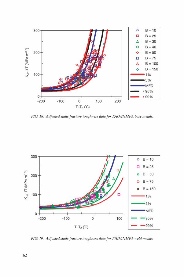
B = 10
B = 25
B = 30
B = 40
B = 50
B = 75
B = 100
B = 150
1%
5%
MED
95%
99%
300
200
100
0
T–T0 (˚C)
-200 -100 0 100 200
KJc
-1T
(MP
a·m
0.5 )
FIG. 18. Adjusted static fracture toughness data for 15Kh2NMFA base metals.
B = 10
B = 25
B = 50
B = 75
B = 150
1%
5%
MED
95%
99%
300
200
100
0-200 -100 0 100
T–T0 (˚C)
KJc
-1T
(MP
a·m
0.5 )
FIG. 19. Adjusted static fracture toughness data for 15Kh2NMFA weld metals.
62

7.7. RELATIONSHIP BETWEEN MARGIN (Y) AND TOLERANCE BOUND (X)
As previously discussed, the selection of the Master Curve lower tolerance bound (X) should be coupled with the selection of the margin term (Y).
As an exercise, using a CIEMAT literature review of fracture toughness data in the transition region2, a tentative relationship between X and Y was developed. Note that only the values within the –50°C £ T – T0 £ +50°C temperature region are used. The main details are summarized in Table 7.
The first exercise involved plotting the ASME KIC curve indexed to RTT0
without any margin relative to the fracture toughness data, which was followed by the determination of the Master Curve tolerance bound that bounds the same percentage of the data. As can be seen from Fig. 20, the 1.35% Master Curve tolerance bound and the ASME KIC curve indexed to T0 + 35ºF (19.4ºC) bounds 98.9% of the data. On the other hand, the Master Curve indexed to T0 + m, where m corresponds to a Y value of 3.55, also bounds the 98.9% of the data.
Following this process of assessing the X and Y values for Master Curve tolerance bounds (comparing with the Master Curve indexed to T0 + m), the same percentage of bounded data was established, creating the relationship between X and Y shown in Table 8.
TABLE 7. ESTIMATES OF UNCERTAINTIES [51]
ParameterUncertainty in
parameterUncertainty in
prediction
Copper content 0.1 mCu* wt% 11ºF (6ºC)
Nickel content 0.05 wt% 7ºF (4ºC)
Fluence 5ºF (3ºC) 7ºF (4ºC)
Irradiation temperature 10% 3ºF (2ºC)
T0, sT0 b/r1/2 18ºF (10ºC)
*mCu = median value of copper content (wt%).
2 CIEMAT Literature Review of Fracture Toughness Data in the Transition Region, internal report.
63

TABLE 8. RELATIONSHIP BETWEEN X AND Y
Y m(ºC)
X(%)
Data bounded (%)
1.49 19.44 5.55 92.6
2.00 26.11 3.65 95.5
2.71 35.37 2.55 97.5
3.00 39.16 2.00 98.1
3.55 46.34 1.35 98.9
400
350
300
250
200
150
100
50
0-60 -40 -20 0 20 40 60
T–T0 (ºC)
ASME KIC (RTT0 = T0+19.4) Master Curve tolerance bound X% = 1.35% Master Curve indexed to T0 + m (Y = 3.55)
Data bounded = 98.9%
FIG. 20. Comparison of X and Y.
64

7.8. MASTER CURVE SHAPE
Wallin [56] suggests that within the –50°C £ T – T0 £ +50°C temperature region, no remarkable deviations from the standard Master Curve shape occur.
A modified application of the Master Curve has been elaborated by Prometey and is presently utilized in the Russian Federation for RPV integrity assessment. Appendix III describes the Prometey probabilistic model for fracture toughness prediction. The intent of this modification is to clarify the applicability of the Master Curve to RPV steels having a high degree of embrittlement. The Prometey model provides a prediction of the KIC(T) curve allowing for the possibility of both a shift and a variation in shape for highly embrittled steels.
Figure 21 shows a comparison of the Prometey predictive model and the Master Curve for a WWER-1000 RPV base metal that has undergone special heat treatment (T41J = 180ºC).
It should be noted that Sokolov and Nanstad [25] suggest that irradiation does not necessarily alter the shape of the Master Curve, at least for DT41J up to 100ºC (see Fig. 22).
Similar results were obtained for irradiated WWER-440 RPV materials, as is shown in Fig. 23. It should be noted that five years’ irradiation of surveillance specimens represents fluence equal to approximately 3 × 1024 n/m2
(E > 0.5 MeV) [42].
-200 -150 -100 -50 0 50 100 150 200
300
200
100
0
B = 50 mmMaster Curve approach (T0 = 36.8ºC)
- test (2T-CT specimens with20% side grooves)
Pf = 0.5
Pf = 0.05
Pf = 0.95
KIC
, KJC
(MP
a·m
0.5 )
T (ºC)T (ºC)-200 -100 0 100 200
400
300
200
100
0
B = 50 mm- test (2T-CT specimens with20% side grooves)
Prometey model~sd = 4103 MPan = 12
KIC
, KJC
(MP
a·m
0.5 )
Pf = 0.95
Pf = 0.5
Pf = 0.05
(a) (b)
FIG. 21. Comparison of the predicted fracture toughness curves by (a) the Russian (Prometey) probabilistic model, and (b) the Master Curve approach (2Cr–Ni–Mo–V steel in embrittled condition).
65
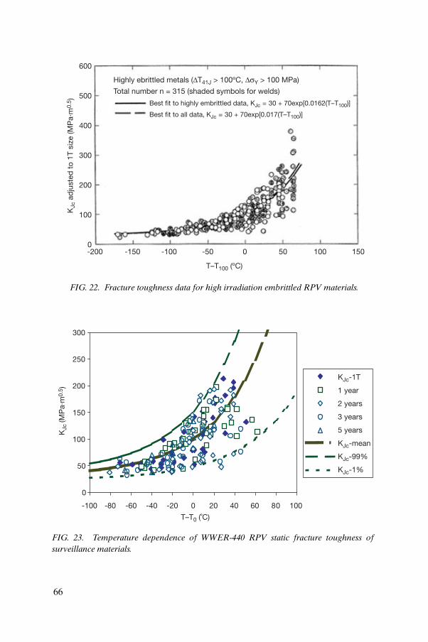
Highly ebrittled metals (DT41J > 100ºC, DsY > 100 MPa)
Total number n = 315 (shaded symbols for welds)
Best fit to highly embrittled data, KJc = 30 + 70exp[0.0162(T–T100)]
Best fit to all data, KJc = 30 + 70exp[0.017(T–T100)]
-200 -150 -100 -50 0 50 100 150
T–T100 (ºC)
600
500
400
300
200
100
0
KJc
ad
just
ed t
o 1T
siz
e (M
Pa·
m0.
5 )
FIG. 22. Fracture toughness data for high irradiation embrittled RPV materials.
0
50
100
150
200
250
300
-100 -80 -60 -40 -20 0 20 40 60 80 100
KJc
(MP
a·m
0.5 )
KJc-1T
1 year
2 years
3 years
5 years
KJc-mean
KJc-99%
KJc-1%
T–T0 (˚C)
FIG. 23. Temperature dependence of WWER-440 RPV static fracture toughness of surveillance materials.
66

8. PROBABILISTIC APPLICATION
The integrity of an RPV is determined by the capability of the structure to withstand transient loading without extending existing flaws through the structure. Fracture mechanics provides the technology for analysing the stability of an individual flaw under loads imposed by a particular transient. The loading on the large pressure retaining structures is analysed according to a linear elastic hypothesis and the behaviour of the flaw determined by the elastic stress intensity of the crack, KI (excluding underclad cracks). The material response to loading may be described by the critical stress intensity for crack initiation, KIC, and the arrest stress intensity for a running crack, KIa. If KIC and KIa are known, the response of an individual flaw to a known transient may be described.
An RPV integrity analysis must consider the flaw distribution (shape, location and density), the potential transients and the material properties.
8.1. POSSIBLE APPROACHES
There are two common approaches to this problem: deterministic and probabilistic.
In the deterministic approach, a limited number of fracture mechanics analyses are performed at the design stage using maximum flaw sizes, the most severe transient and lower bound toughness values. If vessel integrity can be demonstrated under these bounding conditions, integrity under all less severe conditions may be presumed.
Probabilistic analysis constitutes a significantly more robust analysis that includes the following elements:
(a) Estimation of flaw distribution (shape, location and density);(b) Characterization of the frequency and severity of all potential transients; (c) Evaluation of the uncertainty in the material toughness values and any
other input parameter that may be desired.
8.1.1. Flaws
Although RPVs are routinely inspected for flaws, integrity analysis must always include consideration of flaws that are below normal detection limits or which may have grown between inspection cycles (this is generally not a concern for practical application since no service induced crack growth is
67

expected). In most cases, vessel integrity will be limited by the behaviour of multiple postulated small flaws, including flaws that cannot be characterized by normal inspection techniques. Therefore, integrity analysis is generally based on a postulated flaw distribution.
8.1.2. Transients
There are numerous transients that could potentially challenge the integrity of the pressure vessel. The initiating event and subsequent reactions to that event will determine the severity and form of the transient loading. Although it is often possible to categorize transients in terms of their effect on the flaw tip stress intensity, the integrity of the vessel is generally dependent on the response to multiple possible transients.
8.1.3. Uncertainties in material toughness values
The primary material parameter controlling reactor vessel integrity is fracture toughness, KIC (or KIa). As already noted throughout this report, there are various possible sources of uncertainties in the material property definition, ranging from the availability of weld, heat affected zone or base sample material, and therefore size, type and number of specimens, to the effective transferability of the specimen results to RPV materials. Irradiation conditions (flux, temperature, fluence) and post-irradiation test parameters also introduce sources of uncertainty.
Fracture toughness is a strong function of temperature and an individual transient may present multiple temperatures. Therefore, the fracture toughness is generally described in terms of a characteristic toughness curve that defines the toughness as a function of temperature. The ASME reference toughness curve and the Master Curve are both characteristic toughness curves. Both curves require only the determination of a reference temperature (RTNDT or T0) to describe the material behaviour. However, the ASME reference toughness curve and the WWER design fracture toughness curves were originally developed to be used in deterministic analysis and describe a lower bound toughness value.
The Master Curve is more naturally suited to probabilistic analysis because it defines both a mean transition toughness value and a distribution around that value. Another aspect of the Master Curve approach is the crack length correction principle that is included in the methodology. Different manipulations of the ASME and WWER curves are required to obtain values to be used in a probabilistic analysis. Other, different databanks can be used to
68

derive these uncertainties on toughness values at a given location in a given vessel.
8.2. PROBABILISTIC ANALYSIS
In a probabilistic evaluation, the distributions mentioned are combined using Monte Carlo (or FORM–SORM) techniques to determine the probability of crack initiation and/or vessel failure. While the deterministic analysis can ensure reactor vessel integrity, it can be extremely conservative, especially if all the hypotheses, methods and data are chosen to be bounding.
A probabilistic analysis provides a more realistic evaluation of the vessel condition and corresponding safety level, incorporating all the available knowledge in the data and uncertainties in these data. Reactor vessel integrity may be ensured by setting limits on the allowable probability of failure. The use of a probabilistic approach allows a rational comparison to be made of RPV integrity with respect to other challenges to nuclear plant safety. Modern approaches to plant management can use probabilistic analysis to increase plant safety.
The Monte Carlo analysis used in a probabilistic fracture mechanics analysis requires multiple iterations to step through the various distributions of flaws, transients and material properties.
A schematic outline of the iterative loops required for a typical probabilistic fracture mechanics analysis is provided in Fig. 24. This schematic is based on the procedures developed at Oak Ridge National Laboratory and implemented in the FAVOR code; similar codes and procedures are available in other countries, e.g. France (OPERA code), Japan and Sweden.
In Fig. 24, a Master Curve based approach has been inserted in place of the RTNDT based approach used in the current version of the FAVOR code. Each RPV selected in the outer loop represents a single distribution of flaws through the volume of the reactor. Each flaw is analysed individually in the flaw loop. The flaw is characterized in terms of the reference temperature at the flaw location. The reference temperature is used to define the characteristic toughness versus temperature curve for the flaw.
The flaw response to a representative set of transients is then tested within the transient loop. Each transient can be characterized in terms of the load and temperature as a function of time. The probabilities of crack initiation and arrest are calculated as a function of time in the inner iteration loop.
69

The Monte Carlo simulation creates the matrix for the probability of failure as shown in Table 9.
Each vessel represents one sample from the combined flaw material parameter distribution. The sum over the transients (i) represents the probability of failure of each vessel (j). The histogram shown in Fig. 25 may be constructed to illustrate the distribution of vessel failure frequencies.
The overall frequency of failure can simply be represented as the sum over all trials:
RPV = RPV+1
flawj = flawj+1 Sample flaw
Sample material parameters
Calculate T0 at flaw tip
transient = transient +1
time = time +Dtime
Calculate aleatory failure frequency (@time)
CPIj = Maximum observed frequency
More time?
Crack growth
More transients?
More flaws?
Sum over flaws
More RPVs?
RP
V t
rial l
oop
Flaw
loop
Tran
sien
t lo
op
Tim
e lo
op
FIG. 24. Schematic of a probabilistic fracture mechanics analysis.
70
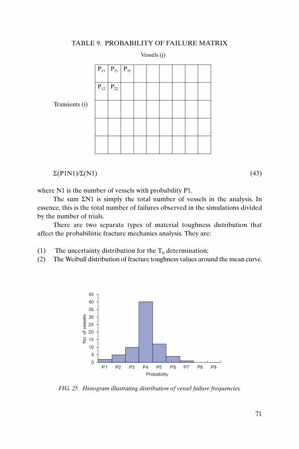
S(P1N1)/S(N1) (43)
where N1 is the number of vessels with probability P1.The sum SN1 is simply the total number of vessels in the analysis. In
essence, this is the total number of failures observed in the simulations divided by the number of trials.
There are two separate types of material toughness distribution that affect the probabilistic fracture mechanics analysis. They are:
(1) The uncertainty distribution for the T0 determination;(2) The Weibull distribution of fracture toughness values around the mean curve.
TABLE 9. PROBABILITY OF FAILURE MATRIX
Vessels (j)
P11 P21 P31
P12 P22
Transients (i)
0
5
10
15
20
25
30
35
40
45
P1 P2 P3 P4 P5 P6 P7 P8 P9
Probability
No.
of v
esse
ls
FIG. 25. Histogram illustrating distribution of vessel failure frequencies.
71

The uncertainty in the T0 determination is sometimes referred to as an epistemic uncertainty because it arises from a lack of knowledge about the material that could partially be eliminated if it were possible to make a more accurate measurement on the different material of a given vessel. At present, there are no available trend curves for determining the T0 value as a function of material composition and irradiation conditions. Therefore, T0 determinations can be based on measurements made on surveillance or other, similar, materials. There will be uncertainties associated with the measurements themselves as well as with the process of extending the surveillance material data to reflect all RPV operating conditions.
The procedures used to extend sample material measurements to the RPV are discussed in Section 5 of this report. These uncertainties can be used to construct a distribution of possible T0 values for the different flaw tip locations (weld, base metal, heat affected zone, top/bottom), as illustrated in Fig. 12. The T0 values used in the analysis must be selected from this distribution of possible values within the flaw loop. The number of RPV iterations included in the analysis must be sufficient to demonstrate that both the flaw distributions and the T0 distributions have been appropriately sampled.
The Master Curve describes a distribution of toughness values around a median toughness curve. The Weibull distribution in the Master Curve describes a variability that is inherent in the cleavage initiation mechanism of a homogeneous material. As this distribution reflects the stochastic nature of the process, which cannot be eliminated by better measurement, it is sometimes referred to as the aleatory portion of the uncertainty. The Master Curve Weibull distribution can be used to determine probability of failure, Pf, for applied stress intensity KIapp given material toughness KIC:
Pf(KIC < KIapp) = f(KIapp,T – T0) (44)
The basic fracture mechanics evaluation of flaw stability is equivalent to the evaluation applied to the limiting flaw in the deterministic evaluation. However, in the probabilistic analysis the probability of initiation must be evaluated at each time step in the transient (as indicated in Fig. 24). A cumulative probability of initiation is then calculated for each flaw in the vessel. In some analyses, the probability of an initiated flaw undergoing subsequent arrest is also considered on the ASME Section XI procedure basis, with a direct transfer of crack initiation Master Curve to crack arrest Master Curve.
Finally, the conditional probability of crack initiation and no crack arrest are estimated and compared with an acceptable risk level.
72

9. CONCLUSION
This publication has been written to allow utility engineers and scientists to measure directly fracture toughness using small surveillance-sized specimens and to apply the results using the Master Curve approach for RPV structural integrity assessment. The Master Curve methodology already has been or is being assimilated into the ASME Boiler and Pressure Vessel Code, ASTM standards, NRC regulations, German regulations (KTA 3203), the IAEA’s Guidelines on Pressurized Thermal Shock Analysis for WWER Nuclear Power Plants, as well as the VERLIFE Unified Procedure and other industry guidance documents governing RPV integrity analysis.
The general methodology adopted deals with both deterministic and probabilistic paths for assessing RPV structural integrity. The deterministic path is one that has been adopted by the ASME code in the USA using the reference temperature RTT0 as an alternative to RTNDT for indexing the ASME Code KIC curve. The German approach is essentially identical. The ongoing reassessment of the PTS screening criteria in the USA uses a probabilistic approach employing RTT0. Other application approaches that can be used are shown in Fig. 1. For WWER reactors, the Master Curve and the Prometey developed approach, which is similar to the Master Curve, are available options for the assessment of RPV integrity.
ASTM E 1921-02 is the basis for the fracture toughness testing and determination of T0 of the surveillance test sample. Adjustments to the measured value of T0 may be necessary to account for differences in the RPV material as compared with the surveillance material (i.e. they may not exactly match) and the neutron fluence (i.e. a functional relationship with fluence for interpolation or extrapolation is generally necessary).
It is reasonable to expect that in the future the determination of plant operating limits will be based on Master Curve methods. Under current codes and regulations, there are no specific requirements for Master Curve testing in RPV surveillance programmes. However, the need to assess more accurately RPV fracture toughness will drive some utilities to use modified surveillance specimens to measure Master Curve fracture toughness, in addition to undertaking traditional Charpy V-notch testing. For the vast majority of RPVs, significant margins against fracture can be demonstrated using current Charpy V-notch based methods. However, for plants that project significant embrittlement concerns during current or extended operating life, supplemental Master Curve testing may prove to be a critical, viable option. It is reasonable to expect increasing use of the Master Curve in RPV surveillance programmes and regulatory acceptance as experience with this technology continues to grow.
73


Appendix I
SINTAP FRACTURE TOUGHNESS ESTIMATION:ANALYSIS OF DATA FOR INITIATION OF BRITTLE FRACTURE
I.1. OVERVIEW
The MML method given below comprises three stages of analysis. Stage 1 gives an estimate of the median value of fracture toughness. Stage 2 performs a lower tail MML estimation, checking and correcting any undue influence of excessive values in the upper tail of the distribution. Stage 3 performs a minimum value estimation to check and make allowance for gross inhomogeneities in the material. In stage 3, an additional safety factor is incorporated for cases where the number of tests is small. The MML procedure produces reference values K0R and for, respectively, the 63.2% and 50% (median) cumulative failure probabilities from which a probability distribution can be calculated. The characteristic values are then obtained taking account of the factors. It is recommended that all three stages be employed when the number of tests to be analysed lies between 3 and 9. With an increasing number of tests, the influence of the penalty for small data sets is gradually reduced. For 10 or more tests, only stages 1 and 2 need be used. However, stage 3 may still be employed for indicative purposes, especially where there is evidence of gross inhomogeneity in the material (e.g. for weld or heat affected zone material). In such cases, it may be judged that the characteristic value is based upon the stage 3 result, or alternatively, such a result may be used as guidance in a sensitivity analysis.
The flow charts defining the major steps of the SINTAP analysis and the schematic drawings on data censoring are shown in Figs 26–32 (the procedures for single and multitemperature data are shown separately in Figs 26, 28 and 30). The basic equations (Eqs (45)–(50)) and the estimation equations (Eqs (51)–(55)) are given in Figs 33 and 34, respectively. Accuracy of the SINTAP procedure (steps 1 and 2) versus the number of specimens (N) is shown in Fig. 32.
I.2. PRELIMINARY STEPS
The preliminary steps, including data censoring and specimen size adjustment (see Fig. 33, Eq. (45)), shall be performed according to ASTM E 1921.
KR
75

STEP 1
Data used for MML estimate of T0 (KMAT)
Specimen measuringcapacity limit
P = 50%
Normal MML
KMAT
T (˚C)
Censoring
FIG. 26. Overview of the SINTAP procedure.
Failure mode = brittle fi di = 1 Failure mode brittle fi di = 0
SIZE ADJUSTMENT (Eq. (45))
Tests at single
temperature
STEP 2
T0 (Eq. (49)) K0, KMAT (Eqs (47, 51))
STEP 1: NORMAL MML ESTIMATION
KMATi = Klimit fiKMATi = Klimitdi = 0
CENSORING
YesNo
FIG. 27. Data censoring procedure in step 1.
76

KMAT
P = 50%
Lower tail MMLSTEP 2
T (˚C)
Censoring
Data used for MML estimateof T0 (KMAT)
FIG. 28. Flowchart of the step 2 procedure.
No Yes
NoNo
STEP 2: LOWER TAIL MML ESTIMATION
KCENSi = KMAT or
KCENSi = 30 + 70exp[0.019(Ti-T0)]
KMATi > KCENSi fi KMATi = KCENSidi=0
CENSORING
Tests at single
temperature
T0i (Eq. (52))
T0i £ T0i-1 YesT0 (steps 1+2)STEP 3
Yes
T0 (steps 1+2)
K0i ≥ K0i-1
K0i, KMATi (Eqs (47, 51))
FIG. 29. Data censoring procedure in step 2.
77

KMAT
Used onlywhenn < 10
STEP 3Minimum value estimate
T (°C)
Single data used forestimate of T0 (KMAT)
P = 50%
FIG. 30. Flowchart of the step 3 procedure.
No
No
STEP 3: MINIMUM VALUE ESTIMATION
YesTests
at single temperature
K0 (step 3) < 0.9 K0 (steps1+2) or
T0 (step 3) > 8˚̊C + T0 (steps1+2)
Yes
STEP 3 ESTIMATE
K0, KMAT (Eqs (47, 53))
STEP 1+2 ESTIMATE
T0 (Eq. (54))
KMAT(Pf, T, B) (Eqs (45, 46))
FIG. 31. Minimum value estimation in step 3.
78

1 10 1000.4
0.6
0.8
1.0
1.2
5%
25%
50%
75%
95%
ACCURACY OF STEP 1 AND 2 K0 ESTIMATES
N
K0es
t – K
min
K0
– K
min
FIG. 32. Accuracy of step 1 and 2 estimates (K0est–Kmin)/(K0–Kmin) as a function of the
number of specimens (homogeneous material).
BASIC EQUATIONS
KMAT25 = 20 MPa·m0.5 + (KMAT – 20 MPa·m0.5) B
25 mm( )
KMAT = 20 MPa·m0.5 + (K0R – 20MPa·m0.5)[–ln(1–Pf)]¼
K0 ª 31 + 77exp[0.019(T–T0)]
KMAT = 20 MPa·m0.5 + (K0 – 20 MPa·m0.5)(ln 2)¼
(45)
(46)
(47)
(48)
(49)
(50)
KMAT = 30 + 70exp[0.019(T–T0)]
FIG. 33. Basic equations (refer to flowcharts).
Pf = 1 – exp – ( )KMAT – 20 MPa·m0.5
K0 – 20 MPa·m0.5
4
79

I.3. SINTAP PROCEDURE
The procedure described hereinafter can be used both for single and multitemperature data.
I.3.1. Stage 1: MML estimation of T0
The value of T0 is calculated by an iterative process using the MML estimation method (Eq. (52) in Fig. 33 and Eq. (23) in ASTM E 1921-02).
I.3.2. Stage 2: Lower tail estimation
Establish TR as a reference value for T0 in the following way:
ESTIMATION EQUATIONS
FIG. 34. Estimation equations (refer to flowcharts).
)
,
(K MPa–
( )K MPaPa=K M
� MATi
N
ii
N
i
0
4
1
1
2020–
=
=
N 1 4
2
ln
/
( )T
NMPaMAT
i
i
0
1 4
202
11
77
00191
–
=
lnln
.
/
rTT KR
14+=
·m0.5·m0.5
��
Pa=K M0 20 ·m0.5 ( K MPaMATmin20–
·m0.5
�
·m0.5 ·m0.5
(51)
(53)
(54)
(55)
1 4/
,= max
+
+ ) (
( ))
iT
�����������������������
�����������������������
80

(a) Censor all data whose toughness, Ki, exceeds a value given by Eq. (49) in Fig. 33, setting di for the censored data equal to 0 and di for all other data equal to 1.
(b) Define the fracture toughness for these data as Ki = KT.(c) Establish a test value for T0, TT, following the procedures of stage 1
above. Compare the two values, T0 and TT. If TT is not greater than T0, term this value TK. If TT is greater than T0 repeat the exercise, using TT as a new benchmark for determining KT. Continue the iteration until a constant value of TT is obtained. Term this value TK.
(d) If the number of specimens in the data set is 10 or more (i.e. if n > 10), TK
= TR and determine K0R and from Eqs (48, 49). Use these values to determine the probability distribution and characteristic values. If the number of specimens in the data set is less than 10, perform MML stage 3 (minimum value) estimation, as described below.
I.3.3. Stage 3: Minimum value estimation
(a) Calculate the maximum value of T0, T0(max), using only non-censored data, i.e. where di = 1 and Eq. (54) in Fig. 34. Note that Ti is the test temperature of a specimen of toughness Ki and N is the total number of test results in the data.
(b) Compare T0(max) and TK. If T0(max) –8°C < TK, the data may be considered to be homogeneous and the value TK may be taken as representative. If T0(max) – 8°C > TK, this indicates that the data are inhomogeneous and T0(max) should be taken as the representative value. Term this value TK.
(c) Determine reference values including any necessary safety correction for a small data set. Use Eq. (55) (Fig. 34) to calculate the final values of T0
and TR for determination of reference values of toughness according to (d), below. Note that r is the number of specimens in the data set which failed by a brittle mechanism.
(d) Calculate both and K0R as a function of temperature, T, using Eqs (48, 49) in Fig. 33.
I.4. DETERMINATION OF CHARACTERISTIC VALUES
(a) Calculate the statistical distribution, P{KMAT}, from Eq. (46) (Fig. 33). For data over a range of temperatures, these may be calculated at any appropriate temperature.
(b) Determine the characteristic value KMAT. Equation (50) can be used to give a characteristic value for the toughness in terms of KMAT as a
KR
KR
81

function of the probability failure, Pf, and the value of K0 obtained. Equation (47) can be used for Pf = 0.5.
In using Eq. (50), the following factors need to be considered: (1) the reliability of the result needed, which will determine the choice of Pf (e.g. 0.05 or 0.02), and (2) the importance of the stage 3 result for data sets above 10, which will determine what value of K0 is used.
82

Appendix II
EXAMPLES OF ABNORMAL FRACTURE TOUGHNESS DATA ASSESSMENT
II.1. EXAMPLES: SINTAP APPLICATION
An example of the SINTAP application is shown in Fig. 35. Figure 35(a) shows the standard Master Curve approach as applied to several welds subjected to different irradiation conditions. The SINTAP application is shown in Fig. 35(b). The value of T0 increased in the SINTAP estimation from 33oC to 59oC.
1%5%
95 %
5%
Trawsfynydd Weld sY = 400 MPa B = 10 mm
M = 30
T (˚C)-100 -50 0 50 100 150 200
200
150
100
50
0
KJc
(MP
a·m
0.5 )
95%CLEAVAGE DUCTILE T0 = 33˚C B0 = 25 mm
T (˚C)-100 -50 0 50 100 150 200
Trawsfynydd Weld sY = 400 MPa B = 10 mm
200
150
100
50
0
KJc
(MP
a·m
0.5 )
(a)
(b)
M = 30
CLEAVAGE DUCTILE T0 = 59˚C B0 = 25 mm
FIG. 35. Application of (a) the standard Master Curve approach, and (b) the SINTAP procedure to adjust the lower bound estimation of an inhomogeneous data set.
83

II.2. MASTER CURVE AND GRAIN BOUNDARY FRACTURE
Grain boundary fracture may affect the fracture behaviour in or near the transition range and thus the applicability of the Master Curve method. Its occurrence is often revealed by exceptionally low fracture toughness values below or above the temperature range T0 ± 50oC. The effect of grain boundary fracture is clarified in the following examples for steels A533B, A508 and A302B tested in as-received (unembrittled) or thermally aged conditions (Figs 36–40) as taken from Refs [52–54].
The effect of grain boundary fracture on the fracture behaviour depends on (1) the proportion of grain boundary fracture, and (2) the temperature range in respect of T0. In the lower shelf area, even if fracture occurs predominantly by a transgranular mode, the Master Curve analysis can usually be performed successfully by reducing Kmin from the normally assumed constant value of 20 MPa·m0.5. Examples of data which follow the Master Curve at low temperatures (below T0 – 50ºC),despite the 100% incidence of grain boundary fracture, are shown in Figs 37 and 39. Thus, it may be possible to apply the Master Curve below T0 – 50ºC in such cases. An example of a poor correspondence at high temperatures is shown in Fig. 40.
(a)
5%
95% T0 = -58˚C B0 = 25 mm
(b)
5%
95%
T (˚C)
200
150
100
50
0
M = 30 M = 30
-200 -150 -100 -50-200 -150 -100 -50 0
KJc
(MP
a·m
0.5 )
KJc
(MP
a·m
0.5 )
200
150
100
50
0
A533B CI.1 sY = 485 MPa B = 12.5 mm REFERENCEA533B CI.1 sY = 485 MPa B = 12.5 mm REFERENCE
T (˚C)
CLEAVAGE DUCTILE T0 = -62˚C B0 = 25 mm K0 = 15 + 93×exp[0.019(T-T0)] Kmin = 10 MPa·m0·5
CLEAVAGEDUCTILE
FIG. 36. Master Curve analysis of data measured for unembrittled A533B Cl. 1 steel: (a) standard Master Curve analysis, (b) lower shelf modified Master Curve analysis [52].
84
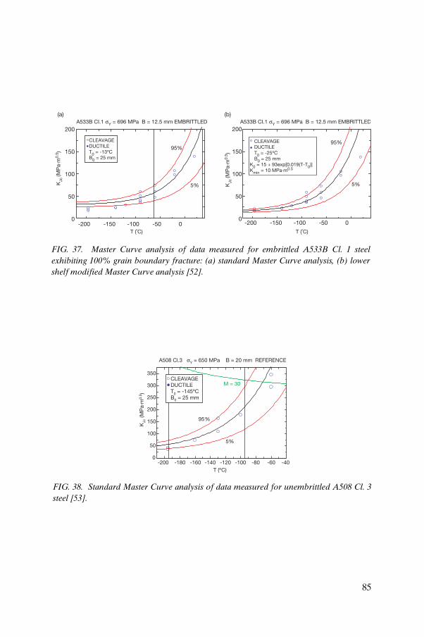
CLEAVAGE DUCTILE T0 = -13ºC B0 = 25 mm
CLEAVAGE DUCTILE T0 = -25ºC B0 = 25 mm K0 = 15 + 93exp[0.019(T-T0)] Kmin = 10 MPa·m0.5
5%
95%
5%
95%
T (˚C)
KJc
(MP
a·m
0.5 )
200
150
100
50
0
T (˚C)
A533B CI.1 sY = 696 MPa B = 12.5 mm EMBRITTLED A533B CI.1 sY = 696 MPa B = 12.5 mm EMBRITTLED
KJc
(MP
a·m
0.5 )
-200 -150 -100 -50 0-200 -150 -100 -50 0
200
150
100
50
0
(a) (b)
FIG. 37. Master Curve analysis of data measured for embrittled A533B Cl. 1 steel exhibiting 100% grain boundary fracture: (a) standard Master Curve analysis, (b) lower shelf modified Master Curve analysis [52].
0
50
100
150
200
250
300
350
5%
95 %
A508 Cl.3 sY = 650 MPa B = 20 mm REFERENCE
T (ºC)
M = 30
-200 -180 -160 -140 -120 -100 -80 -60 -40
KJc
(MP
a··m
0.5 )
CLEAVAGE DUCTILE T0 = -145ºC B0 = 25 mm
FIG. 38. Standard Master Curve analysis of data measured for unembrittled A508 Cl. 3 steel [53].
85

0
50
100
150
200
250
300
5%
95 %
0
50
100
150
200
250
300
5%
95%
A508 Cl.3 sY = 560 MPa B = 20 mm EMBRITTLED
CLEAVAGE DUCTILE T0 = -45ºC B0 = 25 mm
T (ºC)-200 -150 -100 -50 0
M = 30
A508 Cl.3 sY = 560 MPa B = 20 mm EMBRITTLED
M = 30
T (ºC)-200 -150 -100 -50 0
CLEAVAGE DUCTILE T0 = -48ºC B0 = 25 mmK0 = 17 + 91exp[0.019(T-T0)]Kmin = 10 MPa·m0.5
KJc
(MP
a··m
0.5 )
KJc
(MP
a··m
0.5 )
(a) (b)
FIG. 39. Master Curve Analysis of data measured for embrittled A508 Cl. 3 steel exhibiting 100% grain boundary fracture: (a) standard Master Curve analysis, (b) lower shelf modified Master Curve analysis [53].
0
50
100
150
200
250
300
5%
95%
0
50
100
150
200
250
300
350
a = 1 mm
5%
95%
M = 30
T (ºC)
-150 -100 -50 0
KJc
(MP
a··m
0.5 )
KJc
(MP
a··m
0.5 )
A302 B mod sY = 472 MPa B = 12.5 mm UNAGED A302 B mod sY = 472 MPa B = 12.5-50 mm AGED
T (ºC)
-150 -100 -50 0 50 100
CLEAVAGE DUCTILE T0 = -139ºC B0 = 25 mm
(a) (b)
CLEAVAGE DUCTILE T0 = -96ºC B0 = 25 mm
Da = 0.2 mm
FIG. 40. Master Curve analysis of data measured for modified A302B steel in (a) unembrittled and (b) embrittled (showing 95% grain boundary fracture) conditions [54].
86

II.3. EXAMPLES: APPLICATION OF THE MASTER CURVE OUTSIDE THE –50°C ≤ T – T0 ≤ +50°C RANGE
II.3.1. General principle
An integrity assessment based on the Master Curve analysis should primarily be limited within the temperature range –50°C £ T – T0 £ +50°C [5]. If this is not possible, the assessment should be based on test data measured at temperature(s) as close as possible to the assessment temperature. If such fracture toughness data exist and indicate ‘normal’ fracture behaviour following the Master Curve prediction, or if the material is known to be homogeneous and exhibits such a fracture behaviour at the assessment temperature, outside the valid temperature range, then the Master Curve can be extrapolated in the basic form without adjusting the estimation.
II.3.2. Application near the lower shelf
In the low temperature region, the standard Master Curve distribution normally gives a conservative estimate. If sufficient data exist, the lower shelf prediction can be fitted by estimating the minimum fracture toughness, normally set as 20 MPa·m0.5 (described below). Usually, no size adjustment is needed in or near the lower shelf region or the effect of the adjustment is insignificant. If more than one initiation site exists on the specimen fracture surface, there is usually no need for size adjustment. When approaching the lower shelf there is decreasing benefit from constraint considerations.
II.3.3. Application near the upper shelf
The data measured in the high temperature region should be checked for ductile crack growth and constraint effects. The censoring procedure should be applied for test results where no brittle crack initiation has occurred or where stable crack growth prior to cleavage initiation is large with respect to specimen size (the validity criteria specified in ASTM E 1921 should be used for comparison).
Crack growth effects can be considered conservatively by applying the SINTAP lower tail procedure. Empirical crack size adjustment is required to apply the high temperature data (often sufficient to consider the high constraint region).
Figure 41 shows examples of the Master Curve analysis performed for a weld metal in the as-received (a) and irradiated (b–d) conditions. In all conditions the data follow the standard Master Curve both within the valid
87

temperature range (a–c) and below it (a and c). The difference between the 1T and ½T specimen results (b) may be caused by material inhomogeneity. The lower bound was therefore adjusted by applying the SINTAP procedure (d).
II.3.4. Lower shelf adjustment: Background
The Master Curve model includes an assumption for the minimum fracture toughness, Kmin, which is achieved as the temperature approaches the lower shelf of KJc. In the basic model (ASTM E 1921), the Kmin has a constant value (20 MPa·m0.5), independent of the material. This value has been defined empirically and found to give a lower shelf fit suitable for most ferritic steels.
-100 -50 0 50 100 1500
50
100
150
200
250
300
5 %
95 %
100 150 200 2500
50
100
150
200
250
300
5 %
95 %
0 50 100 150 200 250 3000
50
100
150
200
5 %
95 %
120 140 160 180 200 220 240 2600
50
100
150
200
250
300
350
5 %
95 %
(a) (b)
(c) (d)
KS01 SG REF. sY = 600 MPa B = 12.5–50 mm KS01 SG f f = 0.84 sY = 820 MPa B = 12.5 and 25 mm
MPA ORNL CLEAVAGE ORNL DUCTILE T0 = -28ºC B0 = 25 mm
KJc
(MP
a·m
0.5 )
KJc
(MP
a·m
0.5 )
CLEAVAGE DUCTILE T0 = 133ºC B0 = 25 mm ½T
KS01 SG f f = 0.84 sY = 820 MPa B = 12.5 and 25 mm KS01 SG f f = 8.40 sY = 950 MPa B = 25-50 mm
SINTAP analysis
T – T0 (ºC) T (ºC)
T (ºC)T (ºC)
CLEAVAGE DUCTILE T0 = 271ºC B0 = 25 mm
KJc
(MP
a·m
0.5 )
KJc
(MP
a·m
0.5 )
CLEAVAGE DUCTILE T0 = 148ºC B0 = 25 mm
FIG. 41. Test data for MPA weld KS01 which illustrates the sample’s extreme sensitivity to irradiation: (a) is as-received, (b–d) in irradiated condition. Within the range –50°C £ T – T0 £ +50°C the values follow the standard Master Curve (a–c). The difference between the 1T and ½T specimen results (b) may be caused by material inhomogeneity. The application of the SINTAP procedure is shown in (d).
88

Theoretically, Kmin values between 10 MPa·m0.5 and 35 MPa·m0.5 may be possible. There is generally, however, no need to estimate a material specific lower shelf toughness for structural steels.
In certain cases, the lower shelf behaviour may deviate from that predicted to an extent that it is also necessary to estimate Kmin to improve the fit in the lower shelf region. Typically, the deviation results from the lower than predicted lower shelf level which is often associated with large proportions of fracture mode(s) other than pure cleavage. Such situations have been encountered with steels susceptible to temper embrittlement that have undergone thermal ageing in the critical temperature area and/or neutron irradiation to a high fluence.
A modified Master Curve procedure, based on the multitemperature model, has been introduced for analysing fracture toughness data showing exceptional lower shelf behaviour [55]. In this model, the lower shelf value is not given as a constant value but as a variable, to be adjusted to give the best estimate fit in the lower shelf area. As a result of a proper lower shelf fit this procedure also often improves the overall consistency of the measured and predicted data.
The application of, and equations for, the lower shelf adjustment are discussed in the following section. Examples of applying the method, showing the effect of the adjustment, are given in the above examples discussing the grain boundary fracture cases and extrapolation.
II.3.5. Lower shelf adjustment: Application
Close to the lower shelf fracture toughness (KIC < 50 MPa·m0.5), the basic Master Curve equations are expected to be inaccurate. The model is based upon the assumption that brittle fracture is primarily initiation controlled, even though it contains a conditional crack propagation criterion, which, among other factors, is the cause of the lower bound fracture toughness Kmin. On the lower shelf, the initiation criterion is no longer dominant, but the fracture is completely propagation controlled. In this case there is no statistical size effect and the toughness distribution also differs, albeit slightly, from the standard one. In the transition region the basic equations should be valid as long as loss of constraint and/or ductile tearing do not play a significant role.
The modified method improves the lower shelf accuracy and is more material specific. The Master Curve is modified for the lower shelf by fitting the athermal part of the Master Curve to the lower shelf data as follows:
(56)
where a is a fit constant.
K a a T T0 = exp .+ -( ) -( )ÈÎ ˘̊108 0 019 0
89

In this way the material specific lower shelf range can be correctly taken into account without significantly changing the properties of the Master Curve in the transition region. The constants a and T0 are determined by the MML method as follows [55]:
(57)
(58)
Equations (57) and (58) are solved iteratively to enable determination of a and T0. If there is an indication of Kmin being less than 20 MPa·m0.5, this can be adjusted from the equations as well.
i i 0
i 0
exp . T T
a exp . T
d 0 019 1
20 108 0 0191
-( )ÈÎ ˘̊ -
- + -( ) -( )ÈÎ ˘̊= a Ti
n
ÂÂ
--( ) -( )ÈÎ ˘̊ -{ }
- -( )
K exp . T T
a + exp .
iIC i 020 0 019 1
20 108 0 019
4
a ii 0T T = 0
-( )ÈÎ ˘̊{ }=Â 5
1i
n
i i 0
i 0
exp . T T
a exp . T T
d 0 019
20 108 0 019
-( )ÈÎ ˘̊
- + -( ) -( )ÈÎ ˘̊=Â ai 1
n
K exp . T T
a + exp . T T
iIC i 0
i 0
--( ) -( )ÈÎ ˘̊
- -( ) -(20 0 019
20 108 0 019
4
a ))ÈÎ ˘̊{ }=Â 5i 1
n
= 0
90

Appendix III
PROMETEY PROBABILISTIC MODEL FOR FRACTURE TOUGHNESS PREDICTION
The Master Curve concept utilizes a constant curve shape that is indexed using the reference temperature, T0. The reference temperature, T0, can also be used to index the ASME code KIC curve for unirradiated and irradiated RPV steels [7]. There is some concern that for highly embrittled materials, the shapes of the KIC(T) curves may change [56, 57]. Utilizing a constant curve shape for these cases may lead to a non-conservative estimate of fracture toughness. In such cases it is necessary to define the conditions when a constant curve shape is not appropriate.
Conditions for application of the Master Curve are based on the concept of cleavage fracture. There also exist several models based on the local approach to fracture [58–60]. These include the RKR model [59, 60] and the Beremin model [61]. However, it has been shown [15, 62] that fracture toughness prediction of irradiated RPV steels using the RKR and Beremin models does not fully describe the experimental data. According to the RKR and Beremin models, the temperature dependence of fracture toughness, KIC(T), is determined by the temperature dependence of the yield stress sY(T). For RPV steels over the temperature range 20oC £ T £ 300oC, the yield stress varies very weakly. For RPV steels with large values of transition temperature (e.g. irradiated steel), the increase in KIC with temperature is predicted to be small, in contrast with experimental data [15, 63].
The Prometey model for fracture toughness prediction is based on a new formulation of the local cleavage fracture criterion [64, 65] in both a deterministic [64, 66] and a probabilistic [67–69] manner. The probabilistic model was verified by application to RPV steels for WWER-440 and WWER-1000 units in both initial and embrittled states [56, 57, 62, 67–69].
It should be noted that the Prometey model discussed in Refs [67–69] does not include any assumptions concerning the shape of the KIC(T) curve or the temperature shift condition but provides a prediction of the KIC(T) curve, allowing for the possibility of both a shift and a variation of curve shape.
Appendix III describes the formulation of the local cleavage fracture criterion in a probabilistic manner, the Prometey probabilistic model for predicting the KIC(T) curve and methods for the experimental determination of the necessary parameters.
91

III.1. THE LOCAL CRITERION FOR CLEAVAGE FRACTURE
The formulation of the local cleavage fracture criterion in a probabilistic manner is described in the following six steps [64, 65, 67].
Step 1. The polycrystalline material is viewed as an aggregate of cubic unit cells. The mechanical properties of each unit cell are taken as the average properties obtained by standard specimen testing. The size of the unit cell (ruc) is never less than the average grain size. The stress and strain fields in the unit cell are assumed to be homogeneous.
Step 2. The local criterion for cleavage fracture of a unit cell is taken as [64, 65]:
s1 + mTεseff ≥ sd (59)
s1 ≥ SC(æ) (60)
where the critical brittle fracture stress, SC(æ), is calculated from:
SC(æ) = [C*1 + C*
2 exp(–Ad)]–1/2 (61)
where
s1 is the maximum principal stress;seff = seq–sY is the effective stress.;seq is the equivalent stress;sY is the yield stress;
æ is Odqvist’s parameter;
is the equivalent plastic strain increment;C1
*, C2*, Ad are material constants;
sd is the strength of carbides or ‘carbide–matrix’ interfaces or other particles on which cleavage microcracks are nucleated;
mTε is a parameter that depends on temperature (T) and plastic strain and may be written [67, 69] as:
mTε = mT(T)mε(æ) (62)
mε(æ) = S0/SC(æ) (63)
mT(T) = m0sYs(T) (64)
= Ú deeqp
d eqpe
92
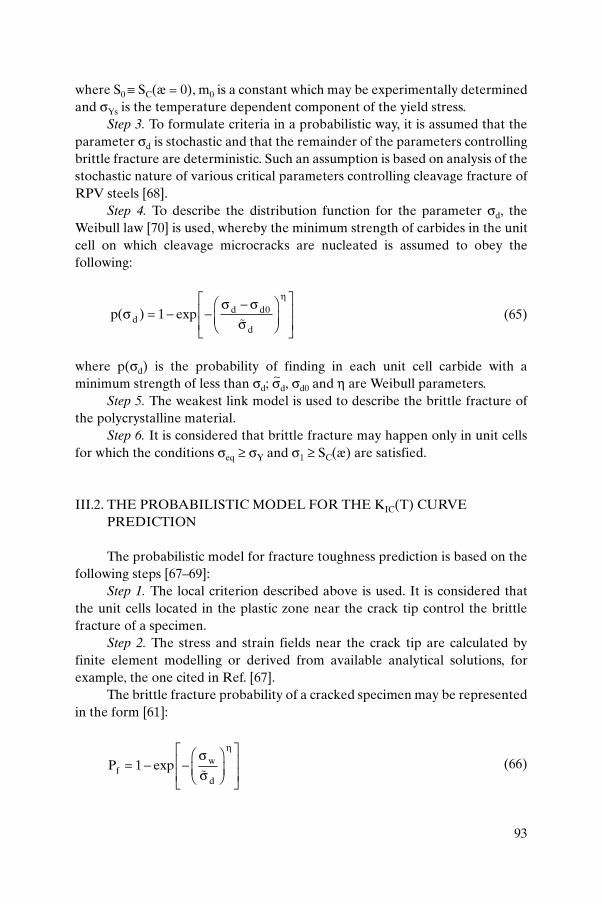
where S0 ∫ SC(æ = 0), m0 is a constant which may be experimentally determined and sYs is the temperature dependent component of the yield stress.
Step 3. To formulate criteria in a probabilistic way, it is assumed that the parameter sd is stochastic and that the remainder of the parameters controlling brittle fracture are deterministic. Such an assumption is based on analysis of the stochastic nature of various critical parameters controlling cleavage fracture of RPV steels [68].
Step 4. To describe the distribution function for the parameter sd, the Weibull law [70] is used, whereby the minimum strength of carbides in the unit cell on which cleavage microcracks are nucleated is assumed to obey the following:
(65)
where p(sd) is the probability of finding in each unit cell carbide with a minimum strength of less than sd; s~d, sd0 and h are Weibull parameters.
Step 5. The weakest link model is used to describe the brittle fracture of the polycrystalline material.
Step 6. It is considered that brittle fracture may happen only in unit cells for which the conditions seq ≥ sY and s1 ≥ SC(æ) are satisfied.
III.2. THE PROBABILISTIC MODEL FOR THE KIC(T) CURVE PREDICTION
The probabilistic model for fracture toughness prediction is based on the following steps [67–69]:
Step 1. The local criterion described above is used. It is considered that the unit cells located in the plastic zone near the crack tip control the brittle fracture of a specimen.
Step 2. The stress and strain fields near the crack tip are calculated by finite element modelling or derived from available analytical solutions, for example, the one cited in Ref. [67].
The brittle fracture probability of a cracked specimen may be represented in the form [61]:
(66)
p dd d
d
( ) expss s
s
h
= - --Ê
ËÁˆ
¯̃
È
ÎÍÍ
˘
˚˙˙
1 0
�
Pfw
d
= - -Ê
ËÁˆ
¯̃
È
ÎÍÍ
˘
˚˙˙
1 expss
h
�
93

where the Weibull stress, sw, is:
(67)
where
In Eq. (67), k is the number of unit cells in the plastic zone, i is the number of a unit cell, for ith unit cell, the parameter m(si
nuc) is the maximum value of the parameter si
nuc for this unit cell over the whole loading history from the beginning to the current moment. The above equations allow the calculation of the dependence of the brittle fracture probability on the stress intensity coefficient, Pf(KI), as the parameter sw is a function of KI.
III.3. EXPERIMENTAL DETERMINATION OF PARAMETERS NECESSARY FOR BRITTLE FRACTURE TOUGHNESS PREDICTION
To describe the KIC(T) curve on the basis of the model proposed, it is necessary to know the parameters SC(æ), mT(T), s~d, sd0 and h and also parameters describing plastic deformation to enable the stress and strain fields to be calculated.
The stress–strain curve is approximated by:
(æ)n (68)
where A0 and n are material constants. The temperature dependence of the yield stress sY(T) is approximated by:
(69)
where a, b, c and h are material constants independent of temperature and T is the temperature in kelvin.
For pressure vessel steels, Eq. (69) with c = 0 describes experimental data well over the low to moderate (up to 50oC) temperature range [62, 67, 69]. Equation (69) appears to be a good approximation of the dependence sY(T) over the low and elevated (up to 450oC) temperature range [62].
s s sh
h
w nuci
di
k
= -( )È
ÎÍÍ
˘
˚˙˙=
 max( )
/
01
1
ss s s s s
s se
nuci
iT eff
i iC i nuc
id0
d
m m , if S ) and
, if ∫
+ ≥ >1 1
0 1
(ii
C i nuci
d0S ) or < £
ÏÌÔ
ÓÔ ( s s
æ
æ
s seq Y A= + 0
s Y (T) a cT b[exp( hT)]= - + -
94

The constants in Eqs (61), (68) and (69) are determined from the results of testing standard tensile specimens at various temperatures [65]. The parameter mT(T) is calculated from Eq. (65). The parameter m0 may be found by the procedure presented in Ref. [67]. The temperature dependent component, sYs(T), is determined from:
(70)
where sYG, the temperature independent component, may be taken as the value of the yield stress (sY) at some temperature TYG for which sYs(TYG) < 0.01sY(TYG). For RPV steels, TYG may be taken to be 350oC [62, 67, 69].
The parameters s~d and h may be determined from the results of testing small-sized fracture toughness specimens at one temperature, similar to the single temperature option of the Master Curve.
The parameter sd0 may be estimated as the minimum possible value of the parameter sd with the microcrack nucleation condition (Eq. (59)) if it is assumed that microcracks may be nucleated at seq = sY at a temperature close to absolute zero. For this case, seff = 0 and s1 ª sY, so that it follows from Eq. (59) that sd0 ª sY and from Eq. (68) sY ª a + b leading to sd0 ª a + b.
The procedure for determination of s~d and h, assuming that the parameter m0 is known, is as follows:
(1) Small-sized fracture toughness specimens are tested at temperature T and values of KJc are determined.
(2) Stress and strain fields for each cracked specimen are calculated.(3) Some initial value of h = h0 is taken. (4) Values of sw for each cracked specimen are calculated using Eq. (67) and
incorporating the values for the stress and strain fields obtained from (2) above.
(5) The parameters s~d and h in Eq. (66) are determined by the MML method.
(6) The values of h and h0 are compared:if h ª h0 then the iterative process is interrupted;if h π h0 then the value of parameter h0 is corrected and the process is repeated according to steps 4–6.
Thus, the parameters of the probabilistic model are determined by using test results from standard tensile specimens at various temperatures and small-sized fracture toughness specimens at one temperature.
s s sYs Y YG(T) = (T) -
95

Appendix IV
LIST OF ABBREVIATIONS AND SYMBOLS
D temperature margin (°C)
DRT irradiation induced shift of Charpy or fracture toughness (°C)
DT41J Charpy 41J transition temperature shift (°C)
DT100 reference fracture toughness temperature shift at 100 MPa·m0.5 (°C)
DTCVN Charpy transition temperature shift (°C)
DT0 Master Curve reference temperature shift (°C)
FRPV, FSM irradiation conditions for RPV and sample materials
[n] Poisson’s ratio for steel (0.3)
[s] allowable stress in WWER RPVs (MPa)
sCu uncertainty in copper content (wt%)
sHT uncertainty due to material heat treatment (non-homogeneity) (°C)
sI uncertainty in material initial condition (°C)
sMC uncertainty due to material condition (variability) (°C)
sNi uncertainty in nickel content (wt%)
sProj uncertainty due to projection to higher fluence (°C)
sTirr uncertainty due to irradiation temperature (°C)
sT0 uncertainty in reference temperature T0 (°C)
sys yield strength (MPa)
s∆ uncertainty in Charpy shift (°C)sφt uncertainty in neutron fluence (°C)
CRPV, CSM material composition for RPV and sample materials
¼-T one quarter of the wall thickness (mm)
¾-T three quarters of the wall thickness (mm)
a characteristic value of the crack depth (smaller semi-axis) (mm)
ART adjusted reference temperature
B1T thickness B = 1T (25.4 mm)
B0 thickness of the tested specimen (side grooves not considered) (mm)
96

CFCVN chemistry factor for the Charpy 41J temperature shift (°C)
CFT0 chemistry factor for the fracture toughness shift (°C)
E Young’s modulus (GPa)
E > 0.5 MeV neutron energies greater than 0.5 MeV
E > 1 MeV neutron energies greater than 1 MeV
f neutron fluence (n/m2)
fsurf neutron fluence on inner surface of RPV (n/m2)
Jc critical value of the J-integral
Je elastic component of the J-integral
Jp plastic component of the J-integral
KI applied stress intensity factor (MPa·m0.5)
KIa crack arrest fracture toughness (MPa·m0.5)
KIC plane strain crack initiation reference fracture toughness (MPa·m0.5)
KIR crack arrest reference fracture toughness (MPa·m0.5)
KJc plain strain cleavage fracture toughness (MPa·m0.5)
KJc(0.xx) lower and upper tolerance bound for the estimated fracture toughness (MPa·m0.5)
KJc(limit) validity limit for measured KJc (MPa·m0.5)
Kmin lower bound fracture toughness fixed at 20 MPa·m0.5 in ASTM E 1921-02
Pf failure probability
RTNDT reference transition temperature (°C) as per ASME code
RTT0 reference transition temperature based on Master Curve (°C)
RTT0(I) initial reference temperature RTT0 (°C)
T test temperature (°C)
T41J transition temperature measured at Charpy energy of 41J (°C)
TCVN Charpy V-notch transition temperature corresponding to a 28J or 41J Charpy V-notch impact energy (°C)
TF final transition temperature for WWER RPVs (°C)
Tk transition temperature based on Charpy tests for WWER reactors (°C)
97

Tk0 initial transition temperature based on Charpy tests for WWER reactors (°C)
Tka maximum allowable transition temperature of WWER RPVs during
PTS (°C)
T0 Master Curve reference temperature (°C) as per ASTM E 1921
Y added safety (comfort) parameter in the margin term
Kcen censored value of toughness in units of K
di censoring parameter
Ki individual values of fracture toughness adjusted to 25 mm thickness
Kmin minimum value of Ki
N number of specimens in data set
r number of valid and uncensored KJc test values in the data set that fail by brittle cleavage fracture
K0 63.2% cumulative failure probability
m median value (50% cumulative failure probability)
K0(min) minimum value of K0
T test value of m for MML stage 2
K constant value of m derived from MML stage 2
K0K value of K0 associated with K
K0R reference value of K0
R reference value of m
t section thickness or wall thickness of RPV
Ti test temperature of specimen of toughness Ki
T0 transition temperature corresponding to median at toughness of 100 MPa·m0.5
TR reference value of T0
TT test value of T0
TK constant value of T0 obtained from MML stage 2
T0(max) maximum value of T0
P{KMAT} probability distribution
K
K K
K K
K
K K
98

REFERENCES
[1] INTERNATIONAL ATOMIC ENERGY AGENCY, Co-ordinated Research Programme on Irradiation Embrittlement of Pressure Vessel Steels, Rep. IAEA-176, IAEA, Vienna (1975).
[2] INTERNATIONAL ATOMIC ENERGY AGENCY, Analysis of the Behaviour of Advanced Reactor Pressure Vessel Steels under Neutron Irradiation, Technical Reports Series No. 265, IAEA, Vienna (1986).
[3] INTERNATIONAL ATOMIC ENERGY AGENCY, Reference Manual on the IAEA JRQ Correlation Monitor Steel for Irradiation Damage Studies, IAEA-TECDOC-1230, IAEA, Vienna (2001).
[4] WALLIN, K., The scatter in KIc results, Eng. Fract. Mech. 19 (1984) 1085–1093.[5] AMERICAN SOCIETY FOR TESTING AND MATERIALS, Test Method for
Determination of Reference Temperature, T0, for Ferritic Steels in the Transition Range, ASTM-E-1921-02, ASTM, West Conshohocken, PA (2002).
[6] SERVER, W.L., et al., “Application of Master Curve fracture toughness for reactor pressure vessel integrity assessment in the USA”, paper presented IAEA Specialists Meeting on Irradiation Embrittlement and Mitigation, Gloucester, UK 2001.
[7] AMERICAN SOCIETY OF MECHANICAL ENGINEERS, Use of Fracture Toughness Test Data to Establish Reference Temperature for Pressure Retaining Materials, Section XI, Division 1, ASME Boiler and Pressure Vessel Code Case N-629, ASME, New York (1999).
[8] LOTT, R.G., et al., “Determination of margins and heat adjustments for Master Curve applications in RPV integrity analysis”, ASME Pressure Vessel and Piping (Proc. Symp. Seattle, 2000), American Society of Mechanical Engineers, New York(2000).
[9] LOTT, R.G., ROSINSKI, S.T., SERVER, W.L., “The technical foundations of a unified adjusted reference temperature for RPV fracture toughness”, Effects of Radiation on Materials (Proc. 21st Int. Symp. Tucson, 2002), American Society for Testing and Materials, West Conshohocken, PA (2002).
[10] NUCLEAR REGULATORY COMMISSION, Radiation Embrittlement of Reactor Vessel Materials, Rep. R.G. 1.99 Rev. 2, Office of Nuclear Regulatory Research, NRC, Washington, DC (1998).
[11] KIRK, M., LOTT, R.G., KIM, C., SERVER, W.L., “Empirical validation of the Master Curve for irradiated and unirradiated reactor pressure vessel steels”, ASME Pressure Vessel and Piping (Proc. Symp. San Diego, 1998), American Society of Mechanical Engineers, New York (1998).
[12] ROSINSKI, S.T., SERVER, W.L., LOTT, R.G., “A mechanistically-guided Charpy embrittlement correlation for RPV integrity assessment”, Effects of Radiation on Materials (Proc. 21st Int. Symp. Tucson, 2002), American Society for Testing and Materials, West Conshohocken, PA (2002).
99

[13] ENGLISH, C.A., SERVER, W.L., ROSINSKI, S.T., “Critical review of through-wall attenuation of mechanical properties in RPV steels”, Effects of Radiation on Materials (Proc. 21st Int. Symp. Tucson, 2002), American Society for Testing and Materials, West Conshohocken, PA (2002).
[14] KIRK, M., et al., Technical Basis for Revision of the Pressurized Thermal Shock (PTS) Screening Criteria in the PTS Rule (10CFR50.61), draft NUREG, Nuclear Regulatory Commission, Washington, DC (2003).
[15] MERKLE, J.G., WALLIN, K., McCABE, D.E., Technical Basis for an ASTM Standard on Determining the Reference Temperature, T0, for Ferritic Steels in the Transition Range, Rep. NUREG/CR-5504, Nuclear Regulatory Commission, Washington, DC (1998).
[16] PLANMAN, T., KEINANEN, H., WALLIN, K., RINTAMAA, R., Master Curve analysis of highly embrittled pressure vessel steel”, paper presented at IAEA Specialists Meeting, on Irradiation Embrittlement and Mitigation, Gloucester, UK 2001.
[17] WALLIN, K., PLANMAN, T., VALO, M., RINTAMAA, R., Applicability of miniature size bend specimens to determine the Master Curve reference temperature T0, Eng. Fract. Mech. 68 (2001) 1265–1296.
[18] BRITISH STEEL, SINTAP — Structural Integrity Assessment Procedures for European Industry, Project BE95-1426, Final Procedure, internal report, British Steel, Rotherham (1999).
[19] LUCON, E., SCIBETTA, M., CHAOUADI, R., Applicability of the Master Curve Approach to a RPVS with Various Types of Cleavage Initiators: 20MnMoNi55, Rep. R-3398, SCK·CEN, Mol, Belgium (2000).
[20] AMERICAN SOCIETY OF MECHANICAL ENGINEERS, Rules for Construction of Nuclear Power Plants, ASME Boiler and Pressure Vessel Code, Section III, Rep. ASME NB-2300, ASME, New York (2002).
[21] AMERICAN SOCIETY OF MECHANICAL ENGINEERS, Use of Fracture Toughness Test Data to Establish Reference Temperature for Pressure Retaining Materials Other than Bolting for Class 1 Vessels, Section III, Division 1, ASME Boiler and Pressure Vessel Code: An American National Standard, Code Case N-631, ASME, New York (1999).
[22] JAPANESE ELECTRIC ASSOCIATION, Method of Surveillance Tests for Structural Materials of Nuclear Reactors, Code (JEAC) 4201-2000, JEAC, Tokyo (2000).
[23] BRUMOVSKÝ, M., NOVOSAD, P., KYTKA, M., “Surveillance programmes for reactor pressure vessels of WWER-440/V213C type reactor in NPP Dukovany”, paper presented at IAEA Specialists Meeting on Irradiation Embrittlement and Mitigation, Gloucester, UK (2001).
[24] PETREQUIN, P., A Review of Formulas for Predicting Irradiation Embrittlement of Reactor Vessel Materials, AMES Rep. No. 6, DG XI/C/2, European Commission, Luxembourg (1996).
100

[25] SOKOLOV, M.A., NANSTAD, R.D., “Comparison of irradiation-induced shifts of KJc and Charpy impact toughness for reactor pressure vessel steels”, Effects of Radiation on Materials (Proc. 18th Int. Symp. Hyannis, 1996), American Society for Testing and Materials, West Conshohocken, PA (1999).
[26] EASON, E.D., WRIGHT, J.E., ODETTE, G.R., Improved Embrittlement Correlations for Reactor Pressure Vessel Steels, Rep. NUREG/CR-6551, Nuclear Regulatory Commission, Washington, DC (1998).
[27] AMERICAN SOCIETY FOR TESTING AND MATERIALS, Standard Guide for Predicting Radiation-induced Transition Temperature Shift in Reactor Vessel Materials, Rep. ASTM E900-02, ASTM, West Conshohocken, PA (2003).
[28] NUCLEAR ENGINEERING AND DESIGN, Recommendations of IAEA Specialists Meeting on radiation damage units in graphite and ferritic and austenitic steels, Nucl. Eng. Des. 33 (1975) 48.
[29] STOLLER, R.E., ODETTE, G.R., Recommendations on damage exposure units for ferritic steel embrittlement, J. Nucl. Mater. 186 (1992) 203–205.
[30] MOSSOP, J.R., THORNTON, D.A., LEWIS, T.A., Validation of Neutron Transport Calculations on Magnox Power Plant, Rep. ASTM STP 1228: Reactor Dosimetry, American Society for Testing and Materials, West Conshohocken, PA (1994).
[31] RANDALL, P.N., Basis for Revision 2 of the U.S. Nuclear Regulatory Commission’s Regulatory Guide 1.99, Rep. ASTM STP 909: Radiation Embrittlement of Nuclear Reactor Pressure Vessel Steels: An International Review, American Society for Testing and Materials, West Conshohocken, PA (1986) 149–162.
[32] GUTHRIE, G.L., McELROY, W.N., ANDERSON, S.L., “A preliminary study of the use of fuel management techniques for slowing pressure vessel embrittlement”, Reactor Dosimetry (Proc. 4th ASTM–EURATOM Symp. Gaithersburg, 1982), American Society for Testing and Materials, West Conshohocken, PA (1982) 111–120.
[33] REMEC, I., Study of the Neutron Flux and DPA Attenuation in the Reactor Pressure-Vessel Wall, Rep. ORNL/NRC/LTR-99/5, Oak Ridge National Laboratory, TN (1999).
[34] STOLLER, R.E., GREENWOOD, L.R., “An evaluation of through-thickness changes in primary damage production in commercial reactor pressure vessels”, Effects of Radiation on Materials (Proc 20th Int. Symp. Williamsburg, 2000), American Society for Testing and Materials, West Conshohocken, PA (2001).
[35] GOLD, R., McELROY, W.N., Radiation-induced embrittlement in light water reactor pressure vessels, Nucl. Eng. Des. 104 (1987) 155–174.
[36] KUSSMAUL, K., FOHL, J., WEISSENBERG, T., “Assurance of the pressure vessel integrity with respect to irradiation embrittlement: Activities in the Federal Republic of Germany”, Radiation Embrittlement of Nuclear Reactor Pressure Vessel Steels (Proc. Int. Conf. 1987), American Society for Testing and Materials, West Conshohocken, PA (1989) 3–26.
101

[37] ISKANDER, S.K., et.al., Preliminary Results from Charpy Impact Testing of Irradiated JPDR Weld Metal and Commissioning of a Facility for Machining of Irradiated Materials, Rep. ORNL/NRC/LTR-99/23, Oak Ridge National Laboratory, TN (1999).
[38] ALBERT, T.E., GRITZNER, M.L., SIMMONS, G.L., STRAKER, E.A., PWR and BWR Radiation Environments for Radiation Damage Studies, Rep. EPRI NP-152, Electric Power Research Institute, Palo Alto, CA (1977).
[39] LOTT, R.G., KIRK, M.T., KIM, C.C., Master Curve Strategies for RPV Assessment, Rep. WCAP-15075, Westinghouse Corporation, Pittsburgh (1998).
[40] KIRK, M., LOTT, R., SERVER, W., HARDIES, R., ROSINSKI, S., “Bias and precision of T0 values determined using ASTM Standard E1921-97 for nuclear reactor pressure vessel steels”, Effects of Radiation on Materials (Proc. 19th Int. Symp. Seattle, 1998), American Society for Testing and Materials, West Conshohocken, PA (1999).
[41] BRUMOVSKÝ, M., BALLESTEROS, A., “Application of Master Curve approach to WWER-1000 RPV materials”, ASME Pressure Vessel and Piping (Proc. Int. Symp. Vancouver, 2002), American Society of Mechanical Engineers, New York (2002).
[42] BRUMOVSKÝ, M., “Master curve application to embrittled RPVs of WWER type reactors”, ASME Pressure Vessel and Piping (Proc. Int. Symp. Atlanta, 2001), American Society of Mechanical Engineers, New York (2001).
[43] FRAMATOME ANP, Initial RTNDT of Linde 80 Weld Materials, Rep. BAW-2308, Framatome ANP, Lynchburg, VA (2002).
[44] SERVER, W.L., PFEFFERLE, J.R., Master Curve Fracture Toughness Application for Point Beach Nuclear Plant Unit 2, Final Report ATI-021-030-2003-1, ATI Consulting, Pinehurst, NC (2003).
[45] RANTALA, R., “The application of the Master Curve from the Finnish authorities’ point of view”, paper presented at Workshop MASC 2002: Use and Application of the Master Curve for Determining Fracture Toughness, Helsinki, 2002.
[46] NIKIET, Calculation Standard for Strength of Equipment and Pipes of Nuclear Power Units, Rep. PNAE G-7-002-86, Energoatomizdat, NGA-01-85-1, NIKIET, Moscow (1989).
[47] MARGOLIN, B.Z., SHVETSOVA, V.A., GULENKO, A.G., “Comparison of the Master Curve and Russian approaches as applied to WWER RPV steels”, paper presented at Workshop MASC 2002: Use and Application of the Master Curve for Determining Fracture Toughness, Helsinki, 2002.
[48] KIRK, M., “NRC review of the technical basis for use of the Master Curve in evaluation of reactor pressure vessel integrity”, paper presented at 27th Water Reactor Safety Information Meeting, Bethesda, 1999.
102

[49] NUCLEAR REGULATORY COMMISSION, Safety Evaluation by the Office of Nuclear Reactor Regulation Regarding Amendment of the Kewaunee Nuclear Power Plant License to Include the Use of the Master Curve-based Methodology for Reactor Pressure Vessel Integrity Assessment, NRC Docket No. 50-305, NRC, Washington, DC.
[50] YOON, K.K., et al., “Japanese fracture toughness data analysis using Master Curve method”, ASME Pressure Vessel and Piping (Proc. Int. Conf. Atlanta, 2001), American Society of Mechanical Engineers, New York (2001).
[51] LOTT, R.G., in Guidelines for Application of Master Curve Fracture Toughness for Reactor Pressure Vessel Integrity, 2002, Paris, France.
[52] KANTIDIS, E., MARINI, B., PINEAU, A., A criterion for intergranular brittle fracture of a low alloy steel, Fatigue Fract. Eng. Mater. Struct. 17 6 (1994) 619–633.
[53] YAHYA, A., et al., Statistical modelling of intergranular brittle fracture in a low alloy steel, Fatigue Fract. Eng. Mater. Struct. 21 12 (1998) 1485–1502.
[54] McCABE, D.E., NANSTAD, R.K., MERKLE, J.G., SOKOLOV, M.A., Relationship of Fracture Toughness from Intergranular Fracture to the Master Curve, Rep. ORNL/NRC/LTR-00/03, Oak Ridge National Laboratory, TN (2002).
[55] WALLIN, K., “Effect of strain rate on the fracture toughness reference temperature T0 for ferritic steels”, Recent Advances in Fracture (Proc. Int. Conf. Orlando, 1997), Minerals, Metals and Materials Society, Warrendale, PA (1997) 171–182.
[56] MARGOLIN, B.Z., SHVETSOVA, V.A., GULENKO, A.G., ILYIN, A.V., NIKOLAEV, V.A., SMIRNOV, V.I., Fracture toughness predictions for a reactor pressure vessel steel in the initial and highly embrittled states with the Master Curve approach and a probabilistic model, Int. J. Press. Vessels Piping 79 (2002) 219–231.
[57] MARGOLIN, B.Z., KARZOV, G.P., SHVETSOVA, V.A., KEIM, E., CHAOUADI, R., “Application of local approach concept of cleavage fracture to WWER materials”, ASME Pressure Vessels and Piping (Proc. Int. Symp. Vancouver, 2002), American Society of Mechanical Engineers, New York (2002)113–120.
[58] WILSHAW, T.R., RAU, C.A., TETELMAN, A.S., A general model to predict the elastic distribution and fracture strength of notched bars in plane strain bending, Eng. Fract. Mech. 1 (1968) 191–211.
[59] KNOTT, J.F., Fundamentals of Fracture Mechanics, Butterworth, London (1973).[60] RITCHIE, R.O., KNOTT, J.F., RICE, J.R., On the relation between critical
tensile stress and fracture toughness in mild steel, J. Mech. Phys. Solids 21 (1973) 395–410.
[61] BEREMIN, F.M., A local criterion for cleavage fracture of a nuclear pressure vessel steel, Metall. Trans. 14A (1983) 2277–2287.
103

[62] MARGOLIN, B.Z., SHVETSOVA, V.A., GULENKO, A.G., Radiation embrittlement modelling for reactor pressure vessel steels: Part I. Brittle fracture toughness prediction, Int. J. Press. Vessels Piping 76 (1999) 715–729.
[63] BUSH, S.H., Structural materials for nuclear power plants, J. Test. Eval. 2 (1974) 435–462.
[64] MARGOLIN, B.Z., SHVETSOVA, V.A., Brittle fracture criterion: Physical and mechanical approach, Probl. Prochn. N2 (1992) 3–16 (in Russian).
[65] MARGOLIN, B.Z., SHVETSOVA, V.A., KARZOV, G.P., Brittle fracture of nuclear pressure vessel steels: Part I. Local criterion for cleavage fracture, Int. J. Press. Vessels Piping 72 (1997) 73–87.
[66] MARGOLIN, B.Z., KARZOV, G.P., SHETSOVA, V.A., Brittle fracture of nuclear pressure vessel steels: Part II. Prediction of fracture toughness, Int. J. Press. Vessels Piping 72 (1997) 89–96.
[67] MARGOLIN, B.Z., GULENKO, A.G., SHVETSOVA, V.A., Improved probabilistic model for fracture toughness prediction based for nuclear pressure vessel steels, Int. J. Press. Vessels Piping 75 (1998) 843–855.
[68] MARGOLIN, B.Z., GULENKO, A.G., SHVETSOVA, V.A., Probabilistic model for fracture toughness prediction based on the new local fracture criteria, Int. J. Press.Vessels Piping 75 (1998) 307–320.
[69] MARGOLIN, B.Z., SHVETSOVA, V.A., GULENKO, A.G., ILYIN, A.V., Cleavage fracture toughness for 3Cr-Ni-Mo-V reactor pressure vessel steel: Theoretical prediction and experimental investigation, Int. J. Press. Vessels Piping 78 (2001) 429–441.
[70] WEIBULL, W.A., A statistical theory of the strength of materials, Royal Swed. Inst. Eng. Res. 151 (1939) 5–45.
104
CONTRIBUTORS TO DRAFTING AND REVIEW
Brumovský, M. NRI, Czech Republic
Faidy, C. Electricité de France, France
Karzov, G. Prometey, Russian Federation
Ki-Sig Kang International Atomic Energy Agency
Kryukov, A. Kurchatov Institute, Russian Federation
Lapeña, J. CIEMAT, Spain
Lott, R. Westinghouse, United States of America
Lyssakov, V.N. International Atomic Energy Agency
Nanstad, R. Oak Ridge National Laboratory, United States of America
Planman, T. VTT, Finland
Rosinski, S. Electric Power Research Institute, United States of America
Serrano, M. CIEMAT, Spain
Server, W. L. ATI Consulting, United States of America
Sevini, F. JRC, Netherlands
Viehrig, H.-W. Forschungszentrum Rossendorf e.V., Germany
Research Coordination Meetings
Vienna, Austria: 19–21 June 2000, 24–26 February 2003
Prague, Czech Republic: 12–14 September 2001
Consultants Meeting
Vienna, Austria: 15–17 December 2003
105