technical report documentation page 1. report no. 2 ... · (2014) to formulate and ... crash...

Technical Report Documentation . Report No.

SWUTC/15/600451-00077-1

2. Government Accession No.

3. Recipient's Catalog No.

4. Title and Subtitle

A Novel Approach to Modeling and Predicting Crash Frequency at Rural Intersections by Crash Type and Injury Severity Level

5. Report Date

April 2015 6. Performing Organization Code

7. Author(s)

Jun Deng, Marisol Castro, and Chandra R. Bhat

8. Performing Organization Report No.

Report 600451-00077-1

9. Performing Organization Name and Address

Center for Transportation Research The University of Texas at Austin 1616 Guadalupe Street, Suite 4.202 Austin, Texas 78701

10. Work Unit No. (TRAIS)

11. Contract or Grant No.

DTRT12-G-UTC06 12. Sponsoring Agency Name and Address

Southwest Region University Transportation Center

Texas A&M Transportation Institute

Texas A&M University System

College Station, Texas 77843-3135

13. Type of Report and Period Covered

14. Sponsoring Agency Code

15. Supplementary Notes

Supported by a grant from the U.S. Department of Transportation, University Transportation Centers Program, and general revenues from the State of Texas 16. Abstract

Safety at intersections is of significant interest to transportation professionals due to the large number of possible conflicts that occur at those locations. In particular, rural intersections have been recognized as one of the most hazardous locations on roads. However, most models of crash frequency at rural intersections, and road segments in general, do not differentiate between crash type (such as angle, rear-end or sideswipe) and injury severity (such as fatal injury, non-fatal injury, possible injury or property damage only). Thus, there is a need to be able to identify the differential impacts of intersection-specific and other variables on crash types and severity levels. This report builds upon the work of Bhat et al. (2014) to formulate and apply a novel approach for the joint modeling of crash frequency and combinations of crash type and injury severity. The proposed framework explicitly links a count data model (to model crash frequency) with a discrete choice model (to model combinations of crash type and injury severity), and uses a multinomial probit kernel for the discrete choice model and introduces unobserved heterogeneity in both the crash frequency model and the discrete choice model. The results show that the type of traffic control and the number of entering roads are the most important determinants of crash counts and crash type/injury severity, and the results from our analysis underscore the value of our proposed model for data fit purposes as well as to accurately estimate variable effects. 17. Key Words

Spatial Econometrics, Multiple Discrete-continuous Model, Random-coefficients, Land Use Analysis, MACML Approach.

18. Distribution Statement

No restrictions. This document is available to the public through NTIS:

National Technical Information Service 5285 Port Royal Road Springfield, Virginia 22161

19. Security Classif.(of this report)

Unclassified

20. Security Classif.(of this page)

Unclassified

21. No. of Pages

58

22. Price

Form DOT F 1700.7 (8-72) Reproduction of completed page authorized

A Novel Approach to Modeling and Predicting Crash Frequency at Rural Intersections by Crash Type and Injury Severity Level

by

Jun Deng The University of Texas at Austin

Dept of Civil, Architectural and Environmental Engineering Email: [email protected]

Marisol Castro The University of Texas at Austin

Dept of Civil, Architectural and Environmental Engineering Email: [email protected]

Chandra R. Bhat The University of Texas at Austin

Dept of Civil, Architectural & Environmental Engineering Email: [email protected]

Research Report SWUTC/15/600451-00077-1

Southwest Regional University Transportation Center

Center for Transportation Research The University of Texas at Austin

Austin, Texas 78712

April 2015

mailto:[email protected]



iv

DISCLAIMER

The contents of this report reflect the views of the authors, who are responsible for the facts and

the accuracy of the information presented herein. This document is disseminated under the

sponsorship of the U.S. Department of Transportation’s University Transportation Centers

Program, in the interest of information exchange. The U.S. Government assumes no liability for

the contents or use thereof.

v

ABSTRACT

Safety at intersections is of significant interest to transportation professionals due to the large

number of possible conflicts that occur at those locations. In particular, rural intersections have

been recognized as one of the most hazardous locations on roads. However, most models of

crash frequency at rural intersections, and road segments in general, do not differentiate between

crash type (such as angle, rear-end or sideswipe) and injury severity (such as fatal injury, non-

fatal injury, possible injury or property damage only). Thus, there is a need to be able to identify

the differential impacts of intersection-specific and other variables on crash types and severity

levels. This report builds upon the work of Bhat et al. (2014) to formulate and apply a novel

approach for the joint modeling of crash frequency and combinations of crash type and injury

severity. The proposed framework explicitly links a count data model (to model crash frequency)

with a discrete choice model (to model combinations of crash type and injury severity), and uses

a multinomial probit kernel for the discrete choice model and introduces unobserved

heterogeneity in both the crash frequency model and the discrete choice model. The results show

that the type of traffic control and the number of entering roads are the most important

determinants of crash counts and crash type/injury severity, and the results from our analysis

underscore the value of our proposed model for data fit purposes as well as to accurately estimate

variable effects.

vi

ACKNOWLEDGEMENTS

The authors recognize that support for this research was provided by a grant from the U.S.

Department of Transportation, University Transportation Centers Program to the Southwest

Region University Transportation Center which is funded, in part, with general revenue funds

from the State of Texas.

vii

EXECUTIVE SUMMARY

Traffic accidents represent an enormous cost to society in terms of property damage, productivity

loss, injury and even death. According to the projections of the National Highway Traffic Safety

Administration (NHTSA), 34,080 people in the U.S. died in crashes in 2012 (NHTSA, 2013a).

This number represents an increase of 5.3% compared to 2011 and, as a result, 2012 is the first

year with a year-to-year increase in fatalities since 2005. Additionally, roadway crashes are the

leading cause of death in the U.S. among individuals 5-24 years of age (NVSR, 2012), and

impose a tremendous emotional and economic burden on society. In this context, intersections

are recognized as one of the most hazardous locations for severe injury crashes. Within the pool

of intersection crashes, 30% occur at rural intersections and roughly a third of rural crashes

involve fatalities (NHTSA, 2011) relative to 15% of urban intersection crashes that involve one

or more fatalities. This disparity in fatality rates (given a crash) between rural and urban

intersection crashes may be associated with several reasons, including driving situation in rural

areas that motorists are less experienced with and slower emergency service response times in

rural areas.

In this study, we formulate and apply a novel approach for the joint modeling of crash

frequency and crash type/injury severity at rural intersections in Central Texas that explicitly

models the effects of variables on each of these dimensions, while also accommodating the joint

nature of these two dimensions. In particular, we propose an integrated parametric framework for

multivariate crash count data that is based on linking a univariate count model for the total count

of crashes across all possible crash type/severity level states (i.e., crash event states) with a

discrete choice model for crash event state given a crash. In this model, a variable that impacts

the crash type or severity level of a crash also plays a role in the total count of crashes. The

empirical results clearly reveal the benefits, both in terms of capturing flexibility in variable

effects and data fit, to adopting the proposed structure. From a substantive standpoint, the results

underscore the important effects of intersection design and major road characteristics in

determining the number of crashes in each category.

viii

TABLE OF CONTENTS

CHAPTER 1: INTRODUCTION ................................................................................................. 1

CHAPTER 2: LITERATURE REVIEW AND THE CURRENT STUDY .................................. 5

2.1. Crash Data Modeling ........................................................................................................ 5

2.1.1. Multivariate count models ...................................................................................... 5

2.1.2. Joint count and discrete choice and models ........................................................... 7

2.2. The Current Study ............................................................................................................. 8

CHAPTER 3: MODELING FRAMEWORK ............................................................................. 11

3.1. Model Formulation ......................................................................................................... 11

3.1.1 Crash event state model ......................................................................................... 12

3.1.2 Crash frequency model .......................................................................................... 14

3.1.3. Joint crash frequency - crash event state model .................................................. 15

3.2. Model Estimation ............................................................................................................ 17

3.3. Model Fit Issues .............................................................................................................. 18

3.3.1 Model selection ...................................................................................................... 18

3.3.2 Disaggregate measures of fit ................................................................................. 19

3.3.3 Aggregate measures of fit ...................................................................................... 20

CHAPTER 4: DATA .................................................................................................................. 21

4.1. Sample Formation ........................................................................................................... 21

4.2. Sample Characteristics .................................................................................................... 26

CHAPTER 5: ESTIMATION RESULTS ................................................................................... 29

5.1. Variable Specification ..................................................................................................... 29

5.2. Estimation Results Analysis............................................................................................ 31

5.2.1 Crash frequency model .......................................................................................... 31

5.2.2 Crash event state model ......................................................................................... 32

5.3. Measures of Fit................................................................................................................ 34

5.4. Elasticity Effects and Implications ................................................................................. 39

CHAPTER 6: CONCLUSIONS.................................................................................................. 43

REFERENCES ............................................................................................................................ 45

ix

LIST OF ILLUSTRATIONS

Figure 1: Crash frequency distribution across intersections ....................................................... 23

Table 1: Crashes by combinations of crash type and injury severity level ............................... 25

Table 2: Explanatory variables .................................................................................................. 27

Table 3: Joint model estimation results - Crash frequency model ............................................ 29

Table 4: Joint model estimation results - Crash event state model ........................................... 30

Table 5: Aggregate measures of fit for multivariate outcomes in the estimation sample ......... 36

Table 6: Aggregate measures of fit for marginal outcomes in the estimation sample .............. 38

Table 7: Elasticity effects -- Aggregate change in expected number of crashes ....................... 41

1

CHAPTER 1: INTRODUCTION

Traffic accidents represent an enormous cost to society in terms of property damage, productivity

loss, injury and even death. According to the projections of the National Highway Traffic Safety

Administration (NHTSA), 34,080 people in the U.S. died in crashes in 2012 (NHTSA, 2013a).

This number represents an increase of 5.3% compared to 2011 and, as a result, 2012 is the first

year with a year-to-year increase in fatalities since 2005. Additionally, roadway crashes are the

leading cause of death in the U.S. among individuals 5-24 years of age (NVSR, 2012), and

impose a tremendous emotional and economic burden on society. In this context, intersections

are recognized as one of the most hazardous locations for severe injury crashes. In fact,

intersection and intersection-related crashes make up about 48% of total crashes (NHTSA,

2013b). This is not surprising, because intersections generate conflicts of movement, are

locations of stop-and-go traffic, and correspond to roadway locations with dense traffic. Further,

recent research (see Sifrit, 2011) suggests that intersections pose particular hazards in terms of

crash and injury to older drivers, attributable to problems in left-turn maneuvers and judgment

errors in gap acceptance among older drivers. Thus, and especially as the U.S. population ages, a

study of the determinants of the frequency of crashes and severity levels of crashes at

intersections is an important subject area in safety research.

Within the pool of intersection crashes, 30% occur at rural intersections and roughly a

third of rural crashes involve fatalities (NHTSA, 2011) relative to 15% of urban intersection

crashes that involve one or more fatalities. This disparity in fatality rates (given a crash) between

rural and urban intersection crashes may be associated with several reasons, including driving

situation in rural areas that motorists are less experienced with and slower emergency service

response times in rural areas. For example, according to the NHTSA (2013b), the average time

from crash occurrence to emergency medical service (EMS) notification in rural areas was 6

minutes in rural areas (compared to 6 minutes in urban areas), the average time from EMS

notification to EMS arrival at the crash scene was 12.5 minutes in rural areas (relative to 7

minutes in urban areas), and the average time from crash occurrence to hospital arrival was 55

minutes in rural areas (compared to 37 minutes in urban areas). Additionally, funds for safety

improvements in rural areas, such as lighting and traffic control sign placement, are more scarce

compared to urban areas. Thus, understanding the causes of intersection related crashes and

associated injury severity levels in general, and in rural areas in particular, should be a priority

for transportation and safety professionals in developing crash countermeasures.

2

In safety research, crash frequency analysis is typically undertaken using count data

models such as the Poisson regression and the negative binomial model. Thus, in the case of

intersections, the number of crashes at each of several intersections over a period of time (usually

a year) is used as the dependent variable, and intersection-specific variables (characterizing

intersection geometry, control type at the intersection, and entering traffic flow), as well as other

environmental factors, land-use factors, and vehicle mix factors, are used as predictor variables.

However, most such models of crash frequency do not differentiate between crash type (such as

angle, head-on, rear-end or sideswipe) and injury severity (such as fatal injury, non-fatal injury,

possible injury or property damage only). On the other hand, it is likely that intersection-specific

and other variables will have differential impacts on different crash types and severity levels. For

instance, intersections with stop signs may lead to more rear-end crashes relative to intersections

controlled by signal lights. This may be because drivers break more suddenly when arriving at

the stop sign and do not leave adequate time for the following driver to stop in time (relative to

the case of a signal light), as has been observed by Kim et al. (2007). However, there may be

relatively little difference between stop-sign controlled intersections and signal controlled

intersections in the number of head-on collisions. Further, if the number of rear-end collisions is

a small fraction of overall collisions, there may also be little statistically significant difference

between stop sign controlled and signal-controlled intersections in the total number of crashes.

This is an example of a case where the control type at the intersection has a differential effect on

different crash types and ignoring this heterogeneity will, in general, lead to inconsistent

estimates for the count of crashes of each type as well for the total count of crashes. Similarly,

intersection and other variables can have differential impacts on the crash counts based on injury

severity levels. An example is the effect of lighting on crash counts. The literature suggests that

the lack of lighting leads to an increase in fatal crashes in particular relative to other types of

crashes (see, for example, Wang et al., 2011). Again, such heterogeneity needs to be accounted

for. Finally, it is also possible that intersection and other characteristics differentially impact the

number of crashes by the combination of crash type and severity. Thus, stop-sign controlled

intersections may have more rear-end collisions of the low injury severity category than crashes

of other type-severity combinations.

Clearly, there is a need to distinguish between crashes of different types and different

injury severity levels to explicitly accommodate the differential effects of variables on crash

frequency by type and injury severity (for ease in presentation, we will also sometimes refer to

3

the combinations of crash types and injury severity levels as crash event states). This is

important to design appropriate countermeasures specific to each crash event state and also

prioritize intersection improvement projects. For instance, an intersection with many fatal

crashes may receive higher priority than an intersection with substantially more crashes but of a

less severe nature. Further, the financial and other costs of crashes vary substantially based on

crash event states. The Federal Highway Administration (FHWA, 2005) estimated the economic

costs of crashes by combinations of 6 severity levels, 22 crash types and 2 speed limit categories.

The economic costs were computed considering medically-related costs, emergency services,

property damage, lost productivity and monetized quality-adjusted life years. Significant

differences in economic costs were found in the study. For example, for the same speed limit

category, a fatal sideswipe crash has an equivalent monetary cost of $4.23 million, while a fatal

rear-end crash only costs $3.87 million. Overall, modeling frequency of crashes by type and

injury severity is important in site ranking for priority in intervention and road design

improvement efforts.

In this study, we formulate and apply a novel approach for the joint modeling of crash

frequency and crash type/injury severity that explicitly models the effects of variables on each of

these dimensions, while also accommodating the joint nature of these two dimensions. In

particular, we propose an integrated parametric framework for multivariate crash count data that

is based on linking a univariate count model for the total count of crashes across all possible

crash type/severity level states (i.e., crash event states) with a discrete choice model for crash

event state given a crash. In this model, a variable that impacts the crash type or severity level of

a crash also plays a role in the total count of crashes.

The rest of this report is structured as follows. Chapter 2 presents an overview of the

relevant earlier literature and positions the current study. Chapter 3 presents the model structure

and estimation procedure. Chapter 4 describes the study area for our analysis of crashes, the data

source, and sample characteristics. Chapter 5 presents the empirical estimation results and their

implications for safety analysis. Finally, Chapter 6 concludes the report.

5

CHAPTER 2: LITERATURE REVIEW AND THE CURRENT STUDY

2.1. Crash Data Modeling

The study of crash frequency has seen major methodological developments in the last decades.

In particular, safety literature has acknowledged the complexity associated with modeling crash

data and the importance of developing new approaches to improve the model’s predictive

capabilities and our understanding of the subject (Lord and Mannering, 2010; Elvik, 2011).

Crash data, as indicated before, is often classified according to their injury severity and/or crash

type. Some earlier studies have examined crash counts by injury severity separately (Park and

Lord, 2007; Pei et al., 2011; Wang et al., 2011; Chiou and Fu, 2013; Ye et al., 2013) or by crash

type separately (Qin et al., 2004; Kim et al., 2007; Ye et al., 2009; Bai and Fan, 2012), but not

simultaneously by injury severity levels and crash types. Ignoring any one of these dimensions

implies dismissing an important missing piece of information for intervention design and can

cause losses in estimation efficiency (Lord and Mannering, 2010). To our knowledge, earlier

studies in the crash literature have not explicitly modeled the connection between crash

frequency, injury severity, and crash type in a unified framework.

From a methodological perspective, the studies identified above and other studies have

adopted one of two broad approaches to model multivariate crash count data: (1) multivariate

count models and (2) joint discrete choice and count models.1 Each one of these approaches is

discussed briefly and in turn in the next two sections.

2.1.1. Multivariate count models

A multivariate crash count model may be developed using multivariate versions of the Poisson or

negative binomial (NB) discrete distributions. These multivariate Poisson and NB models have

the advantage of a closed form, but they become cumbersome as the number of event states

increase, and they can only accommodate a positive correlation in the crash counts (see

Savolainen et al., 2011 and Chiou and Fu, 2013) for a listing of earlier crash studies that have

1 Many studies have focused on total crash counts without disaggregation by type and injury severity level. These are not of interest in the current thesis for reasons mentioned earlier. Interested readers may obtain a good overview of such aggregate crash count studies in (Lord and Mannering, 2010 and Castro et al., 2012). Similarly, many studies have developed crash frequency models for each injury severity and/or and crash type category independently (see, for example, Shankar et al., 1995, Jonsson et al., 2007 and Venkataraman et al., 2013). Although this method allows identifying high-risk locations and individual factors that affect specific injury levels/crash types, it does not recognize the joint nature of the crash data.

6

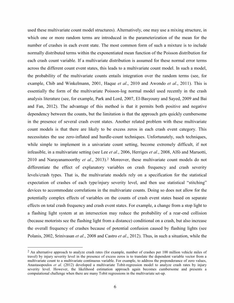
used these multivariate count model structures). Alternatively, one may use a mixing structure, in

which one or more random terms are introduced in the parameterization of the mean for the

number of crashes in each event state. The most common form of such a mixture is to include

normally distributed terms within the exponentiated mean function of the Poisson distribution for

each crash count variable. If a multivariate distribution is assumed for these normal error terms

across the different count event states, this leads to a multivariate count model. In such a model,

the probability of the multivariate counts entails integration over the random terms (see, for

example, Chib and Winkelmann, 2001, Haque et al., 2010 and Awondo et al., 2011). This is

essentially the form of the multivariate Poisson-log normal model used recently in the crash

analysis literature (see, for example, Park and Lord, 2007, El-Basyouny and Sayed, 2009 and Bai

and Fan, 2012). The advantage of this method is that it permits both positive and negative

dependency between the counts, but the limitation is that the approach gets quickly cumbersome

in the presence of several crash event states. Another related problem with these multivariate

count models is that there are likely to be excess zeros in each crash event category. This

necessitates the use zero-inflated and hurdle-count techniques. Unfortunately, such techniques,

while simple to implement in a univariate count setting, become extremely difficult, if not

infeasible, in a multivariate setting (see Lee et al., 2006, Herriges et al., 2008, Alfò and Maruotti,

2010 and Narayanamoorthy et al., 2013).2 Moreover, these multivariate count models do not

differentiate the effect of explanatory variables on crash frequency and crash severity

levels/crash types. That is, the multivariate models rely on a specification for the statistical

expectation of crashes of each type/injury severity level, and then use statistical “stitching”

devices to accommodate correlations in the multivariate counts. Doing so does not allow for the

potentially complex effects of variables on the counts of crash event states based on separate

effects on total crash frequency and crash event states. For example, a change from a stop light to

a flashing light system at an intersection may reduce the probability of a rear-end collision

(because motorists see the flashing light from a distance) conditional on a crash, but also increase

the overall frequency of crashes because of potential confusion caused by flashing lights (see

Polanis, 2002, Srinivasan et al., 2008 and Castro et al., 2012). Thus, in such a situation, while the

2 An alternative approach to analyze crash rates (for example, number of crashes per 100 million vehicle miles of travel) by injury severity level in the presence of excess zeros is to translate the dependent variable vector from a multivariate count to a multivariate continuous variable. For example, to address the preponderance of zero values, Anastasopoulos et al. (2012) developed a multivariate Tobit-regression model to analyze crash rates by injury severity level. However, the likelihood estimation approach again becomes cumbersome and presents a computational challenge when there are many Tobit regressions in the multivariate set-up.

7

count of non-rear-end collisions will increase because of a change from a stop sign to a flashing

light control, the count of rear-end collisions may increase or decrease, depending on whether the

overall count of crashes caused by general confusion overcomes or not the decrease in rear-end

collisions given a crash. More importantly, in this specific example, the net result on rear-end

collisions will vary across intersections based on other intersection characteristics (because count

models are non-linear models), and the only way to even try to mimic these complex effects in a

multivariate model would be to allow the covariance matrix to vary by intersection

characteristics. This is a tall order for a multivariate model system, and all extant multivariate

models assume a fixed covariance structure across the event count states across intersections,

which, in general, will not reflect the true impact of variables on crashes by event states.

2.1.2. Joint count and discrete choice and models

A second approach uses a strictly hierarchical combination of a count model to analyze total

crashes and a discrete choice model that allocates the total count to different injury severity

levels/crash types (see, for example, Kim et al., 2007, Huang et al., 2008 and Yu and Abdel-Aty,

2013). Also, the many studies in the literature that focus solely on total crashes or solely on

injury severity/crash type conditioned on a crash implicitly assume such a strictly hierarchical

mechanism for predicting crashes by injury severity level/crash type. In this hierarchical setting,

the probability of the observed counts in each injury severity level/crash type, given the total

count, takes a multinomial distribution form (see Terza and Wilson, 1990). This structure, while

easy to estimate and implement, is not very realistic for crash analysis. Thus, for example,

reconsider the case of a stop-sign controlled and a signal controlled intersection. Assume for now

that the difference between these two types of controls gets manifested in the crash type model

conditioned on a crash (because of say fewer rear-end collisions in the case of a signal-controlled

intersection). But say the difference between these two control types does not get included in the

total crash model because of statistical insignificance (after all, rear-end collisions are but a small

fraction of total crashes, because of which the difference in total crashes between stop-sign and

signal controlled intersections in the sample may not be adequate to tease out a statistically

significant effect of different controls in the total crash model).3 The necessary implication then

is that stop sign controlled intersections have fewer rear-end collisions relative to signal-

3 Such occurrences will be especially common place as the number of disaggregate event states (crash severity level and crash types) increases, since the number of crashes in each event state will be but a small fraction of total crashes.

8

controlled intersections, but a higher number of non-rear-end collisions (because the total

number of crashes is not affected by control type). This may not reflect ground reality. An

alternate and more appealing structure is one that explicitly links the event state discrete choice

model with the total crash count model. In this structure, one may use the expected value of the

highest crash type/injury severity risk propensity at an intersection from the event state

multinomial model as an explanatory variable in the conditional expectation for the total crash

count at the intersection (see Mannering and Hamed, 1990, Hausman et al., 1995, and

Rouwendal and Boter, 2009 for such a link between a choice model and a count model). This

explanatory variable may be viewed as a measure of the expected overall crash propensity at the

intersection. But a problem with this structure is that it fails to recognize the effects of

unobserved factors in the event state crash propensities on the total crash count (because only the

expected value enters the count model intensity, with no mapping of the event type propensity

errors into the count intensity). On the other hand, the factors in the unobserved portions of event

state crash propensities must also influence the total crash count intensity just as the observed

factors in the event state crash propensities do. This is essential to recognize the full econometric

jointness between the event state (given a crash) and the total crash count. In the case when a

generalized extreme value (GEV) model is used for the event state (as has been done in the past),

the maximum over the crash propensities is also GEV distributed, but including the resulting

error term in the count intensity leads to distributional mismatch issues. As indicated by Burda et

al. (2012), while the situation may be resolved by using Bayesian augmentation procedures,

these tend to be difficult to implement, particularly when random variations across observation

units (intersections in our case) in the effects of are also present in the event choice model.

2.2. The Current Study

In the current study, we use the second approach discussed above, while also accommodating the

full jointness in the total crash count and crash event state (crash type and injury severity level)

components of the model system. In doing so, we use a multinomial probit (MNP) model for the

crash event state discrete model (conditional on a crash), rather than the traditional multinomial

logit (MNL) or nested logit (NL) kernel used in earlier studies (as indicated by Lord and

Mannering, 2010, no study in the safety literature on injury severity or crash type has used an

MNP model, leave alone combining such a model with a total crash count model). The use of the

MNP kernel allows a more flexible covariance structure for the event states relative to traditional

9

GEV kernels. In our modeling framework, the MNP model also facilitates the linkage between

the crash event state and the total crash count components of the joint model system. In addition,

the model system allows random variations (or unobserved heterogeneity) in the sensitivity to

exogenous factors in both the crash event state (crash type/injury severity) model as well as the

total crash count components. The approach is based on the joint discrete and count model

proposed by Bhat et al. (2014), which uses a latent variable-based generalized ordered response

model representation for count data models (see Castro et al., 2012 to gainfully and efficiently

introduce the linkage from the crash type/injury severity model to the crash frequency model.

The formulation also allows handling excess of zeros in a straightforward manner (or excess

counts of any value), which is a common characteristic of crash counts (see Lord, 2006). The

resulting joint model is estimated using Bhat's (2011) frequentist MACML (for maximum

composite marginal likelihood) approach.

The approach is applied in a demonstration exercise to examine the number of motor

vehicle crashes at rural intersections in Central Texas by combinations of four crash types and

three injury severity levels. The data for the analysis is drawn from the Texas Department of

Transportation crash incident files. Explanatory variables considered in the analysis include

intersection attributes and major road characteristics.4

4 The major and minor roads of the intersection are defined as a function of the entering traffic flow. The database collected by the Texas Department of Transportation only includes characteristics of the major road; characteristics of the minor road(s) are not available.

11

CHAPTER 3: MODELING FRAMEWORK

3.1. Model Formulation

Let q ( Qq ,...,2,1 ) be an index to represent intersections and let i ( Ii ,...,2,1 ) be an index to

represent crash event states (i.e., combinations of crash types and injury severity levels). In the

empirical demonstration exercise in this thesis, there are four crash types (single vehicle crash,

angle crash with another vehicle, rear-end crash with another vehicle, and other crash types) and

three injury severity levels (no injury, possible injury, and confirmed injury ). The precise

definitions of the crash types and injury severity levels are provided later in Section 4.1. Thus,

there are 12 possible crash event states ( 12I ). Let k ),...,2,1,0( k be the index to represent

total crash frequency and let qn be the total number of crashes at intersection q over a certain

period of interest ( qn takes a specific value in the domain of k). Each count unit contribution to

the total count qn of crashes at intersection q corresponds to a crash instance in which one of the

I event states is manifested. Let t be an index for crash instance, so that t takes the values from

1 to qn for intersection q. As a result, the crash event discrete model takes the form of a panel

discrete choice model, with qn crash observations from intersection q. The resulting data allows

the estimation of intersection-specific unobserved factors that influence the intrinsic propensity

risk of each crash event state as well as the effects of other exogenous variables.

The next section (Section 3.1.1) presents the formulation for the crash event state model,

while the subsequent section (Section 3.1.2) develops the basic latent variable formulation for

the total crash frequency model. Section 3.1.3 presents the linkage specification between the

event state and the total count models. In the rest of this thesis, we will also use the following

key notations: ),( ΣbRMVN for the multivariate normal distribution of R dimensions with mean

vector b and covariance matrix Σ , RIDEN for an identity matrix of dimension R, R1 for a

column vector of ones of dimension R, R0 for a column vector of zeros of dimension R, and RR1

for a matrix of ones of dimension R×R.

12

3.1.1 Crash event state model

Let the propensity of observing crash event state i at crash instance t at intersection q be qtiS , and

write this propensity as a function of a (D×1) crash-level exogenous variable vector qix ( qix

includes a constant for all event states except one) as follows:

),(~~

,~

;~ ΩDDqqqqtiqiqqti MVNS 0ββbβxβ , (1)

where qβ is an intersection-specific (D×1)-column vector of corresponding coefficients. qβ is

assumed to be a realization from a multivariate normal density function with mean vector b and

covariance matrix Ω (this specification allows intersection-specific variation in the effects of

exogenous variables due to unobserved intersection/road attributes). qti~ is assumed to be an

independently and identically distributed (across crash instances and across intersections) error

term, but having a general covariance structure across crash event states at each crash instance.

Thus, consider the )1( I -vector ),,,,( 321 qtIqtqtqtqt εεεε ~~~~ε~ and assume that

),( ΘIIqt MVN 0~ε~ .

We now set out some additional notation. Define )( qtIqt2qt1qt S,...,S,SS (I×1 vector),

),...,,( 21

qqnqqq SSSS ( Inq 1 vector), ),...,,( 21 qtIqtqtqt εεε ~~~ε~ (I×1 vector),

),...,,( 21

qqnqqq ε~ε~ε~ε~ ( Inq 1 vector), and ),...,,( 21 qIqqq xxxx (I×D matrix). Then, we can

write:

qqqqqnqnq qqεVε~β

~bS x1x1 , (2)

where bV qnq qx1 and qεβε ~

~ qqnq q

x1 .

Next, let the crash event type observed at the tth

crash instance at intersection q be qtc

( Icqt ,...,2,1 ). Define qC as a ][)]1([ InIn qq block diagonal matrix, with each block

diagonal having )1( I rows and I columns corresponding to the tth

crash instance at intersection

q. This II )1( matrix for intersection q and crash instance t corresponds to an )1( I identity

matrix with an extra column of 1 values added as the th

qtc column. In the propensity

13

differential form (where the propensity differentials are taken with respect to the observed crash

event state qtc at each crash instance), we may write Equation (2) as:

qqqqqq

*

q εVSs CCC . (3)

Then, define qqnnq qqΩxx1Ω

~ ( InIn qq matrix) and ΘIDENΘ

qn

~

( InIn qq matrix). Let qqq VH C and qqqq CΘΩCA )(~~

. Finally, we obtain the result

below:

),(~ 1( qq)In

*

q qMVN AHs . (4)

The parameters to be estimated include the b vector, and the elements of the covariance

matrices Ω and Θ .5 The likelihood contribution of intersection q is the ))1(( Inq -

dimensional integral below:

111

)1(, )()(),()()0(),,(

qqqq qqIn

*

qstateeventcrashq PL AAA ωAωωΘΩ Hsb , (5)

where qAω is the diagonal matrix of standard deviations of qA .

The above likelihood function has a high dimensionality of integration, especially when

the total number of crashes qn and/or the number of crash event states I is high. To resolve this,

we use the MACML approach proposed by Bhat (2011), which involves the evaluation of only

univariate and bivariate cumulative normal distribution evaluations. However, note that the

5 Due to identification considerations (see Bhat et al., 2014), and if a very general covariance matrix is adopted, we

can only estimate a subset of the elements of Θ . While many normalizations may be used, we consider the

covariance matrix of the difference of the error terms qtiε~ with respect to the first error term

1~

qtε . That is, we

consider the )1()1( II covariance matrix 1Θ of

1qtε , where ),...,,( 131211 qtIqtqtqt εεεε and

1. i),~~( 11 qtqtiqti εεε The top diagonal matrix of 1Θ is constrained to one as a scale identification. In the estimation

process, Θ is effectively constructed from 1Θ by adding a top row of zeros and a first column of zeros. Of course,

one can place structure directly on Θ to obtain identification without estimating a general covariance matrix. Doing

so is particularly appealing when the number of alternatives is large, such as in our empirical context where I = 12. Thus, in our empirical context, we tested several error component structures starting from a covariance matrix corresponding to an error component specific to each crash type and each injury severity level. This specification accommodates unobserved crash-specific characteristics that affect each injury severity level across all types of crashes (for example, a crash-instance specific slippery pavement condition that increases the propensity of severe injuries of all crash types) and that affect each crash type across all injury severity levels (such as a temporary construction condition that increases the propensity of angled crashes of all injury severity levels). Note that one can use a similar (and efficient) error components structure at the intersection level for the random coefficients.

14

parameters from this model will also appear in the crash frequency model, and hence we discuss

the overall estimation procedure for the joint model in Section 3.2.

3.1.2 Crash frequency model

The crash frequency model is based on a Generalized Ordered Response Probit (GORP)

representation for count models formulated by Castro et al. (2012), who show that any count

model may be reformulated as a special case of a GORP model in which a single latent

continuous variable is partitioned into mutually exclusive intervals. This representation

generalizes traditional count models, can exactly reproduce any traditional count data model, and

allows handling excess zeros with ease.

Define the latent crash propensity for intersection q as *

qy and consider the following

structure:

qqqy wθq

*, kyq if qkqkq y

*

, 1 , with kqkqk f )z( , (6)

where qw is an (L×1)-column vector of exogenous attributes (excluding a constant), qθ is a

corresponding (L×1)-column vector of intersection-specific variable effects, and q is a random

error term assumed to be identically and independently standard normal distributed across

intersections. qθ is a realization from a multivariate normal density function with mean vector θ

and covariance matrix Ξ , such that qq θ~

θθ and ),( ΞLLq MVN 0~θ~

is independent of q ( qθ~

is an intersection-specific coefficient vector introduced to account for unobserved heterogeneity

in the latent crash propensity). The latent crash propensity *

qy is mapped to the observed ordinal

variable qy by the thresholds qk , which satisfy the ordering conditions ( 1,q ;<

...)210 qqq in the usual ordered-response fashion, )( qkf z is a non-linear function of a

vector of intersection-specific variables qz ( qz includes a constant), and k is a scalar similar to

the thresholds in a standard ordered-response model 0;( 01 for identification, and

...)0 21 . Write ,!

z

k

l

l

q

qkl

ef q

0

1)(

so that the thresholds in Equation (6) take

the following form:

15

k

k

l

l

q

qkl

e q

0

1

!, with qeq

γz , and *Kk if *Kk ,

(7)

where 1 is the inverse function of the univariate cumulative standard normal, γ is a

coefficient vector to be estimated, and *K is an appropriate count level that may be determined

based on the empirical context under consideration and empirical testing. The presence of the k

term provides flexibility to accommodate high or low probability masses for specific count

outcomes without the need for using hurdle or zero-inflated mechanisms. Also note that qw and

qz can have common elements.

The proposed crash frequency model can be motivated from an intuitive standpoint. In

our empirical context, the latent long-term crash propensity *

qy of intersection q may be

impacted by intersection-specific variables that would get manifested in the qw vector. On the

other hand, there may be some specific intersection characteristics (embedded in qz ) that may

increase/decrease the likelihood of crash occurrence at any given instant of time for a given long-

term crash propensity *

qy . The presence of intersection characteristics in qz allows intersections

with the same latent crash propensity to have different observed crash frequency outcomes. The

reader is referred to Castro et al. (2012) for more details of the intuitive interpretation of the

GORP recasting of count models.

3.1.3. Joint crash frequency - crash event state model

At each crash instance, a measure of the overall crash propensity may be obtained as the

maximum of the value across the crash event state (type/injury severity level) risk propensities.

This variable can then be included as an explanatory variable in the crash frequency model along

with other variables. To develop this link, consider the expression for the crash risk propensity of

crash event state i at crash instance t ),...,2,1( qnt at intersection q in Equation (1). Because the

exogenous variables (and the corresponding coefficients) are specific to each intersection, and

the error terms qti~ are assumed to be independently and identically distributed (across crash

instances and across intersections), we may write the crash risk propensity of crash event state i

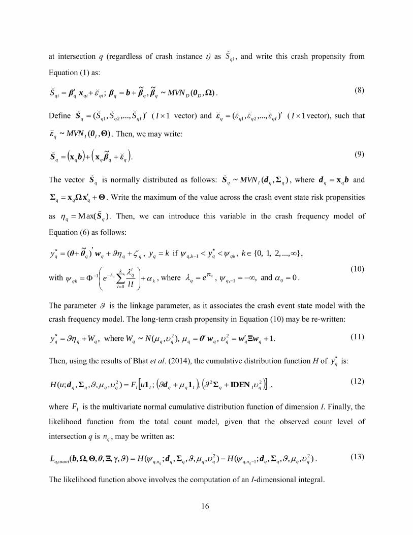
16

at intersection q (regardless of crash instance t) as qiS

, and write this crash propensity from

Equation (1) as:

),(,; ΩDDqqqqiqiqqi MVNS 0~β~

β~

bβxβ

. (8)

Define ),...,,( 21 qIqqq SSS

S ( 1I vector) and ),...,,( 21

qIqqq εεε

ε ( 1I vector), such that

),( ΘIIq MVN 0~ε

. Then, we may write:

qqqqq εβ~

bS

xx . (9)

The vector qS

is normally distributed as follows: ),( qqIq MVN Σd~S

, where bd qq x and

ΘxΩxΣ qqq . Write the maximum of the value across the crash event state risk propensities

as )(Max qq S

. Then, we can introduce this variable in the crash frequency model of

Equation (6) as follows:

qqqqqy wθ~

θ* )( , kyq if qkqkq y

*

, 1 , }..., ,2,1,0{ k ,

with k

k

l

l

q

qkl

e q

0

1

!, where qeq

γz , 0and, 01 ,q .

(10)

The parameter is the linkage parameter, as it associates the crash event state model with the

crash frequency model. The long-term crash propensity in Equation (10) may be re-written:

.1,),,(where, 22 qqqqqqqqqqq NWWy wwwθ~*

Ξ (11)

Then, using the results of Bhat et al. (2014), the cumulative distribution function H of *

qy is:

222 ,;),,,,;( qIqIqqIIqqqq uFuH IDENΣ11Σ dd , (12)

where IF is the multivariate normal cumulative distribution function of dimension I. Finally, the

likelihood function from the total count model, given that the observed count level of

intersection q is qn , may be written as:

),,,,;(),,,,;(),γ,,,,,( 2

1,

2

, qqqqnqqqqqnqcountq, qqHHL ΣΣΞΘΩ ddθb . (13)

The likelihood function above involves the computation of an I-dimensional integral.

17

3.2. Model Estimation

The overall likelihood function for the joint crash frequency-crash event state model may be

obtained from Equations (5) and (13) as follows:

),γ,,,,,(),,(),γ,,,,,( ,, ΞΘΩΘΩΞΘΩ θbbθb countqstateeventcrashqq LLL . (14)

To address the issue of the high dimensionality of integration in stateeventcrashqL , (of dimension

))1( Inq in the above function, we replace the log-likelihood from the event state model with

a composite marginal likelihood (CML), CML

stateeventcrashqL , . The CML approach, which belongs to

the more general class of composite likelihood function approaches (see Lindsay, 1988), may be

explained in a simple manner as follows. In the crash event state model, instead of developing

the likelihood of the entire sequence of repeated observations (crashes) from the same

intersection, consider developing a surrogate likelihood function that is the product of the

probability of easily computed marginal events. For instance, one may compound (multiply)

pairwise probabilities of outcome qtc at intersection q at crash instance t and outcome tqc at

intersection q at crash instance t' , of outcome qtc at intersection q at crash instance t and

outcome tqc at intersection q at crash instance 't , and so forth. The CML estimator (in this

instance, the pairwise CML estimator) is then the one that maximizes the compounded

probability of all pairwise events. The properties of the CML estimator may be derived using the

theory of estimating equations (see Cox and Reid, 2004, Yi et al., 2011). Specifically, under

usual regularity assumptions (Molenberghs and Verbeke, 2005; Xu and Reid, 2011), the CML

estimator is consistent and asymptotically normal distributed, and its covariance matrix is given

by the inverse of (Godambe, 1960) sandwich information matrix (see Zhao and Joe, 2005).

Letting the index of the crash outcome at crash instance t at intersections q to be qtM , the

CML function for the crash event state model for intersection q may be written as:

1

1 1

1

1 1

1

1 1

,

)0( )0and 0(

),(

q qq q

q q

n

t

n

tt

*

tqt

n

t

n

tt

*

tq

*

qt

n

t

n

tt

tqtqqtqt

CML

stateeventcrashq

ProbProb

cMcMProbL

sss

(15)

18

where

*

tq

*

qt

*

tqt sss ,

. Then,

111

12 )()();()()0(

tqttqttqt tqtI

*

tqtP AAA ωAωω

tqt)( Hs (16)

where ),( qt'qttqt HHH

, qtH is the sub-vector of qH that includes elements corresponding to

the tth

crash instance, tqt A is the 2×2-sub-matrix of qA that includes elements corresponding to

the tth

and tht crash instances, and ttq Aω

is the diagonal matrix of the standard deviations of

tqt A . Finally, the function to be maximized to obtain the parameters is:

),,,,,,(),,(),,,,,,( ,, γθbbγθb ΞΘΩΘΩΞΘΩ countq

CML

eventstatecrashq

CML

q LLL (17)

The CML

stateeventcrashqL , component in the equation above entails the evaluation of a multivariate

normal cumulative distribution (MVNCD) function of dimension equal to 2)1( I , while the

countqL , component involves the evaluation of a MVNCD function of dimension .I But these may

be evaluated using the approximation part of the maximum approximate composite marginal

likelihood (MACML) approach of Bhat (2011), leading to solely bivariate and univariate

cumulative normal function evaluations.

One additional issue still needs to be dealt with. This concerns the positive definiteness of

several matrices in Equation (17). Specifically, for the estimation to work, we need to ensure the

positive definiteness of the following matrices: , , ΘΩ and Ξ . This can be guaranteed in a

straightforward fashion using a Cholesky decomposition approach (by parameterizing the

function in Equation (17) in terms of the Cholesky-decomposed parameters).

3.3. Model Fit Issues

3.3.1 Model selection

Procedures similar to those available with the maximum likelihood approach are also available

for model selection with the CML approach (see Varin and Vidoni, 2008). The statistical test for

a single parameter may be pursued using the usual t-statistic. When the statistical test involves

multiple parameters between two nested models, an appealing statistic, which is also similar to

the likelihood ratio test in ordinary maximum likelihood estimation, is the adjusted composite

likelihood ratio test (ADCLRT) statistic (see Pace et al., 2011 and Bhat, 2011 for details).

19

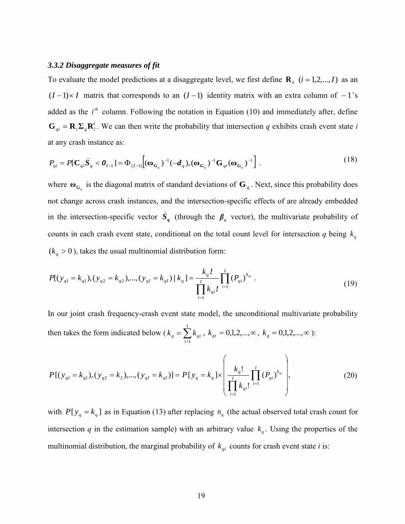
3.3.2 Disaggregate measures of fit

To evaluate the model predictions at a disaggregate level, we first define iR ),...,2,1( Ii as an

II )1( matrix that corresponds to an )1( I identity matrix with an extra column of 1 ’s

added as the thi column. Following the notation in Equation (10) and immediately after, define

iqiqi RΣRG . We can then write the probability that intersection q exhibits crash event state i

at any crash instance as:

111

)1(1 )()(),()(][

qqq qiqIIqqiqi PP GGG ωGωωC d0S

. (18)

where qGω is the diagonal matrix of standard deviations of qG . Next, since this probability does

not change across crash instances, and the intersection-specific effects of are already embedded

in the intersection-specific vector qS

(through the qβ vector), the multivariate probability of

counts in each crash event state, conditional on the total count level for intersection q being qk

0( qk ), takes the usual multinomial distribution form:

I

i

k

qiI

i

qi

q

qqIqIqqqqqiP

k

kkkykykyP

1

1

2211 )(])(),...,(),[(

!

!| .

(19)

In our joint crash frequency-crash event state model, the unconditional multivariate probability

then takes the form indicated below (

I

i

qiq kk1

, ,...,2,1,0qik , ,...,2,1,0qk ):

I

i

k

qiI

i

qi

q

qqqIqIqqqqiP

k

kkyPkykykyP

1

1

2211 )(

!

!][)](),...,(),[( , (20)

with ][ qq kyP as in Equation (13) after replacing qn (the actual observed total crash count for

intersection q in the estimation sample) with an arbitrary value qk . Using the properties of the

multinomial distribution, the marginal probability of qik counts for crash event state i is:

20

0

)1()()(

][][q

qiqqi

k

kk

qi

k

qi

qiqqi

q

qqqiqi PP!kk!k

!kkyPkyP (21)

In the above expression, the upper bound of the summation is qk , though the probability

values fade very rapidly beyond a qk value of 5. For the purposes of this thesis, we carry the

summation up to .20qk

Then, at the disaggregate level, we can estimate the probability of the observed

multivariate count category for each intersection using Equation (20), and compute an average

probability of correct prediction. Similarly, we also can estimate the probability of the observed

marginal count event state separately for each crash type/injury severity level using Equation

(21), and compute an average probability of correct prediction.

3.3.3 Aggregate measures of fit

At the aggregate level, we design a heuristic diagnostic check of model fit by computing the

predicted aggregate share of intersections in specific multivariate outcome states (because it

would be infeasible to provide this information for each possible multivariate outcome state). In

particular, we predict the aggregate share of intersections in each of 13 crash event combination

states. The first combination event state corresponds to zero crashes (which we will refer to as

the “no crashes” state). The other 12 combination states correspond to crash counts in each crash

type/injury severity state and no crashes in any other crash type/injury severity state. In addition

to these aggregate shares of multivariate outcomes, we also compute the aggregate shares of the

marginal outcomes of crash count values of 0, 1 and 2+ for each crash event state. To evaluate

the performance of the model proposed here, we compute the absolute percentage error (APE)

statistic for each combination state (as the difference between the predicted and observed values

for each count combination state as a percentage of the observed value), and then compute a

mean weighted APE value across the count values (of 0 1 and 2+) using the observed number for

each count value as the weight for that count value

21

CHAPTER 4: DATA

4.1. Sample Formation

The crash data used in the analysis is drawn from the Texas Department of Transportation

(TxDOT) Crash Records Information System (CRIS) for the year 2010. The CRIS compiles

police and driver reports of crashes into multiple text files, including complete crash, person, and

vehicle-related details for each crash.6 The crash files include information of crash type and

injury severity, along with crash time and location, and weather and lighting-related

characteristics. TxDOT overlays the crash location from the crash files to a Geographic

Information System (GIS)-based street network, identifies crash locations on the street network,

and extracts the characteristics of each crash, along with supplementary information on

intersection and road design, geometric variables, and traffic conditions.

For the current study, intersection and intersection-related crashes occurring in rural areas

of central Texas were extracted from the CRIS data base.7 Central Texas, as used in this thesis,

includes the districts of Austin and San Antonio.8 This area was selected to include two of the

most densely populated cities in Texas (Austin and San Antonio) and a tract of about 400 miles

of Interstate 35 (I-35) with associated frontage roads and intersections. The dependent variable of

our analysis is the count of all traffic crashes at rural intersections in the year 2010 by

combinations of crash type and injury severity level. Due to the difference in the nature and

characteristics of injury severity and crash type between crashes involving only motorized

vehicles and those also involving non-motorized vehicles (pedestrians and bicyclists) and/or

trains (see Bagdadi, 2013), only the pool of motor-vehicle crashes were considered in the current

analysis. Also, the records of independent variables with incomplete or inconsistent information

on crash and intersection design were removed from the sample. Our sample formation

procedure thus far includes only those intersections for which at least one crash occurred in

2010. This is because, for those intersections at which no crashes occurred that year, we do not

have readily available information on intersection attributes (because the intersection attributes

6 The Texas law enforcement agency officially maintains the records of those crashes reported by police and drivers that involve property damage of more than $1,000 and/or the injury or death of one or more individuals. Then, by construction, there is an under-reporting of the “no injury” category in the CRIS database, and so our analysis could be viewed as focused on the population of crashes that are biased toward higher injury severity.

7 TxDOT defines an intersection-related crash as those that occur within the curbline limits of intersections or on one of the approaches/exits to the intersection within 200 feet from the intersection center point.

22

are available only for those intersections that appear in the CRIS data base, and intersections at

which no crashes occurred in 2010 do not appear in the 2010 CRIS files). To alleviate this

selection problem and reduce the resulting bias, we identified intersections in which there was at

least one crash during 2009 (and, therefore, intersection design characteristics were available),

but that did not appear in the 2010 CRIS file. These intersections were then appended to our

sample, setting the number of crashes at these intersections to zero. Overall, our analysis may be

viewed as being focused on the relatively crash-prone rural intersections in central Texas.

The final estimation sample at the end of the sample formation process discussed above

includes 1348 rural intersections. The total number of crashes in the sample is 798,

corresponding to an average of 0.59 crashes per intersection and an average of 1.39 crashes per

intersection for those intersections with at least one crash. Figure 1 presents the distribution of

crashes across all intersections, showing that 57.5% of the intersections in the sample have zero

crashes (as obtained from the 2009 CRIS file with no corresponding entry from the 2010 CRIS

file) and 42.5% have at least one crash. This excess of zeros, commonly present in crash data, is

not a problem in our proposed framework because of the flexible specification of the thresholds

of the count data model (see Section 3.1.2). Figure 1 also shows that one intersection has an

exceptionally large number of crashes (19 crashes in one year).9 This observation, usually

considered an outlier, can also be modeled by our count data approach (see El-Basyouny and

Sayed, 2010 for an analysis of outliers in crash data).

8 TxDOT defines districts to oversee the construction and maintenance of state highways. The Texas districts definitions are available at http://www.txdot.gov/inside-txdot/district.html 9 This intersection is located at the exit of a hospital located between the cities of Buda and Kyle. Crashes at this intersection are mostly angle crashes with no injured occupants.

http://www.txdot.gov/inside-txdot/district.html

23

Figure 1. Crash frequency distribution across intersections

As discussed earlier, the multivariate dependent variable in our analysis is the number of

crashes by combinations of crash type and injury severity level. In the CRIS file, crash types are

coded in 42 distinct categories. Based on the frequency of each crash type in the final sample, we

aggregated the crash types into four categories:10 (1) single-vehicle (only one vehicle is involved

in the crash), (2) angle (two vehicles moving at an angle to one another just before the point of

impact)), (3) rear-end (the front of one moving vehicle crashes into the back of another moving

vehicle traveling in the same direction), and (4) other crash types (including head-on collisions,

sideswipe collisions and collisions with two vehicles backing; these crash types are aggregated

into one category because of the very few crashes within each of the crash types individually).

The injury severity level associated with a crash, as used in the current analysis, corresponds to

the most severely injured individual (could be a driver or a passenger) in the crash. Injury

severity is recorded in five ordinal categories: (1) no injury, (2) possible injury, (3) non-

10 Although the crash types used for the analysis may seem overly-aggregated, the 42 categories defined in the CRIS files were extremely fine (one could say almost overly fine to be able to discriminate based on the explanatory variables usually available for prediction of crashes). For example, angle crashes were categorized into 10 groups, based on the direction in which the vehicles were moving at the moment of the impact (turning, going straight, backing). Besides, the number of crashes in each of these 10 categories was fairly low, with the variation in the number of crashes in each category not being adequate for statistical inference and analysis.

24

incapacitating injury, (4) incapacitating injury, and (5) fatal injury. Because of the very low share

of crashes with incapacitating and fatal injuries (4.3% and 1.6%, respectively), we converted the

five-level ordinal categorization into a three-level scheme by combining the non-incapacitating,

incapacitating and fatal categories into a single level denoted “confirmed injury”. Based on the

four crash type categories and three injury severity levels, there is a total of 12 crash event states.

Table 1 shows the number of crashes by each of these categories, and the corresponding

percentages. The last column of the table reveals that angled crash types are the most prevalent,

with rear-end and other crash types also occurring quite often. Single vehicle crashes are the

fewest, though they also make up more than 10% of all crashes. The last row of the table

indicates that more than half of all crashes did not result in any injuries, while the remaining

crashes were about equally split between crashes with possible injury and crashes with

confirmed injuries. The most prevalent type of crash by type and injury severity level is an

angled crash with no injury (20.2% of total crashes). The table also shows differences in the

patterns of injury severity based on type of crash (see the columns entitled “Crashes as a

percentage of row total” in Table 1). Thus, angled crashes are less likely to lead to no injury, and

more likely to lead to confirmed injury, compared to other types of crashes. Single vehicle

crashes are the most likely to lead to no injury, while rear-end crashes are the least likely to lead

to confirmed injury.

The next section discusses additional sample characteristics on relevant exogenous

variables in the analysis.

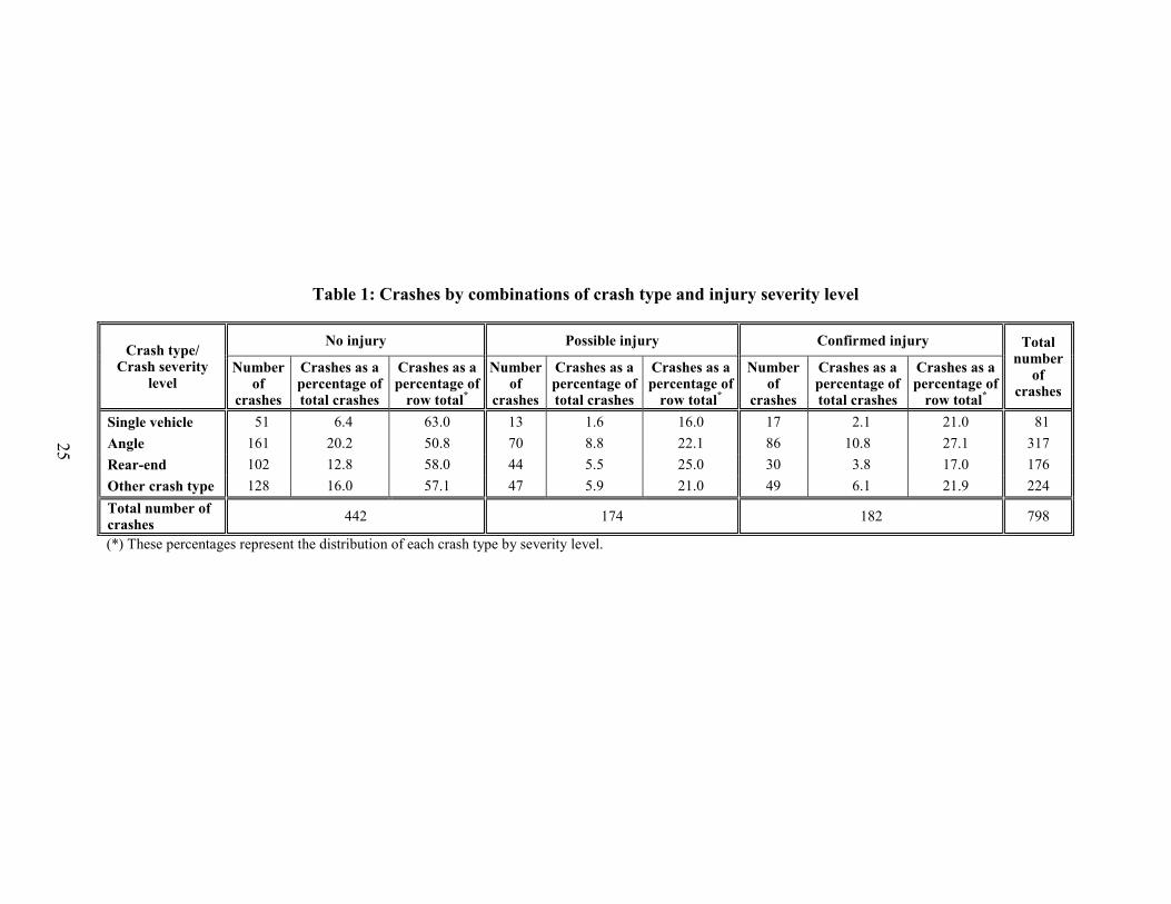
Table 1: Crashes by combinations of crash type and injury severity level

Crash type/ Crash severity

level

No injury Possible injury Confirmed injury Total number

of crashes

Number of

crashes

Crashes as a percentage of total crashes

Crashes as a percentage of

row total*

Number of

crashes



row total*

Number of

crashes



row total*

Single vehicle 51 6.4 63.0 13 1.6 16.0 17 2.1 21.0 81

Angle 161 20.2 50.8 70 8.8 22.1 86 10.8 27.1 317

Rear-end 102 12.8 58.0 44 5.5 25.0 30 3.8 17.0 176

Other crash type 128 16.0 57.1 47 5.9 21.0 49 6.1 21.9 224

Total number of crashes

442 174 182 798

(*) These percentages represent the distribution of each crash type by severity level.

25

26

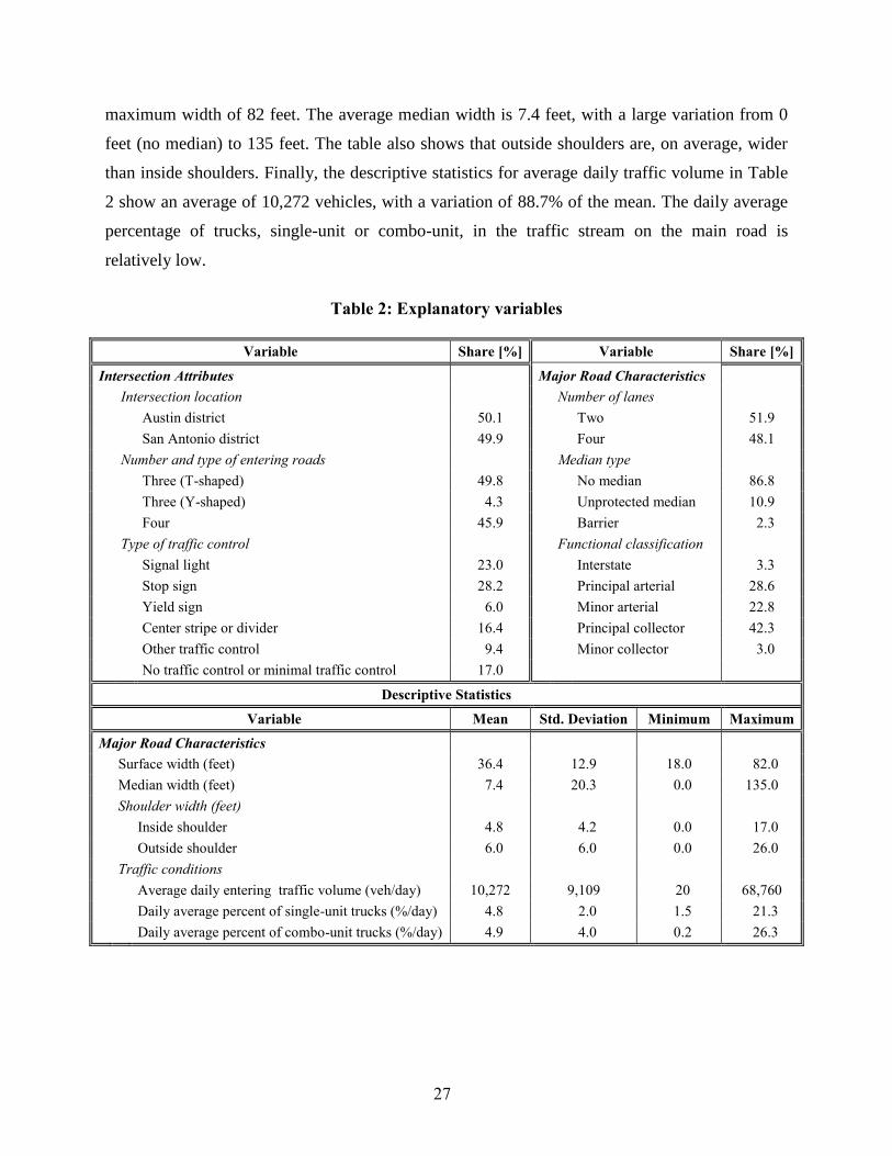
4.2. Sample Characteristics

Several types of exogenous variables were considered in the empirical analysis, including

intersection attributes and major road characteristics (the major road of an intersection is defined

as the entering road with the highest traffic volume). Table 2 presents the sample characteristics

of selected exogenous variables within each of these categories of variables.11

Intersection attributes include (1) intersection location variables, which are indicator

variables for the Austin and San Antonio districts to account for possible overall location-related

factors that are not able to be captured by other explanatory variables, (2) number and type of

entering roads, and (3) type of traffic control. Table 2 indicates that the number of entering roads

is three for more than half of the intersections, both in T-shape form as well as Y-shape form. In

addition, there are a sizeable number of intersections with four entering roads. The traffic control

type statistics indicate that more than half of the intersections are controlled by either a signal

light or a stop sign (i.e., a stop sign on one or more approaches, but no other form of control),

while yield sign controlled intersections (a yield sign on one or more approaches) are fairly

uncommon (only 6%). Intersections with a center stripe or divider represent 16.4% of the

estimation sample, and intersections with other traffic controls (such as flashing lights, marked

lanes or no passing zone signs) account for 9.4% of the sample. Finally, a considerable number

of intersections have no traffic control (an intersection is designated as having no control if it

does not have any of the previous control types).

The major road characteristics include number of lanes, median type, functional

classification,12 surface width (for both travel directions, not including shoulders or median

width), median width, inside and outside shoulder widths (the inside shoulder is to the left of the

direction of movement, while the outside shoulder is to the right of the direction of movement),

and traffic conditions. Table 2 shows that the number of approach lanes on the major road is

almost equally distributed among two and four lanes, and that more than 85% of the major roads

have no median. Regarding functional classification, most major roads are principal collectors,

representing 42.3% of the sample, followed by principal and minor arterials, with 28.6% and

22.8%, respectively. The average surface width is 36.4 feet, with a minimum of 18 feet and a

11 Some explanatory variables were not statistically significant in the final model specification; the sample characteristics of these variables are not presented in Table 2 to conserve on space. Among these variables were: roadway alignment (horizontal curvature or vertical grade), and lane type (two-lane, boulevard, expressway or highway). 12 Functional classification as defined by the FHWA can be found at: http://ntl.bts.gov/lib/23000/23100/23121/09RoadFunction.pdf

http://ntl.bts.gov/lib/23000/23100/23121/09RoadFunction.pdf

27

maximum width of 82 feet. The average median width is 7.4 feet, with a large variation from 0

feet (no median) to 135 feet. The table also shows that outside shoulders are, on average, wider

than inside shoulders. Finally, the descriptive statistics for average daily traffic volume in Table

2 show an average of 10,272 vehicles, with a variation of 88.7% of the mean. The daily average

percentage of trucks, single-unit or combo-unit, in the traffic stream on the main road is

relatively low.

Table 2: Explanatory variables

Variable Share [%] Variable Share [%]

Intersection Attributes Major Road Characteristics

Intersection location Number of lanes

Austin district 50.1

Two 51.9

San Antonio district 49.9

Four 48.1

Number and type of entering roads Median type

Three (T-shaped) 49.8

No median 86.8

Three (Y-shaped) 4.3

Unprotected median 10.9

Four 45.9

Barrier 2.3

Type of traffic control Functional classification

Signal light 23.0

Interstate 3.3

Stop sign 28.2

Principal arterial 28.6

Yield sign 6.0

Minor arterial 22.8

Center stripe or divider 16.4

Principal collector 42.3

Other traffic control 9.4

Minor collector 3.0

No traffic control or minimal traffic control 17.0

Descriptive Statistics

Variable Mean Std. Deviation Minimum Maximum

Major Road Characteristics

Surface width (feet) 36.4 12.9 18.0 82.0

Median width (feet) 7.4 20.3 0.0 135.0

Shoulder width (feet)

Inside shoulder 4.8 4.2 0.0 17.0

Outside shoulder 6.0 6.0 0.0 26.0

Traffic conditions

Average daily entering traffic volume (veh/day) 10,272 9,109 20 68,760

Daily average percent of single-unit trucks (%/day) 4.8 2.0 1.5 21.3

Daily average percent of combo-unit trucks (%/day) 4.9 4.0 0.2 26.3

29

CHAPTER 5: ESTIMATION RESULTS

5.1. Variable Specification

The selection of variables included in the final model specification was based on previous

research, intuitiveness, and parsimony considerations. For categorical exogenous variables, if a

certain level of the variable did not have sufficient observations, it was combined with another

appropriate level; and if two levels had similar effects, they were combined into one level. For

continuous variables, we tested alternative linear and non-linear functional forms, including

dummy variables for different ranges. The intersection attributes and major road characteristics

were considered both in the crash frequency model specification (threshold and long-term

propensity) and in the crash event state model specification.

The final estimation results are presented in Table 3 (for the crash frequency model) and

Table 4 (for the crash event state model). In some cases, we have retained variables that are not

statistically significant at a 0.05 significance level because of their intuitive effects and to inform

future research efforts in the field.

Table 3: Joint model estimation results - Crash frequency model

Variables

Latent Propensity Coefficients

Threshold Coefficients

Estimate t-stat Estimate t-stat

Constants

Constant in vector -2.5277 -2.168

Threshold specific constants

α1 0.9367 2.017

α2 0.7858 1.296

Intersection attributes

Number and type of entering roads (three (T-shaped))

Three (Y-shaped) 0.6668 1.812

Four -0.8488 -1.787

Type of traffic control (signal light)

Stop sign -1.2134 -2.636

Yield sign -1.2064 -2.630

Center stripe or divider -1.0683 -3.090

Other traffic control -0.5575 -1.838

No traffic control or minimal traffic control -1.8023 -3.544

Major road characteristics

Traffic conditions

Average daily entering traffic volume (veh/day/1,000)

-0.0152 -1.762

Linkage parameter 1.8414 2.803

30

Table 4: Joint model estimation results - Crash event state model

Variables Estimate t-stat

Constants

Single vehicle/Possible injury -0.7479 -1.555

st. deviation 0.6102 1.264

Single vehicle/Confirmed injury -0.5819 -1.699


Angle/No injury -0.4465 -3.343

Angle/Possible injury -0.5152 -6.279

Angle/Confirmed injury 0.2766 1.072

Rear-end/No injury 0.0149 0.120


Rear-end/Possible injury 0.0845 1.071

Rear-end/Confirmed injury -0.6346 -1.405


Other crash type/No injury 0.3791 4.896


Other crash type/Possible injury -0.4607 -3.673

Other crash type/Confirmed injury 0.0132 0.234


Intersection location

San Antonio district (Austin district)

Angle/No injury -0.3117 -4.760

Type of traffic control (signal light)

Stop sign

Angle/No injury 1.1127 14.648

Angle/Possible injury 1.1096 18.004


Yield sign



Number of lanes (two)

Four

Angle/Possible injury 0.5685 8.000


Traffic conditions

Logarithm of average daily entering traffic volume (ln(veh/day/1,000))

Other crash type/Possible injury 0.1869 3.647

Surface width (feet)


Angle/Confirmed injury -0.0260 -2.731


Inside shoulder

Single vehicle/Confirmed injury -0.0413 -1.614

Outside shoulder

Single vehicle/Possible injury -0.0333 -1.618

Rear-end/Possible injury -0.0241 -2.798

31

5.2. Estimation Results Analysis

5.2.1 Crash frequency model

The first main numeric column of Table 3 provides the coefficients associated with the latent

propensity, while the second main numeric column presents the threshold coefficients. In these

tables, for categorical variables, the base category is presented in parenthesis. For example, for

“Number and type of entering roads”, the base category is “three (T-shaped)”. Also, a positive

sign for a latent propensity coefficient indicates that an increase in the corresponding variable

results in an increased crash frequency propensity, while a negative sign indicates the reverse.

For the threshold variables, a positive coefficient shifts the threshold toward the left of the

propensity scale, which has the effect of reducing the probability of the zero-crash outcome

(increasing the overall probability of the non-zero outcome). A negative coefficient, on the other

hand, shifts the threshold toward the right of the propensity scale, which has the effect of

increasing the probability of the zero-crash outcome (decreasing the overall probability of the

non-zero outcome crashes).

The first row panel in Table 3 presents the constant in the vector, as well as the

threshold-specific constants k( values). These constants do not have any substantive

interpretations, though the threshold specific constants )( k provide flexibility in the count

model to accommodate high or low probability masses for specific outcomes. As indicated in

Section 3.1.2, identification is achieved by specifying 00 and KkKk . In the

present specification, we initially set K = 19 (which is the maximum value of the total number of

crashes in the sample) and progressively reduced K based on statistical significance

considerations and general data fit. The final specification in Table 3 is based on setting K = 2.

The next row panel of Table 3 provides the effects of intersection attributes. The results

show that Y-shaped intersections have a higher crash risk propensity than T-shaped intersections.

It is possible that drivers do not perceive Y-shaped intersections as a stop-and-go location

because of the skew angle of the lanes and, therefore, fail to give the right-of-way or to slow

down when reaching the intersection. The results also show that a given crash risk propensity is

more likely to get translated into a non-zero crash outcome at intersections with four entering

roads relative to intersections with three T-shaped entering roads, as indicated by the negative

sign in the threshold coefficient. This result has been found in safety literature before (Qin et al.,

2010, Castro et al., 2012) and can be attributed to the fact that three-legged intersections have

32

fewer conflicting points and may provide more of an “out” to drivers to avoid crashes once a

potential crash situation starts to develop. The results pertaining to the type of traffic control

show that intersections with a signal light have a higher crash risk propensity than other forms of

control. In particular, intersections with no traffic control or minimal traffic control have the

lowest crash risk propensity (see Bullough et al., 2013 for the same result). A plausible

explanation is that drivers do not expect to face signal lights in rural areas and do not react in

time to possible intersection-related hazards. Another possibility is that the type of traffic control

is highly correlated with traffic volume, which may be the underlying cause of high number of

crash counts (even after incorporating traffic volume as an exogenous variable). This

endogeneity problem is out of the scope of this study, but readers are referred to Bhat et al.

(2014) for details on count data models with endogenous covariates.

Among major road characteristics, the only variable that significantly contributes toward

explaining crash frequency is the average daily entering traffic volume. The negative coefficient

implies that intersections with high traffic volume in the major road have a reduced crash risk

propensity. This finding may be due to reduced speeds because of traffic congestion, which

allows the drivers more time to react and avoid collisions. Since the traffic volume is not the total

entering volume for the intersection, but the entering volume of the major road only.

Consequently, it is possible that drivers in the minor road are more cautious when approaching

the intersection and that helps to reduce crash frequency when facing an intersecting road with

high traffic volume (see Castro et al., 2012).

The parameter that links the crash event state model with the crash frequency model in

our final model specification is statistically significant, supporting the hypothesis that the

frequency of crashes and the crash even state outcomes of these crashes are interrelated. That is,

the total count of crashes is endogenous to the combinations of crash type and injury severity

levels, and variables that affect the event state also impact the total count of crashes through the

linkage parameter.

5.2.2 Crash event state model

Table 4 presents the results of the crash event state model. Although we extensively tried to

accommodate a flexible correlation matrix for the crash event states, no coefficients resulted

significant. Therefore, the model presented in this table was estimated assuming that the crash

event states and identically and independently (IID) distributed. The first row panel of Table 4

33

presents the alternate specific constants, with the base alternative being the single vehicle/no

injury crash event state. These constants do not have any substantive interpretation because of

the presence of continuous explanatory variables. However, some of these constants have a

significant standard deviation, indicating intersection-specific heterogeneity in the crash event

state outcomes.

Intersection attributes are significant determinants of crash event state occurrence.

Compared with intersections located in Austin district, intersection in San Antonio district are

less likely to result in angle crashes in which no one is injured. This indicator variable is

capturing the mean effect of all unobserved factors not considered in our analysis (such as traffic

congestion effects and speed limit) and does not have a substantive interpretation. The type of

traffic control is also a significant determinant of crash event state. Table 4 shows that, compared

to intersections controlled by signal lights, intersections controlled by stop signs tend to present a

higher likelihood of angle crashes, for the three injury severity levels. Also, there is a trend in

these coefficients, such that the outcome of angles crashes at stop-controlled intersections is

more likely to be no injury and less likely to be confirmed injury. The increased likelihood of

angle crashes at intersections controlled by stop signs could be because some drivers do not

respect the right-of-way and collide against vehicles traveling in the other road (Retting et al.,

2003). In addition, stop-sign controlled intersections require that drivers establish the adequate

gap in the conflicting traffic to cross the intersection; if this gap is not established correctly,

angle crashes are more likely to occur. Similar to stop-controlled intersections, intersections

controlled with yield signs present more angle/no injury crashes than signal controlled

intersections, maybe for the same reasons discussed before (although the coefficient magnitude

and its significance are considerably lower).

In the category of major road characteristics, major roads with four lanes increase the

likelihood of severe (possible injury and confirmed injury) angle crashes, compared to major

roads with two lanes. It is possible that drivers in minor roads misestimate the crossing distance

of wider roads (four-lane roads) and, therefore, do not allocate enough time to cross the

intersection and collide against vehicles traveling in the major road. The logarithm of the average

daily entering traffic volume impacts the occurrence of the crash event state other crash

type/possible injury. This finding could be due to an increase in exposure for other crash types,

such as head-on and sideswipe crashes (see Aguero-Valverde and Jovanis, 2009 and Park and

Lord, 2007 for a similar finding). Finally, surface and shoulder width tend to reduce crash

34

severity for different crash types (for similar results, see Mitra and Washington, 2007, Ma et al.,

2008, and Pei et al., 2011). The table shows that wider major roads present more angle crashes in

which no passenger is injured (as found by Ye et al., 2009) and less angle crashes with possible

injuries. It is possible that wider road surfaces allow drivers to circumvent, at some extent, other

vehicles; then, intersection design with wide major roads can improve angle crash safety.

Similarly, major roads with wider shoulders, either interior or exterior, are less prone to present

crashes resulting in possible or confirmed injury, for different crash types. Moreover, because of

the negative signs of the coefficients associated with surface and shoulder width, wider major

roads will result in a reduced crash frequency, as discussed in Section 5.4.

Overall, these results validate the approach undertaken in this study, showing that

intersection-specific variables have differential impacts on crash types and severity levels.

5.3. Measures of Fit

The composite log-likelihood (CLL) measure of the joint crash frequency-crash event state

model (the joint model) is -3,645.8 with 41 parameters. The corresponding figure for the model

system that unlinks the total crash frequency model and the crash event state model (the

independent model) is -3,659.1 with 40 parameters. As discussed in Section 3.3, these CLL

measures can be compared by computing the ADCLRT statistic, which returns a value of 18.4,

which is larger than the table chi-squared value with one degree of freedom at any reasonable

level of significance and ratifies the hypothesis that the joint model is statistically superior to the

independent model.

Following the procedures discussed in Section 3.3, we proceed to evaluate the model data

fit at both disaggregate and aggregate levels, as well as for both the multivariate crash count

distribution and the marginal crash count distribution. The disaggregate-level data fit measures

indicate an average probability of correct prediction of 36.50% for the multivariate crash counts

and an average probability of correct prediction of 92.52% for the marginal crash counts. The

corresponding values for the independent model are 36.25% and 92.48% respectively, which are

slightly smaller in magnitude than those from the joint model.

The aggregate fit measures for multivariate outcomes are provided in Table 5. The APE

values are sizeable for both the joint and independent models, but it should be noted that these

predictions are for multivariate crash outcomes. The joint model provides a better (lower) APE

value for most multivariate outcomes. For the case of no crashes, the APE is 1.08% for the joint

35

model and 1.43% for the independent model. Then, considering the 12 crash event states and the

no-crash outcome, the overall weighted APE value is about 16.38% for the joint model and

16.50% for the independent model (recall that intersections with no crashes represent 57.5% of

the sample and, therefore, have a high weight for computing the weighted APE). When

computing the weighted APE across injury severity levels, the joint model performs consistently

better than the independent model (except for possible injuries), and when computing the

weighted APE across crash types, the joint model is superior for all crash types but rear-end. The

table also shows that both models fit better for single vehicle crashes and other crash types, while

the APE of angle crashes is considerable higher (both models tend to overestimate angle

crashes).

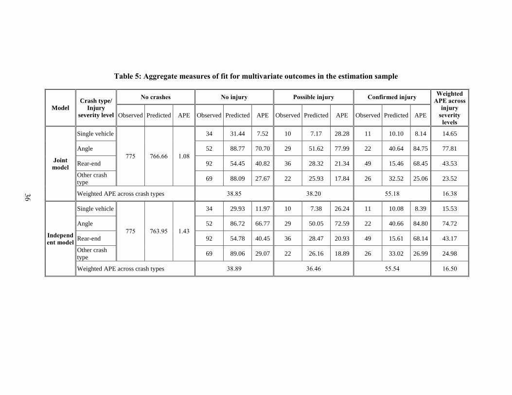
Table 5: Aggregate measures of fit for multivariate outcomes in the estimation sample

Model Crash type/

Injury

severity level

No crashes No injury Possible injury Confirmed injury Weighted

APE across injury

severity levels

Observed Predicted APE Observed Predicted APE Observed Predicted APE Observed Predicted APE

Joint model

Single vehicle

775 766.66 1.08

34 31.44 7.52 10 7.17 28.28 11 10.10 8.14 14.65

Angle 52 88.77 70.70 29 51.62 77.99 22 40.64 84.75 77.81

Rear-end 92 54.45 40.82 36 28.32 21.34 49 15.46 68.45 43.53

Other crash type

69 88.09 27.67 22 25.93 17.84 26 32.52 25.06 23.52

Weighted APE across crash types 38.85 38.20 55.18 16.38

Independent model

Single vehicle

775 763.95 1.43

34 29.93 11.97 10 7.38 26.24 11 10.08 8.39 15.53

Angle 52 86.72 66.77 29 50.05 72.59 22 40.66 84.80 74.72

Rear-end 92 54.78 40.45 36 28.47 20.93 49 15.61 68.14 43.17

Other crash type

69 89.06 29.07 22 26.16 18.89 26 33.02 26.99 24.98

Weighted APE across crash types 38.89 36.46 55.54 16.50

36

The aggregate fit measures for marginal outcomes are provided in Table 6. As expected,

the APE values are lower for these outcomes than for the multivariate outcomes (Table 5).

Overall, the count predictions from the joint model are better than the count predictions from the

independent model (the joint model, compared to the independent model, presents slightly higher

APE for event states single vehicle/no injury, angle/possible injury, angle/confirmed injury, rear-

end/confirmed injury and other crash type/possible injury). In general, the APE is lower for 0

crashes, compared to 1 and 2+ crashes, and consistently higher for angle crashes, as observed in

Table 5. The total crash count APE for 0, 1 and 2+ crashes is 1.1, 1.2 and 2.4, respectively, and

the overall weighted APE is 1.58% (2.91% for the independent model). These results show that

the joint model outperforms the traditional independent model in both disaggregate and

aggregate levels.

Table 6: Aggregate measures of fit for marginal outcomes in the estimation sample

Crash type Model Crash counts No injury Possible injury Confirmed injury

Observed Predicted APE Observed Predicted APE Observed Predicted APE

Single vehicle

Joint model

0 1297 1299.5 0.2 1335 1335.6 0.0 1331 1331.4 0.0

1 51 47.2 7.4 13 12.3 5.3 17 16.4 3.4

2+ 0 1.3 1.3 0 0.1 0.1 0 0.1 0.1

Weighted APE 0.46 0.09 0.07

Independent model

0 1297 1297.9 0.1 1335 1336.1 0.1 1331 1331.6 0.0

1 51 48.7 4.5 13 11.9 8.7 17 16.3 4.2

2+ 0 1.4 1.4 0 0.0 0.0 0 0.1 0.1


Angle

Joint model

0 1206 1215.3 0.8 1289 1265.7 1.8 1267 1282.2 1.2

1 130 119.7 8.0 53 76.4 44.2 76 62.4 17.9

2+ 12 13.0 8.7 6 5.8 3.0 5 3.4 32.7


Independent model

0 1206 1217.3 0.9 1289 1267.9 1.6 1267 1281.4 1.1

1 130 118.9 8.6 53 75.0 41.5 76 63.2 16.8

2+ 12 11.8 1.6 6 5.1 15.8 5 3.4 31.6


Rear-end

Joint model

0 1261 1262.6 0.1 1306 1302.7 0.3 1318 1322.7 0.4

1 77 81.6 5.9 40 44.1 10.2 30 24.9 17.0

2+ 10 3.9 61.3 2 1.2 38.9 0 0.4 0.4


Independent model

0 1261 1260.8 0.0 1306 1301.9 0.3 1318 1322.0 0.3

1 77 83.4 8.3 40 44.9 12.2 30 25.5 14.9

2+ 10 3.8 61.7 2 1.3 37.3 0 0.5 0.5


Other crash type

Joint model

0 1241 1216.1 2.0 1303 1306.7 0.3 1302 1296.1 0.5

1 92 123.0 33.7 43 40.2 6.5 44 50.2 14.1

2+ 15 8.9 40.7 2 1.1 44.6 2 1.7 16.4


Independent model

0 1241 1212.9 2.3 1303 1305.6 0.2 1302 1294.5 0.6

1 92 126.2 37.2 43 41.2 4.2 44 51.8 17.6

2+ 15 9.0 40.3 2 1.2 39.8 2 1.7 12.9


38

39

5.4. Elasticity Effects and Implications

Section 5.2 discussed the effects of variables on crash frequency and crash event states.

However, the coefficients do not directly provide a sense of the magnitude and direction of

effects of each variable on crash frequency at each event state. For example, the results of the

crash frequency model in Table 3 suggest that intersections controlled by stop signs tend to have

fewer crashes than signal-controlled intersections. However, the crash event state model in Table

4 shows that these intersections are more likely to present angle crashes. The positive

coefficients of Table 4, due to the positive linkage parameter, will increase the crash frequency at

intersections controlled by stop signs. Then, depending on the relative value of the crash

frequency model coefficients and the crash event state model coefficients, the overall crash

frequency may be higher or smaller than the crash frequency at signal-controlled intersections.

To clarify the effect of exogenous variable, we demonstrate the application of this model

by studying the effects of changes in all significant variables but intersection location, as this

variable does not have any policy implication. The impact on the crash frequency is estimated by

determining the percentage change in the expected number of crashes in each crash event state

(across all intersections) and for each crash event state. For the continuous variables (average

daily entering traffic volume, surface width and shoulder width), we increase the value of the

variable by 10% for each observation. For dummy variables, we first predict the number of

crashes in each crash event state for each intersection, assigning the base value of “0” for all

dummy variables characterizing each single exogenous discrete variable. Then, we change each

dummy variable to the value of “1” and, again, compute the number of crashes in each crash

event state for each intersection, and compute the percentage change. For example, consider

number and type of entering roads. We first compute the number of crashes in each crash event

state after assigning zero values for both the “three (Y-shaped)” and “four” variables for each

intersection. Because “three (T-shaped)” is the base category, this variable is already zero. Then,

we compute the number of crashes for all crash event states after changing the value of the “three

(Y-shaped)” dummy variable for each intersection from the value of zero to the value of one, and

compute the percentage difference in crash frequency with respect to the above case. The same

procedure is used for the dummy variable “four”.

Table 7 provides the results for both joint and independent models. The numbers in the

table may be interpreted as the percentage change in the crash frequency of each crash event

state due to a change in the exogenous variable. For example, the first entry in the table indicates

40

that the number of single vehicle crashes resulting in no injury is 45.68% higher for Y-shaped

intersections compared to T-shaped intersections, other characteristics being equal. Other entries

may be similarly interpreted. Several observations can be made from the results in Table 7. First,

the elasticity effects help to identify the direction and magnitude of the exogenous variables on

crash frequency. Following the example provided earlier, the table shows that intersections

controlled by stop signs, overall, have fewer crashes than signal-controlled intersections.

However, this effect is not constant across all crash event states, as angle crashes are more likely

to occur at intersections controlled by stop signs. These differences across crash event states can

be also observed for yield signs, validating the importance of considering the effect of variables

on each combination of crash types and injury severity levels. Second, Table 7 shows that Y-

shaped intersections present 44.52% more crashes than T-shaped intersections, and that this

elasticity effect is virtually the same across event states. This result suggests that a careful

investigation into the design of intersections with three entering roads, especially in terms of

skewness and visibility, can help to improve safety at rural intersections. Third, the results show

that confirmed injuries caused by angle crashes are more likely to occur in intersections

controlled by stop and yield signs. Although intersections controlled by stop and yield signs tend

to have less crashes than intersections controlled by traffic lights, the consequences of severe

crashes, in terms of property and economic loss and deaths, may require the evaluation of these

forms of traffic controls in rural intersections. Finally, the comparison between the joint and

independent model shows several differences. In particular, the effects of major roads

characteristics are clearly misestimated by the independent model. For the exogenous variables

number of lanes, surface and shoulder width, which appear only in the specification of the crash

event model and not in the crash frequency model, the change in total crash counts is zero in the

independent model. However, in the joint model the change in total crashes 18.7% for number of

lanes, and 0.75%, -0.03% and -0.09% for surface width, inside shoulder with and outside

shoulder width, respectively. These results exemplify the possible errors in policy making that

can be made when wrongly assuming that the frequency of crashes and the crash even state

outcomes of these crashes are interrelated.

Table 7: Elasticity effects -- Aggregate change in expected number of crashes

Variable Crash type/Injury

severity level

Joint model Independent model

No injury Possible injury Confirmed injury No injury Possible injury Confirmed injury


Number and type of entering roads (three (T-shaped))

Three (Y-shaped)

Single vehicle 45.68 45.76 45.74 38.50 38.78 38.74

Angle 42.68 42.35 43.33 36.92 36.50 36.74

Rear-end 45.54 45.69 45.54 38.43 38.63 38.40

Other crash type 45.33 45.50 45.64 38.26 38.27 38.47

Total number of crashes 44.52 37.80

Four

Single vehicle -24.97 -25.02 -25.02 -26.94 -27.07 -27.06

Angle -24.11 -24.04 -24.34 -26.31 -26.12 -26.23

Rear-end -24.95 -24.98 -24.93 -26.92 -27.00 -26.89

Other crash type -24.85 -24.93 -24.96 -26.83 -26.85 -26.93

Total number of crashes -24.66 -26.65

Type of traffic control (signal

light)

Stop sign

Single vehicle -75.36 -73.61 -73.39 -74.79 -75.49 -73.17

Angle 217.17 255.73 212.51 201.73 238.30 212.79

Rear-end -65.75 -75.71 -70.61 -65.09 -74.81 -69.77

Other crash type -67.35 -77.13 -75.46 -66.99 -77.24 -74.64


Yield sign

Single vehicle -57.94 -57.76 -57.52 -60.00 -60.59 -59.92

Angle 87.19 -59.06 -59.14 45.07 -62.46 -61.43

Rear-end -54.99 -58.06 -56.59 -57.75 -60.10 -58.84

Other crash type -55.17 -58.68 -57.92 -57.95 -61.07 -59.92


Center stripe or divider

Single vehicle -47.59 -47.52 -47.46 -48.92 -48.97 -48.89

Angle -47.55 -47.63 -47.56 -49.08 -49.13 -48.96

Rear-end -47.57 -47.48 -47.62 -48.92 -48.91 -48.96

Other crash type -47.53 -47.83 -47.56 -48.90 -49.11 -48.90


Other traffic control

Single vehicle -27.37 -27.33 -27.28 -31.39 -31.43 -31.36

Angle -27.33 -27.38 -27.35 -31.50 -31.54 -31.41

Rear-end -27.36 -27.30 -27.40 -31.39 -31.38 -31.42

Other crash type -27.33 -27.53 -27.35 -31.37 -31.53 -31.37


No traffic control or

minimal traffic control

Single vehicle -69.24 -69.16 -69.12 -70.30 -70.34 -70.29

Angle -69.25 -69.34 -69.24 -70.49 -70.54 -70.36

Rear-end -69.23 -69.14 -69.28 -70.31 -70.30 -70.34

Other crash type -69.20 -69.52 -69.22 -70.29 -70.50 -70.29


41

Table 7: Elasticity effects -- Aggregate change in expected number of crashes (cont.)

Variable Crash type/Injury severity

level

Joint model Independent model

No injury Possible injury

Confirmed injury

No injury Possible injury

Confirmed injury


Number of lanes (two)

Four

Single vehicle -17.24 -17.76 -16.50 -26.66 -28.78 -25.96

Angle -16.05 184.45 374.27 -30.68 131.50 258.71

Rear-end -9.96 -17.79 -14.28 -20.72 -27.01 -24.11

Other crash type -11.17 -16.25 -17.09 -21.82 -24.05 -26.29


Traffic conditions

Average daily entering traffic

volume (veh/day)

Single vehicle -1.08 -0.99 -1.07 -0.52 -0.51 -0.51

Angle -1.07 -1.13 -0.97 -0.38 -0.41 -0.38

Rear-end -1.00 -1.03 -1.04 -0.41 -0.51 -0.47

Other crash type -1.00 3.25 -1.08 -0.43 4.05 -0.52


Surface width (feet)

Single vehicle -0.17 -0.01 -0.13 -0.58 -0.43 -0.58

Angle 13.04 -0.15 -19.62 11.58 -1.05 -19.38

Rear-end -0.11 -0.11 -0.08 -0.57 -0.52 -0.51

Other crash type -0.10 -0.16 -0.11 -0.56 -0.72 -0.53



Inside shoulder

Single vehicle 0.08 0.13 -3.49 0.12 0.16 -3.61

Angle 0.03 0.04 0.05 0.05 0.06 0.07

Rear-end 0.05 0.07 0.10 0.09 0.11 0.15

Other crash type 0.04 0.08 0.07 0.08 0.12 0.12

Total number of crashes -0.03 0.00

Outside shoulder

Single vehicle 0.20 -3.23 0.20 0.34 -3.41 0.33

Angle 0.09 0.11 0.13 0.15 0.18 0.20

Rear-end 0.10 -2.56 0.19 0.22 -2.62 0.33

Other crash type 0.10 0.20 21.47 0.23 0.35 0.34

Total number of crashes -0.09 0.00

42

43

CHAPTER 6: CONCLUSIONS

This report has proposed an econometric multivariate structure for crash frequency analysis that

combines a total count model with a discrete choice model that allocates the total crash count to

different combinations of crash type and injury severity levels (referred as crash event states).

This approach simultaneously (a) recognizes the linkage between the combinations of crash type

and injury severity and the total crash count by incorporating the effect of the crash event state’s

errors on the total crash count, which is critical to recognize the full econometric jointness of the

two outcomes, (b) uses a flexible MNP structure for the discrete choice model to accommodate

unobserved heterogeneity in the effects of contributing factors, (c) uses new results regarding the

distribution of the maximum of multivariate normally distributed random variables (with a

general covariance matrix) as well as its stochastic affine transformations (see Bhat et al., 2014),

and (d) employs a latent variable framework for modeling the total crash count that, at once,

enables the linkage of the discrete choice model and crash count model, recognizes the presence

of unobserved heterogeneity, and accommodates excess of zeros (or excess number of any count

value) without the need for zero-inflated or hurdle devices. The resulting joint crash frequency -

crash event state model is estimated using a relatively straightforward-to-implement composite

marginal likelihood (CML) inference approach. To our knowledge, this model is the first

formulation of its kind to be proposed and applied in the safety analysis literature.

The proposed model is applied to model crash frequency by combinations of crash type

and severity injury on rural intersections in central Texas, using the crash incident files

maintained by the Texas Department of Transportation. Crash type was classified in four levels

(single vehicle, angle, rear-end and other crash type) and injury severity in three levels (no

injury, possible injury and confirmed injury), accounting for 12 crash type/injury level

combinations. The empirical results clearly reveal the benefits, both in terms of capturing

flexibility in variable effects and data fit, to adopting the proposed structure. From a substantive

standpoint, the results underscore the important effects of intersection design and major road

characteristics in determining the number of crashes in each category.

45

REFERENCES

Aguero-Valverde, J and Jovanis, P P, 2009, “Bayesian Multivariate Poisson Lognormal Models

for Crash Severity Modeling and Site Ranking” Transportation Research Record: Journal of the Transportation Research Board 2136(-1) 82–91.

Alfò, M and Maruotti, A, 2010, “Two-part regression models for longitudinal zero-inflated count data” Canadian Journal of Statistics 38(2) 197–216.

Anastasopoulos, P C, Shankar, V N, Haddock, J E, and Mannering, F L, 2012, “A multivariate tobit analysis of highway accident-injury-severity rates” Accident Analysis & Prevention 45 110–119.

Awondo, S N, Egan, K J, and Dwyer, Dary F, 2011, “Increasing Beach Recreation Benefits by Using Wetlands to Reduce Contamination” Marine Resource Economics 26(1) 1–15.

Bagdadi, O, 2013, “Estimation of the severity of safety critical events” Accident Analysis & Prevention 50 167–174.

Bai, L and Fan, J J, 2012, “Multivariate Poisson-Lognormal Regression for Crash Prediction of Different Types on Freeways Diverge Areas” Applied Mechanics and Materials 236-237 683–688.

Bhat, C R, 2011, “The maximum approximate composite marginal likelihood (MACML) estimation of multinomial probit-based unordered response choice models” Transportation Research Part B 45(7) 923–939.

Bhat, C R, Paleti, R, and Castro, M, 2014, “A new utility-consistent econometric approach to multivariate count data modeling" Journal of Applied Econometrics, forthcoming.

Bullough, J D, Donnell, E T, and Rea, M S, 2013, “To illuminate or not to illuminate: Roadway lighting as it affects traffic safety at intersections” Accident Analysis & Prevention 53 65–77.

Burda, M, Harding, M, and Hausman, J, 2012, “A Poisson mixture model of discrete choice” Journal of Econometrics 166(2) 184–203.

Castro, M, Paleti, R, and Bhat, C R, 2012, “A latent variable representation of count data models to accommodate spatial and temporal dependence: Application to predicting crash frequency at intersections” Transportation Research Part B 46(1) 253–272.

Chib, S and Winkelmann, R, 2001, “Markov Chain Monte Carlo Analysis of Correlated Count Data” Journal of Business & Economic Statistics 19(4) 428–435.

Chiou, Y-C and Fu, C, 2013, “Modeling crash frequency and severity using multinomial-generalized Poisson model with error components” Accident Analysis & Prevention 50 73–82.

Cox, D R and Reid, N, 2004, “A note on pseudolikelihood constructed from marginal densities” Biometrika 91(3) 729–737.

El-Basyouny, K and Sayed, T, 2009, “Collision prediction models using multivariate Poisson-lognormal regression” Accident Analysis & Prevention 41(4) 820–828.

El-Basyouny, K and Sayed, T, 2010, “A method to account for outliers in the development of safety performance functions” Accident Analysis & Prevention 42(4) 1266–1272.

46

Elvik, R, 2011, “Assessing causality in multivariate accident models” Accident Analysis & Prevention 43(1) 253–264.

FHWA, 2005, “Crash cost estimates by maximum police-reported injury severity within selected crash geometries” Federal Highway Administration FHWA HRT 05 051, http://www.fhwa.dot.gov/publications/research/safety/05051/.

Godambe, V P, 1960, “An optimum property of regular maximum likelihood estimation” The Annals of Mathematical Statistics 31(4) 1208–1211.

Haque, M M, Chin, H C, and Huang, H, 2010, “Applying Bayesian hierarchical models to examine motorcycle crashes at signalized intersections” Accident Analysis & Prevention 42(1) 203–212.

Hausman, J A, Leonard, G K, and McFadden, D, 1995, “A utility-consistent, combined discrete choice and count data model Assessing recreational use losses due to natural resource damage” Journal of Public Economics 56(1) 1–30.

Herriges, J A, Phaneuf, D J, and Tobias, J L, 2008, “Estimating demand systems when outcomes are correlated counts” Journal of Econometrics 147(2) 282–298.

Huang, H, Chin, H C, and Haque, M M, 2008, “Severity of driver injury and vehicle damage in traffic crashes at intersections: A Bayesian hierarchical analysis” Accident Analysis & Prevention 40(1) 45–54.

Jonsson, T, Ivan, J N, and Zhang, C, 2007, “Crash Prediction Models for Intersections on Rural Multilane Highways: Differences by Collision Type” Transportation Research Record: Journal of the Transportation Research Board 2019(-1) 91–98.

Kim, D-G, Lee, Y, Washington, S, and Choi, K, 2007, “Modeling crash outcome probabilities at rural intersections: Application of hierarchical binomial logistic models” Accident Analysis & Prevention 39(1) 125–134.

Lee, A H, Wang, K, Scott, J A, Yau, K K W, and McLachlan, G J, 2006, “Multi-level zero-inflated Poisson regression modelling of correlated count data with excess zeros” Statistical Methods in Medical Research 15(1) 47–61.

Lindsay, B G, 1988, “Composite likelihood methods” Contemporary Mathematics 80(1) 221–239.

Lord, D, 2006, “Modeling motor vehicle crashes using Poisson-gamma models: Examining the effects of low sample mean values and small sample size on the estimation of the fixed dispersion parameter” Accident Analysis & Prevention 38(4) 751–766.

Lord, D and Mannering, F, 2010, “The statistical analysis of crash-frequency data: A review and assessment of methodological alternatives” Transportation Research Part A 44(5) 291–305.

Ma, J, Kockelman, K M, and Damien, P, 2008, “A multivariate Poisson-lognormal regression model for prediction of crash counts by severity, using Bayesian methods” Accident Analysis & Prevention 40(3) 964–975.

Mannering, F L and Hamed, M M, 1990, “Occurence, frequency, and duration of commuters’ work-to-home departure delay” Transportation Research Part B 24(2) 99–109.

Mitra, S and Washington, S, 2007, “On the nature of over-dispersion in motor vehicle crash prediction models” Accident Analysis & Prevention 39(3) 459–468.

47

Molenberghs, G and Verbeke, G, 2005 Models for discrete longitudinal data (Springer, New York ; London).

Narayanamoorthy, S, Paleti, R, and Bhat, C R, 2013, “On accommodating spatial dependence in bicycle and pedestrian injury counts by severity level” Transportation Research Part B 55 245–264.

NHTSA, 2011, “Fatality analysis reporting system (FARS) query system” National Highway Traffic Safety Administration, http://www-fars.nhtsa.dot.gov/QueryTool/QuerySection/SelectYear.aspx.

NHTSA, 2013a, “Early estimate of motor vehicle traffic fatalities in 2012” National Center for Statistics and Analysis, U.S. Department of Transportation DOT HS 811 741, http://www-nrd.nhtsa.dot.gov/Pubs/811741.pdf.

NHTSA, 2013b, “Traffic safety facts 2011: FARS/GES annual report (final edition)” National Center for Statistics and Analysis, U.S. Department of Transportation DOT HS 811 754, http://www-nrd.nhtsa.dot.gov/Pubs/811754AR.pdf.

NVSR, 2012, “Deaths: Preliminary data for 2011” National Vital Statistics Reports 61(6), http://www.cdc.gov/nchs/data/nvsr/nvsr61/nvsr61_06.pdf.

Pace, L, Salvan, A, and Sartori, N, 2011, “Adjusting composite likelihood ratio statistics” Statistica Sinica 21(1) 129–148.

Park, E S and Lord, D, 2007, “Multivariate Poisson-Lognormal Models for Jointly Modeling Crash Frequency by Severity” Transportation Research Record: Journal of the Transportation Research Board 2019(-1) 1–6.

Pei, X, Wong, S C, and Sze, N N, 2011, “A joint-probability approach to crash prediction models” Accident Analysis & Prevention 43(3) 1160–1166.

Polanis, S F, 2002, “Right-angle crashes and late-night/early-morning flashing operation: 19 case studies” ITE Journal 72(4), 26–28.

Qin, X, Ivan, J N, and Ravishanker, N, 2004, “Selecting exposure measures in crash rate prediction for two-lane highway segments” Accident Analysis & Prevention 36(2) 183–191.

Qin, X, Ng, M, and Reyes, P E, 2010, “Identifying crash-prone locations with quantile regression” Accident Analysis & Prevention 42(6) 1531–1537.

Retting, R A, Weinstein, H B, and Solomon, M G, 2003, “Analysis of motor-vehicle crashes at stop signs in four U.S. cities” Journal of Safety Research 34(5) 485–489.

Rouwendal, J and Boter, J, 2009, “Assessing the value of museums with a combined discrete choice/count data model” Applied Economics 41(11) 1417–1436.

Savolainen, P T, Mannering, F L, Lord, D, and Quddus, M A, 2011, “The statistical analysis of highway crash-injury severities: A review and assessment of methodological alternatives” Accident Analysis & Prevention 43(5) 1666–1676.

Shankar, V, Mannering, F, and Barfield, W, 1995, “Effect of roadway geometrics and environmental factors on rural freeway accident frequencies” Accident Analysis & Prevention 27(3) 371–389.

48

Sifrit, K J, 2011, “Drivers in their 60s, 70s and older: Analyses of FARS and GES data” NHTSA’s Office of Behavioral Safety Research, http://crag.uab.edu/safemobility/Presentations/2011%20Kathy%20Sifrit.pdf.

Srinivasan, R, Council, F, Lyon, C, Gross, F, Lefler, N, and Persaud, B, 2008, “Safety Effectiveness of Selected Treatments at Urban Signalized Intersections” Transportation Research Record: Journal of the Transportation Research Board 2056(-1) 70–76.

Terza, J V and Wilson, P W, 1990, “Analyzing frequencies of several types of events: A mixed multinomial-Poisson approach” The Review of Economics and Statistics 72(1) 108–115.

Varin, C and Vidoni, P, 2008, “Pairwise Likelihood Inference for General State Space Models” Econometric Reviews 28(1-3) 170–185.

Venkataraman, N, Ulfarsson, G F, and Shankar, V N, 2013, “Random parameter models of interstate crash frequencies by severity, number of vehicles involved, collision and location type” Accident Analysis & Prevention 59 309–318.

Wang, C, Quddus, M A, and Ison, S G, 2011, “Predicting accident frequency at their severity levels and its application in site ranking using a two-stage mixed multivariate model” Accident Analysis & Prevention 43(6) 1979–1990.

Xu, X and Reid, N, 2011, “On the robustness of maximum composite likelihood estimate” Journal of Statistical Planning and Inference 141(9) 3047–3054.

Ye, X, Pendyala, R M, Shankar, V, and Konduri, K C, 2013, “A simultaneous equations model of crash frequency by severity level for freeway sections” Accident Analysis & Prevention 57 140–149.

Ye, X, Pendyala, R M, Washington, S P, Konduri, K, and Oh, J, 2009, “A simultaneous equations model of crash frequency by collision type for rural intersections” Safety Science 47(3) 443–452.

Yi, G Y, Zeng, L, and Cook, R J, 2011, “A robust pairwise likelihood method for incomplete longitudinal binary data arising in clusters” Canadian Journal of Statistics 39(1) 34–51.

Yu, R and Abdel-Aty, M, 2013, “Multi-level Bayesian analyses for single- and multi-vehicle freeway crashes” Accident Analysis & Prevention 58 97–105.

Zhao, Y and Joe, H, 2005, “Composite likelihood estimation in multivariate data analysis” Canadian Journal of Statistics 33(3) 335–356.

technical report documentation page 1. report no. 2 ... · (2014) to formulate and ... crash...

Documents