technical report 93 monitoring of the freshwater ... · in 'ohe'o are unknown. limited...
TRANSCRIPT

COOPERATIVE NATIONAL PARK RESOURCES STUDIES UNIT UNIVERSITY OF HAWAI'I AT MANOA
Department o f Botany 3190 Maile Way
Honolulu, Hawai'i 96822 (808) 956-8218
Technical Report 93 MONITORING OF THE
FRESHWATER AMPHIDROMOUS POPULATIONS OF THE 'OHE'O GULCH STREAM SYSTEM AND
PUA'ALU'U STREAM, HALEAKALA NATIONAL PARK Marc H. Hodges
Research Station Haleakalii National Park
P. 0. Box 369 Makawao, HI 96768
UNIVERSITY OF HAWAI'I AT MANOA NATIONAL PARK SERVICE
Cooperative Agreement CA 8032-2-0001
December 1994

TABLE OF CONTENTS ...
. . . . . . . . . . . . . . . . . . . . . . . . . . . . . . . . . . . . . . . . . . . . . . . . . . . . . . . . . . . . . . . . . . . . . . . . . . . . . . . . . . . . . . . . . . . . . . . . . . . . . . . . . . . . . . . . . LIST OF FIGURES I I I
............................................................................................................................ ABSTRACT iv
..................................................................................................................... LNTRODUCTION 1 . . Hawallan Streams and Strcam Life . . . . . . . . . . . . . . . . . . . . . . . . . . . . . . . . . . . . . . . . . . . . . . . . . . . . . . . . . . . . . . . . . . . . . . . . . . . . . . . . . . . . . . . . . . 1
.......................................................................................................................... 'Ohe'o Gulch 1 .............................................................................................................................. Study Area 1
... . . . . . . . . . . . . . . . . . . . . . . . . . . . . . . . . . . . . . . . . . . . . . . . . . . . . . . . . . . . . . . . . . . . . . . . . . . . . . . . . . . . . . . . . . . . . . . . . . . . . . . . . . . . . . . . Physical Setting 1 3 Morphology and Hydrology . . . . . . . . . . . . . . . . . . . . . . . . . . . . . . . . . . . . . . . . . . . . . . . . . . . . . . . . . . . . . . . . . . . . . . . . . . . . . . . . . . . . . . . . . . . . . . . &
. . . . . . . . . . . . . . . . . . . . . . . . . . . . . . . . . . . . . . . . . . . . . . . . . . . . . . . . . . . . . . . . . . . . . . . . . . . . . . . . . . . . . . . . . . . . . . . . . . Water Quality Information 2 . . . . . . . . . . . . . . . . . . . . . . . . . . . . . . . . . . . . . . . . . . . . . . . . . . . . . . . . . . . . . . . . . . . . . . . . . . . . . . . . . . . . . . . . . . . . . . . . . . . . . . . . Discharge Infor~nation 2
METHODOL. OGY . . . . . . . . . . . . . . . . . . . . . . . . . . . . . . . . . . . . . . . . . . . . . . . . . . . . . . . . . . . . . . . . . . . . . . . . . . . . . . . . . . . . . . . . . . . . . . . . . . . . . . . . . . . . . . . . . . . 3 . . . . . . . . . . . . . . . . . . . . . . . . . . . . . . . . . . . . . . . . . . . . . . . . . . . . . . . . . . . . . . . . . . . . . . . . . . . . . . . . . . . . . . . . . . . . . . . . . . . . . . . . . . . . . . . . . . . . . . Station Layout 3
Survey Methods ............ ..... . . . . . . . . . . . . . . . . . . . . . . . . . . . . . . . . . . . . . . . . . . . . . . . . . . . . . . . . . . . . . . . . . . . . . . . . . . . . . . . . . . . . . . . . . . . . . . . 3 Direct Observation ....................................................................................................... 3
. . . . . . . . . . . . . . . . . . . . . . . . . . . . . . . . . . . . . . . . . . . . . . . . . . . . . . . . . . . . . . . . . . . . . . . . . . . . . . . . . . . . . . . . . . . . . . . . Trapping . . . . . . . . . . . . . . . . . . . .. 6 Pua'alu'u Stream . . . . . . . . . . . . . . . . . . . . . . . . . . . . . . . . . . . . . . . . . . . . . . . . . . . . . . . . . . . . . . . . . . . . . . . . . . . . . . . . . . . . . . . . . . . . . . . . . . . . . . . . . . . . . . . . 7
. . . . . . . . . . . . . . . . . . . . . . . . . . . . . . . . . . . . . . . . . . . . . . . . . . . . . . . . . . . . . . . . . . . . . . . . . . . . . . . Survey Design and Statistical Analysis 8
. . . . . . . . . . . . . . . . . . . . . . . . . . . . . . . . . . . . . . . . . . . . . . . . . . . . . . . . . . . . . . . . . . . . . . . . . . . . . . . . . . . . . . . . . . . . . . . . . . . . . . . . . . . . . . . . . . . . . . . . . . . . . . . . . RESULTS 9 The 'o'opu in 'Ohe'o . . . . . . . . . . . . ..,....... . ! ....... .. .... . . . . . . . . . . . . . . . . . . . . . . . . . . . . . . . . . . . . . . . . . . . . . . . . . . . . . . . . . . . . . . . . . . . 9
Temporal Differences . . . . . . . . . . . . . . . . . . . . . . . . . . . . . . . . . . . . . . . . . . . . . . . . . . . . . . . . . . . . . . . . . . . . . . . . . . . . . . . . . . . . . . . . . . . . . . . . . . . . . . . . . 9 . . . . . . . . . . . . . . . . . . . . . . . . . . . . . . . . . . . . . . . . . . . . . . . . . . . . . . . . . . . . . . . . . . . . . . . . . . . . . . . . . . . . . . . . . . . . . . . . . . . . . . . . . . . Spatial Differences 1 1
. . . . . . . . . . . . . . . . . . . . . . . . . . . . . . . . . . . . . . . . . . . . . . . . . . . . . . . . . . . . . . . . . . . . . . . . . . . . . . . . . . . . . . . . . . . . . . . . . . Additional Observations I2 '- . '
. . . . . . . . . . . . . . . . . . . . . . . . . . . . . . . . . . . . . . . . . . . . . . . . . . . . . . . . . . . . . . . . . . . . . . . . . . . . . . . . . . . . . . . . . . . . . . . . . . . . . The opae rn Ohe'o 14 . . Temporal D~flerences . . . . . . . . . . . . . . . . . . . . . . . . . . . . . . . . . . . . . . . . . . . . . . . . . . . . . . . . . . . . . . . . . . . . . . . . . . . . . . . . . . . . . . . . . . . . . . . . . . . . . . 14
. . . . . . . . . . . . . . . . . . . . . . . . . . . . . . . . . . . . . . . . . . . . . . . . . . . . . . . . . . . . . . . . . . . . . . . . . . . . . . . . . . . . . . . . . . . . . . . . . . . . . . . . . . Spatial Dit'ferences 16 . . . . . . . . . . . . . . . . . . . . . . . . . . . . . . . . . . . . . . . . . . . . . . . . . . . . . . . . . . . . . . . . . . . . . . . . . . . . . . . . . . . . . . . . . . . . . . . . . Additional Observations 16
. . . . . . . . . . . . . . . . . . . . . . . . . . . . . . . . . . . . . . . . . . . . . . . . . . . . . . . . . . . . . . . . . . . . . . . . . . . . . . . . . . . . . . . . . . . . . . . . . . . . . . . . . . . The hihiwa~ ~n 'Ohe'o 16
. . . . . . . . . . . . . . . . . . . . . . . . . . . . . . . . . . . . . . . . . . . . . . . . . . . . . . . . . . . . . . . . . . . . . . . . . . . . . . . . . . . . . . . The M . /or in 'Ohe'o ... ...: 16 . .
. . . . . . . . . . . . . . . . . . . . . . . . . . . . . . . . . . . . . . . . . . . . . . . . . . . . . . . . . . . . . . . . . . . . . . . . . . . . . . . . . . . . . . . . . . . . . . . . . . . . . . . Temporal D~fferences 16 . . . . . . . . . . . . . . . . . . . . . . . . . . . . . . . . . . . . . . . . . . . . . . . . . . . . . . . . . . . . . . . . . . . . . . . . . . . . . . . . . . . . . . . . . . . . . . . . . . . . . . . . . . . Spatial Dif'ferences 17
. . . . . . . . . . . . . . . . . . . . . . . . . . . . . . . . . . . . . . . . . . . . . . . . . . . . . . . . . . . . . . . . . . . . . . . . . . . . . . . . . . . . . . . . . . . . . . . . . . . Additional Observations 18 . . . . . . . . . . . . . . . . . . . . . . . . . . . . . . . . . . . . . . . . . . . . . . . . . . . . . . . . . . . . . . . . . . . . . . . . . . . . . . . . . . . . . . . . . . . . . . . . . . . . . . . . The 'o'opu in Pua'alu'u 21 -
.. . . . . . . . . . . . . . . . . . . . . . . . . . . . . . . . . . . . . . . . . . . . . . . . . . . . . . . . . . . . . . . . . . . . . . . . . . . . . . . . . . . . . . . . . . . . . . . . . . . . . . . . . The 'opae in Pua'alu'u 21 . .
. . . . . . . . . . . . . . . . . . . . . . . . . . . . . . . . . . . . . . . . . . . . . . . . . . . . . . . . . . . . . . . . . . . . . . . . . . . . . . . . . . . . . . . . . . . . . . . . . . . . . . . The hihiwa~ ~n Pua'alu'u 22 . . . . . . . . . . . . . . . . . . . . . . . . . . . . . . . . . . . . . . . . . . . . . . . . . . . . . . . . . . . . . . . . . . . . . . . . . . . . . . . . . . . . . . . . . . . . . . . . . . . . . . 'Ohe'o vs . PuaLalu'u 22
. . . . . . . . . . . . . . . . . . . . . . . . . . . . . . . . . . . . . . . . . . . . . . . . . . . . . . . . . . . . . . . . . . . . . . . . . . . . . . . . . . . . . . . . . . . . . . . . . . . . . . . . . . . . . . . . . . . . DISCkJSSION 22 . . . . . . . . . . . . . . . . . . . . . . . . . . . . . . . . . . . . . . . . . . . . . . . . . . . . . . . . . . . . . . . . . . . . . . . . . . . . . . . . . . . . . . . . . . . . . . . . . . . . . The 'o'opu in 'Ohe'o 22
. . . . . . . . . . . . . . . . . . . . . . . . . . . . . . . . . . . . . . . . . . . . . . . . . . . . . . . . . . . . . . . . . . . . . . . . . . . . . . . . . . . . . . . . . . . . . . . . . . . . . . . . . . . . . . . . . . . . . . . . . Method 22 . . . . . . . . . . . . . . . . . . . . . . . . . . . . . . . . . . . . . . . . . . . . . . . . . . . . . . . . . . . . . . . . . . . Within-stream distribution of 'o'opu species 22

Generally low abundance but significant ala~no'o . . . . . . . . . . . . . . . . . . . . . . . . . . . . . . . . . . . . . . . . . . . . . . . . . . . . . . . . . . . . . 23 The 'tipae in 'Ohe'o .............................................................................................................. 23 The hihiwai in 'Ohe'o .......................................................................................................... 23 The M . lor in 'Ohe'o ............................................................................................................. 23
Abundance ....................................................................................................................... 23 Incidence of 'black-spotted' disease . . . . . . . . . . . . . . . . . . . . . . . . . . . . . . . . . . . . . . . . . . . . . . . . . . . . . . . . . . . . . . . . . . . . . . . . . . . . . . . . . . . 23 Effect of M . ltrr on native a~nphidromous huna . . . . . . . . . . . . . . . . . . . . . . . . . . . . . . . . . . . . . . . . . . . . . . . . . . . . . . . . . . . . . . . . 23 Control ............................................................................................................................ 23
Additional Observations in 'Ohe'o ........................................................................................ 24 Does the present vis~lal survey salnpling strategy produce
adequate statistical power? .................................................................................... 24 Generally low abundance .................................................................................................. 26 Populations are fairly stable over survey period ............................ .. .............................. 27 Pua'alu'u and 'Ohe'o are good study sites . . . . . . . . . . . . . . . . . . . . . . . . . . . . . . . . . . . . . . . . . . . . . . . . . . . . . . . . . . . . . . . . . . . . . . . . 27
SUMMARY . . . . . . . . . . . . . . . . . . . . . . . . . . . . . . . . . . . . . . . . . . . . . . . . . . . . . . . . . . . . . . . . . . . . . . . . . . . . . . . . . . . . . . . . . . . . . . . . . . . . . . . . . . . . . . . . . . . . . . . . . . . . . 27 Future Research . . . . . . . . . . . . . . . . . . . . . . . . . . . . . . . . . . . . . . . . . . . . . . . . . . . . . . . . . . . . . . . . . . . . . . . . . . . . . . . . . . . . . . . . . . . . . . . . . . . . . . . . . . . . . . . . . . . 27
LITERATURE CITED
ACKNOWLEDGEMENTS . . . . . . . . . . . . . . . . . . . . . . . . . . . . . . . . . . . . . . . . . . . . . . . . . . . . . . . . . . . . . . . . . . . . . . . . . . . . . . . . . . . . . . . . . . . . . . . . 28
APPENDICES Appendix I . Raw data from 'Ohe'o
Number of 'o'opu recorded . . . . . . . . . . . . . . . . . . . . . . . . . . . . . . . . . . . . . . . . . . . . . . . . . . . . . . . . . . . . . . . . . . . . . . . . . . . . . . . . . . . . . . . . . . . . . . 29 Size classes of 'o'opu recorded . . . . . . . . . . . . . . . . . . . . . . . . . . . . . . . . . . . . . . . . . . . . . . . . . . . . . . . . . . . . . . . . . . . . . . . . . . . . . . . . . . . . . . 33 - < - Number of opae recorded . . . . . . . . . . . . . . . . . . . . . . . . . . . . . . . . . . . . . . . . . . . . . . . . . . . . . . . . . . . . . . . . . . . . . . . . . . . . . . . . . . . . . . . . . . . . . . . 37 Size classes of '5pae recorded . . . . . . . . . . . . . . . . . . . . . . . . . . . . . . . . . . . . . . . . . . . . . . . . . . . . . . . . . . . . . . . . . . . . . . . . . . . . . . . . . . . . . . . . . 41 Number, size classes, and number of egg cases of hihiwai recorded . . . . . . . . . . . . . . . . . . . . . . . . . . . . . . . . 43 Number, size classes, and additional characteristics of M . krr recorded . . . . . . . . . . . . . . . . . . . . . . . . . . . . . 45
Appendix 11 . Raw data from Pua'alu'i~ ' L < Number of o opu recorded . . . . . . . . . . . . . . . . . . . . . . . . . . . . . . . . . . . . . . . . . . . . . . . . . . . . . . . . . . . . . . . . . . . . . . . . . . . . . . . . . . . . . . . . . . . . . 53
Size classes of 'o'opu recorded . . . . . . . . . . . . . . . . . . . . . . . . . . . . . . . . . . . . . . . . . . . . . . . . . . . . . . . . . . . . . . . . . . . . . . . . . . . . . . . . . . . . 55 Number of 'Gpae recortlccl . . . . . . . . . . . . . . . . . . . . . . . . . . . . . . . . . . . . . . . . . . . . . . . . . . . . . . . . . . . . . . . . . . . . . . . . . . . . . . . . . . . . . . . . . 57 Number, size classes, and number of egg cases ot'llihiwai recorded . . . . . . . . . . . . . . . . . . . . . . . . . . . . . . . . 50
. Appendix 111 Code for resampling program . . . . . . . . . . . . . . . . . . . . . . . . . . . . . . . . . . . . . . . . . . . . . . . . . . . . . . . . . . . . . . . . . . . . . . . . . 61
Fig . 1 . Study area ..................................................................................................................... v Fig . 2 . Station locations (A) ..................................................................................................... 3 Fig . 3 . Station locations (B) ...................................................................................................... 4 Fig . 4 . Use of Cartesian coordinate system to define quadrat locations ...................................... 5 Fig . 5 . Adaptation of Cartesian coordinate system to deep pools .............. .. ........................... 5 Fig . 6 . Diagram of wire mesh trap used for Mcrcrohrochiwm lor . . . . . . . . . . . . . . . . . . . . . . . . . . . . . . . . . . . . . . . . . . . . . . . . 7 Fig . 7 . Frequency distribution of the number of 'o'opu per quadrat ........................................... 9 Fig . 8 . Mean number of 'o'opu recorded at each station .......................................................... 10 Fig . 9 . Size classes of 'o'opu recorded .................................................................................... 1 1 Fig . 10 . Size classes of 'o'opu recorded during the first survey .............................................. 12 Fig . 1 1 . Size classes of 'o'opu recorded during the second survey ............................................. 12 Fig . 12 . Means of counts of 'o'opu made by each observer . . . . . . . . . . . . . . . . . . . . . . . . . . . . . . . . . . . . . . . . . . . . . . . . . . . . . . . 13 Fig . 13 . Frequency distribution of the number of 'Gpae pcr quadrat . . . . . . . . . . . . . . . . . . . . . . . . . . . . . . . . . . . . . . . . . . . 13 Fig . 14 . Distribution of 'Cpae along 'Ohe'o . . . . . . . . . . . . . . . . . . . . . . . . . . . . . . . . . . . . . . . . . . . . . . . . . . . . . . . . . . . . . . . . . . . . . . . . . . . . . . 14 Fig . 1 5 . Post-orbital carapace lengths of 'Gpae , . . . . . . . . . . . . . . . . . . . . . . . . . . . . . . . . . . . . . . . . . . . . . . . . . . . . . . . . . . . . . . . . . . . . . . . . 14 Fig . 16 . Post-orbital carapacc lengths '6pae at g a ~ h station . . . . . . . . . . . . . . . . . . . . . . . . . . . . . . . . . . . . . . . . . . . . . . . . . . . . . . 15 Fig . 17 . Number of M . lcw trapped (luring each survey . . . . . . . . . . . . . . . . . . . . . . . . . . . . . . . . . . . . . . . . . . . . . . . . . . . . . . . . . . . . . I 7 Fig . 18 . Lengths and related statistics of M . far trapped during each sulvey . . . . . . . . . . . . . . . . . . . . . . . . . . . . . . 18 Fig . 19 . Size frequency distribution of M . lcrr trapped during each survey at each region . . . . . . . . . . . 19 Fig . 20 . Lengths of M . Inr exhibiting symptoms of 'black-spotted' disease ................................. 20 Fig . 2 1 . Densities of 'o'opu and '6pae in lower Pua'alu'u and lower 'Ohe'o ............................. 21 Fig . 22 . Densities of hihiwai and hihiwai eggs in lower Pua'alu'u and lower 'Ohe'o . . . . . . . . . . . . . . . . . . 22 Fig . 23 . Non-centrality parameter as a function of the number of quadrats per station ('6pae) . . . 25 Fig . 24 . Non-centrality parameter as a fimction of the nu~vber of quadrats per station ('o'opu) . 26

ABSTRACT
Conservation and management of Hawai'i's native freshwater-amphidromous fishes, crustaceans, and gastropods is hindered by a lack of biological information. A one year project was begun at 'Ohe'o Gulch, Haleaka15 National Park in November, 1992 to develop population survey methodologies for application at 'Ohe'o and other streams, to establish a baseline of population information at 'Ohe'o, and to gather population data which could be compared to populations elsewhere. Direct observation quadrat methods were used to survey the populations of 'o'opu (Lenfipes concolor, Sicyopterous stirnpsoni, and Awaous guamcnsis), '6pae kuahiwi (Atya bisulcata), and hihiwai (Neritina gmnosa). Trapping was used to survey the alien prawn Macrobrachiurn lar. During the project the 'o'opu and '6pae populations were surveyed twice each. Hihiwai and M. lar were surveyed three and four times each respectively. IIabitat quality appeared poor overall, but good in some upper segments of the stream system. The method developed for 'o'opu provided consistent results between observers and through time. Methods for the other species also provided good results. In the cases of 'o'opu and '6pae, numerical resampling of survey data dcmonstratcd that statistical power to detect temporal changes in overall density is likely to bc enhanced by using fewcr quadrats per station and a greater number of stations in subsequent surveys. The overall size frequencies and the within- stream distribution of average sizes of 'o'opu, '6pae, and M. lar were fairly stable. The within-stream species distribution of 'o'opu conformed to expectations and was also stable. In comparison with other streams in pristine areas of Hawai'i, 'o'opu and 'Zipae abundance was generally low. I Iowcver, 'o'opu 'alamo'o were locally abundant and individual 'alamo'o were very large in some areas. E Iihiwai were almost non-existent and appear to have declined in abundance since a prior survey two decades ago. M. lar were abundant and exhibited symptoms of 'black-spotted' disease. Other demographic characteristics of these species were analyzed. The causes of the observed low native faunal abundance in 'Ohe'o are unknown. Limited surveys were also carried out in next-door Pua'alu'u Stream. Within- stream species distribution differed between lower 'Ohe'o and the lower reach of Pua'alu'u. Such difference may be attributed to differing hydrology and geomorphology. Population monitoring in 'Ohe'o should continue and include monitoring of reproduction and recruitment via larval trapping at the terminus. Such monitoring might be conducted in conjunction with an M. lar control program.

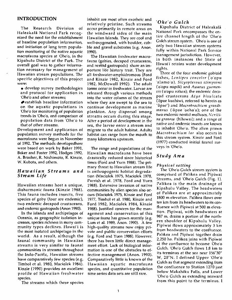
INTRODUCTION
The Research Division of Haleakal i National Park recog- nized the need for the establishment of baseline population information, and initiation of long term popula- tion monitoring of the native aquatic macrofauna species at 'Ohe'o, in the Kipahulu District of the Park. The overall goal was to gather informa- tion necessary for management of Hawaiian stream populations. The specific objectives of this project were:
0 develop survey methodologies and protocol for application in 'Ohe'o and other streams;
establish baseline information on the aquatic populations in 'Ohe'o for monitoring of population trends in 'Ohe'o, and comparison of population data from 'Ohe'o to that of other streams.
Development and application of population survey methods for the macrofauna were begun in November of 1992. The methods developedhere were based on work by Baker 1991, Baker and Foster 1992, Hodges 1992, A. Brasher, R. Nishimoto, R. Kinzie, W. Kubota, and others.
H a w a i i a n S t r e a m s a n d Stream Life
Hawaiian streams host a unique, disharmonic fauna (Kinzie 1988). This fauna includes insects, five species of goby (four are endemic), two endemic decapod crustaceans, and endemic gastropods (Anon 1990).
In the islands and archipelagos of Oceania, as geographic isolation in- creases, species richness in many com- munity types declines. Hawai'i is the most isolated archipelago in the world. As a result, although the faunal community in Hawaiian streams is very similar to faunal communities in streams throughout the Indo-Pacific, Hawaiian streams have comparatively few species (e.g. Timbol et al. 1980, Maciolek 1984). Kinzie (1990) provides an excellent profile of Hawaiian freshwater species.
The streams which these species
inhabit are most often exorheic and relatively pristine. Such streams occur primarily in remote areas on the windward sides of the main I Iawaiian Islands. They arc cool and well-oxygenated, with boulder, cob- ble and gravel substrates (e.g. Anon. 1 990).
The Hawaiian freshwater macro- fauna (gobies, decapod crustaceans, and neritid gastropods) share an im- portant life history trait. They are all freshwater-amphidromous (Ford and Kinzic 1982, Kinzic and Ford 1982, McDowall 1992). The adult forms occur in freshwater. Larvae are released through various methods into the water column of the stream where they are swept to the sea to continue development as marine plankton. Any dispersal among streams occurs during this stage. After a period of development in the sea, the larvae enter a stream and migrate to the adult habitat. Adults habitat can range from the mouth to many kilometers upstream.
The range and populations of the Hawaiian macrofauna have been drastically reduced since historical times (Ford and Yucn 1988). The pri- mary threat to Hawaiian stream life is anthropogenic habitat degrada- tion (Maciolck 1975, Maciolek 1978, Parrish et al. 1978, Ford and Yuen 1988). Extensive invasion of native communities by alien species also oc- curs (Maciolek 1975, Kinzie and Ford 1977, Timbol et al. 1980, Kinzie and Ford 1982, Maciolek 1984, Kinzie 1988). Justified concern for the man- agement and conservation of this unique fauna has grown recently (e.g. Lum et al. 1989, Anon. 1990). A few high-quality streams now enjoy pri- vate and public conservation efforts (c.g. Ford and Yuen 1988). IIowever, there has been little direct manage- ment effort. Lack of biological infor- mation is one of the obstacles to ef- fective management (Anon. 1990). Comparatively little is known of the Hawaiian aquatic macrofauna species, and quantitative population time series data sets are still rare.
' O h e ' o G u l c h Kipahulu District of Haleakali
National Park encompasses the cn- tire channel length of the 'Ohe'o Gulch strcam system. 'Ohe'o is one of only two 1 Iawaiian stream systems fully within National Park Service management jurisdiction. 1 Iowcver, in both instances the State of 1 lawai'i retains water development rights.
Three of the four endemic gobioid fishes, 1 , e n f i p r s conco lor ('o'opu 'alamo'o), Sicyop terous stirnpsoni ('o'opu nopili) and Awaous guanren- sis ('o'opu niikca); the endcmic deca- pod crustaceans A t y n b i s u l c a f a ('6pae kuahiwi, referred to herein as "Tipae') and Macrobrachiu~n grandi- manus ('Tipae 'oeha'a); one of the two endemic neritid molluscs, N E r i t i- nu granosa (hihiwai); and a range of native and endcmic insects are known to inhabit 'Ohc'o. The alien prawn Macrohrach iun l lar also occurs in this strcam system. Kinzic and Ford (1977) conducted initial faunal sur- veys in 'Ohe'o.
S t u d y Area
P h y s i c a l s e t t i n g The 'Ohc'o Gulch stream system is
comprised of Palikea and Pipiwai Streams, and 'Ohe'o Gulch (Fig. 1). Palikea is the main drainage of Kipahulu Valley. The headwaters of Palikea are at approximately 1800 m elevation. Palikea flows over ten km from its headwaters to its con- fluence with Pipiwai at 500 m cleva- tion. Pipiwai, with headwaters at 987 m, drains a portion of the north- ern shoulder of Kipahulu Valley. Pipiwai flows approximately 3 km from headwaters to the confluence. Palikea and Pipiwai together drain 2,250 ha. Palikca joins with Pipiwai at the conflucncc to become 'Ohe'o Gulch. 'Ohe'o Gulch flows 1.8 km to its terminus at the sea near 156"30" W, 20°N. I defined Upper 'Ohe'o Gulch as that segment extending from the confluence to Station 1270 just below Makahiku Falls, and Lower 'Ohe'o Gulch as extending seaward from this point to the terminus. I
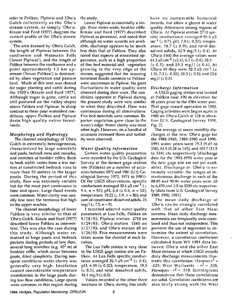
refer to Palikea, Pipiwai and 'Ohe'o Gulch collectively as the 'Ohe'o stream system, or simply 'Ohe'o. Kinzie and Ford (1977) diagram the vertical profile of the 'Ohc'o strcam system.
The area drained by 'Ohe'o Gulch, the length of Pipiwai between the confluence and Waimoku Falls ('lower Pipiwai'), and the length of Palikea between the conflirence and a point approximately 1.5 km up- stream ('lower Palikea') is dominat- ed by alien vegetation and pasture land. Much of this area was cleared for sugar planting and cattle during the 1920's (Kinzie and Ford 1977). Although sugar is gone, cattle are still pastured on the valley slopes above Palikea and Pipiwai. In sharp contrast to these poor watershed con- ditions, upper Palikca and Pipiwai drain high quality native forest- lands.
M o r p h o l o g y a n d H y d r o l o g y The channel morphology of 'Ohe'o
Gulch is extremely heterogeneous, characterized by large waterfalls and pools, bedrock runs and cascades, and stretches of boulder riffles. Bank to bank width varies from a iew me- ters at constricted bedrock runs to more than 50 meters in the larger pools. During the period of this study, flow was extremely variable but for the most part continuous in time and space. Large flood events were common. Water clarity was usu- ally low near the terminus but high in the upper reaches.
The channel morphology of lower Palikea is very similar to that of 'Ohe'o Gulch. Kinzie and Ford (1977) described lower Palikea as intermit- tent, This was also the case during this s tudy . Although water re- mained in large pools and bedrock pockets during periods of low flow, several long stretches (e.g. lo2 m) of boulder riffle, which occur between pools, dried completely. During non- spate conditions water clarity was generally very high. Insolation caused considerable temperature stratification in the large pools dur- ing low flow conditions. Large spates were common in this region during
the study. Lower Pipiwai is essentially a sin-
gle, three meter-wide, boulder riffle. Kinzie and Ford (1977) described Pipiwai as perennial, and noted that although no water records arc avai'l- able, discharge appears to be much less than that of Palikea. They also noted that aspects of streambed ap- pearance, such as a high proportion of fine bed material and vegetation growing to the very edge of the strcam, suggested that the 'scouring torrential floods common to Palikea' were uncommon in Pipiwai. No great fluctuations in water quality were observed during their work. The con- ditions apparent at Pipiwai during the present study were very similar to what they described. Flow was continuous during all observations. Fine bed materials wcre common. Ri- parian vegetation grew close to the water's edge. Water clarity was most often high. However, on a handful of occasions increased flows and turbid- ity were observed.
W a t e r Q u a l i t y Informat ion Certain water quality parameters
wcre recorded by the U.S. Geological Survey at the former gage station site (Palikea) on a number of occa- sions between 1972 and 1981 (U.S. Ge- ological Survey 1972, 1974 to 1981). Of the USGS observations, specific conductance averagcd 33.6 )rS cm-I (i 9.4, n = 52); pH, 6.8 ( i 0.4, n = 52); temperature, 19.22 ( i 1.9, n = 50); and sum of constituent dissolved solids, 23 mg/l (i 7.5, n = 9).
I recorded selected water quality parameters at Lua Falls, Palikea on 5/28/93; Pipiwai station 2710 on 5/29/93; 'Ohe'o station 1560 on 5/27/93; and 'Ohe'o station 40 on 5/26/93. Five measurements were taken across the channel at each lo- cation.
The Lua Falls station is very close to the USGS gage station site on Pa- likca. At Lua Falls specific conduc- tance averaged 32.3 $ 3 cm-I (k 0.4); pH, 6.59 ( 2 0.32); temperature, 19.5 (k 0.3); and total dissolved solids, 16.1 mg/l (k 0.3).
Values recorded at the other three locations in 'Ohe'o during this study
have no comparable historical records, but ailow a glance at water quality diffcrenccs among regions of 'Ohc'o. A t Pipiwai station 2710 spc- cific conductance avcragcd 85.5 pS an-' (1 0.7); pi 1, 7.0 (1 0.32); tcmper- ature, 18.7 (+ 0.9); and total dis- solved solids, 42.9 mg/l (+ 0.4). At 'Ohc'o 1560 the average values were 61.2 pS cm-I (~2.4) ; 6.7 (L 0.4); 20.3 (k 0.3); and 29.1 m g / l (+ 0.4). At 'Ohc'o 40 they were 52.3 jtS cm-I (k 1.3); 7.3 (k 0.32); 20.3 (k 0.3); and 23.6 mg/l (i 0.3).
Discharge In format ion A USGS gaging station was located
at Palikca near 490 m elevation for 48 years prior to the 1984 water year. That gagc ceased operation in 1983. Gaging activities were begun again in 1988 on 'Ohe'o Gulch at 128 m elcva- tion (U.S. Geological Survey 1991, Fig. 2).
The average of mean monthly dis- charges at the new 'Ohe'o gagc for the 1988-1989, 1989-1990 and 1990- 1991 water years were 79.3 (9.65 to 218), 61.5 (5.28 to 145), and 101.7 (12.5 to 334) cfs respectively (discharge data for the 1992-1993 water year at the new gage site are not yet avail- able). Discharge in 'Ohe'o is ex- tremely variable: the ranges of in- stantaneous discharge in each of the 88-89 and 90-91 water years wcrc -63 to 6,470 and 2.5 to 3200 cfs rcspective- ly (data from US. Geological Survey 1989, 1990,1991).
The mean daily discharge of 'Ohe'o can be strongly correlated with that of other East Maui streams. Mean daily discharge mea- surements are temporally auto-corre- lated and thus not independent. This prevents the use of regression to de- termine the extent of correlation. However, a correlation coefficient calculated from WY 1991 data be- tween 'Ohe'o and the other East Maui streams at which USGS records daily discharge measurements illus- trates this correlation: I lanawi-r2 = ,623; West Wailuaiki - r2 = .535; IIonopou - r2 = .518. Scattergrams demonstrate that these correlations are solid. Correlation coefficients are also fairly s t rong with the West
1994. Hodges. Population Monitoring. CPSUAJH. 2
Maui stream 'Iao - r2= .542. Gaged streams further west than Iao exhib- it a positive correlation but scatter- grams indicate curvilinearity and in- creasing variability in the residuals with increasing discharge.
METHODOLOGY
Sta t ion Layout
trapping was used to survey M. iar.
Direct O b s e r v a t i o n I used direct observation to survey
the populations of hihiwai, 'o'opu, and 'iipac. Observations were madc in randomly placed quadrats. Obser- vations at each quadrat were re- stricted to a specific period of time for each of '6pae and 'o'opu.
Ten quadrats were used at each sta- tion to survey hihiwai, 'o'opu, and '6pae. Quadrats locations were dif- ferent for each taxa, but fixed for a given taxa throughout the study.
tilt crrca; Thc sampling area (the arcn from which samples were drawn) at each station was fixed. This prevented variation in sam- pling fraction among stations, and
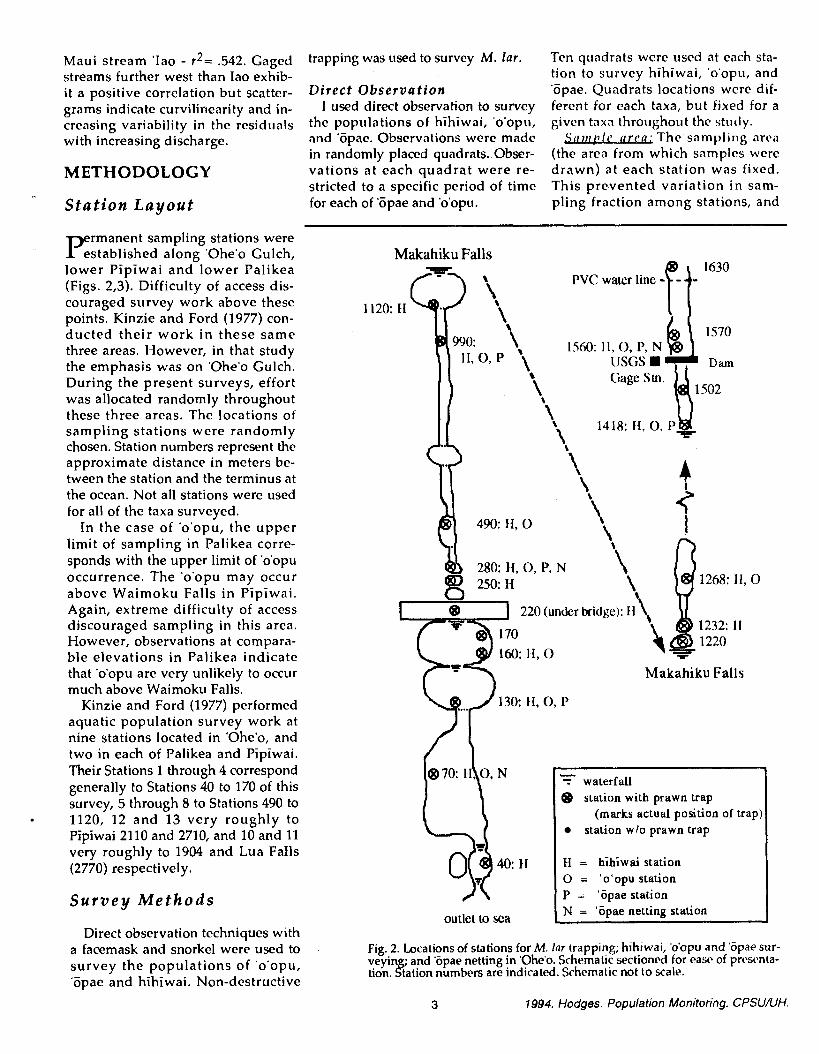
I? rmanent sampling stations were established along 'Ohe'o Gulch,
lower Pipiwai and lower Palikea (Figs. 2,3). Difficulty of access dis- couraged survey work above these points. Kinzie and Ford (1977) con- ducted their work in these same three areas. However, in that study the emphasis was on 'Ohe'o Gulch. During the present surveys, effort was allocated randomly throughout these three areas. The locations of sampling stations were randomly chosen. Station numbers represent thc approximate distance in meters bc- tween the station and the terminus at the ocean. Not all stations were used for all of the taxa surveyed.
In the case of 'o'opu, the upper limit of sampling in Palikea corre- sponds with the upper limit of 'o'opu occurrence. The 'o'opu may occur above Waimoku Falls in Pipiwai. Again, extreme difficulty of access discouraged sampling in this area. However, observations at compara- ble elevations in Palikea indicate that 'o'opu are very unlikely to occur much above Waimoku Falls.
Kinzie and Ford (1977) performed aquatic population survey work at nine stations located in 'Ohe'o, and two in each of Palikea and Pipiwai. Their Stations 1 through 4 correspond generally to Stations 40 to 170 of this survey, 5 through 8 to Stations 490 to 1120, 12 and 13 very roughly to Pipiwai 2110 and 2710, and 10 and 11 very roughly to 1904 and Lua Falls (2770) respectively.
S u r v e y M e t h o d s
Direct observation techniques with a facemask and snorkel were used to survey the populations of 'o'opu, '6pae and hihiwai. Non-destructive
- - waterfall station with prawn trap
(marks actual position of trap) station wlo prawn trap
H = hihiwai station 0 = 'o'opu station P = 'Gpae station N = 'Gpae netting station outlet to sea
Fig. 2. Locations of stations for M. Inr trapping; hihiwai, 'o'opu and 'opae sur- veyin ; and 'opae netting in 'Ohe'o. Schematic sectioned for ease of prcwnta- tion. h i o n numbers are indicated. Schematic not to scale.
3 1994. Hodges. Population Monitoring. CPSUNH.

'Lua Falls'
(2770): P, N
W aimoku Falls
Palikea Falls
Fig. 3. Locations of stations for M. lar tra ing; h~h~wai, 'o'opu and 'o ac sur- veying; and 6pae netting in Palikea and Ttpwai. Schematic sectionex [or rasp of presentation. Station numbers are indicated. Schchmatic not to scale. See Fig. 2 for legend.
hence prevented area-based varia- tion in sampling intensity. The sam- pling area a t each station was de- fined as one hundred square meters for h ihiwai , a n d t h r e e h u n d r e d square meters for 'o'opu and '6pae.
Bank to bank width was measured to the nearest meter a t the time of initial establishment of each sta- tion. The lengths (upstream-down- stream dimension) of stream to be sampled at each station for hihiwai and 'o'opu/'opae were determined by dividing one hundred and three hun- dred square meters respectively by the bank to bank width. For exam- ple, the approximate bank to bank width at the station shown in Figure 4 is four meters. Hence, the length of the area from which samples will be drawn at this station for hihiwai is 10014 = 25 meters, for 'o'opul'opae 30014 = 75 meters. Thus the dimen-
sions of the sampling areas at this station are 25x4 (hihiwai) and 75x4 ('o'opu 1'6pae).
Coord ina te s v s t e m : A frequently shifting substrate discourages the use of permanent quadrat markers in most Ilawaiian streams. I Ience, the quadrat locations were defined as Cartesian coordinates (Fig. 4 - see Appendix 1 for coordinates used). Once the dimensions of the sampling areas at a given station were detcr- mined, the coordinates to be used for quadrat placement a t that station were found by randomly choosing pairs of numbers falling within the respective dimensions of the sample areas.
During survey work, the observer began at the station benchmark, de- fined as (0,O). Although the bench- mark can be any permanent object, the station flag was used throughout
this survey. The observer paced off the necessary number of meters up the stream from the benchmark, then paced off the necessary number of me- ters from the right bank to relocate the correct area for placement of the first quadrat . Once observation in that quadrat was completed the pro- cess was repeated, using the current - quadrat location as the point of de- parture, to find the location of the next quadrat.
If, d u r i n g placement of the quadrat, an observer encountered an object such as a log or largc rock which protruded above water level and which obstructed > ca. 40% of the quadrat, the quadrat was moved directly upstream. Quadrats contain- ing less dry surface area than this were not moved.
It was not possible to survey the bottom of deep pools. Instead, the co- ordinate system was modified to place the quadrats around the pool periphery (Fig. 5). SCUBA should be employed in the future to determine faunal occurencc in deep pools, and the correlation between faunal densi- ties in mid-pool and those on the pe- riphery.
'o'opu: The density and size class distribution of all species of 'o'opu (alamo'o, nopili, and n i k e a have been observed to date) were recorded using ten 1m2 quadrats at each of 18 stations. After carefully approach- ing the proper quadrat location via the coordinate system, the observer used a one meter long, narrow wire rod to quickly determine and visual- ize the four corners of the lm2 quadrat. The observer watched the defined area for th ree minutes, recording thc highest number of each size class of each species occurring within the quadrat. Inches were used as thc unit of measurement because I felt less comfortable with the metric equivalent during visual estimation. Individual 'o'opu less than 0.5 in. standard length were classified as h inana, r egard less of species. (Naked eye determination of species at this size is not feasible). Other size classes were defined using half inch increments between 0.5 and 9 inches. Any individual over nine
1994. Hodges. Population Monitoring. CPSUAJH. 4

inches in standard length was placed in a single 9 I class.
Aftcr thc obscrvalion period al each quadrat the observer classificd the habitat, the substrate composi- tion wi thin the quadra t , a n d the depth in centimeters at the center of the q u a d r a t . Hab i ta t types uscd were riffle ( > 30 cm depth, primari- ly cobble/ gravel substrate), boulder r iff le (var iable dep th , pr imari ly rock and boulder substrate), pool, run (variable depth, significant current, primarily bedrock substrate), and edgewater (edge of channel, shal- low, little to no current, often high si l t a n d vegeta t ion, noticeably higher water temperature than mid- channel).
Substrate composition was dcsig- nated as perccnt cover of sand (< 5 mm longest diamcter), gravel (5 5 x < 20), cobbles (20mm s x < 15 cm), rocks (15 cm s x 40 an), boulders ( 2 4-0 cm), and bedrock. Detritus, though fairly rare, occurred in a layer above the substrate. Percent detrital cover was recorded separately.
All observations were made by my- self and Anne Brasher. Working to- gether, w e each counted five quadrats at each station. One observ- e r counted the five seaward-most quadrats, while the other counted the five quadrats above these. It was both safer and a lesser disturbance to the ' o 'opu if t h e observer ap- proached the quadrat from down- stream. Consequently, observers al- ways began with the downstream- most quadrat in a set of five, and worked upstream. After each observ- e r had counted the assigned set of five quadrats both observers moved on to the next station.Though each observer always counted half of the quadrats a t each station the given half counted was not necessarily the same during all surveys.
Stations were not counted in any particular order. However, we com- monly worked through a given reach by starting with the seaward-most station in the reach and working up- wards. It took three days to count all of the 'o'opu stations.
' 6 p a e : Trapping vs. Direct Obser- vation: On a number of occasions
sampling area -25 meters
long for hihiwai -75 meters
long for 'o'opu and 'opae
sampling area approx. -
4 meters wide
upstream
Station flag = (0,O)
Fig. 4. Use of Cartesian coordinate system to define quadrat locations in stream channel. Dimensions of sampling awa indicatcd. Quadrats shown are 1 m2.
outlet outlet
A: Count sample area 'length' B: Count sunlple area 'wdth ' in clockwise direction along perimeter towards center ofpool. of pool.
Fig. 5. Adaption of cartesian coordinate system to deep pools.
'Zipae were found in the prawn traps during preliminary prawn trapping efforts. Trapping has clear advan- tages over dircct obscrvation in terms of sampling cffort, accuracy of count and size frequency distribution, op- portunity to determine sex ratio and perccnt fecundity, presence of dis- ease /parasites, etc. The 'ijpae feed primarily on filamentous algae and detritus (Couret 1976). However, the occurrence of individuals in the M. 1 a r traps suggested that '6pae might be trapped with the same bait used for M. l a r . O r '6pae might enter a trap while moving about.
To determine if 'ijpae might be eas- ily trapped, 1 constructed three small traps following thc design and bait- ing scheme of those for M. lar (mesh size = 118 in2, d iameter = 8 in., length = 12 in.) . Traps were left
overnight on 1 / 20 193 in an area with abundant '6pae ncar Station 2170. No 5 p a c were caught. Consrqucntly, I chose to survey 'iipae abundance by using a modification of the direct ob- servat ion method developed for 'o'opu.
Night vs. Day Counts: Nishimoto (1992), using a visual survey method, observed a higher abundance of '6pae during the late evening hours than during the day at three locations in Hakalau Stream on Hawai'i. In ad- dition, dur ing the day Nishimoto saw 'iipae primarily along the edge of the channel. But, during the late evening hours Nishirnoto saw 'Gpae occur throughout the channel.
Population survcys conducted for monitoring and among-stream com- parisons nccd only to provide a con- sistent indcx of abundance, regardless
5 1994. Hodges. Population Monitoring. CPSUAJH.
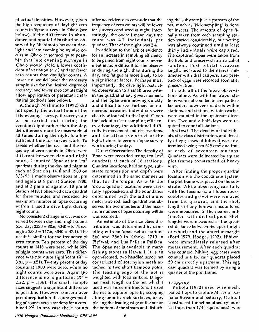
of actual densities. However, given the high frequency of daylight zcro counts in 'Zipae surveys in 'Ohe'o (see below), if the difference in abun- dance and spatial distribution ob- served by Nishimoto between day- light and late evening hours also oc- curs in 'Ohe'o, it seemed quite possi- ble that late evening surveys in 'Ohe'o would yield a lower coeffi- cient of variation (c.v.) and/or fewer zero counts than daylight counts. A lower C.V. would lower the necessary sample size for the desired degree of accuracy, and fewer zero counts might allow application of parametric sta- tistical methods (see below).
Although Nishimoto (1992) did not specify the actual time of the 'late evening' survey, if surveys are to be carried out during the eveninglnight rather than the day, the difference must be observable at all times during the night to allow sufficient time for survey work. To assess whether the C.V. and the fre- quency of zero counts in 'Ohe'o were different between day and night hours, I counted 'iipae at ten l m 2 quadrats during the day and night at each of Stations 1418 and 1900 on 3/3/93. I made observations at lpm and again at 9 pm at Station 1900, and at 2 pm and again at 10 pm at Station 1418. I observed each quadrat for three minutes, and recorded the maximum number of 'iipae occurring within. I used a dive light during night counts.
No consistent change in c.v. was ob- served between day and night counts (c.v. day: 2330 = 80.6, 3040 = 85.5; C.V. night: 2330 = 117.6, 3040 = 47.1). The result is similar for the frequency of zero counts. Ten percent of the day counts at 1418 were zero, while 50% of night counts were zero. This differ- ence was not quite significant (x2 = 3.81, p = .051). Twenty percent of day counts at 1900 were zero, while no night counts were zero. Again the difference is not significant (x* = 2.22, p = .136). The small sample sizes suggests a significant difference is possible. However, concern over pseudoreplication discourages pool- ing of counts across stations for a com- bined x2 . In any case these counts
offer no evidcnce to conclude that the frequency of zcro counts will bc lower for surveys conducted at night. Intcr- cstingly, the overall mean daytime count was 4.7 individuals pcr quadrat. That of the night was 2.4.
In addition to the lack of evidcnce for an increase in sampling efficiency to be gained from night counts, move- ment is more difficult for the observ- er during the night than during the day, and fatigue is more likely to be a significant factor. Perhaps most importantly, the dive light restrict- ed observation to a small area with- in the quadrat at any given moment, and the 5pae were moving quickly and difficult to see. Further, on nu- merous occasions individuals were clearly attracted to the light. Given the lack of a clear sampling efficien- cy advantage, the additional diffi- culty in movement and observations, and the attractive effect of the light, I chose to perform 5pae survey work during the day.
Direct Observation: The density of 'iipae were recorded using ten lm2 quadrats at each of 16 stations. Quadrat locations, habitat type, sub- strate composition and depth wcrc determined in the same manner as that for the 'o'opu. As with the 'o'opu, quadrat locations were care- fully approached and the boundaries determined with the aid of a one meter wire rod. Each quadrat was ob- served for two minutes and the maxi- mum number of 5pae occurring within was recorded.
An estimate of the size class dis- tribution was determined by sam- pling with an '6pae net at stations 560 and 2560 in 'Ohe'o, 2710 in Pipiwai, and Lua Falls in Palikea. The 'Zipae net is available in many fishing stores in IIawai'i. It is an open-fronted, two handled scoop net constructed of soft nylon mesh at- tached to two short bamboo poles. The leading edge of the net is weighted with lead sinkers. Diago- nal mesh length on the net which I used was three millimeters. I used the net to capture 'iipae by scooping along smooth rock surfaces, or by placing the leading edge of the net on the bottom of the stream and disturb-
ing the substrate just upstream of the net, much as 'kick-sampling' is done for insects. The amount of 5pae fi- nally taken from each sampling sta- tion varicd considerably, but netting was always continued until at least thirty individuals were captured. The captured 'Zipae were taken from the field and prcscrvcd in an alcohol solution. Post orbital carapace length, measured to the nearest mil- limeter with dial calipers, and pres- ence of eggs were recorded soon after prcserva tion.
I madc all of the '6pac observa- tions alone. As with the 'o'opu, sta- tions were not counted in any particu- lar order, howcvcr quadrats within stations, and stations within reaches wcrc counted in the upstream direc- tion. Two and a half days were re- quired to count all stations.
h ih iwa i : The density of individu- als, size class distribution, and densi- ty of egg cases of hihiwai were de- termined using ten 625 cm2 quadrats at each of scventcen stations. Q~ladrats were delineated by square plot frames constructed of heavy wire.
Aftcr finding the proper q ~ ~ a d r a t location via the coordinate system, the plot frame was placed on the sub- strate. While observing carefully with the facemask, all loose rocks, cobbles and gravel were removed from the quadrat , and the shell lengths of any hihiwai encountered wcre measured to the nearest mil- limeter with dial calipers. Shell lengths wcre measured as the great- est distance between the apex (origin of whorl) and the anterior margin (Ford 1979, Hodges 1992). Hihiwai wcre immediately released after mcasurcment. After each quadrat was counted, hihiwai egg cases were counted in a 156 cm2 quadrat placed 50 cm directly upstream. This egg case quadrat was formed by using a quarter of the plot frame.
T r a p p i n g Kubota (1972) used wire mesh,
baited traps to capture M. lnr in Ka- hana Stream and Estuary, O'ahu. I constructed funnel-mouthed cylindri- cal traps from 114" square mesh wire
1994. Hodges. Population Monitoring. CPSUAJH. 6

hardware cloth (Fig. 6). I designed the traps to be particularly large to reduce 'trap saturation' by high den- sities of M. lar. Each trap was baited by placing 35 pieces of dry commcr- cia1 dog food in the bait box (Purina Dog Chow@ was used throughout). Wire was used to suspend and fasten the bait box inside and near the back of the trap.
Twenty eight trapping stations were established throughout 'Ohe'o, Pipiwai and Palikea (Figs. 2,3). A single trap was placed at each of these stations. The actual location of a trap at a given station (e.g. riffle vs. pool) may significantly affect the catch at that station. Hence, Figs. 2,3 indicate the relative trap location at each station.
A full trapping survey was a three day process requiring the efforts of at least two people. One t rap was placed at each of fourteen stations during the afternoon of the first day. Traps were fully submerged during placement, with the mouth facing downstream to avoid collection of floating debris. Traps were secured to the stream bank with rope. Traps were retrieved the next morning in the order that they were placed. Re- trieval of this first set of fourteen traps was completed by noon. The next set of fourteen traps were placed at those stations which were not trapped the previous night. These traps were retrieved during the morning of the third day, again in
the order that they werc placed. Data was obtained from the catch
immediately after each trap was re- trieved, and prawns were subscquent- ly released. Post orbital carapace length was measured to the nearest millimeter. Presence of eggs was also recorded. Sex was determined accord- ing to the methods of Kubota (1972). Only those individuals r 12 mm carapace length were sexed. Individ- uals smaller than this were difficult to sex under field conditions. Record- ing of sex data was begun in March.
Kubota (1972) reported the occur- rence of large carapace lesions in M. 1 a r in Kahana Estuary on O'ahu. l i e attributed the lesions to fungal infec- tion and termed the symptoms "black-spotted disease." The occur- rence of large lesions and deforma- tions of the carapace in M. l a r in 'Ohe'o was noticed during the March trapping. The lesions, which were often severe enough to fully expose many of the internal organs, closely matched Kubota's photograph and description of "black-spotted dis- ease." 1 began systematic recording of the incidence of symptoms during the third trapping. Symptoms (lesions and/or deformations) were scored on a presence /absence basis.
Pua 'a lu 'u Stream Limited survey work was carried
out in Pua'alu'u Stream. Pua'alu'u is a small, second-order stream occur- ring just to the north of 'Ohe'o. The
watershed is 63 ha, in area, head- waters occur at ca. 600 m elevation, channcl length is 2.4 km, and dis- charge has been reported as .27 cfs (Kinzie & Ford 1979). The segment of Pua'alu'u between the H5na High- way and the terminus is steep. Flow movcs through a number ot small plunge pools and over bedrock cas- cades and steep runs. Flow is deposit- ed dircctly onto the beach through a stccp, narrow chute. The macrofauna populations of Pua'alu'u were sur- veyed by Kinzie and Ford (1979). They provide photographs and a de- scription of the stream and water- shed.
During the year in which this study was conducted, the water in Pua'alu'u was characteristically clear. Pua'alu'u is considered by local residents to be largely spring-fed, and is apparently a primary source of drinking water because of its high quality. On 12/4/93, the five streams from 'Ohe'o to Wailua, except Pua'altc'u, wcre spating or showing obvious signs of increased flow and turbidity. Pua'alu'u was at normal flow level and the water was clear. This suggests that the flow regime of Pua'alu'u is independent of the other streams in the vicinity. Independence might be caused by some combination of small watershed size, elevation of headwaters, or a preponderance of spring water rather than runoff.
I surveyed Pua'alu'u at three sta- tions which roughly correspond to Stations 70, 130; and 280 in 'Ohe'o (see Appendix 11 for quadrat coordi-
rope to secure nates used in Pua'alu'u). The initial trap to bank survey was carried out on 713-4193.
10 cm diam. The purposc of the initial survey was . -
to compare the fauna of lbwer
T Pua'alu'u with lower 'Ohe'o. 1 Iow- ever, on numerous occasions high flow prevented 'o'opu survey work in
46 cm diam.
1 'Ohe'o. I uscd some of these opportu-
bait box suspended nities to carry out additional surveys with wire inside trap of Pua'alu'u: Two back-to-back sur- - veys were carried out on 10 15-6/93
97 cm and 1016-7/93. These surveys were
stream flow direction intended to provide a rough assess- ment of the error rate of the counting method under a limited sampling
Fig. 6. Diagram of wire mesh trap used for M. lor. scenario. A follow-up survey was performed on 12/4/93. The 1214 sur-
7 1994. Hodges. Population Monitoring. CPSUAJH.
vey was the first to incorporate new personnel beyond myself and A. Brasher, and I considered this survey partly a training exercise.
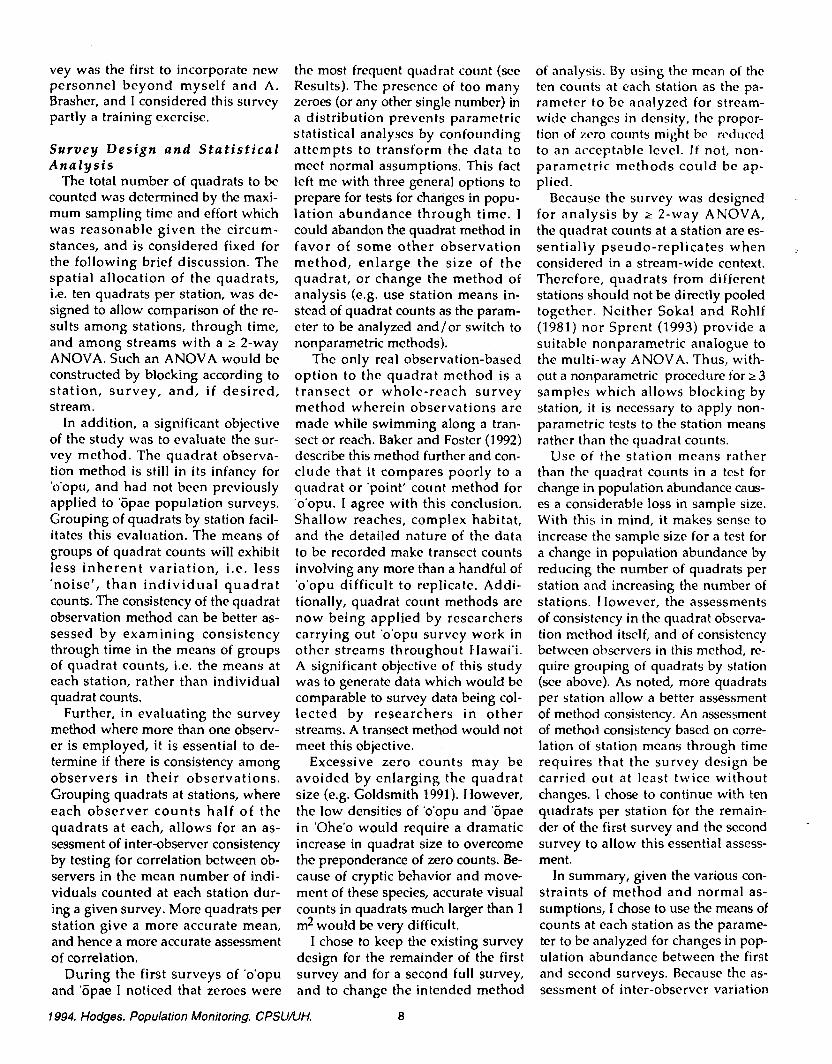
Survey Des ign and S t a t i s t i c a l A n a l y s i s
The total number of quadrats to be counted was determined by the maxi- mum sampling time and effort which was reasonable given the circum- stances, and is considered fixed for the following brief discussion. The spatial allocation of the quadrats, i.e. ten quadrats per station, was de- signed to allow comparison of the re- sults among stations, through time, and among streams with a 2 2-way ANOVA. Such an ANOVA would be constructed by blocking according to stat ion, survey, and, if des i red, stream.
In addition, a significant objective of the study was to evaluate the sur- vey method. The quadrat observa- tion method is still in its infancy for 'o'opu, and had not been previously applied to 'Zipae population surveys. Grouping of quadrats by station facil- itates this evaluation. The means of groups of quadrat counts will exhibit less i n h e r e n t var ia t ion, i.e. less 'noise', than ind iv idua l q u a d r a t counts. The consistency of the quadrat observation method can be better as- sessed by examining consistency through time in the means of groups of quadrat counts, i.e. the mcans at each station, rather than individual quadrat counts.
Further, in evaluating the survey method where more than one observ- er is employed, it is essential to de- termine if there is consistency among observers in thei r observations. Grouping quadrats at stations, where each observer coun ts half of the quadrats a t each, allows for an as- sessment of inter-observer consistency by testing for correlation between ob- servers in the mean number of indi- viduals counted at each station dur- ing a given survey. More quadrats per station give a more accurate mean, and hence a more accurate assessment of correlation.
During the first surveys of 'o'opu and '6pae I noticed that zeroes were
the most frequent quadrat count (see Results). The prescncc of too many zeroes (or any other single number) in a distribution prevents paramctric statistical analyses by confounding attempts to transform the data to meet normal assumptions. This fact left me with three general options to prepare for tests for changes in popu- lation abundance through time. 1 could abandon the quadrat mcthod in favor of some other observation method , enlarge the s ize of t h e quadrat , or change the method of analysis (e.g. use station means in- stead of quadrat counts as the param- eter to be analyzed and/or switch to nonparametric methods).
The only real observation-based option to the quadrat method is a transect o r whole-reach survey method wherein observations are made while swimming along a tran- sect or reach. Baker and Foster (1992) describe this method further and con- clude that it compares poorly to a quadrat or 'point' count method for 'o'opu. I agree with this conclusion. Shallow reaches, complex habitat, and the detailed nature of the data to be recorded make transect counts involving any more than a handful of 'o'opu difficult to replicate. Addi- tionally, quadrat count methods are now being applied by researchers carrying out 'o'opu survey work in other streams throughout I Iawai'i. A significant objective of this study was to generate data which would be comparable to survey data being col- lected by researchers in o ther streams. A transect method would not meet this objective.
Excessive zero counts may be avoided by enlarging the quadrat size (e.g. Goldsmith 1991). However, the low densities of 'o'opu and 'iipae in 'Ohe'o would require a dramatic increase in quadrat size to overcome the preponderance of zero counts. Be- cause of cryptic behavior and move- ment of these species, accurate visual counts in quadrats much larger than 1 m2 would be very difficult.
I chose to keep the existing survey design for the remainder of the first survey and for a second full survey, and to change the intended method
of analysis. By using thc mcan of the ten counts at each station as the pa- rameter to be analyzed for stream- wide changes in density, the propor- tion of zero counts might bc rccluwd to an acceptable level. I f not, non- parametric methods could be ap- plied.
Because the survey was designed for analysis by r 2-way A N O V A , the quadrat counts at a station are es- sentially pseudo-replicates when .. considered in a stream-wide context. Therefore, quadrats from different stations should not be directly pooled together. Neither Sokal and Rohlf (1981) nor Sprent (1993) provide a suitable nonparametric analogue to the multi-way ANOVA. Thus, with- out a nonparametric procedure for r 3 samples which allows blocking by station, i t is necessary to apply non- parametric tests to the station means rather than the quadrat counts.
Use of the station means rather than the quadrat counts in a test for change in population abundance caus- es a considerable loss in sample size. With this in mind, it makes sense to increase the sample size for a test for a change in population abundance by reducing the number of quadrats per station and increasing the number of stations. 1 Iowever, the assessments of consistency in the quadrat observa- tion method itself, and of consistency between observers in this method, re- quire grouping of quadrats by station (see above). As noted, more quadrats per station allow a better assessment of method consistency. An assessment of method consistency based on corre- lation of station means through time requires that the survey design be carried out at least twice without changes. I chose to continue with ten quadrats per station for the remain- der of the first survey and the second survey to allow this essential assess- ment.
In summary, given the various con- straints of method and normal as- sumptions, I chose to use the means of counts at each station as the parame- ter to be analyzed for changes in pop- ulation abundance between the first and second surveys. Because the as- sessment of inter-observer variation
1994. Hodges. Population Monitoring. CPSU/UH. 8

and overall method consistency re- quire a fairly large number of quadrats per station, and an un- changed design through at least two surveys, I chose to remain with ten quadrats per station for the comple- tion of the first, and the second sur- vey.
Once the method is found to be son- sistent, it is appropriate to change the survey design to increase the sta- tistical power and sampling efficien- cy of future surveys. Using the data from the first and second 'iipae and 'o'opu surveys I evaluate changes in the survey design in terms of statisti- cal power (see Discussion).
Both t h e Kruska l -Wal l i s a n d Friedman tests detect differences in locations or means among 23 samples. of these, only the Kruskal-Wallis tolerates differences in sample size and is used here. The multiple com- parison proccdure used with the Kruskal-Wallis test is from Sprent (1993). All results reported from rank-based nonparametric tests are corrected for ties.
RESULTS
urveys in 'Ohe'o were begun in S e a r l y January, 1993. The 'o'opu were counted on 2 /5-7/93 and 5 14- 6 193. The '5pae were counted and net- ted on 313-5193 and 5126-29193. Heavy ra infa l l and turbidi ty re- peatedly prevented the additional 'o'opu and 'iipae surveys which were scheduled. Hihiwai were surveyed on 1 / 19-21 193, 3 1 20-21 1 93, and 5 / 26- 29/93. Prawns were trapped on 113- 5/93,3/31-4/2/93, 7117-19/93, and 11 120-23193.
The ' o ' o p u in ' O h e ' o
Figure 7 illustrates the frequency distributions of quadrat counts from the first and second surveys.
Temporal Differences Comparisons Between Surveys 1 and 2 of Densities of Enfire Populations
All species - all sizes: The mean number of 'o'opu of all species at each station during the 215-7193 survey
ranged from 0 to 3.1 'o'opu per quadrat , and thc mcan of these means was .619 (n = 16, variance = .783). The mean number of all species of 'o'opu at each station during the 514-6193 survey ranged from 0 to 2.3 'o'opu per quadrat, and the mean of thcsc means was .567 (n = 18, vari- ance = .471). The station mcans of the raw counts from each of the first and second surveys are randomly dis- tributed (Elliott's (1971) Index of Dispersion: irst: X* = 22.6, d. f. = 17; second: X Z f = 14.1, d. f . = 17). A d(x+.05) transformation normalized the station means of the first and sec- ond surveys (Lilliefors test for de- parture from normality- First survey: n = 16, all comparisons c .213, p > .05. Second survey: n = 18, all compar- isons < ,200, p > .05 (Sprcnt 1993, p. 79). The difference in the means of station means was not significant (mcan xi - yi = -.0006, d . f . = 15, paired t = -.102, p > SO). Iiowever, the test has very low power to detect the observed 9.2% change in the mean of station means (see Discus- sion).
alamo'o - all sizes: The mean num- ber of 'alamo'o at each station during the 215-7193 survey ranged from 0 to 2.1 individuals per quadrat, and the mean of these means was .437 (n = 16, variance = ,472). The mean number of 'alamo'o at each station during the 5/4-6193 survey ranged from 0 to 1.5 individuals per quadrat , and the
mean of thcsc mcans was ,361 (n = 18, variance = .213). A paircd-t tcst has very low power to detect the ob- served 21% change in the mcan of station mcnns (scc Discussion).
n5kea - all sizes: Thc mean number of nakea at each station during the 215-7193 survey ranged from 0 to .3 individuals per quadrat , and the mean of these mcans was .05 (n = 16, variancc = .012). The mean number of nakea at each station during the 514- 6/93 survey ranged from 0 to 1.9 indi- viduals per quadrat, and the mean of these means was .I67 (n = 18, vari- ance = .2). Although the observed 334% change in the mean of station means would be detected by the paired t tcst, the data cannot be nor- malized. Using the nonparamctric two-sample analogue, this difference in the mcan of means was not signifi- cant (Mann-Whitney U = 123, Z = - .936, p > .30).
nopili - all sizes: No nopili were recorded at any of the 16 stations ob- served during the 2/5-7193 survey. The mean number of nopili at each station during the 514-6193 survey ranged from 0 to .2 individuals per quadrat , a n d the mean of these means was .011 (n = 18, variance = .002). The data cannot be normalized. Using the nonparametric two-sam- ple analogue, this difference in the mean of means was not significant (Mann-Whitney U = 136, Z = -.943, p > .30).
hinana - all sizes: Thc mean num-
Total number of 'o'opu per quadrat
Fig. 7. Frequency distribution of the number of 'o'opu per quadrat ('alamo'o, nopili, nakea and hinana combintd, all quadrats at all stations combined) rtcordrd in the 'Ohe'o Stream System during thv first and second surveys.
9 1994. Hodges. Population Monitoring. CPSUNH.

ber of hinana at each station during the 2 15-7/93 survey ranged from 0 to 1.2 individuals per quadrat, and the mean of these means was .I31 (n = 16, variance = .113). The mean number of hinana a t each station during the 5/46/93 survey ranged from 0 to .3 individuals per quadrat, and the mean of these means was .028 (n = 18, variance = .007). The observed 467% change in the mean of station means would be detected by the paired t test. However, the data cannot be normalized. Using the nonparametric two-sample analogue, this difference in the mean of means was not signifi- cant (Mann-Whitney U = 131.5, Z = - .7, p > -40).
Comparisons Between Surveys 1 and 2 of Spatial Distribution of Densities of Entire Populations
All species - all sizes: The mean number of 'o'opu of all species, in- cluding hinana recorded at each sta- tion during the first survey was highly correlated with that at each station during the second survey
(Kendall 's t a u = .711, n = 16, Z = 3.839, p c .0005).
'alamo'o - all sizes: Thc same was true for the mean number of 'alamo'o at each station (Fig.8; (Kendall's tau = .587,n= 16, Z =3.173,p < .005). Fig- ure 8 also illustrates the high densi- ties observed in the lowest and upper reaches.
niikea - all sizes: A similar pattern is visible for the mean number of n5kea (Fig. 8; Kendall's tau = .%4, n = 16, Z = 5.209, p <c .0001), however a look at the undue influence of zero counts and considerable non-linearity visible in a scattergram cautions against strong conclusions for this species. In any case, the restriction of this species to the lower and mid reaches of the 'Ohe'o Stream System is clear from Figure 8.
nopili - all sizes & hinana: Nei- ther the number of niipili nor the number of hinana observed were suf- ficient to make this a meaningful comparison.
- . - - . - . - 6 i t o o 2600 - 3 060
distance inland (m)
Fig. 8. Mean number of 'o'opu recorded at each station during the first and sec- ond surveys, 'Ohe'o Stream System.
Comparisons Between Surveys 2 and 2 of Size-Frequencies of Entire Popu- la t ions
All species (w / o hinana): The ob- served difference in frequency distri- bution between the first and second surveys was not significant (X2 = 8.098, d . f . = 5, p = .1509; size classes r "3 to 3.5" pooled for each survey to satisfy minimum sample require- mcnts of counts 2 one for each catego- ry - e.g. Koopmans 1987, p. 420).
alamo'o: Figure 9 illustrates the size frequency distribution of 'alamo'o observed throughout the 'Ohe'o Stream System during the first and second surveys. The ob- served difference in frequency distri- bution between the first and second surveys was not significant (x* = 5.138, d .f. = 4, p = .2735; size classes ;?
"2.5 to 3" pooled for reasons above). niikea: Figure 9 illustrates the size
frequency distribution of niikea ob- served throughout the 'Ohe'o Stream System during the first and second surveys. The observed difference in frequency distribution between the first and second surveys was not sig- nificant (x* = 2.305, d . f. = 4, p = .6798; size classes r "2.5 to 3" pooled for reasons above, differences appar- ent in figure muted by pooling).
nopili: The nopili was not observed during the first survey. Only two in- dividuals were observed during the second. This is insufficient abundance to allow for a meaningful test for change in size frequency distribution.
Comparisons Between Surveys I and 2 of Size-Frequencies From Each Area
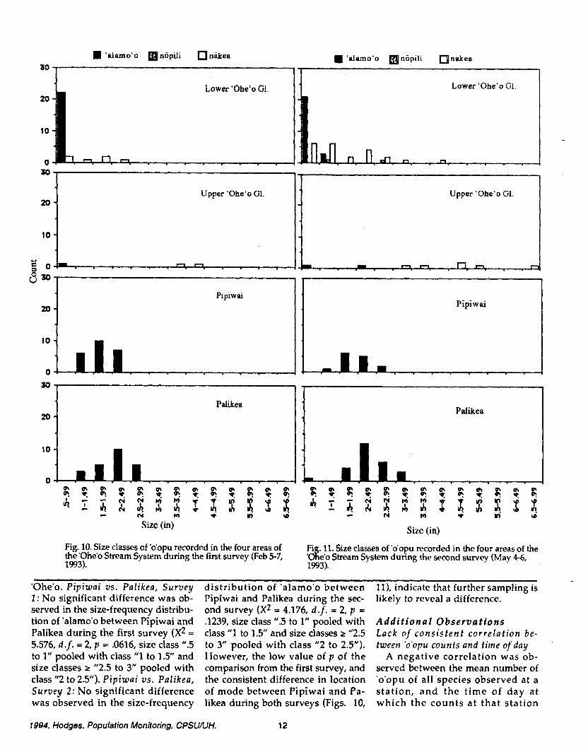
'alamo'o: Only the 'alamo'o was present in sufficient numbers to make this comparison meaningful. And, such numbers were observed in Pipiwai and Palikea alone (Figs. 10, 11). Thus, no comparison of this type '
is made involving niikea, nopili, Lower 'Ohe'o or Upper 'Ohe'o. Pipiwai: No significant difference .
was observed in the size-frequency distribution of 'alamo'o at Pipiwai between the first and second surveys (x2 = 2.532, d . f . = 2, p = .2819, size class ".5 to 1" pooled with class "1 to 1.5" and size classes r "2.5 to 3" pooled with class "2 to 2.5"). Pa-
1994. Hodges. Population Monitoring. CPSU/UH. 10

likea: No significant difference was observed in the size-frequency distri- bution of 'alamo'o at Palikea be- tween the first and second surveys (x2 = 2.261, d. f. = 3, p = .5201, size class ".5 to 1" pooled with class "1 to 1.5" and size classes r "3 to 3.5" pooled with class "2.5 to 3").
S p a t i a l Dif ferences Comparisons During Both Surveys 1 and 2 of Densities Among Areas
The 'alamo'o were observed most often in Lower 'Ohe'o, Pipiwai, and Palikea. The niikea were observed most often in Lower 'Ohe'o with some individuals in Upper 'Ohe'o. None were observed in either Pipiwai or Palikea. The n6pili were observed only in Lower 'Ohe'o. These differ- ences between areas were apparent during both the first and second sur- veys for 'alamo'o and n6pili (Fig. 8).
Comparisons During Both Surveys 1 and 2 of Size-Frequencies Among Areas
Figures 10 and 11 illustrate the distribution of sizes of 'alamo'o, nikea and n6pili in Lower 'Ohe'o, Upper 'Ohe'o, Pipiwai and Palikea during the first and second surveys. Both surveys revealed the same pat- tern. The 'alamo'o found in Lower 'Ohe'o were small and probably re- cruits. Few were observed in Upper 'Ohe'o. Larger 'alamo'o were found in Pipiwai and the largest were lo- cated in Palikea. The niikea ob- served in Lower 'Ohe'o were small with some large individuals, again probably reflecting a preponderance of recruits. Larger individuals were seen primarily in Upper 'Ohe'o. Nopili were only observed in Lower 'Ohe'o. The temporal consistency in the size frequency distribution ob- served stream system-wide is also apparent at each of these four major areas. As with the stream system- wide observations, the consistency in size frequency distribution is most apparent in the 'alamo'o. In both
F lRST SURVEY : Feb 5-7,1993 SECOND SURVEY : May 4-6,1993
30
4 'alamo'o
Size class (in) Fig. 9. Size classes of 'o'opu recorded in the 'Ohe'o Stream System during the first and second surveys (all quadrats at all stations combined).
- - -
sufficient numbers to make a formal Palikea (Figs. 10, 11). Thus, no for-
cases the increased apparent consis- tency is likely a result of a higher density and hence a larger comparison meaningful. Such numbers ma1 compa~ison is made involving size. were only observed at Pipiwai and niikea or nopili, or Lower and Upper
Only the 'alamo'o was present in
11 1984. Hodges. Population Monitoring. CPSUAJH.
. 'alamo'o nijpili n&ea 'alamo'o nopill nkkea 80
Lower 'Ohe'o GI. 20
10
0
Fig. 10. Size classes of 'o'opu recorded in the four areas of Fi .11. Size classes of 'o'opu recorded in the four areas of the the 'Ohe'o Stream System during the first survey (Feb 5-7, &e60 Stream System dunng the second survey (May 4-6, 1993). 1993).
'Ohe'o. Pipiwai v s . Palikea, Survey 1 : No significant difference was ob- served in the size-frequency distribu- tion of 'alamo'o between Pipiwai and Palikea during the first survey (x* = 5.576, d . f . = 2 p = .0616, size class ".5 to 1" pooled with class "1 to 1.5" and size classes r "2.5 to 3" pooled with class "2 to 2.5"). P i v i w a i v s . Palikea,
30-
distribution of 'alamo'o between l l ) , indicate that further sampling is Pipiwai and Palikea during the sec- likely to reveal a difference. ond survey (x2 = 4.176, d. f. = 2, p = .1239,sizeclass".5to1"pooled with Addit ional Observations class "1 to 1.5" and size classes r "2.5 Lack of c o n s i s t e n t c o r r e l a t i o n be- to 3" pooled with class "2 to 2.5"). tween 'o'opu counts and t ime o f d a y However, the low value of p of the A negative correlation was ob- comparison from the first survey, and served between the mean number of the consistent difference in location 'o'opu of all species observed at a
0 . . I I t
-
-
20 -
10 - Y
. , Survey 2 : No significant difference of mode between Pipiwai and Pa- station, and t h e time of day at was observed in the size-frequency likea during both surveys (Figs. 10, which the counts at that station
1994. Hodges. Population Monitoring. CPSUAJH. 12
Upper 'Ohe'o GI
C . . . - . . - . - r n n n -I
Upper 'Ohe'o G1.
Pipiw ai
E1 0- n n
8 30'
20 - Plpiwai
10 -

were made (Kendall's f au = -.403, Z = -2.092, p < .05). However, no such cor- relation was observed during the sec- ond survey (Kendall's tau = .la, Z = -1.065, p c .35). If a strong relation- ship between the time of day and mean 'o'opu count existed it would have been apparent during both sur- veys. There is no strong evidence to indicate that, during the daylight hours over which surveys 1 and 2 were conducted, the 'o'opu popula- tion survey protocol in 'Ohe'o need take special account of the time of day.
Inter-observer variation in 'o'opu counts Each observer counted half of the 'o'opu quadrats at each station. The question of whether different trained observers report substantially differ- ent data can be addressed to begin with by testing for a difference in the statistical distribution of each ob- server's data. There is no significant difference between myself and Brasher in the distribution of means of quadrat counts of 'o'opu recorded at each station (Counts a re of all species /sizes. First survey: Kol- mogorov-Smirnov: d . f = 2, 16 cases each survey, max difference = .188, K-S chi-square = 1.125, Z = .53, p > .60; second survey: d . f = 2, 18 cases each survey, max difference = .278, K-S chi-square = 2.778, Z = .883, p > .30).
The question may be further ad- dressed by testing whether one trained observer consistently record- ed more 'o'opu than the other. Al- though a paired t-test for a differ- ence in the mean of these station av- erages would be ideal, non-normality discourages parametric tests (see dis- cussion of zero counts above). A Mann- Whitney U test was employed. Dur- ing the first survey the mean of mean 'o'opu counts recorded by A. Brasher was .662, that of myself was .562. During the second survey that of Brasher was .411 and that of myself was .722. No significant difference in the mean of mean 'o'opu counts was detected between observers during ei- ther the first or second survey (First survey: n = 16, U = 127.5, Z = -.02, p >
.90; second survey: n = 18, U = 122, p > tween observers during both the first
.20). and second survey (First survey: n= Finally, mean observations at each 16, Kendall's tau = .624, p < .001; sec-
station were highly correlated be- ond survey: n= 18, Kendall's tau =
0 Observer 1 O Observer 2 C
FIRST SURVEY:
SECOND SURVEY: MAY 4-6, 1993 t
Fig. 12. Means of counts of all species and sizes of 'o'opu made by each ob- server at each station during the first and second surveys, 'Ohe'o Stream System. Stations ordered by distance inland but x-axis not to scale. Observ- er 1 = AB, 2 =- MH.
- -
2
March 3-5, 1 993 May 26-29. 1993
h - + I 1 U
V
bo 0 4
0 1 2 3 4 5 6 7 8 9 1011 1213141516171819202122232425
Number of '6pae per quadrat
Fig. 13. Frequency distribution of number of 'opae per quadrat in the 'Ohe'o Stream System during the first and second surveys (all stations and quadrats combined).
13 1994. Hodges. Population Monitoring. CPSU/UH.

served 12.4% change is very First survey 0 Second survey
1.2+ low (see Discussion). The non-parametric analogue failed to detect a difference between surveys 1 & 2 in the mean of raw station means (Mann-Whitney U = 111.5, 2 = -.337, p > .70).
Compar ison Between Sur- veys I and 2 of Spatial Dis- . tribution of Densi ty of En- tire Population
Figure 14 illustrates the distribution of 'Zipae in
I 500 1 000 1 500 2000 2500 3 0 0 ~ the 'Ohe'o Stream System (stations ordered by dis-
Distance inland (m) tance inland, data for sta-
Fig. 14. Distribution of "opae along the 'Ohe'o Stream System during the first and second surveys. tion 280 treated as above). The mean count of 'Gpae at cach station was well corre-
.501, p c: .005; Fig. 12). Thus, there is no evidence for aconsistent difference between Jrained observers in the na- ture of count data and the number of 'o'opu reported. This analysis does not evaluate interobserver variation where untrained observers are used. It is likely tha t such variat ion would be significant.
The 'Gpae i n 'Ohe 'o
Figure 13 illustrates the frequency distributions of quadrat counts from the first and second surveys.
Tempora l Dif ferences Comparison Between Surveys 1 and 2 of Density of Entire Population
The mean number of 'iipae of all sizes at each station during the 313- 5/93 survey ranged from 0 to 8 indi- viduals per quadrat, and the mean of these means was 3.213 (n = 15, vari- ance = 7.353, data from station 280 was the result of large recruitment event. An outlier, it was converted to zero). The mean number of '6pae of all sizes at each station during the 5126-26/93 survey ranged from 0 to 12.4 individuals per quadrat, and the mean of these means was 3.612 (n = 16, variance = 17.86).
Both of these sets of data met the definition of a 'contagious' or clumped distribution (Index of Dis- persion: x2 = 32.039, d. f. = 14, p < .05;
and X* = 74.169, d . f . = 15,p < .05 re- spectively), and were log(x t 1 )-trans- formed accordingly (Elliott 1971). Following transformation, I tested for compliance with normality. The data from the first survey conformed, but that from the second did not {Lil- liefors- First survey: n = 16, all [stan- dard normal cdf(zi) - sample cdf(zi)] and all [standard normal cdf(Zi) - sample cdf(zi,1)] < .213, p > .05. Sec- ond survey: n = 16, [standard normal cdf(z8) - sample cdf(zg)J = .219, p < .05)).
The paired-t test is powerful and somewhat robust to departures from normal assumptions. However, the power of this test to detect the ob-
lated between the first and second surveys (Kendall's t a u = .621,n = 15, Z = 3.229, p < .005).
Compnrison Between Surveys 1 and 2 of Size-Frequency of Entire Popula- tion
All netting stations combined: Fig- ure 15 illustrates the size frequency distribution of 'Gpac netted at all four netting stations in the 'Ohe'o Stream System during the first and second surveys. The observed differ- ence in frcqucncy distribution be- tween thc first and second surveys is highly significant (x* = 37.212, d. f . = 8, p = .0001; size classes 2 and 3 pooled and size classes 11,12,13
50 March 3-5, 1993
Y 40 ' 30 6 20
10
POCL (mm)
Fi .15. Post-orbital carapace Ien hs (POCL) of 'opae samples taken from f '0b during the first and sccon surveys. Samples from all netting stations pooled. Data from Station 280 removed-srch text.
1994. Hodges. Population Monitoring. CPSU/UH.
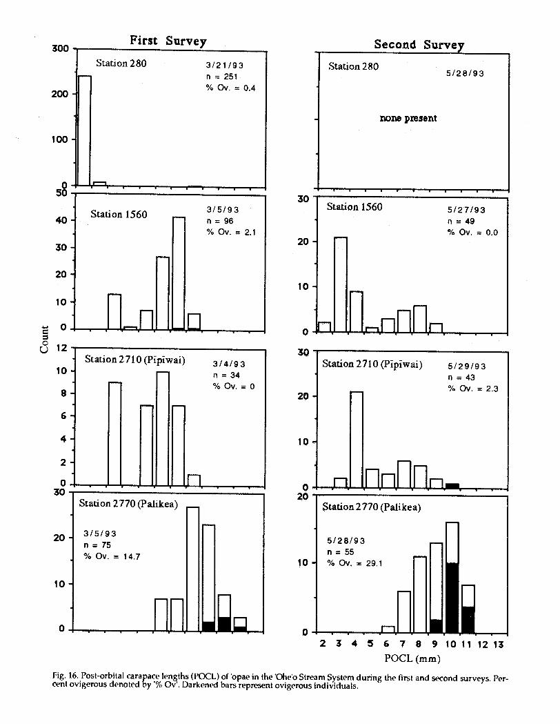
300 First Survey
Station 280 312 1 193
1 Station 2710 (Pipiwai) 3/4/9 I
I Station 2770 (Palikea)
Station 280
none present
I Station 1560
Station 2770 (Palikea)
5/28/93
2 3 4 9 6 7 8 9 1 0 1 1 1 2 1 3
POCL (mm)
Fig. 16. Post-orbital cara ace Icweths (POCL) of 'opae in the 'Ohcn'o Stream System during the first and second surveys. Per- cent ovigerous denoted g y '% Ov . Darkened bars represent ovigerous individuals.

pooled within each survey to satisfy minimum sample requirements of 2
one count for each category - e.g. Koopmans 1987, p 420; data for size class 2-3 from station 280 treated as result of large recruitment event and removed from this analysis). The analysis shows that this significant result is due primarily to the diffcr- ence at size class '2-3 mm POCL pooled' (zll = -2.490; 221 = 3.011; all other z.-< 1.960). IIowcver, some dis- ' I proportionate decrease in abundance in the larger modal size class is ap- parent in Figure 15. Other differences in size class abundance appear to be a result of a general decline in density in individuals larger than POCL 5.
Comparisons Between Surveys 1 and 2 of Sire-Frequencies From Each Net- ting Station
Figure 16 illustrates the size fre- quency distribution of '6pae netted at each of the four netting stations.
Station 280: The unusually high abundance of 2mm POCL individuals during the first survey is apparent. Absence of individuals during the second survey precludes formal com- parison.
Station 1560: The observed differ- ence in frequency distribution be- tween the first and second surveys is highly significant (x2 = 43.034, d.f. = 5, p = .0001; size classes 2,3,4 pooled and size classes 9 through 13 pooled- see above). This significant differ- ence is due primarily to differences at size classes '2,3,4 mm POCL pooled' and 8 rnrn POCL (zl = -3.076; ZZI = 4.305, zz5 = -2.538; ail other zii < 1.960).
Station 2710: The observed differ- ence in frequency distribution be- tween the first and second surveys is significant (x2 = 11.846, d. f. = 4, p = .0185; size classes 2,3,4,5 pooled and size classes 9 through 13 pooled-see above). This significant difference is due primarily to differences at size classes '2,3,4,5 mm POCL pooled', 6 mm POCL, and to a lesser extent 7 mm POCL (zll = -1.689; 212 = 1.264,z13 = 1.148).
Station 2770 (Lua Falls): The ob- served difference in frequency distri-
bution between the first and second surveys is not significant (x2 = 4.639, d . f . = 4, p = 3264; size classes 2 through 7 pooled and size classes 11 through 13 pooled-see above).
S p a t i a l Differences Comparisons During Both Surveys I and 2 of Densities Among Areas
As with 'o'opu, the relatively low number of stations in each of the four areas discourages a formal compari- son of '6pae density among these areas. However, Figure 14 illustrates the instream distribution of '6pae density. The density is fairly low in Lower 'Ohe'o, but sporadically higher throughout Upper 'Ohe'o, Pipiwai and Palikea.
Comparisons During Both Surveys 1 and 2 of Size-Frequencies Among Netting Stations
Figure 16 illustrates the size-fre- quency distribution of '6pae at each of the four netting stations. Both sur- veys 1 and 2 exhibit essentially the same pattern. Station 280 harbored no adults. Individuals recorded there appear to be recruits (POCL = 2,3). Small individuals are also found at Station 1560. The size distribution of the larger '6pae at Station 1560 is similar to that at Station 2710 (Pipiwai). The largest individuals are found at Station 2770 (Lua Falls- Palikea). None of the smaller indi- viduals recorded at the other sta- tions were observed at Station 2770.
Addit ional Observations Occurrence of Ovigerous lndividuals
The proportion of individuals ovigerous increased between surveys 1 and 2. Of the 456 individuals net- ted during the first survey, 14 (3.1%) were ovigerous. During the second survey 18 of 147 (12.2%) were oviger- ous. Although this difference in pro- portion was significant (x2 18.621, d . f. = 1, p = .0001), a ratio constructed using the number of females rather than the total number of individuals would be more instructive. The sex of sampled '6pae was not determined. Fig. 16 demonstrates that ovigerous individuals were most common at Station 2770. In addition, those
ovigero~rs tcndcd to be larger.
Lack of correlation be tween '6pae counts and time of day
No significant linear correlations wcre observcd between the mean number of 'Gpae at a station, and the time of day at which the counts at that station were made during either survey 1 or 2 (1st: Kendall's tau = - .306, Z = -1.591, p < .20; 2nd: Kcndall's tau = -.178, Z = -.962, p < .40). Yet, scattergrams of both sur- veys suggested a slight but recogniz- able decline in mean count with time of day. Although there is no strong evidence at this point to indicate that, during the daylight hours over which surveys 1 and 2 were conduct- ed, 'Zipae survey methods in 'Ohe'o need to take special account of the time of day, data from future surveys should be monitored for this possibil- ity.
The h i h i w a i i n ' O h e ' o
Hihiwai were extremely rare in the 'Ohe'o Stream System. No indi- viduals were recorded during the first and third surveys. Two individ- uals were recorded at Station 1120 during the second survey. These mea- sured 40 and 34 mm in shell length.
I Iihiwai egg cases were recorded only from Station 1120. The mean counts at 1120 wcre 5.4 (0 to 19), 6.9 (0 to 59), and 0.5 (0 to 4) egg cases per quadrat during the first, second, and third surveys respectively.
The M. lar i n 'Ohe 'o
Temporal Differences Comparison Among Surveys 1,2,3 and 4 of Abundance of Entire Population
The mean number of M. lar in each trap during the first survey was 3.04 (variance = 8.63, range: 0 to 11, n = 28, C = 85); during the second: 5.96 (var =
19.40, range: 0 to 16, n = 26, C = 155); the third: 11.3 (var = 86.642, range: 0 to 39, n = 20 C = 226); the fourth: 7.07 (var = 43.624, range: 0 to 29, n = 28, C = 198). Mcans were significantly dif- ferent among surveys (ANOVA ap- plied to log(x+ 1)-transformed number per trap, p < .0001). The detrans-
1994. Hodges. Population Moniloring. CPSUAJH. 16

J a m ary April July November 40 0 I
Fig. 17. Numbers of M. lar trapped in the 'Ohe'o stream system (n = number tra set, f = total number M lar trapped). The means of surveys 1,2 and 3 are signir cant y different from each other. The mc.an of survey 4 is different from 1 but in- distin ishable from 2 and 3 (see capital letters - comparison of survey means uingf?sherrs Least Significant Difference, p < .05).
S p a t i a l D i f f e r e n c e s Comparisons Among Surveys 1 , 2 , 3 and 4 of Abundances Among Areas
Differences in abundance among areas were not consistent:
first: The mean number of M. lar trapped in Upper 'Ohe'o, Lower 'Ohe'o, Pipiwai and Palikea were 5.4, 1.67, 1.6, and 2, respectively. This difference was significant (log(xt 1 ) transformed, ANOVA, d. f. between = 3, d . f . within = 24, p =
,0145; significance due to differences between Lower and Upper 'Ohe'o, and between Lower 'Ohe'o and Pipiwai, Fisher's LSD, p < .05). second: The mean number of M. l a r trapped in Upper 'Ohe'o, Lower 'Ohe'o, Pipiwai and Palikea were 7.7, 2.1, 10.8, and 2.5, respectively. This difference was significant
formed means using the variance cor- p c .01; Survey 2 vs. Survey 4: transformed, d . ~ rection of Elliott (1970) are 3.1, 6.3, Kendall's tau = ,534, n = 26, Z = 3.822, between = 3, d . f , with in = 22, = 12.3, and 7.2. P .0005; vs. 4: ,0001; the only non-significant pair-
The mean number of M. lar per Kendall's tau = .474, n = 20, Z = 2.921, wise comparisons were between trap increased significantly between p < .005). Lower 'Ohe'o and Pipiwai and be- the first and second, and second and tween Upper 'Ohe'o and Palikea, third surveys. The mean of the Comparisons Among Surveys 1, 2 , 3, Fisherrs LSD, < .05). fourth survey was significantly dif- and 4 of Mean Size of Entire Popula- third: The mean number of M , lar ferent from that of the first survey t ion trapped in Upper 'Ohe'o, Lower only (Fisher's LSD, p < .05, Fig. 17). The the mean P°CL(mm) 'Ohe'o, and Pipiwai were 13, 6.29,
The total number of males trapped of those trapped at each station dur- and 16, respectively. No data was increased from 117 to 163 and again to ing the first survey was 32.2 (var = collected in Palikea. This difference 166 during the second, third and 101.7, range: 11 to 46, n = 24 stations); not significant trans- fourth trappings. The number of fe- second: 34.0 (var = 58.2, range: 18 to formed, ANOVA, d . f , between = 2, males trapped increased from 28 to 45.6, n = 24); third: 34.9 (var = 53.5, d . f , within = 17, = .0874). 59, then declined to 30. Thus the range: 14 to 45.5, n = 19); and f~u r th : The mean number of l a y overall increase between the second 33.6 (var = 54.3, range: 16.5 to 45.5, n t rapped i n Upper . ~ h ~ ~ ~ , Lower and third trappings appears due to = 27). These differences among sur- .Ohe.o, Pipiwai and Palikea were both males and females. veys in the mean of mean size at each 8.8, 4.7, 9, and 5.7, respectively This
station were significant difference was significant (log(xt1) Comparison Among Surveys 1 , 2 , 3 (ANOVA,p = ,7459). transformed, ANOVA, d. f . between = a n d 4 of S p a t i a l D i s t r i b u t i o n of 3, d . f . within = 24, p = ,304). Abundance of Entire Population Comparisons Among Surveys 1 , 2 , 3,
The number of prawns trapped at and 4 of S i ze -Frequency of Ent ire Compnrisons Among Surveys 2, each station during the first survey Population and 4 of S i z e - F r e q u e n c i e s A m o n g was not significantly correlated to All stations combined: Figure 18 il- Areas that of Surveys 2.3. and 4. However, lustrates the size frequency distribu- The size frequency distribution of Surveys 2,3, and 4 were significantly tion of M . lar trapped throughout the M . l a , differed among Lower ohe.o, intercorrelated (Survey 1 vs. Survey 'Ohe'o Stream System during the Upper .Ohe.o, Pipiwai and palikea 2: Kendall's t a u = .23, n = 26, Z = four surveys. The differences in size (Fig. 19). differences were con- 1.646, p < .lo; Survey 1 vs. Survey 3: frequency distribution among the sur- sistent for the most part. o ow ever, Kendall's t a u = .28, n = 20, Z = 1.727, veys are significant (two smallest the mode a t .oheao shifted p < .lo; Survey 1 vs. Survey 4: size classes pooled to satisfy mini- ,ticeably upwards between the set- Kendall's t a u = .244, n = 28, Z = 1.821, mum sample requirements-see above, and third surveys, p < .lo; Survey 2 vs. Survey 3: 4 x 9 matrix, x2 =42.229, d . f . = 2 4 p = Kendall's t a u = 4 1 , n = 20, Z = 2.721, .0122).
17 1994. Hodges. Population Monitoring. CPSU/UH.

30 January 1-3, 1993 n traps = 28
= 85 n traps = 26
n male = 117 n female = 28 n ? = 1 0 m:f ratio = 4.2 n
aunknown gender males non-ovig. females ovigerous females
1 November 20-23, 1993 n 1
n male = 166 n female = 30
m:f ratio = 5.5 % females ovi-
= 226 n male = 163 n female = 59 n m:f ratio = 2.8 % females ovi- gerous = 57.6
-. - -. . - ~ c u c u ~ m G w m m v v v v v v v v v v X X X x X X X X X X x x x x x x x x x x
8 t : X # # # $ # C 1-
Post-Orbital carapace length (mm)
Fig. 18. Lengths and related statistics of Macrobrachiurn lar durin surv trapping in the 'Ohc'o stream system, Kipahulu, Maui. Sizes of male, nonovigerous and ovigerous female, and in&idu% of undetermintbd gender are indicated.
A d d i t i o n a l O b s e r v a t i o n s nificantly different among Surveys -0.128, Z = -0.787, p > .40; fourth: n = Comparisons Among Surveys 1 , 2 , 3 and 4 of Sex Ratio and Percent Ovigerous
Sex was not recorded during the first survey. The sex ratio (m:f) was 4.2, 2.8, and 5.5 during Surveys 2,3,and 4 respectively. The differ- ence among these was significant (x2 = 8.289, d . f . = 2, p < .0159; Fig. 18) and was caused primarily by an ex- cess of females over that expected by chance during Survey 3 and a deficit of females over expected during Sur- vey 4 ( z l l = .215, 212 = -.388; 221 = - .970, 222 = 1.895; ~ 3 1 = .861, ~ 3 2 - - 1.681).
Likewise, the proportion of fe- males which were ovigerous was sig-
2,3 and 4 (x* = 29.493, d.j . = 2, ;= .0001; Fig. 18). This difference in the proportion ovigerous was caused pri- marily by a deficit over expected of ovigerous females during Survey 2, but also by an excess of ovigerous fe- males over expected during both Sur- veys 3 and 4 ( z l = -3.527,q2 = 3.154; 221 = 1.519, 222 = -1.359; 231 = 1.279, 232 = -1.144)
27, tau = -.067, Z = -.488,p > .60). During both the third and fourth
surveys, the proportion of individu- als in each t rap which exhibited symptoms of "black-spotted disease" showed no linear correlation with ci- ther the number (third: Kendall's tau = 0.1, Z = 0.666, p > SO; fourth: n = 27, tau = .104, Z = .762, p > .40), or the mean carapace length (third: Kendall's tau = 0.165, Z = 0.986, p > .4O;/ourth: tau = 0.067, Z = 0.491, p > .50) of individuals in the trap. A n ex- amination of the corresponding scat- tergrams indicated that no simple non-linear correlations were likely.
Data from the third survey show a clear tendency for increased incidence
lncidence of "black-spotted disease" The proportion of individuals in
each trap which exhibited symp- toms of "black-spotted disease" showed no correlation with the dis- tance inland (m) of the trapping lo- cation (third: n = 18, Kendall's tau =
1994. Hodges. Population Monitoring. CPSUIUH. 18

Lower @OheCo Upper 'Ohc'o Pipiwai Palikea 20 5 4 3
4 3 3 2
* 10
b W
2 2
1 1 1
0 0 0 0
Fig. 19. Size fre uency distributions of M. lar trapped in Lower 'Ohe'o, Upper 'Oheo, Pipiwai, and Palikea during the first, sec- ond, third and &rth surveys. Note differing axes.
of symptoms with size. This pattern = 28 to 51 mm, mean carapace length ing the third and fourth surveys was was not as clear during the fourth = 41.9 mm, Fig. 20). The mean cara- independent of distance inland, and (Fig. 20). In both cases, however, in- pace length of individuals exhibit- the number and mean size of individ- dividuals of both sexes exhibiting ing symptoms was significantly uals in each t rap. However, al- symptoms of "black-spotted disease" greater than that of those without though large individuals were during the third and fourth surveys symptoms (no symptoms: n = 180, trapped which showed no symptoms, were among the larger of all individ- range in carapace length = 9 to 55 those individuals which exhibited uals trapped during those surveys mm, mean carapace length = 34.9 mm; symptoms were significantly larger (all traps combined; n-225,rangein Mann-Whitney U = 2174.5, Z = - than those which did not. carapace length = 9 to 55 mm, mean 4.806, p < .00001). carapace length = 36.3 mm; symp- Thus incidence of symptoms of toms: n = 45, range in carapace length "black-spotted disease" per trap dur-
19 1994. Hodges. Population Monitoring. CPSU/UH.

Males 50
July 17-19, 1993 35.6 n 1 Females
I 1
1 no symptoms symptoms I
O V ) O V ) O V ) O V ) O V ) r v - ( Y ( Y O C 9 b U V ) V ) v v v v v v v v v v X X X X X X X X X X ~ O ~ O V ) O U ) O V ) O
r r ( U C V O O b W V )
Post-orbital carapace length (mm)
Fig. 20. Lengths of M. lar exhibiting symptoms of 'black-spotted disease' during survey trappin 'Ohe'o Gulch, Kipahulu, Maui. Percentages of individuals rrhibit~ng symptoms in each size class are indicated. Note dit%"ng axes.
Number trapped not correlated w i t h viduals in each trap showed no lin- > 30; fourth: n = 28, t au = -.019, Z = - mean s i z e t rapped
The number of individuals per trap showed no linear correlation with the mean carapace length in each trap (first: n = 24, Kendall's t a u = - .039, Z = -.27, p > .70; second: n = 24, tau = ,105, Z = .721, p > .40; third: outlier at station location 1630 re- moved, n = 18, tau = ,047, Z = 0.273, p > .70; fourth: n = 27, tau = .254, p >.05, though slight curvilinearity apparent, result no different for l og (# trapped)).
Mean POCL not correlated with dis- tance inland
The mean carapace length of indi-
ear correlation with distance inland (first: n = 24, t au = 0, Z = 0, p -> unity; second: n = 24, tau = -.OBI Z = -546, p > .50; third: outlier at station loca- tion 1630 removed, n = 20, tau = - 0.216, Z = -1.294, p > .lo; fourth: n = 27, tau = -.169, Z = -1.237, p > .lo).
Number trapped not s t rongly corre- lated w i t h d is tance inland
The number trapped was negative- ly correlated with distance inland during the first (n = 28, Kendall's t au = -.323, Z = -2.41, p < .02); but not so during the remaining surveys (second: n = 26, tau = -.032, Z = -.228, p > 30; third: n = 20, t au = -.027, Z = -.166, p
N u m b e r of hours t r a p i n w a t e r not consis tent ly related to number of M . lar t rapped During the first, sec- ond, third, and fourth surveys the traps remained in the water for 14.5 to 19, 17.5 to 20, 15 to 18.5, and 17 to 18.5 hours respectively. The mean number of hours the traps were in the water differed significantly among the four surveys (mean of 1st = 17.3, 2nd = 18.4, 3rd = 17.0, 4th = 17.6; Kruskal Wallis: d . f . = 3, H = 16.869, p < .001).
The number of M. lar trapped de- clined significantly with the number
1994. Hodges. Population Monitoring, CPSUAJH. 20

March July 4 Oct. 5-6 Oct. 6-7 Dec. 4 20-2 1 26- 9
1.6- I I I o I I I MY .- , Lower I
1.4. o I Lower Pua'alu'a a I 'Ohe'o ,
0 1 2. I
Fig. 21. Densities of '0'0 u and 'opae in lower Pua'alu'u and lower 'Ohe'o (see text). Note recruit pulse at '0hhe.o Station &I removed from above graph).
in the numbcr or mean numbcr of M. trapped is unlikely to have been a function of trapping time.
T h e ' o ' o p u i n P u a ' a l u ' u
The mean numbers of 'o'opu of all species and sizes were 2.7, 4.2, 3.3, and 4.0 individu- als per quadrat during the first, second, sec- ond-repeat, and third surveys respectively (n=30 in each in- s tance) . Elliott's (1971) Index of Dispcr- sion categorized the distributions of the first, second and third surveys as 'clumped' and that of the second- repeat as 'random' (comparatively little distance among sta- tions indicated concern over hierarchy of spa- tial autocorrelation here unnecessary, thus quadrat counts pooled among stations;x2 =
75.7, 72.7, 164.0 and 43.1 respectively; d . f. = 29 in all cases). The full data set could not be normalized. Using the nonparametric analogue, the mean number did not differ significantly among the four surveys (see above rationale for
of hours the trap was in the water mained in the water during the pooling of quadrat counts. Kruskal- during the first survey (n = 28. fourth survey showed no apparent d.f. = 3, = 4,617, p , Kendall's tau = -.544, Z = -4.061, p c linear relationship with the number .OOOl). but was not significantly ;or- of M. lor trapped. Also, though the The + l p i n Pu a a l u . related with the number of hours s a m ~ l e size is small there is a lack of during either the second (n = 26, Kendall's t a u = ,068, Z = .486, p c .70), or third (n = 28, Kendall's tau = -.102, Z = -.63, p c .60) surveys. The small range of the number of hours discourages a correlation computa- tion for the fourth survey, however the number of hours the trap re-
both any visible or significant rela- tionship between the mean number trapped (see above) and the mean number of hours (n = 4, Kendall's t au = -.333, Z = -.609, p < .60). Thus, al- though the mean trapping times dif- fered, over the range of trapping times used any observed differences
(See above discussion of effect of new personnel employed during third survey). The quadrat counts from the 2nd-repeat and third surveys appear to have arisen from a common distri- bution (Kolmogorov-Smirnov: d.f = 2, 30 cases each survey, max difference = .233, K-S chi-square = 3.267, Z =
21 1994. Hodges. Population Monitoring. CPSUNH.

HIHIWAI Jan March
July 4 Oct. 5-6 Oct. 6-7 Dec. 4 19-21 20-21 26- 9 .5 .- Mar
I I I I I I .- Lower I Lower
Pua'alu'u '0he ' o .35
0 0
.25
.15
.05 ........ .... ...... 0 ..- ........ ........ -" - !..-..,...- -...
n = 3 0 n = 3 0 n = 3 0 n - 3 0 n = 3 0 n = 3 0 n = 3 0 = 2 = 8 = 2 = 3 = 0 = 0 = 0
HIHIWAI EGGS
' O h e ' o vs. P u a ' a l u ' u
Densities of 'o'opu, . - opae, h ih iwai and hihiwai egg cases were higher in Ptla'alu'u than in 'Ohc'o (Figs. 21, 22; no formal comparison). Al- though, Pua'alu'u sur- veys were not concurrent with 'Ohe'o, the rela- tive temporal consistency of the data sets indicates that the differences are real.
DISCUSSION
T h e ' o ' o p u i n '0 h e ' o
the results do not seem to n = 3 0 n = 3 0 n = 3 0 n = 3 0 n = 3 0 n = 3 0 n = 3 0 be consistently affected
= 18 = 32 = 7 6 = 2 1 3 = 0 = 0 = O by the time of day in
M e t h o d Jan March
July 4 Oct. 5-6 O a . 6-7 Dec. 4 19-21 20-21 g a l g The results indicate 2 .25 I 1 I t I
that the direct observa-
Fig. 22. Densities of hihiwai and hihiwai eggs in lower Pua'alu'u and lower 'Ohe'o (see text). which the counts are made.
.904, p > .30). and 35. It is unknown whether these The mean numbers of '7ipae were counts are accurate. However, both W i t h i n - s t r e a m o f
2.5, 2.0, 2.4, and 5.3 individuals per were reported by the newer person- ' O * O P U Spec ies quadrat during the first, second, sec- nel. Fitzsimons and Nishimoto (1991) - ond-repeat, and third surveys respec- describe what can be viewed as the tively (n=20 during first, n = 30 dur- The h i h i w a i i n Pua'alu'u typical instream distribution of ing following). No significant differ- 'o'opu: akupa are found in the lower ence was detected among these sur- Hihiwai were present in low abun- reaches; n o ~ i l i are found from the veys (Kruskal-Wallis: d.f. = 3, H = dance. The mean numbers recorded lowcr waches the mid 3.041, p > .25). were .067, 2.0, 2.4, and 5.3 individu- nakea Occur in the lower, mid, and oc-
A look at Appendix I1 shows that als per quadrat respectively (n=20 casionally reaches; and the mean value for the third survey during first, 30 in latter). 'alamo'o are most often found in the is inflated by two observations: 25 upper reaches. Because 'o'opu species
may differ in their climbing ability
, tion method provides re- alistic data: The strong correlation between both
: surveys 1 and 2 in the . mean number of 'o'opu
counted at each station : indicates that the sur- . vey method employed I detects actual spatial
differences in 'o'opu . abundance. These spa-
also tial detected differences by differ- were ent observers. Further,
I
2 Lower 0 ; Lower
1994. Hodges. Population Monitoring. CPSUIUH. 22
1.75.
1 .5. 4
1.25
Pua'alu'u I 'Ohe'o I
I 0 a
0 0 :
0
o
.25 l...... b ....... ....... 0 ... ...... .. I...- - -...,

(e.g. Nishimoto 1992), this ideal in- stream distribution may be strongly influenced by geomorphological fea- tures such as waterfalls (e.g. Ford 1979).
The distribution of 'o'opu in 'Ohe'o follows this model. Akupa were not recorded, and could have been re- stricted from entry into 'Ohe'o by the - small terminal waterfall. The tiny handful of n6pili recorded were in Lower 'Ohe'o. The n5kea were recorded in Lower and Upper 'Ohe'o. All adult 'alamo'o were located in Pipiwai and Palikea.
G e n e r a l l y l o w a b u n d a n c e b u t s i g n i f i c a n t ' a l a m o ' o
In comparison with what I have observed in high-quality streams such as Hanawi, Wailau, Waikolu, and Hanakapi'ai, the densities of hihiwai, 'Gpae, and 'o'opu in the 'Ohe'o Stream System were general- ly low. However, the densities of 'alamo'o in certain areas were the highest I have seen anywhere in Hawai'i. Ind iv idua l 'a lamo'o a t these locations are also the largest I have seen.
The ' i i pae i n ' O h e ' o
The apparent general decline in density in individual '6pae larger than POCL 5 observed from netting data suggests that the destructive sampling may be the cause of decline. Caution is advisable. Future surveys should rely on live measurements, es- pecially if the sampling interval will be short and/or the population abundance is similar to that observed in the first and second surveys.
The h i h i w a i i n ' O h e ' o
During preliminary reconnaissance at the initiation of this study, al- most the entire channel length of the study area was visually examined. During both reconnaissance and sub- sequent survey work, hihiwai were observed at only two locations. A sin- gle spat was seen near Station 40 dur- ing reconnaissance. A very small number of adults (estimated at 20- 100) was observed at a small section
of boulder riffle at Station 1120 dur- ing reconnaissance. The only hihiwai recorded during a survey were at Station 1120. The density recorded was very low. Egg cases were also observed only at Station 1120 during reconnaissance, and were recorded only at Station 1120 during the three surveys.
The mean number of adults (.20) recorded at Station 1120 compares well with the mean number of adults per station recorded in Waiohue (.65), Honomanu (.09), and Hanawi (-49) Streams during 1991 (Hodges 1992). Likewise, the mean number of egg cases recorded during each of the three surveys (5.4, 6.9, .50) at Station 1120 compare well with the mean number of egg cases per station recorded in these other streams (4.1, .9, 6.9 respectively). Unlike these other streams, however, the hihiwai and egg cases in 'Ohe'o occur only at one small location rather than throughout the stream.
Kinzie and Ford (1977) stated that hihiwai were present at locations in 'Ohe'o which correspond roughly to Stations 130,160,990, and 1120. Kinzie and Ford gave no quantities with which to compare present ob- servations. However, both reconnais- sance in the areas examined by Kinzie and Ford, and subsequent sur- veys in identical or very nearby loca- tions, indicate that hihiwai are no longer as widely distributed as they were during the time of Kinzie and Ford's observations.
The M . l a r in ' O h e ' o
Abundance The abundance of M. lar in 'Ohe'o
cannot be quantitatively compared to that of other streams until a stan- dardized method using the same or similar gear is applied in other streams. However, based qualitative observations I have made in a large number of streams throughout Hawai'i, M. lar appears quite abun- dant in 'Ohe'o. A. Brasher (pers. comm. - 1994) suggests that abun- dance of this species increases with increasing temperature and increas- ing availability of pool habitat .
This appears likely.
Incidence of "black s p o t t e d d is - ease"
Kubota (1972) noted that Kahana Strcam and estuary, O'ahu was the only stream thus far investigntcd in IIawai'i in which symptoms of 'black-spotted disease' had been hund on M. lar. of the M . lar that he worked with from Kahana 17.4% ex- hibited symptoms. The incidence fre- quency of symptoms in 'Ohe'o is very similar to that observed in Kahana. During the third and fourth surveys respectively, 20.0% and 15.7% of those trapped in the 'Ohe'o Stream System exhibited symptoms.
Edfect of M . l a r on n a t i v e am- ph idromous fauna
During the course of the surveys it was very common to observe M . lar displacing '6pae and 'o'opu by ap- parently aggressive movement into the spaces occupied by the '6pae and 'o'opu. I Iigh densities of M. lar must pose a bioenergetic cost to natives from frequent displacement and in- terruption of feeding and mating ac- tivities.
The M. lar may also be a signifi- cant predator of natives. Kubota (1972) suggests that M. Iar t ake 'o'opu egg masses, and reports inci- dences of M. lar taking adult 'o'opu both in the aquarium and in s i tu . In one case, Anne Brasher and myself observed an M. l a r feeding on the head of an 'o'opu niipili during the night in Waikolu Stream on Molo- ka'i. The head was retrieved and was not at all decomposed. In addi- tion, M. lar were observed by Anne Brasher and myself on a number of oc- casions feeding on adult hihiwai in Waikolu Stream. The effects of M. l a r on the native amphidromous fauna is a critical area for future study.
C o n t r o l If M, lar is shown to have a strong
adverse effect on native species it may be desirable to initiate a control program in 'Ohe'o. The data gath- ered in this study will provide an amplc baseline with which to evalu-
31 1994. Hodaes. Po~ulation Monitoring. CPSUAJH.
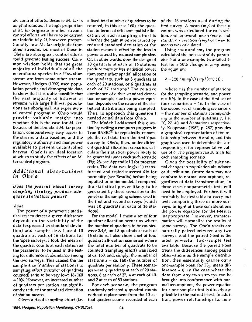
ate control efforts. Because M. lar is amphidromous, if a high proportion of M. lar originate in other streams control efforts will have to be carried out indefinitely. If, however, propor- tionally fcw M. lar originate from other streams, i.e. most of those in 'Ohe'o are aboriginal, control efforts could generate lasting success. Com- mon wisdom holds that the great majority of individuals of all the macrofauna species in a Hawaiian stream are from some other stream. However, Hodges (1992) used popu- lation genetic and demographic data to show that it is quite possible that the vast majority of hihiwai i n streams with large hihiwai popula- tions are aboriginal. An experimen- tal control program in 'Ohe'o would provide valuable insight into whether this is the case for M. far . Because of the abundant M. lar popu- lation, comparatively easy access to the stream, a data baseline, and the regulatory authority and manpower available to prevent uncontrolled harvest, 'Ohe'o is an ideal location at which to study the effects of an M. 1 a r control program.
A d d i t i o n a l o b s e r v a t i o n s i n ' O h e ' o
Does the present v i s u a l s u r v e y s a m p l i n g s t r a t e g y produce ade- q u a t e s t a t i s t i c a l power?
' i ipae The power of a parametric statis-
tical test to detect a given difference depends on the variability of the data (expressed as standard devia- tion) and sample size. I used 10 quadrats at each of 16 stations for the '6pae surveys. I took the mean of the quadrat counts at each station as the parameter to be used in the test- ing for difference in abundance among the two surveys. This caused the the sample size (number of stations) to sampling effort (number of quadrats counted) ratio to be very low: 161160 = 10%. However, an increased number of quadrats per station can signifi- cantly reduce the standard deviation of station means.
Given a fixed sampling effort (i.e.
a fixed total number of quadrats to be counted, in this case 160), the ques- tion in terms of efficient spatial allo- cation of such sampling effort is whcther the gain in powcr causcd by rcduccd standard deviation of the station means is offset by the loss in power caused by reduced sample size. Or, in other words, does the design of 10 quadrats at each of 16 stations produce more or less statistical power than some other spatial allocation of the quadrats, such as 8 quadrats at each of 20 stations, or 6 quadrats at each of 27 stations? The relative dominance of either standard devia- tion or sample size in a power equa- tion depends on the nature of the sta- tistical distribution being sampled. Thus, to approach this question I needed actual data from 'Ohe'o.
Thc Model: I addressed this ques- tion by writin a computer program in True BAS1 '@ to repeatedly re-sam- ple the real data from the first '6pae survey in 'Ohe'o, then, under differ- ent quadrat allocation scenarios, cal- culate the statistical powcr likely to be generated under each such scenario (Fig. 23, see Appendix I11 for program code). The data was log(xt1) trans- formed and tested successfully for normality (see Results) before being inputted in to the model. I compared the statistical power likely to be generated by these scenarios to the power of the sampling scheme used in the first and second surveys (which was 10 quadrats at each of 16 sta- tions).
For the model, I chose a set of four quadrat allocation scenarios where the number of quadrats to be counted were 2,4,6, and 8 quadrats at each of 16 stations. I also chose a set of four quadrat allocation scenarios where the total number of quadrats to be counted (sampling effort) was fixed at ca. 160, and, simply, the number of stations x = ca. 160/the number of quadrats per station y . These scenar- ios were: 8 quadrats at each of 20 sta- tions, 6 at each of 27,4 at each of 40, and 2 at each of 80 stations.
For each scenario, the program randomly selected y quadrat counts without replacement from the 10 ac- tual quadrat counts recorded at each
1994. Hodges. Population Monitoring. CPSUM. 24
of the 16 stations used during the first survey. A mean (my) of these y counts was calculated for each sta- tion, and an overall mean (m my) and standart1 deviation (srrry) of thcsc I6 means was calculated.
Using tnmy and s t ~ y the program calculated the non-centrality param- eter a of a one-sample, two-tailed t- test for a 50% change in nznry using the cquation:
where x is the number of stations for the sampling scenario, and power IT = f(a). In the case of the first set of four scenarios x = 16. In the case of the second set of sampling scenarios x = the number of stations correspond- ing to thc number of quadrats y; i.e. 20, 27, 40, and 80 stations respective- ly. Koopmans (1987, p. 287) provides a graphical representation of the re- lationship between a and n, and this graph was used to determine the cor- responding n for rcpresentative val- ues of 3. Thc program ran 30 trials for each sampling scenario.
Given the possibility of substan- tial changes in population abundance or distribution, future data may not conform to normal assumptions, re- gardless of data transformation. In these cases nonparametric tests will need to be employed. Further, it will probably bc desirable to carry out tests comparing three or more sur- veys. In light of these considerations the power equation for the t-test is inappropriate. IIowever, transfor- mation will normalize the results of some survcys. The 'Ohe'o results are naturally paired between any two surveys, and the paired t-test is the most powerful two-sample test available. Because the paired t-test treats the differences among paired observations as the sample distribu- tion, then essentially carries out a one-sample t-test for HI: mean dif- ference * 0, in the case where the data from any two surveys can be brought into conformance with nor- mal assumptions, the power equation for a one-sample t-test is directly ap- plicable to the paired t-test. In addi- tion, power relationships for non-

y number of quadrats at each of x number of stations
total number of quadrats Fig. 23. Non-centrality parameter (a) as a function of the number of quadrats per station (y) and the num- ber of stations (x) from hy thetical '6pae surveys in 'Ohe'o, Ki ahulu. The value of a calculated from t: the actual obscrvatiom m a g during the first 5 ae survey in e'o is at the center of the diagram (sam- pling design: 10 quadrats at each of 16 statiom)he other values of 3 were calculated from simulations of various sampling scenarios using the count data of the first '6pae survey (see text). The four data sets on the left of center are the likely values of a iven the hypothetical sam lin scenarios of 2, 4, 6, and 8 quadrats at each of 16 stations respectively. h e four data sets on the ri Kt of center are the likely values 9 of a given the h othetical samplmg scenarios of 8 quadrats at each of 0 stations, 6 quadrats at e a h of 27 stations, etc. R e total number of uadrats which each h thetical samplin scenario entails are indi- TP" B cated on the lower horizontal axis. &e set of a enerated or each hypothetica sampling scenario is the result of 30 trial runs. Representative values of &e power (n) of a one-sample, two-tailed t - test, where the difference to be detected is * 50% of the population mean, corresponding to a are indicated on the right vertical axis.
parametric tests are very difficult to establish (Sprent 1993, p. 297). And, power calculations for tests involving three or more samples (e.g. ANOVA) require data from an additional sur- vey beyond the two carried out to date. Consequently, I used the power relationship for the one-sample t- test in this model to a) provide a guideline for the planning of future sampling strategies where the t-test proves appropriate, and b) to gain in- sight into the relative difference~ in power likely to be generated by the different sampling scenarios regard- less of the test to be employed.
Model results: Figure 23 displays the results of the simulations for each sampling scenario. For the first set of four sampling scenarios (y varies but xis fixed at 16) a decreases as y decreases. This is caused by an increase in smy with decreasing y.
However, once x is allowed to in- crease in proportion to the decrease in y, a increases with the decrease in y. Thus, the change in sample size x has a greater effect on a than the cor- responding change in y. In other words, for the nature of the statisti- cal distribution of quadrat counts of 'iipae at 'Ohe'o, the power of a t-test improves as the number of stations increases, even if the number of quadrats at each station decreases proportionally.
Figure 23 also illustrates represen- tative values of n for the corresgond- ing a. The actual data from the first 'Zipae survey yield a very low n. Only the scenarios 4 63 40 and 2 d 80 yield n 2 the standard .90.
A large number of quadrats at each station has a number of advantages. More quadrats per station allow a more meaningful comparison of obser-
vations among sta- tions. In instances of low population abundance, as has bccn obscrvcd in 'Ohc'o, more quadrats per station mean fcwcr station means which equal zero and thus a greater chance that t r a n s f o r m a t i o n s will bring station means in confor- mance with normal assumptions. The meeting of such as- sumptions allow application of the more powerful parametric meth- ods. Of course, the sampling scenario model I used de- pended on a com- para t ive ly large number of quadrats per station from which to re-sam- ple. These benefits aside, the very low power observed for the first '6pae sur- vey indicates that future surveys fo-
cussing on changes in population abundance should utilize far more stations than the 16 used in the first and second surveys. The model demonstrates that for the case of 'Zipae in 'Ohe'o, sufficient power for a t-test will be achieved, for the same sampling effort as applied at present, by using 40 to 80 stations with a corresponding decrease in the number of quadrats per station.
'o'opu The same model as that used for
'Zipae was used for 'o'opu. Quadrat counts from the second survey in 'Ohe'o were transformed as the square root of (x + 0.05) and tested successfully for normality (Lilliefors: p > .05) before being used in the model.
The relative results are much the same as for 'Zipae (Fig. 24). Where
25 1994. Hodges. Population Monitoring. CPSUNH.
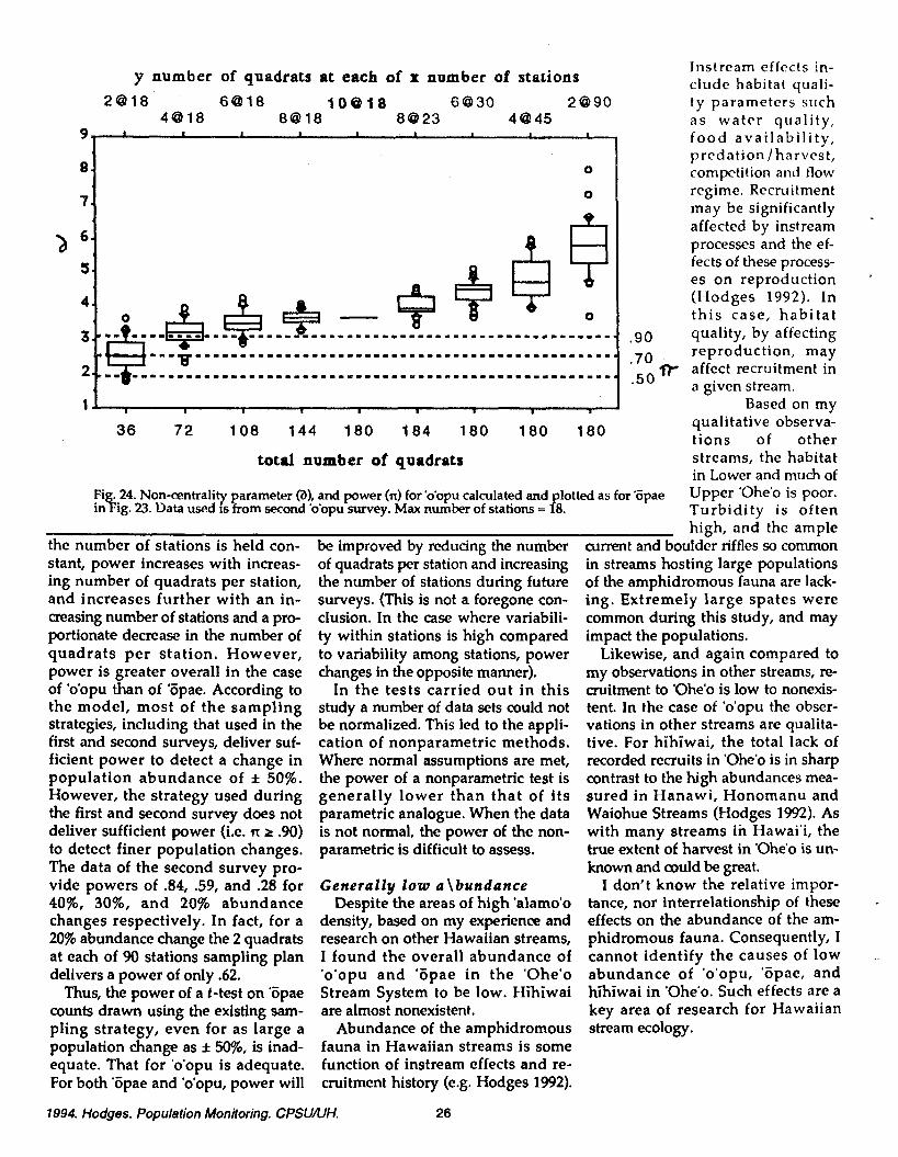
y number of quadrats at each of x number of stations Instream effects in- clude habitat quali- ty parameters such as water quality, food availability, predation /harvest, competition and flow regime. Recruitment may be significantly affected by instream processes and the ef- fects of these process- es on reproduction . (Hodges 1992). In th is case, habitat
-90 quality, by affecting reproduction, may
.Tr affect recruitment in s 5 0 a given stream.
Based on my qualitative observa- tions of other
total number of quadrats streams, the habitat in Lower and much of
Fi .24. Non-centrality parameter (a), and power (n) for 'obpu calculated and lotted as for 6pae Upper 'Ohe'o is poor. % in 4g. 23. Data used is from second 'obpu survey. M u number of stations = P8. Turbidity is often
the number of stations is held con- stant, power increases with increas- ing number of quadrats per station, and increases further with an in- creasing number of stations and a pro- portionate decrease in the number of quadrats per station. However, power is greater overall in the case of 'obpu than of '6pae. According to the model, most of the sampling strategies, including that used in the first and second surveys, deliver suf- ficient power to detect a change in population abundance of * 50%. However, the strategy used during the first and second survey does not deliver sufficient power (i.e. n r 9 0 ) to detect finer population changes. The data of the second survey pro- vide powers of .84, .59, and .28 for 40%, 30%, and 20% abundance changes respectively. In fact, for a 20% abundance change the 2 quadrats at each of 90 stations sampling plan delivers a power of only .62.
Thus, the power of a t-test on '6pae counts drawn using the existing sam- pling strategy, even for as large a population change as ;t SO%, is inad- equate. That for 'o'opu is adequate. For both '6pae and 'o'opu, power will
be improved by reducing the number of quadrats per station and increasing the number of stations during future surveys. (This is not a foregone con- clusion. In the case where variabili- ty within stations is high compared to variability among stations, power changes in the opposite manner).
In the tests carried out in this study a number of data sets could not be normalized. This led to the appli- cation of nonparametric methods. Where normal assumptions are met, the power of a nonparametric test is generally lower than that of its parametric analogue. When the data is not normal, the power of the non- parametric is difficult to assess.
Generally l o w a \bundance Despite the areas of high 'alamo'o
density, based on my experience and research on other Hawaiian streams, I found the overall abundance of 'o'opu and '8pae in the 'Ohe'o Stream System to be low. Hihiwai are almost nonexistent.
Abundance of the amphidromous fauna in Hawaiian streams is some function of instream effects and re- cruitment history (e.g. Hodges 1992).
high, and the ample current and boulder riffles so common in streams hosting large populations of the amphidromous fauna are lack- ing. Extremely large spates were common during this study, and may impact the populations.
Likewise, and again compared to my observations in other streams, re- cruitment to 'Ohe'o is low to nonexis- tent. In the case of 'o'opu the obser- vations in other streams are qualita- tive. For hihiwai, the total lack of recorded recruits in 'Ohe'o is in sharp contrast to the high abundances mea- sured in Hanawi, Honomanu and Waiohue Streams (Hodges 1992). As with many streams in Hawai'i, the true extent of harvest in 'Ohe'o is un- known and could be great.
I don't know the relative impor- tance, nor interrelationship of these - effects on the abundance of the am- phidromous fauna. Consequently, I cannot identify the causes of low ,
abundance of 'o'opu, 'Gpae, and hihiwai in 'Ohe'o. Such effects are a key area of research for Hawaiian stream ecology.
1994. Hodges. Population Monitoring. CPSUNH. 26

P o p u l a t i o n s Are Fair ly S tab le Over Survey Period
I have found (IJodgcs 1992) that the within-stream distribution of mean sizes and the overall size fre- quencies of hihiwai were stable over three months in Waiohue, Hono- manu, and Hanawi Streams. In Waiohue, an earlier study allowed me to determine that the within- stream distribution of mean sizes of hihiwai remains stable over decades, but the overall size frequen- cy can change dramatically in the same period. The present study indi- cates that the within-stream distri- bution of mean sizes and the overall size frequencies of 'o'opu, 'iipae and M. lar of 'Ohe'o were fairly stable over the time interval surveyed (6-12 months). Likewise, the within- stream distribution of 'o'opu species remained stable over the same peri- od.
Pua'alu'u and ' O h e ' o are g o o d s tudy s i t e s
Adult 'alamo'o and 'iipae occur in the lower reach of Pua'alu'u but do not occur with any significance in the comparable lower reach of 'Ohe'o. The nHkea and niipili are largely ab- sent from the lower reach of Pua'alu'u. The nikea occurs in that of 'Ohe'o. Both 'alamo'o and 'iipae are species normally found in the upper reaches of Hawai'i's streams. NHkea is most often found in the lower reaches but occurs at higher eleva- tions where the gradient is not se- vere. The lower reach of Pua'alu'u is a steep grade with a small, fast rush of water, and closely resembles the upper reaches of Hawai'i's streams. The lower reach of 'Ohe'o is made up of very large, warm pools. These two neighboring streams seem to demon- strate the effects of habitat, includ- ing vertical profile, on species distri- bution in Hawaiian streams.
Pua'alu'u is a very small stream. The amphidromous populations are also very small. This makes Pua'alu'u an excellent location to study population processes. In addi- tion, Pua'alu'u and 'Ohe'o together provide an interesting location for an in-depth comparative study of 'o'opu
distribution and abundance and its relation to habitat characteristics. The termini of both Pua'ulu'u and 'Ohc'o are very shallow and narrow. This makes monitoring of recruitment and reproduction much easier.
SUMMARY
T he surveys have been a successful step for stream research in
'Ohe'o and elsewhere:
e The surveys demonstrate that the visual observation method can produce consistent data sets. While it is advisable to use the same observers whenever possible, the data strongly suggest that, as long as all observers are well trained, the use of different ob- servers will not jeopardize survey results. Future surveys should em- ploy the sampling design modifi- cations suggested. 0 The within-stream distribution of the macrofauna has been de- scribed. 0 A demographic and abundance data baseline has been estab- l ished for both 'Ohe'o and Pua'alu'u. 0 As with observations of hihiwai in other streams, the overall size frequency distribution and the within-stream distribu- tion of mean size of the 'o'opu, '6pae and M. lar in 'Ohe'o was fairly stable over the survey peri- od (6-12 months). The within stream distribution of 'o'opu species was also stable over the same time period. 0 In comparison with what I have observed in high-quality streams such as Hanawi, Wailau, Waikolu, and Hanakapi'ai, the overall densi t ies of hihiwai, 'Gpae, and 'o'opu in the 'Ohe'o Stream System were generally low. However, in certain areas of 'Ohe'o, 'alamo'o densities were high and individual 'alamo'o were large in comparison with these other streams.
Future R e s e a r c h
Population monitoring sho~tld con- tinue, with results to be compared to the baseline established during this project. Such monitoring should in- clude quantification of reproduction and recruitment of the macrofauna using larval trapping schemes. Popu- lation monitoring might be carried out in conjunction with an M. lar arm- trol program.
The causes of macrofauna abun- dance in Hawaiian streams remain unknown. These causes are key sub- jects of future research.
Habitat information was collected during the survey, but has not yet been analyzed. These data are not in- cluded in the Appendices. An analy- sis (c.g. multivariate, dctrendcd cor- respondence) of the relationship be- tween habitat and faunal occurrence will probably be fruitful.
Also, I made no attempt to develop quantitative definitions for observa- tions such as "normal flow", "spate", "flood", etc. Such stream-specific definitions would be valuable and should be developed using a long (r 20 years) period of discharge record. Once a greater number of surveys are carried out i n 'Ohe'o, i t will be worthwhile to compare densities1 abundance and other demo- graphic characteristics of the fauna to discharge information.
LITERATURE CITED
A n o n y m o u s . 1990 . Aquatic Re- sources. pg. 133-168 in l l a w a i ' i Stream Assessment: a preliminary appraisal of Hawai'i's stream re- sources. I Iawai'i Cooperative Park Services Unit, Western Re ion Natu- ral Resources and Researc Division, National Park Service.
I
B a k e r , J . A . 1 9 9 1 . Sampling Hawaiian stream gobies. pp. 238-278 in W.S. Devick d. New directions in research, management and conxrva- tion of Hawaiian freshwater stream ecosystems. Division of Aquatic Re- sources, Department of Land and Natural Resources, State of Hawai'i. 318 pp.
27 1994. Hodges. Population Monitoring. CPSUAJH.

Baker, J.A., a n d S. A. Foster . 19 92. Estimating density and abun- dance of endemic fishes in Hawaiian streams. Division of Aquatic Re- sources, Department of Land and Natural Resources, State of Hawai'i. 50 PP.
Couret, C.L., Jr. 1976. The biolo- gy and taxonomy of a freshwater shrimp A t y a b i su lcn tn (Randall) , endemic to the IIawaiian Islands. M.S. Thesis. Department of Zoology, University of Hawai'i at Minoa. 168 PP.
Elliott , J.M. 1971. Some methods for the statistical analysis of sam- ples of benthic invertebrates. Fresh- water Biological Association Scien- tific Publication #25.
F i t z s i m o n s , J .M. a n d T.T. Nishimoto. 1991. Behavior of gob- ioid fishes from Hawaiian fresh waters. pp. 106-124 in W.S. Devick d. New directions in research, man- agement and conservation of Hawai- ian freshwater stream ecosystems. Division of Aquatic Resources, De- partment of Land and Natural Re- sources, State of Hawai'i. 318 pp.
Ford, J.I. and Kinzie, R.A., 111. 1982. Life crawls upstream. N a t . His t . 91: 60-67.
Ford , J.I. a n d A. Yuen . 1988. Natural history of Pelekunu Stream and its tributaries, Island of Molo- ka'i, Hawai'i. Part I: Summary Re- port. Prepared for the Nature Con- servancy of Hawai'i.
G o l d s m i t h , F.B. 1991. Vegeta- tion monitoring. pp. 77-86 in F.B. Goldsmith d. Monitoring for conser- vation and ecology. Chapman and Hall. 275 pp.
Hodges, M.H.D. 1992. Population Biology and genetics of the endemic Hawaiian stream gastropod N e ri t i - na granosa (Prosobranchia: Neriti- dae): implications for conservation. Honors Thesis. School of Forestry, University of Montana. 73 pp.
Kinzie , R.A., 111. 1988. Habitat ut i l izat ion by Hawai ian s t ream fishes with reference to community structure in oceanic island streams. Envt. Biol. Fishes 22(3): 179-192.
Kinzie , R.A., 111. 1990. Species profiles: Life histories and Environ- mental requirements of coastal verte- brates and invertebrates, Pacific Ocean Region; Report 3, Amphidro- mous macrofauna of lsland Streams. Technical Report EL-89-10, U.S. Army Engineer Waterways Experi- ment Station, Vicksburg, MS.
Kinzie, R.A., 111. and J.I. Ford. 1977. Technical Report # 17: A lim- nological survey of lower Palikea and Pipiwai Streams, Kipahulu, Maui. Cooperative National Park Resources Studies Unit, University of lIawaili.
Kinzie, R.A., 111. and J.I. Ford. 1982. Technical Report # 147: Popu- lation biology in small Hawaiian streams. Hawai'i Cooperative Fish- eries Research Unit, Water Re- sources Research Center, University of Ilawai'i.
Kubota, W.T. 1972. The biology of an introduced prawn Macrobrachiurn l a r (Fabricus) in Kahana Stream. M.S. Thesis. Department of Zoology, University of Hawai'i at Miinoa. 185 pp.
Koopmans, L.H. 1987. Introduc- tion to contemporary statistical methods. 2nd ed. Duxbury Press, Boston. 683 pp.
Lum, A.L. Esq., Sherwood, M.R. Esq., and M.F.Y. Zeigler. 1989. Petition to list Lent ipes concolor (o'opu hi'ukole or o'opu alamo'o) as a threatened species on the Islands of Kaua'i and Moloka'i and as an en- dangered species on the Islands of Maui and I-Iawai'i, and to designate critical habitat.
Maciolek, J.A. 1975. Limnological ecosystems and Hawai'i's preserva- tional planning. V e r h In t e r n a t . Verein. Limnol. 19: 1461-1467.
Maciolek, J.A. 1984. Exotic fishes in Hawaii and other islands of Ocea- nia. pp. 131-161 in W.R. Courtenay, Jr. and J.R. Stauffer Jr. (editors). Dis- tribution, biology, and management of exotic fishes. Johns Hopkins Univ. Press, Baltimore.
M c D o w a l l , R.M. 1992. Di- adromy: origins and definitions of
1994. Hodges. Population Monitoring. CPSUiWH. 28
terminology. C o p e i a (1): 248-251.
Nishimoto, R.T. 1992. Freshwa- ter Fisheries Research and Surveys. Job I'rogrcss Report. Projcct Nrinber F-14-R-16. Department ol Land and Natural Resources, State of Hawai'i.
P a r r i s h , J.D., Mac io l ek , J.A., T imbol , A.S., Ha thaway , C.B. J r . , a n d S.E. N o r t o n . 1978. Stream channel modification in Hawai'i. Part D: Summary Report. "
U.S. Fish and Wildlife Service, FWSIOBS, 78/19.
S o k a l , R.R. a n d F .J . R o h l f . 1981. Biometry. 2nd ed. W.1-1. Free- man, San Francisco, 859 pp.
Sprent, P. 1993. Applied nonpara- metric statistical methods. 2nd ed. Chapman and Hall. 342 pp.
Timbol , A.S., Sut ter , A.J., and J.D. Pa r r i sh . 1980. Cooperative Report #5: Distribution, relative abundance, and stream environment of Len tipes concolor (Gill 1860), and associated fauna in Hawaiian streams. 1 Iawai'i Cooperative Fish- eries Research Unit, Water Re- sources Rcsearch Center, University of Hawai'i.
U.S. Geo log ica l Survey . vari- ous. Water resources data, Hawai'i and other Pacific areas.
ACKNOWLEDGEMENTS
S pecial thanks are due PhD. candi- date Anne Brasher, with whom I
spent hundreds of hours in the field. Anne generously shared her time, ex- pertise, and patience. Chuck Chimera, Morgan Lattin, John Carat- ti, Mark Defley, Phil Dendel and Paul Krushelnesky volunteered their time for field work. The National Park staff at Kipahulu District was essential. Art Mcdeiros and Lloyd Loope were inspirational and under- standing. Anne Brasher, Lloyd Loope, Cliff Smith and Peter B. Moyle reviewed the manuscript and made useful comments Responsibility for the contents of this report rests solely with the author.
APPENDIX I:
RAW DATA FROM 'OWE'O

NUMBER OF 'O'OPU RECORDED

RAW DATA - 'O'OPU SURVEYS - 'OHE'O STREAM SYSTEM
IJ, A = 'Up', 'Across' quad coordinates, Obs = observer; 'a = 'alarno'o; no = n ~ p i l i ; ria - nakea, hi = hinana FIRST SURVEY: Feb 5-7, 1993 SECOND SURVEY: May 4-6, 1993
Station Quad ID Date Time Obs Number 1 quadrat Date Time Obs Number J quadrat U A 'a n6 n i hi 'a no ni hi
'Ohe'o 0 3 217 8 2 6 MH 1 0 0 0 514 9 5 2 AB 0 0 0 0 70 0 4 M H O 0 0 0 9 5 5 AB 0 0 1 0
1 1 M H 1 0 0 0 9 5 9 AB 0 0 1 0 5 1 M H O 0 0 0 1002 AB 0 0 0 0 7 1 MH 0 0 0 0 1005 AB 0 0 0 0 9 2 8 3 5 AB 0 0 0 0 9 5 7 MH 0 0 6 0
1 0 7 8 4 0 AB 0 0 0 0 1001RAH 0 0 2 0 1 9 5 8 4 5 - 0 8 0 0 1 0 0 7 MH 0 0 3 0 2 5 0 8 5 0 - 0 0 1 0 1 0 1 1 MH 0 0 0 0 3 2 4 8 5 5 AB 0 0 2 7 1 0 1 7 MH 0 0 6 2
'Ohe'o 0 2 9 2 0 AB 0 0 0 4 1 0 2 8 AB 0 0 0 0 130 0 7 9 2 7 A6 0 0 0 0 1 0 3 1 A B 3 0 0 3
1 4 9 3 4 AB 0 0 0 0 1 0 3 5 A B 0 0 0 0 7 5 9 4 0 A6 0 8 0 6 1 0 3 8 AB 0 0 3 0
1 6 0 9 4 5 AB 0 0 Q 1 1 0 4 1 AB 0 0 0 0 1 9 0 M H 6 0 0 0 1 0 3 3 MH 4 0 0 0 2 5 0 M H 4 0 0 0 1 0 3 7 MH 0 0 0 0 2 9 0 M H 2 O 0 0 1 0 4 2 MH 3 0 0 0 3 1 0 M H 6 0 0 0 1047 MH 3 1 0 0 3 9 0 M H 1 0 0 1 1 0 5 3 MH 2 1 0 0
'Ohe'o 1 0 1 0 2 0 AB 0 0 0 0 1 1 1 1 A6 0 0 0 0 160 7 0 1 0 2 4 A B 0 0 0 0 1 1 1 5 A6 1 0 0 0
1 0 0 1 0 2 8 A B 0 0 0 0 1 1 1 8 A5 1 0 0 0 1 6 0 1 0 3 1 aS 0 0 0 0 1 1 2 1 A 5 0 0 1 0 2 5 0 1 0 3 5 A B 0 0 0 0 1125 A5 0 0 0 0 3 0 1 0 0 5 MH 0 0 1 0 1 1 1 4 MH 1 0 0 0 8 0 M H O 0 0 0 1 1 1 9 MH 0 0 0 0
1 4 0 M H O 0 2 0 1 1 2 3 M H O 0 0 0 1 6 0 MH 0 0 0 0 1 1 2 7 MH 0 0 0 0 2 2 0 217 MH 0 0 0 0 1 1 3 2 MH 0 0 0 0
'Ohe'o 5 2 215 8 2 3 MH 0 0 0 0 1 2 1 5 MH 0 0 0 0 280 1 4 1 9 2 4 MH 0 0 0 0 1 2 1 9 MH 0 0 0 0
1 6 1 M H 2 0 0 0 1 2 2 4 MH 4 0 0 0 2 2 0 9 3 8 MH 0 0 0 0 1 2 2 9 MH 0 0 0 0 2 5 1 MH 0 0 0 0 1 2 3 6 MH 0 0 0 0 2 5 3 9 0 5 AB 0 0 0 0 1 2 0 8 A6 0 0 1 0 3 1 5 9 1 0 A B 1 0 0 0 1 2 1 3 A5 0 0 0 0 3 8 3 9 3 2 AB 0 0 0 0 1 2 1 7 A6 0 0 0 0 4 7 2 9 3 8 AB 0 0 0 0 1 2 2 1 A B 0 0 0 0 5 9 5 9 4 5 A6 0 0 0 0 1 2 2 5 AB 1 0 0 0
'Ohe'o 1 0 M H O 0 0 0 1 3 0 0 A B 0 0 0 0 490 1 5 M H O 0 0 0 1 3 0 3 A5 0 0 0 0
2 1 M H O 0 0 0 1 3 0 7 A0 0 0 0 0 1 2 5 MH 0 0 0 0 1 3 1 0 AB 0 0 0 0 1 3 0 MH 0 0 0 0 1 3 1 3 AB 0 0 0 0
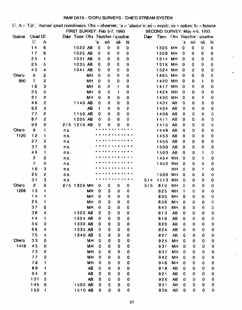
RAW DATA - 'O'OPU SURVEYS - 'OHE'O STREAM SYSTEM
U , A = 'Up', 'Across' quad coordinates; Obs = observer; 'a = 'alamo'o; n6 = nopili; na = &ea; hi = hinana FIRST SURVEY: Feb 5-7, 1993 SECOND SURVEY: May 4-6, 1993
Station Quad ID Date Time Obs Number l quadrat Dat! Time Obs Number lqudrat U A 'a n6 nii hi 'a n6 M hi 1 4 6 1 0 2 2 A B 0 0 0 0 1 3 0 5 MH 0 0 0 0 1 7 6 1 0 2 5 A B 0 0 0 0 1 3 0 9 MH 0 0 0 0 2 4 1 1 0 3 1 A B 0 0 0 0 1 3 1 4 MH 0 0 0 0 2 5 5 1 0 3 5 AB 0 0 0 0 1 3 1 8 MH 0 0 0 0 4 3 4 1 0 4 1 A B 0 0 0 0 1 3 2 4 MH 0 0 0 0
1
'Ohe'o 0 2 M H O 0 0 0 1 4 0 5 MH 0 0 0 0 990 7 2 M H O 0 0 0 1 4 2 0 MH 0 0 1 0
1 6 3 M H O 0 1 0 1 4 1 7 MH 0 0 0 0 2 5 0 M H O 0 1 0 1 4 2 4 MH 0 0 0 0 3 1 2 M H O 0 0 0 1 4 3 0 MH 0 0 2 0 4 8 2 1 1 4 0 AB 0 0 0 0 1 4 0 1 AB 0 0 0 0 6 2 3 A 6 1 0 0 2 1 4 0 4 AB 0 0 0 0 7 7 2 1 1 5 0 A B 0 0 0 0 1 4 0 8 A8 0 0 0 0 8 7 2 1 2 0 5 A B 0 0 0 0 1 4 1 1 AB 0 0 0 0 9 6 0 215 1 2 1 0 AB 0 0 0 0 1 4 1 5 AB 0 0 0 0
'Ohe'o 8 1 n.s. * * * * * * * * * * * * 1 4 4 9 A6 0 0 0 0 1120 1 2 1 n.s. * * * * * * * * 1 4 5 3 AB 0 0 0 0
2 7 2 n.s. * * * * * * * * * * * 1 4 5 6 AB 0 0 0 0 3 7 0 n.s. * * * * * * * * 1 5 0 0 A B 0 0 0 0 4 6 1 n.s. * * * * * * * * * * * * 1 5 0 3 AB 0 0 1 0 2 2 n.s. * * * * * * * * * 1 4 5 4 MH 0 0 1 0 7 0 n s . * * * * * * * * * 1 4 5 8 MH 0 0 0 0
1 6 3 n.s. * * * * * * * * * * * * M H O 0 1 0 2 5 2 n.s . * * * * * * * * * * 1 5 0 8 MH 0 0 0 0 3 1 3 n.s. * . * * * * * * * * * 5 1 4 1 5 1 3 M H 0 0 0 0
'Ohe'o 2 0 2 1 5 1 3 0 6 M H 0 0 0 0 515 8 1 9 M H 0 0 0 0 1268 1 3 1 M H O 0 0 0 8 2 5 MH 1 0 0 0
1 4 1 M H O 0 0 0 8 3 0 MH 0 0 0 0 2 5 1 M H O O 0 0 8 3 6 MH 0 0 0 0 3 7 0 MH 0 0 0 0 8 4 2 MH 0 0 0 0 3 8 4 1 3 2 0 A B 0 0 0 0 8 1 3 AB 0 0 0 0 4 4 1 1 3 2 4 A B 0 0 0 0 8 1 6 AB 0 0 0 0 5 9 0 1 3 3 0 AB 0 0 0 0 8 2 0 A6 0 0 0 0 6 6 4 1 3 3 5 A B 0 0 0 0 8 2 4 AB 0 0 0 0 7 0 4 1 3 4 0 A B 0 0 0 0 8 2 7 AB 0 0 0 0
'Ohe'o 3 3 0 MH 0 0 0 0 9 2 5 MH 0 0 0 0 1418 4 5 0 MH 0 0 0 0 9 3 1 MH 0 0 0 0
7 3 2 M H O 0 0 0 9 3 7 MH 0 0 0 0 7 7 2 MH 0 0 0 0 9 4 2 MH 0 0 0 0 7 9 1 M H O 0 0 0 9 4 6 MH 0 0 0 0 8 8 1 AB 0 0 0 0 9 1 8 AB 0 0 0 0 9 4 2 A B O 0 0 0 9 2 1 AB 0 0 0 0 1 3 1 2 A B O 0 0 0 9 2 6 AB 0 0 0 0 1 4 5 0 15OOAB 0 0 0 0 9 3 1 AB 0 0 0 0 1 5 0 1 1 5 1 0 AE 0 0 0 0 9 3 6 AB 0 0 0 0

RAW DATA - 'O'OPU SURVEYS - 'OHE'O STREAM SYSTEM
IJ, A -2 'IJp', 'Across' quad coordinates, Ohs .= observer; 'a - 'alamo'o; no -.I nopili, na - nakea, hi - hinana FIRST SURVEY: Feb 5-7, 1993 SECOND SURVEY: May 4-6, 1993
Station QuadID Dzxe Time Obs h b e r l q u a d r a t Dzl;e Time Obs Number / quadrat U A 'a nr> 6 fra 'a no n i hi
'Ohe'o 0 3 M H O 0 0 0 1 0 0 3 MH 0 0 0 0 1560 0 6 M H O 0 0 0 1 0 0 9 MH 0 0 0 0
1 0 M H O 0 0 0 1 0 1 4 MH 0 0 0 0 1 7 M H O O 0 0 1 0 1 9 MH 0 0 0 0 3 5 M H O O 0 0 1 0 2 4 MH 0 0 0 0
t 5 1 5 A B O O O O 1 0 0 2 A B 1 0 0 0 7 1 8 A B O O O O 1 0 0 6 AB 0 0 0 0 7 2 0 A B O O O O 1 0 0 9 AB 0 0 0 0 9 1 A B O O O O 1 0 1 4 AB 0 0 0 0
1 0 1 5 215 A B O O O O 1017 AB 0 0 0 0 Pipiwai 0 1 216 9 0 0 MH 0 0 0 0 1 1 3 9 M H 3 0 0 0
1900 0 3 M H 1 0 0 0 1 1 4 4 MH 1 0 0 0 7 3 M H 2 O O O MH 0 0 0 0
4 3 1 MH 2 0 0 0 1 1 5 5 M H O 0 0 0 5 3 3 9 4 5 MH 0 0 0 0 1 2 0 0 MH 0 0 0 0 7 7 2 9 2 0 A 6 2 0 0 0 1 1 3 1 AB 0 0 0 0 8 1 1 9 2 7 AB 0 0 0 0 1 1 4 0 A B 0 0 0 0 8 5 3 9 3 3 A B O 0 0 0 1 1 4 3 AB 1 0 0 0 8 7 2 9 3 7 AB 1 0 0 0 1 1 4 7 AB 1 0 0 0 9 6 1 9 4 4 A 0 1 0 0 0 1 1 5 2 AB 0 0 0 0
Pipiwai 1 1 1 0 1 7 M H 1 0 0 0 1 2 3 7 MH 0 0 0 0 2110 1 1 0 M H O 0 0 0 1 2 4 0 MH 0 0 0 0
1 1 1 M H O O 0 0 1 2 4 5 MH 1 0 0 0 1 8 0 M H O 0 0 0 1 2 5 2 MH 2 0 0 0 1 8 1 MH 5 0 0 0 1 2 5 7 M H 1 0 0 0 2 9 3 1 0 2 8 A B 1 0 0 0 1 2 3 3 AB 1 0 0 0 3 0 0 1 0 3 5 AB 1 0 0 0 1 2 3 6 A B 0 0 0 0 5 2 1 1 0 4 0 A B 2 0 0 0 1 2 4 0 AB 1 0 0 0 6 3 0 1 0 4 7 A B 0 0 0 0 1 2 4 4 A B 0 0 0 0 9 5 0 1 0 5 0 AB 0 0 0 0 1 2 4 9 A B 0 0 0 0
Pipiwai 1 5 1 1 1 3 0 M H 0 0 0 0 1 3 3 1 MH 0 0 0 0 2360 1 5 2 M H 1 0 0 0 1 3 3 5 MH 0 0 0 0
2 5 3 M H 1 0 0 0 1 3 4 0 MH 0 0 0 0 2 9 1 1 1 5 2 M H 0 0 0 0 1 3 4 5 MH 0 0 0 0 3 3 1 M H 1 0 0 0 1 3 5 0 MH 2 0 0 0 4 6 0 1 1 2 5 AB 0 0 0 0 1 3 2 5 A B 0 0 0 0 6 8 2 1 1 3 9 AB 0 0 0 0 1 3 2 9 A B 0 0 0 0 7 1 2 1 1 4 3 AB 0 0 0 0 1 3 3 2 A B 0 0 0 0 8 5 0 1 1 4 8 A6 0 0 0 0 1 3 3 5 A B 0 0 0 0 8 8 1 1 1 5 0 AB 1 0 0 0 515 1 3 3 8 AB 0 0 0 0
Palikea 1 4 M H O O 0 0 516 1 6 0 9 MH 0 0 0 0 1892 1 3 3 M H O O 0 0 1 6 1 3 MH 0 0 0 0
1 8 1 M H O 0 0 0 1 6 1 7 MH 1 0 0 0 3 9 2 h4H 0 0 0 0 1 6 2 2 MH 0 0 0 0 5 4 1 M H O 0 0 0 1 6 2 8 MH 2 0 0 0
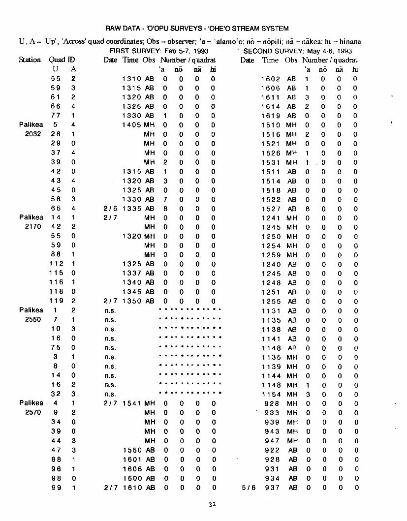
RAW DATA - 'O'OPU SURVEYS - 'OHE'O STREAM SYSTEM
U , A = 'Up', 'Across' quad coordinates; Obs = observer; 'a = 'alamo'o; no = nopili; na - niikea; hi = hinma FIRST SURVEY: Feb 5-7, 1993 SECOND SURVEY: May 4-6, 1993
Station Quad ID Date Time Obs Number / quadrat Date Time Obs Number l quadrat U A 'a n6 nii ki 'a no 6 hi 5 5 2 1310 A6 0 0 0 0 1602 AB 1 0 0 0 5 9 3 1315 AB 0 0 0 0 1606 AB 1 0 0 0 6 1 2 1 3 2 0 A B 0 0 0 0 1611 A8 3 0 0 0 6 6 4 1 3 2 5 A B 0 0 0 0 1614 AB 2 0 0 0 7 7 1 1 3 3 0 A B 1 0 0 0 1619 AB 0 0 0 0
Palikea 5 4 1 4 0 5 M H 0 0 0 0 1 5 1 0 M H O 0 0 0 *
2032 2 6 1 M H O O O 0 1516 MH 2 0 0 0 2 9 0 MH 0 0 0 0 1 5 2 1 M H O 0 0 0 3 7 4 MH 0 0 0 0 1526 MH 1 0 0 0 3 9 0 M H 2 O O O 1531 MH 1 0 0 0 4 2 0 1315 A6 1 0 0 0 1511 A6 0 0 0 0 4 3 4 1 3 2 0 A B 3 0 0 0 1514 A6 0 0 0 0 4 5 0 1325 AB 0 0 0 0 1518 A6 0 0 0 0 5 8 3 1330 AB 7 0 0 0 1522 A6 0 0 0 0 6 5 4 216 1 3 3 5 A B 8 0 0 0 1 5 2 7 A B 8 0 0 0
Palikea 1 4 1 217 M H O 0 0 0 1 2 4 1 M H O 0 0 0 2170 4 2 2 M H O 0 0 0 1245 MH 0 0 0 0
5 5 0 1320 MH 0 0 0 0 1250 MH 0 0 0 0 5 9 0 M H O O 0 0 1254 MH 0 0 0 0 8 8 1 M H O 0 0 0 1259 MH 0 0 0 0 1 1 2 1 1325 AB 0 0 0 0 1240 AB 0 0 0 0 1 1 5 0 1 3 3 7 A B 0 0 0 0 1245 A6 0 0 0 0 1 1 6 1 1340 AB 0 0 0 0 1248 AB 0 0 0 0 1 1 8 0 1 3 4 5 A B 0 0 0 0 1 2 5 1 A B 0 0 0 0 1 1 9 2 2 1 7 1 3 5 0 A B 0 0 0 0 1255 A6 0 0 0 0
Palikea 1 2 n.s. * * * * * * * * * * 1131 AB 0 0 0 0 2550 7 1 ns . * * * * * * * * * * 1135 A6 0 0 0 0
1 0 3 n.s. * * * * * * * * * 1138 AB 0 0 0 0 1 6 0 n.s. * * * * * * * * * 1141 A6 0 0 0 0 7 5 0 n.s. * * * * * * * * * * 1148 AB 0 0 0 0 3 1 n.s. * * * * * * * * * * 1 1 3 5 M H O 0 0 0 8 0 n.s. * * * * * * * * * * 1 1 3 9 M H O 0 0 0
1 4 0 n.s. * * * * * * * * * * * 1 1 4 4 M H O 0 0 0 1 6 2 n.s. * * * * * * * * * * * 1148 MH 1 0 0 0 3 2 3 n.s. * * * * * * * * * * 1 1 5 4 M H 3 0 0 0
Palikea 4 1 2 1 7 1 5 4 1 M H 0 0 0 0 928 MH 0 0 0 0 2570 9 2 M H O 0 0 0 a 9 3 3 MH 0 0 0 0
3 4 0 M H O 0 0 0 9 3 9 MH 0 0 0 0 3 9 0 M H O 0 0 0 9 4 3 MH 0 0 0 0 4 4 3 M H O O O O 947 MH 0 0 0 0 4 7 3 1550 AB 0 0 0 0 9 2 2 AB 0 0 0 0 8 8 1 1 6 0 1 A B 0 0 0 0 9 2 8 A6 0 0 0 0 9 6 1 1 6 0 6 A6 0 0 0 0 9 3 1 AB 0 0 0 0 9 8 0 1 6 0 0 A B 0 0 0 0 9 3 4 AB 0 0 0 0 9 9 1 217 1610 AB 0 0 0 0 516 9 3 7 AB 0 0 0 0

SIZE CLASSES OF 'O'OPU RECORDED
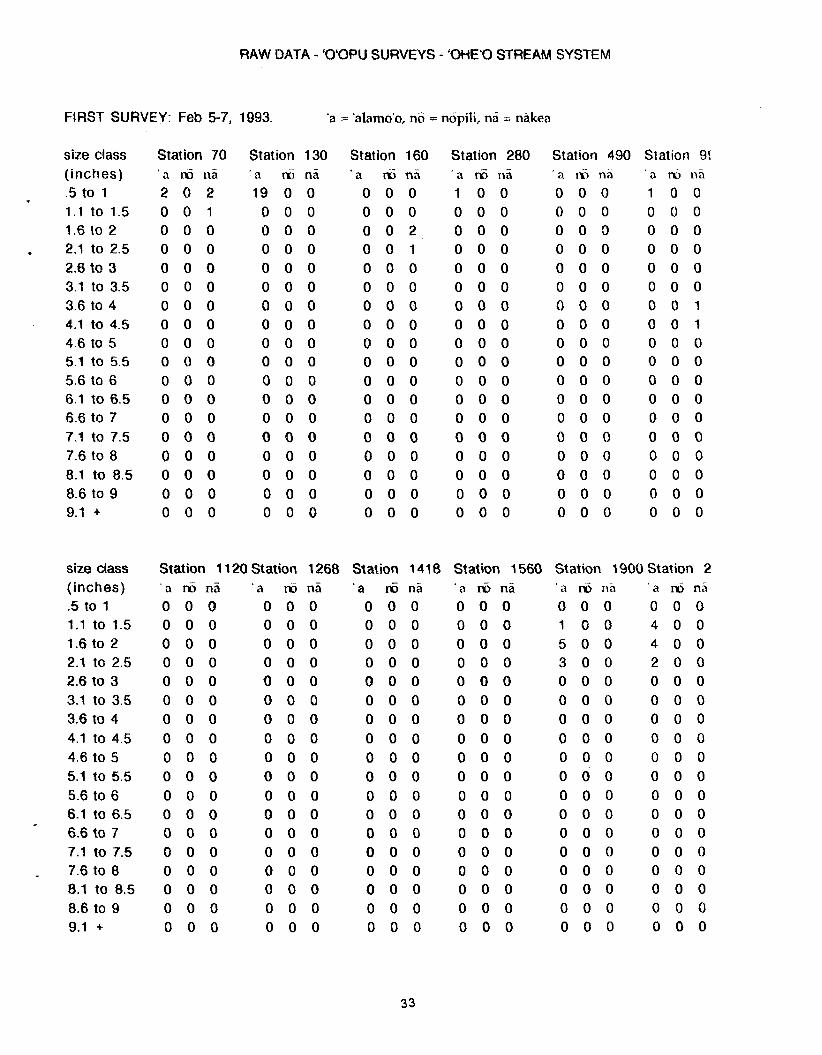
RAW DATA - 'O'OPU SURVEYS - 'OHE'O STREAM SYSTEM
FIRST SURVEY: Feb 5-7, 1993. 'a - 'alamo'o, no = nopili, n5 = nakea
size class (inches) .5 to 1 1.1 to 1.5 1.6 to 2 2.1 to 2.5 2.6 to 3 3.1 to 3.5 3.6 to 4 4.1 to 4.5 4.6 to 5 5.1 to 5.5 5.6 to 6 6.1 to 6.5 6.6 to 7 7.1 to 7.5 7.6 to 8 8.1 to 8.5 8.6 to 9 9.1 +
size class (inches) .5 to 1 1.1 to 1.5 1.6 to 2 2.1 to 2.5 2.6 to 3 3.1 to 3.5 3.6 to 4 4.1 to 4.5 4.6 to 5 5.1 to 5.5 5.6 to 6 6.1 to 6.5 6.6 to 7 7.1 to 7.5 7.6 to 8 8.1 to 8.5 8.6 to 9 9.1 +
Station 70 ' a m n5 2 0 2 0 0 1 0 0 0 0 0 0 0 0 0 0 0 0 0 0 0 0 0 0 0 0 0 0 0 0 0 0 0 0 0 0 0 0 0 0 0 0 0 0 0 0 0 0 0 0 0 0 0 0
Station ' a t-6
19 0 0 0 0 0 0 0 0 0 0 0 0 0 0 0 0 0 0 0 0 0 0 0 0 0 0 0 0 0 0 0 0 0 0 0
Station 1 120 Station 1268 ' a rii n5 ' a rb ni 0 0 0 0 0 0 0 0 0 0 0 0 0 0 0 0 0 0 0 0 0 0 0 0 0 0 0 0 0 0 0 0 0 0 0 0 0 0 0 0 0 0 0 0 0 0 0 0 0 0 0 0 0 0 0 0 0 0 0 0 0 0 0 0 0 0 0 0 0 0 0 0 0 0 0 0 0 0 0 0 0 0 0 0 0 0 0 0 0 0 0 0 0 0 0 0 0 0 0 0 0 0 0 0 0 0 0 0
Station 160 'a 6 1 1 5 0 0 0 0 0 0 0 0 2 0 0 1 0 0 0 0 0 0 0 0 0 0 0 0 0 0 0 0 0 0 0 0 0 0 0 0 0 0 0 0 0 0 0 0 0 0 0 0 0 0 0 0 0 0
Station 1418 ' a niina 0 0 0 0 0 0 0 0 0 0 0 0 0 0 0 0 0 0 0 0 0 0 0 0 0 0 0 0 0 0 0 0 0 0 0 0 0 0 0 0 0 0 0 0 0 0 0 0 0 0 0 0 0 0
Station 280 ' a 6 nii 1 0 0 0 0 0 0 0 0 0 0 0 0 0 0 0 0 0 0 0 0 0 0 0 0 0 0 0 0 0 0 0 0 0 0 0 0 0 0 0 0 0 0 0 0 0 0 0 0 0 0 0 0 0
Station 15fN ' a r i j na 0 0 0 0 0 0 0 0 0 0 0 0 0 0 0 0 0 0 0 0 0 0 0 0 0 0 0 0 0 0 0 0 0 0 0 0 0 0 0 0 0 0 0 0 0 0 0 0 0 0 0 0 0 0
Station 490 ' a r i 5 na
0 0 0 0 0 0 0 0 0 0 0 0 0 0 0 0 0 0 0 0 0 0 0 0 0 0 0 0 0 0 0 0 0 0 0 0 0 0 0 0 0 0 0 0 0 0 0 0 0 0 0 0 0 0
Station 9! a in na 1 0 0 0 0 0 0 0 0 0 0 0 0 0 0 0 0 0 0 0 1 0 0 1 0 0 0 0 0 0 0 0 0 0 0 0 0 0 0 0 0 0 0 0 0 0 0 0 0 0 0 0 0 0
Station 1900 Station 2 'a ti5 n5 ' a n5 na 0 0 0 0 0 0 1 0 0 4 0 0 5 0 0 4 0 0 3 0 0 2 0 0 0 0 0 0 0 0 0 0 0 0 0 0 0 0 0 0 0 0 0 0 0 0 0 0 0 0 0 0 0 0 0 0 0 0 0 0 0 0 0 0 0 0 0 0 0 0 0 0 0 0 0 0 0 0 0 0 0 0 0 0 0 0 0 0 0 0 0 0 0 0 0 0 0 0 0 0 0 0 0 0 0 0 0 0
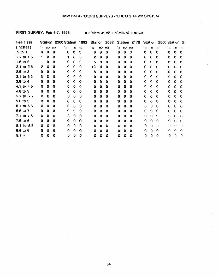
RAW DATA - 'O'OPU SURVEYS - 'OHE'Q STREAM SYSTEM
Fl RST SURVEY: Feb 5-7, 1993. 'a = 'alamo'o, ni5 = nopili, n5 = niikerr
size class (inches) .5 to 1 1.1 to 1.5 1.6 to 2 2.1 to 2.5 2.6 to 3 3.1 to 3.5 3.6 to 4 4.1 to 4.5 4.6 to 5 5.1 to 5.5 5.6 to 6 6.1 to 6.5 6.6 to 7 7.1 to 7.5 7.6 to 8 8.1 to 8.5 8.6 to 9 9.1 +
Station 2360 Station ' a r 6 n i i 'a nZi 0 0 0 0 0 1 0 0 1 0 1 0 0 0 0 2 0 0 0 0 0 0 0 0 0 0 0 0 0 0 0 0 0 0 0 0 0 0 0 0 0 0 0 0 0 0 0 0 0 0 0 0 0 0 0 0 0 0 0 0 0 0 0 0 0 0 0 0 0 0 0 0 0 0 0 0 0 0 0 0 0 0 0 0 0 0 0 0 0 0
Station ' a 6 0 0 2 0 5 0 10 0 5 0 0 0 0 0 0 0 0 0 0 0 0 0 0 0 0 0 0 0 0 0 0 0 0 0 0 0
Station 21 70 Station 2550 Station 2' 'a 16 ni ' a rb na 'a 1x1 n5
0 0 0 0 0 0 0 0 0 0 0 0 0 0 0 0 0 0 0 0 0 0 0 0 0 0 0 0 0 0 0 0 0 0 0 0 0 0 0 0 0 0 0 0 0 0 0 0 0 0 0 0 0 0 0 0 0 0 0 0 0 0 0 0 0 0 0 0 0 0 0 0 0 0 0 0 0 0 0 0 0 0 0 0 0 0 0 0 0 0 0 0 0 0 0 0 0 0 0 0 0 0 0 0 0 0 0 0 0 0 0 0 0 0 0 0 0 0 0 0 0 0 0 0 0 0 0 0 0 0 0 0 0 0 0 0 0 0 0 0 0 0 0 0 0 0 0 0 0 0 0 0 0 0 0 0 0 0 0 0 0 0

RAW DATA - 'O'OPU SURVEYS - 'OHE'O STREAM SYSTEM
SECOND SURVEY: May 4-6, 1993. . . a ialamu'o, no : nopili, nn nnkcn
size class (inches)
* -5 to 1 1.1 to 1.5 1.6 to 2 2.1 to 2.5 2.6 to 3 3.1 to 3.5 3.6 to 4 4.1 to 4.5 4.6 to 5 5.1 10 5.5 5.6 to 6 6.1 to 6.5 6.6 to 7 7.1 to 7.5 7.6 to 8 8.1 to 8.5 8.6 to 9 9.1 +
size class (inches) .5 to 1 1.1 to 1.5 1.6 to 2 2.1 to 2.5 2.6 to 3 3.1 to 3.5 3.6 to 4 4.1 to 4.5 4.6 to 5 5.1 to 5.5 5.6 to 6 6.1 to 6.5 6.6 to 7 7.1 to 7.5 7.6 to 8 0.1 to 8.5 8.6 to 9 9.1 +
Station 70 ' a rrij na 0 0 3 0 0 5 0 0 2 0 0 4 0 0 1 0 0 1 0 0 0 0 0 1 0 0 0 0 0 0 0 0 0 0 0 0 0 0 0 0 0 0 0 0 0 0 0 0 0 0 0 0 0 0
Station 130 ' a r 3 n a 13 0 2 3 1 1 0 0 0 0 0 0 0 1 0 0 0 0 0 0 0 0 0 0 0 0 0 0 0 0 0 0 0 0 0 0 0 0 0 0 0 0 0 0 0 0 0 0 0 0 0 0 0 0
Station 1 1 20 Station 1268 'a rd n5 ' a mi n5 0 0 0 1 0 0 0 0 0 0 0 0 0 0 0 0 0 0 0 0 0 0 0 0 0 0 0 0 0 0 0 0 1 0 0 0 0 0 0 0 0 0 0 0 0 0 0 0 0 0 2 0 0 0 0 0 0 0 0 0 0 0 0 0 0 0 0 0 0 0 0 0 0 0 0 0 0 0 0 0 0 0 0 0 0 0 0 0 0 0 0 0 0 0 0 0 0 0 0 0 0 0 0 0 0 0 0 0
Station 160 ' a 5 ni 3 0 0 0 0 0 0 0 0 0 0 0 0 0 1 0 0 0 0 0 0 0 0 0 0 0 0 0 0 0 0 0 0 0 0 0 0 0 0 0 0 0 0 0 0 0 0 0 0 0 0 0 0 0
Station 280 ' a 15 nc? 5 0 1 0 0 0 0 0 0 0 0 0 0 0 0 0 0 0 0 0 0 0 0 0 0 0 0 0 0 0 0 0 0 0 0 0 0 0 0 0 0 0 0 0 0 0 0 0 0 0 0 0 0 0
Station 141 8 Station 1560 'a nii nii 'a ri5 nii 0 0 0 0 0 0 0 0 0 0 0 0 0 0 0 0 0 0 0 0 0 1 0 0 0 0 0 0 0 0 0 0 0 0 0 0 0 0 0 0 0 0 0 0 0 0 0 0 0 0 0 0 0 0 0 0 0 0 0 0 0 0 0 0 0 0 0 0 0 0 0 0 0 0 0 0 0 0 0 0 0 0 0 0 0 0 0 0 0 0 0 0 0 0 0 0 0 0 0 0 0 0 0 0 0 0 0 0
Station 490 ' a nii n5 0 0 0 0 0 0 0 0 0 0 0 0 0 0 0 0 0 0 0 0 0 0 0 0 0 0 0 0 0 0 0 0 0 0 0 0 0 0 0 0 0 0 0 0 0 0 0 0 0 0 0 0 0 0
Station 990 ' a 6 nii 0 0 0 0 0 0 0 0 0 0 0 0 0 0 0 0 0 0 0 0 1 0 0 0 0 0 0 0 0 1 0 0 0 0 0 0 0 0 1 0 0 0 0 0 0 0 0 0 0 0 0 0 0 0
Station 1900 Station 21 10 ' a 6 1-15 'a ti5 n5 0 0 0 0 0 0 0 0 0 1 0 0 3 0 0 3 0 0 1 0 0 2 0 0 2 0 0 0 0 0 0 0 0 0 0 0 0 0 0 0 0 0 0 0 0 0 0 0 0 0 0 0 0 0 0 0 0 0 0 0 0 0 0 0 0 0 0 0 0 0 0 0 0 0 0 0 0 0 0 0 0 0 0 0 0 0 0 0 0 0 0 0 0 0 0 0 0 0 0 0 0 0 0 0 0 0 0 0


NUMBER OF 'OPAE RECORDED

HAW DATA - 'OPAE SURVEYS - 'OHE'O STREAM SYSTEM
U, A f: 'Up', 'Across' quad coordinates; Obs = observer; # = number 'opae!quadrar;
Station @ad I5 U A
70 0 3 70 0 4 70 1 1 70 5 1 70 7 1 70 9 2 70 10 7 70 19 5 70 25 0 70 32 4 130 0 2 130 0 7 130 1 4 130 7 5 130 16 0 130 19 0 130 25 0 130 29 0 130 31 0 130 39 0 280 5 2 280 14 1 280 16 1 280 22 0 280 25 1 280 25 3 280 31 5 280 38 3 280 47 2 280 59 2 990 0 2 990 7 2 990 16 3 990 2 5 0 990 3 1 2 990 48 2 990 62 3 990 77 2 990 8 7 2 990 9 6 0 1418 12 0 1418 19 1
FIRST SURVEY MARCH 3-21, '93 'I'irnel I>* Obs IC
tE.alm SURVEY MAY 26-29, '93 '~ ime/ Dzie Obs
0 0 Note: unless otherwise 0 indicated, all observ- 0 ations made by MH 0 0 0 0 0 0 0 0 0 0 0 0 0 0 0 0 0 0 0 0 0 0 1
0 0 0 0
0 1 1
0 0 0 1 0 0 26 28
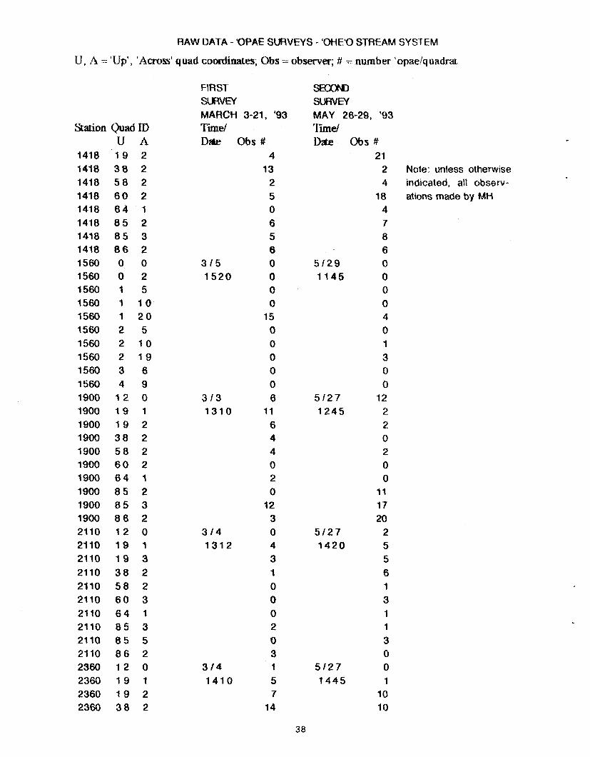
RAW DATA - OPAE SURVEYS - 'OHED STREAM SYSTEM
IJ , A - ' IJp' , 'Across:' quad coordinates; Obs = observer; # = number ' opaeiq uadm
Station Quad ID U A
1418 1 9 2 1418 38 2 1418 5 8 2 1418 6 0 2 1418 6 4 1 1418 8 5 2 1418 8 5 3 1418 8 6 2 1560 0 0 1560 0 2 1560 1 5 1560 1 1 0 1560 1 2 0 1560 2 5 1560 2 1 0 1560 2 1 9 1560 3 6 1560 4 9 1900 1 2 0 1900 1 9 1 1900 1 9 2 1900 3 8 2 1900 5 8 2 1900 6 0 2 1900 6 4 1 1900 8 5 2 1900 8 5 3 1900 8 6 2 2110 1 2 0 2110 19 1 2110 1 9 3 2110 3 8 2 2110 5 8 2 2110 6 0 3 2110 6 4 1 2110 8 5 3 2110 8 5 5 2110 8 6 2 2360 1 2 0 2360 1 9 1 2360 1 9 2 2360 3 8 2
FIRST SURVEY MARCH 3-21, '93 Time/ Dlrlte Obs #
4 13
2 5 0 6 5 6
315 0 1520 0
0 0
15 0 0 0 0 0
313 6 131 0 11
6 4 4 0 2 0
12 3
314 0 1312 4
3 1 0 0 0 2 0 3
3 1 4 1 1416 5
7 14
SEOON)
S W MAY 26-29, '93 T i Dzre Obs #
21 2 Note: unless otherwise 4 indicated, all observ-
18 ations made by MH 4 7 8 6
5 / 2 9 0 1145 0
0 0 4 0 1 3 0 0
5127 12 1245 2
2 0 2 0 0
11 17 20
5127 2 1420 5
5 6 1 3 1 1
3 0
5127 0 1445 1
10 10

RAW DATA - 'OPAE SURVEYS - 'OHE'O STREAM SYSFE-M
U, A - 'IJp' , ' A m a ' quad coodinates; C)bs observer; # = number 'upadq uadrat
%ion Quad 1D
FIRST SURVEY MARCH 3-21, '93 Timd Date Obs #
SKXIN)
eiwvEY MAY 26-29, '93 'Iimet Date CPbs
9 16 Note: unless otherwise 3 indicated, all observ- 5 at~ons made by MH 3 0 2 7 0 6 6 6 2 1
0 10 0 2 0 2 0 0 0 0 0 0 2 0 0 0 6 9 0
10 5 0 0 0 0 0 0

RAW DATA - OPAE SURVEYS - 'OHE'O STREAM S Y S E ~ V ~
U , A = 'Up', 'Across' quad coordinates; Obs = observer; # - number 'opae!quadrat
Station Quad ID U A
2170 6 4 1 2170 8 5 2 2170 8 5 3 2170 8 6 2 2550 1 2 0 2550 1 9 1 2550 1 9 2 2550 3 8 2 2550 5 8 2 2550 6 0 2 2550 6 4 1 2550 8 5 2 2550 8 5 3 2550 8 6 2 2570 1 2 0 2570 1 9 1 2570 1 9 2 2570 3 8 2 2570 5 8 2 2570 6 0 2 2570 6 4 1 2570 8 5 2 2570 8 5 3 2570 8 6 2 2770 2 0 2770 9 0 2770 9 1 2770 2 8 2 2770 3 8 2 2770 4 0 2 2770 4 4 1 2770 5 5 0 2770 5 5 2 2770 6 0 2
FIRST SURVEY MARCH 3-21, '93 Timd Date Obs #
0 3 7 0
315 16 1300 0
0 0
41 0 0 0 0 0
315 0 1130 0
0 0 0 0 0 0 0 0
315 0 930 0
0 59 0
20 0 1 0 0
SKX)ND
SWVEY MAY 26-29, '93 Tunel Date Obs #
0 0 Note: unless otherwise 1 indicated, all observ-
10 ations made by MH 5 / 2 8 47 1244 2
0 0
36 1
24 0 0 0
5 / 2 8 0 1200 0
0 0 0 0 0 0 0 0
5 12 8 8 1015 20
27 1 0 8 5 5 1
20

SIZE CLASSES OF 'OPAE RECORDED
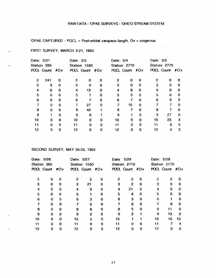
RAW DATA - 'OPAE SURVEYS - 'OHE'O STREAM SYSTEM
'OPAE CAPTURED - POCL = Post-orbital carapace length, Ov = ovigerous
FIRST SURVEY, MARCH 3-21, 1993
SECOND SURVEY, MAY 26-29, 1993
Date: 3121 Station 280 POCl hunt
Date: 315 Station 1560 POCL Count #Ov
Date: 5/28 Station 280 pax Count
Date: 5/27 Station 1560 POC1_ Count tOv
Date: 314 Station 2710 POCL Count
Date: 5129 Station 2710 POCL Count
Date: 315 Station 2770 POCt Count
Station 2770 Fax Count #Ov

NUMBER, SIZE CLASSES, AND NUMBER OF EGG CASES OF HIHIWAI RECORDED
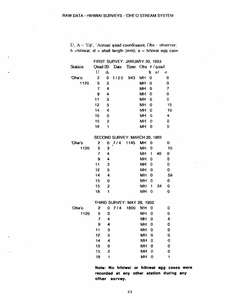
RAW DATA - HIHIWAI SURVEYS - 'OHE'O STREAM SYSTEM
U , A -- 'Up', 'Across' quad coordinates; Obs - observer; h zhihiwai; sl = shell length (rnrn); e = hihiwai egg case
FIRST SURVEY: JANUARY 20, 1993 %on Quad ID D a e Ilime Obs # /quad
U A h sl e 'Ohe'o 2 0 1/20 943 MH 0 0
1120 5 3 MH 0 0 7 4 MH 0 7 9 4 MH 0 0
11 3 MH 0 0 12 5 MH 0 15 14 4 MH 0 19 15 0 MH 0 4 15 2 MH 0 0 18 1 MH 0 0
SECOND SURVEY: MARCH 20,1993 'Ohe'o 2 0 7 / 4 1145 MH 0
1120 5 3 MH 0 7 4 MH 1 40 9 4 MH 0
11 3 MH 0 12 5 MH 0 14 4 MH 0 15 0 MH 0 15 2 MH 1 34 18 1 MH 0
THIRD SURVEY: MAY 26, 1993 'Ohe'o 2 0 714 1800 MH 0
1120 5 3 MH 0 7 4 MH 0 9 4 MH 0
11 3 MH 0 12 5 MH 0 14 4 MH 0 15 0 MH 0 15 2 MH 0
18 1 MH 0
Note: No hihiwei or hihiwai egg cases were recorded at any other station during any other survey.
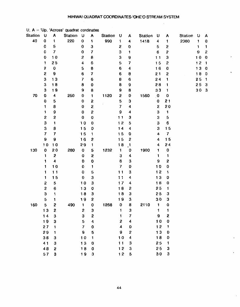
HlHlWAl QUADRAT COORDINATES-'OHE'O STREAM SYSTEM
U, A = 'Up, 'Across' quadrat cordinates Station U A Station U A Station U A
40 0 1 220 0 1 990 1 4 0 5 0 3 2 0 0 7 0 7 3 1 0 10 2 8 3 9 1 25 4 6 5 7 2 0 5 8 6 4 2 9 6 7 6 8 3 13 7 6 8 6 3 18 8 0 8 9 3 19 9 8 9 8
70 0 4 250 0 1 1120 2 0 0 5 0 2 5 3 1 8 0 2 7 4 1 9 0 2 9 4 2 2 0 0 1 1 3 3 1 10 0 12 5 3 8 15 0 1 4 4 7 7 15 1 15 0 9 9 16 2 15 2 10 10 29 1 18 pll
130 0 20 280 0 5 1232 1 0 1 2 0 2 3 4 1 4 0 0 6 3 1 10 0 1 7 0 1 1 1 0 5 1 1 3 1 15 0 3 1 1 4 2 5 10 3 17 4 2 6 13 0 18 2 3 1 18 3 18 3 5 1 19 2 19 3
160 5 2 490 1 0 1268 0 8 13 2 2 3 1 3 14 3 3 2 1 7 19 3 5 4 2 4 27 1 7 0 4 0 29 1 9 5 9 2 38 3 10 1 10 4 4 1 3 13 0 1 1 3 4 8 2 18 0 12 3 57 3 19 3 12 5
Station U A 1418 4 1
5 2 6 2 1 1 3 15 2 16 0 21 2 24 1 28 1 33 1
1560 0 0 0 21 2 20 3 1 3 5 3 6 3 15 4 7 4 15 4 24
1900 1 0 1 1 9 2 10 0 12 1
13 0 18 0 25 1 25 3 30 3
2110 1 0 1 1 9 2 10 0 1 2 1 13 0 18 0 25 1 25 3 30 3
Station U A 2360 1 0
1 1 9 2 10 0 12 1 13 0 18 0 25 1 2 5 3 30 3

NUMBER, SIZE CLASSES, AND ADDITIONAL CHARACTERISTICS OF ~ a c r o b r a c h i ~ ~ R E C O R D E D

RAW DATA - M. lar SURVEYS - 'OHE'O STREAM SYSTEM
POCL Post orb~tal carapace length (mm), Ov ovigerous; BSD presence of black-spotted dlsease symptoms ' * - time (2400 clock), date trap set and retrieved; FIRST SURVEY SECOND S U N THIRD SURVEY FOUR[H SURVEY Jan 3-5, '93 MARCH 31-April 2, '93 JULY 17-19, '93 November 20-23, '93 Station POCL Station PO(X Sex Ov Station POCL Sex Ov BSD Station POCL Sex Ov RSD

RAW DATA - M. tar SURVEYS - 'OHE'O STREAM SYSTEM
POCL - Post orbital carapace length (mm); Ov = ovigerous; BSD = presence of black-spotted disease symptoms. '* = time (2400 clock), date trap set and retrieved; FIRST SURVEY S€CONDSURVP/ Jan 3-5, '93 MARCH 31-April 2, '93 Station POCL Stdon POCX Sex Ov "1451, 3 - 0650, 4 170 46 m
220 28 CVIG E\?t ;~ i
*1345, 31 - 0749, 1 *1500, 3 - 0700, 4 220 29 f n
250 11 220 31 f n 250 17 220 46 m 250 21
'1340, 31 - 0754, 1 *1510, 3 - 0707, 4 250 23 m
280 41 250 11 250 35 f n
*1535, 3 - 0722, 4 490 45 *1341, 31 - 0759, 1
'1205, 4 - 0702, 5 1220 none cwgw
THIRD SURVEY JULY 17-19, '93 Station POCL Sex Ov BSD
70 22 m n 70 28 f y y
FOURTH SURVEY November 20-23, Station POCL Sex
130 46 m 130 47 m 130 45 m 130 42 m 130 37 m 130 34 m
'93. Ov BSD
n n
Y Y n n

RAW DATA - M. lar SURVEYS - 'OHE'O STREAM SYSTEM
POCL = Post orbital carapace length (mm); Ov = ovigerous; BSD = presence of black-spotted disease symptoms. '* = time (2400 clock), date trap set and retrieved; FIRST SURVEY SECOND SURVEY Jan 3-5, '93 MARCH 31-April 2, '93 !Station POCL Station POCL Sex Ov 1232 13 990 45 m
990 41 m *1216, 4 - 0 7 1 2 , 5 990 29 f n 1268 43 990 41 m - 1268 46 990 41 m
990 37 m *1245, 4 - 0738, 5 990 48 m 1 4 1 8 none caught 990 44 m
990 41 m *1300, 4 - 0742, 5 1502 none caught '1420, 3 1 - 0835, 1
1120 9 *1323, 4 - 0753, 5 1120 41 m 1560 33 1120 12
1120 40 m *1325, 4 - 0801, 5 1120 41 m 1570 21 1570 18 *1445, 31 - 0957, 1
1220 8 *1338, 4 - 0810, 5 1220 37 f n 1630 11 1630 20 *1545, 31 - 1002, 1
1232 41 m *1619, 4 - 1009, 5 1232 14 1892 33
*1545, 31 - 1006, 1 *1410, 4 - 0833, 5 1268 18 m 1900 34 1268 30 m 1900 50 1268 51 m
*1636, 4 - 1037, 5 *1630, 31 - 1033, 1 1904 none caught 1418 18 m
4 - 0842, 5 *1620, 31 - 1038, 1 43 1502 none caught 47 43 *1611, 31 - 1045, 1 36 L3Vll i~ao 05 1560 12
1560 48 m 4 - 1046, 5 1560 55 m
21 24 "1612, 31 - 1051, 1
1570 14 4 - 0918, 5 1570 28 f n
THIRD SURVEY JULY 17-19, '93 Station POCL Sex Ov BSD
170 34 f y n 170 45 m Y 170 26 f y n 170 31 m n
"1707, 17 - 0912, 18 530 trap exposed
FOUATH SUFNEY November 20-23, '93. &don POCL Sex Ov LED
21 - 0724, 22 none caught

RAW DATA - M. lar SURVEYS - 'OHE'O STREAM SYSTEM
POCL ; Post orbital carapace length (mm); Ov = ovigerous; BSD = presence of black-spotted disease symptoms. " - time (2400 clock), date trap set and retrieved; FIRST SURVEY SECOND SURVEY Jan 3-5, '93 MARCH 31-April 2, '93 Station POa Station F)OCL Sex Ov 2032 46 1570 55 m
*1450, 4 - 0905, 5 *1630, 31 - 1058, 1 2110 31 1630 none caught
*1700, 4 - 1100, 5 *1320, 1 2360 46 1892 low flow
trap not set i is-;?, 9 " CjY-2, 5-
2710 31 *1218, 1 - 0710, 2 2710 27 1900 47 m 2710 39 1900 31 m 2710 14 1900 30 f n
1900 47 m 1900 36 m 1900 45 m 1900 37 F n 1900 38 m
*1320, 1 1904 low flow trap not set
THIRD SURVEY JULY 17-19, '93 Station POCL Sex Ov BSD
990 39 m n 990 38 m n 990 40 m n 990 43 rn Y 990 42 m n 990 43 rn n
*1307, 18 - 0700, 19 1220 none caught
KXJmsuRVEY November 20-23, '93. Station POCL Sex Ov BSD
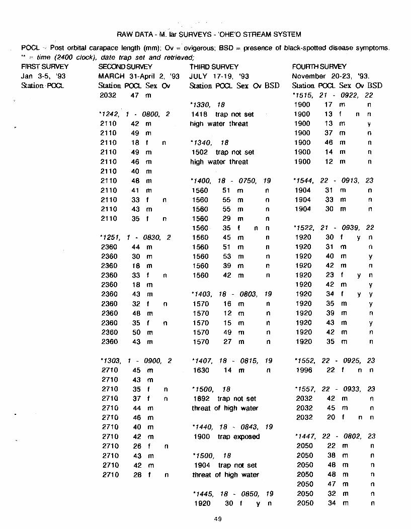
RAW DATA - M. l a SURVEYS - 'OHE'O STREAM SYSTEM
POCL = Post orbital carapace length (mm); Ov = ovigerous; BSD = presence of black-spotted disease symptoms. '* - time (2400 clock), date trap set and retrieved; FIRST SURVEY SECOND SURVEY Jan 3-5, '93 MARCH 31-April 2, '93 Station POCX Station POCL Sex Ov
2032 47 m
THIRD SURVEY JULY 17-19, '93 Station POCL Sex Ov BSD
*1330, 18 141 8 trap not set high water threat
'1340, 18 1502 trap not set high wafer threat
*1500, 18 1892 trap not set threat of high water
*1440, 18 - 0843, 19 1900 trap exposed
*1500, 18 1904 trap not set threat of high water
FOURT1-I s u m November 20-23, '93. Station POCL Sex Ov BSD *1515, 21 - 0922, 22 1900 17 rn n 1900 1 3 f n n 1900 13 m Y 1900 37 m n 1900 46 m n 1900 14 rn n 1900 1 2 m n

RAW DATA - M. lar SURVEYS - 'OHE'O STREAM SYSTEM
POCL = Post orbital carapace length (mm); Ov = ovigerous; BSD = presence of black-spotted disease symptoms. '* = time (2400 clock), date trap set and retrieved; FIRST SURVEY SECONDSUN THIRD S U R W Jan 3-5, '93 MARCH 31-April 2, '93 JULY 17-19, '93 Station POCL Station POCL Sex Ov W o n POCL Sex Ov BSD
1996 trap not set threat of high water
*1500, 18 2032 trap not set threat of high water
FOURTH SURVEY November 20-23, '93. Station POCL Sex Ov BSD 2050 27 m n 2050 32 m n 2050 29 m n 2050 37 m n 2050 29 m n 2050 37 m n 2050 37 m n 2050 47 m Y

RAW DATA - M. lar SURVEYS - 'OHE'O STREAM SYSTEM
POCL = Post orbital carapace length (mm); Ov = ovigerous; BSD - presence of black-spotted disease symptoms " time (2400 clock), date trap sot and retrieved; FIRST SURVEY SECONDSURVDl THIRD SURVEY FOURTHSURVDl . Jan 3-5, '93 MARCH 31-April 2, '93 JULY 17-19, '93 November 20-23, '93. Station POCL Station POCL Sex Ov Station POCL Sex Ov BSD Station POCL Sex Ov BSD

APPENDIX I1
RAW DATA FROM PUA'ALU'U

NUMBER OF 'O'OPU RECORDED

RAW DATA - 'O'OPU SURVEYS - PUA'ALU'U STREAM
U , A = 'Up', 'Across' quad coordinates; Obs = observer; 'a = 'alarno'o; no = nopili; na = n&ea; hi = hinana FiRST SURVEY: JULY 4, 1993 SECOND SURVEY: Oct. 5-6, 1993
Station Quad ID Date Time Obs Numberlquadrat Date T i e Obs Number /quadrat U A 'a nii n5 hi 'a no nii hi
Pua'alu'u 0 3 714 1145 MH 2 0 0 1 1016 1300 MH 2 0 0 0 70 0 4 M H 6 O O 1 M H 5 O O 1
1 1 M H 3 O O O MH 12 1 0 1 5 1 M H 1 O O O M H 3 O O O 7 1 M H 4 1 O O M H 3 O O O 9 2 M H 1 O O O M H 1 O O O
10 1 M H 1 O O O M H 1 O O O 19 2 M H 1 O O O MH 10 0 0 0 25 0 M H 5 O O 4 M H 1 O O O 32 1 M H 5 1 O O M H 6 1 O O
Pua'alu'u 0 2 7 1 4 1 3 0 0 M H 1 0 0 2 10161400 MH 7 1 0 0 130 0 3 M H 3 O O O M H 2 O O O
1 1 M H O O O O M H 6 O O 1 7 2 M H 1 O O O M H 2 O O O
16 0 M H 1 O O O M H 5 O O O 19 1 M H O O O O M H 2 O O O 25 2 M H 7 O O O M H O O O O 29 0 M H 3 O O O M H 1 O O O 31 0 M H 1 O O O M H 7 O O O 39 2 M H 5 1 O O M H 5 O O O
Pua'alu'u 5 2 714 9 3 0 M H 0 0 0 0 1015 1100 MH 9 0 0 0 $60 14 1 M H 1 O O O M H 3 O O O
16 1 M H 4 O O O M H 4 O O O 22 0 M H 8 O O O M H 2 O O O 25 1 M H O O O O M H 5 O O O 25 3 M H 1 O O O M H 5 O O O 31 5 M H 3 O O O M H 2 O O O 38 3 M H 2 O O O M H 5 O O O 47 2 M H O O O O M H O O O O 59 2 M H O O O O M H 5 O O O

RAW DATA - 'O'OPU SURVEYS - PUA'ALU'U STREAM
U, A = 'Up', 'Amss' quad coordinates; Obs = observer; 'a = 'alamo'o; no = nopili; na = niikea; hi = hinana SECOND-REPEAT SW: Oct. 67, 1993 THIRD SURVEY: Dec 4, 1993
Station Quad ID Date Time Obs Number /quadrat Date Time Obs Number l quadrat U A 'a n6 G hi 'a no na hi
Pua'alu'u 0 3 10171330 MH 6 0 1 0 1 2 1 4 1 0 4 0 P K 5 0 0 0 70 0 4 M H 5 O O O P K 1 2 0 1 0
1 1 M H 7 2 O O P K 1 O O O 5 1 3 0 0 0 P K 1 O O O 7 1 M H 2 O O O P K 3 O O O 9 2 M H 3 O O O 1048 MD 2 0 0 0
10 1 M H 3 O O O 1056 MD 4 0 0 0 19 2 M H 3 O O O 1102 MD 5 0 0 0 25 0 M H 3 1 O O 1 1 0 6 M D 6 2 0 0 32 1 M H 4 O O O 1114 MD 4 1 0 0
Pua'alu'u 0 2 1 0 1 7 1 4 3 0 M H 6 0 0 0 1 2 1 4 1 2 4 0 M D 3 0 0 0 130 0 3 M H 1 O O O 1246 MD 3 0 0 0
1 1 M H 2 O O O 1253 MD 5 0 0 0 7 2 M H 2 O O O 1 2 4 5 P K 0 0 0 0
16 0 M H 4 O O O P K O O O O 19 1 M H 2 O O O P K 6 O O O 25 2 M H 1 O O O 1250 MH 4 0 0 0 29 0 M H O O O O M H 2 O O O 31 0 M H 5 O O O M H 2 O O O 39 2 M H 5 O O O M H 3 O O O
Pua'alu'u 5 2 1 0 1 6 1 1 5 0 M H 7 0 0 0 1 2 1 4 1 4 0 0 P K 3 0 0 0 $60 14 1 M H 3 O O O 1412 PK 2 0 0 0
16 1 M H 4 O O O 1 4 2 4 P K 4 0 0 0 22 0 M H 5 O O O 1404 MD 0 0 0 0 25 1 M H 4 O O O 1 4 1 0 M D 25 0 0 0 25 3 M H 1 O O O 1414 MD 3 0 0 0 31 5 M H 1 O O O 1415 MH 2 0 0 0 38 3 M H 3 O O O M H 3 O O O 47 2 M H O O O O M H 3 O O O 59 2 M H O O O O MH 0 0 0 0

SIZE CLASSES OF 'O'OPU RECORDED

RAW DATA - 'O'OPU SURVEYS - PUA'ALU'U STREAM
'a = 'alamo'o, n6 - n6pili, nii - n6kea
FIRST SURVEY: July 4, 1993
size class (inches) .5 to 1 1.1 to 1.5 1.6 to 2 2,1 to 2.5 2.6 to 3 3.1 to 3.5 3.6 to 4 4.1 to 4.5 4.6 to 5 5.1 to 5.5 5.6 to 6 6.1 to 6.5 6.6 to 7 7.1 to 7.5 7.6 to 8 8.1 to 8.5 8.6 to 9 9.1 +
Station 70 ' a e n 5 2 0 0 5 0 0 6 0 0
1 1 1 0 3 0 0 2 0 0 0 0 0 0 0 0 0 0 0 0 1 0 0 0 0 0 0 0 0 0 0 0 0 0 0 0 0 0 0 0 0 0 0 0 0 0
Station 130 ' a m n'5 4 0 0 1 0 0 3 0 0 6 0 0 4 0 0 4 0 0
0 0 0 0 0 0 0 0 0 0 0 0 1 0 0 0 0 0 0 0 0 0 0 0 0 0 0 0 0 0 0 0 0 0 0
SECOND-REPEAT SURVEY: Oct. 6-7, 1993
size class (inches) .5 to 1 1.1 to 1.5 1.6 to 2 2.1 to 2.5 2.6 to 3 3.1 to 3.5 3.6 to 4 4.1 to 4.5 4.6 to 5
i 5.1 to 5.5 5.6 to 6 6.1 to 6.5 6.6 to 7 7.1 to 7.5 7.6 to 8 8.1 to 8.5 8.6 to 9 9.1 +
Station 70 ' a rijnii 3 0 0
11 0 0 4 0 0 16 0 0 4 0 0 1 1 0 - 0 1 0 0 0 0 0 0 0 0 0 0 0 0 0 0 0 0 0 0 1 0 0 0 0 0 0 0 0 0 0 0 0 0 0 0
Station 130 ' a m n a 2 0 0 4 0 0 9 0 0 6 0 0 7 0 0 0 0 0 0 0 0 0 0 0 0 0 0 0 0 0 0 0 0 0 0 0 0 0 0 0 0 0 0 0 0 0 0 0 0 0 0 0 0 0
Station 160 ' a * n f
1 0 0 0 0 0 0 0 0 5 0 0 6 0 0 7 0 0 0 0 0 0 0 0 0 0 0 0 0 0 0 0 0 0 0 0 0 0 0 0 0 0 0 0 0 0 0 0 0 0 0 0 0 0
Station ' a 6 0 0 4 0 7 0 12 0 5 0 0 0 0 0 0 0 0 0 0 0 0 0 0 0 0 0 0 0 0 0 0 0 0 0 0 0
SECOND SURVEY. Oct. 5-6. 1993
Station 70 ' a I$ n5 0 0 0 13 0 0 5 0 0 12 0 0 9 0 0 3 0 0 1 0 0 0 2 0 0 0 0 0 0 0 0 0 0 0 0 0 0 0 0 0 0 0 0 0 0 0 0 0 0 0 0 0 0 0
Station 130 ' a e n 5 5 0 0 3 0 0 3 0 0 9 0 0 17 1 0 0 0 0 0 0 0 0 0 0 0 0 0 0 0 0 0 0 0 O Q O 0 0 0 0 0 0 0 0 0 0 0 0 0 0 0 0 0 0
Station ' a r i i
1 0 3 0 4 0 9 0 18 0 2 0 2 0 0 0 0 0 0 0 0 0 0 0 0 0 0 0 0 0 0 0 0 0 0 0
THIRD SURVEY: Dec. 12. 1993
Station 70 'a *ni;l 10 0 0 14 1 0 4 2 0 8 0 0 7 0 0 0 0 0 0 1 0 0 0 0 0 0 0 0 0 0 0 0 0 0 0 0 0 0 0 0 0 0 0 0 0 0 0 0 0 0 0 0 0 0
Station ' a 6
2 0 13 0 12 0 1 0 0 0 0 0 0 0 0 0 0 0 0 0 0 0 0 0 0 0 0 0 0 0 0 0 0 0 0 0
Station ' a 6 11 0 14 0 11 0 6 0 3 0 0 0 0 0 0 0 0 0 0 0 0 0 0 0 0 0 0 0 0 0 0 0 0 0 0 0
NUMBER OF 'OPAE RECORDED

RAW DATA - 'OPAE SURVEYS - PUA'ALU'U STREAM
U, A = 'Up', 'Across' quad coordinates; Clbs = observer; # = number 'opae/quadrat
W o n Quad ID U A
70 0 3 0 4 1 1 5 1 7 1 9 2
10 1 19 2 25 0 32 1
130 0 2 0 3 1 1 7 2
16 0 19 1 25 2 29 0 31 0 39 2
$60 5 2 14 1 16 1 22 0 25 1 25 3 31 5 38 3 47 2 59 2
Fl RST SURVEY JULY 4, 1993. Time/ Date Obs ' # 1430 MH 4 714 MH 4
MH 0 MH 2 MH 4 MH 2 MH 0 MH 0 MH 0 MH 0
ND ND ND ND
ND ND ND ND ND ND ND ND
1515 MH 0
SKXrVD s u m Oct. 5-6, 1993. Tune/ Dace Obs ' # 1300 MH 0 1016 MH 0
MH 0 MH 4 MH 0 MH 6 MH 3 MH 7 MH 0 MH 0
1400 MH 2 1016 MH 0
MH 0 MH 0 MH 1 MH 1 MH 1 MH 2 MH 2 MH 2
1100 MH 1 1015 MH 2
MH 3 MH 0 MH 0 MH 0 MH 9 MH 5 MH 2 MH 7
SECOND-REPEAT s u m Oct. 6-7, 1993. Timd Date Obs ' # 1338 MH 0 1017 MH 0
MH 0 MH 3 MH 0 MH 7 MH 4 MH 7 MH 0 MH 0
1430 MH 2 1017 MH 2
MH 0 MH 0 MH 0 MH 4 MH 8 MH 0 MH 3 MH 7
1150 MH 4
THIRD s u m OEC.4, 1993. Tim4 D a e Obs ' # 1140 PK 0 1214 PK 0
PK 0 PK 1 PK 0 MD 4 MD 3 MD 11 MD 9 MD 0
1240 MD 3 1214 MD 25
MD 1 PK 3 PK 1 PK 0 MH 3 MH 6 MH 8 MH 1
1400 PK 4

NUMBER, SIZE CLASSES, AND NUMBER OF EGG CASES OF HiHiWAI RECORDED

RAW DATA - HlHlWAl SURVEYS - PUA'ALU'U STREAM
U , A - 'Up', 'Across' quad coordinates; Obs = observer; h =hihiwai; sl = shell length (mm); e = hihiwai egg case
FIRST SURVEY: JULY 4, 1993 SECOND SURVEY: Oct. 5-6, 1993 Station Quad ID Date Time Obs # I quad Quad ID D a e %me Obs # I quad
U A h sl e U A h sl e Pua'alu'u 4 1 7 13 1546 MH 0 0 0 3 1015 1300 MH 0 0
70 5 2 MH 0 5 0 4 MH 0 1 1 6 2 M H 1 9 0 1 1 MH 2 20,22 4
1 1 3 MH 0 0 5 1 MH 0 0 15 2 MH 0 0 7 1 MH 0 0 16 0 MH 0 6 9 2 MH 2 21,20 0 21 2 MH 1 2 2 0 10 1 MH 2 24,20 0 24 1 MH 0 4 19 2 MH 0 0 28 1 MH 0 0 25 0 MH 0 0 33 1 MH 0 0 32 1 MH 2 31,20 0
Pua'alu'u 4 1 7 14 1400 MH 0 0 0 2 1010 1400 MH 0 0 130 5 2 MH 0 0 0 3 MH 0 0
6 2 MH 0 0 1 1 MH 0 0 1 1 3 MH 0 0 7 2 MH 0 0 15 2 MH 0 0 16 0 MH 0 0 16 0 MH 0 0 19 1 MH 0 0 21 2 MH 0 0 25 2 MH 0 0 24 1 MH 0 0 29 0 MH 0 0 28 1 MH 0 0 31 0 MH 0 4 33 1 MH 0 0 39 2 MH 0 1 1
Pua'alu'u 4 1 7 / 4 1500 MH 0 0 5 2 1016 1100 MH 0 0 $60 5 2 MH 0 0 14 1 MH 0 0
6 2 MH 0 0 16 1 MH 0 0 1 1 3 MH 0 0 22 0 MH 0 0 15 2 MH 0 0 25 1 MH 0 2 16 0 MH 0 0 25 3 MH 0 0 21 2 MH 0 3 31 5 MH 0 0 24 1 MH 0 0 38 3 MH 0 0 28 1 MH 0 0 47 2 MH 0 0 33 1 MH 0 0 59 2 MH 0 0

RAW DATA - HlHlWAl SURVEYS - PUA'ALU'U STREAM
U, A = 'Up', 'Across' quad coordinates; Obs = observer; h =hihiwai; sl = shell length (mm); e = hihiwai egg case
-on Quad ID u
Pua'alu'u 0 70 0
1 5 7 9
10 19 25 32
Pua'alu'u 0 130 0
1 7
16 19 25 29 3 1 39
Pua'alu'u 5 $60 14
16 22 25 25 3 1 38 47 59
SECOND-REPEAT SURVEY: Oct. 6-7, 1993. Date Time Obs Number /quadrat
h sl e 10161330 MH 0 0
MH 1 23 0 MH 0 0 MH 0 0 MH 0 6 . MH 1 19 14
THIRD SURVEY: Dec. 4, 1993 Date Tune Obs Numberlquadrat
h sl e 1016 1300 PK 1 19 1
PK 0 0 PK 0 0 PK 0 1 PK 0 0 MD 0 13

APPENDIX I11
CODE FOR RESAMPLING PROGRAM

PROGRAM TO ESTIMATE THE NON-CENTRALITY PARAMETER FOR THE POWER OF A ONE-SAMPLE, TWO-TAILED t-TEST
REM "numberofstations" is the number of stations used during the actual survey. REM "quadnum" is the number of quadrat counts to be randomly selected from each REM station by the program from the real data recorded during the actual survey REM (i.e. the desired number of quadrats to be used in some future survey) REM "nt" is the number of trials for the simulation. REM "nsp" is the number of stations used in the calculation of the non-centrality REM parameter (i.e. the desired number of stations to be used in some REM future survey) REM "differencetodetect" is the change in population abundance desired to be detected REM Note: The first subscript of the arrays "stnBackn, "q", and "sqrdn must be REM changed manually to equal "numberofstations." REM Note: The second subscript of the arrays "qw and "sqrdn must be changed manually REM to match "quadnum." REM The data entered in statement "DATA" are the quadrat counts from REM the actual survey. REM The output of this program is five files entitled "amongstationcvubw, REM "themeansn, "thevariancesn, "thedelta", and "theamongsmean~tandardev.~ REM These files contain the unbiased coeffcient of variation for the mean counts from REM each station, the mean of the means from each station, the variance for the mean REM counts from each station, the non-centrality parameters for the mean counts REM from each station, and the standard deviation for the mean counts from each REM station, respectively.
LET numberofstations = 16 ! this is 16 for 'opae, 18 for 'o'opu LET quadnum = 2 LET nt= 30 LET nsp = 80 LET differencetodetect = .50 RANDOMIZE DIM stnBack( l6, l O), s tn ( l6 , 10) DIM q(16,8), sqrd(16,8) MAT READ stnBack DATA 0,0,0,0,0,0,0,0,0,0 ! each data line contains the series DATA 0,0,0,0,0,0,0,0,0,0 ! of quadrat counts recorded at a given station DATA 0,0,0,0,0,0,0,0,0,0 DATA 0,0,0,0,0,0,0,0,0,0 DATA 0,0,0,0,0,0,0,0,0,0 DATA 0,0,0,0,0,0,0,0,0,0 DATA 0,0,0,0,0,0,0,0,0,0 DATA 0,0,0,0,0,0,0,0,0,0 DATA 0,0,0,0,0,0,0,0,0,0 DATA 0,0,0,0,0,0,0,0,0,0 DATA 0,0,0,0,0,0,0,0,0,0 DATA 0,0,0,0,0,0,0,0,0,0 DATA 0,0,0,0,0,0,0,0,0,0 DATA 0,0,0,0,0,0,0,0,0,0 DATA 0,0,0,0,0,0,0,0,0,0 DATA 0,0,0,0,0,0,0,0,0,0
DIM wssum(l6),wsss(l6),smean(l6),wsstandardev(l6),wsvar(l6),wscv(l 6),wscvub(l6) DIM thevariances(30) DIM themeanofmeans(30)
. DIM amongstationcvub(30) DIM thedelta(30) DIM theamongsmeanstandardev(30)
- FOR t = 1 to nt FOR i = 1 to numberofstations F O R j = 1 to 10 LET stn(i, j) = stnBack(i, j) NEXT j NEXT i LET unbiasedcorrector = (1/(4'quadnum))+l FOR j = 1 to numberofstations LET y = 10
1994. Hodges. Population Monitoring. CPSUAJH.

FOR i = 1 to quadnum LET thechoice = int(yernd) + 1 LET q(j,i) = stn(j,thechoice) LET stn(j,thechoice) = stn(j,y) L E T y = y - 1 LET sqrd(j,i) = (q(j,i))A2 NEXT i NEXT j FOR k = 1 to numberofstations LET wssum(k) = 0 LET wsss(k) = 0 NEXT k FOR k = 1 to numberofstations FOR m = 1 to quadnum LET wssum(k) = wssum(k) + q(k,m) LET wsss(k) = wsss(k) + sqrd(k,m) NEXT m LET smean(k) = wssum(k) / quadnum LET blah = abs((wsss(k)-(wssum(k)/quadnum))/(quadnum-1)) LET wsstandardev(k) = sqr(blah) LET wsvar(k) = (wsstandardev(k))A2 IF smean(k) > 0 then LET wscv(k) = (wsstandardev(k)'l OO)lsmean(k) ELSE LET wscv(k) = 0 END IF LET wscvub(k) = (wscv(k))' unbiasedcorrector ! this is Sokal and Rohlf's
! (1981, p. 59) unbiased estimator of the coefficient of variation NEXT k LET unbiasedcorrectorll = (1/(4'numberofstations))+l LET sumofsqrdsmean = 0 LET sumofsmean = 0 FOR p = 1 to numberofstations LET sumofsmean = sumofsmean + smean(p) LET meanofstationmeans = sumofsmean / numberofstations LET sqrdsmean = smean(p)A2 LET sumofsqrdsmean = sumofsqrdsmean + sqrdsmean LET amongsmeanstandardev = sqr((sumofsqrdsmean- (sumofsmean~2/numberofstations))l(numberofstations-l))
! calc of standard deviation LET amongsmeanvar = amongsmeanstandardevA2 ! variance calculation IF meanofstationmeans = 0 then LET amonasmeancv = 0 - ELSE LET amongsmeancv = (amongsmeanstandardev'1OO)/meanofstationmeans ! calc for C.V.
END IF LET amongsmeancvub = amongsmeancv ' unbiasedcorrectorll
! this is Sokal and Rohlf's unbiased estimator of the ! coefficient of variation.
LET meanminusmeannought = differencetodetect'meanofstationmeans IF meanminusmeannought = 0 then LET delta = 99999 ELSE LET delta = meanminusmeannought/(amongsmeanstendardev/sqr(nsp)) END IF LET dfi = numberofstations - 1 ! this is degrees of freedom for I IF meanofstationmeans = 0 then LET I = 99999 ELSE LET I = (amongsmeanvar*dfi)/meanofstationmeans ! this is Elliott's (1971-page 40)
! index of dispersion END IF NEXT p PRINT t, delta LET amongstationcvub(t) = amongsmeancvub LET themeanofmeans(t) = meanofstationmeans LET thevariances(t) = amongsmeanvar LET thedelta(t) = delta LET theamongsmeanstandardev(t) = amongsmeanstandardev NEXT t
1994. Hodges. Population Monitoring. CPSUNH.

OPEN #1: name "amongstationcvub", create newold ERASE #1 FOR t = 1 to nt PRlNT #1: amongstationcvub(t) PRlNT #1 NEXT t OPEN #2: name "themeans", create newold ERASE #2 FOR t = 1 to nt PRlNT #2: themeanofmeans(t) PRlNT #2 NEXT t OPEN #3: name "thevariances", create newold ERASE #3 FOR t = 1 to nt PRlNT #3: thevariances(t) PRlNT #3 NEXT t OPEN #4: name "thedelta", create newold ERASE #4 FOR t = 1 to nt PRlNT #4: thedelta(t) PRlNT #4 NEXT t OPEN #5: name "theamongsmeanstandardev", create newold ERASE #5 FOR t = 1 to nt PRlNT #5: theamongsmeanstandardev(t) PRlNT #5 NEXT t a0
1994. Hodges. Population Monitoring. CPSUAJH.