technical note|a robust perspective on transaction costs
TRANSCRIPT
OPERATIONS RESEARCHVol. 00, No. 0, Xxxxx 0000, pp. 000–000issn 0030-364X |eissn 1526-5463 |00 |0000 |0001
INFORMSdoi 10.1287/xxxx.0000.0000
c© 0000 INFORMS
Technical Note—A Robust Perspective onTransaction Costs in Portfolio Optimization
Alba V. Olivares-NadalStatistics and Operations Research, University Pablo de Olavide (Spain), [email protected]
Victor DeMiguelManagement Science and Operations, London Business School (UK), [email protected]
We prove that the portfolio problem with transaction costs is equivalent to three different problems designed
to alleviate the impact of estimation error: a robust portfolio optimization problem, a regularized regression
problem, and a Bayesian portfolio problem. Motivated by these results, we propose a data-driven approach
to portfolio optimization that tackles transaction costs and estimation error simultaneously by treating
the transaction costs as a regularization term to be calibrated. Our empirical results demonstrate that the
data-driven portfolios perform favorably because they strike an optimal trade-off between rebalancing the
portfolio to capture the information in recent historical return data, and avoiding the large transaction costs
and impact of estimation error associated with excessive trading.
Key words : transaction costs; estimation error; robust optimization.
1. Introduction
Markowitz (1952) showed that an investor who cares only about the mean and variance of portfolio
returns should choose a portfolio on the efficient frontier. Mean-variance portfolios continue to be
the workhorse of much of the investment management industry, but two crucial aspects in their
successful implementation are estimation error and transaction costs. Estimation error is important
because to implement the mean-variance portfolios in practice one has to estimate the mean and
the covariance matrix of asset returns, and it is well known that the resulting portfolios often
perform poorly out of sample; see Michaud (1989), Chopra and Ziemba (1993), and DeMiguel
et al. (2009b). A popular approach to alleviate the impact of estimation error is to use robust
portfolio optimization; see, for instance, Goldfarb and Iyengar (2003), Garlappi et al. (2007), and
Lu (2011a,b). This approach captures the uncertainty about the mean and covariance matrix of
asset returns by assuming they may lie anywhere inside the so-called uncertainty sets. The robust
portfolio is the one that maximizes the mean-variance utility with respect to the worst-case mean
and covariance matrix of asset returns.
1

Olivares-Nadal and DeMiguel: A Robust Perspective on Transaction Costs in Portfolio Optimization2 Operations Research 00(0), pp. 000–000, c© 0000 INFORMS
Transaction costs are important because they can easily erode the gains from a trading strategy.
Transaction costs can be generally modelled with the p-norm of the portfolio trade vector. For
small trades, which do not impact the market price, the transaction cost is generally assumed to be
proportional to the amount traded, and thus it can be approximated by the 1-norm of the portfolio
trade vector. For larger trades, the literature has traditionally assumed that they have a linear
impact on the market price, and thus they result in quadratic transaction costs that are captured
by the 2-norm. Finally, several authors have recently argued that market impact costs grow as the
square root of the amount traded (Almgren et al. 2005, Frazzini et al. 2015), and thus they are
captured by the p-norm with p= 1.5.
We make a theoretical contribution and an empirical contribution. Theoretically, we show that
the portfolio optimization problem with p-norm transaction costs can be equivalently reformulated
as three different problems designed to alleviate the impact of estimation error: (i) a robust portfolio
optimization problem, (ii) a regularized regression problem, and (iii) a Bayesian portfolio problem.
These results demonstrate that incorporating a p-norm transaction cost term in the mean-variance
portfolio problem may help to reduce the impact of estimation error. This observation motivates
our empirical contribution: we propose a data-driven approach to portfolio selection that consists of
using cross-validation to calibrate the transaction cost parameter from historical data and compute
portfolios that perform well in a realistic scenario with both estimation error and transaction costs.
From a real-world perspective, combating estimation error by calibrating the transaction cost term
has two advantages over the use of robust approaches. First, practitioners are used to incorporating
transaction costs in their portfolio selection frameworks, and thus it may be easier for them to
simply calibrate the transaction cost term instead of using a more sophisticated approach based
on uncertainty sets. Second, a transaction cost term has a natural economic interpretation, and
this facilitates the task of selecting a reasonable range of parameters to calibrate from.
We compare the out-of-sample performance of the proposed data-driven portfolios on five empir-
ical datasets with that of the mean-variance portfolios that ignore transaction costs as well as
mean-variance portfolios that capture the nominal proportional transaction costs. We find that
the proposed data-driven portfolios outperform the traditional portfolios in terms of their out-
of-sample Sharpe ratio net of transaction costs. The data-driven portfolios perform well because
they calibrate the transaction cost parameter to achieve intermediate levels of turnover that strike
an optimal (data-driven) trade-off between two goals: (i) rebalancing the portfolio to capture the
information in recent historical return data, and (ii) avoiding the large transaction costs and impact
of estimation error associated with excessive trading.
The remainder of this manuscript is organized as follows. Section 2 gives our theoretical results
connecting transaction costs and robustness. Section 3 describes the proposed data-driven approach

Olivares-Nadal and DeMiguel: A Robust Perspective on Transaction Costs in Portfolio OptimizationOperations Research 00(0), pp. 000–000, c© 0000 INFORMS 3
and evaluates its out-of-sample performance. The Online Companion contains two appendices:
Appendix A with the proofs of all results and Appendix B with supplementary tables and figures.
2. Transaction costs and robustness
We consider the following mean-variance problem with p-norm transaction costs:
minw
γ
2wTΣw−µTw+κ‖Λ(w−w0)‖pp (1)
s.t. wT1N = 1,
where γ ∈R is the risk-aversion parameter, w ∈RN is the portfolio weight vector, Σ∈RN×N is the
estimated covariance matrix of asset returns, µ∈RN is the estimated mean of asset returns, κ∈R
is the transaction cost parameter, Λ ∈ RN×N is the transaction cost matrix, which we assume to
be nonsingular, w0 ∈RN is the starting portfolio, ‖s‖p is the p-norm of vector s, ‖s‖pp =∑N
i=1 |si|p,
1N ∈ RN is the vector of ones, and the constraint wT1N = 1 requires that the portfolio weights
sum up to one.
The first two terms in the objective function capture the risk-return trade-off: the first term
is the portfolio return variance scaled by the risk-aversion parameter (γ2wTΣw) and the second
term is the portfolio return mean (µTw). More importantly for our purposes, the third term in
the objective function is the p-norm transaction cost term, κ‖Λ(w−w0)‖pp. Note that we allow for
the portfolio trade vector (w−w0) to be transformed via a nonsingular transaction cost matrix Λ
before computing the p-norm.
We now introduce some basic definitions and facts. For a given vector norm ‖ · ‖, its dual norm
‖ · ‖∗ is ‖x‖∗ = max‖y‖≤1 yTx. It is easy to show that the dual norm of the p-norm is the q-norm,
where 1/p+ 1/q= 1; see Higham (2002, Section 6.1). Let Λ be a nonsingular matrix, we define the
(p,Λ)-norm of vector x as ‖x‖p,Λ := ‖Λx‖p. It is also easy to show that ‖ · ‖p,Λ is indeed a vector
norm and ‖ · ‖q,Λ−T is its dual norm.
The following proposition gives our main results.
Proposition 1. For every risk-aversion parameter γ > 0 and transaction cost parameter κ ≥ 0,
there exist δ,κ′ ≥ 0, α > 0 and µ0 such that the mean-variance problem with p-norm transaction
costs, Problem (1), is equivalent to:
(i) a robust portfolio problem:
minw
γ
2wTΣw−µTw+ max
µ∈U(δ)(µ− µ)T (w−w0), (2)
s.t. wT1N = 1,
where the uncertainty set for mean asset returns is U(δ) = {µ : ‖µ− µ‖q,Λ−T ≤ δ},
Olivares-Nadal and DeMiguel: A Robust Perspective on Transaction Costs in Portfolio Optimization4 Operations Research 00(0), pp. 000–000, c© 0000 INFORMS
(ii) a regularized linear regression problem:
minw
‖1T −Rw‖22 +κ′‖Λ(w−w0)‖pp, (3)
s.t wTµ= µ0,
wT1N = 1,
where R ∈ RT×N is the matrix whose columns contain the historical returns for each of the N
assets,
(iii) a Bayesian portfolio problem, where the investor believes a priori that the variance of the
mean-variance portfolio return has an independent distribution π(σ2), that asset returns are nor-
mally distributed, and that the mean-variance portfolio weights are jointly distributed as an Multi-
variate Exponential Power distribution, with probability density function:
π(w) =pN |Λ|
2NαNΓ(1/p)Ne−‖Λ(w−w0)‖pp
αp , (4)
where α is the scale parameter and Γ(·) is the gamma function.
A few comments are in order. Proposition 1(i) shows that the portfolio optimization problem
with p-norm transaction costs is equivalent to a robust portfolio optimization problem where the
mean of asset returns can take any value in an uncertainty set defined by the q-norm, where
1/p+ 1/q= 1. For instance, a mean-variance portfolio problem with proportional transaction costs
can be equivalently rewritten as a robust portfolio optimization problem where the mean can
take any value in an uncertainty set defined by a box centered at the nominal mean return. This
theoretical result provides theoretical justification for the well-known empirical observation that
robust portfolio policies often result in low turnover; see Fabozzi et al. (2007). Essentially, solving
a robust portfolio optimization problem is equivalent to introducing a transaction cost on any
trades. Therefore, in addition to alleviating the impact of estimation error, robustifying a portfolio
optimization problem is also likely to reduce portfolio turnover.
Proposition 1(i) also provides compelling statistical motivation for the use of quadratic trans-
action cost terms to combat estimation error. To see this, note that the portfolio problem with
quadratic transaction costs for the case with Λ = Σ1/2, which Garleanu and Pedersen (2013) argue
is realistic, is equivalent to a robust portfolio problem with ellipsoidal uncertainty set for mean
returns given by ‖µ − µ‖2,Σ−1/2 ≤ δ. Reassuringly, this ellipsoidal uncertainty set actually coin-
cides with the statistical confidence region for the sample estimator of mean returns under the
assumption that returns are independent and identically distributed as a Normal distribution with
covariance matrix Σ; see Goldfarb and Iyengar (2003).

Olivares-Nadal and DeMiguel: A Robust Perspective on Transaction Costs in Portfolio OptimizationOperations Research 00(0), pp. 000–000, c© 0000 INFORMS 5
In addition, Proposition 1(i) shows that the p-norm transaction cost can be interpreted as the
maximum regret the investor may experience (in terms of expected return) by trading from the
starting portfolio w0 to portfolio w, assuming the true mean belongs to the uncertainty set U(δ),
which is defined in terms of the dual q-norm. To see this, note that Proposition 1(i) essentially
shows that the transaction cost term can be rewritten as
κ‖Λ(w−w0)‖pp = κ‖w−w0‖pp,Λ = maxµ:‖µ−µ‖
q,Λ−T ≤δ(µ− µ)T (w−w0),
where µ is the estimated mean asset return vector, and µ is the worst-case mean asset return vector
for the given portfolio w.
Proposition 1(ii) shows that the portfolio optimization problem with p-norm transaction costs
is equivalent to a robust regression formulation of the mean-variance problem. It is well known
that the mean-variance portfolio optimization problem can be equivalently reformulated as a linear
regression problem; see, for instance, Britten-Jones (1999). We extend this result by showing that
the transaction cost term κ′‖w−w0‖pp in a mean-variance portfolio can be interpreted as a regu-
larization term that reduces the impact of estimation error on the linear regression. In particular,
for p = 1 this transaction cost term resembles a lasso regularization term, and for p = 2 a ridge
regularization term; see (James et al. 2013, Chapter 6) for a discussion of regularization techniques
in linear regression.
Proposition 1(iii) shows that the portfolio optimization problem with p-norm transaction costs
is equivalent to a Bayesian portfolio problem where the investor has a prior belief over the portfolio
weights. This result generalizes the results by DeMiguel et al. (2009a), who provide a Bayesian
interpretation for the 1-norm, 2-norm and A-norm constrained portfolios. We extend their result
to the portfolio problem with (p,Λ)-norm transaction cost, with p ∈ [1,2], by defining a new dis-
tribution, which we term the Multivariate Exponential Power (MEP) distribution. The MEP prior
distribution includes as particular cases the Multivariate Normal prior distribution for p= 2 and
Λ = Σ1/2, which corresponds to the quadratic transaction cost of Garleanu and Pedersen (2013),
and the Laplace prior distribution for p = 1 and Λ = I, where I is the identity matrix, which
corresponds to proportional transaction costs.
Finally, it is easy to see that all three parts of Proposition 1 also hold for the case where there are
additional constraints to the mean-variance problem with p-norm transaction costs by just adding
these constraints to the robust portfolio problem, the regularized linear regression problem, and
the Bayesian portfolio problem.

Olivares-Nadal and DeMiguel: A Robust Perspective on Transaction Costs in Portfolio Optimization6 Operations Research 00(0), pp. 000–000, c© 0000 INFORMS
3. Data-driven portfolios
We now propose a data-driven approach to portfolio selection that consists of treating the trans-
action cost term as a regularization term, and using cross validation to calibrate the transaction
cost parameter κ of Problem (1) as if it were the penalty parameter in a regularization term.
We assume the investor faces proportional transaction costs of 50 basis points, an assumption
that is consistent with the existing literature; see Balduzzi and Lynch (1999). We compare the
out-of-sample performance of the data-driven portfolios with that of the portfolios that ignore
transaction costs, and the portfolios that consider the nominal proportional transaction costs of
50 basis points.1
We consider five empirical datasets with US stock monthly return data, similar to those used
in the literature; see DeMiguel et al. (2009a). Specifically, we consider four datasets downloaded
from Ken French’s website, covering the period from July 1963 to December 2013: the 10 industry-
portfolio dataset (10Ind), the 48 industry-portfolio dataset (48Ind), the six portfolios of stock
sorted by size and book-to-market (6FF), and the 25 portfolios of firms sorted by size and book-to-
market (25FF). Finally, we consider a dataset with returns on individual stocks downloaded from
the CRSP database covering the period from April 1968 to April 2005. This dataset is constructed
as in DeMiguel et al. (2009a): in April of each year we randomly select 25 assets among all assets
in the CRSP dataset for which there is return data for the previous 120 months as well as for
the next 12 months. These randomly selected 25 assets become our asset universe for the next 12
months period.2
3.1. Description of the portfolios
We compare the performance of four different types of portfolios defined in terms of how they cap-
ture transaction costs. First, portfolios that ignore transaction costs, which are computed by solving
Problem (1) with transaction cost parameter κ= 0. Second, portfolios that capture the nominal
proportional transaction costs of 50 basis points, which are computed by solving Problem (1) with
κ= 0.005, p= 1, and Λ = I; that is, with transaction cost term 0.005‖∆w‖1, where ∆w =w−w0.
Finally, portfolios with calibrated transaction costs, which are computed by solving Problem (1)
with transaction cost (or penalty) parameter κ= κcv calibrated with 10-fold cross-validation, which
we explain in detail later. We consider two types of calibrated transaction costs. First, propor-
tional transaction costs (p = 1, Λ = I), which result in a transaction cost term κcv‖∆w‖1, and
1 Note that all portfolio policies are evaluated in terms of their out-of-sample returns net of the nominal propor-tional transaction costs of 50 basis points, even though the data-driven portfolios are computed using a calibratedproportional or quadratic transaction cost term.
2 We have also considered the cases with N = 50 and N = 100 stocks and we find that the relative performance of thedifferent portfolios is robust to changing the number of CRSP stocks.

Olivares-Nadal and DeMiguel: A Robust Perspective on Transaction Costs in Portfolio OptimizationOperations Research 00(0), pp. 000–000, c© 0000 INFORMS 7
second, quadratic transaction costs (p = 2, Λ = Σ1/2), which result in a transaction cost term
κcv‖Σ1/2∆w‖22. For each of these four different types of transaction costs, we compute four dif-
ferent portfolios: minimum-variance portfolio, shortsale-constrained minimum-variance portfolio,
mean-variance portfolio, and shortsale-constrained mean-variance portfolio.
A few comments are in order. First, why consider data-driven portfolios with calibrated quadratic
transaction costs when the nominal transaction costs are proportional? The answer is the data-
driven portfolios are designed to address not only transaction costs, but also estimation error, and
Section 2 argues that a quadratic transaction cost term is well suited to address estimation error.
Second, note that the penalties κcv corresponding to the data-driven portfolios with proportional
versus quadratic costs are not easy to compare. Fortunately, the data-driven portfolios with pro-
portional transaction costs can be equivalently calibrated in terms of trading volume or turnover,
‖w −w0‖1 ≤ τ . Moreover, Kourtis (2015) shows that the optimal portfolio for a mean-variance
investor with quadratic transaction costs is a convex combination of the starting portfolio and the
mean-variance portfolio in the absence of transaction costs. Consequently, for these portfolios one
can also calibrate the trading volume τ instead of the transaction cost parameter κ. Summarizing,
to facilitate the comparison between the two types of data-driven portfolios (with proportional and
quadratic costs), we calibrate these portfolios by selecting their trading volume.3
Third, we calibrate the data-driven portfolios using the bootstrap methodology of 10-fold cross-
validation; Efron and Gong (1983). Specifically, we divide the estimation window of M returns
into ten intervals of M/10 returns each. For j from 1 to 10, we remove the jth-interval from the
estimation window, and use the remaining sample returns to compute the data-driven portfolio for
each value of the trading volume τ from 0%, 0.5%, 1%, 2.5%, 5% and 10%. We then evaluate the
return of the resulting portfolios (net of transaction costs of 50 basis points) on the jth-interval.
After completing this process for each of the 10 intervals, we have the M “out-of-sample” portfolio
returns for each value of τ . Finally, we compute the variance of these out-of-sample returns and
select the value of τ that corresponds to the portfolio with smallest variance.4
3.2. Out-of-sample performance
We use a rolling-horizon methodology similar to that used in DeMiguel et al. (2009b) and DeMiguel
et al. (2009a) to compare the performance of the different portfolios. We use an estimation window
3 Kourtis’ observation applies only to the unconstrained mean-variance portfolio. For computational convenience,however, we also approximate the shortsale-constrained mean-variance and the shortsale-constrained and uncon-strained minimum-variance data-driven portfolios with quadratic transaction costs by taking a convex combinationof the starting portfolio and the target portfolio in the absence of transaction costs.
4 We have also tried using the Sharpe ratio of returns net of transaction costs as the calibration criterion. In addition,we have used 10-fold cross-validation and generalized cross-validation as defined by Fu (1998, Section 5) to calibratesimultaneously the transaction cost parameter (κ) and the type of transaction cost (proportional or quadratic).However, we find that the results are qualitatively similar, and thus we do not report them to conserve space.

Olivares-Nadal and DeMiguel: A Robust Perspective on Transaction Costs in Portfolio Optimization8 Operations Research 00(0), pp. 000–000, c© 0000 INFORMS
of M = 120 monthly returns. To test the statistical significance of the differences between the out-
of-sample Sharpe ratio of the different portfolios with those of the minimum-variance portfolio that
ignores transaction costs, we use the bootstrap methodology employed by DeMiguel et al. (2009a),
which is based on the work by Ledoit and Wolf (2008).
Strategy 10Ind 48Ind 6FF 25FF CRSP
Panel A. Portfolios that ignore transaction costs, κ= 0
Minimum-variance, shortsale unconstrained 0.3007 0.1167 0.3480 0.3124 0.3781
Minimum-variance, shortsale constrained 0.2953 0.2452* 0.2493* 0.2390** 0.3974
Mean-variance, shortsale unconstrained 0.0686* −0.0890* 0.2142* −0.0076* −0.0091*
Mean-variance, shortsale constrained 0.2128** 0.1782 0.2502* 0.2382*** 0.2194**
Panel B. Portfolios with nominal transaction costs, 0.005‖∆w‖1
Minimum-variance, shortsale unconstrained 0.2959 0.0955 0.3026** 0.3063 0.3987
Minimum-variance, shortsale constrained 0.2420*** 0.2601* 0.2374* 0.2318** 0.3925
Mean-variance, shortsale unconstrained 0.2074** −0.0523* 0.2631** −0.0467* 0.1005*
Mean-variance, shortsale constrained 0.2214** 0.2018** 0.2505* 0.2588 0.2681
Panel C. Data-driven portfolios with calibrated proportional transaction costs, κcv‖∆w‖1
Minimum-variance, shortsale unconstrained 0.3281*** 0.1505 0.3284 0.3745** 0.3977
Minimum-variance, shortsale constrained 0.3006 0.2925* 0.2479* 0.2563*** 0.3929
Mean-variance, shortsale unconstrained 0.2443 0.0039** 0.2436** −0.0442* 0.1161*
Mean-variance, shortsale constrained 0.2693 0.2248** 0.2477* 0.2442*** 0.2613***
Panel D. Data-driven portfolios with calibrated quadratic transaction costs, κcv‖Σ1/2∆w‖22
Minimum-variance, shortsale unconstrained 0.3234*** 0.2349* 0.3481 0.3761* 0.3995
Minimum-variance, shortsale constrained 0.2983 0.2762* 0.2446* 0.2460*** 0.3930
Mean-variance, shortsale unconstrained 0.2565 0.0105*** 0.2424** 0.0464* 0.1193*
Mean-variance, shortsale constrained 0.2748 0.2561* 0.2497* 0.2514*** 0.2579***
Table 1 Sharpe ratios
This table reports the monthly out-of-sample Sharpe ratio and the corresponding p-value that the Sharpe ratio
for each of the portfolios is different from that for the minimum-variance portfolio. We assign three/two/one
asterisks (*) to those portfolios whose p-values, indicating whether the differences with the benchmark minimum-
variance portfolio are significant, are lower than 0.01/0.05/0.1, respectively. The highest Sharpe ratio for each
dataset is highlighted in bold face.
Table 1 reports the out-of-sample Sharpe ratio for each of the 16 portfolio policies considered.
Panel A reports the Sharpe ratios for the portfolios that ignore transaction costs. This panel shows
that minimum-variance portfolios generally outperform mean-variance portfolios. This is explained
by the well-known difficulties associated with estimating mean returns from historical data. Impos-
ing shortsale constraints on the minimum-variance portfolio helps only for two of the datasets with
Olivares-Nadal and DeMiguel: A Robust Perspective on Transaction Costs in Portfolio OptimizationOperations Research 00(0), pp. 000–000, c© 0000 INFORMS 9
largest number of assets (48Ind and CRSP). This makes sense as estimating the covariance matrix
of asset returns is harder for datasets with many assets, and under these circumstances the short-
sale constraints will help to alleviate the impact of estimation error. Imposing shortsale constraints
on the mean-variance portfolio helps for every dataset because the unconstrained mean-variance
portfolio is very sensitive to estimation error.5
Panel B shows that capturing nominal proportional transaction costs of 50 basis points generally
helps to improve the performance of the mean-variance portfolios, but it only helps to improve the
minimum-variance portfolio for the CRSP dataset in the shortsale-unconstrained case and the 25FF
in the shortsale-constrained case. The reason for this is that the nominal transaction cost term helps
to combat estimation error to a certain extent, and this is helpful for mean-variance portfolios,
which are very sensitive to estimation error. Minimum-variance portfolios, on the other hand, are
more resilient to estimation error, and a nominal transaction cost parameter is too conservative
to strike the right balance between estimation error and transaction costs. This seems to indicate
that using a data-driven approach to calibrate the transaction cost (or penalty) parameter may
help to improve the performance.
We conclude that the shortsale-unconstrained minimum-variance portfolio that ignores transac-
tion costs is the best of the portfolios in Panels A and B and thus we consider it as the benchmark
portfolio for the data-driven portfolios in Panels C and D.
Panel C shows that the data-driven approach based on proportional transaction costs gener-
ally helps to improve the performance of the traditional portfolios. Specifically, the data-driven
shortsale-unconstrained minimum-variance portfolio outperforms the benchmark portfolio for every
dataset except 6FF, with an improvement in Sharpe ratio that ranges from 5% to 29% for the
different datasets, and is statistically significant for two of the five datasets.
Panel D shows that the data-driven approach based on quadratic transaction costs also helps
to improve the performance of the traditional portfolios. Specifically, the data-driven shortsale-
unconstrained minimum-variance portfolio with calibrated quadratic transaction costs outperforms
the benchmark portfolio for every dataset except 6FF, with an improvement in Sharpe ratio that
ranges from 5% to 101%, and is statistically significant for three out of five datasets.6
5 This is illustrated by Figure 1 in Appendix B of the Online Companion, which shows the out-of-sample monthlyreturns of the different types of shortsale-unconstrained mean-variance portfolios and shortsale-constrained mean-variance portfolios. While the shortsale-unconstrained mean-variance portfolios are very sensitive to estimation errorand consequently their returns may be quite extreme in some months, the shortsale-constrained mean-variance port-folios are more resilient to estimation error and thus result in more stable out-of-sample returns.
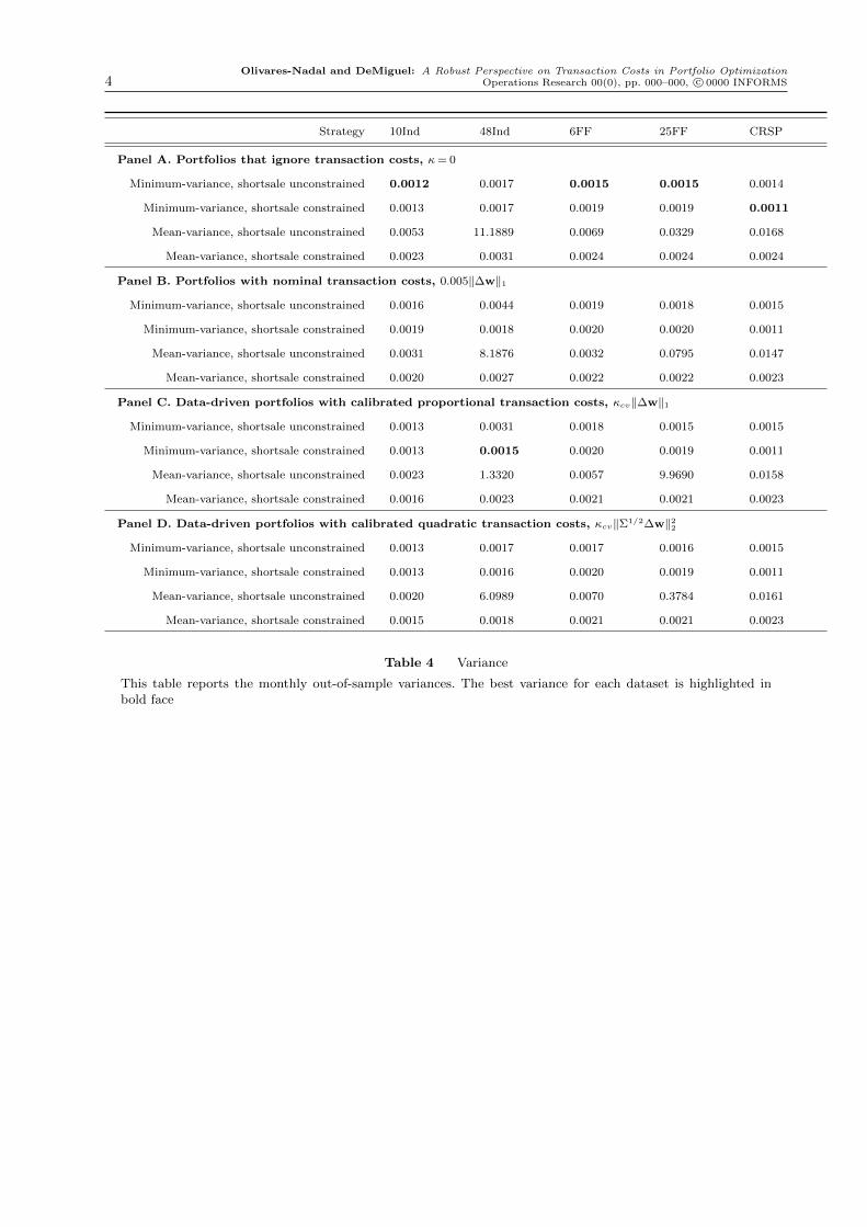
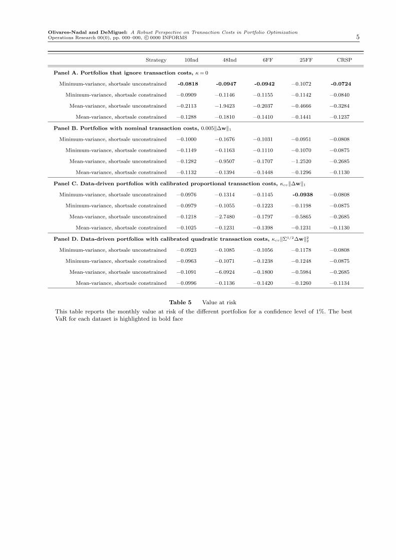
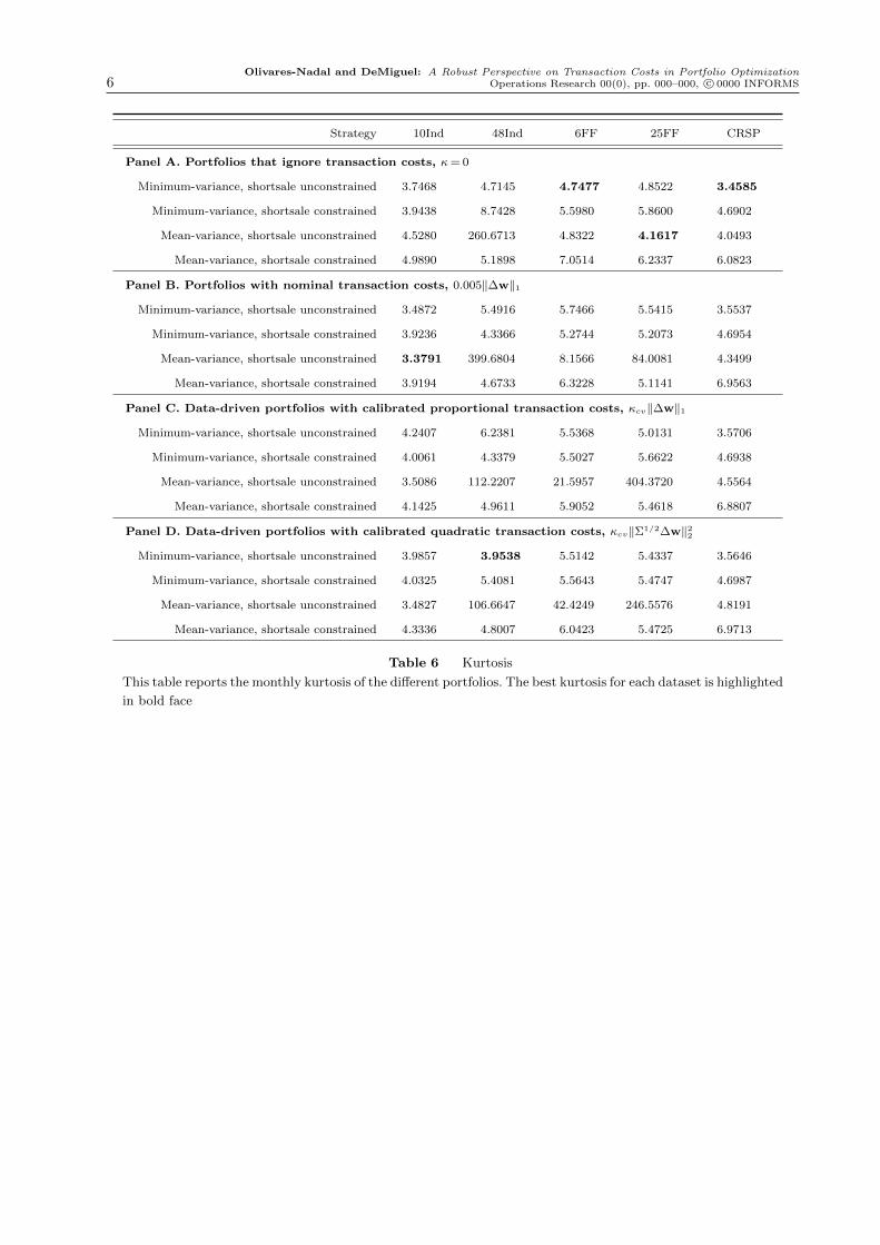
6 From the out-of-sample mean and variance for the different portfolios, reported in Tables 3 and 4 of Appendix B inthe Online Companion, we observe that considering transaction costs generally does not help to reduce the varianceof portfolio returns, but it helps to increase the mean. Thus the gains from using the proposed data-driven approachesare obtained from improvements in out-of-sample means, rather than variances. Moreover, from Tables 5 and 6 ofAppendix B in the Online Companion, we find that the relative performance of the different portfolios in terms of tailrisk as measured by value at risk and kurtosis is similar to that in terms of standard risk as measured by variance.
Olivares-Nadal and DeMiguel: A Robust Perspective on Transaction Costs in Portfolio Optimization10 Operations Research 00(0), pp. 000–000, c© 0000 INFORMS
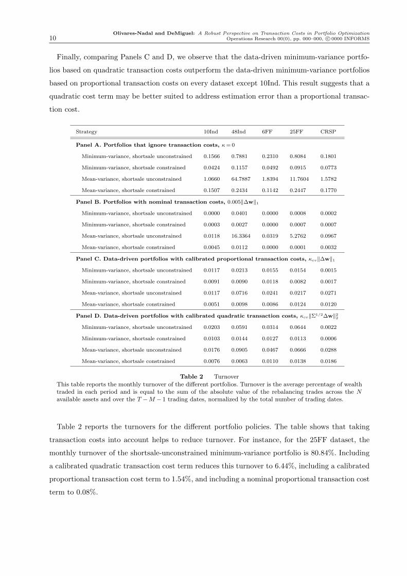
Finally, comparing Panels C and D, we observe that the data-driven minimum-variance portfo-
lios based on quadratic transaction costs outperform the data-driven minimum-variance portfolios
based on proportional transaction costs on every dataset except 10Ind. This result suggests that a
quadratic cost term may be better suited to address estimation error than a proportional transac-
tion cost.
Strategy 10Ind 48Ind 6FF 25FF CRSP
Panel A. Portfolios that ignore transaction costs, κ= 0
Minimum-variance, shortsale unconstrained 0.1566 0.7881 0.2310 0.8084 0.1801
Minimum-variance, shortsale constrained 0.0424 0.1157 0.0492 0.0915 0.0773
Mean-variance, shortsale unconstrained 1.0660 64.7887 1.8394 11.7604 1.5782
Mean-variance, shortsale constrained 0.1507 0.2434 0.1142 0.2447 0.1770
Panel B. Portfolios with nominal transaction costs, 0.005‖∆w‖1
Minimum-variance, shortsale unconstrained 0.0000 0.0401 0.0000 0.0008 0.0002
Minimum-variance, shortsale constrained 0.0003 0.0027 0.0000 0.0007 0.0007
Mean-variance, shortsale unconstrained 0.0118 16.3364 0.0319 5.2762 0.0967
Mean-variance, shortsale constrained 0.0045 0.0112 0.0000 0.0001 0.0032
Panel C. Data-driven portfolios with calibrated proportional transaction costs, κcv‖∆w‖1
Minimum-variance, shortsale unconstrained 0.0117 0.0213 0.0155 0.0154 0.0015
Minimum-variance, shortsale constrained 0.0091 0.0090 0.0118 0.0082 0.0017
Mean-variance, shortsale unconstrained 0.0117 0.0716 0.0241 0.0217 0.0271
Mean-variance, shortsale constrained 0.0051 0.0098 0.0086 0.0124 0.0120
Panel D. Data-driven portfolios with calibrated quadratic transaction costs, κcv‖Σ1/2∆w‖22
Minimum-variance, shortsale unconstrained 0.0203 0.0591 0.0314 0.0644 0.0022
Minimum-variance, shortsale constrained 0.0103 0.0144 0.0127 0.0113 0.0006
Mean-variance, shortsale unconstrained 0.0176 0.0905 0.0467 0.0666 0.0288
Mean-variance, shortsale constrained 0.0076 0.0063 0.0110 0.0138 0.0186
Table 2 Turnover
This table reports the monthly turnover of the different portfolios. Turnover is the average percentage of wealthtraded in each period and is equal to the sum of the absolute value of the rebalancing trades across the Navailable assets and over the T −M − 1 trading dates, normalized by the total number of trading dates.
Table 2 reports the turnovers for the different portfolio policies. The table shows that taking
transaction costs into account helps to reduce turnover. For instance, for the 25FF dataset, the
monthly turnover of the shortsale-unconstrained minimum-variance portfolio is 80.84%. Including
a calibrated quadratic transaction cost term reduces this turnover to 6.44%, including a calibrated
proportional transaction cost term to 1.54%, and including a nominal proportional transaction cost
term to 0.08%.
Olivares-Nadal and DeMiguel: A Robust Perspective on Transaction Costs in Portfolio OptimizationOperations Research 00(0), pp. 000–000, c© 0000 INFORMS 11
Comparing the turnover of the portfolios with nominal proportional transaction costs (Panel B)
with that of the data-driven portfolios with calibrated proportional transaction costs (Panel C), we
observe that the nominal transaction cost term induces an all-or-nothing trading pattern, whereas
the data-driven portfolios are associated with intermediate levels of turnovers. For instance, the
unconstrained mean-variance portfolio with nominal costs has huge turnovers of 528% for the
25FF dataset and 1634% for the 48Ind dataset, whereas the counterpart data-driven portfolios
with calibrated proportional costs have reasonable turnovers ranging between 1.17% and 7.16%.
On the other hand, the unconstrained minimum-variance portfolio with nominal transaction costs
is effectively a buy-and-hold portfolio (with almost zero turnover) for every dataset except 48Ind,
whereas the counterpart data-driven portfolios with calibrated proportional costs have reasonable
monthly turnovers ranging between 0.15% and 2.13% for the different datasets.
The mathematical intuition behind why the nominal transaction cost term induces an all-or-
nothing trading pattern is that the proportional transaction cost term is a piecewise linear term,
which when combined in the objective function with the linear-quadratic mean-variance objective,
results in policies that advise either large trading or no trading. This all-or-nothing trading pattern
is indeed optimal in the absence of estimation error. Constantinides (1986), Davis and Norman
(1990), and Muthuraman and Kumar (2006), amongst others, show that the optimal portfolio
policy in the presence of proportional transaction costs is characterized by a no-trade region: if the
portfolio is inside this region, then it is optimal not to trade, and if it is outside, then it is optimal
to trade to the boundary of this region.
The Sharpe ratio results in Table 1, however, show that this all-or-nothing trading pattern leads
to poor performance when in addition to transaction costs the investor is also facing estimation
error. All trading leads to poor performance because the resulting portfolio policies are too sensi-
tive to recent historical data, which leads to large transaction costs and sensitivity to estimation
error. No trading results in poor performance because buy-and-hold policies essentially ignore the
information available in recent historical data—they stick to the portfolio weights obtained from
the earliest estimation window. The data-driven portfolios, on the other hand, allow reasonable
amounts of turnover that strike an optimal trade-off between incorporating the information in
recent historical return data, and avoiding the large transaction costs and impact of estimation
error associated with large turnovers. Therefore, although one would expect that the data-driven
portfolios would always result in smaller turnover compared to the portfolios that capture nominal
transaction costs, our results show that from a data-driven perspective, it is optimal to calibrate
the transaction cost parameter to achieve intermediate levels of turnover.
Acknowledgments

Olivares-Nadal and DeMiguel: A Robust Perspective on Transaction Costs in Portfolio Optimization12 Operations Research 00(0), pp. 000–000, c© 0000 INFORMS
The first author is supported in part by projects P11-FQM-7603 and FQM329 (Junta de Andalucıa) and
MTM2015-65915-R (Ministerio de Economıa y Competitividad, Spain), all with ERD Funds. We would like
to thank comments from Alberto Martin-Utrera, Franciso J. Nogales, Raman Uppal and Gah-Yi Ban.
References
Almgren, R., Thum, C., Hauptmann, E., and Li, H. (2005). Direct estimation of equity market impact. Risk,
18(7):58–62.
Balduzzi, P. and Lynch, A. W. (1999). Transaction costs and predictability: Some utility cost calculations.
Journal of Financial Economics, 52(1):47–78.
Bertsimas, D., Pachamanova, D., and Sim, M. (2004). Robust linear optimization under general norms.
Operations Research Letters, 32(6):510–516.
Britten-Jones, M. (1999). The sampling error in estimates of mean-variance efficient portfolio weights. The
Journal of Finance, 54(2):655–671.
Chopra, V. K. and Ziemba, W. T. (1993). The effect of errors in means, variances, and covariances on
optimal portfolio choice. Journal of Portfolio Management, 19(2):6–11.
Constantinides, G. M. (1986). Capital market equilibrium with transaction costs. The Journal of Political
Economy, 94(4):842–862.
Davis, M. H. A. and Norman, A. R. (1990). Portfolio selection with transaction costs. Mathematics of
Operations Research, 15(4):676–713.
DeMiguel, V., Garlappi, L., Nogales, F. J., and Uppal, R. (2009a). A generalized approach to portfolio
optimization: Improving performance by constraining portfolio norms. Management Science, 55(5):798–
812.
DeMiguel, V., Garlappi, L., and Uppal, R. (2009b). Optimal versus naive diversification: How inefficient is
the 1/N portfolio strategy? Review of Financial Studies, 22(5):1915–1953.
Efron, B. and Gong, G. (1983). A leisurely look at the bootstrap, the jackknife, and cross-validation. The
American Statistician, 37(1):36–48.
Fabozzi, F. J., Kolm, P. N., Pachamanova, D. A., and Focardi, S. M. (2007). Robust portfolio optimization.
Journal of Portfolio Management, 33(3):40–48.
Frazzini, A., Israel, R., and Moskowitz, T. J. (2015). Trading costs of asset pricing anomalies. Fama-Miller
working paper.
Fu, W. J. (1998). Penalized regressions: the bridge versus the lasso. Journal of Computational and Graphical
Statistics, 7(3):397–416.
Garlappi, L., Uppal, R., and Wang, T. (2007). Portfolio selection with parameter and model uncertainty: A
multi-prior approach. Review of Financial Studies, 20(1):41–81.
Olivares-Nadal and DeMiguel: A Robust Perspective on Transaction Costs in Portfolio OptimizationOperations Research 00(0), pp. 000–000, c© 0000 INFORMS 13
Garleanu, N. and Pedersen, L. H. (2013). Dynamic trading with predictable returns and transaction costs.
The Journal of Finance, 68(6):2309–2340.
Goldfarb, D. and Iyengar, G. (2003). Robust portfolio selection problems. Mathematics of Operations
Research, 28(1):1–38.
Gotoh, J.-Y. and Takeda, A. (2011). On the role of norm constraints in portfolio selection. Computational
Management Science, 8(4):323–353.
Higham, N. J. (2002). Accuracy and stability of numerical algorithms. SIAM, Philadelphia.
James, G., Witten, D., Hastie, T., and Tibshirani, R. (2013). An introduction to statistical learning. Springer,
New York.
Kourtis, A. (2015). A stability approach to mean-variance optimization. The Financial Review, 50(3):301–
330.
Ledoit, O. and Wolf, M. (2008). Robust performance hypothesis testing with the sharpe ratio. Journal of
Empirical Finance, 15(5):850–859.
Lu, Z. (2011a). A computational study on robust portfolio selection based on a joint ellipsoidal uncertainty
set. Mathematical Programming, 126(1):193–201.
Lu, Z. (2011b). Robust portfolio selection based on a joint ellipsoidal uncertainty set. Optimization Methods
& Software, 26(1):89–104.
Markowitz, H. (1952). Portfolio selection. The Journal of Finance, 7(1):77–91.
Michaud, R. O. (1989). The Markowitz optimization enigma: Is ‘optimized’ optimal? Financial Analysts
Journal, 45(1):31–42.
Muthuraman, K. and Kumar, S. (2006). Multidimensional portfolio optimization with proportional trans-
action costs. Mathematical Finance, 16(2):301–335.
Schwartz, J. (1954). The formula for change in variables in a multiple integral. American Mathematical
Monthly, 61(2):81–85.
Victor DeMiguel is Professor of Management Science and Operations at London Business
School. His research focuses on portfolio optimization in the presence of parameter uncertainty,
transaction costs, and taxes. His papers have been published in operations research journals such
as Management Science, Operations Research, and Mathematics of Operations Research as well as
finance journals such as The Review of Financial Studies. Victor is a multi-award winning teacher
who teaches MBA and Executive Education courses on Financial Analytics and Decision Making.
Alba V. Olivares-Nadal is Lecturer of Statistics and Operations Research at University Pablo
de Olavide, Spain. Her current research interests include robust optimization for portfolios and

Olivares-Nadal and DeMiguel: A Robust Perspective on Transaction Costs in Portfolio Optimization14 Operations Research 00(0), pp. 000–000, c© 0000 INFORMS
inventory problems, and the application of mathematical optimization techniques to enhance spar-
sity in multivariate time series and linear regression models. Her recent publications have appeared
in statistical journals, such as Biostatistics, and operations research journals, such as the European
Journal of Operations Research, and Computers & Operations Research.

Olivares-Nadal and DeMiguel: A Robust Perspective on Transaction Costs in Portfolio OptimizationOperations Research 00(0), pp. 000–000, c© 0000 INFORMS 1
Online Companion
Appendix A: Proof of Proposition 1
Part (i)
This part of the proof is related to Proposition 1 in Gotoh and Takeda (2011), which provides a similar
result for the case without transaction costs. We adapt their result and provide interpretation for the case
with transaction costs. Our result is also related to that by Bertsimas et al. (2004), who in a generic linear
optimization context show that a robust linear optimization problem with uncertainty sets described by a
norm can be rewritten as a convex problem involving the dual norm.
It is easy to show that the third term in the objective function of Problem (2) can be rewritten as :
maxµ:‖µ−µ‖
q,Λ−T ≤δ(µ− µ)T (w−w0) = δ‖w−w0‖p,Λ.
This implies that Problem (2) is equivalent to the following problem:
minw
γ
2wTΣw−µTw+ δ‖Λ(w−w0)‖p, (5)
s.t. wT1N = 1.
Note, however, that the p-norm transaction cost term in Problem (1) is raised to the power of p. It is easy
to show, however, that for any κ≥ 0, there exists δ≥ 0 such that Problem (5) is equivalent to Problem (1).
Part (ii)
Britten-Jones (1999, Theorem 1) showed that the tangency mean-variance portfolio is the scaled solution
of the regression problem minw ‖1T − Rw‖22, where R ∈ RT×N is the matrix whose columns contain the
historical returns for each of the N assets. We now show how Britten-Jones’ result can be extended to rewrite
the general mean-variance portfolio problem with transaction costs as a linear regression problem with a
regularization term. The regularized regression problem (3) can be rewritten as
minw
1TT1T +wTΣw+wTµµTw− 2 ·T ·µTw+κ′‖Λ(w−w0)‖pp,
s.t. wTµ= µ0,
wT1N = 1.
Moreover, because wTµ is constant in the feasible region, this problem is equivalent to
minw
wTΣw+κ′‖Λ(w−w0)‖pp,
s.t. wTµ= µ0,
wT1N = 1.
It is easy to show that for any γ > 0 and κ ≥ 0, there exists a µ0 and κ′ ≥ 0 such that this problem is
equivalent to Problem (1).
Part (iii)
This part of the proof generalizes the results by DeMiguel et al. (2009a), who provide a Bayesian interpre-
tation for the 1-norm, 2-norm and A-norm constrained portfolios. We generalize their result to the general
Olivares-Nadal and DeMiguel: A Robust Perspective on Transaction Costs in Portfolio Optimization2 Operations Research 00(0), pp. 000–000, c© 0000 INFORMS
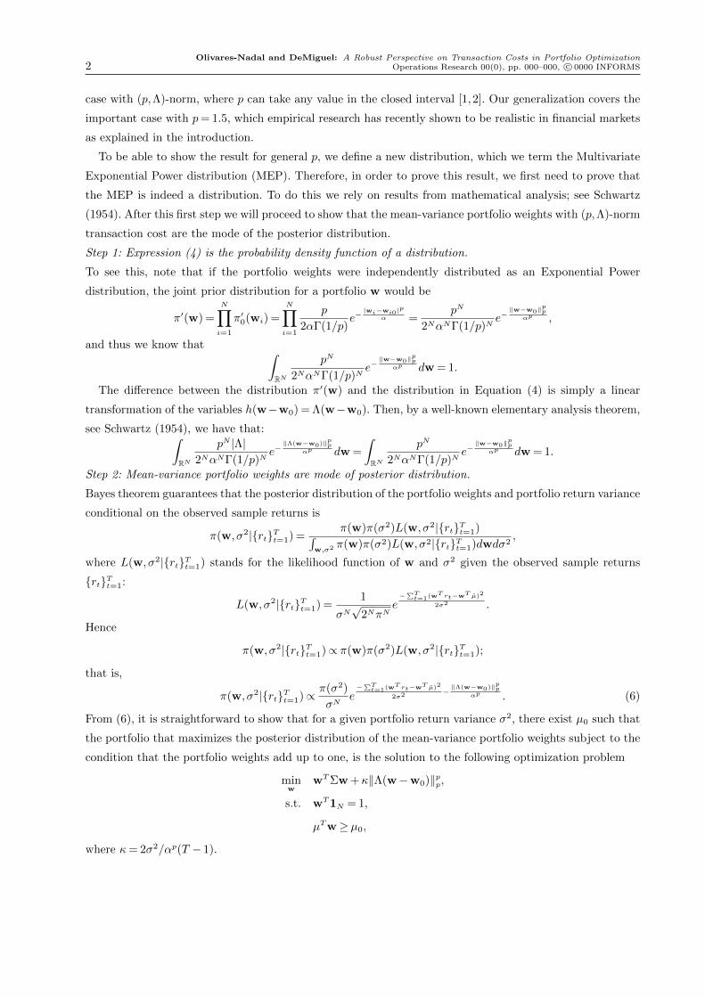
case with (p,Λ)-norm, where p can take any value in the closed interval [1,2]. Our generalization covers the
important case with p= 1.5, which empirical research has recently shown to be realistic in financial markets
as explained in the introduction.
To be able to show the result for general p, we define a new distribution, which we term the Multivariate
Exponential Power distribution (MEP). Therefore, in order to prove this result, we first need to prove that
the MEP is indeed a distribution. To do this we rely on results from mathematical analysis; see Schwartz
(1954). After this first step we will proceed to show that the mean-variance portfolio weights with (p,Λ)-norm
transaction cost are the mode of the posterior distribution.
Step 1: Expression (4) is the probability density function of a distribution.
To see this, note that if the portfolio weights were independently distributed as an Exponential Power
distribution, the joint prior distribution for a portfolio w would be
π′(w) =
N∏i=1
π′0(wi) =
N∏i=1
p
2αΓ(1/p)e−|wi−wi0|
p
α =pN
2NαNΓ(1/p)Ne−‖w−w0‖
pp
αp ,
and thus we know that ∫RN
pN
2NαNΓ(1/p)Ne−‖w−w0‖
pp
αp dw = 1.
The difference between the distribution π′(w) and the distribution in Equation (4) is simply a linear
transformation of the variables h(w−w0) = Λ(w−w0). Then, by a well-known elementary analysis theorem,
see Schwartz (1954), we have that:∫RN
pN |Λ|2NαNΓ(1/p)N
e−‖Λ(w−w0)‖pp
αp dw =
∫RN
pN
2NαNΓ(1/p)Ne−‖w−w0‖
pp
αp dw = 1.
Step 2: Mean-variance portfolio weights are mode of posterior distribution.
Bayes theorem guarantees that the posterior distribution of the portfolio weights and portfolio return variance
conditional on the observed sample returns is
π(w, σ2|{rt}Tt=1) =π(w)π(σ2)L(w, σ2|{rt}Tt=1)∫
w,σ2 π(w)π(σ2)L(w, σ2|{rt}Tt=1)dwdσ2,
where L(w, σ2|{rt}Tt=1) stands for the likelihood function of w and σ2 given the observed sample returns
{rt}Tt=1:
L(w, σ2|{rt}Tt=1) =1
σN√
2NπNe−
∑Tt=1(wT rt−wT µ)2
2σ2 .
Hence
π(w, σ2|{rt}Tt=1)∝ π(w)π(σ2)L(w, σ2|{rt}Tt=1);
that is,
π(w, σ2|{rt}Tt=1)∝ π(σ2)
σNe−
∑Tt=1(wT rt−wT µ)2
2σ2 −‖Λ(w−w0)‖pp
αp . (6)
From (6), it is straightforward to show that for a given portfolio return variance σ2, there exist µ0 such that
the portfolio that maximizes the posterior distribution of the mean-variance portfolio weights subject to the
condition that the portfolio weights add up to one, is the solution to the following optimization problem
minw
wTΣw+κ‖Λ(w−w0)‖pp,
s.t. wT1N = 1,
µTw≥ µ0,
where κ= 2σ2/αp(T − 1).

Olivares-Nadal and DeMiguel: A Robust Perspective on Transaction Costs in Portfolio OptimizationOperations Research 00(0), pp. 000–000, c© 0000 INFORMS 3
Appendix B: Tables and figures
Strategy 10Ind 48Ind 6FF 25FF CRSP
Panel A. Portfolios that ignore transaction costs, κ= 0
Minimum-variance, shortsale unconstrained 0.0106 0.0048 0.0136 0.0119 0.0139
Minimum-variance, shortsale constrained 0.0105 0.0101 0.0109 0.0103 0.0132
Mean-variance, shortsale unconstrained 0.0050 −0.2975 0.0179 −0.0014 −0.0012
Mean-variance, shortsale constrained 0.0101 0.0099 0.0123 0.0116 0.0108
Panel B. Portfolios with nominal transaction costs, 0.005‖∆w‖1
Minimum-variance, shortsale unconstrained 0.0119 0.0063 0.0132 0.0130 0.0153
Minimum-variance, shortsale constrained 0.0105 0.0111 0.0106 0.0103 0.0132
Mean-variance, shortsale unconstrained 0.0115 −0.1498 0.0150 −0.0132 0.0122
Mean-variance, shortsale constrained 0.0099 0.0106 0.0117 0.0122 0.0128
Panel C. Data-driven portfolios with calibrated proportional transaction costs, κcv‖∆w‖1
Minimum-variance, shortsale unconstrained 0.0120 0.0083 0.0138 0.0143 0.0152
Minimum-variance, shortsale constrained 0.0110 0.0113 0.0111 0.0111 0.0132
Mean-variance, shortsale unconstrained 0.0118 0.0046 0.0184 −0.1394 0.0146
Mean-variance, shortsale constrained 0.0107 0.0107 0.0114 0.0113 0.0125
Panel D. Data-driven portfolios with calibrated quadratic transaction costs, κcv‖Σ1/2∆w‖22
Minimum-variance, shortsale unconstrained 0.0118 0.0097 0.0144 0.0149 0.0154
Minimum-variance, shortsale constrained 0.0108 0.0109 0.0110 0.0108 0.0132
Mean-variance, shortsale unconstrained 0.0114 0.0259 0.0203 0.0286 0.0151
Mean-variance, shortsale constrained 0.0108 0.0110 0.0115 0.0116 0.0122
Table 3 Mean
This table reports the monthly out-of-sample means. The best mean for each dataset is highlighted in bold face.
Olivares-Nadal and DeMiguel: A Robust Perspective on Transaction Costs in Portfolio Optimization4 Operations Research 00(0), pp. 000–000, c© 0000 INFORMS
Strategy 10Ind 48Ind 6FF 25FF CRSP
Panel A. Portfolios that ignore transaction costs, κ= 0
Minimum-variance, shortsale unconstrained 0.0012 0.0017 0.0015 0.0015 0.0014
Minimum-variance, shortsale constrained 0.0013 0.0017 0.0019 0.0019 0.0011
Mean-variance, shortsale unconstrained 0.0053 11.1889 0.0069 0.0329 0.0168
Mean-variance, shortsale constrained 0.0023 0.0031 0.0024 0.0024 0.0024
Panel B. Portfolios with nominal transaction costs, 0.005‖∆w‖1
Minimum-variance, shortsale unconstrained 0.0016 0.0044 0.0019 0.0018 0.0015
Minimum-variance, shortsale constrained 0.0019 0.0018 0.0020 0.0020 0.0011
Mean-variance, shortsale unconstrained 0.0031 8.1876 0.0032 0.0795 0.0147
Mean-variance, shortsale constrained 0.0020 0.0027 0.0022 0.0022 0.0023
Panel C. Data-driven portfolios with calibrated proportional transaction costs, κcv‖∆w‖1
Minimum-variance, shortsale unconstrained 0.0013 0.0031 0.0018 0.0015 0.0015
Minimum-variance, shortsale constrained 0.0013 0.0015 0.0020 0.0019 0.0011
Mean-variance, shortsale unconstrained 0.0023 1.3320 0.0057 9.9690 0.0158
Mean-variance, shortsale constrained 0.0016 0.0023 0.0021 0.0021 0.0023
Panel D. Data-driven portfolios with calibrated quadratic transaction costs, κcv‖Σ1/2∆w‖22
Minimum-variance, shortsale unconstrained 0.0013 0.0017 0.0017 0.0016 0.0015
Minimum-variance, shortsale constrained 0.0013 0.0016 0.0020 0.0019 0.0011
Mean-variance, shortsale unconstrained 0.0020 6.0989 0.0070 0.3784 0.0161
Mean-variance, shortsale constrained 0.0015 0.0018 0.0021 0.0021 0.0023
Table 4 Variance
This table reports the monthly out-of-sample variances. The best variance for each dataset is highlighted inbold face
Olivares-Nadal and DeMiguel: A Robust Perspective on Transaction Costs in Portfolio OptimizationOperations Research 00(0), pp. 000–000, c© 0000 INFORMS 5
Strategy 10Ind 48Ind 6FF 25FF CRSP
Panel A. Portfolios that ignore transaction costs, κ= 0
Minimum-variance, shortsale unconstrained -0.0818 -0.0947 -0.0942 −0.1072 -0.0724
Minimum-variance, shortsale constrained −0.0909 −0.1146 −0.1155 −0.1142 −0.0840
Mean-variance, shortsale unconstrained −0.2113 −1.9423 −0.2037 −0.4666 −0.3284
Mean-variance, shortsale constrained −0.1288 −0.1810 −0.1410 −0.1441 −0.1237
Panel B. Portfolios with nominal transaction costs, 0.005‖∆w‖1
Minimum-variance, shortsale unconstrained −0.1000 −0.1676 −0.1031 −0.0951 −0.0808
Minimum-variance, shortsale constrained −0.1149 −0.1163 −0.1110 −0.1070 −0.0875
Mean-variance, shortsale unconstrained −0.1282 −0.9507 −0.1707 −1.2520 −0.2685
Mean-variance, shortsale constrained −0.1132 −0.1394 −0.1448 −0.1296 −0.1130
Panel C. Data-driven portfolios with calibrated proportional transaction costs, κcv‖∆w‖1
Minimum-variance, shortsale unconstrained −0.0976 −0.1314 −0.1145 -0.0938 −0.0808
Minimum-variance, shortsale constrained −0.0979 −0.1055 −0.1223 −0.1198 −0.0875
Mean-variance, shortsale unconstrained −0.1218 −2.7480 −0.1797 −0.5865 −0.2685
Mean-variance, shortsale constrained −0.1025 −0.1231 −0.1398 −0.1231 −0.1130
Panel D. Data-driven portfolios with calibrated quadratic transaction costs, κcv‖Σ1/2∆w‖22
Minimum-variance, shortsale unconstrained −0.0923 −0.1085 −0.1056 −0.1178 −0.0808
Minimum-variance, shortsale constrained −0.0963 −0.1071 −0.1238 −0.1248 −0.0875
Mean-variance, shortsale unconstrained −0.1091 −6.0924 −0.1800 −0.5984 −0.2685
Mean-variance, shortsale constrained −0.0996 −0.1136 −0.1420 −0.1260 −0.1134
Table 5 Value at risk
This table reports the monthly value at risk of the different portfolios for a confidence level of 1%. The bestVaR for each dataset is highlighted in bold face
Olivares-Nadal and DeMiguel: A Robust Perspective on Transaction Costs in Portfolio Optimization6 Operations Research 00(0), pp. 000–000, c© 0000 INFORMS
Strategy 10Ind 48Ind 6FF 25FF CRSP
Panel A. Portfolios that ignore transaction costs, κ= 0
Minimum-variance, shortsale unconstrained 3.7468 4.7145 4.7477 4.8522 3.4585
Minimum-variance, shortsale constrained 3.9438 8.7428 5.5980 5.8600 4.6902
Mean-variance, shortsale unconstrained 4.5280 260.6713 4.8322 4.1617 4.0493
Mean-variance, shortsale constrained 4.9890 5.1898 7.0514 6.2337 6.0823
Panel B. Portfolios with nominal transaction costs, 0.005‖∆w‖1
Minimum-variance, shortsale unconstrained 3.4872 5.4916 5.7466 5.5415 3.5537
Minimum-variance, shortsale constrained 3.9236 4.3366 5.2744 5.2073 4.6954
Mean-variance, shortsale unconstrained 3.3791 399.6804 8.1566 84.0081 4.3499
Mean-variance, shortsale constrained 3.9194 4.6733 6.3228 5.1141 6.9563
Panel C. Data-driven portfolios with calibrated proportional transaction costs, κcv‖∆w‖1
Minimum-variance, shortsale unconstrained 4.2407 6.2381 5.5368 5.0131 3.5706
Minimum-variance, shortsale constrained 4.0061 4.3379 5.5027 5.6622 4.6938
Mean-variance, shortsale unconstrained 3.5086 112.2207 21.5957 404.3720 4.5564
Mean-variance, shortsale constrained 4.1425 4.9611 5.9052 5.4618 6.8807
Panel D. Data-driven portfolios with calibrated quadratic transaction costs, κcv‖Σ1/2∆w‖22
Minimum-variance, shortsale unconstrained 3.9857 3.9538 5.5142 5.4337 3.5646
Minimum-variance, shortsale constrained 4.0325 5.4081 5.5643 5.4747 4.6987
Mean-variance, shortsale unconstrained 3.4827 106.6647 42.4249 246.5576 4.8191
Mean-variance, shortsale constrained 4.3336 4.8007 6.0423 5.4725 6.9713
Table 6 Kurtosis
This table reports the monthly kurtosis of the different portfolios. The best kurtosis for each dataset is highlighted
in bold face

Olivares-Nadal and DeMiguel: A Robust Perspective on Transaction Costs in Portfolio OptimizationOperations Research 00(0), pp. 000–000, c© 0000 INFORMS 7
Panel (a): Shortsale-unconstrained mean-variance
Panel (b): Shortsale-constrained mean-variance
Figure 1 Monthly out-of-sample returns of mean-variance portfolios for the 48Ind dataset.
This figure depicts the monthly out-of-sample returns of the shortsale-unconstrained (Panel (a)) and shortsale-
constrained (Panel (b)) mean-variance portfolios. The vertical axis represents absolute returns; that is, 0.2
corresponds to a 20% percentage return.