teaching probability: motivations from philosophy and...

Teaching Probability: Motivations from Philosophy and Practical Life

Magdalena Hykšová Faculty of Transportation Sciences, Czech Technical University, Czech Republic

Abstract

This paper describes several possibilities how to enliven usual probability classes. From the didactical point of view, one of interesting topics is the subjective interpretation of probability, which uses the principle of betting. The connection of betting rates with probabilities helps to demonstrate how probability theory and its abstract axioms relate to the real world. Students can also easily realize that unless they have better information than bookmakers, betting cannot bring them a long-run profit. Another topic discussed in this paper is geometric probability, a substantial tool for extracting quantitative information on spatial objects (human beings or animals and their organs, blood vessels, tissues, tumours, plants, rocks etc.) from probes of a lower dimension. Since we are surrounded and even formed by such structures, geometric probability plays an important role for exploring and understanding the world around us. Corresponding materials for classroom use are also presented. 1. Introduction

Probability theory seems to be in a rather paradoxical position. On one hand, we encounter it almost everywhere in our lives, we are surrounded by randomness, whether we speak about weather, natural disasters, traffic accidents or just delays, the organic world with tissue cells, vegetation and people themselves, the inorganic world with materials and their defects, the oil industry, geology, medicine, illnesses and the chances for healing or surviving, various polls, financial markets, hazards, spam detection, etc. The theory of probability therefore appears to be one of the most interesting and important disciplines, inseparably connected with our lives. On the other hand, in school mathematics, probability theory is often restricted to exercises concerning tossing coins, throwing dice or drawing balls from an urn – that is, to problems that do not seem a bit to relate to our everyday life. This is perhaps the main reason why so many students (and even many teachers) do not like probability and they class it as one of the least favourite parts of school mathematics. They consider it useless and, if it is possible, they try to avoid it. The aim of this paper is to contribute to the “rehabilitation” of probability theory, to draw the deserved attention to

this field and to point out its significance for school education: it is closely related to the life of each of us and thus it has an exceptional motivational potential for the study of mathematics and science in general, it helps teachers to demonstrate how science works, how it can help to solve many everyday problems, how important the philosophy of science is for science itself, what significance the history of science possesses for the present time, and at the more abstract level, that probability theory helps to clarify the relation between axiomatic theory and its interpretations and applications.

Naturally, there exist various books on probability and randomness in everyday life that clarify this close relation and provide interesting examples – let us mention at least the books by Gerd Gigerenzer [1], Michael and Ellen Kaplan [2] or Jeffrey S. Rosenthal [3]. This contribution is aimed at another two aspects. One of them concerns the so-called subjective interpretation of probability, the second one is connected with geometric probability. The reader interested in more details and study materials for classroom use is invited to visit the webpage [4]. 2. Probability interpretations

Recall that although most mathematicians agree with the axiomatic definition of probability in the sense of Kolmogorov’s foundations, philosophers and philosophically oriented mathematicians still search for the most convenient interpretation of probability introduced by this abstract definition. In other words, they search the best reply to a seemingly simple question of what probability actually is. Two groups of interpretations are usually distinguished (for more details, see [5]): the so-called epistemic interpretations that associate probability with the knowledge or belief of human beings, and objective interpretations that consider probabilities to be human-independent features of the objective material world.

Two principal objective interpretations are the frequency theory that defines probability of an outcome as the limiting frequency with which it appears in a long series of similar events, and the propensity theory that takes probability to be a propensity inherent in a set of repeatable conditions. In the domain of epistemic interpretations, the principal theories are called logical and subjective. The logical interpretation identifies probability with a degree of rational belief in a hypothesis or a

Literacy Information and Computer Education Journal (LICEJ), Volume 3, Issue 3, September 2012

Copyright © 2012, Infonomics Society 742

prediction; given the same evidence, all rational human beings would entertain the same probability. In this connection, let us only mention the extensive (in total 2397 pages) treatise Wissenschaftslehre [5] published by Bernard Bolzano (1781–1848) in the 1830’s, who developed probability theory as an extension of deductive logic and an integral part of the whole logical theory.

The subjective interpretation identifies probability with a degree of belief of a given individual in occurrence of some event or in the validity of some hypothesis. It was thoroughly investigated by the Czech priest and mathematician Václav Šimerka (1819–1887) at the beginning of the 1880’s (e.g. [6]), and independently of him by Bruno de Finetti (1906–1985) and Frank Plumpton Ramsey (1903–1933) (e.g. [7] and [8]) in the 1930’s. This approach deals with real concepts, with a subjective acceptance or rejection of hypothesis, and it thus corresponds to our frequent everyday considerations (for example, about the occurrence of a traffic jam, results of elections, sporting events, medical treatment, etc.) – whether we are conscious of it or not, we incessantly work with some personal probability assessments, although usually without their exact quantification.

3. Probability and betting rates

Nevertheless, one possibility how to evaluate subjective probability is also very well-known: it is sufficient to notice that it is exactly this problem which bookmakers face when setting betting rates for various sporting, political or social events. Although they try to gain maximum information, they still deal with chance and have to cope with it. Even the greatest enemy of probability theory knows that the typical published rates express how much the bettor gets for each staked Euro in the case of success, and the lower the rate, the higher the probability assigned by the bookmaker to the considered alternative. Thus, the most probable winner (at least according to a bookmaker) must always have the lowest rate.

Table 1. Illustration of betting rates

SPAIN DRAW HONDURASBet-at-home

1.11 8.0 15.0

Fortuna 1.12 6.7 13.0 Tipsport 1.13 8.1 15.05

For example, Table 1 illustrates the betting rates

of three different companies on a football match between Spain and Honduras and the highest probability is assigned for Spain to win.

Another question is, which betting company should be chosen? In our example, it is clear that whatever happens, Tipsport pays the most. More specifically, we can determine the so-called return of

our stake. This means, how many percent of the stake will be returned to us if we bet in such a way that whatever happens, we win a fixed amount of money. For example, consider Fortuna. To win 100 EUR in the case of Spain winning, we have to bet 100 divided by the corresponding rate on it, that is, 100/1.12, similarly for the other alternatives. It means, to win 100 EUR whatever happens, we have to stake 100/1.12 on Spain winning, 100/6.70 on a draw and 100/13.00 on Honduras winning. Altogether we have to pay

that is, almost 12 EUR more than we win. The

return is then the ratio of 100 to the just calculated value:

In other words, we get back slightly less than 90%

of our staked money. The same calculation can be repeated for the other betting companies. According to expectation, the highest return is provided by Tipsport: 93.04 %. Thus, students can observe that unless they have better information than the experienced and well-equipped staff of the betting company, or unless they have exceptionally good luck, betting cannot bring them a long-run profit. 3.1. Fair bets

The return R > 1 means that the bettor has a chance to guarantee himself a positive profit, whatever happens. On the other hand, R < 1 means a positive profit of the bookmaker. The only value, that seems to be fair for both sides, is R = 1. In this case, the inverse values of rates for mutually exclusive and exhaustive events would sum to 1 and they would be equal to probabilities assigned to particular events. As we can observe, the sum of these inverse values is always higher than 1 to generate bookmaker’s profit.

More general, let p denote the betting rate expressing directly the amount of money that must be staked to win 1 EUR if an event A occurs (it is therefore the inverse value of the usually published rate), S the win paid out to the bettor in the case of A (the corresponding stake is pS) and P(A) the bookmaker’s probability estimate. If A occurs, the bettor earns Z(A) = S − pS = (1−p) S, otherwise Z(¬A) = − pS; according to bookmaker’s opinion, bettor’s mean profit is Ž= P(A) (1−p)S + (1−P(A)) (−pS) = (P(A)−p) S. For any p > P(A), the mean profit of the bettor is negative and the bookmaker can expect a handsome income; such a bet can hardly be named “fair”. Similarly, any p < P(A) would lead to bookmaker’s sure loss. We can simply notice that the probabilities corresponding to the published rates are always more or less overestimated. Nevertheless,



to set the rates, bookmakers first need to estimate the true probabilities and only then they can adjust the values in their favour.

Now the natural question arises of how a fair bet can be achieved. One possibility was proposed by B. de Finetti [8] and it consists in admitting negative values of S: imagine that the bookmaker announces the rate p, then the bidder chooses S; if S < 0, the roles are exchanged and the bookmaker ends up in the position of the bettor (of course, it is not possible for betting companies, but, for example, for two betting people). Since he does not know the sign of S in advance, he is forced to be set the true value p = P(A). 3.2. Bets and probability axioms

From didactical point of view, betting is also interesting for the possibility to show students that the basic axioms of probability theory have not “come from above”, but they simply follow from the requirement of avoiding bookmaker’s sure loss, when S < 0 is admitted (such betting rates are called coherent):

1. For any event A, p = P(A) is the unique real

number satisfying 0 ≤ p ≤ 1. For p < 0, both Z(A) = (1−p) S and Z(¬A) = − pS

would be positive for any S > 0; for p > 1, the profit in both cases would be positive for any S < 0. If two different values p < p′ were announced, the bettor would have a chance to guarantee a sure profit by a convenient choice of his bets. For example, consider p = 0.4 and p′ = 0.6. The bettor can stake 40 EUR in the first rate and – 60 EUR in the second one. When event A occurs, he gets 100 – 40 = 60 EUR from the first stake and – 100 + 60 = – 40 EUR from the second one, in total he gains 20 EUR. When A does not occur, his profit is again – 40 + 60 = 20 EUR. In general, for any two different values p < p′ the bettor would win in any case by carrying out two bets on A: pS and p′ (− S) with S > 0; his profit would be.

2. If AE denotes a sure event with pE = P(AE) and

A denotes an impossible event with p = P(A ), then pE = 1, p = 0.

Since a sure event must occur, the bettor’s profit is always Z(AE) = (1−pE) S ; for p < 1, the bettor would achieve a positive profit by choosing any S > 0. For an impossible event, the profit Z(A ) = −p S would always be positive for any S < 0.

3a. Probability of a complementary event:

Denote the probabilities of the event A and

complementary event ¬ A by P(A)= p P(¬A)= q. We want to show that p+q = 1. Consider, for example, p=0.4 , q=0.5. To win 100 EUR in any case, the

bettor has to bet 40 EUR on event A and 50 EUR on ¬A. In total, he would pay 90 EUR and win 100 EUR, and the bookmaker would always lose 10 EUR; such probability estimation is therefore not coherent. The same holds for any two values of p, q with p+q < 1: to guarantee the win of 100 EUR, it is sufficient to pay (p+q) 100 < 100, which leads to a positive profit of the bettor. If p+q>1, then the bettor can propose a negative stake, for example −p 100 on event A and −q 100 on ¬ A. Now the bookmaker has to pay (p+q) 100 100 and wins only 100, which again violates the coherence requirement.

Thus the equality p+q=1 must hold. 3b. Additivity: r = p + q for any two mutually

exclusive events A, B with p = P(A), q = P(B), r = P(A B).

Consider three bets: pS on A, qS on B and (1−r)S on ¬ A ¬B. The bettor’s profit can be expressed as follows:

If p + q < r or p + q > r, then the profit would

always be positive for any S >0 or S < 0, respectively.

3c. Finite additivity: p1 + p2 + + pn = 1 for any

mutually exclusive and exhaustive events A1, A2, …, An with p1 = P(A1), p2 = P(A2), ..., pn = P(An).

Consider bets p1S, p2S, ..., pnS on A1, A2, …, An respectively. Now the bettor’s profit is always equal to Z(Ai) = (1 − p1 − p2 − − pn) S. If p1 + p2 + …+ pn <1 or p1 + p2 + + pn > 1, then the profit would again be positive for any S > 0 or S < 0, respectively.

Let us note that although B. de Finetti claimed that probability should be defined as the measure of the conviction of a particular individual, he admitted that its evaluation takes into account all available evidence including frequencies, symmetries etc. Nevertheless, in his opinion, it would be a mistake to treat these factors as the foundation of definition of probability. He points out that probability estimation is a complex process, where various subjective and objective elements play important roles:

− carefulness and experiences during gathering and evaluation of information,

− proper selection of relevant information, − economic considerations that can differ due to a

context, − skills of the evaluator, − an optimistic or pessimistic attitude, − extent of susceptivity by the newest data.

4. Natural frequencies

Before we definitively leave the domain of probability interpretations, let us remark that various



problems, where a conditional probability plays an important role, can be surprisingly simply solved by a method inspired by frequency theory. Instead of relative frequencies in the results of a repeated experiment, we can consider absolute frequencies in a convenient “population”. Let us illustrate this approach advocated by G. Gigerenzer [1] and I. Hacking [10] by the following example.

Before entering a new job, David has to undergo a routine medical check-up including an HIV test. The test producer claims that in the case of an ill person, the test detects the virus with the probability 99.90 %, and in the case of a healthy person, it gives the negative result with the probability 99.99 %. In the Czech Republic, approximately 1 person in 10 000 is infected by HIV (this is the so-called prevalence of the virus in the given population). After the evaluation of the test, the physician calls David and says he is positive and the test must therefore be repeated. Theresult of the second test will be known in one week. In the meanwhile, David has to wait, fearing the worst. As far as the danger of HIV infection is concerned, David considers himself to be an average Czech. What is the probability after the result of the first test that he is indeed infected by HIV?

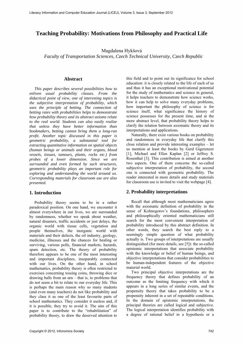
At the first sight, the situation seems hopeless. But when the percentages are replaced by a sort of frequencies, the solution is simple and clear: Consider 10 000 people from the given country. Among them, on average, one is infected and the remaining 9999 people are healthy. The infected person probably has a positive test (this probability is 0.9990); of the remaining 9999 healthy people, one (on average) also tests positive – see Figure 1.

Figure 1. False positivity example – tree form Of 10 000 people, two have a positive test: one of

them is ill, the other one is healthy. The probability that David is ill, provided his test was positive, is therefore 1/2. In other words, we have found the false positivity, which is – in our example – equal to 50 %. The solution is also clear from Table 2, which can be simply adapted to other conditions, e.g., to the prevalence of only 1 in 100 000 (if David has been very cautious) – in this case, the searched probability would be only 9.09 %.

Table 2. False positivity example – table form Prevalence: 1:10 000, P (infected| positive) = 50%

INFECTED HEALTHY TOTAL positive 1 1 2 negative 0 9998 9998 total 1 9999 10000

Prevalence: 1:100 000, P (infected | positive) =

9.09 % INFECTED HEALTHY TOTAL positive 1 10 2 negative 0 99989 99989 total 1 99999 100000

The preceding example also illustrates the

meaning of a conditional probability: the probability that David tests positive, provided he is healthy, is very low, only 0.01 % or 0.0001. Nevertheless, once he does, the probability of being infected is not as high as many people think. This probability is conditioned by the fact that the test is positive– and this simply means one of two possibilities: either David had the bad luck to be that one person in 10 000 with a false positive result, or he is indeed infected. Since the proportion of both “types” in the considered population is equal, the searched probability is 1/2. For the prevalence of only 1:100 000, the chance that a person with a positive test is healthy is even ten times higher than the chance that he is infected. 5. Geometric probability

Mathematically, geometric probability was introduced as the extension of the classical definition of probability to situations with an uncountable number of cases: counting favourable and all possible cases is just replaced by measuring relevant sets. For example, the probability that point X lying in set C lies also in subset B C is defined as the ratio

where m denotes a convenient measure of the

given set (for example, area or volume for sets in 2D or 3D, respectively). From this simple definition, useful applications immediately follow.

Recall that when we pass from the investigation of properties of finite populations to geometric properties (e.g., volume, area, length, shape) of geometrically describable objects (e.g., human beings and their organs and blood vessels, animals, plants, cells in a tissue, rivers, rocks etc.), replacing random population samples by probes of a lower dimension (sections or microscope images, linear or point probes), and instead of "classical" probability we base our inferences on geometric probability, we



pass from statistics to the domain of stereology. Since we are not only surrounded but even formed by such structures, stereology and hence also geometric probability are of great importance to our lives and represent a substantial tool for exploring and understanding the world around us. 5.1. Point counting and area estimation

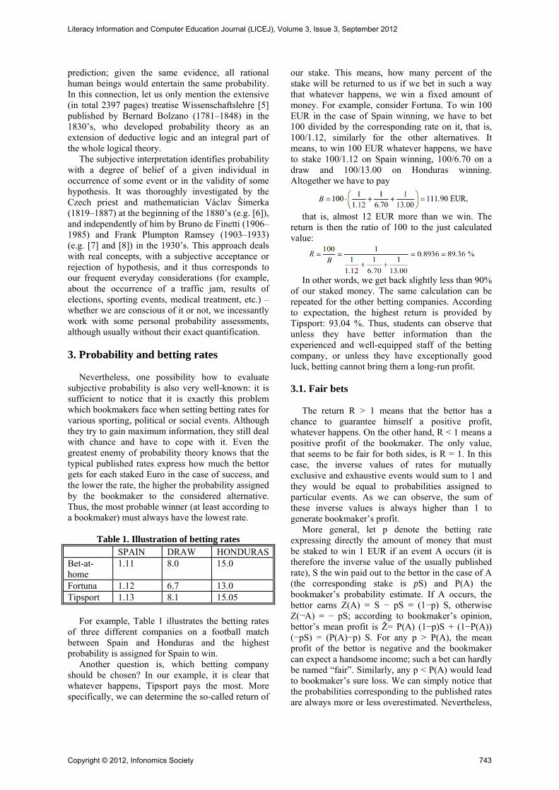
Consider sets B C in a plane. On one hand, the probability (1) is defined as the ratio of areas of B and C; on the other hand, it can be estimated by “throwing” random points on C and counting those hitting also B:

If the area A(C) is known, the equation (2) can

obviously be used for the estimation of the area A(B). Instead of “throwing” isolated random points, it is possible to place a transparent sheet with a point grid randomly and repeatedly on C (see Figure 2) and calculate the ratio of points hitting B and C. Finally, taking as C a rectangle with the area rs N formed by the grid, and using possibly the average number of hits in several repetitions, we obtain the direct estimation

Figure 2. Planar grid

This estimation technique is called the point

counting method. Note that it differs from the usually taught counting squares of a millimetre grid covering the investigated area. Here no attempt is made to estimate fractional parts around the perimeter; it is a statistical method, the accuracy of which is increased by increasing the number of repetitions.

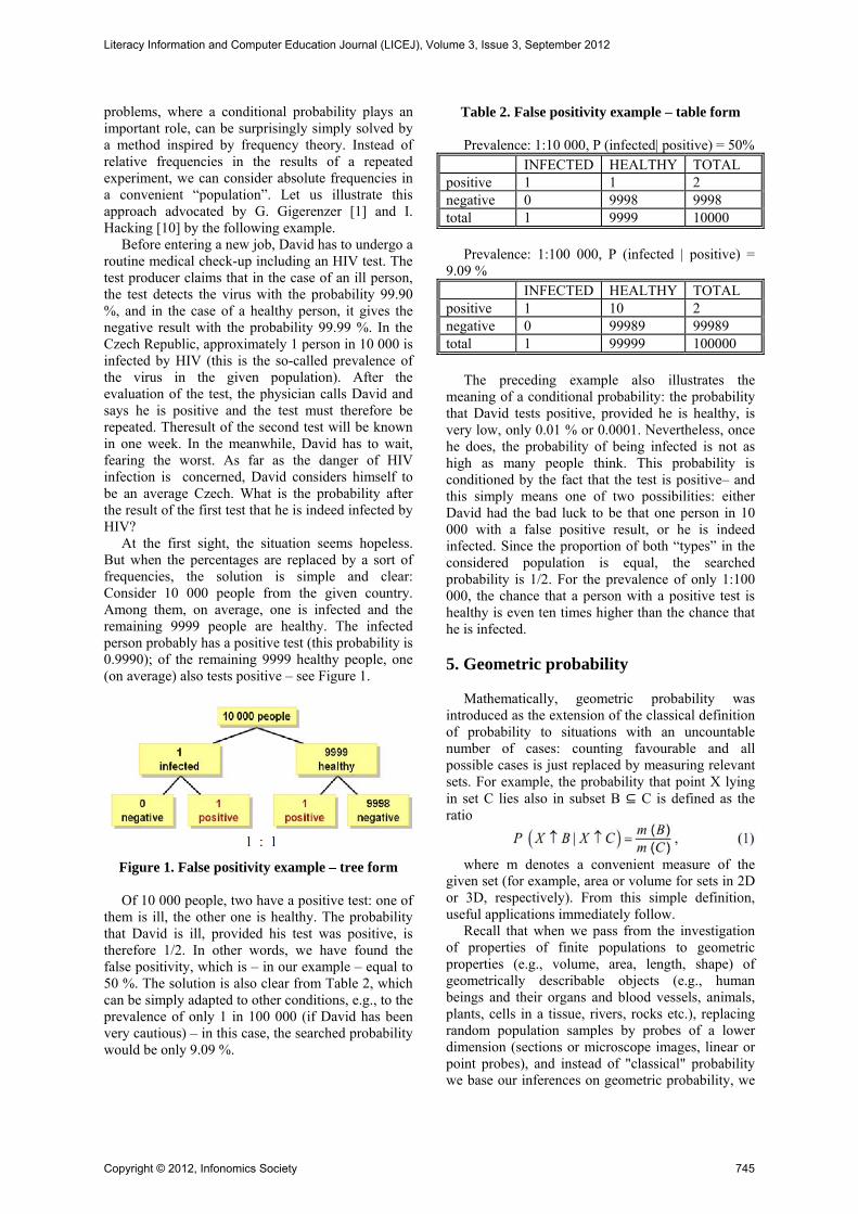
Figure 3. Aorta section

For classroom, the point counting method can be

used for the estimation of area of various lakes or lands on a map, as well as for the investigation of various biological objects or their images. Students can compare it with other methods that they can suggest and thus discover its advantage – particularly for complicated shapes (see Figure 3). Several worksheets for such experiments are available at the mentioned webpage [4] created by the author. 5.2. Volume estimation

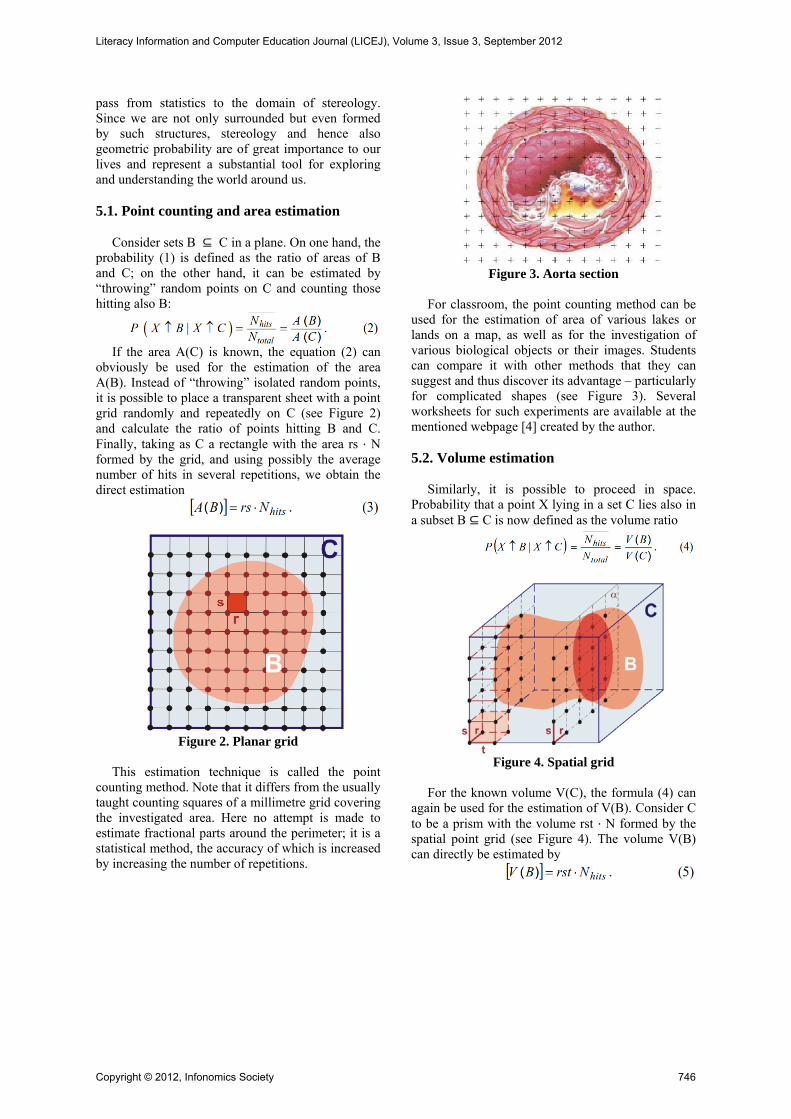
Similarly, it is possible to proceed in space. Probability that a point X lying in a set C lies also in a subset B C is now defined as the volume ratio

Figure 4. Spatial grid

For the known volume V(C), the formula (4) can

again be used for the estimation of V(B). Consider C to be a prism with the volume rst N formed by the spatial point grid (see Figure 4). The volume V(B) can directly be estimated by



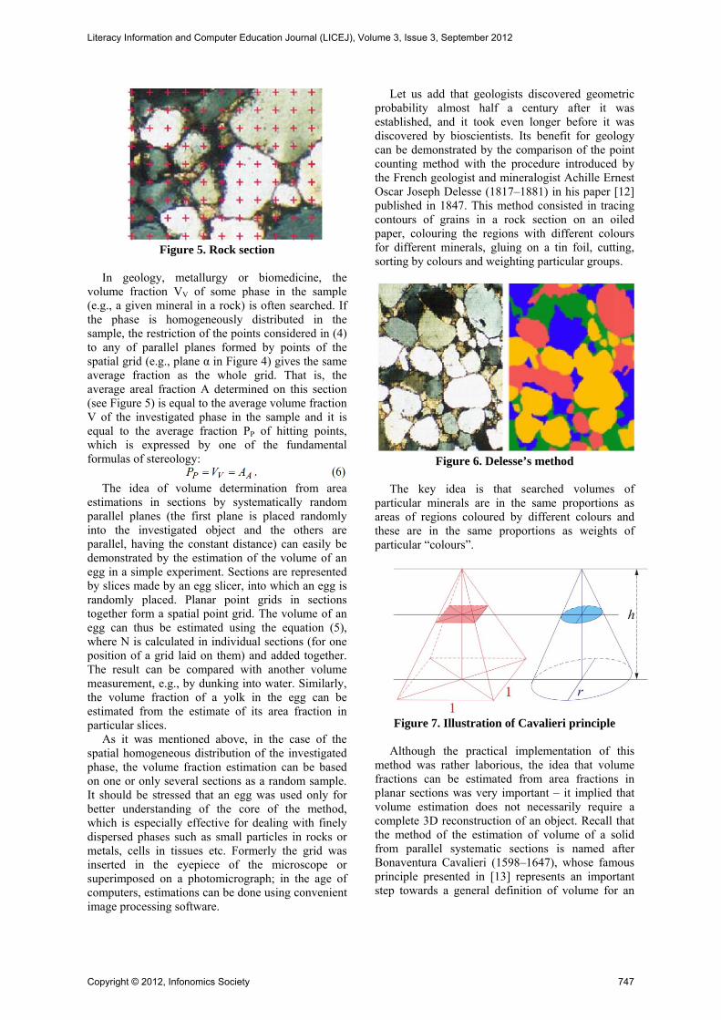
Figure 5. Rock section

In geology, metallurgy or biomedicine, the

volume fraction VV of some phase in the sample (e.g., a given mineral in a rock) is often searched. If the phase is homogeneously distributed in the sample, the restriction of the points considered in (4) to any of parallel planes formed by points of the spatial grid (e.g., plane α in Figure 4) gives the same average fraction as the whole grid. That is, the average areal fraction A determined on this section (see Figure 5) is equal to the average volume fraction V of the investigated phase in the sample and it is equal to the average fraction PP of hitting points, which is expressed by one of the fundamental formulas of stereology:

The idea of volume determination from area

estimations in sections by systematically random parallel planes (the first plane is placed randomly into the investigated object and the others are parallel, having the constant distance) can easily be demonstrated by the estimation of the volume of an egg in a simple experiment. Sections are represented by slices made by an egg slicer, into which an egg is randomly placed. Planar point grids in sections together form a spatial point grid. The volume of an egg can thus be estimated using the equation (5), where N is calculated in individual sections (for one position of a grid laid on them) and added together. The result can be compared with another volume measurement, e.g., by dunking into water. Similarly, the volume fraction of a yolk in the egg can be estimated from the estimate of its area fraction in particular slices.

As it was mentioned above, in the case of the spatial homogeneous distribution of the investigated phase, the volume fraction estimation can be based on one or only several sections as a random sample. It should be stressed that an egg was used only for better understanding of the core of the method, which is especially effective for dealing with finely dispersed phases such as small particles in rocks or metals, cells in tissues etc. Formerly the grid was inserted in the eyepiece of the microscope or superimposed on a photomicrograph; in the age of computers, estimations can be done using convenient image processing software.

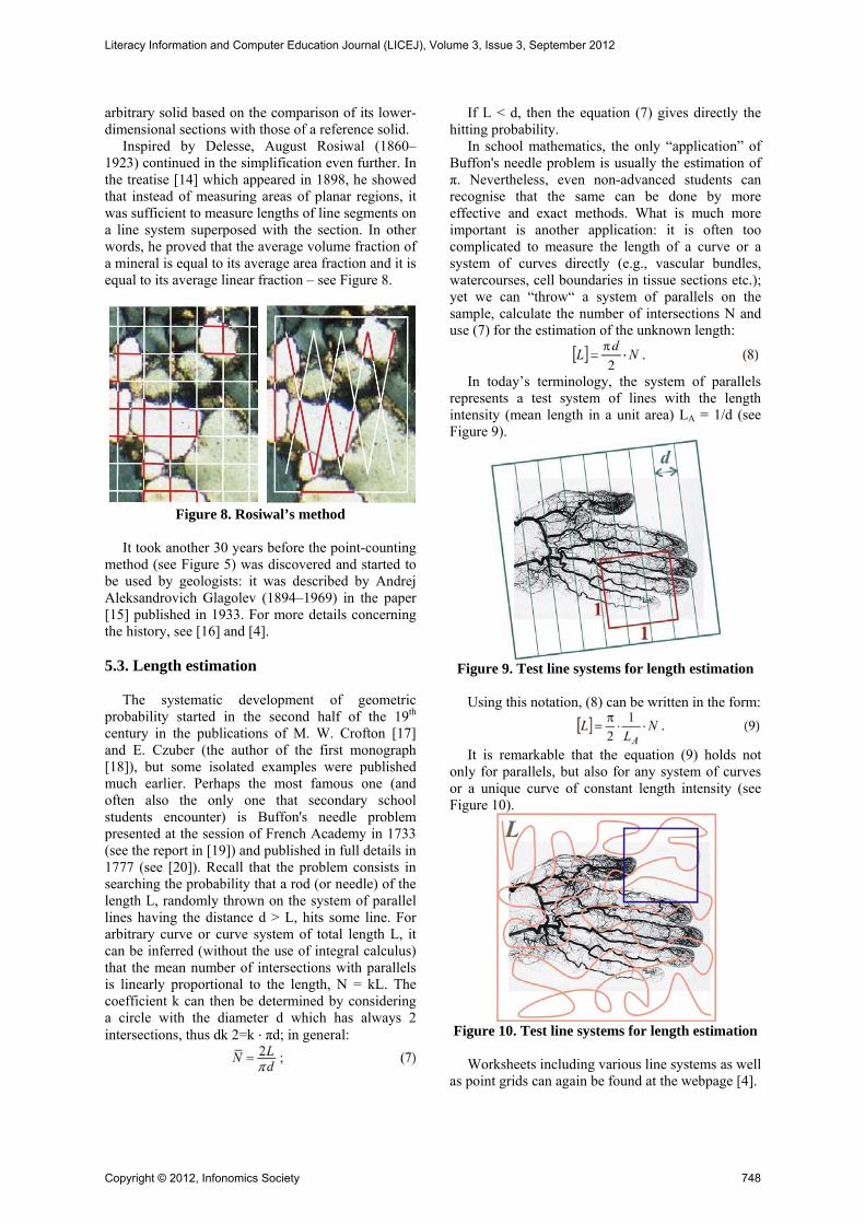
Let us add that geologists discovered geometric probability almost half a century after it was established, and it took even longer before it was discovered by bioscientists. Its benefit for geology can be demonstrated by the comparison of the point counting method with the procedure introduced by the French geologist and mineralogist Achille Ernest Oscar Joseph Delesse (1817–1881) in his paper [12] published in 1847. This method consisted in tracing contours of grains in a rock section on an oiled paper, colouring the regions with different colours for different minerals, gluing on a tin foil, cutting, sorting by colours and weighting particular groups.

Figure 6. Delesse’s method

The key idea is that searched volumes of

particular minerals are in the same proportions as areas of regions coloured by different colours and these are in the same proportions as weights of particular “colours”.

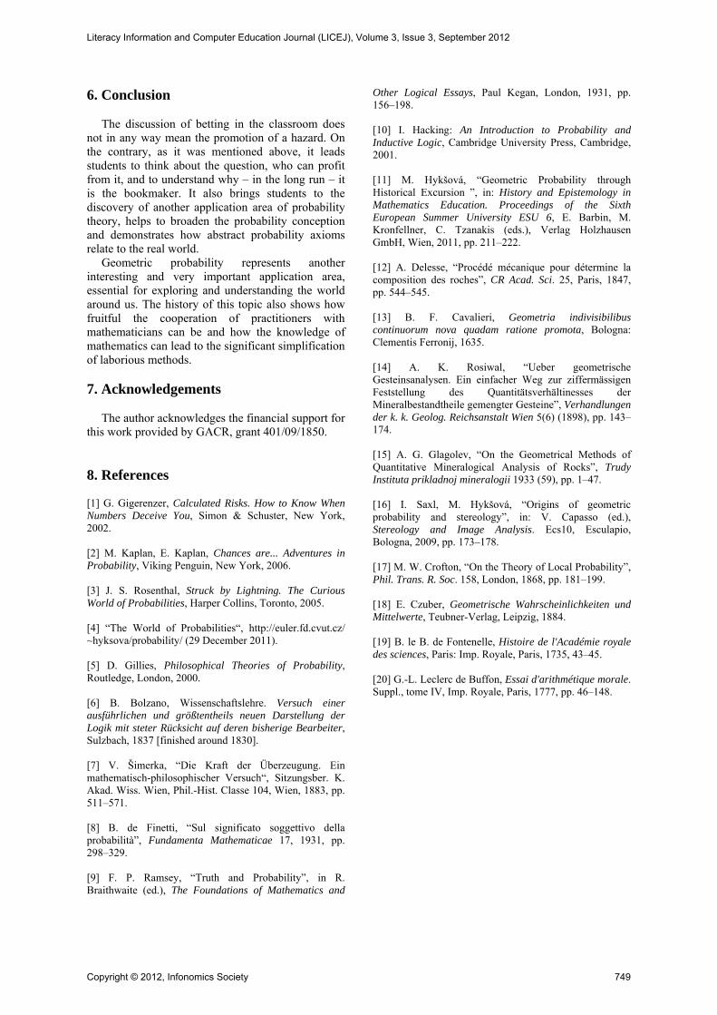
Figure 7. Illustration of Cavalieri principle

Although the practical implementation of this

method was rather laborious, the idea that volume fractions can be estimated from area fractions in planar sections was very important – it implied that volume estimation does not necessarily require a complete 3D reconstruction of an object. Recall that the method of the estimation of volume of a solid from parallel systematic sections is named after Bonaventura Cavalieri (1598–1647), whose famous principle presented in [13] represents an important step towards a general definition of volume for an



arbitrary solid based on the comparison of its lower-dimensional sections with those of a reference solid.

Inspired by Delesse, August Rosiwal (1860–1923) continued in the simplification even further. In the treatise [14] which appeared in 1898, he showed that instead of measuring areas of planar regions, it was sufficient to measure lengths of line segments on a line system superposed with the section. In other words, he proved that the average volume fraction of a mineral is equal to its average area fraction and it is equal to its average linear fraction – see Figure 8.

Figure 8. Rosiwal’s method

It took another 30 years before the point-counting

method (see Figure 5) was discovered and started to be used by geologists: it was described by Andrej Aleksandrovich Glagolev (1894–1969) in the paper [15] published in 1933. For more details concerning the history, see [16] and [4]. 5.3. Length estimation

The systematic development of geometric probability started in the second half of the 19th century in the publications of M. W. Crofton [17] and E. Czuber (the author of the first monograph [18]), but some isolated examples were published much earlier. Perhaps the most famous one (and often also the only one that secondary school students encounter) is Buffon's needle problem presented at the session of French Academy in 1733 (see the report in [19]) and published in full details in 1777 (see [20]). Recall that the problem consists in searching the probability that a rod (or needle) of the length L, randomly thrown on the system of parallel lines having the distance d > L, hits some line. For arbitrary curve or curve system of total length L, it can be inferred (without the use of integral calculus) that the mean number of intersections with parallels is linearly proportional to the length, N = kL. The coefficient k can then be determined by considering a circle with the diameter d which has always 2 intersections, thus dk 2=k πd; in general:

If L < d, then the equation (7) gives directly the hitting probability.

In school mathematics, the only “application” of Buffon's needle problem is usually the estimation of π. Nevertheless, even non-advanced students can recognise that the same can be done by more effective and exact methods. What is much more important is another application: it is often too complicated to measure the length of a curve or a system of curves directly (e.g., vascular bundles, watercourses, cell boundaries in tissue sections etc.); yet we can “throw“ a system of parallels on the sample, calculate the number of intersections N and use (7) for the estimation of the unknown length:

In today’s terminology, the system of parallels

represents a test system of lines with the length intensity (mean length in a unit area) LA = 1/d (see Figure 9).

Figure 9. Test line systems for length estimation

Using this notation, (8) can be written in the form:

It is remarkable that the equation (9) holds not

only for parallels, but also for any system of curves or a unique curve of constant length intensity (see Figure 10).

Figure 10. Test line systems for length estimation

Worksheets including various line systems as well

as point grids can again be found at the webpage [4].



6. Conclusion

The discussion of betting in the classroom does not in any way mean the promotion of a hazard. On the contrary, as it was mentioned above, it leads students to think about the question, who can profit from it, and to understand why – in the long run – it is the bookmaker. It also brings students to the discovery of another application area of probability theory, helps to broaden the probability conception and demonstrates how abstract probability axioms relate to the real world.

Geometric probability represents another interesting and very important application area, essential for exploring and understanding the world around us. The history of this topic also shows how fruitful the cooperation of practitioners with mathematicians can be and how the knowledge of mathematics can lead to the significant simplification of laborious methods.

7. Acknowledgements

The author acknowledges the financial support for this work provided by GACR, grant 401/09/1850.

8. References [1] G. Gigerenzer, Calculated Risks. How to Know When Numbers Deceive You, Simon & Schuster, New York, 2002. [2] M. Kaplan, E. Kaplan, Chances are... Adventures in Probability, Viking Penguin, New York, 2006. [3] J. S. Rosenthal, Struck by Lightning. The Curious World of Probabilities, Harper Collins, Toronto, 2005. [4] “The World of Probabilities“, http://euler.fd.cvut.cz/ ~hyksova/probability/ (29 December 2011). [5] D. Gillies, Philosophical Theories of Probability, Routledge, London, 2000. [6] B. Bolzano, Wissenschaftslehre. Versuch einer ausführlichen und größtentheils neuen Darstellung der Logik mit steter Rücksicht auf deren bisherige Bearbeiter, Sulzbach, 1837 [finished around 1830]. [7] V. Šimerka, “Die Kraft der Überzeugung. Ein mathematisch-philosophischer Versuch“, Sitzungsber. K. Akad. Wiss. Wien, Phil.-Hist. Classe 104, Wien, 1883, pp. 511–571. [8] B. de Finetti, “Sul significato soggettivo della probabilità”, Fundamenta Mathematicae 17, 1931, pp. 298–329. [9] F. P. Ramsey, “Truth and Probability”, in R. Braithwaite (ed.), The Foundations of Mathematics and

Other Logical Essays, Paul Kegan, London, 1931, pp. 156–198. [10] I. Hacking: An Introduction to Probability and Inductive Logic, Cambridge University Press, Cambridge, 2001. [11] M. Hykšová, “Geometric Probability through Historical Excursion ”, in: History and Epistemology in Mathematics Education. Proceedings of the Sixth European Summer University ESU 6, E. Barbin, M. Kronfellner, C. Tzanakis (eds.), Verlag Holzhausen GmbH, Wien, 2011, pp. 211–222. [12] A. Delesse, “Procédé mécanique pour détermine la composition des roches”, CR Acad. Sci. 25, Paris, 1847, pp. 544–545. [13] B. F. Cavalieri, Geometria indivisibilibus continuorum nova quadam ratione promota, Bologna: Clementis Ferronij, 1635. [14] A. K. Rosiwal, “Ueber geometrische Gesteinsanalysen. Ein einfacher Weg zur ziffermässigen Feststellung des Quantitätsverhältinesses der Mineralbestandtheile gemengter Gesteine”, Verhandlungen der k. k. Geolog. Reichsanstalt Wien 5(6) (1898), pp. 143–174. [15] A. G. Glagolev, “On the Geometrical Methods of Quantitative Mineralogical Analysis of Rocks”, Trudy Instituta prikladnoj mineralogii 1933 (59), pp. 1–47. [16] I. Saxl, M. Hykšová, “Origins of geometric probability and stereology”, in: V. Capasso (ed.), Stereology and Image Analysis. Ecs10, Esculapio, Bologna, 2009, pp. 173–178. [17] M. W. Crofton, “On the Theory of Local Probability”, Phil. Trans. R. Soc. 158, London, 1868, pp. 181–199. [18] E. Czuber, Geometrische Wahrscheinlichkeiten und Mittelwerte, Teubner-Verlag, Leipzig, 1884. [19] B. le B. de Fontenelle, Histoire de l'Académie royale des sciences, Paris: Imp. Royale, Paris, 1735, 43–45. [20] G.-L. Leclerc de Buffon, Essai d'arithmétique morale. Suppl., tome IV, Imp. Royale, Paris, 1777, pp. 46–148.



teaching probability: motivations from philosophy and...

Documents