taxpayers’choices under studi di settore ... ’choices under studi di settore 163 individual...

Giornale degli Economisti e Annali di EconomiaVolume 67 - N. 2 (Luglio 2008) pp. 161-184

TAXPAYERS’CHOICES UNDER STUDI DI SETTORE: WHAT DO WE KNOW AND HOW WE CAN INTERPRET IT?

ALESSANDRO SANTORO1

Received: September 2007; accepted: March 2008

Studi di settore (Sds) can be seen as a procedure that is midway between mechanisms

of audit selection and methods of normal taxation. Its impact depends both on the effi-

ciency of the audit selection criteria as well as on the strength of the political compro-

mise that is built-in. This paper has three purposes. The first is to construct a simple

model of the firm’s choice under Sds. The second is to use the model to discuss the styl-

ized facts emerging from the implementation of Sds in the period 1998-2004. The third

is to provide some policy indications to evaluate recent amendments to Sds.

JEL Classification: H25, H26, K42. Keywords: tax, evasion, audit.

1. INTRODUCTION

“Studi di settore” (Sds, or ‘business sector analyses’) were introduced inItaly in 1998; however, their nature and interpretation is rather controver-sial (Arachi-Santoro, 2007). Sds are basically audit selection mechanisms: asmall or medium sized firm (which is the taxpayer, TP, in this paper) can beaudited if it reports a level of turnover (sales proceeds) that is lower thanthe presumed level. The latter depends primarily on the value of inputs asreported by the firm.2 However, the presumed level also depends on the av-

1 Alessandro Santoro, DSGE, Università degli studi di Milano-Bicocca e Econpubbli-ca (Università Bocconi), Piazza dell'Ateneo Nuovo 1, 20126 Milano, ++390264484081 (tele-phone) ++390264484110 (fax), [email protected]. I wish to thank Massimo Bor-dignon, Giulio Zanella, Stefano Pisani, Lucia Visconti Parisio, Bruno Bosco, GiampaoloArachi, an anonymous referee and all participants at the conference New Issues in Eco-nomic Policy, for their very helpful suggestions. The usual disclaimers apply.

2 Thus, Sds are based on an endogenous threshold, while the optimal audit scheme(with commitment), suggested in the literature, requires an entirely exogenous threshold(Andreoni et al., 1998; Sanchez and Sobel, 1993). It would be interesting to explore theo-retically whether the differences between Sds and the optimal audit procedures suggestedin the literature are actually justified by the specific context in which Sds are designed, suchthat Sds may in fact be conditionally optimal. In this paper, however, we propose that sucha design, rather than being inspired by the search for an optimal auditing scheme, can beunderstood by considering it not just as an audit selection mechanism.

02 - santoro 28-07-2008 9:55 Pagina 161

162 ALESSANDRO SANTORO

erage productivity of the firms within the same business sector. Thus, Sdscan also be regarded as indirect methods of normal or presumptive taxationsimilar to those applied in many other countries, although no presumptivetax is formally levied. Finally, there is another interpretation of Sds that isgrounded in political economy. Some organizations representing small andmedium sized firms, which we will call ‘TP’s representatives’, are deeply in-volved in the process of calculating the presumed level of turnover and inthe implementation of Sds, as we describe in Section 2. Thus, many arguethat Sds should be seen as the outcome of a political compromise betweensmall and medium firms and the Tax Agency.

To sum up, Sds can be seen as being midway between application of au-dit selection mechanisms and methods of presumptive (normal) taxationwhose impact depends on the efficiency of the audit selection criteria as wellas on the strength of the built-in political compromise. In this paper we mod-el the TP’s choice based mainly on the first line of interpretation (Sds as au-dit selection mechanisms) but, in order to try to explain the stylized facts,we make reference in the last part of the paper to a more ‘political’ argument.

This paper has three main objectives. First, to construct a simple mod-el of firm's choice under Sds; second to use this model to discuss the styl-ized facts emerging from the implementation of Sds in the period 1998-2004and third, to formulate some policy suggestions.

The paper is structured as follows. In Section 2 we describe the mainfeatures of Sds and highlight the stylized facts emerging from their imple-mentation in the period 1998-2004. In Section 3 we construct a simple mod-el of the TP’ choice under Sds on the basis of Scotchmer (1987) and Cowell(2003). In Section 4 we provide some theoretical findings, which are dis-cussed in Section 5. Section 6 reports the results of a numerical simulationbased on actual data in order to try to capture the main features of the 1998-2004 period. Section 7 provides some concluding remarks on the policy im-plications of the paper.

2. DESCRIPTION OF AND SOME STYLIZED FACTS RELATING TO SDS

Sds are audit selection mechanisms based on a sophisticated statisticalprocedure that signals firms that report an ”implausibly low” level ofturnover. Sds were introduced in 1998 after lengthy debate and, since then,have progressively grown in importance; in fiscal year 2004 70% of Italianfirms, i.e. around 4 million taxpayers, were eligible to be audited on thebasis of Sds.

We describe below a typical Sds for a given business sector. Initially, da-ta are collected from all firms (corporated and unincorporated companies,

02 - santoro 28-07-2008 9:55 Pagina 162

TAXPAYERS’CHOICES UNDER STUDI DI SETTORE 163

individual entrepreneurs, self-employed people) reporting an annualturnover not greater than 5.164.569 euros. Data include structural variables-such as surface area of offices and warehouses, number of employees, typeof customers and so on- and accounting variables, mainly costs. Principalcomponents analysis (PCA) is applied in order to select from all those col-lected, the structural variables that are statistically the most significant.These variables are then used to construct the clusters, the key element ofthe statistical procedure. Specifically, all the firms belonging to a cluster arehomogeneous with respect to the structural variables selected by PCA.

Having defined the concept of a cluster we now briefly illustrate how Sdswork. Sds can generate two types of audits. A firm is liable for a type I au-dit if and only if it reports a turnover value that is lower than the presumed(normal) level. The presumed level of turnover is calculated as the productof a vector of values reported by the firm, and their corresponding parame-ters. The values refer to a set of independent variables, which are statisticallyassociated with turnover; in this paper we define these variables as the rel-evant (independent) variables. Essentially, the relevant independent variablesare physical and economic inputs. For example, for the real estate sector, themain relevant independent variables are square metreage and number ofrented houses and buildings, the value of capital goods, the cost of services,and the cost of labour. The parameters, resulting from an econometric in-vestigation, reflect the average relationship between the relevant independ-ent variables and turnover, for a subset of firms belonging to the same clus-ter and satisfying a given ‘consistency criterion’. This criterion, in turn, isbased on the cumulative distribution of indicators such as value added perworker, inventory turnover and the ratio of sales to the book value of capi-tal assets.

In this paper, the presumed level of turnover is denoted by βXi where Xi

is the vector of the relevant independent variables and β is the associated vec-tor of parameters. This value has to be compared with the reported turnover,which we denote with Ri. If the firm reports a turnover value that is lowerthan the presumed value and it is actually audited, the penalty that can beapplied is largely discretionary since it is the outcome of a sort of bargain-ing process between the Tax Agency and the TP (it belongs to the procedureknown as accertamento con adesione). This is a notable change with respectto what is commonly assumed in theoretical models, i.e. that penalties areset by the law and known by every taxpayer. Setting aside the possibility ofimperfect knowledge of the legal rules, the important point here is that thepenalty in type I audits depends on a number of variables such as the atti-tude of the responsible tax officer, the ability of the TP to argue that Ri < βXi,the local office’s revenue target and so on.

02 - santoro 28-07-2008 9:55 Pagina 163


In type II audits, the firm may be audited on the difference between re-ported values of relevant independent variables and their true value. Type IIaudits are the logical counterpart of type I audits. Clearly, if β > 0, firms canescape type I audits by simply underreporting X. Therefore, reports of Xshould be audited. However, for some years, this simple reasoning has notprevailed. Tax authorities, taxpayers and their representatives have focusedalmost exclusively on type I audits. Until 2004 type II audit activity was vir-tually zero and this helps to explain TP’s behaviour in the period 1998-2004demonstrated in this paper.

The two types of audits are obviously intertwined, but intrinsically dif-ferent. Type I audits are about the difference between TP’s presumed and re-ported turnover. There can be a number of reasons for this difference, suchas a temporary halt in production, a change in the structure of the market,indisposition of the entrepreneur (recall that we are dealing with small andmedium sized enterprises – SMEs), and so on. Type II audits are simpler,since they are based exclusively on the difference between the actual and thereported value of , although if such the audit has a positive outcome the TP’sentire tax liability must be recalculated.

What is the role of the TP’s representatives in this process? Their role isa prominent one. These representatives are gathered together in an expertcommittee – the Comitato degli Esperti – which is required to pass opinionon the ability of every Sds to actually represent the economic reality of thebusiness sector to which it is applied. Although this opinion does not repre-sent a formal commitment, and a single Sds may be enacted even if the TP’srepresentatives are not in agreement with it, it is politically very importantand, so far, all Sds have been ‘approved’ by this committee. Moreover, it iswell known that TP’s representatives are asked to state their views about thedifferent steps of the procedure, such as the choice of data being demand-ed, the selection of clusters and relevant (independent) variables and so on.In sum, TP’s representatives are closely involved in the Sds calculation andin the implementation process.

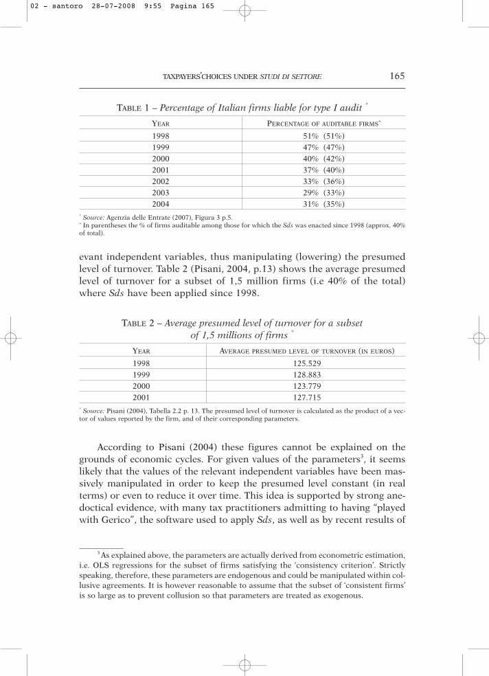
We next present some stylized facts (hereafter referred to as SFs). Table1, which is derived from Agenzia delle Entrate (2007), shows that the per-centage of firms liable for a type I audit has declined in the period 1998-2004.

This means that a growing percentage of firms have reported aturnover not lower than the presumed one (SF #1). At first sight this trendwould seem to confirm the effectiveness of Sds in inducing compliancewith the tax system since it should mean that, over time, firms have in-creased their average reported levels of turnover. However, there are someadditional facts that need to be considered. These include evidence sup-porting the idea that firms are inaccurately reporting the values of the rel-

02 - santoro 28-07-2008 9:55 Pagina 164


evant independent variables, thus manipulating (lowering) the presumedlevel of turnover. Table 2 (Pisani, 2004, p.13) shows the average presumedlevel of turnover for a subset of 1,5 million firms (i.e 40% of the total)where Sds have been applied since 1998.

3 As explained above, the parameters are actually derived from econometric estimation,i.e. OLS regressions for the subset of firms satisfying the ‘consistency criterion’. Strictlyspeaking, therefore, these parameters are endogenous and could be manipulated within col-lusive agreements. It is however reasonable to assume that the subset of ‘consistent firms’is so large as to prevent collusion so that parameters are treated as exogenous.

TABLE 1 – Percentage of Italian firms liable for type I audit *

YEAR PERCENTAGE OF AUDITABLE FIRMSˆ

1998 51% (51%)

1999 47% (47%)

2000 40% (42%)

2001 37% (40%)

2002 33% (36%)

2003 29% (33%)

2004 31% (35%)* Source: Agenzia delle Entrate (2007), Figura 3 p.5.ˆ In parentheses the % of firms auditable among those for which the Sds was enacted since 1998 (approx. 40%of total).

TABLE 2 – Average presumed level of turnover for a subset of 1,5 millions of firms *

YEAR AVERAGE PRESUMED LEVEL OF TURNOVER (IN EUROS)

1998 125.529

1999 128.883

2000 123.779

2001 127.715* Source: Pisani (2004), Tabella 2.2 p. 13. The presumed level of turnover is calculated as the product of a vec-tor of values reported by the firm, and of their corresponding parameters.

According to Pisani (2004) these figures cannot be explained on thegrounds of economic cycles. For given values of the parameters3, it seemslikely that the values of the relevant independent variables have been mas-sively manipulated in order to keep the presumed level constant (in realterms) or even to reduce it over time. This idea is supported by strong ane-doctical evidence, with many tax practitioners admitting to having “playedwith Gerico”, the software used to apply Sds, as well as by recent results of

02 - santoro 28-07-2008 9:55 Pagina 165


a statistical analysis (whose main results are available on the Italian gov-ernment’s website). The manipulation of the relevant independent variablescan thus be looked on as the second stylized fact (SF #2).

The third SF is that the percentage of firms that have actually been sub-jected to type II audits was negligible in the period 1998-2004. In particular,no specific monitoring activity on the values of X ’s reported by taxpayers waseither announced or planned by the Tax Agency up to 2004. As a conse-quence, we can assume that the expected penalty was perceived as being verylow for the entire period 1998-2004 (SF #3).

3. THE MODEL

The model used is based on a combination of the models proposed byScotchmer (1987) and Cowell (2003), adapted to take account of the legaland institutional framework of the design and implementation of Sds.

The TP is a risk-neutral firm which aims at minimizing the amount of itsexpected tax liability (as in Scotchmer, 1987) gross of the concealment costG generated by tax evasion. The idea (Cowell, 2003) is that tax-evasion is acostly activity since it entails organizational costs (manipulation of currentaccounts, implementation of a collusion agreement between employers andemployees) and possibly also psychological costs. In Cowell (2003) the cru-cial feature G of is its convexity with respect to the amount of tax evasion.The assumption of increasing marginal concealment cost enables some in-teresting results even when risk-aversion is not explicitly accounted for. Al-so, we note that the sign of the second derivative of G plays an importantrole in our model.

We follow the literature on tax evasion by firms (see Myles, 1997 for asummary) by assuming proportional taxes. This implies that our model mayapply to taxes such as Ires (the Italian tax on corporations) and Irap (the Ital-ian tax on value added) but generally not to Irpef (the Italian tax on indi-viduals, including unincorporated businesses and self-employed people).However, the analysis does apply to Irpef if the change in the tax base holdsthe TP within the same bracket.

We depart from the literature on tax evasion to specify the audit function.The usual assumption in the literature on optimal audits (Andreoni et al.,1998, Sanchez and Sobel, 1993) is that audits are aimed at detecting the truelevel of profits, but this is not the case in the Sds legal structure.

As explained in Section 2, there are two possible types of audits basedon Sds.

A type I audit may be applied when the turnover reported by the TP islower than the presumed (normal) level of turnover. This latter depends in

02 - santoro 28-07-2008 9:55 Pagina 166


part on a set of relevant variables as reported by the TP and in part on thefeatures of the economic sector to which the TP belongs. These features arecaptured by a set of parameters. The application of these parameters to thecorresponding set of reported independent variables generates the presumedlevel of turnover for the TP. To simplify the notations, and without loss ofgenerality, we consider only one reported variable and the value of its cor-responding parameter. The type I audit function can then be expressed byq(Ri < βXi) where Ri is the reported turnover, β > 04 is the parameter and Xi

is the reported level of the relevant variable. We now briefly describe themain properties of q(.).

There are two main legal and institutional constraints concerning typeI audits. First, when the turnover is (at least) equal to the presumed level,the TP is not liable for a type I audit. Second, the probability of being au-dited is “small” when the difference between Ri and βXi is also not large.5 Tomodel these constraints in a proper manner, we assume that, from the view-point of the TP, the audit function takes the following specification

(1)

In other words, we assume a linear decreasing audit function satisfyingq(1) = 0 where δ is inversely related to the steepness of the type I audit func-tion: a smaller δ means a steeper type I audit function, and viceversa.

Type II audits may be based on the difference between the true and thereported levels of the relevant variables.6 Since there are no explicit legal con-straints, we just assume that there is a nonnegative constant probability p of

q R XR

XR X

q R X

i ii

i

i i

( ˆ ˆ )ˆ

ˆˆ ˆ

ˆ ˆ

/ = − , ≤

= , >

βδ δ β

β

β

1 1

0

4 The assumption β > 0 is plausible since the overwhelming majority of relevant vari-ables are positively correlated with turnover.

5 To be more precise, the law states that a type I audit can be conducted only if the dif-ference between Ri and βXi is serious (“grave”). In practice this criterion has lead to dif-ferentiate between taxpayers reporting Ri < βXi – CV and taxpayers reportingβXi > Ri > βXi – CV, where CV > 0 is a confidence value associated to the econometric esti-mation of β (see Section 2). The probability to be audited is higher in the the former case.Strictly speaking, this assumption would lead to a bracket-structure of q(.). However, we as-sume here that q(.) is continuous since the Tax Agency is believed to audit more frequent-ly TPs reporting a larger value of βXi – Ri. This is plausible given that the Tax Agency hasan incentive to focus on more productive audits to meet its revenue targets.

6 We take the relative rather than the absolute difference since we have assumed β > 0so that reporting Xi > Xi is never profitable (it would increase both the expected penalty ofa type II audit and the difference βXi – Ri).

02 - santoro 28-07-2008 9:55 Pagina 167


a type II audit and that the corresponding penalty applies to the weighteddifference between the true and the reported level of the relevant variable,i.e to β(Xi – Xi).

Finally, we embody the concealment cost in the analysis asG = G(Xi – Xi) where G' > 0 since the TP has to modify its current accounts(if Xi is an accounting variable) or the structure of its firm (if Xi is a struc-tural variable which we assume can be measured) in the event of a type IIaudit. We also adopt Cowell’s (2003) assumption of convexity, thus G" > 0.

To sum up, the TP minimizes his total expected payment (EP) defined as

(2)

with respect to Ri and Xi, where Ci denotes the reported costs that are dif-ferent from the variable Xi,

7 f ’s are unitary penalties for the two types of au-dits and τ is the proportional tax rate.

Some comments concerning (2) are in order. First, one might think thatthe assumption of convexity of G(.), although common in the literature, isnot appropriate here and, more specifically, that there may be increasing re-turns to scale in tax evasion. Second, and relatedly, it could be argued thatunderreporting turnover is also costly, so that concealment costs would de-pend also on the difference between Ri and βXi. Let us tackle these two is-sues together.

In a conventional audit procedure, based on the difference between re-ported turnover Ri and true turnover Ri economies of scale would almost cer-tainly emerge. To conceal turnover it is necessary to instruct workers ap-propriately and to keep ‘black’ accounting. Once initiated, these activities arelikely to have low or zero marginal cost. However, type I audits are not fo-cused on the true turnover Ri, but rather on the difference between Ri andβXi. In other words, choosing a given level of turnover to report is not asso-ciated with the concealment of actual turnover, and, within some limits,there is no difference in the concealment cost if a high or a low level of Ri.is chosen. This explains why does not depend on the difference between Ri

and βXi. We now need to explain why we retain the assumption of convexity of

G(.). This is associated with the nature of X’s as either accounting or struc-tural variable. The manipulation of an accounting variable, in order to becredible, should be accompanied by manipulation of other variables. For ex-

EP R C q f X R p f X X G X Xi i i i i i i i= −( ) + . + −( ) + + − + −

τ τ β τβˆ ˆ ( )( ) ˆ ˆ ( ) ˆ ( ˆ )1 11 2

7 If the variable Xi is a cost, then this cost is not included in the vector Ci. Note alsothat Ci, strictly speaking, is a choice variable. However it is clear from the expression of EPthat the TP will select the highest possible value of Ci.

02 - santoro 28-07-2008 9:55 Pagina 168


ample, to credibly manipulate (underreport) the value of capital goods, thevalue of depreciation must be decreased. However, the accounting structureis, to some extent, rigid, so that the cost of manipulation, although perhapsnot continuously, is increasing in the amount of manipulation. On the oth-er hand, some structural variables are physical inputs whose concealmentmay also be increasingly costly (although again not necessarily in a contin-uous manner). Take, for example, a restaurant. Here, an important structuralvariable would be the number of tables used. It is plausible to assume thatconcealing the first n tables is less costly than concealing the n + 1th, when,for example, there is no available space to hide the n + 1th table in the eventof an audit.

Finally, the penalty in the case of type II audit is calculated on the basisof τβ rather than on the difference (Xi – Xi) to reflect the fact that when typeII audit is conducted tax officers are required to recalculate the whole tax li-ability.

4. THE RESULTS

Differentiating (2) with respect to Ri and Xi yields

(3)

(4)

where the partial derivatives of q with respect to Ri and Xi are denoted re-spectively by and .

Using (1) as the specification for q(.) we obtain (see Appendix)

(5)

which is the necessary and sufficient condition for the tax-minimizing Ri,given Xi. In accordance with the intuition, for a given f1, the steeper the q(.),i.e. the smaller the δ, and the closer Ri would be to βXi. This means that, ifXiwere not manipulable, (5) would provide the solution to the TP’s problem.

However, Xi is manipulable and, using (1), its optimal value satisfies (seeAppendix)

ˆ ˆ( )

R Xfi i= −

+

β δ

12 1 1

q X' q R'

∂∂

= + − +[ ] + + −( ) − −EP

Xq f p f q f X R G X X

i

X i i i iˆ ( ) ( ) ' ( ) ˆ ˆ '( ˆ )τβ τ β1 1 11 2 1

∂∂

= − +[ ] + + −( )EP

Rq f q f X R

i

R i iˆ ( ) ' ( ) ˆ ˆτ τ β1 1 11 1

02 - santoro 28-07-2008 9:55 Pagina 169


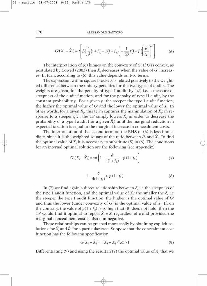
(6)

The interpretation of (6) hinges on the convexity of G. If G is convex, aspostulated by Cowell (2003) then Xi decreases when the value of G' increas-es. In turn, according to (6), this value depends on two terms.

The expression within square brackets is related positively to the weight-ed difference between the unitary penalties for the two types of audits. Theweights are given, for the penalty of type I audit, by 1/δ, i.e. a measure ofsteepness of the audit function, and for the penalty of type II audit, by theconstant probability p. For a given p, the steeper the type I audit function,the higher the optimal value of G' and the lower the optimal value of Xi. Inother words, for a given Ri, this term captures the manipulation of Xi: in re-sponse to a steeper q(.), the TP simply lowers Xi in order to decrease theprobability of a type I audit (for a given Ri) until the marginal reduction inexpected taxation is equal to the marginal increase in concealment costs.

The interpretation of the second term on the RHS of (6) is less imme-diate, since it is the weighted square of the ratio between Ri and Xi. To findthe optimal value of Xi it is necessary to substitute (5) in (6). The conditionsfor an internal optimal solution are the following (see Appendix)

(7)

(8)

In (7) we find again a direct relationship between δ, i.e the steepness ofthe type I audit function, and the optimal value of Xi: the smaller the δ, i.ethe steeper the type I audit function, the higher is the optimal value of G'and thus the lower (under convexity of G) is the optimal value of Xi. If, onthe contrary, the value of p(1 + f2) is so high that (8) does not hold, then theTP would find it optimal to report Xi = Xi regardless of δ and provided themarginal concealment cost is also non-negative.

These relationships can be grasped more easily by obtaining explicit so-lutions for Xi and Ri for a particular case. Suppose that the concealment costfunction has the following specification:

(9)

Differentiating (9) and using the result in (7) the optimal value of Xi that we

G X X X Xi i i i( ˆ ) ( ˆ )− = − , >α α 1

1

4 11

12−

+> +δ

( )( )

fp f

G X X

fp fi i'( ˆ )

( )( ) − = −

+− +

τβ δ1

4 11

12

G X X f p f fR

Xi i

i

i

'( ˆ )ˆ

ˆ − = +( ) − +( )

− +( )

τ βδ δβ

τ11 1

111 2 1

2

02 - santoro 28-07-2008 9:55 Pagina 170


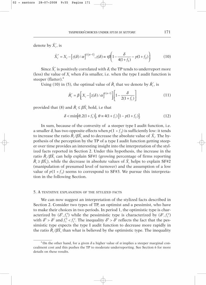
denote by Xi*, is

(10)

Since Xi* is positively correlated with δ, the TP tends to underreport more

(less) the value of Xi when δ is smaller, i.e. when the type I audit function issteeper (flatter).8

Using (10) in (5), the optimal value of Ri that we denote by Ri*, is

(11)

provided that (8) and Ri ≤ βXi hold, i.e that

(12)

In sum, because of the convexity of a steeper type I audit function, i.e.a smaller δ, has two opposite effects when p(1 + f2) is sufficiently low: it tendsto increase the ratio Ri /βXi and to decrease the absolute value of Xi. The hy-pothesis of the perception by the TP of a type I audit function getting steep-er over time provides an interesting insight into the interpretation of the styl-ized facts reported in Section 2. Under this hypothesis, the increase in theratio Ri /βXi can help explain SF#1 (growing percentage of firms reportingRi ≥ βXi), while the decrease in absolute values of Xi helps to explain SF#2(manipulation of presumed level of turnover) and the assumption of a lowvalue of p(1 + f2) seems to correspond to SF#3. We pursue this interpreta-tion in the following Section.

5. A TENTATIVE EXPLANATION OF THE STYLIZED FACTS

We can now suggest an interpretation of the stylized facts described inSection 2. Consider two types of TP, an optimist and a pessimist, who haveto make their choices in two periods. In period 1, the optimistic type is char-acterized by (δ 0, f1

0) while the pessimistic type is characterized by (δ p, f1p)

with δ 0 > δ p and f10 < f1

p. The inequality δ 0 > δ p reflects the fact that the pes-simistic type expects the type I audit function to decrease more rapidly inthe ratio Ri /βXi than what is believed by the optimistic type. The inequality

δ θ θ< , +[ ], ≡ + − +[ ].min ( ) ( ) ( ) 2 1 4 1 1 11 1 2f f p f

ˆ ( )( )

* R X z

fi i= − /[ ]

−+

/ −( )β δ α δα1 1

1

12 1

ˆ ( ) ( )( )

( )*X X z zf

p fi i= − /[ ] , ≡ −+

− +

/ −( )1 1

121

4 11

αδ α δ τβ δ

8 On the other hand, for a given δ a higher value of α implies a steeper marginal con-cealment cost and this pushes the TP to moderate underreporting. See Section 6 for moredetails on these results.

02 - santoro 28-07-2008 9:55 Pagina 171


f10 < f1

p, on the other hand, reflects different expectations about the magni-tude of the penalty, with the pessimistic type expecting a higher penalty (seeSection 2 on the interpretation of the type I penalty as a bargain betweenthe Tax Agency and the TP). Using (5) it is easy to see that if the pessimisticview (with respect to the previous period) is revealed to be the correct one,the optimistic type may be induced to change his expectations and thus hischoices of Ri and of Xi for the second period.

We are now provided with a possible explanation for SF#1 (growing per-centage of firms reporting Ri ≥ βXi) and SF#2 (manipulation of presumed lev-el of turnover): over time, increased pessimism among TPs has persuadedan increasing number of them to expect a “tougher attitude” from the TaxAgency, i.e. a smaller δ and a steeper type I audit function. This, in turn, ac-cording to the results of our model, might have prompted TPs to react by re-ducing Xi given the low value of p(1 + f2) (SF#3), and increase the ratioRi /βXi.

One problem with this explanation is that it is not clear why and howthe pessimistic expectation could have been revealed to be the correct onein the period observed (1998-2004), therefore it is not clear why and how itshould have been endorsed by a growing number of TPs. The most naturalchannel of ex-post revelation of the correct value of δ would be the percent-age of type I audits actually conducted by the Tax Agency. But this percent-age was not revealed until recently and we now know that it has not in-creased over time9 so that it is difficult to make a case for a simple processof rational learning by taxpayers.

The increased pessimism might, however, be the outcome of a coordi-nation game between taxpayers. Suppose that the Tax Agency in a given pe-riod can run a fixed number of audits, possibly defined at the local level. Ifevery TP expects other TPs to report a turnover at least equal to the pre-sumed one, every taxpayer may find it profitable to decrease the probabili-ty of a type I audit by increasing the ratio Ri /βXi.

An alternative channel of the dynamics of δ may be associated with therole of tax practitioners and tax consultants, with particular emphasis onTP’s representatives (see the Introduction) since these organizations act astax consultants for their members. To understand why TP’s representativesmay find it reasonable to suggest ‘pessimism’ we shall recall that TP’s rep-resentatives are actively involved in the elaboration of Sds. This involvementis a source of political power and status, so that it is plausible that TP’s rep-resentatives have made an effort to convince their members of the desir-

9 Data provided by the Tax Agency to the Italian Parliament in June 2007 show that the% of audits has remained approximately constant at around 5% from 1999 to 2002.

02 - santoro 28-07-2008 9:55 Pagina 172


ability of complying with the Sds by reporting Ri = βXi. An emphasis on the‘toughness’ of the Tax Agency, and thus δ = δ p may serve this purpose.10 Thissuggests that the business sectors where the majority of TPs are members ofthe organizations acting as TP’s representatives, should have shown higherrates of compliance with respect to less cohesive sectors. On the other hand,in these highly unionized sectors a stronger lobbying effort displayed by TP’srepresentatives could be associated with a lower value of the threshold βXi

and/or with greater manipulability of X ’s. Although no data on differencesin compliance and thresholds among business sectors have been disclosedso far, the idea that the built-in flexibility of the Sds procedure may led todiscrimination among taxpayers belonging to different sectors has been in-directly acknowledged by the Ministry itself.11 Thanks to the publication ofa tax file reporting microdata on Sds, it should be possible, in the very nearfuture, to test empirically these hypotheses.

6. NUMERICAL SIMULATION

In this Section we present a numerical simulation for the real estate sec-tor. We assume that G(.) is specified as in (9) so that Xi

* and Ri* are given re-

spectively by (10) and (11), under (12). We take the values of β and of Xi fromthe study of sector SG40U (attività immobiliari). More precisely, we identifyXi as the variable ‘square metreage of rented buildings’ since the ‘regionalanalysis’ (analisi di territorialità) indicates that this is the most important re-gressor among those selected in the study. This implies β =7,04 while we as-sume Xi =1000, so that we are applying our approach to a firm which rents1000 squared metres.

For reasons that will shortly become apparent, we first discuss plausi-ble values for the policy variables concerning type II audits, i.e f2 and p.

If we consider that, in general, the probability of a substantial audit (i.eof an audit concerning the accuracy of the data reported by the TP) is around5%, it seems reasonable to assume that

(13) 1 10% p %≤ ≤

10 This pessimism could have gradually spread to the entire population of tax consult-ants through a sort of ‘contagion process’ (Morris, 2000).

11 The Commission for the revision of the Sds (so called Commissione Rey from itsPresident’name)has just released a report that stresses that the arbitrariness in the defini-tion of the ‘consistency criterion’ (see Section 2) may have led to discrimination among dif-ferent economic sectors (and among clusters).

02 - santoro 28-07-2008 9:55 Pagina 173


With regard to f2 we should remember that a type II audit is sanctioned,in general, with unitary sanctions going from 100% to 200% of the tax evad-ed as a consequence of the manipulation (see dlgs 471/1997 article 5, c.4).Thus, in general, we can assume

(14)

We now turn to a discussion of the plausible values of the policy vari-ables concerning type I audit, i.e. f1 and δ .

A type I audit is analysed taking into account the rules of the so-calledaccertamento con adesione. This is a sort of bargaining process between theTP and the Tax Agency which: i) ensures a discount of 25% on the ordinarysanctions (ranging between100% and 200% of the amount due); ii) allowsthe Tax Agency to grant additional ‘discounts’ that may even generate a ‘neg-ative sanction’. In other words, the procedure may end up with a TP payingless than the amount originally due. To take this into account we assume that

(15)

On the other hand, there are reasonable constraints concerning δ :

i) 0 ≤ q ≤ 1ii) Ri

* ≥ 0iii) Xi

* � [0,Xi].

The Appendix shows that, given equations (13), (14) and (15), i), ii) andiii) are jointly equivalent to

(16)

The last variable to be simulated is α. We assumed above that α > 1. Wewill retain the two values of α : α = 1,5 (steep marginal concealment costfunction) and α = 1,1 ( flat marginal concealment cost function).12

To sum up, our simulations for the real estate sector are characterizedby the following features:

i) policy variables are defined by equations (13)-(16); ii) τ = 35%; β = 7,04; Xi = 1000; iii) α either equals 1,1 (flat marginal concealment cost) or 1,5 (steep mar-

ginal concealment cost).

1 2 1 1≤ ≤ +δ ( )f

− , ≤ ≤0 1 11f

1 22≤ ≤f

12 Although these values are similar they produce remarkable differences in equilibri-um values, as we shall see.

02 - santoro 28-07-2008 9:55 Pagina 174


To obtain policy insights we consider two scenarios.

i) a scenario in which p and f2 are given while f1 and δ vary such that theresulting picture is close to the period 1998-2004, which we call the ‘pastscenario’;

ii) a scenario in which f1 and δ are given while p and f2 vary such that theresulting picture resembles the period beginning 2006, which we call the‘future scenario’. To characterize the ‘past scenario’ we need to consider that until 2004

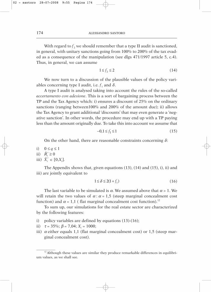
the probability of type II audits was very low. No specific monitoring activ-ity on the values of Xi’s reported by taxpayers was either announced orplanned by the Tax Agency until 2004. Therefore, for the purposes of the ‘pastscenario’, we can assume that p = 1%. Regarding f2, we assume only an in-termediate value, i.e f2 = 1,5. As a consequence in the ‘past scenario’ we havep(1 + f2) = 2,5%.

The values of Ri*, for the case of a steep marginal concealment cost

(α = 1,5) are reported in Table 3 for different values of δ and of f1. Table 3 outlines the standard picture.13 In policy terms, expected rev-

enues can be raised by increasing either the probability of a type I audit orassociated sanctions. As a consequence, the maximum revenue (5.270 euros)

13 Note that, to simplify results, we have taken δ = 1,8 as the maximum value since wehave min(2(1 + f1)) = 1,8. In theory higher values of δ would be admissible for all f1 > –0,1.

TABLE 3 – Values of Ri* for the case of a steep marginal concealment

cost (α = 1,5) in the ‘past scenario’*

δ↓f1→ 1 0,9 0,8 0,7 0,6 0,5 0,4 0,3 0,2 0,1 0 –0,1

1 5.270 5.177 5.075 4.960 4.831 4.685 4.518 4.325 4.100 3.834 3.515 3.125

1,1 5.094 4.993 4.880 4.754 4.612 4.451 4.267 4.055 3.808 3.515 3.164 2.734

1,2 4.919 4.808 4.685 4.547 4.393 4.217 4.017 3.785 3.515 3.196 2.813 2.344

1,3 4.744 4.624 4.490 4.341 4.173 3.983 3.766 3.515 3.222 2.876 2.461 1.954

1,4 4.568 4.439 4.295 4.135 3.954 3.749 3.515 3.245 2.930 2.557 2.110 1.563

1,5 4.393 4.254 4.100 3.928 3.734 3.515 3.264 2.975 2.637 2.238 1.758 1.172

1,6 4.217 4.069 3.905 3.722 3.515 3.281 3.013 2.704 2.344 1.918 1.407 782

1,7 4.042 3.885 3.710 3.515 3.296 3.047 2.762 2.434 2.051 1.599 1.055 391

1,8 3.866 3.700 3.515 3.308 3.076 2.813 2.511 2.164 1.758 1.279 703 0

* Source: author’s simulation for the real estate sector assuming Xi = 1000, β = 7,04, τ = 35%, p(1+f2) = 2,5% andG(.) specified as in (9).

02 - santoro 28-07-2008 9:55 Pagina 175


is obtained when δ = 1 and f1 = 1 (north-west corner of the matrix) and rev-enue is linearly increasing in f1 and decreasing in δ (i.e increasing in thesteepness of q). The ‘growing pessimism’ dynamics referred to in previoussections, i.e. a generalized belief that the Tax Agency is increasing the prob-ability of an audit so that δ is getting lower, should have induced taxpayerswith a steep marginal concealment cost to pay more taxes, even if p(1 + f2)was set at low values.

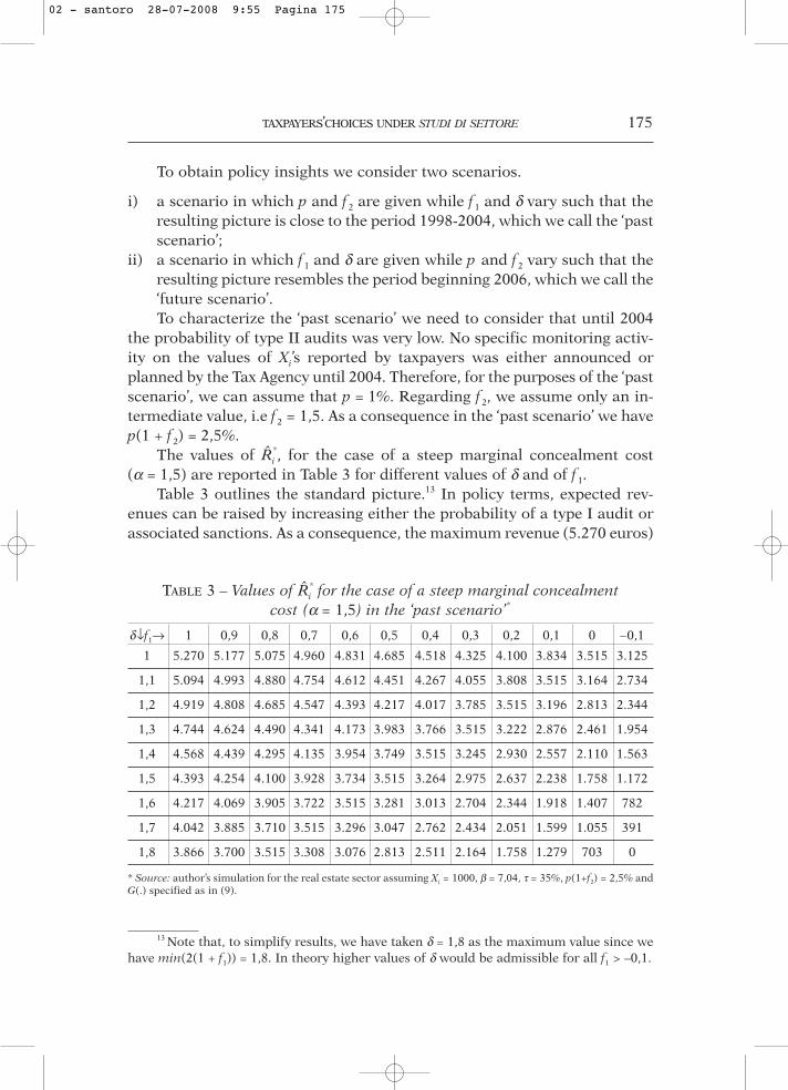
Things change quite dramatically if the marginal concealment cost be-comes flatter, so that α = 1,1.

Various observations can be made. First, the behaviour of Ri

* depicted in Table 4 is neither linear in δ norin f1. We can identify many ‘local maxima’ i.e values of Ri

* which are the max-ima for the row and for the column to which they belong. They are report-ed in italics in Table 4 and they form a sort of diagonal in the matrix. Now,the south-west corner of the matrix is the global maximum (correspondingto approximately 3.193 euros), but all the other local maxima, i.e. numbersin italics along the diagonal, are very close to this value.

In policy terms, this means that to maximize reported revenues whenp(1 + f2) is set at a low value and the marginal concealment cost is flat, theTax Agency should either announce a high probability of audit or a high sanc-tion (i.e adopt a tough attitude in the bargaining process). In other words, wecan say that the two traditional instruments of anti-evasion policies, sanctionsand audits, should not be both increased in this case, i.e when the marginal

TABLE 4 – Values of Ri* for the case of a flat marginal concealment


δ↓f1→ 1 0,9 0,8 0,7 0,6 0,5 0,4 0,3 0,2 0,1 0 –0,1

1 1.974 2.182 2.384 2.577 2.756 2.916 3.048 3.144 3.190 3.173 3.071 2.859

1,1 2.348 2.526 2.693 2.846 2.980 3.087 3.162 3.192 3.167 3.071 2.883 2.580

1,2 2.639 2.784 2.916 3.028 3.116 3.174 3.192 3.162 3.071 2.903 2.640 2.258

1,3 2.857 2.970 3.065 3.138 3.182 3.191 3.158 3.071 2.919 2.688 2.358 1.908

1,4 3.013 3.094 3.154 3.187 3.189 3.153 3.071 2.932 2.726 2.438 2.051 1.541

1,5 3.116 3.165 3.190 3.187 3.149 3.071 2.944 2.758 2.503 2.165 1.726 1.162

1,6 3.174 3.192 3.184 3.146 3.071 2.953 2.785 2.557 2.258 1.875 1.390 778

1,7 3.193 3.181 3.142 3.071 2.961 2.808 2.602 2.336 1.998 1.575 1.047 390

1,8 3.179 3.139 3.071 2.969 2.827 2.640 2.401 2.100 1.726 1.266 700 0

* Source: author’s simulation for the real estate sector assuming Xi = 1000, β = 7,04, τ = 35%, p(1+f2) = 2,5% andG(.) specified as in (9).

02 - santoro 28-07-2008 9:55 Pagina 176


concealment cost is flat and p(1 + f2) is small. The reason for this is that in-creasing the probability of an audit (or increasing the sanction) has oppo-site effects on Ri

*: it decreases Xi* but it also increases the ratio between Ri

*

and a given βXi*. Therefore an appropriate anti-evasion policy targeted to-

wards taxpayers who can easily manipulate Xi’s (i.e who have flat marginalconcealment cost), under a low value of p(1 + f2) , should be based on a bal-ance between δ and f1, since increasing both may be counterproductive. From a different perspective, the results in Table 4 show that the ‘growingpessimism’ emerging from the analysis in the previous sections, i.e. a gen-eralized belief that the Tax Agency was increasing the probability of an au-dit which was lowering δ, may have produced the reverse effects in terms ofrevenues. Such a dynamic would almost inevitably decrease Ri

* in this case(flat marginal concealment cost and low value of p(1 + f2)) if the value of f1

is high (in the range between 70% and 100%) while the reverse would be trueif f1 were low or negative. In other words, increased pessimism may have re-duced the taxes paid by TPs who at the same time believed that the TaxAgency was maintaining a tough stance in the bargaining process generat-ing f1. However, it might also have worked to increase the taxes paid by thosewho believed that a small f1 would emerge.

To sum things up, the ‘past scenario’ suggests that the seemingly disap-pointing results of the Sds in terms of revenues (see Pisani, 2004, Santoro2006) may depend, at least in part, on the fact that many TPs who were ina position to easily manipulate Xi’s have believed that the probability of atype I audit was increasing and that the Tax Agency was adopting a toughstance in the bargaining process generating f1.

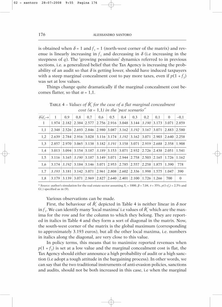
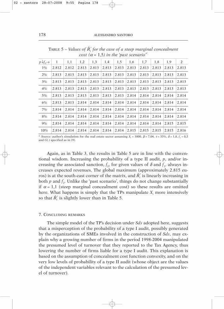
Scenario 2, where p and f2 can vary while f1 and δ are fixed, can be char-acterized to describe the period that beginning 2006. The 2007 budget lawincluded a specific rule for the application of f2 to the case of manipulationof Xi’s and a special type II audit campaign was announced. This may havecaused the values of both p and of f2 to increase. On the other hand, the TaxAgency has revealed that the probability of a type I audit is not particularlyhigh and has given a number of signals that local taxation offices will be like-ly to be fairly lenient in the bargaining process leading to f1. To put thesechanges into the context of our framework, let us suppose that δ = 1,8 andthat f1 = 0,5. Finally, measures were adopted to make the manipulation of Xi’smore difficult and thus more costly.14 In Table 5 we report values of Ri

* forthe case α = 1,5 (flat marginal concealment cost).

14 We refer here to indicatori di normalità economica (economic normality indicators)whose purpose is, for example, to detect taxpayers altering the values of the cost of inven-tories and of the values of capital goods.

02 - santoro 28-07-2008 9:55 Pagina 177


Again, as in Table 3, the results in Table 5 are in line with the conven-tional wisdom. Increasing the probability of a type II audit, p, and/or in-creasing the associated sanction, f2, for given values of δ and f1, always in-creases expected revenues. The global maximum (approximately 2.815 eu-ros) is at the south-east corner of the matrix, and Ri

* is linearly increasing inboth p and f2. Unlike the ‘past scenario’, things do not change substantiallyif α = 1,1 (steep marginal concealment cost) so these results are omittedhere. What happens is simply that the TPs manipulate Xi more intensivelyso that Ri

* is slightly lower than in Table 5.

7. CONCLUDING REMARKS

The simple model of the TP’s decision under Sds adopted here, suggeststhat a misperception of the probability of a type I audit, possibly generatedby the organizations of SMEs involved in the construction of Sds, may ex-plain why a growing number of firms in the period 1998-2004 manipulatedthe presumed level of turnover that they reported to the Tax Agency, thuslowering the number of firms liable for a type I audit. This explanation isbased on the assumption of concealment cost function convexity, and on thevery low levels of probability of a type II audit (whose object are the valuesof the independent variables relevant to the calculation of the presumed lev-el of turnover).

TABLE 5 – Values of Ri* for the case of a steep marginal concealment


p↓f2→ 1 1,1 1,2 1,3 1,4 1,5 1,6 1,7 1,8 1,9 2

1% 2.812 2.812 2.813 2.813 2.813 2.813 2.813 2.813 2.813 2.813 2.813

2% 2.813 2.813 2.813 2.813 2.813 2.813 2.813 2.813 2.813 2.813 2.813

3% 2.813 2.813 2.813 2.813 2.813 2.813 2.813 2.813 2.813 2.813 2.813

4% 2.813 2.813 2.813 2.813 2.813 2.813 2.813 2.813 2.813 2.813 2.813

5% 2.813 2.813 2.813 2.813 2.813 2.813 2.814 2.814 2.814 2.814 2.814

6% 2.813 2.813 2.814 2.814 2.814 2.814 2.814 2.814 2.814 2.814 2.814

7% 2.814 2.814 2.814 2.814 2.814 2.814 2.814 2.814 2.814 2.814 2.814

8% 2.814 2.814 2.814 2.814 2.814 2.814 2.814 2.814 2.814 2.814 2.814

9% 2.814 2.814 2.814 2.814 2.814 2.814 2.814 2.814 2.814 2.815 2.815

10% 2.814 2.814 2.814 2.814 2.814 2.814 2.815 2.815 2.815 2.815 2.816

* Source: author’s simulation for the real estate sector assuming Xi = 1000, β = 7,04, τ = 35%, δ = 1,8, f1 = 0,5and G(.) specified as in (9).

02 - santoro 28-07-2008 9:55 Pagina 178


Since misperception is a market failure, the first, obvious, policy pre-scription would be to give TPs a ‘correct perception’ of the risk by means ofan appropriate auditing policy. Is a policy where the Tax Agency adopts a“tough” stance, the most appropriate? Our model suggests that it may notbe. We have shown, in particular, that the seemingly disappointing resultsof the Sds in terms of revenues (see Pisani, 2004, Santoro 2006) may depend,at least in part, on the fact that many TPs in a position to easily manipulateXi’s believed that the probability of a type I audit was increasing and/or thatthe Tax Agency was taking a tough line in the bargaining process generatingthe penalty f1.

This result is conditional upon the very low probability of a type II au-dit. Increasing the probabilities of and possibly also the sanctions related totype II audits would change the picture quite dramatically, reducing thescope for the manipulation of Xi. It is difficult to understand why such aseemingly simple policy was not implemented until recently. The answerdoes not seem to be related to the legal and institutional features of this typeof audit. As we have seen, there is a legal framework on which type II auditscan be based, and a special type of audit (accesso breve) exists, which is par-ticularly suitable. One explanation is related to the nature of Sds as a polit-ical compromise: the Tax Agency was somehow persuaded that the true val-ues of the independent variables would be spontaneously revealed based onthe fact that the TPs’ representatives were involved in the elaboration of Sds.This belief, however, is not consistent with the evidence. The 2007 ItalianBudget Law seems to be moving along new lines. On the one hand, it intro-duces new parameters (so-called indicatori di normalità economica) whichcan be seen as an attempt to make it more difficult (costly) to manipulate X.On the other hand, it dictates a sharp increase in the number of both type Iand type II audits. It will be interesting to watch the outcome of these poli-cies in future years.

Another, less obvious, policy prescription arising from our analysis isthat the type I audit policy and thus the value of δ should vary according tothe behaviour of the marginal concealment cost function. The marginal con-cealment cost is likely to be positively related to the size of the firm sincebigger (in relative terms) companies need accurate accounting for internalauditing, and to the degree of ‘aversion to evasion’ in the sector/region inwhich the firm operates. The nature of the variable X may also matter sincethere are some variables that are more easy to manipulate than others (usu-ally accounting variables, and costs, which are easier to manipulate thanstructural variables, especially tangibles). There are, or were, lines of evolu-tion within the Sds that try, or tried, to take similar factors into account. Forexample, until recently, the rules under which corporations were audited

02 - santoro 28-07-2008 9:55 Pagina 179


were different from those applied to unincorporated firms which usuallyadopt a simplified accounting regime. Also, in the immediate future the roleof local differences will be heightened.

The most promising lines of future research are mainly empirical. First,when the data become available, it would be interesting to see whether thehypothesis of inter-sector variability in auditability rates is associated, on theone hand, with different threshold values and, on the other hand, with the‘political strength’ of the TP’s representatives in the sectors involved. Second,it might be possible to evaluate the impact of Sds on the firm structure, es-pecially in sectors where a slight change in Xi may have significant conse-quences in terms of the presumed turnover (e.g. by inducing a firm to shiftfrom one cluster to another).

REFERENCES

AGENZIA DELLE ENTRATE (2007), “Gli effetti dell’applicazione degli studi di set-tore in termini di ampliamento delle basi imponibili”, available athttp://www1.agenziaentrate.it/ufficiostudi.

ANDREONI J. - ERARD B. - FEINSTEIN J. (1998), “Tax Compliance”, Journal ofEconomic Literature, vol. 36(2), 818-860.

ARACHI G. - SANTORO A. (2007) “Tax enforcement for SMEs: Lessons from theItalian Experience?”, Atax-Ejournal of Tax Research, 5(2), 224-242.

COWELL F.A. (2003), “Sticks and Carrots”, DARP Discussion Paper 68, Dis-tributional Analysis and Research Programme, London School of Eco-nomics and Political Science.

MORRIS S. (2000), “Contagion”, Review of Economic Studies, 67, 57-78. MYLES G. (1997), “Public Economics”, Cambridge, Cambridge University

Press. PISANI S. (2004), “Il triathlon degli studi di settore”, available at

http://www1.agenziaentrate.it/ufficiostudi. SANCHEZ I. - SOBEL J. (1993), “Hierarchical design and enforcement of inco-

me tax policies”, Journal of Public Economics, 50, 345-369. SANTORO A. (2006), “Evasione e studi di settore: quali risultati? quali pro-

spettive?”, in Rapporto di finanza pubblica 2006, ed. by Guerra M.C -Zanardi A., Bologna, il Mulino, 297-320.

SCOTCHMER S. (1987), “Audit Classes and Tax Enforcement Policy”, TheAmerican Economic Review, 77(2), 229-233.

02 - santoro 28-07-2008 9:55 Pagina 180


APPENDIX

Note that, given (1) we have

We first show how (5) is derived. Using (1) in (3) we obtain

so that

Note that this is a sufficient condition for a minimum since

We now show how (6) is derived. From (4) we have:

Using (1) we can write:

∂∂

= ⇔ − = −

+ − +

+ + −( )∂∂

= ⇔ − = +

′

′

EP

XG X X

R

Xf p f

R

Xf X R

EP

XG X X f

ii i

i

i

i

i

i i

ii i

ˆ ( ˆ )ˆ

ˆ ( ) ( )

ˆ

ˆ( ) ˆ ˆ

ˆ ( ˆ ) (

01 1

1 1

1

01

1

1 2

2 1

τβδ δ β

δβτ β

τβδ 11 2

1 2 1

1

11 1

1

) ( ))

ˆ

ˆ ( )ˆ

ˆ( ) ˆ ˆ

− +

− + + + −( )∂

p f

R

Xf

R

Xf X R

EP

i

i

i

i

i iτβδ β δβ

τ β

∂∂

= ⇔ − = + − +[ ] + + −( )′ ′EP

XG X X q f p f q f X R

i

i i X i iˆ ( ˆ ) ( ) ( ) ( ) ˆ ˆ0 1 1 11 2 1τβ τ β

∂∂

= + >2

212 1

0EP

R

f

Xi iˆ

( )ˆτ

δβ

∂∂

= ⇔ − + −

+ −( )

=

∂∂

= ⇔ − +

+ + =

EP

Rf

R

X XX R

EP

Rf

R

Xf

i

i

i i

i i

i

i

i

ˆ ( )ˆ

ˆ ˆˆ ˆ

ˆ ( )ˆ

ˆ ( )

0 1 11 1 1

0

0 11

12

1

1

1 1

τδ δ β δβ

β

τδ δβ

τ ττδ

δβτ τ

δ

β δ

11

02

12

1 1

0 12 1

1

1 1

1

( )

ˆ

ˆ

ˆ ( ) ( )

ˆ

ˆ

ˆ ( )

+

∂∂

= ⇔ + = + −

∂∂

= ⇔ = −+

f

EP

R

R

Xf f

EP

R

R

X f

i

i

i

i

i

i

∂∂

= − −

+

− + −( )EP

R

R

Xf

Xf X R

i

i

i i

i iˆ

ˆ

ˆ ( ) ˆ ( ) ˆ ˆτδ δ β δβ

τ β11 1

11

11 1

qX

R X

qR

XR X

Ri

i i

Xi

i

i i

′

′

= − < , ≤

=− > , ≤

10

02

δββ

δββ

ˆˆ ˆ

ˆ

ˆˆ ˆ

02 - santoro 28-07-2008 9:55 Pagina 181


Finally, note that is necessary and sufficient for an optimal Xi when

G is convex since since

To derive (7), let us first rewrite (6) as follows:

Then we substitute (5) in (6) and obtain

Note that to have an internal solution a positive value for the RHS of thisexpression is required, i.e.

G X Xf

p f f

G X Xf

p f

G X X

i i

i i

i i

′

′

′

− = − −+

− + , ≡ +

− = − −+

− + ,

−

( ˆ )( )

( ) ( )

( ˆ )( )

( )

( ˆ

Ψ Ψ Ψ

Ψ

βββ δ τβ τ

δ

β δ τβ

2

2

12 1

2

12

12 1

11

1

1 12 1

1

))( ) ( )

( )

( ˆ )( ) ( )

( )

( ˆ )

= − ++

−+

− + ,

− =+

−+

− + ,

− =

′

′

Ψ

Ψ

β δ δ τβ

β δ δ τβ

τβ

1 14 1 1

1

1 4 11

2

12

12

1

2

12 2

f fp f

G X Xf f

p f

G X X

i i

i i 114 1

11

2−+

− +

δ( )

( )f

p f

G X X

R

Xp f fi i

i

i

′ − = −

− + , ≡ +( ˆ )

ˆ

ˆ ( ) ( )Ψ Ψ Ψββ

τβ τδ

2

2 111

1

∂∂

= +

+ − >

2

2 1

22

11

0EP

Xf

R

X XG X X

i

i

i i

"i iˆ

( )ˆ

ˆ ˆ ( ˆ )δβ

τ

∂∂

=EPXiˆ 0

∂∂

= ⇔ − = −

+ − +

+ + −( )∂∂

= ⇔ − = +

′

′

EP

XG X X

R

Xf p f

R

Xf X R

EP

XG X X f

ii i

i

i

i

i

i i

ii i

ˆ ( ˆ )ˆ

ˆ ( ) ( )

ˆ

ˆ( ) ˆ ˆ

ˆ ( ˆ ) (

01 1

1 1

1

01

1

1 2

2 1

τβδ δ β

δβτ β

τβδ 11 2

1 2 1

1 2

1

1

11 1

01

1 1

11

) ( )

ˆ

ˆ ( )ˆ

ˆ( ) ˆ ˆ

ˆ ( ˆ ) ( ) ( )

( )

− +

− + + + −( )∂∂

= ⇔ − = + − +

+ + −

′

p f

R

Xf

R

Xf X R

EP

XG X X f p f

f

i

i

i

i

i i

ii i

τβδ β δβ

τ β

τβδ

τβδδ β

τ βδβ

τδβ

τ βδ δβ

ˆ

ˆ

ˆ ˆ

ˆ

ˆ

ˆ

( ˆ ) ( ) ( ) ( )ˆ

ˆ

R

X

R X

X

R

X

G X X f p f fR

X

i

i

i i

i

i

i

i ii

i

+ −

⇔

− = + − +

− +

′

2

2

1 2 1

2

1

11 1

11

02 - santoro 28-07-2008 9:55 Pagina 182


If the opposite holds, no manipulation is the optimal strategy for the TP

Now, we show that the following set of constraints:

which, adopted in the simulation of Section 6, is equivalent to the followingconstraint on δ:

Given (1) we can write

Now we note that

so that we can write

Now using (5) we note that

and that

so that constraints i) and ii) can be rewritten jointly as

min

ˆ

ˆ ( )R

Xfi

iβδ

= ⇔ ≤ +0 2 1 1

δ

β≥ ⇒ ≤1 1

ˆ

ˆR

Xi

i

0 1 1 1≤ ≤ ⇔ ≤ ≥q

R

Xi

i

ˆ

ˆβδ&

ˆ ˆ minˆ

ˆR XR

Xi i

i

i

≥ ≥[ ]⇔

=0 0 0& β

β

0 1 1 1≤ ≤ ⇔ ≤ ≥ −

.q

R

X

R

Xi

i

i

i

ˆ

ˆ minˆ

ˆβδ

β&

1 2 1 1≤ ≤ +δ ( )f

i) ii)

iii)

0 10

0

≤ ≤≥

∈ ,

qR

X Xi

i i

ˆˆ

p f

fEP

XX X

i

i i( )( ) ˆ

ˆ1 14 1

021

+ > −+

⇒ ∂∂

< ⇒ =δ

1

4 11

12−

+> +δ

( )( )

fp f

02 - santoro 28-07-2008 9:55 Pagina 183


We also know that constraint iii) can be rewritten as follows (see above andequation (8) in text):

Then, we can rewrite constraints i)-iii) jointly as

Finally, we note that

where the last inequality is always verified under(13) and (14).

min ( ) ( ) ( )θ, +[ ] = + ⇔ + <2 1 2 1 1

121 1 2f f p f

1 2 1 4 1 1 11 1 2≤ ≤ , +[ ], ≡ + − +[ ].δ θ θmin ( ) ( ) ( )f f p f

ˆ ( )( )

( ) ( ) ( )X Xf

p f f p fi iδ δ δ∈ , ⇔ −+

≥ + ⇔ ≤ + − +[ ].

0 1

4 11 4 1 1 1

12 1 2

1 2 1 1≤ ≤ +δ ( )f

02 - santoro 28-07-2008 9:55 Pagina 184

taxpayers’choices under studi di settore ... ’choices under studi di settore 163 individual...

Documents