taxation in matching markets - yale university...taxation in matching markets ∗ arnaud †dupuy...
TRANSCRIPT

Taxation in Matching Marketslowast
Arnaud Dupuydagger Alfred GalichonDagger Sonia Jaffesect
Scott Duke Kominerspara
October 2017
Abstract
We analyze the effects of taxation in two-sided matching markets ie markets in which all agents have heterogeneous preferences over potential partners In matching markets taxes can generate inefficiency on the allocative margin by changing who is matched to whom even if the number of workers at each firm is unaffected While the allocative inefficiency of taxation need not be monotonic in the level of the tax when transfers flow in both directions we show that it is weakly increasing in the tax rate for markets in which workers refuse to match without a positive wage
We introduce a renormalization that allows for an equivalence between markets with taxation and markets without taxation but with adjusted match values We use our equivalence to show additional properties of matching markets with taxation and to adapt existing econometric methods to such markets We then estimate the preferences in the college-coach US football matching market and show through simulations of tax reforms that the true deadweight loss can differ dramatically from that measured without accounting for the preference heterogeneity of the matching market
lowastThe authors appreciate the helpful comments of Gary Becker Pierre-Andre Chiappori Raj Chetty David Cutler Steven Durlauf Alexander Frankel Roland Fryer Edward Glaeser Jerry Green Lars Hansen John Hatfield James Heckman Nathaniel Hendren Sabrina Howell Stephanie Hurder Adam Jaffe Peter Klibanoff Fuhito Kojima David Laibson Steven Levitt Robert McCann Stephen Morris Kevin Murphy Yusuke Narita Charles Nathanson Derek Neal Alexandru Nichifor Kathryn Peters Philip Reny Alvin Roth Larry Samuelson Florian Scheuer James Schummer Robert Shimer Aloysius Siow Tayfun Sonmez Rakesh Vohra E Glen Weyl and seminar and conference participants at Aarhus University the Becker Friedman Institute the Fields Institute Harvard University Northwestern University the Paris School of Economics the Rotman School of Management and the University of Wisconsin-Madison
daggerCREA University of Luxembourg and IZA arnauddupuyunilu Dupuy gratefully acknowledges the support of a FNR grant C14SC8337045
DaggerDepartments of Economics and of Mathematics New York University and Fondation Jean-Jacques Laffont Toulouse School of Economics ag133nyuedu Galichon gratefully acknowledges the support of NSF grant DMS-1716489 and ERC grants FP7-295298 FP7-312503 and FP7-337665
sectUniversity of Chicago spjuchicagoedu Jaffe gratefully acknowledges the support of an NSF Graduate Research Fellowship and a Terence M Considine Fellowship in Law and Economics
paraEntrepreneurial Management Unit Harvard Business School Department of Economics Center of Math-ematical Sciences and Applications and Center for Research on Computation and Society Harvard Univer-sity and National Bureau of Economic Research kominersfasharvardedu Kominers gratefully acknowl-edges the support of NSF grants CCF-1216095 and SES-1459912 an NSF Graduate Research Fellowship the Ng Fund of the Harvard Center of Mathematical Sciences and Applications the Harvard Milton Fund a Terence M Considine Fellowship in Law and Economics a Yahoo Key Scientific Challenges Fellowship and an AMSndashSimons Travel Grant
1
Electronic copy available at httpsssrncomabstract=3060746
In addition to highlighting the potential for allocative distortions from taxation our model provides a continuous link between canonical models of matching with and without transfers
Keywords Matching Taxation JEL Classification C78 D3 H2 J3
1 Introduction
Even if high taxes do not cause CEOs to stop working or reduce their hours raising taxes
might affect the sorting of CEOs across firms Taxes reduce large transfers more than small
ones hence high taxes can diminish the extent to which productivity differences are reflected
in post-tax wages Thus under high taxes CEOs may choose the firms they like working
for instead of the ones at which they are most productive An inefficient allocation of CEOs
to firms may not be apparent in the set of workers employed (or the hours that they work)
if there is horizontal heterogeneity in the market ndash that is if CEOs disagree about the
desirability of different jobs and firms disagree about the desirability of CEOs Analogous
re-sorting of workers can happen at all levels of employment so long as there is not perfect
correlation between idiosyncratic job productivity and idiosyncratic tastes
In this paper we analyze the impact of taxation on matching in markets with flexible
preference heterogeneity In matching markets efficiency depends crucially on the assign-
ment of agents to partners ndash not just on the set of agents who are matched in equilibrium
The classical economic intuition that raising taxes always increases equilibrium deadweight
loss holds in markets where agents on one side of the market do not match unless they re-
ceive positive wages however raising taxes can decrease the deadweight loss in fully general
matching markets1 Raising taxes can decrease deadweight loss if it prevents an agent from
making a large enough transfer to an inefficient match partner causing the agent to return
to the efficient match partner he would match with (and receive a transfer from) absent
taxation
In our framework agents have heterogeneous rankings of potential match partners and
can make transfer payments to their partners Transfers may be ldquotaxedrdquo causing some of
each payment to be taken from the agents2 With a proportional tax τ an agent receives
1Most labor markets have wages flowing from firms to workers although there may be internships that workers would pay to get There are other more balanced matching markets where it may be more reason-able to think of transfers flowing in both directions For example most students pay for college but a few are given living stipends or free room and board in order to induce them to attend
2We do not explicitly model the central authority that collects the tax Our welfare analysis focuses on
2
Electronic copy available at httpsssrncomabstract=3060746
fraction (1minusτ) of the amount his partner gives up (see Section 2)3 Taxation lowers the value
of transfers causing agents to prefer match partners that provide higher individual-specific
match values over those offering higher transfers for example with taxation a worker may
switch to a firm he happens to enjoy but at which he is less productive The tax reduces the
firmsrsquo ability to compensate workers for the disutility of jobs where they are more productive
thereby distorting away from efficient matching
The matching distortion we identify differs from the well-known effects of taxation on
intensive and extensive labor supply the matching distortion affects the allocation of workers
to firms without necessarily changing the provision of labor and it is not fully captured by
the elasticity of taxable income Also matching distortions arise even in markets with
frictionless search and thus differ from the well-known effects of search costs on matching
efficiency and of taxation on search behavior4
Although our results are presented in the language of labor markets they also have
implications for other matching markets Some transfers may be non-monetary and therefore
might not be valued equally by givers and receivers colleges may offer free housing to
scholarship students which might cost them more to provide than studentsrsquo willingness to
pay Marriage markets also often have in-kind transfers it may be the case that an agent
may value receiving a gift less than it costs his or her partner (in time and money) to give
it5 Taxation can be reinterpreted as representing the frictions or loss on in-kind transfers
In college admissions and marriage markets positive transfers may flow in both directions
Our non-monotonicity result implies that it is non-trivial to predict the sign of efficiency
consequences of a reduction in transfer frictions
After laying out the general model and theoretical results we turn to a more specific
model for the purposes of estimation We show how the Choo and Siow (2006) framework
for matching with perfect transfers can be adapted to allow for taxation Categorizing agents
by observable type and putting structure on the form of unobserved heterogeneity allows for
the identification of match values from data on matching patterns and wages We apply
this technique to estimate job amenities and productivities of college football coaches We
then use the estimated match values to simulate the market equilibrium under alternative
tax policies We show that the true change in market surplus is not well approximated by
total match value implicitly assuming that the social value of tax revenue equals the private value 3In Appendix D we look at lump sum transfers in which a fixed amount ` is subtracted from transfers 4See for example the work of Blundell et al (1998) and Saez (2004) on how taxation impacts the
intensive margin Meyer (2002) and Saez (2002) on how taxation impacts the extensive margin Mortensen and Pissarides (2001) and Boone and Bovenberg (2002) on search costs and Gentry and Hubbard (2004) and Holzner and Launov (2012) on taxation and search
5A similar idea is modeled by Arcidiacono et al (2011) who treat sexual activity as an imperfect transfer from women to men in the context of adolescent relationships
3
formulas that do not account for the matching nature of the market
Of the vast literature on taxation our work is most closely related to the research on the
effect of taxation on workersrsquo occupational choices and sufficient statistics for deadweight
loss However the prior work on occupational choice (eg Parker (2003) Sheshinski (2003)
Powell and Shan (2012) Lockwood et al (2013)) only reflects part of the matching distor-
tion because it does not model the two-sidedness of the market If workers and firms both
have heterogeneous preferences over match partners then matching distortions can reduce
productivity even without causing an aggregate shift in workers from one firm (or industry)
to another We show that with two-sided heterogeneity measures of deadweight loss based
only on wages (eg Feldstein (1999) and Chetty (2009)) are insufficient
Our approach is also related to the literature on taxation in Roy models (eg Roth-
schild and Scheuer (2012) Boadway et al (1991)) The payoff that a firm in our model
derives from a worker could be thought of the productivity of the worker in that firm or
sector However most Roy models assume that workers earn their marginal product When
preferences are heterogeneous firms may keep some of the productivity surplus ndash if a worker
is more productive at one firm than at any other that one firm need not pay the worker
his full productivity in equilibrium6 Explicitly modeling firms allows for the possibility of
taxation affecting firmsrsquo surplus
Our model of matching with imperfect transfers provides a link between the canonical
models of matching with and without transfers Absent taxation our framework is equiv-
alent to matching with perfect transfers (eg Koopmans and Beckmann (1957) Shapley
and Shubik (1971) Becker (1974)) under 100 taxation it corresponds to the standard
model of matching without transfers (eg Gale and Shapley (1962) Roth (1982)) Thus
the intermediate tax levels we consider introduce a continuum of models between the two
existing well-studied extremes
While prior work has analyzed frameworks that can embed our intermediate transfer
models (Crawford and Knoer (1981) Kelso and Crawford (1982) Quinzii (1984) Hatfield
and Milgrom (2005)) it has focused on the structure of the sets of stable outcomes within
(fixed) models and has not looked at how the efficiency of stable outcomes changes across
transfer models and is therefore unable to analyze the effect of taxation Legros and Newman
(2007) do examine outcome changes across transfer models but they use one-dimensional
agent types and therefore have limited preference heterogeneity
Our econometric framework builds on the seminal paper of Choo and Siow (2006) which
introduced a model of matching with perfect transfers and logit (Gumbel-distributed) het-
6This is true even if firms are price-takers The idiosyncratically high productivity of a given firm means that firmrsquos presence increases the surplus in the market the firm gets to keep some of the marginal surplus
4
erogeneity in preferences in the context of the marriage market7 In applied work on the
marriage market the Choo and Siow (2006) model been used by Chiappori et al (2017) to
measure the changes in the return to marriage by Dupuy and Galichon (2014) to measure
the interaction between personality traits in the formation of marital surplus Empirical as-
signment models have also been used in the labor literature with the notable difference that
unlike in the context of the marriage market where transfers are usually not observed trans-
fers (wages) are typically observed in the labor market Following Tervio (2008) and Gabaix
and Landier (2008) a literature seeks to estimate the productivity of the CEOs based on
data on their compensation and their rank in outcome of the sorting process While most of
these models are unidimensional without unobserved heterogeneity and based on Beckerrsquos
model of positive assortative matching Dupuy and Galichon (2017) have recently proposed
an econometric estimation procedure of matching markets when the matching process is
multidimensional heterogeneity is logit (as in the Choo and Siow (2006) model) and a noisy
measure of transfers is available
The remainder of the paper is organized as follows Section 2 introduces our model
Sections 3 presents the theoretical results Section 4 describes the corresponding econometric
model and results on identification Section 5 describes the data and methods used in
our application it presents the parameter estimates and simulations of counter-factual tax
policies Section 6 concludes All proofs as well as auxiliary results are presented in the
Appendix
2 General Model
We study a two-sided many-to-one matching market with fully heterogeneous preferences
We refer to agents on one side of the market as firms denoted f isin F we refer to agents on
the other side workers denoted w isin W Each agent i isin F cup W derives value from being
matched to agents on the other side of the market We denote these match values by γfD for
the value f isin F obtains from matching with the set of workers D sube W and αfw for the value
w isin W obtains from matching with firm f isin F Without loss of generality we normalize
the value of being unmatched (an agentrsquos reservation value) to 0 setting γff = αww = 0
for all f isin F and w isin W In the labor market context γfD may represent the productivity
of the set of workers D when employed by firm f and αfw may be the utility or disutility
worker w gets from working for f 8
7This framework has extended to general heterogeneity by Galichon and Salanie (2014) and to imperfect transfers by Galichon et al (2017)
8Although it may seem that γfD should be positive and αfw should be negative for our general analysis we do not make sign assumptions That is we allow for the possibility of highly demanded internships and
5
Note that it is possible for workers to disagree about the relative desirabilities of potential
firms and for firms to disagree about the relative values of potential workers For our initial
results we impose no structure on workersrsquo match values and only impose enough structure
on firmsrsquo preferences to ensure the existence of equilibria For example the match values
could be random draws or may result from an underlying utility or production function in
which agents have multi-dimensional types and preferences To ensure existence we assume
that firmsrsquo preferences satisfy the standard Kelso and Crawford (1982)Hatfield and Milgrom
(2005) substitutability condition the availability of new workers cannot make a firm want to
hire a worker it would otherwise reject9
A matching micro is an assignment of agents such that each firm is either matched to itself
(unmatched) or matched to a set of workers who are matched to it Denoting the power set
of W by weierp(W ) a matching is then a mapping micro such that
micro(f) isin (weierp(W ) empty cup f) forallf isin F
micro(w) isin (F cup w) forallw isin W
with w isin micro(f) if and only if micro(w) = f
We allow for the possibility of (at least partial) transfers between matched agents We
denote the transfer from f to w by tfw isin R if f receives a positive transfer from w then
tfw lt 0 A transfer vector t identifies (prospective) transfers between all firmndashworker pairs
not just between those pairs that are matched We also include in the vector t ldquotransfersrdquo tii for all agents i isin F cup W with the understanding that tii = 0 For notational convenience
we denote by tfD the total transfer from firm f to workers in D sube W X tfD equiv tfw
wisinD
In the presence of taxation an agent might not receive an amount equal to that which his
match partner gives up the transfer function ξ(middot) converts an agentrsquos transfer payment into
the amount that agentrsquos partner receives post-tax since we focus on taxes not subsidies
ξ(t) le t In the specific case of proportional taxation the transfer function is
ξτ (tfw) equiv
⎧⎨ ⎩ (1 minus τ)tfw tfw ge 0
1 (1minusτ) tfw tfw lt 0
for counterproductive employees 9Substitutability plays no role in our analysis other than ensuring through appeal to previous work (Kelso
and Crawford (1982)) that equilibria exist Thus we leave the formal discussion of the substitutability condition to Appendix B
6
Figure 1 illustrates the transfer function ξτ (middot) for different tax rates τ
ξ0(tfw)
ξ5(tfw)
ξ9(tfw) tfw
Figure 1 Transfer function ξτ (middot)
An arrangement [micro t] consists of a matching and a transfer vector10 We assume that
agent payoffs are quasi-linear in transfers and that agents only care about their own match
partner(s) With these assumptions the payoffs of arrangement [micro t] for firm f isin F and
worker w isin W are
uf ([micro t]) equiv γfmicro(f) minus tfmicro(f )
uw([micro t]) equiv αmicro(w)w + ξ(tmicro(w)w)
Note that the both the match values and the transfers may be either positive or negative
(The payoff of worker w isin W depends on the transfer function ξ(middot)) As noted above
without loss of generality we normalize the payoff of all unmatched agents to 0
Our analysis focuses on the arrangements that are stable in the sense that no agent
wants to deviate
Definition 1 An arrangement [micro t] is stable given transfer function ξ(middot) if the following
conditions hold
1 Each agent (weakly) prefers his assigned match partner(s) (with the corresponding
transfer(s)) to being unmatched that is
ui([micro t]) ge 0 foralli isin F cup W
10Here were use the term ldquoarrangementrdquo instead of ldquooutcomerdquo for consistency with the matching literature (eg Hatfield et al (2013)) which uses the latter term when the transfer vector only includes transfers between agents who are matched to each other
7
2 Each firm (weakly) prefers its assigned match partners (with the corresponding trans-
fers) to any alternative set of workers (with the corresponding transfers) that is
uf ([micro t]) = γfmicro(f ) minus tfmicro(f) ge γfD minus tfD forallf isin F and D sube W
and each worker (weakly) prefers his assigned match partner (with the corresponding
transfer) to any alternative firm (with the corresponding transfer) that is
uw([micro t]) = αmicro(w)w + ξ(tmicro(w)w) ge αfw + ξ(tfw) forallw isin W and f isin F
We say that a matching micro is stable given transfer function ξ(middot) if there is some transfer vector t such that the arrangement [micro t] is stable given ξ(middot) the transfer vector t is said to support
micro (given ξ(middot)) As we show in Appendix B the stability concept we use is equivalent to the Kelso and
Crawford (1982) competitive equilibrium conceptmdashwhich Kelso and Crawford (1982) showed
is equivalent to the other standard stability concept of matching theory which rules out the
possibility of ldquoblocksrdquo in which groups of agents jointly deviate from the stable outcome
(potentially adjusting transfers)11 The assumption of substitutable preferences ensures that
at least one stable arrangement always exists12
In analyzing stable arrangements we focus on the total value inclusive of tax revenue X X M(micro t) equiv ui(micro(i) t) + tfmicro(f) minus ξ(tfmicro(f))
iisinF cupW f isinF X X X = γfmicro(f) minus tfmicro(f ) + αmicro(w)w + ξ(tfmicro(f)) + tfmicro(f) minus ξ(tfmicro(f))
fisinF wisinW fisinF
= M(micro)
which is just the total match value and depends only on the matching micro not on the supporting
transfer vector t or the transfer function ξ(middot)
Definition 2 We say that a matching micro is efficient if it maximizes total match value among
all possible matchings ie if M(micro) ge M(micro) for all matchings micro 13
11Our stability concept is defined in terms of arrangements the block-based definition is defined only in terms of a matching and the transfers between matched partners Kelso and Crawford (1982) used the term competitive equilibrium for the former concept and used the core to refer to the latter
12Results of Kelso and Crawford (1982) guarantee the existence of a stable arrangement in our framework Details are provided in Appendix B
13An alternative welfare measure would be total agent value ie total match value minus total tax revenue However while government expenditures may not always be valued dollar-for-dollar including government revenue in welfare is typically considered a better approximation than assigning it no value (Mas-Colell et al 1995) Moreover total agent value depends on the transfer vector as there are frequently many transfer
8
Some of our analysis focuses on markets in which workers have nonpositive valuations
for matching so that they will only match if paid positive ldquowagerdquo transfers Formally we
say that a market is a wage market if
αfw le 0 (21)
for all w isin W and f isin F The existence of internships notwithstanding most labor markets
can be reasonably modeled as wage markets
For simplicity we set our illustrative examples in one-to-one matching markets in which
each firm matches to at most one worker for such markets we abuse notation slightly by
only specifying match values for firmndashworker pairs and writing w in place of the set w (eg γfw is denoted γfw)
3 Taxation and Mismatch
In addition to the standard effects of decreasing hours worked or labor market participation
in matching markets taxes can decrease efficiency by creating mismatch in which workers
work for which firms Somewhat surprisingly this mismatch is not necessarily monotonic in
the tax rate as illustrated by the following examples
Example 1 (Non-wage market with linear taxation) We take a simple market with one firm
F = f1 two workers W = w1 w2 and match values as pictured in Figure 2a Worker
w1 receives a high value from matching with f1 Firm f1 is indifferent towards worker w1 and
receives moderate value from matching with w2 Worker w2 has a mild preference for being
unmatched rather than matching with f1 We can think of w1 as an intern who would not
be very productive in working for f1 but would learn a lot w2 represents a normal worker
who is productive but does not like working With this interpretation the tax represents a
proportional income tax ndash which f1 must also pay if the intern w1 bribes him in exchange for
a job
As illustrated in Figure 2b when τ = 1 (or when transfers are not allowed) the only
stable matching micro has micro(f1) = w1 Since micro is efficient matching it is also stable when
τ = 0 as shown in Figure 2c The total match value of micro is M(micro) = 200 Figure 2d shows
that for τ = 8 an inefficient matching micro for which micro(f1) = w2 is stable The inefficient
matching generates a total match value M(micro) = 92 Not only is an inefficient matching
stable under tax τ = 8 but the efficient matching micro is not stable under this tax or any tax
vectors that support a given stable matching total agent value is not typically well-defined even fixing a given stable matching and tax function
9
(b) Matching without Transfers (a) Match Values (τ = 1)
f1
w1
w2
(γf1w1 αm1w1
) = (0200)
(γm1 w2 αm2 w1 ) = (100minus8)
f1
w1
w2
(0 200)
(100minus8)
(d) Matching with Tax (c) Matching with Perfect Transfers (τ = 8)
(τ = 0)
f1
w1
w2
(101 99)
(100minus8) tm1w1
= minus101
tm1 w2 = 0
f1
w1(40 0)
(50 2)tm1w1
= minus40 ξτ(tm1w1
) = minus200
tm1 w2 = 50 ξτ (tm1 w2 ) = 10 w2
Figure 2 Example 1 ndash Non-monotonicity under a proportional tax on transfers
Note Utilities net of transfers are above the lines (firmrsquos workerrsquos) Possible supporting transfers (when applicable) are below the lines Solid lines indicate the stable matching
τ isin (6 9) 14
While Example 1 may appear quite specialized simulations suggest that non-monotonicities
in the total match value of stable matches as a function of τ can be relatively common In
simulations of small markets with utilities drawn independently from a uniform distribution
on [minus5 5] we find that 55 of markets exhibit non-monotonicities (See Appendix C for
details) On average the value drop at a non-monotonicity is 12 of the difference between
the optimal match and the worst match that is stable at any tax rate (for that market)
While our simulations suggest non-monotonicities in the tax rate are not just artifacts of
the example selected they also suggest that non-monotonicities are relatively rare at more
realistic tax rates (τ isin [0 5)) and tend not to persist over large ranges of τ
Although the total match value of stable matchings may decrease when the tax rate
falls an arrangement that is stable under a tax rate τ must improve the payoff of at least
14For that range (100 minus 200(1 minus τ))(1 minus τ ) minus 8 gt 0 so that the maximum f1 can transfer to w2 while still preferring w2 to w1 is sufficient to outweigh the disutility w2 gets from matching to f1 Note that here total agent payoffs (match value minus government revenue) like total match value can be non-monotonic When τ = 1 total agent value is 200 (assuming they do not burn money) when τ = 8 it is 52
10
()
(35minus15)
(0minus125)t = 35 ξτ (t) = 1375
one agent relative to an arrangement that is stable under a tax rate τ gt τ ndash raising the
tax rate cannot lead to a Pareto improvement15 These non-monotonicities can only arise
in non-wage markets so are perhaps more relevant to student-college matching markets or
marriage markets ndash where transfer frictions can act like taxes ndash than to labor markets
Example 2 shows that lower taxes can lower the match value even in wage markets if
taxes are nonlinear
Example 2 (Wage market with piecewise linear taxation) Figure 3a shows the match values
for a market with two firms F = f1 f2 two workers W = w1 w2 Worker w1 (w2) is
fairly productive and receives moderate disutility working for firm f1 (f2) Firm f1 could also
hire worker w2 who is much more productive but dislikes working there more than worker
w1 (There is no surplus from f2 hiring w1)
(b) Transfer functions (a) Match values
(τ1 = 5)
f1
(21 minus10) w1
ξτ (t) τ2 = 5
τ2 = 75
20f2 w2 (21 minus10) t
(c) Matching with Low Tax
(τ1 = 5 τ2 = 5)
f1
f2
w1
(3 1)
(1 0)
(0 5)
t = 32 ξτ (t) = 16
t = 20 ξτ (t) = 10
(d) Matching with High Tax
(τ1 = 5 τ2 = 75)
f1 w1 (0 25)
(0 25)
t = 21 ξτ (t) = 1025
w2 f2 w2 t = 21 ξτ (t) = 105 t = 21 ξτ (t) = 1025
Figure 3 Example 2 ndash Non-monotonicity under a lump sum tax on transfers
Note Utilities net of transfers are above the lines (firmrsquos workerrsquos) Possible supporting transfers (when applicable) are below the lines Solid lines indicate the stable matching
Figure 3b shows the transfer functions There is a marginal tax rate τ1 = 5 on transfers
up to 20 and we consider marginal tax rates of τ2 = 5 75 on the part of the transfer
15See Appendix A and B for the intuition and proof
11
above 20 Fig 3c shows the equilibrium with the lower marginal tax rate of τ2 = 5 The only
stable match is micro(f1) = w2 which gives a match utility of 20 and is inefficient Fig 3d shows
the equilibrium when τ2 = 75 The stable match is micro(f1) = w1 and micro(f2) = f2 which gives
total a total match value of 22 and is efficient Raising the marginal tax rate from τ2 = 5
to τ2 = 75 raises the match utility
Despite our negative results we show that wage markets and proportional taxation to-
gether are sufficient to ensure the match value is (weakly) monotonic in the tax rate Since
payments in wage markets flow from firms to workers any stable matching can be supported
by a non-negative transfer vector16 Thus the transfer function with proportional taxation
ξτ (middot) takes the simpler form
ξτ (tfw) = (1 minus τ)tfw ge 0
Since all positive transfers are paid from firms to workers there cannot be a scenario in
which as in Example 1 when the tax is reduced a firm can transfer enough to get a worker
it prefers (w2) but when the tax falls more a different worker (w1) can ldquobuy backrdquo the
firm17 Moreover as taxes are linear all transfers are equally (proportionally) affected by
the tax rate It cannot be the case as in Example 2 that some transfers are more affected
by the inital tax but others are more affected by the tax increase
Theorem 1 In a wage market with proportional taxation a decrease in taxation (weakly)
increases the total match value of stable matchings That is if in a wage market matching
micro is stable under tax τ matching micro is stable under tax τ and τ lt ˆ τ then
M(micro) ge M(micro)
To prove Theorem 1 we let t ge 0 and t ge 0 be transfer vectors supporting micro and micro
16There may be a supporting transfer vector where some off-path transfers (transfers between unmatched agents) are negative but in that case there is always another supporting transfer vector that replaces those negative transfers with 0s Our results only require the existence of a non-negative supporting transfer vector
17The non-monotonicities described our examples arise from transfers flowing in both directions either simultaneously or across equilibria As transfers are an equilibrium phenomenon requiring that transfers flow in one direction does not directly correspond to conditions on the primitives of the market However the wage market condition we use in Theorem 1 is a sufficient condition on primitives to guarantee that transfers flow in one direction and thus is sufficient to rule out non-monotonicity All the results in this section hold in any market where transfers always (across stable allocations and tax rates) flow in one direction even if it is not a wage market
12
respectively The stability of [micro t] under tax τ implies that
γfmicro(f ) minus tfmicro(f) ge γfmicro(f ) minus tfmicro(f ) and (31)
αmicro(w)w + (1 minus τ)tmicro(w)w ge αmicro(w)w + (1 minus τ)tmicro(w)w (32)
Summing (31) and (32) across agents using the fact that the total transfers paid by all
firms equals the total transfers paid by all workersrsquo match partners18 and regrouping terms
we find that X X M(micro) minus M(micro) = (γfmicro(f) minus γfmicro(f)) + (αmicro(w)w minus αmicro(w)w)
fisinF wisinW X ge τ tfmicro(f) minus tfmicro(f) (33)
fisinF
Equation (33) shows that micro has higher match utility than micro if on average the transfers to
an agentrsquos match partners under micro is greater than the off-path transfer to his partner under
micro Intuitively the match-partner transfers must be larger than the off-paths transfers since
the tax change has a larger effect on larger transfers if we had X tfmicro(f) minus tfmicro(f) lt 0
fisinF
then lowering the tax from τ to τ would increase workersrsquo relative preference for micro over micro
Since micro is stable under the lower tax τ the difference in (33) must thus be positive implying
Theorem 1
Although total match value in wage markets increases as the tax is reduced individual
payoffs may be non-monotonic For example pursuant to a tax decrease a firm f may be
made worse off because his match partner is now able to receive more from some other firm
Firm f might lose his match partner to his competitor even if f rsquos match is unchanged its
total payoff may decrease because it is forced to increase its transfer to compensate for a
competitorrsquos increased offer
31 Renormalizing Utilities
We can renormalize worker utilities in order to express them in pre-tax dollars by defining
1 1 u τ ([micro t]) equiv u([micro t]) = αmicro(w)w + tmicro(w)ww 1 minus τ 1 minus τ
18See Lemma 1 of Appendix B
13
Since the firms care about pre-tax dollars putting workersrsquo match values in pre-tax dollars
makes them easier to aggregate with firmsrsquo match values A post-tax dollar is equivalent to
1minus1 τ pre-tax dollars so workersrsquo match utilities must be divided by (1minusτ ) to lsquopre-taxrsquo values
Workersrsquo relative preferences and therefore the outcomes in the market are unchanged by
the renormalization Since the outcomes are unchanged by the renormalization the matching
market with tax rate τ has the same set of stable matches as a market without taxes that has
match values αfw = 1 αfw and γfw We can then use results from the literature 1minusτ
on matching with transfers to characterize the stable matches
We know that with (perfect) transfers only efficient matches ndash that maximize the sum
of agentsrsquo payoffs ndash are stablethis result no longer holds with a nonzero tax rate because we
are trying to add apples (firmrsquos utilities γfw which are denominated in pre-tax dollars) to
oranges (workerrsquos utilities αfw which are denominated in after-tax dollars) If we express
everything in pre-tax dollars however we get a result parallel to the usual efficiency result
the equilibrium matching maximizes the sum of output measured in a common denomination
Proposition 1 In a wage market with proportional taxation if a matching micro is stable under
tax τ then it is a matching that maximizes the sum of firm utilities plus 1 times the sum 1minusτ
of worker utilities X X1 micro isin arg max γfmicro(f) + αmicro(w)w
micro 1 minus τfisinF wisinW
Additionally P 1 Workersrsquo match value wisinW αmicro(w)w is weakly increasing in the tax rate P 2 Firmsrsquo match value fisinF γfmicro(f) is weakly decreasing in the tax rate
Absent taxation stable matches maximize the sum of match values with equal weight on
firms and workers under taxation stable matches still maximize the sum of match values
but with different weights Taxes decrease the weight put on firmsrsquo preferences because
their ability to express those preferences to workers via wages is decreased As a result the
overall match value of firms decreases with the tax rate Conversely as their preferences
get relatively more weight the overall match value of workers increases with the tax rate
However workers are still better off under lower taxes if they receive sufficiently higher
transfers as to more than compensate for their lower match values
In Appendix A we show some additional features of wage markets
bull If there is more than one tax rate under which two distinct matchings micro and micro are both
stable then micro and micro must have the same total match value M(micro) = M(micro) Moreover
14
firms are indifferent in aggregate between the matchings If micro and micro do not have the
same total match value or firms are not indfferent the only tax rate τ under which
they could both be stable is P wisinW αmicro(w)w minus αmicro(w)w
τ = 1 + P γfmicro(f) minus γfmicro(f)fisinF
bull If two distinct matchings micro and micro are both stable under tax τ then they can be
supported by the same transfer vectors and for any supporting transfer vector all
agents are indifferent between the two allocations (based on Hatfield et al 2013)19
bull There is some τ such that only an efficient matching is stable for τ lt τ
bull If for any τ there are multiple stable arrangements then firms and workers have op-
posing preferences If all firms prefer [micro t] to [micro t] then all workers prefer [micro t] to
[micro t]
In Appendix D we also discuss lump-sum taxation where instead of taking a fixed proportion
of any transfer the tax takes a fixed amount from each transfer Just as under proportional
taxation under lump-sum taxation there a possibility for non-monotonicity and strict wage
markets (where worker match values are strictly negative instead of just non-positive) are
necessary to guarantee monotonicity
32 Implications for Tax Analysis
In addition to causing some workers not to work taxation generates deadweight loss by
changing the matching of workers to firms Thus workersrsquo decisions on where to work affect
firmsrsquo productivity and the opportunities available to other workers These externalities
mean that unlike in the framework of Feldstein (1999) the deadweight loss cannot be
calculated from the change in taxable income20
Using the Feldstein (1999) formula
dDWL dTaxable Income = τ
dτ dτ 19The difference in total match value of the two matches equals the difference in revenue for the two stable
matches for a given supporting transfer vector Unfortunately this equality does not give much traction empirically because as the tax rate changes transfers will change even when the underlying match does not change (so there is no change in total match value) Also even at the tax rate where multiple matches are stable there may be multiple supporting transfer vectors and the revenue between [micro t] and [micro t] does not tell us anything about the difference in total match value between micro and micro
20Chetty (2009) gives other conditions under which the Feldstein (1999) formula does not hold
15
can generate substantial bias in our setting Sometimes when workers switch jobs their
wages drop but the workers like their jobs correspondingly more The change in taxable
income does not capture the fact that workers like their jobs more leading the wage-based
estimate of DWL to be potentially biased upward However there can be increases in wages
that reflect lost profits of the firm rather than increased productivity so the estimate can
also be biased downward
4 Econometric Framework
The preceding results hold for any formulation of match values However they do not tell us
anything about the magnitude of the distortion from taxation as the magnitudes depend on
the distribution of match values in the market To estimate match values so we can simulate
the effect of taxation we now adopt the Choo and Siow (2006) structure assuming that
agents have observable types and limiting the role of unobserved heterogeneity in preferences
We extend the Choo and Siow (2006) framework to account for taxes allowing for tax rates
that vary by individual to accommodate state taxes and different filing statuses We assume
the market is a wage market and the matching is one-to-one21
We assume that each firm f has a (multidimensional) type yf isin Y and each worker has a
(multidimensional) type xw isin X A workerrsquos type may include for example education age
and ability a firmrsquos type may for example include the firmrsquos size or location its technology
and its the management style There are rx workers of type x and my firms of type y
Match values have a systematic component which depends only on the agentsrsquo types and
an additively separable random component that is drawn for each agent-type pair
αfw = αyf xw + σW εyf w
γfw = γyf xw + σF ηfxw
where εyf w and ηfxw are the heterogenous random components of the match utility drawn
from a standard type-I Gumbel distribution
As the number of agents of each type gets large instead of keeping track of which indi-
viduals are matched a matching can be described by the number of matches between each
pair of types which is unaffected by specific draws of εyf w and ηfxw The equilibrium trans-
fers will be also be independent of the random utility draws The set of feasible matchings
21If firms higher more than one worker but their preferences are additively separable then each firm can act as multiple separate firms and the same model applies
16
denoted M(m r) is the set of vectors micro ge 0 such that X microyx le my forally isin Y
xisinXX microyx le rx forallx isin X
yisinY
Transfers are also unaffected by specific draws of εyf w and ηfxw and must be the same for
any agents of the same type tfw = tyf xw
We normalize the systematic utility of being unmatched to 0 for all worker and firm
types and let ε0w and ηf0 also drawn from a standard logit distribution be the random
components for workers and firms respectively Agentsrsquo utilities are
uw = maxmaxαyxw + (1 minus τW )(1 minus τ W )tyxw + σW εyw σW ε0wxw yfy
vf = maxmaxγyf x minus (1 + τF )tyf xw + σF ηfx σF ηf0yfx
where τyW
f is an income tax that varies by firm (state income tax) and τx
W
w is an income tax
that may vary by worker (federal income tax) and τyF f is a payroll tax that may vary by
firm22
41 Renormalization 1minusτ W
Let λW x =
1minus1 τ W and λF = y Using x = xw and y = yf we rescale the amenity and x y 1+τy
F
productivity terms as in Section 31 to define
˜ equiv λW ˜ = λFαyx x αyx γyx y γyx
˜ equiv λW uw ˜ = λF uw x vf y vy
and
˜ equiv ˜ + ˜ = λW + λFφyx αyx γyx x αyx y γyx
Utilities in the fictitious market obtained by the rescaled amenity and productivity terms
are given by
uw = maxmax˜ + ˜ + λW σW εyw x αyxw tyxw x λW σW ε0wy
vf = maxmaxγyf x minus tyf x + λF σF ηfx λF σF ηf0y yx
22For simplicity we do not include payroll taxes that vary by worker but the renormalization we present is still possible
17
where t = (1 minus τy W )t
Without data on unmatched agents we focus on match probabilities and expected payoffs
within the market Using the logit distribution of errors the expected utilities (conditional
on observable types) in our constructed market are
X + ˜
αyx tyx
= λW σW
λW x σ
W
y ax x log exp
X minus ˜γyx tyx by = λF
y σF log exp
λF
σF yx
and we can deduce match frequencies from the logit conditional choice probabilities either
from the workersrsquo side or from the firmsrsquo side αyx+tyx γyxminustyx exp expλWx σ
W λFy σ
F
microyx = rx microyx = my ˜ byexp ax exp
λW σW λF σF x y
If we solve for the match frequencies and the transfers in the system we get respectively 1
λF σF λW σW
λF σF +λW σW αyx + γyx minus ax minus byy y xxmicroyx = my rx exp (41)
λW σW + λF σF x y
and λx
W σW γyx minus by minus λyF σF (αyx minus ax) + λx
W σW λyF σF log(myrx)
tyx = (42)λW σW + λF σF x y
Given pseudo-match values αyx γyxyx and variances σF σW we can solve for the match
probabilities and wages Or given wages and match probabilities we can estimate the match
values and variances
42 Maximum Likelihood
Let the data be a (random sample of the) population of n firm-worker matched pairs indexed
by j isin J For each match j denote by yj the vector of observed attributes of the firm xj
the vector of observed attributes of the worker and ti the noisy measure of the true salary
tyj xj
Without data on unmatched agents one cannot estimate the direct effects of own char-
acteristics on own payoffs ndash the effect of y on γ or the effect of x on α ndash from the matching
pattern or wages So we estimate the effect each partnerrsquos characteristics have on an agentrsquos
18
own match value both directly and interacted with own characteristics We parameterize
the preference of workers for job amenities and firmsrsquo productivity of worker characteristics
linearly as follows
αyx = αyx(A) = x T A0y + AT 1 y + A2
T y(2)
γyx = γyx(Γ) = x T Γ0y + ΓT 1 x + Γ2
T x(2)
where A0 and Γ0 are matrices of coefficients on the cross-terms A1 A2 Γ1 and Γ2 are
vectors of coefficients for the direct effects and v(2) indicates a vector of the same length as
v with each term squared
Preferences and productivity are rescaled to obtain
˜ (A) = λW (A)αyx x αyx
γyx(Γ) = λyF γyx(Γ)
φyx(A Γ) = αyx(A) + γyx(Γ)
The scaling factors of the unobserved heterogeneity are also rescaled ndash from σW to λW x σ
W
and σF to λFy σ
F respectively Hence the distributions of unobserved heterogeneity in the
rescaled economy are fundamentally heteroskedastic when λW x and λF
y vary with x and y
respectively
Our estimation strategy builds on the Dupuy and Galichon (2017) method for maximum
likelihood estimation of amenities and productivities when transfers are observed with noise
Dupuy and Galichon (2017) showed that the log-likelihood function in their context can be
written as the sum of two terms one capturing the likelihood of the observed matches and
one capturing the likelihood of the observed wages
For a given (A Γ) the expected utilities bj (A Γ) and aj (A Γ) are such that for each
worker the sum of their probability of matching with each firm is one and similarly for
workers solution of ⎧ P φyj xj0 (AΓ)minusaj0 minusbj⎪⎪⎨ exp = 1 forallj isin Jj0isinJ λW σW +λF σF x yjj0 P φyj xj (AΓ)minusaj minusbj0⎪⎪⎩ exp = 1 forallj isin Jj0isinJ λW σF xj
σW +λyFj0
with an arbitrarily chosen normalization of ax lowast = 0 The log-likelihood of the observed
match is log L1 (A Γ) = log
Y exp
jisinJ
φyj xj (A Γ) minus aj minus bj λW σW + λF σF xj yj
X =
jisinJ
φyj xj (A Γ) minus aj minus bj λW σW + λF σF xj yj
19
For wages assume that the true (adjusted) wage is observed with error
tj = tyj xj (A Γ c) + (1 minus τyW
j )δj
where c is a constant that accounts for the normalization ax lowast = 0 and the measurement error
δj follows a N (0 s2) distribution independent of (yj xj Zj ) With (42) we see that
λW σW λF σF xj yjtyj xj (A Γ c) = γyj xj minus bj minus αyj xj minus aj + c (43)λW σW + λF σF λW σW + λF σF xj yj xj yj
The likelihood of the observed wages is
n2
2 X tj minus tyj xj (A Γ c) 1 n 2log L2 A Γ c s = minus
2 minus log s
(1 minus τyWj ) 2s 2
j=1
421 Productivity
If available data on firm productivity can also be incorporated yielding a third term in
the expression of the log-likelihood For our application we think that the productivity
measures are more informative of relative team productivity than of absolute productivity
because the teams compete with each other and therefore lose more when the other teams
are more productive Therefore we use only the ordinal ranking of teams
We have a noisy measure of performance Z For notational simplicity we sort matches
by decreasing order of measured performance so Z1 gt Z2 gt Z|J | In addition to the
productivity term γyj xj which affects wages and matching a firmrsquos full productivity is also
directly affected by its own characteristics23 Let cardinal productivity be
Z lowast j = γyj xj + Γ
T Dyj + νi
where νj are drawn from a type-I Gumbel distribution with scaling parameter 1β inde-
pendently of (yj xj δj ) Using γj Tot = γyj xj + ΓD
T yj the probability of the observed ordinal
23These direct effects are not reflected in the matching or wages because if a team is more productive with every potential partner that does not affect the relative probability of matching with one or how much they would pay different partners
20
ranking of teams is
|JY|minus1 γTot γTot Pr (Z lowast gt Z lowast gt gt Z lowast | Γ β) = Pr + νj gt max1 2 n j
jltj0 j + νj
j=1
= |JY|minus1
j=1
βγTot exp jP
βγTot expj0gej j0
The resulting log-likelihood is
log L3 (Γ β) = |J |minus1X
βγTot j
X βγTot minus log exp j0
j=1 j0gej
where the information from the Zs is reflected in the ordering of the js
Finally denoting by θ = (A Γ c s2 β) the vector of parameters of the model we maxi-
mize
log L (θ) = log L1 (θ) + log L2 (θ) + log L3 (θ)
based on the observed yj xj tj Zj
422 Identification Without Wages
If wages are not observed matching patterns generally only identify the sum of the produc-αyx+γyx tivity and amenity of a given match However if tax rates are separately observed σW +σF
and there is sufficient variation in tax rates ndash either separate markets with different tax rates
but the same match surplus function or agents in a single market facing different tax rates αyx γyx ndash then and can be separately identified The intuition is that if agents of type yfσW σF
are more likely to match with agents of type xw in areas with high taxes then more of the αyx surplus from that match must be in σW which gets more weight under higher taxes If
γyx agents are more likely to be matched under low taxes then more of the surplus is in σF
We implicitly use this variation in working with the alternative utilities γ and α but we do
not try to identify the utilities without the wage data
5 Application
We analyze the impact of taxation on the matching market of head coaches and college
football teams in the Division I Football Bowl Subdivision (FBS) of the National Collegiate
Athletic Association (NCAA) in the United States The NCAA FBS market is well-suited
21
to our model for a few reasons First college football coaching is an industry where we
think preference heterogeneity is potentially quite important Coaches have different styles
of coaching which can work very differently for different teams Second there is good data
available not only do we have data on coachesrsquo salaries and characteristics but team perfor-
mance gives us a natural measure of productivity which is not available in most employment
datasets Third the average yearly salary of head coaches in the Division I FBS is about
$18M which is well above the cutoff for the top marginal tax bracket in all states A linear
approximation of taxation of coachesrsquo salaries is therefore justified
Our data allow us to separately estimate coachesrsquo preferences for job amenities and teamsrsquo
productivity the estimates can then be used to simulate the market under alternative tax
policies and compare the deadweight loss of taxation accounting for the matching market
to the deadweight loss estimated ignoring the preference heterogeneity
51 Data
We use data from the 2013 NCAA FBS season the most recent season for which complete
information about teams and coaches was available at the time of the analysis We use
the 115 schools out of 126 in the FBS Division for which wages are publicly available24
The 126 teams are grouped into 10 conferences and include 3 independent teams (Army Air
Force and Navy) Although the conferences are geographically organized there are typically
schools from different states in each conference
511 Sources
We combine data from several sources
The ldquoCoaches Salaries of the Division I FBSrdquo database (USA Today 2013) provides the
salaries of head coaches and their ages and alma maters We gathered information about
the numbers of wins draws and losses of each head coach at the start of each season from
Wikipedia (2013) these allow us to construct measures of coachesrsquo experience and ability
proxied respectively by the numbers of games as head coach and the share of wins both
measured at the start of the season
For team characteristics we get data for each team from the Department of Education
(Office of Postsecondary Education 2013) on the operating expenses and revenues from
sports activities Operating expenses are defined as ldquolodging meals transportation uni-
forms and equipment for coaches team members support staff (including but not limited
24Twenty of the schools are either private or public schools exempted by state law from releasing salary data nevertheless as nine of those schools voluntarily released salaries information salary data are missing for only eleven schools
22
to team managers and trainers) Revenues from sports activities are defined as ldquoall revenues
attributable to intercollegiate athletic activities this includes revenues from appearance guar-
antees and options contributions from alumni and others institutional royalties signage and
other sponsorships sport camps state or other government support student activity fees
ticket and luxury box sales and any other revenues attributable to intercollegiate athletic
activitiesrdquo We also collect a few measures of team performance
bull the numbers of wins losses and ties in the 2013 season (National Collegiate Athletics
Association 2013)
bull the Football Power Index (FPI) which measures the strength of the team as the season
progresses hence allowing us to measure the change between the start and the end of
the season (ESPN 2013)25 and
bull the Football Recruiting Team Ranking (FRTR) which indicates how well a college has
been able to recruit principally under the impulsion of the head coach (247Sports
2013)
Lastly we collect information about the federal and statesrsquo income and payroll tax rates
incurred by both employees and employers from Tax Foundation (2013)
512 Summary
Table (1) presents summary statistics for the variables of interest At the start of the 2013
season the average head coach was 51 years old with 95 games of experience the average
ability amounted to one win every two games In the 2013 season the average yearly salary
of head coaches was approximating $18M although pay differentials across coaches were
quite large as indicated by the relatively large standard deviation (ie $13M) The average
yearly revenues from sports in the division were about $28M while operating expenditures
averaged roughly $34M
52 Estimates of Job Amenities and Productivity
We apply the estimation strategy described in Section 42 to estimate the parameters of
the model Considering age experience and ability and revenues from sports and operating
expenses as the relevant attributes of coaches and teams respectively we obtain estimates
of the direct effects of coachesrsquo and teamsrsquo attributes as well as their interaction on both
25According to ESPN (2013) the FPI ldquois a measure of team strength that is meant to be the best predictor of a teamrsquos performance going forward for the rest of the season FPI represents how many points above or below average a team isrdquo
23
job amenities and productivity Note that all variables are standardized such that each
coefficient can be interpreted in terms of standard deviations of the associated variables
Furthermore using information about coachesrsquo alma maters allows us to estimate the job
amenity and productivity effects of coaching onersquos alma mater team We set σW = 0395
and σF = 001 for the remainder of the analysis these values were selected by performing
a grid search and retaining the pair of parameters yielding the largest maximum likelihood
value while limiting negative wage predictions to a maximum mass of 5 for each team26
Our estimation strategy fits observed wages well (R2 = 078) and fits the performance
ranking moderately well (McFadden pseudo-R2 = 006)27 Table (2) presents estimates for
the direct and interacted effects of school and coach characteristics on job amenities and
productivity For job amenities we find unsurprisingly that coaches have a substantial
willingness-to-pay ndash about one standard deviation of wages ndash for coaching their alma maters
($114M significant at 1) Coaches also prefer heading teams with lower revenues from
sports A one standard deviation increase in revenues from sports decreases the average
amount coaches like working for a team by $630K However this effect is mitigated by
coachesrsquo experience an one standard deviation increase in a coachrsquos experience attenuates
this effect by $170K (significant at 5) We interpret the effect of revenues from sports as
reflecting the impact of higher pressure on the coachrsquos shoulders since revenues from sports
are (partly) resulting from higher recognition and support from the fans (appearances con-
tributions from alumni and others signage and other sponsorships sport camps ticket and
luxury box sales) Our results also show that abler and younger head coaches prefer teams
with larger operating expenses Head coaches with ability one standard deviation above
average (one standard deviation younger than average) derive an additional job enjoyment
worth $260K (resp $210K) when heading a team with operating expenses one standard
deviation above average
Regarding teamsrsquo productivity as presented in the lower part of Table (2) two important
results are worth noting First coaching onersquos alma mater also increases productivity but
the effect is only $180K (significant at 5) much smaller than the effect on job amenities
Second after controlling for the operating budget revenues from sports only increase pro-
ductivity for high-ability coaches With an average coach a one standard deviation increase
in sports revenues decreases productivity by $180K but with a coach whose ability is one
26For a wide range of values of σW and σF the model predicts observed wages very well with an R2 gt 07 and no negative wages for observed coach-team pairs However negative wages do occur for other pairs ie out-of-sample coach-team pairs depending on the values of σW and σF
27Note that we account for the fact that the ranking of teams at the bottom of the performance distribution is noisy and hence difficult to predict We do so by modifying the likelihood function such that only the ranking of the best 15 teams is considered informative hence assuming the ranking beyond the 15-th place is as good as random (see eg Fok et al (2012))
24
standard deviation above the mean the same increase in sport revenues increases produc-
tivity by $60K = 240 minus 180 Our result is in line with our interpretation of revenues from
sports as reflecting pressure put on the team and the coach suggesting that higher pressure
can only be dealt with by high ability coaches
53 Simulations
We can use our estimated parameters to calculate the equilibrium match probabilities and
wages and hence social welfare under alternative tax policies Note however that the
equilibrium wages depend on how agents split the surplus gained or lost from the change
in tax If coaches have the bargaining power then the firmsrsquo outside options determine the
overall wage level in the market meaning that wages for a given match will not change a
lot when the tax rate changes though the probability of matches with high or low wages
will change Conversely if firms have most of the bargaining power then coachesrsquo outside
options determine the overall wage levels As taxes decrease there will be a corresponding
decrease in the overall wage level to keep the post-tax wages mostly unchanged
Unfortunately we do not observe unmatched agents and therefore cannot estimate the
relative bargaining power of the two sides of the market Instead we consider four different
alternative assumptions about how the bargaining power is distributed between the two
sides of the market and derive ndash for each of these alternatives ndash the associated equilibrium
wages at each tax rate The first two alternatives correspond to the extreme points of the
distribution of bargaining power met when either side of the market has no power The
other two alternatives are intermediate points The first intermediate alternative simply
corresponds to an equal distribution of power resulting in a 50-50 split of surplus For the
second intermediate case we note that it is less ldquoefficientrdquo from the perspective of a worker-
firm pair to shift surplus to workers because doing so increases the tax burden we calculate
wages based on an efficiency-weighted split of the surplus between workers and firms28
For each tax rate the equilibrium match probabilities and wages allow one to calculate
welfare and also tax revenue As we vary the tax rate we calculate both the mechanical
change in revenue XX microyxtyxΔτ
y x
28If t1 is the transfer that keeps the average coachesrsquo payoff fixed (teams have all the bargaining power) and t (1minusτ )2 +t
t2 is the transfer that keeps the average teamsrsquo payoff fixed the efficiency weighted transfer is t = 1 2
(1minusτ )2+1
25
and the change in revenue resulting from changes in the match patterns and wages XX 0 0 τ microyxtyx minus microyxt yx (51)
y x
In models of non-matching labor markets (51) is a measure of deadweight loss (DWL)
from the incremental tax increase (see Feldstein (1999) and the discussion in Section 32)
We compare the wage-based measure of DWL from (51) to the actual DWL Note that
since the measure of DWL depends on wages and wages are obtained using four alternative
distributions of bargaining power we therefore have four different measures of DWL to
compare to the true value
531 Federal Top Tax Rate and State Taxes
We first study the effect of varying the federal top tax rate on welfare over the range (0 5)
which contains the 2013 value ie 0419529 The results are presented in Figures 4 and
5 Figure 4 shows the true DWL and three measures of the DWL estimated from wage
changes namely the measure obtained when firms have all the bargaining power the measure
obtained when firms and workers split the surplus 50-50 and the measure obtained under
the efficiency-weighted split of surplus For the three alternative distributions of bargaining
power we consider wages are increasing when taxes increase causing the DWL estimated
from wage changes to be of the wrong sign The wage-based measures of DWL ignore changes
in firm surplus when firmsrsquo have bargaining power their surplus is decreasing in the tax
rate which is not reflected in the three wage-based measures of DWL As shown in Figure
5a the DWL estimated from wage changes under the assumption that coaches have all of
the bargaining power is a more reasonable estimate of the true DWL In that case the wage
for a given match does not change much with the tax rate since it is pinned down by firmsrsquo
outside options As a result wage changes largely reflect workers moving to jobs at which
they are less productive30 However the amenities at those jobs are higher which is not
reflected in the wage thus the estimate of DWL from wage changes generally over-estimates
the true DWL from a tax increase The relationship between the two is different for high
tax rates because of interactions with state taxes Figure 5b graphs the difference between
the true and the DWL estimated from wage changes as a fraction of the true value With
state taxes set to 0 the wage-based estimate of DWL is always more negative than the true
value In contrast with observed state taxes the relationship flips for high tax rates
29The 4195 rate includes federal payroll taxes 30If we do not account for the change in match probabilities increasing the tax causes a very slight increase
in average wage
26
We next study the effect of varying state taxes on welfare We do so by varying the
average level of state taxes both with taxes varying in proportion to their observed levels
and with tax equalized across states With equalized taxes the effect of varying the average
tax level on total welfare is similar to the federal taxes case studied earlier With variation
in taxes across states a proportional increase in tax rates actually leads to an increase in
the (tax-weighted) average wage so the DWL estimated from wage changes are again of the
wrong sign for a large range of tax rates
With variation in state taxes as the average tax level increases coaches can substitute
towards jobs in states with lower tax rates rather than just jobs with higher amenities We
investigate the incidence of this substitution effect by looking at changes in the αmiddotmiddot and γmiddotmiddot values separately Figure 6 shows the total (systematic) productivity XX
microyxγyx y x
and total (systematic) amenities XX microyxαyx
y x
for different average tax rates for the equalized state taxes scenario and the unequal taxes
across states scenario As expected with equalized state taxes we find that amenities are
increasing and productivities are decreasing in the tax rate However with variation in taxes
across states the amenities actually decrease as the tax rates increase (proportionally) the
total productivity falls but to a lower extent than under equalized taxes Productive coaches
substitute towards jobs in states with lower tax rates rather than just jobs with higher
amenities
The potential for substitution across states raises the question of the welfare and revenue
effects of equalizing state taxes To answer this question Figure 7 plots welfare and revenue
relative to the baseline levels for mean tax rates going from 0 (high welfare low revenue)
to the observed mean of 48 for equalized and unequalized taxes The line for equalized
tax rates (dashed line) is down and to the left of the line for tax rates proportional to their
observed levels (sold line) Equalizing tax rates across states for the observed average level
of taxes both lowers revenue and lowers welfare
532 Thresholds and Inframarginal Rates
We next use simulations to look at the effect of varying the federal tax bracket thresholds
and inframarginal tax rates on welfare these exercises require that we account for the fact
27
that the observed federal tax schedule is piecewise linear rather than linear In Appendix
A4 we describe how the convexity of a piecewise linear progressive tax schedule allows a
simple extension of the linear model Intuitively one can think of the htransfer post-tax
transferi pairs that are feasible under a piecewise linear tax as the intersection of the pairs
that are feasible under each of the underlying linear taxes albeit after adjusting the utilities
to account for the fact that the linear schedules for the higher brackets do not intersect the
origin As a result rather than solving for the individual expected utilities (b and a) such that each agentrsquos match probabilities sum to 1 we find the expected utilities such that
the minimum probability across each tax bracket sums to 1
We first study the effect on welfare and revenue of varying the inframarginal tax rate with
piecewise linear taxation When changing the inframarginal tax rate whether the coaches
or teams are the residual claimants to additional surplus affects not only the revenue but
also the welfare Lowering the inframarginal tax rate increases post-tax wages so when
coachesrsquo utility is kept constant there must be an accompanying decrease in the overall
wage level The overall decrease in wages lowers the marginal tax rates for some coaches and
teams leading to an increase in efficiency When teamsrsquo utility is kept constant wages for a
given match do not change systematically or by very much so there is no secondary effect of
overall wage levels on efficiency As a consequence welfare is more sharply decreasing in the
inframarginal tax rate when coaches utility is held constant than when teamsrsquo utility is held
constant as shown in Figure 8a Since wages are increasing in the tax rate when coaches
utility is fixed revenue also increases more quickly in the tax rate as depicted in Figure 8b
Comparing the scales between Figure 8a and Figure 8b we note that the differences in social
welfare across different inframarginal tax rates are very small relative to the differences in
revenue
Finally we can also vary the threshold for the top tax bracket31 The difference in the
tax rate above and below the threshold is 66 percentage points Figure 9 shows welfare
(Figure 9a) and revenue (Figure 9b) as the threshold for the top bracket moves between
$200k and $600k Again and for the same reasons both are more affected by the threshold
when coachesrsquo utility is held fixed than when teamsrsquo utility is held fixed
6 Conclusion
This paper investigates the incidence of taxation in matching markets both theoretically and
empirically On the theoretical side we show through examples and numerical simulations
31Since the tax bracket starts at $400k with a tax rate of 4195 and the bracket below that starts at $398k with a tax rate of 3735 we remove the second-from-the-top bracket
28
that in general the total match value of stable matchings may not vary monotonically as
taxation increases We then show three important positive results for markets that are wage
markets under proportional taxation First as proportional taxes decrease the total match
value of stable matchings (weakly) increases Second while in the absence of taxation
stable matches maximize the sum of match values of workers and firms with unit weights
for workers and firms with tax rate τgt 0 stable matches still maximize the sum of match
values of workers and firms but with respective weights 1 and (1 minus τ) Third workersrsquo
match values are weakly increasing in the tax rate whereas firmsrsquo match values are weakly
decreasing in the tax rate
Using insights from the second result above we adopt the Choo and Siow (2006) approach
on renormalized utilities to account for the linear taxation Since the renormalization also
applies to the random components of the utilities the distributions of unobserved hetero-
geneity are fundamentally heteroskedastic as soon as taxation varies with observed types x
and y We therefore adapt the Dupuy and Galichon (2017) maximum likelihood estimator
of amenities and productivities when transfers are observed with noise to allow for this het-
eroskedasticity Finally we extend the maximum likelihood estimator to the case in which
noisy measures of firm productivity are also observed
We use our estimation strategy to study the matching market of head coaches and college
football teams in the Division I Football Bowl Subdivision (FBS) of the National Collegiate
Athletic Association (NCAA) in the United States We estimate that coaches are willing
to give up $114M in order to coach their alma mater team and prefer heading teams with
low pressure to perform although this latter preference is decreasing with coach experience
We also find that teams are $180K more productive when coached by alma mater coaches
meanwhile team productivity decreases with the pressure to perform unless the team is
coached by a high enough ability coach
We perform simulations of the impact of (federal and state) tax policies based on our
estimates Results confirm that wage-based measures of DWL as suggested by Feldstein
(1999) over-estimate the true DWL from a tax increase if wages do not respond to the tax
because these measures miss the higher amenities that workers receive from lower wage jobs
ignore firmsrsquo surplus Simulations also show that a proportional increase in the average level
of state taxes decreases the average workersrsquo amenities because productive coaches substitute
towards jobs in states with lower tax rates rather than just jobs with higher amenities The
substitution effect we observe can have important welfare implications as our results show
equalizing tax rates across states for the observed average level of taxes both lowers tax
revenue and welfare
29
Tables and Figures
Table 1 Summary statistics of coachesrsquo and teamsrsquo attributes
Mean Std Min Max Coaches Age (in years) Experience (games) Ability (winsgame) Salaries (in $M) Coaches at Alma Mater
51 95 051 177 009
8 87 023 130 028
33 0
000 029 0
74 389 091 555 1
Teams Revenues from sports (in $M) Operating expenses (in $M) Performance Principal Component
2802 335 -000
2394 230 135
411 060 -304
11251 1523 365
N= 115
Note Salaries refers to total pay which includes school pay ndash the base salary paid by the university plus other income paid or guaranteed by the university ndash and other pay not guaranteed by the university On average school pay represents 99 of total pay The performance measure is the principal component of a PCA performed on 1) the number of wins in the season 2) the change in FPI index between start and end of season and 3) the FRTR ranking
30
Table 2 Effect of coachesrsquo and teamsrsquo attributes on job amenities and productivity (in $M)
Main effects Revenues from
sports (in $M)
Operating expenses (in $M)
Job Amenities (Alpha) Main effects -063 -011
(007) (007) Age (in years) -009 -021
(009) (009) Experience ( of games) 017 010
(008) (009) Ability (winsgame) 009 026
(010) (009) Alma Mater 113
(014) Productivity (Gamma) Main effects -018 035
(009) (016) Age (in years) -004 -000 016
(005) (007) (009) Experience ( of games) 011 000 -019
(006) (006) (011) Ability (winsgame) 013 024 -010
(007) (011) (012) Alma Mater 018
(009) Scaling performance 721
(324) Salary constant 896
(027)
Note This table reports the estimates of effects the interaction of coach characteristics and team character-istics on team productivity and job amenities measured in millions of dollars All covariates except for Alma Mater are standardized to have a standard deviation of 1 Standard errors calculated from the Hessian of the likelihood are in parentheses Scaling performance refers to the variance of the error in the performance equation (β)
31
Figure 4 Marginal deadweight loss from a 1pp increase in the federal tax
Note This graph shows the deadweight loss (DWL) in millions of dollars from a one percentage point increase in the federal tax rate The botthom line is the true DWL from the simulation and top three lines are the DWL estimated based on the changes in wages under differ three different assumptions about how wages adjust to account for the change in surplus from the change in the tax rate The first holds the coaches utility fixed so any additional surplus goes to the teams The second splits the surplus 50-50 and the last does an efficiency-weighted split of the surplus as described in Section 53 All of the wage-based estimates are of the wrong sign because wages increase to compensate workers for loss from the higher tax rate
32
(a) True and estimated (b) Error in estimate
Figure 5 Marginal deadweight loss from increase in the federal tax
Note This graph shows the deadweight loss (DWL) in millions of dollars from a one percentage point increase in the federal tax rate The solid line shows the true DWL from the simulation and the dashed line shows the DWL estimated based on the changes in wages assuming that coaches have all the bargaining power (where wages change very little in response to changes in the tax rate) The wage-based estimate over estimates the DWL because it does not account for the higher amenities workers receive in matches where they are less productive and paid lower wages
33
Figure 6 Effect of state taxes on amenities (α) and productivity (γ)
Note This graph shows the effect of state tax rates on the total productivity and amenities of the equilibrium match Quantities are in thousand of dollars and relative to baseline levels The mean tax rate is varied from 0 to 048 first keeping taxes proportional to their observed level and then for tax rates equalized across states When taxes vary across states coaches can substitute to states with lower taxes instead of jobs with high amenities so the amenities do not increase with the tax rate as they do when taxes are equalized across states
34
Figure 7 Relationship between welfare and revenue
Note This graph shows the how welfare and revenue co-vary as the state tax rate changes Both quantities are in thousand of dollars and relative to baseline levels The mean tax rate is varied from 0 to 48 first keeping taxes proportional to their observed level and then for tax rates equalized across states For a given revenue welfare is lower when taxes are equalized across states
(a) Welfare (b) Revenue
Figure 8 Effect of the infra-marginal tax rate
Note These graphs shows the effect of changing the inframarginal tax rate on tax revenue and social welfare Quantities are in thousand of dollars and relative to baseline levels The top marginal tax rate is kept constant at 4195 All income below 400k is treated as a single bracket whose tax rate varies from 0 to 4195 The effects on revenue are much larger than those on welfare
35
(a) Welfare (b) Revenue
Figure 9 Effect of the threshold for the top tax bracket
Note These graphs shows the effect of changing the threshold above which the top marginal tax rate of 4195 applies Quantities are in thousand of dollars and relative to baseline levels To make the effect clearer we drop the second from the top bracket so all income below the threshold and above $183 is taxed at 3535 So the change in marginal tax rate at the threshold is 66 The effects on revenue are much larger than those on welfare
36
Appendix
A Additional Theoretical Results
A1 Taxes cannot cause Pareto improvements
Although Example 1 and the simulations show that total match value of stable matchings may decrease when the tax rate falls an arrangement that is stable under a tax rate τ must raise the payoff of at least one agent relative to an arrangement that is stable under a tax rate τ gt τ
Proposition 2 Suppose that [micro t] is stable under tax τ and that [micro t] is stable under tax τ with ˇ τ micro ˇ τ) cannot Pareto dominate [ˆ t] (under tax ˆτ gt ˆ Then [ˇ t] (under tax ˇ micro ˆ τ )32
To see the intuition behind Proposition 2 we consider the case in which τ = 1 and choose t = 0 If [micro t] (under tax τ = 1) Pareto dominates [micro t] (under tax τ) then every firm f isin F (weakly) prefers micro(f) to micro(f) with the transfer tfmicro(f ) 33 But then because [micro t] is stable under tax τ
Pareto Stabilityz| z|γfmicro(f ) ge γfmicro(f) minus tfmicro(f) ge γfmicro(f) minus tfmicro(f)
so every f must be offering a weakly positive transfer to micro(f) under t (that is tfmicro(f) ge 0) An analogous argument shows that each worker w isin W must be offering a weakly positive transfer to micro(w) under t (that is ξτ (tmicro(w)w) le 0) Moreover Pareto dominance implies that at least one firm or worker must be paying a strictly positive transfer But then that agent must pay a strictly positive transfer and receive a weakly positive transfer ndash impossible
A2 The Effect of Very Small Taxes
Unlike in non-matching models of taxation in our setting there is always a nonzero tax that does not generate distortions To find the minimum tax that generates a distoriton let micro be an efficient matching Our results show that if micro is stable under τ then34
M(micro) minus M(micro)τ ge P (A1)
(γfmicro(f) minus γfmicro(f))f isinF
32We say that an arrangement [micro t] under tax τ Pareto dominates arrangement [micro t] under tax τ if
γfmicro(f ) minus tfmicro(f ) ge γfmicro(f) minus tfmicro(f) forallf isin F
αmicro(w)w + ξτ (tmicro(w)w) ge αmicro(w)w + ξτ (tmicro(w)w) forallw isin W
with strict inequality for some i isin F cup W 33Note that under tax τ = 1 an arrangement with transfers of 0 among match partners Pareto dominates
any other arrangement with the same matching Thus the transfers between match partners under [micro t] can be assumed to be 0 Then the comparison between [micro t] (under tax τ = 1) and [micro t] (under tax τ ) amounts to a comparison of agentsrsquo match values under micro and their total utilities under [micro t]
34See Section B6
37
For any inefficient matching micro there is a strictly positive minimum tax τ(micro) at which micro could possibly be stable Since there are finitely many possible matchings we can just take the minimum of this threshold across inefficient matchings
τ lowast = min [τ(micro)] microM(micro)ltM(micro)
For τ lt τ lowast only an efficient matching can be stable35
A3 Multiple matches stable at a given tax rate
Hatfield et al (2013) shows that in markets with perfect transfers if two matches are stable they can be supported by the same transfer vector and all agents are indifferent between the two allocations These results carryover to the case of taxation as summarized in the following proposition
Proposition 3 In a wage market if two matches micro and micro are both stable at tax rate τ then
1 Any transfer vector that supports one match also supports the other
2 For any supporting transfer vector all agents are indifferent between the two alloca-tions
3 The difference in total match value of the two matches equals the difference in revenue for the two stable matches for a given supporting transfer vector
Proof For any stable outcomes micro and micro and a transfer vector t that supports one of the stable matches we can renormalize worker match utilities αfw = 1 αfw and be in a
1minusτ market where the results of Hatfield et al (2013) apply
γfmicro(f ) minus tfmicro(f ) = γfmicro(f) minus tfmicro(f) forallf 1 1
αmicro(w)w + twmicro(w) = αmicro(w)w + tfmicro(w) forallw 1 minus τ 1 minus τ
These equalities hold when we switch back to the original utilities so any supporting transfer vector must support both matches and agents are all indifferent between the two allocations Multiplying the second line by (1 minus τ) and summing across agents gives X X
M(micro) minus M(micro) = τ tfmicro(f ) minus τ tfmicro(f) fisinF fisinF
Unfortunately this result about changes in revenue reflecting changes in value is very limited As the tax rate changes transfers will change even when the underlying match does not change (so there is no change in total match value) Also even at the tax rate
35One caveat is that if there are multiple efficient matchings (all of which are stable when τ = 0) some of them may not be stable in the limit as τ rarr 0
38
where multiple matches are stable there may be multiple supporting transfer vectors and the revenue between [micro t] and [micro t] does not tell us anything about the difference in total match value between micro and micro Similarly results of Kelso and Crawford (1982) and Hatfield and Milgrom (2005) imply
that for any fixed τ if there are multiple stable arrangements then workersrsquo and firmsrsquo interests are opposed If all firms prefer [micro t] to [micro t] then all workers prefer [micro t] to [micro t] Moreover there exists a firm-optimal (worker-pessimal) stable arrangement that the firms weakly prefer to all other stable arrangements and a worker-optimal (firm-pessimal) stable arrangement that all workers weakly prefer More generally
Proposition 4 In a wage market with proportional taxation if two distinct matchings microand micro are both stable under tax τ then X X
αmicro(w)w minus αmicro(w)w = (1 minus τ) γfmicro(f ) minus γfmicro(f ) (A2) wisinW f isinF
Thus if the firms are not indifferent in aggregate between micro and micro then the only tax rate τ under which both micro and micro can be stable is P
αmicro(w)w minus αmicro(w)wτ = 1 + PwisinW (A3)
fisinF γfmicro(f) minus γfmicro(f)
For τ as defined in Equation (A3) to be less than 1 the fraction on the righthand side must be negative so that that firms and workers in aggregate disagree about which matching they prefer In wage markets with proportional taxation where there is generically a unique stable matching this opposition of interests carries over to the set of supporting transfer vectors In order for there to be multiple values of τ at which two given matchings are both stable
both firms and (following (A2)) workers must be indifferent between those two matchings
Corollary 1 In a wage market with proportional taxation if there is more than one tax under which two distinct matchings micro and micro both are stable then M(micro) = M(micro)
Corollary 1 implies that for generic match values there is at most one value of τ at which two matchings micro and micro are both stable since there are finitely many matchings there is a unique stable matching under almost every tax τ
A4 Nonlinear taxes
The wage schedule is in fact progressive and the workerrsquos income is a concave function of the nominal transfer We do not have general theoretical results for non-linear taxes but we can adapt the econometric framework we use to calculate the market equilibrium to the case of piecewise linear taxes Assume that the tax rates on workers are τW 1 lt τW 2 lt lt τW K where τW 1 and τ W K
x x x x x
are respectively the lowest and the top tax rate Tax rate τx W k applies to the income above
tkx where tx 1 = 0 so that if ξxy(tkx) is the post-tax income of a worker of type x earning tkx
39
and working for a firm of type y then k+1 k 1 minus τ W k k+1 kξxy(tx ) = ξxy(tx) + 1 minus τy
W x tx minus tx
More generally the post-tax income of a worker of type x working for a firm of type y and earning tkx is
k 1 minus τW k kξxy(t) = min ξxy(tx) + 1 minus τy W
x t minus t x kisin1K
Hence the systematic utility of a worker x working for a firm of type y with pre-tax income t is
1 minus τW kαk 1 minus τWmin + x (A4)uxy = xy y t kisin1K αk 1 minus τW τW k+1 minus τW k tk+1where α1 = and αk+1 = + x x On the firmrsquos side the xy αxy xy xy y x
systematic utility is still vyx = γyx minus 1 + τy
F t (A5)
Substituting out t from equations (A4) and (A5) one gets 1 minus τ W k γyx minus vyx
uxy = min αxyk + 1 minus τy
W x
kisin1K 1 + τF y
which can be rewritten as 1 minus τW k γyx minus vyx
min αk minus uxy + 1 minus τ W = 0xy y x kisin1K 1 + τF
y
1minusτ W
So letting λW x k = 1
W k (and λFy =
1+τyF as before) we have 1minusτx y ( )
λF
αk ymin xy minus uxy + (γyx minus vyx) = 0
λW kkisin1K x
which is equivalent to ( )λW k(αk x xy minus uxy) + λF
y (γyx minus vyx)min = 0 (A6)
σW λW kkisin1K x + σF λyF
By the log-odds formula we have
microxy microxyσW ln = uxy and σF ln = vxy
microx0 micro0y
where microx0 and micro0y adjust so that each agentrsquos match probabilities sum to 1 After plugging
40
in into expression (A6) we get ⎧⎨ ⎩ λW k(αk + σW + σFln microx0 ) + λF γyx ln micro0y x xy ymicroxy microxy
σW λW k + σF λF x y
⎫⎬ ⎭ = 0min kisin1K
This implies that (λW k(αk + σW + σFln microx0) + λF (γyx ln micro0y)x xy y
σW λW k + σF λF x y
)ln microxy = min
kisin1K
which yields = min Mk (microx0 micro0y)
kisin1K microxy xy
where Wk σF λF Wk σWλx y λ αk +λF γyx x xy y
Wk Wk σW λ +σF λF σWλ +σF λF Wk x y x y σWλ +σF λF
xMk (microx0 micro0y) = micro micro e y xy x0 0y
We use this to solve for the equilibrium microx0 micro0y such that the probabilities for each x and each y sum to 1
B Proofs for Section 2 and Appendix A
B1 Existence of Stable Arrangements amp Equivalence with the Core and Competitive Equilibria
In this section we use results from the literature on matching with contracts to show the existence of stable arrangements in our framework For a given transfer vector t the demand of firm f isin F denoted Df (t) is
Df (t) equiv arg max γfD minus tfD DsubeW
Definition 3 (Kelso and Crawford (1982)) The preferences of firm f isin F are substitutable if for any transfer vectors t and t with t ge t there exists for each D isin Df (t) some D isin Df (t) such that
ˇ = ˇD supe w isin D tfw tfw
That is the preferences of f isin F are substitutable if an increase in the ldquopricesrdquo of some workers cannot decrease demand for the workers whose prices remain unchanged36
Theorem 2 of Kelso and Crawford (1982) shows that under the assumption that all firmsrsquo preferences are substitutable there is an arrangement [micro t] that is strict core in the sense
36Theorem A1 of Hatfield et al (2013) shows that in our setting the Kelso and Crawford (1982) sub-stitutability condition is equivalent to the choice-based substitutability condition of Hatfield and Milgrom (2005) that we describe in the main text the availability of new workers cannot make a firm want to hire a worker it would otherwise reject
41
that37
bull Each agent (weakly) prefers his assigned match partner(s) (with the corresponding transfer(s)) to being unmatched that is
ui([micro t]) ge 0 foralli isin F cup W
bull There does not exist a firm f isin F a set of workers D sube W and a transfer vector tsuch that
γfD minus tfD ge γfmicro(f) minus tfmicro(f) and
αfw + ξ(tfw) ge αmicro(w)w + ξ(tmicro(w)w) forallw isin D
with strict inequality for at least one i isin (f cup D)
The Kelso and Crawford (1982) (p 1487) construction of competitive equilibria from strict core allocations then implies that there is some transfer vector t having tmicro(w)w = tmicro(w)w (for each w isin W ) such that [micro t] is stable in our sense
B2 Total transfers
We use the following Lemma in proving many of the results
Lemma 1 For a given matching micro and transfer vector t the sum of transfers firms pay to their match partners equals the sum of the transfers paid by workersrsquo match partners X X X X X
tfmicro(f ) = tfw = tmicro(w)w le ξ(tmicro(w)w) fisinF fisinF wisinmicro(f) wisinW wisinW
Proof Letting B be the set of firms who are matched at micro and B be the set of workers who are matched at micro we have
micro(f) sube B forallf isin B
micro(w) isin B forallw isin B
37Strictly speaking Kelso and Crawford (1982) have one technical assumption not present in our frame-work they assume that γfw +αfw ge 0 in order to ensure that all workers are matched However examining the Kelso and Crawford (1982) arguments reveals that this extra assumption is not necessary to ensure that a strict core arrangement exists ndash the Kelso and Crawford (1982) salary adjustment processes can be started at some arbitrarily low (negative) salary offer and all of the steps and results of Kelso and Crawford (1982) remain valid with the caveat that some workers may be unmatched at core outcomes
42
We then use the fact that tff = tww = 0 to show that X X X X tfmicro(f) = tfmicro(f) + tfmicro(f) = tfmicro(f)
fisinF fisinB fisinF B f isinB X X X = tfw = tmicro(w)w
fisinB wisinmicro(f) wisinB X X X = tmicro(w)w + tmicro(w)w = tmicro(w)w
wisinB wisinW B wisinW
B3 Proof of Proposition 2
First we show that the arrangements stable under full taxation (τ = 1) cannot Pareto dominate those stable under tax τ lt 1
Claim 1 Suppose that [micro t] is stable under tax τ lt 1 and that [micro t] is stable under tax τ = 1 Then [micro t] (under tax ˇ micro t] (under tax ˆτ = 1) cannot Pareto dominate [ˆ τ lt 1)
Proof As no transfers get through under full taxation an arrangement stable under full tax-ation is most likely to Pareto dominate some other arrangement when all transfers between match partners are 0 Thus we assume that tmicro(w)w = 0 for each w isin W If [micro t] (under full taxation) Pareto dominates [micro t] (under tax τ) then
γfmicro(f ) = γfmicro(f) minus tfmicro(f) ge γfmicro(f) minus tfmicro(f) (B1)
αmicro(w)w = αmicro(w)w + ξτ (tmicro(w)w) ge αmicro(w)w + ξτ (tmicro(w)w) (B2)
with strict inequality for some f or w However stability of [micro t] under tax τ implies that
γfmicro(f ) minus tfmicro(f) ge γfmicro(f ) minus tfmicro(f ) (B3)
αmicro(w)w + ξτ (tmicro(w)w) ge αmicro(w)w + ξτ (tmicro(w)w) (B4)
Combining (B1) and (B3) gives
0 ge minustfmicro(f) (B5)
for each f isin F while combining (B2) and (B4) gives
0 ge ξτ (tmicro(w)w) (B6)
for each w isin W Strict inequality must hold in (B5) or (B6) for some f or w In the first of these cases we have
tf 0 micro(f 0) gt 0
43
for some f 0 isin F hence there exists at least one w isin micro(f 0) for whom
tmicro(w)w gt 0 (B7)
But (B7) contradicts (B6) In the second case we have
0 gt ξτ (tmicro(w0)w0 ) (B8)
for some w0 isin W If we take f = micro(w0) then (B8) and (B6) together imply that X 0 gt tmicro(w)w = tfmicro(f)
wisinmicro(f)
contradicting (B5)
For τ lt 1 ξτ (middot) is strictly increasing and the conclusion of the proposition follows from the following more general result
Proposition 2rsquo Suppose that ξ(middot) is strictly increasing that [micro t] is stable under ξ(middot) and that [micro t] is stable under ξ(middot) with ξ(middot) le ξ(middot) Then [micro t] (under ξ(middot)) cannot Pareto dominate [micro t] (under ξ(middot))38
Proof Pareto dominance of [micro t] (under ξ(middot)) over [micro t] (under ξ(middot)) would imply that
γfmicro(f ) minus tfmicro(f) ge γfmicro(f ) minus tfmicro(f ) (B9)
+ ξ(ˇ + ξ(ˆαmicro(w)w tmicro(w)w) ge αmicro(w)w tmicro(w)w) (B10)
with strict inequality for some f or w However stability of [micro t] under ξ(middot) implies that
γfmicro(f ) minus tfmicro(f) ge γfmicro(f ) minus tfmicro(f ) (B11)
αmicro(w)w + ξ(tmicro(w)w) ge αmicro(w)w + ξ(tmicro(w)w) ge αmicro(w)w + ξ(tmicro(w)w) (B12)
where the second inequality in (B12) follows from the fact that ξ(middot) ge ξ(middot) Combining (B9) and (B11) gives
tfmicro(f) ge tfmicro(f) (B13)
38We say that an arrangement [micro t] (under ξ(middot)) Pareto dominates arrangement [micro t] under (under ξ(middot)) if
γfmicro(f) minus tfmicro(f) ge γfmicro(f) minus tfmicro(f ) forallf isin F
αmicro(w)w + ξ(tmicro(w)w) ge αmicro(w)w + ξ(tmicro(w)w) forallw isin W
with strict inequality for some i isin F cup W
44
for each f isin F while combining (B10) and (B12) gives
ξ(tmicro(w)w) ge ξ(tmicro(w)w)
tmicro(w)w ge tmicro(w)w (B14)
for each w isin W where the second line of (B14) follows from the fact that ξ(middot) is strictly increasing Strict inequality must hold in (B13) or (B14) for some f or w In the first of these cases we have
tf 0 micro(f 0) gt tf 0 ˇ micro(f 0)
for some f 0 isin F hence there exists at least one w isin micro(f 0) for whom
ˆ gt ˇtmicro(w)w tmicro(w)w (B15)
But (B15) contradicts (B14) In the second case we have
tmicro(w0)w0 gt tmicro(w0)w0 (B16)
for some w0 isin W If we take f = micro(w0) then (B16) and (B14) together imply that X X ˇ ˆtmicro(w)w gt tmicro(w)w
wisinmicro(f) wisinmicro(f )
hence we find that
tfmicro(f) gt tfmicro(f )
contradicting (B13)
B4 Proof of Theorem 1
If micro = micro then the theorem is trivially true Thus we consider a wage market in which [micro t] is stable under tax τ [micro t] is stable under tax τ τ gt τ and micro 6= micro The stability conditions for the firms imply that
γfmicro(f ) minus tfmicro(f) ge γfmicro(f ) minus tfmicro(f ) (B17)
γfmicro(f ) minus tfmicro(f) ge γfmicro(f ) minus tfmicro(f ) (B18)
these inequalities together imply that X X tfmicro(f ) minus tfmicro(f) ge tfmicro(f) minus tfmicro(f) (B19)
f isinF fisinF
45
As the market is a wage market we have
ξτ (tmicro(w)w) = (1 minus τ)tmicro(w)w and ξτ (tmicro(w)w) = (1 minus τ)tmicro(w)w
hence the stability conditions for the workers imply that
αmicro(w)w + (1 minus τ)tmicro(w)w ge αmicro(w)w + (1 minus τ)tmicro(w)w (B20)
αmicro(w)w + (1 minus τ)tmicro(w)w ge αmicro(w)w + (1 minus τ)tmicro(w)w (B21)
Summing these inequalities and applying Lemma 1 we obtain X X (1 minus τ) tfmicro(w) minus tfmicro(f) ge (1 minus τ) tfmicro(f) minus tfmicro(f) (B22)
fisinF fisinF
Combining (B19) and (B22) we find that X X (1 minus τ) tfmicro(w) minus tfmicro(f) ge (1 minus τ) tfmicro(w) minus tfmicro(f) (B23)
fisinF fisinF
Since τ lt τ (B23) implies that X tfmicro(f) minus tfmicro(f) ge 0 (B24)
f isinF
Next using (B18) and (B21) we find that X X M(micro) minus M(micro) = (γfmicro(f) minus γfmicro(f )) + (αmicro(w)w minus αmicro(w)w)
f isinF wisinW X X ge tfmicro(f) minus tfmicro(f) minus (1 minus τ) tmicro(w)w minus tmicro(w)w
fisinF wisinW X = τ tfmicro(f ) minus tfmicro(f ) ge 0
f isinF
where the final inequality follows from (B24)
B5 Proof of Proposition 1
Assume a matching micro is stable under tax τ In a wage market if we re-normalize the workers utilities by dividing by (1 minus τ) then a match that is stable with the renormalized utilities and no taxation is also stable with the original utilities and tax τ
αmicro(w)w + (1 minus τ)tmicro(w)w ge αfw + (1 minus τ)tfw
lArrrArr 1
αmicro(w)w + tmicro(w)w ge 1
αfw + tfw (B25)1 minus τ 1 minus τ
46
Combining (B25) with the standard firm stability conditions
γfmicro(f) minus tfmicro(f) ge γfD minus tfD
gives a matching market with quasilinear utility It is known (eg Kelso and Crawford (1982) Hatfield et al (2013)) that in such markets only an efficient matching can stable So micro must maximize the total of the re-normalized match values X X 1
micro isin arg max γfmicro(f ) + αmicro(w)w micro (1 minus τ)
fisinF wisinW
For the second and third results define a function X W (λα λγ ) = max λααfmicro(f) + λγ γfmicro(f)
micro f isinF
which is convex in both λα and λγ because it is the maximixation of a linear function By the envelope theorem the derivatives of W are
partW (λα λγ ) X = γfmicro(f )
partλγ fisinF
partW (λα λγ ) X X = αfmicro(f ) = αwmicro(w)
partλα fisinF wisinW
which are the firmsrsquo and workersrsquo match values respectively It is sufficient to show that whenever they exist (a) partW (λα λγ ) partλγ is nondecreasing
in λγ and (b) partW (λα λγ ) partλα is nonincreasing in λγ The first point follows directly from the convexity of W To see that the cross-derivative is non-positive note that W is positive homogenous
of degree one so whenever the derivatives exist we get by Eulerrsquos homogenous function theorem that
partW (λα λγ ) partW (λα λγ )W (λα λγ ) = λα + λγ
partλα partλγ
Hence partW (λα λγ ) 1 partW (λα λγ )
= W (λα λγ ) minus λγ
partλα λα partλγ
λγ partW (1 λγ λα) = W (1 λγ λα) minus
λα partλγ
which means part partW (λα λγ ) 1 partW (1 λγ λα) 1 partW (1 λγ λα) λγ part2W (1 λγ λα)
= minus minus lt 0partλγ partλα λα partλγ λα partλγ λα2 part(λγ )2
again using the convexity of W Taking λα = 1 and λγ = 1 minus τ gives the proposition
47
B6 Derivation of Equation (A1)
Summing (B20) across women and (B17) across men we find that X X αmicro(w)w minus αmicro(w)w ge (1 minus τ) tmicro(w)w minus tmicro(w)w
wisinW wisinWX X tmicro(w)w minus tmicro(w)w ge γfmicro(f ) minus γfmicro(f)
fisinF f isinF
Since Proposition 1 tells us that X γfmicro(f) minus γfmicro(f ) ge 0
fisinF
we can combine (B26) and (B27) to get P αmicro(w)w minus αmicro(w)wPwisinW ge (1 minus τ) γfmicro(f) minus γfmicro(f)fisinF
so that we find P P f isinF γfmicro(f) minus γfmicro(f ) wisinW αmicro(w)w minus αmicro(w)w
τ ge P + P f isinF γfmicro(f) minus γfmicro(f ) γfmicro(f) minus γfmicro(f) M(micro) minus M(micro)
f isinF
= P fisinF γfmicro(f ) minus γfmicro(f)
B7 Proofs of Proposition 4 and Corollary 1
Suppose that in a wage market both [micro t] and [micro t] are stable under tax τ conditions for the firms imply that
γfmicro(f ) minus tfmicro(f) ge γfmicro(f ) minus tfmicro(f )
γfmicro(f ) minus tfmicro(f) le γfmicro(f ) minus tfmicro(f )
so that
tfmicro(f ) minus tfmicro(f) ge tfmicro(f) minus tfmicro(f)
Meanwhile the stability conditions for the workers imply that
αmicro(w)w + (1 minus τ )tmicro(w)w ge αmicro(w)w + (1 minus τ)tmicro(w)w
αmicro(w)w + (1 minus τ )tmicro(w)w le αmicro(w)f + (1 minus τ)tmicro(w)w
so that
(1 minus τ)(tmicro(w)w minus tmicro(w)w) le (1 minus τ)(tmicro(f )w minus tmicro(f )w)
(B26)
(B27)
(B28)
The stability
(B29)
(B30)
(B31)
(B32)
(B33)
(B34)
48
Summing (B31) and (B34) across agents and using Lemma 1 we find that X X tfmicro(f) minus tfmicro(f) = tfmicro(f) minus tfmicro(f) (B35)
fisinF f isinF
For this equality to hold we must have equality in (B31) for each f isin F implying equality in (B29) and (B30) for each f isin F Similarly (B35) requires that (B34) hold with equality for each w isin W which implies equality in (B32) and (B33) for each w isin W Combining these equalities and summing across workers w isin W shows that X X
αmicro(w)w minus αmicro(w)w = (1 minus τ) tfmicro(f) minus tfmicro(f) wisinW f isinF X
= (1 minus τ) γfmicro(f ) minus γfmicro(f ) (B36) f isinF
If the firms are not indifferent in aggregate between micro and micro so that X γfmicro(f ) minus γfˇ 6 (B37)micro(f ) = 0
fisinF
we have P wisinW αmicro(w)w minus αmicro(w)w
τ = 1 + P (B38)γfmicro(f) minus γfmicro(f)fisinF
thereby showing Proposition 4 To see Corollary 1 observe that (B38) pins down a unique tax rate in the case that
(B37) holds Thus if there are two tax rates under which matchings micro and micro are both stable then we must have X
γfmicro(f ) minus γfmicro(f ) = 0 (B39) fisinF
But then we also have X αmicro(w)w minus αmicro(w)w = 0 (B40)
wisinW
by (B36) Together (B39) and (B40) imply M(micro) minus M(micro) = 0 as desired
C Simulations of non-wage markets
We run 500 simulations of a one-to-one market with twenty agents on each side of the market and match values independently and identically distributed according to a uniform distribution on [minus5 5] We vary the tax rate τ from 0 to 99 in increments of 01 For each tax rate we find the manager-optimal stable arrangement and calculate the total match value ndash if there are multiple stable arrangements the manager-optimal arrangement is the one preferred by all managers Non-monotonicities in the total match value of stable matchings
49
appear in over half of the markets (55) There may be additional non-monotonicities that we do not observe because we cannot vary τ continuously However the non-monotonicities we fail to observe necessarily occur over very small ranges of τ as we observe all non-monotonicities that persist over values of τ for a range of 01 or more
Table 3 Summary of the non-monotonicities arising in simulated markets
Range of τ [0 25) [25 5) [5 75) [75 1) All τ
Fraction of markets with non-monotonicity
0006 0088 0190 0394 0548
Avg size of non-monotonicity as fraction of range
0021 0066 0111 0140 0120
Fraction of deadweight loss from taxation due to non-monotonicity
0076 0070 0051 0027 0037
Note The table summarizes 500 simulations of one-to-one matching markets with 20 agents on each side of the market All agentsrsquo match values are independently and identically distributed according to a uniform distribution on [minus5 5] We vary the tax rate τ from 0 to 99 in increments of 01 For each tax rate we find the manager-optimal stable arrangement and calculate the total match value Row 1 presents the fraction of markets that have non-monotonicities in a given tax rate range Row 2 presents the average size of non-monotonicities within each range normalized as a fraction of the (within-market) gap between the highest and lowest total stable match values calculated for any tax rate Row 3 presents the average fraction of taxation deadweight loss that is due to non-monotonicity across all markets The deadweight loss from non-monotonicity is computed for each tax rate τ as the difference between the highest total match value for a tax rate τ ge τ and the total match value under tax rate τ it is divided by the total deadweight loss from taxation at tax rate τ which is computed as the difference in total match value between the efficient matching and the matching stable under tax rate τ
Most markets have relatively small losses from non-monotonicity mostly occurring at high tax rates but some have dramatic non-monotonicities Table 3 summarizes the non-monotonocities arising in our simulations Row 1 shows the fraction of markets that have non-monotonicities in a given tax rate range While the majority of non-monotonicities occur at very high tax rates 10 of our simulation markets have non-monotonicities at tax rates below 50 Row 2 gives the (normalized) average size of the non-monotonicities in each tax rate range Again we see that non-monotonicities are most significant for high tax rates Row 3 incorporates information on the persistence of non-monotonicities by computing the fraction of the deadweight loss from taxation that is due to a non-monotonicity The fraction his is relatively high for lower tax rates because there is less total deadweight loss at those tax rates Overall our simulations suggest non-monotonicities in the tax rate are not just artifacts
of example selection However they also suggest that non-monotonicities are relatively rare at more realistic tax rates (τ isin [0 5)) and tend not to persist over large ranges of τ 39
39Increasing the sample size does not appear to decrease the frequency or importance of non-monotonicities
50
D Lump Sum Taxation
While not typically phrased in the exact language of taxation lump sum taxes are present throughout labor markets They might take the form of costs for hiring (eg employee health care costs) or for entering employment (eg licensing requirements) In the marriage market context lump sum taxes can take the form of marriage license fees or tax penalties for marriage
D1 Lump Sum Taxation of Transfers
We first consider a lump sum tax that is levied only on (nonzero) transfers between match partners40 Such a lump sum tax on transfers ` corresponds to the transfer function (
= 0ξlump tfw minus ` tfw 6
(tfw) equiv` tfw tfw = 0
shown in Figure 10 Under this tax structure the case ` = 0 corresponds to the stan-dard (Shapley and Shubik (1971)) model of matching with transfers and the case ` = infin corresponds to (Gale and Shapley (1962)) matching without transfers
tfw
0 (tfw) ξlump 2 (tfw)
ξlump 5 (tfw)
ξlump
lumpFigure 10 Transfer function ξ (middot)`
We say that an arrangement or matching is stable under lump sum tax ` if it is stable given transfer function ξlump(middot)` A lump sum tax on transfers has an extensive margin effect that makes being unmatched
more attractive relative to matching with a transfer In non-wage markets41 a lump sum tax on transfers can also encourage matchings in which transfers are unnecessary42 As our
40An alternative approach to lump sum taxation which we discuss in the next section imposes a flat fee on all matches
41Since it is difficult to observe transfers in non-wage markets such as marriage markets it is somewhat hard to imagine taxing them Nevertheless lump-sum taxes on transfers could correspond to instituting a lump sum tax on gifts between spouses and flat fees for matching could correspond to requiring marriage license fees
42Consider the case of balanced one-to-one matching markets In such markets lump sum taxes on
51
()
next example illustrates this second distortion can cause the total match value of stable matchings to be non-monotonic in the size of the lump sum tax
Example 3 (Non-monotonicity) Consider a one-to-one market with two firms F = f1 f2 two workers W = w1 w2 and match values as pictured in Figure 11a Worker w1 likes f1 ndash who has a strong preference for w2 ndash but w2 prefers f2 When transfers are not allowed (or when there is a high lump sum tax on transfers ` ge 18) the only stable matching is the matching micro1 in which micro1(f1) = w1 and micro1(f2) = w2 as shown in Figure 11b This matching yields total match value of M(micro1) = 22
(a) Match values (b) Matching without Transfers
(` = infin) (1 10) (1 10)
w1 f1 w1f1
(20minus1) (20minus1)
(10 1) (10 1) w2 f2 w2f2
(d) Matching with Lump Sum Tax (c) Matching with Perfect Transfers (` = 12) (` = 0) (minus1 0)(11 0) w1f1w1f1
t = minus10 (10 9)t = 10
(2 5)
(0 minus1)
t = 18 ξf (t) = 6
t = 10 ξf (t) = minus2
t = 2 ξf (t) = minus10 (1 10) w2f2w2f2 t = 9
Figure 11 Example 3 ndash Non-monotonicity under a lump sum tax on transfers
Note Utilities net of transfers are above the lines (firmrsquos workerrsquos) Possible supporting transfers (when applicable) are below the lines Solid lines indicate the stable matching
When the lump sum tax is lowered to ` = 12 only the matching micro2 is stable where micro2(f1) = w2 and w1 and f2 are unmatched this matching gives a total match value M(micro2) = 19 as shown in Figure 11d When ` = 12 the tax is low enough that f1 can convince w2 to match with him but not low enough for w1 to hold onto f1 when it has the option of matching with w2 (or f2 to hold onto w2) Lowering the lump sum tax from 20 to 12 decreases the total match value of the stable matching and decreases the number of agents matched
transfers promotes pairing (f w) in which the match value γfw + αfw is evenly distributed between the two partners (γfw asymp αfw) so that transfers are unnecessary
52
We use simulations to confirm that Example 3 is not an exceptional case In the same small markets described in Appendix C with utilities uniformly distribution on [minus5 5] we find that match value is non-monotonic in the lump sum tax in 61 of our simulated markets In a strictly positive wage market worker match values are strictly negative (instead of
just non-positive) In strictly positive wage markets all matchings require a transfer so a lump sum tax on transfers does not distort agentsrsquo preferences among match partners ndash for a given transfer vector if a worker prefers firm f1 to f2 without a tax then that worker also prefers f1 to f2 under a lump sum tax Thus in strictly positive wage markets the matching distortion of the lump sum tax is only on the extensive margin ndash the decision of whether to match ndash under a higher lump sum tax fewer agents find matching desirable This intuition that lump sum taxes work on the extensive margin is captured in the following lemma where we use (micro) to denote the number of workers matched in matching micro
Lemma 2 In strictly positive wage markets reduction in a lump sum tax on transfers (weakly) increases the number of workers matched in stable matchings That is if matching micro is stable under lump sum tax ` matching micro is stable under lump sum tax ` and ` lt ` then
(micro) ge (micro)
In non-wage markets the conclusion of Lemma 2 is not true in general because distortion among match partners can dominate the extensive margin effect as in Example 3 As lump sum taxes do not distort among match partners in strictly positive wage markets
they can only reduce the efficiency of stable matchings in such markets by reducing the number of workers matched This idea that the distortion must be on the extensive margin combined with Lemma 2 gives the following result
Theorem 2 In strictly positive wage markets a reduction in a lump sum tax on transfers (weakly) increases the total match value of stable matchings That is if micro is stable under lump sum tax ` ˆ ` and ˆ ` then micro is stable under lump sum tax ˆ ` lt ˇ
M(micro) ge M(micro)
Theorem 2 indicates that in strictly positive wage markets match value increases mono-tonically as lump sum taxation decreases In strictly positive wage markets we can also bound the total match value loss from a
given lump sum tax
Proposition 5 In a strictly positive wage market let micro be an efficient matching and let microbe stable under lump sum tax on transfers ` Then
0 le M(micro) minus M(micro) le ` middot ((micro) minus (micro))
The intuition for Proposition 5 is that since the workers unmatched under a lump sum tax of ` have negative surplus from matching under that lump sum tax their surplus from matching could not be more than ` So the change in total value is less than the change in the number of unmatched workers times a maximum surplus of ` per worker
53
Finally we can show that for a fixed limit on the number of workers matched in the presence of a lump sum tax stable matchings in strictly positive wage markets must generate the maximal match value possible
Proposition 6 In a strictly positive wage market a matching micro can be stable under a lump sum tax on transfers only if
micro isin arg max [M(micro)] micro (micro)le(micro)
Proposition 6 shows that a lump sum tax is an efficient way for a market designer to limit the number of matches (in strictly positive wage markets) the matchings stable under lump sum taxation have maximal value given the taxrsquos implied limit on the number of agents matched Analogously if a market designer wants to encourage matches a lump-sum subsidy will maximize total match value for a given (subsidy-induced) lower bound on the number of agents matched For example Proposition 6 suggests that if a government wants to use tuition subsidies to encourage people to go to school then uniform tuition subsidies are more efficient than subsidies proportional to the cost of tuition
D2 Lump Sum Taxation of Matches
Some fee structures tax all pairings rather than just those that include nonzero transfers Such flat fees for matching can also be interpreted in the language of taxation they corre-spond to the transfer function
ξfee ` (tfw) equiv tfw minus `
Figure 12 shows this transfer function for different levels of `
ξfee 0 (tfw) ξfee 2 (tfw)
ξfee 5 (tfw)
tfw
Figure 12 Transfer function ξfee(middot)`
Unlike lump sum taxes on transfers flat fees for matching never distort among match partners ndash even in non-wage markets Flat fees for matching only have extensive margin effects and thus markets with such fees are similar to strictly positive wage markets with lump sum taxes on transfers43 As shown below the conclusions of Lemma 2 Theorem 2
43Indeed in strictly positive wage markets lump sum taxation of transfers is equivalent to lump sum taxation of matchings because workers never match without receiving a strictly positive transfer
54
and Propositions 5 and 6 always hold in markets with flat fees for matching
D3 Proofs
Proof of Lemma 2
In a strictly positive wage market all matches are accompanied by a strictly positive transfer hence a lump sum tax on transfers is equivalent to a flat fee for matching Thus Lemma 2 follows from the following slightly more general result Here and hereafter we say that an arrangement or matching is stable under flat fee ` if
it is stable given transfer function ξfee(middot)`
Lemma 2rsquo Reduction of a flat fee for matching (weakly) increases the number of workers matched in stable matchings That is if matching micro is stable under flat fee ` matching micro is stable under flat fee ` and ˆ ` then ` lt ˇ
(micro) ge (micro)
where (micro) denotes the number of workers matched in matching micro
Proof As [micro t] is stable under flat fee ` we have
γfmicro(f) minus tfmicro(f) ge γfmicro(f) minus tfmicro(f)
+ ˇ ` middot 1ˇ =w ge αˆ + ˇ ` middot 1ˆ =wαmicro(w)w tmicro(w)w minus ˇ micro(w)6 micro(w)w tmicro(w)w minus ˇ micro(w)6
where 1micro(w)6 is an indicator function that equals 1 if w is matched in matching micro and=w
0 if w is unmatched in matching micro Summing these inequalities across agents and using Lemma 1 we find that X X
γfmicro(f) minus γfmicro(f) + αmicro(w)w minus αmicro(w)w + ` middot ((micro) minus (micro)) ge 0 (D1) f isinF wisinW
Similarly as [micro t] is stable under flat fee `
γfmicro(f ) minus tfmicro(f) ge γfmicro(f ) minus tfmicro(f )
+ micro(w)w ` middot 1ˆ =w ge αˇ + micro(w)w ` middot 1ˇ =wαmicro(w)w tˆ minus ˆ micro(w)6 micro(w)w tˇ minus ˆ micro(w)6
these inequalities yield X X γfmicro(f ) minus γfmicro(f) + αmicro(w)w minus αmicro(w)w + ` middot ((micro) minus (micro)) ge 0 (D2)
f isinF wisinW
upon summation Adding (D1) and (D2) shows that
(`minus `)((micro) minus (micro)) ge 0
Thus if ˇ ` we must have (ˆ micro) this proves the result ` gt ˆ micro) ge (ˇ
55
Proof of Theorem 2
As in the proof of Lemma 2 Theorem 2 follows from the following slightly more general result
Theorem 2rsquo A reduction in a flat fee for matching (weakly) increases the total match value of stable matchings That is if micro is stable under flat fee ` micro is stable under flat fee ` and ˆlt ` then
M(micro) ge M(micro)
Proof Using (D2) and Lemma 2rsquo we find that X X M(micro) minus M(micro) = γfmicro(f) minus γfmicro(f ) + αmicro(w)w minus αmicro(w)w ge ` middot ((micro) minus (micro)) ge 0
fisinF wisinW
this proves Theorem 2rsquo
Proof of Proposition 5
As in the proof of Lemma 2 Proposition 5 follows from the following slightly more general result
Proposition 5rsquo Let micro be an efficient matching and let micro be stable under flat fee ` Then
0 le M(micro) minus M(micro) le ` middot ((micro) minus (micro))
Proof The Proposition is immediate from (D1)
Proof of Proposition 6
As in the proof of Lemma 2 Proposition 6 follows from the following slightly more general result
Proposition 6rsquo A matching micro can be stable under a flat fee only if
micro isin arg max M(micro) micro (micro)le(micro)
Proof From (D1) we see that if [micro ˇ ` then for any matching ˆ 6 ˇt] is stable under flat fee ˇ micro = micro
M(micro) minus M(micro) + ` middot ((micro) minus (micro)) ge 0 (D3)
If fewer workers are matched in micro than in micro (ie (micro) ge (micro)) (D3) implies that
M(micro) minus M(micro) ge ` middot ((micro) minus (micro)) ge 0
so that micro must have higher total match value than micro
56
References
247Sports ldquo2013 football recruiting team rankingsrdquo 2013 Online accessed 29-July-2016 Arcidiacono Peter Andrew Beauchamp and Marjorie McElroy ldquoTerms of en-dearment An equilibrium model of sex and matchingrdquo 2011 NBER Working Paper No 16517
Becker Gary S ldquoA theory of marriage Part IIrdquo Journal of Political Economy 1974 82 11ndash26
Blundell Richard Alan Duncan and Costas Meghir ldquoEstimating labor supply re-sponses using tax reformsrdquo Econometrica 1998 66 827ndash861
Boadway R M Marchand and P Pestieau ldquoOptimal linear income taxation in models with occupational choicerdquo Journal of Public Economics 1991 46 (2) 133ndash162
Boone Jan and Lans Bovenberg ldquoOptimal labour taxation and searchrdquo Journal of Public Economics 2002 85 (1) 53ndash97
Chetty Raj ldquoIs the taxable income elasticity sufficient to calculate deadweight loss The implications of evasion and avoidancerdquo American Economic Journal Economic Policy 2009 pp 31ndash52
Chiappori Pierre-Andre Bernard Salanie and Yoram Weiss ldquoPartner choice in-vestment in children and the marital college premiumrdquo American Economic Review 2017 forthcoming
Choo Eugene and Aloysius Siow ldquoWho marries whom and whyrdquo Journal of Political Economy 2006 114 (1) 175ndash201
Crawford Vincent P and Elsie Marie Knoer ldquoJob matching with heterogeneous firms and workersrdquo Econometrica 1981 49 437ndash450
Dupuy Arnaud and Alfred Galichon ldquoPersonality traits and the marriage marketrdquo Journal of Political Economy 2014 122 (6) 1279ndash1319 and ldquoA note on the estimation of job amenities and labor productivityrdquo 2017 IZA working paper 10909
ESPN ldquoESPN football power index-2013rdquo 2013 Online accessed 29-July-2016 Feldstein Martin ldquoTax avoidance and the deadweight loss of the income taxrdquo The Review of Economics and Statistics 1999 81 (4) 674ndash680
Fok Dennis Richard Paap and Bram Van DijkFok ldquoA Rank-ordered Logit Model with Unobserved Heterogeneity in Ranking Capabilitiesrdquo Journal of Applied Economet-rics 2012 27 (5) 831ndash846
Gabaix Xavier and Augustin Landier ldquoWhy has ceo pay increased so muchrdquo Quar-terly Journal of Economics 2008 123 49ndash100
Gale David and Lloyd S Shapley ldquoCollege admissions and the stability of marriagerdquo American Mathematical Monthly 1962 69 9ndash15
Galichon Alfred and Bernard Salanie ldquoCupidrsquos invisible hand Social surplus and identification in matching modelsrdquo 2014 Mimeo Scott Kominers and Simon Weber ldquoCostly concessions An empirical framework for matching with imperfectly transferable utilityrdquo 2017 Mimeo
Gentry William M and R Glenn Hubbard ldquoThe effects of progressive income taxa-tion on job turnoverrdquo Journal of Public Economics 2004 88 (11) 2301ndash2322
57
Hatfield John William and Paul Milgrom ldquoMatching with contractsrdquo American Eco-nomic Review 2005 95 913ndash935 Scott Duke Kominers Alexandru Nichifor Michael Ostrovsky and Alexan-der Westkamp ldquoStability and competitive equilibrium in trading networksrdquo Journal of Political Economy 2013 121 966ndash1005
Holzner Christian and Andrey Launov ldquoDo employed workers search efficiently Im-plications for the income tax systemrdquo 2012 Mimeo
Kelso Alexander S and Vincent P Crawford ldquoJob matching coalition formation and gross substitutesrdquo Econometrica 1982 50 1483ndash1504
Koopmans Tjalling C and Martin Beckmann ldquoAssignment problems and the location of economic activitiesrdquo Econometrica 1957 25 (1) 53ndash76
Legros Patrick and Andrew F Newman ldquoBeauty is a beast frog is a prince Assor-tative matching with nontransferabilitiesrdquo Econometrica 2007 75 1073ndash1102
Lockwood Benjamin Charles Nathanson and E Glen Weyl ldquoTaxation and the allocation of talentrdquo 2013 Mimeo
Mas-Colell Andreu Michael D Whinston and Jerry R Green Microeconomic Theory Oxford University Press 1995
Meyer Bruce D ldquoLabor supply at the extensive and intensive margins The EITC welfare and hours workedrdquo American Economic Review 2002 92 (2) 373ndash379
Mortensen Dale and Christopher Pissarides ldquoTaxes subsidies and equilibrium labour market outcomesrdquo 2001 Mimeo
National Collegiate Athletics Association ldquoWinning percentagerdquo 2013 Online ac-cessed 29-July-2016
Office of Postsecondary Education 2013 Online accessed 29-July-2016 Parker Simon C ldquoDoes tax evasion affect occupational choicerdquo Oxford Bulletin of Economics and Statistics 2003 65 (3) 379ndash394
Powell David and Hui Shan ldquoIncome taxes compensating differentials and occupa-tional choice How taxes distort the wage-amenity decisionrdquo American Economic Journal Economic Policy 2012 4 (1) 224ndash247
Quinzii Martine ldquoCore and competitive equilibria with indivisibilitiesrdquo International Journal of Game Theory 1984 135 41ndash60
Roth Alvin E ldquoThe economics of matching Stability and incentivesrdquo Mathematics of Operations Research 1982 7 617ndash628
Rothschild Casey and Florian Scheuer ldquoRedistributive taxation in the Roy modelrdquo The Quarterly Journal of Economics 2012 pp 623ndash668
Saez Emmanuel ldquoOptimal income transfer programs intensive versus extensive labor supply responsesrdquo Quarterly Journal of Economics 2002 117 (3) 1039ndash1073 ldquoReported incomes and marginal tax rates 1960-2000 Evidence and policy implica-tionsrdquo in James Poterba ed Tax Policy and the Economy MIT Press 2004
Shapley Lloyd S and Martin Shubik ldquoThe assignment game I The corerdquo International Journal of Game Theory 1971 1 111ndash130
Sheshinski Eytan ldquoNote on income taxation and occupational choicerdquo 2003 CESifo Working Paper No 880
Tax Foundation ldquoFederal and state level tax information 2013rdquo 2013 Online accessed 17-November-2016
58
Tervio Marko ldquoThe difference that CEOs make An assignment model approachrdquo Amer-ican Economic Review 2008 98 642ndash668
USA Today ldquoCoaches salaries of the division I FBSrdquo 2013 Online accessed 29-July-2016 Wikipedia ldquoHead coaches past performance at start of 2013 seasonrdquo 2013 Online accessed 01-June-2015
59
- Introduction
- General Model
- Taxation and Mismatch
-
- Renormalizing Utilities
- Implications for Tax Analysis
-
- Econometric Framework
-
- Renormalization
- Maximum Likelihood
-
- Productivity
- Identification Without Wages
-
- Application
-
- Data
-
- Sources
- Summary
-
- Estimates of Job Amenities and Productivity
- Simulations
-
- Federal Top Tax Rate and State Taxes
- Thresholds and Inframarginal Rates
-
- Conclusion
- Additional Theoretical Results
-
- Taxes cannot cause Pareto improvements
- The Effect of Very Small Taxes
- Multiple matches stable at a given tax rate
- Nonlinear taxes
-
- Proofs for Section 2 and Appendix A
-
- Existence of Stable Arrangements amp Equivalence with the Core and Competitive Equilibria
- Total transfers
- Proof of Proposition 2
- Proof of Theorem 1
- Proof of Proposition 1
- Derivation of Equation (A1)
- Proofs of Proposition 4 and Corollary 1
-
- Simulations of non-wage markets
- Lump Sum Taxation
-
- Lump Sum Taxation of Transfers
- Lump Sum Taxation of Matches
- Proofs
-

()
(35minus15)
(0minus125)t = 35 ξτ (t) = 1375
one agent relative to an arrangement that is stable under a tax rate τ gt τ ndash raising the
tax rate cannot lead to a Pareto improvement15 These non-monotonicities can only arise
in non-wage markets so are perhaps more relevant to student-college matching markets or
marriage markets ndash where transfer frictions can act like taxes ndash than to labor markets
Example 2 shows that lower taxes can lower the match value even in wage markets if
taxes are nonlinear
Example 2 (Wage market with piecewise linear taxation) Figure 3a shows the match values
for a market with two firms F = f1 f2 two workers W = w1 w2 Worker w1 (w2) is
fairly productive and receives moderate disutility working for firm f1 (f2) Firm f1 could also
hire worker w2 who is much more productive but dislikes working there more than worker
w1 (There is no surplus from f2 hiring w1)
(b) Transfer functions (a) Match values
(τ1 = 5)
f1
(21 minus10) w1
ξτ (t) τ2 = 5
τ2 = 75
20f2 w2 (21 minus10) t
(c) Matching with Low Tax
(τ1 = 5 τ2 = 5)
f1
f2
w1
(3 1)
(1 0)
(0 5)
t = 32 ξτ (t) = 16
t = 20 ξτ (t) = 10
(d) Matching with High Tax
(τ1 = 5 τ2 = 75)
f1 w1 (0 25)
(0 25)
t = 21 ξτ (t) = 1025
w2 f2 w2 t = 21 ξτ (t) = 105 t = 21 ξτ (t) = 1025
Figure 3 Example 2 ndash Non-monotonicity under a lump sum tax on transfers
Note Utilities net of transfers are above the lines (firmrsquos workerrsquos) Possible supporting transfers (when applicable) are below the lines Solid lines indicate the stable matching
Figure 3b shows the transfer functions There is a marginal tax rate τ1 = 5 on transfers
up to 20 and we consider marginal tax rates of τ2 = 5 75 on the part of the transfer
15See Appendix A and B for the intuition and proof
11
above 20 Fig 3c shows the equilibrium with the lower marginal tax rate of τ2 = 5 The only
stable match is micro(f1) = w2 which gives a match utility of 20 and is inefficient Fig 3d shows
the equilibrium when τ2 = 75 The stable match is micro(f1) = w1 and micro(f2) = f2 which gives
total a total match value of 22 and is efficient Raising the marginal tax rate from τ2 = 5
to τ2 = 75 raises the match utility
Despite our negative results we show that wage markets and proportional taxation to-
gether are sufficient to ensure the match value is (weakly) monotonic in the tax rate Since
payments in wage markets flow from firms to workers any stable matching can be supported
by a non-negative transfer vector16 Thus the transfer function with proportional taxation
ξτ (middot) takes the simpler form
ξτ (tfw) = (1 minus τ)tfw ge 0
Since all positive transfers are paid from firms to workers there cannot be a scenario in
which as in Example 1 when the tax is reduced a firm can transfer enough to get a worker
it prefers (w2) but when the tax falls more a different worker (w1) can ldquobuy backrdquo the
firm17 Moreover as taxes are linear all transfers are equally (proportionally) affected by
the tax rate It cannot be the case as in Example 2 that some transfers are more affected
by the inital tax but others are more affected by the tax increase
Theorem 1 In a wage market with proportional taxation a decrease in taxation (weakly)
increases the total match value of stable matchings That is if in a wage market matching
micro is stable under tax τ matching micro is stable under tax τ and τ lt ˆ τ then
M(micro) ge M(micro)
To prove Theorem 1 we let t ge 0 and t ge 0 be transfer vectors supporting micro and micro
16There may be a supporting transfer vector where some off-path transfers (transfers between unmatched agents) are negative but in that case there is always another supporting transfer vector that replaces those negative transfers with 0s Our results only require the existence of a non-negative supporting transfer vector
17The non-monotonicities described our examples arise from transfers flowing in both directions either simultaneously or across equilibria As transfers are an equilibrium phenomenon requiring that transfers flow in one direction does not directly correspond to conditions on the primitives of the market However the wage market condition we use in Theorem 1 is a sufficient condition on primitives to guarantee that transfers flow in one direction and thus is sufficient to rule out non-monotonicity All the results in this section hold in any market where transfers always (across stable allocations and tax rates) flow in one direction even if it is not a wage market
12
respectively The stability of [micro t] under tax τ implies that
γfmicro(f ) minus tfmicro(f) ge γfmicro(f ) minus tfmicro(f ) and (31)
αmicro(w)w + (1 minus τ)tmicro(w)w ge αmicro(w)w + (1 minus τ)tmicro(w)w (32)
Summing (31) and (32) across agents using the fact that the total transfers paid by all
firms equals the total transfers paid by all workersrsquo match partners18 and regrouping terms
we find that X X M(micro) minus M(micro) = (γfmicro(f) minus γfmicro(f)) + (αmicro(w)w minus αmicro(w)w)
fisinF wisinW X ge τ tfmicro(f) minus tfmicro(f) (33)
fisinF
Equation (33) shows that micro has higher match utility than micro if on average the transfers to
an agentrsquos match partners under micro is greater than the off-path transfer to his partner under
micro Intuitively the match-partner transfers must be larger than the off-paths transfers since
the tax change has a larger effect on larger transfers if we had X tfmicro(f) minus tfmicro(f) lt 0
fisinF
then lowering the tax from τ to τ would increase workersrsquo relative preference for micro over micro
Since micro is stable under the lower tax τ the difference in (33) must thus be positive implying
Theorem 1
Although total match value in wage markets increases as the tax is reduced individual
payoffs may be non-monotonic For example pursuant to a tax decrease a firm f may be
made worse off because his match partner is now able to receive more from some other firm
Firm f might lose his match partner to his competitor even if f rsquos match is unchanged its
total payoff may decrease because it is forced to increase its transfer to compensate for a
competitorrsquos increased offer
31 Renormalizing Utilities
We can renormalize worker utilities in order to express them in pre-tax dollars by defining
1 1 u τ ([micro t]) equiv u([micro t]) = αmicro(w)w + tmicro(w)ww 1 minus τ 1 minus τ
18See Lemma 1 of Appendix B
13
Since the firms care about pre-tax dollars putting workersrsquo match values in pre-tax dollars
makes them easier to aggregate with firmsrsquo match values A post-tax dollar is equivalent to
1minus1 τ pre-tax dollars so workersrsquo match utilities must be divided by (1minusτ ) to lsquopre-taxrsquo values
Workersrsquo relative preferences and therefore the outcomes in the market are unchanged by
the renormalization Since the outcomes are unchanged by the renormalization the matching
market with tax rate τ has the same set of stable matches as a market without taxes that has
match values αfw = 1 αfw and γfw We can then use results from the literature 1minusτ
on matching with transfers to characterize the stable matches
We know that with (perfect) transfers only efficient matches ndash that maximize the sum
of agentsrsquo payoffs ndash are stablethis result no longer holds with a nonzero tax rate because we
are trying to add apples (firmrsquos utilities γfw which are denominated in pre-tax dollars) to
oranges (workerrsquos utilities αfw which are denominated in after-tax dollars) If we express
everything in pre-tax dollars however we get a result parallel to the usual efficiency result
the equilibrium matching maximizes the sum of output measured in a common denomination
Proposition 1 In a wage market with proportional taxation if a matching micro is stable under
tax τ then it is a matching that maximizes the sum of firm utilities plus 1 times the sum 1minusτ
of worker utilities X X1 micro isin arg max γfmicro(f) + αmicro(w)w
micro 1 minus τfisinF wisinW
Additionally P 1 Workersrsquo match value wisinW αmicro(w)w is weakly increasing in the tax rate P 2 Firmsrsquo match value fisinF γfmicro(f) is weakly decreasing in the tax rate
Absent taxation stable matches maximize the sum of match values with equal weight on
firms and workers under taxation stable matches still maximize the sum of match values
but with different weights Taxes decrease the weight put on firmsrsquo preferences because
their ability to express those preferences to workers via wages is decreased As a result the
overall match value of firms decreases with the tax rate Conversely as their preferences
get relatively more weight the overall match value of workers increases with the tax rate
However workers are still better off under lower taxes if they receive sufficiently higher
transfers as to more than compensate for their lower match values
In Appendix A we show some additional features of wage markets
bull If there is more than one tax rate under which two distinct matchings micro and micro are both
stable then micro and micro must have the same total match value M(micro) = M(micro) Moreover
14
firms are indifferent in aggregate between the matchings If micro and micro do not have the
same total match value or firms are not indfferent the only tax rate τ under which
they could both be stable is P wisinW αmicro(w)w minus αmicro(w)w
τ = 1 + P γfmicro(f) minus γfmicro(f)fisinF
bull If two distinct matchings micro and micro are both stable under tax τ then they can be
supported by the same transfer vectors and for any supporting transfer vector all
agents are indifferent between the two allocations (based on Hatfield et al 2013)19
bull There is some τ such that only an efficient matching is stable for τ lt τ
bull If for any τ there are multiple stable arrangements then firms and workers have op-
posing preferences If all firms prefer [micro t] to [micro t] then all workers prefer [micro t] to
[micro t]
In Appendix D we also discuss lump-sum taxation where instead of taking a fixed proportion
of any transfer the tax takes a fixed amount from each transfer Just as under proportional
taxation under lump-sum taxation there a possibility for non-monotonicity and strict wage
markets (where worker match values are strictly negative instead of just non-positive) are
necessary to guarantee monotonicity
32 Implications for Tax Analysis
In addition to causing some workers not to work taxation generates deadweight loss by
changing the matching of workers to firms Thus workersrsquo decisions on where to work affect
firmsrsquo productivity and the opportunities available to other workers These externalities
mean that unlike in the framework of Feldstein (1999) the deadweight loss cannot be
calculated from the change in taxable income20
Using the Feldstein (1999) formula
dDWL dTaxable Income = τ
dτ dτ 19The difference in total match value of the two matches equals the difference in revenue for the two stable
matches for a given supporting transfer vector Unfortunately this equality does not give much traction empirically because as the tax rate changes transfers will change even when the underlying match does not change (so there is no change in total match value) Also even at the tax rate where multiple matches are stable there may be multiple supporting transfer vectors and the revenue between [micro t] and [micro t] does not tell us anything about the difference in total match value between micro and micro
20Chetty (2009) gives other conditions under which the Feldstein (1999) formula does not hold
15
can generate substantial bias in our setting Sometimes when workers switch jobs their
wages drop but the workers like their jobs correspondingly more The change in taxable
income does not capture the fact that workers like their jobs more leading the wage-based
estimate of DWL to be potentially biased upward However there can be increases in wages
that reflect lost profits of the firm rather than increased productivity so the estimate can
also be biased downward
4 Econometric Framework
The preceding results hold for any formulation of match values However they do not tell us
anything about the magnitude of the distortion from taxation as the magnitudes depend on
the distribution of match values in the market To estimate match values so we can simulate
the effect of taxation we now adopt the Choo and Siow (2006) structure assuming that
agents have observable types and limiting the role of unobserved heterogeneity in preferences
We extend the Choo and Siow (2006) framework to account for taxes allowing for tax rates
that vary by individual to accommodate state taxes and different filing statuses We assume
the market is a wage market and the matching is one-to-one21
We assume that each firm f has a (multidimensional) type yf isin Y and each worker has a
(multidimensional) type xw isin X A workerrsquos type may include for example education age
and ability a firmrsquos type may for example include the firmrsquos size or location its technology
and its the management style There are rx workers of type x and my firms of type y
Match values have a systematic component which depends only on the agentsrsquo types and
an additively separable random component that is drawn for each agent-type pair
αfw = αyf xw + σW εyf w
γfw = γyf xw + σF ηfxw
where εyf w and ηfxw are the heterogenous random components of the match utility drawn
from a standard type-I Gumbel distribution
As the number of agents of each type gets large instead of keeping track of which indi-
viduals are matched a matching can be described by the number of matches between each
pair of types which is unaffected by specific draws of εyf w and ηfxw The equilibrium trans-
fers will be also be independent of the random utility draws The set of feasible matchings
21If firms higher more than one worker but their preferences are additively separable then each firm can act as multiple separate firms and the same model applies
16
denoted M(m r) is the set of vectors micro ge 0 such that X microyx le my forally isin Y
xisinXX microyx le rx forallx isin X
yisinY
Transfers are also unaffected by specific draws of εyf w and ηfxw and must be the same for
any agents of the same type tfw = tyf xw
We normalize the systematic utility of being unmatched to 0 for all worker and firm
types and let ε0w and ηf0 also drawn from a standard logit distribution be the random
components for workers and firms respectively Agentsrsquo utilities are
uw = maxmaxαyxw + (1 minus τW )(1 minus τ W )tyxw + σW εyw σW ε0wxw yfy
vf = maxmaxγyf x minus (1 + τF )tyf xw + σF ηfx σF ηf0yfx
where τyW
f is an income tax that varies by firm (state income tax) and τx
W
w is an income tax
that may vary by worker (federal income tax) and τyF f is a payroll tax that may vary by
firm22
41 Renormalization 1minusτ W
Let λW x =
1minus1 τ W and λF = y Using x = xw and y = yf we rescale the amenity and x y 1+τy
F
productivity terms as in Section 31 to define
˜ equiv λW ˜ = λFαyx x αyx γyx y γyx
˜ equiv λW uw ˜ = λF uw x vf y vy
and
˜ equiv ˜ + ˜ = λW + λFφyx αyx γyx x αyx y γyx
Utilities in the fictitious market obtained by the rescaled amenity and productivity terms
are given by
uw = maxmax˜ + ˜ + λW σW εyw x αyxw tyxw x λW σW ε0wy
vf = maxmaxγyf x minus tyf x + λF σF ηfx λF σF ηf0y yx
22For simplicity we do not include payroll taxes that vary by worker but the renormalization we present is still possible
17
where t = (1 minus τy W )t
Without data on unmatched agents we focus on match probabilities and expected payoffs
within the market Using the logit distribution of errors the expected utilities (conditional
on observable types) in our constructed market are
X + ˜
αyx tyx
= λW σW
λW x σ
W
y ax x log exp
X minus ˜γyx tyx by = λF
y σF log exp
λF
σF yx
and we can deduce match frequencies from the logit conditional choice probabilities either
from the workersrsquo side or from the firmsrsquo side αyx+tyx γyxminustyx exp expλWx σ
W λFy σ
F
microyx = rx microyx = my ˜ byexp ax exp
λW σW λF σF x y
If we solve for the match frequencies and the transfers in the system we get respectively 1
λF σF λW σW
λF σF +λW σW αyx + γyx minus ax minus byy y xxmicroyx = my rx exp (41)
λW σW + λF σF x y
and λx
W σW γyx minus by minus λyF σF (αyx minus ax) + λx
W σW λyF σF log(myrx)
tyx = (42)λW σW + λF σF x y
Given pseudo-match values αyx γyxyx and variances σF σW we can solve for the match
probabilities and wages Or given wages and match probabilities we can estimate the match
values and variances
42 Maximum Likelihood
Let the data be a (random sample of the) population of n firm-worker matched pairs indexed
by j isin J For each match j denote by yj the vector of observed attributes of the firm xj
the vector of observed attributes of the worker and ti the noisy measure of the true salary
tyj xj
Without data on unmatched agents one cannot estimate the direct effects of own char-
acteristics on own payoffs ndash the effect of y on γ or the effect of x on α ndash from the matching
pattern or wages So we estimate the effect each partnerrsquos characteristics have on an agentrsquos
18
own match value both directly and interacted with own characteristics We parameterize
the preference of workers for job amenities and firmsrsquo productivity of worker characteristics
linearly as follows
αyx = αyx(A) = x T A0y + AT 1 y + A2
T y(2)
γyx = γyx(Γ) = x T Γ0y + ΓT 1 x + Γ2
T x(2)
where A0 and Γ0 are matrices of coefficients on the cross-terms A1 A2 Γ1 and Γ2 are
vectors of coefficients for the direct effects and v(2) indicates a vector of the same length as
v with each term squared
Preferences and productivity are rescaled to obtain
˜ (A) = λW (A)αyx x αyx
γyx(Γ) = λyF γyx(Γ)
φyx(A Γ) = αyx(A) + γyx(Γ)
The scaling factors of the unobserved heterogeneity are also rescaled ndash from σW to λW x σ
W
and σF to λFy σ
F respectively Hence the distributions of unobserved heterogeneity in the
rescaled economy are fundamentally heteroskedastic when λW x and λF
y vary with x and y
respectively
Our estimation strategy builds on the Dupuy and Galichon (2017) method for maximum
likelihood estimation of amenities and productivities when transfers are observed with noise
Dupuy and Galichon (2017) showed that the log-likelihood function in their context can be
written as the sum of two terms one capturing the likelihood of the observed matches and
one capturing the likelihood of the observed wages
For a given (A Γ) the expected utilities bj (A Γ) and aj (A Γ) are such that for each
worker the sum of their probability of matching with each firm is one and similarly for
workers solution of ⎧ P φyj xj0 (AΓ)minusaj0 minusbj⎪⎪⎨ exp = 1 forallj isin Jj0isinJ λW σW +λF σF x yjj0 P φyj xj (AΓ)minusaj minusbj0⎪⎪⎩ exp = 1 forallj isin Jj0isinJ λW σF xj
σW +λyFj0
with an arbitrarily chosen normalization of ax lowast = 0 The log-likelihood of the observed
match is log L1 (A Γ) = log
Y exp
jisinJ
φyj xj (A Γ) minus aj minus bj λW σW + λF σF xj yj
X =
jisinJ
φyj xj (A Γ) minus aj minus bj λW σW + λF σF xj yj
19
For wages assume that the true (adjusted) wage is observed with error
tj = tyj xj (A Γ c) + (1 minus τyW
j )δj
where c is a constant that accounts for the normalization ax lowast = 0 and the measurement error
δj follows a N (0 s2) distribution independent of (yj xj Zj ) With (42) we see that
λW σW λF σF xj yjtyj xj (A Γ c) = γyj xj minus bj minus αyj xj minus aj + c (43)λW σW + λF σF λW σW + λF σF xj yj xj yj
The likelihood of the observed wages is
n2
2 X tj minus tyj xj (A Γ c) 1 n 2log L2 A Γ c s = minus
2 minus log s
(1 minus τyWj ) 2s 2
j=1
421 Productivity
If available data on firm productivity can also be incorporated yielding a third term in
the expression of the log-likelihood For our application we think that the productivity
measures are more informative of relative team productivity than of absolute productivity
because the teams compete with each other and therefore lose more when the other teams
are more productive Therefore we use only the ordinal ranking of teams
We have a noisy measure of performance Z For notational simplicity we sort matches
by decreasing order of measured performance so Z1 gt Z2 gt Z|J | In addition to the
productivity term γyj xj which affects wages and matching a firmrsquos full productivity is also
directly affected by its own characteristics23 Let cardinal productivity be
Z lowast j = γyj xj + Γ
T Dyj + νi
where νj are drawn from a type-I Gumbel distribution with scaling parameter 1β inde-
pendently of (yj xj δj ) Using γj Tot = γyj xj + ΓD
T yj the probability of the observed ordinal
23These direct effects are not reflected in the matching or wages because if a team is more productive with every potential partner that does not affect the relative probability of matching with one or how much they would pay different partners
20
ranking of teams is
|JY|minus1 γTot γTot Pr (Z lowast gt Z lowast gt gt Z lowast | Γ β) = Pr + νj gt max1 2 n j
jltj0 j + νj
j=1
= |JY|minus1
j=1
βγTot exp jP
βγTot expj0gej j0
The resulting log-likelihood is
log L3 (Γ β) = |J |minus1X
βγTot j
X βγTot minus log exp j0
j=1 j0gej
where the information from the Zs is reflected in the ordering of the js
Finally denoting by θ = (A Γ c s2 β) the vector of parameters of the model we maxi-
mize
log L (θ) = log L1 (θ) + log L2 (θ) + log L3 (θ)
based on the observed yj xj tj Zj
422 Identification Without Wages
If wages are not observed matching patterns generally only identify the sum of the produc-αyx+γyx tivity and amenity of a given match However if tax rates are separately observed σW +σF
and there is sufficient variation in tax rates ndash either separate markets with different tax rates
but the same match surplus function or agents in a single market facing different tax rates αyx γyx ndash then and can be separately identified The intuition is that if agents of type yfσW σF
are more likely to match with agents of type xw in areas with high taxes then more of the αyx surplus from that match must be in σW which gets more weight under higher taxes If
γyx agents are more likely to be matched under low taxes then more of the surplus is in σF
We implicitly use this variation in working with the alternative utilities γ and α but we do
not try to identify the utilities without the wage data
5 Application
We analyze the impact of taxation on the matching market of head coaches and college
football teams in the Division I Football Bowl Subdivision (FBS) of the National Collegiate
Athletic Association (NCAA) in the United States The NCAA FBS market is well-suited
21
to our model for a few reasons First college football coaching is an industry where we
think preference heterogeneity is potentially quite important Coaches have different styles
of coaching which can work very differently for different teams Second there is good data
available not only do we have data on coachesrsquo salaries and characteristics but team perfor-
mance gives us a natural measure of productivity which is not available in most employment
datasets Third the average yearly salary of head coaches in the Division I FBS is about
$18M which is well above the cutoff for the top marginal tax bracket in all states A linear
approximation of taxation of coachesrsquo salaries is therefore justified
Our data allow us to separately estimate coachesrsquo preferences for job amenities and teamsrsquo
productivity the estimates can then be used to simulate the market under alternative tax
policies and compare the deadweight loss of taxation accounting for the matching market
to the deadweight loss estimated ignoring the preference heterogeneity
51 Data
We use data from the 2013 NCAA FBS season the most recent season for which complete
information about teams and coaches was available at the time of the analysis We use
the 115 schools out of 126 in the FBS Division for which wages are publicly available24
The 126 teams are grouped into 10 conferences and include 3 independent teams (Army Air
Force and Navy) Although the conferences are geographically organized there are typically
schools from different states in each conference
511 Sources
We combine data from several sources
The ldquoCoaches Salaries of the Division I FBSrdquo database (USA Today 2013) provides the
salaries of head coaches and their ages and alma maters We gathered information about
the numbers of wins draws and losses of each head coach at the start of each season from
Wikipedia (2013) these allow us to construct measures of coachesrsquo experience and ability
proxied respectively by the numbers of games as head coach and the share of wins both
measured at the start of the season
For team characteristics we get data for each team from the Department of Education
(Office of Postsecondary Education 2013) on the operating expenses and revenues from
sports activities Operating expenses are defined as ldquolodging meals transportation uni-
forms and equipment for coaches team members support staff (including but not limited
24Twenty of the schools are either private or public schools exempted by state law from releasing salary data nevertheless as nine of those schools voluntarily released salaries information salary data are missing for only eleven schools
22
to team managers and trainers) Revenues from sports activities are defined as ldquoall revenues
attributable to intercollegiate athletic activities this includes revenues from appearance guar-
antees and options contributions from alumni and others institutional royalties signage and
other sponsorships sport camps state or other government support student activity fees
ticket and luxury box sales and any other revenues attributable to intercollegiate athletic
activitiesrdquo We also collect a few measures of team performance
bull the numbers of wins losses and ties in the 2013 season (National Collegiate Athletics
Association 2013)
bull the Football Power Index (FPI) which measures the strength of the team as the season
progresses hence allowing us to measure the change between the start and the end of
the season (ESPN 2013)25 and
bull the Football Recruiting Team Ranking (FRTR) which indicates how well a college has
been able to recruit principally under the impulsion of the head coach (247Sports
2013)
Lastly we collect information about the federal and statesrsquo income and payroll tax rates
incurred by both employees and employers from Tax Foundation (2013)
512 Summary
Table (1) presents summary statistics for the variables of interest At the start of the 2013
season the average head coach was 51 years old with 95 games of experience the average
ability amounted to one win every two games In the 2013 season the average yearly salary
of head coaches was approximating $18M although pay differentials across coaches were
quite large as indicated by the relatively large standard deviation (ie $13M) The average
yearly revenues from sports in the division were about $28M while operating expenditures
averaged roughly $34M
52 Estimates of Job Amenities and Productivity
We apply the estimation strategy described in Section 42 to estimate the parameters of
the model Considering age experience and ability and revenues from sports and operating
expenses as the relevant attributes of coaches and teams respectively we obtain estimates
of the direct effects of coachesrsquo and teamsrsquo attributes as well as their interaction on both
25According to ESPN (2013) the FPI ldquois a measure of team strength that is meant to be the best predictor of a teamrsquos performance going forward for the rest of the season FPI represents how many points above or below average a team isrdquo
23
job amenities and productivity Note that all variables are standardized such that each
coefficient can be interpreted in terms of standard deviations of the associated variables
Furthermore using information about coachesrsquo alma maters allows us to estimate the job
amenity and productivity effects of coaching onersquos alma mater team We set σW = 0395
and σF = 001 for the remainder of the analysis these values were selected by performing
a grid search and retaining the pair of parameters yielding the largest maximum likelihood
value while limiting negative wage predictions to a maximum mass of 5 for each team26
Our estimation strategy fits observed wages well (R2 = 078) and fits the performance
ranking moderately well (McFadden pseudo-R2 = 006)27 Table (2) presents estimates for
the direct and interacted effects of school and coach characteristics on job amenities and
productivity For job amenities we find unsurprisingly that coaches have a substantial
willingness-to-pay ndash about one standard deviation of wages ndash for coaching their alma maters
($114M significant at 1) Coaches also prefer heading teams with lower revenues from
sports A one standard deviation increase in revenues from sports decreases the average
amount coaches like working for a team by $630K However this effect is mitigated by
coachesrsquo experience an one standard deviation increase in a coachrsquos experience attenuates
this effect by $170K (significant at 5) We interpret the effect of revenues from sports as
reflecting the impact of higher pressure on the coachrsquos shoulders since revenues from sports
are (partly) resulting from higher recognition and support from the fans (appearances con-
tributions from alumni and others signage and other sponsorships sport camps ticket and
luxury box sales) Our results also show that abler and younger head coaches prefer teams
with larger operating expenses Head coaches with ability one standard deviation above
average (one standard deviation younger than average) derive an additional job enjoyment
worth $260K (resp $210K) when heading a team with operating expenses one standard
deviation above average
Regarding teamsrsquo productivity as presented in the lower part of Table (2) two important
results are worth noting First coaching onersquos alma mater also increases productivity but
the effect is only $180K (significant at 5) much smaller than the effect on job amenities
Second after controlling for the operating budget revenues from sports only increase pro-
ductivity for high-ability coaches With an average coach a one standard deviation increase
in sports revenues decreases productivity by $180K but with a coach whose ability is one
26For a wide range of values of σW and σF the model predicts observed wages very well with an R2 gt 07 and no negative wages for observed coach-team pairs However negative wages do occur for other pairs ie out-of-sample coach-team pairs depending on the values of σW and σF
27Note that we account for the fact that the ranking of teams at the bottom of the performance distribution is noisy and hence difficult to predict We do so by modifying the likelihood function such that only the ranking of the best 15 teams is considered informative hence assuming the ranking beyond the 15-th place is as good as random (see eg Fok et al (2012))
24
standard deviation above the mean the same increase in sport revenues increases produc-
tivity by $60K = 240 minus 180 Our result is in line with our interpretation of revenues from
sports as reflecting pressure put on the team and the coach suggesting that higher pressure
can only be dealt with by high ability coaches
53 Simulations
We can use our estimated parameters to calculate the equilibrium match probabilities and
wages and hence social welfare under alternative tax policies Note however that the
equilibrium wages depend on how agents split the surplus gained or lost from the change
in tax If coaches have the bargaining power then the firmsrsquo outside options determine the
overall wage level in the market meaning that wages for a given match will not change a
lot when the tax rate changes though the probability of matches with high or low wages
will change Conversely if firms have most of the bargaining power then coachesrsquo outside
options determine the overall wage levels As taxes decrease there will be a corresponding
decrease in the overall wage level to keep the post-tax wages mostly unchanged
Unfortunately we do not observe unmatched agents and therefore cannot estimate the
relative bargaining power of the two sides of the market Instead we consider four different
alternative assumptions about how the bargaining power is distributed between the two
sides of the market and derive ndash for each of these alternatives ndash the associated equilibrium
wages at each tax rate The first two alternatives correspond to the extreme points of the
distribution of bargaining power met when either side of the market has no power The
other two alternatives are intermediate points The first intermediate alternative simply
corresponds to an equal distribution of power resulting in a 50-50 split of surplus For the
second intermediate case we note that it is less ldquoefficientrdquo from the perspective of a worker-
firm pair to shift surplus to workers because doing so increases the tax burden we calculate
wages based on an efficiency-weighted split of the surplus between workers and firms28
For each tax rate the equilibrium match probabilities and wages allow one to calculate
welfare and also tax revenue As we vary the tax rate we calculate both the mechanical
change in revenue XX microyxtyxΔτ
y x
28If t1 is the transfer that keeps the average coachesrsquo payoff fixed (teams have all the bargaining power) and t (1minusτ )2 +t
t2 is the transfer that keeps the average teamsrsquo payoff fixed the efficiency weighted transfer is t = 1 2
(1minusτ )2+1
25
and the change in revenue resulting from changes in the match patterns and wages XX 0 0 τ microyxtyx minus microyxt yx (51)
y x
In models of non-matching labor markets (51) is a measure of deadweight loss (DWL)
from the incremental tax increase (see Feldstein (1999) and the discussion in Section 32)
We compare the wage-based measure of DWL from (51) to the actual DWL Note that
since the measure of DWL depends on wages and wages are obtained using four alternative
distributions of bargaining power we therefore have four different measures of DWL to
compare to the true value
531 Federal Top Tax Rate and State Taxes
We first study the effect of varying the federal top tax rate on welfare over the range (0 5)
which contains the 2013 value ie 0419529 The results are presented in Figures 4 and
5 Figure 4 shows the true DWL and three measures of the DWL estimated from wage
changes namely the measure obtained when firms have all the bargaining power the measure
obtained when firms and workers split the surplus 50-50 and the measure obtained under
the efficiency-weighted split of surplus For the three alternative distributions of bargaining
power we consider wages are increasing when taxes increase causing the DWL estimated
from wage changes to be of the wrong sign The wage-based measures of DWL ignore changes
in firm surplus when firmsrsquo have bargaining power their surplus is decreasing in the tax
rate which is not reflected in the three wage-based measures of DWL As shown in Figure
5a the DWL estimated from wage changes under the assumption that coaches have all of
the bargaining power is a more reasonable estimate of the true DWL In that case the wage
for a given match does not change much with the tax rate since it is pinned down by firmsrsquo
outside options As a result wage changes largely reflect workers moving to jobs at which
they are less productive30 However the amenities at those jobs are higher which is not
reflected in the wage thus the estimate of DWL from wage changes generally over-estimates
the true DWL from a tax increase The relationship between the two is different for high
tax rates because of interactions with state taxes Figure 5b graphs the difference between
the true and the DWL estimated from wage changes as a fraction of the true value With
state taxes set to 0 the wage-based estimate of DWL is always more negative than the true
value In contrast with observed state taxes the relationship flips for high tax rates
29The 4195 rate includes federal payroll taxes 30If we do not account for the change in match probabilities increasing the tax causes a very slight increase
in average wage
26
We next study the effect of varying state taxes on welfare We do so by varying the
average level of state taxes both with taxes varying in proportion to their observed levels
and with tax equalized across states With equalized taxes the effect of varying the average
tax level on total welfare is similar to the federal taxes case studied earlier With variation
in taxes across states a proportional increase in tax rates actually leads to an increase in
the (tax-weighted) average wage so the DWL estimated from wage changes are again of the
wrong sign for a large range of tax rates
With variation in state taxes as the average tax level increases coaches can substitute
towards jobs in states with lower tax rates rather than just jobs with higher amenities We
investigate the incidence of this substitution effect by looking at changes in the αmiddotmiddot and γmiddotmiddot values separately Figure 6 shows the total (systematic) productivity XX
microyxγyx y x
and total (systematic) amenities XX microyxαyx
y x
for different average tax rates for the equalized state taxes scenario and the unequal taxes
across states scenario As expected with equalized state taxes we find that amenities are
increasing and productivities are decreasing in the tax rate However with variation in taxes
across states the amenities actually decrease as the tax rates increase (proportionally) the
total productivity falls but to a lower extent than under equalized taxes Productive coaches
substitute towards jobs in states with lower tax rates rather than just jobs with higher
amenities
The potential for substitution across states raises the question of the welfare and revenue
effects of equalizing state taxes To answer this question Figure 7 plots welfare and revenue
relative to the baseline levels for mean tax rates going from 0 (high welfare low revenue)
to the observed mean of 48 for equalized and unequalized taxes The line for equalized
tax rates (dashed line) is down and to the left of the line for tax rates proportional to their
observed levels (sold line) Equalizing tax rates across states for the observed average level
of taxes both lowers revenue and lowers welfare
532 Thresholds and Inframarginal Rates
We next use simulations to look at the effect of varying the federal tax bracket thresholds
and inframarginal tax rates on welfare these exercises require that we account for the fact
27
that the observed federal tax schedule is piecewise linear rather than linear In Appendix
A4 we describe how the convexity of a piecewise linear progressive tax schedule allows a
simple extension of the linear model Intuitively one can think of the htransfer post-tax
transferi pairs that are feasible under a piecewise linear tax as the intersection of the pairs
that are feasible under each of the underlying linear taxes albeit after adjusting the utilities
to account for the fact that the linear schedules for the higher brackets do not intersect the
origin As a result rather than solving for the individual expected utilities (b and a) such that each agentrsquos match probabilities sum to 1 we find the expected utilities such that
the minimum probability across each tax bracket sums to 1
We first study the effect on welfare and revenue of varying the inframarginal tax rate with
piecewise linear taxation When changing the inframarginal tax rate whether the coaches
or teams are the residual claimants to additional surplus affects not only the revenue but
also the welfare Lowering the inframarginal tax rate increases post-tax wages so when
coachesrsquo utility is kept constant there must be an accompanying decrease in the overall
wage level The overall decrease in wages lowers the marginal tax rates for some coaches and
teams leading to an increase in efficiency When teamsrsquo utility is kept constant wages for a
given match do not change systematically or by very much so there is no secondary effect of
overall wage levels on efficiency As a consequence welfare is more sharply decreasing in the
inframarginal tax rate when coaches utility is held constant than when teamsrsquo utility is held
constant as shown in Figure 8a Since wages are increasing in the tax rate when coaches
utility is fixed revenue also increases more quickly in the tax rate as depicted in Figure 8b
Comparing the scales between Figure 8a and Figure 8b we note that the differences in social
welfare across different inframarginal tax rates are very small relative to the differences in
revenue
Finally we can also vary the threshold for the top tax bracket31 The difference in the
tax rate above and below the threshold is 66 percentage points Figure 9 shows welfare
(Figure 9a) and revenue (Figure 9b) as the threshold for the top bracket moves between
$200k and $600k Again and for the same reasons both are more affected by the threshold
when coachesrsquo utility is held fixed than when teamsrsquo utility is held fixed
6 Conclusion
This paper investigates the incidence of taxation in matching markets both theoretically and
empirically On the theoretical side we show through examples and numerical simulations
31Since the tax bracket starts at $400k with a tax rate of 4195 and the bracket below that starts at $398k with a tax rate of 3735 we remove the second-from-the-top bracket
28
that in general the total match value of stable matchings may not vary monotonically as
taxation increases We then show three important positive results for markets that are wage
markets under proportional taxation First as proportional taxes decrease the total match
value of stable matchings (weakly) increases Second while in the absence of taxation
stable matches maximize the sum of match values of workers and firms with unit weights
for workers and firms with tax rate τgt 0 stable matches still maximize the sum of match
values of workers and firms but with respective weights 1 and (1 minus τ) Third workersrsquo
match values are weakly increasing in the tax rate whereas firmsrsquo match values are weakly
decreasing in the tax rate
Using insights from the second result above we adopt the Choo and Siow (2006) approach
on renormalized utilities to account for the linear taxation Since the renormalization also
applies to the random components of the utilities the distributions of unobserved hetero-
geneity are fundamentally heteroskedastic as soon as taxation varies with observed types x
and y We therefore adapt the Dupuy and Galichon (2017) maximum likelihood estimator
of amenities and productivities when transfers are observed with noise to allow for this het-
eroskedasticity Finally we extend the maximum likelihood estimator to the case in which
noisy measures of firm productivity are also observed
We use our estimation strategy to study the matching market of head coaches and college
football teams in the Division I Football Bowl Subdivision (FBS) of the National Collegiate
Athletic Association (NCAA) in the United States We estimate that coaches are willing
to give up $114M in order to coach their alma mater team and prefer heading teams with
low pressure to perform although this latter preference is decreasing with coach experience
We also find that teams are $180K more productive when coached by alma mater coaches
meanwhile team productivity decreases with the pressure to perform unless the team is
coached by a high enough ability coach
We perform simulations of the impact of (federal and state) tax policies based on our
estimates Results confirm that wage-based measures of DWL as suggested by Feldstein
(1999) over-estimate the true DWL from a tax increase if wages do not respond to the tax
because these measures miss the higher amenities that workers receive from lower wage jobs
ignore firmsrsquo surplus Simulations also show that a proportional increase in the average level
of state taxes decreases the average workersrsquo amenities because productive coaches substitute
towards jobs in states with lower tax rates rather than just jobs with higher amenities The
substitution effect we observe can have important welfare implications as our results show
equalizing tax rates across states for the observed average level of taxes both lowers tax
revenue and welfare
29
Tables and Figures
Table 1 Summary statistics of coachesrsquo and teamsrsquo attributes
Mean Std Min Max Coaches Age (in years) Experience (games) Ability (winsgame) Salaries (in $M) Coaches at Alma Mater
51 95 051 177 009
8 87 023 130 028
33 0
000 029 0
74 389 091 555 1
Teams Revenues from sports (in $M) Operating expenses (in $M) Performance Principal Component
2802 335 -000
2394 230 135
411 060 -304
11251 1523 365
N= 115
Note Salaries refers to total pay which includes school pay ndash the base salary paid by the university plus other income paid or guaranteed by the university ndash and other pay not guaranteed by the university On average school pay represents 99 of total pay The performance measure is the principal component of a PCA performed on 1) the number of wins in the season 2) the change in FPI index between start and end of season and 3) the FRTR ranking
30
Table 2 Effect of coachesrsquo and teamsrsquo attributes on job amenities and productivity (in $M)
Main effects Revenues from
sports (in $M)
Operating expenses (in $M)
Job Amenities (Alpha) Main effects -063 -011
(007) (007) Age (in years) -009 -021
(009) (009) Experience ( of games) 017 010
(008) (009) Ability (winsgame) 009 026
(010) (009) Alma Mater 113
(014) Productivity (Gamma) Main effects -018 035
(009) (016) Age (in years) -004 -000 016
(005) (007) (009) Experience ( of games) 011 000 -019
(006) (006) (011) Ability (winsgame) 013 024 -010
(007) (011) (012) Alma Mater 018
(009) Scaling performance 721
(324) Salary constant 896
(027)
Note This table reports the estimates of effects the interaction of coach characteristics and team character-istics on team productivity and job amenities measured in millions of dollars All covariates except for Alma Mater are standardized to have a standard deviation of 1 Standard errors calculated from the Hessian of the likelihood are in parentheses Scaling performance refers to the variance of the error in the performance equation (β)
31
Figure 4 Marginal deadweight loss from a 1pp increase in the federal tax
Note This graph shows the deadweight loss (DWL) in millions of dollars from a one percentage point increase in the federal tax rate The botthom line is the true DWL from the simulation and top three lines are the DWL estimated based on the changes in wages under differ three different assumptions about how wages adjust to account for the change in surplus from the change in the tax rate The first holds the coaches utility fixed so any additional surplus goes to the teams The second splits the surplus 50-50 and the last does an efficiency-weighted split of the surplus as described in Section 53 All of the wage-based estimates are of the wrong sign because wages increase to compensate workers for loss from the higher tax rate
32
(a) True and estimated (b) Error in estimate
Figure 5 Marginal deadweight loss from increase in the federal tax
Note This graph shows the deadweight loss (DWL) in millions of dollars from a one percentage point increase in the federal tax rate The solid line shows the true DWL from the simulation and the dashed line shows the DWL estimated based on the changes in wages assuming that coaches have all the bargaining power (where wages change very little in response to changes in the tax rate) The wage-based estimate over estimates the DWL because it does not account for the higher amenities workers receive in matches where they are less productive and paid lower wages
33
Figure 6 Effect of state taxes on amenities (α) and productivity (γ)
Note This graph shows the effect of state tax rates on the total productivity and amenities of the equilibrium match Quantities are in thousand of dollars and relative to baseline levels The mean tax rate is varied from 0 to 048 first keeping taxes proportional to their observed level and then for tax rates equalized across states When taxes vary across states coaches can substitute to states with lower taxes instead of jobs with high amenities so the amenities do not increase with the tax rate as they do when taxes are equalized across states
34
Figure 7 Relationship between welfare and revenue
Note This graph shows the how welfare and revenue co-vary as the state tax rate changes Both quantities are in thousand of dollars and relative to baseline levels The mean tax rate is varied from 0 to 48 first keeping taxes proportional to their observed level and then for tax rates equalized across states For a given revenue welfare is lower when taxes are equalized across states
(a) Welfare (b) Revenue
Figure 8 Effect of the infra-marginal tax rate
Note These graphs shows the effect of changing the inframarginal tax rate on tax revenue and social welfare Quantities are in thousand of dollars and relative to baseline levels The top marginal tax rate is kept constant at 4195 All income below 400k is treated as a single bracket whose tax rate varies from 0 to 4195 The effects on revenue are much larger than those on welfare
35
(a) Welfare (b) Revenue
Figure 9 Effect of the threshold for the top tax bracket
Note These graphs shows the effect of changing the threshold above which the top marginal tax rate of 4195 applies Quantities are in thousand of dollars and relative to baseline levels To make the effect clearer we drop the second from the top bracket so all income below the threshold and above $183 is taxed at 3535 So the change in marginal tax rate at the threshold is 66 The effects on revenue are much larger than those on welfare
36
Appendix
A Additional Theoretical Results
A1 Taxes cannot cause Pareto improvements
Although Example 1 and the simulations show that total match value of stable matchings may decrease when the tax rate falls an arrangement that is stable under a tax rate τ must raise the payoff of at least one agent relative to an arrangement that is stable under a tax rate τ gt τ
Proposition 2 Suppose that [micro t] is stable under tax τ and that [micro t] is stable under tax τ with ˇ τ micro ˇ τ) cannot Pareto dominate [ˆ t] (under tax ˆτ gt ˆ Then [ˇ t] (under tax ˇ micro ˆ τ )32
To see the intuition behind Proposition 2 we consider the case in which τ = 1 and choose t = 0 If [micro t] (under tax τ = 1) Pareto dominates [micro t] (under tax τ) then every firm f isin F (weakly) prefers micro(f) to micro(f) with the transfer tfmicro(f ) 33 But then because [micro t] is stable under tax τ
Pareto Stabilityz| z|γfmicro(f ) ge γfmicro(f) minus tfmicro(f) ge γfmicro(f) minus tfmicro(f)
so every f must be offering a weakly positive transfer to micro(f) under t (that is tfmicro(f) ge 0) An analogous argument shows that each worker w isin W must be offering a weakly positive transfer to micro(w) under t (that is ξτ (tmicro(w)w) le 0) Moreover Pareto dominance implies that at least one firm or worker must be paying a strictly positive transfer But then that agent must pay a strictly positive transfer and receive a weakly positive transfer ndash impossible
A2 The Effect of Very Small Taxes
Unlike in non-matching models of taxation in our setting there is always a nonzero tax that does not generate distortions To find the minimum tax that generates a distoriton let micro be an efficient matching Our results show that if micro is stable under τ then34
M(micro) minus M(micro)τ ge P (A1)
(γfmicro(f) minus γfmicro(f))f isinF
32We say that an arrangement [micro t] under tax τ Pareto dominates arrangement [micro t] under tax τ if
γfmicro(f ) minus tfmicro(f ) ge γfmicro(f) minus tfmicro(f) forallf isin F
αmicro(w)w + ξτ (tmicro(w)w) ge αmicro(w)w + ξτ (tmicro(w)w) forallw isin W
with strict inequality for some i isin F cup W 33Note that under tax τ = 1 an arrangement with transfers of 0 among match partners Pareto dominates
any other arrangement with the same matching Thus the transfers between match partners under [micro t] can be assumed to be 0 Then the comparison between [micro t] (under tax τ = 1) and [micro t] (under tax τ ) amounts to a comparison of agentsrsquo match values under micro and their total utilities under [micro t]
34See Section B6
37
For any inefficient matching micro there is a strictly positive minimum tax τ(micro) at which micro could possibly be stable Since there are finitely many possible matchings we can just take the minimum of this threshold across inefficient matchings
τ lowast = min [τ(micro)] microM(micro)ltM(micro)
For τ lt τ lowast only an efficient matching can be stable35
A3 Multiple matches stable at a given tax rate
Hatfield et al (2013) shows that in markets with perfect transfers if two matches are stable they can be supported by the same transfer vector and all agents are indifferent between the two allocations These results carryover to the case of taxation as summarized in the following proposition
Proposition 3 In a wage market if two matches micro and micro are both stable at tax rate τ then
1 Any transfer vector that supports one match also supports the other
2 For any supporting transfer vector all agents are indifferent between the two alloca-tions
3 The difference in total match value of the two matches equals the difference in revenue for the two stable matches for a given supporting transfer vector
Proof For any stable outcomes micro and micro and a transfer vector t that supports one of the stable matches we can renormalize worker match utilities αfw = 1 αfw and be in a
1minusτ market where the results of Hatfield et al (2013) apply
γfmicro(f ) minus tfmicro(f ) = γfmicro(f) minus tfmicro(f) forallf 1 1
αmicro(w)w + twmicro(w) = αmicro(w)w + tfmicro(w) forallw 1 minus τ 1 minus τ
These equalities hold when we switch back to the original utilities so any supporting transfer vector must support both matches and agents are all indifferent between the two allocations Multiplying the second line by (1 minus τ) and summing across agents gives X X
M(micro) minus M(micro) = τ tfmicro(f ) minus τ tfmicro(f) fisinF fisinF
Unfortunately this result about changes in revenue reflecting changes in value is very limited As the tax rate changes transfers will change even when the underlying match does not change (so there is no change in total match value) Also even at the tax rate
35One caveat is that if there are multiple efficient matchings (all of which are stable when τ = 0) some of them may not be stable in the limit as τ rarr 0
38
where multiple matches are stable there may be multiple supporting transfer vectors and the revenue between [micro t] and [micro t] does not tell us anything about the difference in total match value between micro and micro Similarly results of Kelso and Crawford (1982) and Hatfield and Milgrom (2005) imply
that for any fixed τ if there are multiple stable arrangements then workersrsquo and firmsrsquo interests are opposed If all firms prefer [micro t] to [micro t] then all workers prefer [micro t] to [micro t] Moreover there exists a firm-optimal (worker-pessimal) stable arrangement that the firms weakly prefer to all other stable arrangements and a worker-optimal (firm-pessimal) stable arrangement that all workers weakly prefer More generally
Proposition 4 In a wage market with proportional taxation if two distinct matchings microand micro are both stable under tax τ then X X
αmicro(w)w minus αmicro(w)w = (1 minus τ) γfmicro(f ) minus γfmicro(f ) (A2) wisinW f isinF
Thus if the firms are not indifferent in aggregate between micro and micro then the only tax rate τ under which both micro and micro can be stable is P
αmicro(w)w minus αmicro(w)wτ = 1 + PwisinW (A3)
fisinF γfmicro(f) minus γfmicro(f)
For τ as defined in Equation (A3) to be less than 1 the fraction on the righthand side must be negative so that that firms and workers in aggregate disagree about which matching they prefer In wage markets with proportional taxation where there is generically a unique stable matching this opposition of interests carries over to the set of supporting transfer vectors In order for there to be multiple values of τ at which two given matchings are both stable
both firms and (following (A2)) workers must be indifferent between those two matchings
Corollary 1 In a wage market with proportional taxation if there is more than one tax under which two distinct matchings micro and micro both are stable then M(micro) = M(micro)
Corollary 1 implies that for generic match values there is at most one value of τ at which two matchings micro and micro are both stable since there are finitely many matchings there is a unique stable matching under almost every tax τ
A4 Nonlinear taxes
The wage schedule is in fact progressive and the workerrsquos income is a concave function of the nominal transfer We do not have general theoretical results for non-linear taxes but we can adapt the econometric framework we use to calculate the market equilibrium to the case of piecewise linear taxes Assume that the tax rates on workers are τW 1 lt τW 2 lt lt τW K where τW 1 and τ W K
x x x x x
are respectively the lowest and the top tax rate Tax rate τx W k applies to the income above
tkx where tx 1 = 0 so that if ξxy(tkx) is the post-tax income of a worker of type x earning tkx
39
and working for a firm of type y then k+1 k 1 minus τ W k k+1 kξxy(tx ) = ξxy(tx) + 1 minus τy
W x tx minus tx
More generally the post-tax income of a worker of type x working for a firm of type y and earning tkx is
k 1 minus τW k kξxy(t) = min ξxy(tx) + 1 minus τy W
x t minus t x kisin1K
Hence the systematic utility of a worker x working for a firm of type y with pre-tax income t is
1 minus τW kαk 1 minus τWmin + x (A4)uxy = xy y t kisin1K αk 1 minus τW τW k+1 minus τW k tk+1where α1 = and αk+1 = + x x On the firmrsquos side the xy αxy xy xy y x
systematic utility is still vyx = γyx minus 1 + τy
F t (A5)
Substituting out t from equations (A4) and (A5) one gets 1 minus τ W k γyx minus vyx
uxy = min αxyk + 1 minus τy
W x
kisin1K 1 + τF y
which can be rewritten as 1 minus τW k γyx minus vyx
min αk minus uxy + 1 minus τ W = 0xy y x kisin1K 1 + τF
y
1minusτ W
So letting λW x k = 1
W k (and λFy =
1+τyF as before) we have 1minusτx y ( )
λF
αk ymin xy minus uxy + (γyx minus vyx) = 0
λW kkisin1K x
which is equivalent to ( )λW k(αk x xy minus uxy) + λF
y (γyx minus vyx)min = 0 (A6)
σW λW kkisin1K x + σF λyF
By the log-odds formula we have
microxy microxyσW ln = uxy and σF ln = vxy
microx0 micro0y
where microx0 and micro0y adjust so that each agentrsquos match probabilities sum to 1 After plugging
40
in into expression (A6) we get ⎧⎨ ⎩ λW k(αk + σW + σFln microx0 ) + λF γyx ln micro0y x xy ymicroxy microxy
σW λW k + σF λF x y
⎫⎬ ⎭ = 0min kisin1K
This implies that (λW k(αk + σW + σFln microx0) + λF (γyx ln micro0y)x xy y
σW λW k + σF λF x y
)ln microxy = min
kisin1K
which yields = min Mk (microx0 micro0y)
kisin1K microxy xy
where Wk σF λF Wk σWλx y λ αk +λF γyx x xy y
Wk Wk σW λ +σF λF σWλ +σF λF Wk x y x y σWλ +σF λF
xMk (microx0 micro0y) = micro micro e y xy x0 0y
We use this to solve for the equilibrium microx0 micro0y such that the probabilities for each x and each y sum to 1
B Proofs for Section 2 and Appendix A
B1 Existence of Stable Arrangements amp Equivalence with the Core and Competitive Equilibria
In this section we use results from the literature on matching with contracts to show the existence of stable arrangements in our framework For a given transfer vector t the demand of firm f isin F denoted Df (t) is
Df (t) equiv arg max γfD minus tfD DsubeW
Definition 3 (Kelso and Crawford (1982)) The preferences of firm f isin F are substitutable if for any transfer vectors t and t with t ge t there exists for each D isin Df (t) some D isin Df (t) such that
ˇ = ˇD supe w isin D tfw tfw
That is the preferences of f isin F are substitutable if an increase in the ldquopricesrdquo of some workers cannot decrease demand for the workers whose prices remain unchanged36
Theorem 2 of Kelso and Crawford (1982) shows that under the assumption that all firmsrsquo preferences are substitutable there is an arrangement [micro t] that is strict core in the sense
36Theorem A1 of Hatfield et al (2013) shows that in our setting the Kelso and Crawford (1982) sub-stitutability condition is equivalent to the choice-based substitutability condition of Hatfield and Milgrom (2005) that we describe in the main text the availability of new workers cannot make a firm want to hire a worker it would otherwise reject
41
that37
bull Each agent (weakly) prefers his assigned match partner(s) (with the corresponding transfer(s)) to being unmatched that is
ui([micro t]) ge 0 foralli isin F cup W
bull There does not exist a firm f isin F a set of workers D sube W and a transfer vector tsuch that
γfD minus tfD ge γfmicro(f) minus tfmicro(f) and
αfw + ξ(tfw) ge αmicro(w)w + ξ(tmicro(w)w) forallw isin D
with strict inequality for at least one i isin (f cup D)
The Kelso and Crawford (1982) (p 1487) construction of competitive equilibria from strict core allocations then implies that there is some transfer vector t having tmicro(w)w = tmicro(w)w (for each w isin W ) such that [micro t] is stable in our sense
B2 Total transfers
We use the following Lemma in proving many of the results
Lemma 1 For a given matching micro and transfer vector t the sum of transfers firms pay to their match partners equals the sum of the transfers paid by workersrsquo match partners X X X X X
tfmicro(f ) = tfw = tmicro(w)w le ξ(tmicro(w)w) fisinF fisinF wisinmicro(f) wisinW wisinW
Proof Letting B be the set of firms who are matched at micro and B be the set of workers who are matched at micro we have
micro(f) sube B forallf isin B
micro(w) isin B forallw isin B
37Strictly speaking Kelso and Crawford (1982) have one technical assumption not present in our frame-work they assume that γfw +αfw ge 0 in order to ensure that all workers are matched However examining the Kelso and Crawford (1982) arguments reveals that this extra assumption is not necessary to ensure that a strict core arrangement exists ndash the Kelso and Crawford (1982) salary adjustment processes can be started at some arbitrarily low (negative) salary offer and all of the steps and results of Kelso and Crawford (1982) remain valid with the caveat that some workers may be unmatched at core outcomes
42
We then use the fact that tff = tww = 0 to show that X X X X tfmicro(f) = tfmicro(f) + tfmicro(f) = tfmicro(f)
fisinF fisinB fisinF B f isinB X X X = tfw = tmicro(w)w
fisinB wisinmicro(f) wisinB X X X = tmicro(w)w + tmicro(w)w = tmicro(w)w
wisinB wisinW B wisinW
B3 Proof of Proposition 2
First we show that the arrangements stable under full taxation (τ = 1) cannot Pareto dominate those stable under tax τ lt 1
Claim 1 Suppose that [micro t] is stable under tax τ lt 1 and that [micro t] is stable under tax τ = 1 Then [micro t] (under tax ˇ micro t] (under tax ˆτ = 1) cannot Pareto dominate [ˆ τ lt 1)
Proof As no transfers get through under full taxation an arrangement stable under full tax-ation is most likely to Pareto dominate some other arrangement when all transfers between match partners are 0 Thus we assume that tmicro(w)w = 0 for each w isin W If [micro t] (under full taxation) Pareto dominates [micro t] (under tax τ) then
γfmicro(f ) = γfmicro(f) minus tfmicro(f) ge γfmicro(f) minus tfmicro(f) (B1)
αmicro(w)w = αmicro(w)w + ξτ (tmicro(w)w) ge αmicro(w)w + ξτ (tmicro(w)w) (B2)
with strict inequality for some f or w However stability of [micro t] under tax τ implies that
γfmicro(f ) minus tfmicro(f) ge γfmicro(f ) minus tfmicro(f ) (B3)
αmicro(w)w + ξτ (tmicro(w)w) ge αmicro(w)w + ξτ (tmicro(w)w) (B4)
Combining (B1) and (B3) gives
0 ge minustfmicro(f) (B5)
for each f isin F while combining (B2) and (B4) gives
0 ge ξτ (tmicro(w)w) (B6)
for each w isin W Strict inequality must hold in (B5) or (B6) for some f or w In the first of these cases we have
tf 0 micro(f 0) gt 0
43
for some f 0 isin F hence there exists at least one w isin micro(f 0) for whom
tmicro(w)w gt 0 (B7)
But (B7) contradicts (B6) In the second case we have
0 gt ξτ (tmicro(w0)w0 ) (B8)
for some w0 isin W If we take f = micro(w0) then (B8) and (B6) together imply that X 0 gt tmicro(w)w = tfmicro(f)
wisinmicro(f)
contradicting (B5)
For τ lt 1 ξτ (middot) is strictly increasing and the conclusion of the proposition follows from the following more general result
Proposition 2rsquo Suppose that ξ(middot) is strictly increasing that [micro t] is stable under ξ(middot) and that [micro t] is stable under ξ(middot) with ξ(middot) le ξ(middot) Then [micro t] (under ξ(middot)) cannot Pareto dominate [micro t] (under ξ(middot))38
Proof Pareto dominance of [micro t] (under ξ(middot)) over [micro t] (under ξ(middot)) would imply that
γfmicro(f ) minus tfmicro(f) ge γfmicro(f ) minus tfmicro(f ) (B9)
+ ξ(ˇ + ξ(ˆαmicro(w)w tmicro(w)w) ge αmicro(w)w tmicro(w)w) (B10)
with strict inequality for some f or w However stability of [micro t] under ξ(middot) implies that
γfmicro(f ) minus tfmicro(f) ge γfmicro(f ) minus tfmicro(f ) (B11)
αmicro(w)w + ξ(tmicro(w)w) ge αmicro(w)w + ξ(tmicro(w)w) ge αmicro(w)w + ξ(tmicro(w)w) (B12)
where the second inequality in (B12) follows from the fact that ξ(middot) ge ξ(middot) Combining (B9) and (B11) gives
tfmicro(f) ge tfmicro(f) (B13)
38We say that an arrangement [micro t] (under ξ(middot)) Pareto dominates arrangement [micro t] under (under ξ(middot)) if
γfmicro(f) minus tfmicro(f) ge γfmicro(f) minus tfmicro(f ) forallf isin F
αmicro(w)w + ξ(tmicro(w)w) ge αmicro(w)w + ξ(tmicro(w)w) forallw isin W
with strict inequality for some i isin F cup W
44
for each f isin F while combining (B10) and (B12) gives
ξ(tmicro(w)w) ge ξ(tmicro(w)w)
tmicro(w)w ge tmicro(w)w (B14)
for each w isin W where the second line of (B14) follows from the fact that ξ(middot) is strictly increasing Strict inequality must hold in (B13) or (B14) for some f or w In the first of these cases we have
tf 0 micro(f 0) gt tf 0 ˇ micro(f 0)
for some f 0 isin F hence there exists at least one w isin micro(f 0) for whom
ˆ gt ˇtmicro(w)w tmicro(w)w (B15)
But (B15) contradicts (B14) In the second case we have
tmicro(w0)w0 gt tmicro(w0)w0 (B16)
for some w0 isin W If we take f = micro(w0) then (B16) and (B14) together imply that X X ˇ ˆtmicro(w)w gt tmicro(w)w
wisinmicro(f) wisinmicro(f )
hence we find that
tfmicro(f) gt tfmicro(f )
contradicting (B13)
B4 Proof of Theorem 1
If micro = micro then the theorem is trivially true Thus we consider a wage market in which [micro t] is stable under tax τ [micro t] is stable under tax τ τ gt τ and micro 6= micro The stability conditions for the firms imply that
γfmicro(f ) minus tfmicro(f) ge γfmicro(f ) minus tfmicro(f ) (B17)
γfmicro(f ) minus tfmicro(f) ge γfmicro(f ) minus tfmicro(f ) (B18)
these inequalities together imply that X X tfmicro(f ) minus tfmicro(f) ge tfmicro(f) minus tfmicro(f) (B19)
f isinF fisinF
45
As the market is a wage market we have
ξτ (tmicro(w)w) = (1 minus τ)tmicro(w)w and ξτ (tmicro(w)w) = (1 minus τ)tmicro(w)w
hence the stability conditions for the workers imply that
αmicro(w)w + (1 minus τ)tmicro(w)w ge αmicro(w)w + (1 minus τ)tmicro(w)w (B20)
αmicro(w)w + (1 minus τ)tmicro(w)w ge αmicro(w)w + (1 minus τ)tmicro(w)w (B21)
Summing these inequalities and applying Lemma 1 we obtain X X (1 minus τ) tfmicro(w) minus tfmicro(f) ge (1 minus τ) tfmicro(f) minus tfmicro(f) (B22)
fisinF fisinF
Combining (B19) and (B22) we find that X X (1 minus τ) tfmicro(w) minus tfmicro(f) ge (1 minus τ) tfmicro(w) minus tfmicro(f) (B23)
fisinF fisinF
Since τ lt τ (B23) implies that X tfmicro(f) minus tfmicro(f) ge 0 (B24)
f isinF
Next using (B18) and (B21) we find that X X M(micro) minus M(micro) = (γfmicro(f) minus γfmicro(f )) + (αmicro(w)w minus αmicro(w)w)
f isinF wisinW X X ge tfmicro(f) minus tfmicro(f) minus (1 minus τ) tmicro(w)w minus tmicro(w)w
fisinF wisinW X = τ tfmicro(f ) minus tfmicro(f ) ge 0
f isinF
where the final inequality follows from (B24)
B5 Proof of Proposition 1
Assume a matching micro is stable under tax τ In a wage market if we re-normalize the workers utilities by dividing by (1 minus τ) then a match that is stable with the renormalized utilities and no taxation is also stable with the original utilities and tax τ
αmicro(w)w + (1 minus τ)tmicro(w)w ge αfw + (1 minus τ)tfw
lArrrArr 1
αmicro(w)w + tmicro(w)w ge 1
αfw + tfw (B25)1 minus τ 1 minus τ
46
Combining (B25) with the standard firm stability conditions
γfmicro(f) minus tfmicro(f) ge γfD minus tfD
gives a matching market with quasilinear utility It is known (eg Kelso and Crawford (1982) Hatfield et al (2013)) that in such markets only an efficient matching can stable So micro must maximize the total of the re-normalized match values X X 1
micro isin arg max γfmicro(f ) + αmicro(w)w micro (1 minus τ)
fisinF wisinW
For the second and third results define a function X W (λα λγ ) = max λααfmicro(f) + λγ γfmicro(f)
micro f isinF
which is convex in both λα and λγ because it is the maximixation of a linear function By the envelope theorem the derivatives of W are
partW (λα λγ ) X = γfmicro(f )
partλγ fisinF
partW (λα λγ ) X X = αfmicro(f ) = αwmicro(w)
partλα fisinF wisinW
which are the firmsrsquo and workersrsquo match values respectively It is sufficient to show that whenever they exist (a) partW (λα λγ ) partλγ is nondecreasing
in λγ and (b) partW (λα λγ ) partλα is nonincreasing in λγ The first point follows directly from the convexity of W To see that the cross-derivative is non-positive note that W is positive homogenous
of degree one so whenever the derivatives exist we get by Eulerrsquos homogenous function theorem that
partW (λα λγ ) partW (λα λγ )W (λα λγ ) = λα + λγ
partλα partλγ
Hence partW (λα λγ ) 1 partW (λα λγ )
= W (λα λγ ) minus λγ
partλα λα partλγ
λγ partW (1 λγ λα) = W (1 λγ λα) minus
λα partλγ
which means part partW (λα λγ ) 1 partW (1 λγ λα) 1 partW (1 λγ λα) λγ part2W (1 λγ λα)
= minus minus lt 0partλγ partλα λα partλγ λα partλγ λα2 part(λγ )2
again using the convexity of W Taking λα = 1 and λγ = 1 minus τ gives the proposition
47
B6 Derivation of Equation (A1)
Summing (B20) across women and (B17) across men we find that X X αmicro(w)w minus αmicro(w)w ge (1 minus τ) tmicro(w)w minus tmicro(w)w
wisinW wisinWX X tmicro(w)w minus tmicro(w)w ge γfmicro(f ) minus γfmicro(f)
fisinF f isinF
Since Proposition 1 tells us that X γfmicro(f) minus γfmicro(f ) ge 0
fisinF
we can combine (B26) and (B27) to get P αmicro(w)w minus αmicro(w)wPwisinW ge (1 minus τ) γfmicro(f) minus γfmicro(f)fisinF
so that we find P P f isinF γfmicro(f) minus γfmicro(f ) wisinW αmicro(w)w minus αmicro(w)w
τ ge P + P f isinF γfmicro(f) minus γfmicro(f ) γfmicro(f) minus γfmicro(f) M(micro) minus M(micro)
f isinF
= P fisinF γfmicro(f ) minus γfmicro(f)
B7 Proofs of Proposition 4 and Corollary 1
Suppose that in a wage market both [micro t] and [micro t] are stable under tax τ conditions for the firms imply that
γfmicro(f ) minus tfmicro(f) ge γfmicro(f ) minus tfmicro(f )
γfmicro(f ) minus tfmicro(f) le γfmicro(f ) minus tfmicro(f )
so that
tfmicro(f ) minus tfmicro(f) ge tfmicro(f) minus tfmicro(f)
Meanwhile the stability conditions for the workers imply that
αmicro(w)w + (1 minus τ )tmicro(w)w ge αmicro(w)w + (1 minus τ)tmicro(w)w
αmicro(w)w + (1 minus τ )tmicro(w)w le αmicro(w)f + (1 minus τ)tmicro(w)w
so that
(1 minus τ)(tmicro(w)w minus tmicro(w)w) le (1 minus τ)(tmicro(f )w minus tmicro(f )w)
(B26)
(B27)
(B28)
The stability
(B29)
(B30)
(B31)
(B32)
(B33)
(B34)
48
Summing (B31) and (B34) across agents and using Lemma 1 we find that X X tfmicro(f) minus tfmicro(f) = tfmicro(f) minus tfmicro(f) (B35)
fisinF f isinF
For this equality to hold we must have equality in (B31) for each f isin F implying equality in (B29) and (B30) for each f isin F Similarly (B35) requires that (B34) hold with equality for each w isin W which implies equality in (B32) and (B33) for each w isin W Combining these equalities and summing across workers w isin W shows that X X
αmicro(w)w minus αmicro(w)w = (1 minus τ) tfmicro(f) minus tfmicro(f) wisinW f isinF X
= (1 minus τ) γfmicro(f ) minus γfmicro(f ) (B36) f isinF
If the firms are not indifferent in aggregate between micro and micro so that X γfmicro(f ) minus γfˇ 6 (B37)micro(f ) = 0
fisinF
we have P wisinW αmicro(w)w minus αmicro(w)w
τ = 1 + P (B38)γfmicro(f) minus γfmicro(f)fisinF
thereby showing Proposition 4 To see Corollary 1 observe that (B38) pins down a unique tax rate in the case that
(B37) holds Thus if there are two tax rates under which matchings micro and micro are both stable then we must have X
γfmicro(f ) minus γfmicro(f ) = 0 (B39) fisinF
But then we also have X αmicro(w)w minus αmicro(w)w = 0 (B40)
wisinW
by (B36) Together (B39) and (B40) imply M(micro) minus M(micro) = 0 as desired
C Simulations of non-wage markets
We run 500 simulations of a one-to-one market with twenty agents on each side of the market and match values independently and identically distributed according to a uniform distribution on [minus5 5] We vary the tax rate τ from 0 to 99 in increments of 01 For each tax rate we find the manager-optimal stable arrangement and calculate the total match value ndash if there are multiple stable arrangements the manager-optimal arrangement is the one preferred by all managers Non-monotonicities in the total match value of stable matchings
49
appear in over half of the markets (55) There may be additional non-monotonicities that we do not observe because we cannot vary τ continuously However the non-monotonicities we fail to observe necessarily occur over very small ranges of τ as we observe all non-monotonicities that persist over values of τ for a range of 01 or more
Table 3 Summary of the non-monotonicities arising in simulated markets
Range of τ [0 25) [25 5) [5 75) [75 1) All τ
Fraction of markets with non-monotonicity
0006 0088 0190 0394 0548
Avg size of non-monotonicity as fraction of range
0021 0066 0111 0140 0120
Fraction of deadweight loss from taxation due to non-monotonicity
0076 0070 0051 0027 0037
Note The table summarizes 500 simulations of one-to-one matching markets with 20 agents on each side of the market All agentsrsquo match values are independently and identically distributed according to a uniform distribution on [minus5 5] We vary the tax rate τ from 0 to 99 in increments of 01 For each tax rate we find the manager-optimal stable arrangement and calculate the total match value Row 1 presents the fraction of markets that have non-monotonicities in a given tax rate range Row 2 presents the average size of non-monotonicities within each range normalized as a fraction of the (within-market) gap between the highest and lowest total stable match values calculated for any tax rate Row 3 presents the average fraction of taxation deadweight loss that is due to non-monotonicity across all markets The deadweight loss from non-monotonicity is computed for each tax rate τ as the difference between the highest total match value for a tax rate τ ge τ and the total match value under tax rate τ it is divided by the total deadweight loss from taxation at tax rate τ which is computed as the difference in total match value between the efficient matching and the matching stable under tax rate τ
Most markets have relatively small losses from non-monotonicity mostly occurring at high tax rates but some have dramatic non-monotonicities Table 3 summarizes the non-monotonocities arising in our simulations Row 1 shows the fraction of markets that have non-monotonicities in a given tax rate range While the majority of non-monotonicities occur at very high tax rates 10 of our simulation markets have non-monotonicities at tax rates below 50 Row 2 gives the (normalized) average size of the non-monotonicities in each tax rate range Again we see that non-monotonicities are most significant for high tax rates Row 3 incorporates information on the persistence of non-monotonicities by computing the fraction of the deadweight loss from taxation that is due to a non-monotonicity The fraction his is relatively high for lower tax rates because there is less total deadweight loss at those tax rates Overall our simulations suggest non-monotonicities in the tax rate are not just artifacts
of example selection However they also suggest that non-monotonicities are relatively rare at more realistic tax rates (τ isin [0 5)) and tend not to persist over large ranges of τ 39
39Increasing the sample size does not appear to decrease the frequency or importance of non-monotonicities
50
D Lump Sum Taxation
While not typically phrased in the exact language of taxation lump sum taxes are present throughout labor markets They might take the form of costs for hiring (eg employee health care costs) or for entering employment (eg licensing requirements) In the marriage market context lump sum taxes can take the form of marriage license fees or tax penalties for marriage
D1 Lump Sum Taxation of Transfers
We first consider a lump sum tax that is levied only on (nonzero) transfers between match partners40 Such a lump sum tax on transfers ` corresponds to the transfer function (
= 0ξlump tfw minus ` tfw 6
(tfw) equiv` tfw tfw = 0
shown in Figure 10 Under this tax structure the case ` = 0 corresponds to the stan-dard (Shapley and Shubik (1971)) model of matching with transfers and the case ` = infin corresponds to (Gale and Shapley (1962)) matching without transfers
tfw
0 (tfw) ξlump 2 (tfw)
ξlump 5 (tfw)
ξlump
lumpFigure 10 Transfer function ξ (middot)`
We say that an arrangement or matching is stable under lump sum tax ` if it is stable given transfer function ξlump(middot)` A lump sum tax on transfers has an extensive margin effect that makes being unmatched
more attractive relative to matching with a transfer In non-wage markets41 a lump sum tax on transfers can also encourage matchings in which transfers are unnecessary42 As our
40An alternative approach to lump sum taxation which we discuss in the next section imposes a flat fee on all matches
41Since it is difficult to observe transfers in non-wage markets such as marriage markets it is somewhat hard to imagine taxing them Nevertheless lump-sum taxes on transfers could correspond to instituting a lump sum tax on gifts between spouses and flat fees for matching could correspond to requiring marriage license fees
42Consider the case of balanced one-to-one matching markets In such markets lump sum taxes on
51
()
next example illustrates this second distortion can cause the total match value of stable matchings to be non-monotonic in the size of the lump sum tax
Example 3 (Non-monotonicity) Consider a one-to-one market with two firms F = f1 f2 two workers W = w1 w2 and match values as pictured in Figure 11a Worker w1 likes f1 ndash who has a strong preference for w2 ndash but w2 prefers f2 When transfers are not allowed (or when there is a high lump sum tax on transfers ` ge 18) the only stable matching is the matching micro1 in which micro1(f1) = w1 and micro1(f2) = w2 as shown in Figure 11b This matching yields total match value of M(micro1) = 22
(a) Match values (b) Matching without Transfers
(` = infin) (1 10) (1 10)
w1 f1 w1f1
(20minus1) (20minus1)
(10 1) (10 1) w2 f2 w2f2
(d) Matching with Lump Sum Tax (c) Matching with Perfect Transfers (` = 12) (` = 0) (minus1 0)(11 0) w1f1w1f1
t = minus10 (10 9)t = 10
(2 5)
(0 minus1)
t = 18 ξf (t) = 6
t = 10 ξf (t) = minus2
t = 2 ξf (t) = minus10 (1 10) w2f2w2f2 t = 9
Figure 11 Example 3 ndash Non-monotonicity under a lump sum tax on transfers
Note Utilities net of transfers are above the lines (firmrsquos workerrsquos) Possible supporting transfers (when applicable) are below the lines Solid lines indicate the stable matching
When the lump sum tax is lowered to ` = 12 only the matching micro2 is stable where micro2(f1) = w2 and w1 and f2 are unmatched this matching gives a total match value M(micro2) = 19 as shown in Figure 11d When ` = 12 the tax is low enough that f1 can convince w2 to match with him but not low enough for w1 to hold onto f1 when it has the option of matching with w2 (or f2 to hold onto w2) Lowering the lump sum tax from 20 to 12 decreases the total match value of the stable matching and decreases the number of agents matched
transfers promotes pairing (f w) in which the match value γfw + αfw is evenly distributed between the two partners (γfw asymp αfw) so that transfers are unnecessary
52
We use simulations to confirm that Example 3 is not an exceptional case In the same small markets described in Appendix C with utilities uniformly distribution on [minus5 5] we find that match value is non-monotonic in the lump sum tax in 61 of our simulated markets In a strictly positive wage market worker match values are strictly negative (instead of
just non-positive) In strictly positive wage markets all matchings require a transfer so a lump sum tax on transfers does not distort agentsrsquo preferences among match partners ndash for a given transfer vector if a worker prefers firm f1 to f2 without a tax then that worker also prefers f1 to f2 under a lump sum tax Thus in strictly positive wage markets the matching distortion of the lump sum tax is only on the extensive margin ndash the decision of whether to match ndash under a higher lump sum tax fewer agents find matching desirable This intuition that lump sum taxes work on the extensive margin is captured in the following lemma where we use (micro) to denote the number of workers matched in matching micro
Lemma 2 In strictly positive wage markets reduction in a lump sum tax on transfers (weakly) increases the number of workers matched in stable matchings That is if matching micro is stable under lump sum tax ` matching micro is stable under lump sum tax ` and ` lt ` then
(micro) ge (micro)
In non-wage markets the conclusion of Lemma 2 is not true in general because distortion among match partners can dominate the extensive margin effect as in Example 3 As lump sum taxes do not distort among match partners in strictly positive wage markets
they can only reduce the efficiency of stable matchings in such markets by reducing the number of workers matched This idea that the distortion must be on the extensive margin combined with Lemma 2 gives the following result
Theorem 2 In strictly positive wage markets a reduction in a lump sum tax on transfers (weakly) increases the total match value of stable matchings That is if micro is stable under lump sum tax ` ˆ ` and ˆ ` then micro is stable under lump sum tax ˆ ` lt ˇ
M(micro) ge M(micro)
Theorem 2 indicates that in strictly positive wage markets match value increases mono-tonically as lump sum taxation decreases In strictly positive wage markets we can also bound the total match value loss from a
given lump sum tax
Proposition 5 In a strictly positive wage market let micro be an efficient matching and let microbe stable under lump sum tax on transfers ` Then
0 le M(micro) minus M(micro) le ` middot ((micro) minus (micro))
The intuition for Proposition 5 is that since the workers unmatched under a lump sum tax of ` have negative surplus from matching under that lump sum tax their surplus from matching could not be more than ` So the change in total value is less than the change in the number of unmatched workers times a maximum surplus of ` per worker
53
Finally we can show that for a fixed limit on the number of workers matched in the presence of a lump sum tax stable matchings in strictly positive wage markets must generate the maximal match value possible
Proposition 6 In a strictly positive wage market a matching micro can be stable under a lump sum tax on transfers only if
micro isin arg max [M(micro)] micro (micro)le(micro)
Proposition 6 shows that a lump sum tax is an efficient way for a market designer to limit the number of matches (in strictly positive wage markets) the matchings stable under lump sum taxation have maximal value given the taxrsquos implied limit on the number of agents matched Analogously if a market designer wants to encourage matches a lump-sum subsidy will maximize total match value for a given (subsidy-induced) lower bound on the number of agents matched For example Proposition 6 suggests that if a government wants to use tuition subsidies to encourage people to go to school then uniform tuition subsidies are more efficient than subsidies proportional to the cost of tuition
D2 Lump Sum Taxation of Matches
Some fee structures tax all pairings rather than just those that include nonzero transfers Such flat fees for matching can also be interpreted in the language of taxation they corre-spond to the transfer function
ξfee ` (tfw) equiv tfw minus `
Figure 12 shows this transfer function for different levels of `
ξfee 0 (tfw) ξfee 2 (tfw)
ξfee 5 (tfw)
tfw
Figure 12 Transfer function ξfee(middot)`
Unlike lump sum taxes on transfers flat fees for matching never distort among match partners ndash even in non-wage markets Flat fees for matching only have extensive margin effects and thus markets with such fees are similar to strictly positive wage markets with lump sum taxes on transfers43 As shown below the conclusions of Lemma 2 Theorem 2
43Indeed in strictly positive wage markets lump sum taxation of transfers is equivalent to lump sum taxation of matchings because workers never match without receiving a strictly positive transfer
54
and Propositions 5 and 6 always hold in markets with flat fees for matching
D3 Proofs
Proof of Lemma 2
In a strictly positive wage market all matches are accompanied by a strictly positive transfer hence a lump sum tax on transfers is equivalent to a flat fee for matching Thus Lemma 2 follows from the following slightly more general result Here and hereafter we say that an arrangement or matching is stable under flat fee ` if
it is stable given transfer function ξfee(middot)`
Lemma 2rsquo Reduction of a flat fee for matching (weakly) increases the number of workers matched in stable matchings That is if matching micro is stable under flat fee ` matching micro is stable under flat fee ` and ˆ ` then ` lt ˇ
(micro) ge (micro)
where (micro) denotes the number of workers matched in matching micro
Proof As [micro t] is stable under flat fee ` we have
γfmicro(f) minus tfmicro(f) ge γfmicro(f) minus tfmicro(f)
+ ˇ ` middot 1ˇ =w ge αˆ + ˇ ` middot 1ˆ =wαmicro(w)w tmicro(w)w minus ˇ micro(w)6 micro(w)w tmicro(w)w minus ˇ micro(w)6
where 1micro(w)6 is an indicator function that equals 1 if w is matched in matching micro and=w
0 if w is unmatched in matching micro Summing these inequalities across agents and using Lemma 1 we find that X X
γfmicro(f) minus γfmicro(f) + αmicro(w)w minus αmicro(w)w + ` middot ((micro) minus (micro)) ge 0 (D1) f isinF wisinW
Similarly as [micro t] is stable under flat fee `
γfmicro(f ) minus tfmicro(f) ge γfmicro(f ) minus tfmicro(f )
+ micro(w)w ` middot 1ˆ =w ge αˇ + micro(w)w ` middot 1ˇ =wαmicro(w)w tˆ minus ˆ micro(w)6 micro(w)w tˇ minus ˆ micro(w)6
these inequalities yield X X γfmicro(f ) minus γfmicro(f) + αmicro(w)w minus αmicro(w)w + ` middot ((micro) minus (micro)) ge 0 (D2)
f isinF wisinW
upon summation Adding (D1) and (D2) shows that
(`minus `)((micro) minus (micro)) ge 0
Thus if ˇ ` we must have (ˆ micro) this proves the result ` gt ˆ micro) ge (ˇ
55
Proof of Theorem 2
As in the proof of Lemma 2 Theorem 2 follows from the following slightly more general result
Theorem 2rsquo A reduction in a flat fee for matching (weakly) increases the total match value of stable matchings That is if micro is stable under flat fee ` micro is stable under flat fee ` and ˆlt ` then
M(micro) ge M(micro)
Proof Using (D2) and Lemma 2rsquo we find that X X M(micro) minus M(micro) = γfmicro(f) minus γfmicro(f ) + αmicro(w)w minus αmicro(w)w ge ` middot ((micro) minus (micro)) ge 0
fisinF wisinW
this proves Theorem 2rsquo
Proof of Proposition 5
As in the proof of Lemma 2 Proposition 5 follows from the following slightly more general result
Proposition 5rsquo Let micro be an efficient matching and let micro be stable under flat fee ` Then
0 le M(micro) minus M(micro) le ` middot ((micro) minus (micro))
Proof The Proposition is immediate from (D1)
Proof of Proposition 6
As in the proof of Lemma 2 Proposition 6 follows from the following slightly more general result
Proposition 6rsquo A matching micro can be stable under a flat fee only if
micro isin arg max M(micro) micro (micro)le(micro)
Proof From (D1) we see that if [micro ˇ ` then for any matching ˆ 6 ˇt] is stable under flat fee ˇ micro = micro
M(micro) minus M(micro) + ` middot ((micro) minus (micro)) ge 0 (D3)
If fewer workers are matched in micro than in micro (ie (micro) ge (micro)) (D3) implies that
M(micro) minus M(micro) ge ` middot ((micro) minus (micro)) ge 0
so that micro must have higher total match value than micro
56
References
247Sports ldquo2013 football recruiting team rankingsrdquo 2013 Online accessed 29-July-2016 Arcidiacono Peter Andrew Beauchamp and Marjorie McElroy ldquoTerms of en-dearment An equilibrium model of sex and matchingrdquo 2011 NBER Working Paper No 16517
Becker Gary S ldquoA theory of marriage Part IIrdquo Journal of Political Economy 1974 82 11ndash26
Blundell Richard Alan Duncan and Costas Meghir ldquoEstimating labor supply re-sponses using tax reformsrdquo Econometrica 1998 66 827ndash861
Boadway R M Marchand and P Pestieau ldquoOptimal linear income taxation in models with occupational choicerdquo Journal of Public Economics 1991 46 (2) 133ndash162
Boone Jan and Lans Bovenberg ldquoOptimal labour taxation and searchrdquo Journal of Public Economics 2002 85 (1) 53ndash97
Chetty Raj ldquoIs the taxable income elasticity sufficient to calculate deadweight loss The implications of evasion and avoidancerdquo American Economic Journal Economic Policy 2009 pp 31ndash52
Chiappori Pierre-Andre Bernard Salanie and Yoram Weiss ldquoPartner choice in-vestment in children and the marital college premiumrdquo American Economic Review 2017 forthcoming
Choo Eugene and Aloysius Siow ldquoWho marries whom and whyrdquo Journal of Political Economy 2006 114 (1) 175ndash201
Crawford Vincent P and Elsie Marie Knoer ldquoJob matching with heterogeneous firms and workersrdquo Econometrica 1981 49 437ndash450
Dupuy Arnaud and Alfred Galichon ldquoPersonality traits and the marriage marketrdquo Journal of Political Economy 2014 122 (6) 1279ndash1319 and ldquoA note on the estimation of job amenities and labor productivityrdquo 2017 IZA working paper 10909
ESPN ldquoESPN football power index-2013rdquo 2013 Online accessed 29-July-2016 Feldstein Martin ldquoTax avoidance and the deadweight loss of the income taxrdquo The Review of Economics and Statistics 1999 81 (4) 674ndash680
Fok Dennis Richard Paap and Bram Van DijkFok ldquoA Rank-ordered Logit Model with Unobserved Heterogeneity in Ranking Capabilitiesrdquo Journal of Applied Economet-rics 2012 27 (5) 831ndash846
Gabaix Xavier and Augustin Landier ldquoWhy has ceo pay increased so muchrdquo Quar-terly Journal of Economics 2008 123 49ndash100
Gale David and Lloyd S Shapley ldquoCollege admissions and the stability of marriagerdquo American Mathematical Monthly 1962 69 9ndash15
Galichon Alfred and Bernard Salanie ldquoCupidrsquos invisible hand Social surplus and identification in matching modelsrdquo 2014 Mimeo Scott Kominers and Simon Weber ldquoCostly concessions An empirical framework for matching with imperfectly transferable utilityrdquo 2017 Mimeo
Gentry William M and R Glenn Hubbard ldquoThe effects of progressive income taxa-tion on job turnoverrdquo Journal of Public Economics 2004 88 (11) 2301ndash2322
57
Hatfield John William and Paul Milgrom ldquoMatching with contractsrdquo American Eco-nomic Review 2005 95 913ndash935 Scott Duke Kominers Alexandru Nichifor Michael Ostrovsky and Alexan-der Westkamp ldquoStability and competitive equilibrium in trading networksrdquo Journal of Political Economy 2013 121 966ndash1005
Holzner Christian and Andrey Launov ldquoDo employed workers search efficiently Im-plications for the income tax systemrdquo 2012 Mimeo
Kelso Alexander S and Vincent P Crawford ldquoJob matching coalition formation and gross substitutesrdquo Econometrica 1982 50 1483ndash1504
Koopmans Tjalling C and Martin Beckmann ldquoAssignment problems and the location of economic activitiesrdquo Econometrica 1957 25 (1) 53ndash76
Legros Patrick and Andrew F Newman ldquoBeauty is a beast frog is a prince Assor-tative matching with nontransferabilitiesrdquo Econometrica 2007 75 1073ndash1102
Lockwood Benjamin Charles Nathanson and E Glen Weyl ldquoTaxation and the allocation of talentrdquo 2013 Mimeo
Mas-Colell Andreu Michael D Whinston and Jerry R Green Microeconomic Theory Oxford University Press 1995
Meyer Bruce D ldquoLabor supply at the extensive and intensive margins The EITC welfare and hours workedrdquo American Economic Review 2002 92 (2) 373ndash379
Mortensen Dale and Christopher Pissarides ldquoTaxes subsidies and equilibrium labour market outcomesrdquo 2001 Mimeo
National Collegiate Athletics Association ldquoWinning percentagerdquo 2013 Online ac-cessed 29-July-2016
Office of Postsecondary Education 2013 Online accessed 29-July-2016 Parker Simon C ldquoDoes tax evasion affect occupational choicerdquo Oxford Bulletin of Economics and Statistics 2003 65 (3) 379ndash394
Powell David and Hui Shan ldquoIncome taxes compensating differentials and occupa-tional choice How taxes distort the wage-amenity decisionrdquo American Economic Journal Economic Policy 2012 4 (1) 224ndash247
Quinzii Martine ldquoCore and competitive equilibria with indivisibilitiesrdquo International Journal of Game Theory 1984 135 41ndash60
Roth Alvin E ldquoThe economics of matching Stability and incentivesrdquo Mathematics of Operations Research 1982 7 617ndash628
Rothschild Casey and Florian Scheuer ldquoRedistributive taxation in the Roy modelrdquo The Quarterly Journal of Economics 2012 pp 623ndash668
Saez Emmanuel ldquoOptimal income transfer programs intensive versus extensive labor supply responsesrdquo Quarterly Journal of Economics 2002 117 (3) 1039ndash1073 ldquoReported incomes and marginal tax rates 1960-2000 Evidence and policy implica-tionsrdquo in James Poterba ed Tax Policy and the Economy MIT Press 2004
Shapley Lloyd S and Martin Shubik ldquoThe assignment game I The corerdquo International Journal of Game Theory 1971 1 111ndash130
Sheshinski Eytan ldquoNote on income taxation and occupational choicerdquo 2003 CESifo Working Paper No 880
Tax Foundation ldquoFederal and state level tax information 2013rdquo 2013 Online accessed 17-November-2016
58
Tervio Marko ldquoThe difference that CEOs make An assignment model approachrdquo Amer-ican Economic Review 2008 98 642ndash668
USA Today ldquoCoaches salaries of the division I FBSrdquo 2013 Online accessed 29-July-2016 Wikipedia ldquoHead coaches past performance at start of 2013 seasonrdquo 2013 Online accessed 01-June-2015
59
- Introduction
- General Model
- Taxation and Mismatch
-
- Renormalizing Utilities
- Implications for Tax Analysis
-
- Econometric Framework
-
- Renormalization
- Maximum Likelihood
-
- Productivity
- Identification Without Wages
-
- Application
-
- Data
-
- Sources
- Summary
-
- Estimates of Job Amenities and Productivity
- Simulations
-
- Federal Top Tax Rate and State Taxes
- Thresholds and Inframarginal Rates
-
- Conclusion
- Additional Theoretical Results
-
- Taxes cannot cause Pareto improvements
- The Effect of Very Small Taxes
- Multiple matches stable at a given tax rate
- Nonlinear taxes
-
- Proofs for Section 2 and Appendix A
-
- Existence of Stable Arrangements amp Equivalence with the Core and Competitive Equilibria
- Total transfers
- Proof of Proposition 2
- Proof of Theorem 1
- Proof of Proposition 1
- Derivation of Equation (A1)
- Proofs of Proposition 4 and Corollary 1
-
- Simulations of non-wage markets
- Lump Sum Taxation
-
- Lump Sum Taxation of Transfers
- Lump Sum Taxation of Matches
- Proofs
-
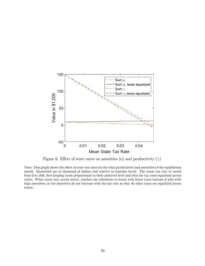

for some f 0 isin F hence there exists at least one w isin micro(f 0) for whom
tmicro(w)w gt 0 (B7)
But (B7) contradicts (B6) In the second case we have
0 gt ξτ (tmicro(w0)w0 ) (B8)
for some w0 isin W If we take f = micro(w0) then (B8) and (B6) together imply that X 0 gt tmicro(w)w = tfmicro(f)
wisinmicro(f)
contradicting (B5)
For τ lt 1 ξτ (middot) is strictly increasing and the conclusion of the proposition follows from the following more general result
Proposition 2rsquo Suppose that ξ(middot) is strictly increasing that [micro t] is stable under ξ(middot) and that [micro t] is stable under ξ(middot) with ξ(middot) le ξ(middot) Then [micro t] (under ξ(middot)) cannot Pareto dominate [micro t] (under ξ(middot))38
Proof Pareto dominance of [micro t] (under ξ(middot)) over [micro t] (under ξ(middot)) would imply that
γfmicro(f ) minus tfmicro(f) ge γfmicro(f ) minus tfmicro(f ) (B9)
+ ξ(ˇ + ξ(ˆαmicro(w)w tmicro(w)w) ge αmicro(w)w tmicro(w)w) (B10)
with strict inequality for some f or w However stability of [micro t] under ξ(middot) implies that
γfmicro(f ) minus tfmicro(f) ge γfmicro(f ) minus tfmicro(f ) (B11)
αmicro(w)w + ξ(tmicro(w)w) ge αmicro(w)w + ξ(tmicro(w)w) ge αmicro(w)w + ξ(tmicro(w)w) (B12)
where the second inequality in (B12) follows from the fact that ξ(middot) ge ξ(middot) Combining (B9) and (B11) gives
tfmicro(f) ge tfmicro(f) (B13)
38We say that an arrangement [micro t] (under ξ(middot)) Pareto dominates arrangement [micro t] under (under ξ(middot)) if
γfmicro(f) minus tfmicro(f) ge γfmicro(f) minus tfmicro(f ) forallf isin F
αmicro(w)w + ξ(tmicro(w)w) ge αmicro(w)w + ξ(tmicro(w)w) forallw isin W
with strict inequality for some i isin F cup W
44
for each f isin F while combining (B10) and (B12) gives
ξ(tmicro(w)w) ge ξ(tmicro(w)w)
tmicro(w)w ge tmicro(w)w (B14)
for each w isin W where the second line of (B14) follows from the fact that ξ(middot) is strictly increasing Strict inequality must hold in (B13) or (B14) for some f or w In the first of these cases we have
tf 0 micro(f 0) gt tf 0 ˇ micro(f 0)
for some f 0 isin F hence there exists at least one w isin micro(f 0) for whom
ˆ gt ˇtmicro(w)w tmicro(w)w (B15)
But (B15) contradicts (B14) In the second case we have
tmicro(w0)w0 gt tmicro(w0)w0 (B16)
for some w0 isin W If we take f = micro(w0) then (B16) and (B14) together imply that X X ˇ ˆtmicro(w)w gt tmicro(w)w
wisinmicro(f) wisinmicro(f )
hence we find that
tfmicro(f) gt tfmicro(f )
contradicting (B13)
B4 Proof of Theorem 1
If micro = micro then the theorem is trivially true Thus we consider a wage market in which [micro t] is stable under tax τ [micro t] is stable under tax τ τ gt τ and micro 6= micro The stability conditions for the firms imply that
γfmicro(f ) minus tfmicro(f) ge γfmicro(f ) minus tfmicro(f ) (B17)
γfmicro(f ) minus tfmicro(f) ge γfmicro(f ) minus tfmicro(f ) (B18)
these inequalities together imply that X X tfmicro(f ) minus tfmicro(f) ge tfmicro(f) minus tfmicro(f) (B19)
f isinF fisinF
45
As the market is a wage market we have
ξτ (tmicro(w)w) = (1 minus τ)tmicro(w)w and ξτ (tmicro(w)w) = (1 minus τ)tmicro(w)w
hence the stability conditions for the workers imply that
αmicro(w)w + (1 minus τ)tmicro(w)w ge αmicro(w)w + (1 minus τ)tmicro(w)w (B20)
αmicro(w)w + (1 minus τ)tmicro(w)w ge αmicro(w)w + (1 minus τ)tmicro(w)w (B21)
Summing these inequalities and applying Lemma 1 we obtain X X (1 minus τ) tfmicro(w) minus tfmicro(f) ge (1 minus τ) tfmicro(f) minus tfmicro(f) (B22)
fisinF fisinF
Combining (B19) and (B22) we find that X X (1 minus τ) tfmicro(w) minus tfmicro(f) ge (1 minus τ) tfmicro(w) minus tfmicro(f) (B23)
fisinF fisinF
Since τ lt τ (B23) implies that X tfmicro(f) minus tfmicro(f) ge 0 (B24)
f isinF
Next using (B18) and (B21) we find that X X M(micro) minus M(micro) = (γfmicro(f) minus γfmicro(f )) + (αmicro(w)w minus αmicro(w)w)
f isinF wisinW X X ge tfmicro(f) minus tfmicro(f) minus (1 minus τ) tmicro(w)w minus tmicro(w)w
fisinF wisinW X = τ tfmicro(f ) minus tfmicro(f ) ge 0
f isinF
where the final inequality follows from (B24)
B5 Proof of Proposition 1
Assume a matching micro is stable under tax τ In a wage market if we re-normalize the workers utilities by dividing by (1 minus τ) then a match that is stable with the renormalized utilities and no taxation is also stable with the original utilities and tax τ
αmicro(w)w + (1 minus τ)tmicro(w)w ge αfw + (1 minus τ)tfw
lArrrArr 1
αmicro(w)w + tmicro(w)w ge 1
αfw + tfw (B25)1 minus τ 1 minus τ
46
Combining (B25) with the standard firm stability conditions
γfmicro(f) minus tfmicro(f) ge γfD minus tfD
gives a matching market with quasilinear utility It is known (eg Kelso and Crawford (1982) Hatfield et al (2013)) that in such markets only an efficient matching can stable So micro must maximize the total of the re-normalized match values X X 1
micro isin arg max γfmicro(f ) + αmicro(w)w micro (1 minus τ)
fisinF wisinW
For the second and third results define a function X W (λα λγ ) = max λααfmicro(f) + λγ γfmicro(f)
micro f isinF
which is convex in both λα and λγ because it is the maximixation of a linear function By the envelope theorem the derivatives of W are
partW (λα λγ ) X = γfmicro(f )
partλγ fisinF
partW (λα λγ ) X X = αfmicro(f ) = αwmicro(w)
partλα fisinF wisinW
which are the firmsrsquo and workersrsquo match values respectively It is sufficient to show that whenever they exist (a) partW (λα λγ ) partλγ is nondecreasing
in λγ and (b) partW (λα λγ ) partλα is nonincreasing in λγ The first point follows directly from the convexity of W To see that the cross-derivative is non-positive note that W is positive homogenous
of degree one so whenever the derivatives exist we get by Eulerrsquos homogenous function theorem that
partW (λα λγ ) partW (λα λγ )W (λα λγ ) = λα + λγ
partλα partλγ
Hence partW (λα λγ ) 1 partW (λα λγ )
= W (λα λγ ) minus λγ
partλα λα partλγ
λγ partW (1 λγ λα) = W (1 λγ λα) minus
λα partλγ
which means part partW (λα λγ ) 1 partW (1 λγ λα) 1 partW (1 λγ λα) λγ part2W (1 λγ λα)
= minus minus lt 0partλγ partλα λα partλγ λα partλγ λα2 part(λγ )2
again using the convexity of W Taking λα = 1 and λγ = 1 minus τ gives the proposition
47
B6 Derivation of Equation (A1)
Summing (B20) across women and (B17) across men we find that X X αmicro(w)w minus αmicro(w)w ge (1 minus τ) tmicro(w)w minus tmicro(w)w
wisinW wisinWX X tmicro(w)w minus tmicro(w)w ge γfmicro(f ) minus γfmicro(f)
fisinF f isinF
Since Proposition 1 tells us that X γfmicro(f) minus γfmicro(f ) ge 0
fisinF
we can combine (B26) and (B27) to get P αmicro(w)w minus αmicro(w)wPwisinW ge (1 minus τ) γfmicro(f) minus γfmicro(f)fisinF
so that we find P P f isinF γfmicro(f) minus γfmicro(f ) wisinW αmicro(w)w minus αmicro(w)w
τ ge P + P f isinF γfmicro(f) minus γfmicro(f ) γfmicro(f) minus γfmicro(f) M(micro) minus M(micro)
f isinF
= P fisinF γfmicro(f ) minus γfmicro(f)
B7 Proofs of Proposition 4 and Corollary 1
Suppose that in a wage market both [micro t] and [micro t] are stable under tax τ conditions for the firms imply that
γfmicro(f ) minus tfmicro(f) ge γfmicro(f ) minus tfmicro(f )
γfmicro(f ) minus tfmicro(f) le γfmicro(f ) minus tfmicro(f )
so that
tfmicro(f ) minus tfmicro(f) ge tfmicro(f) minus tfmicro(f)
Meanwhile the stability conditions for the workers imply that
αmicro(w)w + (1 minus τ )tmicro(w)w ge αmicro(w)w + (1 minus τ)tmicro(w)w
αmicro(w)w + (1 minus τ )tmicro(w)w le αmicro(w)f + (1 minus τ)tmicro(w)w
so that
(1 minus τ)(tmicro(w)w minus tmicro(w)w) le (1 minus τ)(tmicro(f )w minus tmicro(f )w)
(B26)
(B27)
(B28)
The stability
(B29)
(B30)
(B31)
(B32)
(B33)
(B34)
48
Summing (B31) and (B34) across agents and using Lemma 1 we find that X X tfmicro(f) minus tfmicro(f) = tfmicro(f) minus tfmicro(f) (B35)
fisinF f isinF
For this equality to hold we must have equality in (B31) for each f isin F implying equality in (B29) and (B30) for each f isin F Similarly (B35) requires that (B34) hold with equality for each w isin W which implies equality in (B32) and (B33) for each w isin W Combining these equalities and summing across workers w isin W shows that X X
αmicro(w)w minus αmicro(w)w = (1 minus τ) tfmicro(f) minus tfmicro(f) wisinW f isinF X
= (1 minus τ) γfmicro(f ) minus γfmicro(f ) (B36) f isinF
If the firms are not indifferent in aggregate between micro and micro so that X γfmicro(f ) minus γfˇ 6 (B37)micro(f ) = 0
fisinF
we have P wisinW αmicro(w)w minus αmicro(w)w
τ = 1 + P (B38)γfmicro(f) minus γfmicro(f)fisinF
thereby showing Proposition 4 To see Corollary 1 observe that (B38) pins down a unique tax rate in the case that
(B37) holds Thus if there are two tax rates under which matchings micro and micro are both stable then we must have X
γfmicro(f ) minus γfmicro(f ) = 0 (B39) fisinF
But then we also have X αmicro(w)w minus αmicro(w)w = 0 (B40)
wisinW
by (B36) Together (B39) and (B40) imply M(micro) minus M(micro) = 0 as desired
C Simulations of non-wage markets
We run 500 simulations of a one-to-one market with twenty agents on each side of the market and match values independently and identically distributed according to a uniform distribution on [minus5 5] We vary the tax rate τ from 0 to 99 in increments of 01 For each tax rate we find the manager-optimal stable arrangement and calculate the total match value ndash if there are multiple stable arrangements the manager-optimal arrangement is the one preferred by all managers Non-monotonicities in the total match value of stable matchings
49
appear in over half of the markets (55) There may be additional non-monotonicities that we do not observe because we cannot vary τ continuously However the non-monotonicities we fail to observe necessarily occur over very small ranges of τ as we observe all non-monotonicities that persist over values of τ for a range of 01 or more
Table 3 Summary of the non-monotonicities arising in simulated markets
Range of τ [0 25) [25 5) [5 75) [75 1) All τ
Fraction of markets with non-monotonicity
0006 0088 0190 0394 0548
Avg size of non-monotonicity as fraction of range
0021 0066 0111 0140 0120
Fraction of deadweight loss from taxation due to non-monotonicity
0076 0070 0051 0027 0037
Note The table summarizes 500 simulations of one-to-one matching markets with 20 agents on each side of the market All agentsrsquo match values are independently and identically distributed according to a uniform distribution on [minus5 5] We vary the tax rate τ from 0 to 99 in increments of 01 For each tax rate we find the manager-optimal stable arrangement and calculate the total match value Row 1 presents the fraction of markets that have non-monotonicities in a given tax rate range Row 2 presents the average size of non-monotonicities within each range normalized as a fraction of the (within-market) gap between the highest and lowest total stable match values calculated for any tax rate Row 3 presents the average fraction of taxation deadweight loss that is due to non-monotonicity across all markets The deadweight loss from non-monotonicity is computed for each tax rate τ as the difference between the highest total match value for a tax rate τ ge τ and the total match value under tax rate τ it is divided by the total deadweight loss from taxation at tax rate τ which is computed as the difference in total match value between the efficient matching and the matching stable under tax rate τ
Most markets have relatively small losses from non-monotonicity mostly occurring at high tax rates but some have dramatic non-monotonicities Table 3 summarizes the non-monotonocities arising in our simulations Row 1 shows the fraction of markets that have non-monotonicities in a given tax rate range While the majority of non-monotonicities occur at very high tax rates 10 of our simulation markets have non-monotonicities at tax rates below 50 Row 2 gives the (normalized) average size of the non-monotonicities in each tax rate range Again we see that non-monotonicities are most significant for high tax rates Row 3 incorporates information on the persistence of non-monotonicities by computing the fraction of the deadweight loss from taxation that is due to a non-monotonicity The fraction his is relatively high for lower tax rates because there is less total deadweight loss at those tax rates Overall our simulations suggest non-monotonicities in the tax rate are not just artifacts
of example selection However they also suggest that non-monotonicities are relatively rare at more realistic tax rates (τ isin [0 5)) and tend not to persist over large ranges of τ 39
39Increasing the sample size does not appear to decrease the frequency or importance of non-monotonicities
50
D Lump Sum Taxation
While not typically phrased in the exact language of taxation lump sum taxes are present throughout labor markets They might take the form of costs for hiring (eg employee health care costs) or for entering employment (eg licensing requirements) In the marriage market context lump sum taxes can take the form of marriage license fees or tax penalties for marriage
D1 Lump Sum Taxation of Transfers
We first consider a lump sum tax that is levied only on (nonzero) transfers between match partners40 Such a lump sum tax on transfers ` corresponds to the transfer function (
= 0ξlump tfw minus ` tfw 6
(tfw) equiv` tfw tfw = 0
shown in Figure 10 Under this tax structure the case ` = 0 corresponds to the stan-dard (Shapley and Shubik (1971)) model of matching with transfers and the case ` = infin corresponds to (Gale and Shapley (1962)) matching without transfers
tfw
0 (tfw) ξlump 2 (tfw)
ξlump 5 (tfw)
ξlump
lumpFigure 10 Transfer function ξ (middot)`
We say that an arrangement or matching is stable under lump sum tax ` if it is stable given transfer function ξlump(middot)` A lump sum tax on transfers has an extensive margin effect that makes being unmatched
more attractive relative to matching with a transfer In non-wage markets41 a lump sum tax on transfers can also encourage matchings in which transfers are unnecessary42 As our
40An alternative approach to lump sum taxation which we discuss in the next section imposes a flat fee on all matches
41Since it is difficult to observe transfers in non-wage markets such as marriage markets it is somewhat hard to imagine taxing them Nevertheless lump-sum taxes on transfers could correspond to instituting a lump sum tax on gifts between spouses and flat fees for matching could correspond to requiring marriage license fees
42Consider the case of balanced one-to-one matching markets In such markets lump sum taxes on
51
()
next example illustrates this second distortion can cause the total match value of stable matchings to be non-monotonic in the size of the lump sum tax
Example 3 (Non-monotonicity) Consider a one-to-one market with two firms F = f1 f2 two workers W = w1 w2 and match values as pictured in Figure 11a Worker w1 likes f1 ndash who has a strong preference for w2 ndash but w2 prefers f2 When transfers are not allowed (or when there is a high lump sum tax on transfers ` ge 18) the only stable matching is the matching micro1 in which micro1(f1) = w1 and micro1(f2) = w2 as shown in Figure 11b This matching yields total match value of M(micro1) = 22
(a) Match values (b) Matching without Transfers
(` = infin) (1 10) (1 10)
w1 f1 w1f1
(20minus1) (20minus1)
(10 1) (10 1) w2 f2 w2f2
(d) Matching with Lump Sum Tax (c) Matching with Perfect Transfers (` = 12) (` = 0) (minus1 0)(11 0) w1f1w1f1
t = minus10 (10 9)t = 10
(2 5)
(0 minus1)
t = 18 ξf (t) = 6
t = 10 ξf (t) = minus2
t = 2 ξf (t) = minus10 (1 10) w2f2w2f2 t = 9
Figure 11 Example 3 ndash Non-monotonicity under a lump sum tax on transfers
Note Utilities net of transfers are above the lines (firmrsquos workerrsquos) Possible supporting transfers (when applicable) are below the lines Solid lines indicate the stable matching
When the lump sum tax is lowered to ` = 12 only the matching micro2 is stable where micro2(f1) = w2 and w1 and f2 are unmatched this matching gives a total match value M(micro2) = 19 as shown in Figure 11d When ` = 12 the tax is low enough that f1 can convince w2 to match with him but not low enough for w1 to hold onto f1 when it has the option of matching with w2 (or f2 to hold onto w2) Lowering the lump sum tax from 20 to 12 decreases the total match value of the stable matching and decreases the number of agents matched
transfers promotes pairing (f w) in which the match value γfw + αfw is evenly distributed between the two partners (γfw asymp αfw) so that transfers are unnecessary
52
We use simulations to confirm that Example 3 is not an exceptional case In the same small markets described in Appendix C with utilities uniformly distribution on [minus5 5] we find that match value is non-monotonic in the lump sum tax in 61 of our simulated markets In a strictly positive wage market worker match values are strictly negative (instead of
just non-positive) In strictly positive wage markets all matchings require a transfer so a lump sum tax on transfers does not distort agentsrsquo preferences among match partners ndash for a given transfer vector if a worker prefers firm f1 to f2 without a tax then that worker also prefers f1 to f2 under a lump sum tax Thus in strictly positive wage markets the matching distortion of the lump sum tax is only on the extensive margin ndash the decision of whether to match ndash under a higher lump sum tax fewer agents find matching desirable This intuition that lump sum taxes work on the extensive margin is captured in the following lemma where we use (micro) to denote the number of workers matched in matching micro
Lemma 2 In strictly positive wage markets reduction in a lump sum tax on transfers (weakly) increases the number of workers matched in stable matchings That is if matching micro is stable under lump sum tax ` matching micro is stable under lump sum tax ` and ` lt ` then
(micro) ge (micro)
In non-wage markets the conclusion of Lemma 2 is not true in general because distortion among match partners can dominate the extensive margin effect as in Example 3 As lump sum taxes do not distort among match partners in strictly positive wage markets
they can only reduce the efficiency of stable matchings in such markets by reducing the number of workers matched This idea that the distortion must be on the extensive margin combined with Lemma 2 gives the following result
Theorem 2 In strictly positive wage markets a reduction in a lump sum tax on transfers (weakly) increases the total match value of stable matchings That is if micro is stable under lump sum tax ` ˆ ` and ˆ ` then micro is stable under lump sum tax ˆ ` lt ˇ
M(micro) ge M(micro)
Theorem 2 indicates that in strictly positive wage markets match value increases mono-tonically as lump sum taxation decreases In strictly positive wage markets we can also bound the total match value loss from a
given lump sum tax
Proposition 5 In a strictly positive wage market let micro be an efficient matching and let microbe stable under lump sum tax on transfers ` Then
0 le M(micro) minus M(micro) le ` middot ((micro) minus (micro))
The intuition for Proposition 5 is that since the workers unmatched under a lump sum tax of ` have negative surplus from matching under that lump sum tax their surplus from matching could not be more than ` So the change in total value is less than the change in the number of unmatched workers times a maximum surplus of ` per worker
53
Finally we can show that for a fixed limit on the number of workers matched in the presence of a lump sum tax stable matchings in strictly positive wage markets must generate the maximal match value possible
Proposition 6 In a strictly positive wage market a matching micro can be stable under a lump sum tax on transfers only if
micro isin arg max [M(micro)] micro (micro)le(micro)
Proposition 6 shows that a lump sum tax is an efficient way for a market designer to limit the number of matches (in strictly positive wage markets) the matchings stable under lump sum taxation have maximal value given the taxrsquos implied limit on the number of agents matched Analogously if a market designer wants to encourage matches a lump-sum subsidy will maximize total match value for a given (subsidy-induced) lower bound on the number of agents matched For example Proposition 6 suggests that if a government wants to use tuition subsidies to encourage people to go to school then uniform tuition subsidies are more efficient than subsidies proportional to the cost of tuition
D2 Lump Sum Taxation of Matches
Some fee structures tax all pairings rather than just those that include nonzero transfers Such flat fees for matching can also be interpreted in the language of taxation they corre-spond to the transfer function
ξfee ` (tfw) equiv tfw minus `
Figure 12 shows this transfer function for different levels of `
ξfee 0 (tfw) ξfee 2 (tfw)
ξfee 5 (tfw)
tfw
Figure 12 Transfer function ξfee(middot)`
Unlike lump sum taxes on transfers flat fees for matching never distort among match partners ndash even in non-wage markets Flat fees for matching only have extensive margin effects and thus markets with such fees are similar to strictly positive wage markets with lump sum taxes on transfers43 As shown below the conclusions of Lemma 2 Theorem 2
43Indeed in strictly positive wage markets lump sum taxation of transfers is equivalent to lump sum taxation of matchings because workers never match without receiving a strictly positive transfer
54
and Propositions 5 and 6 always hold in markets with flat fees for matching
D3 Proofs
Proof of Lemma 2
In a strictly positive wage market all matches are accompanied by a strictly positive transfer hence a lump sum tax on transfers is equivalent to a flat fee for matching Thus Lemma 2 follows from the following slightly more general result Here and hereafter we say that an arrangement or matching is stable under flat fee ` if
it is stable given transfer function ξfee(middot)`
Lemma 2rsquo Reduction of a flat fee for matching (weakly) increases the number of workers matched in stable matchings That is if matching micro is stable under flat fee ` matching micro is stable under flat fee ` and ˆ ` then ` lt ˇ
(micro) ge (micro)
where (micro) denotes the number of workers matched in matching micro
Proof As [micro t] is stable under flat fee ` we have
γfmicro(f) minus tfmicro(f) ge γfmicro(f) minus tfmicro(f)
+ ˇ ` middot 1ˇ =w ge αˆ + ˇ ` middot 1ˆ =wαmicro(w)w tmicro(w)w minus ˇ micro(w)6 micro(w)w tmicro(w)w minus ˇ micro(w)6
where 1micro(w)6 is an indicator function that equals 1 if w is matched in matching micro and=w
0 if w is unmatched in matching micro Summing these inequalities across agents and using Lemma 1 we find that X X
γfmicro(f) minus γfmicro(f) + αmicro(w)w minus αmicro(w)w + ` middot ((micro) minus (micro)) ge 0 (D1) f isinF wisinW
Similarly as [micro t] is stable under flat fee `
γfmicro(f ) minus tfmicro(f) ge γfmicro(f ) minus tfmicro(f )
+ micro(w)w ` middot 1ˆ =w ge αˇ + micro(w)w ` middot 1ˇ =wαmicro(w)w tˆ minus ˆ micro(w)6 micro(w)w tˇ minus ˆ micro(w)6
these inequalities yield X X γfmicro(f ) minus γfmicro(f) + αmicro(w)w minus αmicro(w)w + ` middot ((micro) minus (micro)) ge 0 (D2)
f isinF wisinW
upon summation Adding (D1) and (D2) shows that
(`minus `)((micro) minus (micro)) ge 0
Thus if ˇ ` we must have (ˆ micro) this proves the result ` gt ˆ micro) ge (ˇ
55
Proof of Theorem 2
As in the proof of Lemma 2 Theorem 2 follows from the following slightly more general result
Theorem 2rsquo A reduction in a flat fee for matching (weakly) increases the total match value of stable matchings That is if micro is stable under flat fee ` micro is stable under flat fee ` and ˆlt ` then
M(micro) ge M(micro)
Proof Using (D2) and Lemma 2rsquo we find that X X M(micro) minus M(micro) = γfmicro(f) minus γfmicro(f ) + αmicro(w)w minus αmicro(w)w ge ` middot ((micro) minus (micro)) ge 0
fisinF wisinW
this proves Theorem 2rsquo
Proof of Proposition 5
As in the proof of Lemma 2 Proposition 5 follows from the following slightly more general result
Proposition 5rsquo Let micro be an efficient matching and let micro be stable under flat fee ` Then
0 le M(micro) minus M(micro) le ` middot ((micro) minus (micro))
Proof The Proposition is immediate from (D1)
Proof of Proposition 6
As in the proof of Lemma 2 Proposition 6 follows from the following slightly more general result
Proposition 6rsquo A matching micro can be stable under a flat fee only if
micro isin arg max M(micro) micro (micro)le(micro)
Proof From (D1) we see that if [micro ˇ ` then for any matching ˆ 6 ˇt] is stable under flat fee ˇ micro = micro
M(micro) minus M(micro) + ` middot ((micro) minus (micro)) ge 0 (D3)
If fewer workers are matched in micro than in micro (ie (micro) ge (micro)) (D3) implies that
M(micro) minus M(micro) ge ` middot ((micro) minus (micro)) ge 0
so that micro must have higher total match value than micro
56
References
247Sports ldquo2013 football recruiting team rankingsrdquo 2013 Online accessed 29-July-2016 Arcidiacono Peter Andrew Beauchamp and Marjorie McElroy ldquoTerms of en-dearment An equilibrium model of sex and matchingrdquo 2011 NBER Working Paper No 16517
Becker Gary S ldquoA theory of marriage Part IIrdquo Journal of Political Economy 1974 82 11ndash26
Blundell Richard Alan Duncan and Costas Meghir ldquoEstimating labor supply re-sponses using tax reformsrdquo Econometrica 1998 66 827ndash861
Boadway R M Marchand and P Pestieau ldquoOptimal linear income taxation in models with occupational choicerdquo Journal of Public Economics 1991 46 (2) 133ndash162
Boone Jan and Lans Bovenberg ldquoOptimal labour taxation and searchrdquo Journal of Public Economics 2002 85 (1) 53ndash97
Chetty Raj ldquoIs the taxable income elasticity sufficient to calculate deadweight loss The implications of evasion and avoidancerdquo American Economic Journal Economic Policy 2009 pp 31ndash52
Chiappori Pierre-Andre Bernard Salanie and Yoram Weiss ldquoPartner choice in-vestment in children and the marital college premiumrdquo American Economic Review 2017 forthcoming
Choo Eugene and Aloysius Siow ldquoWho marries whom and whyrdquo Journal of Political Economy 2006 114 (1) 175ndash201
Crawford Vincent P and Elsie Marie Knoer ldquoJob matching with heterogeneous firms and workersrdquo Econometrica 1981 49 437ndash450
Dupuy Arnaud and Alfred Galichon ldquoPersonality traits and the marriage marketrdquo Journal of Political Economy 2014 122 (6) 1279ndash1319 and ldquoA note on the estimation of job amenities and labor productivityrdquo 2017 IZA working paper 10909
ESPN ldquoESPN football power index-2013rdquo 2013 Online accessed 29-July-2016 Feldstein Martin ldquoTax avoidance and the deadweight loss of the income taxrdquo The Review of Economics and Statistics 1999 81 (4) 674ndash680
Fok Dennis Richard Paap and Bram Van DijkFok ldquoA Rank-ordered Logit Model with Unobserved Heterogeneity in Ranking Capabilitiesrdquo Journal of Applied Economet-rics 2012 27 (5) 831ndash846
Gabaix Xavier and Augustin Landier ldquoWhy has ceo pay increased so muchrdquo Quar-terly Journal of Economics 2008 123 49ndash100
Gale David and Lloyd S Shapley ldquoCollege admissions and the stability of marriagerdquo American Mathematical Monthly 1962 69 9ndash15
Galichon Alfred and Bernard Salanie ldquoCupidrsquos invisible hand Social surplus and identification in matching modelsrdquo 2014 Mimeo Scott Kominers and Simon Weber ldquoCostly concessions An empirical framework for matching with imperfectly transferable utilityrdquo 2017 Mimeo
Gentry William M and R Glenn Hubbard ldquoThe effects of progressive income taxa-tion on job turnoverrdquo Journal of Public Economics 2004 88 (11) 2301ndash2322
57
Hatfield John William and Paul Milgrom ldquoMatching with contractsrdquo American Eco-nomic Review 2005 95 913ndash935 Scott Duke Kominers Alexandru Nichifor Michael Ostrovsky and Alexan-der Westkamp ldquoStability and competitive equilibrium in trading networksrdquo Journal of Political Economy 2013 121 966ndash1005
Holzner Christian and Andrey Launov ldquoDo employed workers search efficiently Im-plications for the income tax systemrdquo 2012 Mimeo
Kelso Alexander S and Vincent P Crawford ldquoJob matching coalition formation and gross substitutesrdquo Econometrica 1982 50 1483ndash1504
Koopmans Tjalling C and Martin Beckmann ldquoAssignment problems and the location of economic activitiesrdquo Econometrica 1957 25 (1) 53ndash76
Legros Patrick and Andrew F Newman ldquoBeauty is a beast frog is a prince Assor-tative matching with nontransferabilitiesrdquo Econometrica 2007 75 1073ndash1102
Lockwood Benjamin Charles Nathanson and E Glen Weyl ldquoTaxation and the allocation of talentrdquo 2013 Mimeo
Mas-Colell Andreu Michael D Whinston and Jerry R Green Microeconomic Theory Oxford University Press 1995
Meyer Bruce D ldquoLabor supply at the extensive and intensive margins The EITC welfare and hours workedrdquo American Economic Review 2002 92 (2) 373ndash379
Mortensen Dale and Christopher Pissarides ldquoTaxes subsidies and equilibrium labour market outcomesrdquo 2001 Mimeo
National Collegiate Athletics Association ldquoWinning percentagerdquo 2013 Online ac-cessed 29-July-2016
Office of Postsecondary Education 2013 Online accessed 29-July-2016 Parker Simon C ldquoDoes tax evasion affect occupational choicerdquo Oxford Bulletin of Economics and Statistics 2003 65 (3) 379ndash394
Powell David and Hui Shan ldquoIncome taxes compensating differentials and occupa-tional choice How taxes distort the wage-amenity decisionrdquo American Economic Journal Economic Policy 2012 4 (1) 224ndash247
Quinzii Martine ldquoCore and competitive equilibria with indivisibilitiesrdquo International Journal of Game Theory 1984 135 41ndash60
Roth Alvin E ldquoThe economics of matching Stability and incentivesrdquo Mathematics of Operations Research 1982 7 617ndash628
Rothschild Casey and Florian Scheuer ldquoRedistributive taxation in the Roy modelrdquo The Quarterly Journal of Economics 2012 pp 623ndash668
Saez Emmanuel ldquoOptimal income transfer programs intensive versus extensive labor supply responsesrdquo Quarterly Journal of Economics 2002 117 (3) 1039ndash1073 ldquoReported incomes and marginal tax rates 1960-2000 Evidence and policy implica-tionsrdquo in James Poterba ed Tax Policy and the Economy MIT Press 2004
Shapley Lloyd S and Martin Shubik ldquoThe assignment game I The corerdquo International Journal of Game Theory 1971 1 111ndash130
Sheshinski Eytan ldquoNote on income taxation and occupational choicerdquo 2003 CESifo Working Paper No 880
Tax Foundation ldquoFederal and state level tax information 2013rdquo 2013 Online accessed 17-November-2016
58
Tervio Marko ldquoThe difference that CEOs make An assignment model approachrdquo Amer-ican Economic Review 2008 98 642ndash668
USA Today ldquoCoaches salaries of the division I FBSrdquo 2013 Online accessed 29-July-2016 Wikipedia ldquoHead coaches past performance at start of 2013 seasonrdquo 2013 Online accessed 01-June-2015
59
- Introduction
- General Model
- Taxation and Mismatch
-
- Renormalizing Utilities
- Implications for Tax Analysis
-
- Econometric Framework
-
- Renormalization
- Maximum Likelihood
-
- Productivity
- Identification Without Wages
-
- Application
-
- Data
-
- Sources
- Summary
-
- Estimates of Job Amenities and Productivity
- Simulations
-
- Federal Top Tax Rate and State Taxes
- Thresholds and Inframarginal Rates
-
- Conclusion
- Additional Theoretical Results
-
- Taxes cannot cause Pareto improvements
- The Effect of Very Small Taxes
- Multiple matches stable at a given tax rate
- Nonlinear taxes
-
- Proofs for Section 2 and Appendix A
-
- Existence of Stable Arrangements amp Equivalence with the Core and Competitive Equilibria
- Total transfers
- Proof of Proposition 2
- Proof of Theorem 1
- Proof of Proposition 1
- Derivation of Equation (A1)
- Proofs of Proposition 4 and Corollary 1
-
- Simulations of non-wage markets
- Lump Sum Taxation
-
- Lump Sum Taxation of Transfers
- Lump Sum Taxation of Matches
- Proofs
-
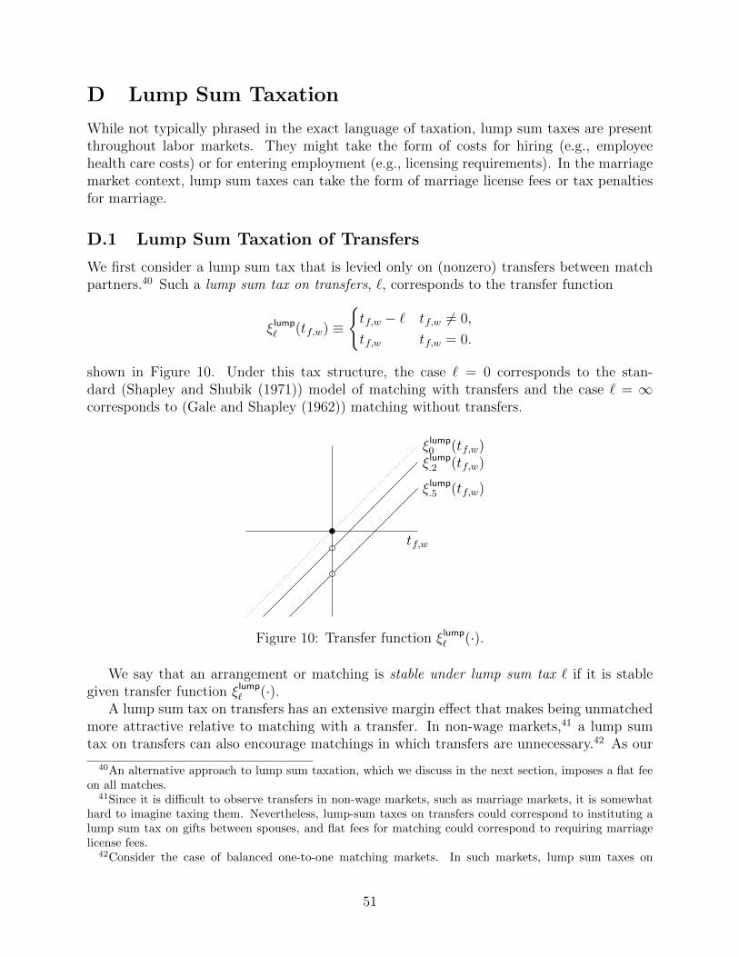
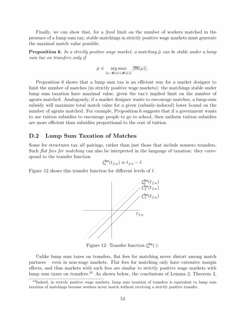