taxation and migration: evidence from major league baseball · taxation and migration: evidence...
TRANSCRIPT
Taxation and Migration: Evidence from Major League Baseball
Daniel GiraldoAdvisor: Jose Antonio Espın Sanchez
April 3, 2017
Abstract
Growing inequality in the developed world has led to calls for increasing countries’ top
marginal tax rates. Crucially, the optimal top marginal income tax rate depends on people’s
tendency to migrate in response to changes in the tax rate. Changes in tax rates and and
tax policy must take into account that increases in income tax rates may compel people to
leave a country or state. This paper studies how differences in the top marginal tax rates
affect the team and migrational choices of Major League Baseball players. Their elasticity of
migration with respect to the net of tax rate can be considered an upper bound for the same
elasticity in the entire labor supply, giving policy makers a worst-case scenario for migration
following a tax increase. I find that a 10% increase in the state and city’s top marginal tax
rate reduces a team’s wins in a season by about 2 (out of 162). If the elasticities estimated
represented the behavior of all of those in the top tax bracket, an increase of ten percentage
points in the average state’s top marginal tax rate would lead to a decrease of between 20
to 49 percent in the probability of a top income earner choosing to live in that state.
1

Daniel Giraldo 2
1 Introduction
Trends in inequality in developed nations have led to calls for increases in taxes on the
wealthy. Popular support for more redistributive policies and taxation of the wealthy came
to the fore in the wake of the Great Recession with the Occupy Wall Street movement. More
recently, Bernie Sanders, candidate for the Democratic Party’s 2016 presidential nomination,
centered his campaign on redistribution and ensuring that the wealthiest Americans pay their
“fair share” (Sanders, 2016). In the same spirit, Jeremy Corbyn, leader of the UK’s Labour
Party, has said he would raise taxes on the wealthy if elected Prime Minister (Wintour,
2015).
Some economists have added their voice to the growing chorus calling for higher taxes
on the wealthy. In his book, Capital in the Twenty-First Century, Piketty (2014) called for
a global wealth tax to combat increasing wealth inequality. With respect to income, Stiglitz
(2015) has called for a 5% increase in the top marginal tax rate to help combat inequality in
the United States. Piketty et al. (2014) argued that the optimal top marginal tax rate for
the United States is around 70 to 80 percent, almost twice its current level.
Arguments for increased tax rates on the wealthy need any behavioral response to the
increase in tax rates to not offset the increase in tax rates. Such a behavioral response could
come in the form of less hours worked or increased tax avoidance. Knowing the elasticity of
taxable income to the net of tax rate is crucial for assessing the effectiveness of an increase
in the top marginal tax rate. Since the tax cuts of the 1980s, a rich set of literature has
developed focused on estimating the elasticity of taxable income.1 There has also been
significant work in measuring capital mobility in response to changes international capital
tax rates.2 Not as much attention, however, has been focused on the migrational responses
to changes in labor income tax rates. In part, this is probably because it is much harder
for individuals to move than it is for capital and corporations. Increasing globalization and
1For review of this literature, see Saez et al. (2012).2see Griffith et al. (2010)

Daniel Giraldo 3
ease of migration, however, may make it easier for people, especially the wealthy, to move
in response to changes in tax rates.
In this paper, I study migrational responses to the net of tax rate using data on Major
League Baseball players between 1995 and 2014 as well as data on the teams, cities, and
states in which they are located. The quality of the individual level data on these players
provides sufficient controls to adequately estimate a response to changes in the tax rates. I
examine the effect of the top marginal tax rate on the salary of free agents and the ability
levels of free agents signed by a team. I also use multinomial logit to estimate baseball
players’ elasticity of migration with respect to the net of tax rate.
While I find no evidence to indicate that a change in the top marginal tax rate affects the
salary of free agents, I do find that an increase of 10 percentage points in the top marginal
tax rate of a team’s city and state of leads to a team signing players of lower quality, costing
the team about two wins per season in a season of 162 games. I also find evidence for a
migrational response with respect to a change in the net of tax rate and point estimates that
serve as upper bounds for the elasticity of migration with respect to the net of tax rate.
I proceed as follows. In Section 2, I examine the previous literature on migration and
taxation. Section 3 gives a brief overview of Major League Baseball. I specify the model for
player migration in Major League Baseball in Section 4. Section 5 describes the collection and
construction of the data. In Section 6, I explain the empirical methods and strategies used to
study the effects of the top marginal tax rate on team choice and player migration. Section
7 details the results. Finally, Section 8 concludes by discussing the policy implications.
2 Migration and Taxation: Previous Literature
The optimal tax is a decreasing function in the tendency to migrate in response to increases in
taxes (Mirrlees, 1982). Understanding people’s migrational responses to tax changes, then, is
important for setting tax rates. The previous work on the migrational effects of taxation has
left a few gaps and open questions. My study addresses three deficiencies in the literature.

Daniel Giraldo 4
First, it provides another angle with which to examine the issue of whether U.S. states
can redistribute and how responsive the wealthy are to changes in the tax rate. Second, it
explicitly looks at the tax rate induced migration of wealthy and high-skilled laborers across
many states over time; previous work has mostly focused on natural experiments in one or
two states at a time and has had a difficult time using quality data at the individual level.
Third, it provides an upper bound for the elasticity of migration to the net of tax rate within
the United States, given the high mobility of baseball players.
With regards to state migration, there has been conflicting evidence on the effect of
differences in state tax rates, though the more recent work has generally argued that there
is not much migrational response to an increase in state top marginal tax rates. Feldstein
and Wrobel (1998) echo Musgrave (1959) and Oates (1972) by arguing that, in the long
run, state and local taxes cannot redistribute income because freedom to migrate implies
that an increase in tax rates will lead to the out-migration of high income earners and an
in-migration of low income earners. These migrations will drive up wages in high tax states
and drive down wages in low tax states. For ease of reference, I will call this theory the
redistribution impossibility theory. Feldstein and Wrobel empirically support this theory by
regressing wage on the state’s net of tax share and finding a positive relationship between
the wage and the net of tax share. Young and Varner (2011) find this argument inadequate
because it does not show that migration is actually occurring, does not account for possible
reverse causation, and on some level simply demonstrates the definition of a progressive tax
system- wealthier people face higher tax rates.
Other studies of tax-induced migration within the United States have found weaker mi-
grational responses to tax changes. Leigh (2008) found that higher state taxes do have a
post-tax redistributive effect and that changes in state taxes did not affect migration flows.
Looking at multi-state Metropolitan Statistical Areas, Coomes and Hoyt (2008) find that
there is a statistically significant but economically modest out-migration from states with
higher taxes to states with lower taxes. Similarly, Bakija and Slemrod (2004) exploit differ-

Daniel Giraldo 5
ences in taxes faced by wealthy people in different states to find that states with higher taxes
have fewer federal estate tax returns filed. The effect is strongest for estate and inheritance
tax differences, but even these effects are relatively small when compared to the change in
collected tax revenue.
Studies of other countries, too, have reached similar conclusions: migrational responses
to differences in taxation within countries are small, especially when compared to what the
redistribution impossibility theory would suggest. Day and Winer (2006) study Canadian
aggregate migration data from 1974 to 1996 and analyze how differences in regional policies
(including personal income taxes) affect inter-province migration. They find that variation
in these regional policies had little, if any, impact on migration. In Switzerland, Liebig et al.
(2006) find that differences in income taxes among Swiss cantons induce modest inter-canton
migration, and that this induced migration is not enough to offset increased canton revenues
from the taxes.
Young and Varner (2011) summarize the literature’s hypotheses as to why there are no
large migrational responses to changes in tax rates: commuting is costly, searching for and
changing jobs is costly, people have friends and family they do not want to move away from,
and higher taxes usually mean more public goods, which may counteract the migrational
push effects of higher taxes. But maybe the wealthy are more responsive to tax changes;
maybe the amount the wealthy lose from an increase in the top marginal tax rate is large
relative to the commuting and moving costs associated with migration. A slew of recent
work has focused on wealthy individuals’ migrational responses to changes in tax rates. Alm
and Wallace (2000) have argued that rich people are more responsive to tax changes than
average people; their particular study looked at differences in reporting rates. By contrast,
after exploiting the natural experiment induced by New Jersey’s increase of the top marginal
tax rate by 2.6 percentage points, Young and Varner (2011) conclude that the migrational
response of the wealthy to changes in income tax rates is small; very little migration occurred.
Outside the U.S., researchers have found a stronger migrational response by the wealthy

Daniel Giraldo 6
in response to changes in tax rates. Kleven et al. (2013) took one of the first steps in
analyzing international migration in response to differential income tax rates by examining
the professional football player market in Europe. They found that domestic players have a
modest response to a change in the net-of-tax-rate and foreign players have a much larger
elasticity with respect to the net of tax rate. Akcigit et al. (2016) found similar results for
“superstar” inventors.
Previous work on the effect of the states’ differences in top marginal income tax rates
on sports salaries and migration in the United States shows a significant if modest effect.
Alm et al. (2012) studied free agents in Major League Baseball and found that an increase
in the top marginal tax rate of 1 percent increased a free agent’s final salary by $21,000 to
$24,000. In a study that explicitly considered the migrational effects of income tax rates,
Kopkin (2011) found a behavioral response in basketball players to an increase in tax rates:
teams with higher state and municipality top marginal income taxes had a lower average
skill of signed free agents.
Looking only at players who actually finished a contract and reached free agency, however,
would overestimate the tendency of players to move in response to changes in the net of tax
rate. This is because an analysis that looks only at actual free agents excludes players who
chose to stay on their team by signing a contract extension before the end of their contract.
These players had a choice to make and chose to stay in the same team; their decision
should be factored into any study that attempts to measure the tendency of players to move
in response to changes in the tax rate. The multinomial regression that I use allows me
to include not only free agents in the analysis, but also players who meet the experience
requirements for free agent eligibility but are still under contract.
Focusing on the players of Major League Baseball presents several advantages for the
study of migrational responses to differences in tax rates. First, if anybody is going to
overcome the frictions that prevent people from moving in response to changes in tax rates,
it would probably be professional athletes. Players are used to moving teams, earn almost
Daniel Giraldo 7
all their income from labor, and will only earn large amounts of income for a short amount
of time. In this respect, Major League Baseball players are probably more mobile than the
football players studied in Kleven et al. (2013) because there are fewer language and cultural
barriers in moving states than there are in moving countries.
Second, the nature of the data allows one to track individuals over a long period of time
and control for quality, personal characteristics, and other factors. Issues stemming from
lack of access to individual level data to track migration and control for different factors
have plagued previous studies. Third, baseball players, particularly the top players that
command high salaries, serve as a testing ground for what Young and Varner refer to as
“permanent millionaires” (Young and Varner, 2011). They hypothesize that one of the
reasons the increase in the New Jersey top marginal tax rate led to very little migration out
of the state is that most people are “transitory millionaires,” meaning that very few people
actually face the top marginal tax rate year after year. Because they do not face the top
marginal tax rate most of the time, a large portion of millionaires in any given year have
little reason to move out of a state in response to an increase in the top marginal tax rate.
In contrast, “permanent millionaires” may have a reason to move since they will face the top
marginal rate year after year. I argue, in Section 5, that baseball players can be considered
“permanent millionaires.” This paper serves as a beginning step towards understanding the
behavior of so-called permanent millionaires.
3 Major League Baseball, Economics, and Taxation
In this section, I give a brief overview of Major League Baseball (MLB) and touch on relevant
economic and taxation issues in the league. There are 30 teams in Major League Baseball.
One team is located in Canada, and the rest are in the United States. They are located
in 18 U.S. states, the District of Columbia, and Ontario. Each team has a 25-man roster,
which includes the players that are eligible to play in any given game. The 25 players can
be changed day-to-day and are picked from the 40-man roster, which includes everyone on

Daniel Giraldo 8
the team with a Major League Baseball contract.
A given season occurs entirely within a calendar year. The MLB season starts in March
with what is known as Spring Training. Teams take this time to prepare for the regular
season, and they usually spend this time in either Arizona or Florida. The regular season
consists of 162 games and starts in late March and early April. It runs through late September
or early October, depending on the year. The postseason takes place mostly in October and
ends in early November.
MLB has two leagues: the American League and the National League. Each league is
split into three divisions and each division has five teams.3 To qualify for the playoffs, a
team must either win their division or obtain one of two “wild-card” spots available to the
two best non-division winners in each league. Teams mostly play against teams in their own
league and division. Teams play 19 games against each opponent in their division and 20
games against teams in the opposite league. The rest of a team’s games are against non-
division opponents in the same league (Newman, 2012). While the two leagues have slight
rule differences in how the game is played, they observe the same rules when it comes to free
agency and contract bargaining.
Major League Baseball has experienced two waves of expansion since 1985. In 1993,
the league added the Florida Marlins and the Colorado Rockies. In 1998, the Arizona
Diamondbacks and the Tampa Bay Devil Rays (now just the Tampa Bay Rays) joined the
league to bring the total number of teams up to 30. Teams have moved very little since
these expansions. Only one team has moved states: in 2005, the Montreal Expos moved
to Washington D.C. and became the Washington Nationals. In 2012, the Florida Marlins
moved from Miami Gardens to a new stadium in downtown Miami and changed their name
to the Miami Marlins.
In addition to the 30 MLB teams, Major League Baseball largely controls what is known
as Minor League Baseball. Minor League Baseball consists of various leagues of descending
3This balance is a recent occurrence. Before 2013, the National League had 16 teams and the AmericanLeague had 14 teams. The Houston Astros agreed to move to the American League in 2013.
Daniel Giraldo 9
quality such as Triple-A, Double-A, and Class-A. Each Major League Baseball team is af-
filiated to a team in each of the leagues in Minor League Baseball. MLB teams use their
affiliated Minor League Baseball teams to develop young players. The players of each minor
league team generally have a contract with the team’s affiliated major league team.
MLB has a rich history of labor conflicts that has determined the current rules that
constrain player movement and contract negotiations. Before 1975, MLB contracts contained
what is known as the reserve clause. The clause stated that teams retained rights to a player
even after the player’s contract had expired. Players were not free to negotiate contracts
with other teams after their contract expired. After years of legal struggles and negotiations,
players finally obtained the right to free agency in 1975, although they had to have six years
of major league experience, could not re-enter the free agency pool for five years, and were
limited in the number of teams they could negotiate with (Pappas, 2002).
Currently, there are three mechanisms through which teams choose players and players
move teams: the draft, trades, and free agency. Every year, teams select high school and
college baseball players with no major league experience through the amateur draft. The
order of the draft is determined by how the teams performed in the previous season. A team
that drafts a player has exclusive negotiating rights with that player and the player cannot
sign or negotiate with any other team. Once a player has a contract with a team, that team
can choose to trade him to other teams in exchange for other players or money. Players have
very little recourse in preventing a trade, although many top players usually have a no-trade
clause in their contract that allows them to veto any trade they are a part of.
The final avenue for player movement is free agency. Although the exact rules of free
agency have changed with different collective bargaining agreements between the Major
League Baseball Player’s Association (MLBPA) and the team owners, the basic framework
of free agency has remained the same since 1985. Players who have at least six years of
major league experience are eligible for free agency.4 If a team loses a player to free agency,
4A player accumulates major league experience by being part of a major league team’s 40-man roster. Aplayer accumulates no major league experience when playing for a minor league team.

Daniel Giraldo 10
they are usually entitled to a compensatory draft pick. Players with less than six years of
service are not eligible for free agency but can ask for salary arbitration if they have more
than two years of experience.5
Two structures that constrain how much teams can spend on player salaries are the
competitive balance tax and the minimum salary. Since 1997, the MLB has had a competitive
balance tax. In its current form, there are certain thresholds to what teams may spend on
player salaries. If a team exceeds this threshold, then they are taxed by the league for a
portion of the amount for which they exceed the salary threshold (Cot’s, 2016). Since 1968,
the league has had a minimum salary. The current minimum salary for a player in a team’s
40-man roster is $507,500 (Cot’s, 2016).
One peculiar aspect of North American sports leagues is the jock tax. In the 1990s,
there were a wave of states and municipalities that began to enforce their income tax laws
on visiting athletes (Green, 1998). Though there have been multiple federal pushes for the
curbing of the practice, 15 of the 20 states and provinces with an MLB team currently
impose a jock tax (Hoffman and Hodge, 2004). States calculate the tax burden of non-
resident athletes using the duty days method. This method counts the total number of days
the athlete has spent inside the state and divides that number by the total number of “duty
days.” These include not only game days but also practice days, travel days, and preseason
activities (DiMascio, 2007). Different states apply different deductions based on taxes payed
in other localities, and I will take into account the details of the application of the jock tax
when calculating the top marginal tax rate players face in different teams.6
4 Model
In the following section, I present the model for player team choice. The model is based on
the migration models for football players and inventors presented in Kleven et al. (2013) and
5For a more detailed view of the history of collective bargaining agreements in MLB, see Cot’s (2016)6For a more detailed look at the intricacies of the jock tax see Hoffman and Hodge (2004)
Daniel Giraldo 11
Akcigit et al. (2016). There is a set J of teams, and there are n total teams in a particular
league. I index the teams so that each team j ∈ {1, 2, ..., n} = J . At time t, the players in
each team face tax rate τjt ∈ (0, 1). Each player p can earn wage ωjpt with team j. A player
receives utility from his after-tax income (1− τjt)ωjpt and utility µjpt ∈ R from non-income
factors that are player specific and team specific, such as market size or team ability. Let
u : R → R be an increasing function of a player’s after-tax income. Then player p’s utility
from playing on team j at year t is
Ujpt = u((1− τjt)ωjpt) + µjpt
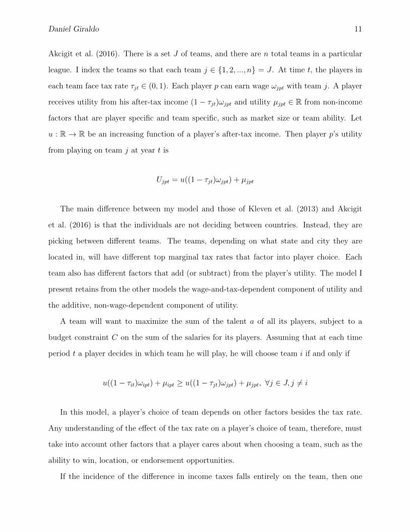
The main difference between my model and those of Kleven et al. (2013) and Akcigit
et al. (2016) is that the individuals are not deciding between countries. Instead, they are
picking between different teams. The teams, depending on what state and city they are
located in, will have different top marginal tax rates that factor into player choice. Each
team also has different factors that add (or subtract) from the player’s utility. The model I
present retains from the other models the wage-and-tax-dependent component of utility and
the additive, non-wage-dependent component of utility.
A team will want to maximize the sum of the talent a of all its players, subject to a
budget constraint C on the sum of the salaries for its players. Assuming that at each time
period t a player decides in which team he will play, he will choose team i if and only if
u((1− τit)ωipt) + µipt ≥ u((1− τjt)ωjpt) + µjpt, ∀j ∈ J, j 6= i
In this model, a player’s choice of team depends on other factors besides the tax rate.
Any understanding of the effect of the tax rate on a player’s choice of team, therefore, must
take into account other factors that a player cares about when choosing a team, such as the
ability to win, location, or endorsement opportunities.
If the incidence of the difference in income taxes falls entirely on the team, then one

Daniel Giraldo 12
would expect that teams in locations with higher income taxes have to pay players of a given
ability level more than teams in lower income tax states (Alm et al., 2012). On the other
hand, if the luxury tax or other payroll restrictions prevent teams from fully compensating
players for the income tax differential (Kopkin, 2011), or labor demand is rigid due to roster
constraints and skill complementarity (Kleven et al., 2013), then higher ability players will
tend to end up at teams with lower income taxes. I turn next to the issue of empirically
estimating players’ responsiveness to the tax rate.
5 Data
5.1 Baseball Statistics
The data gathered for this paper come from a diverse set of sources and are gathered for the
years 1995 to 2014. Most of the data on player statistics, including salary, have been retrieved
from the database maintained by Sean Lahman. Sean Lahman is a so-called “database
journalist” who has downloadable data on player statistics and salaries. Using his database, I
have been able to create datasets with batting, fielding, and pitching statistics for individual
players for each year. I gathered data on player WAR statistics using the site Baseball-
Reference.com. I am confident that both the Sean Lahman and Baseball-Reference data
are comprehensive; out of 37,402 player-year observations between 1985 and 2015, only 15
player-years in the Baseball Reference data did not have a match in the Lahman data and
only 1,352 player-years from the Lahman data did not have a match in the Baseball-Reference
data. The Lahman database also contains information on player salary. This data are much
less complete than the player performance data. Since 1995, there are 24,626 player-years
for which there are salary data. The number of player-year observations of players with
at least six years of service that have salary data since 1997 is 6,813. This translates to
about 378 observations per year and 12 observations per team per year. I collected team
winning percentages from Baseball-Reference. For some of the analyses run, I needed to

Daniel Giraldo 13
know which athletes were free agents each year. For this information, I turned again to
Baseball Reference, which has datasets of free agents for every year.
Above, I posited that baseball players can be considered “permanent millionaires.” I
examine the salary data collected to show that this is the case. Figure 1 shows the average,
median, 25th percentile, and minimum salary of free-agency eligible baseball players by year
for the data collected. The average salary has been above two million dollars each year since
1995. By 2009, the minimum salary of a baseball player was above $400,000. Since 1995,
the 25th percentile salary of free-agency eligible player has been greater than or equal to
$500,000 and by 1999 this figure had reached one million. Therefore, since 1999, at least
75% of free-agency-eligible baseball players’ annual salary has exceeded one million dollars.
Additionally, the median salary of free agency eligible baseball players has been above $1.5
million every year since 1995, meaning that at least 50% of free-agency-eligible baseball
players’ annual salary has exceeded one million dollars since 1995. These figures indicate
that baseball players are indeed permanent millionaires whose salary regularly gets taxed
at the top marginal tax rate. Studying their migrational responses to changes in the top
marginal tax rate serves as a first step towards understanding the migrational responses of
permanent millionaires to differences in the top marginal tax rate.
Looking at the salary summary statistics also allows me to validate the reliability of the
data collected by comparing the data’s summary statistics to official reports and estimates
done by others. On this front, the Sean Lahman data, though it does not contain salary data
for all players, appears to be representative of Major League Baseball salary. The minimum
salary in the Sean Lahman data tracks the minimum salary as dictated by the different
collective bargaining agreements agreed to since 1995. The average salary for all players by
year also follows closely the average salary as reported by the MLB Players Association. I
am therefore confident that the data collected is of good quality.

Daniel Giraldo 14
Figure 1: Selected Salary Summary Statistics for Free-Agency-Eligible Players
5.2 Tax Rate Data
I retrieved U.S. federal and state income tax data from the NBER’s Taxsim site (Feenberg
and Coutts, 1993). These tax rates take into account the different options taxpayers have in
different states to deduct state taxes from federal taxes or vice-versa. For Canada, province
and federal tax rates were obtained from the website of the Federal Revenue Agency. Some
Quebec tax data was gathered from Finances of the Nation (Treff and Perry, 2002). A few
of the cities and municipalities that have Major League Baseball teams in the United States
charge an additional income tax on residents and non-residents. I collected the data on city
and municipality tax rates by consulting the city websites and tax documents. For more
details on the sources for city and municipality tax data, see Appendix A.
As has been noted above, players do not simply face the tax rate from the state and
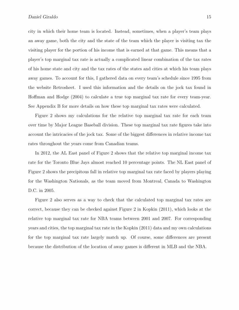
Daniel Giraldo 15
city in which their home team is located. Instead, sometimes, when a player’s team plays
an away game, both the city and the state of the team which the player is visiting tax the
visiting player for the portion of his income that is earned at that game. This means that a
player’s top marginal tax rate is actually a complicated linear combination of the tax rates
of his home state and city and the tax rates of the states and cities at which his team plays
away games. To account for this, I gathered data on every team’s schedule since 1995 from
the website Retrosheet. I used this information and the details on the jock tax found in
Hoffman and Hodge (2004) to calculate a true top marginal tax rate for every team-year.
See Appendix B for more details on how these top marginal tax rates were calculated.
Figure 2 shows my calculations for the relative top marginal tax rate for each team
over time by Major League Baseball division. These top marginal tax rate figures take into
account the intricacies of the jock tax. Some of the biggest differences in relative income tax
rates throughout the years come from Canadian teams.
In 2012, the AL East panel of Figure 2 shows that the relative top marginal income tax
rate for the Toronto Blue Jays almost reached 10 percentage points. The NL East panel of
Figure 2 shows the precipitous fall in relative top marginal tax rate faced by players playing
for the Washington Nationals, as the team moved from Montreal, Canada to Washington
D.C. in 2005.
Figure 2 also serves as a way to check that the calculated top marginal tax rates are
correct, because they can be checked against Figure 2 in Kopkin (2011), which looks at the
relative top marginal tax rate for NBA teams between 2001 and 2007. For corresponding
years and cities, the top marginal tax rate in the Kopkin (2011) data and my own calculations
for the top marginal tax rate largely match up. Of course, some differences are present
because the distribution of the location of away games is different in MLB and the NBA.

Daniel Giraldo 16
Figure 2: Relative Top Marginal Tax Rates by Team from 1999 to 2014

Daniel Giraldo 17
5.3 Controls
In order to control for other factors, I collected data about the particular metropolitan area of
each team. For teams in the United States, I retrieved information about the population and
total employment of each team’s Metropolitan Statistical Area (MSA) from the Bureau of
Economic Analysis. I retrieved Canadian Census Metropolitan Statistical Area employment
and population data from the CANSIM database created by Statistics Canada. I was only
able to gather this data for the years after 2000.
5.4 Summary Statistics and Data Overview
Before turning to estimating the different models, I examine summary statistics of the data
to evaluate relationships between variables and ensure that the data fit expectations. Full
summary statistics for all the variables can be found in Appendix C. For all of these tables,
a given performance statistic will have either the suffix“-Y” or “-C.” A performance statistic
with the suffix “-Y” indicates that it was a player’s statistic in the previous year. Performance
statistics with the suffix “-C” refer to a player’s career totals and averages to that point in
his career. Tables 7 and 8 summarize all of the variables for nonpitchers and pitchers who
are eligible for free agency i.e. have more than five years of MLB experience. These players
were not all necessarily free agents because some may have had years remaining on their
contract. Each variable is summarized for all years available (1995-2014), as well as for
the years 1999-2014 (years during which no new expansion teams joined) and for the years
1995-2001. The years 1995-2001 correspond to the years before the imposition of strong
competitive balance luxury taxes.
Analogously, tables 9 and 10 in Appendix C summarize the variables for all free agent
nonpitchers and pitchers. The definition of free agent that I used excluded players whose
contract was up but had played in the minor leagues the previous year. I excluded those
players because, since the players had not spent the previous year MLB, they did not have
comparable previous year statistics that could be used as controls.

Daniel Giraldo 18
Figure 3: Income Tax and Free Agent Distribution
Figure 3 plots the distribution of the relative income tax of the teams that free agents
signed with, the distribution of the relative income tax among all teams, and a superimposi-
tion of the kernel densities of the two histograms. The latter provides preliminary evidence
for the effect of the relative marginal income tax rate on player migration and team choice. It
shows that free agents disproportionately sign with teams with the lowest relative marginal
income tax rate, though the phenomenon is not visually dramatic.
Tables 11 and 12, found in Appendix C, give another preliminary glance at the relation-
ship between the top marginal tax rate and free agency choices. These two tables summarize
the different available statistics by tax quartile for nonpitcher and pitcher free agents, re-
spectively. Average salaries for nonpitchers tend to increase as one moves from the highest
quartile of relative marginal income tax to the lowest quartile of relative marginal income

Daniel Giraldo 19
tax. Moreover, many of the average performance statistics for nonpitchers, such as slugging
percentage, on-base percentage, and runs batted in (RBI), do not vary much by tax quar-
tile; theoretically, low relative marginal income taxes attract high-skill players, so one would
expect the average of these performance statistics to decrease as one moved to higher quar-
tiles. Notably, teams in the top quartile tend to have much bigger Metropolitan Statistical
Area population size and employment. Controlling for these factors may be important, as
metropolitan areas with high populations and employment may bring greater opportunities
for lucrative endorsements, attracting players to those cities.
In contrast to nonpitchers, the average salary for pitchers tends to decrease as one moves
from high relative marginal income tax quartiles to low relative marginal income tax quar-
tiles. Additionally, it appears that the average of pitcher performance statistics tends to
improve as one moves to higher relative marginal income tax quartiles. Earned run average,
a measure of how many runs a pitcher allows, is lowest in the highest quartile, indicating that
high-skill pitchers tend to sign with teams with high marginal income tax rates. Similarly,
the average number of games won the previous year is highest in the highest quartile. Al-
though the results of this exploratory data analysis seem to contradict the expected trends,
this approach is far from rigorous.
6 Empirical Strategy
My goal is to estimate the effect of a change in tax rates on the migration and team choice
of a given player. I estimate this effect using three different methods. The first estimates the
effect of the top marginal tax rate on player salary and is similar to the empirical strategy
used in Alm et al. (2012) and Kopkin (2011). For players with more than six years of major
league experience, I will estimate the following equation for free agents
Sjpt = β0 + β1τjt + β2Xpt + µt + ηp + εjpt (1)

Daniel Giraldo 20
Sjpt refers to the salary of player p in team j at time t. I control for skill and player
statistics Xpt in the estimation. I also include individual fixed effects ηp and time fixed
effects µt. The error term is εjpt. I include individual fixed effects to capture unobserved
characteristics of each player that influence his salary. Time fixed effects help account for
changes in salary from unobserved U.S. and MLB economic trends.
The coefficient of interest is β1, the effect of a one percentage point increase in the top
marginal tax rate on a player’s salary. This will provide an indication as to how an increase
in marginal tax rate affects salaries, which provides preliminary evidence on the effects of
tax rates on team choice and migration. If β1 is positive, then teams with high tax rates
must offer more money to players to compensate for the higher tax rate. For the estimation,
I use the top marginal tax rate, because baseball players, especially free agents, earn far
above the threshold for the top bracket in the income tax schedule. The top marginal tax
rate will approximate their average tax rate relatively well.
The second equation I want to estimate looks at the effect of the top marginal tax rate
on the skill of players on a team. For free agents, I would estimate
Ajpt = δ0 + δ1τjt + β2Npt + φt + ψp + ξjpt (2)
where Ajpt is the skill level of player p at time t playing for team j. In this estimation,
I also control for player characteristics Npt, time fixed effects φt, and team fixed effects ψj.
Here, ξjpt is the error term. Team fixed effects control for unobserved team characteristics
that give teams differential abilities to sign high-quality free agents. The coefficient of interest
in equation 2 is δ1, which measures the effect of a one percentage point increase in the
marginal tax rate on the skill of a players signed by team j in year t. Following the logic
of Kopkin (2011) and Kleven et al. (2013), if changes in the marginal tax rate are not fully
compensated by additional salary and affect migration, then δ1 will be negative, as more
talented players choose to go to teams with lower marginal tax rates.
Daniel Giraldo 21
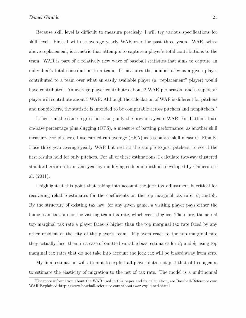
Because skill level is difficult to measure precisely, I will try various specifications for
skill level. First, I will use average yearly WAR over the past three years. WAR, wins-
above-replacement, is a metric that attempts to capture a player’s total contributions to the
team. WAR is part of a relatively new wave of baseball statistics that aims to capture an
individual’s total contribution to a team. It measures the number of wins a given player
contributed to a team over what an easily available player (a “replacement” player) would
have contributed. An average player contributes about 2 WAR per season, and a superstar
player will contribute about 5 WAR. Although the calculation of WAR is different for pitchers
and nonpitchers, the statistic is intended to be comparable across pitchers and nonpitchers.7
I then run the same regressions using only the previous year’s WAR. For batters, I use
on-base percentage plus slugging (OPS), a measure of batting performance, as another skill
measure. For pitchers, I use earned-run average (ERA) as a separate skill measure. Finally,
I use three-year average yearly WAR but restrict the sample to just pitchers, to see if the
first results hold for only pitchers. For all of these estimations, I calculate two-way clustered
standard error on team and year by modifying code and methods developed by Cameron et
al. (2011).
I highlight at this point that taking into account the jock tax adjustment is critical for
recovering reliable estimates for the coefficients on the top marginal tax rate, β1 and δ1.
By the structure of existing tax law, for any given game, a visiting player pays either the
home team tax rate or the visiting team tax rate, whichever is higher. Therefore, the actual
top marginal tax rate a player faces is higher than the top marginal tax rate faced by any
other resident of the city of the player’s team. If players react to the top marginal rate
they actually face, then, in a case of omitted variable bias, estimates for β1 and δ1 using top
marginal tax rates that do not take into account the jock tax will be biased away from zero.
My final estimation will attempt to exploit all player data, not just that of free agents,
to estimate the elasticity of migration to the net of tax rate. The model is a multinomial
7For more information about the WAR used in this paper and its calculation, see Baseball-Reference.comWAR Explained http://www.baseball-reference.com/about/war explained.shtml
Daniel Giraldo 22
discrete choice model. From the theoretical model, I have that, at year t with team j, a
player p has utility
Ujpt = u((1− τjt)ωjpt) + µjpt
Assuming that utility is a logarithmic function, and allowing for some possible factors beyond
the after-tax wage that may affect a player’s utility at a given team, the equation becomes
Ujpt = γ1log(1− τjt) + γ1log(ωjpt) + γ2Xpt + γj + νjpt (3)
where (1− τjt) is the net of tax rate. Xpt are player characteristics such as age, which may
affect a player’s decision to play in a given team, or a team’s willingness to hire him. Finally,
γj is a team fixed effect, and νjpt is the error term.
I fit McFadden’s choice model (McFadden, 1974), which takes into account the factors
that vary across teams in any given year as well as the changes for a given player’s charac-
teristics across years. This multinomial logit estimation allows me to take into account the
counterfactual top marginal tax rate the player would have faced had he chosen to play at
one of the other 29 teams. Adding controls to the estimation model allows me to take into
account other team characteristics that affect team choice as well.
The most important counterfactual comparison that cannot be made is that of salary. I
can only observe the actual salary of the player and not the salary that the player would have
earned had they chosen a different team. I attempt various specifications to try to make up
for this deficiency. In the first specification, I use only the net of tax rate, log(1 −MTR),
as the explanatory variable for team choice in the multinomial logit model. I expect this
estimation to yield an ambiguously signed or even negative coefficient on the net of tax
rate, because as the summary statistics show, wealthier teams tend to be located in places
with high top marginal tax rates. To control for this issue, I run a variety of specifications
that control for player abilities and characteristics, team fixed effects, and year-variant team
Daniel Giraldo 23
characteristics.
Let Pjpt = P(Ujpt > Uj′pt,∀ j′ ∈ J) be the probability that player p plays with team j
at time t. I assume that the error νjpt is type I extreme value distributed. Then, maximum
likelihood can estimate the multinomial logit. An estimation of γ1 allows me to estimate the
elasticity of the probability that player p plays with team j at time t with respect to the net
of tax rate (1 − τjt). In particular, if ε is this elasticity, then, following the calculations in
Kleven et al. (2013) and Akcigit et al. (2016), the elasticity for player p of the probability of
locating at team j on year t is
εjpt =d logPjpt
d log(1− τjt)= γ1(1− Pjpt).
By modifying calculations from the authors and by denoting I as the set of all players, I
can define team j level elasticities, εj, as the sum, weighted by Pjpt, of the elasticities for all
players for that team,
εj =γ1∑
i∈I(1− Pjpt)Pjpt∑i∈I Pjpt
I can then define the average elasticity of the probability of choosing a team to the net
of tax rate as the average weighted elasticities across the teams:
ε =30∑j=1
(γ∑i∈I(1− Pjpt)Pjpt∑30j=1
∑i∈I Pjpt
)
This ε is the parameter of interest, as it measures the migratory responsiveness of players
to changes in the net-of-tax rate. I calculate the average elasticity from the results of the
multinomial logit regression by modifying code from Kleven et al. (2013).

Daniel Giraldo 24
7 Results
7.1 Salary Effects
I first examine the effects of the top marginal tax rate on the salary paid to free agents
by estimating equation 1. I estimate the equation separately for pitchers and nonpitchers.
For both types of players, I include experience and experience squared in the equation, as
experience may be valuable for a team but in a nonlinear fashion; after a while, experience
signifies age, diminished performance, and a shorter playing horizon. Because one year’s
statistics may be a very different from a player’s overall career statistics, I include career
averages as well as previous year’s averages in estimating the salary equation.
Following Alm et al. (2012), I include both on-base plus slugging percentage and fielding
percentage as controls for nonpitchers. On-base plus slugging is a metric that quantifies
both a player’s ability to get on base and a player’s ability to hit well and run the bases. It
summarizes the offensive contributions of a player and so serves as a good metric for con-
trolling for player offensive ability. Fielding percentage measures the defensive effectiveness
of a player and so serves to control for player defensive ability.
For pitchers, I use wins, win/loss average, innings pitched, earned-run average, saves, and
strikeout-walk ratio as controls for non pitchers. I include saves to account for the differences
in the salary equations for starting pitchers and relief pitchers, as done in Krautmann et al.
(2003). Wins and losses are a common metric used to measure the success of a pitcher’s
outing, so I include wins and win/loss average. However, wins are dependent on the pitcher’s
team’s offensive and defensive ability. For this reason, I also include earned-run average,
strikeout-walk ratio, and innings pitched; these statistics are are much less influenced by
team ability.
Tables 1 and 2 show the results of the estimation for nonpitchers and pitchers, respec-
tively. The standard errors displayed are robust standard errors. I first run the estimation
using all of the player data for free agents that I have from 1995 to 2014. As noted above, I

Daniel Giraldo 25
Table 1: Salary Regression for Nonpitcher Free Agents
FE 1995-2014 FE 1995-2001 RE 1995-2014 RE 1995-2001Salary (000s) Salary (000s) Salary (000s) Salary (000s)
MTR -14.81 -6.040 -16.24 -32.52(23.95) (24.52) (22.54) (23.17)
Experience 649.3 364.7 195.1 513.7***(414.6) (229.5) (168.1) (173.5)
Experience Squared -22.85*** -33.17*** -18.58** -34.49***(8.398) (8.330) (7.782) (8.094)
On-Base Plus Slugging-Y 3469.9*** 571.0 4603.6*** 1755.6***(875.5) (643.2) (823.5) (590.5)
On-Base Plus Slugging-C 35147.4*** 25440.2*** 23190.7*** 18068.5***(7041.9) (7256.0) (2025.0) (2853.8)
Fielding Percentage-Y 846.4 3736.3 4331.5 1815.7(4307.5) (3854.7) (3592.4) (3093.3)
Fielding Percentage-C -7222.8 -56639.5* 1554.5 -405.6(46102.0) (33325.6) (9635.7) (9735.4)
Observations 1286 429 1286 429Individuals 625 241 625 241R-squared Overall 0.141 0.318 0.399 0.393
Standard errors in parentheses
* p<0.10, ** p<0.05, *** p<0.01

Daniel Giraldo 26
exclude from the sample of free agents all players who had played the previous year in the
minor leagues, as they do not have a comparable set of previous year’s statistics. Column 1
of Table 1 shows the results for a fixed effect model, while column 3 shows the results for a
random effects model. The coefficient on the top marginal tax rate is negative but very far
from significant at the 10 percent level. It is -14.81 (23.95) for the fixed effects model and
-16.24 (22.54) for the random effects model. Most of the coefficients of the other variables
are of the expected magnitude for both models. There is a positive coefficient on experience,
the previous year’s on-base plus slugging, the career average of on-base plus slugging, and
the previous year’s fielding percentage. Surprisingly, the coefficient on the career fielding
percentage is very negative for the fixed effects model.
Because Major League Baseball instituted more stringent luxury tax penalties for teams
with high payrolls starting with the 2001 Collective Bargaining Agreement, perhaps teams
could no longer spend to compensate free agents for lost wages due to differences in income
taxes. I therefore restricted my analysis to the years 1995-2001 in Columns 2 and 4, which
use fixed effects and random effects, respectively. The magnitude of the coefficient on the
top marginal tax rate decreases in the fixed effects model and increased in the random effects
model, though both coefficients remained negative and insignificantly different from zero at
the 10 percent level.
Table 2 shows the analogous results for pitchers. The specification shown in Column 1,
which is the fixed effects estimation that includes all free agents form 1995 to 2014, yields a
negative point estimate for the coefficient of MTR of higher magnitude than that for Column
1 for nonpitchers. However, when I restrict the sample to free agents form 1995 to 2001,
the coefficient becomes 42.20 (45.67), yet is still insignificant at the ten percent level. The
random effects results for all pitchers from 1995 to 2014 are in Column 3 and show a small
positive coefficient of 7.888 (30.46) on the top marginal tax rate. This coefficient shrinks
2.037 (39.14) when I restrict the sample to free agents from 1995 to 2001. Again, none of
the point estimates for the coefficient of interest are significant at the 10 percent level, or
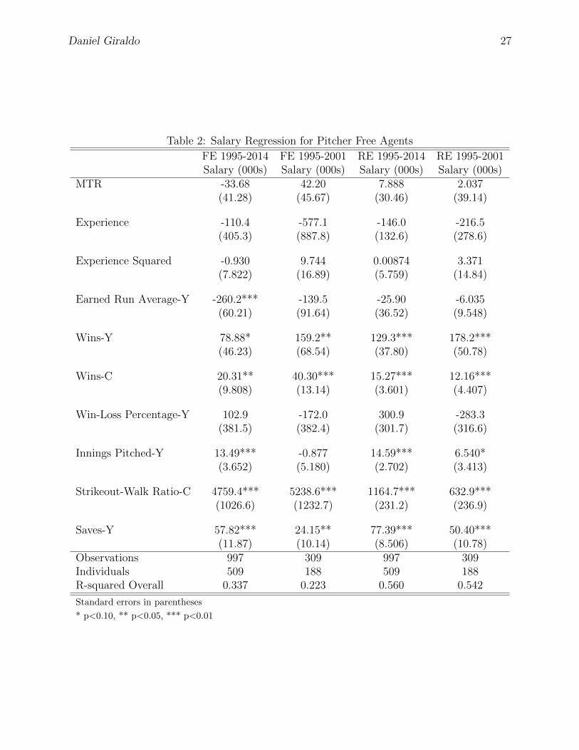
Daniel Giraldo 27
Table 2: Salary Regression for Pitcher Free Agents
FE 1995-2014 FE 1995-2001 RE 1995-2014 RE 1995-2001Salary (000s) Salary (000s) Salary (000s) Salary (000s)
MTR -33.68 42.20 7.888 2.037(41.28) (45.67) (30.46) (39.14)
Experience -110.4 -577.1 -146.0 -216.5(405.3) (887.8) (132.6) (278.6)
Experience Squared -0.930 9.744 0.00874 3.371(7.822) (16.89) (5.759) (14.84)
Earned Run Average-Y -260.2*** -139.5 -25.90 -6.035(60.21) (91.64) (36.52) (9.548)
Wins-Y 78.88* 159.2** 129.3*** 178.2***(46.23) (68.54) (37.80) (50.78)
Wins-C 20.31** 40.30*** 15.27*** 12.16***(9.808) (13.14) (3.601) (4.407)
Win-Loss Percentage-Y 102.9 -172.0 300.9 -283.3(381.5) (382.4) (301.7) (316.6)
Innings Pitched-Y 13.49*** -0.877 14.59*** 6.540*(3.652) (5.180) (2.702) (3.413)
Strikeout-Walk Ratio-C 4759.4*** 5238.6*** 1164.7*** 632.9***(1026.6) (1232.7) (231.2) (236.9)
Saves-Y 57.82*** 24.15** 77.39*** 50.40***(11.87) (10.14) (8.506) (10.78)
Observations 997 309 997 309Individuals 509 188 509 188R-squared Overall 0.337 0.223 0.560 0.542
Standard errors in parentheses
* p<0.10, ** p<0.05, *** p<0.01

Daniel Giraldo 28
even the 15 percent level.
The coefficients on performance metrics for pitchers are of the expected direction. As
wins, strikeout-walk ratio, innings pitched, and saves increase, there is an associated increase
in average in player salary. On the other hand, an increase in earned run average leads to
an associated decrease in average salary. The coefficients on experience are negative, which
falls in line with results seen in the literature, such as in Alm et al. (2012).
7.2 Average Ability of Free Agents
If teams in cities and states with higher income taxes do not compensate free agents for the
increased tax burden, then perhaps free agents respond to higher income taxes by migrating
or choosing to play for teams with lower top marginal income taxes. Since high-skilled
players can choose where to play more easily by virtue of their scarcity, this migration effect
would show up in that, all else held equal, teams in locations with higher top marginal
income taxes would sign less talented free agents. An estimation of equation 2 would yield
a negative coefficient on the top marginal tax rate.
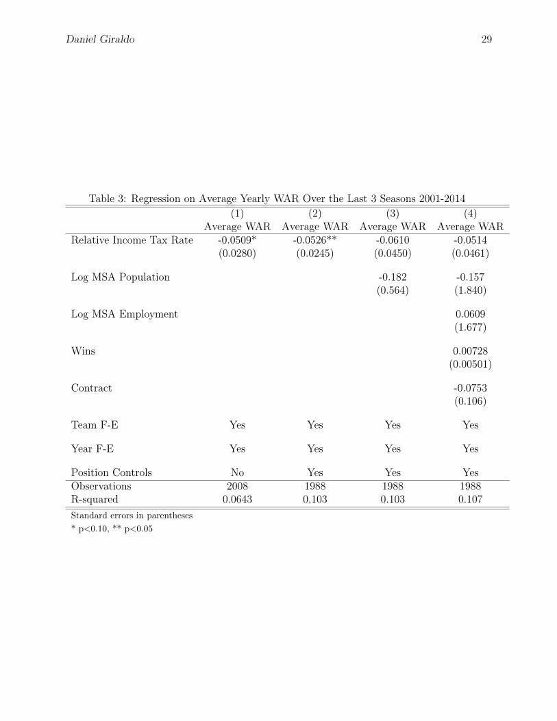
Table 3 displays the results of these estimations. The player-years included are from 2001
to 2014, as these are the years for which I have MSA controls. Column 1 regresses Average
WAR only on the relative income tax rate, team controls, and year controls. The resulting
coefficient of -0.05 is statistically significant at the 10% level. The coefficient becomes slightly
more negative, -0.053, when I introduce position controls in Column 2. It is also significant
at the 5 percent level.
Similarly, the coefficient moves little when I add at first just the logarithm of the
Metropolitan Statistical Area population in Column 3. All else held equal, a free agent
may prefer one team over another if the team has a larger market size and therefore more
opportunities for income through endorsements and other media avenues. Metropolitan Sta-
tistical Area log population can serve as a proxy for the team’s market size. In Column
4, I add log MSA employment, the number of games the team won the previous year, and
Daniel Giraldo 29
Table 3: Regression on Average Yearly WAR Over the Last 3 Seasons 2001-2014
(1) (2) (3) (4)Average WAR Average WAR Average WAR Average WAR
Relative Income Tax Rate -0.0509* -0.0526** -0.0610 -0.0514(0.0280) (0.0245) (0.0450) (0.0461)
Log MSA Population -0.182 -0.157(0.564) (1.840)
Log MSA Employment 0.0609(1.677)
Wins 0.00728(0.00501)
Contract -0.0753(0.106)
Team F-E Yes Yes Yes Yes
Year F-E Yes Yes Yes Yes
Position Controls No Yes Yes YesObservations 2008 1988 1988 1988R-squared 0.0643 0.103 0.103 0.107
Standard errors in parentheses
* p<0.10, ** p<0.05

Daniel Giraldo 30
whether the free agent chose to renew with the same team, but the coefficient moves little.
I add log MSA employment to include a different dimension of market size, as there will
probably be more opportunities for income in MSAs where there are more people earning a
labor income. I add the number of wins the team won the previous year to control for the
team’s quality, as a free agent may prefer, all else held equal, playing with a better team
rather than a worse team. Finally, I include the indicator for contract because a player may
be emotionally attached to his current team and be more inclined to sign with it, all else
held equal. Unfortunately, the addition of these controls in Column 3 and 4 increase the
standard error of the coefficient of relative income tax rate to the point where it is no longer
statistically significant at the 10% level.
As a robustness check, I run the above regressions using different measures for abilities.
The results can be seen in Appendix E. For all of the measures of ability, the coefficient on
the top marginal tax rate is negative, with varying levels of significance. The only exception
is when earned run average (a measure of pitcher performance) is used as the measure of
skill. However, the higher the earned run average, the worse the pitcher performance, so
the coefficient is also of the expected sign. When I used the average yearly WAR over the
past three years and restricted the sample only to pitchers, I once again obtained a negative
coefficient on the top marginal tax rate.
7.3 Multinomial Estimation
Finally, I turn to consider the estimation of the multinomial discrete choice model. I use
player-years between 1999 and 2014. In these years, no new expansion teams were formed.
In the first specification, I use only the net of tax rate as the explanatory variable. In the
second specification, I include team fixed effects and the interaction of team fixed effects
with individual player characteristics such as ability (WAR), experience, and experience
squared. These variables help control for unobserved characteristics in teams that affect
player choice, as well as for how the influence of these factors may vary with individual player

Daniel Giraldo 31
characteristics and ability. In the third specification, I use an alternate set of individual
player characteristics: WAR, age, age squared, and experience.
I control for an observed team characteristic that may affect player choice in the fourth
specification: the number of wins in the previous season. Finally, I control for another
observed team characteristic in the fifth specification, the logarithm of the Metropolitan
Statistical Area’s population. This could help control for factors such as city and market
size which may attract free agents because of endorsement or lifestyle considerations. In this
specification, I only use observations after the year 2001 because those are the ones for which
I have data on MSA population size.
Table 4: Multinomial Discrete Choice Estimations 1999-2014(1) (2) (3) (4) (5)
log(1-MTR) -0.413 1.554 1.841* 1.734* 0.748(0.433) (1.009) (1.024) (1.026) (1.327)
Wins 0.00239* 0.00230(0.00137) (0.00142)
Log MSA Population 0.281(0.330)
Team F-E No Yes Yes Yes Yes
Characteristics 1 x team F-E No Yes No No No
Characteristics 2 x team F-E No No Yes Yes YesElasticity -0.40 1.50 1.77 1.67 0.72
(0.418) (1.009) (1.024) (0.989) (1.28)Observations 214230 214020 214020 214020 201810Cases 7141 7134 7134 7134 6727
Standard errors in parentheses
* p<0.10, ** p<0.05
Table 4 shows the results for the multinomial logit estimation using data from 1999 to
2014 on players who are free agency eligible but not necessarily free agents. The reported
elasticities are only for the year 2014 as the elasticities are very similar across years and
Daniel Giraldo 32
computing for only one year greatly reduces computation time. As expected, the coefficient
of log(1−MTR) in column 1 is of ambiguous sign, as the standard error is of larger magnitude
than the point estimate.
Once I control for unobserved team characteristics and their interaction with player
characteristics in column 2, the coefficient of log(1 −MTR) becomes positive (1.554), as
expected, and its magnitude is larger than any of the estimates in Kleven et al. (2013),
suggesting that indeed MLB players can serve as an upper bound for the migrational elasticity
of the wealthy with respect to the net of tax rate. In column 2, the coefficient is still not
statistically significant at the 10 percent level and the implied elasticity is 1.50. In column 3, I
use different individual characteristics as controls and obtain a coefficient of higher magnitude
at 1.841, which is statistically significant at the 10 percent and implies an elasticity of 1.77.
The statistical significance of the coefficient remains once I control for team wins in the
previous year, while the coefficient falls to 0.748 once I control for the logarithm of MSA
population, loses statistical significance at the 10 percent level, and implies a much smaller
elasticity of 0.72.
The estimations in Table 4 assume that each player who is free agency eligible is making
a choice about where to play every year. That assumption is obviously not true, as players
have contracts that prevent them from moving in any given year. In Table 5, I restrict the
multinomial logit estimation to only consider free agent players. The estimations in this
case show a much higher coefficient for the net of tax rate than those in Table 4, giving an
even higher bound for the migrational elasticity of baseball players with respect to the net
of tax rate. Moreover, the coefficient for the net of tax rate is now statistically significant at
the 10 percent level for the second specification and is statistically significant significant at
the 5% level for the third and fourth specification. The coefficients for the second and fifth
specifications range from 2.171 to 2.979 and the elasticities range from 2.09 to 2.86.

Daniel Giraldo 33
Table 5: Free Agent Multinomial Discrete Choice Estimations 1999-2014
(1) (2) (3) (4) (5)
log(1-MTR) -0.168 2.344* 2.883** 2.979** 2.171(0.497) (1.310) (1.339) (1.345) (1.674)
Wins -0.00205 -0.00269(0.00213) (0.00221)
Log MSA Population 0.207(0.441)
Team F-E No Yes Yes Yes Yes
Characteristics 1 x team F-E No Yes No No No
Characteristics 2 x team F-E No No Yes Yes YesElasticity -0.16 2.26 2.77 2.86 2.09
(0.480) (1.260) (1.287) (1.293) (1.609)Observations 74340 73860 73860 73860 69960Cases 2478 2462 2462 2462 2332
Standard errors in parentheses
* p<0.10, ** p<0.05

Daniel Giraldo 34
8 Discussion and Policy Implications
In this paper, I have have estimated three different equations to analyze how the differences
in the top marginal tax rates in different states and cities affect the migratory and team
decisions of Major League Baseball players. First, I analyzed how the top marginal tax rate
affected the salary paid to free agents and found little to no effect. However, I did find that
an increase in the top marginal tax rate led to a decrease in the average ability of a team’s
free agent signees. Moreover, a multinomial logit estimation found that baseball players
show a large mobility response to changes in top marginal income tax rate.
Previously, Alm et al. (2012) had found that, for the years between 1995 and 2001, a
one percentage point increase in the top marginal tax rate was associated with an increase
in average free agent salary of $24,000. This result contrasts significantly with mine, since
I found a noisy, mostly negative, effect of top marginal tax rate on free agent salary. There
may be a couple of factors driving these difference is results. For years after 2001, perhaps the
imposition of more stringent luxury tax penalties prevented teams from fully compensating
free agents for differences in income tax rates. That is the hypothesis Kopkin (2011) puts
forth for why he estimates little to no effect of top marginal tax rate on the salary of basketball
free agents. The National Basketball Association has a salary cap and a luxury tax.
However, my results diverge from those of Alm et al. (2012) even for the years between
1995 and 2001. This seems especially strange because the group of players used to estimate
the equation seem to be very to similar their group of players, as shown by the summary
statistics. The results, however, are not directly comparable because we used different num-
bers of free agents. I used 429 nonpitcher observations between 1995 and 2001 (vs. 360) and
309 pitcher observations (vs. 267). I do not know which free agents they picked and how
specifically they picked them. I contacted the authors, but they unfortunately were not able
to assist me in finding out exactly which free agents they used.
In an attempt to replicate their results, I made two changes that may explain, though
Daniel Giraldo 35
not fully, the discrepancy. Tables 13 and 14 in Appendix D show the results of the modified
regressions. I made two modifications. The first was to exclude from the sample of free
agents all free agents who re-signed with their previous team. I did this because it is likely
that these players re-signed early in the free agency period and so may have been missed by
Alm et al. (2012). This modification brought the size of my sample of nonpitchers closer to
the size of Alm et al. (2012), as I had 297 observations. However, the size of pitcher sample
was still far from theirs (217 vs. 267).
The second change I made was motivated by an apparent error I noted in Alm et al.
(2012). They note that, in 2001, the top marginal tax rate in Toronto was 40.16% and
53.5% in Quebec. This is the top marginal rate one obtains if one makes two errors. First,
it doesn’t take into account the fact that Toronto charges an additional surtax on income
tax paid that would bring its 2001 top marginal tax rate to 46.41%. Second, the Quebec
top marginal tax rate assumes that Quebec faces the same federal income tax rate as the
rest of country. However, Quebec residents are taxed differently by the Canadian federal
government than the rest of the residents. As a result, the actual federal top tax rate in
Quebec in 2001 was not 29% but rather 24.2%, bringing the total top marginal tax rate in
Quebec in 2001 down to 48.72%
This combination of adjustments produce a coefficient of 26.47 on the top marginal tax
rate in the fixed effects model, suggesting that these changes help produce results closer to
Alm et al. (2012). However, the random effects model produces a negative coefficient, and
the results for pitchers are not closer to the results in Alm et al. (2012). See Appendix D
for more details.
The point estimates of the regressions from Table 3 suggest that free agents do respond
migrationally to the top marginal tax rate. An increase in the top marginal tax rate is
associated with a decrease in the average skill of the free agents a team signs. In particular,
a 10 percentage point increase in the top marginal tax rate is associated with a decrease
of 0.5 in the average WAR of free agents signed by a team. Considering that most starters

Daniel Giraldo 36
have a yearly WAR of around 2, the effect seems to be economically significant as well. For
example, in 2010 the difference in relative income tax rate between the Toronto Blue Jays
and the Texas Rangers was around 10%. Toronto signed around six free agents in 2010.
According to my estimates, Toronto’s relative top marginal income tax rate meant that,
had the Blue Jays been located in Texas, they would have, on average, been able to sign
players that would have added between two and three more wins in 2010 than the players
they actually signed. This finding mirror findings in other sports, such as those in Kopkin
(2011), who looked at free agent mobility in basketball.
The multinomial estimations retrieved elasticity estimates that ranged from 0.72 to 1.77
for all free-agency eligible players. These are larger than the range of 0.6 to 1.3 in Kleven
et al. (2013) for foreign football players and the range of 0.63 to 1.04 in Akcigit et al.
(2016) for foreign inventors. Although my data did not have the number of observations to
achieve the precision of these other studies, my point estimates suggest that indeed, baseball
players in the United States are a more mobile labor population between U.S. states than
are international football players and international investors between different countries.
My results when looking at free agents exclusively reveal, unsurprisingly, even higher
elasticities, which range from 2.09 and 2.86. These estimates are probably among the highest
that can be found for any group of laborers, as there are few laborers with the mobility
freedom of baseball free agents, who are freed of any contracts and previous commitment,
high-income earners, and psychologically prepared to move teams and cities. My estimates
for the mobility of baseball players can serve as an upper bound for the migrational response
to changes in income tax rates of the entire labor market. My results strengthen the finding
in Kleven et al. (2013) that “mobility could be an important constraint on tax progressivity”
(page 1923). They also provide a first glimpse into the migrational behavior of “permanent
millionaires” between U.S. states.
To put the elasticity numbers in perspective, suppose that all permanent millionaires in
the United States had the elasticity of migration probability with respect to the net of tax
Daniel Giraldo 37
rate that I have found in baseball players. Suppose that the average city saw its top marginal
tax rate decrease from 46 percent (the average top marginal tax rate in the sample) to 36
percent. Then the percentage increase in a permanent millionaire’s probability of choosing
to live in the average city would be
log(1− 0.46)− log(1− 0.36)
log(1− 0.46)× ε
where ε refers to the elasticity. Using the range of estimates produced by free agents would
suggest that the 10% decrease in top marginal tax rate would increase the probability that
millionaires would choose to live in that city by around 58% to 79%. If instead I used the
range of estimates produced by free agency eligible players, the probability would increase
by around 20% to 49%.
Ultimately, I do find evidence for strong tendencies by high-income individuals to move
states and cities in response to differences in top marginal income taxes. While the elasticities
suggest that baseball players and perhaps permanent millionaires are very migrationally
responsive to changes to the net of tax rate, because, as Young and Varner (2011) note, the
number of permanent millionaires is very small, the implications for tax policy are far from
clear. If the baseline probability that a permanent millionaire chooses to live in a city is small
to begin with, then the decrease in top marginal tax rate may not attract enough permanent
millionaires to a city or state to offset the decrease in tax revenues that come from reducing
the top marginal tax rate. A good course for future study would be to study these baseline
probabilities and calculate the number of permanent millionaires in each state.
Taken altogether, my results also suggest that it is not sufficient to simply look at how
wages and salaries respond in order to analyze the migrational effects of changes in the
top marginal tax rate. In industries with rigid and inelastic demand for high-skill laborers,
salaries may not be able to fully compensate for differences in tax rates between states.
Instead, firms may see a change in the composition of their laborers without seeing much

Daniel Giraldo 38
change in the salary of their laborers- high skill workers will tend to move towards the places
with lower tax rates. Therefore, looking only at salaries may lead one underestimate the
migrational effects of a change in top marginal tax rates and to miss the worker composition
effects that result from changes in tax rates.
I found no evidence to indicate that the salaries of baseball players adjust in response
to changes or differences in the top marginal tax rate; although states and cities have to
consider many more dimensions and people when weighing changes to tax policy, states
could increase top marginal tax rate and increase the tax revenue collected from baseball
players. The one caveat to increases in revenues comes from the jock tax. Because of the
jock tax, the true percentage collected from the top margin of the player’s salary by a state
will not increase one-to-one with the increase in top marginal tax rate. Since most states
credit players for tax paid to other states for visiting games, they will not be able to tax the
player’s salary earned in visiting games. On the other hand, the state also captures more tax
from visiting players, which may offset the losses from home players playing away games.
The results presented in this paper show that baseball players and the wealthy can display
significant migratory responses to changes in income tax rates. Governments at all levels
must take into account these responses when considering increasing top marginal tax rates.
Failure to take these responses could lead to lower tax revenue from loss of tax base or lower
economic productivity from the loss of skilled workers. The estimates made in this paper can
serve to calibrate policy or models to the worst-case scenario, because there is good reason
to believe that MLB baseball players can serve as an upper bound case for the elasticity of
migration with respect to the net of tax rate.
Acknowledgements
I would like thank my advisor, Professor Jose Antonio Espın Sanchez, for his guidance and
time. I would also like to thank Professor John Roemer and Professor Ebonya Washington for
their advice early on in the research process. I am also grateful to Sean Lahman, Retrosheet,

Daniel Giraldo 39
Baseball Reference, and the NBER for collecting and making publicly available some of the
data I used in this paper.

Daniel Giraldo 40
References
Akcigit, Ufuk, Salom Baslandze, and Stefanie Stantcheva, “Taxation and the In-ternational Mobility of Inventors,” American Economic Review, October 2016, 106 (10),2930–81.
Alm, James and Sally Wallace, “Are the Rich Different?,” in Joel Slemrod, ed., DoesAtlas Shrug?, Russell Sage Foundation at Harvard University Press, 2000, chapter 6,pp. 165–187.
, William H. Kaempfer, and Edward Batte Sennoga, “Baseball Salaries and IncomeTaxes: The Home Field Advantage of Income Taxes on Free Agent Salaries,” Journal ofSports Economics, 2012, 13 (6), 619–634.
Bakija, Jon and Joel Slemrod, “Do the Rich Flee from High State Taxes? Evidence fromFederal Estate Tax Returns,” Technical Report, National Bureau of Economic Research2004.
Cameron, A. Colin, Jonah B. Gelbach, and Douglas L. Miller, “Robust Inferencewith Multiway Clustering,” 2011, 29 (2), 238–249.
Coomes, Paul A. and William H. Hoyt, “Income Taxes and the Destination of Moversto Multistate MSAs,” Journal of Urban Economics, 2008, 63 (3), 920 – 937.
Cot’s Baseball Contracts, “CBA History,” 2016. https://www.baseballprospectus.com/compensation/cots/league-info/cba-history/
Day, Kathleen M. and Stanley L. Winer, “Policy-induced Internal Migration: AnEmpirical Investigation of the Canadian Case,” International Tax and Public Finance,2006, 13 (5), 535–564.
DiMascio, John, “The Jock Tax: Fair Play or Unsportsmanlike Conduct?” University ofPittsburgh Law Review, 2007, 68 (4).
Feenberg, Daniel and Elisabeth Coutts, “the TAXSIM Model,” Journal of Policy Anal-ysis and management, 1993, 12 (1), 189–194.
Feldstein, Martin and Marian Vaillant Wrobel, “Can State Taxes Redistribute In-come?,” Journal of Public Economics, 1998, 68 (3), 369–396.
Green, Richard E, “Taxing Profession of Major League Baseball: A Comparative Analysisof Nonresident Taxation, The,” Sports Law. J., 1998, 5, 273.
Griffith, Rachel, James Hines, and Peter Birch Srensen, “International Capital Tax-ation,” in Stuart Adam, Timothy Besley, Richard Blundell, Stephen Bond, Robert Chote,Malcolm Gammie, Paul Johnson, Gareth Myles, and James Poterba, eds., Dimension ofTax Design: The Mirrlees Review, Oxford: Oxford University Press, 2010, pp. 914–96.

Daniel Giraldo 41
Hoffman, David K. and Scott A. Hodge, “Nonresident State and Local Income Taxesin the United States: The Continuing Spread of “Jock Taxes”,” resreport 130, Tax Foun-dation July 2004.
Kleven, Henrik Jacobsen, Camille Landais, and Emmanuel Saez, “Taxation andInternational Migration of Superstars: Evidence from the European Football Market,”The American Economic Review, 2013, 103 (5), 1892–1924.
Kopkin, Nolan, “Tax Avoidance : How Income Tax Rates Affect the Labor MigrationDecisions of NBA Free Agents,” Journal of Sports Economics, 2011.
Krautmann, Anthony C., Elizabeth Gustafson, and Lawrence Hadley, “A Note onthe Structural Stablity of Salary Equations,” 2003, 4, 56–63.
Leigh, Andrew, “Do Redistributive State Taxes Reduce Inequality?,” National Tax Jour-nal, 2008, 61 (1), 81–104.
Liebig, Thomas, Patrick A. Puhani, and Alfonso Sousa-Poza, “Taxation And Inter-nal Migration - Evidence From The Swiss Census Using Community-Level Variation InIncome Tax Rates,” Hannover Economic Papers (HEP) dp-348, Leibniz Universitt Han-nover, Wirtschaftswissenschaftliche Fakultt October 2006.
McFadden, Daniel L., “Conditional Logit Analysis of Qualitative Choice Behavior,” inPaul Zarembka ed., Frontiers in Economics, Academic Press, 1974, chapter 4, pp. 105–142.
Mirrlees, J. A., “Migration and Optimal Income Taxes,” Journal of Public Economics,August 1982, 18 (3), 319–341.
Musgrave, Richard, The Theory of Public Finance, McGraw-Hill, 1959.
Newman, Mark, “MLB releases 2013 schedule with new wrinkles,” Online, MLB.com,2012, http://m.mlb.com/news/article/38287660/
Oates, Wallace E, Fiscal Federalism, Harcourt Brace Jovanovich, 1972.
Pappas, Doug, “A Contentious History: Baseball’s Labor Fights,” Online, ESPN.com,2002, http://static.espn.go.com/mlb/columns/bp/1427632.html
Piketty, Thomas, Capital in the Twenty-First Century, The Belknap Press of Harvarduniversity, 2014.
, Emmanuel Saez, and Stefanie Stantcheva, “Optimal Taxation of Top Labor In-comes: A Tale of Three Elasticities,” American Economic Journal: Economic Policy,February 2014, 6 (1), 230–71.
Saez, Emmanuel, Joel Slemrod, and Seth H. Giertz, “The Elasiticity of TaxableIncome with Respect to Marginal Tax Rates: A Critical Review,” Journal of EconomicLiterature, 2012, 50 (1), 3–50.

Daniel Giraldo 42
Sanders, Bernie, “The Transcript of Bernie Sanders Victory Speech,” The WashingtonPost 2016, https://www.washingtonpost.com/news/post-politics/wp/2016/02/10/the-transcript-of-bernie-sanderss-victory-speech/
Stiglitz, Joseph E., Rewriting the Rules of the American Economy, W.W. Norton & Com-pany, 2015.
Treff, Karin and David B. Perry, “Finances of the Nation,” resreport, Canadian TaxFoundation 2002.
Wintour, Patrick, “Jeremy Corbyn vows to raise taxes for therich if elected prime minister,” Online, The Guardian, 2015,https://www.theguardian.com/politics/2015/jul/22/jeremy-corbyn-vows-to-raise-taxes-for-the-rich-if-elected-prime-minister
Young, Cristobal and Charles Varner, “Millionaire Migration and State Taxation ofTop Incomes: Evidence from a Natural Experiment,” National Tax Journal, 2011, 64 (2),255–284.

43
Appendices
A Sources for the City Tax Rates
There are a total of nine cities that have a Major League Baseball team and levy an income
tax on residents and non-residents. For 2014, the cities had the following top marginal tax
rate for residents: Philadelphia 3.92%; New York City, 3.88%; Baltimore, 3.2%; Pittsburgh,
3%; Detroit, 2.4%; Cincinnati, 2.1 %; Cleveland 2%; Kansas City, 1%; and St. Louis 1%.
The data for top marginal tax rates in these cities between the years was collected from the
corresponding city websites, state tax documents, and city tax documents. Table 6 details
the exact sources used.8
Table 6: City Tax Rate Sources
City SourcePhiladelphia City of Philadelphia website8
New York City NYC Office of Management and Budget, “Tax Revenue Forecasting Doc-umentation: Financial Plan Fiscal Year 2015-2019,” 2015
Baltimore Individual income tax forms retrieved from the Comptroller of Marylandwebsite, taxes.marylandtaxes.com
Pittsburgh Pittsburgh Department of Finance website,pittsburghpa.gov/finance/earned-income-tax
Detroit Citizens Research Council of Michigan, “Detroit Government Revenues,”2013
Cincinnati City of Cincinnati website, http://cincinnati-oh.gov/finance/income-taxes/
Cleveland Division of Taxation, Department of Finance, City of Cleveland website,http://ccatax.ci.cleveland.oh.us/?p=effective
Kansas City Kansas City Star, “Kansas City voters overwhelmingly approve earningstax renewal,” April 5, 2016
St. Louis The PFM Group, “Earnings Tax Study City of St. Louis,” 2011, and theCity of St. Louis website
8The City of Philadelphia website used to contain a page listing wage taxes for residents and non-residentsdating back to 1995. I was able to access this page on January 7, 2017. The City of Philadelphia has sincerevamped its webpage, removing the page with wage tax data

44
B Constructing Marginal Tax Rates in Accordance with Jock Tax
A majority of the teams in Major League Baseball are located in states or cities that institute
a “jock tax.” Under the jock tax, athletes playing a game in a state that is not their home
state are required to pay a tax on the income they earned while playing the away game to
the state they are visiting. It is not a special tax levied only to athletes, but rather the
application of the state or city’s existing income tax to the visiting athlete. The states and
cities charge visiting athletes based on the number of games that they played at that state or
city and the total number of “duty days”. A duty day refers to a day in which an athlete is
required to go to work. For baseball players, this includes Spring Training games, practices,
home games and away games. For most teams, the number of duty days is around 207. To
determine the tax a visiting athlete owes, a state or city counts the number of games the
visiting athlete played there and divides this by the number by the number of duty days. The
jurisdiction then multiplies this fraction by the athlete’s total salary to get the total income
on which the jurisdiction will apply the tax. The only teams that were in jurisdictions that
did not charge a jock tax are the Toronto Blue Jays, the Montreal Expos, the Washington
Nationals, the Texas Rangers, the Florida Marlins, and the Seattle Mariners. Both cities
with income taxes and states with income taxes charge visiting athletes.
A hypothetical example may help clarify the way the jock tax works. Suppose player
A, who earns a salary of $20 million, plays for the Florida Marlins. Suppose that in 2014,
the Marlins played 6 away games against the Cincinnati Reds. The state of Ohio had
a top marginal rate on wages of 5.3% and the city of Cincinnati had an earnings tax of
2.1%. The player has spent 6207≈ 0.0299 of their duty days in Cincinnati. Cincinnati and
Ohio will levy their respective income tax on an income of 20, 000, 000 × 6207≈ $579, 710.
Cincinnati will end up charging $579, 710× 0.021 ≈ $12, 174 and Ohio will end up charging
$579, 710 × 0.053 ≈ $30, 725. In total, player A ends up paying about $42, 899 in taxes to
Ohio and Cincinnati for playing six games there.
45
One final wrinkle that enters the calculation of tax paid by a player is the possibility of
double taxation. Most states account for the possibility of double taxation and credit the
player for taxes paid to other states. That is, the home state, which would normally charge
an income tax based the player’s full salary, credits the player for the amount of tax they
have already paid, and charges the player the difference between the tax charged by the
visiting state and the full tax the home state would have charged if no visiting state had
levied the jock tax. The issue of double taxation also extends to cities that impose income
taxes. A player’s home city will not credit the player for taxes paid to outside states, but
will credit the player for taxes paid to outside cities.
Only Illinois engages in double taxation. If a player who plays for an Illinois plays an
away game at a jurisdiction that levies a jock tax, Illinois will not take into account the
amount of tax the player has already paid. Instead, Illinois will charge that player the full
tax the player would have had to pay had the game been a home game. Illinois is also the
only state that has in place a retaliatory jock tax. The state only levies a jock tax on players
who play for teams whose states also impose a jock tax. Visiting players from states like
Texas, Florida, or Washington, which do not have an income tax, do not get charged a jock
tax by Illinois.
To calculate the actual top marginal tax rate faced by each player in each team-year, I
downloaded full team schedules for each year from 1999 to 2014 from the website Retrosheet.
For each team-year, I calculated the number of away games they played at different locations,
and, using the duty days method, calculated the tax rate on the total salary that these away
games accounted for. I then added this to the home tax rate on the total salary for the
81 home games. I also added the tax rate that corresponds to the 45 spring training and
practice days, taking into account that Arizona and Michigan do not charge a state income
tax on spring training days. These tax rates, all added together, became the calculated top
marginal tax rate for each team-year.

46
C Summary Statistics
Below are different sets of summary statistics for the data I used.
Table 7: Summary Statistics for Nonpitchers Eligible for Free Agency
(1) (2) (3)
1995-2014 1995-2001 1999-2014
Salary (in thousands) 4694.4 (4759.8) 2922.2 (2677.9) 5272.0 (5047.1)
MTR 6.553 (2.355) 6.864 (2.349) 6.334 (2.227)
Relative Income Tax -0.00551 (2.174) -0.165 (1.881) 0.0389 (2.208)
MTR-Alternate 6.380 (2.216) 6.736 (2.451) 6.152 (2.044)
Experience 9.422 (2.906) 9.045 (2.384) 9.614 (3.064)
On-Base Percentage-Y 0.339 (0.0452) 0.346 (0.0475) 0.338 (0.0442)
On-Base Percentage-C 0.339 (0.0307) 0.337 (0.0317) 0.340 (0.0304)
Slugging Percentage-Y 0.429 (0.0882) 0.433 (0.0956) 0.429 (0.0865)
Slugging Percentage-C 0.429 (0.0624) 0.418 (0.0628) 0.434 (0.0620)
On-Base Plus Slugging-Y 0.768 (0.124) 0.779 (0.132) 0.767 (0.122)
On-Base Plus Slugging-C 0.768 (0.0861) 0.755 (0.0860) 0.774 (0.0858)
Batting Average-Y 0.268 (0.0374) 0.273 (0.0386) 0.268 (0.0367)
Batting Average-C 0.271 (0.0224) 0.269 (0.0228) 0.272 (0.0220)
Home Runs-Y 13.39 (11.40) 13.24 (12.15) 13.73 (11.36)
Home Runs-C 114.2 (102.3) 96.24 (86.79) 121.4 (106.6)
Runs Batted In-Y 54.50 (32.69) 54.53 (35.18) 55.41 (32.38)
Runs Batted In-C 474.0 (319.7) 423.4 (275.5) 495.3 (332.1)
Fielding Percentage-Y 0.982 (0.0218) 0.980 (0.0310) 0.983 (0.0146)
Fielding Percentage-C 0.981 (0.0111) 0.979 (0.0121) 0.981 (0.0107)
Observations 4124 1480 3294

47
Table 8: Summary Statistics for Pitchers Eligible for Free Agency
(1) (2) (3)
1995-2014 1995-2001 1999-2014
Salary (in thousands) 4355.0 (4183.3) 2728.3 (2397.6) 4813.5 (4402.7)
MTR 6.601 (2.346) 6.929 (2.358) 6.388 (2.196)
Relative Income Tax 0.0703 (2.139) -0.0652 (1.859) 0.0974 (2.151)
MTR-Alternate 6.388 (2.111) 6.748 (2.403) 6.172 (1.895)
Experience 9.219 (3.008) 8.801 (2.345) 9.358 (3.164)
Earned Run Average-Y 4.148 (2.413) 4.409 (3.622) 4.131 (2.580)
Earned Run Average-C 4.021 (0.634) 3.952 (0.636) 4.066 (0.634)
Wins-Y 6.733 (5.129) 6.967 (5.202) 6.730 (5.145)
Wins-C 60.74 (48.11) 59.99 (43.01) 60.76 (49.76)
Win-Loss Percentage-Y 0.508 (0.208) 0.514 (0.211) 0.508 (0.206)
Win-Loss Percentage-C 0.516 (0.0744) 0.516 (0.0705) 0.516 (0.0757)
Innings Pitched-Y 111.0 (67.41) 114.4 (68.13) 110.7 (67.32)
Innings Pitched-C 997.3 (691.2) 990.0 (639.8) 996.5 (709.5)
Strikeout-Walk Ratio-Y 2.428 (1.225) 2.209 (1.138) 2.464 (1.236)
Strikeout-Walk Ratio-C 2.156 (0.632) 2.040 (0.613) 2.178 (0.631)
Saves-Y 4.373 (10.47) 4.195 (9.954) 4.402 (10.60)
Saves-C 32.57 (72.03) 32.05 (68.08) 32.25 (72.32)
Observations 3056 1044 2511
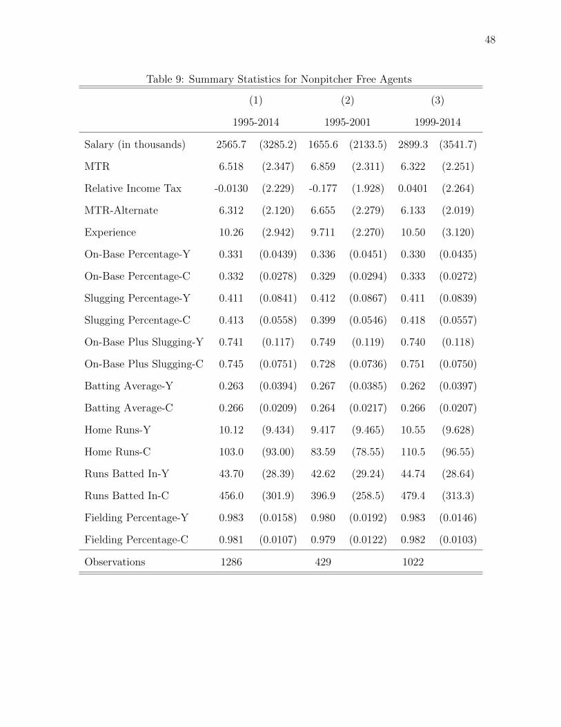
48
Table 9: Summary Statistics for Nonpitcher Free Agents
(1) (2) (3)
1995-2014 1995-2001 1999-2014
Salary (in thousands) 2565.7 (3285.2) 1655.6 (2133.5) 2899.3 (3541.7)
MTR 6.518 (2.347) 6.859 (2.311) 6.322 (2.251)
Relative Income Tax -0.0130 (2.229) -0.177 (1.928) 0.0401 (2.264)
MTR-Alternate 6.312 (2.120) 6.655 (2.279) 6.133 (2.019)
Experience 10.26 (2.942) 9.711 (2.270) 10.50 (3.120)
On-Base Percentage-Y 0.331 (0.0439) 0.336 (0.0451) 0.330 (0.0435)
On-Base Percentage-C 0.332 (0.0278) 0.329 (0.0294) 0.333 (0.0272)
Slugging Percentage-Y 0.411 (0.0841) 0.412 (0.0867) 0.411 (0.0839)
Slugging Percentage-C 0.413 (0.0558) 0.399 (0.0546) 0.418 (0.0557)
On-Base Plus Slugging-Y 0.741 (0.117) 0.749 (0.119) 0.740 (0.118)
On-Base Plus Slugging-C 0.745 (0.0751) 0.728 (0.0736) 0.751 (0.0750)
Batting Average-Y 0.263 (0.0394) 0.267 (0.0385) 0.262 (0.0397)
Batting Average-C 0.266 (0.0209) 0.264 (0.0217) 0.266 (0.0207)
Home Runs-Y 10.12 (9.434) 9.417 (9.465) 10.55 (9.628)
Home Runs-C 103.0 (93.00) 83.59 (78.55) 110.5 (96.55)
Runs Batted In-Y 43.70 (28.39) 42.62 (29.24) 44.74 (28.64)
Runs Batted In-C 456.0 (301.9) 396.9 (258.5) 479.4 (313.3)
Fielding Percentage-Y 0.983 (0.0158) 0.980 (0.0192) 0.983 (0.0146)
Fielding Percentage-C 0.981 (0.0107) 0.979 (0.0122) 0.982 (0.0103)
Observations 1286 429 1022

49
Table 10: Summary Statistics for Pitcher Free Agents
(1) (2) (3)
1995-2014 1995-2001 1999-2014
Salary (in thousands) 2949.4 (3096.7) 1977.6 (2061.6) 3236.3 (3285.0)
MTR 6.568 (2.308) 7.007 (2.499) 6.318 (2.108)
Relative Income Tax -0.0142 (2.082) -0.175 (1.866) 0.00890 (2.090)
MTR-Alternate 6.438 (2.093) 6.956 (2.575) 6.177 (1.787)
Experience 10.01 (3.144) 9.385 (2.168) 10.21 (3.319)
Earned Run Average-Y 4.341 (3.612) 4.879 (6.095) 4.323 (3.937)
Earned Run Average-C 4.076 (0.601) 3.959 (0.604) 4.137 (0.597)
Wins-Y 5.795 (4.504) 6.278 (4.565) 5.731 (4.493)
Wins-C 62.39 (48.53) 63.27 (40.73) 62.29 (50.74)
Win-Loss Percentage-Y 0.497 (0.211) 0.507 (0.203) 0.497 (0.211)
Win-Loss Percentage-C 0.504 (0.0686) 0.506 (0.0657) 0.504 (0.0705)
Innings Pitched-Y 100.1 (62.31) 107.0 (64.49) 99.20 (61.76)
Innings Pitched-C 1046.3 (696.9) 1071.5 (623.1) 1041.7 (720.6)
Strikeout-Walk Ratio-Y 2.234 (1.055) 2.035 (1.001) 2.247 (1.041)
Strikeout-Walk Ratio-C 2.070 (0.584) 1.984 (0.623) 2.069 (0.557)
Saves-Y 3.366 (8.842) 3.049 (8.041) 3.255 (8.716)
Saves-C 37.62 (78.46) 36.38 (75.22) 36.67 (77.61)
Observations 997 309 815

50
Table 11: Summary Statistics for Nonpitcher Free Agents by Tax Quartile 1999-2014
(1) (2) (3) (4)
Top 25% 25%-50% 50%-75% Lower 25%
Salary (in thousands) 2997.1 (3902.1) 2735.4 (3145.7) 3029.5 (3564.8) 3009.2 (3687.2)
MTR 8.897 (2.192) 6.527 (0.647) 5.562 (0.487) 3.685 (0.582)
Relative Income Tax 2.688 (2.152) 0.271 (0.509) -0.730 (0.313) -2.682 (0.462)
MTR-Alternate 8.242 (1.971) 6.527 (0.647) 5.562 (0.487) 3.685 (0.582)
Experience 10.90 (3.528) 10.45 (3.095) 10.08 (2.771) 10.66 (3.127)
On-Base Percentage-Y 0.331 (0.0496) 0.330 (0.0357) 0.328 (0.0407) 0.328 (0.0440)
On-Base Percentage-C 0.335 (0.0296) 0.333 (0.0243) 0.331 (0.0267) 0.333 (0.0260)
Slugging Percentage-Y 0.415 (0.0841) 0.406 (0.0799) 0.412 (0.0778) 0.410 (0.0907)
Slugging Percentage-C 0.423 (0.0572) 0.415 (0.0543) 0.416 (0.0545) 0.419 (0.0556)
On-Base Plus Slugging-Y 0.745 (0.124) 0.736 (0.107) 0.740 (0.107) 0.738 (0.127)
On-Base Plus Slugging-C 0.758 (0.0790) 0.749 (0.0716) 0.747 (0.0737) 0.752 (0.0737)
Batting Average-Y 0.262 (0.0449) 0.264 (0.0340) 0.261 (0.0347) 0.259 (0.0423)
Batting Average-C 0.268 (0.0209) 0.266 (0.0194) 0.265 (0.0207) 0.266 (0.0211)
Home Runs-Y 10.92 (9.789) 9.886 (8.912) 10.68 (9.304) 10.29 (9.668)
Home Runs-C 122.4 (107.0) 107.9 (99.17) 102.3 (85.76) 111.6 (94.01)
Runs Batted In-Y 45.81 (28.67) 43.43 (26.34) 44.95 (27.66) 43.24 (29.93)
Runs Batted In-C 521.1 (343.7) 471.1 (317.2) 444.1 (281.2) 486.6 (311.2)
Fielding Percentage-Y 0.982 (0.0147) 0.986 (0.0108) 0.984 (0.0139) 0.985 (0.0146)
Fielding Percentage-C 0.981 (0.0101) 0.983 (0.00929) 0.982 (0.0100) 0.983 (0.0103)
WAR 0.740 (1.529) 0.715 (1.538) 0.727 (1.672) 0.843 (1.755)
MSA Population (000) 9807.5 (6449.2) 5091.8 (5219.3) 4681.6 (2657.5) 4364.2 (1159.7)
MSA Employment (000) 5773.8 (3556.7) 3092.4 (2976.8) 2877.5 (1551.7) 2587.7 (731.2)
Team Payroll (000000) 98.45 (43.84) 84.90 (40.53) 91.15 (37.47) 75.68 (27.58)
Team Wins 84.02 (9.827) 78.26 (12.43) 82.04 (10.98) 79.33 (12.39)
Observations 274 211 250 215

51
Table 12: Summary Statistics for Pitcher Free Agents by Tax Quartile 1999-2014
(1) (2) (3) (4)
Top 25% 25%-50% 50%-75% Lower 25%
Salary (in thousands) 3906.8 (3834.4) 3272.3 (3375.0) 2857.2 (2830.5) 3005.8 (2847.2)
MTR 8.682 (1.838) 6.611 (0.631) 5.564 (0.454) 3.633 (0.582)
Relative Income Tax 2.393 (1.809) 0.296 (0.488) -0.746 (0.279) -2.688 (0.494)
MTR-Alternate 8.151 (0.875) 6.611 (0.631) 5.564 (0.454) 3.633 (0.582)
Experience 10.48 (3.504) 10.03 (3.136) 9.903 (3.253) 10.47 (3.541)
Earned Run Average-Y 3.953 (1.224) 4.174 (1.444) 4.372 (1.610) 4.188 (1.304)
Earned Run Average-C 4.046 (0.585) 4.161 (0.618) 4.189 (0.563) 4.182 (0.615)
Wins-Y 6.434 (4.757) 5.365 (4.443) 5.454 (3.949) 5.348 (4.579)
Wins-C 69.17 (60.70) 57.05 (41.75) 59.35 (46.31) 60.76 (49.72)
Win-Loss Percentage-Y 0.528 (0.188) 0.482 (0.224) 0.493 (0.224) 0.477 (0.212)
Win-Loss Percentage-C 0.514 (0.0693) 0.492 (0.0663) 0.505 (0.0686) 0.500 (0.0743)
Innings Pitched-Y 106.7 (63.85) 96.99 (62.08) 95.47 (57.02) 94.54 (61.84)
Innings Pitched-C 1118.1 (822.3) 980.2 (606.4) 1004.8 (689.0) 1021.6 (714.7)
Strikeout-Walk Ratio-Y 2.382 (0.936) 2.184 (0.853) 2.265 (1.339) 2.165 (0.957)
Strikeout-Walk Ratio-C 2.133 (0.567) 2.067 (0.538) 2.084 (0.580) 2.021 (0.528)
Saves-Y 3.420 (9.668) 3.545 (8.857) 2.730 (7.206) 3.534 (9.362)
Saves-C 35.18 (84.61) 44.32 (89.11) 28.79 (53.71) 41.71 (80.02)
WAR 0.816 (1.460) 0.545 (1.330) 0.726 (1.386) 0.635 (1.551)
MSA Population (000) 10958.2 (6564.3) 4703.3 (4807.4) 4592.1 (2579.1) 4506.4 (1159.3)
MSA Employment (000) 6424.0 (3643.4) 2837.1 (2704.8) 2829.5 (1503.6) 2695.7 (747.9)
Team Payroll (000000) 105.2 (51.02) 80.21 (34.12) 89.83 (35.99) 78.52 (27.62)
Team Wins 84.13 (10.04) 77.58 (11.39) 83.19 (11.11) 79.52 (10.78)
Observations 226 189 196 161
52
D Salary Regression Modifications
Below are the salary regressions on the modified sample of free agents. Tables 13 and 14
are for nonpitchers and pitchers, respectively. Column 1 shows the results for fixed effects,
removing all of the free agents that signed with their previous team. Column 2 shows
the estimation for the same sample, except with random effects. Column 3 does not use
my calculated top marginal tax rates for teams, but instead runs the regression using an
alternate top marginal tax rate that does not take into account the Toronto income surtax
and the Quebec federal tax adjustment.
The adjustments for previous team signings brings the observations number closer to that
in Alm et al. (2012) for nonpitchers, but brings the pitcher observations far below that of
Alm et al. (2012). The coefficient on top marginal tax rate (MTR) does not change much in
Columns 1 and 2 compared to the specifications that do not remove free agents who signed
with their previous team. However, when I used the adjusted top marginal tax rate instead
(MTR-Alternate), the coefficient became positive and close to that of Alm et al. (2012) for
nonpitchers. The results may help explain the difference between my results and that of
Alm et al. (2012). However, the divergence of results is still puzzling, because our summary
statistics are very similar.

53
Table 13: Salary Regression for Nonpitcher Free Agents 1995-2001
(1) (2) (3) (4)
Salary (000s) Salary (000s) Salary (000s) Salary (000s)
MTR 7.681 -33.31
(28.74) (26.50)
MTR-Alternate 26.47 -8.514
(26.31) (26.96)
Experience 959.0*** 903.7*** 954.2*** 883.4***
(224.7) (195.3) (223.5) (195.1)
Experience Squared -48.03*** -52.35*** -47.33*** -51.45***
(9.819) (8.960) (9.719) (8.937)
On-Base Plus Slugging-Y 1020.0 2644.5*** 987.9 2576.3***
(769.9) (772.6) (748.3) (778.0)
On-Base Plus Slugging-C 38232.6*** 19241.9*** 38968.0*** 19429.5***
(10214.7) (3394.6) (10062.7) (3399.4)
Fielding Percentage-Y 1175.5 -322.0 1527.8 -382.1
(6206.5) (4637.8) (6153.0) (4691.4)
Fielding Percentage-C -40332.2 5158.0 -40666.4 5251.0
(45489.3) (10552.7) (44992.1) (10670.7)
Observations 297 297 297 297
Individuals 200 200 200 200
R-squared Overall 0.363 0.439 0.360 0.434
Standard errors in parentheses
* p<0.10, ** p<0.05, *** p<0.01

54
Table 14: Salary Regression for Pitcher Free Agents 1995-2001
(1) (2) (3) (4)
Salary (000s) Salary (000s) Salary (000s) Salary (000s)
MTR -18.29 -9.788
(45.83) (49.12)
MTR-Alternate -29.36 -33.71
(58.10) (48.11)
Experience -23.29 102.3 -10.28 108.2
(956.4) (317.1) (971.8) (313.7)
Experience Squared -1.641 -14.72 -3.032 -14.97
(19.50) (16.45) (20.94) (16.27)
Earned Run Average-Y 10.97 -50.84 22.53 -41.89
(78.65) (58.93) (90.57) (57.08)
Wins-Y 54.56 148.0*** 53.07 146.8***
(61.61) (56.69) (60.25) (56.34)
Wins-C 38.87** 13.48*** 39.06** 13.56***
(15.23) (4.804) (15.28) (4.775)
Win-Loss Percentage-Y 434.0 -287.0 470.5 -212.9
(433.4) (451.9) (456.0) (460.7)
Innings Pitched-Y 6.359 8.244** 6.598 8.196**
(4.702) (3.463) (4.758) (3.399)
Strikeout-Walk Ratio-C 5478.3*** 483.9* 5444.0*** 490.8*
(1371.5) (257.8) (1379.8) (256.9)
Saves-Y 54.90*** 55.02*** 51.28** 54.14***
(20.94) (13.20) (23.66) (13.02)
Observations 217 217 217 217
Individuals 152 152 152 152
R-squared Overall 0.174 0.561 0.178 0.562
Standard errors in parentheses
* p<0.10, ** p<0.05, *** p<0.01
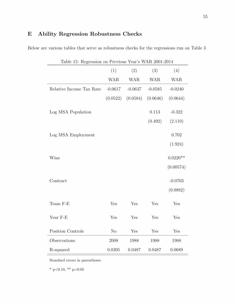
55
E Ability Regression Robustness Checks
Below are various tables that serve as robustness checks for the regressions run on Table 3
Table 15: Regression on Previous Year’s WAR 2001-2014
(1) (2) (3) (4)
WAR WAR WAR WAR
Relative Income Tax Rate -0.0617 -0.0637 -0.0585 -0.0240
(0.0522) (0.0584) (0.0646) (0.0644)
Log MSA Population 0.113 -0.322
(0.492) (2.110)
Log MSA Employment 0.702
(1.924)
Wins 0.0220**
(0.00574)
Contract -0.0703
(0.0882)
Team F-E Yes Yes Yes Yes
Year F-E Yes Yes Yes Yes
Position Controls No Yes Yes Yes
Observations 2008 1988 1988 1988
R-squared 0.0395 0.0487 0.0487 0.0689
Standard errors in parentheses
* p<0.10, ** p<0.05

56
Table 16: Regression on Previous Year’s OPS 2001-2014
(1) (2) (3) (4)
OPS OPS OPS OPS
Relative Income Tax Rate -0.00234 -0.00318 -0.00299 -0.000706
(0.00415) (0.00439) (0.00568) (0.00729)
Log MSA Population 0.00365 -0.130
(0.0711) (0.230)
Log MSA Employment 0.141
(0.237)
Wins 0.000576
(0.000799)
Contract 0.0231
(0.0151)
Team F-E Yes Yes Yes Yes
Year F-E Yes Yes Yes Yes
Position Controls No Yes Yes Yes
Observations 1100 1080 1080 1080
R-squared 0.0651 0.123 0.123 0.128
Standard errors in parentheses
* p<0.10, ** p<0.05
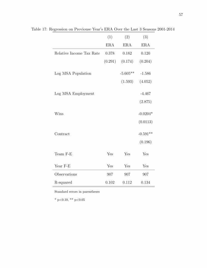
57
Table 17: Regression on Previouse Year’s ERA Over the Last 3 Seasons 2001-2014
(1) (2) (3)
ERA ERA ERA
Relative Income Tax Rate 0.378 0.182 0.120
(0.291) (0.174) (0.204)
Log MSA Population -5.605** -1.586
(1.593) (4.052)
Log MSA Employment -4.467
(2.875)
Wins -0.0204*
(0.0113)
Contract -0.591**
(0.196)
Team F-E Yes Yes Yes
Year F-E Yes Yes Yes
Observations 907 907 907
R-squared 0.102 0.112 0.134
Standard errors in parentheses
* p<0.10, ** p<0.05
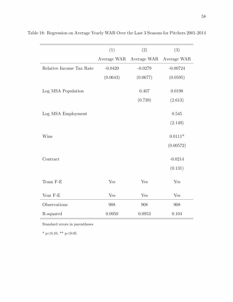
58
Table 18: Regression on Average Yearly WAR Over the Last 3 Seasons for Pitchers 2001-2014
(1) (2) (3)
Average WAR Average WAR Average WAR
Relative Income Tax Rate -0.0420 -0.0279 -0.00724
(0.0643) (0.0677) (0.0595)
Log MSA Population 0.407 0.0198
(0.739) (2.613)
Log MSA Employment 0.545
(2.149)
Wins 0.0111*
(0.00572)
Contract -0.0214
(0.131)
Team F-E Yes Yes Yes
Year F-E Yes Yes Yes
Observations 908 908 908
R-squared 0.0950 0.0953 0.104
Standard errors in parentheses
* p<0.10, ** p<0.05