tax structure and female labour market participation
TRANSCRIPT

IZA DP No. 3090
Tax Structure and Female Labour MarketParticipation: Evidence from Ireland
Tim CallanArthur van SoestJohn R. Walsh
DI
SC
US
SI
ON
PA
PE
R S
ER
IE
S
Forschungsinstitutzur Zukunft der ArbeitInstitute for the Studyof Labor
October 2007
Tax Structure and
Female Labour Market Participation: Evidence from Ireland
Tim Callan ESRI and IZA
Arthur van Soest
Tilburg University, RAND and IZA
John R. Walsh ESRI
Discussion Paper No. 3090 October 2007
IZA
P.O. Box 7240 53072 Bonn
Germany
Phone: +49-228-3894-0 Fax: +49-228-3894-180
E-mail: [email protected]
Any opinions expressed here are those of the author(s) and not those of the institute. Research disseminated by IZA may include views on policy, but the institute itself takes no institutional policy positions. The Institute for the Study of Labor (IZA) in Bonn is a local and virtual international research center and a place of communication between science, politics and business. IZA is an independent nonprofit company supported by Deutsche Post World Net. The center is associated with the University of Bonn and offers a stimulating research environment through its research networks, research support, and visitors and doctoral programs. IZA engages in (i) original and internationally competitive research in all fields of labor economics, (ii) development of policy concepts, and (iii) dissemination of research results and concepts to the interested public. IZA Discussion Papers often represent preliminary work and are circulated to encourage discussion. Citation of such a paper should account for its provisional character. A revised version may be available directly from the author.

IZA Discussion Paper No. 3090 October 2007
ABSTRACT
Tax Structure and Female Labour Market Participation: Evidence from Ireland
How great an effect does the structure of income taxes have on women’s labour market participation? This issue is investigated using a discrete choice static labour supply model for married couples in Ireland. The model incorporates fixed costs of working and simultaneously explains participation decisions and preferred hours of work. Details of the tax system are fully incorporated, and key elements of the welfare system are also taken into account. The model is estimated using data from the 1994 wave of the Living in Ireland Survey. The results are used to analyse the labour supply effects of a move to greater independence in the tax treatment of couples. The influence of tax structure on participation is reconsidered in the light of trends in women’s participation in the labour market and two key changes in the structure of taxation: a shift from a joint or aggregated basis of assessment to an “income-splitting” system in 1980 and a further substantial shift from income-splitting towards greater independence from 2000 onwards. JEL Classification: H31, J22 Keywords: labour supply, discrete choice, micro-simulation Corresponding author: Tim Callan ESRI Whitaker Square Sir John Rogerson’s Quay Dublin 1 Ireland E-mail: [email protected]

1. Introduction1
The taxation of couples is arguably “the single most important problem in personal
income taxation” (Apps and Rees, 2007). One of the critical elements in framing policy in
this area is the extent and nature of labour supply responses to alternative tax treatments of
couples. This paper investigates the influence of tax structure on the labour supply of married
women in Ireland. Since the 1960s, Ireland has moved from a system of joint taxation (with
income tax depending on aggregate income) to an income splitting system (implemented
through doubled bands and allowances for married couples) to a system with greater
independence between the taxes of husbands and wives. At the same time married women’s
labour market participation has risen from very low levels to rates close to the EU average.
We investigate the influence of tax structure on Irish women’s labour market
participation using a labour supply model based on cross-sectional data for 1994, which has
the unique advantage of incorporating information on preferred hours of work, rather than
simply actual hours. We estimate preferences within a discrete-choice structural model of
participation choices and preferred hours (see, for example, van Soest (1995) and Blundell
(2001)). Estimation is in the context of an “income-splitting” tax structure, which imposes
high marginal rates of tax on secondary earners. We then simulate the impact of tax reforms
introducing greater independence in the treatment of couples on the labour supply of both
wives and husbands. We compare the results of these reforms to the tax structure with
alternative forms of tax cut. The results are set in the context of the rise in married women’s
labour market participation in recent decades. Our model estimates the first order behavioural
labour supply effects. It does not aim at a full analysis of equilibrium effects, although the
results we obtain could be used as input for a computational general equilibrium model in
which such effects can be investigated.2
The types of tax reform that we want to consider extend beyond changing marginal
tax rates. We want to look at, for example, joint taxation of spouses versus separate taxation,
or systems which can be seen as somewhere in between these two systems. For example, we
want to look at separate filing with the possibility to transfer the tax free allowance. More
generally, we want to be able to look at complicated budget sets for two earner households,
involving non-convexities and discontinuities. Even for single persons or one-adult
households, the Irish tax-transfer system involves non-convexities, due to, for example, 1We thank participants at the LOWER conference on Women and Work for their comments; particular thanks are due to the discussant, Mareva Sabatier, 2 Recent work moving beyond the first-order impacts includes Creedy and Duncan (2005).

thresholds in social welfare premiums. We therefore need a framework which is able to deal
with complex budget sets. This makes the traditional continuous approach, developed and
surveyed by, for example, Blomquist (1983), Hausman (1985), Hausman and Ruud (1984),
and Moffitt (1986, 1990a, 1990b), inappropriate for our purposes. The traditional type of
model in principle requires budget sets which are piece-wise linear and convex. Although it is
possible to add non-convexities such as fixed costs of working (see Kapteyn et al., 1990, for
example), each non-convexity or other additional complexity of the budget set, substantially
increases the computational task of calculating the utility maximum. This becomes
particularly burdensome in the two-dimensional case, where both spouses choose their
optimal labour supply simultaneously.
This drawback can be avoided by treating the family's choice set as a finite set. For
example, instead of allowing an individual to choose any number of working hours on the
interval [0,80] (with corresponding net incomes), the assumption can be made that the
individual can only choose from the finite set {0,8,16,...,48} (with corresponding net
incomes). The choice set then consists of 7 instead of infinitely many points. The utility
maximum can be obtained directly by comparing the seven values of the (direct) utility
function in these points. Several studies have used discrete choice sets which only distinguish
between not working, part-time working, and full-time working. See, for example, Blundell
(2001), Bingley and Walker (2001), Ilmakunnas and Pudney (1990), Keane and Moffitt
(1998) and Moffitt (1984). To capture enough detail of a complex budget set with non-
convexities and discontinuities, however, a finer grid, with more than three points per
individual, seems necessary. For the one individual case, such models have been widely used
by, for example, Dickens and Lundberg (1993), Tummers and Woittiez (1991), and van Soest
et al. (1990). Van Soest (1995) analyses a discrete choice model for family labour supply.
Refinements of his model, for example allowing for fixed costs of working, and using
information on actual as well as desired hours of work, have been introduced in, for example,
Callan and van Soest (1996), Creedy et al. (2006), Euwals and van Soest (1999) and Haan
(2006).
The current paper uses a discrete choice model of this latter type. We focus on
married couples. We assume that the two spouses have a common utility function.3 The
function arguments are family income, leisure of the husband, and leisure of the wife. We
3 See Vermeulen (2006) for a comparison of this approach with collective models where each spouse has their own utility function.. See Beblo et al. (2004) for a micro-simulation model based upon a collective approach.
3

will use a direct quadratic utility function, which is easy to interpret and can deal with
negative incomes (which can arise due to fixed costs), while it also has the desirable property
of local second order flexibility.
We allow for preference variation across households through observed as well as
unobserved characteristics. This is achieved by making several parameters of the utility
function dependent on characteristics such as age and family composition, and a random error
term. Moreover, we add independent error terms to the values of the utility function at all
alternatives in the choice set, with the same specification as in the multinomial logit model.
To explain why there are relatively few people with a part-time job, we incorporate
fixed costs of work. These fixed costs are again allowed to depend upon observed and
unobserved characteristics of the family and its members. The fixed costs are fully integrated
in the structural model: they are subtracted from family income if someone works, and thus
enter the utility function through income. Increasing fixed costs reduces income if someone
works, and will thus make not working relatively more attractive compared to working.
We assume that before tax hourly wage rates do not vary with hours worked. This
assumption is maintained in most of the neoclassical labour supply models, although some
exceptions exist, such as Moffitt (1984), Tummers and Woittiez (1991), and Ilmakunnas and
Pudney (1990). Thus each individual is assumed to have a unique before tax wage rate.
Together with hours worked and the tax system, the before tax wage rate determines net
earnings. A common problem in labour supply models with non-workers is that wage rates of
non-workers are not observed. To account for this, a wage equation is estimated, and wage
predictions are constructed for non-workers. Due to the non-linear nature of the labour supply
model, however, replacing wage rates by their predictions leads to inconsistent estimates,
even if the wage predictions themselves are unbiased. To account for this, wage rate
prediction errors are explicitly incorporated in the model, as additional unobserved error
terms.
The labour supply model is based upon the assumption that individuals or couples
maximize (joint) utility, and thus aims at estimating preferences of those who supply labour.
It is therefore estimated using information on preferred hours of work, so that deviations
between preferred and actual hours of work - due to, for example, involuntary unemployment
or a lack of part-time jobs - are allowed for.
The questions on preferred hours of work in our data do not explicitly state whether or
not the spouse is also assumed to change to his or her optimum. We will assume that each
individual’s answer is based on the assumption that the spouse also adjusts to the family
4

optimum. An alternative would be to assume that the spouse is constrained at his or her actual
number of hours, but incorporating this into the model would require joint modelling of
actual and desired hours of both spouses. This is beyond the purpose of the current paper.
To account for the various unobserved error terms, the model is estimated with
simulated maximum likelihood (with correction for the selective nature of the second
sample): the likelihood function is replaced by an approximation based upon simulation, and
the simulated approximation of the likelihood is maximized. The estimator is asymptotically
equivalent to exact maximum likelihood.
The data we use are from the 1994 wave of the Living in Ireland Panel Survey. This is
a representative household panel containing about 1,300 married couples in the age group 18
to 65. The results are used to analyse the sensitivity of labour supply for wages, and to
analyse the first order labour supply effects of a proposed reform of the tax system. This is
done by means of simulations. First, participation rates and average hours worked are
computed on the basis of the estimates and the actual wages and tax rules. Second, the
simulation is repeated for various alternative scenarios. The first scenario is that all wage
rates of husbands or wives are raised by the same percentage. This leads to estimates of own
and cross wage elasticities of both spouses.
The focus of the simulations is the analysis of labour supply effects of changing the
income tax rules. For the data period (and for many years before and after) the Irish tax
system could be characterized as embodying “income splitting”, though technically this was
implemented by affording double allowances and rate bands to married couples.4 This system
is commonly seen as a disincentive for married women to join the labour market, since the
secondary worker (usually the wife) faces the higher marginal tax rate of the primary worker
(the husband). We will analyse the possible labour supply effects of changing to an
individualized tax system.
The structure of the remainder of this paper is as follows. Section 2 describes the data.
The labour supply model is discussed in Section 3. In Section 4, we discuss the results and
the labour supply elasticities. Section 5 discusses the actual Irish income tax system and the
proposed reforms. In Section 6 we discuss the outcomes of our simulation analysis of the
labour supply effects of these reforms. Section 7 concludes.
4 Cohabiting couples did not benefit from this treatment: they were treated as single persons by the tax system, but in a similar fashion to married couples by the welfare system. There were only a small number of cohabiting couples in the survey, and they were excluded from the present analysis.
5
2. Data Survey respondents are quite commonly asked about their actual hours of work in the
paid labour market. But actual hours worked do not always represent the individual’s
preferred hours of work. For example, an individual may wish to work fewer hours, but
cannot obtain part-time work with similar conditions to the full-time job. On the other hand,
an individual may find him- or herself unemployed, but may wish to obtain a full-time job
and be actively searching for one. Labour supply models which ignore this fact, and treat
actual hours as identical with desired hours, are likely to be imperfect guides to labour market
behaviour. In attempting to identify the impact of taxes and net wages on labour supply
decisions, there are considerable advantages to be gained from working with information on
individual’s preferred hours of work. In the Irish context, such information is available from
the 1994 wave of the Living in Ireland survey (LII), which for this reason is the dataset
employed here.5 The survey, the Irish element of the European Community Household Panel,
has been widely used in studies of poverty, income distribution and the labour market and has
been found to be broadly representative of the Irish population. (For a full description of the
data, including checks on its general representativeness, see Callan et al. 1996).
The basic information used to construct the preferred hours variable comes from a
number of questions, depending on the labour market status of the individual concerned. For
those who are in employment, and working in a paid job for more than 15 hours per week (a
cut-off imposed by the design requirements of Eurostat), the information comes from the
answer to the question: Suppose that you could continue to work in your present job, and could choose exactly how many hours to work. Your hourly rate of pay would not change, but your total weekly pay would vary depending on how many hours you worked. How many hours per week would you like to work? (Living in Ireland, 1994 Questionnaire, question A.39) For those who are either unemployed or seeking other work to replace or in addition to a job
of less than 15 hours per week, preferred hours are taken as the answer to the question: If you could find a suitable job, how many hours per week would you prefer to work in this new job? (Living in Ireland, 1994 Questionnaire, question D.2)
5 There have, of course, been considerable changes in the Irish labour market since then, most notably a rise in female participation rates, a fall in unemployment and a substantial increase in total employment. It seems likely, however, that these changes are associated more with changes in the opportunities facing individuals than with a sharp change in preferences. This suggests that results such as those obtained here – identifying preferences and examining the likely response to alternative policy experiments – have a strong continuing relevance.
6

If, however, the individual is not seeking work – for reasons which could include study,
training, housework, caring for children or others, retirement, personal illness or injury – then
preferred hours are taken as being zero.
For those working less than 15 hours per week, and not seeking additional work, there are
two other possibilities, based on the response to the question: What is your MAIN reason for working less than full-time? (Living in Ireland, 1994 Questionnaire, q. C.5) If such a worker states that the main reason is that “I want but cannot find a full-time job”
then preferred hours are set equal to 40 (the modal value for full-time workers). But other
reasons (such as being in education/training, caring for children or others, personal illness or
disability, not wanting a full-time job) lead to actual hours being taken as the best indication
of preferred hours.
Table 1: Criteria Defining the Sample used for Labour Supply Analysis
Criterion No. of cases excluded No. of cases remaining
Married couple, both aged 65, not in full-time education, with responses to individual questionnaire 2,260 Exclude: Self-employed, farmer 696 1,564 Exclude: Cases with missing values 165 1,399 Exclude: Ill or disabled 87 1,312 Exclude: Persons exiting a job 16 1,296 Final sample 1,296
Table 1 sets out the criteria used to identify the sample on which the model was to be
estimated. The survey contained responses from 2,260 married couples where both partners
were aged under 65 and neither partner was in full-time education.6 Almost 700 couples were
excluded from the analysis because at least one spouse was engaged in farming or other self-
employment. This is because the labour supply choices facing the self-employed are rather
different, and even the measurement of hours of work and the financial return from work
become more difficult. While this is a very common exclusion in the international literature
6 In principle, cohabiting couples could also have been included in the analysis, provided that the rules governing their tax liabilities and welfare entitlements could also have been modelled. The small potential increase in sample size did not warrant the considerable additional time and effort which would have been required at this stage. The issues involved could be revisited with a dataset incorporating a larger number of cohabiting couples.
7

on labour supply, it affects proportionately more cases in the Irish context – particularly
because of the higher rate of participation in farming. The remaining exclusions – of cases
with missing information on variables needed for the analysis, of couples including a person
classifying his or her labour force status as “ill or disabled”,7 and of persons who at the time
of interview were leaving a job – amount to about 270 cases. The final sample for analysis
includes information on 1,296 couples.
Tables 2, 3 and 4 set out basic descriptive statistics on the variables used in the
analysis. We note some key features of the hours and wages variables below. On average,
husbands are in paid employment for almost 32 hours per week, as against 10 hours per week
for wives. This gap is only partly accounted for by a lower rate of labour market participation
among women. For those in paid employment, there is still a substantial gap (42 hours per
week for men and 28 for women). On average men’s preferred hours of work were greater
than their actual hours (36 hours as against 32 hours per week), but women’s preferred hours
of work were slightly lower than their actual hours (10 hours as against 11 hours per week).
Figure 1 shows the distribution of preferred hours of work for husbands and wives in
paid employment. There is a sharp “spike” in preferred hours for men at about 40 hours per
week, with almost 60 per cent of all those with positive preferred hours indicating that this is
their preferred situation. By contrast, the distribution of preferred hours for married women is
bi-modal, with less sharp peaks at both 20 and 40 hours. Almost 80 per cent of women with
positive preferred hours wish to work for less than 40 hours, with a considerable spread over
the different hours categories. Just under half of married men and just over 70 per cent of
married women have actual hours of work which are approximately equal to their preferred
hours of work.
Gross hourly wages are constructed by dividing the usual gross wage per week or per
month by the usual number of hours worked during the relevant pay period. The gross wage
of employed married women in the 1994 sample was Ir£6.90, or about three-quarters of the
average wage for married men (Ir£9.04). Figure 2 illustrates the distribution of gross hourly
wages for men and women in paid employment. Around 44 per cent of married women had
an hourly gross wage of less than Ir£5 in 1994, as against only 15 per cent of married men.
7 Other persons with an illness or disability hampering daily activity are included, and this information on their illness/disability status is used in the analysis.
8

Table 2: Variable definitions and sample statistics
Variable and unit of measurement Minimum Maximum Mean Standard Deviation
Preferred hours per week — husband 0 80.0 35.8 14.1 — wife 0 65.0 11.1 14.7 Usual hours in all jobs per week — husband 0 100.0 31.8 20.2 — wife 0 84.0 10.0 15.6 Gross wage (Ir£ per hour) — husband 0 54.8 6.82 5.99 — wife 0 26.7 2.41 4.22 Potential experience (years) — husband 3.9 52.1 28.1 11.0 — wife 0.4 52.6 26.2 10.8 Husband’s highest educational qualification: None beyond primary 0 1 0.364 0.481 Group Certificate 0 1 0.106 0.309 Intermediate/Junior Certificate 0 1 0.141 0.348 Leaving Certificate 0 1 0.212 0.409 Diploma 0 1 0.052 0.223 University degree/higher degree 0 1 0.123 0.329 Wife’s highest educational qualification None beyond primary 0 1 0.360 0.480 Group Certificate 0 1 0.052 0.223 Intermediate/Junior Certificate 0 1 0.186 0.389 Leaving Certificate 0 1 0.291 0.454 Diploma 0 1 0.046 0.209 University degree/higher degree 0 1 0.065 0.246 Big town 0 1 0.520 0.500 City 0 1 0.407 0.491 Dublin 0 1 0.309 0.462 Age of husband (years) 23.3 65.0 44.7 10.4 Age of wife (years) 19.1 65.0 42.7 10.1 Illness/disability hampering daily activity — husband 0 1 0.122 0.327 — wife 0 1 0.138 0.345 Child in 0-4 Age Bracket? (0=no, 1=yes) 0 1 0.279 0.449 Child in 5-12 Age Bracket? (0=no, 1=yes) 0 1 0.471 0.499 Number of children aged under 18 0 9 1.74 1.50 Occupational pension (Ir£/week) — husband 0 759.0 8.5 44.6 — wife 0 161.0 0.4 6.6 Mortgage interest (Ir£/week) 0 163.8 20.5 25.6 Investment income (Ir£/week) — husband 0 143.8 2.2 9.9 — wife 0 126.2 0.5 4.3 No. of children eligible for Child Benefit 0 8 1.62 1.45 Notes: Number of cases 1,296
9

Table 3: Distribution of family size
No. of children aged under 18 % of couples None 26.6 1 19.2 2 24.8 3 18.7 4 6.9 5 or more 3.8 All 100.0
Table 4: Descriptive statistics for nonzero cases
Variable
Nonzero cases as % of all cases Minimum Maximum Mean
Std. Deviation
Preferred hours — husband 89.6 1 80 39.9 7.6 — wife 41.7 3 65 26.5 10.4 Usual hours in all jobs — husband 75.4 2 100 42.1 10.1 — wife 34.9 2.5 84.0 28.6 13.0 Gross hourly wage (Ir£/hour) — husband 75.4 1.6 54.8 9.04 5.24 — wife 35.0 0.8 26.7 6.90 4.47 Occupational pension (Ir£/week) — husband 5.2 7.2 759.0 161.3 116.2 — wife 0.4 30.4 161.0 93.7 56.8 Mortgage interest 63.3 0.1 163.8 32.5 25.5 Investment income (Ir£/week) — husband 25.2 <0.05 143.8 8.6 18.3 — wife 10.7 <0.05 126.2 4.6 12.5 Figure 1: Distribution of Preferred Hours of Work for Husbands and Wives in Paid Employment, 1994
10
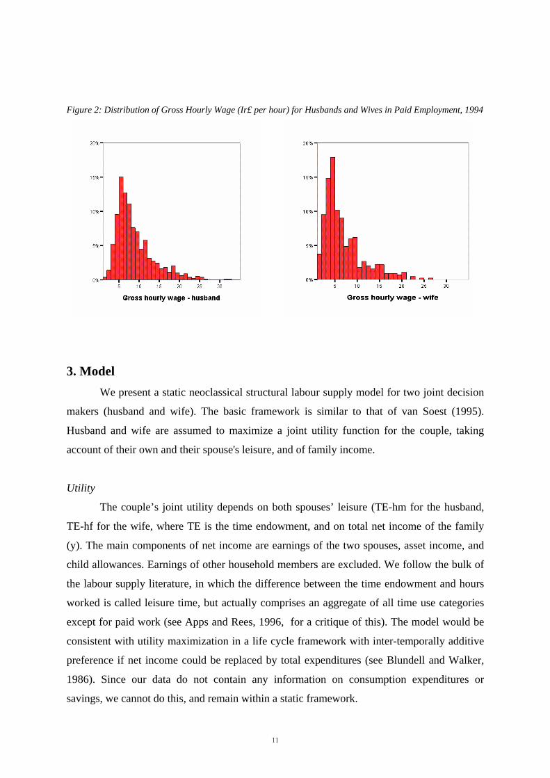
Figure 2: Distribution of Gross Hourly Wage (Ir£ per hour) for Husbands and Wives in Paid Employment, 1994
3. Model We present a static neoclassical structural labour supply model for two joint decision
makers (husband and wife). The basic framework is similar to that of van Soest (1995).
Husband and wife are assumed to maximize a joint utility function for the couple, taking
account of their own and their spouse's leisure, and of family income.
Utility
The couple’s joint utility depends on both spouses’ leisure (TE-hm for the husband,
TE-hf for the wife, where TE is the time endowment, and on total net income of the family
(y). The main components of net income are earnings of the two spouses, asset income, and
child allowances. Earnings of other household members are excluded. We follow the bulk of
the labour supply literature, in which the difference between the time endowment and hours
worked is called leisure time, but actually comprises an aggregate of all time use categories
except for paid work (see Apps and Rees, 1996, for a critique of this). The model would be
consistent with utility maximization in a life cycle framework with inter-temporally additive
preference if net income could be replaced by total expenditures (see Blundell and Walker,
1986). Since our data do not contain any information on consumption expenditures or
savings, we cannot do this, and remain within a static framework.
11

We use a quadratic direct utility function:8
U(v) = v'Av + b'v, v=(y, (80-hm), (80-hf))' (1)
Without loss of generalization, the time endowment has been set to 80 hours per
week. Another choice of the time endowment or a specification in terms of hours worked
instead of leisure, would give exactly the same model. The specification in terms of leisure is
chosen to simplify the interpretation of the results. Without restrictions on the parameters,
this utility function is locally second order flexible. In principle there is no reason to prefer
this utility function to any other direct utility function with the same (or larger) flexibility.
Van Soest (1995), for example, uses a direct utility function which is quadratic in log income
and log leisure of both spouses (direct translog). This has the drawback that it cannot deal
with negative incomes, which imposes restrictions on the way in which fixed costs can be
incorporated (see below).
We impose parameter restrictions to guarantee that utility increases with income,
since this is necessary for the economic interpretation of the model.9 For a similar reason, we
will impose that utility decreases with leisure of both spouses. We do not impose quasi-
concavity of preferences and thus avoid the critique by MaCurdy et al. (1990).
In the specification of the direct utility function in (1), A is a 3x3 matrix of unknown
parameters and b is a three-dimensional vector. We assume that b2 and b3 depend on
individual or household characteristics, i.e. we allow for variation of preferences across the
sample through observed characteristics:
bk = X k 'βk + υk k=2,3, (2)
Here the Xk are vectors of observed characteristics (log age and log age squared of
husband (in b2) or wife (in b3), a dummy for health problems of husband (in b2) and wife (in
b3), number of children, and a dummy for the presence of children younger than 6). The error
terms υk (k=2,3) represent unobserved characteristics, reflecting unobserved heterogeneity of
preferences. We will discuss assumptions concerning their distributions below.
8 The index for the household is suppressed. 9 This is achieved by penalizing the likelihood. An alternative would be to use a less flexible utility function, such as CES (see Vlasblom, 1998).
12

Husband and wife are assumed to maximize the same utility function. The labour
supply decision is thus modelled at the household level, as in, for example, Hausman and
Ruud (1984) and Van Soest (1995). A more general framework would be a game theoretic
model with different utility functions for the two spouses (see Kooreman and Kapteyn, 1990,
for example). This is beyond the purpose of the current paper.
Constraints
The answer to the question: "how many hours would you like to work?" is based upon
utility maximization under constraints. An obvious constraint is the budget restriction: to
each choice of the number of working hours of husband and wife corresponds a different net
income. To determine net income as a function of working hours of both spouses, we need
earnings of both spouses, other household income (child benefits, asset income), taxes,
potential unemployment assistance and other social security benefits. Other household
income is always observed and can therefore directly be drawn from the data. To determine
earnings for each number of working hours for each spouse, we assume that gross hourly
wage rates do not depend on hours worked (see Section 1). For workers with observed wage
rate, we can then compute gross earnings for each possible number of working hours.
For non-workers, we need to predict the before tax wage rate. For this purpose, we
have estimated wage equations for men and women, accounting for selection bias in the usual
way (see Heckman, 1979). The estimates of the wage equations are then used to predict the
wages of non-workers. Because the labour supply model is nonlinear in wages, it is necessary
to take the wage rate prediction errors into account to get consistent estimates of the labour
supply model (see the description of the estimation technique given below).
To determine social security benefits in case of working few or zero hours, we take
account of the basic system of unemployment assistance only. This is relatively easy to
model: families are entitled to social assistance if family income falls below the minimum
standard of living, which depends on age, marital status and family composition (we ignore
the fact that these unemployment assistance benefits are means tested). We do not model
unemployment insurance benefits. This is difficult to model due to lack of data and due to the
static nature of our framework, since unemployment insurance benefits are of a temporary
nature.
Following Van Soest (1995), the budget constraint under which the individual
maximizes utility will be approximated by a finite number of points. In our benchmark
model, we take multiples of 8 hours (0,8,..,48) for each individual. This gives 49 points for
13

the couple. We will analyse the sensitivity of our results for the number of points we use. The
vectors appearing in the utility function are denoted by vj:
vj = (yj, 80-hmj, 80-hfj)' (j=1,...,49)
where yj is net family income in the situation where the husband works hmj hours per week,
and the wife works hfj hours per week.
There are two ways to interpret the answer to the preferred hours question (see
Section 2). The first corresponds to unrestricted optimization of family utility. In this case,
the husband’s and wife’s preferred hours yield the vector vj which maximizes utility over the
full set of 49 points. The second interpretation is that each spouse answers the preferred hours
question taking the partner’s hours as given. This would correspond to restricted optimization
under the constraint that the partner’s hours are equal to their actual hours. In this case the
husband’s and wife’s preferred hours correspond to potentially different vj, which both
maximize utility in a set of only seven points. In either case, utility maximization is
straightforward. First order conditions etc. are not required; the choice set is finite. We
estimate and simulate the model for the first interpretation. An estimation procedure based on
the alternative interpretation of the answers to the “preferred hours” question gave rise to
similar estimates of labour supply elasticities. The main reason for working with the
unrestricted optimisation interpretation is that policy simulations can then be performed
without considering actual hours. Our policy simulations focus on the effect of taxes on
desired hours. If desired hours also depend on (the spouse’s) actual hours, a policy simulation
would also require an analysis of the response of actual hours to changes in desired hours.
Alternative-specific error terms
The only error terms included so far are random preferences. In addition, we
introduce alternative specific error terms as follows:
u(vj) = U(vj) + εj
We assume that the εj are iid and follow an extreme value distribution. We assume that the
answer to the desired hours question is based upon maximizing u(vj) rather than U(vj). The εj
can be seen as the error made in evaluating alternative j. There are several reasons why these
14
errors are incorporated. First, they are needed to give nonzero probability to choices which
cannot be optimal for any value of the random preferences. Such choices may very well exist
in case of a nonconvex or discontinuous budget set, where some points on the budget frontier
may give very low family income compared to adjacent points. In this sense, they play the
same role as the optimization or measurement errors in the Hausman (1985) model. The
second reason for including the εj is computational: we will see below that they facilitate
simulated maximum likelihood estimation. In this sense they function as a smoothing device.
The same interpretation is given to them by Keane and Moffitt (1998). They use the same
type of error terms, though they impose that the error terms have a small variance compared
to the remaining part of u(vj) - an assumption we do not make. Third, the εj can be interpreted
as alternative specific unobserved characteristics of each offered alternative (Aaberge et al.,
1999).
Due to the assumption on the distribution of the εj the resulting model shows some
similarity to the multinomial logit model. The probability that an individual chooses
alternative j, conditional on wage rates, tax and benefit rules, exogenous variables, and
random preference parameters, is given by:
P[j] = exp{U(vj )}/∑k exp{U(vk)} (3)
Given our interpretation of the desired hours question, the combination of desired hours of
both spouses (hmj, hfj) reflects the family optimum, and the summation in (3) is over all 49
points in the family choice set. Other interpretations of the desired hours questions would
imply that the summation is over a smaller set.
P[j] increases with U(vj) (for given values of the other U(vk)). Since U is increasing in
income, the utility of working increases with the (before and after tax) wage rate. The utility
of non-participation does not depend upon the wage rate. As a consequence, the participation
probability increases with the wage rate. On the other hand, the participation probability
decreases with the benefits level: a higher benefits level increases the utility level if a benefit
is received, but does not affect utility values of the alternatives where working hours are so
large that benefit income is zero.
15

Fixed costs of working
The model described so far typically under-predicts the number of non-workers. A
possible explanation is that there are fixed costs of working. In other words, there is a gain to
not working compared to all the other possibilities, which makes not working more attractive
than working few hours per week. The level of the fixed costs may depend on individual and
household characteristics Xk (k=2,3) We model them as:
FCk = X'αk+ηk, k=2 (husband) and k=3 (wife)
Here the Xk are the same family and individual characteristics as in the utility function (see
(2)), and ηk are error terms reflecting unobserved heterogeneity in fixed costs. In computing
the values of the utility function, we replace income yj by yj - FC2 if according to alternative
j the husband works, by yj - FC3 if the wife works, and by yj - FC2 - FC3 if, for alternative j,
both husband and wife work. Since U is increasing with income, positive fixed costs increase
the utility of not working compared to the utility of not working. They thus make working
less attractive, and decrease the probability of participation.
If we used log income in the utility function, negative values of income corrected for
fixed costs could not be handled. With normally distributed random errors ηk, this problem
would occur with positive probability. In such cases, censoring family income to a small
positive value would be necessary. This can be seen as a drawback of the quadratic in logs
specification, which we avoid by using the quadratic in levels specification.10 Fixed costs
were also used by Callan and van Soest (1996) and Euwals and van Soest (1999). Another
possibility to explain the lack of part-time jobs is to model the availability of part-time jobs
using job offer probabilities. This implies that the choice set varies across households, with a
common probability distribution for all households in the sample. This approach is followed
by Dickens and Lundberg (1993), Woittiez and Tummers (1991), and van Soest et al. (1990).
While this may be plausible for actual hours, it seems less appropriate for explaining
preferred hours, which should not be affected by availability constraints. Van Soest (1995)
used disutilities of part-time jobs, assumed to be independent of family characteristics. These
disutilities reflect search costs of jobs with irregular hours. Again, for explaining preferred
hours this seems less plausible. 9 In the quadratic in logs utility function model, this problem could be avoided by modelling fixed costs multiplicatively, but this seems less plausible from an economic point of view.
16

Distribution of error terms
The error terms in the model are the alternative specific errors εj, the random
preference terms υk (k=2,3), the unobserved heterogeneity in fixed costs ηk (k=2,3), and the
error terms in the wage equations (ζk , k=2,3, say). We already made the assumption that the
εj follow an iid generalised extreme value distribution. The other error terms are assumed to
be normal with mean 0. We assume that all the error terms are independent of the covariates
in X2 and X3 and of the regressors in the wage equations. For identification and
computational convenience, we assume that all the error terms are independent of each other,
with some exceptions: we allow for a non-zero correlation between ζ2 and υ2 and between ζ3
and υ3. One reason for such a correlation may be “division bias” in wage rates, which can
arise because the hourly wage is calculated as the ratio of gross pay to hours worked in the
period; see Gong and van Soest (1998), who find in a model for female labour supply that
such a correlation is significant, and not allowing for it leads to a downward bias in the wage
elasticity estimate.11
To incorporate the correlations between ζj and υj (j=2 (men), 3 (women)), we
implement the random preference terms in the following way (where all N(0,1) draws are
independent of each other and of everything else):
Let ej(w) be either the standardised residual from the wage equation (if the wage
is observed) or an N(0,1) draw (if the wage is unobserved)
Let ej(rp) be an N(0,1) draw
The random preference term υ2 is generated as Φujej(rp) + λ wjej(w)
The parameters Φuj and λwj are estimated jointly with all the parameters (see Table 5).
Estimation
Due to the multinomial logit nature of the model, estimation by maximum likelihood
would be straightforward if all wages and all random preference terms and fixed costs
heterogeneity terms were observed. In that case, the likelihood would follow directly from
(3), since the vj would then be known functions of parameters, explanatory variables, and
observed error terms ηk, ζk and υk (k=2,3). Since we do not observe these error terms (except
those in the wage equations for workers – for given parameter values, they can be computed 11 We have also experimented with a non-zero correlation between husband’s and wife’s random preference terms υ2 and υ3, to allow for flexible substitution patterns. This correlation, however, appears hard to estimate with any reasonable level of accuracy, and we find that setting it to zero hardly affects the other results.
17

as residuals from the wage equation), the likelihood contribution is not simply given by (3).
Instead, it is given by the mean value of the appropriate expression according to (3), with the
mean taken over the unobserved errors. Since there are between four and six unobserved
errors, this implies that a four to six dimensional integral is needed. Approximating such an
integral by conventional numerical (quadrature) routines is time consuming and intractable. A
more convenient alternative is simulated maximum likelihood: the integral is replaced by a
simulated average based upon R independent draws from the (multivariate normal)
distribution of the unobserved errors (conditional upon the residuals in the equations of the
observed wages, if any). Due to the law of large numbers, the approximation will be accurate
if R becomes large. With independent draws across households, it can be shown that the
approximation is accurate enough to make simulated maximum likelihood asymptotically
equivalent to exact maximum likelihood if R tends to infinity faster than the square root of
the number of observations (see, e.g., Hajivassiliou and Ruud, 1994). In our benchmark
model we use R=20 draws per household. We have examined the sensitivity of our results for
the choice of R, and find that there is little variation for values of R between 20 up to 100
The simulated maximum likelihood procedure is greatly facilitated by the presence of
the εj. Without these, the likelihood contribution conditional on the unobserved error terms
would be either 0 or 1. The simulated likelihood would become a discontinuous function of
the parameters, its maximization would be numerically much harder, and zero contributions
would have to be dealt with. Adding the εj smoothes the likelihood and bounds it away from
zero. Adding the εj could thus be seen as a smoothing device, without giving the εj any real
economic meaning. This is the interpretation of McFadden (1989) and Keane and Moffitt
(1998). In both of these articles, the variance of the εj is fixed at some small value, while at
the same time, a normalization is imposed on the systematic part of the utility function. This a
priori limits the share of the variance of the εj in the total variance of u(vj). We normalize the
variance of εj only, and do not impose an additional normalization on the utility function.
Thus we avoid imposing a priori that the εj should play only a minor role. This corresponds to
the view that the εj could have some meaning as alternative specific errors in the economic
model. We let the data decide how important this is.
4. Results The benchmark model has a choice set of 49 points for each family, where each
spouse can choose between 0, 8,...., 48 hours per week. It is estimated using R=20 simulated
18

maximum likelihood replications for each observation. The parameter estimates are shown in
Table 5. The upper panel refers to the terms in the utility function. The index m denotes the
husband and f denotes the wife. A positive coefficient on one of the interactions with leisure
(i.e. one of the β-s in b2 and b3, see (2)) implies a positive effect on the marginal utility of
leisure and thus a negative effect on labour supply. For both spouses, age is significant, and
the age pattern of preferred hours is decreasing with age, particularly for older individuals.
The presence of children has a strong negative effect on the wife's labour supply. For the
husband, however, preferred hours increase significantly with the number of children, ceteris
paribus. The presence of young children (age 0-5) reduces labour supply of women, and is
insignificant for men. Men who suffer from an illness hampering daily activity have
significantly lower preferred hours than healthy men, ceteris paribus. For women, the health
dummy has the same sign, but the effect is much smaller and insignificant at the 5% level.
Fixed costs of working depend on the same individual and family characteristics as
preferences. The estimates imply that average fixed costs amount to the equivalent of about
€59 per week for me and about €160 per week for women (in 1994 prices). Particularly the
latter amount seems quite large, and would imply negative family incomes if both spouses
had part-time jobs. It should be kept in mind, however, that fixed costs are unobserved, and
will comprise any incentive for not working, including non-monetary incentives. For
example, the lack of attractive small part-time jobs and the difficulty in finding a part-time
job might induce people not to work and indicate not working as their preferred labour
market state. In our model, this will be picked up as fixed costs of working also. The
estimated standard deviations on the error terms in the fixed costs equations (equivalent to
€47 for men and €123 for women) show that a substantial part of the fixed costs are not
explained. They also imply that for many respondents, fixed costs do not play a role at all.
For both spouses, the age pattern of fixed costs is U-shaped, with a minimum at about
age 40. For women, the children variables have the expected sign. The number of children is
significant at the 5% level, while, the dummy for young children is significant at the 10%
level only. Still, the point estimates suggest that the added fixed costs of working for women
due to a young child are about three to four times larger than the additional fixed costs due to
an older child. For the husbands’ fixed costs of working, children do not play a role. The
illness dummy has the expected positive sign for both spouses. Somewhat surprisingly
perhaps, its effect is larger and more significant for women than for men.
19

Table 5: Estimated Parameters for Direct Utility Function and Fixed Costs in ModellingPreferred Hours of Work
Variable Coefficient Standard error t-statistic
Direct utility function (Income/100)2 -0.253 0.032 -7.89 (Husband’s leisure/10) 2 -0.364 0.045 -8.15 (Wife’s leisure/10) 2 -0.358 0.040 -8.91 (Income*Husband’s leisure)/1000 0.316 0.027 11.67 (Income*Wife’s leisure)/1000 0.073 0.018 4.09 (Husband’s leisure*Wife’s leisure/100) 0.080 0.018 4.33 Income/100 1.468 0.560 2.62 Husband’s leisure/10 46.10 11.14 4.14 (Husband’s leisure/10)* ln(Husband’s age) -25.51 5.97 -4.27 (Husband’s leisure/10)* ln(Husband’s age)2 3.646 0.798 4.57 (Husband’s leisure/10)* Husband has illness? 0.514 0.119 4.32 (Husband’s leisure/10)* No. of children -0.123 0.031 -3.91 (Husband’s leisure/10)* Child under 5? 0.084 0.115 0.73 Wife’s leisure hours/10 23.97 10.39 2.31 (Wife’s leisure/10)*ln(Wife’s age) -13.19 5.73 -2.30 (Wife’s leisure/10)*ln(Wife’s age)2 2.080 0.787 2.64 (Wife’s leisure/10)*Wife has illness? 0.199 0.134 1.48 (Wife’s leisure/10)*No. of children 0.117 0.037 3.15 (Wife’s leisure/10)*Child under 5? 0.391 0.109 3.58 Fixed costs – husband const_fc/100 28.86 10.54 2.74 ln (Husband’s age) -15.90 5.62 -2.83 ln (Husband’s age)2 2.214 0.747 2.96 Husband has illness hampering activity?
0.197 0.109 1.81
Number of children eligible for Child Benefit -0.025 0.030 -0.84 Child aged under 5?
-0.060 0.121 -0.49
Fixed costs – wife const_fc/100 19.77 12.20 1.62 ln (Wife’s age) -11.06 6.69 -1.65 ln (Wife’s age)2 1.610 0.913 1.76 Wife has illness hampering activity? 0.361 0.147 2.46 Number of children eligible for Child Benefit 0.093 0.044 2.12 Child aged under 5?
0.268 0.131 2.05
Error terms (See section 3) ση2 0.342 0.064 5.36 ση3 1.007 0.102 9.84 Φu2 0.164 0.083 1.96 Φu3 0.008 0.105 0.08 λw2 0.399 0.048 8.33 λw3 0.279 0.047 5.95 Note: Variables involving a question (denoted by ?) are dummy variables, with values 1 for a
“Yes” and 0 for a “No”..
20

For both men and women, we find a significantly positive covariance between the
error term in the wage equation and the random preference term in the marginal utility of
leisure. For women in particular, the correlation is quite strong and the correlation coefficient
is close to 1. Since the marginal utility of leisure is negatively related to labour supply, this
implies a negative correlation between errors in wage equation and labour supply equation.
This is in line with the division bias explanation for the correlation between these error terms.
Elasticities
With models of this type, the parameter estimates do not directly reveal the sensitivity
of labour supply for financial incentives. In particular, (uncompensated) elasticities for both
spouses’ wage rates will be the main driving force behind the tax policy effects. To compute
these, we have carried out some simulations. The individual elasticities vary across the
sample. Since we want to use the model for policy analysis, we are mainly interested in
aggregate elasticities. We define the (own or cross) wage elasticity of labour supply of some
given group of people (husbands or wives) as the percentage change in total desired hours of
that group if all before tax wage rates (of husbands or wives) in that group rise by 1%.
While this definition is a widely-used one in the analysis of labour supply, “labour supply
elasticity” has a wide variety of other meanings. Many studies only consider the elasticities
for the average (“representative”) family. In a highly non-linear model like ours, these
elasticities are not necessarily very informative for the consequences of wage changes for a
heterogeneous population. Another approach is to consider average elasticities instead of
elasticities of the average. The average elasticity can be seen as a weighted aggregate
elasticity of hours worked, where more weight is given to people with lower desired hours.
Other studies look at elasticities of hours worked conditional upon participation. For policy
analysis, however, the effect on participation is at least as important as the effect on hours
worked given participation, particularly for married women, whose participation rate is below
50 per cent. We compute elasticities taking full account of the (positive) impact of the wage
rate on the participation decision (with desired hours equal to zero for non-participants).
Actually, our results suggest that most of the sensitivity of labour supply for wage rates is
driven by changes in the decision to participate. Elasticity calculations can also vary in the
way in which the tax system is accounted for. We change all gross wage rates by 1 per cent
and leave the tax system unaffected. The way in which net wage rates change is thus not
fixed a priori, but driven by the existing tax system. On average, after tax wage rates will
change by slightly less than 1 per cent, due to the progressive nature of the tax rules. In the

case of family labour supply, elasticities vary with what is assumed about the spouse’s
income and behavioural response. In line with the model introduced in Section 3, we assume
that both spouses jointly adjust to the new family optimum; but similar results were found
under the alternative assumption that each partner answered the question about desired hours
on the assumption that their spouse’s hours would not change.
For men, we find an own wage elasticity of 0.25. That is, if all gross wage rates of the
men in our sample increased by 1%, while women’s wage rates remained unchanged, men’s
total desired hours would increase by 0.25% (with a 95 per cent confidence interval from
0.21% to 0.30%). Most of the effect is due to increased participation: a rise in the gross wage
rates of all husbands of 1% would induce an increase in the number of men willing to
participate of almost 0.2 percentage points, i.e. 0.21% of the actual participation rate of
almost 90%. For women, the estimated own wage elasticity is 0.83 (confidence interval from
0.71 to 0.90). The elasticity of the participation rate is 0.49 and thus again explains the largest
part of the labour supply elasticity. These estimates are in line with other findings for Ireland
(e.g, Doris, 2001) and with the broad range of empirical findings of labour supply elasticities
for other countries (see Blundell and MaCurdy, 1999), even though, as explained above, a
comparison is hampered by the fact that the large number of empirical studies are based on an
almost as large number of elasticity concepts.
Table 6: Labour supply elasticities for married men and married women with respect to wage changes
Elasticity of average preferred hours to change in wages
Change in: Husbands Wives
Male wage 0.25 -0.35 Female wage -0.07 0.83 Both wages 0.18 0.48 Note: A 1 per cent rise in the male wage leads to a 0.25 per cent rise in average preferred hours of married men, and a fall of 0.35 per cent in the average preferred hours of married women.
We find cross wage elasticities of –0.07 for men and –0.35 for women. As a
consequence, if all wage rates of both men and women increased by 1%, the model predicts
that desired hours would rise by 0.25-0.07=0.18% for men and by 0.48% for women.
The analysis deals with desired or preferred hours of work at the wage rate the
individual currently commands. This allows for considerable simplification over analyses
22

which must deal with the potential for involuntary unemployment or actual hours of work
which diverge from preferred hours. It can also be seen as allowing for maximum flexibility
in labour market response. In some circumstances changes in desired hours will not translate
into changes in actual hours because of constraints on individual behaviour (e.g., having to
choose between full-time and part-time work; or being involuntarily unemployed).
Nevertheless, it is of interest that the own-wage elasticities for men and women reported by
Callan and van Soest (1996), based on 1987 data on actual hours and incorporating modelling
of involuntary unemployment and constraints on hours, are quite similar to those reported
here (0.15 for men, 0.67 for women)
5. Tax Treatment of Couples Over time a number of countries have moved from systems involving “income-
splitting” or extensive transferability of allowances between spouses to systems involving
greater independence in the tax treatment of husband and wives – and, correspondingly, more
restricted transferability of allowances and/or bands.12 More recently the Irish tax system has
moved towards greater independence in the tax treatment of couples, in what has been termed
“individualisation” of the standard rate tax band. There has been considerable speculation
about the likely impact of this change on the participation of married women in the paid
labour market. Analysis of the type set out here is necessary to provide estimates of likely
impacts which can be used to inform the debate.
The Irish tax system – like the UK system – initially treated married couples as a unit
for income tax purposes, with the wife’s income being aggregated along with that of her
husband. While there was a “married man’s allowance”, tax was assessed on the basis of the
same band width as for single persons. Compared to two cohabiting single persons, a married
couple received a marriage subsidy if the wife was not earning an independent income, or
earned a very low one. But if the wife’s earnings were greater, she, and the couple, faced a
substantial tax penalty – a married couple with both partners in employment could face a
much higher tax bill than an unmarried couple in identical circumstances.
The Supreme Court ruled that this feature of the tax system was unconstitutional. A
number of responses to this ruling may have been possible. The one chosen by the
government, and implemented in Budget 1980, was to allow doubled rate bands and doubled
12 See OECD, 1977 and O’Donoghue and Sutherland (1999) The latter found that 10 out of 15 EU countries had income tax systems which were based around independent or individual taxation of husbands and wives.
23

allowances to all married couples. Formally, this was equivalent to allowing “income
splitting,” i.e., calculating the couple’s tax liability on the basis of assigning half the income
to each partner and taxing them as if they were single. It was also equivalent to full
transferability not only of allowances but also of rate bands. Married couples were permitted
to minimise their tax liabilities by assigning allowances and rate bands freely to either
partner. This structure operated from 1980 up to 2000, so it is the system which obtained
when the 1994 data were collected.
The Budget for the year 2000 introduced a move towards greater independence of
taxation, by means of what was termed “individualisation” of the standard rate tax band. This
involved restricting the extent to which tax bands are transferable between spouses. In 1999
the standard rate band was Ir£14,000 for an individual, or Ir£28,000 for a couple i.e., a non-
earning partner could transfer 100% of his or her tax band (and, indeed, of his/her allowance).
In 2000, full transferability of tax allowances remained as before, but there were, in effect,
restrictions on the transferability of the standard rate band. The band for a single person was
increased from Ir£14,000 to Ir£17,000 per annum; for a married couple with one income the
band remained unchanged at Ir£28,000 per annum; but the band for a married couple, both
earning, rose to Ir£34,000 (twice the single band, thereby meeting the requirement of “no
marriage penalty”). Thus, in effect, only two thirds [(28,000-17,000)/17,000=11/17] of a non-
earning partner’s band was transferable.13 The stated objective was to arrive at a position
after three years where each individual, whether single or married, has his/her own standard
rate tax band which can be set off against his/her own income but cannot be transferred
between spouses. By December 2001 the proportion of the band which was transferable had
fallen to about one-third, remaining at that level after Budget 2003.
In what follows, we model a very similar policy change, with transferability of
allowances being maintained, but transferability of rate bands removed. This has the incipient
effect of raising tax revenues. We examine two revenue-neutral approaches. In one, the
incipient revenue gain is returned to households in the form of an increase in child benefit –
reflecting the fact that the main justification for the income-splitting policy (given in the
Budget speech for the year 1979) was to provide support for families with children.
Alternatively, revenue neutrality could be attained by an across the board cut in taxes. In both
13 In the immediate aftermath of the budget, a special Home Carer’s Allowance was introduced for couples with one partner staying at home to care for a child or children, an elderly person or someone with a disability.
24

cases there are substantial reductions in the effective marginal tax rates facing second earners
in a couple.
6. Simulating the Labour Supply Impact of Tax Reforms
In this section we analyse the first order labour supply effects of the tax reform
proposal described above. Our structural model is particularly useful to do this, since it
accounts for the complete structure of the tax system, including non-convexities. Moreover,
the model predicts the effects on participation as well as the distribution of hours worked.
The way in which the effects are predicted is very similar to the method of computing the
elasticities in Section 4. Using the parameter estimates, we first predict labour supply using
the actual 1994 tax rules. We then repeat the simulation using the tax rules after the reform.
Comparing the two outcomes gives the predicted changes. For the simulation after the
reform, we assume that before tax wage rates remain the same. Thus general equilibrium
effects are not taken into account: we consider the first order effects only.14
Table 7 shows the impact of alternative ways of implementing increased
independence in the tax treatment of husbands and wives. Option (A) simply involves the
elimination of transferability of the standard rate tax band, and would generate something
about Ir£210m per annum in extra tax revenue.15 Option (B) returns this revenue to taxpayers,
via proportionate cuts in the standard and top tax rates. Option (C) is also revenue neutral, but
the incipient rise in revenue is used to fund an increased child benefit.
A notable feature of option (A) is that it gives rise to a net increase in labour market
participation (a fall in married men’s participation being more than offset by a rise in the
participation of married women), while at the same time actually increasing net revenue for
the Exchequer. Options (B) and (C), returning this revenue via general tax cuts or via child
benefit, are designed to be approximately revenue neutral.16 Option (B), combining non-
transferable bands with cuts in tax rates, gives rise to a sharp rise in married women’s
participation, and leaves men’s participation almost unchanged. Option (C), using the
revenue from restrictions on transferability to fund an increased child benefit, also boosts
married women’s participation, but leads to a fall in men’s participation.
14 Our results can in principle serve as input for a macro-economic general equilibrium type of model based upon micro foundations. 15 All calculations are undertaken in a 1994 setting. 16 As noted earlier, this is revenue neutrality on a static basis; increases (falls) in participation/hours would give rise to increased (reduced) revenues.
25

Table 7: Response of Husbands’ and Wives’ Participation Rates to Increased Independence in Tax
Treatment of Married Couples Change in tax structure % point change
in husbands’ participation rate
% point change in wives’
participation rate
Net change in Exchequer revenue as estimated by
SWITCH on full sample17
(A) Standard rate band made non-transferable
-0.5
+1.8
+Ir£210m
(B) Band non-transferable, tax rates cut to 25.4% and 45.1%
-0.1
+2.6
-Ir£8m
(C) Band non-transferable, Child Benefit increased by 69%
-0.9
+1.6
+Ir£1m
What about the total labour supply response, in terms of desired hours of work?
Under option (A), the rise in average desired hours of work for women is almost offset by a
fall in desired hours for men. Under option (B), which includes a significant cut in tax rates
as well, the response of married women is more positive, and that of married men is less
negative. As a result, the overall labour supply response for married couples is positive – and
the response of single people, not simulated here in the present framework, would also be
positive. Under option (C), the gain in tax revenue arising from non-transferability is applied
to fund a rise in child benefit. This gives rise to a fall in male labour supply which is only
partially offset by a rise in the labour supply of married women.
How do these results compare with the labour supply impact of simply cutting tax
rates, or increasing tax free allowances (the “zero rate band”)? We simulated the impact of
alternative forms of tax cut on labour supply. Table 8 shows the impact on participation rates,
which again is the driving force in the overall change. The cost of each tax cut was calibrated
to be about €250m, which could finance a cut of close to 3 percentage points in the standard
rate of tax (initially 27 per cent) or a cut of 6 percentage points for the higher rate. It is clear
that the impact on married women’s participation in the labour market of the change in tax
treatment of couples is substantially greater than for each of these forms of tax cut. The
overall labour supply impact of the structural package based on a revenue-neutral tax cut is
also greater than that of a 30% increase in the standard rate band or a 20% increase in the
personal allowance (zero rate band).
17 In euro terms, the exchequer costs were about €266m, €10m and €1.3m for options A, B and C respectively.
26
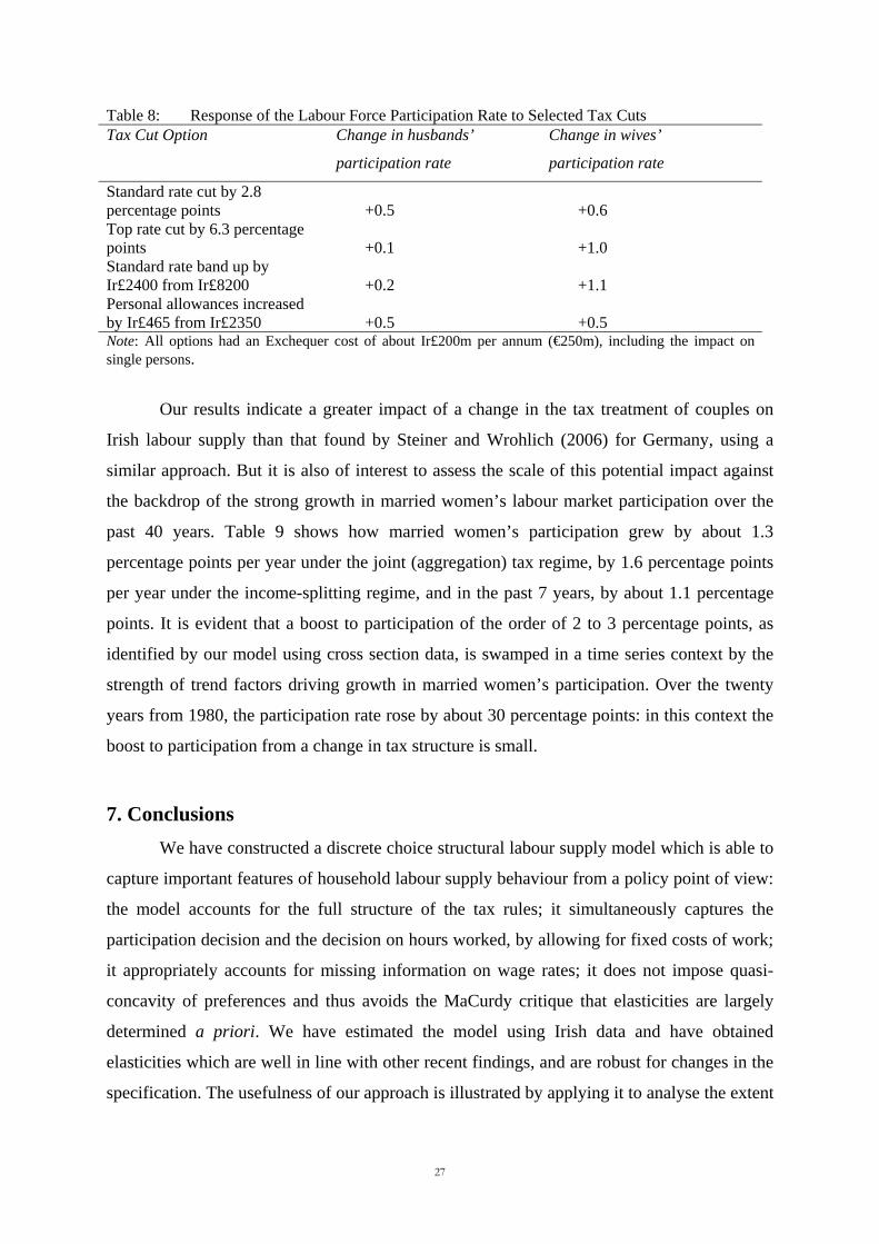
Table 8: Response of the Labour Force Participation Rate to Selected Tax Cuts Tax Cut Option Change in husbands’
participation rate
Change in wives’
participation rate
Standard rate cut by 2.8 percentage points
+0.5
+0.6
Top rate cut by 6.3 percentage points
+0.1
+1.0
Standard rate band up by Ir£2400 from Ir£8200
+0.2
+1.1
Personal allowances increased by Ir£465 from Ir£2350
+0.5
+0.5
Note: All options had an Exchequer cost of about Ir£200m per annum (€250m), including the impact on single persons.
Our results indicate a greater impact of a change in the tax treatment of couples on
Irish labour supply than that found by Steiner and Wrohlich (2006) for Germany, using a
similar approach. But it is also of interest to assess the scale of this potential impact against
the backdrop of the strong growth in married women’s labour market participation over the
past 40 years. Table 9 shows how married women’s participation grew by about 1.3
percentage points per year under the joint (aggregation) tax regime, by 1.6 percentage points
per year under the income-splitting regime, and in the past 7 years, by about 1.1 percentage
points. It is evident that a boost to participation of the order of 2 to 3 percentage points, as
identified by our model using cross section data, is swamped in a time series context by the
strength of trend factors driving growth in married women’s participation. Over the twenty
years from 1980, the participation rate rose by about 30 percentage points: in this context the
boost to participation from a change in tax structure is small.
7. Conclusions
We have constructed a discrete choice structural labour supply model which is able to
capture important features of household labour supply behaviour from a policy point of view:
the model accounts for the full structure of the tax rules; it simultaneously captures the
participation decision and the decision on hours worked, by allowing for fixed costs of work;
it appropriately accounts for missing information on wage rates; it does not impose quasi-
concavity of preferences and thus avoids the MaCurdy critique that elasticities are largely
determined a priori. We have estimated the model using Irish data and have obtained
elasticities which are well in line with other recent findings, and are robust for changes in the
specification. The usefulness of our approach is illustrated by applying it to analyse the extent
27

to which changes in the tax treatment of couples may boost married women’s labour market
participation.
We consider a reform to the tax treatment of couples, making their taxes more
independent and thereby reducing marginal tax rates on second earners. Our model identifies
a labour supply impact that is larger than those for quite substantial cuts in taxes, and much
larger than those found by Steiner and Wrohlich (2006) using similar methods for Germany.
However they are small in relation to the strong trend growth in married women’s
participation.
Table 9: Married women’s labour market participation rate, and tax treatment of couples, 1971-2007
Year Joint Income-splitting Quasi-independent
1971 7.5% 1977 14.4% 1979 17.9% 1981 16.7% 1987 23.4% 1989 23.7% 1991 30.2% 1992 32.5% 1993 34.5% 1994 36.0% 1995 37.7% 1996 40.9% 1997 41.5% 1998 43.2% 1999 44.9% 2000 45.9% 2001 46.6% 2002 48.0% 2003 48.3% 2004 49.2% 2005 51.3% 2006 52.4% 2007 53.5%
28
References
Aaberge, R., U. Colombino and S. Strom (1999), Labour Supply in Italy: An Empirical
Analysis of Joint Household Decisions, with Taxes and Quantity Constraints, Journal
of Applied Econometrics, 14(4), 403-422.
Apps, P.F. and R. Rees (1996), Labour supply, household production and intra-family
welfare distribution, Journal of Public Economics, 90, 199-219.
Apps, P.F. and R. Rees (2007) “The Taxation of Couples”, IZA Discussion Paper No. 2910.
Beblo, M., D. Beninger and F. Laisney (2004), Family Tax Splitting: A Microsimulation of
Its Potential Labour Supply and Intra-household Welfare Effects in Germany, Applied
Economics Quarterly, 50(3), 233-250.
Blomquist, N.S. (1983), The effect of income taxation on the labour supply of married men in
Sweden, Journal of Public Economics, 22, 169-197.
Bingley, P. and I. Walker (2001), Housing Subsidies and Work Incentives in Great Britain,
Economic Journal, 111(471), C86-103.
Blundell, R. (2001), Welfare reform for low income workers, Oxford Economic Papers, 53,
190-214.
Blundell, R. and I. Walker (1986), A life-cycle consistent empirical model of family labour
supply using cross-section data, Review of Economic Studies, 80, 539-588.
Blundell, R. and T. MaCurdy (1999), “Labor supply: A review of alternative approaches”, in:
O. Ashenfelter and D. Card (eds.), Handbook of Labor Economics Vol. 3,
Amsterdam: Elsevier
Callan, T. and A. van Soest (1996), “Family labour supply and taxes in Ireland”, ESRI
Working Paper No. 78.
Callan, T., B. Nolan, B.J. Whelan, C.T. Whelan and J. Williams (1996), Poverty in Ireland in
the 1990s: Evidence from the Living in Ireland Survey, Dublin: Oaktree Press.
Creedy, J. and A. Duncan (2005), Aggregating labour supply and feedback effects in
microsimulation, Australian Journal of Labour Economics, 8(3), 277-290.
Creedy, J., G. Kalb and R. Scutella (2006), Income distribution in discrete hours behavioural
microsimulation models: An illustration, Journal of Economic Inequality, 4, 57-76.
Dickens, W. and S. Lundberg (1993), Hours restrictions and labor supply, International
Economic Review, 34, 169-192.
Doris, A. (2001), “The Changing Responsiveness of Labour Supply During the 1990’s,” in
Quarterly Economic Commentary, December, Dublin: ESRI, pp. 68-82.
29

Euwals, R. and A. van Soest (1999), Desired and actual labour supply of unmarried men and
women in the Netherlands, Labour Economics, 6, 95-118.
Gong X, van Soest A (2002) Family structure and female labor supply in Mexico City.
Journal of Human Resources, 37, 163–191.
Haan, P. (2006), Much ado about nothing: Conditional logit vs. random coefficient models
for estimating labour supply elasticities, Applied Economics Letters, 13(4), 251-256.
Hajivassiliou, V. and P. Ruud (1994), “Classical estimation methods for LDV models using
simulation,” in: R. Engle and D. McFadden (eds.), Handbook of Econometrics, vol.
IV, North-Holland, New York, pp. 2384-2443.
Hausman, J. (1985), The Econometrics of nonlinear budget sets, Econometrica, 53, 1255-
1283.
Hausman, J. and P. Ruud (1984), Family labor supply with taxes, American Economic
Review 74, 242-248.
Heckman, J. (1979), Sample selection bias as a specification error, Econometrica 47,
153-161.
Ilmakunnas, S. and S. Pudney (1990), A model of female labour supply in the presence of
hours restrictions, Journal of Public Economics, 41, 183-210.
Kapteyn, A. P. Kooreman and A. van Soest (1990), Quantity rationing and concavity in a
household labour supply model, The Review of Economics and Statistics, 70(1), 55-
62.
Keane, M. and R. Moffitt (1998), A structural model of multiple welfare program
participation and labor supply, International Economic Review, 39, 553-589.
Kooreman, P. and A. Kapteyn (1990), On the empirical implementation of some game
theoretic models of household labor supply, Journal of Human Resources, 25, 584-
598.
MaCurdy, T., D. Green, and H. Paarsch (1990), Assessing empirical approaches for
analyzing taxes and labor supply, Journal of Human Resources, 25, 415-490.
Moffitt, R. (1984), Estimation of a joint wage-hours labor supply model, Journal of Labor
Economics, 2, 550-556.
Moffitt, R. (1986), The econometrics of piecewise linear budget constraints: a survey and
exposition of the maximum likelihood method, Journal of Business and Economic
Statistics, 4, 317-327.
Moffitt, R. (1990a), The econometrics of kinked budget constraints, Journal of Economic
Perspectives, 4, 119-139.
30

Moffitt, R. (1990b), Special issue on taxation and labor supply in industrial countries,
Journal of Human Resources, 25, 313-558.
O’Donoghue, C. and H. Sutherland (1999), Accounting for the family in European income
tax systems, Cambridge Journal of Economics, 23(5), 565-598.
OECD (1977), The treatment of family units in the OECD member countries under tax and
transfer systems, Paris: OCDE.
Steiner, V. and K. Wrohlich (2006) “Introducing family tax-splitting in Germany: How
would it affect the income distribution and work incentives?”, IZA Discussion Paper
No. 2245.
Tummers, M. and I. Woittiez (1991), A simultaneous wage and labor supply model with
hours restrictions, Journal of Human Resources, 26(3), 393-423.
Van Soest, A., I. Woittiez and A. Kapteyn (1990), Labour supply, income taxes and hours
restrictions in the Netherlands, Journal of Human Resources, 25, 517-558.
Van Soest, A. (1995), Discrete choice models of family labor supply, Journal of Human
Resources, 30, 63-88.
Vermeulen, F. (2006), A collective model for female labour supply with non-participation
and taxation, Journal of Population Economics, 19(1), 99-118.
Vlasblom, J.D. (1998), Differences in labour supply and income of women in the Netherlands
and the Federal Republic of Germany, PhD thesis, University of Utrecht.
31