TAX POLICY AND HOUSING INVESTMENT IN AUSTRALIA

Mark Britten-Jones Warwick J. McKibbin Reserve Bank of Australia The Brookings Institution

Research Discussion Paper

8907

November 1989

Research Department

Reserve Bank of Australia

This paper has benefited from some unpublished work by Eric Siegloff on housing investment in the MSG model. We thank Matthew Jones, Malcolm Edey and colleagues at the Reserve Bank for helpful discussions and comments. The views expressed are those of the authors and do not necessarily reflect the views of the The Brookings Institution or the Reserve Bank of Australia.

ABSTRACT

This paper develops a simulation model of the Australian housing market which incorporates many of the important features of housing. The use of an intertemporal framework allows us to examine the relationship between house prices, land prices, rental return on housing and investment in housing. We use the model to examine the consequences for the housing market of the removal of the capital gains tax, a cut in income tax rates, a rise in real interest rates and an increase in the rate of goods price inflation. One key result is that changes in the inflation rate will cause changes in real prices and in housing investment even when real interest rates and demand are constant. This is due to the distortions caused by taxing and allowing tax deductions based on nominal interest. We simulate a policy change where the tax base is altered so that tax is levied on real interest only and find that under this regime real prices and activity are not influenced by changes in the inflation rate.

1

TABLE OF CONTENTS

ABSTRACT 1

TABLE OF CONTENTS . . . . . . . . . . . . . . . . . . . . . . . . . u

1. Introduction . . . . . . . . . . . . . . . . . . . . . . . . . . . . . . . 1

2. Model Structure . . . . . . . . . . . . . . . . . . . . . . . . . . . 2 a. General Features . . . . . . . . . . . . . . . . . . . . . . . 3 b. Supply . . . . . . . . . . . . . . . . . . . . . . . . . . . . . . 3 c. House Prices . . . . . . . . . . . . . . . . . . . . . . . . . 10 d. Demand . . . . . . . . . . . . . . . . . . . . . . . . . . . . 11

3. Numerical Solution of the Model . . . . . . . . . . . . . . . 12

4. Simulation Results . . . . . . . . . . . . . . . . . . . . . 15 a. Removal of Capital Gains Tax on Housing 18 b. Cut in Company Tax Rate by 10 Percent . 18 c. Replacing Nominal Interest Deductibility by Real

Interest Deductibility . . . . . . . . . . . . . . . . . . . . 18 d. Permanent 300 Basis Point Rise in Real Interest

Rates . . . . . . . . . . . . . . . . . . . . . . . . . . . . . . 22 e. Permanent 5 Percent Rise in Inflation . . . . . . . . . 22 f. Permanent 5 Percent Rise in Inflation with only Real

Interest Deductibility. . . . . . . . . . . . . . . . . . . . . . 22

5. Conclusion 25

APPENDIX I 27

APPENDIX II . . . . . . . . . . . . . . . . . . . . . . . . . . . . . . . 28

APPENDIX III 31

APPENDIX IV 32

REFERENCES 33

ll

TAX POLICY AND HOUSING INVESTMENT IN AUSTRALIA

Mark Britten-Jones and Warwick J. McKibbin

1. INTRODUCTION

The housing market is frequently the focus of economic debate especially during periods of rapidly rising housing prices. Recently, Albon (1989) and others have questioned the efficiency of the tax advantages given to housing investment in Australia although rigorous modelling of the Australian housing market has been scarce. Nevile et al. (1987) incorporate the effects of taxation in a static housing model. Such a model is silent about the level of housing investment induced by tax changes and the resultant effects on rent levels, given changes in the stock of housing.

The purpose of this paper 1s to develop a d ynarnic intertemporal model of the housing sector that can be used to analyse the effects on housing investment, housing prices. land prices and rents, of various tax policies.

In the model we develop here, the level of housing investment is based on investment decisions by forward-looking managers (investors) who maximise the value of the firm subject to increasing adjustment costs. Under this framework, taxes and interest rates affect the profitability and market value of capital in the housing sector. This causes changes in desired investment levels as well as prices. The specification is a synthesis of the q theory of investment of Tobin (1969), the adjustment cost framework of Abel (1982) and the tax policy analysis of Hall and Jorgenson (1967). The specification of adjustment dynamics follows the approach forn1alised by Hayashi (1982).

The model employed here has several attractive features which extend previous studies in this area. Firstly it is a two factor model (land and capital). This allows us to discuss land prices

2

which are an important component of house prices. Secondly we take care to pay attention to the Australian taxation system. In particular the model incorporates a real capital gains tax as well as depreciation allowances and the tax deductibility of nominal interest costs. The analysis includes the various tax rules relevant to homeowners and landlords and it accounts for the influence of these costs on rental prices, house prices and land prices as well as the stock of houses.1

Section 2 of the paper describes the model and its development from the optimisation problem of a representative investor. The model is then calibrated to Australian data in section 3 and we discuss the technique used to solve the model. In section 4 we use numerical simulation techniques to examine the effects, both on the steady state of the model as well as the transition path between steady states, following changes in tax policy, inflation and interest rates. A summary and conclusion is contained in section 5.

2. MODEL STRUCTURE

The housing sector has several unique characteristics. These characteristics include heterogeneity, durability, spatial fixity, and the extensive role of government both directly (e.g. public housing) and indirectly (e.g. housing specific taxes and subsidies). In this model the heterogeneity of housing is dealt with by assuming the existence of an unobservable homogeneous commodity called housing services. The durability of housing is dealt with by assuming that one homogeneous unit of housing stock yields one unit of housing services per unit time. Spatial fixity means that location is a characteristic of the housing stock. This characteristic is ignored in our model so that we may concentrate on the effects of government taxes and subsidies. In particular, the model includes the effects of debt financing and inflation -

1The major limitation of the model is that it is driven by investors to the exclusion of owner-occupants. This is an area for further extension of the model. The role of investors in the housing market is discussed in Section 2b.

3

"negative gearing", the capital gains tax, and the different tax treatment of owner-occupants versus investors.

The housing market also has several complex intertemporal features. At any point in time, the housing stock depends on past flows of housing investment; housing investment depends on expected returns to housing which will in turn depend on future rents. Future rents are not only determined by housing demand but also by the future housing stock. The intertemporal framework employed in our n1odel incorporates all these feedback effects. This framework permits a rigorous dynamic analysis of tax policy and changes in tax policy.

a. General Features

The model has two factors of production, land and capital. The representative agent is a firm which supplies housing services. A unit of housing services is produced by one unit of housing stock. The firm purchases land and capital and installs the capital on the land to produce a stock of houses which provides a flow of housing services. Although we analyse the costs of home ownership and the value of a house to an owner-occupant, the model does not explicitly incorporate owner-occupants. Demand is modelled very simply allowing attention to be focused on taxes and the supply side of the housing market.

The model incorporates considerable detail on taxes. The discount factor is an after-tax cost of capital. Tax is paid on earnings and depreciation allowances are generated by investment in housing structures. We model the real capital gains tax by assuming that capital gains tax is paid as the real capital gain occurs. The tax concessions and value of a house to owner-occupants are analysed under various assumptions about future inflation rates and financing arrangements. We also simulate the introduction of tax-deductibility only applying to the real component of interest pay1nents.

b. Supply

The representative agent is considered to be a firm (housing investor) that installs houses on land that it has purchased and

4

then rents these house/land packages (henceforth called homes) out to derive income. Our justification for using this approach is twofold.

Firstly if there are any firms operating in the above manner in the housing market then, given our assumption of homogeneity, the resulting marginal conditions which we derive will apply across the whole housing sector. Marginal decisions by investors will affect and determine the prices within the whole housing sector given levels of demand by renters. If this were not the case, housing investors would enter or exit up until the point at which these marginal conditions are fulfilled. Thus because housing investors under the current tax regime constitute a significant force in the housing market, it is appropriate to model their behaviour as being representative of the whole market.

Secondly, although similar marginal conditions apply to owner­occupants the conditions involve marginal utilities which are unobservable. Investors, however, base their decisions on variables which are more easily observed or inferred, e.g. rental return and price appreciation. For this reason investor behaviour is more amenable to analysis than the behaviour of owner-occupants.

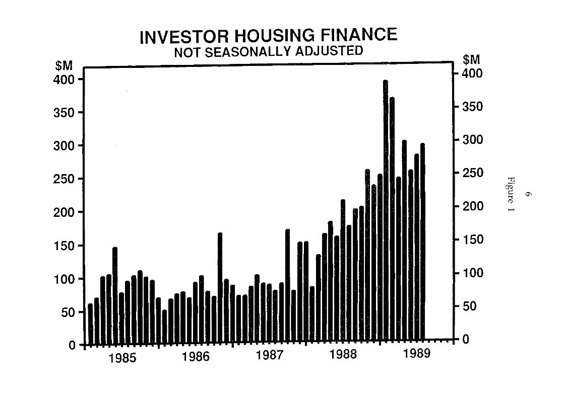
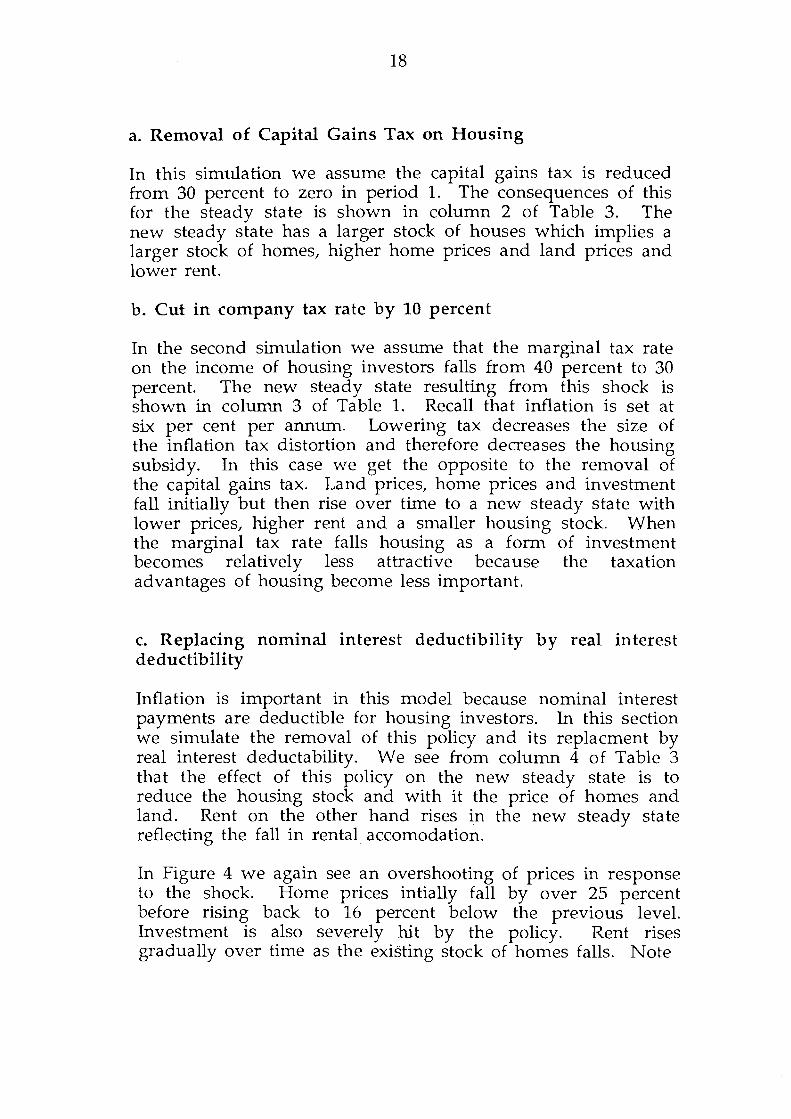
In the first three months of 1989 investors paid $1.7 billion for established dwellings. This compares with the $4.1 billion paid by owner-occupants. Thus, empirically, investors constitute a significant force in the housing market. Note that in Figure 1 the loans to investors for the purchase of dwellings increased dramatically at the end of 1987 when the current tax regime involving negative gearing was reintroduced.

The firm is a price-taker in both the capital rnarket and the product market, and incurs adjustment costs with respect to housing investment. It faces a corporate tax system that includes depreciation allowances and the tax deductibility of interest payments. There is no uncertainty in the modet and the firm's planning is done under perfect foresight. Therefore the finn acts to maximise the present value of future after-tax cash flows, discounted at the nominal after-tax cost of capital i, which is assu1ned constant. Formally we can write the value of the finn to be maximised as:

5

00

r p R e-i(s-t)ds ) s ... 's (1)

t

where V is the present value of future after tax cash flows, P 5

is a price index, ~ is real after tax cash flows in period s and i is an after tax cost of capital. We can think of the nominal interest rate as being composed of two parts, an inflation premium 1t and a real component r. The corporate tax rate is u so the after-tax cost of capital is (1-u)(1t + r). However, we introduce the possibility of the inflation component being taxed at a different rate g. The after-tax cost of capital is then,

i = (1-u)r + (1-g)7t (2)

Real after-tax cashflow ~ is written as after-tax revenue plus a depredation tax deduction less expenditures on land and housing investment,

(3)

where p5 is real pre-tax revenue in period s, L B is the amount of land bought at a real price pL and ~ is the real present value at time s of the tax bill saving due to depreciation deductions on a dollar of investment in housing structures in period s. ~ is the amount of gross investment expenditure on housing structures with a price PHs in period s.

Real pre-tax revenue Ps is written as:

Ps = PHSF(K,L) (4)

where pHS is the real pnce of home services or m more familiar wording, rent. F is the production function, K the stock of housing structures and L the stock of land. The production function is Cobb-Douglas with constant returns to scale. We assume that rates and other expenses are zero.2

2 These could easily be incorporated but do not add anything to the questions on which we focus in this study.

$M 400

350

300

250

200

150

100

50

0

-•

•

•

----

1985

INVESTOR HOUSING FINANCE NOT SEASONALLY ADJUSTED

II

1986 1987 1988

-"'"

~

--

-""

-. .

1989

$M 400

350

300

250

200

150

100

50

0

"T:1 .......

~ (J"\ '-t ro 1--'

7

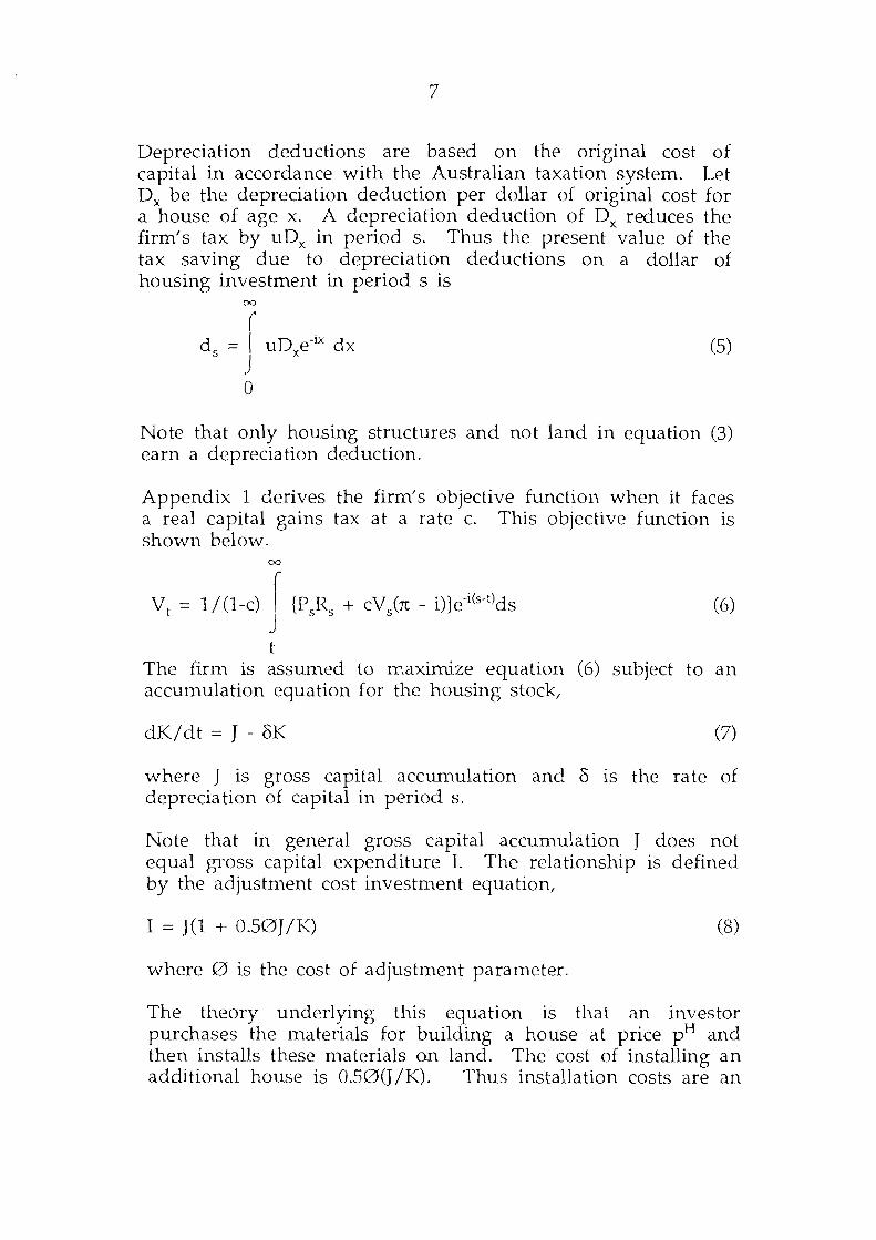
Depreciation deductions are based on the original cost of capital in accordance with the Australian taxation system. Let Dx be the depreciation deduction per dollar of original cost for a house of age x. A depreciation deduction of Dx reduces the firm's tax by uDx in period s. Thus the present value of the tax saving due to depreciation deductions on a dollar of housing investment in period s is

00

( d := I uDxe-ix dx

s j (5)

0

Note that only housing structures and not land in equation (3) earn a depreciation deduction.

Appendix 1 derives the firm's objective function when it faces a real capital gains tax at a rate c. This objective function is shown below.

00

Vt = 1/(1-c) r (P5R

5 + CV

5(TC - i)}e·i(s-t)ds

j (6)

t The firm is assumed to rnaximize equation (6) subject to an accumulation equation for the housing stock,

dK/dt = J - 8K (7)

where J is gross capital accun1ulation and 8 1s the rate of depreciation of capital in period s.

Note that in general gross capital accumulation J does not equal gross capital expenditure I. The relationship is defined by the adjustment cost investment equation,

I = J(l + 0.50J /K) (8)

where 0 is the cost of adjustment parameter.

The theory underlying this equation is that an investor purchases the 1naterials for building a house at price pH and then installs these materials on land. The cost of installing an additional house is 0.50(J /K). Thus installation costs are an

8

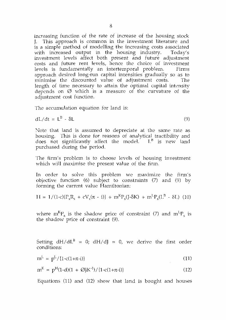
increasing function of the rate of increase of the housing stock J. This approach is common in the investment literature and is a simple method of modelling the increasing costs associated with increased output in the housing industry. Todays investment levels affect both present and future adjustment costs and future rent levels, hence the choice of investment levels is fundamentally an intertemporal problem. Firms approach desired long-run capital intensities gradually so as to 1ninimise the discounted value of adjustment costs. The length of time necessary to attain the optimal capital intensity depends on 0 which is a measure of the curvature of the adjustment cost function.

The accumulation equation for land is:

dL/dt = LB - oL (9)

Note that land is assumed to depreciate at the same rate as housing. This is done for reasons of analytical tractibility and does not significantly affect the model. L B is new land purchased during the period.

The firm's problem is to choose levels of housing investment which will maximise the present value of the firm.

In order to solve this problem we maximize the firm's objective function (6) subject to constraints (7) and (9) by forming the current value Hamiltonian:

where mKP5

is the shadow price of constraint (7) and mLP5

is the shadow price of constraint (9).

Setting dH/ dL B = 0; dH/ dJ = 0, we derive the first order conditions:

(12)

Equations (11) and (12) show that land is bought and houses

9

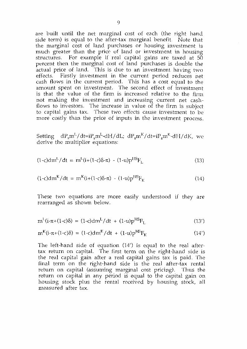
are built until the net m.arginal cost of each (the right hand side term) is equal to the after-tax marginal benefit. Note that the marginal cost of land purchases or housing investment is much greater than the price of land or investment in housing structures. For exarnple if real capital gains are taxed at 50 percent then the marginal cost of land purchases is double the actual price of land. This is due to an investment having two effects. Firstly investment in the current period reduces net cash flows in the current period. This has a cost equal to the amount spent on investm.ent. The second effect of investment is that the value of the firm is increased relative to the finn not making the investment and increasing current net cash­flows to investors. The increase in value of the firm is subject to capital gains tax. These two effects cause investment to be more costly than the price of inputs in the investment process.

Setting dP5mL/dt=iP5mL-dH/dL; dP

5mK/dt=iP

5mK-dH/dK, we

derive the multiplier equations:

(13)

(14)

These two equations are more easily understood if they are rearranged as shown below.

mL(i-n+(l-c)8) = (1-c)dmL I dt + (l-u)pH5FL

mK(i-n+(l-c)8) = (1-c)dmK /dt + (l-u)pH5FK

(13')

(14')

The left-hand side of equation (14') is equal to the real after­tax return on capital. The first term on the right-hand side is the real capital gain after a real capital gains tax is paid. The final term on the right-hand side is the real after-tax rental return on capital (assuming marginal cost pricing). Thus the return on capital in any period is equal to the capital gain on housing stock plus the rental received by housing stock, all measured after tax.

10

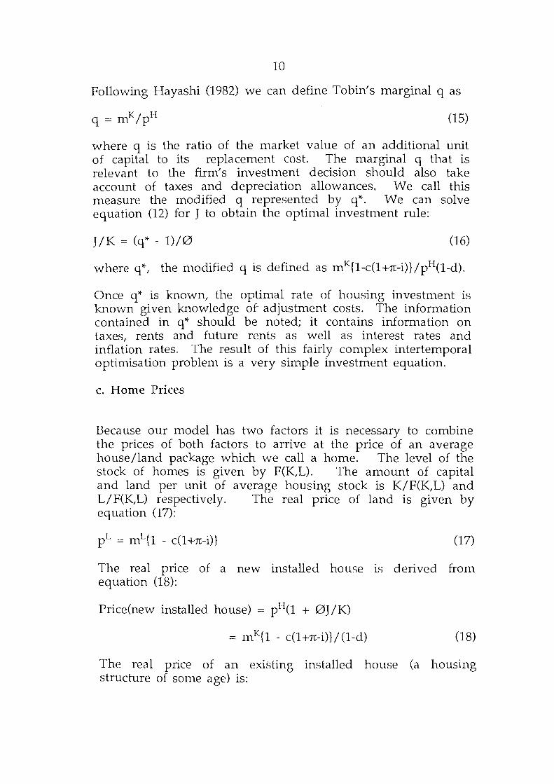
Following Hayashi (1982) we can define Tobin's marginal q as

(15)

where q is the ratio of the market value of an additional unit of capital to its replacement cost. The marginal q that is relevant to the firm's investment decision should also take account of taxes and depreciation allowances. We call this measure the modified q represented by q*. We can solve equation (12) for J to obtain the optimal investment rule:

J /K = (q* - 1)/0 (16)

where q*, the modified q is defined as mK{l-c(l+rc-i)}/pH(l-d).

Once q* is known, the optimal rate of housing investment is known given knowledge of adjustment costs. The information contained in q* should be noted; it contains information on taxes, rents and future rents as well as interest rates and inflation rates. The result of this fairly complex intertemporal optimisation problem is a very simple investment equation.

c. Home Prices

I3eca use our model has two factors it is necessary to combine the prices of both factors to arrive at the price of an average house/land package which we call a home. The level of the stock of homes is given by F(K,L). The amount of capital and land per unit of average housing stock is K/F(K,L) and L/F(K,L) respectively. The real price of land is given by equation (17):

pL = mL{1 - c(l+rc-i)} (17)

The real price of a new installed house 1s derived from equation (18):

Price(new installed house) = pH(l + 0J /K)

= mK{1- c(l+rc-i)}/(1-d) (18)

The real price of an existing installed house (a housing structure of some age) is:

11

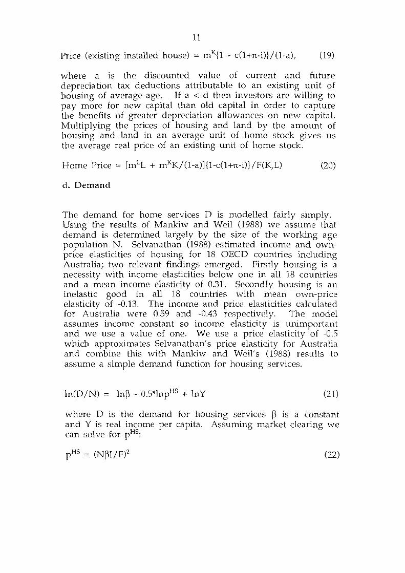
Price (existing installed house)= mK{1 - c(l+rr-i)}/(1-a), (19)

where a is the discounted value of current and future depreciation tax deductions attributable to an existing unit of housing of average age. If a < d then investors are willing to pay more for new capital than old capital in order to capture the benefits of greater depreciation allowances on new capital. Multiplying the prices of housing and land by the amount of housing and land in an average unit of home stock gives us the average real price of an existing unit of horne stock.

Horne Price = [mLL + rnKK/ (1-a)]{1-c(l +rr-i)} /F(K,L) (20)

d. Demand

The demand for horne services D is modelled fairly simply. Using the results of Mankiw and Weil (1988) we assume that demand is determined largely by the size of the working age population N. Selvanathan (1988) estimated income and own­price elasticities of housing for 18 OECD countries including Australia; two relevant findings emerged. Firstly housing is a necessity with income elasticities below one in all 18 countries and a mean income elasticity of 0.31. Secondly housing is an inelastic good in all 18 countries with mean own-price elasticity of -0.13. The income and price elasticities calculated for Australia were 0.59 and -0.43 respectively. The model assumes income constant so income elasticity is unimportant and we use a value of one. We use a price elasticity of -0.5 which approximates Selvanathan's price elasticity for Australia and combine this with Mankiw and Weil' s (1988) results to assume a simple demand function for housing services.

ln(D/N) = ln~ - O.S*lnpHS + lnY (21)

where D is the demand for housing services f3 is a constant and Y is real income per capita. Assuming market clearing we can solve for pH5:

(22)

12

3. NUMERICAL SOLUTION OF THE MODEL

In this section we specify the complete model and discuss how we simulate the model using numerical techniques for solving models containing rational expectations. We also discuss the calibration of the model at a steady state. The complete model is specified in Table 1. It is an annual model.

One problem which arises from the specification of this model is that the arbitrage conditions for land and housing prices involve expected variables. For convenience, we assume agents forn1 these expectations rationally which implies that all available information is used efficiently in forecasting future variables. Because we also assume no uncertainty, we have to find a solution where the actual evolution of variables is equal to the expected values of these variables. To solve this we use the technique developed by Fair and Taylor (1983). This algorithm involves iterating on choices for future paths of expected variables until the expected path corresponds to the actual pa th.3

To calibrate the model, '\ve can find an analytical solution for the steady state of the model. Given the pararneters such as tax rates, depreciation rates, price elasticity of housing demand, and profit share to house and land from a home package, we can solve for data that is consistent with a steady state of the model.4 Given the analytical solution for the steady state, we can calculate the values of all other variables. The values of each variable in the initial steady-state and the initial parameter assumptions are contained in Table 2.

3The algorithm used is FAIRT AYLOR which 1s written in GAUSS and available from Aptech Systems.

4 Details are provided in Appendix IV.

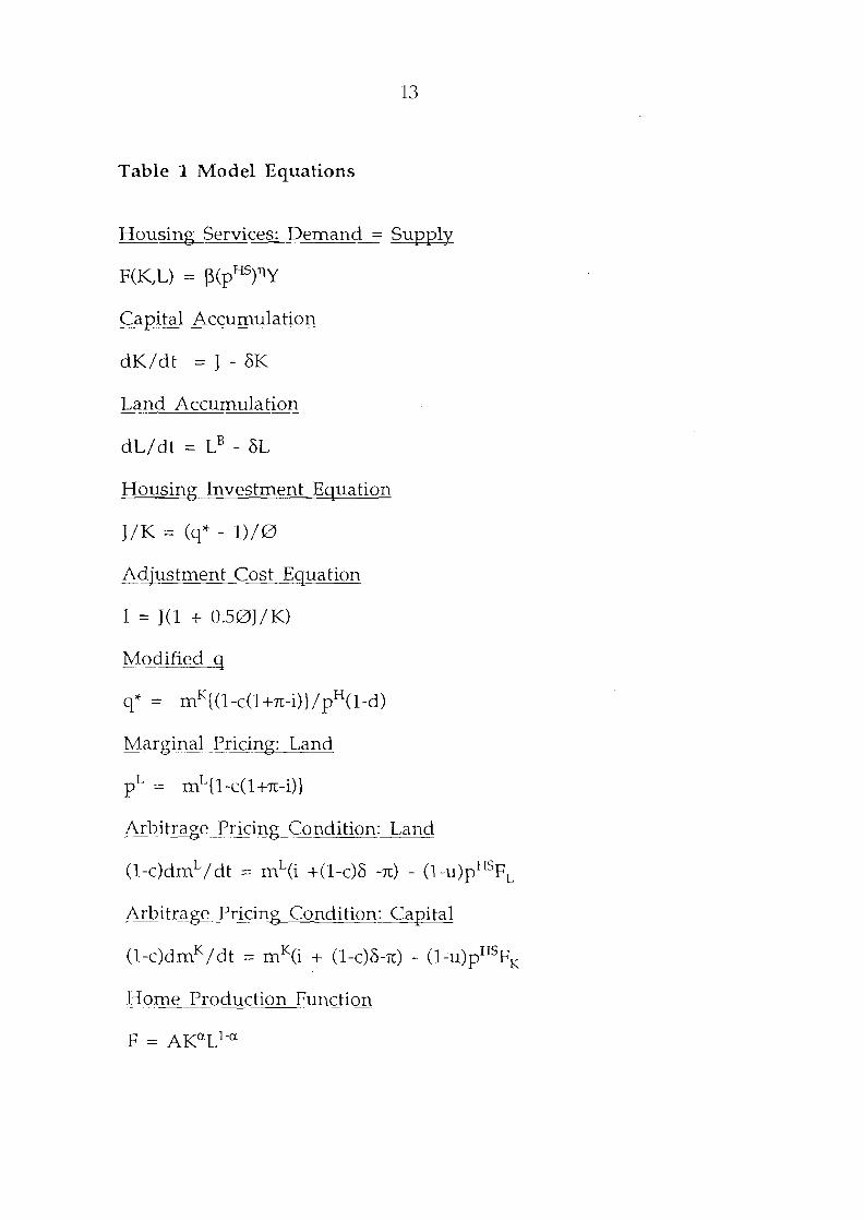
13

Table 1 Model Equations

Housing Services: Demand == Supply

F(K,L) = ~(pH5) 11Y

Capital Accumulation

dK/dt == J - 8K

Land Accumulation

dL/dt = L8- 8L

Housing Investment Equation

J/K = (q* - 1)/0

Adjustment Cost Equation

I = J(l + 0.50J/K)

11odified q

q* = mK[ (1-c(1 +n:-i)} I pH(l-d)

Margi11al Pricing: Land

pL ::.:: mL(1-c(1+n:-i)}

Arbitrage Pricing Condition: Land

(1-c)dmL/dt =:: ll1L(i +(1-c)8 -n:) - (1-u)pHSpL

Arbitrage Pricing Condition: Capital

(1-c)dmK/dt == mK(i + (1-c)8-rc) - (1-u)pH5FK

Home Production Function

F = AKet.Ll-et.

14

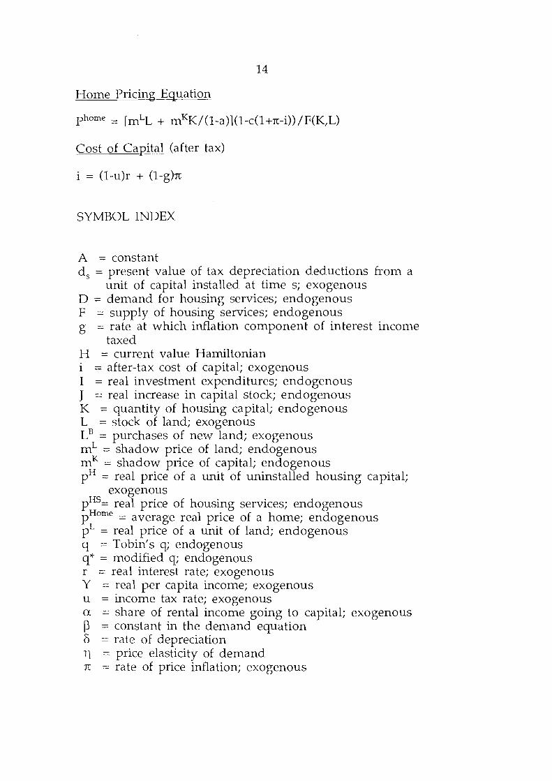
Home Pricing Equation

phome = [mLL + mKK/(1-a)](l-c(l +n:-i)) /F(K,L)

Cost of Capital (after tax)

i = (1-u)r + (1-g)n:

SYMBOL INDEX

A = constant d

5 = present value of tax depreciation deductions from a

unit of capital installed at time s; exogenous D = demand for housing services; endogenous F = supply of housing services; endogenous g = rate at which inflation component of interest income

taxed H = current value Hamiltonian i = after-tax cost of capital; exogenous I = real investment expenditures; endogenous J = real increase in capital stock; endogenous K = quantity of housing capital; endogenous L = stock of land; exogenous LB = purchases of new land; exogenous mL = shadow price of land; endogenous mK = shadow price of capital; endogenous pH = real price of a unit of uninstalled housing capital;

exogenous pH5= real price of housing services; endogenous pHome = average real price of a home; endogenous pL = real price of a unit of land; endogenous q == Tobin's q; endogenous q* = modified q; endogenous r = real interest rate; exogenous Y = real per capita income; exogenous u = income tax rate; exogenous a = share of rental income going to capital; exogenous ~ = constant in the demand equation 8 = rate of depreciation 11 = price elasticity of demand rr = rate of price inflation; exogenous

15

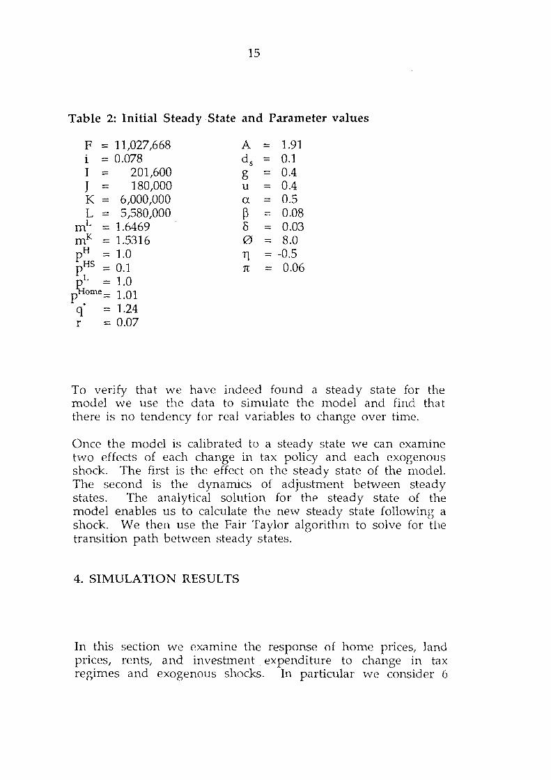
Table 2: Initial Steady State and Parameter values

F = 11,027,668 A = 1.91 1 = 0.078 ds = 0.1 I = 201,600 g = 0.4 J = 180,000 u = 0.4 K = 6,000,000 a = 0.5 L = 5,580,000 ~ = 0.08

mL = 1.6469 8 = 0.03 mK = 1.5316 0 = 8.0 PH = 1.0 11 = -0.5 PHS = 0.1 n = 0.06

L = 1.0 p~ome= 1.01

q = 1.24 r = 0.07

To verify that we have indeed found a steady state for the model we use the data to simulate the model and find that there is no tendency for real variables to change over tim.e.

Once the model is calibrated to a steady state we can examine two effects of each change in tax policy and each exogenous shock. The first is the effect on the steady state of the model. The second is the dynamics of adjustment between steady states. The analytical solution for the steady state of the model enables us to calculate the new steady state following a shock. We then use the Fair Taylor algorithm to solve for the transition path between steady states.

4. SIMULATION RESULTS

In this section we examine the response of home prices, land prices, rents, and investment expenditure to change in tax regimes and exogenous shocks. In particular we consider 6

16

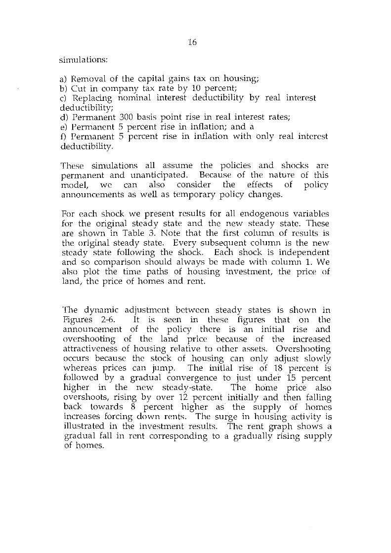
simulations:

a) Removal of the capital gains tax on housing; b) Cut in company tax rate by 10 percent; c) Replacing nominal interest deductibility by real interest deductibility; d) Permanent 300 basis point rise in real interest rates; e) Permanent 5 percent rise in inflation; and a f) Permanent 5 percent rise in inflation with only real interest deductibility.

These simulations all assume the policies and shocks are permanent and unanticipated. Because of the nature of this model, we can also consider the effects of policy announcements as well as temporary policy changes.

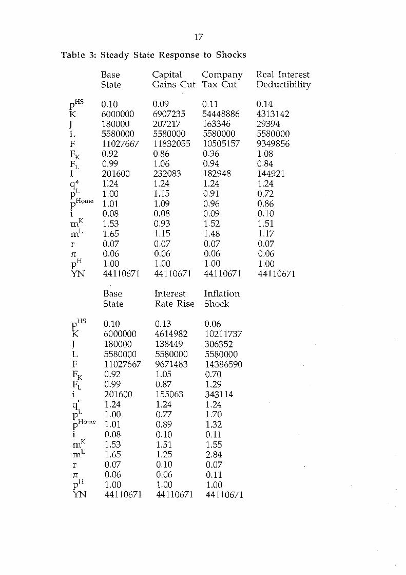
For each shock we present results for all endogenous variables for the original steady state and the new steady state. These are shown in Table 3. Note that the first column of results is the original steady state. Every subsequent column is the new steady state following the shock. Each shock is independent and so comparison should always be made with column 1. We also plot the time paths of housing investment, the price of land, the price of homes and rent.

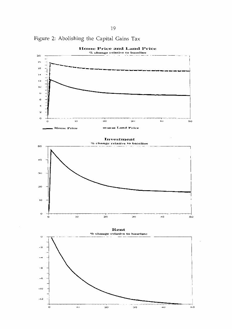
The dynamic adjustment between steady states is shown in Figures 2-6. It is seen in these figures that on the announcement of the policy there is an initial rise and overshooting of the land price because of the increased attractiveness of housing relative to other assets. Overshooting occurs because the stock of housing can only adjust slowly whereas prices can jump. The initial rise of 18 percent is followed by a gradual convergence to just under 15 percent higher in the new steady-state. The home price also overshoots, rising by over 12 percent initially and then falling back towards 8 percent higher as the supply of homes increases forcing down rents. The surge in housing activity is illustrated in the investment results. The rent graph shows a gradual fall in rent corresponding to a gradually rising supply of homes.

17

Table 3: Steady State Response to Shocks

Base Capital Company Real Interest State Gains Cut Tax Cut Deductibility

PHS 0.10 0.09 0.11 0.14 K 6000000 6907235 54448886 4313142 J 180000 207217 163346 29394 L 5580000 5580000 5580000 5580000 F 11027667 11832055 10505157 9349856 FK 0.92 0.86 0.96 1.08 FL 0.99 1.06 0.94 0.84 I 201600 232083 182948 144921 q* 1.24 1.24 1.24 1.24 PL 1.00 1.15 0.91 0.72 pH orne 1.01 1.09 0.96 0.86 1 0.08 0.08 0.09 0.10 mK 1.53 0.93 1.52 1.51 mL 1.65 1.15 1.48 1.17 r 0.07 0.07 0.07 0.07 rc 0.06 0.06 0.06 0.06 PH 1.00 1.00 1.00 1.00 YN 44110671 44110671 44110671 44110671

Base Interest Inflation State Rate Rise Shock

PHS 0.10 0.13 0.06 K 6000000 4614982 10211737 J 180000 138449 306352 L 5580000 5580000 5580000 F 11027667 9671483 14386590 FK 0.92 1.05 0.70 FL 0.99 0.87 1.29 1 201600 155063 343114 . 1.24 1.24 1.24 qL p 1.00 0.77 1.70 pH orne 1.01 0.89 1.32 1 0.08 0.10 0.11 mK 1.53 1.51 1.55 mL 1.65 1.25 2.84 r 0.07 0.10 0.07 rc 0.06 0.06 0.11 PH 1.00 1.00 1.00 YN 44110671 44110671 44110671

18

a. Removal of Capital Gains Tax on Housing

In this simulation we assume the capital gains tax is reduced from 30 percent to zero in period 1. The consequences of this for the steady state is shown in column 2 of Table 3. The new steady state has a larger stock of houses which implies a larger stock of homes, higher home prices and land prices and lower rent.

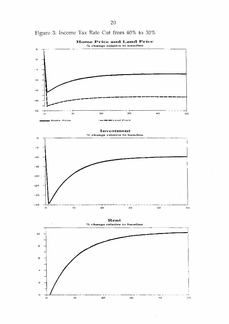
b. Cut in company tax rate by 10 percent

In the second simulation we assume that the marginal tax rate on the income of housing investors falls from 40 percent to 30 percent. The new steady state resulting from this shock is shown in column 3 of Table 1. Recall that inflation is set at six per cent per annum. Lowering tax decreases the size of the inflation tax distortion and therefore decreases the housing subsidy. In this case we get the opposite to the removal of the capital gains tax. Land prices, home prices and investment fall initially but then rise over time to a new steady state with lower prices, higher rent and a smaller housing stock. When the marginal tax rate falls housing as a form of investment becomes relatively less attractive because the taxation advantages of housing become less important.

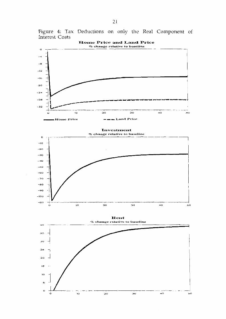
c. Replacing nominal interest deductibility by real interest deductibility

Inflation is important in this model because nominal interest payments are deductible for housing investors. In this section we simulate the removal of this policy and its replacment by real interest deductability. We see from column 4 of Table 3 that the effect of this policy on the new steady state is to reduce the housing stock and with it the price of homes and land. Rent on the other hand rises in the new steady state reflecting the fall in rental accomodation.

In Figure 4 we again see an overshooting of prices in response to the shock. Home prices intially fall by over 25 percent before rising back to 16 percent below the previous level. Investment is also severely hit by the policy. Rent rises gradually over time as the existing stock of homes falls. Note

19

Figure 2: Abolishing the Capital Gains Tax

20

IFJ

16

... 12

10

B

6

.. 2

0

~ j

0 10

Home Price and Land Price % change relative to baseline

20 30

_..... Home Price --- Lund Price

Investment % change relative to baseline

so

.. a

30

20

10

0

0 10 20 30

Rent o/o change relat:ive to b·aseline

0

-2

-6

-8

-10

-12

0 10 20 30

J .. a so

.. a so

.. a so

20

Figure 3: Income Tax Rate Cut from 40% to 30%

0

-2

-10

-12

0

-Hom-e- Pc-lc-e-

0

-s

-10

-1.5

-2o-

-25

-30

-35

0

10

B

6

2

0

0

10

10

Home Price and Land Price o/o change relat:ive t:o baseline

20 30

·---L•nd P.-llce

Investment: o/o change relat:ive t:o baseline

Rent: o/o change relat:ive t:o baseline

20 30

... a 60

-<0 so

21

Figure 4: Tax Deductions on only the Real Component of Interest Costs

0

-16

-;20

-28

-Home Price

0

-10

-20

-30

_ .. 0

-so

-60

-70

-80

-90

-100

-110 0

.. a

35

30

2.5

:zo

15

10

5

0 0

Home Price and Land Price o/c change relative t:o baseline

--- Land Price

Invest:n:1ent: o/o change relative t:o baseline

Rent: o/o change rela'tive 'to baseline

22

that the effect of this policy is more pronounced than simply lowering tax rates.

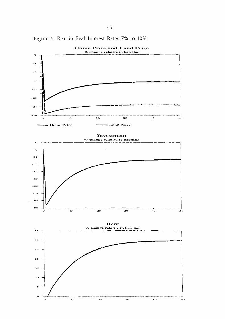
d. Permanent 300 basis point rise in real interest rates

In this simulation we assume that real interest rates rise permanently by 300 basis points. The result is quite intuitive. The new steady state shown in column 6 of Table 3 has a lower stock of homes as investors substitute away from housing into other assets. In Figure 5 we show the dynamics of adjustment. Note that home prices initially fall by 20 percent before gradually rising to around 13 percent below their intial level.

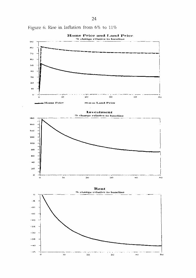
e. Permanent 5 percent rise in inflation

The results for a rise in inflation are given in column 7 of Table 3 and Figure 6. The steady-state consequences of the shock are noticably different to the real interest rate shock. In the case of the inflation shock, the distortion caused by the tax system leads to increased demand for investment housing which drives up the price of land and homes and drives rent down as the new stock of homes is constructed.

The interesting comparison between this shock and the real mterst rate shock is that both lead to a rise in nominal interest rates. So we have a result where a rise in nominal interest rates leads to a fall in investment and a case where the same rise could lead to a rise in housing investment. The important distinction is whether the change in nominal interest rates reflects expected inflation, or a rise in real rates.

f. Permanent 5 percent rise in inflation with only real interest deductibility

The results for an inflation shock without nmninal deductability are not shown because nothing happens to any real variables. All nominal variables change by the rate of inflation.

23

Figure 5: Rise m Real Interest Rates 7% to 10%

0

-~

-a

-12

-16

-20

-2~

-28 0 10

-- IIon~e Price

0

-10

-20

-30

-~0

-so

-60

-70

-80

-90

0 10

35

r 30

:zs

20

lS

10

l 5 J

I 0 i

0 10

Home Price and Land Price o/o change relative to baseline

20 30

--- Land Price

Investment 0 /o claange relative t:o baselin.e

20 30

Rent o/o clauu.ge relative t:o baselU.e

::20 30

.. a 50

~a so

~0 so

24

Figure 6: Rise 1n Inflation frmn 6% to 11%

90

BO

70

60

... 0

3o

20

IO

0

0

~Home

lBO

160

l ... o

1:20

100

BO

60

.. a

20

0

0

0

-5

-10

-IS

-20

-25

-30

-35

- ... o

- .. s 0

10

Price

10

lO

Home Price and Land Price o/o change rela~ive to baseline

20 30

----Land Price

Invest:ment: o/o Change relative to baseline

;20 30

Rent: o/o change relative to baseline

20 30

.. o 50

.. o 50

-10 so

25

5. CONCLUSION

In this paper we have constructed a simulation model of the Australian housing market which we argue incorporates many of the important features of housing. The use of an intertemporal framework allows us to examine the relationship between house pricesr land prices, rental return on housing and the evolution of the stock of homes. We then use the model to examine the consequences of changes to tax policy and shocks which are exogenous to the model such as changes in real interest rates and changes in the underlying rate of goods price inflation.

Several interesting results en1erge from this study. One result which is worth highlighting 1s the different relationship between a nse in nominal interest rates and housing investment. We showed that a rise in interest rates that reflected a change in real interest rates reduced the housing stock but a rise in nominal interest rates that reflected a rise in inflation with no change in real interest rates actually increased real investment in housing due to the tax distortions in the modeL

Econornists have been interested in the static effects of tax distortions for some time. Unfortunately tax distortions that affect the allocation of goods and production over time have received less analysis. This has been due to the difficulty of performing the analysis. Simulation models such as the one described in this paper are one way of performing analysis on intertemporal tax issues. Although the analysis is more abstract and perhaps less intuitive than shifting supply and demand curvesr the magnitude of distortions suggested by our analysis indicates that research in this area is warranted.

We found that tax policy has a large effect on the housing market as we model it. Our most interesting result was that economy-wide inflation has an important impact on the housing market due to interactions of nominal and real magnitudes with current tax arrangements in Australia. One key result is that a change to the income tax rate of housing investors has a much smaller effect on the housing market than replacing the deductibility of nominal interest payments

26

by real interest payment deductibility. Another is that for investment to remain constant real interest rates have to rise as inflation rises. This may help us explain why in Australia (a country with relatively high inflation) real interest rates are considerably higher than in countries with lower rates of inflation.

There are a variety of natural extensions of the basic n1odel that we have developed including introducing population growth. We leave these for future research.

27

APPENDIX I

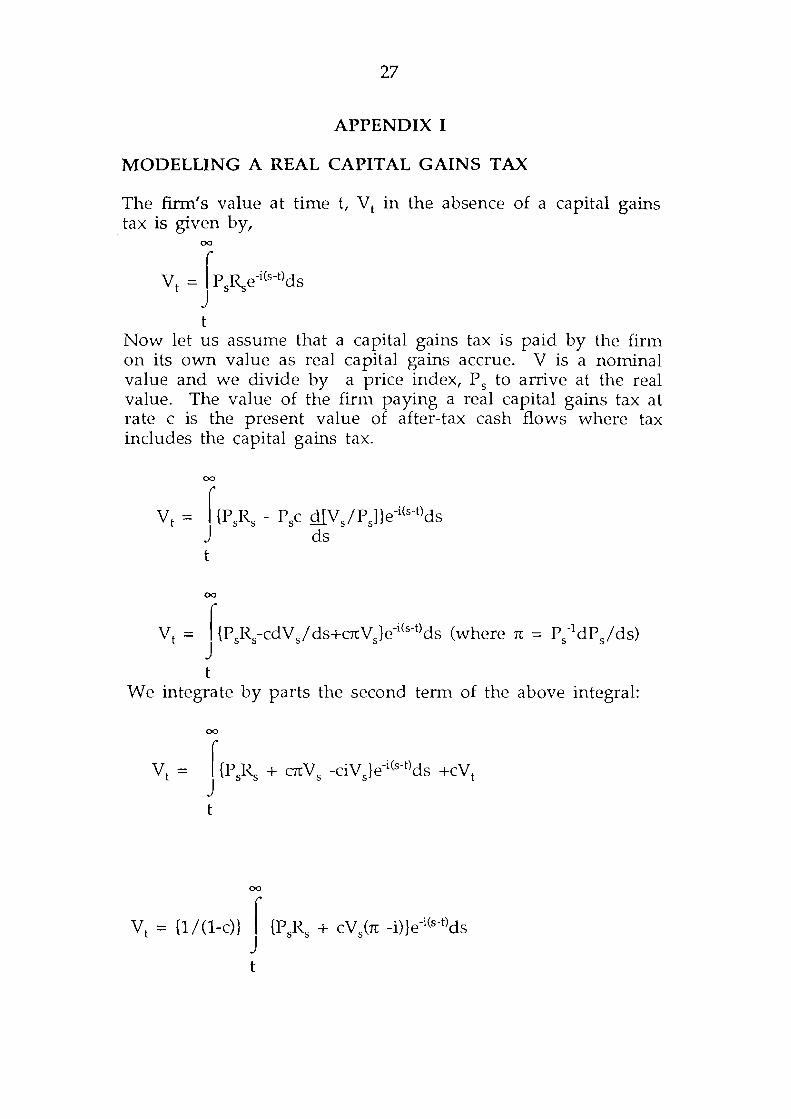
MODELLING A REAL CAPITAL GAINS TAX

The firm's value at time t, Vt in the absence of a capital gains tax is given by,

00

V = ~ p R e-i(s-t)ds t j s.._'s

t Now let us assume that a capital gains tax is paid by the firm on its own value as real capital gains accrue. V is a nominal value and we divide by a price index, P 5 to arrive at the real value. The value of the finn paying a real capital gains tax at rate c is the present value of after-tax cash flows where tax includes the capital gains tax.

00

Vt = JJ{PsRs - P5c g_[VJPs]}e-ics-t>ds ds

t

00

I {P5R

5-cdVJ ds+rnVJe-iCs-t)ds (where n = P

5-1dP

5/ ds)

J t

We integrate by parts the second term of the above integral:

00

I{P R + rnV -ciV }e-i(s-t)ds +cV j s.._'s s s t

t

00

28

APPENDIX II

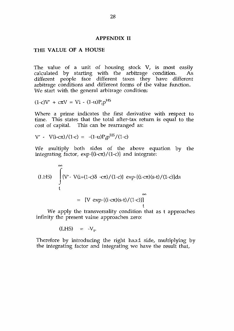
THE VALUE OF A HOUSE

The value of a unit of housing stock V, is most easily calculated by starting with the arbitrage condition. As different people face different taxes they have different arbitrage conditions and different forms of the value function. We start with the general arbitrage condition:

(1-c)V' + crrV = Vi - (1-u)PtpHS

Where a prime indicates the first derivative with respect to time. This states that the total after-tax return is equal to the cost of capital. This can be rearranged as:

V' - V(i-cn:)l(1-c) = -(1-u)PtpHS 1(1-c)

We multiply both sides of the above equation by the integrating factor, exp-{(i-cn:)l(l-c)} and integrate:

(LHS)

00

r {V'- V(i+(1-c)8 -en:) I (1-c)} exp-{(i-cn:)(s-t) I (1-c)}ds J t

00

= [V exp-{ (i -en:) (s-t) I (1-c)}] t

We apply the transversality condition that as t approaches infinity the present value approaches zero:

(LHS) = -V t-

Therefore by introducing the right ha...1d. side, multiplying by the integrating factor and integrating we have the result that,

29

(X)

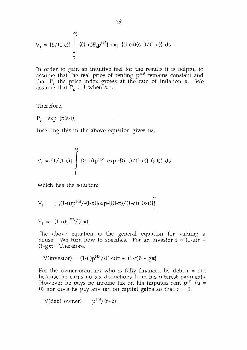
Vt = {1/(1-c)} r {(1-u)P5pHS} exp-{(i-cn;)(s-t)/(1-c)} ds

j t

In order to gain an intuitive feel for the results it is helpful to assume that the real price of renting pHS remains constant and that P

5 the price index grows at the rate of inflation n. We

assume that P5 = 1 when s=t.

Therefore,

P s =exp {n(s-t)}

Inserting this in the above equation gives us,

(X)

Vt = {1/(1-c)} r {(1-u)pHS} exp-{[(i-n)/(1'-C)) (s-t)} ds j t

which has the solution:

(X)

Vt = [ {(1-u)pHS/-(i-n)}exp-{((i-n;)/(1-c)) (s-t)}] t

The above equation is the general equation for valuing a house. We turn now to specifics. For an investor i = (1-u)r + (1-g)n. Therefore,

V(investor) = (1-u)pH5/{(1-u)r + (1-c)o- gn}

For the owner-occupant who is fully financed by debt i = r+n because he earns no tax deductions from his interest pa.rrments. However he pays no income tax on his imputed rent p 5 (u = 0) nor does he pay any tax on capital gains so that c = 0.

V(debt owner) = pHs /(r+o)

30

The happy person who owns his house outright has a discount rate i = (1-u)r + (1-g)n:. This is not because the person is negative gearing but rather because this represents the opportunity cost of investing his funds elsewhere. No capital gains tax is paid so c=O, and no tax is paid on the imputed rent (u = 0).

V(equity owner) = pHS I {(1-u)r-gn:}

Substituting numerical values into these equations it becomes apparent that the present regime is extremely biased towards equity buyers and investors. This bias is manifest in the market by the withdrawal of the first horne buyer from the property market. The first horne buyer norrnall y has to finance his purchase predominantly with debt.

31

APPENDIX III

VALUING THE DEPRECIATION ALLOWANCE

Under the present tax laws the depreciation allowance is 2.5 per cent of the cost of construction each year for forty years. The tax saving in any year is equal to the depreciation allowance multiplied by the tax rate. This saving occurs each year for forty years. The present value of this annual saving is easily calculated by discounting the cash flow savings by the cost of capital i. The value of d is given by:

d = 0.025u(l - (l+i)40)/i.

The above formula is the formula for an annuity paying 0.04u each year for forty years and is given in any finance textbook. Note that d is the present value of tax savings as a fraction of in vestrnen t expenditure.

32

APPENDIX IV

THE STEADY STATE SOLUTION

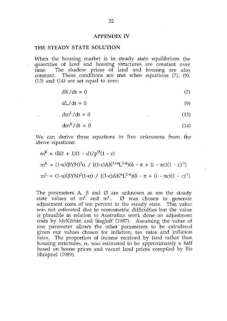
When the housing market is in steady state equilibrium the quantities of land and housing structures are constant over time. The shadow prices of land and housing are also constant. These conditions are met when equations (7), (9), (13) and (14) are set equal to zero:

dKidt = 0

dLidt = 0

dmLidt = 0

dmKidt = 0

(7)

(9)

(13)

(14)

We can derive three equations 1n five unknowns from the above equations:

mK = (80 + 1)(1 - d)lpH(l - c)

mK = (1-u)(~YN)2a I {(1-c)AK1+aL1-o.)(o - n + (i - nc)(l - ct1}

mL = (1-u)(~YN)2(1-a) I {(1-c)AKaL2-a)(o - n + (i - nc)(l - ct1}

The parameters A, ~ and 0 are unknown as are the steady state values of mk and mL. 0 was chosen to generate adjustment costs of ten percent in the steady state. This value was not esti1nated due to econometric difficulties but the value is plausible in relation to Australian work done on adjustment costs by McKibbin and Siegloff (1987). Assuming the value of one parameter allows the other parameters to be calculated given our values chosen for inflation, tax rates and inflation rates. The proportion of income received by land rather than housing structures, a, was estimated to be approximately a half based on house prices and vacant land prices compiled by Bis Shrapnel (1989).

33

REFERENCES

Abel, A.B. (1982) "Dynamic Effects of Permanent and Temporary Tax Policies in a q Model of Investment", Journal of Monetary Economics, 9, 353-373.

Alban, R. (1989) "Housing and Taxation - Commonwealth Issues", National Housing Conference, Canberra March.

His-Shrapnel (1989) Building in Australia: 1989-2003.

Fair, R. and Taylor, J. (1983) "Solution and Maximum Likelihood Estimation of Dynamic Nonlinear Rational Expectations Models", Econometrica, 51, July, 1169-1185.

Hall, R.E. and Jorgenson, D.W. (1967) "Tax Policy and Investment Behaviour", American Economic Review, 57, June, 391-414.

Hayashi, F. (1982) "Tobin's Marginal q and Average q: A Neoclassical Interpretation", Econometrica, 50, January, 213-224.

Mankiw, N.G. and Weil, D.N. (1988) "The Baby Boom, the Baby Bust, and the Housing Market", Harvard Institute of Economic Research, Discussion Paper No. 1414, December.

McKibbin, W.J. and Siegloff, E.S. (1987) "A Note on Aggregate Investment in Australia" Reserve Bank of Australia, Research Discussion Paper 8709.

Nevile, J.W., Tran-Nam, B., Vipond, J. and Warren, N.A, (1987) "A Simple Model of Recent Changes in the Residential Property Market", Economic Record, 63, September, 270-280.

Selvanathan, S. (1988) "Empirical Regularities in OECD Consumption", Economic Research Centre, The University of Western Australia, Discussion Paper 88.01, March.

Tobin, J. (1969) Monetary Theory", February, 15-29.

"A General Equilibrium Approach to Journal of Money, Credit and Banking, 1,