tax capacity and growth: is there a tipping point? - imf · tax capacity and growth: is there a...

WP/16/234

Tax Capacity and Growth: Is there a Tipping Point?

by Vitor Gaspar, Laura Jaramillo and Philippe Wingender

IMF Working Papers describe research in progress by the author(s) and are published

to elicit comments and to encourage debate. The views expressed in IMF Working Papers

are those of the author(s) and do not necessarily represent the views of the IMF, its

Executive Board, or IMF management.

2

© 2016 International Monetary Fund WP/16/234

IMF Working Paper

Fiscal Affairs Department

Tax Capacity and Growth: Is there a Tipping Point?

Prepared by Vitor Gaspar, Laura Jaramillo and Philippe Wingender1

Authorized for distribution by Vitor Gaspar

November 2016

Abstract

Is there a minimum tax to GDP ratio associated with a significant acceleration in the

process of growth and development? We give an empirical answer to this question by

investigating the existence of a tipping point in tax-to-GDP levels. We use two separate

databases: a novel contemporary database covering 139 countries from 1965 to 2011 and

a historical database for 30 advanced economies from 1800 to 1980. We find that the

answer to the question is yes. Estimated tipping points are similar at about 12¾ percent of

GDP. For the contemporary dataset we find that a country just above the threshold will

have GDP per capita 7.5 percent larger, after 10 years. The effect is tightly estimated and

economically large.

JEL Classification Numbers: H11, H26, O10, O43

Keywords: income per capita, taxation, development, multiple equilibria

Authors’ e-mail addresses: [email protected], [email protected], [email protected]

1 We are grateful to David Lipton for inspiring the research question. We thank Sanjeev Gupta, Mick Keen, Abdel

Senhadji, Bernardin Akitoby, Rossen Rozenov, Andrew Hodge, Marialuz Moreno Badia, Xavier Debrun, Vikram

Haksar, Albert Touna Mama and Aart Kraay for helpful comments and discussion. We are also grateful to

participants of the IMF Fiscal Affairs Department seminar for their useful suggestions. We thank Elijah Kimani for

excellent research assistance.

IMF Working Papers describe research in progress by the author(s) and are published to elicit

comments and to encourage debate. The views expressed in IMF Working Papers are those of the

author(s) and do not necessarily represent the views of the IMF, its Executive Board, or IMF

management.

mailto:[email protected]



3

Abstract ___________________________________________________________________________________________ 2

I. Introduction _____________________________________________________________________________________ 5

II. Taxation and economic development __________________________________________________________ 6

A. How is taxation linked to greater economic development? ____________________________________ 6

B. Tipping points: how can a small change in taxes lead to large changes in GDP? _______________ 9

C. Stylized Facts __________________________________________________________________________________ 10

III. Data __________________________________________________________________________________________ 12

IV. Empirical approach ___________________________________________________________________________ 15

A. Methodology _________________________________________________________________________________ 15

B. Results based on the contemporary database _________________________________________________ 18

C. Results based on the historical database ______________________________________________________ 25

V. Conclusion ____________________________________________________________________________________ 29

References _______________________________________________________________________________________ 31

Figures

1. Complementarities in State Capacity ___________________________________________________________ 8

2. Tax Capacity, Social Norms, and Accountability ________________________________________________ 9

3. Tax to GDP and Income Levels ________________________________________________________________ 11

4. Tax Capacity and Legal Capacity, 2012 ________________________________________________________ 11

5. Tax Capacity and Public Administration Capacity, 2012 _______________________________________ 12

6. Contemporary Database: Number of Observations for Tax to GDP ____________________________ 13

7. Contemporary Database: Distribution of Average Annual Real GDP per Capita Growth

and Tax to GDP Ratios ________________________________________________________________________ 14

8. Historical Database: Number of Observations for Tax-to-GDP ________________________________ 14

9. Historical Database: Distribution of Average Annual Real GDP per Capita Growth and

Tax to GDP _____________________________________________________________________________________ 15

10. Searching for a Tax Tipping Point at Different Horizons ______________________________________ 19

11. Impact of the Tax Threshold on 10-year Cumulative Growth _________________________________ 21

12. Impact of the Tax Threshold over Time ______________________________________________________ 23

13. Searching for a Tax Tipping Point at Different Horizons, Historical Database ________________ 26

14. Impact of the Tax Threshold on 10-year Cumulative Growth, Historical Database ____________ 27

15. Impact of the Revenue Threshold over Time, Historical Database ____________________________ 28

Tables

1. Sources for Tax-to-GDP data __________________________________________________________________ 13

2. Testing for Statistical Significance of Tax Thresholds __________________________________________ 20

3. Estimated Tax-to-GDP Thresholds _____________________________________________________________ 20

4. Estimating Growth Effects _____________________________________________________________________ 24

5. Estimating Tax Revenue-to-GDP Thresholds, Historical Database _____________________________ 27

4

6. Estimating Growth Effects, Historical Database ________________________________________________ 29

Appendix ________________________________________________________________________________________35

Appendix figure

A1. Impact of a Tax Threshold on 3-year Cumulative Growth ____________________________________ 35



Appendix tables

A1. Tipping Point Crossing, Contemporary Database ____________________________________________ 37

A2. Summary Statistics, Historical Database _____________________________________________________ 39

A3. Tipping Point Crossing, Historical Database _________________________________________________ 40

5

I. INTRODUCTION

Is there a minimum tax-to-GDP ratio associated with a significant acceleration in the

process of growth and development? This paper proposes a new way to quantify the relation

between taxes and growth by investigating the existence of a tipping point in tax-to-GDP levels.

Tipping points can occur in environments characterized by multiple equilibria and are associated

with sharp changes occurring around some threshold.

We use a novel contemporary database covering 139 countries and spanning the period

1965-2011. We combine the approaches taken by Card, Mas and Rothstein (2008) using

regression discontinuity design methods with the threshold regression framework proposed by

Hansen (1999) to provide new estimates of tax tipping points.

Our approach provides new empirical estimates that build on earlier work by Besley and

Persson (2011, 2013, 2014a, 2014b). We go beyond the existing literature in two dimensions:

(i) we rely on a much broader database, both in coverage of countries and years; and (ii) we use a

non-linear model to flexibly estimate the reduced-form relation between tax levels and

subsequent GDP growth. Specifically, we use a regression discontinuity design model to estimate

a growth tipping point.

Our focus is on tax revenues as other sources of revenue have not been found to be closely

related to economic development. Arezki et al. (2011) and IMF (2015) illustrate that countries

that have an abundance of natural resources often show a record of relatively poor economic

performance compared with non-resource-rich countries. In the case of foreign aid, there is no

consensus on its effects on economic development. Some argue that official assistance has

harmed poor countries throughout the years, while others believe that aid levels have been too

low. Edwards (2014) provides a useful overview.

From a conceptual viewpoint we follow the path openned by Joseph Schumpeter in his

famous paper The Crisis of the Tax State (Schumpeter, 1918). Schumpeter links state and tax

so closely that he stresses that his expression “tax state” can be regarded as almost pleonastic.

He emphasizes that taxes are not only associated with the historical origin of the state, they are

also active in shaping it. In his view the organic development of taxation was associated with the

organic development of other dimensions of the state. It is particularly important for our

purposes to stress Schumpeter’s distinction between taxes and other forms of government

revenue. From the viewpoint of the Tax State, the dependence on revenues from patrimony or

entrepreneurial activity is characteristic of an earlier stage of Public Finance development. For

Schumpeter, the analysis of the consequences of taxation requires a long run perspective that

allows for structural and self-reinforcing evolutionary dynamics to play out in full. These

dynamics are not only economic but also social and political. We interpret Besley and Persson as

bringing a similar perspective to contemporary research. We would like to place our contribution

within this tradition.

6

The answer to the question with which we begin the paper is made difficult by the joint

determination of GDP and the tax-to-GDP ratio. We want to investigate how tax-to-GDP is

associated with subsequent growth. But it is also the case that GDP growth is associated with

increases in the tax-to-GDP ratio. This may be rationalized, for example, in terms of the so-called

Wagner’s Law. In the process of economic development, the demand for public services

increases faster than GDP, leading to an increased in government’s expenditure-to-GDP ratio.

Since these tend to be financed, at the margin, by taxation, a similar increase in the tax-to-GDP

ratio ensues. We mitigate the issue by focusing on local effects, i.e. how small changes in taxes

around a specific tipping point lead to potentially large change in subsequent growth, as

opposed to estimating global relations such linear models. We also find that our local results are

robust when controlling for the potential endogeneity of taxes.2

The paper is organized as follows. Section II provides a short selective review on the relevant

literature on the relationship between taxation and economic development. It also discusses the

intuition on how a small change in taxes can lead to large changes in GDP. Section III describes

how we compiled our two databases—the contemporary database and the historical database.

Section IV explains the methodology used and the empirical results obtained. Section V

concludes.

II. TAXATION AND ECONOMIC DEVELOPMENT

A. How is taxation linked to greater economic development?

When studying the relationship between taxation and economic development, there is a

strand of literature that focuses on how development influences the evolution of the tax

system. The emphasis is on the economic constraints that influence the government’s ability to

impose a particular tax rate on a particular tax base. For example, Tanzi (1992) and Burgess and

Stern (1993) find that countries with a higher share of agriculture and a lower share of imports-

to-GDP tend to have lower taxation. Gordon and Li (2009) emphasize the link between taxation

and formal finance. They argue that firms have incentives to evade taxes by conducting all

business in cash in countries where the value from using the financial sector is more modest. In

the same vein, Kleven, Kreiner, and Saez (2009) show that in more developed countries, firm size

is sufficiently large to make third-party tax enforcement effective, as income witholding facilitates

cross-checking of tax records between indviduals and firms. Others have argued that large

informal sectors in poor economies are inherently hard to tax, as discussed in the survey by Joshi

et al. (2014). La Porta and Shleifer (2014) discuss the desire to avoid taxes as an important motive

for informality.

Access to forms of revenue other than taxes has also been associated with lower taxation.

Jensen (2011) finds that a 1 percent increase in the share of natural resource rents in total

government income is associated with a 1.4 percent lower share of taxation in GDP. Benedek et

al. (2014) find a negative association between foreign aid and domestic tax revenues, particularly

in low-income countries and in countries with relatively weak institutions.

2 We use the IV threshold model proposed by Caner and Hansen (2004). Results are available upon request.

7

Of course, there is another strand of literature that studies the influence of the tax system

on the economy. Barro (1990) discusses how the economy can be made more productive when

tax revenues are spent on public goods and investments. Barro and Sala-i-Martin (1992) show

that, in endogenous-growth models, well-designed tax systems can minimize the efficiency

losses imposed by taxes and can even raise the GDP growth rate. For sub-Saharan Africa, Ebeke

and Ehrhart (2011) find that the instability of tax revenue leads to the instability in public

investment and government consumption, and it also reduces the level of public investment.

Seidel and Thum (2015) argue that stricter tax enforcement forces corrupt officials to reduce

bribe demands, which makes market entry by private firms more attractive.

Several authors have augmented the standard approach, giving political and institutional

factors a key role in the analysis of taxation and development. Most notably, Besley and

Persson (2011, 2013, 2014a, 2014b) emphasize the broader concept of state capacity to stand for

a range of capabilities that are needed for the state to function effectively. State capacity

incorporates investment by the government in building three key dimensions: (i) fiscal capacity,

by increasing collection of taxes, especially broad-based taxes, through stronger tax

enforcement; (ii) legal capacity, which refers to market-supporting regulation, enforcement of

contracts, and protection of property rights; and (iii) collective capacity by augmenting markets,

mostly by supplying public goods. Besley and Persson (2011) also suggest that many

determinants of state capacity are common across these dimensions. They carry out simple

regression analyses for a cross-section of 111 countries to show the correlation between

common factors (war, ethnic homogeneity, political stability, constraints on the executive) and

measures of fiscal and legal capacity.

Building on Besley and Persson, Figure 1 illustrates the link between taxation and greater

economic development. State capacity is shaped by the interaction between tax capacity, legal

capacity, and public administration capacity. Tax capacity not only provides a stable and elastic

source of revenue for the government to finance its activities, but a government with a larger

stake in the economy through a developed tax system also has stronger motives to play a

productive role in the economy. Public administration capacity refers to the government’s

effective and efficient use of public money.3 This directly impacts the ability of governments to

implement policy and deliver public services, which in turn influences citizens’ trust in

government. Legal capacity refers to the government’s ability to secure private property rights.

This includes legal infrastructure such as building the court system and registering property.

It is important to note that tax capacity, legal capacity, and public administration capacity

are complements. Sustained improvements in tax collection do not occur in a vacuum. Building

tax capacity requires investment in legal capacity, and vice versa. This is why we would expect

tax, legal, and public administration capacity to be positively correlated with one another. These

feedback loops can also give rise to multiple equilibria as noted for example in Besley and

Persson (2013).

3 For example, Pritchett (2000a) and IMF (2015) discuss how weaknesses in public investment management have

resulted in inadequate returns to public investment in many countries.

8

The strength of tax capacity depends crucially on social norms of compliance. Kiser and

Levi (2015) emphasize that the more a government is effective and trustworthy, the more

legitimacy it is likely to attain, and the more it will be able to elicit compliance without excessive

monitoring or punitive action. Similarly, as proposed by Levi (1988), the government can achieve

a high degree of quasi-voluntary compliance with the taxation system when citizens comply with

taxation out of a combination of strategic and normative considerations. Strategic considerations

refer to the calculation of the probability of being caught and the punishment involved.

Normative considerations refer to a sense of fairness: the citizen believes that sufficient public

goods are being provided in return for tax payments, and that others are also paying their fair

share. A variety of other authors have also argued that creating a culture of compliance is central

to raising revenue. For example, Gordon (1989) refers to individual morality, Posner (2000) to tax-

compliance norms, and Torgler (2007) to tax morale. Social norms of compliance are in turn

closely associated with a higher demand by citizens for accountable and transparent

government, as argued by Moore (2007), Brautigam et al. (2008) and Ross (2004). These

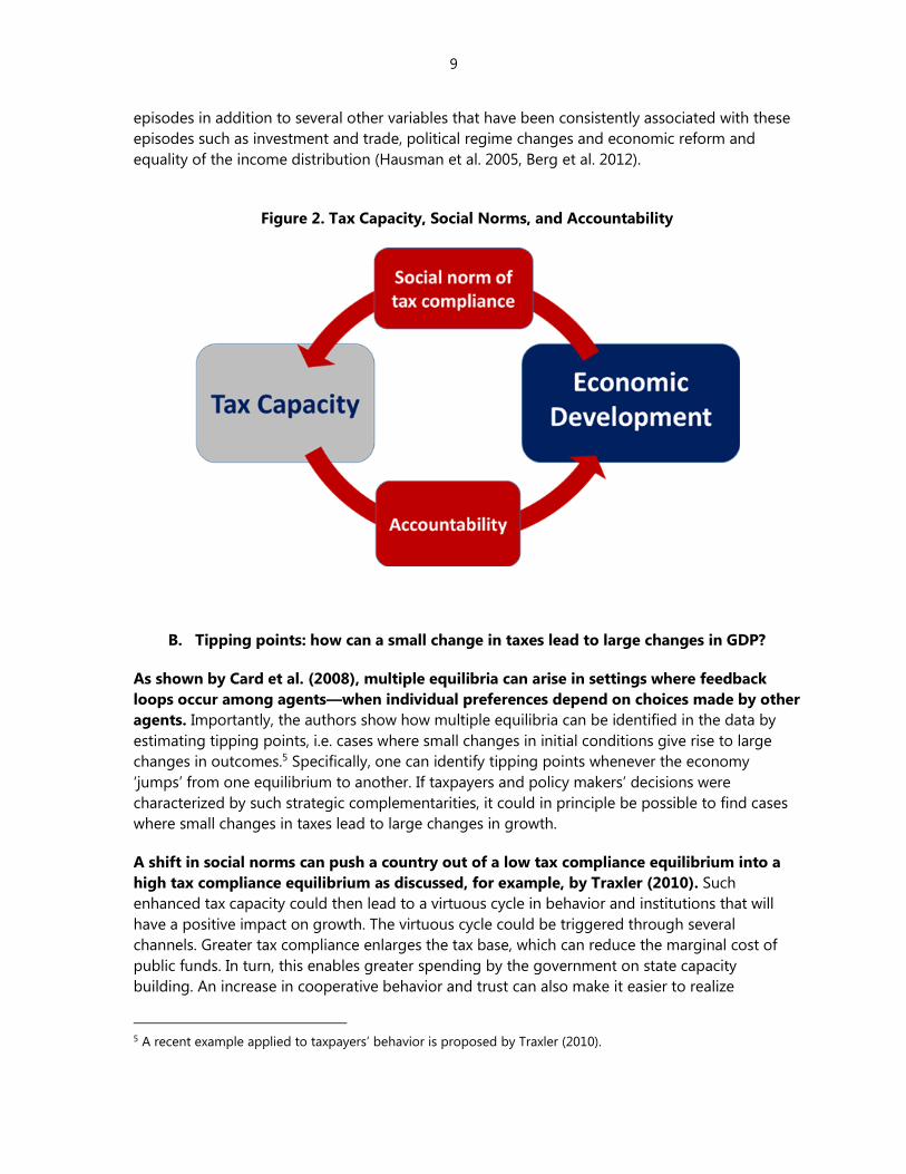
relationships are illustrated in Figure 2.

Figure 1. Complementarities in State Capacity

Finally, our paper can also be linked to the recent literature on growth accelerations (see

for example Hausman et al. 2005, Pritchett 2000b and Berg et al. 2012). While the average

effect on growth of crossing the tax-to-GDP tipping point isn't quite as high as the highest

growth acceleration episodes considered in several of these studies4, we find that average annual

growth rates are higher by about 0.75 ppa over 10 years compared to countries that remain

below the tipping point. This qualifies as an important and large driver of sustained growth

4 For example, Hausman et al. (2005) consider episode where GDP per capita growth rates increase by 2.5 ppa

sustained over 8 years.

9

episodes in addition to several other variables that have been consistently associated with these

episodes such as investment and trade, political regime changes and economic reform and

equality of the income distribution (Hausman et al. 2005, Berg et al. 2012).

Figure 2. Tax Capacity, Social Norms, and Accountability

B. Tipping points: how can a small change in taxes lead to large changes in GDP?

As shown by Card et al. (2008), multiple equilibria can arise in settings where feedback

loops occur among agents—when individual preferences depend on choices made by other

agents. Importantly, the authors show how multiple equilibria can be identified in the data by

estimating tipping points, i.e. cases where small changes in initial conditions give rise to large

changes in outcomes.5 Specifically, one can identify tipping points whenever the economy

‘jumps’ from one equilibrium to another. If taxpayers and policy makers’ decisions were

characterized by such strategic complementarities, it could in principle be possible to find cases

where small changes in taxes lead to large changes in growth.

A shift in social norms can push a country out of a low tax compliance equilibrium into a

high tax compliance equilibrium as discussed, for example, by Traxler (2010). Such

enhanced tax capacity could then lead to a virtuous cycle in behavior and institutions that will

have a positive impact on growth. The virtuous cycle could be triggered through several

channels. Greater tax compliance enlarges the tax base, which can reduce the marginal cost of

public funds. In turn, this enables greater spending by the government on state capacity

building. An increase in cooperative behavior and trust can also make it easier to realize

5 A recent example applied to taxpayers’ behavior is proposed by Traxler (2010).

10

agglomeration effects in production as more individuals and firms participate in formal markets.

Furthermore, greater accountability from a larger pool of taxpayers can improve governance and

help decrease corruption, further reducing barriers to market entry by firms and supporting

economic growth (Murphy, Schleifer, and Vishny, 1993).

We argue that as countries approach and eventually exceed some revenue threshold,

growth outcomes for these countries would then jump discontinuously. Card et al. (2008)

demonstrate that tipping points can be identified and estimated through the use of regression

discontinuity design (RDD) methods. We apply the approach to the relation between tax-to-GDP

levels and subsequent GDP growth. In particular, we look for levels of tax-to-GDP around which

we observe sharp changes in subsequent GDP growth rates. We interpret our findings as

suggestive of the possible presence of multiple equilibria in tax compliance and capacity: small

variations in tax levels around a tipping point can lead to economies jumping from one

equilibrium to another. This in turn can lead to large differences in growth as some countries

reach the high compliance/high growth equilibrium while others remain in the low

compliance/low growth equilibrium.

C. Stylized Facts

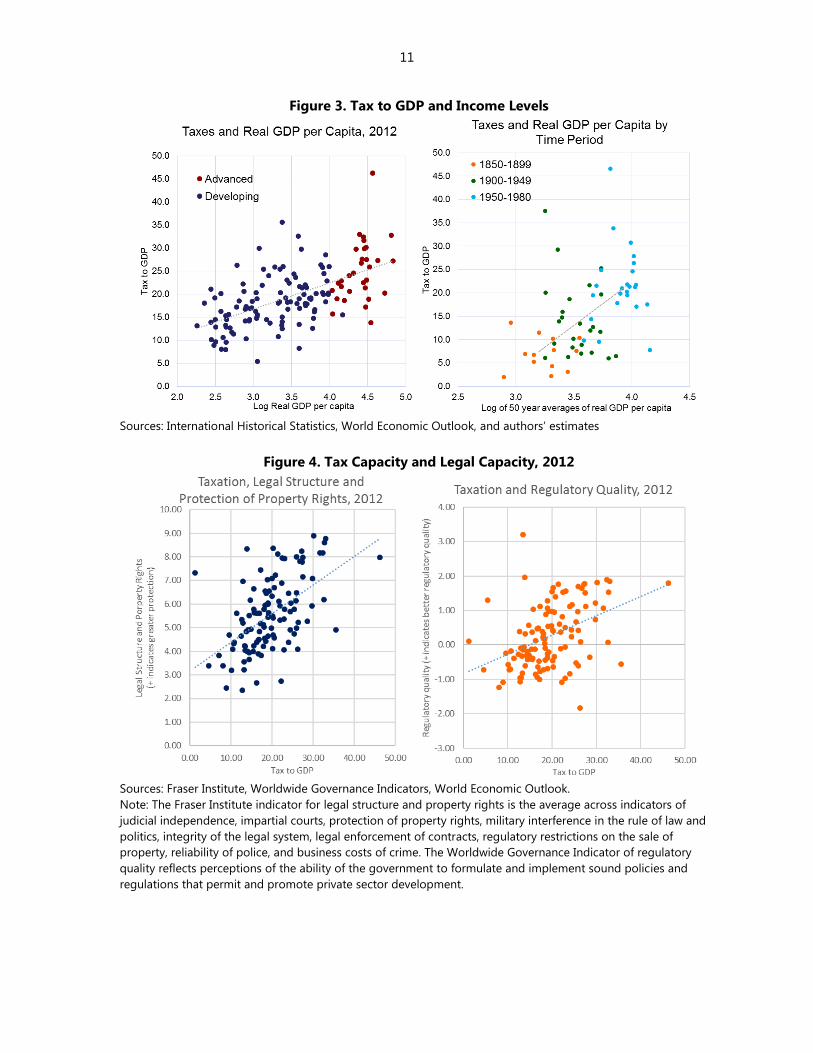
Stylized facts illustrate the relationship between tax capacity and economic development.

Figure 3 shows the positive relationship between tax-to-GDP and real GDP per capita, using two

separate samples of countries. Using a cross-section of data for 2012, the figure shows that

higher income countries tend to raise more tax revenue as a share of GDP than lower income

countries. Using historical time-series data going back to the 1800s for 30 countries, the figure

shows a similar trend, where tax-to-GDP rise over time along with income levels. These findings

are in line with the reading of Wagner’s Law that we suggested earlier.

Figure 4 illustrates the complementarity between tax capacity and legal capacity. The figure

shows that countries with higher tax revenue-to-GDP also tend to have stronger protection of

property rights, as measured by a Fraser Institute indicator of legal structure and property rights.

The figure also shows that higher tax-to-GDP is associated with higher quality of government

policies and regulation, as measured by the Worldwide Governance Indicators.

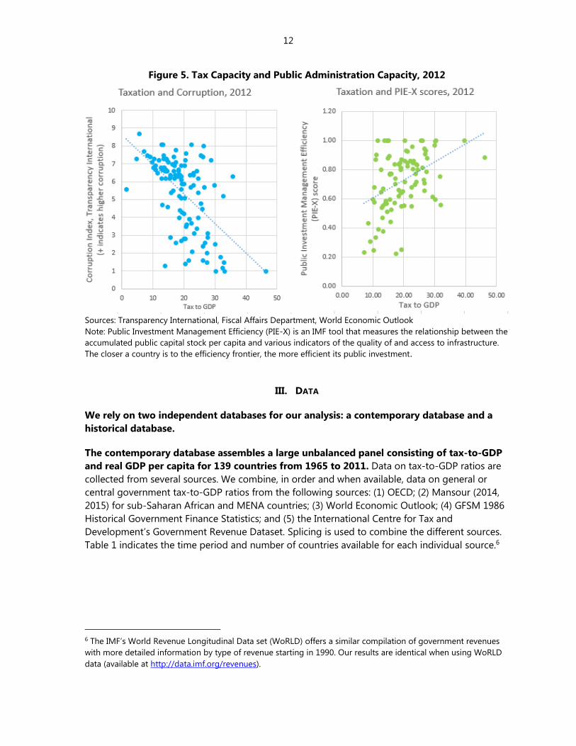
Figure 5 illustrates the complementarity between tax capacity and public administration

capacity. The figure shows a negative relationship between tax-to-GDP and a corruption index

by Transparency International. This suggests that tax capacity is once again associated with

greater government transparency and accountability. The figure also shows that countries with

higher tax-to-GDP also tend to have stronger budget institutions, as measured by the Public

Investment Management Efficiency (PIE-X) index.

11

Figure 3. Tax to GDP and Income Levels

Sources: International Historical Statistics, World Economic Outlook, and authors’ estimates

Figure 4. Tax Capacity and Legal Capacity, 2012

Sources: Fraser Institute, Worldwide Governance Indicators, World Economic Outlook.

Note: The Fraser Institute indicator for legal structure and property rights is the average across indicators of

judicial independence, impartial courts, protection of property rights, military interference in the rule of law and

politics, integrity of the legal system, legal enforcement of contracts, regulatory restrictions on the sale of

property, reliability of police, and business costs of crime. The Worldwide Governance Indicator of regulatory

quality reflects perceptions of the ability of the government to formulate and implement sound policies and

regulations that permit and promote private sector development.

12

Figure 5. Tax Capacity and Public Administration Capacity, 2012

Sources: Transparency International, Fiscal Affairs Department, World Economic Outlook

Note: Public Investment Management Efficiency (PIE-X) is an IMF tool that measures the relationship between the

accumulated public capital stock per capita and various indicators of the quality of and access to infrastructure.

The closer a country is to the efficiency frontier, the more efficient its public investment.

III. DATA

We rely on two independent databases for our analysis: a contemporary database and a

historical database.

The contemporary database assembles a large unbalanced panel consisting of tax-to-GDP

and real GDP per capita for 139 countries from 1965 to 2011. Data on tax-to-GDP ratios are

collected from several sources. We combine, in order and when available, data on general or

central government tax-to-GDP ratios from the following sources: (1) OECD; (2) Mansour (2014,

2015) for sub-Saharan African and MENA countries; (3) World Economic Outlook; (4) GFSM 1986

Historical Government Finance Statistics; and (5) the International Centre for Tax and

Development’s Government Revenue Dataset. Splicing is used to combine the different sources.

Table 1 indicates the time period and number of countries available for each individual source.6

6 The IMF’s World Revenue Longitudinal Data set (WoRLD) offers a similar compilation of government revenues

with more detailed information by type of revenue starting in 1990. Our results are identical when using WoRLD

data (available at http://data.imf.org/revenues).

http://data.imf.org/revenues

13

Table 1. Sources for Tax-to-GDP data

Database Period Countries

Tax-to-GDP (all sources) 1965-2011 139

1- OECD 1965-2011 47

2- Mansour (2014, 2015) 1980-2011 38

3- World Economic Outlook 1985-2011 77

4- GFSM 1986 Historical Government Finance Statistics 1970-2002 70

4- The International Centre for Tax and Development 1980-2010 40

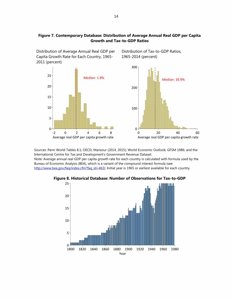
To study growth across countries and over time, we use real GDP per capita at constant

national prices, obtained the Penn World Tables 8.1 (Feenstra, Inklaar and Timmer, 2015).7

Figure 6 shows the number of observations on tax-to-GDP available by year for advanced and

developing countries. Figure 7 shows the distribution of tax-to-GDP and average annual real per

capita GDP growth rates across the contemporary database.

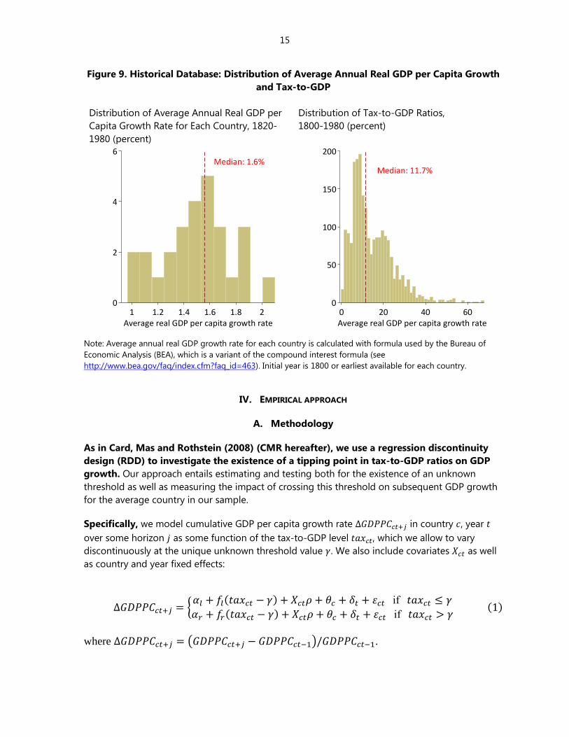
The historical database is also an unbalanced panel consisting of tax-to-GDP ratios and

real GDP per capita for 30 advanced countries between 1800 and 1980.8 Data on tax-to-GDP

is from the International Historical Statistics (Mitchell, 2003). Data on real GDP per capita (in

GK$ 1990) is from the Maddison Project 2013 version. Figure 8 shows the number of

observations on tax-to-GDP by year. Figure 9 shows the distribution of tax-to-GDP and average

annual real per capita GDP growth rates across the historical database.

Figure 6. Contemporary Database: Number of Observations for Tax to GDP

7 We drop from our sample countries where natural resource rents, as measured in the World Development

Indicators, exceeds 30 percent on average over the entire sample.

8 Countries are: Australia, Austria, Belgium, Canada, Chile, Czech Republic, Denmark, Estonia, Finland, France,

Germany, Greece, Hungary, Israel, Italy, Japan, Korea, Mexico, Netherlands, New Zealand, Norway, Poland,

Portugal, Slovenia, Ireland, Spain, Sweden, Switzerland, United Kingdom, United States.

0

50

100

150

1965 1970 1975 1980 1985 1990 1995 2000 2005 2010Year

Emerging

Advanced

14

Figure 7. Contemporary Database: Distribution of Average Annual Real GDP per Capita

Growth and Tax-to-GDP Ratios

Distribution of Average Annual Real GDP per

Capita Growth Rate for Each Country, 1965-

2011 (percent)

Distribution of Tax-to-GDP Ratios,

1965-2014 (percent)

Sources: Penn World Tables 8.1; OECD; Mansour (2014, 2015); World Economic Outlook; GFSM 1986; and the

International Centre for Tax and Development’s Government Revenue Dataset.

Note: Average annual real GDP per capita growth rate for each country is calculated with formula used by the

Bureau of Economic Analysis (BEA), which is a variant of the compound interest formula (see

http://www.bea.gov/faq/index.cfm?faq_id=463). Initial year is 1965 or earliest available for each country.

Figure 8. Historical Database: Number of Observations for Tax-to-GDP

Median: 1.9%

0

5

10

15

20

25

Nu

mb

er

of

cou

ntr

ies

-2 0 2 4 6 8Average real GDP per capita growth rate

Median: 16.9%

0

100

200

300

Nu

mb

er

of

cou

ntr

y/ye

ars

0 20 40 60Average real GDP per capita growth rate

0

5

10

15

20

25

1800 1820 1840 1860 1880 1900 1920 1940 1960 1980Year

http://www.bea.gov/faq/index.cfm?faq_id=463

15

Figure 9. Historical Database: Distribution of Average Annual Real GDP per Capita Growth

and Tax-to-GDP

Distribution of Average Annual Real GDP per

Capita Growth Rate for Each Country, 1820-

1980 (percent)

Distribution of Tax-to-GDP Ratios,

1800-1980 (percent)

Note: Average annual real GDP growth rate for each country is calculated with formula used by the Bureau of

Economic Analysis (BEA), which is a variant of the compound interest formula (see

http://www.bea.gov/faq/index.cfm?faq_id=463). Initial year is 1800 or earliest available for each country.

IV. EMPIRICAL APPROACH

A. Methodology

As in Card, Mas and Rothstein (2008) (CMR hereafter), we use a regression discontinuity

design (RDD) to investigate the existence of a tipping point in tax-to-GDP ratios on GDP

growth. Our approach entails estimating and testing both for the existence of an unknown

threshold as well as measuring the impact of crossing this threshold on subsequent GDP growth

for the average country in our sample.

Specifically, we model cumulative GDP per capita growth rate ∆𝐺𝐷𝑃𝑃𝐶𝑐𝑡+𝑗 in country 𝑐, year 𝑡

over some horizon 𝑗 as some function of the tax-to-GDP level 𝑡𝑎𝑥𝑐𝑡, which we allow to vary

discontinuously at the unique unknown threshold value 𝛾. We also include covariates 𝑋𝑐𝑡 as well

as country and year fixed effects:

∆𝐺𝐷𝑃𝑃𝐶𝑐𝑡+𝑗 = {𝛼𝑙 + 𝑓𝑙(𝑡𝑎𝑥𝑐𝑡 − 𝛾) + 𝑋𝑐𝑡𝜌 + 𝜃𝑐 + 𝛿𝑡 + 휀𝑐𝑡 if 𝑡𝑎𝑥𝑐𝑡 ≤ 𝛾

𝛼𝑟 + 𝑓𝑟(𝑡𝑎𝑥𝑐𝑡 − 𝛾) + 𝑋𝑐𝑡𝜌 + 𝜃𝑐 + 𝛿𝑡 + 휀𝑐𝑡 if 𝑡𝑎𝑥𝑐𝑡 > 𝛾 (1)

where ∆𝐺𝐷𝑃𝑃𝐶𝑐𝑡+𝑗 = (𝐺𝐷𝑃𝑃𝐶𝑐𝑡+𝑗 − 𝐺𝐷𝑃𝑃𝐶𝑐𝑡−1)/𝐺𝐷𝑃𝑃𝐶𝑐𝑡−1.

Median: 1.6%

0

2

4

6

Nu

mb

er

of

cou

ntr

ies

1 1.2 1.4 1.6 1.8 2Average real GDP per capita growth rate

Median: 11.7%

0

50

100

150

200

Nu

mb

er

of

cou

ntr

y/ye

ars

0 20 40 60Average real GDP per capita growth rate

http://www.bea.gov/faq/index.cfm?faq_id=463

16

Equation (1) is closely related to threshold regression models, a widely-used class of non-

linear models. Related applications in the context of cross-country growth studies include the

estimation of thresholds effects for inflation (Khan and Senhadji 2001); fiscal deficits (Adam and

Bevan 2005); and public debt levels (Chudik et al. 2015). The main difference between Equation

(1) and threshold regressions is that we don’t impose a continuous function around the

threshold—as would be the case in a slope-shifting model—since we explicitly allow for a

different intercept 𝛼𝑟 at the point of discontinuity. We also don’t constrain the relation between

the dependent and independent variables to be linear to the left and right of the threshold.

Instead, we use both parametric and non-parametric estimators to flexibly describe the relation

between tax levels and subsequent GDP growth. For example, our main estimator relies on a

fourth order polynomial in tax-to-GDP levels.9

Another key difference is that we are not so much interested in estimating the global

relationship between taxes and growth—the specific shape of the functions 𝒇𝒍(. ) and 𝒇𝒓(. )

as in standard threshold regressions—but rather in measuring any discrete change in GDP

growth occurring around the tax threshold. This local effect is given by the constant term 𝛼𝑟

and specifically measures the difference in cumulative GDP growth rates immediately to the left

and to the right of 𝛾.

The advantage of this local approach is that uncovering unbiased estimates requires much

less stringent assumptions than otherwise similar piecewise linear models. The usual

explanation to motivate the use of RDD methods is that within a small neighborhood around the

tipping point in which countries are likely to be similar, the position of an observation relative to

the threshold is as good as randomly assigned. For example, countries only have so much control

over the exact value of their tax-to-GDP levels so that if they are already close to the tax tipping

point, they still cannot control perfectly whether they will be just below or just above it. In turn it

is this random assignment that will determine ‘treatment’. While we leave a fuller treatment of

what exactly this treatment would involve—as discussed above this could imply a shift in social

norms, increased tax and state capacity, increased demand for political accountability, etc.— to

future research, we think there is still considerable value in estimating the reduced form relation

between taxes and growth.

Finally, our focus on the effect of tax-to-GDP levels crossing the tipping point also motivates our

use of both higher order polynomials and local regression methods, since these models allow us

to be more flexible in estimating the relation between taxes and growth around the tipping

point.

Equation (1) can also be re-expressed in a more compact way as

∆𝐺𝐷𝑃𝑃𝐶𝑐𝑡+𝑗 = 𝛼𝑙 + 𝛽𝐷 + 𝑓(𝑡𝑎𝑥𝑐𝑡 − 𝛾) + 𝑋𝑐𝑡𝜌 + 𝜃𝑐 + 𝛿𝑡 + 휀𝑐𝑡 (2)

where 𝛽 ≡ 𝛼𝑟 − 𝛼𝑙, 𝐷 ≡ 𝕀(𝑡𝑎𝑥𝑐𝑡 > 𝛾) and 𝑓(. ) ≡ 𝑓𝑙(. ) + 𝐷[𝑓𝑟(. ) − 𝑓𝑙(. )].

9 Using lower order polynomials in tax-to-GDP generates somewhat lower estimates of the effect of crossing the

tipping point. Results are available upon request.

17

We follow the two-step approach proposed by CMR.10 In the first step, we estimate a

structural break in the relation between tax-to-GDP ratio and subsequent GDP growth, i.e. we

find a level of tax above which GDP growth changes discontinuously. This candidate tipping

point is found by setting the value of 𝛾 such that the R-squared of Equation (2) is maximized.11

After establishing the statistical significance of the tipping point, the second step entails

recovering the estimate for 𝛽 using the usual RDD estimator, taking the value of 𝛾 as if it were

known.

This two-step approach belongs to a class of estimators that converge to non-standard

distributions (see for example Bai 1997, Hansen 1999 and Porter and Yu 2015). More

specifically, conventional test statistics for the existence of a tipping point will tend to reject the

null too often. We therefore follow the approach outlined in Hansen (1999) where a testing

procedure is proposed that accounts for the non-standard properties of the threshold estimate �̂�

from equation (2).12

While in principle the full model should be estimated in order to locate the tipping point,

we find that it performs poorly over various growth horizons 𝒋. Indeed, the threshold values

that maximize the R-squared are not constant, but vary widely when using cumulative GDP

growth over different time horizons as the dependent variable. Moreover, for most specifications

we fail to reject the null hypothesis of no tipping point when using the full model.

Our interpretation of these facts is that including the full set of covariates leads to a loss of

statistical power that is necessary to identify the tipping point. Moreover, in our view

subsequent results on the effect of crossing the tipping point (Table 4 below) validate our

approach since we show that the effect of crossing the tipping point is robust across all

specifications, even though the identification of this tipping point might not be. While the use of

the full model for both stages of the procedure would seem preferable, on balance we defend

our approach because it allows to use of the available information to identify the tipping point.

The results from the second stage are strongly suggestive that the procedure credibly identifies a

structural break in the data occurring at the tipping point.

Therefore, we follow the approach taken in CMR and ignore covariates and fixed effects

and approximate 𝒇(𝒕𝒂𝒙𝒄𝒕 − 𝜸) by a constant function. This results in a more parsimonious

specification which should nevertheless allow us to test for and estimate the effect of a candidate

tipping point.13 Indeed, if our first step simply identified an artefact of the data without any real

10 The paper uses regression discontinuity methods with unknown threshold to estimate tipping points in

neighborhood racial composition in the United States.

11 An alternative estimation framework that seeks to maximize (�̂�)2 directly is presented in Porter and Yu (2015).

Results using both approaches are broadly similar when the local regression weights used are sufficiently large.

12 CMR use an alternative approach. They randomly split their sample in two with a first sub-sample used to

estimate the location of the threshold and the second sub-sample used to estimate the effect on the dependent

variables of crossing this estimated threshold. We do not have enough observations to pursue this strategy.

13 Results are robust to the inclusion of GDP per capita in the initial year.

18

effect on growth, our two-step estimation would yield small and statistically insignificant results

of the effect of the tipping point on growth.

To find the value of the tipping point we estimate the following

∆𝐺𝐷𝑃𝑃𝐶𝑐𝑡+𝑗 = 𝛼𝑙 + 𝛽𝐷 + 휀𝑐𝑡 (2′)

where the variables and coefficients are defined as above.

Once we find the value �̂� that maximizes the R-squared of Equation (2′) through a grid search,

we test the null hypothesis of no threshold, i.e.:

𝐻0: 𝛽 = 0

Hansen (1999) proposes to bootstrap a likelihood ratio test of 𝐻0 based on the test statistic

formed by the ratio of the sum of squared errors under both the null and the alternative:

𝐹1 = 𝑁𝑆0 − 𝑆1

𝑆1, (3)

where 𝑁 is the sample size. The sum of squared residuals under the null (𝑆0) and the alternative

(𝑆1) are obtained after estimating Equation (2′):

𝑆0 = ∑(∆𝐺𝐷𝑃𝑃𝐶𝑐𝑡+𝑗 − �̃�𝑙)2

𝑁

𝑖=1

and 𝑆1 = ∑(∆𝐺𝐷𝑃𝑃𝐶𝑐𝑡+𝑗 − �̂�𝑙 − �̂�𝐷)2

.

𝑁

𝑖=1

The p-value of the test for the existence of a tipping point is then given by the number of times

the bootstrapped iterations of 𝐹1 exceed the actual statistic obtained from the sample. We reject

𝐻0 in favor of the alternative if this p-value is smaller than some critical value.14

We restrict the grid search procedure by looking for the unique value of γ between 8 and

30 percent of GDP. In our full sample, this represents roughly the 5th and 95th percentile of the

tax-to-GDP distribution. We also drop observations with tax-to-GDP levels below 5 percent and

above 40 percent. There are few observations outside this range and they display high variance

in GDP per capita growth rates, especially at the bottom. This data restriction also does not

materially affect the search results. To find the value of the tipping point that maximizes the fit of

Equation (2′), we perform a search over 2,500 quantiles.

B. Results based on the contemporary database

Figure 10 below displays the R-squared from estimating Equation (2′) using different values of

the thresholds and over various growth horizons. Unsurprisingly, a constrained version of

Equation (2) has relatively little explanatory power for the overall variance of cumulative GDP

14 The bootstrap procedure should also reflect the panel structure of the data. See Hansen (1999) and Wang

(2015) for a detailed description of the bootstrapping procedure.

19

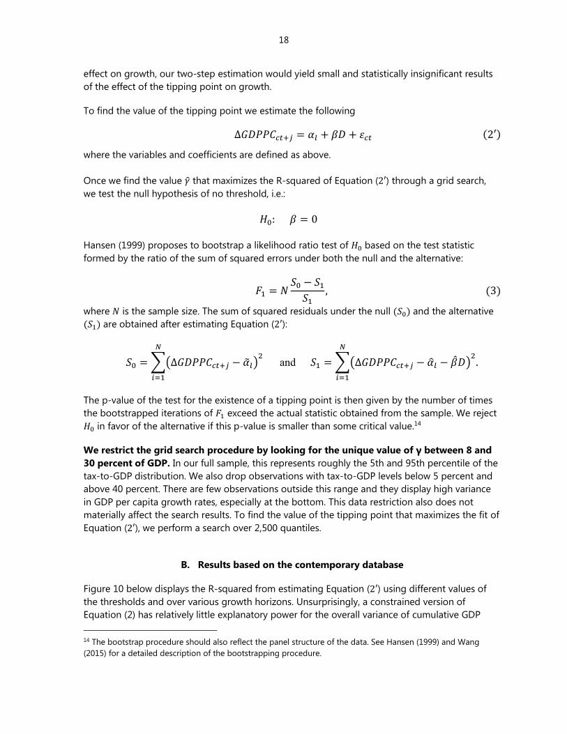
growth in our panel. The maximum R-squared reached is around 0.01 when using the 10-year

cumulative growth rate as dependent variable. However, the figure clearly suggests the existence

of a stable tipping point roughly halfway between 10 and 15 percent of GDP at all horizons

considered. In all cases, the series show a unique maximum although they are not strictly single-

peaked until 10 years. The threshold identified in Figure 10 is therefore a strong candidate for

estimating a tipping point in tax-to-GDP levels.

Figure 10. Searching for a Tax Tipping Point at Different Horizons

The figure displays the R-squared from estimating Equation (2′) when setting the estimated threshold γ̂ at

different values between 8 and 30 percent of GDP. The series are obtained using different growth horizons 𝑗= (3,

5, 7, 10) for the dependent variable. See text for details.

Next we test whether this threshold is statistically significant using the bootstrap

procedure proposed by Hansen (1999) and described above. The results are given in Table 2

below. The p-values of the estimated thresholds at all horizons are strongly statistically

significant well below the one percent level.15 This is consistent with the graphical evidence in

Figure 10, which shows a high degree of curvature around the single peaks for all series.

Beyond testing for the existence of a threshold, we also calculate confidence intervals for

our estimates so that we can assess how precisely to assign the structural break in GDP

growth to a specific tax level. Hansen (1999) provides further guidance for doing so. The

proposed method relies on a “no-rejection region” using the likelihood ratio statistic from

Equation (3). Intuitively, the idea is to delimit the confidence interval around the estimated

threshold �̂� to the range of values for which the difference between 𝑆(�̂�) and 𝑆1(𝛾) does not

exceed some critical value.16

15 As a robustness check, we also perform a similar bootstrap procedure using a cluster-robust Wald test statistic

for 𝐻0. The tipping point is significant at the 10 percent level at all horizons.

16 See Hansen (1999) for further details and critical values. Seijo and Sen (2011) also propose a smooth bootstrap

procedure. We find similar results with both methods, though confidence intervals using the smooth bootstrap

tend to be larger.

0

.002

.004

.006

.008

.01

R-s

qua

red

10 15 20 25 30Tax-to-GDP

3-year GDP growth 5-year GDP growth


20

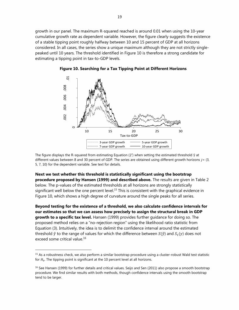
Table 2. Testing for Statistical Significance of Tax Thresholds

Dependent variable: GDP per capita cumulative growth

3-year 5-year 7-year 10-year

Hansen test statistic

p-value 0.000 0.000 0.000 0.000

F1 statistic 17.8 26.2 30.9 30.8

Critical values: 10% 2.8 3.2 2.7 2.6

5% 4.2 4.7 4.1 3.8

1% 6.6 7.5 6.9 5.7

Note: The table presents test statistics for the null hypothesis of no threshold in tax-to-GDP. p-

values and critical values are obtained by bootstrapping the individual test statistics 1000 times.

See text for further details about the construction of individual test statistics.

The point estimates for the tax threshold are consistent with the graphical evidence

presented in Figure 10 and are very stable across all horizons. The confidence intervals also

show that these threshold values are very precisely estimated. For example, the tax-to-GDP

threshold at the 10-year horizon has a point estimate of 12.88 percent and a 99 percent

confidence interval ranging from 11.33 percent of GDP to 13.97 percent, less than

2.65 percentage points wide. The confidence intervals are somewhat wider for shorter time

horizons. Because the confidence intervals do not rely on the usual Student or normal

distribution assumptions, they are also not necessarily symmetric. The observed asymmetry

derives from the specific shape of the series around their peak in Figure 10. In particular, the

slopes of the series are steeper to the right of their respective maximum so that the upper bound

of the confidence intervals will be closer to the estimated threshold than the lower bound.

Table 3. Estimated Tax-to-GDP Thresholds



Tax-to-GDP threshold 12.88 12.42 12.45 12.88

Confidence intervals:

No-rejection

region 95%

[11.56; 14.01] [11.70; 13.38] [11.60; 13.05] [11.62; 13.41]

99% [9.94; 14.19] [11.40; 13.78] [10.91; 13.51] [11.33; 13.97]

Note: The table presents estimates for the tax-to-GDP threshold using the specification search for

Equation (2′) described in the text. Confidence intervals are obtained by the “no-rejection region method. See

text for details.

Another important feature of the two-step estimator we use is the fact that is it super-

consistent, i.e. if one can reject the null, then the variance of the second step estimates

does not need to be corrected for the sampling error of the estimated threshold �̂� (Hansen

2000). From Table 2, we know we can confidently reject the null hypothesis that there is no

threshold, so we proceed with the regression discontinuity estimates from Equation (2) and use

the naïve standard errors as if the value of 𝛾 was known.

21

The effect of crossing the tax-to-GDP threshold on subsequent growth can be clearly

illustrated graphically. Figure 11 shows three estimators of the relation between tax levels and

growth: (1) average cumulative GDP per capita growth over 10 years within bins of bandwidth

equal to 0.517; (2) predicted values from a local linear regression with bandwidth of 1.5; and (3) a

global fourth-order polynomial in the level of tax-to-GDP fully interacted with the threshold

variable. The figure shows clearly the effect of the threshold at the point of discontinuity around

12.88 percent of GDP: countries that are immediately to the left of the tipping point on average

grow by around 20 to 25 percent in real terms over 10 years, or around 2 percent annually.

Countries immediately to the right of the threshold grow by more than 30 percent over 10 years,

or 2.8 percent annually. Both the local linear regression and the global fourth-order polynomial

provide very similar point estimates of the treatment effect �̂� at the point of discontinuity. It is

also interesting to note that the relationship between tax-to-GDP and growth is very noisy at the

bottom of the tax-to-GDP distribution. Right above the threshold, the relationship is smoother

with a slight negative slope beyond 15 percent of GDP. Appendix Table A1 lists the years in

which countries in the contemporary database cross the estimated threshold.

Figure 11. Impact of the Tax Threshold on 10-year Cumulative Growth

The scatter plot shows average GDP growth in 0.5-percentage-point bins. The solid line is a local linear regression

fit separately on either side of 12.88 using an Epanechnikov kernel and a bandwidth of 1.5. The dashed line is a

global fourth order polynomial estimated separately on either side of the tipping point. See text for further

details.

This regression discontinuity figure can be reproduced for all horizons and shows

consistently large treatment effects at the tax threshold.18 We show instead the effect on

growth of crossing the long-run discontinuity threshold of 12.88 percent for various time

horizons. Figure 12 plots estimates �̂� from Equation (2) excluding covariates and fixed effects,

where we vary the end year 𝑗 from 10 years prior to 15 years after the year we observe the tax to

17 Bins closest to the threshold contain over 140 country-year observations per bin.

18 See Appendix Figures A1-A3 for estimates using cumulative growth over 3, 5 and 7 years.

.1.2

.3.4

Cu

mu

lati

ve G

DP

gro

wth

5 10 15 20 25 30Tax-to-GDP

Local linear regression Fourth-order polynomial

Binned data

22

GDP ratio. The function 𝑓(𝑡𝑎𝑥𝑐𝑡) is estimated using a global fourth order polynomial. The figure

also shows the 90 percent confidence intervals to assess the statistical significance of the point

estimates across years.

Figure 12 shows the effect of crossing the threshold on GDP over time. The marginal effect

on growth increases smoothly over the first 10 years, then more sharply between years 10 and 13

before decreasing until 15 years after the year of observation. The difference between countries

that are initially just to the left of the tipping point in year 0 and those immediately to the right is

12.36 percent after 10 years and 16.85 percent 15 years later. This implies that crossing the tax

threshold adds about one percent to real annual GDP per capita growth for the next 10 to 15

years.

Another important feature of the approach is that it allows us to assess how countries on

either side of the tipping point differ in terms of growth rates in the years that precede

observation year 0. Finding systematic differences in growth rates for countries around the

threshold prior to the base year would cast serious doubt on the identification of a causal effect

of tax levels on growth. It is reassuring to find that no such pre-trend can be detected in the

figure. While some individual point estimates are statistically different from zero, a joint test of

the null that all pre-treatment coefficients are zero cannot be rejected at conventional levels (the

p-value of the test is 0.23). The point estimates are also smaller in magnitude than the cumulative

effect observed several years after the year of observation at year 0. Overall, this suggests that

the growth pattern of countries that were just to the left and just to the right of the tipping point

are very similar in the preceding years.

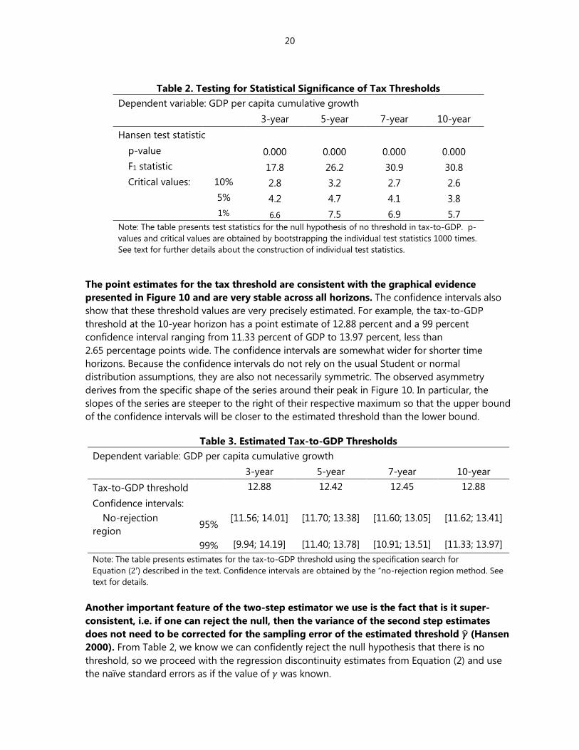
We also estimate the effect on GDP growth of crossing the tipping point in Equation (2)

under various specifications to assess the robustness of our regression discontinuity

estimate. Table 4 below presents the estimated coefficients for the tipping point 𝛽 when only a

global fourth-order polynomial in tax-to-GDP ratio fully interacted with the estimated tax-to-

GDP threshold at 12.88 is used in column (1). Column (2) adds country and year fixed effects,

while columns (3) to (7) add other variables typically used in cross-country growth regressions.19

19 See Hanushek and Woessmann (2015) for a recent example.

23

Figure 12. Impact of the Tax Threshold over Time

The figure plots estimate of β from Equation (2) estimated without covariates and fixed effects using cumulative

growth over horizons ranging from 10 years prior to 15 years after the year in which we observe the tax-to-GDP

ratio. Cumulative GDP per capita growth rates are calculated using year -1 as the base year. By construction they

are 0 in that year. The figure also plots the 90 percent confidence intervals. Standard errors are clustered at the

country level.

Column (1) reports the effect of the tax-to-GDP tipping point on cumulative GDP per

capita growth after 10 years. The point estimate is equal to the vertical distance at the point of

discontinuity shown in Figure 11. It is also equal to the point estimate reported in Figure 12 on

the full dynamic effect of the tipping point on growth at the 10-year mark. It indicates that

countries that are located immediately to the right of the tipping point of 12.88 percent of GDP

are 12.36 percent larger in real per capita terms on average than countries that are immediately

to the left. Adding country and year fixed effects reduces the estimated impact on cumulative

growth considerably, to 6.86 percent. Unsurprisingly, the overall R-squared increases markedly

from around 2 percent20 to 69 percent, with a within R-squared of 13.2 percent.

For our preferred specification in column (3), we add real GDP per capita in the initial year.

This increases the estimate of the impact of the threshold on growth, but only marginally, to

7.45 percent. The coefficient on GDP per capita itself is negative and strongly significant,

reflecting the usual convergence result in growth regressions. The R-squared once again

increases markedly to close to 74 percent for the overall and over 26 percent for the within R-

squared.

20 The R-squared in column (1) is twice as large as the maximum R-squared displayed in Figure 10 because of the

inclusion of the fully interacted fourth-order polynomial in tax-to-GDP level with the tax-to-GDP threshold.

0.1

.2.3

.4

Cu

mu

lati

ve im

pac

t o

n g

row

th

-10 -5 0 5 10 15Reference year

Treatment effect 90% CI

24

Table 4. Estimating Growth Effects

Dependent variable: 10-year cumulative GDP per capita growth

(1) (2) (3) (4) (5) (6) (7)

Tax-to-GDP threshold 12.355* 6.864** 7.450** 7.283** 6.852** 6.963** 7.717**

(6.651) (3.060) (3.017) (3.018) (3.081) (3.054) (2.967)

GDP per capita -3.127*** -2.972***

(0.538) (0.610)

Openness 7.644*** 4.388*

(2.762) (2.474)

Capital per capita 2.395 -13.893

(18.400) (16.755)

Human capital index -4.754 0.718

(4.170) (4.786)

Country and year FE No Yes Yes Yes Yes Yes Yes

Observations 3189 3189 3189 3189 3189 3189 3189

R-squared, overall 0.023 0.691 0.739 0.701 0.691 0.692 0.742

R-squared, within 0.132 0.266 0.159 0.132 0.135 0.275

Note: The table presents OLS results from Equation (2). The tax-to-GDP threshold is an indicator variable equal to one if the

tax level exceeds the estimated tipping point of 12.88 percent of GDP. GDP per capita is at constant national prices

expressed in thousands of 2005 US$. Capital stock and gross capital formation are expressed as a percent of GDP.

Openness is the sum of imports and exports as a percent of GDP. Human capital index is based on years of schooling and

returns to education. All data except tax-to-GDP ratios are taken from PWT 8.1. Coefficients from a fourth-order

polynomial in tax-to-GDP fully interacted with the tax-to-GDP threshold, year and country fixed effects not shown.

Standard errors clustered at the country level in parentheses. See text for details. * means p<10%, ** p<5%, *** p<1%.

In column (4) we replace GDP per capita with a variable reflecting the degree of openness

of the economy. This variable is simply the sum of imports and exports-to-GDP. Once again, the

coefficient for the tax-to-GDP threshold remains over 7 percent and the coefficient on the

degree of openness is also large and highly statistically significant. In column (5), we add instead

the total level of public and private capital per capita measured in 2005 US$. This leaves our main

threshold estimate broadly unchanged compared to column (2) with the coefficient associated

with capital not precisely estimated.

In column (6) we used human capital index as reported in the Penn World Tables. This leads

to a slightly higher estimate of the effect of the tipping point on cumulative GDP growth, with

the coefficient for the index itself not statistically significant.

Finally, in column (7) we include all control variables and fixed effects. The estimated

coefficients in all cases except for the degree of openness and human capital remain broadly

similar, including the estimated effect of the tax tipping point. Taken together, these results

confirm that our RDD estimate of the tax threshold is quite robust to the inclusion of important

determinants of growth.

25

Our analysis relies on a definition of tax revenues that excludes social security

contributions. This definition follows the classification standard adopted in the IMF’s 2014

Government Finance Statistics Manual. Unlike tax revenues, which are defined as compulsory and

unrequited amounts payable to the government, social security contributions are typically

associated with the expectation of future benefits. For this reason, associated revenues do not

change the net asset position of the government and are not freely usable for consumption or

investment.21

Exclusion of social security contributions from tax revenues also makes our two samples

more comparable. While complete information is not available for all countries in the

International Historical Statistics, comparison of the 1965-1980 time period, for which we have

overlap of data across the main estimation sample and the IHS data, shows that social security-

exclusive revenue series generally display higher correlation and more similar levels across the

two samples than social security-inclusive revenue series.

Finally, using social security-inclusive tax revenue series yields similar but consistently

lower results for the location of the tipping point. The estimates also vary more across

growth horizons. At the 10-year horizon, we estimate a tipping point at 12.0 percent of GDP. The

fact that we find a lower value for the tipping points is surprising given that mechanically one

would expect a higher tax threshold when including social contributions. For countries with tax

levels around the tipping point of 12.88 percent of GDP, social security contributions make up

around 10 percent of tax revenues. Therefore, if social contributions were not related to

subsequent economic growth, but were simply noise added to our tax series, one could expect a

tipping point to be found at around 14 percent of GDP.

We also find that the effect on subsequent growth is negligible and statistically

insignificant when using social security contribution-inclusive taxes and a value for the

tipping point of 12.0 percent. However, when the tipping point for these series is defined as

the sum of the contemporary database estimate of 12.88 percent of GDP plus the level of social

security contributions, we recover almost exactly our main estimate of the effect of the tax

threshold on subsequent GDP growth. We therefore conclude that adding social security

contributions to the definition of tax revenues does not provide additional information on the

location and effect of tax tipping points.

C. Results based on the historical database

One drawback of our contemporary database is that virtually all countries that were close

to or crossed the tax-to-GDP threshold of 12.88 percent during our sample period are

developing economies. Among OECD countries, only Spain and Turkey crossed this tipping

point since 1965. In order to assess whether advanced economies that are now well above the

threshold have also experienced similar tipping points during their development, we use

historical data on tax revenue and GDP from the International Historical Statistics (Mitchell 2003).

The starting year for the revenue and GDP series varies by country, but the longest series extends

21 It should be noted that the OECD’s Revenue Statistics include social security contributions in total taxes.

26

from 1800, for the United States until 1980. Summary statistics for our historical dataset are given

in Appendix Table A2.

We replicate the estimation procedure outlined above with our historical database.

Specifically, we perform a grid search over the values of revenue-to-GDP between 8 and

30 percent which maximizes the fit of Equation (2′) for various time horizons. The R-squared are

plotted in Figure 13. Similar to what we found with our contemporary database, there appears to

be a stable threshold not far from 12½ percent of GDP.

We perform the same tests for the existence of a threshold on the historical data.

Consistent with the visual evidence from Figure 13, we once again strongly reject the null

hypothesis of no threshold. We do not report the statistics in the interest of space, but once

again the p-values for both Hansen’s 𝐹1 statistic are well below 0.01. We report in Table 5 the

values of the estimated revenue threshold at 3, 5, 7 and 10 year horizons. We also report the “no-

rejection region” bootstrapped confidence intervals. Remarkably at all horizons, the estimated

value of the revenue-to-GDP threshold is 12.65 percent of GDP. This is very close to the

estimated threshold we found using our contemporary database.

Figure 13. Searching for a Tax Tipping Point at Different Horizons, Historical Database

The figure displays the R-squared from Equation (2′) when setting the estimated threshold γ̂ at different values

between 5 and 30 percent of GDP using the historical database. The series are obtained using different growth

horizons 𝑗 = (3, 5, 7, 10) for the dependent variable. See text for details.

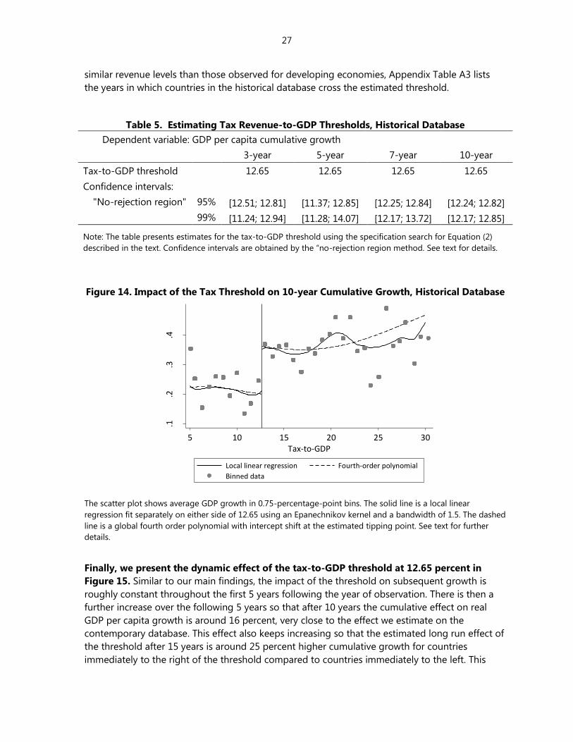
In Figure 14, we plot the effect of the revenue threshold on subsequent 10-year growth

rates. Similar to our main results presented in Figure 11, we observe a sharp increase in average

cumulative GDP per capita growth rates just above the estimated revenue threshold of

12.65 percent. This average growth rates remain higher than those observed at the lower end of

the revenue-to-GDP range, although the estimates are noisier than what we had in our

estimation using the contemporary database. This results suggest that advanced economies

underwent a similar structural break in revenue levels and that this changes occurred at strikingly

0

.02

.04

.06

.08

R-s

qu

ared

10 15 20 25 30Tax-to-GDP



27

similar revenue levels than those observed for developing economies, Appendix Table A3 lists

the years in which countries in the historical database cross the estimated threshold.

Table 5. Estimating Tax Revenue-to-GDP Thresholds, Historical Database



Tax-to-GDP threshold 12.65 12.65 12.65 12.65

Confidence intervals:

"No-rejection region" 95% [12.51; 12.81] [11.37; 12.85] [12.25; 12.84] [12.24; 12.82]

99% [11.24; 12.94] [11.28; 14.07] [12.17; 13.72] [12.17; 12.85]

Note: The table presents estimates for the tax-to-GDP threshold using the specification search for Equation (2)

described in the text. Confidence intervals are obtained by the “no-rejection region method. See text for details.

Figure 14. Impact of the Tax Threshold on 10-year Cumulative Growth, Historical Database

The scatter plot shows average GDP growth in 0.75-percentage-point bins. The solid line is a local linear

regression fit separately on either side of 12.65 using an Epanechnikov kernel and a bandwidth of 1.5. The dashed

line is a global fourth order polynomial with intercept shift at the estimated tipping point. See text for further

details.

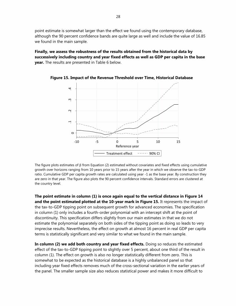
Finally, we present the dynamic effect of the tax-to-GDP threshold at 12.65 percent in

Figure 15. Similar to our main findings, the impact of the threshold on subsequent growth is

roughly constant throughout the first 5 years following the year of observation. There is then a

further increase over the following 5 years so that after 10 years the cumulative effect on real

GDP per capita growth is around 16 percent, very close to the effect we estimate on the

contemporary database. This effect also keeps increasing so that the estimated long run effect of

the threshold after 15 years is around 25 percent higher cumulative growth for countries

immediately to the right of the threshold compared to countries immediately to the left. This

.1.2

.3.4

Cu

mu

lati

ve G

DP

gro

wth

5 10 15 20 25 30Tax-to-GDP


Binned data

28

point estimate is somewhat larger than the effect we found using the contemporary database,

although the 90 percent confidence bands are quite large as well and include the value of 16.85

we found in the main sample.

Finally, we assess the robustness of the results obtained from the historical data by

successively including country and year fixed effects as well as GDP per capita in the base

year. The results are presented in Table 6 below.

Figure 15. Impact of the Revenue Threshold over Time, Historical Database

The figure plots estimates of β from Equation (2) estimated without covariates and fixed effects using cumulative

growth over horizons ranging from 10 years prior to 15 years after the year in which we observe the tax-to-GDP

ratio. Cumulative GDP per capita growth rates are calculated using year -1 as the base year. By construction they

are zero in that year. The figure also plots the 90 percent confidence intervals. Standard errors are clustered at

the country level.

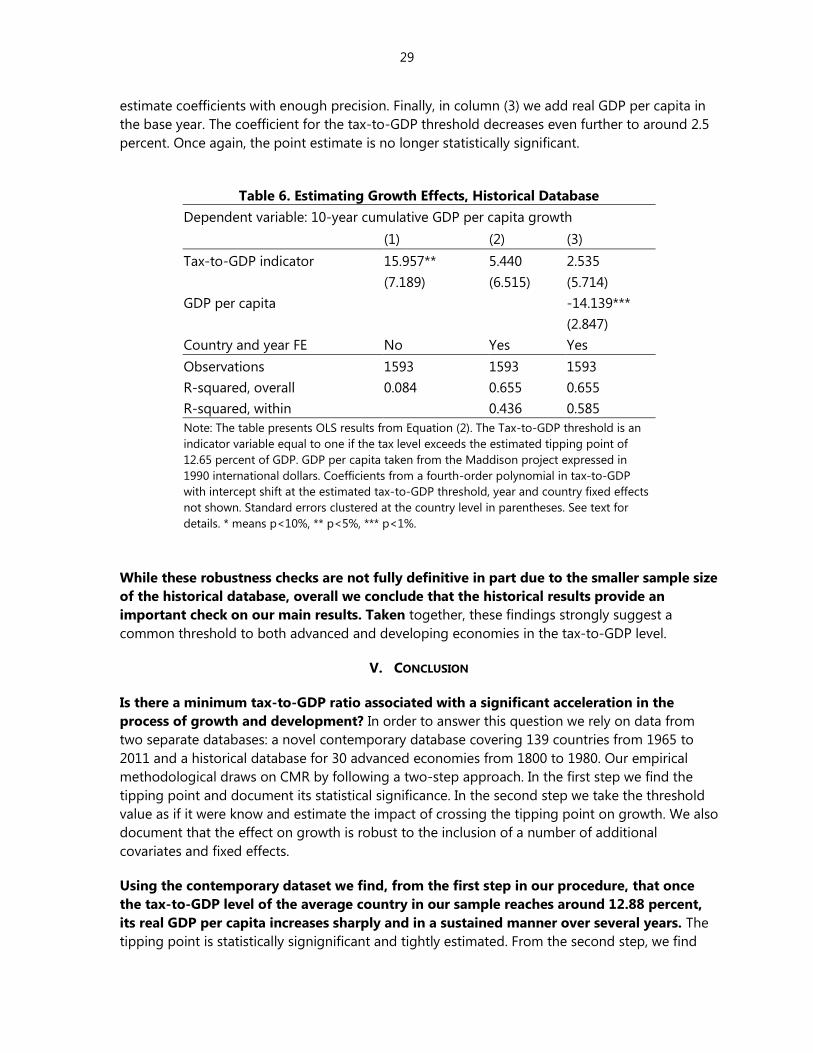
The point estimate in column (1) is once again equal to the vertical distance in Figure 14

and the point estimated plotted at the 10-year mark in Figure 15. It represents the impact of

the tax-to-GDP tipping point on subsequent growth for advanced economies. The specification

in column (1) only includes a fourth-order polynomial with an intercept shift at the point of

discontinuity. This specification differs slightly from our main estimates in that we do not

estimate the polynomial separately on both sides of the tipping point as doing so leads to very

imprecise results. Nevertheless, the effect on growth at almost 16 percent in real GDP per capita

terms is statistically significant and very similar to what we found in the main sample.

In column (2) we add both country and year fixed effects. Doing so reduces the estimated

effect of the tax-to-GDP tipping point to slightly over 5 percent, about one third of the result in

column (1). The effect on growth is also no longer statistically different from zero. This is

somewhat to be expected as the historical database is a highly unbalanced panel so that

including year fixed effects removes much of the cross-sectional variation in the earlier years of

the panel. The smaller sample size also reduces statistical power and makes it more difficult to

0.1

.2.3

.4

Cu

mu

lati

ve im

pac

t o

n g

row

th

-10 -5 0 5 10 15Reference year

Treatment effect 90% CI

29

estimate coefficients with enough precision. Finally, in column (3) we add real GDP per capita in

the base year. The coefficient for the tax-to-GDP threshold decreases even further to around 2.5

percent. Once again, the point estimate is no longer statistically significant.

Table 6. Estimating Growth Effects, Historical Database

Dependent variable: 10-year cumulative GDP per capita growth

(1) (2) (3)

Tax-to-GDP indicator 15.957** 5.440 2.535

(7.189) (6.515) (5.714)

GDP per capita -14.139***

(2.847)

Country and year FE No Yes Yes

Observations 1593 1593 1593

R-squared, overall 0.084 0.655 0.655

R-squared, within 0.436 0.585

Note: The table presents OLS results from Equation (2). The Tax-to-GDP threshold is an

indicator variable equal to one if the tax level exceeds the estimated tipping point of

12.65 percent of GDP. GDP per capita taken from the Maddison project expressed in

1990 international dollars. Coefficients from a fourth-order polynomial in tax-to-GDP

with intercept shift at the estimated tax-to-GDP threshold, year and country fixed effects

not shown. Standard errors clustered at the country level in parentheses. See text for

details. * means p<10%, ** p<5%, *** p<1%.

While these robustness checks are not fully definitive in part due to the smaller sample size

of the historical database, overall we conclude that the historical results provide an

important check on our main results. Taken together, these findings strongly suggest a

common threshold to both advanced and developing economies in the tax-to-GDP level.

V. CONCLUSION

Is there a minimum tax-to-GDP ratio associated with a significant acceleration in the

process of growth and development? In order to answer this question we rely on data from

two separate databases: a novel contemporary database covering 139 countries from 1965 to

2011 and a historical database for 30 advanced economies from 1800 to 1980. Our empirical

methodological draws on CMR by following a two-step approach. In the first step we find the

tipping point and document its statistical significance. In the second step we take the threshold

value as if it were know and estimate the impact of crossing the tipping point on growth. We also

document that the effect on growth is robust to the inclusion of a number of additional

covariates and fixed effects.

Using the contemporary dataset we find, from the first step in our procedure, that once

the tax-to-GDP level of the average country in our sample reaches around 12.88 percent,

its real GDP per capita increases sharply and in a sustained manner over several years. The

tipping point is statistically signignificant and tightly estimated. From the second step, we find

30

that, according to our preferred specification, a country just above the threshold will have real

GDP per capita around 7.5 percent larger, after 10 years, than an otherwise similar country just

below it. This effect is tightly estimated and economically large. In this specification we control

for country and time fixed effects as well as for the initial level of GDP per capita.

We also use a historical database, for 30 countries, going at most back to 1800. The

historical dataset allows the estimation of the tipping point for advances economies, as most of

them were already above the estimated threshold in 1965, when the contemporary database

starts. Remarkably, from the first step, we find a statistically significant threshold in government

tax revenue at 12.65 percent of GDP, very close to our result using contemporary data. The

tipping point is also tightly estimated. The threshold impact on subsequent growth is also

economically relevant, although not statistically significant, once time and country fixed effects

are introduced. While we lack the statistical power to find fully robust results on subsequent

growth in the historical sample, the coincidence of the threshold found in both databases, raises

the possibility that such a threshold is an invariant feature in the process of development. Hence

our answer to the initial question: “Is there a tipping point in the relation between tax capacity

and growth?” is yes!

From the estimates we obtained we think it is reasonable to assume a tax-to-GDP tipping

point at about 12 ¾ percent of GDP. As we said such threshold is likely associated with

changes in social norms of behavior and state capacity. Given that tax-to-GDP ratio are volatile

we think it is reasonable to interpret our findings as in line with the standard recommendation to

countries with low tax-to-GDP levels to aim for levels about 15 percent.

31

REFERENCES

Adam, C.S. and Bevan, D.L. (2005) “Fiscal Deficits and Growth in Developing Countries,” Journal of

Public Economics, 89, 571– 597.

Arezki, R., T. Gylfason, and A. Sy, 2011, Beyond the Curse: Policies to Harness the Power of

Natural Resources, Washington, DC: International Monetary Fund

Bai, J. (1997). “Estimation of a Change Point in Multiple Regression Models,” Review of Economics

and Statistics, 79, 551–563.

Barro, R. J., 1990, “Government spending in a simple model of endogenous growth”, Journal of

Political Economy, 98, 103-125.

Barro, R. J. and X. Sala-i-Martin, 1992, “Public finance models of economic growth”, Review of

Economic Studies, 59, 645-661.

Berg, A., Ostry, J. D., & Zettelmeyer, J. (2012). “What makes growth sustained?”, Journal of

Development Economics, 98(2), 149-166.

Brautigam, D., O. H. Fjeldstad, and M. Moore, 2008, Taxation and State-Building in Developing

Countries. Cambridge University Press

Benedek, D., E. Crivelli, S. Gupta, and P. Muthoora, 2014, “Foreign Aid and Revenue: Still a

Crowding Out Effect?”, Public Finance Analysis, Vol. 70 No. 1

Besley, T. and T. Persson, 2011, Pillars of Prosperity: The Political Economics of Development

Clusters. Princeton: Princeton University Press.

Besley, T. and T. Persson, 2013, “Taxation and Development”, Handbook of Public Economics,

Volume 5. Edited by A. J. Auerbach, R. Chetty, M. Feldstein and E. Saez. North Holland.

Besley, T. and T. Persson, 2014a, “Why do Developing Countries Tax so Little?”, Journal of

Economic Perspectives, Vol. 28, No. 4, Fall 2014, pages 99-120.

Besley, T. and T. Persson, 2014b, “The Causes and Consequences of Development Clusters: State

Capacity, Peace and Income”, Annual Review of Economics, 6:927-49.

Bird, R., J. Marinez-Vazquez, and B. Torgler, 2008, “Tax Effort in Developing Countries and High

Income Countries: The Impact of Corruption, Voice and Accountability”, Economic

Analysis and Policy, 38(1):55-71.

Burgess, R. and N. Stern, 1993, “Taxation and Development”, Journal of Economic Literature, Vol.

XXXI , pp. 762-830.

32

Caner, M. and B.E. Hansen, 2004, “Instrumental Variable Estimation of a Threshold Model,”

Econometric Theory, 20, 813-843.

Card, D., A. Mas, and J. Rothstein, 2008, “Tipping and the Dynamics of Segregation,” The

Quarterly Journal of Economics, 177-218.

Chudik, A., Mohaddes, K., Pesaran, M.H., and Raissi, M. (2015) “Is There a Debt-threshold Effect

on Output Growth,” IMF Working Paper No. 15/197

Ebeke, C. and Helene Ehrhart, 2011, “Tax Revenue Instability in Sub-Saharan Africa:

Consequences and Remedies”, Journal of African Economies, Vol. 21, number 1, pp. 1–27

Edwards, S., 2014, “Economic Development and the Effectiveness of Foreign Aid: A Historical

Perspective”, NBER Working Paper No. 20685, November

Feenstra, R. C., R. Inklaar and M. P. Timmer, 2015, "The Next Generation of the Penn World Table"

forthcoming American Economic Review, available for download at www.ggdc.net/pwt

Gordon, J.P.F., 1989. “Individual Morality and Reputation Costs as Deterrents to Tax Evasion,”

European Economic Review 33(4): 797–804.

Gordon, R., and W. Li, 2009, “Tax structures in developing countries: Many puzzes and a possible

explanation”, Journal of Public Economics, 93(7), 855-866.

Hansen, B.E. (1999) “Threshold Effects in Non-dynamic Panels: Estimation, Testing, and

Inference,” Journal of Econometrics, 93, 345-368.

Hansen, B. E. (2000), “Sample Splitting and Threshold Estimation,” Econometrica,

68, 575–603.

Hanushek, E. A., and Woessmann, L. (2015). The Knowledge Capital of Nations: Education and the

Economics of Growth. MIT Press.

Hausmann, R., Pritchett, L., & Rodrik, D. (2005), “Growth accelerations”, Journal of Economic

Growth, 10(4), 303-329.

International Monetary Fund, 2015, October 2015 Fiscal Monitor: The Commodities Roller

Coaster: A Fiscal Framework for Uncertain Times, Washington, D.C.: International

Monetary Fund

International Monetary Fund, 2015, Making Public Investment More Efficient.

Jensen, A. D., 2011, “State-Building in Resource-Rich Economies”, Atlantic Journal of Economics,

39:171–193

http://www.ggdc.net/pwt

33

Joshi, A., W. Prichard, and C. Heady, 2014, “Taxing the Informal Economy: The Current State of

Knowledge and Agendas for Future Research”, The Journal of Development Studies, Vol.

50, No. 10, 1325–1347

Kenny, L. W. and S. L. Winer, 2006, “Tax Systems in the World: An Empirical Investigaion into the

Importance of Tax Bases, Administration Costs, Scale and Political Regime”, International

Tax and Public Finance, 13 (2): 181-215.

Khan, M.S. and Senhadji, A.S. (2001) “Threshold Effects in the Relationship Between

Inflation and Growth,” IMF Staff Papers Vol. 48, No. 1.

Kiser, E., and M. Levi, 2015, “Interpreting the Comparative History of Fiscal Regimes”, Fiscal

Regimes and the Political Economy of Premodern States, edited by Andrew Monson and

Walter Sheidel, Cambridge University Press.

Kleven, H., C.T. Kreiner, and E. Saez, 2009, “Why Can Modern Governments Tax so Much? An

Agency Model of Girms as Fiscal Intermediaries”, NBER Working Paper No. 15218.

Laeven, L., and F. Valencia, 2012, “Systemic Banking Crises Database: An Update,” IMF Working

Paper No. 12/163

La Porta, R. and A. Shleifer, 2014, “Informality and Development”, Journal of Economic

Perspectives Volume 28, Number 3, pages 109–126

Lee, D.S.and T. Lemieux, 2010, “Regression Discontinuity Designs in Economics,” Journal of

Economic Literature, 48, 281–355

Levi, M. 1988. Of Rule and Revenue. Berkeley and Los Angeles, CA: University of California Press

Maddison-Project, http://www.ggdc.net/maddison/maddison-project/home.htm, 2013 version.

Mansour, M., 2014, “A Tax Revenue Dataset for Sub-Saharan Africa: 1980-2010”, Ferdi Working

Paper I19, July 2014

Mansour. M., 2015, “Tax Policy in MENA Countries: Looking Back and Forward”, IMF Working

Paper No. 15/98

Mitchell, B.R., 2003, International Historical Statistics: 1750–2000, 5th ed. Palgrave Macmillan,

Basingstoke.

Moore, M., 2007, “How does taxation affect the quality of governance?” Tax Notes International,

47, 79

Porter, J. and Yu, P., 2015, “Regression Discontinuity Designs with Unknown Discontinuity Points:

Testing and Estimation," Journal of Econometrics, 189, 132-147.

http://www.ggdc.net/maddison/maddison-project/home.htm

34

Posner, E. A., 2000, “Law and Social Norms: The Case of Tax Compliance.” Virginia Law Review

86(8, Symposium on the Legal Construction of Norms): 1781–1819

Pritchett, L., 2000a, “The tyranny of concepts: CUDIE (cumulated, depreciated, investment effort)

is not capital”, Journal of Economic Growth, 5, 361–384

Pritchett, L., 2000b, “Understanding patterns of economic growth: searching for hills

among plateaus, mountains, and plains”, World Bank Economic Review, 221–250.

Profeta, P. and S. Scabrosetti, 2010, The Political Economy of Taxation: Lessons from Developing

Countries, Elgar.

Reinhart, C. and K. Rogoff, 2008, “This Time is Different: A Panoramic View of Eight Centuries of

Financial Crises,” NBER Working Paper No. 13882

Ross, M., 2012, The Oil Curse: How Petroleum Wealth Shapes the Development of Nations,

Princeton: Princeton University Press.

Schumpeter, J.S., 1918, Die Krisis des Steuerstaats, Zeitfragen aus dem Gebiete der Soziologie, 4,

Graz and Leipzig: Leuschner & Lubensky, pp. 3-74 also available as chapter 1, The Crisis

of the Tax State, in Richard Swedberg (ed.), 1991, The Economics and Sociology of

Capitalism / Joseph A Schumpeter, Princeton:Princeton University Press.

Seidel, A., and M. Thum, 2015, “Tax Evasion, Corruption and Market Entry”, Scottish Journal of

Political Economy, doi: 10.1111/sjpe.12100

Seijo, E. and B. Sen, 2011, “Change-Point in Stochastic Design Regression and the Bootstrap,” The

Annals of Statistics, Vol. 39, No. 3, 1580–1607.

Slemrod, J. and S. Yitzhaki, 2002, “Tax Avoidance, Evasion, and Administration”, in A. Auerback

and M. Felstein (eds.) Handbook of Public Economics Vol 3. Amsterdam: Elsevier.

Tanzi, V., 1992, “Structural Factors and Tax Revenue in Developing Countries: A Decade of

Evidence”, Open Economies: Structural Adjustment and Agriculture. Edited by G. Ian and

L.A. Winters. Cambridge: Cambridge University Press.

Torgler, B., 2007, Tax Morale and Tax Compliance: A Theoretical and Empirical Analysis.

Cheltenham, UK: Edward Elgar.

Traxler, C., 2010, “Social Norms and Conditional Cooperative Taxpayers”, European Journal of

Political Economy, 26 (2010) 89–103.

Wang, Q., 2015, “Fixed-Effect Panel Threshold Model Using Stata,” Stata Journal, 15(1), 121–134.

35

Appendix

Figure A1. Impact of a Tax Threshold on 3-year Cumulative Growth



global fourth order polynomial estimated separately on either side of the estimated tipping point. See text for

further details.





further details.

0

.05

.1.1

5

Cu

mu

lati

ve G

DP

gro

wth

5 10 15 20 25 30Tax-to-GDP


Binned data

.05

.1.1

5.2

.25

Cu

mu

lati

ve G

DP

gro

wth

5 10 15 20 25 30Tax-to-GDP


Binned data

36





further details.

.1.1

5.2

.25

.3

Cu

mu

lati

ve G

DP

gro

wth

5 10 15 20 25 30Tax-to-GDP


Binned data

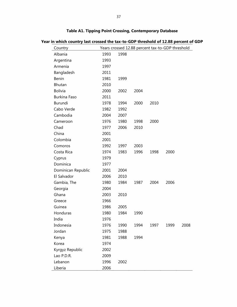
37

Table A1. Tipping Point Crossing, Contemporary Database

Year in which country last crossed the tax-to-GDP threshold of 12.88 percent of GDP

Country Years crossed 12.88 percent tax-to-GDP threshold

Albania 1993 1998

Argentina 1993

Armenia 1997

Bangladesh 2011

Benin 1981 1999

Bhutan 2010

Bolivia 2000 2002 2004

Burkina Faso 2011

Burundi 1978 1994 2000 2010

Cabo Verde 1982 1992

Cambodia 2004 2007

Cameroon 1976 1980 1998 2000

Chad 1977 2006 2010

China 2001

Colombia 2001

Comoros 1992 1997 2003

Costa Rica 1974 1983 1996 1998 2000

Cyprus 1979

Dominica 1977

Dominican Republic 2001 2004

El Salvador 2006 2010

Gambia, The 1980 1984 1987 2004 2006

Georgia 2004

Ghana 2003 2010

Greece 1966

Guinea 1986 2005

Honduras 1980 1984 1990

India 1976

Indonesia 1976 1990 1994 1997 1999 2008

Jordan 1975 1988

Kenya 1981 1988 1994

Korea 1974

Kyrgyz Republic 2002

Lao P.D.R. 2009

Lebanon 1996 2002

Liberia 2006

38

Year in which country last crossed the tax-to-GDP threshold of 12.88 percent of GDP

(continued)

Madagascar 1974 2008

Malawi 1978 1994 1997 2004

Maldives 1989 1991 2007 2011

Mali 1999 2002

Mauritania 1996 2005

Mexico 1983 1997 2000

Mozambique 1987 2009

Nepal 2010

Niger 2008

Panama 1983

Paraguay 2011

Peru 1994 2001 2003

Philippines 1990 2005

Portugal 1967 1976

Senegal 1987 1990 1995

Singapore 2007

South Africa 1973

Spain 1982

Sri Lanka 1973 1976 2004 2010

Suriname 1972 1995

Swaziland 1975 1977 1983 1988

São Tomé and

Príncipe 1982 2004

Tajikistan 2002

Thailand 1974 1979

Togo 1995 2003

Turkey 1992

Uruguay 1976 1980 1983 1985

Vietnam 1984 1988 1992

Zambia 2010

Zimbabwe 2010

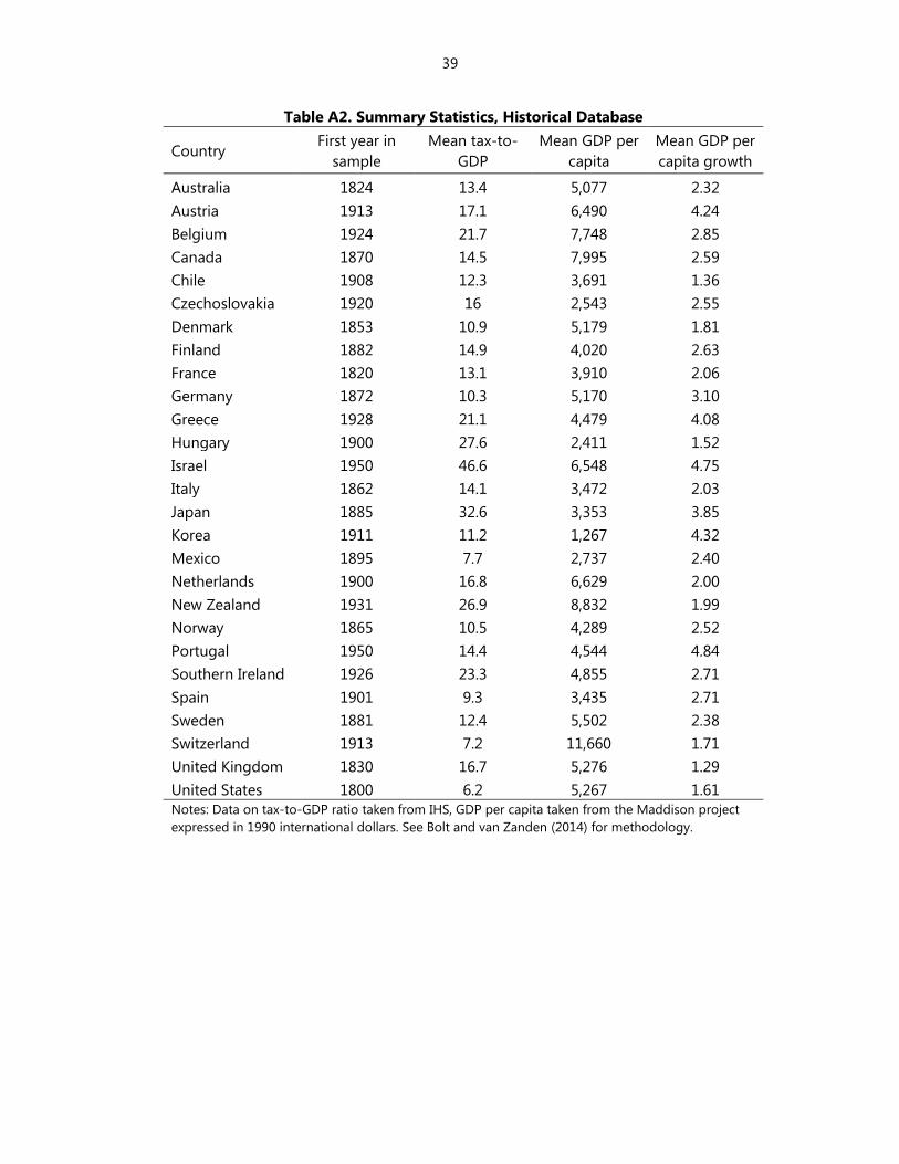
39

Table A2. Summary Statistics, Historical Database

Country First year in

sample

Mean tax-to-

GDP

Mean GDP per

capita

Mean GDP per

capita growth

Australia 1824 13.4 5,077 2.32

Austria 1913 17.1 6,490 4.24

Belgium 1924 21.7 7,748 2.85

Canada 1870 14.5 7,995 2.59

Chile 1908 12.3 3,691 1.36

Czechoslovakia 1920 16 2,543 2.55

Denmark 1853 10.9 5,179 1.81

Finland 1882 14.9 4,020 2.63

France 1820 13.1 3,910 2.06

Germany 1872 10.3 5,170 3.10

Greece 1928 21.1 4,479 4.08

Hungary 1900 27.6 2,411 1.52

Israel 1950 46.6 6,548 4.75

Italy 1862 14.1 3,472 2.03

Japan 1885 32.6 3,353 3.85

Korea 1911 11.2 1,267 4.32

Mexico 1895 7.7 2,737 2.40

Netherlands 1900 16.8 6,629 2.00

New Zealand 1931 26.9 8,832 1.99

Norway 1865 10.5 4,289 2.52

Portugal 1950 14.4 4,544 4.84

Southern Ireland 1926 23.3 4,855 2.71

Spain 1901 9.3 3,435 2.71

Sweden 1881 12.4 5,502 2.38

Switzerland 1913 7.2 11,660 1.71

United Kingdom 1830 16.7 5,276 1.29

United States 1800 6.2 5,267 1.61

Notes: Data on tax-to-GDP ratio taken from IHS, GDP per capita taken from the Maddison project

expressed in 1990 international dollars. See Bolt and van Zanden (2014) for methodology.

40

Table A3. Tipping Point Crossing, Historical Database

Country Years crossed 12.65 percent revenue-to-GDP threshold

Australia 1841 1892 1940

Canada 1940

Chile 1948 1951 1954 1957 1959

Czechoslovakia 1921

Denmark 1854 1863 1946 1955

Finland 1920 1934 1941

France 1879 1920

Germany 1934

Italy 1883 1887 1918 1949

Japan 1890 1895

Korea 1960 1962 1965

Netherlands 1917 1940

Norway 1946

Portugal 1956

Sweden 1943

United

Kingdom 1916

United States 1943

Notes: Data on tax-to-GDP ratio taken from IHS.

tax capacity and growth: is there a tipping point? - imf · tax capacity and growth: is there a...

Documents