tasopt engine model developmentpartner.mit.edu/sites/partner.mit.edu/files/report/file/... ·...

Partnership for AiR Transportation Noise and Emissions ReductionAn FAA/NASA/Transport Canada-sponsored Center of Excellence

TASOPT Engine Model Development

prepared byGiulia Pantalone, Elena de la Rosa Blanco, Karen Willcox

September 2016

REPORT NO. PARTNER-COE-2016-004

A PARTNER Project 48 report


A PARTNER Project 48 Report

Giulia Pantalone, Elena de la Rosa Blanco, Karen Willcox

PARTNER-COE-2016-004 September 2016

This work was funded by the US Federal Aviation Administration Office of Environment and Energy. The project was managed by James Skaleckyhe of the FAA.

Any opinions, findings, and conclusions or recommendations expressed in this material are those of the authors and do not necessarily reflect the views of the FAA, NASA, Transport Canada, the U.S. Department of Defense, or the U.S. Environmental Protection Agency

The Partnership for AiR Transportation Noise and Emissions Reduction — PARTNER — is a cooperative aviation research organization, and an FAA/NASA/Transport Canada-sponsored Center of Excellence. PARTNER fosters breakthrough technological, operational, policy, and workforce advances for the betterment of mobility, economy, national security, and the environment. The organization's operational headquarters is at the Massachusetts Institute of Technology.

The Partnership for AiR Transportation Noise and Emissions Reduction Massachusetts Institute of Technology, 77 Massachusetts Avenue, 33-240

Cambridge, MA 02139 USA partner.aero

1


Giulia Pantalone, Elena de la Rosa Blanco, Karen Willcox

This report describes the development of a new engine weight surrogate model and High Pressure Compressor (HPC) polytropic efficiency correction for the propulsion module in the Transport Aircraft OPTtimization (TASOPT) code. The goal of this work is to improve the accuracy and applicability of TASOPT in conceptual design of advanced technology, high bypass ratio, small-core, geared and direct-drive turbofan engines. The engine weight surrogate model was built as separate engine component weight surrogate models using least squares and Gaussian Process regression techniques on data generated from NPSS/WATE++ and then combined to estimate a “bare" engine weight—including only the fan, compressor, turbine, and combustor—and a total engine weight, which also includes the nacelle, nozzle, and pylon. The new model estimates bare engine weight within ±10% of published values for seven existing engines, and improves TASOPT's accuracy in predicting the geometry, weight, and performance of the Boeing 737-800. The effects of existing TASOPT engine weight models on optimization of D8-series aircraft concepts are also discussed. The HPC polytropic efficiency correction correlation, which reduces user-input HPC polytropic efficiency based on compressor exit corrected mass flow, was implemented based on data from Computational Fluid Dynamics (CFD). When applied to TASOPT optimization studies of three D8-series aircraft, the efficiency correction drives the optimizer to increase engine core size.

1 Introduction

The Federal Aviation Administration (FAA) Office of Environment and Energy (AEE) is developing tools to assess aircraft technologies and configurations, and to perform system-level uncertainty quantification (UQ) of coupled models. A process has been established for coupling Transport Aircraft System OPTimization (TASOPT) [1], a tool for conceptual aircraft design, with Aviation Environmental Design Tool (AEDT) Version 2a, a tool that calculates aircraft fuel burn. This coupled system is the focus of the UQ effort. Part of this work is to develop improved modeling capabilities within TASOPT. This report describes the development of a new engine weight model and the inclusion of engine size effects. Validation of the new TASOPT engine modeling capabilities is conducted and compared to data and existing tools.

1.1 Background and Motivation

The coupling of TASOPT and AEDT allows for fleet-wide analysis of advanced technology aircraft configurations with respect to fuel burn changes and the associated environmental impacts. An essential part of this capability is the accurate modeling of advanced technology aircraft by TASOPT. Thus, improving and expanding the applicability of TASOPT to other aircraft classes and engine types is valuable for future use of the TASOPT-AEDT coupled system. The rest of this section provides an overview of TASOPT and its integrated propulsion module.

1.1.1 TASOPT Background

2

TASOPT was developed by Drela at MIT for NASA's N+3 program to maximize transport efficiency by examining aircraft, engine, and fleet operation system designs, taking advantage of new technologies and a wider variety of configurations. It uses low-fidelity, physics-based models to accurately estimate weight, aerodynamic, and engine performance without the long computation time of higher-fidelity modeling techniques, such as Computational Fluid Dynamics (CFD) or Computational Structural Analysis (CSA). Historical correlations are only used in predicting engine weight and secondary structural weight. The drawback to using low-fidelity models is that TASOPT is currently restricted to tube-and-wing aircraft.

TASOPT can be executed in two modes: sizing mode and optimization mode. In sizing mode, TASOPT sizes the aircraft for a particular mission, i.e. range and payload. Similarly, in optimization mode, the aircraft is sized for a particular range and payload, but quantities such as cruise altitude, cruise lift coefficient, aspect ratio, wing sweep, engine fan pressure ratio, and engine bypass ratio (among others) are varied to minimize fuel consumption. Both modes can be run for a single mission or multiple missions. In multiple-mission sizing mode, the first mission is used to size the aircraft, which is then flown over the subsequent missions, evaluating the off-design performance. Optimization mode for multiple missions uses as its objective function the Payload Fuel Efficiency Index, or PFEI, which is the fuel energy consumption per payload-range. PFEI is calculated by weight-summing the fuel consumption of each mission specified. Thus, PFEI can be though of as a fleet-wide fuel consumption. TASOPT's capabilities allow the user to perform a variety of tasks, including

� Modeling an existing aircraft, evaluating its off-design performance, and performing sensitivity studies of various design parameters

� Analyzing the effects of advanced materials or engine technology on an airframe design

� Analyzing a strut-braced wing design or a geared or tail-mounted engine design, and

� Designing an entirely new aircraft for a set of missions.

1.1.2 TASOPT Propulsion Module

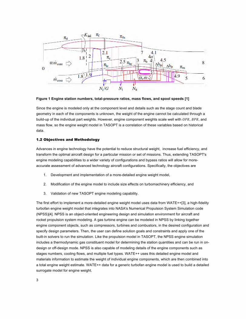
The propulsion model in TASOPT is a component-based thermodynamic cycle analysis as described by Kerrebrock [2] with variable specific heat based on a detailed gas-constituent model. Turbine cooling flow, which strongly influences optimal engine parameters, is also modeled and optimized for the takeoff case. On-design mode sizes the engine for cruise given a specified thrust 𝐹!"#, combustor exit temperature 𝑇!!, design fan pressure ratio 𝐹𝑃𝑅!, design overall pressure ratio 𝑂𝑃𝑅!, design bypass ratio 𝐵𝑃𝑅!, inlet kinetic energy defect 𝐾_𝑖𝑛𝑙, and the flight conditions. The output of sizing mode is the engine geometry (flow-path areas), corrected spool speeds, corrected mass flows, and cooling mass flow. In off-design mode, the performance of the engine during takeoff, climb, and descent is evaluated for either a specified thrust or a specified combustor exit temperature based on the engine geometry and spool speeds computed from an assumed fan or compressor map. Figure 1 provides a sketch of the component-based engine model in TASOPT.

3

Figure 1 Engine station numbers, total-pressure ratios, mass flows, and spool speeds [1]

Since the engine is modeled only at the component level and details such as the stage count and blade geometry in each of the components is unknown, the weight of the engine cannot be calculated through a build-up of the individual part weights. However, engine component weights scale well with 𝑂𝑃𝑅, 𝐵𝑃𝑅, and mass flow, so the engine weight model in TASOPT is a correlation of these variables based on historical data.

1.2 Objectives and Methodology

Advances in engine technology have the potential to reduce structural weight, increase fuel efficiency, and transform the optimal aircraft design for a particular mission or set of missions. Thus, extending TASOPT's engine modeling capabilities to a wider variety of configurations and bypass ratios will allow for more-accurate assessment of advanced technology aircraft configurations. Specifically, the objectives are

1. Development and implementation of a more-detailed engine weight model,

2. Modification of the engine model to include size effects on turbomachinery efficiency, and

3. Validation of new TASOPT engine modeling capability.

The first effort to implement a more-detailed engine weight model uses data from WATE++[3], a high-fidelity turbofan engine weight model that integrates into NASA's Numerical Propulsion System Simulation code (NPSS)[4]. NPSS is an object-oriented engineering design and simulation environment for aircraft and rocket propulsion system modeling. A gas turbine engine can be modeled in NPSS by linking together engine component objects, such as compressors, turbines and combustors, in the desired configuration and specify design parameters. Then, the user can define solution goals and constraints and apply one of the built-in solvers to run the simulation. Like the propulsion model in TASOPT, the NPSS engine simulation includes a thermodynamic gas constituent model for determining the station quantities and can be run in on-design or off-design mode. NPSS is also capable of modeling details of the engine components such as stages numbers, cooling flows, and multiple fuel types. WATE++ uses this detailed engine model and materials information to estimate the weight of individual engine components, which are then combined into a total engine weight estimate. WATE++ data for a generic turbofan engine model is used to build a detailed surrogate model for engine weight.

4

The second effort, which is to incorporate the effects of compressor size on turbomachinery efficiency, is accomplished by decreasing compressor polytropic efficiency as a function of compressor exit corrected mass flow based on trends quantified by DiOrio [5] using medium- and high-fidelity computational analysis. This correction to the compressor polytropic efficiency models losses observed in small compressors due to low chord Reynolds number and larger relative tip clearances compared to larger compressors. The compressor polytropic efficiency correction improves TASOPT’s ability to accurately model very high BPR (< 20) or low mass-flow turbofan engines.

Validation of the new engine model is performed separately for the engine weight model and compressor efficiency correction capability. The new engine weight model is validated by comparison to published engine weight data and other engine weight correlations. An analysis of the effects of different engine weight correlations on TASOPT models of a Boeing 737-800 and three conceptual advanced-technology aircraft is also presented. The compressor polytropic efficiency correction is also assessed by examining the effect of the correction on the optimization of the conceptual advanced-technology aircraft models.

2 Engine Weight Model Development

2.1 Current Model

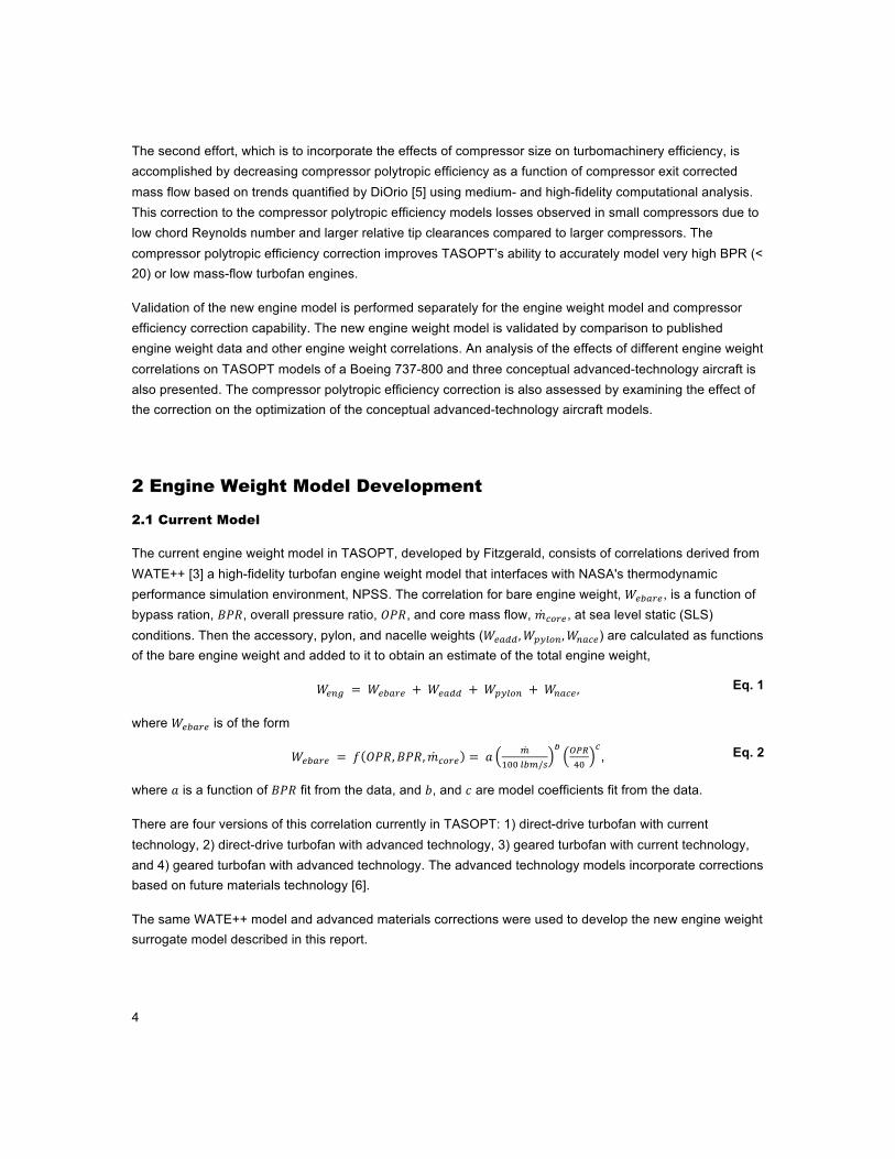
The current engine weight model in TASOPT, developed by Fitzgerald, consists of correlations derived from WATE++ [3] a high-fidelity turbofan engine weight model that interfaces with NASA's thermodynamic performance simulation environment, NPSS. The correlation for bare engine weight, 𝑊!"#$!, is a function of bypass ration, 𝐵𝑃𝑅, overall pressure ratio, 𝑂𝑃𝑅, and core mass flow, 𝑚!"#$, at sea level static (SLS) conditions. Then the accessory, pylon, and nacelle weights (𝑊!"## ,𝑊!"#$%,𝑊!"#$) are calculated as functions of the bare engine weight and added to it to obtain an estimate of the total engine weight,

𝑊!"# = 𝑊!"#$! + 𝑊!"## + 𝑊!"#$% + 𝑊!"#$ , Eq. 1

where 𝑊!"#$! is of the form

𝑊!"#$! = 𝑓 𝑂𝑃𝑅,𝐵𝑃𝑅,𝑚!"#$ = 𝑎 !!"" !"#/!

! !"#!"

!, Eq. 2

where 𝑎 is a function of 𝐵𝑃𝑅 fit from the data, and 𝑏, and 𝑐 are model coefficients fit from the data.

There are four versions of this correlation currently in TASOPT: 1) direct-drive turbofan with current technology, 2) direct-drive turbofan with advanced technology, 3) geared turbofan with current technology, and 4) geared turbofan with advanced technology. The advanced technology models incorporate corrections based on future materials technology [6].

The same WATE++ model and advanced materials corrections were used to develop the new engine weight surrogate model described in this report.

5

2.1.1 WATE++ Model Assumptions

WATE++ is based on a combination of historical component correlations and first principles-based component sizing and estimates the weight of the engine based on the station-by-station thermodynamic characteristics. The flow path cross-sectional areas can be calculated from the pressure, temperature, and mass flow at each station by assuming mass flow continuity. From this information, the blading requirements and number of stages for the fan, compressors, and turbines can then be characterized, and the weight of each stage estimated as a function of hub-to-tip ratio and material density. The weights of the disks, cases, and connecting hardware, and shaft weights follow from the blade weights and typical material properties. Most other components are estimated as a percentage of some other engine component weight.

Along with the station-by-station thermodynamic characteristics, the most important parameters to the WATE++ estimation of engine weight are 1) flow-path Mach number, 2) inlet hub-to-tip ratio for the Fan and High Pressure Compressor (HPC), 2) airfoil aspect ratio1, 3) blade volume factors, 4) blade solidity, and 5) blade loading [6]. In general, each of these parameters is different for each engine, but because the goal was to develop a correlation for engine weight with only 𝐵𝑃𝑅, 𝑂𝑃𝑅, and core mass flow as variables, Fitzgerald defined a “generic" engine model in WATE+ that would approximate the weight of various existing engines given an assumed set of parameters. The parameters of the generic engine model was calibrated using the following engines:

� CFM56-7B27

� V2530-A5

� PW2037

� PW4462

� PW4168

� PW4090

� GE90-85B

These engines range in SLS thrust from 27000 lbs to 85000 lbs and in 𝐵𝑃𝑅 from 4.6 to 8.5. Thus, they represent a large range of engine sizes. The calibrated parameters used in the generic WATE++ model are listed in Table 1 for the Fan, Low Pressure Compressor (LPC), High Pressure Compressor (HPC), High Pressure Turbine (HPT), and Low Pressure Turbine (LPT).

1 Airfoil aspect ratio is defined in WATE++ as the ratio of the span to the axial projection of the blade chord. Thus, the aspect ratio controls the axial length of each blade.

6

Table 1 Calibration Parameters [6]

Fan LPC HPC HPT LPT

Mach Number In 0.63 0.4 0.46 0.092 0.2

Mach Number Out 0.4 0.41 0.27 0.27 0.31

1st Stage Hub-to-Tip Ratio

0.325 0.59

Rotor Solidity 1.5 1.04 1.1 0.829 1.45

Stator Solidity 1 1.27 1.27 0.763 0.92

Rotor AR 2.73 1.5 – 2.2 1.5 – 2.2 1.0 – 2.0 1.0 – 8.0

Stator AR 4 2.3 – 3.1 2.3 – 3.1 Rotor/1.5 Rotor/1.2

Rotor Volume Factor

0.078 – 0.029 0.06 0.12 0.195 0.045

Stator Volume Factor

0.685 – 0.253 0.06 0.12 0.195 0.045

Blade Loading 0.25 0.19 0.31 1.2 1.5

Materials Ti-17 Ti-17 Ti-17,

Inconel 718

Hastelloy S, Rene 95

Inconel 718, Hastelloy S,

Rene 95, Udimet 700

Blade volume factor of the fan in the WATE++ model is a function of inlet mass flow, and thus there is a range of rotor and stator blade volume factors given in the table. The ranges given for aspect ratio denote that a variation of aspect ratio with span was used in the calibrated generic engine model. This is because smaller engines tend to have smaller blade aspect ratios in order to maintain higher Reynolds number flow, and assuming a constant value for all engines resulted in a bad fit.

7

Figure 2 Compressor aspect ratio variations with span [6].

Figure 3 Turbine aspect ratio variations with span [6].

The compressor aspect ratio trend was adapted from a previous implementation of WATE and is shown in Figure 2. Fitzgerald developed the turbine trends by examining published drawings of the calibration engines. The turbine aspect ratio trends are shown in Figure 3[6].

2.1.2 Advanced Materials Weight Reduction Methodology

The effect of advanced materials technology on engine weight was estimated by applying weight reductions to individual engine components and then recombining to get the total engine weight. The weight reductions used in Fitzgerald's models were used to develop the new engine weight models. These weight reductions, quantified as percent differences from current technology weight, were derived from published material from the MTU website, ASME and NASA publications [6], and communications with Pratt & Whitney subject matter experts. Details of the component weight reductions for advanced technology estimates are given in Table 2.

8

Table 2 Technologies for Weight Reduction [6]

Component Current Technology

Future Technology Weight Reduction Potential (% of

baseline)

References

Shafts Steel Alloys Metal Matrix Composites

30% MTU: Steffens and Wilhelm

Fan Blades Composite Titanium

More incorporation of composites

40-50% MTU: Steffens and Wilhelm

Fan Containment Alloys, composites Composites/Kevlar 30% NASA CR-2005-213969

Compressor Blades

Titanium/Nickel alloy

Titanium, Aluminide

components

30-40% MTU: Smarsly and P&W

Compressor Disk Titanium/Nickel Alloy

Titanium matrix composite rings

20-30% MTU: Smarsly 2008

HPT Blades Nickel Alloy Ceramic Matrix Composites

(CMC)

30-40% P&W

HPT Disk Nickel Alloy CMC 30-40% P&W

LPT Blades Nickel Alloy, present day stage

loading

50% stage loading increase, TiAL or CMC components

30% due to stage loading, 30% due

to materials

ASME GT2003-38374

MTU: Steffens and Wilhelm

LPT Disk Nickel Alloy 50% stage loading increase, TiAL or CMC components

30% due to stage loading, 30% due

to materials

ASME GT2003-38374

MTU: Steffens and Wilhelm

Fan drive gearbox Baseline Improved materials

10% P&W

Major frames Aluminum, Titanium, Nickel

Composites, Ceramics

20-30% P&W

Accessories Baseline Improved materials

10% P&W

9

2.2 Engine Breakdown

Instead of using a single correlation to estimate the bare engine weight, the engine was broken down into five separate components for which surrogate weight models were developed. These components are a) the core, including the LPC, HPC, HPT, LPT, and their adjoining ducts as well as accessories; b) the fan, including the bypass duct; c) the combustor; d) the nozzle, including the core and bypass nozzles; and e) the nacelle, which includes the inlet. Note that "accessories" accounts for the lubrication system, cooling system, instrumentation system, electrical system, actuation system, fuel pump and control system, and other configuration-specific items required to connect these systems to the engine2. The five component weight estimates are then added together to obtain the total engine weight.

W!"# = W!"#$ + W!"# + W!"#$%&'"( + W!"##$% + W!"#$%%$ Eq. 3

As with Fitzgerald's weight model, current and advanced technology surrogates were developed for both the direct drive and geared fan configurations, resulting in four sets of models. The data for these models were, again, generated from several thousand WATE++ simulations varying inlet mass flow, bypass ratio (𝐵𝑃𝑅), and overall pressure ratio (𝑂𝑃𝑅) at SLS. The ranges over which these input parameters were varied can be found in Table 3. The range of fan pressure ratio (𝐹𝑃𝑅) for each configuration, though not a design variable, is also included in the table. The gear ratio for the geared configuration, also an output of WATE++, varied based on the stress limits of the LPT blades or the Mach number limit of the LPC and ranged from 1.52 to 4.58.

Table 3 Design Variable Ranges for WATE++ Simulations

Variable Direct Drive Geared

𝑚!"#$% (lbm/s) [500, 3000] [500, 3000]

𝑂𝑃𝑅 [25, 60] [25, 60]

𝐵𝑃𝑅 [4, 15] [6, 30]

𝐹𝑃𝑅 [1.18, 1.80] [1.07, 1.80]

Once the data were generated from WATE++ for both the direct drive and geared configurations, weight reductions were applied to the separate components following Fitzgerald's method described in Section 1.2. The final ranges of percent total engine weight for each component in the four sets of surrogate models are in Table 4. Note that the component percent total engine weights do not differ very much between current and advanced technology because the weight reductions are small compared to the component weights.

2 From communication with Michael Tong, NASA Glenn Research Center

10

Table 4 Component Percentage of Total Engine Weight

Component Direct Drive Current Tech.

Direct Drive Advanced Tech.

Geared Current Tech.

Geared Advanced Tech.

Core 45.0 – 65.3 % 43.5 – 62.9% 28.4 – 57.4% 26.7 – 55.1%

Fan 13.2 – 22.9% 13.1 – 22.9% 18.5 – 38.7% 18.6 – 38.9%

Combustor 0.87 – 4.7% 0.99 – 4.9% 1.2 – 3.8% 1.2 – 3.9%

Nozzle 7.6 – 22.1% 7.8 – 22.3% 9.9 – 26.5% 10.3 – 26.8%

Nacelle 8.0 – 18.9% 8.6 – 19.5% 8.7 – 15.1% 9.2 – 15.5%

2.3 Sensitivity Analysis

Prior to developing the surrogate models, Global Sensitivity Analysis (GSA) was performed to determine the most important variables and the level of interactions between variables in the NPSS/WATE++ model. The Monte-Carlo based Sobol' method [7][8] was used to calculate the main effect sensitivity indices and total effect sensitivity indices of each variable for each engine component. The main effect sensitivity index, 𝑆!, of the 𝑖!! input variable can be best understood as a measure of the variance of the system output caused by the 𝑖!! variable alone, i.e. the “importance" of that variable. The total effect sensitivity index, 𝑆!!, is a measure of the total contribution to the output variance of the system by the 𝑖!! variable, including its main effect on the system plus the effects of interactions between the 𝑖!! variable and the other variables. Thus, the difference between the total effect index and main effect index for a given variable is an indication of how much the variable interacts with other inputs to the system.

To calculate the sensitivity indices, 10,000 uniformly distributed quasi-Monte Carlo samples of 𝑂𝑃𝑅, 𝐵𝑃𝑅, and inlet mass flow were propagated through WATE++ to obtain component weight outputs. The input distributions were drawn from the Sobol' sequence, which is a quasi-random low-discrepancy deterministic sequence that distributes samples more uniformly throughout the design space than would a pseudo-random Monte Carlo sampling scheme. This allows the calculation of the sensitivity indices to converge with fewer samples. The process was repeated for both the direct drive and geared configurations. The block diagram in Figure 4 depicts the propagation of uncertainty through the NPSS/WATE++ model. The notation 𝑋 ∼ 𝑈 𝑎, 𝑏 defines 𝑋 as a random variable whose value is uniformly distributed between the values 𝑎 and 𝑏.

Figure 4 Block diagram of uncertainty propagation through NPSS/WATE++

The results of the GSA for each configuration (direct drive and geared with current or advanced technology)

11

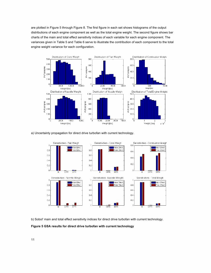
are plotted in Figure 5 through Figure 8. The first figure in each set shows histograms of the output distributions of each engine component as well as the total engine weight. The second figure shows bar charts of the main and total effect sensitivity indices of each variable for each engine component. The variances given in Table 5 and Table 6 serve to illustrate the contribution of each component to the total engine weight variance for each configuration.

a) Uncertainty propagation for direct drive turbofan with current technology.

b) Sobol' main and total effect sensitivity indices for direct drive turbofan with current technology.

Figure 5 GSA results for direct drive turbofan with current technology

12

a) Uncertainty propagation for direct drive turbofan with advanced technology.

b) Sobol' main and total effect sensitivity indices for direct drive turbofan with advanced technology.

Figure 6 GSA results for direct drive turbofan with advanced technology.

13

a) Uncertainty propagation for geared turbofan with current technology.

b) Sobol' main and total effect sensitivity indices for geared turbofan with current technology.

Figure 7 GSA results for geared turbofan with current technology

14

a) Uncertainty propagation for geared turbofan with advanced technology.

b) Sobol' main and total effect sensitivity indices for geared turbofan with advanced technology.

Figure 8 GSA results for geared turbofan with advanced technology

For the direct drive turbofan, inlet mass flow is the most important variable to the total engine weight, as well as the core, fan, nozzle, and nacelle weights. Inlet mass flow and 𝐵𝑃𝑅 are both important for the combustor weight. Furthermore, the combustor and nozzle are the only components for which there are significant interactions between design variables. As mentioned previously, the effect of interactions between one variable and the other variables is the difference of the total effect index and the main effect index

15

corresponding to that variable. For example, from Figure 5, the interaction effect for inlet mass flow on the combustor weight is the difference between the red bar and the blue bar, that is

𝑆!,!"#$%&'#!(" = 𝑆!! − 𝑆! = 0.532 − 0.445 = 0.077 Eq. 4

These observations hold for both the current and advanced technology configurations. Only small adjustments relative to total component weight were made to the core, fan, and combustor weights in the advanced technology model, resulting in only small differences in variance between the current and advanced technology versions of those components.

The fact that bypass ratio is not an important variable for the fan weight might seem non-intuitive, but this is because, in general, the NPSS/WATE++ model increases bypass ratio by reducing the size of the core rather than increasing the size of the fan. It may also be surprising that overall pressure ratio is the least important variable for all engine components; this is likely because the effect of inlet mass flow overwhelms the effects of the other two variables.

Table 5 Direct-drive Component Weight Distribution Variances

Component 𝜎!"##$%& [lb] 𝜎!"#!$%&" [lb]

Core 3004.8 2895.9

Fan 984.7 975.3

Combustor 164.6 164.6

Nozzle 1248.6 1248.6

Nacelle 402.4 402.4

Total Engine 5628.7 5511.2

For the geared turbofan, all engine components have at least two variables that are important. Additionally, bypass ratio is the dominant variable for the combustor and core weights in the geared configuration. There are also larger interactions between variables in the geared model than in the direct drive model, which can bee seen from the larger difference between the red and blue bars in Figure 7 and Figure 8 as compared to Figure 5 and Figure 6. Note that the fan weight and total engine weight for the geared configuration have larger variances than the direct drive configuration due to the larger variance in the input distribution of 𝐵𝑃𝑅.

Table 6 Geared Component Weight Distribution Variances

Component 𝜎!"##$%& [lb] 𝜎!"#!$%&" [lb]

Core 1409.3 1386.1

Fan 1055.2 1047.8

16

Combustor 134.1 134.1

Nozzle 787.0 787.0

Nacelle 403.1 403.1

Total Engine 3439.4 3340.7

2.4 Surrogate Models

2.4.1 Model Types

Two types of surrogate modeling techniques were used to create the new engine weight model in TASOPT: Least Squares (LS) regression and Gaussian Process (GP) regression [9]. LS regression fits a 2nd, 3rd, or 4th order polynomial of three variables to the data, which makes it suitable for smooth objective functions. A GP, on the other hand, interpolates the data, making it a more suitable approach for multi-modal functions. However, GPs are more computationally expensive to use and create than polynomial correlations. Most of the engine component weight functions are smooth and the LS models are sufficiently accurate. For the multi-modal engine component weight functions, a GP was used.

2.4.2 Cross-Validation

The 5-fold cross-validation method was use to validate the models presented in the following sections. In this method, the original sample data is divided into five equal size sets. Four of the sets are used to train the model and the remaining set is used for testing. This process is repeated for all possible combinations of training and test data (five combinations). If the fit parameters and error statistics are acceptable and consistent among the five rounds, then the number of samples being used to train the model is likely to be sufficient. All of the models presented in the following sections were cross-validated with an original data set of 2500 samples. This size data set was chosen because models built using all 10,000 samples did not show any improvement in accuracy and, in the case of the GP models, took significantly more time to build.

2.4.3 Direct-Drive Turbofan, Current Materials

A full factorial design of experiments (DOE) was run in NPSS/WATE++ with eight levels of 𝑂𝑃𝑅, seven levels of 𝐵𝑃𝑅, and six levels of 𝑚!"#$% to generate 336 samples that were used to build surface plots of the objective functions. The same design variable ranges used in the GSA were used for the DOE. The fan, combustor, nozzle, and nacelle weight functions were smooth, so polynomial functions were fit to the data using the least squares method. The core weight function was multi-modal, so a GP was used instead of a polynomial fit. All models used 𝑂𝑃𝑅, 𝐵𝑃𝑅 and 𝑚!"#$ as input variables, except for the fan weight model, which uses 𝑚!"#$% instead of 𝑚!"#$Technically, these variables are interchangeable since they are related by equation,

𝑚!"#$ =!!"#$%

! ! !"#, Eq. 5

but since inlet mass flow is directly related to the size of the fan, a better fit was obtained using inlet mass flow as the input variable. Once the model types were chosen for each component---either a GP model or a

17

certain degree polynomial fit---cross-validation was performed and final models were built using the Sobol' sequence samples from the GSA study. A quadratic LS model was sufficient for the combustor weight model, whereas the fan and nacelle weight models required cubic LS models. The nozzle weight had two modes, i.e. it had two peaks, and required a quartic LS model. A GP model was also explored for the nozzle weight, but maximum errors did not improve, so the quartic polynomial was chosen for computational efficiency. The final model types and error statistics are summarized in Table 7 and Table 8. The tables list percent error and absolute errors respectively.

We define percent model error as

𝑒𝑟𝑟𝑜𝑟 = ! ! !!"#

! × 100. Eq. 6

where 𝑊 is the value from NPSS/WATE++ and 𝑊!"# is the value given by the LS or GP model. The goal was to have model errors less than 10%. Though the maximum error for some of the models is around 10% or higher, the mean and median errors for these models is low, indicating a low incidence of model errors greater than 10%. The nozzle weight surrogate, for example, has a maximum error of 23.7%, but the mean and median errors are around 1%. The large errors at a few points are due to noise in the data used to fit the model. As we will see later, these high error points are located at the edges of the design space.

Table 7 Direct Drive Current Technology Model Error

Component Type Mean Error [%] Max Error [%] Median Error [%]

Core Cubic LS 3.17 10.3 2.77

Fan GP 1.47 6.59 1.25

Combustor Quadratic LS 0.37 6.87 0.25

Nozzle Quartic LS 1.2 23.7 1.03

Nacelle Cubic LS 0.91 5.61 0.74

Table 8 Direct Drive Current Technology Absolute Model Errors

Component Type Mean Error [lb] Max Error [lb] Median Error [lb]

Core Cubic LS 72.4 249.6 66.0

Fan GP 113.6 600.4 92.1




18

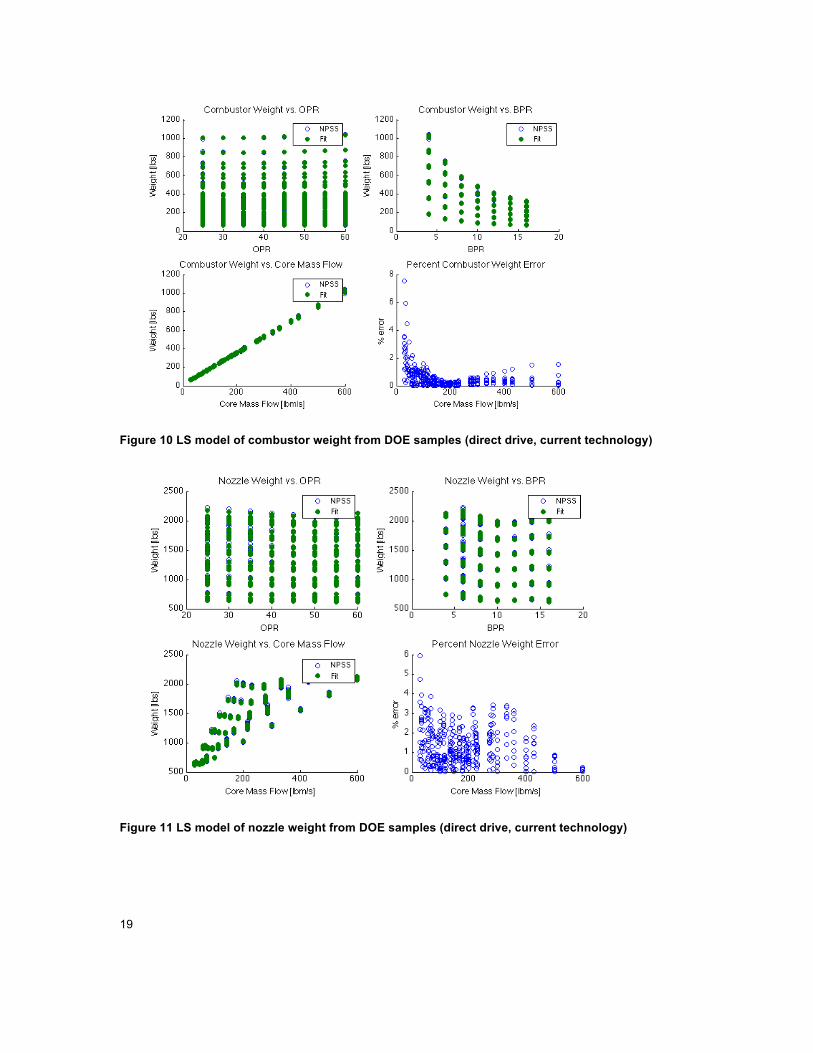
Figure 9 through Figure 10 contain scatter plots of output data from the least squares model along with the training data points from NPSS/WATE++. The bottom right-hand plot in each figure shows the percent error of the model predictions calculated as in Eq. 6. Figure 13 is a surface plot of the GP model for the core weight with the data from NPSS plotted in blue dots over the surface. The models that these plots represent were built using data from the DOE, and thus they are not the final models that are included in TASOPT, but they are good visualizations of the shapes of the weight functions. Note that the maximum errors in Figure 9 through Figure 12 differ from the maximum errors of the final models given in Table 7 because a few of the 2500 NPSS/WATE++ solutions used to build the final models were unconverged.

Figure 9 LS model of fan weight from DOE samples (direct drive, current technology)

19

Figure 10 LS model of combustor weight from DOE samples (direct drive, current technology)

Figure 11 LS model of nozzle weight from DOE samples (direct drive, current technology)

20

Figure 12 LS model of nacelle weight from DOE samples (direct drive, current technology)

Figure 13 GP model of core weight from DOE samples (direct drive, current technology). The six surfaces are levels of constant inlet mass flow from 500 lbm/s to 3000 lbm/s. The color corresponds to weight, with blue being the lowest weight and red the highest.

Since some large errors were observed in the nozzle weight model, it is important to know if these errors are random noise or localized to a certain part of the design space. In Figure 14, 2500 test samples are plotted with blue indicating designs with less than 2% error, green indicating designs with error between 2% and 5%, and red for points with greater than 5% error. It is clear from the plot that the high error points are

21

localized to higher values of 𝐵𝑃𝑅. The highest bypass ratio engine currently in existence has a bypass ratio around 11, which is well within the low error region of the surrogate model. Caution will be necessary when using this model to predict weight for direct drive engines with bypass ratios closer to 15, though the user would likely use a geared turbofan engine in this case.

Figure 14 Scatter plots of nozzle weight error (direct drive, current technology)

2.4.4 Direct-Drive Turbofan, Advanced Materials

The advanced technology models were built using the same procedure as the current technology models. First, the DOE samples were used to determine the correct model type, and then the final models were built using the randomized samples from the GSA. Since the difference between the current and advanced technology data is small relative to the component weights, the model types that were appropriate for each component are the same in both cases. The error statistics are also very similar between the two sets of models. A summary of the direct drive advanced technology models can be found in Table 9 and Table 10.The tables list percent error and absolute errors respectively.

Table 9 Direct Drive Advanced Technology Model Error


Core Cubic LS 1.53 7.14 1.29

Fan GP 1.63 5.50 1.43




22

Table 10 Direct Drive Advanced Technology Absolute Model Errors


Core Cubic LS 109.0 566.0 87.7

Fan GP 95.0 353.0 73.4




Figure 15 through Figure 18 contain scatter plots of output data from the least squares model along with the training data points from NPSS/WATE++. The bottom right-hand plot in each figure shows the percent error of the model predictions calculated as in Eq. 6. As with the direct drive current technology plots, the maximum errors in the following plots do not match the errors in Table 9 Direct Drive Advanced Technology Model Error because of some unconverged solutions in the data used to build and test the final models.

Figure 15 LS model of fan weight from DOE samples (direct drive, advanced technology)

23

Figure 16 LS model of combustor weight from DOE samples (direct drive, advanced technology)

Figure 17 LS model of nozzle weight from DOE samples (direct drive, advanced technology)

24

Figure 18 LS model of nacelle weight from DOE samples (direct drive, advanced technology)

As in the current technology models, errors larger that 10% were observed in the advanced technology nozzle weight model. In Figure 19 we see that the higher errors occurred for bypass ratios close to 15, similar to the current technology case.

Figure 19 Scatter plots of nozzle weight error (direct drive, advanced technology)

2.4.5 Geared Turbofan, Current Materials

For the geared configuration, a DOE of 624 samples was generated. As seen in the sensitivity analysis, there is more complexity in the geared turbofan component weights than in the direct drive case. Thus, more-complex model types were required. Cubic polynomial fits were used for the fan, combustor, and nacelle weight models, whereas GP models were required for the core and nozzle. Due to the complexity of

25

the geared turbofan system relative to the direct drive system, larger errors are observed in the surrogate models. Table 11 and Table 12 list percent error and absolute error respectively.

Table 11 Geared Current Technology Model Error


Core Cubic LS 3.19 11.9 2.81

Fan GP 1.00 7.74 0.67

Combustor Cubic LS 0.28 4.81 0.15

Nozzle GP 1.21 47.7 0.77


Table 12 Geared Current Technology Absolute Model Errors


Core Cubic LS 78.8 274.2 74.4

Fan GP 32.6 417.6 21.6


Nozzle GP LS 17.5 840.7 9.53


Figure 20 through Figure 22 contain scatter plots of output data from the least squares model along with the training data points from NPSS/WATE++. The bottom right-hand plot in each figure shows the percent error of the model predictions calculated as in Eq. 6. As was the case in the direct drive plots, the maximum errors in the following plots do not match the errors in Table 11 because of some unconverged solutions in the data used to build and test the final models.

26

Figure 20 LS model of fan weight from DOE samples (geared, current technology)

Figure 21 LS model of combustor weight from DOE samples (geared, current technology)

27

Figure 22 LS model of nacelle weight from DOE samples (geared, current technology)

For the geared turbofan, both the nozzle and nacelle models had errors much larger than 10%. Figure 23 shows design points with less than 10% error in blue, between 10% and 20% error in green, and greater than 20% error in red. The high error design points seem to follow a trend in the 𝐵𝑃𝑅 vs. 𝑂𝑃𝑅 plot, indicating that NPSS/WATE++ does not converge properly for those combinations of inputs. In Figure 24, in which blue dots are for design points with error less than 5%, green for error between 5 and 10%, and red for error greater than 10%, the high error region is localized to low values of mass flow.

Figure 23 Scatter plots of nozzle weight error (geared, current technology)

28

Figure 24 Scatter plots of nacelle weight error (geared, current technology)

2.4.6 Geared Turbofan, Advanced Materials

As in the current technology case, cubic polynomial fits were used for the fan, combustor, and nacelle weight models, and GP models were used for the core and nozzle. Similar maximum errors were observed as well, though the mean and median errors continue to be low, indicating that the high errors are due to noise in the NPSS/WATE++ outputs. Table 13 and Table 14 list percent error and absolute error respectively.

Table 13 Geared Advanced Technology Model Error


Core Cubic LS 3.19 11.4 2.81

Fan GP 1.03 7.56 0.69


Nozzle GP 1.17 46.9 0.71


Table 14 Geared Advanced Technology Absolute Model Errors


Core Cubic LS 78.1 271.6 73.8

Fan GP 30.5 391.7 20.3


Nozzle GP LS 17.1 826.6 8.85


29

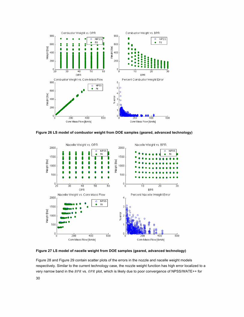
Figure 25 through Figure 27 contain scatter plots of output data from the least squares model along with the training data points from NPSS/WATE++. The bottom right-hand plot in each figure shows the percent error of the model predictions calculated as in Eq. 6. As was the case in the current technology plots, the maximum errors in the following plots do not match the errors in Table 13 because of some unconverged solutions in the data used to build and test the final models.

Figure 25 LS model of fan weight from DOE samples (geared, advanced technology)

30

Figure 26 LS model of combustor weight from DOE samples (geared, advanced technology)

Figure 27 LS model of nacelle weight from DOE samples (geared, advanced technology)

Figure 28 and Figure 29 contain scatter plots of the errors in the nozzle and nacelle weight models respectively. Similar to the current technology case, the nozzle weight function has high error localized to a very narrow band in the 𝐵𝑃𝑅 vs. 𝑂𝑃𝑅 plot, which is likely due to poor convergence of NPSS/WATE++ for

31

those combinations of inputs. Again, high error for the nacelle weight occurs mostly at low values of mass flow.

Figure 28 Scatter plots of nozzle weight error (geared, advanced technology)

Figure 29 Scatter plots of nacelle weight error (geared, advanced technology)

2.5 Engine Weight Model Validation

To validate the new engine weight model, we first compare the bare engine weight estimates to published data. Next, the integrated engine weight model in TASOPT is assessed by modeling four aircraft and comparing the predicted performance with each engine weight model.

2.5.1 Comparison to Published Data

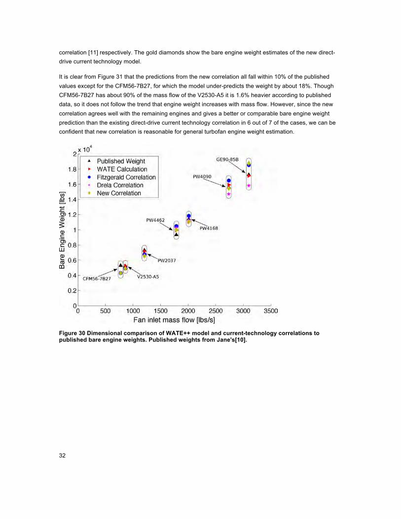
In order to determine if the new engine weight model is providing appropriate estimates, the weights of the seven engines used to calibrate the WATE++ model were estimated using the new engine weight surrogate and then compared to published data, the WATE++ model calculation, and estimates from the existing correlations in TASOPT. The bare engine weight is the combined weight of the core (compressors, combustor, and turbines) and fan, and does not include the nacelle, nozzle, or pylon weight. The weight of these components is not publicly available. The comparison is shown dimensionally in Figure 30 and as a percentage of the published value in Figure 31. In the figures, the black triangles represent the published weight of each engine from Jane's[10] and the red triangles show the WATE++ calculated value[6]. The blue circles and magenta stars represent Fitzgerald's direct-drive current technology correlation [6] and Drela's

32

correlation [11] respectively. The gold diamonds show the bare engine weight estimates of the new direct-drive current technology model.

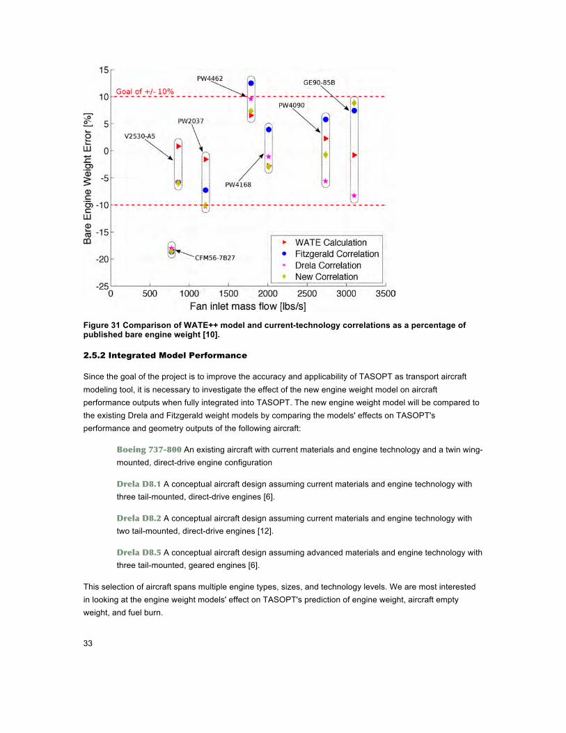
It is clear from Figure 31 that the predictions from the new correlation all fall within 10% of the published values except for the CFM56-7B27, for which the model under-predicts the weight by about 18%. Though CFM56-7B27 has about 90% of the mass flow of the V2530-A5 it is 1.6% heavier according to published data, so it does not follow the trend that engine weight increases with mass flow. However, since the new correlation agrees well with the remaining engines and gives a better or comparable bare engine weight prediction than the existing direct-drive current technology correlation in 6 out of 7 of the cases, we can be confident that new correlation is reasonable for general turbofan engine weight estimation.

Figure 30 Dimensional comparison of WATE++ model and current-technology correlations to published bare engine weights. Published weights from Jane's[10].

33

Figure 31 Comparison of WATE++ model and current-technology correlations as a percentage of published bare engine weight [10].

2.5.2 Integrated Model Performance

Since the goal of the project is to improve the accuracy and applicability of TASOPT as transport aircraft modeling tool, it is necessary to investigate the effect of the new engine weight model on aircraft performance outputs when fully integrated into TASOPT. The new engine weight model will be compared to the existing Drela and Fitzgerald weight models by comparing the models' effects on TASOPT's performance and geometry outputs of the following aircraft:

Boeing737-800 An existing aircraft with current materials and engine technology and a twin wing-mounted, direct-drive engine configuration

DrelaD8.1 A conceptual aircraft design assuming current materials and engine technology with three tail-mounted, direct-drive engines [6].

DrelaD8.2 A conceptual aircraft design assuming current materials and engine technology with two tail-mounted, direct-drive engines [12].

DrelaD8.5 A conceptual aircraft design assuming advanced materials and engine technology with three tail-mounted, geared engines [6].

This selection of aircraft spans multiple engine types, sizes, and technology levels. We are most interested in looking at the engine weight models' effect on TASOPT's prediction of engine weight, aircraft empty weight, and fuel burn.

34

2.5.2.1 Boeing 737-800

The TASOPT model of the Boeing 737-800 was run in sizing mode with specified wing geometry parameters, tail volume coefficients and aspect ratios, cruise altitude, typical load factors, aluminum material properties, and the CFM56-7B27 engine parameters [1]. A table of these parameters can be found in Appendix A. The specified mission is a payload of 38,700 lb over a range of 3000 nautical miles. For this mission, TASOPT sizes the engine, wing area and span, fuselage and wing structure, and fuel weight. The goal is to compare the TASOPT-sized B737-800 with each engine weight model to the actual airframe

Table 15 shows geometry, weight, and performance outputs of TASOPT for each of the engine weight models. In the table, “MD" refers to Drela's weight model [11], “NF basic" and “NF adv." refer to Fitzgerald's current and advanced technology correlations respectively, and “New basic" and “New adv." refer to the current and advanced technology correlations developed in Chapter 3. Since the CFM56-7B27 is a direct-drive engine, the direct-drive versions of the correlations are used.

The first thing to note is that the TASOPT-predicted Operational Empty Weight (OEW) of the B737-800 is uniformly lower than the published figure of 91,300 lb. Payload-range charts from the B737 technical specifications3 indicate that the expected gross takeoff weight (WTO) for this mission is between 165,000 and 170,000 lb with a wing span of 117 ft [13]. TASOPT predicts WTO to be between 157,000 and 162,000 lb, depending on the engine weight model, with a span around 110 ft. This underprediction in airframe size and gross weight is due to the underprediction of engine weight by all of the available models (as seen in Figure 31 that the engine weight models underpredict the weight of the CFM56-7B27). Note that the total engine, bare engine, and nacelle weights are the combined weights for two engines. Since the engine weight is smaller than for the actual B737-800, the weight loop sizes the wing smaller, leading to lower structural weight, and therefore a lower empty weight. With the new current technology model, TASOPT predicts the closest OEW, WTO, and bare engine weight to the published values for the B737-800. The advanced technology correlations, as one would expect, predict lower engine weights, but the new correlation is slightly more conservative estimate of total engine weight and WTO than the NF advanced correlation.

The nacelle weight is included in the table because the MD and NF models calculate nacelle weight based on a separate correlation with fan diameter [14], whereas the new model uses nacelle weight data from WATE++. The nacelle weight predicted by the new current technology model is 58% lower than the nacelle weight predicted by the NF current technology model (with a similar difference observed between the advanced technology models). However, since the new correlations include nozzle weight as well, the total engine weight predictions are comparable to the NF models.

Table 15 737-800 Performance Metrics: “MD" refers to Drela's weight model, “NF basic" and “NF adv." refer to Fitzgerald's current and advanced technology correlations respectively, and “New

3 http://www.boeing.com/assets/pdf/commercial/airports/acaps/737.pdf

35

basic" and “New adv." refer to the current and advanced technology correlations.

Airframe geometry and engine performance predictions are fairly consistent across engine weight models. The CFM56-7B27 fan diameter is 61 inches and can produce a maximum SLS thrust of 121.4 kN for two engines [13]. TASOPT predicts a slightly larger fan diameter and between 113 kN and 116 kN maximum thrust for the B737-800, again due to the low gross weight prediction. The different engine weight models also produce negligible differences in horizontal and vertical tail sizes, as TASOPT consistently predicts values very close to the published horizontal tail span of 47.1 ft and vertical tail span of 23 ft [13]. In addition, TASOPT accurately predicts takeoff length at sea level, which should be around 6200 ft [13] for the predicted gross takeoff weight.

One of the major design drivers for transport aircraft is fuel burn. Plotted in Figure 32 is the TASOPT-predicted fuel burn rate in lbm/s during cruise of the B737-800 for each engine weight model. Fuel burn rates during climb and descent were nearly identical among the different weight models, so only the cruise portion of the mission is plotted. With the Drela, Fitzgerald current technology, and new advanced technology models TASOPT predicts about the same fuel burn rate during cruise. With the Fitzgerald advanced technology model, TASOPT predicts the lowest fuel burn rate, likely because it estimates the lowest engine and empty weights. The new current technology model is the least optimistic of the models. The relative differences in fuel burn between the different engine weight models can also be observed in the total fuel weight in Table 15.

36

Figure 32 Comparison of weight model effect on the fuel burn during cruise for 737-800.

2.5.2.2 Drela D8.1

The D8.1 is a conceptual aircraft design with three tail-mounted direct-drive engines assuming present-day technology. The TASOPT model of the D8.1 is set up for the same mission as the B737-800: a range of 3000 nmi and payload of 38,700 lb. TASOPT was run in optimization mode in order to investigate how the different engine weight models affect the optimized D8.1 design. The design variables used in the optimization were cruise 𝐶!, wing aspect ratio, wing sweep, airfoil thickness, root-to-tip 𝑐! ratio, fan pressure ratio (𝐹𝑃𝑅), 𝐵𝑃𝑅, cruise altitude, and combustor exit temperatures at take-off and cruise (𝑇!!,!" and 𝑇!!,!" respectively). Balanced field length and fuel weight were constrained to be below certain values, and the top of climb gradient was constrained to be above 0.015. The span was left unconstrained and the tail volume coefficients and aspect ratios were fixed. The optimization problem was set up the same way for the D8.2 and D8.5, which will be discussed in subsequent sections.

Performance and geometry outputs from the D8.1 optimization with each engine weight model is shown in in Table 16. In Figure 33, the outline of each version of the D8.1 is plotted to illustrate the differences in geometry. Under optimization, the new engine weight models produce heavier engine assemblies than the Fitzgerald models for the corresponding technology level, though the bare engine weight (which includes only the core and fan) is lowest with the new models. The additional weight in the prediction from the new engine weight model comes from the additional nacelle and nozzle weight, which are based on data from WATE++ rather than a correlation with fan diameter.

37

Table 16 D8.1 Performance Metrics: “MD" refers to Drela's weight model, “NF basic" and “NF adv." refer to Fitzgerald's current and advanced technology correlations respectively, and “New basic" and “New adv." refer to the current and advanced technology correlations.

Fuel weight is highest for the new engine weight models, as is the OEW because of the larger engine weight. This results in slightly higher gross takeoff weight for the new models. Despite the difference in weights, maximum static thrust, takeoff length, balanced field length, and wing aspect ratio and span are relatively similar across engine weight models.

Wing area varies very little between the Fitzgerald models and the new models, but the Drela model produces a wing that is about 3% larger than the others. Tail spans and areas are also larger with the Drela model to match the larger wing. The engine bypass ratio is also significantly larger for the Drela weight model than for the other models, corresponding to a larger fan diameter. Cruise lift coefficient, wing sweep angle, fan pressure ratio, and cruise altitudes are similar across engine weight models.

Plotted in Figure 34 is the TASOPT-predicted fuel burn rate in lbm/s during cruise of the optimized D8.1 for each engine weight model. Again, fuel burn rates during climb and descent were nearly identical among the different weight models, so only the cruise portion of the mission is plotted. The new models are more conservative than the Drela and Fitzgerald models, with the new current technology model being the least optimistic. This is due to the larger engine weight and OEW, as well as a slightly lower cruise altitude than

38

the other models.

Figure 33 Comparison of weight model effect on airframe geometry for D8.1

Figure 34 Comparison of weight model effect on fuel burn during cruise for D8.1

-60

-40

-20

0

20

40

60

80

-80 -60 -40 -20 0 20 40 60 80

[ft]

[ft]

MDNF current

NF advancedNew current

New advanced

39

2.5.2.3 Drela D8.2

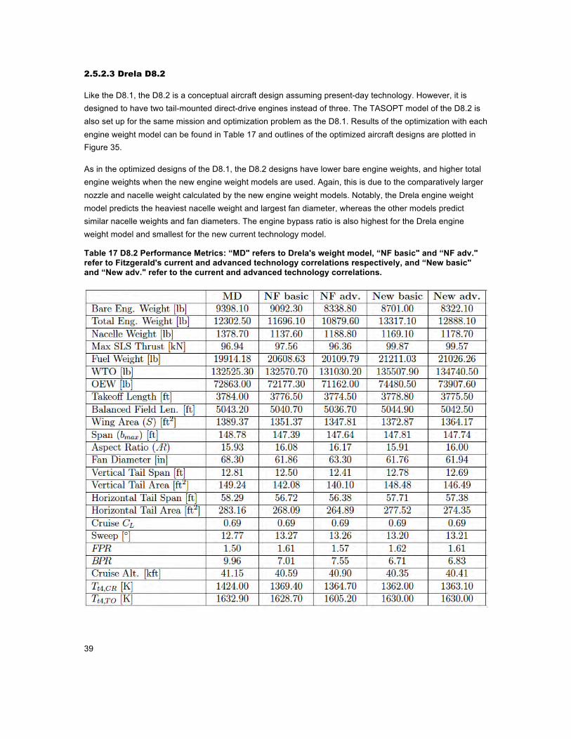
Like the D8.1, the D8.2 is a conceptual aircraft design assuming present-day technology. However, it is designed to have two tail-mounted direct-drive engines instead of three. The TASOPT model of the D8.2 is also set up for the same mission and optimization problem as the D8.1. Results of the optimization with each engine weight model can be found in Table 17 and outlines of the optimized aircraft designs are plotted in Figure 35.

As in the optimized designs of the D8.1, the D8.2 designs have lower bare engine weights, and higher total engine weights when the new engine weight models are used. Again, this is due to the comparatively larger nozzle and nacelle weight calculated by the new engine weight models. Notably, the Drela engine weight model predicts the heaviest nacelle weight and largest fan diameter, whereas the other models predict similar nacelle weights and fan diameters. The engine bypass ratio is also highest for the Drela engine weight model and smallest for the new current technology model.


40



-60

-40

-20

0

20

40

60

80

-80 -60 -40 -20 0 20 40 60 80

[ft]

[ft]

MDNF current


New advanced

41

The engines produce about the same maximum static thrust in each of the optimized designs, and the fuel weight, gross takeoff weight, and OEW are also about the same, though slightly higher in the new models. The optimal takeoff length, balanced field length, wing size and sweep were also not affected by the different weight models.

Plotted in Figure 36 is the TASOPT-predicted fuel burn rate in lbm/s during cruise of the optimized D8.2 for each engine weight model. As with the D8.1, the new models are more conservative than the Drela and Fitzgerald models, with the new current technology model being the least optimistic. Again, this is due to the larger engine weight and OEW, as well as a slightly lower cruise altitude than the other models.

2.5.2.4 Drela D8.5

The D8.5 is a conceptual aircraft design with three tail-mounted geared engines assuming advanced materials technology. The TASOPT model of the D8.5 is also set up for the same mission and optimization problem as the D8.1 and D8.2. Results of the optimization with each engine weight model can be found in Table 18 and the geometry of each design is plotted in Figure 37.

The main difference between the optimized D8.5 designs is the larger variation in wing span and area, which is illustrated in Figure 37. The Fitzgerald current technology model produces the largest wing and tail corresponding to the highest maximum static thrust of all the models, whereas the Fitzgerald advanced technology model produces the smallest wing and tail and lowest static thrust. Consequently, it also has the highest cruise lift coefficient. The new current and advanced technology models actually produce relatively similar-sized aircraft in terms of wing size, static thrust, engine bypass ratio, and fan diameter.

As with the D8.1 and D8.2, takeoff gross weight, OEW, total engine weight and fuel weight is higher for the new engine weight models than the other models. Optimal values for cruise lift coefficient, FPR, wing aspect ratio, and wing sweep are similar across engine weight models, but there are variations in takeoff length and balanced field length. In general, cruise altitude is lower for the advanced technology models, but there is a larger difference in altitudes between the Fitzgerald current and advanced technology models than between the new current and advanced technology models.

42


Plotted in Figure 38 is the TASOPT-predicted fuel burn rate in lbm/s during cruise of the optimized D8.5 for each engine weight model. As with the D8.1 and D8.2, the new models are more conservative than the Drela and Fitzgerald models due to the larger fuel weight required. However, there is no difference in fuel burn rate between the optimized D8.5 with current technology engines and the optimized D8.5 with advanced technology engines. This follows from the similarity in airframe geometry and gross takeoff weight and is an interesting result since we would expect a larger variation in optimal design with advances in engine technology.

43



-60

-40

-20

0

20

40

60

80

-100 -80 -60 -40 -20 0 20 40 60 80 100

[ft]

[ft]

MDNF current


New advanced

44

3 HPC Polytropic Efficiency Correction

3.1 Background

In the current version of TASOPT, the High Pressure Compressor (HPC) polytropic efficiency is input as a constant value. To improve the accuracy of the TASOPT engine model, we add a model that estimates the HPC polytropic efficiency as a function of compressor exit corrected mass flow. In this work, we consider the specific case of small-core engines, defined as those with compressor exit corrected mass flow between 1.5 and 3.0 lbm/s. The efficiency of small-core engines is limited by the effects of low Reynolds number flow and manufacturing limitations, and this effect is modeled by a correction to the HPC polytropic efficiency based on a correlation of published data.

DiOrio quantified polytropic efficiency degradation for compressors with exit corrected mass flow less than 6 lbm/s due to a) low chord Reynolds number, which can be as low as 160,000 for compressor with exit corrected mass flow of 1.5 lbm/s if blades are not optimized for low-Re flow and b) larger non-dimensional tip clearances [5]. The Reynolds number related losses on the rotor blades and stator vanes were analyzed using MISES, a 2D cascade code, and the tip clearances losses were analyzed using CFD computations. Based on the analysis, he developed an estimate for the HPC polytropic efficiency decrease as a function of compressor exit corrected mass flow (𝑚!!") for three compressor configurations: Pure Scale, Shaft Limited, and Shaft Removed. The pure scale configuration is the case in which a modern axial compressor with exit corrected mass flow of 6.0 lbm/s is scaled down geometrically to 1.5 lbm/s. The shaft-limited configuration accounts for the case in which the HPC scaling is constrained by the LP shaft that needs to pass through it, and thus has an increased mean radius and hub-to-tip ratio compared to the pure scale configuration. Lastly, the shaft-removed configurations allows for larger blade heights by eliminating the LP shaft constraint, which is the most ideal configuration. Plots of change in polytropic efficiency (𝛥𝜂!"#$,!"#) with 𝑚!"# are shown in Figure 39 and Figure 40. Case A and Case B represent the estimated upper and lower bounds on compressor efficiency respectively. Case A assumes that blade optimization was used to mitigate Reynolds number effects and that tip clearances scale with compressor radius. Case B assumes that the blades were not optimized and tip clearances are not scalable, i.e. that as the compressor radius shrinks, tip clearance remains constant. The shaft-limited and pure scale curves from these plots form the basis of efficiency correction functions included in the new version of TASOPT.

45

Figure 39 HPC efficiency versus core size for Case A (efficiency upper bound). Baseline efficiency at 6.0 lbm/s. [5]

Figure 40 HPC efficiency versus core size for Case B (efficiency upper bound). Baseline efficiency at 6.0 lbm/s. [5]

46

3.2 Correction Implementation in TASOPT

The HPC polytropic efficiency correction is implemented in TASOPT as a continuous correlation of 𝛥𝜂!"#$,!"# as a function of 𝑚!"#. There are four versions of the correction included, a) Case A, Pure Scale, b) Case A, Shaft Limited, c) Case B, Pure Scale, and d) Case B, Shaft Limited, which the user can select using a flag in the TASOPT input file (including an option to apply no efficiency correction). The correlation function for each version of the correction was approximated by fitting a function of the form

Δ𝜂!"#$,!"# =!

! ! !

!"# ! ! !!!"#!

+ 𝑐 Eq. 7

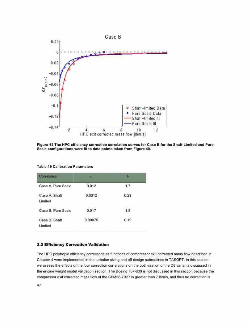
to points from the curves in Figure 39 and Figure 40, where 𝑎, 𝑏, and 𝑐 are fit parameters. With 𝑐 set to -1, this function approaches zero asymptotically. Though the curves may have been better-approximated by piecewise functions, a continuous function form was chosen so that the derivative of the function would also be continuous, allowing the engine sizing subroutines in TASOPT to converge more reliably than if the derivative were discontinuous. The disadvantage of this approach is that, since the function does not go to zero at 6.0 lbm/s, an efficiency correction is applied even for engines with compressor exit corrected mass flow greater than 6.0 lbm/s. To mitigate this issue and move the correlation curve closer to zero, 𝑐 was chosen to be -0.9999 with 𝑎 and 𝑏 remained as fit parameters. The curve fits can be found in Figure 41 and Figure 42, and Table 19 contains the values of the fit parameters for each correlation.

Figure 41 The HPC efficiency correction correlation curves for Case A for the Shaft-Limited and Pure Scale configurations were fit to data points taken from Figure 39.

2 4 6 8 10 12−0.14

−0.12

−0.1

−0.08

−0.06

−0.04

−0.02

0

0.02

H P C ex it co rrected m ass flow [lbm /s]

∆η po

ly,H

C

C ase A

S haft−lim ited D ataP ure S ca le D ataS haft−lim ited fitP ure S ca le fit

47

Figure 42 The HPC efficiency correction correlation curves for Case B for the Shaft-Limited and Pure Scale configurations were fit to data points taken from Figure 40.

Table 19 Calibration Parameters

Correlation 𝑎 𝑏

Case A, Pure Scale 0.012 1.7

Case A, Shaft Limited

0.0012 0.29

Case B, Pure Scale 0.017 1.8

Case B, Shaft Limited

0.00075 0.19

3.3 Efficiency Correction Validation

The HPC polytropic efficiency corrections as functions of compressor exit corrected mass flow described in Chapter 4 were implemented in the turbofan sizing and off-design subroutines in TASOPT. In this section, we assess the effects of the four correction correlations on the optimization of the D8 variants discussed in the engine weight model validation section. The Boeing 737-800 is not discussed in this section because the compressor exit corrected mass flow of the CFM56-7B27 is greater than 7 lbm/s, and thus no correction is

2 4 6 8 10 12−0.14

−0.12

−0.1

−0.08

−0.06

−0.04

−0.02

0

0.02

H P C ex it co rrected m ass flow [lbm /s]

∆η po

ly,H

C

C ase B

S haft−lim ited D ataP ure S ca le D ataS haft−lim ited fitP ure S ca le fit

48

applied by any model. For each of the D8.x aircraft, the “default" engine weight model is used and only the HPC efficiency correction correlation is varied while TASOPT is run in optimization mode.

3.3.1 Problem Setup

As discussed in Chapter 4, Case A is an upper bound estimate on HPC efficiency and Case B is the lower bound. There are two correction correlations for each case: the “pure scale" configuration, which assumes that a modern axial compressor was scaled down, and the “shaft-limited" configuration, which has an increased mean radius and hub-to-tip ratio compared to the pure scale configuration, and is therefore more pessimistic. We expect the Case B shaft-limited correction to have the largest effect on airframe and engine properties and the Case A pure scale correction to have the smallest effect. Harsher efficiency corrections should drive the optimizer to increase the core size of the engine by decreasing the bypass ratio or increasing the overall engine size. We also expect the optimizer to increase the wing area and aspect ratio and decrease thrust to compensate for the decreased engine efficiency.

3.3.2 D8.1

The D8.1 optimization problem was set up in the same way as in section 1.2.2, with a payload of 38,700 lb, range of 3000 nmi, and the Fitzgerald current technology engine weight model. The starting HPC polytropic efficiency is 0.89. Since the propulsion mass flow is split between three engines, the HPC exit corrected mass flow is around 3 lbm/s with no efficiency correction. The efficiency correction at this core size is about -1%.

49

Table 20 D8.1 Performance Metrics

Results of the optimization with each HPC efficiency correction model can be found in Table 20 and the geometry of each design is plotted in Figure 43. As expected, the optimizer compensates by increasing the core size, as evidenced by the larger HPC exit corrected mass flow for the case B corrections compared to the case A corrections, and the shaft-limited corrections compared to the pure scale corrections. By increasing the core size, the optimizer maintains the HPC polytropic efficiency at 0.88. Note that the increasing core size is achieved by increasing the fan diameter and decreasing the bypass ratio. The increased engine size causes engine weight to increase, which in turn, causes OEW, fuel weight, and WTO to increase. The decreased 𝐵𝑃𝑅 causes static thrust to decrease slightly. Wing span and area increase due to the increased takeoff weight and decreased static thrust. Horizontal and vertical tail sizes increase to match the wing. The optimizer also tries to compensate for the decreased engine efficiency by increasing the cruise lift coefficient and altitude and decreasing the engine operating temperature.

50

Figure 43 Comparison of HPC efficiency correction effect on airframe geometry for D8.1

Figure 44 Comparison of HPC efficiency correction effect on fuel burn during cruise for D8.1

-60

-40

-20

0

20

40

60

80

-80 -60 -40 -20 0 20 40 60 80

[ft]

[ft]

No CorrectionCase A, Pure Scale

Case A, Shaft-limitedCase B, Pure Scale

Case B, Shaft-limied

51

Plotted in Figure 44 is the TASOPT-predicted fuel burn rate in lbm/s during cruise of the optimized D8.1 for version of the HPC efficiency correction model. As expected, the lowest fuel burn rate is the aircraft optimized with no efficiency correction, and the Case A pure scale correction has a lower fuel burn rate than the shaft limited correction. Note that the fuel burn rate is nearly identical for both Case B correction functions.

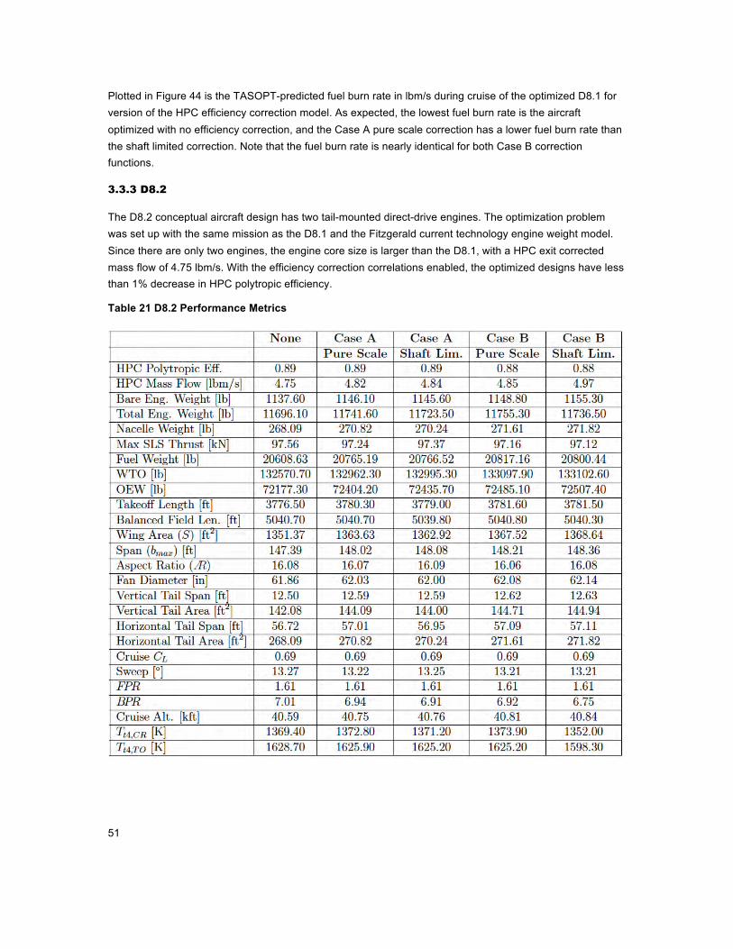
3.3.3 D8.2

The D8.2 conceptual aircraft design has two tail-mounted direct-drive engines. The optimization problem was set up with the same mission as the D8.1 and the Fitzgerald current technology engine weight model. Since there are only two engines, the engine core size is larger than the D8.1, with a HPC exit corrected mass flow of 4.75 lbm/s. With the efficiency correction correlations enabled, the optimized designs have less than 1% decrease in HPC polytropic efficiency.


52



-60

-40

-20

0

20

40

60

80

-80 -60 -40 -20 0 20 40 60 80

[ft]

[ft]

No CorrectionCase A, Pure Scale

Case A, Shaft-limitedCase B, Pure Scale

Case B, Shaft-limied

53

Results of the optimization with each HPC efficiency correction model can be found in Table 21. Comparing the geometry plot in Figure 45 for the D8.2 with Figure 43, it is clear that the airframe changes due to the HPC efficiency correction are less drastic than those observed for the D8.1. As with the D8.1, the optimizer increases engine core size to compensate for the efficiency correction by decreasing the bypass ratio and increasing the fan diameter. As a result, engine weight, OEW, fuel weight, and takeoff weight increase. Thrust decreases slightly with the decreased bypass ratio and wing and tail sizes increase. Cruise lift coefficient and wing sweep stay relatively constant, while cruise altitude increases slightly.

Plotted in Figure 46 is the TASOPT-predicted fuel burn rate in lbm/s during cruise of the optimized D8.2 for version of the HPC efficiency correction model. In this case, there is almost no difference between the fuel burn rates for different versions of the efficiency correction. Any HPC efficiency correction increases the fuel burn rate compared to no correction, as expected.

3.3.4 D8.5

The D8.5 conceptual aircraft design has three tail-mounted geared engines and assumes advanced technologies. The optimization problem was set up in the same way as for the D8.1 and D8.2 with the Fitzgerald advanced technology engine weight model. The D8.5 is designed with a higher 𝐵𝑃𝑅 engine compared to the D8.1, so the core is even smaller with an HPC exit corrected mass flow of 0.85 lbm/s. With the pure scale corrections, this core size leads to a 3-4% decrease in HPC polytropic efficiency. TASOPT does not converge with the shaft-limited corrections because the efficiency decrease is too large. Results of the optimization with the Case A and Case B pure scale efficiency correction models can be found in Table 22.

54


From the airframe geometries plotted in Figure 47 we can see that both efficiency corrections result in a dramatically larger wing compared to the optimized design with no efficiency correction. The Case B wing is slightly larger than Case A. In the table, there is little difference between the Case A and Case B optimized designs, and the trends of how the output parameters change with the efficiency correction do not necessarily follow those of the D8.1 and D8.2. The engine size and fan diameter do increase while the bypass ratio decreases to grow the core size. However, unlike in the D8.1 and D8.2 the maximum static thrust increases in the D8.5. Engine weight, OEW, and fuel weight increase as expected, but takeoff distance decreases due to the much larger wing and available static thrust. We also see the cruise lift coefficient decrease and the wing sweep increase with a 4000 ft increase in cruise altitude. In the engine, the fan pressure ratio increases slightly while the operating temperature remains relatively constant.

55



-60

-40

-20

0

20

40

60

80

-100 -80 -60 -40 -20 0 20 40 60 80 100

[ft]

[ft]

No CorrectionCase A, Pure ScaleCase B, Pure Scale

56

The fuel burn rate during cruise in lbm/s for each D8.5 design is plotted in Figure 48. There is only a small difference in fuel burn rate between the designs with the HPC efficiency correction and the one with no correction, despite the major differences in the airframe and engine designs. This is because the optimizer has chosen the design to minimize fuel burn.

4 Conclusion

As part of the effort to perform system-level UQ of the TASOPT-AEDT coupled system, the main objective of this work was to improve the accuracy and expand the applicability of TASOPT. This was accomplished by developing a more accurate engine weight model, and by modifying the thermodynamic cycle model to include turbomachinery size effects on efficiency. These tasks were achieved by building separate engine component weight models using data from WATE++ and state-of-the-art regression techniques and combined them to estimate total engine weight, and by implementing a correction to compressor efficiency based on a function of compressor exit corrected mass flow. These additions allow TASOPT to better estimate the performance of aircraft designs featuring high bypass ratio and advanced technology propulsion systems.

The new engine weight model has been applied in TASOPT to four case studies. In the case of the TASOPT model of the Boeing 737-800, TASOPT sized an aircraft that performs most similarly to the actual 737-800 with the new current technology engine weight model than with the previously existing engine weight models. Next, the effect of the new engine model on the optimization of three D8.x variants was explored. For baseline technology variants with direct-drive engines (the D8.1 and D8.2), the new engine weight model leads to heavier engine assemblies and more conservative fuel burn estimations, but very little difference in airframe geometry compared to the other engine weight models. Optimization of the D8.5, an advanced technology design with geared high bypass ratio engines, is more sensitive to choice of engine weight model, with larger variations in wing span and structural weight observed. These results illustrate that the new engine weight model accurately estimates engine weight and leads to better aircraft geometry and performance estimates.

The HPC polytropic efficiency correction models were applied to the three D8.x cases. As expected, the decreased compressor efficiency drove the optimizer to increase the core size and overall engine size to reduce the effect of the correction in all three cases. The efficiency correction had a greater effect on the 3-engine configuration of D8.1 than on the 2-engine configuration of the D8.2 due to the smaller core mass flow, illustrating the trade-off between a 2-engine and 3-engine configuration. The D8.5, an extremely high bypass ratio 3-engine configuration, has the smallest core mass flow of the three cases. Under optimization, the HPC efficiency correction caused a significant increase in wing area and decrease in BPR for the D8.5. These results illustrate that the HPC polytropic efficiency correction improves TASOPT's ability to accurately model small-core engines.

57

References

[1] Drela, M., “Simultaneous Optimization of the Airframe, Powerplant, and Operation of Transport Aircraft," Tech. rep., MIT Department of Aeronautics and Astronautics, 2010.

[2] Kerrebrock, J., Aircraft Engines and Gas Turbines, 2nd Ed., The MIT Press, Cambridge, MA, 1996.

[3] Onat, E. and Klees, W., “A method to estimate weight and dimensions of large and small gas turbine engines," Tech. Rep. CR-159481, NASA, January 1979.

[4] Jones, S., “An Introduction to Thermodynamic Performance Analysis of Aircraft Gas Turbine Engine cycles Using the Numerical Propulsion System Simulation Code," Tech. Rep. TM-2007-214690, NASA Glenn Research Center, Cleveland, OH, 2007.

[5] DiOrio, A., Small Core Axial Compressors for High Efficiency Jet Aircraft, Master's project, Massachusetts Institute of Technology, Dept. of Aeronautics and Astronautics, Sept. 2012.

[6] Greitzer, E. M., Bonnefoy, P., la Rosa Blanco, E. D., C. Dorbian, M. D., Hansman, R. J., Hileman, J., Liebeck, R. H., et al., “N+3 Aircraft Concept Designs and Trade Studies, Final Report," NASA Grant/Cooperative Agreement NNX08AW63A, NASA, 2010.

[7] Saltelli, A., Ratto, M., Andres, T., Campolongo, F., Cariboni, J., Gatelli, D., Saisana, M., and Tarantola, S., Global Sensitivity Analysis: The Primer, chap. 4, John Wiley & Sons Ltd., West Sussex, England, 2008, pp. 164-167.

[8] Sobol', I., “Sensitivity analysis for non-linear mathematical models," Mathematical Modeling & Computational Experiment (Engl. Transl.), Vol. 1, 1993, pp. 407-414.

[9] Rasmussen, C. and Williams, C., Gaussian Processes for Machine Learning, Vol. 14, MIT Press, 2006.

[10] Daly, M., IHS Jane's Aero Engines, IHS Global Inc., 2009.

[11] Drela, M., “Turbofan Weight Model from Historical Data," 2009.

[12] Drela, M., “Development of the D8 Transport Configuration," 29th Applied Aerodynamics Conference, AIAA Paper 2011-3970.

[13] “737 Airplane Characteristics for Airport Planning," Tech. rep., The Boeing Company, September 2013.

[14] Beltramo, M. N., Trapp, D. L., Kimoto, B. W., and Marsh, D. P., “Parametric study of transport aircraft systems cost and weight," Technical Report CR-151970, NASA, April 1977.

58

Appendix A

Surrogate Model Equations

This appendix contains explicit equations for the least squares models for each configuration. GP models cannot be expressed as explicit equations, but require several hundred training points for prediction, so they have been excluded.

A.1 Direct Drive, Current Technology

59

A.2 Direct Drive, Advanced Technology

61

A.3 Geared, Current Technology

62

A.4 Geared, Advanced Technology

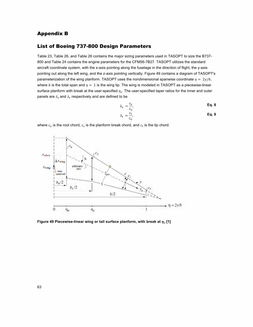
63

Appendix B

List of Boeing 737-800 Design Parameters

Table 23, Table 26, and Table 26 contains the major sizing parameters used in TASOPT to size the B737-800 and Table 24 contains the engine parameters for the CFM56-7B27. TASOPT utilizes the standard aircraft coordinate system, with the x-axis pointing along the fuselage in the direction of flight, the y-axis pointing out along the left wing, and the z-axis pointing vertically. Figure 49 contains a diagram of TASOPT's parameterization of the wing planform. TASOPT uses the nondimensional spanwise coordinate 𝜂 = 2𝑦/𝑏, where 𝑏 is the total span and 𝜂 = 1 is the wing tip. The wing is modeled in TASOPT as a piecewise-linear surface planform with break at the user-specified 𝜂!. The user-specified taper ratios for the inner and outer panels are 𝜆! and 𝜆! respectively and are defined to be

λ! =c!c!, Eq. 8

λ! =c!c!, Eq. 9

where 𝑐! is the root chord, 𝑐! is the planform break chord, and 𝑐! is the tip chord.

Figure 49 Piecewise-linear wing or tail surface planform, with break at 𝜼𝒔 [1]

64

Table 23 737-800 Mission Parameters for TASOPT input file

Mission

Range 3000 nmi

Payload 38,700 lb

Cruise start altitude 33,500 ft

Cruise Lift Coefficient

0.55

Cruise Mach number 0.8

Table 24 737-800 Engine Parameters for TASOPT input file

Engine Properties (CFM56-7B27

Metal temperature 1200K

𝑇!!,!" 1500K

𝑇!!,!" 1345K

OPR 30.0

HPC pressure ratio 12.0

FPR 1.65

𝜂!"#$,!"# 0.91

𝜂!"#$,!"# 0.90

𝜂!"#$,!"# 0.89

𝜂!"#$,!"# 0.90

𝜂!"#$,!"# 0.90

BPR 5.1

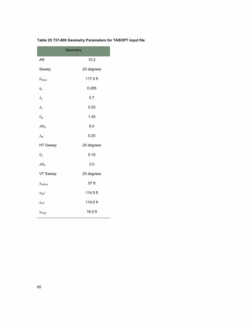
65

Table 25 737-800 Geometry Parameters for TASOPT input file

Geometry

AR 10.2

Sweep 25 degrees

𝑏!"# 117.5 ft

𝜂! 0.285

𝜆! 0.7

𝜆! 0.25

𝑉! 1.45

𝐴𝑅! 6.0

𝜆! 0.25

HT Sweep 25 degrees

𝑉! 0.10

𝐴𝑅! 2.0

VT Sweep 25 degrees

𝑥!"#$ 57 ft

𝑥!" 114.5 ft

𝑥!" 110.0 ft

𝑦!"# 16.0 ft

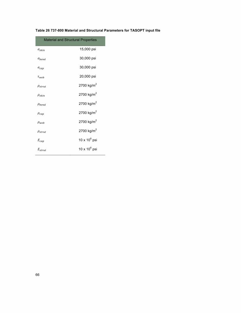
66

Table 26 737-800 Material and Structural Parameters for TASOPT input file

Material and Structural Properties

𝜎!"#$ 15,000 psi

𝜎!"#$ 30,000 psi

𝜎!"# 30,000 psi

𝜏!"# 20,000 psi

𝜌!"#$" 2700 kg/m2

𝜌!"#$ 2700 kg/m2

𝜌!"#$ 2700 kg/m2

𝜌!"# 2700 kg/m2

𝜌!"# 2700 kg/m2

𝜌!"#$" 2700 kg/m2

𝐸!"# 10 x 106 psi

𝐸!"#$" 10 x 106 psi

tasopt engine model developmentpartner.mit.edu/sites/partner.mit.edu/files/report/file/... ·...

Documents