task 8: analysis of freight rail electrification in the scag region
TRANSCRIPT

Task 8.3: Analysis of Freight Rail Electrification in the SCAG Region
Comprehensive Regional Goods Movement Plan and Implementation Strategy

Task 8: Analysis of Freight Rail Electrification in the SCAG Region
Cambridge Systematics, Inc. 8114-008
final technical memorandum
Task 8.3: Analysis of Freight Rail Electrification in the SCAG Region
prepared for
Southern California Association of Governments
prepared by
Cambridge Systematics, Inc. 555 12th Street, Suite 1600 Oakland, CA 94607
date
April 2012


Task 8: Analysis of Freight Rail Electrification in the SCAG Region
Cambridge Systematics, Inc. 8114-008
Table of Contents
1.0 Introduction ................................................................................................. 1-1
1.1 Overview.............................................................................................. 1-1
1.2 Purpose ................................................................................................ 1-1
1.3 Structure of the Memorandum ............................................................ 1-2
2.0 Technology Alternatives Overview............................................................ 2-1
2.1 Alternative #1: Straight-Electric Locomotives (Catenary) .................. 2-1
2.2 Alternative #2: Dual-Mode Locomotives (Electrified Catenary)........ 2-5
2.3 Alternative #3: Linear Synchronous Motor (LSM) System ................ 2-8
2.4 Additional Technologies for Future Consideration............................. 2-9
3.0 Electrification Options and Timeline Overview ....................................... 3-1
3.1 Alameda Corridor (Option I) ............................................................... 3-2
3.2 Ports to West Colton/San Bernardino (Option II) ............................... 3-3
3.3 Ports to Barstow/Indio/Chatsworth/San Fernando (Option III) ....... 3-5
4.0 Evaluation of Electrification Alternatives.................................................. 4-1
4.1 Technology Readiness.......................................................................... 4-1
4.2 Railroad Operations Impacts ............................................................... 4-5
4.3 Total Capital Cost .............................................................................. 4-11
4.4 Operations and Maintenance (O&M) Cost Impacts .......................... 4-13
4.5 Energy Costs Impacts......................................................................... 4-14
4.6 Comparing Discounted Energy Benefits/Costs with Discounted
Capital Costs for the Straight-Electric Alternative, Option III .......... 4-21
4.7 Emissions Impacts.............................................................................. 4-23
4.8 Summary ............................................................................................ 4-28
5.0 Conclusion ................................................................................................... 5-1
A. Locomotive Count Calculation .................................................................. A-1
B. Calculation of Capital Costs ...................................................................... B-1
B.1 Cost of Rail Electrification System: Determining 2011 Baseline
Cost ..................................................................................................... B-1
B.2 Electrification System Cost per Track-Mile (Excluding
Locomotives) ....................................................................................... B-2
B.3 Total Electrification System Cost (Excluding Locomotives) ............... B-3
C. Energy Needs to Power Electrification System......................................... C-1
D. Calculation of Emissions Impacts .............................................................D-1


Task 8: Analysis of Freight Rail Electrification in the SCAG Region
1-1
List of Tables
Table 3.1 Option I Project Timeline................................................................... 3-3
Table 3.2 Option II Project Timeline ................................................................. 3-4
Table 3.3 Option III Project Timeline ................................................................ 3-6
Table 4.1 Technology Readiness of Electrification Technology Options Under Review .................................................................................... 4-2
Table 4.2 Railroad Operations Impact per Technology/Geographic
Electrification Options ....................................................................... 4-7
Table 4.3 Capital Cost Overview .................................................................... 4-12
Table 4.4 Break-Even Electricity Prices ($/kWh, $2010) for High/Low Diesel Cost Scenarios ....................................................................... 4-18
Table 4.5 Energy Cost Savings/(Losses) of Electrified Rail System
Compared to Diesel System, by Option, Billions of Dollars, First Year of Electrification to 2050 .................................................. 4-20
Table 4.6 Percent of Discounted Capital Cost Covered by Savings in
Discounted Energy Costs, 0-, 3-, and 7-Percent Discount Rates, 2012 to 2050a..................................................................................... 4-22
Table 4.7 Diesel Emissions Baseline, SCAB, and Electrification Options I to
III ...................................................................................................... 4-24
Table 4.8 Emissions Reduction through Electrification of Line-Haul
Freight Locomotives: Assuming Zero Off-Site Emissions in the
SCABa............................................................................................... 4-26
Table 4.9 Emissions Reduction through Electrification of Line-Haul
Freight Locomotives: Assuming 30 Percent of Electrification
Power Produced in the SCAB by Natural Gas-Fired Generatorsa ...................................................................................... 4-26
Table 4.10 Emissions Reduction through Electrification of Line-Haul
Freight Locomotives: Off-site Emissions Outside of the SCAB Incorporateda ................................................................................... 4-27
Table 4.11 Percent Emissions Reduction as a Result of Option III
Electrification, 2035a,b....................................................................... 4-27
Table A.1 Locomotives per Train, Baseline ...................................................... A-3
Table A.2 Diesel Locomotive Counts................................................................ A-4
Table A.3 Electric Locomotive Counts.............................................................. A-4

Task 8: Analysis of Freight Rail Electrification in the SCAG Region
1-2
Table B.1 Electrification System Cost per Track-Mile – 2011 Dollars,
Undiscounted, Excluding Locomotive Costsa .................................. B-2
Table B.2 Electrification System Track-Miles ................................................... B-3
Table B.3 Cost per Locomotive Unit ................................................................ B-4
Table B.4 Total Locomotive Cost Through 2035 (Undiscounted) .................... B-5
Table C.1 Projected Railroad Diesel Prices (2010 Cents per Gallon)a ............... C-2
Table C.2 Projected Price of Electricity for Southern California Edison
(2010 Cents per kWh) ....................................................................... C-3
Table C.3 Option III Straight-Electric/Dual-Mode Technology, Line-Haul Locomotive Break-Even Energy Price Analysis ............................... C-7
Table D.1 Key Factors Utilized to Calculate Emissions from Electrification.... D-1
Table D.2 CO2 Daily Emissions per Electrification Option – Various
Scenarios ........................................................................................... D-2
Table D.3 PM2.5 Daily Emissions per Electrification Option – Various Scenarios ........................................................................................... D-2
Table D.4 NOx Daily Emissions per Electrification Option – Various Scenarios ........................................................................................... D-3

Task 8: Analysis of Freight Rail Electrification in the SCAG Region
1-1
List of Figures
Figure 2.1 Freight Railroad Powered by Electrified Catenary ........................... 2-2
Figure 2.2 Typical Configuration of an Electrified System ................................ 2-3
Figure 2.3 Linear Motor Overview ..................................................................... 2-8
Figure 3.1 Summary of Regional Electrification Options Analyzed .................. 3-2
Figure 4.1 NASA Technology Readiness Scale .................................................. 4-2
Figure 4.2 Average Annual World Oil Prices in Three Cases, 1980 to 2035..... 4-15
Figure 4.3 Regional Electrification Options and the SCAB Boundary ............. 4-24
Figure 4.4 Evaluation of Electrification Alternatives through Key Evaluation Criteria .......................................................................... 4-30


Task 8: Analysis of Freight Rail Electrification in the SCAG Region
1-1
1.0 Introduction
1.1 OVERVIEW Electrification of key mainline railroad corridors in the Southern California
region is one strategy that can reduce emissions from the freight transportation
sector, and would move the region closer to regional air quality attainment requirements. Electrified rail is a proven technology used throughout the world
for both passenger and freight rail purposes. However, there are a number of
issues that make implementation of rail electrification in Southern California a
challenging proposition for the railroads and the public sector, including high upfront capital costs, impacts on operations, and long-term energy cost and
availability. This memorandum furthers the discussion concerning the benefits
and drawbacks of rail electrification options.
This analysis builds on and updates previous rail electrification work completed
for the 2008 SCAG Regional Transportation Plan. In the 2008 document, capital costs and project timelines were estimated, among other items. In this
memorandum, potential alternative locomotive and electrification technologies,
technology readiness of key electrification technologies, capital costs, emissions
reductions, railroad operational impacts, and potential longer-term railroad
energy cost savings as a result of electrification are estimated. In a separate report being prepared for the SCAG Goods Movement Study, electrification will
be compared to the accelerated Tier IV technology rail emissions reduction
strategy in terms of cost effectiveness and emissions reduction. This
memorandum will also identify opportunities for near- and mid-term initiatives, as well as create a framework for consideration of long-term initiatives.
Representatives from California Environmental Associates (CEA – working with
the Class I railroads in the region), the South Coast Air Quality Management
District (AQMD), and the California Air Resources Board (ARB) all provided
important input into the assumptions and information presented in this analysis. Several working group meetings were held to discuss key assumptions, opera-
tional considerations, and other topics that relate to freight rail electrification.
1.2 PURPOSE It is important to note that the purpose of this analysis is not to definitively state
whether electrification of the rail system in the SCAG region is cost effective or
not. There are numerous areas within the report that require further analysis and research to come to a more precise conclusion regarding the cost effective-
ness of rail electrification. This report, however, does look at worst and best case

Task 8: Analysis of Freight Rail Electrification in the SCAG Region
1-2
scenarios that will allow decision-makers to better understand key benefits and
drawbacks of potential zero local emissions rail technologies for the region. This
report will also help determine key data gaps and where further analysis or RD&D is required to come to a better understanding of key benefits (emissions
reductions and potential energy cost savings) and drawbacks (such as costs and
operations concerns) of electrification technologies. It is also important to note
that, given the status of technology appropriate to U.S. freight operations and the status of any planning for what would be an operationally challenging system
transformation (integrating a partially electrified system in Southern California
with a national system that is not electrified), it is unlikely that electrification of
major freight routes could be completed in time to meet the 2023 South Coast Air
Basin (SCAB) deadline for the eight-hour ozone National Ambient Air Quality Standards (NAAQS). However, the region must attain stringent ozone standards
by 2031; and as a result, rail electrification and other zero local emissions tech-
nologies are relevant beyond 2023. If implemented, an emissions reduction
strategy such as electrification should be seen as a long-term strategy, not as one
to meet near- to medium-term emissions targets.
1.3 STRUCTURE OF THE MEMORANDUM This report is organized into the following sections:
1. Technology alternatives overview. This section describes the three key elec-
trification technologies analyzed in this study (straight-electric (catenary);
dual-mode (catenary); and a linear synchronous motor (LSM) system). An
overview of each technology is provided, and key benefits and drawbacks discussed.
2. Electrification Options and Timeline Overview. This section highlights the
three geographic options under consideration.
3. Evaluation of electrification alternatives. The three technology alternatives
and each geographic option within each alternative are evaluated based on technology readiness, railroad operations impacts, total capital cost, energy
cost savings and SCAB region total emissions reduction. In addition,
discounted energy costs/benefits are compared against estimated discounted
capital costs for one electrification option.
4. Conclusion. This section provides a brief summary of results and key con-
clusions, and suggests steps to be taken for further analyses.

Task 8: Analysis of Freight Rail Electrification in the SCAG Region
2-1
2.0 Technology Alternatives Overview
As highlighted in the SCAG Goods Movement Study Task 8.1, “Technology Overview” report, a host of zero or near-zero emission technology options are
available as potential options to move goods from the Ports of Long Beach and
Los Angeles to inland destinations in order to help the region meet air quality
attainment standards. For the purposes of this report, three of the most promi-nent electrification options available for railroad applications are evaluated. These
options include straight-electric locomotives (catenary), dual-mode locomotives
(catenary), and electric (linear synchronous). Note that the technologies under
review in this technical memorandum focus on rail electrification technologies
that can effectively utilize existing track infrastructure and right-of-way. The purpose of this section is to present an overview of each of the three technolo-
gies, and to highlight some of their known constraints. Additional technologies
that do not use electrification are briefly discussed at the conclusion of this
section but are not fully analyzed in this report.
2.1 ALTERNATIVE #1: STRAIGHT-ELECTRIC
LOCOMOTIVES (CATENARY) This technology alternative requires the transmission of electricity from power
generation plants to straight-electric locomotives via overhead wires (also known as catenaries). It differentiates itself from the other options in that it: 1) relies
solely on catenaries for electricity, and 2) relies on a straight-electric locomotive
to move freight trains. The use of catenaries to power freight trains has been
proven throughout the world, and is the most common way to electrify freight
and passenger railroads. In addition, the straight-electric locomotive is the most common type of locomotive used to pull freight and passenger trains that oper-
ate electrically. Figure 2.1 below shows a state-of-the-art, heavy-haul LKAB iron
ore freight train in Torneträsk, Sweden, being powered by catenaries.
In order to make the move from a system that relies on diesel locomotives (cur-rent scenario) to a straight-electric system with electrified catenary, the purchase
of new straight-electric locomotives would be required. In addition, the con-
struction of an overhead line system that aligns with current tracks and is com-
patible with the height requirements of double-stack trains currently moving in
the L.A. region is also necessary. The construction of an electric system in terms of labor, timeline, and cost for the SCAG region, is discussed further in subse-
quent sections of this report.

Task 8: Analysis of Freight Rail Electrification in the SCAG Region
2-2
Figure 2.1 Freight Railroad Powered by Electrified Catenary
Source: David Gubler, 22.3.2011 (http://bahnbilder.ch/picture/7743?title=iore).
Straight-Electric Power System Design
Figure 2.2 below highlights a typical configuration of an electrified rail system.
Power supply substations are located along the electrified system route. These
substations then supply power to a single-phase overhead distribution system.1 Modern electric railroads operate primarily at a standard nominal electrification
voltage of 25kV, while some operate at 50kV. The cost effectiveness of one
option versus the other depends on a variety of factors, such as the number of
low-clearance bridges/tunnels on the electrified route (25kV requires lower
clearances). The 50kV systems, on the other hand, require fewer substations, which can result in savings in the capital cost of the power system. For more
detail on the pros and cons of each of these options, please review the GO
Electrification Study or the 1992 SCRRA Southern California Accelerated
Electrification Program Report, Volume 2.
1 Southern California Accelerated Rail Electrification Program Report, prepared for the Southern California Regional Rail Authority (SCRRA), 1992.

Task 8: Analysis of Freight Rail Electrification in the SCAG Region
2-3
Figure 2.2 Typical Configuration of an Electrified System
Source: Southern California Accelerated Rail Electrification Program Report, prepared for the SCRRA, 1992.
In addition to the selection of system voltage, other components of the system
must also be determined, such as the power distribution types (for example, simple catenary system, twin contact wire system, or single contact wire system).
Cantilever structures and portal and headspan structures must also be selected.
The configuration of the electrification system is outside the scope of this analy-
sis, but must be considered again in detail before moving forward.

Task 8: Analysis of Freight Rail Electrification in the SCAG Region
2-4
Straight-Electric Freight Locomotives in Use
Several straight-electric locomotives are in use for freight operations throughout
the world, which could be adapted for use in United States freight operations.
At present, there are only a handful of straight-electric freight locomotives in use in the United States, of which all were built 30 or more years ago. Several exam-
ples of current generation heavy-haul straight-electric freight locomotives are
highlighted below.2
1. The Swedish mining company LKAB operates 26 IORE full electric locomo-
tives built by Adtranz and its successor Bombardier Transportation in Germany.3 Comprised of two sections permanently connected by a drawbar,
these are the most powerful freight locomotives in production in the world,
with each section producing a total continuous output of 5,400 kW (7,200 hp
total). The starting tractive effort is approximately 600 kN. Locomotives
based on this platform are in use throughout Europe, and a derivative adapted to U.S. requirements has been imported by New Jersey Transit.
These units follow European UIC standards; however, the IORE units are
similar to American design, especially in their use of Association of American
Railroads (AAR) couplers, loading gauge, and axle loading specifications.
2. Queensland Rail is operating Siemens 3800 model electric locomotives to
transport coal for export. The locomotives can operate both on 25 kV and
50 kV systems, and have a starting tractive effort of 525 kN, and power out-
put of nearly 5,400 hp.4
3. South African Railways (SAR) has deployed straight-electric locomotives (Mitsui Class 15E locomotive, with specifications of 6,000 hp, 580 kN starting
tractive effort, 50 kV) on the 535-mile long Sishen-Saldanha iron-ore railway.5
Currently, 76 locomotive units are deployed for this service, and
32 additional units are on order. Additionally, SAR follows AAR standards, so this technology is directly applicable to North American freight movement.
2 An obvious alternative that is not discussed here would be the adaptation of one or more of the common North American heavy-haul diesel designs to straight electric operation. While this is clearly possible, and was done in the past by both of the large OEM locomotive manufacturers General Electric and EMD (now part of Caterpillar), neither have produced electric locomotives in more than 25 years. Nevertheless, industry experts believe that both EMD and GE, and particularly the latter, could bring to market an electric locomotive that is based on their proven current diesel designs.
3 Bombardier: http://www.webcitation.org/5tkALuPQ7.
4 http://www.schmalspur-europa.at/schmal_QR%203800%20Schmalspurlokomotive.pdf.
5 Transnet press release from March 2, 2011, http://commons.wikimedia.org/w/index.php?title=File%3ATRANSNET_BUYS_32_MORE_LOCOMOTIVES_FROM_MITSUI.pdf&page=1.

Task 8: Analysis of Freight Rail Electrification in the SCAG Region
2-5
4. Indian Railways (IR) utilizes a variety of heavy-haul locomotives, the most
modern one being the WAG 9, produced by ABB and Chittranjan Locomotive
Works (CLW). Two of these units can haul 4,500-ton trains on gradients of 1:60. The continuous power at the wheels is 6,000 hp. In terms of railway
standards, IR has a mixture of British and U.S. standards, and a considerable
volume of their freight traffic is categorized as heavy haul.
A variety of other high horsepower electric freight locomotives is in operation in Europe, such as the DB Schenker EG3100 (8,837 hp), or the Bombardier Swiss
Class 482 Traxx Locomotive (7,614 hp). However, in their present configura-
tions, these units do not offer sufficient starting tractive effort to move typical
high-tonnage trains up the critical mountain passes that must be crossed to enter
or leave the L.A. region (i.e., the Cajon Pass on BNSF/UP and Beaumont Hill on the UP).
For purposes of this analysis, the assumed locomotive type will be one with sim-
ilar specifications to the Bombardier IORE, due to its relatively high tractive
effort (which is necessary to get long and heavy U.S. freight trains moving), six-
axle design, high horsepower, and its potential adaptability to the U.S. freight railroad operating environment. While some adjustments would be necessary to
prepare these locomotives for U.S. operations (such as additional weight to
increase tractive effort), they should be relatively minor.
2.2 ALTERNATIVE #2: DUAL-MODE LOCOMOTIVES
(ELECTRIFIED CATENARY) This alternative relies on the transmission of electricity from power generation
plants to dual-mode locomotives via electrified catenary, similar to Alternative #1.
It differentiates itself from the other three options, in that it 1) relies on electrified catenary for the transmission of electricity, but can also operate on diesel alone
when no electrified catenary exists; and 2) relies on dual-mode locomotives to
move freight trains. Dual-mode locomotives are more flexible than straight-
electric locomotives with respect to energy source since they can operate using both electric current and diesel-powered engines.
This concept has potential in freight operations, especially if an electrified system
is constructed incrementally across the U.S. In a long-term scenario, dual-mode
locomotives could be used interchangeably in the railroad network, as they could
run primarily on electric power in the SCAG region and in other urban areas with overhead line infrastructure, while running on diesel in areas where electri-
fied catenary has not been constructed. In addition, a fleet of dual-mode loco-
motives would alleviate the major operational concerns of straight-electric
locomotives, which is the need to swap out units between diesel and electric
operation at the “edge” of the electrified system (i.e., West Colton, Barstow, or Indio, depending on the phases discussed later in this report); and the associated
requirement to manage a captive pool of locomotives dedicated to this operation.

Task 8: Analysis of Freight Rail Electrification in the SCAG Region
2-6
However, it would require substantial investment in locomotives and a substan-
tial length of time until enough dual-mode locomotives exist to avoid the issue of
switching locomotives at the edge of an electrified system.
Dual-Mode Locomotive Power System Design
The power system considerations are equivalent to what was described in
Alternative #1.
Dual-Mode Locomotive Examples
Dual-mode locomotives take two forms: symmetric and asymmetric. Symmetric
drive systems offer similar tractive power in both electric and diesel modes,
while asymmetric produce high power in one mode and low in the other. Thus
far, the most common and technically simple arrangement has been asymmetric, with high-power diesel and low-power electric operation. The converse
arrangement, high-power electric operation (utilizing high-voltage AC) and low-
power diesel, is technically more complex and has been produced in modest
quantities for freight and passenger applications.6 Symmetric output dual-mode locomotives exist in small quantities for passenger applications, having been
deployed in the United States (New Jersey Transit), France, Germany, and
Canada. Commercial interest in both types of dual-mode locomotives has grown
substantially in recent years, and many of the major locomotive manufacturers
are developing new designs for both freight and passenger use.
For main line freight operations of the type envisioned under this scenario for
Southern California, symmetric design will be necessary. Nevertheless, exam-
ples of both asymmetric and symmetric dual-mode freight locomotives, along
with the New Jersey Transit passenger locomotive, are described below. The
6 Dual-mode locomotives that perform at high-power levels in diesel, while also being able to use low-voltage DC (1,500 volts or less) third-rail or catenary for low to medium-power electric operations, have existed for years in both passenger and freight operations in the U.S. and elsewhere. (Recent U.S. examples include the GE P32AC-DM that are operated by Amtrak and Metro North.) However, dual-power locomotives that produce high-tractive power output in both modes, while utilizing high-voltage AC for electric operations, have only become technically feasible in recent years. Advances in solid state power electronics and compact high-voltage switch gear and transformers have reduced volume and weight requirements to a level where they can be fitted into a locomotive car body together with all of the equipment required for diesel operation. Even with these advances, current dual-power locomotive designs are at the edge of meeting typical allowable size and weight limits.
AC dual-mode locomotives are technically the most complex and costly, as they require a transformer and associated switch gear, equipment that is unnecessary for high-power, dual-mode DC locomotives. Beyond that, they are largely similar technically to high-power DC locomotives, which typically utilize a 3KV catenary system.

Task 8: Analysis of Freight Rail Electrification in the SCAG Region
2-7
three freight locomotives, some of which utilize AC and others DC electricity
from high-voltage catenary, can be found in South Africa, Spain, and Switzerland.
A modern high-capacity 12.5/25 kV AC dual-mode passenger locomotive is the Bombardier ALP-45DP, which has recently entered service on New Jersey
Transit and Montreal’s Agence Métropolitaine de Transport.7 In electric
operation, the unit develops 4,000 kW (over 5,300 hp) for traction and 316 kN
of starting tractive effort, while in diesel operation performance is reduced to 3,134 kW (4,202 hp). With some redesign, this model could conceivably be
adapted for North American freight use. The required changes include
implementing a six-axle, instead of four-axle wheel arrangement, modifying
the gearing to lower top speed, increasing weight to boost tractive effort, and omitting passenger-related features such as the head-end power systems.
In South Africa, Transnet operates 50 Siemens Class 38-000 3kV DC dual-
mode freight locomotives, the largest dual-mode freight fleet in the world.
Acquired between 1992 and 1994, the performance of these units is asymme-tric, producing 1,500kW in electric and 600 kW in diesel mode, which is
acceptable as the diesel function is only intended for use in “last-mile” switching operations off of electrified main lines. The units have a top speed
of 62 mph, and produce 260 kN starting tractive effort.
The Spanish rolling stock manufacturer CAF released the Bitrac CC 3600 dual-mode locomotive in 2009. The initial version, which has been delivered
to industrial customer Fesur, is intended for use on the Spanish broad-gauge
network under 3 kV DC. In this configuration, they produce 450 kN of starting tractive effort over six axles, 2,900 kW at the wheel under diesel
operation, and 4,450 kW in electric operation. CAF has announced, but not
delivered, a unit that uses high-voltage AC for electric operation. However,
in concept and technology, this unit shares some similarities with the
Bombardier ALP 46-DP.8
Switzerland’s SBB Cargo currently has an order underway for 30 Stadler
Eem 923 dual-mode locomotives. Intended for switching and light freight
duties, these two-axle units will develop a modest 1,500 kW tractive output
under 15 kV/25 kV electric operation, and only 290 kW with diesel.9
In general, the dual-mode locomotive that most closely matches the needs for
U.S. freight operations is the Bombardier ALP-45DP, as it has already been
7 http://www.bombardier.com/en/transportation/products-services/rail-vehicles/locomotives/other-projects/alp-45dp-canada-usa?docID=0901260d80165898#.
8 http://www.caf.es/img/prensa/notprensa/20091216092927vialibre_dic09.pdf .
9 See Railway Gazette, http://www.railwaygazette.com/nc/news/single-view/view/electro-diesel-shunter-order.html; and http://www.stadlerrail.com/medien/2010/07/08/medienmitteilung-der-sbb-cargo-30-umweltfreundlich/.

Task 8: Analysis of Freight Rail Electrification in the SCAG Region
2-8
adapted to North American requirements, provides relatively high output under
diesel operation, and utilizes 25 kV for electric operation. However, modifica-
tions would be required to adapt the locomotive for freight use, and starting tractive effort would have to increase to more closely match the 700 kN or more
of current generation AC traction diesel freight locomotives.
2.3 ALTERNATIVE #3: LINEAR SYNCHRONOUS
MOTOR (LSM) SYSTEM The LSM goods movement technology is a concept under development by
General Atomics, which is related to the linear induction motor (LIM) concept.10
The LSM concept requires the retrofitting of conventional steel-wheel rail lines
with linear synchronous motors, mounted to the railroad ties between the rails. Helper cars or “LSM Locomotives” could be used to passively propel the train, as
the force from the track-mounted linear motors would react against the perma-
nent magnets on the LSM locomotive. Figure 2.3 below highlights how linear
motor technology would be implemented on existing rail.
Figure 2.3 Linear Motor Overview
LSM technology provides the following benefits for freight rail when compared
to LIM applications:
Energy efficiency is greater, since the working magnetic field is provided by permanent magnets rather than being induced;
It can operate with a larger air gap (one to two inches); and
No electrified third rail or overhead catenary is required.
10General Atomics web site: http://atg.ga.com/EM/transportation/magnerail/index.php.

Task 8: Analysis of Freight Rail Electrification in the SCAG Region
2-9
General benefits of an LSM system include:
Reduced local emissions;
No need to purchase new electric or dual-mode locomotives;
No exposed electrical wires; and
Electrified tracks at ports and railyards could be installed.
Nevertheless, there are also many unknowns regarding the feasibility of the LSM
system in an actual operating freight environment. Fielding a system based on
General Atomic’s freight LSM system could involve perhaps a decade-long
research and development program, which would need to be funded by SCAG, U.S. Department of Transportation (DOT), or others. Efforts are currently
underway to do further testing on LSM feasibility for goods movement pur-
poses. The San Pedro Bay Ports’ released a document titled “Roadmap for Zero
Emissions” and a recommended step to an “emissions-free” port is to “participate in a proposed Proof of Concept demonstration of LSM technology applied to a
single rail car test at the General Atomics Facility in San Diego.” In addition, the
document highlights that the Ports will participate in further demonstrations of
the technology on multiple rail cars, which would be conducted at a testing
center equipped to provide Federal Railroad Administration (FRA) certification. Such efforts could help assess the feasibility of this technology option for
widespread freight rail use.
2.4 ADDITIONAL TECHNOLOGIES FOR FUTURE
CONSIDERATION Although this report focuses primarily on electrification options, other technolo-
gies are under development that may be viable alternatives in the region. These
technologies merit consideration in future studies. Two promising technologies
that are under development include:
1. Hybrid diesel-electric locomotives (utilizing advanced batteries). On
May 24, 2007, GE officially unveiled its prototype hybrid road locomotive
after a five-year, $250 million development effort. The prototype is based on
GE’s Tier 2 Evolution locomotive platform (4,400 hp) that will capture energy
dissipated during braking, and store it in a series of sodium nickel chloride batteries housed in the locomotive frame. That stored energy can be used to
reduce fuel consumption by 15 percent and emissions by as much as
50 percent, compared to conventional freight locomotives in use today. Fuel
savings would allow for a small fuel storage tank, and provide space for sto-rage of the necessary batteries on individual locomotives.
Under the current concept, a Tier 4 GE line-haul locomotive would be retro-
fitted with sodium nickel batteries that could potentially operate cross-country
(e.g., Chicago to Los Angeles), and switch back and forth between Tier 4

Task 8: Analysis of Freight Rail Electrification in the SCAG Region
2-10
diesel-electric and battery modes. GE’s fully charged batteries would be
designed to power the locomotive completely for 30 miles, at which time the
locomotive would shift to the Tier 4 diesel-electric mode. The batteries would be designed to fully recharge after operating for 70 miles in the Tier 4
diesel-electric mode; at which time, the locomotive could return back to bat-
tery mode for 30 miles.
ARB staff estimate that the battery mode could be employed twice in the SCAB or zero emissions for at least 60 miles within the basin. This approach
could also potentially result in zero or near-zero emissions in the four high-
priority railyards and the port areas. If combined with a limited catenary
system (not part of the current GE system), a hybrid design could provide
full zero-emission operation in the SCAB. GE’s Tier 4 hybrid locomotive also could serve as a transitional technology to a zero local emission locomotive
by providing the necessary platform to employ a zero emission primary
power source, such as fuel cells, as an alternative to the diesel engine. Fur-
ther research and demonstration is needed to continue development of this
technology.
2. Battery electric tender car technology. This technology would be used with
current locomotives. Basically, battery tender cars would be placed behind
diesel-electric locomotives, and would carry batteries that could power loco-
motives through the environmentally sensitive areas. Such a system would have many of the same advantages as the hybrid diesel-electric locomotives,
including zero-emission operation, but would also have the added benefit of
being applicable with current locomotives. The tradeoff would increase
operational concerns that would need to be thoroughly addressed.

Task 8: Analysis of Freight Rail Electrification in the SCAG Region
3-1
3.0 Electrification Options and Timeline Overview
For each of the technology alternatives highlighted in Section 2.0 above, three implementation options will be analyzed and compared for operations, cost,
energy, and emissions impacts. The options selected for analysis, as shown in
Figure 3.1 below, include the Alameda Corridor (Option I); Ports to West
Colton/San Bernardino (Option II); and Ports to Barstow/Indio/Chatsworth/San Fernando (Option III). While the three options could represent phases of a
staged build-out, such a phased build-out is not assumed in this analysis.
The change-out locations, shown in Figure 3.1, were the same ones assumed in
the 2008 SCAG RTP electrification analysis. The locations were chosen to
highlight the possible benefits/costs of a single heavy traffic corridor (Option I); one that covers the majority of the heavily populated L.A. basin, but does not go
outside the South Coast Air Basin (SCAB) (Option II); and one that goes beyond
the mountains out to more logical change-out points with less traffic (Option III).
No detailed analysis that considers land-use restrictions or cost of change-out locations was performed. Such analysis should be conducted in later stages in
conjunction with the railroads to determine optimal placement. For now, these
locations are used mainly to illustrate differences in benefits/costs based on the
scope of implementation of an electrified freight rail system.
In an analysis from September 2nd, 2011, CEA, representing the railroads, indicated that there may be more optimal locations for change out points than
what is presented in this document. Yermo, Yuma, and Barstow were
highlighted as facilities that could be the most promising.

Task 8: Analysis of Freight Rail Electrification in the SCAG Region
3-2
Figure 3.1 Summary of Regional Electrification Options Analyzed
Source: Cambridge Systematics, Inc.
3.1 ALAMEDA CORRIDOR (OPTION I) Electrification of the Alameda Corridor may be a first electrification option for the region. The Alameda Corridor was designed to accommodate power system
components, so a major readjustment of existing infrastructure would not be
required to accommodate an electric system.
For the purposes of this analysis, the portion of the corridor that would be elec-
trified would run from the Intermodal Container Transfer Facility (ICTF) through the Alameda Corridor, as highlighted in Figure 3.1. The total approx-
imate distance of electrification would be 16 route miles, or 51 track miles. It is
assumed that switching operations would occur at the northern terminus of the
Alameda Corridor and near ICTF.

Task 8: Analysis of Freight Rail Electrification in the SCAG Region
3-3
Key assumptions for Option I:
Switching operations at the ends of the electrified route (at the northern and southern terminus, and at the intersections with the UP LA Sub and BNSF
Transcon mainlines) would remain diesel-powered. The final stretch from
the Ports to ICTF would also rely on diesel locomotives (or other options
developed by the port) because of difficulties with installing catenary lines at
the ports.
The 1992 SCRRA Electrification report created detailed estimates of project
timelines by route. A project timeline for the Alameda Corridor was not
estimated in the 1992 study, but timeline data from other routes with similar route lengths can be applied. Table 3.1 below presents an estimate of the
time required to complete overhead electrification of the Alameda Corridor.
A start date of 2012 is selected, which is the timeframe for completion of the
RTP.
Table 3.1 Option I Project Timeline
Milestone Milestone Durationa Years
Preliminary Engineering and Institutional Processesb 1.5 2012-2013
Final Design 1.0 2013-2014
Procurement and Contract 1.0 2014-2015
Construction 1.25 2015-2016
Electrification Interface Testing: Locomotives Commissioning and Test 1.0 2016-2017
Source: 2008 SCAG RTP with modifications.
a Please note that the timeline to complete each milestone utilizes timeline inputs for a route segment of similar length in the 1992 SCRRA electrification report (Route 10 is used as a comparison to Option I).
b Includes project definition, conceptual design, railroad and utility agreements, access rights, regulatory and environ-mental approvals, and full funding plan. Duration may potentially be reduced if consensus building can be accele-
rated. Please note that for the LSM alternative, several additional years of testing and engineering may be required due to the current stage of technology readiness. In addition, permitting requirements may add several years to the overall timeline of this alternative.
c While many factors may influence the range of time to realize an electrified system, aggressive estimates were
selected for this study to determine the potential of meeting attainment deadlines.
3.2 PORTS TO WEST COLTON/SAN BERNARDINO
(OPTION II) Option II would include electrification of the Alameda Corridor, the UP
Alhambra Sub and the UP LA Sub to West Colton Yard, and the BNSF Transcon
line out to San Bernardino (see Figure 3.1). The electrification of the key mainline
tracks from the ports out to San Bernardino would have a significant impact on rail emissions reduction, as these are the most heavily traveled freight rail routes.

Task 8: Analysis of Freight Rail Electrification in the SCAG Region
3-4
In addition, these rail lines are located within densely populated areas in the
SCAG region, which increases the positive public health impact of this option.
Key assumptions for Option II:
Switching trains operating at the termini of the electrified corridors, as well
as trains at all yards, would still be operated by diesel switchers.
The 1992 SCRRA Electrification report created detailed estimates of project timelines by route. A project timeline for the Option II route specifically was
not estimated in the 1992 study, but timeline data from other routes with
similar route lengths can be applied. Table 3.2 below presents an estimate of
the time required to complete overhead electrification of Option II tracks.
Table 3.2 Option II Project Timeline
Milestone Milestone Durationa Years
Preliminary Engineering and Institutional Processesb 2.5 2012-2014
Final Design 2.0 2014-2016
Procurement and Contract 1.0 2016-2017
Construction 8.0 2017-2025
Electrification Interface Testing: Locomotives Commissioning 1.0 2025-2026
Source: 2008 SCAG RTP with modifications.
a Please note that the timeline to complete each milestone utilizes timeline inputs for a route segment of similar length in the 1992 SCRRA electrification report.
b Includes project definition, conceptual design, railroad and utility agreements, access rights, regulatory and environ -mental approvals, and full funding plan. Duration may potentially be reduced if consensus building can be accele-
rated. Please note that for the LSM alternative, several additional years of testing and engineering may be required due to the current stage of technology readiness. In addition, permitting requirements may add several years to the overall timeline of this alternative.
c While many factors may influence the range of time to realize an electrified system, aggressive estimates were
selected for this study to determine the potential of meeting attainment deadlines.
The construction timeline assumes that crews will be working on the corri-
dors simultaneously. It is not assumed that corridors will be shut down at any point during the construction process. Similar to the Caltrain electrifica-
tion workplan, which also has to incorporate a 24-hour train schedule (pri-
marily freight trains at night), there will be some disruptions in operation
scheduled during off-peak time periods. While this report does not provide a detailed construction timeline and schedule, necessary closures for track-
work should be coordinated to minimize operations impact and delay. For
example, if closure of the Alhambra Line is necessary for several days, it is
recommended to keep the other two east-west lines open to ensure that trains
can move into and out of the region.
A start date of 2012 is selected, which is the timeframe for completion of the
RTP.

Task 8: Analysis of Freight Rail Electrification in the SCAG Region
3-5
3.3 PORTS TO BARSTOW/INDIO/CHATSWORTH/SAN FERNANDO (OPTION III) Option III would include electrification of the Alameda Corridor, the UP Alhambra
Sub, the UP LA Sub, and the BSNF Transcon lines out to Indio and Barstow. In
addition, the UP Santa Clara and UP Coast lines to the northwest of downtown
Los Angeles would be electrified to Chatsworth and San Fernando. Figure 3.1 above highlights which routes are included in this option.
Key assumptions for Option III:
Switching trains operating at the termini of the electrified corridors, as well
as trains at all yards, would still be operated by low-emissions diesel switchers.
The 1992 SCRRA Electrification report created detailed estimates of project
timelines by route. A project timeline for the Option III route specifically was
not estimated in the 1992 study, but timeline data from other routes with
similar route lengths can be applied. Table 3.3 below presents an estimate of the time required to complete overhead electrification for Option III.
The construction timeline assumes that crews will be working on the corri-
dors simultaneously. It is not assumed that corridors will be shut down at
any point during the construction process. Similar to the Caltrain electrifica-tion workplan, which also has to incorporate a 24-hour train schedule (pri-
marily freight trains at night), there will be some disruptions in operation
scheduled during off-peak time periods. While this report will not provide a
detailed construction timeline and schedule, necessary closures for track-work should be coordinated to minimize operations impact and delay. For
example, if closure of the Alhambra Line is necessary for several days, it is
recommended to keep the other two east-west lines open to ensure that trains
can move into and out of the region.
A start date of 2012 is selected, which is the timeframe for completion of the RTP.
The timeline below is an estimate of the total timeline to complete all the
routes suggested for electrification in Figure 3.1 (not just the routes in addi-tion to those in Options I and II).

Task 8: Analysis of Freight Rail Electrification in the SCAG Region
3-6
Table 3.3 Option III Project Timeline
Milestone
Milestone
Durationa Years
Preliminary Engineering and Institutional Processesb 2.5 2012-2014
Final Design 2.5 2014-2017
Procurement and Contract 1.0 2017-2018
Construction 10.0 2018-2028
Electrification Interface Testing: Locomotives Commissioning 1.0 2028-2029
Source: 2008 SCAG RTP with modifications.
a Please note that the timeline to complete each milestone utilizes timeline inputs for a route segment of similar length in
the 1992 SCRRA electrification report (Route 1 is used as a comparison to Option III). Note that because Route 1 is shorter than Option III in route miles, an additional year of construction was added to the SCRRA Route 1 construction timeline estimate.
b Includes project definition, conceptual design, railroad and utility agreements, access rights, regulatory and environ-mental approvals, and full funding plan. Duration may potentially be reduced if consensus building can be accele-
rated. Please note that for the LSM alternative, several additional years of testing and engineering may be required due to the current stage of technology readiness. In addition, permitting requirements may add several years to the overall timeline of this alternative.
c While many factors may influence the range of time to realize an electrified system, aggressive estimates were
selected for this study to determine the potential of meeting attainment deadlines.

Task 8: Analysis of Freight Rail Electrification in the SCAG Region
4-1
4.0 Evaluation of Electrification Alternatives
This section outlines the feasibility of each electrification technology and phasing option. The goal of the analysis is to gain a more comprehensive understanding
of the benefits and drawbacks of specific technologies and the implementation of
these technologies. This section further highlights how technology alternatives
and implementation options compare in terms of technology readiness, railroad operations impacts, energy cost impacts, total capital cost, and emissions
impacts.
The technology alternatives and the three implementation options presented in
Sections 2.0 and 3.0 will be evaluated based on these criteria. For several criteria
(for example, cost and emissions reductions), a quantitative result is produced; whereas, for others (e.g., technology readiness) a more qualitative result is
produced. Even in the case of qualitative evaluations, the methodology rates the
technologies/options in a consistent and systematic manner to ensure that the
evaluations are as objective as possible. Both the quantitative and qualitative evaluations are reduced to the ratings illustrated in Figure 4.4 (i.e., ratings of
very unfavorable to very favorable) for ease of presentation and comparison.
This figure is presented at the end of this section.
4.1 TECHNOLOGY READINESS This criterion applies directly to the three technology alternatives discussed in
Section 2.0. For the purposes of this analysis, NASA’s technology readiness level
(TRL) scale is used to compare the three electrification technology alternatives. A key challenge to the analysis is that several of the technologies, or components
of the technology, are in commercial operation or advanced system testing for
non-freight rail applications. In these cases, we have utilized available literature
and interviews with experts and locomotive manufacturers to help determine the degree of technical challenges associated with the freight application to deter-
mine where between TRL 4 and TRL 8/9 the technology should be ranked with
respect to the NASA scale. The NASA TRL scale is shown in Figure 4.1.
This analysis is focused on the locomotive technology alone; operational issues
do not factor into TRL levels, and there are no perceived infrastructure issues for straight electric or dual-mode locomotives that would impact the TRL of a
specific technology. Other factors, such as the impact of high grades over the
Cajon Pass, could also impact the TRL levels of these technologies when
considering their implementation in the region. This analysis did not account for
any impact of grades on TRLs.

Task 8: Analysis of Freight Rail Electrification in the SCAG Region
4-2
Figure 4.1 NASA Technology Readiness Scale
Source: “Technology Readiness Levels: A White Paper”, John C. Mankins, Office of Space Access and Technology, NASA 1995.
The U.S. Department of Defense (DOD) Technology Readiness Assessment Deskbook provides further definition to what the requirements are for technolo-
gies to be classified at each of these levels.11 Table 4.1 summarizes the TRL level
assigned to each of the three electrification technologies under review.
Table 4.1 Technology Readiness of Electrification Technology Options Under Review
Electrification Technology TRL Range Assignment
Straight-Electric Locomotives (Electrified Catenary) 8-9
Dual-Mode Locomotives (Electrified Catenary) 6-7
LSM System 5-6
112009 Department of Defense Technology Readiness Assessment (TRA) Deskbook, http://www.dod.mil/ddre/doc/DoD_TRA_July_2009_Read_Version.pdf.
Task 8: Analysis of Freight Rail Electrification in the SCAG Region
4-3
The rationale behind these TRL assignments is discussed below in more detail
for each technology alternative.
Alternative #1: Straight-Electric Locomotives (Electrified Catenary)
This is the most advanced technology of the three in terms of TRL. Freight
railroads throughout the world use electrified catenary and have normalized operations. Numerous overhead line systems (for example, 2x25 kV, 1x50 kV)
are in use and proven, including some in the United States. While only a few
straight-electric freight lines operate in the United States (for example the Deseret
Power Railroad (CO/UT), the Black Mesa and Lake Powell Railroad, and the
Navajo Mine railroad near Farmington, New Mexico), major locomotive producers have been developing straight-electric locomotives for freight and
passenger rail clients throughout the world. In addition, several international
freight railroads using catenary have primarily heavy-haul operations, which is
similar to the standard North American practice. These examples were highlighted in Section 2.0.
Some minor adjustments would be required to make straight-electric locomo-
tives conform to U.S. operations, as well as regulatory and industry standards.
However, given the proven capabilities of electrified catenary systems through-
out the world to run electric trains, as well as the existence of operational heavy-haul locomotives that follow AAR standards, this alternative is ranked highly for
technology readiness. TRL range 8-9.
Alternative #2: Dual-Mode Locomotives (Electrified Catenary)
Dual-mode locomotive technology, while increasingly proven throughout the
world in a variety of passenger applications, has yet to be used for long-haul
heavy freight operations. The Bombardier ALP-45DP, in use by New Jersey Transit and in Montreal,12 meets some of the needs for U.S. freight operations as
discussed in Section 2.0. Some of the concerns with dual-mode locomotives
include:
Several adjustments would need to be made to current dual-mode locomo-tives (such as the ALP-45DP) in order for them to operate in a heavy-haul,
long distance freight setting. Further research and discussions with locomo-
tive manufacturers are required to understand some of the main technology
adjustments that would be required for operation in the U.S.
The railroads raised the concern that it could be difficult to fit all necessary
dual-mode locomotive components on a single platform that meets current
12Railway Gazette Article: http://www.railwaygazette.com/nc/news/single-view/view/alp-45dp-electro-diesel-locomotive-debut.html.

Task 8: Analysis of Freight Rail Electrification in the SCAG Region
4-4
size and weight requirements.13 The components needed include diesel-
electric equipment, fuel tanks, electric-only equipment, and exhaust after-
treatment technology for Tier IV. A solution to this problem would require further R&D.
In comparison to straight-electric locomotives, the current use of dual-mode
locomotives for long-haul, heavy freight train operation is very limited.
Significant testing under actual operating conditions would be required to convince carriers that these designs can reliably operate when hauling heavy
products over long distances.
However, the railroads have expressed optimism that designing dual-mode
locomotives for freight operations is “absolutely doable”, according to an inter-view with BNSF in 2009.14 It was also mentioned in the same article that BNSF
has been in talks with locomotive manufacturers to discuss the options for dual-
mode locomotives.
Given that the infrastructure around the dual-mode locomotive is proven (elec-
trified catenary for rail is in use around the world), the key drawback is confi-guring existing dual-mode locomotive technology to address the deficiencies
highlighted in this section. As a result, this technology is assigned TRL range 6-7
for North American freight operations. Redevelopment of existing high-
powered dual-mode locomotives to meet freight needs would raise the TRL level to 9.
Alternative #3: Linear Synchronous Motor (LSM) System
This alternative, of the three alternatives under analysis, ranks the lowest on the
TRL scale. Several of the key issues include:
Utilization of linear motors is common throughout the country and world for
grade-separated passenger transport; however, there is no commercially operating LSM system that moves heavy, long distance freight.
An issue regarding the necessary air gap required for heavy freight trains
using LSM is not resolved. As currently envisioned, LSM could provide an air gap of 1 to 2 inches, which is substantially larger than existing LIM tech-
nology, which only provides a one-quarter-inch air gap. However, the
railroads maintain that any technology would need to have up to a 4-inch air
gap in order to handle geometric tolerances, heavy loads, and/or steep
grades.
13“Overview of Railroad Operations and Programs,” PowerPoint presentation prepared by California Environmental Associates for SCAG, February 2011.
14“Special Report: Electrifying Freight Rail,” Journal of Commerce Online – News Story, April 20, 2009.

Task 8: Analysis of Freight Rail Electrification in the SCAG Region
4-5
Current FRA regulations may prohibit an air gap between the magnets and
LSM locomotives and cars:
a. Regulation 49 CFR 229.71, “Clearance above top of rail”, is for locomo-
tives: “No part or appliance of a locomotive except the wheels, flexible
nonmetallic sand pipe extension tips, and trip cock arms may be less
than 2 ½ inches above the top of rail.”
b. Regulation 49 CFR 215.121(a), is for freight cars: “[A railroad may not place or continue in service a car, if] Any portion of the car body, truck,
or their appurtenances (except wheels) has less than a 2 ½-inch clearance
from the top of rail.”
Vendors need to show conclusively that LSM helper cars or LSM locomotives can generate as much tractive effort as current locomotives.
In order to move forward with this type of technology, substantial testing would
be required in real-world applications in order to provide the railroads assurance
that the technology would not impede operations. However, given sufficient funding for continued research and development from Federal and other
governmental sources, as well as opportunities to test the product in conjunction
with the railroads, this concept could have many upsides and, therefore, should
continue to be considered as an option when analyzing electrification technology
options.
Given the fact that the fundamental technology is operational at a test facility,
but has not been proven for heavy-haul freight operations, this technology is
assigned TRL range 5-6. Testing with key freight stakeholders (such as the
railroads and ports) of heavy-haul operations on steep grades will help raise the TRL of this technology.
4.2 RAILROAD OPERATIONS IMPACTS Freight rail electrification may result in operations impacts that could result in
less efficient goods movement. This section highlights railroad operational
changes that may impact the competitiveness of the railroads operating on an
electric system, when compared to other railroads and other modes. For exam-
ple, some long-haul trucks are in competition with rail for mode share. Key operations changes that may result from electrification include:
1. Increases in travel time from the L.A. region to other parts of the nation as a
result of changing out locomotives at the “edge” of the electrified system, for
example in Barstow, West Colton, or Indio in the proposed options in

Task 8: Analysis of Freight Rail Electrification in the SCAG Region
4-6
Section 3.0. It is estimated by the railroads that nearly four hours could be
added to a trip as a result of the “change-out” activity, per trip.15
2. Changes in how railroads move and how logistics decisions are made in the regional and national network (for example, keeping a captive fleet of elec-
tric locomotives in the region) will change railroad fleet planning and
potentially increase constraints on how locomotives can be utilized, which
could have cost impacts; and
3. Operational impacts of not being able to run electrified catenary into major
railyards and the Ports of Los Angeles and Long Beach.
4. Operational impacts of dealing with a shutdown to the electric mainline. In
the event of an electric mainline shutdown, train traffic would need to be
diverted to non-electric portions of the system. In this case, the railroads would have many idle full electric locomotives and a potential shortfall of
diesel locomotives in order to move all of the goods into and out of the region.
Other operations concerns were also discussed, but the above items were
brought up the most frequently in discussions with railroads and industry
experts. Table 4.2 highlights how each of the technology and geographic electrification options compare in terms of their impact on railroad operations.
The assumptions in this table are discussed in more detail below.
Alternative #1: Straight-Electric Locomotives (Electrified Catenary)
While straight-electric locomotives are used throughout the world and have a
high level of technology readiness, this technology ranks the lowest of the three
options when assessing the impact on railroad operations. It is important to note that this is based on the assumption that the electrified system will be subject to
the constraints of the system as described in Section 3.0. If entire corridors (Los
Angeles to Chicago) or the majority of the U.S. freight railroad system was to be
electrified, railroad operations impacts could be reduced.
15California Environmental Associates Draft Issues Brief, September 2nd, 2011. Interview with Michael Iden, General Director, Car and Locomotive Engineering, Union Pacific Railroad, July 2011.

Task 8: Analysis of Freight Rail Electrification in the SCAG Region
Cambridge Systematics, Inc. 4-7
Table 4.2 Railroad Operations Impact per Technology/Geographic Electrification Options
Electrification
Technology
Straight-Electric Locomotives
(Electrified Catenary)
Dual-Mode Locomotives
(Electrified Catenary)
Linear Synchronous Motor
(LSM) System
Geographic Option
I II III I II III I II III
Key Impacts and Requirements
Switch at system edge required
Captive fleet
Last mile locomotives required
Heavy RR traffic at system edge in high density urban area
Switch at system edge required
Captive fleet
Last mile locomotives required
Heavy RR traffic at system edges
Switch at system edge required
Captive fleet
Last mile locomotives required
Moderate RR traffic at system
edges in less dense, semi-rural areas
Captive fleet concern will exist and switching at the system edge will be required until
enough dual-mode locomotives are in operation to move interchangeably in the region and outside to destinations such as Chicago
RR traffic at system edge will be more moderate for Option III, in less dense, semi-rural areas
Switch at system edge required
Heavy RR traffic at system in high density urban area
Unknown track
maintenance concerns
Last mile locomotives
may not be required
Switch at system edge required
Heavy RR traffic at system edges
Unknown track maintenance concerns
Last mile locomotives may not be required
Switch at system edge required
Moderate RR traffic at system edges in less dense, semi-rural areas
Unknown track maintenance concerns
Last mile
locomotives may not be required
Task 8: Analysis of Freight Rail Electrification in the SCAG Region
4-8 Cambridge Systematics, Inc.
Key Railroad Operations Assumptions
The following assumptions are made about expected changes to railroad
workflows if Alternative #1 were to be built:
1. Class I railroads operating in the electrified region (Option I, II, or III) would only operate straight-electric locomotives (except for switchers/shunting
locomotives required to move train cars and locomotives at railyards and at
the ports). In other words, diesel locomotives required to move goods from
the edge of the electrified system to locations outside of the region (for exam-
ple, Barstow to Chicago under Option III) would usually not enter the electri-fied region, and would be stored at locations on the edge of the electrified
system. This is a reasonable assumption, considering that it would be costly
to move locomotives that are not in use in addition to several straight-electric
locomotives that are powering the system. As a result, electric locomotives
would move goods from the Ports to the edge of the electrified system (i.e., Barstow), at which point the electric locomotives would be removed and
diesel locomotives would be added to the trains.
Note: This workflow is not recommended nor has it been confirmed that this is how the railroads would operate in an electrified system. Analysis may highlight that it would be more cost effective to keep all diesel engines on the trains as the train is moved through the region.16 However, for this analysis, it is assumed that diesel locomotives are removed at the edge of the electrified system.
2. The railyards and ports would not have electrified catenary because of the
challenge that this additional infrastructure would pose to loading and
unloading railcars at these facilities.
Key Railroad Operations Impacts
As a result of these changes in workflow, the railroads will encounter some
impacts to the efficiency of the system as a result of electrification. This includes
the following:
1. At the “edges” of the electrified system (depending on where the electrified
system is built), additional tracks and facilities would need to be created to
allow for switching out diesel locomotives for electric locomotives. This
would have an initial capital cost impact, and would also require additional labor and maintenance to run these facilities into the future.
2. The process of adding and removing locomotives could increase shipment
time for some trains (the freight railroads estimate 3 to 6 hours) to the overall
16With modern remote control start/stop systems, it is now common practice for railroads to completely shut down units when their power is not needed.

Task 8: Analysis of Freight Rail Electrification in the SCAG Region
Cambridge Systematics, Inc. 4-9
timeframe of the shipment. First, it will take some time to switch out electric
locomotives for diesel locomotives, or vice versa depending on the direction
the train is moving. Second, pressurizing brake systems at the change out points (for inbound and outbound trains) may be necessary. Finally, safety
inspections and other routine inspections may need to be performed after
switching out the locomotives. Further analysis is required to understand if
there is a method to minimize the time of switching out locomotives at the exchange points.
3. The railroads would have to keep a “captive” fleet of straight-electric locomo-
tives and a captive electric system, which would require additional training
of engineers and other staff to maintain the electric system and the fleet of
locomotives. This is a disadvantage compared to the status quo, but neutral compared to the other technologies.
4. Diesel switching locomotives, or last-mile dual-mode units, would be
required to pull trains the “last mile” or less into ports and railyards, as no
electrified catenary would exist at those locations. It is a disadvantage com-
pared to the other technologies, but not compared to the base case.
In summary, rail operations would have to be adapted to work with a captive
electrified system using straight-electric locomotives. The major concern would
involve the additional step of switching out locomotives at the exchange points.
Such a change-out operation would be easiest in Option III, as there is less traffic in Barstow and Indio when compared to the train traffic at the terminus of the
Alameda Corridor and at West Colton. In addition, there is currently less popu-
lation density in Barstow/Indio than in the areas around Colton and San
Bernardino, which would potentially make it easier to acquire the necessary land
for change-out facilities. Barstow is also currently the site of a major BNSF loco-motive servicing facility. As a result, Option III is the most favorable in terms of
operations impacts. Additional research might include more precise estimates
for the additional land needed and the costs of this land.
Alternative #2: Dual-Mode Locomotives (Electrified Catenary)
Of the three options, widespread adoption of dual-mode technology (use of
dual-mode locomotives beyond the SCAG region and on major transcontinental routes) would have the least impact on railroad operations. This is assuming the
following:
Key Railroad Operations Assumptions
1. Dual-mode locomotive technology can be used interchangeably on rail corri-
dors with or without electrified catenary. It is assumed that in locations
where no electrified catenary exists, the dual-mode locomotive can operate using diesel at power levels comparable to standard North American diesel
locomotives. Once the locomotive enters tracks with electrified catenary in
the region, a seamless switchover could be made from diesel to straight-electric.

Task 8: Analysis of Freight Rail Electrification in the SCAG Region
4-10 Cambridge Systematics, Inc.
2. In this analysis, it is assumed that the number of dual-mode locomotives
available will only support train movements within each of the three electri-
fication option boundaries. Future analyses should consider both the potential operational impacts of moving dual-modes interchangeable
between the region and the rest of the nation, as well as the increased cost
associated with the higher number of dual-mode locomotives required.
Key Railroad Operations Impacts
The primary operational benefit is that dual-modes could operate in the region
on electrified and non-electrified corridors and track sections. A key benefit, if enough dual modes were bought (beyond what is included in the “capital cost” section of this analysis), is that dual modes could be used interchangeably on
electrified corridors in the region and non-electrified corridors outside of the
region. This would eliminate the cost of power exchange stations, and would
eliminate the reduction in travel time as a result of switching out locomotives.
Alternative #3: Linear Synchronous Motor (LSM) System
As conceived, the LSM system would face the same operational issues as
described for Alternative #1, given the geographic constraints of electrification
discussed in Section 3.0. However, some of the operations impacts could be
mitigated. The following assumptions are made:
Key Railroad Operations Assumptions
1. Upon talking with LSM engineers, the system can operate in two ways: either diesel locomotives can be switched out at the edge of the electrified
system (similar to Alternative #1); or the diesel locomotives could be left on
the train, but would be off while moving through the electrified region.
LSM locomotives/helper cars would be responsible for providing the neces-
sary power to move the trains through the region. It is important to note that this is a decision that would need to be made if LSM technology were to
be pursued. Further analysis is required to determine which operations
workflow is more cost effective for the railroads.
2. Diesel locomotive power would not be required in railyards and at ports, since the tracks would be electrified. No electrified catenary is required, so
there would be no interference with loading devices.
Key Railroad Operations Impacts
1. Since electrification could in theory occur within railyards and at ports, LSM
would potentially eliminate the need to have a switcher or other locomotive
pull the trains the “last mile” into these facilities.
2. The LSM locomotive or helper car would need to be switched out at the exchange points at the edge of the electrified system, similar to the process
for switching out an electric locomotive for a diesel locomotive to power the

Task 8: Analysis of Freight Rail Electrification in the SCAG Region
Cambridge Systematics, Inc. 4-11
train for the rest of the journey outside of the electrified system. As with
Alternative #1, since the train traffic at Barstow/Indio would be lower than
at West Colton or at the terminus of the Alameda Corridor, less operations impacts would be felt at these locations.
3. Installation of LSM equipment may impact the use of equipment that cur-
rently cleans and replaces rail ties. A specialized train, the TRT 909, has
been used to replace rail and concrete ties in one pass, allowing for efficient track maintenance. It is unclear how installation of LSM equipment might
impact track maintenance. This should be cleared up in further discussions.
4.3 TOTAL CAPITAL COST The major issue of electrifying the rail system is the upfront capital cost of
constructing the system and purchasing locomotives. Table 4.3 below highlights
estimated capital costs for each of the technology alternatives and options in 2011
dollars. The key capital costs include costs of electrification for each alternative and option (i.e., electrified catenary, LSM system), as well as the cost of required
locomotives through 2035 for each option. For a more detailed breakdown of
how locomotive requirements were calculated, please refer to Appendix A. For a
more detailed breakdown on the calculation of capital costs, please refer to Appendix B.
Significant investment will be required for any of the three technology alterna-
tives. For the LSM option, a relatively high degree of uncertainty currently exists
regarding costs. When looking at the straight-electric and dual-mode options,
the key difference is the estimated cost of locomotives. The dual-mode locomotive is more expensive than the straight-electric locomotive. This has a
significant impact on the cost of the system, especially if the implementation
would involve the purchase of a significant number of locomotives, such as in
Option III.
As mentioned in the operations section above, the cost of dual-mode locomotives assumes the same number of locomotives as the straight-electric option. Addi-
tional analysis is required to more accurately cost dual-mode line haul
locomotives.

Task 8: Analysis of Freight Rail Electrification in the SCAG Region
4-12 Cambridge Systematics, Inc.
Table 4.3 Capital Cost Overview In 2011 Dollars, Undiscounted
Track Miles (Includes Sidings)
Cost of Rail
Electrification (Undiscounted 2011 Dollars)a
Cost of Locomotives or LSM Helper Cars, Through 2035
Total Capital Cost
(Undiscounted 2011 Dollars)
Alternative 1: Straight-
Electric Locomotives (Electrified Catenary)
($4.8 million per track mile) ($5 million per locomotive)b
Option I 51 $0.24 B $0.62 B $0.86 B
Option II 422 $2.0 B $4.7 B $6.8 B
Option III 863 $4.1 B $9.5 B $13.7 B
Alternative 2: Dual-Mode
Locomotives (Electrified Catenary)
($4.8 million per track mile) ($8 million per locomotive)c
Option I 51 $0.24 B $0.99 B $1.2 B
Option II 422 $2.0 B $7.6 B $9.6 B
Option III 863 $4.1 B $15.3 B $19.4 B
Alternative 3: LSM Systeme
(Materials cost only: $5 million-$20 million
per track mile)d
(Cost of LSM helper cars unknown)
Option I 63f $0.30 B – $1.2 B Unknown Cost Uncertaintye
Option II 422 $2.1 B – $8.4 B Unknown Cost Uncertaintye
Option III 863 $4.3 B – $17.3 B Unknown Cost Uncertaintye
a For Alternatives #1 and #2, the costs per track mile were derived from electrification estimates from three related efforts: the 1992 SCRRA
Electrification Study, Caltrain Electrification Study Environmental Impact Report (EIR), and the Toronto Metrolinx Study. The 1992 SCRRA Electrification Study cost estimate includes a detailed account of construction, planning, engineering and testing costs (labor and materials) specific to the L.A. region in 1992. For a full list of items taken into account, please review the report itself. The Caltrain electrification system cost category includes traction power supply system, overhead contact system, signal system and grade crossings, communications, tunnel and overcrossing
clearance, utilities/landscape improvements, overhead contact system equipment and materials storage, retooling of a yard and training, high-level catenary platforms, liability insurance/financing/other, and real estate acquisition. The Toronto study infrastructure cost includes catenary system, power supply system, maintenance and layover facilities, overhead structures rework, infrastructure rework costs, sitework and special conditions, and professional services. The 1992 SCRRA Study per track mile cost estimate ended up being near the average of the three. In addition, a 20-
percent contingency was added to the estimate. For further details, see Appendix B. b The cost of straight-electr ic locomotives was derived through research and interviews with industry experts. The $5 million cost for straight-electric
locomotives was derived from a locomotive manufacturer interview in June 2011. It should be noted that this is an estimate, and that costs may be significantly higher or lower, dependent on various factors, including: 1) potential discount for volume purchase of locomotives; 2) potential discount if buying from countries where the cost of manufacturing is relatively low; and 3) potential increase in cost if the effort to adjust freight locomotives to
meet U.S. freight rail standards is higher than expected. c The cost of a large order of dual-mode locomotives was estimated using a reported price for the options purchase of Bombardier ALP-45DP
locomotives by New Jersey Transit in 2010 (http://www.railwaygazette.com/nc/news/single-view/v iew/nj- transit-approves-fy2011-spending.html). This cost was grown to 2011 dollars. It should be noted that this is just a snapshot of what a dual-mode locomotive might cost. Economies of scale may decrease the cost of these units in the future. On the other hand, the technological complexity of designing and constructing a dual-mode freight
locomotive for the U.S. long-haul freight market might prove to be more costly than envisioned, which could result in higher prices. d The $5 million per track mile estimate only reflects the cost of materials for the LSM system, not full project cost. This information was provided by
manufacturers of LSM technology in an April 2011 interview. A cost estimate of $14 million to $20 million per mile was estimated in an ARB report “Alternative Container Transportation Technology Evaluation and Comparison”, prepared for the San Pedro Bay Ports by URS in 2008. Their cost estimate includes design and capital costs of building the parts of the LSM system, as based on estimates provided by Innovative Transportation
System Corporation. It does not include any further project costs, such as construction costs, planning/engineer ing costs, etc. e Not enough is known about the full project cost of constructing an LSM system to include this in the cost-effectiveness analysis. The information
presented here has a high degree of uncertainty associated with it. For one, the total electrification cost only includes materials costs. In addition, the range of potential costs (materials) is very high.
f LSM, Option I assumes electrification all the way from the Ports to the north end of the corridor. For the catenary electrification alternatives, it is
assumed that electrification begins near the major rail yard to the north of the Ports (ICTF), which is why the mileage is less.

Task 8: Analysis of Freight Rail Electrification in the SCAG Region
Cambridge Systematics, Inc. 4-13
In conclusion, the larger the geographic scope, the higher the total costs. Of the
three, the straight-electric option is the lowest cost option (for all three options).
As noted below however, this calculation did not account for potential econo-mies of scale as a result of purchasing high volumes of locomotives. Once the
LSM project costs and helper car costs are better defined, this option may become
more competitive with the other electrification options, in terms of costs.
4.4 OPERATIONS AND MAINTENANCE (O&M) COST
IMPACTS Note: Operations and Maintenance (O&M) costs of various electrification options will not be compared in this analysis (aside from energy costs, which are analyzed in the next section). The information below is intended to high-light general system and locomotive O&M costs from the 1992 study, which can act as anecdotal information to better understand the impacts of rail elec-
trification on O&M costs. However, locomotives have changed significantly since then, so these numbers should not be used to assume current main-tenance costs. This will require further research and analysis.
Research by the American Railway Engineering and Maintenance of Way
Association (AREMA), conducted in the 1970s, suggests that after 30 years, the total annual operating costs (including energy costs) of an electrified system
would be approximately one-third that of a system that relies on diesel locomo-
tives.17 AREMA also states that after six years of electrification, the operating
cost of an electrified system is equal to that of a diesel system. The key takeaway
here is that electrification is a long-term investment that may have positive impacts on operations costs.
There are four major categories of O&M costs that should be reviewed when
analyzing an electrified system:
1. Locomotive maintenance,
2. Traction power system maintenance,
3. Other facilities maintenance, and
4. Energy costs (reviewed in the next section).
The 1992 SCRRA Electrification Report analyzed the planned electrified system
for these four categories. This current analysis does not include maintenance cost estimates for modern diesel and electric locomotives, traction power system
maintenance, and other facility maintenance. Energy costs are reviewed separately
17“Practical Guide to Railway Engineering,” Chapter 9, The American Railway Engineering and Maintenance-of-Way Association (AREMA).
Source: http://www.arema.org/publications/pgre/Practical_Guide/PGChapter9.pdf.

Task 8: Analysis of Freight Rail Electrification in the SCAG Region
4-14 Cambridge Systematics, Inc.
in the next section to get a general sense of the per unit diesel and electricity
price combinations that would potentially create positive returns on investment
for the railroads.
Locomotive, Traction Power System, and Other Facilities Maintenance Costs
Locomotive Maintenance Costs
The 1992 SCRRA report presented an average freight locomotive per unit mile maintenance cost of $1.41, with electric locomotives at $1.20. This indicates that
there may be some long-term savings in terms of maintenance costs for the
railroads, assuming that dual-mode and straight electric locomotives have com-
parable life spans. No updates to these numbers were made available for this
study. While the above information provides interesting insights, locomotive technology has changed significantly since 1992, which makes it difficult to
extrapolate these costs using standard growth factors. This requires further
investigation in future studies.
Traction Power System Maintenance
Power system maintenance costs would be limited to an electrified system. The
1992 study reported an annual catenary maintenance materials cost of $2,085 per track mile, and a substation materials maintenance cost of $43,000 per substation.
For labor, the study reported annual substation costs of $32,000; and catenary
came to $4,600 per track-mile of tunnel and $2,400 per track-mile of general
catenary.
Maintenance of Other Facilities
In addition to the locomotive and power system costs, maintenance facilities are needed for repairs and heavy overhauls. One available cost estimate for such a
facility is $40 million as found in the 1992 SCRRA study. However, it is also
possible that existing facilities at Barstow (BNSF) or West Colton (UP) could be
adapted for electric locomotive maintenance, which could limit the increase in
facility maintenance costs as a result of electrification.
4.5 ENERGY COSTS IMPACTS Transition to an electrified rail system could significantly impact railroad energy costs. The volatility and continued upward trending of diesel prices is troubling
for most transportation-related industries, including the railroads, which rely on
significant amounts of diesel fuel to power their large locomotive fleets.
Figure 4.2 highlights the uncertainty associated with future oil prices, as estimated by the Energy Information Administration (EIA). In the same report,
the EIA also states that “this is by no means the full range of future of possible

Task 8: Analysis of Freight Rail Electrification in the SCAG Region
Cambridge Systematics, Inc. 4-15
future oil price paths.” The EIA estimates that the price of electricity for
industrial end-users will be much less volatile through 2035.18
Figure 4.2 Average Annual World Oil Prices in Three Cases, 1980 to 2035 2009 Dollars per Barrel
250
200
150
100
50
0
1980 1995 2009 2020 2035
2009History Projections
High Oil Price
Reference
Low Oil Price
Source: EIA Annual Energy Outlook 2011, page 23.
It is estimated that Class I line-haul locomotives will consume an estimated
80 million gallons of diesel in the South Coast Air Basin in 2035.19 This could
result in 2035 diesel costs of nearly $360 million alone to move goods in the
SCAB (in 2010 dollars), if real railroad diesel prices grow 1.6 percent annually.20
The goal of this energy cost analysis is to determine whether further, more in-
depth analysis of energy impacts of an electrified system is warranted. This
18Energy Information Administration: http://www.eia.gov/oiaf/aeo/tablebrowser/.
19Estimate assumes that the average line-haul locomotive operating in the SCAB consumes 50,000 gallons of diesel annually, with an average of 1,590 locomotives operating in the SCAB at that time. From ARB assumptions as well as train count growth rates developed for the study (Appendix A).
20A 1.6-percent real growth rate in railroad diesel prices is consistent with the “high growth” 2011 to 2030 railroad diesel price increase estimate presented in this 2011 staff report from the California Energy Commission (CEC): http://www.energy.ca.gov/2011publications/CEC-600-2011-001/CEC-600-2011-001.PDF. This estimate only takes into account line-haul locomotive diesel requirements.

Task 8: Analysis of Freight Rail Electrification in the SCAG Region
4-16 Cambridge Systematics, Inc.
analysis should not be used to definitively conclude whether an electrified rail
system does indeed provide a cost advantage to the railroads when compared to a
system run on diesel power. Also note that this is not a net present value (NPV) analysis – this only compares the undiscounted cost of energy for an electrified
system over time and the energy cost of a diesel-run system over time.
CEA, in their analysis of electrification for the railroads, is also planning to ana-
lyze energy costs impacts as a result of electrification in a forthcoming report. This may provide additional insight on the impact of electrification on energy
costs.
Note: LSM technology will not be analyzed for energy cost because there is currently a lack of understanding regarding energy requirements of an LSM system compared to the electrified catenary systems. This warrants further research and analysis in the future.
Assumptions
Can a switch to an electrified rail system reduce energy costs enough to warrant high upfront capital costs and other costs associated with such a change? There
are several key pieces of information that are required to better understand the
energy cost impacts as a result of a transition to electrified rail:
1. Factors impacting energy costs. There are a number of factors that will impact future electricity prices:
a. The demand for electricity from consumers (potentially there may be
more reliance on electricity for transportation and other uses).
b. How energy is produced in the future (some types of energy cost more to
produce than others – for example, energy from coal is currently less expensive to produce than energy from renewable sources such as solar
and wind).
c. The utility or mix of utilities selected to power the electrified system will
impact costs (some utilities are expected to have higher costs per kWh
than others, due to anticipated energy portfolio mix and other factors).
d. Peak demand usage of the system, and associated peak demand sur-
charges on the railroads. For example, if railroads used the system heav-
ily during peak demand hours, the average kWh price would increase.
e. Negotiations between the railroads and the utilities may occur to set a flat kWh rate to decrease risk and variability of costs for the railroads. It is
uncertain what the terms of these negotiations may be, but this will also
have an impact on the amount that railroads will pay.
f. Future energy supply disruptions (major energy production facility is
closed due to environmental catastrophes or other reasons) could impact the price charged per kWh.

Task 8: Analysis of Freight Rail Electrification in the SCAG Region
Cambridge Systematics, Inc. 4-17
As a result, it is important to highlight that any energy price used to predict
energy cost impacts of a major project such as a rail electrification project is
highly speculative. For this analysis, electricity cost projections for industrial uses from California Energy Commission (CEC) staff will be used to get an
idea of how electrification options compare in terms of energy cost impacts.
These prices (low, medium, high demand) are highlighted in Table C.2 in
Appendix C.
2. Future railroad diesel prices ($/gallon). A number of factors can impact
future railroad diesel prices, including:
a. Actions taken by OPEC to impact oil prices;
b. Political stability of major oil producing nations;
c. Federal/State policy decisions impacting greenhouse gas emissions;
d. Demand/supply for oil in the world markets; and
e. Major catastrophes that impede the flow of oil to the U.S.
The uncertainty of future diesel prices makes it difficult to compare the
impacts of electrification of railroads with the status quo of running locomo-
tives on diesel. For example, if diesel prices increase significantly while electricity prices remain constant, there may be a significant benefit to electri-
fication. The converse could indicate the opposite. For this analysis, diesel
price projections from the CEC were utilized. Both high and low estimates
were provided. See Table C.1 in Appendix C for the diesel prices used.
3. Amount of energy required to move trains in the system in the future. The
amount of energy required to move trains for each electrification option is
heavily dependent on the locomotive counts and growth rate discussed in
Appendix A. In addition, the estimated efficiency of diesel and electric loco-
motives for an average lifecycle also impact cost estimates. Efficiencies of both electric locomotives and diesel locomotives were assumed in this system
to help estimate energy requirements for electrification (see Appendix C);
however, there may be a wide range of efficiencies that are influenced by the
topography of the SCAG region, the speeds of trains, etc. Further analysis and train operation simulations are necessary to gain an understanding of the
relative differences in energy consumption between diesel and electric oper-
ations in the region.
“Break-Even” Electricity Cost per kWh
The first step in understanding whether or not electrification makes sense from a
cost perspective is to determine a “break-even” cost estimate per kWh. This cost
varies by year. Table 4.4 below highlights the break-even prices calculated.

Task 8: Analysis of Freight Rail Electrification in the SCAG Region
4-18 Cambridge Systematics, Inc.
Table 4.4 Break-Even Electricity Prices ($/kWh, $2010) for High/Low Diesel Cost Scenarios
Break-Even Electricity Cost per kWh – HIGH Diesel Price Scenario
Break-Even Cost per kWh – LOW Diesel Price Scenario
All Options (2011) $0.16 $0.14
All Options (2050) $0.30 $0.13
Given current data, this “break-even” price stays the same for electrification Options I to III.
Table 4.4 and Table C.3 (Appendix C) can be interpreted in the following way:
Assuming that railroad diesel prices increase as expected in the “High” diesel
scenario, the point at which energy cost savings can be realized through the con-
struction of Option III of the electrified system occurs at 16 cents per kWh in 2011, and at 30 cents per kWh in 2050 (all in 2010$). This highlights that over
time under the “High” diesel scenario, the threshold at which an electrified rail
system begins to provide energy cost savings becomes more achievable, given
the fast growth rate in diesel prices. On the other hand, if it is assumed that the “Low” diesel price scenario becomes reality, and no real growth occurs in rail-
road diesel prices, 13 to 14 cents per kWh is the standard rate at which a switch
to an electrified system would start providing energy cost benefits to the railroads.
To provide some perspective, the prices in Table 4.4 above should be compared
to the prices per kWh that the utilities are expected to charge industrial clients (as shown in Appendix C, Table C.2). When comparing these two tables, it appears
that there may be potential for energy cost savings as a result of electrification.
Summary of Potential Energy Cost Savings by Electrification Option
In order to get an idea of what the energy cost savings may be from electrifica-
tion of the rail system (again, utilizing straight-electric or dual-mode locomo-
tives), several price scenarios are analyzed.
Scenario 1: High Diesel Prices, Low Electricity Prices. This scenario utilizes baseline energy assumptions as highlighted in Appendix C, but assumes high
diesel prices (Table C.1) and low electricity rates (Table C.2) to calculate
undiscounted energy cost savings or additional costs arising from
electrification.
Scenario 2: Low Diesel Prices, High Electricity Prices. This scenario utilizes
baseline energy assumptions as highlighted in Appendix C, but assumes low
diesel prices (Table C.1) and high electricity rates (Table C.2) to calculate undiscounted energy cost savings or additional costs as a result of
electrification.

Task 8: Analysis of Freight Rail Electrification in the SCAG Region
Cambridge Systematics, Inc. 4-19
Scenario 3: High Diesel Prices, High Electricity Prices. This scenario uti-
lizes baseline energy assumptions as highlighted in Appendix C, but assumes high diesel prices (Table C.1) and high electricity rates (Table C.2) to calculate
undiscounted energy cost savings or additional costs as a result of
electrification.
Scenario 4: Low Diesel Prices, Low Electricity Prices. This scenario utilizes baseline energy assumptions as highlighted in Appendix C, but assumes low
diesel prices (Table C.1) and low electricity rates (Table C.2) to calculate
undiscounted energy cost savings or additional costs as a result of
electrification.
Scenario 5: Worst Case Electrification Scenario (Low Diesel Prices, High
Electricity Prices, 30 percent higher electricity consumption, 30 percent lower diesel consumption). This scenario is meant to highlight the savings
or additional costs of electrification if the majority of variables that would result in decreased benefits of electrification became reality. It assumes that
annual electricity consumption will be 30 percent higher while annual diesel
consumption will be 30 percent lower when compared to baseline estimates
(Appendix C). In addition, the scenario assumes low diesel prices (Table C.1)
and high electricity rates (Table C.2) to calculate undiscounted energy cost savings or additional costs as a result of electrification.
Scenario 6: Best Case Electrification Scenario (High Diesel Prices, Low Electricity Prices, 30 percent lower electricity consumption, 30 percent
higher diesel consumption). This scenario is meant to highlight the savings or additional costs of electrification if the majority of variables that would
result in increased benefits of electrification became reality. It assumes that
annual electricity consumption will be 30 percent lower while annual diesel
consumption will be 30 percent higher when compared to baseline energy demand estimates (Appendix C). In addition, the scenario assumes high
diesel prices (Table C.1) and low electricity rates (Table C.2) to calculate
undiscounted energy cost savings or additional costs as a result of
electrification.
Table 4.5 below highlights, by electrification option, the undiscounted energy cost savings or extra costs as a result of an electrified system. The benefits (or
additional costs) would start accruing the first full year that the rail electrification
system is up and running and go through 2050, as defined in Section 3.0. The
analysis highlights several key items:
The largest potential energy cost benefit (and loss) could occur if Option III
were selected. Under the assumption that diesel prices increase at high levels
and electricity prices are low, nearly $10 billion could be saved in energy
costs from the time of implementation through 2050.

Task 8: Analysis of Freight Rail Electrification in the SCAG Region
4-20 Cambridge Systematics, Inc.
Table 4.5 Energy Cost Savings/(Losses) of Electrified Rail System Compared to Diesel System, by Option, Billions of Dollars, First Year of Electrification to 2050
Option I Option II Option III
Scenario 1 (High Diesel, Low Elec) $1.00 $4.56 $9.25
Scenario 2 (Low Diesel, High Elec) $(0.06) $(0.43) $(0.97)
Scenario 3 (High Diesel, High Elec) $0.72 $3.24 $6.53
Scenario 4 (Low Diesel, Low Elec) $0.21 $0.89 $1.75
Scenario 5 (Low Diesel, High Elec, 30% higher elec consumption, 30% lower diesel consumption)
$(0.62) $(2.90) $(5.94)
Scenario 6 (High Diesel, Low Elec, 30% lower elec consumption, 30% higher diesel consumption)
$1.70 $7.74 $15.65
If railroad diesel prices decrease slightly in real terms over time, this could result in a potential losses as a result of electrification, whether the high or
low electricity growth scenario is realized.
When looking at the extremes of “best” versus “worst” energy cost impacts, the “best case” benefits are higher than the “worst case” costs.
In conclusion, this report highlights that the largest energy cost savings or losses
may be realized if Option III is selected. Since the analysis shows that there is
both a potential for substantial energy cost savings and energy cost increases, it is recommended that more in-depth analysis to hone in on potential energy costs
be conducted by the stakeholders (i.e., the railroads, SCAG, Southern California
utilities, locomotive manufacturers, AQMD, ARB). A first step would be to
simulate rail operations in the region to estimate energy consumption under
electric and diesel operations. This simulation would properly reflect the impact of grades, track speeds, and other operating characteristics.

Task 8: Analysis of Freight Rail Electrification in the SCAG Region
Cambridge Systematics, Inc. 4-21
4.6 COMPARING DISCOUNTED ENERGY BENEFITS/COSTS WITH DISCOUNTED CAPITAL COSTS FOR
THE STRAIGHT-ELECTRIC ALTERNATIVE, OPTION III The purpose of this section is to get a better idea of whether energy cost impacts, estimated in Section 4.0 for the straight-electric (electrified catenary) Option III
alternative, might equate to the capital cost investment made in the electrified
system. Straight-electric Option III is selected for this analysis as it has the high-
est overall emissions benefits for the region, and because the straight-electric
option is the most technologically ready.
For this analysis, a high-level net present value (NPV) calculation is performed,
which takes into account annual capital expenditures, annual fuel expenditures
and annual expected electricity expenditures. The six scenarios presented in the
emissions discussion of this chapter were used. In addition, two capital cost sce-narios were looked at – one assuming the locomotive capital costs discussed in
the capital costs discussion earlier, and one assuming that only 50 percent of
these locomotives will be required, as a result of optimized locomotive asset uti-
lization. Other assumptions made for this analysis include the following:
Ten percent of the total cost of electrification (excluding locomotive costs) are assumed to be for professional services, such as planning, design, legal, and
other issues. This professional service cost was spread evenly from 2012 and
2029. The remainder of the total electrification cost (excluding locomotive
costs) is applied between 2018 and 2029, the years that construction is esti-mated to take place.
It is assumed that payments for locomotives would start in 2028.
Energy costs/savings were calculated starting in 2030.
Table 4.6 below highlights, in discounted terms, the percentage of capital costs
that could be paid off by energy cost savings by 2050, by scenario. While only
one scenario and discount rate is above 100 percent, two-thirds of the scenarios
could result in an outcome where energy cost savings would be able to provide some level of capital recovery, even if only five percent.
The table results highlight that, under most of these scenarios, energy costs alone
will probably not fully cover the capital costs by 2050. It is important to note that
only 20 years of energy cost savings are incorporated in this analysis. Over the
long term, under the optimistic scenarios, the railroads could see significant energy cost savings as a result of electrification. Further optimization of locomo-
tive assets and reduced costs over time for locomotive technology could lead to
lower overall capital costs. On the other hand, if Scenarios 2 or 5 were to become
reality, the energy costs of an electrified system may be higher than that of a
system that relies on diesel locomotives.

Task 8: Analysis of Freight Rail Electrification in the SCAG Region
4-22 Cambridge Systematics, Inc.
Table 4.6 Percent of Discounted Capital Cost Covered by Savings in Discounted Energy Costs, 0-, 3-, and 7-Percent Discount Rates, 2012 to 2050a
Assuming Baseline Locomotive Count Assuming 50% Reduction in Locomotive Requirements
0% DR 3% DR 7% DR 0% DR 3% DR 7% DR
Scenario 1 (High Diesel, Low Elec) 44% 36% 26% 73% 55% 36%
Scenario 2 (Low Diesel, High Elec) -5% -3% -2% -8% -5% -2%
Scenario 3 (High Diesel, High Elec) 31% 26% 19% 51% 39% 26%
Scenario 4 (Low Diesel, Low Elec) 8% 7% 5% 14% 11% 8%
Scenario 5 (Low Diesel, High Elec, 30% higher elec consumption, 30% lower diesel
consumption)b
-28% -23% -16% -47% -35% -23%
Scenario 6 (High Diesel, Low Elec, 30% lower elec consumption, 30% higher diesel consumption)b
75% 61% 44% 123% 94% 62%
Note: Negative numbers imply that there will be no energy cost contribution to capital costs – electrification will result in further costs.
a In order to account for life-cycle costs, it would make sense to estimate capital cost recovery out to 2080 (~50 years life). However, energy cost estimates were not available that far into the future.
b It is important to note that Scenarios 5 and 6 are not only trying to estimate for variations in locomotive fuel efficiency in the long term. These scenarios are intended to highlight what happens if electricity and diesel consumption values are over- or underestimated based on the assumptions used in this analysis.

Task 8: Analysis of Freight Rail Electrification in the SCAG Region
Cambridge Systematics, Inc. 4-23
Other operations costs, emissions impacts, and other important variables may
also add to the benefits or costs associated with rail electrification in the region.
Emissions reduction alone could have important benefits related to the health of the region’s residents. It is suggested that these types of benefits are looked at in
future studies, and are monetized so that it can be added as an input in a full
cost-benefit analysis.
4.7 EMISSIONS IMPACTS Switching from a freight rail system that relies on diesel power to one that relies
on electric power sources will have a substantial impact on emissions within the South Coast Air Basin (SCAB) and outside the SCAB. Figure 4.3 below shows
the electrification options in this report and the SCAB boundary. Note that
Options I and II are within the SCAB, while large sections of Option III are out-
side of the SCAB.
As a result of electrification, criteria pollutants, such as PM2.5 and NOx, will no longer be emitted locally next to rail lines. Instead, these emissions will occur at
power generation facilities; the majority of which tends to be located outside of
the basin. CO2 emissions will also be greatly reduced as a whole. Note that this
analysis presents emissions reductions as compared to a typical line-haul electric locomotive. LSM technology and its potential emissions reductions were not
analyzed separately.
The baseline locomotive line-haul emissions, produced by diesel locomotives in
the SCAB and by diesel locomotives moving on each of the electrification
options, are shown in Table 4.7.21,22 Please note that Option II terminates before the SCAB boundary, and Option III continues beyond the SCAB.
21The baseline is estimated emissions of diesel locomotives, given expected growth/replacement rates of diesel locomotives in the basin if electrification and/or accelerated Tier IV strategies are not pursued. The diesel bas eline for Options I to III is estimated by comparing expected annual locomotive-miles in the SCAB to the expected annual locomotive-miles for each of the electrification options.
22Major assumption: It should be noted that a major assumption made to help understand differences in the emissions by electrification option is that the energy requirements are directly proportional to the locomotive-miles traveled annually on each of the options. In reality, other factors, such as differing train speeds and differing grades, should be taken into account to determine energy requirements for each electrification option. Such analysis requires simulation of train operations while taking into account grades, train speeds, etc. For now, this assumption is reasonable, but could be further refined in future studies to better understand emissions differences for each of the electrification options.

Task 8: Analysis of Freight Rail Electrification in the SCAG Region
4-24 Cambridge Systematics, Inc.
Figure 4.3 Regional Electrification Options and the SCAB Boundary
Table 4.7 Diesel Emissions Baseline, SCAB, and Electrification Options I to III Short Tons per Year
NOx PM2.5 CO2
2010 2023 2035 2010 2023 2035 2010 2023 2035
Diesel Baseline Option I 420 530 493 16 11 9 34,794 64,104 112,681
Diesel Baseline Option II 2,608 3,023 2,598 101 61 48 215,909 365,430 593,961
Diesel Baseline Option III 6,579 7,208 5,881 255 146 108 544,634 871,309 1,344,440
SCAB Diesel Baseline 4,425 4,874 3,996 171 99 74 366,300 589,125 913,488
Tables 4.8 to 4.10 below illustrate the line-haul emissions reduction from the
SCAB baselines in Table 4.7, which would occur as a result of a move to an elec-trified freight rail system. Please note that emissions reductions only take into
account energy and emissions from trains moving inside the SCAB for all tables.

Task 8: Analysis of Freight Rail Electrification in the SCAG Region
Cambridge Systematics, Inc. 4-25
The energy and emissions from trains moving outside the SCAB for Option III
are not included in the calculations in the tables below. Also, a key assumption
is that additional emissions as a result of new locomotive exchange points at the edge of the system were not included in this analysis. This should be included in
the EIR or other planning documents, if required.
In Table 4.8, it is assumed that none of the power generation facilities used to
power the new electric system will be located within the SCAB, and therefore will not cause emissions in the SCAB. Potentially, all of the power generation
facilities in the SCAB could be “clean” technologies, such as solar, wind, or other
sources. Electricity generated in the basin is also heavily controlled through local
stationary source standards set by AQMD.
In Table 4.9, it is assumed that 30 percent of the electricity generated for each of the rail electrification options will come from natural gas-fired powerplants
within the SCAB.23 As a result, emissions reduction in the SCAB under this sce-
nario is slightly lower than the scenario laid out in Table 4.8.
Table 4.10 includes all off-site emissions that will occur as a result of electrifica-
tion, regardless of whether powerplants are located inside or outside of the SCAB. As a result, when using this method, emissions reduction as a whole is
lowest when compared to the SCAB baseline in Table 4.7.
Finally, Table 4.11 summarizes Option III emissions reduction (trains moving in
the SCAB) using the emissions reduction framework presented in Tables 4.8 to 4.10. The reductions are presented in terms of percent reduction. It is evident
from Table 4.11 that electrification would have a particularly high impact on NOx
emissions. PM2.5 and CO2 emissions reductions are substantial as well; however,
when taking into account off-site emissions outside the SCAB, the impact is
reduced.
23The main energy production facilities in the SCAB are in fact natural gas facilities. The majority of polluting facilities (such as coal-fired powerplants) are located outside of the state; in Utah, Arizona, and other locations. In addition, AQMD states that approximately 30 percent of electricity consumed within the SCAB is produced in the SCAB, Draft AQMD Air Quality-Related Energy Policy, July 2011, http://www.aqmd.gov/prdas/climate-change/SSC-072211/DraftEnergyPolicy072211-SSC.pdf.

Task 8: Analysis of Freight Rail Electrification in the SCAG Region
4-26 Cambridge Systematics, Inc.
Table 4.8 Emissions Reduction through Electrification of Line-Haul Freight Locomotives: Assuming Zero Off-Site Emissions in the SCABa
NOx Emissions Reduction (SCAB, Short Tons/Year)
PM2.5 Emissions Reduction (SCAB, Short Tons/Year)
CO2 Emissions Reduction (SCAB, Short Tons/Year)
2010 2023 2035 2010 2023 2035 2010 2023 2035
Option I Electric Line-Haul Locomotives N/A 530 493 N/A 11 9 N/A 64,104 112,681
Option II Electric Line-Haul Locomotives N/A N/A 2,598 N/A N/A 48 N/A N/A 593,961
Option III Electric Line-Haul Locomotivesb N/A N/A 3,937 N/A N/A 72 N/A N/A 899,955
a This report assumes the same emissions reductions for both catenary electrification (Alternative 1) and dual-mode locomotives (Alternative 2).
b Off-site emissions as a result of electric Option III trains moving outside of the SCAB are not included in these calculations. Only train movements inside the SCAB are included
in emissions calculations.
Table 4.9 Emissions Reduction through Electrification of Line-Haul Freight Locomotives: Assuming 30 Percent of Electrification Power Produced in the SCAB by Natural Gas-Fired Generatorsa
NOx Emissions Reduction (SCAB, Short Tons/Year)
PM2.5 Emissions Reduction (SCAB, Short Tons/Year)
CO2 Emissions Reduction (SCAB, Short Tons/Year)
2010 2023 2035 2010 2023 2035 2010 2023 2035
Option I Electric Line-Haul Locomotives N/A 525 485 N/A 10 8 N/A 54,607 97,954
Option II Electric Line-Haul Locomotives N/A N/A 2,558 N/A N/A 40 N/A N/A 516,137
Option III Electric Line-Haul Locomotivesb N/A N/A 3,847 N/A N/A 55 N/A N/A 727,181
a This report assumes the same emissions reductions for both catenary electrification (Alternative 1) and dual-mode locomotives (Alternative 2).
b Off-site emissions as a result of electric Option III trains moving outside of the SCAB are not included in these calculations. Only train movements inside the SCAB are included in emissions calculations.

Task 8: Analysis of Freight Rail Electrification in the SCAG Region
Cambridge Systematics, Inc. 4-27
Table 4.10 Emissions Reduction through Electrification of Line-Haul Freight Locomotives: Off-site Emissions Outside of the SCAB Incorporateda
NOx Emissions Reduction (SCAB, Short Tons/Year)
PM2.5 Emissions Reduction (SCAB, Short Tons/Year)
CO2 Emissions Reduction (SCAB, Short Tons/Year)
2010 2023 2035 2010 2023 2035 2010 2023 2035
Option I Electric Line-Haul Locomotives N/A 514 468 N/A 7 4 N/A 32,446 63,592
Option II Electric Line-Haul Locomotives N/A N/A 2,464 N/A N/A 21 N/A N/A 334,548
Option III Electric Line-Haul Locomotivesb N/A N/A 3,735 N/A N/A 32 N/A N/A 509,329
a This report assumes the same emissions reductions for both catenary electrification (Alternative 1) and dual-mode locomotives (Alternative 2).
b Off-site emissions as a result of electric Option III trains moving outside of the SCAB are not included in these calculations. Only train movements inside the SCAB are included
in emissions calculations.
Table 4.11 Percent Emissions Reduction as a Result of Option III Electrification, 2035a,b
NOx Emissions (Reduction from SCAB baseline)
PM2.5 Emissions (Reduction from SCAB baseline)
CO2 Emissions (Reduction from SCAB baseline)
Percent Emissions Reduction Assuming Zero Off-Site Emissions in SCAB (Option III)c
-99%
-99%
-99%
Assuming 30 Percent of Energy Produced for
Moving Electric Trains Produced by Natural Gas-Fired Generators in SCAB (Option III)c
-96%
-74%
-80%
Assuming Zero Off-Site Emissions in SCAB; Off-Site Emissions from Sources Outside the SCAB
Incorporated (Option III)
-93%
-44%
-56%
a This report assumes the same emissions reductions for both catenary electrification (Alternative 1) and dual-mode locomotives (Alternative 2).
b Off-site emissions as a result of trains moving outside of the SCAB are not included in these calculations. Only emissions from train movements inside the SCAB are included
in emissions calculations.
c Off-site emissions outside the SCAB not included in calculation.

Task 8: Analysis of Freight Rail Electrification in the SCAG Region
4-28 Cambridge Systematics, Inc.
4.8 SUMMARY The evaluation discussion above highlights that multiple benefits and costs are
associated with each electrification option. These are summarized in Figure 4.4.
Technology readiness. While the dual-mode locomotives and LSM options have significant benefits that they can offer both the railroads and the sur-
rounding communities, the only proven technology for long-distance, heavy-
haul freight movement is the straight-electric locomotive with overhead
catenary. A high degree of technology readiness is important for ensuring that commerce continues to flow into, out of, and through the region without
significant issues. Of course, if electrification is not considered in the near
future, and other technologies become more technologically ready, technol-
ogy readiness of the other options should be revisited. For the LSM concept,
the San Pedro Bay ports have initiated plans to further test the technology, as such a technology could provide significant emissions benefits for the ports
and its neighbors.
Capital costs. Capital costs appear to be lowest for the straight-electric loco-
motive option, primarily due to the lower cost of locomotives. There is a high degree of uncertainty regarding the cost of LSM, which will need to be
refined in future analyses. Steps are being taken by the Ports to investigate
this option further.
Railroad operations. A key concern about electrification is the impact that it would have on freight railroad operations. For example, the issue of
switching out locomotives at the edge of the electrified system has the poten-
tial to cause significant delay. It is important to 1) understand the length of
delay that this activity would generate, and 2) work with the railroads and their consultants to identify ways to mitigate or reduce such delays. In our
research, Option III appears to have the least impact on railroad operations,
as the locations suggested as “switch out” locations in that option are located
on the edge of the electrified system, which is not nearly as populated and
potentially has more opportunities for expansion to accommodate additional track and facilities. Use of dual-mode locomotives also has the potential to
eliminate the need to switch out locomotives at the edge of the system,
depending on the size of the dual-mode locomotive fleet. Future research
should consider the costs of maintaining a larger dual-mode locomotive fleet versus the costs of switching out locomotives.
Energy costs. There is a possibility that future energy cost savings could
make up a significant amount of the capital costs paid up front. However,
the impact on energy costs for the railroads is highly speculative. Any num-ber of scenarios could become reality that could make rail electrification a
solid investment or a poor one from the perspective of capital cost recovery.

Task 8: Analysis of Freight Rail Electrification in the SCAG Region
Cambridge Systematics, Inc. 4-29
There is potential to improve the energy cost impact analysis. The following
steps are recommended to improve the analysis:
– SCAG, the railroads, locomotive manufacturers, and local utilities could jointly develop a project to simulate railroad operations to better under-
stand energy demand under an electrified system. Average train speeds,
notch positions at various locations on the system, regenerative braking
inputs and other variables are necessary to better understand energy demand and costs. Similarly, a better understanding of current diesel
engine efficiency in the SCAG region would improve the analysis.
– Locomotive manufacturers and the utilities could work together to help
determine the efficiency with which a straight-electric system would con-
vert incoming energy in the SCAG region to traction. Locomotive design, line loss, and train operations (as discussed above) would all have an
impact.
– Further work should be undertaken to define a reasonable range of elec-
tricity prices that include peak demand factors, using results from the
above two steps. This would involve close coordination between the utilities, locomotive manufacturers, the railroads and other regional
stakeholders.
Emissions. Option III would have the largest impact on emissions reduction in the region, especially if the generation-facilities are located outside of the
SCAB. Total emissions reduction is critical to the SCAG region due to the
need of the region to meet air quality attainment requirements.

Task 8: Analysis of Freight Rail Electrification in the SCAG Region
4-30 Cambridge Systematics, Inc.
Figure 4.4 Evaluation of Electrification Alternatives through Key Evaluation Criteria
Alternatives Technology Readiness
Railroad Operations
Impacts Total
Capital Cost
Energy Cost Impact
(Scenario 6,
Would be Reverse for Scenario 5)
Total Emissions
Impact
Alternative 1: Straight-Electric Locomotives (Electrified Catenary)
Option I
Option II
Option III
Alternative 2: Dual-Mode Locomotives (Electrified Catenary)
Option I
Option II
Option III
Alternative 3: LSM System
Option I
Option II
Option III
Base Case: Continue with current locomotives
Key:
Very
Favorable Favorable Neutral Unfavorable
Very
Unfavorable
Not Available/ Further
Information
Needed

Task 8: Analysis of Freight Rail Electrification in the SCAG Region
Cambridge Systematics, Inc. 5-1
5.0 Conclusion
A transition to an electrified freight rail system would have a significant impact
on regional goods movement. The intent of this analysis was to better
understand key benefits and drawbacks of potential regional, zero local
emissions rail technologies. Another goal was to help determine key data gaps and where further analysis or RD&D is required to come to a better
understanding of key benefits (emissions reductions and potential energy cost
savings) and drawbacks (such as costs and operations concerns) of electrification
technologies. Given the mixed results when looking at emissions, costs, energy
savings/costs, technology readiness, and operations impacts, it becomes clear that further analysis and research are necessary to help determine whether rail
electrification is the right strategy for the region. This is especially true for
estimating monetized energy cost, emissions, and operations impacts.
Several key items should be highlighted here, given that the primary driver behind rail electrification is emissions reduction. For one, it is unlikely that elec-
trification of major freight routes could be completed in time to meet the 2023
SCAB deadline for the eight-hour ozone NAAQS. This is an important consider-
ation for near to medium term planning purposes. However, in the long-term
picture, electrification could result in a zero local emissions rail system (in the region), which accelerated Tier IV strategies and other fossil-fuel based rail sys-
tems will not achieve. This alone suggests that rail electrification deserves
further study.
This study provides an indication of areas where additional analysis would be fruitful to provide a more complete picture of the costs and benefits of rail elec-
trification. Some of this analysis can be conducted through modeling and simu-
lation of operations. In other cases, the study indicates where additional
research, development, and demonstration of new technologies could help pro-
vide better estimates of cost and performance that would allow for more concrete conclusions about costs and benefits. This information could be used to develop
a well defined set of actions to be initiated over the next several years to improve
understanding of rail electrification options. A defined RD&D program including
additional studies could be called for in the 2012 RTP and the next South Coast
Air Quality Management Plan.
The next step, to be completed in a brief separate memorandum, will be to com-
pare electrification with other rail emissions reduction strategies, such as accele-
rated Tier IV locomotive implementation.


Task 8: Analysis of Freight Rail Electrification in the SCAG Region Appendix
Cambridge Systematics, Inc. A-1
A. Locomotive Count Calculation
There were several data sources and analyses that contributed to the calculation
of locomotive counts and locomotive growth rates. The general process and data
sources to develop locomotive-mile and locomotive count estimates are dis-
cussed further in this appendix.
Step I. Estimating Daily Train Volume by Track Segment
Estimating train volume by track segment involved several analytical steps, as described below. Intermodal (container) trains were treated differently from
non-container trains.
Intermodal (Container) Trains
The first step was to allocate estimated container lifts to individual rail yards.
For 2010, the railroads provided (to the Ports) actual marine container lift data by
on-dock and off-dock rail yard. Estimates of off-dock yard lifts of transloaded containers and pure domestic containers or trailers were made. Specific lift allo-
cations were made for the following off-dock yards:
UPRR
Intermodal Container Transfer Facility (ICTF);
East Los Angles (ELA);
Los Angeles Transportation Center (LATC); and
City of Industry (COI)
BNSF
Hobart and Commerce (H&C); and
San Bernardino (SB).
For 2035 container data, the starting point was the 43.2 million TEUs projected by
the Ports. Then an estimate was made of the percentage of total TEUs that are handled by on-dock rail and off-dock rail. To these figures, estimates of trans-
loaded cargo and domestic cargo were made. Container lifts were assigned to
individual rail yards, and the results were checked against estimated capacity of
those yards. Domestic cargo in containers or trailers was assumed to grow at 2 percent per year.
Train volumes per day were derived from the estimated number of daily lifts by
yard and by market type (intact marine containers, transloaded containers, and
pure domestic containers or trailers). Assumptions were made about the length
of intermodal rail cars, slot utilization, and the distribution of trains by length (6,000 feet, 8,000 feet, 10,000 feet, and 12,000 feet). Before estimating train

Task 8: Analysis of Freight Rail Electrification in the SCAG Region Appendix
A-2 Cambridge Systematics, Inc.
volumes, transloaded port cargo in 40-foot containers was “converted” to 53-foot
containers, based on the relative cargo-carrying capacity of the containers. Once
train volumes were estimated for each yard, trains were assigned to individual segments of track. BNSF trains were assigned to the Alameda Corridor, the San
Bernardino Subdivision, and the Cajon Subdivision. UP trains were assigned to
the Alameda Corridor, 50 percent to Los Angeles Subdivision, and 50 percent to
the Alhambra Subdivision. (They run in a one-way loop routing pattern east-bound on the Los Angeles Subdivision and westbound on Alhambra Subdivision).
Exceptions are intermodal trains built in City of Industry, which must use the
Alhambra Subdivision. Beyond the Colton crossing, most of the UP trains were
assigned to the Yuma Subdivision (85 percent) east of Colton crossing. The
remaining UP trains (15 percent) were assigned to a combination of the BNSF Cajon Subdivision (trackage rights) and the UP Mojave Subdivision.
Non-Intermodal (Non-container) trains
Non-Intermodal freight train counts were based on ’SCAG’s publication titled
Regional Rail Simulation Update. Train counts were assigned in the same manner
as intermodal trains (described above), with the exception of UP Auto trains built
in the Mira Loma yard, which must use the Los Angeles Subdivision.
After these steps were taken, a spreadsheet displaying train counts by train type
per segment was created.
Step II. Converting Train Counts by Segment to Locomotive Miles
Once train counts by segment and train type were estimated in the region for
both 2010 and 2035, the next step was to convert these train counts to locomotive-
miles traveled in the region for Options I to III and for the SCAB. The locomotive
miles growth rate from 2010 to 2035 was used to estimate the growth rate in emissions, energy requirements, and future electric locomotive fleet require-
ments. In order to calculate locomotive miles, the following data was incorpo-
rated into the equation:
Distance, in miles, between each of the segments. This was a constant for all calculations.
Number of locomotives required for each train. For the calculation of base-
line diesel fleet size, baseline emissions and diesel energy cost, the following locomotive counts were estimated by train type:
Data from the Inland Empire Main Line Rail Study – 2010 Update indicated that
a range of locomotives are used per train type. The numbers above generally
reflect the maximum number of locomotives per train type that was provided
in the report data.
For the calculation of electric locomotives required per train, assuming elec-
trification occurs, the number of locomotives depends on the geographic
Option under review. For Option III, which requires trains to traverse steep

Task 8: Analysis of Freight Rail Electrification in the SCAG Region Appendix
Cambridge Systematics, Inc. A-3
grades, including the Cajon Pass, the locomotive counts in Table A.1 were
assumed. However, for Options I and III, it was assumed that four electric
locomotives would be required for all train types on all segments.24 This is because for these two Options, it is not necessary for the train to traverse
major mountain passes. Therefore, less tractive effort and horsepower are
required. Please note that this is only an estimate – it is possible that even
less locomotives could be required per train, but further analysis will be needed to get at a more exact estimate. It is assumed that, at Option I or II
transfer points, the electric locomotives are removed, and the necessary diesel
locomotives are attached to continue the eastbound journey.
Table A.1 Locomotives per Train, Baseline
Intermodal Unit Bulk 5,000 Feet
Unit Auto 6,000 Feet
Carload 6,500 Feet 12,000 Feet 10,000 Feet 8,000 Feet 6,000 Feet
Locomotives per train (all trains)
6 6 4 4 6 4 4
Once distance per segment, number of locomotives required per train, and trains
per segment were available, it was then possible to calculate total locomotive
miles for diesel trains and for electric trains (by electrification Option). The com-pound annual growth rate (CAGR) of locomotive miles between 2010 and 2035
for the SCAB and electric Options I to III is the foundation for the growth in fleet
sizes, emissions, and costs.
Step III. Determining 2010 Locomotive Requirements
Step II only provided growth rates (based on locomotive miles) from 2010 to
2035. However, this data was not used to calculate the starting value of 2010 locomotives. The baseline value for 2010 line-haul diesel locomotives in the
SCAB was provided by ARB. On any given day, 660 line-haul diesel locomotives
operate in the SCAB.
For electric locomotives, data from the 2008 SCAG RTP Goods Movement Chapter was used to estimate the number of electric locomotives required in 2010. For
the Alameda Corridor, an average of 39 trains moved on the corridor in 2010.25 It
was assumed that four locomotives are required per train (all types of trains),
24Horsepower and starting tractive effort are necessary to help trains accelerate and maintain speeds. Current electric locomotives have significantly higher horsepower than the 4,400 hp of standard diesel locomotives. While the starting tractive effort of current electric locomotives (such as the IORE locomotive) is only around 600 kN, it is expected that the weight of these locomotives would be increased to match the starting tractive effort of current U.S. diesels.
25ACTA web site.

Task 8: Analysis of Freight Rail Electrification in the SCAG Region Appendix
A-4 Cambridge Systematics, Inc.
and it was assumed that a locomotive can make four one-way trips per day. As a
result, 39 locomotives would be required in 2010 to support Option I. For
Options II and III, the 2008 RTP estimated that 360 and 775 electric locomotives would be required to support freight traffic in 2010 for Options II and III.
Tables A.2 and A.3 below highlight the locomotive counts used in the report.
Table A.2 Diesel Locomotive Counts
Diesel Locos CAGR
(Percentage) 2010 2035
Locos Required for Operations in SCAB 660 1,646 3.72%
Table A.3 Electric Locomotive Counts
Electric Locos
CAGR (%) 2010 2035
Locos Option I: 39 124 4.72%
Locos Option II: 360 948 3.95%
Locos Option III: 775 1,913 3.68%
Note that further analysis is needed to take into consideration optimization of locomotive assets when calculating locomotive requirements.
Task 8: Analysis of Freight Rail Electrification in the SCAG Region Appendix
Cambridge Systematics, Inc. B-1
B. Calculation of Capital Costs
Capital costs were calculated using a variety of data inputs. As mentioned in
Section 4.1, the key capital cost components include the cost of electrification
(power tractions system and associated materials, construction, labor and other
costs) and the cost of electric locomotives necessary to move goods in the region.
B.1 COST OF RAIL ELECTRIFICATION SYSTEM: DETERMINING 2011 BASELINE COST Rail electrification costs, per track-mile, were derived from other major electrifi-
cation studies that were completed for both freight and passenger rail. The three major studies used as baselines for the cost of rail electrification analysis are:
1. 1992 Southern California Regional Rail Authority (SCRRA) Electrification
Report. This study was a southern California-specific effort to understand the costs and benefits of electrification of the rail system that involved the
railroads, transit agencies, Amtrak, utilities, various levels of government
and other key stakeholders in the southern California region. This study
included a “ground-up” approach to estimating the costs of electrifying rail in the southern California region. The primary benefit of utilizing this
source is that it estimates costs specific to the SCAG region. The primary
drawback is that the study is rather dated.
2. 2009 Caltrain Electrification Program Environmental Assessment/Final Environmental Impact Report. This report analyzes electrification impacts
of the Caltrain line from San Jose to San Francisco, which includes both
freight traffic and Caltrain operations. In addition to detailed environmental
analyses, this report includes cost estimates of rail electrification. The pri-mary benefit of using this source is that information on costs is relatively
recent. However, the main drawback is that this report is not specific to the
Los Angeles region, which could impact cost estimates.
3. 2010 GO Electrification Study Final Report (Toronto Region). This report
evaluates electrification of Toronto’s regional transit system by analyzing a number of criteria including cost, environmental impacts, operations
impacts and others. The primary benefit of using this source is that infor-
mation on costs is relatively recent. However, the main drawback is that
this report is not specific to the Los Angeles region, which could impact cost estimates.
It is important to note that electrification costs of passenger and freight rail are
comparable, in terms of infrastructure capital costs.
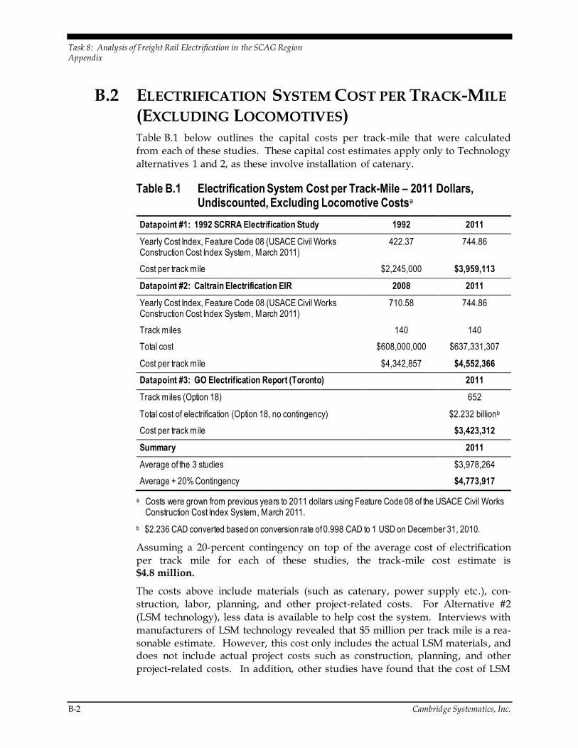
Task 8: Analysis of Freight Rail Electrification in the SCAG Region Appendix
B-2 Cambridge Systematics, Inc.
B.2 ELECTRIFICATION SYSTEM COST PER TRACK-MILE
(EXCLUDING LOCOMOTIVES) Table B.1 below outlines the capital costs per track-mile that were calculated
from each of these studies. These capital cost estimates apply only to Technology
alternatives 1 and 2, as these involve installation of catenary.
Table B.1 Electrification System Cost per Track-Mile – 2011 Dollars, Undiscounted, Excluding Locomotive Costsa
Datapoint #1: 1992 SCRRA Electrification Study 1992 2011
Yearly Cost Index, Feature Code 08 (USACE Civil Works Construction Cost Index System, March 2011)
422.37 744.86
Cost per track mile $2,245,000 $3,959,113
Datapoint #2: Caltrain Electrification EIR 2008 2011
Yearly Cost Index, Feature Code 08 (USACE Civil Works Construction Cost Index System, March 2011)
710.58 744.86
Track miles 140 140
Total cost $608,000,000 $637,331,307
Cost per track mile $4,342,857 $4,552,366
Datapoint #3: GO Electrification Report (Toronto) 2011
Track miles (Option 18) 652
Total cost of electrification (Option 18, no contingency) $2.232 billionb
Cost per track mile $3,423,312
Summary 2011
Average of the 3 studies $3,978,264
Average + 20% Contingency $4,773,917
a Costs were grown from previous years to 2011 dollars using Feature Code 08 of the USACE Civil Works Construction Cost Index System, March 2011.
b $2.236 CAD converted based on conversion rate of 0.998 CAD to 1 USD on December 31, 2010.
Assuming a 20-percent contingency on top of the average cost of electrification
per track mile for each of these studies, the track-mile cost estimate is $4.8 million.
The costs above include materials (such as catenary, power supply etc.), con-
struction, labor, planning, and other project-related costs. For Alternative #2
(LSM technology), less data is available to help cost the system. Interviews with
manufacturers of LSM technology revealed that $5 million per track mile is a rea-
sonable estimate. However, this cost only includes the actual LSM materials, and does not include actual project costs such as construction, planning, and other
project-related costs. In addition, other studies have found that the cost of LSM

Task 8: Analysis of Freight Rail Electrification in the SCAG Region Appendix
Cambridge Systematics, Inc. B-3
can range between $10 million to $20 million for materials only.26 In summary,
per track-mile project costs are unclear for LSM technology. LSM materials cost
estimates alone range from $5 million to $20 million, with unknown additional project costs. For comparative purposes, the full project cost of a track-mile of
LSM would end up being more than the cost of installation of the other two
technologies, even if the lowest cost were estimated.
B.3 TOTAL ELECTRIFICATION SYSTEM COST
(EXCLUDING LOCOMOTIVES) The next step is to apply these estimates to the total track-miles per option. Mul-
tiplying the track-miles per option by the track-mile cost gives us the estimated
total cost (in 2011 dollars) of electrifying each option. Table B.2 below highlights the track-miles per option.
Table B.2 Electrification System Track-Miles
Option Track-Miles
Option I Total Track Miles (Full AC) 60
Option I Total Track Miles (start 3 miles north of Ports) 51
Option II Total Track Miles 422
Option III Total Track Miles 863
Cost of Locomotives Required: Determining the Cost of New Locomotives Required for Each Option and Technology Alternative
The cost of locomotives is the other major capital cost consideration for rail elec-
trification. General assumptions for locomotive costs are discussed here by the
type of technology.
1. Straight-electric (electrified catenary). The locomotive counts presented in
Appendix A will be utilized to estimate the cost of straight-electric locomo-tives. It is assumed that nearly all of the current diesel line-haul freight
locomotives will be moved out of the region and will need to be replaced by
straight-electric locomotives. No changes will be made to the switcher or
Class II/III fleets.
2. Dual-mode locomotives (electrified catenary). Similar to the straight-electric option above, a requirement would be to replace existing line-haul
locomotives that operate in the SCAG region with dual-mode locomotives
26“Alternative Container Transportation Technology Evaluation and Comparison”.

Task 8: Analysis of Freight Rail Electrification in the SCAG Region Appendix
B-4 Cambridge Systematics, Inc.
prior to starting electric freight rail service in the SCAG region. For the pur-
poses of this analysis, it is assumed that the same numbers of locomotives
that are required in terms of straight-electric locomotives are required for dual-mode locomotives. It is important to note that if a strategy utilizing
dual-mode locomotives was selected, it could make sense to replace the
majority of the line-haul fleet with dual-modes, so that locomotives can be
used interchangeably on a corridor or on the entire system. However, for the purposes of costing locomotives, it will only be assumed that enough
locomotives to move trains effectively for each electrification option are
required.
3. LSM system. For this option, it is assumed that zero electric or Tier IV line-
haul locomotives would be required within the electrified areas (unless the railroads were to determine that moving idling or off diesel locomotives
would make sense from an operations perspective). General Atomics
revealed that “helper cars” or “power cars” that are equipped with magnets
would be required to propel the train along the tracks. Further information
is needed to estimate costs of LSM helper cars.
Given these assumptions, Table B.3 below highlights the estimated cost per
locomotive or helper car for each technology. These are per unit costs for each
type of locomotive. As technologies mature, such as dual-mode and straight-
electric locomotive technologies for the North American freight market, it is likely that the price of these units will decrease.
Table B.3 Cost per Locomotive Unit
Technology Cost per Unit 2011 Dollars
Tier IV Locomotive (base case) $3.5 milliona
Straight-Electric Locomotive $5.0 millionb
Dual-Mode Locomotive $8.0 millionc
LSM Helper Car Unknownd
a California Air Resources Board.
b The cost of full electric locomotives was derived through research and interviews with industry experts. The $5 million cost for full electric locomotives was derived from a locomotive manufacturer interview in June 2011. It should be
noted that this is an estimate, and that costs may be significantly higher or lower, dependent on several items, including: a) potential discount for volume purchase of locomotives; b) potential discount if buying from Chinese or other countries where the cost of manufacturing is low; c) potential increase in cost if the effort to adjust freight locomotives to meet U.S. freight rail standards is higher than expected.
c The cost of a large order of dual-mode locomotives was estimated using reported price for the options purchase of
Bombardier ALP-45DP locomotives by NJ Transit in 2010, http://www.railwaygazette.com/nc/news/single-view/view/nj-transit-approves-fy2011-spending.html. This cost was grown to 2011 dollars. It should be noted that this is just a snapshot of what a dual-mode locomotive might cost. Economies of scale may decrease the cost of these units in the future. On the other hand, technological difficulties in designing and constructing a dual -mode freight locomotive for
the U.S. long-haul freight market might prove to be costly, which could result in higher prices.
d There is a high degree of uncertainty regarding the cost of an LSM helper car. Interviews with LSM manufacturers suggested that the cost of such a car could cost significantly less than a locomotive.

Task 8: Analysis of Freight Rail Electrification in the SCAG Region Appendix
Cambridge Systematics, Inc. B-5
Table B.4 Total Locomotive Cost Through 2035 (Undiscounted)
Estimated Cost
Straight-Electric Locomotive
Cost per locomotive $5,000,000
Option I Estimate Total Electrification Cost ($2011) $618,233,012
Option II Estimate Total Electrification Cost ($2011) $4,742,052,643
Option III Estimate Total Electrification Cost ($2011) $9,565,589,315
Dual-Mode Locomotive
Cost per dual-mode locomotive $8,000,000
Option I Estimate Total Electrification Cost ($2011) $989,172,820
Option II Estimate Total Electrification Cost ($2011) $7,587,284,229
Option III Estimate Total Electrification Cost ($2011) $15,304,942,905
Given this data, estimates of total cost (through 2035) are determined by adding the general electrification costs and the locomotive costs (through 2035).


Task 8: Analysis of Freight Rail Electrification in the SCAG Region Appendix
Cambridge Systematics, Inc. C-1
C. Energy Needs to Power Electrification System
There are a number of assumptions that need to be taken to estimate energy needs for an electrified rail system in the future, given current data limitations.
This information is needed to help calculate emissions from electrification as well
to help understand energy cost impacts. Note that there can be substantial dif-
ferences based on the current efficiency of diesel locomotives, electric locomo-tives, transmission losses and other factors. This analysis provides a reasonable
estimate of energy required to power an electrified system, but further analysis
and cooperation between SCAG, the railroads, locomotive manufacturers and
utilities in the region could yield a more precise estimate.
Energy costs for electrified rail and for standard diesel were calculated using the following data components:
Railroad diesel price projections were drawn from a February 2011 California
Energy Commission (CEC) staff report titled “Transportation Fuel Price Cases
and Demand Scenarios: Inputs and Methods for the 2011 Integrated Energy Policy Report.”27 Both “high” and “low” estimates are available through 2030. Please see Table C.1 below for railroad diesel fuel price projections.
27 CEC web site: http://www.energy.ca.gov/2011publications/CEC-600-2011-001/CEC-600-2011-001.PDF

Task 8: Analysis of Freight Rail Electrification in the SCAG Region Appendix
C-2 Cambridge Systematics, Inc.
Table C.1 Projected Railroad Diesel Prices (2010 Cents per Gallon)a
Year High Price Low Price Year High Price Low Price
2011 307 262 2031 422 257
2012 332 266 2032 428 256
2013 346 270 2033 435 256
2014 360 274 2034 442 256
2015 370 278 2035 449 256
2016 374 276 2036 456 255
2017 376 274 2037 464 255
2018 379 273 2038 471 255
2019 379 271 2039 479 255
2020 380 269 2040 486 254
2021 381 266 2041 494 254
2022 382 262 2042 502 254
2023 383 258 2043 510 254
2024 386 255 2044 518 253
2025 389 251 2045 527 253
2026 392 252 2046 535 253
2027 398 253 2047 544 253
2028 404 255 2048 552 252
2029 408 256 2049 561 252
2030 415 257 2050 570 252
Source: California Energy Commission
a Prices assume sales tax of 8.25 percent. To estimate costs from 2036-2050, the compound annual
growth rate for both the “High” and “Low” scenarios from 2011 to 2035 were utilized.
The price of electricity was also provided by the CEC. For the purposes of a large demand generator such as a rail electrification project, “industrial” electricity rates were used as a proxy for what the railroads would pay per
kWh of electricity. Table C.2 below shows the price per kWh for low,
medium and high demand scenarios. The projections only go through 2022,
so the compound average growth rate from 2011 to 2022 was applied to the years 2023 through 2030.

Task 8: Analysis of Freight Rail Electrification in the SCAG Region Appendix
Cambridge Systematics, Inc. C-3
Table C.2 Projected Price of Electricity for Southern California Edison (2010 Cents per kWh)
Year
Low
Demand Scenario
Mid
Demand Scenario
High
Demand Scenario Year
Low
Demand Scenario
Mid
Demand Scenario
High
Demand Scenario
2010 9.05 9.05 9.05 2031 12.92 11.22 9.98
2011 9.05 9.05 9.05 2032 13.14 11.33 10.03
2012 9.27 8.84 8.67 2033 13.36 11.45 10.08
2013 9.49 8.98 8.74 2034 13.59 11.57 10.12
2014 9.72 9.11 8.82 2035 13.82 11.69 10.17
2015 9.92 9.22 8.89 2036 14.06 11.81 10.22
2016 10.07 9.33 8.96 2037 14.30 11.93 10.27
2017 10.23 9.44 9.04 2038 14.55 12.05 10.32
2018 10.39 9.57 9.11 2039 14.79 12.18 10.36
2019 10.56 9.69 9.18 2040 15.05 12.30 10.41
2020 10.75 9.85 9.26 2041 15.31 12.43 10.46
2021 10.91 10.04 9.42 2042 15.57 12.56 10.51
2022 11.09 10.23 9.57 2043 15.83 12.69 10.56
2023 11.28 10.34 9.61 2044 16.10 12.82 10.61
2024 11.47 10.44 9.66 2045 16.38 12.95 10.66
2025 11.67 10.55 9.71 2046 16.66 13.08 10.71
2026 11.87 10.66 9.75 2047 16.94 13.22 10.76
2027 12.07 10.77 9.80 2048 17.23 13.35 10.81
2028 12.28 10.88 9.84 2049 17.53 13.49 10.86
2029 12.49 10.99 9.89 2050 17.83 13.63 10.91
2030 12.70 11.10 9.94
Source: Price Scenarios from California Energy Commission (CEC) staff analysis. CEC staff estimates were developed through 2022. For 2023 through 2050, electricity prices were grown by applying the compound annual growth rate of prices from 2010 to 2023. Please note that this is not an
official CEC forecast of electricity prices. Numbers through 2022 were generated by CEC staff utilizing the E3 Calculator, http://www.ethree.com/public_projects/cpuc4.html.
The gallons of diesel consumed annually in the South Coast Air Basin (SCAB) are calculated by utilizing locomotive diesel consumption factors
provided by the California Air Resources Board (ARB) and are grown using
the expected locomotive-miles growth rate, based on Dr. Leachman28 train
counts and CS analysis to get total locomotive miles. Annually, the ARB
estimates that 50,000 gallons of fuel are consumed by each of the 660 freight locomotives (in year 2010) that operate in the SCAB on any given day. While
28 2011 Regional Rail Simulation Update, SCAG Comprehensive Regional Goods Movement Plan and
Implementation Strategy. Prepared for SCAG by Dr. Robert Leachman, Leachman and Associates, LLC.

Task 8: Analysis of Freight Rail Electrification in the SCAG Region Appendix
C-4 Cambridge Systematics, Inc.
gallons of diesel is the necessary value to help estimate price, it is necessary
to convert gallons of diesel to kWh to energy units to understand the amount
of energy required to power trains in the region. This helps with the calcula-tion of kWh required for an electrified rail system, as discussed below.
The kWh of electricity that would be consumed with an electrified system is
calculated by taking several steps. First, it is assumed that the energy
required to power all diesel trains currently moving in the SCAB (and for each electrification option) is equivalent to the energy required to power the
same number of trains in the future. However, there will be differences in
amount of energy consumed primarily because the efficiency of an electrified
rail system is different than the efficiency of the process of converting gallons of diesel into traction on current locomotives. Two further assumptions were
made based on available data and as a result of input from interviews:
– Efficiency of a diesel engine in an average duty cycle: While this is
highly variable by locomotive type and by the terrain on which the loco-
motive is operating, this is estimated based on a standard value of brake-specific fuel consumption (BSFC) data provided by ARB. As a result of
this input, it is estimated that the efficiency of a diesel engine is 38.2 percent.
– Efficiency of an electric locomotive and line loss between powerplant and the locomotive: From an interview with Siemens (interview with
staff on July 15, 2011), it was estimated that the efficiency with which
straight-electric engines process electricity into traction is 86 percent. In
addition, line loss (loss of energy during the transmission from the power
generation facility to the locomotive) was estimated at 7 percent. There-fore, the efficiency of an electric system in converting energy is estimated
at 79 percent. Further, it is assumed that one-half of this loss occurs
between substation and locomotive. This is only the efficiency of con-
verting energy to traction AFTER energy production at the powerplant. Since the purpose of this portion of the analysis is focused on energy
costs, there is no need to account for inefficiency of the production of
energy at powerplants. The railroads do not pay for energy lost during
production directly – they only pay for energy lost after the energy was
produced and delivered to the substation.
Utilizing these factors allows for an estimate of the amount of energy required if
an electrified system were to be developed in the SCAG region. This is adjusted
by electrification option and by year.
As a result of the data above, the first number that can be calculated is the “break-even” price point ($/kWh) at which an electrified rail system would
become more affordable than running the system with diesel locomotives. This
analysis is shown in Table C.3 for Option III below, for both high and low diesel
price estimates. See the last and third-to-last columns. For instance, this indi-
cates that in 2023, given a diesel price of $3.83 per gallon, the average price per

Task 8: Analysis of Freight Rail Electrification in the SCAG Region Appendix
Cambridge Systematics, Inc. C-5
kWh of electricity would need to be $0.20 or less for the railroads to break even
in terms of energy expenses in the SCAG region.


Task 8: Analysis of Freight Rail Electrification in the SCAG Region Appendix
Cambridge Systematics, Inc. C-7
Table C.3 Option III Straight-Electric/Dual-Mode Technology, Line-Haul Locomotive Break-Even Energy Price Analysis
Year Diesel Gallons
Required
Electricity Required
(kWh) to Power Electric System
Diesel Prices
(2010 Dollars, High Scenario)
Diesel Prices
(2010 Dollars, Low Scenario)
Break-Even per kWh
Electricity Cost (2010 Dollars/kWh,
High Scenario)
Break-Even per kWh
Electricity Cost (2010 Dollars/kWh,
Low Scenario)
2011 49,969,642 939,302,948 3.07 2.62 0.16 0.14
2012 51,808,837 973,875,155 3.32 2.66 0.18 0.14
2013 53,715,725 1,009,719,835 3.46 2.70 0.18 0.14
2014 55,692,799 1,046,883,822 3.60 2.74 0.19 0.15
2015 57,742,641 1,085,415,676 3.70 2.78 0.20 0.15
2016 59,867,931 1,125,365,742 3.74 2.76 0.20 0.15
2017 62,071,444 1,166,786,220 3.76 2.74 0.20 0.15
2018 64,356,060 1,209,731,230 3.79 2.73 0.20 0.15
2019 66,724,765 1,254,256,884 3.79 2.71 0.20 0.14
2020 69,180,652 1,300,421,360 3.80 2.69 0.20 0.14
2021 71,726,931 1,348,284,976 3.81 2.66 0.20 0.14
2022 74,366,930 1,397,910,272 3.82 2.62 0.20 0.14
2023 77,104,097 1,449,362,089 3.83 2.58 0.20 0.14
2024 79,942,008 1,502,707,653 3.86 2.55 0.21 0.14
2025 82,884,373 1,558,016,666 3.89 2.51 0.21 0.13
2026 85,935,035 1,615,361,397 3.92 2.52 0.21 0.13
2027 89,097,980 1,674,816,771 3.98 2.53 0.21 0.13
2028 92,377,341 1,736,460,473 4.04 2.55 0.21 0.14
2029 95,777,404 1,800,373,049 4.08 2.56 0.22 0.14
2030 99,302,609 1,866,638,005 4.15 2.57 0.22 0.14
2031 102,957,565 1,935,341,926 4.22 2.57 0.22 0.14
2032 106,747,045 2,006,574,579 4.28 2.56 0.23 0.14
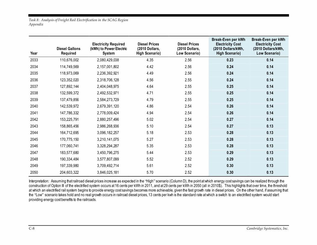
Task 8: Analysis of Freight Rail Electrification in the SCAG Region Appendix
C-8 Cambridge Systematics, Inc.
Year Diesel Gallons
Required
Electricity Required (kWh) to Power Electric
System
Diesel Prices (2010 Dollars,
High Scenario)
Diesel Prices (2010 Dollars, Low Scenario)
Break-Even per kWh Electricity Cost
(2010 Dollars/kWh, High Scenario)
Break-Even per kWh Electricity Cost
(2010 Dollars/kWh, Low Scenario)
2033 110,676,002 2,080,429,038 4.35 2.56 0.23 0.14
2034 114,749,569 2,157,001,802 4.42 2.56 0.24 0.14
2035 118,973,069 2,236,392,921 4.49 2.56 0.24 0.14
2036 123,352,020 2,318,706,128 4.56 2.55 0.24 0.14
2037 127,892,144 2,404,048,975 4.64 2.55 0.25 0.14
2038 132,599,372 2,492,532,971 4.71 2.55 0.25 0.14
2039 137,479,856 2,584,273,729 4.79 2.55 0.25 0.14
2040 142,539,972 2,679,391,120 4.86 2.54 0.26 0.14
2041 147,786,332 2,778,009,424 4.94 2.54 0.26 0.14
2042 153,225,791 2,880,257,496 5.02 2.54 0.27 0.14
2043 158,865,456 2,986,268,936 5.10 2.54 0.27 0.13
2044 164,712,695 3,096,182,257 5.18 2.53 0.28 0.13
2045 170,775,150 3,210,141,075 5.27 2.53 0.28 0.13
2046 177,060,741 3,328,294,287 5.35 2.53 0.28 0.13
2047 183,577,680 3,450,796,275 5.44 2.53 0.29 0.13
2048 190,334,484 3,577,807,099 5.52 2.52 0.29 0.13
2049 197,339,980 3,709,492,714 5.61 2.52 0.30 0.13
2050 204,603,322 3,846,025,181 5.70 2.52 0.30 0.13
Interpretation: Assuming that railroad diesel prices increase as expected in the “High” scenario (Column D), the point at which energy cost savings can be realized through the construction of Option III of the electrified system occurs at 16 cents per kWh in 2011, and at 29 cents per kWh in 2050 (all in 2010$). This highlights that over time, the threshold at which an electrified rail system begins to provide energy cost savings becomes more achievable, given the fast growth rate in diesel prices. On the other hand, if assuming that the “Low” scenario takes hold and no real growth occurs in railroad diesel prices, 13 cents per kwh is the standard rate at which a switch to an electrified system would start
providing energy cost benefits to the railroads.

Task 8: Analysis of Freight Rail Electrification in the SCAG Region Appendix
Cambridge Systematics, Inc. D-1
D. Calculation of Emissions Impacts
Calculating emissions data requires two key initial inputs:
1. Energy demand calculations (see Appendix C).
2. Calculation of emissions factors per GWh of electricity for CO2, NOx, and
PM2.5. Emissions factors were derived from several sources, mentioned in
the text. Table D.1 below highlights the emissions factors that were used in the analysis.
Table D.1 Key Factors Utilized to Calculate Emissions from Electrification
Total GHG Emissions (MMTCO2e/yr) 74.8
Total Electricity Generation (GWh/yr) 341,000
Total GHG Emissions from NG Baseload/Peaker (MMTCO2e/yr) 18.9
Total Electricity Generation (GWh/yr) 45,690
CO2 emissions (MMTCO2e) per GWh of electricity 0.0002193548
CO2 emissions (MMTCO2e) per GWh of electricity from natural gas 0.0004136573
NOx emissions from natural gas baseload generation per GWh (lbs/GWh)
250
PM2.5 emissions from natural gas baseload generation per GWh
(lbs/GWh) 50
These factors were then multiplied by the energy required for each phase of
electrification (normalized by locomotive miles) to generate annual emissions values for each electrification option, for each type of emission. Emission values
were only generated for 2023 (for Option I) and 2035 (for all Options). Various
types of emissions were also calculated for the analysis, as shown in the three
tables below. These emissions were then compared against baseline emissions to
understand emissions reduction as a result of electrification. This is discussed further in Section 4.0.

Task 8: Analysis of Freight Rail Electrification in the SCAG Region Appendix
D-2 Cambridge Systematics, Inc.
Table D.2 CO2 Daily Emissions per Electrification Option – Various Scenarios
2023 Option I – CO2 emissions per day (short tons CO2e/day) 86.73
2023 Option I – CO2 emissions per day (short tons NOx /day) emitted in SCAB, assuming 30 percent of electricity produced in SCAB by natural gas generators 26.02
2035 Option I – CO2 emissions per day (short tons CO2e/day) 134.49
2035 Option I – CO2 emissions per day (short tons NOx /day) emitted in SCAB, assuming 30 percent of electricity produced in SCAB by natural gas generators 40.35
2035 Option II – CO2 emissions per day (short tons CO2e/day) 710.72
2035 Option II – CO2 emissions per day (short tons NOx /day) emitted in SCAB, assuming 30 percent of electricity produced in SCAB by natural gas generators 213.22
2035 Option III – CO2 emissions per day (short tons CO2e/day) – produced from trains moving in SCAB 1,070.21
2035 Option III – CO2 emissions per day (short tons CO2e/day) – produced from trains
moving outside the SCAB 507.64
2035 Option III – CO2 emissions per day (short tons CO2e/day) – produced from trains moving in/outside the SCAB 1,577.85
2035 Option III – CO2 emissions per day (short tons NOx /day) emitted in SCAB, assuming 30 percent of electricity produced in SCAB by natural gas generators 473.35
Table D.3 PM2.5 Daily Emissions per Electrification Option – Various Scenarios
2023 Option I – PM2.5 emissions per day (short tons PM 2.5/day) 0.009
2023 Option I – PM2.5 emissions per day (short tons NOx /day) emitted in SCAB, assuming 30 percent of electricity produced in SCAB by natural gas generators 0.003
2035 Option I – PM2.5 emissions per day (short tons PM 2.5/day) 0.014
2035 Option I – PM2.5 emissions per day (short tons NOx /day) emitted in SCAB, assuming 30 percent of electricity produced in SCAB by natural gas generators 0.004
2035 Option II – PM2.5 emissions per day (short tons PM 2.5/day) 0.07
2035 Option II – PM2.5 emissions per day (short tons NOx /day) emitted in SCAB, assuming
30 percent of electricity produced in SCAB by natural gas generators 0.02
Option III – PM2.5 emissions per day (short tons PM 2.5/day) produced from trains moving in
SCAB 0.11
Option III – PM2.5 emissions per day (short tons PM 2.5/day) produced from trains moving in/outside of SCAB 0.16
Option III – PM2.5 emissions per day (short tons NOx /day) emitted in SCAB, assuming 30 percent of electricity produced in SCAB by natural gas generators 0.05

Task 8: Analysis of Freight Rail Electrification in the SCAG Region Appendix
Cambridge Systematics, Inc. D-3
Table D.4 NOx Daily Emissions per Electrification Option – Various Scenarios
2023 Option I – NOx emissions per day (short tons NOx /day) 0.045
2023 Option I – NOx emissions per day (short tons NOx /day) emitted in SCAB, assuming 30 percent of electricity produced in SCAB by natural gas generators 0.01
2035 Option I – NOx emissions per day (short tons NOx /day) 0.070
2035 Option I – NOx emissions per day (short tons NOx /day) emitted in SCAB, assuming 30 percent of electricity produced in SCAB by natural gas generators 0.021
2035 Option II – NOx emissions per day (short tons NOx /day) 0.37
2035 Option II – NOx emissions per day (short tons NOx /day) emitted in SCAB, assuming 30 percent of electricity produced in SCAB by natural gas generators 0.11
Option III – NOx emissions per day (short tons NOx /day) produced from trains moving in SCAB 0.55
Option III – NOx emissions per day (short tons NOx /day) produced from trains moving
in/outside of SCAB 0.82
Option III – NOx emissions per day (short tons NOx /day) emitted in SCAB, assuming 30 percent of electricity produced in SCAB by natural gas generators 0.24