task 38 solar air-conditioning and...
TRANSCRIPT

IEA SHC Task 38 Solar Air Conditioning and Refrigeration Subtask C2-A, November 9, 2009
page 1
Task 38Solar Air -Conditioningand Refr igeration
Description of simulation tools used in solar cooli ng
New developments in simulation tools and models and their validation
Solid desiccant cooling
Absorption chiller
A technical report of subtask C Deliverable C2-A Date: Novembre 9, 2009
By
Paul Bourdoukan 1
Contributions by Edo Wiemken 2, Paul Kohlenbach 3, Etienne Wurtz 4, Harald Moser 5, Alexander Morgenstern 6, Antoine Dalibard 7, Felix Ziegler 8, Constanze Bongs 9 1 LOCIE FRE CNRS 3220, Institut National de l'Energie Solaire (INES), Tel: +33 (0)4 79444545 Fax: +33 (0)4 79 253690 Email: [email protected] 2 Fraunhofer Institute for Solar Energy Systems ISE, Freiburg, Germany Tel: +49 761 4588 5412 Fax: +49 761 4588 9000 Email: [email protected] 3 Solem Consulting
Postfach 2127, 71370 Weinstadt, Germany Tel:+49 (0)174/ 41 30 92 1 Fax:+49 (0)7151/ 60 48 62 5 Email: [email protected] 4 LOCIE FRE CNRS 3220, Institut National de l'Energie Solaire (INES), Tel: + 33 (0) 4 79444554 Fax:+ 33 (0) 4 79253690 Email: [email protected]

IEA SHC Task 38 Solar Air Conditioning and Refrigeration Subtask C2-A, November 9, 2009
page 2
5 Graz University of Technology, Institute of Thermal Engineering, Austria Tel: +43 316 873 7304 Fax:+43 316 873 7305 Email: [email protected] 6 Fraunhofer Institute for Solar Energy Systems ISE, Freiburg, Germany Tel: +49 761 4588 5107 Fax:+49 761 4588 9000 Email: [email protected] 7 ZAFH.NET (Stuttgart University of Applied Sciences)
Tel: +49 (0)711/ 89 26-29 81 Fax: +49 (0)711/ 89 26-26 98 Email: [email protected] 8 Technische Universität Berlin, Institute for Energy Engineering Tel: 314-25624 Fax: 314-22253 Email: [email protected] 6 Fraunhofer Institute for Solar Energy Systems ISE, Freiburg, Germany Tel: +49 761 4588 5487 Fax:+49 761 4588 9000 Email: [email protected]

IEA SHC Task 38 Solar Air Conditioning and Refrigeration Subtask C2-A, November 9, 2009
page 3
Content
Introduction ........................................................................................................................... 5
Chapter I: Description of simulation software, applicable for solar cooling ............................. 7
SPARK............................................................................................................................... 8
EnergyPlus........................................................................................................................10
EES...................................................................................................................................12
TRNSYS ...........................................................................................................................14
EASYCOOL ......................................................................................................................15
INSEL ...............................................................................................................................17
Chapter II: New developments in simulations tools and models A solar desiccant cooling
installation model in SPARK, A transient detailed model of the desiccant wheel. ................21
1. Modelling of the solar desiccant cooling installation.......................................................23
2. Experimental validation .................................................................................................34
3. Transient model of the desiccant wheel and experimental validation.............................46
Chapter III: New developments in simulation tools and models: A dynamic simulation model
for transient absorption chiller performance..........................................................................59
1. A dynamic simulation model for transient absorption chiller performance. Part 1: the
model ................................................................................................................................60
2. A dynamic simulation model for transient absorption chiller performance: Numerical
results and experimental verification .................................................................................79
Conclusion ...........................................................................................................................95

IEA SHC Task 38 Solar Air Conditioning and Refrigeration Subtask C2-A, November 9, 2009
page 4

IEA SHC Task 38 Solar Air Conditioning and Refrigeration Subtask C2-A, November 9, 2009
page 5
Introduction
Numerical simulation offers the possibility to study virtually physical systems and to test
rapidly the proposed solutions. Simulation is then the most adapted method to understand
the behaviour of a system in order to optimize it. The enhancement and the development of a
technology are essentially based on the capacity to simulate accurately its behaviour in order
to optimize it. This reality applies to solar cooling technologies.
In this report simulation tools used in the solar cooling domains are described. Then the
recent development in the components and system models and validation are presented.
In part 1 of the report the simulation tools applicable in the domain of solar cooling are
presented and the main advantages of each tool are highlighted.
Part 2 concerns the recent developments in modelling solid desiccant cooling technologies
and the vacuum tube solar collectors with an experimental validation of an implementation in
the SPARK simulation environment. Part 3 presents a recent transient model of the Li/Br
absorption chiller with an experimental validation.
Each part has its reference section and conclusion.
This report and the authors don’t pretend to include all the simulation tools used in solar
cooling or all the recent models related to solid desiccant cooling and absorption chiller. The
simulation tools described in this report are those identified and used by the participants of
the IEA Task 38.

IEA SHC Task 38 Solar Air Conditioning and Refrigeration Subtask C2-A, November 9, 2009
page 6
IEA SHC Task 38 Solar Air Conditioning and Refrigeration Subtask C2-A, November 9, 2009
page 7
Chapter I: Description of simulation software, appl icable for solar cooling
In this chapter a brief description of some simulation tools applicable in solar cooling is given.
These tools are the most commonly used by IEA Task 38 participants. The range goes from
predefined simple configuration software to low level equation solver. Some of the tools are
developed by research groups and are dedicated for internal use and other are commercially
available software. The simulation tools highlighted here are SPARK, EnergyPlus, EES,
EasyCool, TRNSYS and INSEL.

IEA SHC Task 38 Solar Air Conditioning and Refrigeration Subtask C2-A, November 9, 2009
page 8
SPARK Paul Bourdoukan and Etienne Wurtz, LOCIE FRE CNRS 3220, Institut National de l’Energie Solaire SPARK is a general simulation environment that supports the definition of simulation models and solution of these models via a robust and efficient differential/algebraic equation solver. In SPARK, the modeller describes the set of equations defining a model as equation-based objects. At the lowest level, an atomic object characterizes one equation and its variables. Then, macroscopic objects can be created as an assembly of various atomic or macroscopic objects. The entire model is built by connecting the different necessary objects. If one class of objects needs to be reused, it can be instantiated as many times as required, without any additional effort. At this stage, it is necessary to observe that the model is input/output free. The particular problem to be solved is then described by imposing the adequate input data (boundary and initial conditions) and by specifying the variables to be solved. So in this environment it is not necessary to order the equations or to express them as assignments statements (algorithms) in opposition to conventional modular environments such as Matlab/Simulink or TRNSYS. SPARK uses a mathematical graph of the model to decompose it as strong components to be solved independently. Within each component, SPARK finds the appropriate function call sequence to get the solution. If no direct sequence is possible, as evidence by a cyclic problem graph, a small “cut set” is determined so as to minimize the number of variables involved in the Newton-like iterative numerical solution process. As a result, this decreases the size of the Jacobian matrix involved in the Newton iteration within the component. Consequently, the way SPARK handles the solution of coupled nonlinear equations makes it a fast solver for building energy simulation problems. Since the “cut sets” of variables have been identified, the problem specification file is converted into a C++ program which is then compiled, linked and executed to solve the problem for given boundary and initial conditions.
SPARK is free and has a detailed reference manual. Using SPARK requires a 3 to 5 months learning period to be able to create models. A support service is available and provided by the simulation research group (SRG) of the Lawrence Berkeley National Laboratory (LBNL)
SPARK has it’s own HVAC library based on some simple models. However various doctoral researches in the domain of building physics and HVAC systems were accomplished using SPARK as a simulation environment [1], [2], [3], [4], [5] and [6]. This allowed the creation of models library for the building envelope [1], [2] and [3], and a library for the systems [4], [5] and [6]. Recently works [4], [5] were developed on solar desiccant cooling beside an on going PhD thesis on absorption chillers powered by solar collectors. However all these models are dedicated for internal use but can be distributed by their developers.
Important links http://gundog.lbl.gov/VS/spark.html (download) http://simulationresearch.lbl.gov/dirpubs/spkall.html (reference manual)
References
[1]. Musy, M. « Génération automatique de modèles zonaux pour l’étude du
comportement thermo-aéraulique des bâtiments ». PhD thesis, Université de La
Rochelle, France. (1999).

IEA SHC Task 38 Solar Air Conditioning and Refrigeration Subtask C2-A, November 9, 2009
page 9
[2]. Mora, L. « Prédiction des performances thermo-aérauliques des bâtiments par
association de modèles de différents niveaux de finesse au sein d’un
environnement ». PhD thesis, Université La Rochelle, France (2003).
[3]. Cordeiro Mendonça, K. « Modélisation thermo-hydro-aéraulique des locaux
climatisés selon l’approche zonale (prise en compte des phénomènes de sorption
d’humidité) ». PhD thesis, Université La Rochelle, France (2004).
[4]. Maalouf, C. « Étude du potentiel de rafraîchissement d’un système évaporatif
àdésorption avec régénération solaire ». PhD thesis, Université de La Rochelle,
France (2006)
[5]. Bourdoukan. P. « Etude numérique et expérimentale destinée à l’exploitation des
techniques de rafraîchissement par dessiccation avec régénération par énergie
solaire ». Ph.D thesis, Université La Rochelle, (2008) (Available in English)
[6]. Tittelin, P. « Environnements de simulation adaptés à l’étude du comportement énergétique des bâtiments basse consommation ». PhD thesis, Université de Savoie, France (2008)

IEA SHC Task 38 Solar Air Conditioning and Refrigeration Subtask C2-A, November 9, 2009
page 10
EnergyPlus Paul Bourdoukan and Etienne Wurtz LOCIE FRE CNRS 3220, Institut National de l’Energie Solaire EnergyPlus has its roots in both the BLAST and DOE–2 programs. BLAST (Building Loads Analysis and System Thermodynamics) and DOE–2 were both developed and released in the late 1970s and early 1980s as energy and load simulation tools. Their intended audience is a design engineer or architect that wishes to size appropriate HVAC equipment, develop retrofit studies for life cycling cost analyses, optimize energy performance, etc. Born out of concerns driven by the energy crisis of the early 1970s and recognition that building energy consumption is a major component of the American energy usage statistics, the two programs attempted to solve the same problem from two slightly different perspectives. Both programs had their merits and shortcomings, their supporters and detractors, and solid user bases both nationally and internationally. Like its parent programs, EnergyPlus is an energy analysis and thermal load simulation program. Based on a user’s description of a building from the perspective of the building’s physical make-up, associated mechanical systems, etc., EnergyPlus will calculate the heating and cooling loads necessary to maintain thermal control setpoints, conditions throughout an secondary HVAC system and coil loads, and the energy consumption of primary plant equipment as well as many other simulation details that are necessary to verify that the simulation is performing as the actual building would. Many of the simulation characteristics have been inherited from the legacy programs of BLAST and DOE–2. Below is list of some of the features of the first release of EnergyPlus. While this list is not exhaustive, it is intended to give the reader and idea of the rigor and applicability of EnergyPlus to various simulation situations.
• Integrated, simultaneous solution where the building response and the primary and secondary systems are tightly coupled (iteration performed when necessary)
• Sub-hourly, user-definable time steps for the interaction between the thermal zones and the environment; variable time steps for interactions between the thermal zones and the HVAC systems (automatically varied to ensure solution stability)
• ASCII text based weather, input, and output files that include hourly or sub-hourly environmental conditions, and standard and user definable reports, respectively
• Heat balance based solution technique for building thermal loads that allows for simultaneous calculation of radiant and convective effects at both in the interior and exterior surface during each time step
• Transient heat conduction through building elements such as walls, roofs, floors, etc.using conduction transfer functions
• Improved ground heat transfer modeling through links to three-dimensional finite difference ground models and simplified analytical techniques
• Combined heat and mass transfer model that accounts for moisture adsorption/desorption either as a layer-by-layer integration into the conduction transfer functions or as an effective moisture penetration depth model (EMPD)
• Thermal comfort models based on activity, inside dry bulb, humidity, etc. • Anisotropic sky model for improved calculation of diffuse solar on tilted surfaces • Advanced fenestration calculations including controllable window blinds,
electrochromic glazings, layer-by-layer heat balances that allow proper assignment of solar energy absorbed by window panes, and a performance library for numerous commercially available windows
• Daylighting controls including interior illuminance calculations, glare simulation and control, luminaire controls, and the effect of reduced artificial lighting on heating and cooling

IEA SHC Task 38 Solar Air Conditioning and Refrigeration Subtask C2-A, November 9, 2009
page 11
• Loop based configurable HVAC systems (conventional and radiant) that allow users to model typical systems and slightly modified systems without recompiling the program source code
• Atmospheric pollution calculations that predict CO2, SOx, NOx, CO, particulate matter, and hydrocarbon production for both on site and remote energy conversion
• Links to other popular simulation environments/comp onents such as WINDOW5, DElight and SPARK to allow more detailed analysis of building components More details on each of these features can be found in the various parts of the EnergyPlus documentation library.
No program is able to handle every simulation situation. However, it is the intent of EnergyPlus to handle as many building and HVAC design options either directly or indirectly through links to other programs in order to calculate thermal loads and/or energy consumption on for a design day or an extended period of time (up to, including, and beyond a year). While the first version of the program contains mainly features that are directly linked to the thermal aspects of buildings, future versions of the program will attempt to address other issues that are important to the built environment: water, electrical systems, etc.
References: http://www.energyplus.gov/pdfs/gettingstarted.pdf http://www.eere.energy.gov/buildings/energyplus/cfm/reg_form.cfm (Link for download)

IEA SHC Task 38 Solar Air Conditioning and Refrigeration Subtask C2-A, November 9, 2009
page 12
EES
Harald Moser, Graz TU
Graz University of Technology, Institute of Thermal Engineering, Austria
EES is an acronym for Engineering Equation Solver. The basic function provided by EES is the numerical solution of a set of algebraic equations. EES can also be used to solve differential and integral equations, do optimization, provide uncertainty analyses and linear and non-linear regression, convert units and check unit consistency and generate publication-quality plots.
There are two major differences between EES and other equation-solving programs:
1. EES allows equations to be entered in any order with unknown variables placed anywhere in the equations; EES automatically reorders the equations for efficient solution.
2. EES provides many built-in mathematical and thermophysical property functions useful for engineering calculations. For example, the steam tables are implemented such that any thermodynamic property can be obtained from a built-in function call in terms of any two other properties. Similar capability is provided for most refrigerants, ammonia, methane, carbon dioxide and other fluids. Air tables are built-in, as are psychrometric functions and JANAF data for many common gases. Transport properties are also provided for all substances.
The available built-in thermophysical property functions are listed below in alphabetical order. Additional fluid property data can be added by the user.
EES built-in thermophysical property functions
ACENTRICFACTOR CONDUCTIVITY CP
CV DENSITY DEWPOINT
DIPOLE ENTHALPY ENTHALPY_FUSION
ENTROPY FUGACITY HUMRAT (humidity ratio)
INTENERGY ISIDEALGAS MOLARMASS
PRANDTL PRESSURE P_CRIT
P_SAT QUALITY RELHUM
SOUNDSPEED SPECHEAT SURFACETENSION
TEMPERATURE T_CRIT T_SAT
T_TRIPLE VISCOSITY WETBULB
VOLUME V_CRIT VOLEXPCOEF
The built-in thermophysical property data for the fluids listed below are provided by EES.
IEA SHC Task 38 Solar Air Conditioning and Refrigeration Subtask C2-A, November 9, 2009
page 13
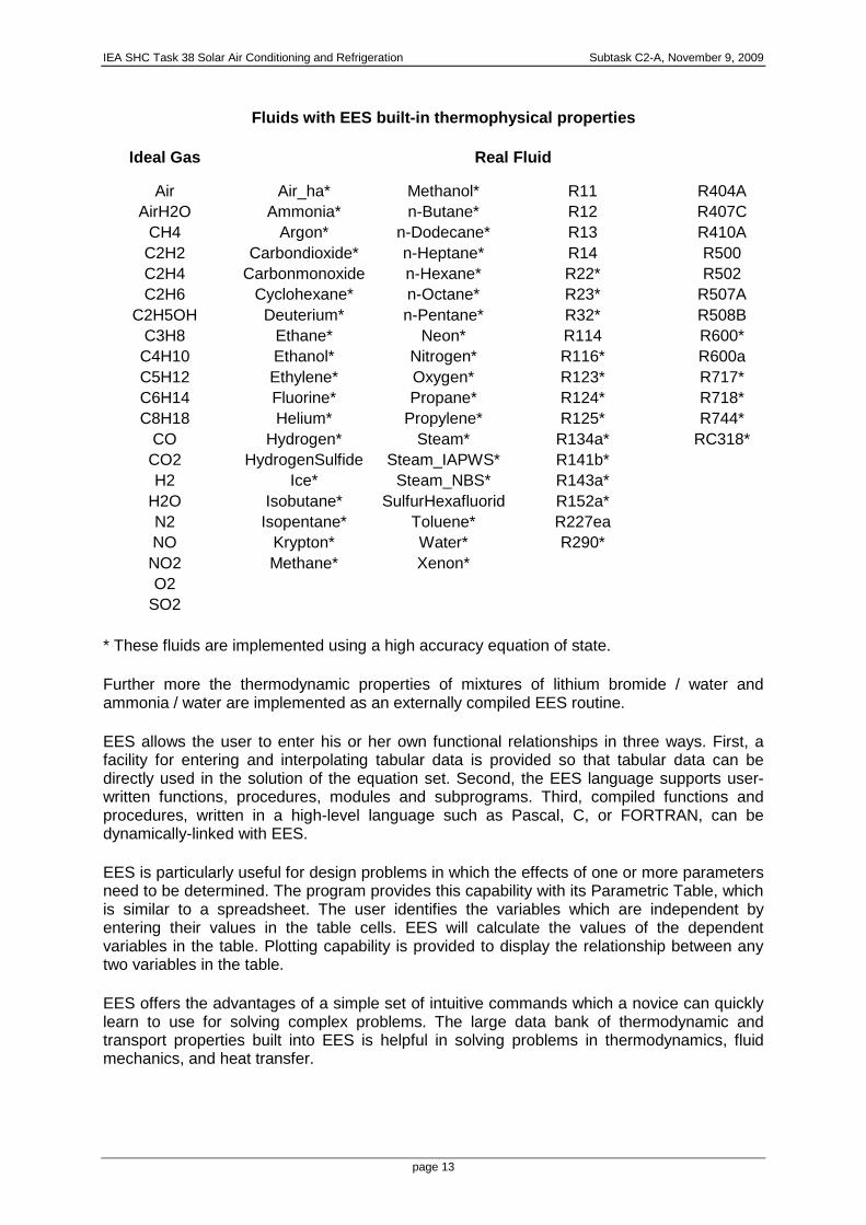
Fluids with EES built-in thermophysical properties
Ideal Gas Real Fluid
Air Air_ha* Methanol* R11 R404A AirH2O Ammonia* n-Butane* R12 R407C
CH4 Argon* n-Dodecane* R13 R410A C2H2 Carbondioxide* n-Heptane* R14 R500 C2H4 Carbonmonoxide n-Hexane* R22* R502 C2H6 Cyclohexane* n-Octane* R23* R507A
C2H5OH Deuterium* n-Pentane* R32* R508B C3H8 Ethane* Neon* R114 R600* C4H10 Ethanol* Nitrogen* R116* R600a C5H12 Ethylene* Oxygen* R123* R717* C6H14 Fluorine* Propane* R124* R718* C8H18 Helium* Propylene* R125* R744*
CO Hydrogen* Steam* R134a* RC318* CO2 HydrogenSulfide Steam_IAPWS* R141b* H2 Ice* Steam_NBS* R143a*
H2O Isobutane* SulfurHexafluorid R152a* N2 Isopentane* Toluene* R227ea NO Krypton* Water* R290* NO2 Methane* Xenon* O2
SO2
* These fluids are implemented using a high accuracy equation of state.
Further more the thermodynamic properties of mixtures of lithium bromide / water and ammonia / water are implemented as an externally compiled EES routine.
EES allows the user to enter his or her own functional relationships in three ways. First, a facility for entering and interpolating tabular data is provided so that tabular data can be directly used in the solution of the equation set. Second, the EES language supports user-written functions, procedures, modules and subprograms. Third, compiled functions and procedures, written in a high-level language such as Pascal, C, or FORTRAN, can be dynamically-linked with EES.
EES is particularly useful for design problems in which the effects of one or more parameters need to be determined. The program provides this capability with its Parametric Table, which is similar to a spreadsheet. The user identifies the variables which are independent by entering their values in the table cells. EES will calculate the values of the dependent variables in the table. Plotting capability is provided to display the relationship between any two variables in the table.
EES offers the advantages of a simple set of intuitive commands which a novice can quickly learn to use for solving complex problems. The large data bank of thermodynamic and transport properties built into EES is helpful in solving problems in thermodynamics, fluid mechanics, and heat transfer.

IEA SHC Task 38 Solar Air Conditioning and Refrigeration Subtask C2-A, November 9, 2009
page 14
TRNSYS
Alexander Morgenstern
Fraunhofer Institute for Solar Energy Systems ISE, Freiburg, Germany
TRNSYS is a commercially available energy simulation tool designed for the transient simulation of thermal systems and multizone buildings.
The software is generally used by engineers and researchers for the validation of new energy concepts for simple applications like solar domestic hot water systems as well as complex systems for testing of control strategies like buildings with solar heating and cooling equipment (e.g. thermally activated slabs, capillary tube systems and chilled ceilings) with consideration of the occupant behavior. An extensive standard component library and a large number of AddOns like geothermal and heat pump libraries or air flow models allows the use for a wide field of application. The open, modular structure of TRNSYS afford the extension and the design of models in dependence of the user requirements. This provides a basis for the coupled simulation of the building and the active system.
TRNSYS offer dynamic building simulation with an arbitrary number of thermal zones, different walls and windows, also buffer zones like double facades, furthermore the consi-deration of convective and radiative internal loads, the influence of shading devices as well as natural and mechanical ventilation and interzonal air change. A special building editor is available to configure the building type of TRNSYS.
The support for the integration of control strategies for shading, ventilation, heating and air-conditioning as well as the import of weather data is implemented in the software. Time steps can be defined by user.
All common programming languages (C++, PASCAL, FORTRAN, …) can be used by developers to add custom component models.
TRNSYS allows e.g. simulations for the following applications: - Solar systems (solar hot water, solar combi systems and electric systems with PV) - Low energy buildings and HVAC systems - Renewable energy systems - Cogeneration and fuel cells
More information: http://sel.me.wisc.edu/trnsys/ ; www.trnsys.de
Example: graphical display of a building load simulation with TRNSYS. The building configuration editor is shown in the front.

IEA SHC Task 38 Solar Air Conditioning and Refrigeration Subtask C2-A, November 9, 2009
page 15
EASYCOOL Edo Wiemken, Fraunhofer Institute for Solar Energy Systems ISE, Freiburg, Germany
The simulation tool was developed in the frame of the project Solar Air-Conditioning in Europe (SACE), funded by the European Commission. It was originally designed to perform easy to programme applications and fast simulation runs for energetic and economic perfor-mance studies in SACE and in IEA Task 25.
EasyCool provides 11 pre-defined system configurations for solar thermally driven cooling applications, of which 4 configurations are foreseen for reference calculatios (non-solar, con-ventional system solutions). The program reads annual time series with hourly building load data and meteorological data of the respective site (these data set has to be prepared in advance) and calculates annual energetic and econonomic performance data as well as environmental figures such as CO2 savings. With each simulation run, a range of system size (collector area and hot water storage size) is varied.
In input boxes, the most relevant average performance coefficients, power consumptions (pums, fans, ..) collector coeffictients and component costs are to be defined. A special eco-nomic input box requires cost data for installation, planning, maintenance, interest rate, fuel, water and electricity costs, etc.
Pre-defined system configurations, accessible in EasyCool. System configurations 8 to 11 are for reference system calculations.
IEA SHC Task 38 Solar Air Conditioning and Refrigeration Subtask C2-A, November 9, 2009
page 16
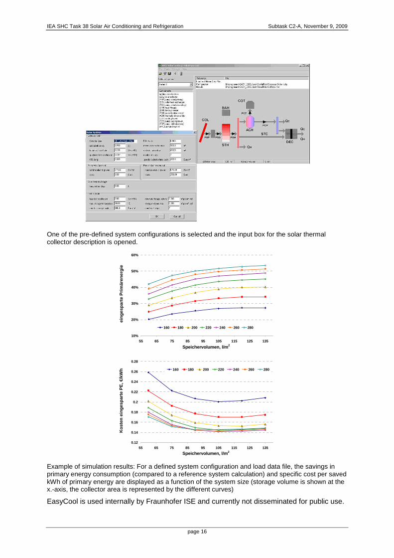
One of the pre-defined system configurations is selected and the input box for the solar thermal collector description is opened.
10%
20%
30%
40%
50%
60%
55 65 75 85 95 105 115 125 135
Speichervolumen, l/m 2
eing
espa
rte
Prim
ären
ergi
e
160 180 200 220 240 260 280
0.12
0.14
0.16
0.18
0.2
0.22
0.24
0.26
0.28
55 65 75 85 95 105 115 125 135
Speichervolumen, l/m 2
Kos
ten
eing
espa
rte
PE
, €/k
Wh
160 180 200 220 240 260 280
Example of simulation results: For a defined system configuration and load data file, the savings in primary energy consumption (compared to a reference system calculation) and specific cost per saved kWh of primary energy are displayed as a function of the system size (storage volume is shown at the x.-axis, the collector area is represented by the different curves)
EasyCool is used internally by Fraunhofer ISE and currently not disseminated for public use.

IEA SHC Task 38 Solar Air Conditioning and Refrigeration Subtask C2-A, November 9, 2009
page 17
INSEL Antoine Dalibard ZAFH.NET (Stuttgart University of Applied Sciences) The acronym INSEL stands for INtegrated Simulation Environment Language. This graphical programming language has been developed at the Faculty of Physics of Oldenburg University (Germany) in the early 1990’s and was originally designed for the modelling of renewable electrical energy systems. Today INSEL covers the whole range of renewable energy systems, including building simulation and communication technologies. The software can be adapted by the user for completely own software developments and offers a transparent software solution from the planning phase to automation and simulation based control of any energy plants. Basic idea of INSEL The graphical programming language INSEL is based on the principle of “structured programming” on blocks diagrams. It consists of connecting blocks in order to obtain block diagrams that express a solution for a certain simulation task. Application areas of INSEL The main application areas of the program INSEL are:
• Energy meteorology
• Photovoltaic systems
• Solar thermal systems
• Solar thermal power plants
• Building simulation (under development)
• Building automation (under development)
• Facility management (under development) Main uses of INSEL INSEL is a block diagram simulator that can be used by researchers, planers, designers, operators and investors for:
• Design of complex energy systems
• Visualisation and Internet monitoring
• Monitoring and control of energy plants
• Highly precise yield prognoses and economic calculations of energy systems.

IEA SHC Task 38 Solar Air Conditioning and Refrigeration Subtask C2-A, November 9, 2009
page 18
Structure of the program The different layers of INSEL are:
Graphical Interface : HP-VEE panel view
Graphical simulation model (file .vee) Text simulat ion model (file .ins)
Data bases (weather, components,…)
INSEL compiler: inselEngine.dll
Execution: inselDi.dll
Interfaces: call of the conventions, header
Blocks implementation
INSEL block concept
Additional Information:
• INSEL main window:
• Graphical Interface: HP-VEE is used as graphical interface
• Source code of the models: not available
Assign a file to compile
Open block diagram editor
Open GnuPlot
Open text editor
Open SunOrb
Open InselWeather data
browser
Open MSDOS command
Open calculator

IEA SHC Task 38 Solar Air Conditioning and Refrigeration Subtask C2-A, November 9, 2009
page 19
• Modularity: since INSEL is a programming language, it is entirely modular. It is possible to define any energetic systems.
• Time steps increment: any time steps can be defined from less than 1sec to several years.
• Components library extension: It is possible to write source code in Fortran and C++ and to create new components in order to extend the components library by linking the code to a dynamic link library DLL.
• Meteorological databases used: INSEL database (2000 locations worldwide), European solar radiation Atlas, Meteonorm, S@tel light plus any other source available.
Components library The main components of INSEL related to solar thermal application and solar cooling in particular are:
• Collectors: dynamic models of air and liquids collectors
• Storage tanks: fully mixed and stratified models
• Heat exchangers: simple models (parallel, counter and cross flows), cross flow heat exchanger with condensing and icing, earth heat exchanger (under development).
• Desiccant wheel
• Absorption chillers: models for Phönix (10 kW) and EAW (from 15 to 200 kW) chillers.
• Adsorption chillers: dynamic model under development.
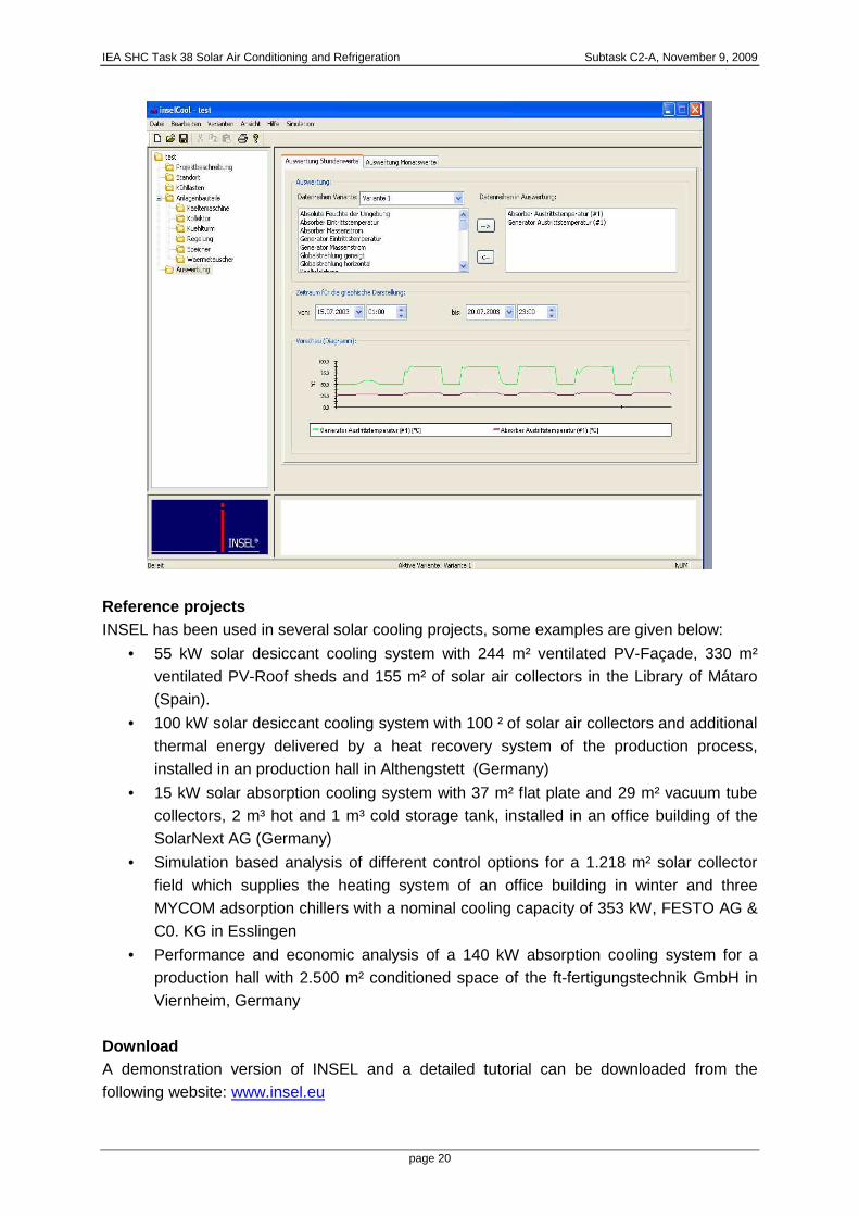
• Cooling towers: open-wet model A specific application for solar cooling: INSEL Coo l An application for solar cooling (INSEL Cool) has been implemented into INSEL in order to help planners during the pre-design phase of a solar cooling plant. Users have the possibility to perform simulation of solar cooling installing by selecting in a list the main components of the installation (cooling machines, solar collectors, cooling towers, storage tanks, heat exchangers), the location of the installation and the cooling load profile. It is also possible to define new components and new locations by introducing himself the required parameters and external cooling load files can be used for simulation. The analysis of the results can be done (either with hourly or monthly values) directly from the application as can be seen in the figure below.
IEA SHC Task 38 Solar Air Conditioning and Refrigeration Subtask C2-A, November 9, 2009
page 20
Reference projects INSEL has been used in several solar cooling projects, some examples are given below:
• 55 kW solar desiccant cooling system with 244 m² ventilated PV-Façade, 330 m² ventilated PV-Roof sheds and 155 m² of solar air collectors in the Library of Mátaro (Spain).
• 100 kW solar desiccant cooling system with 100 ² of solar air collectors and additional thermal energy delivered by a heat recovery system of the production process, installed in an production hall in Althengstett (Germany)
• 15 kW solar absorption cooling system with 37 m² flat plate and 29 m² vacuum tube collectors, 2 m³ hot and 1 m³ cold storage tank, installed in an office building of the SolarNext AG (Germany)
• Simulation based analysis of different control options for a 1.218 m² solar collector field which supplies the heating system of an office building in winter and three MYCOM adsorption chillers with a nominal cooling capacity of 353 kW, FESTO AG & C0. KG in Esslingen
• Performance and economic analysis of a 140 kW absorption cooling system for a production hall with 2.500 m² conditioned space of the ft-fertigungstechnik GmbH in Viernheim, Germany
Download A demonstration version of INSEL and a detailed tutorial can be downloaded from the following website: www.insel.eu

IEA SHC Task 38 Solar Air Conditioning and Refrigeration Subtask C2-A, November 9, 2009
page 21
Chapter II: New developments in simulations tools a nd models A solar desiccant cooling installation model in SPA RK, A transient detailed model of the desiccant wheel. Paul Bourdoukan LOCIE FRE CNRS 3220, Institut National de l'Energie Solaire (INES), Etienne Wurtz LOCIE FRE CNRS 3220, Institut National de l'Energie Solaire (INES),
The present chapter presents a modelling approach of a solid desiccant air handling unit
powered by vacuum tube solar collectors. It is divided into 3 sections.
In section (1) the model of the installation is described by separately considering each
component (i.e. sensible heat regenerator, desiccant wheel, evaporative coolers, solar
collectors, storage tank).
In the section (2) an experimental validation of the presented model is performed under
different operating conditions on a component level and on a system level.
Section (3) is dedicated for a transient model of the desiccant wheel. Unlike conventional
models that give a mean temperature and a mean humidity ratio at the outlet of the wheel
this detailed transient model gives the temperature and humidity profile at the outlet of the
wheel. The model is then validated experimentally.
The presented models with the experimental validation are a summary of different research
work [1], [2], [3], [4] and [5] published recently and highlighted in the reference section.

IEA SHC Task 38 Solar Air Conditioning and Refrigeration Subtask C2-A, November 9, 2009
page 22

IEA SHC Task 38 Solar Air Conditioning and Refrigeration Subtask C2-A, November 9, 2009
page 23
1. Modelling of the solar desiccant cooling installation
A model implementation of a desiccant cooling installation powered by vacuum tube solar
collectors in SPARK is described in this section. The Desiccant wheel, the sensible
regenerator and the evaporative cooler are selected from bibliography. However a new
developed model of the vacuum heat pipe solar colle ctors is presented.
The aim of this implementation is to predict accurately the supply conditions of a desiccant
air handling for different operating conditions and to predict the real potential of solar energy
in this process.
Nomenclature
Symbols
cpa heat capacity of air [J.kg-1.K-1]
cpv heat capacity of water vapor [J.kg-1.K-1]
cpm heat capacity of the regenerator matrix [J.kg-1.K-1]
Cmin min capacitance rate of the regenerator inlet fluids [J.s-1.K-1]
Cr parameter used in the correlation of the regenerator [-]
e thickness [m]
Fi potential characteristic [-]
G solar global radiation [W. m-2]
h heat transfer coefficient [W.K-1m-2]
ha enthalpy of moist air [J.Kg-1]
hfg latent heat of vaporization [J.kg]
H enthalpy of the sensible or desiccant regenerator matrix [J.Kg-1]
Jt lumped heat transfer coefficient [s-1]
Jm lumped mass transfer coefficient [s-1]
K heat loss constant [W.K-1m-2]
L width of the desiccant wheel [m]
Lv latent heat of vaporization of the heat pipe fluid [J.kg-1]
Le Lewis number [-]
ma air mass flow rate [Kg.s-1]
M mass [kg]
Md mass of the desiccant matrix [Kg]
Mm mass of the aluminium matrix [Kg]
N angular speed of the wheel [rd.s-1]
Na number of nodes in the angular direction of the desiccant wheel [-]
Np number of nodes in the width direction of the desiccant wheel [-]

IEA SHC Task 38 Solar Air Conditioning and Refrigeration Subtask C2-A, November 9, 2009
page 24
NTU number of transfer unit [-]
S area [m2]
t time [s]
Ta air temperature [K]
Teq equilibrium temperature [K]
Ti air temperature in the section i (i=1;9) [K]
Tm matrix temperature [K]
u fluid velocity (m.s-1)
V volume (m3)
wa humidity ratio of moist air. [Kg.Kg-1dryair]
Wd water content of desiccant [Kg.Kg-1desiccant]
x variable [arbitrary]
z coordinate in the fluid flow direction [m]
Greek letters
ε emissivity [dimensionless]
γi parameter used in the reduction of desiccant wheel equations [-]
∆λ parameter in the desiccant enthalpy [-]
µ ratio of matrix mass over air mass [-]
ηcf efficiency of the counter flow heat exchanger [-]
τα transmission-absorptance coefficient
σ Stefan Boltzmann constant [W.K-4m-2]
ρ density [kg.m-3]
λ conductivity [W.K-1m-1]
τro half period of rotation of the desiccant wheel [s]
θ cylindrical coordinate or angular position [rd]
Subscripts
a air
b buffer
c condenser
d desiccant
eq equilibrium
f fluid
g glass
i inlet
H heat pipe

IEA SHC Task 38 Solar Air Conditioning and Refrigeration Subtask C2-A, November 9, 2009
page 25
m matrix (sensible regenator)
p plate absorber
o outlet
reg regeneration
sat saturation
Desiccant cooling principle
A desiccant cooling installation operating under the conventional configuration (100% air-
change rate), with corresponding changes in the air properties in the psychometric chart, is
shown in Figure 1.
Figure 1: Desiccant cooling system with correspondi ng evolution of air properties in the
psychometric chart
6
Evaporative coolers
7 8 9
Regeneration Heat
exchanger
Collectors
Heat exchanger
Building
1
i
n
m2 T1
m1 Tn
m1 Ti1
m2 Ti2
Buffer
Sensible heat regenerator
5
3 way valve
4 3 2 1
Desiccant wheel

IEA SHC Task 38 Solar Air Conditioning and Refrigeration Subtask C2-A, November 9, 2009
page 26
With reference to Figure 1, the conventional cycle operates as follows: outside air (1) is
dehumidified in a desiccant wheel (2); it is then cooled in the sensible regenerator (3) by the
return cooled air before undergoing another cooling stage by evaporation (4) and being
introduced into the building. The operating sequence for the return air (5) is as follows: it is
cooled to its saturation temperature by evaporative cooling (6) and then it cools the fresh air
in the rotary heat exchanger (7). It is then heated in the regeneration heat exchanger by solar
energy (8), it regenerates the desiccant wheel (9) by removing the humidity and exits the
installation.
Modelling of the components
Sensible regenerator
A sensible regenerator is a porous matrix which passes periodically between a hot and a
cold stream. The cellular matrix of the regenerator stores heat from the hot gas stream and
releases it to the cold gas stream.
Figure 2: Sensible heat regenerator principle
For modelling purposes, the following assumptions are made:
• Heat transfer between air and the regenerator matrix is considered using a lumped
transfer coefficient or a number of transfer units (NTU)
• The channels where the fluid flows are identical and parallel
• No leakage occurs between the air streams
The heat conservation and transfer governing equations, after Kays and London [6] and
Maclaine-cross and Banks [7], are:
Hot air stream
Cold air stream
T2
T3
T6
Cooled air stream
Heated air stream
T7

IEA SHC Task 38 Solar Air Conditioning and Refrigeration Subtask C2-A, November 9, 2009
page 27
0=∂
∂+
+∂
∂+∂
∂t
Tm
cwc
c
z
Tau
t
Ta
pvapa
pmµ (1)
0)( , =−+∂
∂+ amat
pvapa
pm TTJt
Tm
cwc
cµ (2)
Kays and London [6] proposed the following correlation for regenerator efficiency (RE):
( )
−=
93.1*9
11
r
cfC
RE η (3)
Where:
min
* ..
C
NcMC pmm
r = (4)
cf
cfcf NTU
NTU
+=
1η (5)
is the efficiency of the counter-flow heat exchanger for balanced flow.
The outlet temperature (T3) of the sensible regenerator can thus be calculated using:
62
32
TT
TTRE
−−= (6)
Desiccant wheel
The wheel is divided into two sectors the first is for dehumidification of moist air while the second is for
the regeneration. It is a rotating porous matrix impregnated with a desiccant material that alternates
periodically between a process air stream and a hot air stream. In contact with the dry desiccant,
process air is dehumidified and heated by the heat of adsorption. The saturated desiccant then enters
into contact with the hot air stream and is regenerated to again dehumidify the process air,
perpetuating the dehumidification-regeneration cycle.
The wheel is driven by a small electrical motor, with a rotation speed that varies between 7 and 20 rph

IEA SHC Task 38 Solar Air Conditioning and Refrigeration Subtask C2-A, November 9, 2009
page 28
Figure 3: Desiccant wheel
The desiccant wheel model used below is that proposed first by Banks [8] and also by
Maclaine-cross and Banks [7]. The following assumptions are made [3]:
• The state properties of the air streams are spatially uniform at the desiccant wheel
inlet
• The interstices of the porous medium are straight and parallel
• There is no leakage or carry-over of streams
• The interstitial air velocity and pressure are constant
• Heat and mass transfer between the air and the porous desiccant matrix is
considered using lumped transfer coefficients
• Diffusion and dispersion in the fluid flow direction are neglected
• No radial variation of the fluid or matrix states
• The sorption isotherm does not represent a hysteresis
• Air reaches equilibrium with the porous medium
Heat and mass conservation equations:
0=∂
∂+∂
∂+∂
∂t
H
z
hu
t
h daa µ (7)
0=∂
∂+∂
∂+∂
∂t
W
z
wu
t
w daa µ (8)
Heat and mass transfer equations:
0)())(( ,, =∂∂−+
∂∂−+
∂∂
Ta
aaeqa
wa
aaeqam
d
w
hww
T
hTTLeJ
t
Hµ (9)
0)( , =−+∂
∂aeqam
d wwJt
Wµ (10)
Outside moist air
Dry air
Regeneration hot air Exhaust
humid air

IEA SHC Task 38 Solar Air Conditioning and Refrigeration Subtask C2-A, November 9, 2009
page 29
Equations (7), (8), (9) and (10) are coupled, hyperbolic and non-linear. With the assumption
of the Lewis number (Le), equal unity and the desiccant matrix in equilibrium with air means
that (Td= Teq and weq= wa). Banks [8] used matrix algebra and demonstrated that these
equations (7 to 10) can be reduced by applying the potential function Fi(T,w) to the following
system:
0,,, =∂
∂+
∂∂
+∂
∂z
F
t
Fu
t
F aiaieqii µγ i=1;2 (11)
0)( ,,, =−+
∂∂
aieqimdi
i FFJt
Fµγ i=1;2 (12)
These equations are similar to those for the sensible regenerator (Equations 1 and 2), with
the potential function Fi replacing the temperature and the parameters γi replacing the
specific heat ratio, and they can be solved using analogy with heat transfer alone as
suggested by Maclaine-cross and Banks [7] and Close and Banks [9]. There are many
expressions for the potential functions of moist air-silica gel; we chose those proposed by
Jurinak [10] and Stabat [11].
hF =1 (13)
( ) 8.05.1
2 1.16360
15.273w
TF ++= (14)
The solution sequence for the desiccant wheel is then:
j
aij mC
.
=
)(min.
* moyij
a
dri
m
NMC γ=
i
i
iC
CC
max
min* =
( ) ( )
1
min0
111−
+=
rmsm AhAhCNUT
( ) ( )
−=
93.1*09
11,
ri
im
cciC
CNUTεε or *rii C=ε ( 4.0* ≤riC ) for very low rotation speed
IEA SHC Task 38 Solar Air Conditioning and Refrigeration Subtask C2-A, November 9, 2009
page 30
For the desiccant wheel the efficiency is written with the potential functions instead of
temperatures for the sensible regenerator:
(With Fi,k where the subscript i indicates the potential and the subscript k indicates the
position relatively to figure 1)
1,18,1
1,12,11min
1
1 FF
FF
C
Cn
−−
=ε
1,28,2
1,22,22min
2
2 FF
FF
C
Cn
−−
=ε
To calculate the outlet conditions of the regeneration stream the conservation equations are
applied to the potential functions:
( ) ( )8,19,11
1,12,11 FFCFFC rn −=−
( ) ( )8,29,22
1,22,22 FFCFFC rn −=−
Having the potential functions calculated the temperature and humidity ratio at both outlet of
the wheel can thus be calculated
Evaporative coolers
The humidification process occurs at a constant wet-bulb temperature. During the process,
the energy needed for droplet evaporation is taken from the air which yields its temperature
decrease and humidity increase. The enthalpy of the moist air at the evaporative cooler inlet
is the sum of the enthalpy of the dry air and that of the water vapor. At the evaporator cooler
outlet; the enthalpy of the dry air decreases due to the temperature decrease while that of
water vapor increases due to the increased water vapor mass but the total enthalpy of moist
air is approximately constant, with a slight increase due to the addition of the enthalpy of
liquid water droplets.
outletainleta wThwTh ,, ),(),( = (15)
The validity of this assumption can be verified on the psychometric chart where the lines of
constant wet-bulb temperature are parallel to the constant enthalpy lines, especially when
the temperature and humidity ratio are, respectively, between 19 and 25°C and 7 and
15g/Kg, which is in the application domain of desiccant evaporative cooling.
IEA SHC Task 38 Solar Air Conditioning and Refrigeration Subtask C2-A, November 9, 2009
page 31
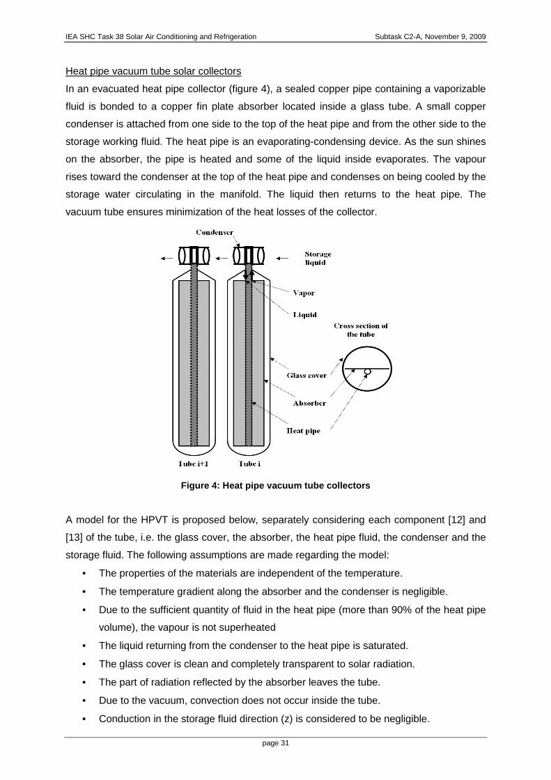
Heat pipe vacuum tube solar collectors
In an evacuated heat pipe collector (figure 4), a sealed copper pipe containing a vaporizable
fluid is bonded to a copper fin plate absorber located inside a glass tube. A small copper
condenser is attached from one side to the top of the heat pipe and from the other side to the
storage working fluid. The heat pipe is an evaporating-condensing device. As the sun shines
on the absorber, the pipe is heated and some of the liquid inside evaporates. The vapour
rises toward the condenser at the top of the heat pipe and condenses on being cooled by the
storage water circulating in the manifold. The liquid then returns to the heat pipe. The
vacuum tube ensures minimization of the heat losses of the collector.
Figure 4: Heat pipe vacuum tube collectors
A model for the HPVT is proposed below, separately considering each component [12] and
[13] of the tube, i.e. the glass cover, the absorber, the heat pipe fluid, the condenser and the
storage fluid. The following assumptions are made regarding the model:
• The properties of the materials are independent of the temperature.
• The temperature gradient along the absorber and the condenser is negligible.
• Due to the sufficient quantity of fluid in the heat pipe (more than 90% of the heat pipe
volume), the vapour is not superheated
• The liquid returning from the condenser to the heat pipe is saturated.
• The glass cover is clean and completely transparent to solar radiation.
• The part of radiation reflected by the absorber leaves the tube.
• Due to the vacuum, convection does not occur inside the tube.
• Conduction in the storage fluid direction (z) is considered to be negligible.

IEA SHC Task 38 Solar Air Conditioning and Refrigeration Subtask C2-A, November 9, 2009
page 32
The glass cover exchanges heat by convection with the outside air and by radiation with the
sky and the absorber. The absorber receives solar radiation and heats the fluid inside the
tube. The vapour rising from the heat pipe enters the condenser and releases energy to the
circulating storage fluid, then exits the condenser as a saturated liquid. The heat pipe liquid is
heated to saturation before the evaporation process begins.
The governing equations for each component (characterized by heat capacity C and
temperature T):
Glass cover:
)()()( 4444gagggpppgskygg
ggg TThSTTSTTS
dt
dTCM −+−+−= σεσε (16)
Absorber:
)()( 44psatHHppgpp
ppp TThSSGTTS
dt
dTCM −++−= τασε (17)
Vapour flow rate:
)( satpHHv TThSLm −= (18)
Condenser:
)()( cfccvvc
cc TThSLmdt
dTCM −+= (19)
Storage fluid:
)()(1 fcccff
f TThSz
Tu
t
TCm −=
∂∂
+∂
∂ (20)
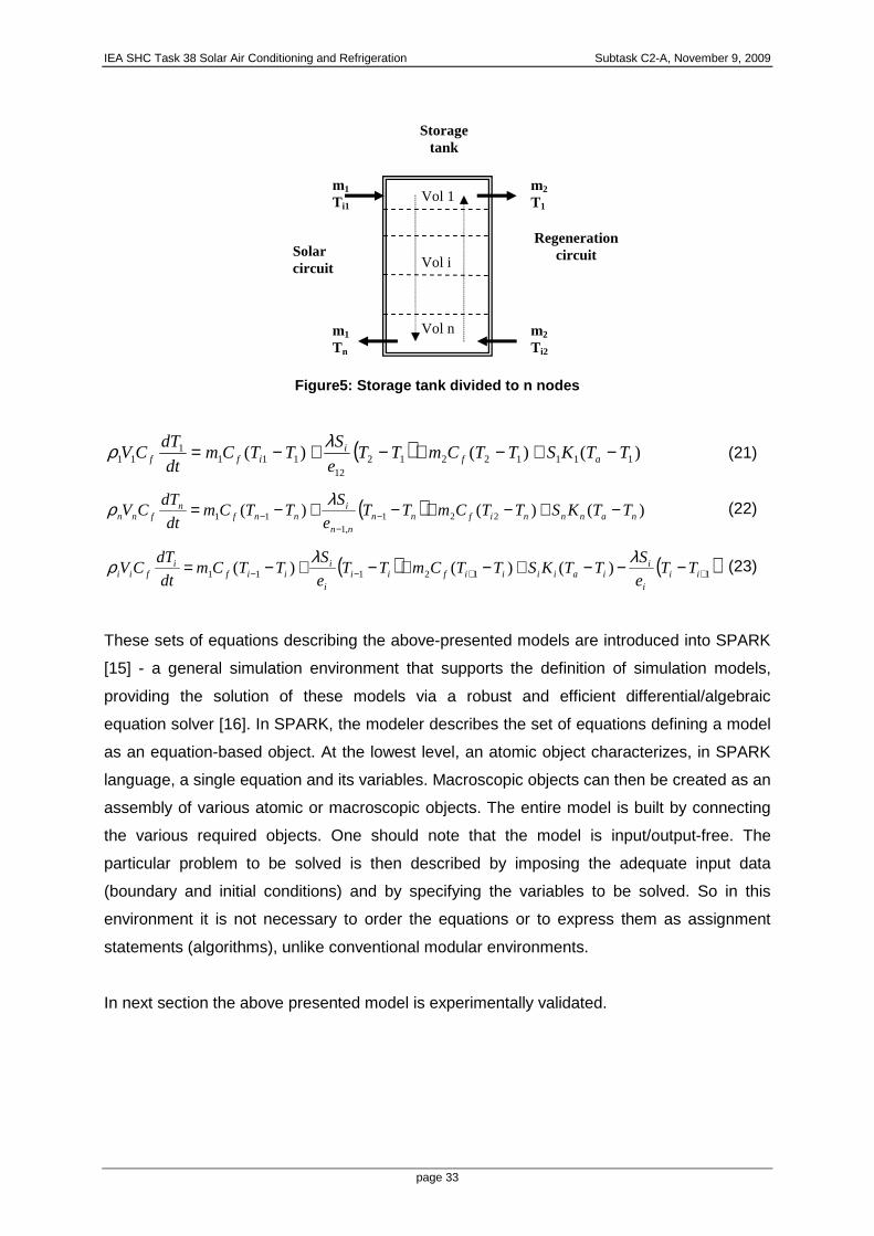
Storage tank
In order to take into account thermal stratification in the storage tank, it is divided into n
nodes [14]. The following equations apply to the first node, the last node (n=12) and the ith
current node:
IEA SHC Task 38 Solar Air Conditioning and Refrigeration Subtask C2-A, November 9, 2009
page 33
Figure5: Storage tank divided to n nodes
( ) )()()( 1111221212
1111
11 TTKSTTCmTTe
STTCm
dt
dTCV af
iiff −+−+−+−= λρ (21)
( ) )()()( 221,1
11 nannnifnnnn
innf
nfnn TTKSTTCmTT
e
STTCm
dt
dTCV −+−+−+−= −
−−
λρ (22)
( ) ( )112111 )()()( ++−− −−−+−+−+−= iii
iiaiiiifii
i
iiif
ifii TT
e
STTKSTTCmTT
e
STTCm
dt
dTCV
λλρ (23)
These sets of equations describing the above-presented models are introduced into SPARK
[15] - a general simulation environment that supports the definition of simulation models,
providing the solution of these models via a robust and efficient differential/algebraic
equation solver [16]. In SPARK, the modeler describes the set of equations defining a model
as an equation-based object. At the lowest level, an atomic object characterizes, in SPARK
language, a single equation and its variables. Macroscopic objects can then be created as an
assembly of various atomic or macroscopic objects. The entire model is built by connecting
the various required objects. One should note that the model is input/output-free. The
particular problem to be solved is then described by imposing the adequate input data
(boundary and initial conditions) and by specifying the variables to be solved. So in this
environment it is not necessary to order the equations or to express them as assignment
statements (algorithms), unlike conventional modular environments.
In next section the above presented model is experimentally validated.
m2 T1
Vol 1
Vol i
m1 T i1
Vol n m1 Tn
Storage tank
m2 T i2
Solar circuit
Regeneration circuit

IEA SHC Task 38 Solar Air Conditioning and Refrigeration Subtask C2-A, November 9, 2009
page 34
2. Experimental validation
The experimental desiccant installation at La Rochelle [1] was used to validate the model
presented above. The desiccant air handling unit consists of silica gel desiccant wheel, an
aluminum sensible regenerator, two rotating humidifiers, high performance ventilators, a
regeneration heat exchanger (water to air) and an electrical backup used for experimental
purpose. The air handling unit is powered by 40 m2 of heat pipe vacuum tube collectors and
storage tank of 2350 liters.
Psychrometers are used to measure the moist air properties at each section of the air
handling unit (position 1 to 9). Each psychrometer consists of 2 Pt100 sensors: the first
delivers the dry bulb temperature and the second the wet bulb temperature. The local
atmospheric pressure is measured too thus the humidity ratio and relative humidity can be
accurately measured. The temperature of hydraulic system is measured by the means of
Pt100 sensors integrated to the pipes by means of thermo wells. All the Pt100 sensors were
tuned on a temperature range going from 0° to 100°C . The water flow rates are measured
using ultrasonic sensor. The air flow rates were measured using the gas tracer method.In the
difficulty to tune a pyranometer the solar global radiation is measured using two different
pyranometers.
Figure 1 shows a general scheme of the experimental installation. In order to test different
outside operating conditions (to test the models under different conditions) an outside
conditions simulator was coupled to the desiccant air handling unit. The outside conditions
simulator consists of a pre-heater, a humidifier and a heater, this permits the test at high
temperatures and high humidity ratio.
The cooling load on the installation was controlled using load simulator that consists of
heater and replaces the building load. This permitted to control the return conditions during
the tests.
For the model validation different operating were considered for all the components.

IEA SHC Task 38 Solar Air Conditioning and Refrigeration Subtask C2-A, November 9, 2009
page 35
Figure 6: Experimental solar desiccant cooling inst allation of La Rochelle
2 4
5 7 8 9
Desiccant wheel
Sensible regenerator
Regeneration heat exchanger
Humidifiers
Collector Tank
Heater
Humidifier
Heat exchanger
Load simulator
1
Pre heating
Fan
Outside air
Outside conditions simulator
Desiccant air handling unit
Solar installation
Backup 6
Valve
3
Pump

IEA SHC Task 38 Solar Air Conditioning and Refrigeration Subtask C2-A, November 9, 2009
page 36
Experimental validation of components’ model
The sensible regenerator
The outlet temperature of the sensible regenerator depends on the temperature at both inlets
of the regenerator. Various temperature differences between the inlets of the regenerator
(position 2 and 6) were considered. Figure 7 below plots the experimental efficiency of the
regenerator as well as the outlet temperature deviation of the model relative to the
measurements.
0
0.1
0.2
0.3
0.4
0.5
0.6
0.7
0.8
0.9
1
5 10 15 20 25 0
0.1
0.2
0.3
0.4
0.5
0.6
0.7
0.8
0.9
1
Exper
imen
tal
effi
cien
cy [
-]
Tem
per
ature
dev
iati
on [
°C]
Temperature difference (T2-T6) [°C]
Sensible Regenerator
Efficiency
Deviation
Figure 7: experimental efficiency of the sensible r egenerator and deviation of the model
prediction of the outlet temperature with respect t o measurements
Figure 7 shows that the measured efficiency of the sensible regenerator is nearly constant
and equal to 0.7 in all cases; it also shows that the error in predicting the outlet temperature
(position 3 in Figure 1) of the regenerator using the model presented above is low, never
exceeding 0.5°C. It should be noted that this devia tion is in the domain of the accuracy of the
measurements. This accuracy can be predicted, as the efficiency is constant, independent of
the operating temperature.
The desiccant wheel
For the desiccant wheel model, different inlet conditions (position 1 with reference to Figure
1) were considered with the temperature varying from 25°C to 38°C and the humidity ratio
from 10 to 15g/kg, and for different regeneration temperatures (60°C, 65°C, 70°C and 80°C).
Figure 8 plots temperature error against humidity ratio error for the most significant points.

IEA SHC Task 38 Solar Air Conditioning and Refrigeration Subtask C2-A, November 9, 2009
page 37
-3
-2.5
-2
-1.5
-1
-0.5
0
0.5
1
1.5
2
2.5
3
-2 -1.5 -1 -0.5 0 0.5 1 1.5 2
Tem
per
ature
dev
iati
on [
°C]
Humidity ratio deviation [g.kg-1
]
Desiccant wheel
Treg=80 °C
Treg=70 °C
Treg=65 °C
Treg=60 °C
measurement accuarcy
Figure 8: Deviation of the outlet temperature and o utlet humidity ratio in comparison with
measured results for different operating conditions
The maximum error in predicting the temperature at the outlet of the desiccant wheel is 1°C
(a relative error of 2.5%). This error occurs for different regeneration temperatures and for
the same inlet temperature of the wheel, 38°C, whic h is not in the application domain of
desiccant cooling. For the humidity ratio, the maximum error is 0.5 g/kg but it should be
noted that the accuracy of humidity ratio measurement in the air handling unit is 0.4 g/kg (this
accuracy can be tested by comparing the humidity ratio at points 2, 3 and 4 of Figure 1 with
the supply humidifier switched off; in this case the points must have the same humidity ratio),
so the error is in the validity domain of the measurements.
This accuracy of the model is obtained when the mod el is dynamically parameterized
in function of the operating regeneration temperatu re; if this is not the case, the
deviation will be more significant when the operati ng regeneration temperature is
much higher than that of rating conditions used to parameterize the model [1].
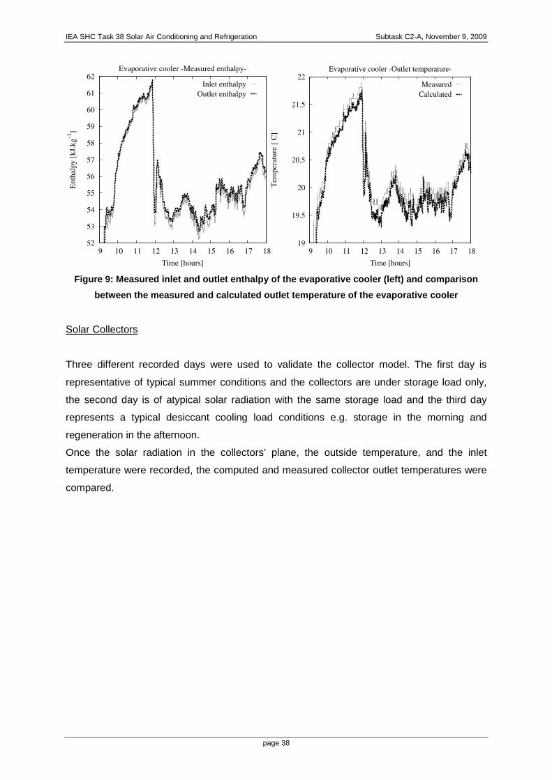
The evaporative cooler
For the evaporative cooler model, Figure 9 demonstrates that the enthalpy is constant across
the evaporative cooler and that the constant enthalpy model can thus accurately predict the
outlet temperature of the evaporative cooler.
IEA SHC Task 38 Solar Air Conditioning and Refrigeration Subtask C2-A, November 9, 2009
page 38
52
53
54
55
56
57
58
59
60
61
62
9 10 11 12 13 14 15 16 17 18
Enth
alpy [
kJ.
kg
-1]
Time [hours]
Evaporative cooler -Measured enthalpy-
Inlet enthalpy
Outlet enthalpy
19
19.5
20
20.5
21
21.5
22
9 10 11 12 13 14 15 16 17 18
Tem
pera
ture
[°C
]
Time [hours]
Evaporative cooler -Outlet temperature-
Measured
Calculated
Figure 9: Measured inlet and outlet enthalpy of the evaporative cooler (left) and comparison
between the measured and calculated outlet temperat ure of the evaporative cooler
Solar Collectors
Three different recorded days were used to validate the collector model. The first day is
representative of typical summer conditions and the collectors are under storage load only,
the second day is of atypical solar radiation with the same storage load and the third day
represents a typical desiccant cooling load conditions e.g. storage in the morning and
regeneration in the afternoon.
Once the solar radiation in the collectors’ plane, the outside temperature, and the inlet
temperature were recorded, the computed and measured collector outlet temperatures were
compared.

IEA SHC Task 38 Solar Air Conditioning and Refrigeration Subtask C2-A, November 9, 2009
page 39
Day 1:
0
100
200
300
400
500
600
700
800
900
1000
0 100 200 300 400 500
Radia
tion [
W.m
-2]
Time [min]
Solar global radiation -Day 1-
30
40
50
60
70
80
90
0 100 200 300 400 500T
emp
erat
ure
[°C
]Time [min]
Outlet temperature -Day 1-
Experimental
Model
Figure 10: comparison of the predicted outlet tempe rature of the collectors with the measured
one for perfect radiation conditions and a storage load
Comparison between the computed and the measured temperatures for the typical summer
day conditions shows the model’s high performance in predicting collector outlet temperature
with a negligible error. This accuracy is due to the fact that each component is taken into
consideration by the model and the calculations are performed in each vacuum tube
simultaneously (400 tubes).
While collector outlet temperature can thus be predicted accurately in normal radiation
conditions, it is very important to study the performance of the model for atypical conditions.
Day 2:
0
100
200
300
400
500
600
700
800
900
1000
1100
1200
0 100 200 300 400 500
Radia
tion [
W.m
-2]
Time[min]
Solar global radiation -Day 2-
60
70
80
90
100
0 100 200 300 400 500
Tem
per
ature
[°C
]
Time [min]
Outlet temperature -Day 2-
Experimental
Model
Figure 11: comparison of the predicted outlet tempe rature of the collectors with the measured
one for fluctuating radiation conditions and a stor age load
IEA SHC Task 38 Solar Air Conditioning and Refrigeration Subtask C2-A, November 9, 2009
page 40
By comparing the calculated and the measured outlet temperatures for the atypical
conditions day, when the overall solar radiation fluctuated constantly, it can be seen that the
model very accurately predicts the outlet temperature for the whole day, whatever the
amplitude of the solar radiation fluctuations and the maximum error is always below 2°C but
the model does not show any time delay with respect to the measurments.
In these first two cases, the model correctly predicts the collector outlet temperature under
different radiation conditions but for storage load. The next step in the validation procedure is
to study the model’s response to a desiccant cooling load, i.e. storage in the morning, with
regeneration in the afternoon.
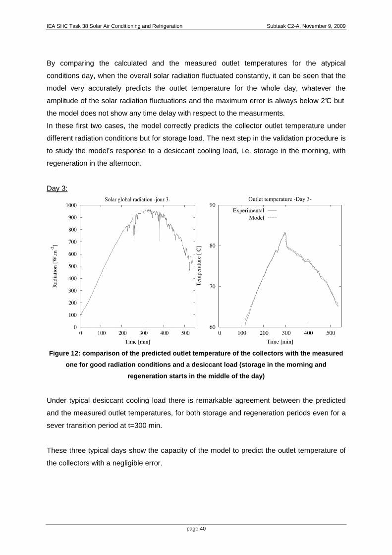
Day 3:
0
100
200
300
400
500
600
700
800
900
1000
0 100 200 300 400 500
Rad
iati
on
[W
.m-2
]
Time [min]
Solar global radiation -jour 3-
60
70
80
90
0 100 200 300 400 500
Tem
per
atu
re [
°C]
Time [min]
Outlet temperature -Day 3-
Experimental
Model
Figure 12: comparison of the predicted outlet tempe rature of the collectors with the measured
one for good radiation conditions and a desiccant l oad (storage in the morning and
regeneration starts in the middle of the day)
Under typical desiccant cooling load there is remarkable agreement between the predicted
and the measured outlet temperatures, for both storage and regeneration periods even for a
sever transition period at t=300 min.
These three typical days show the capacity of the model to predict the outlet temperature of
the collectors with a negligible error.

IEA SHC Task 38 Solar Air Conditioning and Refrigeration Subtask C2-A, November 9, 2009
page 41
Storage Tank
Two different scenarios are considered for the validation of the storage tank model. In the
first only storage is considered (m1>0 and m2=0 in reference to Figure 5) while for the second
it concerns desiccant cooling application with storage in the morning and regeneration in the
afternoon (m1>0 and m2>0). The flow rates m1 and m2 are measured as well as the inlet
temperature of the storage tank. The predicted and measured temperatures at the top and
the bottom of the buffer are compared in the Figure 13 below.
0
10
20
30
40
50
60
70
80
90
0 100 200 300 400
Tem
per
ature
[°C
]
Time [min]
Storage load
Top experimental
Top model
Bottom experimental
Bottom model 0
10
20
30
40
50
60
70
80
90
0 100 200 300 400
Tem
per
ature
[°C
]
Time [min]
Typical desiccant load
Top experimental
Top model
Bottom experimental
Bottom model
Figure 13: Comparison of the predicted temperature with measured one for the top and the
bottom of the storage tank under a storage load (le ft) and a desiccant load (right)
In both scenarios the model can accurately predict the temperature at the top and the bottom
of the buffer. In the first case the stratification remains fairly constant but increases when the
storage and the regeneration are combined. This may at first, appear incoherent as more
mixing occurs in the latter case. The fact that stratification is greater with the regeneration is
that the regeneration load was applied by water loss and the return water was cold and
significantly below the tank temperature which amplified the stratification. Even with this
extreme case the model was capable to predict accurately the temperature at the top and the
bottom of the buffer.
Now if the model has shown an acceptable accuracy when considered solely, we have to be
sure that this accuracy will not be lost when coupling the components making the numerical
simulation useless. In the next section the error propagation will be analysed and the impact
on the supply temperature is examined.

IEA SHC Task 38 Solar Air Conditioning and Refrigeration Subtask C2-A, November 9, 2009
page 42
Error propagation
For the solar installation the maximum error in the temperature prediction was that of the
tank with a maximum error of 1°C which yields an er ror in the prediction of the regeneration
temperature. Or the experimental results showed that 1°C difference in the regeneration
temperature does not have any practical impact on the performance of the desiccant wheel
and thus on the supply conditions.
For the air handling unit the evaporative cooler model and the sensible regenerator models
has shown negligible errors. In reversal the desiccant wheel model has shown simultaneous
error in temperature and humidity. Let us consider an error α in the prediction of the outlet
temperature T2 of the desiccant wheel.
The temperature T3 at the outlet of the sensible regenerator in function the inlet temperature
T2 and T6 of the regenerator and its efficiency η:
623 )1( TTT ηη +−= (24)
With the error α in the prediction of the temperature T2 the temperature T3 is now:
)1(3'
3 ηα −+= TT (25)
This means that an error α in the prediction of the T2 will yield an error (1-α) in the prediction
of T3. Now considering an error β in the prediction of the humidity ratio at the outlet of the
wheel, this will yield an error at the outlet temperature of the evaporator cooler in the order
of:
pa
fg
c
hT
β=∆ (26)
hfg is the latent heat of vaporization of water.
With a maximum deviation of 2°C and 0.4 g/kg in the temperature and humidity prediction at
the outlet of the desiccant wheel and appropriately combining the impact of the errors we
have a maximum error of 1.3°C in the prediction of the supply temperature. This is the
maximum error in the supply temperature that can be committed by the model.
Finlay we will compare the overall model prediction for the air handling unit coupled with the
solar installation for day under typical desiccant operations.
IEA SHC Task 38 Solar Air Conditioning and Refrigeration Subtask C2-A, November 9, 2009
page 43
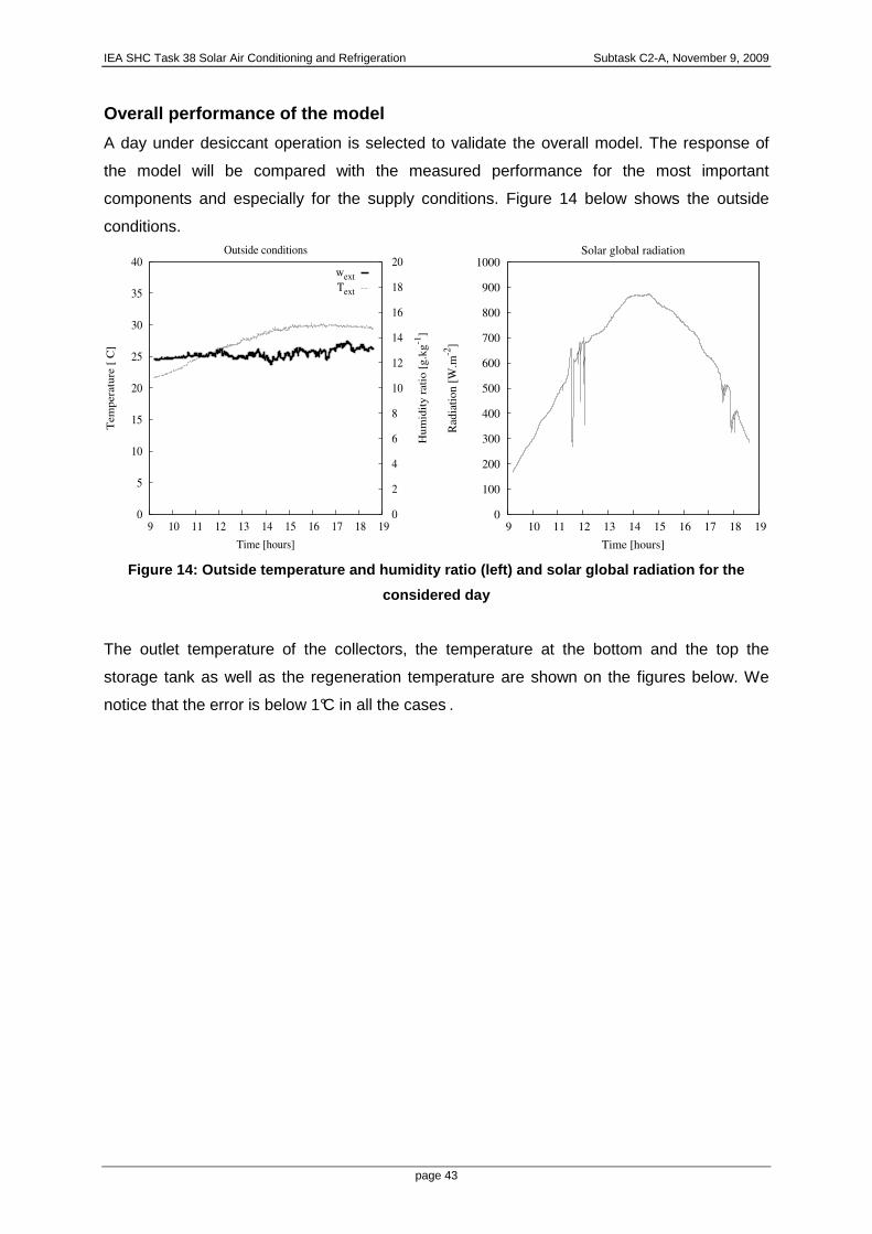
Overall performance of the model
A day under desiccant operation is selected to validate the overall model. The response of
the model will be compared with the measured performance for the most important
components and especially for the supply conditions. Figure 14 below shows the outside
conditions.
0
5
10
15
20
25
30
35
40
9 10 11 12 13 14 15 16 17 18 19 0
2
4
6
8
10
12
14
16
18
20
Tem
pera
ture
[°C
]
Hu
mid
ity
rati
o [
g.k
g-1
]
Time [hours]
Outside conditions
wext
Text
0
100
200
300
400
500
600
700
800
900
1000
9 10 11 12 13 14 15 16 17 18 19
Rad
iati
on [
W.m
-2]
Time [hours]
Solar global radiation
Figure 14: Outside temperature and humidity ratio ( left) and solar global radiation for the
considered day
The outlet temperature of the collectors, the temperature at the bottom and the top the
storage tank as well as the regeneration temperature are shown on the figures below. We
notice that the error is below 1°C in all the cases .

IEA SHC Task 38 Solar Air Conditioning and Refrigeration Subtask C2-A, November 9, 2009
page 44
50
55
60
65
70
75
12 13 14 15 16 17 18
Tem
per
ature
[°C
]
Time [hours]
Collectors outlet temperature
calculated
measured 50
51
52
53
54
55
56
57
58
59
60
12 13 14 15 16 17 18
Tem
per
ature
[°C
]Time [hours]
Tank bottom temperature
calculated
measured
55
56
57
58
59
60
61
62
63
64
65
12 13 14 15 16 17 18
Tem
per
ature
[°C
]
Time [hours]
Tank top temperature
calculated
measured 50
51
52
53
54
55
56
57
58
59
60
12 13 14 15 16 17 18
Tem
per
ature
[°C
]
Time [hours]
Regeneration temperature
calculated
measured
Figure 15: Comparison of the predicted temperature with the measured one for the collectors
outlet, storage top, storage bottom, and regenerati on air
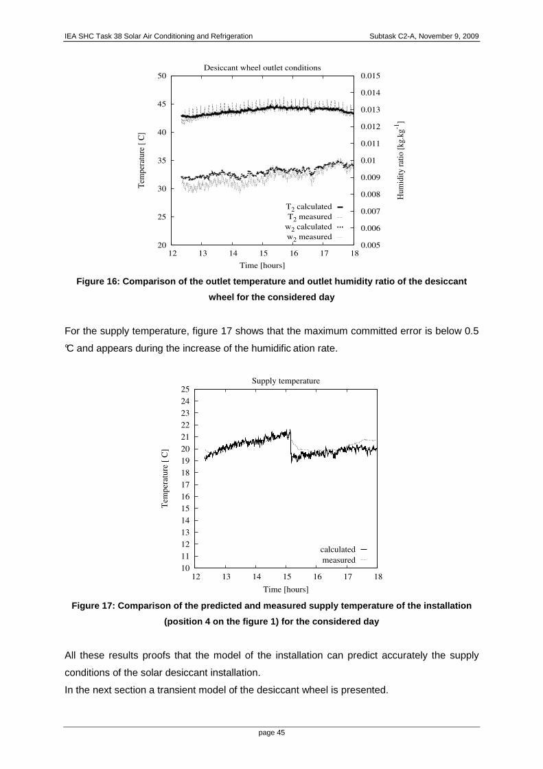
Figure 16 compares the measured outlet conditions of the desiccant wheel to those predicted
by the model. The profiles of the temperature and humidity ratio are very well predicted by
the model during the whole day. For the measured temperature we noticed some peaks et
we can count 7 peaks per hour and for each peak in the temperature corresponds a
minimum in the outlet humidity of the wheel. Or the angular speed of the wheel is 7 rounds
per hour this mean for each revolution of the wheel corresponds a peak. The reason behind
this behaviour is a probable anomaly in the desiccant wheel with a sector having more
desiccant and yields more dehumidification this mean an increase in the outlet temperature
of the wheel. It is evident that the desiccant does not take into account this anomaly.
IEA SHC Task 38 Solar Air Conditioning and Refrigeration Subtask C2-A, November 9, 2009
page 45
20
25
30
35
40
45
50
12 13 14 15 16 17 18 0.005
0.006
0.007
0.008
0.009
0.01
0.011
0.012
0.013
0.014
0.015
Tem
per
ature
[°C
]
Hum
idit
y r
atio
[kg.k
g-1
]
Time [hours]
Desiccant wheel outlet conditions
T2 calculated
T2 measured
w2 calculated
w2 measured
Figure 16: Comparison of the outlet temperature and outlet humidity ratio of the desiccant
wheel for the considered day
For the supply temperature, figure 17 shows that the maximum committed error is below 0.5
°C and appears during the increase of the humidific ation rate.
10
11
12
13
14
15
16
17
18
19
20
21
22
23
24
25
12 13 14 15 16 17 18
Tem
per
ature
[°C
]
Time [hours]
Supply temperature
calculated
measured
Figure 17: Comparison of the predicted and measured supply temperature of the installation
(position 4 on the figure 1) for the considered day
All these results proofs that the model of the installation can predict accurately the supply
conditions of the solar desiccant installation.
In the next section a transient model of the desiccant wheel is presented.

IEA SHC Task 38 Solar Air Conditioning and Refrigeration Subtask C2-A, November 9, 2009
page 46
3. Transient model of the desiccant wheel and experimental validation
Conventional models of the desiccant wheel predict a mean temperature and a mean
humidity ratio at the outlet of the desiccant wheel. In reality and due to the low rotation speed
of the desiccant wheel, the temperature and humidity distribution at the outlet is not uniform.
The model presented in this section is a two dimensional model that gives the temperature
and humidity evolution across the wheel and at its outlets.
Model description
The desiccant wheel scheme is given in the figure below
Figure 18: Schematic of the desiccant wheel
In the model development the following assumption are taken:
• The state properties of the air streams are spatially uniform at the desiccant wheel
inlet
• The interstices of the porous medium are straight and parallel
• There is no leakage or carry-over of streams
• The interstitial air velocity and pressure are constant
• Heat and mass transfer between the air and the porous desiccant matrix is
considered using lumped transfer coefficients
• Diffusion and dispersion in the fluid flow direction are neglected
• No radial variation of the fluid or matrix states
θ
L
Regeneration air
Process air
z
z
R

IEA SHC Task 38 Solar Air Conditioning and Refrigeration Subtask C2-A, November 9, 2009
page 47
A basic element in the angular and width direction of the desiccant wheel is considered and
can be presented as follows:
Figure 19: Basic element of the desiccant wheel
Fundamental equations of heat and mass transfer for the basic element
Mass conservation equation
0=
∂∂+
∂∂+
∂∂
z
wu
t
wm
t
WM aa
ad (27)
Mass transfer equation
( )eqamd wwSht
WM −=
∂∂
(28)
Heat conservation equation
0=
∂∂+
∂∂+
∂∂
z
hu
t
hm
t
HM aa
ad (29)
Heat transfer equation
( )( ) ( )datapvfgeqamd TTShTchwwSht
HM −++−=
∂∂
(30)
Variable change
The time t is related to the angular position θ with the following equation
πθ
τ=
ro
t so θ
πτ rot = ,
Where τro is the rotation period of the process or regeneration and N is the angular speed of
the wheel.
dθ
dz
R
Air

IEA SHC Task 38 Solar Air Conditioning and Refrigeration Subtask C2-A, November 9, 2009
page 48
The partial derivative of a variable x with respect to time t can be thus written with respect to
the angular position θ following: θτ
π∂∂=
∂∂ x
t
x
ro
This yields the following system:
Mass conservation equation
0=
∂∂+
∂∂+
∂∂
z
wu
wm
WM aa
roa
rod θτ
πθτ
π (31)
Mass transfer equation:
( )eqamro
d wwShW
M −=∂∂
θτπ
(32)
Heat conservation equation
0=
∂∂+
∂∂+
∂∂
z
hu
hm
HM aa
roa
rod θτ
πθτ
π (33)
Heat transfer equation
( )( ) ( )datapvfgeqamro
d TTShTchwwShH
M −++−=∂∂
θτπ
(34)
The obtained equation system is coupled non linear hyperbolic, since the enthalpy of the
moist air and of the desiccant depend on the water content and on the temperature.
In the bibliography the equations were solved by Macalaine-cross, [17] and Stabat, [11] by
neglecting the terms θ∂
∂ aw and
θ∂∂ ah
in front of transport term which yields a simplification of
the equations and of the matrix to be solved. In this work we conserved these terms.
Transformation to a discrete problem and restrictio n to 2 dimensions
The wheel is divided into elementary domains following the figure below
∆z
∆θ
R
Figure 20 : discretisation of the desiccant wheel
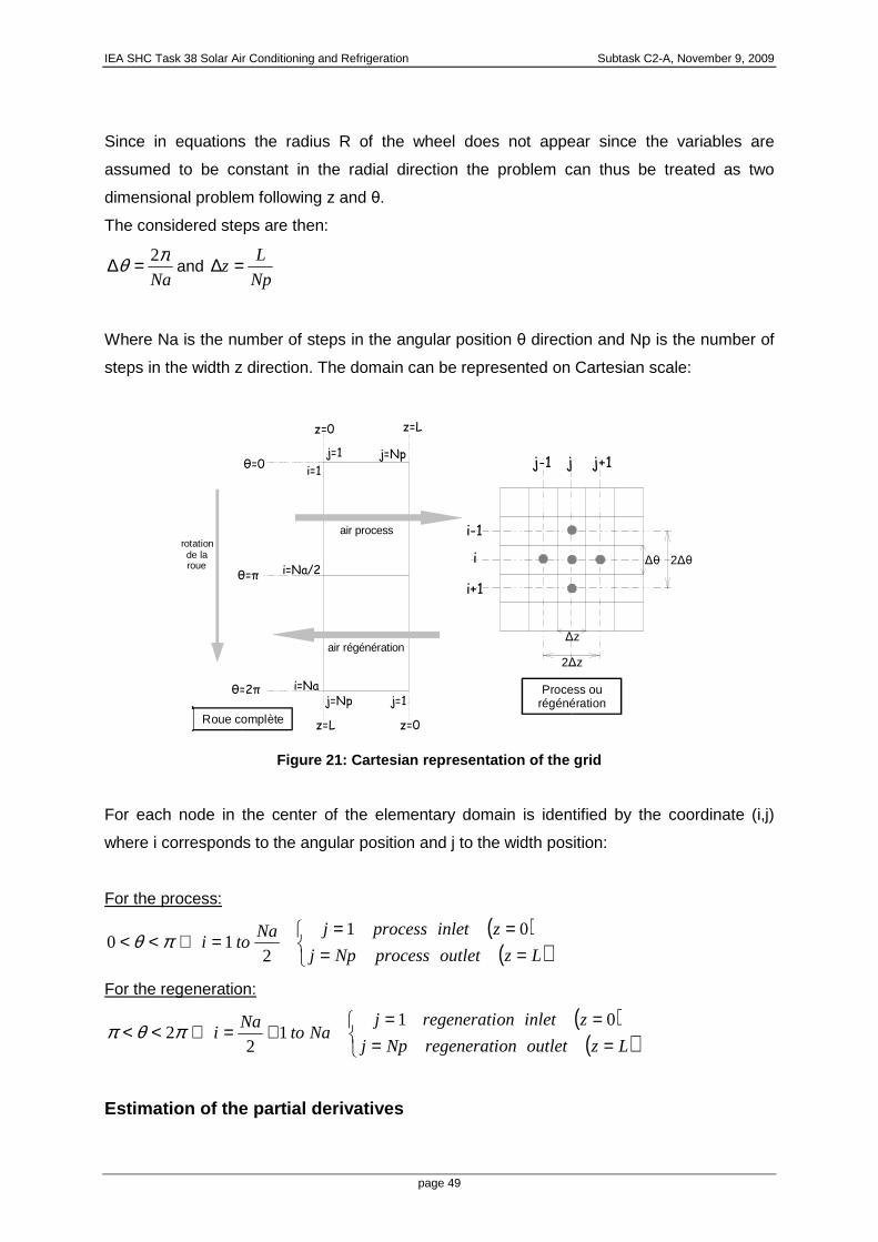
IEA SHC Task 38 Solar Air Conditioning and Refrigeration Subtask C2-A, November 9, 2009
page 49
Since in equations the radius R of the wheel does not appear since the variables are
assumed to be constant in the radial direction the problem can thus be treated as two
dimensional problem following z and θ.
The considered steps are then:
Na
πθ 2=∆ and Np
Lz =∆
Where Na is the number of steps in the angular position θ direction and Np is the number of
steps in the width z direction. The domain can be represented on Cartesian scale:
i
i-1
i+1
j j+1j-1
∆z
2∆z
∆θ 2∆θ
i=1
i=Na/2
i=Na
j=1 j=Np
z=0 z=L
θ=0
air process
air régénération
rotation de la roue
θ=π
θ=2π
z=0z=L
j=1j=Np
Roue complète
Process ou régénération
Figure 21: Cartesian representation of the grid
For each node in the center of the elementary domain is identified by the coordinate (i,j)
where i corresponds to the angular position and j to the width position:
For the process:
( )( )
====
=⇔<<LzoutletprocessNpj
zinletprocessjNatoi
01
210 πθ
For the regeneration:
( )( )
====
+=⇔<<LzoutletonregeneratiNpj
zinletonregeneratijNato
Nai
011
22πθπ
Estimation of the partial derivatives

IEA SHC Task 38 Solar Air Conditioning and Refrigeration Subtask C2-A, November 9, 2009
page 50
Figure 22: Current and neighbor nodes
The estimation of the partial derivatives is done using an upwind interpolation that permits
expressing the frontiers values in function of the considered node and in function of the
previous node.
The derivative with respect to θ:
( )θθ ∆
−=
∂∂ − jiji xxx ,1,
The derivative with respect to z:
( )z
xx
z
x jiji
∆−
=∂∂ −1,,
The moist air enthalpy is expressed by:
( )apvfgaapaa TchwTch .. ++= (35)
The desiccant enthalpy is expressed following Brandemuehl and Banks [18] and Stabat [11]
1−∆
++= −kWfgdpvdpd e
k
hTWcTcH
λ (36)
Replacing the enthalpies and derivative by the above equations, for each node (i,j) we have
finally:
Mass conservation equation
( ) ( ) ( ) 0*'' 1,,,1,,1, =−+−+− −−− jiajiaajiajiaajijid wwmwwmWWM (37)
Mass transfer equation
( ) jieqmjiamjijid wShwShWWM ,,,1, ''' −=−− − (38)
Heat conservation equation
x(i-1,j)
•
x(i,j)
•
x(j-1,j)
•
∆∆∆∆θ
∆∆∆∆z
D(i,j)

IEA SHC Task 38 Solar Air Conditioning and Refrigeration Subtask C2-A, November 9, 2009
page 51
( ) ( ) ( )( ) ( )
( ))exp()exp('
***
'
,1,
1,,1,1,,,
,1,,1,1,,,1,1,,
jijifgd
jiajiafgajiajiajiajia
jiajiafgajiajiajiajiajidjimjidjim
kWkWk
hM
wwhmTcTc
wwhmTcTcTcTc
−
−−−
−−−−−
−−−∆−=
−+−+
−+−+−
λ (39)
Heat transfer equation
( )( ) jieqjijifgd
jidcjiajijiajdijimjidjim
whkWkWk
hM
TShThwhTcTc
,,1,
,,,,,1,1,,
')exp()exp('
'*'
−−−−∆−=
+−−−
−
−−
λ (40)
With the following coefficients [19]
ro
dd
zMM
τπ ∆='
ro
aa
zmm
τπ ∆=' θ∆= umm aa *
zSS ∆∆= θ' fgm hShh ''=
( )jipvpddjim WccMc ,, ' += ( )jiapvpaajia wccmc ,, ' +=
( )jiapvpaajia wccmc ,, ** += ( ) ''* ,,, ShwwcShh cjieqjiapvmji +−=
For the details of the boundary conditions of the m odel please check the French
version of [1].
Model performance
The above presented model of the desiccant was implemented in SPARK. The figure below
shows the evolution of the air and the desiccant properties inside the wheel for an inlet
temperature of 30°C, inlet humidity ratio of 12 g/k g, regeneration temperature of 60°C and
regeneration humidity ratio of 12 g/kg. The figures show the temperature and the humidity
ratio distribution as a function of the angular position (0 to 180°) and as function of the width
(0 to 0.2m) of the wheel for the process sector.
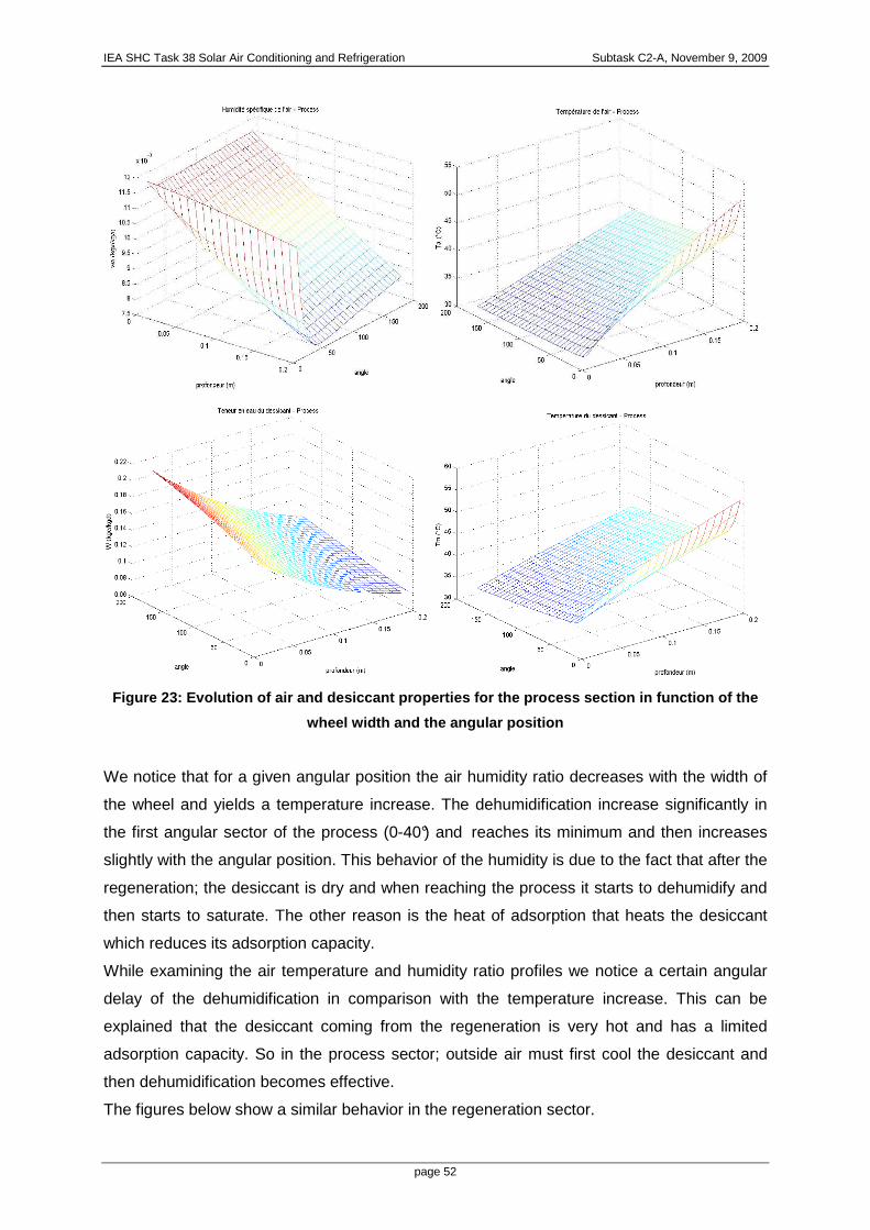
IEA SHC Task 38 Solar Air Conditioning and Refrigeration Subtask C2-A, November 9, 2009
page 52
Figure 23: Evolution of air and desiccant propertie s for the process section in function of the
wheel width and the angular position
We notice that for a given angular position the air humidity ratio decreases with the width of
the wheel and yields a temperature increase. The dehumidification increase significantly in
the first angular sector of the process (0-40°) and reaches its minimum and then increases
slightly with the angular position. This behavior of the humidity is due to the fact that after the
regeneration; the desiccant is dry and when reaching the process it starts to dehumidify and
then starts to saturate. The other reason is the heat of adsorption that heats the desiccant
which reduces its adsorption capacity.
While examining the air temperature and humidity ratio profiles we notice a certain angular
delay of the dehumidification in comparison with the temperature increase. This can be
explained that the desiccant coming from the regeneration is very hot and has a limited
adsorption capacity. So in the process sector; outside air must first cool the desiccant and
then dehumidification becomes effective.
The figures below show a similar behavior in the regeneration sector.
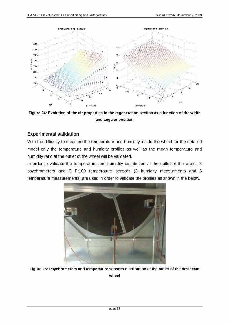
IEA SHC Task 38 Solar Air Conditioning and Refrigeration Subtask C2-A, November 9, 2009
page 53
Figure 24: Evolution of the air properties in the r egeneration section as a function of the width
and angular position
Experimental validation
With the difficulty to measure the temperature and humidity inside the wheel for the detailed
model only the temperature and humidity profiles as well as the mean temperature and
humidity ratio at the outlet of the wheel will be validated.
In order to validate the temperature and humidity distribution at the outlet of the wheel, 3
psychrometers and 3 Pt100 temperature sensors (3 humidity measurments and 6
temperature measurements) are used in order to validate the profiles as shown in the below.
Figure 25: Psychrometers and temperature sensors di stribution at the outlet of the desiccant
wheel
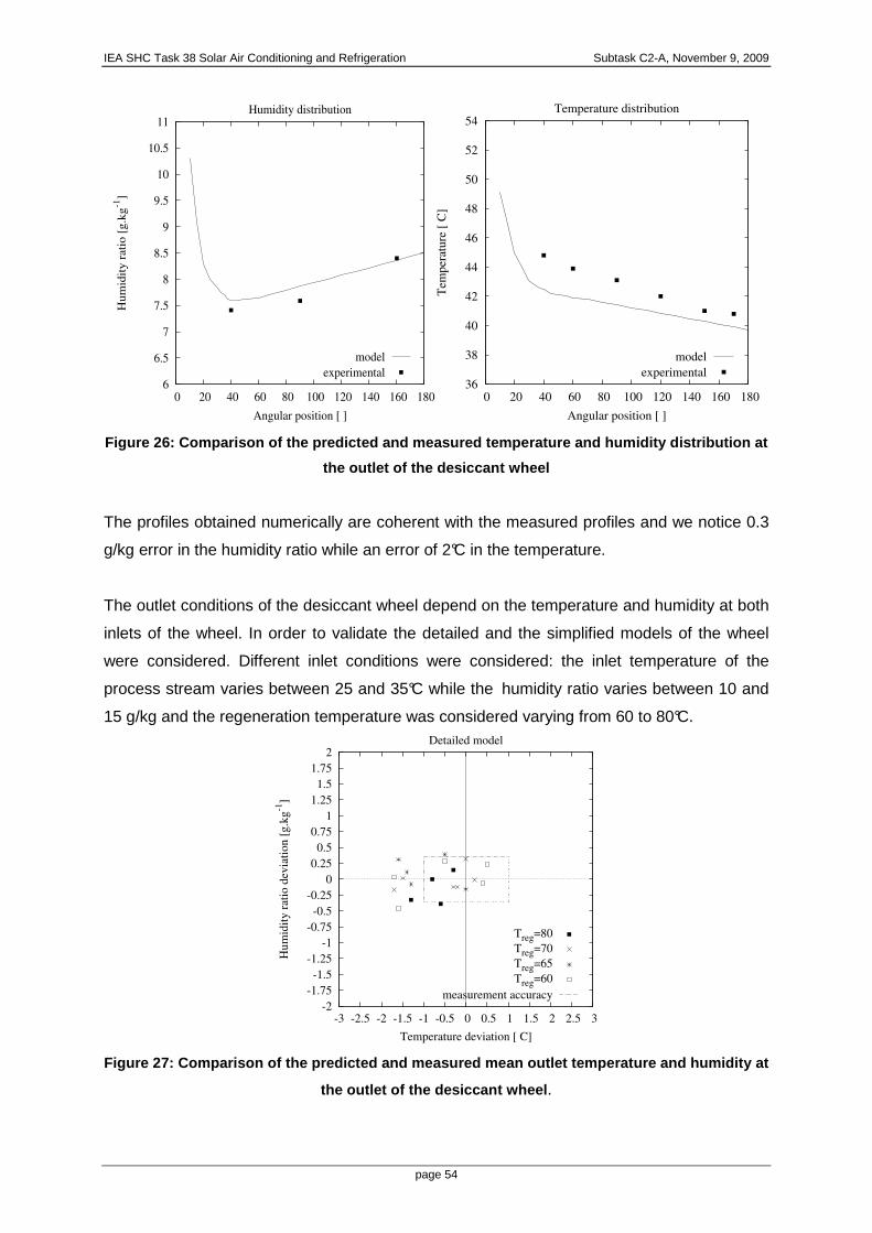
IEA SHC Task 38 Solar Air Conditioning and Refrigeration Subtask C2-A, November 9, 2009
page 54
6
6.5
7
7.5
8
8.5
9
9.5
10
10.5
11
0 20 40 60 80 100 120 140 160 180
Hum
idit
y r
ati
o [
g.k
g-1
]
Angular position [°]
Humidity distribution
model
experimental 36
38
40
42
44
46
48
50
52
54
0 20 40 60 80 100 120 140 160 180
Tem
per
ature
[°C
]
Angular position [°]
Temperature distribution
model
experimental
Figure 26: Comparison of the predicted and measured temperature and humidity distribution at
the outlet of the desiccant wheel
The profiles obtained numerically are coherent with the measured profiles and we notice 0.3
g/kg error in the humidity ratio while an error of 2°C in the temperature.
The outlet conditions of the desiccant wheel depend on the temperature and humidity at both
inlets of the wheel. In order to validate the detailed and the simplified models of the wheel
were considered. Different inlet conditions were considered: the inlet temperature of the
process stream varies between 25 and 35°C while the humidity ratio varies between 10 and
15 g/kg and the regeneration temperature was considered varying from 60 to 80°C.
-2
-1.75
-1.5
-1.25
-1
-0.75
-0.5
-0.25
0
0.25
0.5
0.75
1
1.25
1.5
1.75
2
-3 -2.5 -2 -1.5 -1 -0.5 0 0.5 1 1.5 2 2.5 3
Hum
idit
y r
atio
dev
iati
on [
g.k
g-1
]
Temperature deviation [°C]
Detailed model
Treg=80
Treg=70
Treg=65
Treg=60
measurement accuracy
Figure 27: Comparison of the predicted and measured mean outlet temperature and humidity at
the outlet of the desiccant wheel .

IEA SHC Task 38 Solar Air Conditioning and Refrigeration Subtask C2-A, November 9, 2009
page 55
Figure 27 gives the temperature and humidity ratio deviations at the outlet of the desiccant
wheel for the detailed. The maximum humidity ratio deviation of the detailed model is 0.4
g/kg and the maximum temperature deviation is 2°C. The uncertainty of the mean
temperature at the outlet of the wheel is in the order of 1 to 1.5°C (inhomogeneous outlet
with 10°C gradient) and the uncertainty of the humi dity ratio is 0.35 g/kg. The uncertainty of
the humidity is evaluated by comparing the mean humidity at the outlet of the wheel (position
2) with the absolute humidity at points 3, 4 and 5 (with reference to figure 1) while turning off
the supply humidifier. In these conditions the humidity must be constant. We notice that the
humidity ratio deviations are in the domain of the validity of the measurements. The detailed
model established of the physical description shows the same accuracy independently of the
regeneration temperature.
Conclusion
In this chapter a model of the solar desiccant installation is developed and validated
experimentally. First the components model considered solely showed acceptable accuracy
and low errors under different operating conditions. Then the overall model of the air
handling unit coupled with the solar installation gave satisfactory results for the considered
day and predicts accurately the supply air conditions. For the developed solar collector
model it showed a good accuracy in predicting the outlet temperature under transient
operating conditions and permits a good estimation of the potential of the collectors in
transient conditions. This model was used to elaborate control strategies and to optimize the
operations of the installation in function of outside and load conditions.
The developed detailed transient model of the desiccant wheel showed a good accuracy in
predicting the temperature and humidity distribution at the outlet of the wheel as well as the
mean outlet temperature and mean outlet humidity ratio. This detailed model is not suited for
seasonal simulation but it is very useful to elaborate control strategy and to study transient
behaviour of the desiccant air handling unit. The model can be used to study different
desiccant materials.

IEA SHC Task 38 Solar Air Conditioning and Refrigeration Subtask C2-A, November 9, 2009
page 56
References
[1]. Bourdoukan, P. "Etude numérique et expérimentale destinée à l’exploitation des
techniques de rafraîchissement par dessiccation avec régénération par énergie
solaire." Ph.D Thesis, Université La Rochelle, (2008) (Available in English)
[2]. Bourdoukan, P., Wurtz, E., Joubert, P., and Sperandio, M.. "Potential of solar heat
pipe vacuum collectors in the desiccant cooling process: modelling and experimental
results." Solar Energy 2008; 82(12): 1209-1219.
[3]. Bourdoukan, P., Wurtz, E., Joubert, P., and Spérandio, M. "Overall cooling
efficiency of a solar desiccant plant powered by direct flow vacuum tube collectors:
simulation and experimental results" Journal of Building Performance Simulation
2008, 1(3):149-162
[4]. Bourdoukan, P., Wurtz, E., Joubert, P.” Experimental investigation of a solar
desiccant cooling installation Solar Energy 83 (2009) 2059–2073
[5]. Bourdoukan, P., Wurtz, E., Joubert, P “omparison between the conventional and
recirculation modes in desiccant ooling cycles and deriving critical efficiencies of
components” Energy an International Journal, 2009 1-11 In press Corrected Proof.
doi:10.1016/j.energy.2009.06.021
[6]. Kays, W. M., and London, A. L. Compact Heat Exchangers, McGraw-Hill, New
York. (1984)
[7]. Maclaine-cross, I. L., and Banks, P. J. "Coupled heat and mass transfer in
regenerators- prediction using analogy with heat transfer." Int. J. Heat Mass Transfer
1972; 15: 1225-1242.
[8]. Banks, P. J. "Coupled equilibrium heat and single adsorbate transfer in field flow
through a porous medium- 1. Characteristics potentials and specific capacity ratios."
Chemical Engineering Science 1972; 27: 1143-1155.
[9]. Close, D. J., and Banks, P. J. "Coupled equilibrium heat and single adsorbate
transfer in field flow through a porous medium-2. Prediction for a silica gel air drier
using characteristic charts." Chemical Engineering Science 1972; 27: 1157-1168.
[10]. Jurinak, J. J. "Open cycle solid desiccant cooling - component models and system
simulation," Ph.D, University of Wisconsin, Madison. (1982)
[11]. Stabat, P. "Modélisation de composants de systèmes de climatisation mettant en
œuvre l'adsorption et l'évaporation d'eau," Ph.D Thesis, Ecole des Mines, Paris.
(2003)
[12]. Kamminga, W.. "The approximate temperature within a flate plate solar collector
under transient conditions." Int. J. Heat Mass Transfer, 28 (1985), 433-440.

IEA SHC Task 38 Solar Air Conditioning and Refrigeration Subtask C2-A, November 9, 2009
page 57
[13]. Schnieders, J.. "Comparison of the energy yield predictions of stationary and
dynamic solar collector models and the models' accuracy in the description of a
vacuum tube collector." Solar Energy, 61(1997), 179-190.
[14]. Klein, S. A.. "A Design Procedure for Solar Heating Systems," PhD, University of
Wisconsin-Madison (1976)
[15]. SPARK. "Simulation Problem Analysis and Research Kernel." LBNL, Berkeley,
California. (2003)
[16]. Sowell, E. F., and Taghavi, K. "Generation of building energy system models."
ASHRAE Transactions 1984, 106: 465-476.
[17]. Maclaine-cross, I. L. "A theory of combined heat and mass transfer in
regenerator," Ph.D, Univeristy of Monach, Australie. (1974).
[18]. Brandemuehl, M. J., and Banks, P. J.. "Rotary heat exchangers with time varying
or nonuniform inlet temperatures." ASME Journal of Heat Transfer, (1984) 106, 750-
758.
[19]. Le Garrec, S. "Modélisation des transferts de masse et de chaleur dans une roue
dessiccante," Master, ENTPE, Lyon. (2007).

IEA SHC Task 38 Solar Air Conditioning and Refrigeration Subtask C2-A, November 9, 2009
page 58

IEA SHC Task 38 Solar Air Conditioning and Refrigeration Subtask C2-A, November 9, 2009
page 59
Chapter III: New developments in simulation tools a nd models: A dynamic simulation model for transient absorption chiller performance. Paul Kohlenbach Solem Consulting Felix Ziegler Technische Universität Berlin, Institute for Energy Engineering This chapter presents the development of a dynamic model for single-effect LiBr/water
absorption chillers and its experimental validation.
In section (A) the developed model is presented in detail and compared to experimental data.
In section (B), general functionality of the model and a more detailed comparison with
experimental data are presented. This part also presents a more detailed investigation of the
model performance, including performance analysis, sensitivity checks. General model
functionality is demonstrated.
IEA SHC Task 38 Solar Air Conditioning and Refrigeration Subtask C2-A, November 9, 2009
page 60
1. A dynamic simulation model for transient absorption chiller performance. Part 1: the model
This section presents in detail the development of transient model for an absorption chiller.
The model is based on external and internal steady-state enthalpy balances for each main
component. Dynamic behaviour is implemented via mass storage terms in the absorber and
generator, thermal heat storage terms in all vessels and a delay time in the solution cycle.For
verification, the model has been compared to experimental data. The dynamic agreement
between experiment and simulation is very good with dynamic deviations around 10s.
Nomenclature
Symbols
A area, (m2)
A Duehring factor (deg C)
B Duehring factor (-)
c specific heat capacity (kJkg-1K-1)
c number of simulation steps representing time constants for transport delay (-)
D dew point temperature (deg C)
g gravity constant (Nm2kg-2)
h height difference between generator outlet and absorber inlet (m)
h enthalpy (kJkg-1)
l specific heat of solution (kJkg-1)
m, m& mass flow rate (kgs-1)
M mass (kg)
p pressure (Pa)
Q, Q& heat flux (kW)
r evaporation enthalpy (kJkg-1)
R gas constant for water vapour (Jkg-1)
T temperature (deg C)
t time (s)
UA heat transfer coefficient (kWK-1)
x Solution mass fraction (kgSaltkgSol-1)
X mole ratio (-)
z solution level in generator sump (m)
Greek letters
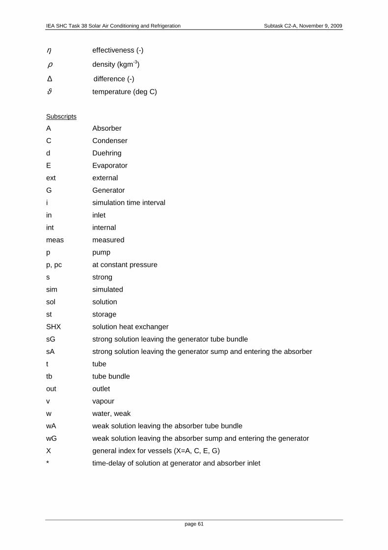
IEA SHC Task 38 Solar Air Conditioning and Refrigeration Subtask C2-A, November 9, 2009
page 61
η effectiveness (-)
ρ density (kgm-3)
∆ difference (-)
ϑ temperature (deg C)
Subscripts
A Absorber
C Condenser
d Duehring
E Evaporator
ext external
G Generator
i simulation time interval
in inlet
int internal
meas measured
p pump
p, pc at constant pressure
s strong
sim simulated
sol solution
st storage
SHX solution heat exchanger
sG strong solution leaving the generator tube bundle
sA strong solution leaving the generator sump and entering the absorber
t tube
tb tube bundle
out outlet
v vapour
w water, weak
wA weak solution leaving the absorber tube bundle
wG weak solution leaving the absorber sump and entering the generator
X general index for vessels (X=A, C, E, G)
* time-delay of solution at generator and absorber inlet

IEA SHC Task 38 Solar Air Conditioning and Refrigeration Subtask C2-A, November 9, 2009
page 62
Introduction
The dynamic model of an absorption chiller allows the simulation of its transient behaviour for
changing input conditions or design parameters. This is important because absorption
chillers usually have a high thermal mass, consisting of their internal heat exchangers, the
absorbing solution and the externally supplied heat transfer media. The dynamics of an
absorption chiller are therefore rather slow compared to similar capacity compression
chillers. The time to achieve a new steady-state with all parameters after a change of input
conditions is about 15 minutes for the chiller presented in this paper.
If the chiller is implemented in a complex heat supply/cooling demand system, e.g. a solar
thermal or waste-heat driven system, the simulation of the chiller is usually being done using
steady-state models. They simulate the chiller assuming constant operating conditions and
allow the determination of internal and external cycle parameters, such as heat exchanger
sizes, pump flow rates, temperatures and heat flows. However, steady-state models do not
provide time-dependent information on the thermal behaviour of absorption chillers and are
therefore not suitable for transient system simulations. In contrast, the model presented in
this work allows the simulation of the dynamic chiller behaviour. It extends the range of
applicable models for transient system simulations where the time constants of the chiller
significantly influence the system performance.
Research on dynamic system behaviour was carried out for both LiBr/water and water/NH3
heat pumps, chillers and components of such. Most complete are the recent papers by Bian
et al. [1], and Jeong et al. [2]. Bian et. al. [1] have performed a transient simulation of an
absorption chiller. They present a chiller model that can be run using variable time steps for
the simulation. It includes a temperature change term of each heat exchanger per time step
as well as a mass storage term in the generator, i.e. a part of the strong solution is being
stored in the generator in each time step. The model has been verified with experimental
data and shows good agreement in the transiency of the thermal behaviour, even if absolute
values do not exactly match.
Jeong et. al. [2] present the dynamic simulation of a steam-driven LiBr/water absorption heat
pump for the use of low-grade waste heat. The model assumes storage terms with thermal
capacities and solution mass storage in the vessels. Solution and vapour mass flow rates
are calculated in proportion to pressure differences between vessels. The heat transfer
coefficients as well as the simulation time step are assumed to be constant. The model has
been verified with good agreement using operational data for an absorption chiller.
The dynamic model presented here simulates the reaction of the absorption chiller on a
change of external conditions. In contrast to the approach in the cited references above, a
simpler model structure was chosen in order to learn more about the most important

IEA SHC Task 38 Solar Air Conditioning and Refrigeration Subtask C2-A, November 9, 2009
page 63
interdependencies in a direct manner. For instance, emphasis is on the fact that the thermal
storage terms respond partly to the temperatures of the external fluids and partly to the
internal process streams and these effects are separated. In contrast to this, the steady state
was incorporated very coarsely only, because time consuming iterations were to be avoided.
The model has been developed for and verified on the 10kW absorption chiller manufactured
by Phoenix SonnenWaerme AG [3].
Basic model Figure 1 shows the single-effect LiBr/water absorption cycle with state points as assumed for
the model.
Figure 1. LiBr/water absorption cycle.
Shown are the four main components of an absorption chiller: generator (G), condenser (C),
evaporator (E) and absorber (A). Also shown are solution heat exchanger, solution pump and
the throttling valves between absorber/solution heat exchanger and condenser/evaporator.
The internal state points characterize the thermodynamic properties of LiBr/water solution
(points 1-6), water vapour (7, 10) and liquid water (8, 9). The external state points
characterize the thermodynamic properties of hot water (11, 12), cooling water (13, 14, 15,
16) and chilled water (17, 18).
The input and output parameter of the model are given in the Appendix.

IEA SHC Task 38 Solar Air Conditioning and Refrigeration Subtask C2-A, November 9, 2009
page 64
From Figure 1 the steady-state internal heat flows of the vessels are as follows.
Evaporator: ( )810int, hhmQ vE −⋅= && (1)
Condenser: ( )87int, hhmQ vC −⋅= && (2)
Absorber: ( ) 5,1,10int, hmmhmhmQ vwsolwsolvA ⋅−+⋅−⋅= &&&&& (3)
Generator: ( ) 3,4,7int, hmhmmhmQ wsolvwsolvG ⋅−⋅−+⋅= &&&&& (4)
In equations (1) to (4), wsolm ,& is the mass flow of the diluted solution and vm& is the mass flow
of the refrigerant water vapour which is of equal value at state points 7 and 10 in Figure 1.
Equations (1) to (4) are based on the calculation of internal enthalpies for LiBr/water solution
and refrigerant vapour which requires sound knowledge of these properties. For
computational purposes this means that a property database of both LiBr/water and water
vapour has to be implemented into the simulation model and usually requires time-
consuming iterations.
The main aim of the model presented is to account for the dynamics. Therefore, no detailed
steady-state simulation with all state points was performed but a simpler approach was taken
which considers the most important physical properties only. This may be refined later on but
is not intended to be the focus of this work. This kind of refinement will not change the basic
findings of this report. So, to keep the model fast, equations (1) to (4) can be simplified using
the latent heat of evaporation and sorption, r and l, as shown in equations (6) to (9). This
approach has been proposed by Ziegler [4] to avoid a detailed enthalpy calculation for each
state point. Please note that the latent heat is taken at condenser pressure. The dependency
of latent heat on temperature is treated according to Plank’s rule [4].
Moreover, not all internal temperatures in Figure 1 are being calculated in the model.
Instead, each vessel is being modelled using external and internal mean temperatures of the
respective fluids (heat carrier and working fluid) as well as a mean vessel temperature.
External mean heat carrier temperatures Xϑ are being calculated using the arithmetic mean
temperature of inlet and outlet temperature. Internal mean temperatures XT are assumed to
be the mean of the equilibrium temperatures of strong and weak solution and of the

IEA SHC Task 38 Solar Air Conditioning and Refrigeration Subtask C2-A, November 9, 2009
page 65
condensing or evaporating refrigerant. Mean vessel temperatures XT are the arithmetic
mean temperature of the external and internal mean temperatures.
The boiling temperature of saturated LiBr/water solution can be calculated using the
Duehring relation, as described by Feuerecker [5]. In the model, this temperature is by
definition the mean of the equilibrium temperatures of strong (or weak) solution, xT .
DXBXAT ddx ⋅+= )()( (5)
with X being the mole fraction and D being the dew point temperature of the water vapour. Ad
and Bd are the Duehring coefficients which depend on the solution concentration but are
constant with regard to the dew point [5]. Some simplifying assumptions have been made for
the model. These are:
(a) There is no heat loss to or gain from the ambient.
(b) The pump work is neglected.
(c) The LiBr/water solution leaving generator and absorber tube bundle is saturated.
(d) The external inlet temperatures t11 , t13 , t17 are used as control parameters.
(e) The absorber cooling water outlet temperature equals the condenser inlet
temperature (t14=t15).
(f) The solution heat exchanger has a constant effectiveness SHXη .
(g) Water and LiBr/water solution have constant property data.
(h) The external and internal heat transfer coefficients (UA-values) are constant.
(i) Evaporation and solution enthalpy are constant.
(j) Constant pumping rate: The mass flow of weak solution from absorber to generator
is constant (state points 1, 2 and 3).
(k) The generator pressure equals the condenser pressure; the absorber pressure
equals the evaporator pressure.
Equations (1) to (4) do not account for dynamic effects. One way of accounting for a more
precise dynamic calculation is the introduction of different vapour mass flows for state points
7 and 10. The vapour mass flow from generator to condenser, Gvm ,& (state point 7), and from
evaporator to absorber, Avm ,& (state point 10), are therefore used in equations (6) to (9) which
describe the simplified internal enthalpy calculations.
( )( )ECvppcAvE TTcrmQ −⋅−⋅= ,)(,int, && (6)
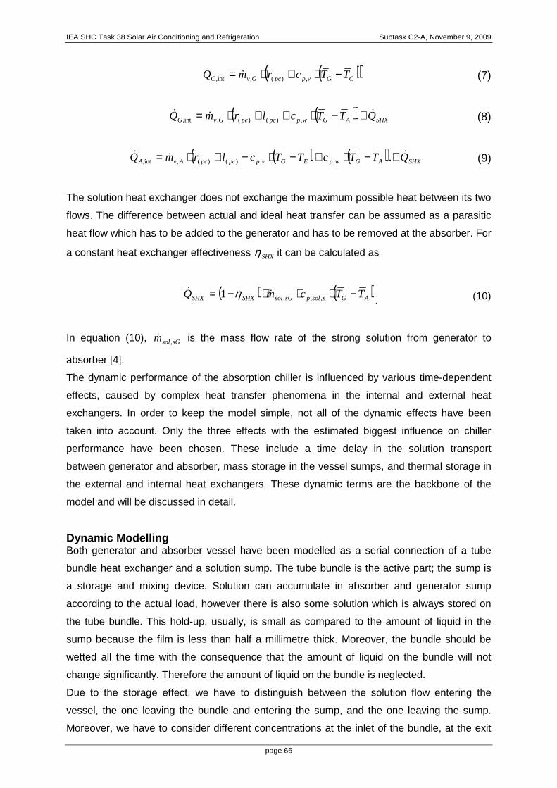
IEA SHC Task 38 Solar Air Conditioning and Refrigeration Subtask C2-A, November 9, 2009
page 66
( )( )CGvppcGvC TTcrmQ −⋅+⋅= ,)(,int, && (7)
( )( ) SHXAGwppcpcGvG QTTclrmQ &&& +−⋅++⋅= ,)()(,int, (8)
( ) ( )( ) SHXAGwpEGvppcpcAvA QTTcTTclrmQ &&& +−⋅+−⋅−+⋅= ,,)()(,int, (9)
The solution heat exchanger does not exchange the maximum possible heat between its two
flows. The difference between actual and ideal heat transfer can be assumed as a parasitic
heat flow which has to be added to the generator and has to be removed at the absorber. For
a constant heat exchanger effectiveness SHXη it can be calculated as
( ) ( )AGssolpsGsolSHXSHX TTcmQ −⋅⋅⋅−= ,,,1 && η. (10)
In equation (10), sGsolm ,& is the mass flow rate of the strong solution from generator to
absorber [4].
The dynamic performance of the absorption chiller is influenced by various time-dependent
effects, caused by complex heat transfer phenomena in the internal and external heat
exchangers. In order to keep the model simple, not all of the dynamic effects have been
taken into account. Only the three effects with the estimated biggest influence on chiller
performance have been chosen. These include a time delay in the solution transport
between generator and absorber, mass storage in the vessel sumps, and thermal storage in
the external and internal heat exchangers. These dynamic terms are the backbone of the
model and will be discussed in detail.
Dynamic Modelling Both generator and absorber vessel have been modelled as a serial connection of a tube
bundle heat exchanger and a solution sump. The tube bundle is the active part; the sump is
a storage and mixing device. Solution can accumulate in absorber and generator sump
according to the actual load, however there is also some solution which is always stored on
the tube bundle. This hold-up, usually, is small as compared to the amount of liquid in the
sump because the film is less than half a millimetre thick. Moreover, the bundle should be
wetted all the time with the consequence that the amount of liquid on the bundle will not
change significantly. Therefore the amount of liquid on the bundle is neglected.
Due to the storage effect, we have to distinguish between the solution flow entering the
vessel, the one leaving the bundle and entering the sump, and the one leaving the sump.
Moreover, we have to consider different concentrations at the inlet of the bundle, at the exit
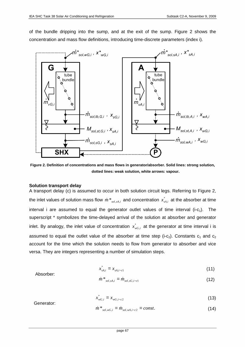
IEA SHC Task 38 Solar Air Conditioning and Refrigeration Subtask C2-A, November 9, 2009
page 67
of the bundle dripping into the sump, and at the exit of the sump. Figure 2 shows the
concentration and mass flow definitions, introducing time-discrete parameters (index i).
Figure 2. Definition of concentrations and mass flo ws in generator/absorber. Solid lines: strong soluti on,
dotted lines: weak solution, white arrows: vapour.
Solution transport delay A transport delay (c) is assumed to occur in both solution circuit legs. Referring to Figure 2,
the inlet values of solution mass flow isAsolm ,,*& and concentration ∗isAx , at the absorber at time
interval i are assumed to equal the generator outlet values of time interval (i-c1). The
superscript * symbolizes the time-delayed arrival of the solution at absorber and generator
inlet. By analogy, the inlet value of concentration ∗iwGx , at the generator at time interval i is
assumed to equal the outlet value of the absorber at time step (i-c2). Constants c1 and c2
account for the time which the solution needs to flow from generator to absorber and vice
versa. They are integers representing a number of simulation steps.
1,, cisAisA xx −∗ = (11)
Absorber: 1,,,,* cisGsolisAsol mm −= && (12)
2,, ciwGiwG xx −∗ = (13)
Generator: .* 2,,,, constmm ciwAsoliwGsol == −&& (14)

IEA SHC Task 38 Solar Air Conditioning and Refrigeration Subtask C2-A, November 9, 2009
page 68
As stated in equation (14) above, the mass flow of weak solution is set constant. In equation
(12) it is assumed that the mass flow entering the absorber tube bundle at time interval i
equals the mass flow which has left the generator c1 time intervals ago. Doing so, the
physical incompressibility of the solution in the piping between generator and absorber is not
modelled correctly. In reality, the mass flow entering the tube at time interval i should equal
the mass flow leaving the tube at time interval i. The assumption, however, had to be made
in order to achieve a correct salt balance in equation (22). The result is a hidden mass
storage term in the solution tube. However, the amount of stored solution in the tube is only
0.6 % of the total amount of stored solution in the sumps [3]. The error introduced by this
assumption is therefore negligible.
Mass balances The vessel sumps (see Figure 2) are assumed to be fully mixed at each time interval. Thus
vessel sump and solution leaving the vessel are assumed to have the same salt
concentration, xsA,i and xwG,i, respectively. The outlet of each tube bundle is assumed to
exhibit the equilibrium concentration xsG,i and xwA,i. The total solution mass stored in
generator and absorber sump at time i is expressed by iGstsolM ,,, and iAstsolM ,,, , respectively.
We know that the total mass (or salt mass, respectively) in the sump at time interval i equals
the total mass (or salt mass) at time interval (i-1) plus the difference of ingoing and outgoing
solution (or salt) flows at time interval i. The balances for the total solution contents in the
sumps are given in equations (15) and (16). t∆ is the time between two simulation intervals.
Generator: 01,,,,,,,,,,, =
∆−
−− −
t
MMmm iGstsoliGstsol
isGsoliGtbsol && (15)
Absorber: 01,,,,,,,,,,, =
∆−
−− −
t
MMmm iAstsoliAstsol
iwAsoliAtbsol && (16)
The fraction term in equations (15 and 16) is the amount of solution which is added to the
solution stored in either generator or absorber sump during the time t∆ between consecutive
simulation intervals i and (i-1).
The salt flow balance, analogously, in both sumps can be written as:
Generator
: 01,1,,,,,,,
,,,,,,, =∆
⋅−⋅−⋅−⋅ −−
t
xMxMxmxm isAiGstsolisAiGstsol
isAisGsolisGiGtbsol &&
(17
)
Absorber
: 01,1,,,,,,,
,,,,,,, =∆
⋅−⋅−⋅−⋅ −−
t
xMxMxmxm iwGiAstsoliwGiAstsol
iwGiwAsoliwAiAtbsol &&
(18
)

IEA SHC Task 38 Solar Air Conditioning and Refrigeration Subtask C2-A, November 9, 2009
page 69
Proceeding from the sumps to the tube bundles, the mass flow balance yields
Generator: 0,,,,2,, =−−− iGtbsolivGciwAsol mmm &&& (19)
Absorber: 0,,,,1,, =−+− iAtbsolivAcisGsol mmm &&& (20)
The salt flow balances of the tube bundles read
Generator: 0,,,,2,2,, =⋅−⋅ −− isGiGtbsolciwGciwAsol xmxm && (21)
Absorber: 0,,,,1,1,, =⋅−⋅ −− iwAiAtbsolcisAcisGsol xmxm && (22)
Pressure drop The strong solution flow from generator to absorber is driven by gravity and a pressure
difference. The pressure loss of the solution heat exchanger and its adjacent piping is
assumed constant which is a good approximation as long as the flow variations are not too
large; hence the mass flow of the strong solution depends only on the pressure difference
between generator/absorber and the liquid solution column at heat exchanger inlet. This
assumption, of course, can be refined in future works. During operation, the static pressure
of the liquid column has to equal the dynamic pressure loss caused by flow restrictions
through piping and solution heat exchanger. The mass flow of the strong solution can
therefore be calculated as
( )( )
ςρρ issoliAiGssol
tissol
zhgppAm
+⋅⋅+−⋅⋅⋅= ,,,,
,,
2& , (23)
where generator/condenser and evaporator/absorber pressure are calculated using the
equation of Clausius-Clapeyron as shown in equation (24). There, the pressure and
temperature values of solution interval (i-1) are being used to calculate the values of
simulation interval i. This is a valid approximation as long as the time between two simulation
intervals, t∆ , is not too long.
−⋅=
−− iXiXiX
iX
TTR
r
p
p
,1,
0
1,
, 11ln (24)
Thermal storage
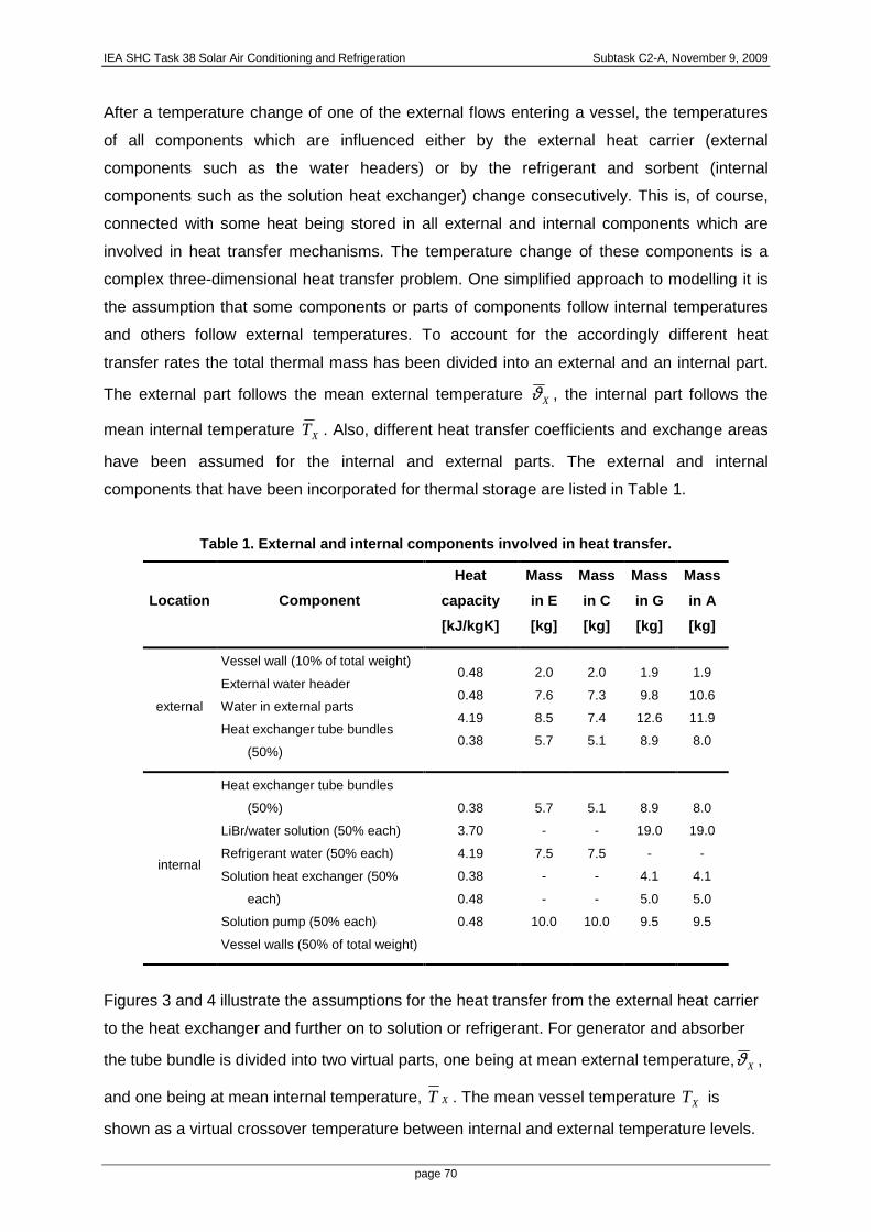
IEA SHC Task 38 Solar Air Conditioning and Refrigeration Subtask C2-A, November 9, 2009
page 70
After a temperature change of one of the external flows entering a vessel, the temperatures
of all components which are influenced either by the external heat carrier (external
components such as the water headers) or by the refrigerant and sorbent (internal
components such as the solution heat exchanger) change consecutively. This is, of course,
connected with some heat being stored in all external and internal components which are
involved in heat transfer mechanisms. The temperature change of these components is a
complex three-dimensional heat transfer problem. One simplified approach to modelling it is
the assumption that some components or parts of components follow internal temperatures
and others follow external temperatures. To account for the accordingly different heat
transfer rates the total thermal mass has been divided into an external and an internal part.
The external part follows the mean external temperature Xϑ , the internal part follows the
mean internal temperature XT . Also, different heat transfer coefficients and exchange areas
have been assumed for the internal and external parts. The external and internal
components that have been incorporated for thermal storage are listed in Table 1.
Table 1. External and internal components involved in heat transfer.
Location Component
Heat
capacity
[kJ/kgK]
Mass
in E
[kg]
Mass
in C
[kg]
Mass
in G
[kg]
Mass
in A
[kg]
external
Vessel wall (10% of total weight)
External water header
Water in external parts
Heat exchanger tube bundles
(50%)
0.48
0.48
4.19
0.38
2.0
7.6
8.5
5.7
2.0
7.3
7.4
5.1
1.9
9.8
12.6
8.9
1.9
10.6
11.9
8.0
internal
Heat exchanger tube bundles
(50%)
LiBr/water solution (50% each)
Refrigerant water (50% each)
Solution heat exchanger (50%
each)
Solution pump (50% each)
Vessel walls (50% of total weight)
0.38
3.70
4.19
0.38
0.48
0.48
5.7
-
7.5
-
-
10.0
5.1
-
7.5
-
-
10.0
8.9
19.0
-
4.1
5.0
9.5
8.0
19.0
-
4.1
5.0
9.5
Figures 3 and 4 illustrate the assumptions for the heat transfer from the external heat carrier
to the heat exchanger and further on to solution or refrigerant. For generator and absorber
the tube bundle is divided into two virtual parts, one being at mean external temperature, Xϑ ,
and one being at mean internal temperature, XT . The mean vessel temperature XT is
shown as a virtual crossover temperature between internal and external temperature levels.

IEA SHC Task 38 Solar Air Conditioning and Refrigeration Subtask C2-A, November 9, 2009
page 71
Figure 3 shows the partition of the generator vessel into the external (right side) and internal
(left side) part, Figure 4 shows the same partition for the absorber.
Figure 3. Enthalpy balance for generator vessel. Gre y arrows: heat flow, white arrow: vapour flow, blac k
arrows: fluid flow. Left side: internal, right side : external
Figure 4. Enthalpy balance for absorber vessel. Grey arrows: heat flow, white arrow: vapour flow, black
arrows: fluid flow. Left side: internal, right side : external
Externally, all four chiller vessels incorporate water headers for the distribution of hot, chilled
and cooling water through the tube bundles. It is assumed that the headers and the water
mass enclosed in those contribute completely to the external heat storage. The tube bundles
are assumed to contribute by 50% of their mass to the external heat storage and by 50% to
the internal heat storage. This is reasonable because the falling film heat exchanger tubes
have flow on both sides, internally by LiBr/water solution and externally by water. The vessel
wall is assumed to contribute by 10% of its total weight to the external thermal mass due to
the conduction heat transfer from the headers.

IEA SHC Task 38 Solar Air Conditioning and Refrigeration Subtask C2-A, November 9, 2009
page 72
Internally, in addition to the tube bundles, the solution contributes by 50% of its mass in
generator and absorber. In analogy, the refrigerant is assumed to have a 50% internal
contribution in both evaporator and condenser. The mass of solution heat exchanger and
solution pump has an internal effect on both generator and absorber heat transfer and is
assumed to contribute by 50% of its weight on both. The vessel wall now contributes
internally by 50% of its weight due to the larger surface area involved in heat transfer mainly
in the sumps.
Enthalpy balances Taking internal and external thermal storage as in Figures 3 and 4 into account, equations
(6) to (9) can be refined and the external and internal enthalpy balances for the vessels can
now be expressed. The external enthalpy balance of the vessels describes that the heat
which is given off (generator) or taken on (absorber) by the heat carrier (left-hand side of
equation (25) or (26)) partly crosses the heat exchanger (first term on the right-hand side,
grey arrows in Figures 3 and 4) and reaches the mean vessel temperature, partly is used to
heat up parts of the vessel which are more or less at external temperature (second term on
right-hand side). For generator and evaporator, the external enthalpy balance reads
( ) ( ) ( ) ( )t
cMTUAcm iXiX
XextpiXiXXextoutXinXwpwX ∆−
⋅⋅+−⋅=−⋅⋅ −1,,
,,,,,,,,
ϑϑϑϑϑ& (25)
In equation (25), index X denotes the different vessels of generator and evaporator (X = G,
E). For absorber and condenser the external enthalpy balance reads
( ) ( ) ( ) ( )t
cMTUAcm iXiX
XextpiXiXXextoutXinXwpwX ∆−
⋅⋅−−⋅−=−⋅⋅ −1,,
,,,,,,,,
ϑϑϑϑϑ& (26)
Index X in equation (26) denotes absorber and condenser (X = A, C).
The internal enthalpy balances for all vessels read as follows.
( )( ) ( ) ( )iEiEE
iEiE
EpiEiCvppciAv TTUAt
TTcMTTcrm ,,int,
1,,
int,,,,)(,, )( −⋅=
∆−⋅⋅+−⋅−⋅ −
& (27)
( )( ) ( )( ) ( )iGiGG
iGiG
GpiSHXiAiGiwppcpciGv
TTUA
t
TTcMQTTclrm
,,int,
1,,
int,,,,,,)()(,,
−⋅=∆−⋅⋅++−⋅++⋅ −&&
(28)

IEA SHC Task 38 Solar Air Conditioning and Refrigeration Subtask C2-A, November 9, 2009
page 73
( )( ) ( ) ( ) ( )iCiCC
iCiC
CpiCiGvppciGv TTUAt
TTcMTTcrm ,,int,
1,,
int,,,,)(,, −⋅=
∆−⋅⋅+−⋅+⋅ −
& (29)
( ) ( )( )( ) ( ) ( )iAiAA
iAiA
Ap
iSHXiAiGwpiEiGvppcpciAv
TTUAt
TTcM
QTTcTTclrm
,,int,
1,,
int,
,,,,,,,)()(,,
−⋅=∆−⋅⋅
++−⋅+−⋅−+⋅
−
&&
(30)
Equations (27) and (28) describe the internal heat transfer in evaporator and generator,
respectively. There, the heat which is given off by the heat exchanger (right-hand side) partly
heats up the internal parts of the vessel (second term on left-hand side) and partly is used for
the heating of solution and refrigerant (first term on left-hand side). In analogy, equations (29)
and (30) describe condenser and absorber, respectively. There, the heat which is given off
by the solution and refrigerant (first term on left-hand side) is used partly to heat the internal
parts of the heat exchanger (second term on left-hand side) and partly to heat the cooling
water (right-hand side).
The equation system is being solved in MATLAB using a Newton-Raphson procedure with
finite-difference Jacobian approximation [6].
Experimental Verification The agreement between simulated and experimental data has been tested using an
experimentally measured hot water input step from 75 to 85 °C. The results of the simulation
using these input data are shown in Figure 5. The hot water inlet and outlet temperatures in
Figure 5 are taken from experimental measurements of the Phoenix absorption chiller. They
show the transient behaviour of the chiller for a 10K step in hot water inlet temperature.
Cooling and chilled water inlet temperatures as well as all external mass flow rates were kept
constant during the step. It can be seen that it takes approx. 600s or 10 minutes to achieve a
new steady-state in hot water inlet temperature after the step. This is shorter than the 15
minutes it takes for all parameters to achieve steady-state again. The simulation was
performed using the measured data as inputs in the model and comparing simulated and
measured hot water outlet temperatures.

IEA SHC Task 38 Solar Air Conditioning and Refrigeration Subtask C2-A, November 9, 2009
page 74
Figure 5. Comparison of simulated and measured gene rator outlet temperatures.
Figure 5 shows that the steady-state agreement between measured and simulated values is
reasonably well despite the fact that steady-state accuracy has been incorporated coarsely
only. At simulation start, the simulated temperatures diverge slightly from the initial measured
state towards a different steady-state. In general, the temperature difference between
experiment and simulation is larger after the step which shows that there is a dependency of
the model output on the hot water temperature. This can be related to temperature-
dependent parameters which have been assumed constant for the simulation, such as
evaporation and solution enthalpy, density and specific heat capacity. As steady-state
accuracy is not the focus in this paper this deviation shall not be discussed further.
Much more important is the fact that the dynamic agreement between measured and
simulated output data is very good. Figure 5 shows that the fluctuations of simulated and
measured hot water outlet temperature are well synchronized, although there is a slight delay
of approximately 10 seconds of measured to simulated values. This has to be put into
relation to the 600 seconds or 10 minutes that it takes to reach a steady state in the
generator temperatures again.
The delay between simulation and experiment can – at least to some extent - be explained
with the assumptions of thermal mass for the individual vessels in Table 1 which have not
been verified yet. Another reason for the disagreement is the fact that some time delays

IEA SHC Task 38 Solar Air Conditioning and Refrigeration Subtask C2-A, November 9, 2009
page 75
existing in reality have not been incorporated into the model. These include the forced
circulation of refrigerant in the evaporator by means of a second internal pump. Also, the
condensed refrigerant flowing from condenser to evaporator has a time delay which has
been neglected. There is no vapour storage in the vessels assumed. The transport delay c1
has been assumed constant although it changes in proportion to the strong solution mass
flow. The transport delay in the cooling water between absorber outlet and condenser inlet
due to piping length has also been neglected as well as the change in solution storage on the
tube bundles. These time delays have not been included in order to keep the model as
simple as possible.
The results in Figure 5 are shown here just in order to demonstrate the basic functionality of
the model. A sensitivity analysis along with more experimental data is presented in the
second part of this paper [7].
Conclusions
In this paper a dynamic model for absorption chillers has been presented. It is based on
internal energy balances as well as mass balances. Dynamic behaviour is implemented via
eight thermal and two mass storage terms as well as by two delay times. The heat transfer
has been divided into two parts: one which transfers heat from the external heat carrier to the
exchanger material and the second from there on to the refrigerant or solution side, or vice
versa. In this way the thermal mass of the vessel could be introduced easily. The agreement
between experiment and simulation is very good with deviations of 10s for the generator. The
total time to achieve a new steady-state after an input temperature step amounts to
approximately 15 minutes. Compared to this, the present dynamic deviations are in the
magnitude of approximately 1%.
More information about the simulation results, comparison with experiments and sensitivity
checks will be presented in the second part of this paper [7].

IEA SHC Task 38 Solar Air Conditioning and Refrigeration Subtask C2-A, November 9, 2009
page 76
Appendix
Inputs and outputs of the dynamic model
Table 2. Input parameter of the dynamic model.
No. Inputs Unit Description 1 ϑ 11,i °C Generator hot water inlet temperature at time 2 ϑ 17,i °C Evaporator chilled water inlet temperature at 3 ϑ 13,i °C Absorber cooling water inlet temperature at time 4 ϑ 18,i-1 °C Evaporator chilled water outlet temperature at 5 ϑ 16,i-1 °C Condenser cooling water outlet temperature at 6 ϑ 12,i-1 °C Generator hot water outlet temperature at time 7 ϑ 14,i-1 °C Absorber cooling water outlet temperature at 8 1, −iET °C Internal mean temperature of evaporator at time 9 1, −iCT °C Internal mean temperature of condenser at time
10 1, −iGT °C Internal mean temperature of generator at time 11 1, −iAT °C Internal mean temperature of absorber at time 12
2,,, ciGwsolx − kgSaltkgSol- Solution concentration of absorber sump at time
13 1,,, ciAssolx − kgSaltkgSol
- Solution concentration of generator sump at time 14
1,, cissolm −& kgs-1 Strong solution mass flow at time interval i-c1 15
1,, −iGsx kgSaltkgSol- Equilibrium concentration in generator at time
16 1,, −iAsx kgSaltkgSol
- Solution concentration of generator sump at time 17
1,, −iGwx kgSaltkgSol- Solution concentration of absorber sump at time
18 1,, −iAwx kgSaltkgSol
- Equilibrium concentration in absorber at time
19 1,,, −iGsolstM kg Total mass in generator sump at time interval i-1
20 1,,, −iAsolstM kg Total mass in absorber sump at time interval i-1
21 t∆ s Time period between time intervals i and i-1

IEA SHC Task 38 Solar Air Conditioning and Refrigeration Subtask C2-A, November 9, 2009
page 77
Table 3. Output parameter of the dynamic model.
No. Outputs Unit Description 1 ϑ 18,i °C Evaporator chilled water outlet temperature at t ime 2 ϑ 16,i °C Condenser cooling water outlet temperature at ti me 3 ϑ 12,i °C Generator hot water outlet temperature at time 4 ϑ 14,i °C Absorber cooling water outlet temperature at tim e 5 iET , °C Internal mean temperature of evaporator at time 6 iCT , °C Internal mean temperature of condenser at time 7 iGT , °C Internal mean temperature of generator at time 8 iAT , °C Internal mean temperature of absorber at time 9
iGvm ,,& kgs-1 Vapour mass flow from generator to condenser at 10
iAvm ,,& kgs-1 Vapour mass flow from evaporator to absorber at 11
iGsx ,, kgSaltkgSol- Equilibrium concentration in generator at time
12 iAsx ,, kgSaltkgSol
- Solution concentration of generator sump at time 13
iAwx ,, kgSaltkgSol- Equilibrium concentration in absorber at time interval
14 iGwx ,, kgSaltkgSol
- Solution concentration of absorber sump at time 15
iGtbsolm ,,,& kgs-1 Solution mass flow after tube bundle in generator 16
iAtbsolm ,,,& kgs-1 Solution mass flow after tube bundle in absorber 17
iGsolstm ,,, kg Stored solution in generator sump at time interval i 18
iAsolstm ,,, kg Stored solution in absorber sump at time interval i 19 zi m Height of solution level in generator sump at time 20
issolm ,,& kgs-1 Strong solution mass flow at time interval i 21
iGp , Pa Generator/condenser pressure at time interval i 22
iAp , Pa Evaporator/absorber pressure at time interval i
23 iGsolstM ,,, kg Total solution mass in generator at time interval i
24 iAsolstM ,,, kg Total solution mass in absorber at time interval i
IEA SHC Task 38 Solar Air Conditioning and Refrigeration Subtask C2-A, November 9, 2009
page 78
References
[1] Bian J, Radermacher R, Moran D. Transient simulation of an absorption chiller in a
CHP system. In Proceedings of the International Sorption Heat Pump Conference,
June 22-24, 2005, Denver, CO, USA.
[2] Jeong S, Kang BH, Karng SW. Dynamic simulation of an absorption heat pump for
recovering low grade waste heat. Applied Thermal Engineering 1998; 18 (1-2); 1-12
[3] Kohlenbach P. Solar cooling systems with absorption chillers: Control strategies and
transient chiller performance. 2006; PhD Thesis; Technical University of Berlin,
Forschungsberichte des Deutschen Kälte- und Klimatechnischen Vereins; Nr. 74,
Erding, Germany
[4] Ziegler F. Sorptionswärmepumpen. 1997; Habilitation Thesis; Forschungsberichte
des Deutschen Kälte- und Klimatechnischen Vereins; Nr. 57, Erding, Germany.
[5] Feuerecker G. Entropieanalyse für Wärmepumpensysteme: Methoden und
Stoffdaten. 1994; PhD thesis; Faculty of Physics; Technical University of Munich;
Germany.
[6] Urroz GE. Solution of non-linear equations. 2004; Lecture handout; Utah State
University; U.S.A.
[7] Kohlenbach P, Ziegler F. A dynamic simulation model for transient absorption chiller
performance. Part II: Numerical results and experimental verification. 2007; Int J
Refrigeration, this issue.

IEA SHC Task 38 Solar Air Conditioning and Refrigeration Subtask C2-A, November 9, 2009
page 79
2. A dynamic simulation model for transient absorption chiller performance: Numerical results and experimental verification
This section describes the performance and experimental verification of a dynamic absorption chiller model. In [1] the model itself was described with regard to dynamic effects, such as transport delays in the solution circuit, thermal storage and mass storage. In detail, the size of the solution sumps in absorber and generator, the time for the solution to flow from absorber to generator and vice-versa and the thermal mass of the main components has been accounted for. As a special feature, the thermal mass of the components has been split into two parts, one which responds to the temperature of the external fluids, and the other which responds to the temperature of the solution and the refrigerant (internal fluids). These are the main parameters which determine the dynamic behaviour of the chiller. This second section is looking at internal consistency, sensitivity and accuracy of the model. Results of a performance analysis using ideal conditions to prove correct model behaviour are shown. A sensitivity analysis on thermal storage and solution transport delay has been performed to investigate the influence of the dynamic parameters on the chiller performance. Finally, a model verification using experimental results is also given in this paper.
Nomenclature
Symbols
A area, (m2) A Duehring factor (deg C) B Duehring factor (-) c specific heat capacity (kJkg-1K-1) c number of simulation steps representing time constants for transport delay (-) D dew point temperature (deg C) g gravity constant (Nm2kg-2) h height difference between generator outlet and absorber inlet (m) h enthalpy (kJkg-1) l specific heat of solution (kJkg-1)
m, m& mass flow rate (kgs-1)
M mass (kg) p pressure (Pa)
Q& ,Q heat flux (kW)
r evaporation enthalpy (kJkg-1) R gas constant for water vapour (Jkg-1) T temperature (deg C) t time (s) UA heat transfer coefficient (kWK-1) x Solution mass fraction (kgSaltkgSol
-1) X mole ratio (-) z solution level in generator sump (m)
IEA SHC Task 38 Solar Air Conditioning and Refrigeration Subtask C2-A, November 9, 2009
page 80
Greek letters
η effectiveness (-)
ρ density (kgm-3)
∆ difference (-)
ϑ temperature (deg C)
Subscripts
A Absorber Acc Cooling water inlet Ach Cooling water outlet C Condenser d Duehring E Evaporator Eh Chilled water inlet Ec Chilled water outlet ext external G Generator Gc Hot water outlet i simulation time interval in inlet int internal meas measured p pump p, pc at constant pressure s strong sim simulated sol solution st storage SHX solution heat exchanger sG strong solution leaving the generator tube bundle sA strong solution leaving the generator sump and entering the absorber t tube tb tube bundle out outlet v vapour w water, weak wA weak solution leaving the absorber tube bundle wG weak solution leaving the absorber sump and entering the generator X general index for vessels (X=A, C, E, G) Performance analysis The internal consistency of the model can be analysed by applying a step change to one of the external parameters in the model. A step from 75°C to 85°C in the hot water inlet temperature has been used for this purpose. Cooling and chilled water inlet temperatures

IEA SHC Task 38 Solar Air Conditioning and Refrigeration Subtask C2-A, November 9, 2009
page 81
have been kept constant at 27°C and 18°C, respectiv ely. The simulation interval was 1s. The temperature step was set at 200s after simulation start. This time period is necessary because the preset steady-state is not exactly met by the model: after starting the simulation first the steady state with the given input values has to be reached. 200s are enough in order to equalize the differences between initial and steady-state values. For the consistency analysis no thermal storage terms were assumed, just solution mass storage and a transport delay of 2 steps or seconds between generator and absorber and 1 step or second the other way. These very short transport delays were chosen to speed up the simulation. Figure 1 shows some internal variables for a short time period before and after the temperature step. Figure 2 shows the external heat flows before and after the temperature step. Each marker symbol in the graph denotes one simulation step.

IEA SHC Task 38 Solar Air Conditioning and Refrigeration Subtask C2-A, November 9, 2009
page 82
Figure 1. Simulated chiller response on 10K step in generator inlet temperature without thermal mass.

IEA SHC Task 38 Solar Air Conditioning and Refrigeration Subtask C2-A, November 9, 2009
page 83
Figure 2. External heat flows of simulated chiller r esponse on 10K step in generator inlet temperature
without thermal mass
In Figure 1, graph 1 shows the temperatures in the generator which follow immediately the step of the external inlet temperature, t11, because no thermal storage has been assumed. Accordingly, the heat flow to the generator increases (Figure 2, top left graph). The strong solution leaving the generator bundle follows immediately (xsG in graph 4 of Figure 1). The strong solution leaving the generator sump follows in a damped fashion (xsA in graph 4) because of the mass storage in the sump. The first change in mass fraction of the strong solution reaches the absorber inlet two steps later. Three steps after the initial change the mass fraction of the weak solution leaving the absorber bundle begins to change as well (xwA in graph 4); the solution in the sump follows as well (xwG in graph 4) but this is hardly visible due to the damping effect of the mass which is stored in the sump. The flow of weak solution is kept constant (msol,w in graph 7). The flow of strong solution increases immediately (msol,s in graph 7). This due to the rise in generator pressure (pG in graph 5), which drives more solution through the expansion valve. The rise in pressure, in turn is a consequence of the rise in the condenser heat flow (Figure 2, top right graph) due to the rise of vapour mass flow to the condenser (mvG in graph 6). The flow of strong solution from the generator bundle to the generator sump (mtbG in graph 8) decreases because the inlet flow is constant and more vapour is being produced. Of course, also the mean generator and condenser temperature (TG in graph 1 and TC in graph 2), and the condenser cooling water outlet temperature (t16 in graph 2) increases. When the more concentrated solution reaches the absorber in step 204, the pressure immediately falls (pA in graph 5). The absorber absorbs more vapour, the vapour flow from evaporator to absorber increases (mvA in graph 6 of Figure 1), the flow from the absorber bundle to the sump increases (mtbA in graph 8), and the absorber heat increases (Figure 2, bottom right graph). Accordingly, the temperature of the cooling water leaving the absorber increases (t14 in graph 2). At the same time, the evaporator heat increases (Figure 2, bottom
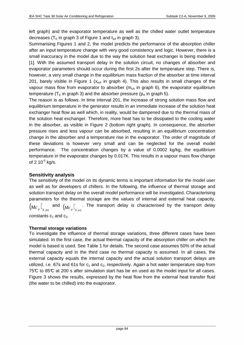
IEA SHC Task 38 Solar Air Conditioning and Refrigeration Subtask C2-A, November 9, 2009
page 84
left graph) and the evaporator temperature as well as the chilled water outlet temperature decreases (TE in graph 3 of Figure 1 and t18 in graph 3). Summarising Figures 1 and 2, the model predicts the performance of the absorption chiller after an input temperature change with very good consistency and logic. However, there is a small inaccuracy in the model due to the way the solution heat exchanger is being modelled [1]. With the assumed transport delay in the solution circuit, no changes of absorber and evaporator parameters should occur during the first 2s after the temperature step. There is, however, a very small change in the equilibrium mass fraction of the absorber at time interval 201, barely visible in Figure 1 (xwA in graph 4). This also results in small changes of the vapour mass flow from evaporator to absorber (mvA in graph 6), the evaporator equilibrium temperature (TE in graph 3) and the absorber pressure (pA in graph 5). The reason is as follows. In time interval 201, the increase of strong solution mass flow and equilibrium temperature in the generator results in an immediate increase of the solution heat exchanger heat flow as well which, in reality, would be dampened due to the thermal mass of the solution heat exchanger. Therefore, more heat has to be dissipated to the cooling water in the absorber, as visible in Figure 2 (bottom right graph). In consequence, the absorber pressure rises and less vapour can be absorbed, resulting in an equilibrium concentration change in the absorber and a temperature rise in the evaporator. The order of magnitude of these deviations is however very small and can be neglected for the overall model performance. The concentration changes by a value of 0.0002 kg/kg, the equilibrium temperature in the evaporator changes by 0.017K. This results in a vapour mass flow change of 2 10-5 kg/s.
Sensitivity analysis The sensitivity of the model on its dynamic terms is important information for the model user as well as for developers of chillers. In the following, the influence of thermal storage and solution transport delay on the overall model performance will be investigated. Characterising parameters for the thermal storage are the values of internal and external heat capacity,
( )int,XpMc and ( )
extXpMc,
. The transport delay is characterised by the transport delay
constants c1 and c2. Thermal storage variations To investigate the influence of thermal storage variations, three different cases have been simulated. In the first case, the actual thermal capacity of the absorption chiller on which the model is based is used. See Table 1 for details. The second case assumes 50% of the actual thermal capacity and in the third case no thermal capacity is assumed. In all cases, the external capacity equals the internal capacity and the actual solution transport delays are utilized, i.e. 67s and 61s for c1 and c2, respectively. Again a hot water temperature step from 75°C to 85°C at 200 s after simulation start has be en used as the model input for all cases. Figure 3 shows the results, expressed by the heat flow from the external heat transfer fluid (the water to be chilled) into the evaporator.

IEA SHC Task 38 Solar Air Conditioning and Refrigeration Subtask C2-A, November 9, 2009
page 85
Table 1. Assumed heat capacities for the model.
Heat capacities, ( )int,XpMc and ( )
extXpMc,
E,ext A,ext G,ext C,ext E,int A,int G,int C,int
kJ/K kJ/K kJ/K kJ/K kJ/K kJ/K kJ/K kJ/K 100% 42 59 62 38 42 59 62 42 50% 21 30 31 19 21 30 31 21 0% 0 0 0 0 0 0 0 0
Figure 3. Evolution of evaporator heat flow for diff erent thermal masses.
It can be seen in Figure 3 that the influence of the heat capacity is twofold. A lower capacity value results in a faster time until steady-state but also in bigger variations during the transient period. The first effect, the faster response, is rather obvious, as less thermal mass has to be heated or cooled in order to reach the new steady-state. This can be seen in more detail in Figure 4, where the time period around the step of Figure 3 is shown in enlargement.
Figure 4. Detail of Figure 3: Time period around st ep only.

IEA SHC Task 38 Solar Air Conditioning and Refrigeration Subtask C2-A, November 9, 2009
page 86
It is clearly visible in Figure 4 that an increase in thermal mass results in a slower response to the step change. Without thermal mass, the heat flow decreases abruptly after the step. This is equivalent to Figure 2 (bottom left graph) where the evaporator heat flow decreases for the time period between the step and the elapsing of time constant c1. The lower evaporator heat flow is due to the increased heat flow in the solution heat exchanger just after the step which in turn results in increased absorber pressure, an equilibrium concentration change in the absorber, less absorbed vapour and hence a temperature rise in the evaporator. The evaporator heat flow increases sharply again after time constant c1 has elapsed at time interval 267, i.e. after the change in solution mass fraction reaches the absorber. For the other two cases with higher thermal mass the changes are much less abrupt and the transients are not as steep. The second effect visible in Figure 3 is bigger variations during the transient period for less thermal mass. This is related to the transport delay in the solution circuit. There, less mass results in more abrupt variations of the heat flow, induced by sharp changes of the solution parameters after either c1 or c2 have elapsed. An increase in both internal and external thermal mass provides a damping effect on the heat flow oscillations in the chiller. Regardless of the assumed thermal mass, the model still converges into the same steady-state value after the step. For Figures 3 and 4, it has been assumed that the external capacity equals the internal capacity. This does not give any information on the influence of either of those capacities by itself and whether the assumption of equal capacities is reasonable. Therefore, another simulation has been performed assuming 100% capacity either only on the external or on the internal side. Figures 5 and 6 show the results for external and internal heat capacity only. As before, a hot water temperature step from 75°C to 8 5°C at 200s after simulation start has been used as the model input.
Figure 5. Evolution of evaporator heat flow for exte rnally coupled thermal mass only.
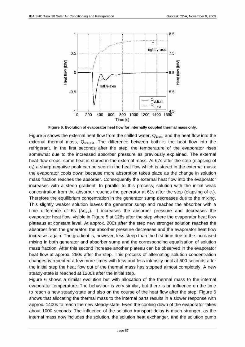
IEA SHC Task 38 Solar Air Conditioning and Refrigeration Subtask C2-A, November 9, 2009
page 87
Figure 6. Evolution of evaporator heat flow for inte rnally coupled thermal mass only.
Figure 5 shows the external heat flow from the chilled water, QE,ext, and the heat flow into the external thermal mass, Qst,E,ext. The difference between both is the heat flow into the refrigerant. In the first seconds after the step, the temperature of the evaporator rises somewhat due to the increased absorber pressure as previously explained. The external heat flow drops, some heat is stored in the external mass. At 67s after the step (elapsing of c1) a sharp negative peak can be seen in the heat flow which is stored in the external mass: the evaporator cools down because more absorption takes place as the change in solution mass fraction reaches the absorber. Consequently the external heat flow into the evaporator increases with a steep gradient. In parallel to this process, solution with the initial weak concentration from the absorber reaches the generator at 61s after the step (elapsing of c2). Therefore the equilibrium concentration in the generator sump decreases due to the mixing. This slightly weaker solution leaves the generator sump and reaches the absorber with a time difference of 6s (∆c1-2). It increases the absorber pressure and decreases the evaporator heat flow, visible in Figure 5 at 128s after the step where the evaporator heat flow plateaus at constant level. At approx. 200s after the step new stronger solution reaches the absorber from the generator, the absorber pressure decreases and the evaporator heat flow increases again. The gradient is, however, less steep than the first time due to the increased mixing in both generator and absorber sump and the corresponding equalisation of solution mass fraction. After this second increase another plateau can be observed in the evaporator heat flow at approx. 260s after the step. This process of alternating solution concentration changes is repeated a few more times with less and less intensity until at 500 seconds after the initial step the heat flow out of the thermal mass has stopped almost completely. A new steady-state is reached at 1200s after the initial step. Figure 6 shows a similar evolution but with allocation of the thermal mass to the internal evaporator temperature. The behaviour is very similar, but there is an influence on the time to reach a new steady-state and also on the course of the heat flow after the step. Figure 6 shows that allocating the thermal mass to the internal parts results in a slower response with approx. 1400s to reach the new steady-state. Even the cooling down of the evaporator takes about 1000 seconds. The influence of the solution transport delay is much stronger, as the internal mass now includes the solution, the solution heat exchanger, and the solution pump
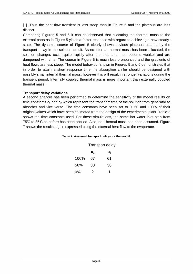
IEA SHC Task 38 Solar Air Conditioning and Refrigeration Subtask C2-A, November 9, 2009
page 88
[1]. Thus the heat flow transient is less steep than in Figure 5 and the plateaus are less distinct. Comparing Figures 5 and 6 it can be observed that allocating the thermal mass to the external parts as in Figure 5 yields a faster response with regard to achieving a new steady-state. The dynamic course of Figure 5 clearly shows obvious plateaus created by the transport delay in the solution circuit. As no internal thermal mass has been allocated, the solution changes occur quite rapidly after the step and then become weaker and are dampened with time. The course in Figure 6 is much less pronounced and the gradients of heat flows are less steep. The model behaviour shown in Figures 5 and 6 demonstrates that in order to attain a short response time the absorption chiller should be designed with possibly small internal thermal mass, however this will result in stronger variations during the transient period. Internally coupled thermal mass is more important than externally coupled thermal mass. Transport delay variations A second analysis has been performed to determine the sensitivity of the model results on time constants c1 and c2 which represent the transport time of the solution from generator to absorber and vice versa. The time constants have been set to 0, 50 and 100% of their original values which have been estimated from the design of the experimental plant. Table 2 shows the time constants used. For these simulations, the same hot water inlet step from 75°C to 85°C as before has been applied. Also, no t hermal mass has been assumed. Figure 7 shows the results, again expressed using the external heat flow to the evaporator.
Table 2. Assumed transport delays for the model.
Transport delay
c1 c2
100% 67 61
50% 33 30
0% 2 1

IEA SHC Task 38 Solar Air Conditioning and Refrigeration Subtask C2-A, November 9, 2009
page 89
Figure 7. Evolution of evaporator heat flow for diff erent transport delay times.
It is visible that the transport delay has a significant influence on the model performance. Without a transport delay, the new steady-state is reached at approx. 200s after the step. With a transport delay of 50% (which corresponds to about half a minute) it takes approx. 500s, e.g. more than double the time to reach it. For the assumed 100% of transport delay (around 1 minute) it takes approx. 900s or more than four times as long. Also, with 100% transport delay, the transient period is not only longer but also quite different in its course. After the elapsing of each transport delay constant, a change in heat flow can be observed in a repeated pattern. The pattern consists of a small change and a larger change following each other which is due to the repetitive change in solution mass fraction as previously explained. The changes become less intensive with time and after approx. 12 delay times the new steady-state is reached. In a real absorption chiller the transport delay is determined by the flow rate of the solution. The model results in Figure 7 show that a significantly faster return to steady-state can be achieved if the flow rate of the solution is high and the transport delays are small.
Experimental verification In Part 1 of this paper, we showed a first comparison of the simulated generator outlet temperature using experimentally measured inlet and outlet temperatures to measured data [1]. In this second part the comparison is also done similarly for the evaporator and absorber. Flow rates and inlet temperatures of the external flows are taken as input data to the simulation model. All internal parameters, the heat flows, and the outlet temperatures of the external flows are simulated. Figure 8 shows measured inlet and outlet temperatures of the chilled water together with the simulated outlet temperature; Figure 9 shows the same for the cooling water through absorber/condenser. The constant simulation parameters for the experimental verification can be found in the Appendix.

IEA SHC Task 38 Solar Air Conditioning and Refrigeration Subtask C2-A, November 9, 2009
page 90
Figure 8. Simulated external evaporator temperatures using experimentally measured input data.
Figure 9. Simulated external absorber temperatures u sing experimentally measured input data.
Both figures show that the dynamic behaviour including small oscillations is in very good agreement. As discussed in part I, the temperature levels are not reproduced satisfactorily because the thermodynamic steady state model is a very coarse one only. This is tolerated because the focus is laid on the dynamics. In Figure 8, the dynamics are being reproduced very well with only a slight delay of 10s between course of the two temperatures. Figure 9 shows a slightly worse agreement for the cooling water temperatures, with simulated values being approx. 25s ahead of measured ones. Also shown in Figure 9 is the simulated outlet temperature of the absorber, tAo,sim, for which no measured data was available. We want to emphasize that no tuning of the dynamic parameters has been performed up to now: the dynamic response seems to be very robust according to the sensitivity analysis which has been shown before.

IEA SHC Task 38 Solar Air Conditioning and Refrigeration Subtask C2-A, November 9, 2009
page 91
Conclusions In this paper, the performance of a dynamic model for absorption chillers has been investigated. General model functionality is demonstrated and the thermodynamics have been found to be consistent with reality. A sensitivity analysis has been performed on external and internal heat exchange related thermal mass. The analysis shows that an increase in both external and internal thermal mass results in a slower response to the step change but also in smaller heat flow oscillations during the transient period. Also, the thermal mass has been found to influence the heat flow transients more significantly if allocated internally. A time difference of 200s for reaching the steady state (response time) was observed between a complete internal and external allocation of thermal mass. The transport delay in the solution cycle has been found to influence both the response time and the transients of the heat flow. A smaller transport delay leads to significantly faster response. Assuming half the value of the real transport delay in the absorption chiller leads to a 33% reduction of response time. The comparison with experimental data shows that the dynamic agreement between experiment and simulation is very good with dynamic temperature deviations between 10 and 25s. The total time to achieve a new steady-state after a 10K input temperature step amounts to approximately 15 minutes for the experimental chiller. Compared to this, the present dynamic deviations of the model are in the magnitude of approximately 1 to 3%. Steady-state results are being reproduced with temperature deviations between 0.7 and 3.5K in the model. Accuracy in this respect, however, was not the aim of the present study. The dynamic simulation model presented in this paper is a useful tool in the overall design process of absorption chillers. Technical changes in the construction of an existing absorption chiller model can be tested quickly and easily by incorporating the design changes in the model. Also, new chiller designs can be tested on their performance without the need to build a prototype. The model also allows the identification of transfer functions and control parameters of absorption chillers without the need to perform experiments. The model has been designed for the Phoenix 10kW chiller but can easily be adapted to other LiBr/water absorption chillers if the required design data of these chillers are available.

IEA SHC Task 38 Solar Air Conditioning and Refrigeration Subtask C2-A, November 9, 2009
page 92
Appendix
Table 3. Constant parameters of the dynamic model.
No. Constants Unit Value Description
1 )( pcr kJkg-1 2450 Evaporation enthalpy of water
2 )( pcl kJkg-1 272 Solution enthalpy of LiBr/water solution
3 ( ) extEUA , kWK-1 2.9 External heat transfer coefficient value of evaporator
4 ( ) extCUA , kWK-1 5.2 External heat transfer coefficient value of condenser
5 ( ) extGUA , kWK-1 4.0 External heat transfer coefficient value of generator
6 ( ) extAUA , kWK-1 3.2 External heat transfer coefficient value of absorber
7 ( ) int,EUA kWK-1 3.9 Internal heat transfer coefficient value of evaporator
8 ( ) int,CUA kWK-1 8.7 Internal heat transfer coefficient value of condenser
9 ( ) int,GUA kWK-1 4.3 Internal heat transfer coefficient value of generator
10 ( ) int,AUA kWK-1 3.2 Internal heat transfer coefficient value of absorber
11 wsolm ,& kgs-1 0.0559 Mass flow of weak solution
12 hwm& kgs-1 0.3322 Mass flow of hot water
13 cwm& kgs-1 0.7462 Mass flow of cooling water
14 chwm& kgs-1 0.808 Mass flow of chilled water
15 At m² 4.9*10-4 Cross area of solution tube
16 h m 0.1 height between solution outlet at generator and inlet at absorber
17 startGsolstM ,,, kg 0.24 Initial condition of accumulated solution in generator sump
18 startAsolstM ,,, kg 0.19 Initial condition of accumulated solution in absorber sump
19 ς - 2100 Resistance coefficient of solution heat exchanger and piping
20 c1 - 67, 2 time constant for solution flow from generator to absorber
21 c2 - 61, 1 time constant for solution flow from absorber to generator
22 ( )extEpMc,
kJK-1 6.8 Cumulated heat capacity of evaporator, external
23 ( )extCpMc,
kJK-1 6.4 Cumulated heat capacity of condenser, external
24 ( )extGpMc,
kJK-1 9.0 Cumulated heat capacity of generator, external
25 ( )extApMc,
kJK-1 9.0 Cumulated heat capacity of absorber, external
26 ( )int,EpMc kJK-1 38.4 Cumulated heat capacity of evaporator, internal
27 ( )int,CpMc kJK-1 38.2 Cumulated heat capacity of condenser , internal
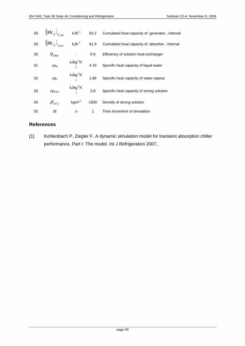
IEA SHC Task 38 Solar Air Conditioning and Refrigeration Subtask C2-A, November 9, 2009
page 93
References [1] Kohlenbach P, Ziegler F. A dynamic simulation model for transient absorption chiller
performance. Part I: The model. Int J Refrigeration 2007,
28 ( )int,GpMc kJK-1 82.2 Cumulated heat capacity of generator , internal
29 ( )int,ApMc kJK-1 81.9 Cumulated heat capacity of absorber , internal
30 SHXη - 0.9 Efficiency of solution heat exchanger
31 cpw kJkg-1K-
1 4.19 Specific heat capacity of liquid water
32 cpv kJkg-1K-
1 1.86 Specific heat capacity of water vapour
33 cpsol,s kJkg-1K-
1 3.8 Specific heat capacity of strong solution
34 ssol ,ρ kgm³-1 1600 Density of strong solution
35 ∆t s 1 Time increment of simulation

IEA SHC Task 38 Solar Air Conditioning and Refrigeration Subtask C2-A, November 9, 2009
page 94
IEA SHC Task 38 Solar Air Conditioning and Refrigeration Subtask C2-A, November 9, 2009
page 95
Conclusion
In this report the new development concerning simulation tools for solar cooling are
presented. First are presented the most commonly used simulation tools in the domain of
solar air conditioning. It was shown that most of simulation tools requires high knowledge of
the simulated process as well as internal development for each project, except some simple
simulation tools with predefined configurations and fixed boundaries. Most of simulation
environment used in each research group in the solar cooling domain are internally
developed and used. In the commercially available detailed softwares; the models of the
solar installation are widely used as in found in the libraries, however the model of the
cooling process itself are usually re-developed by the users.
New development of solar cooling models and their validation are then presented. A detailed
desiccant air handling unit powered by heat pipe vacuum tube collectors is developed and
implemented in SPARK. The model of the unit showed good accuracy on a component level
and on a system level under different operating conditions. The supply conditions of the air
handling unit are estimated with good accuracy as well as the potential of solar energy in the
desiccant cooling process. The transient behaviour of the collector is very well predicted by
the model. A transient model of the desiccant wheel is also developed and experimentally
validated. The model calculates the evolution of the temperature and humidity ratio of the air
across the wheel and at its outlet. It gives also a good estimation of the mean air outlet
conditions of the desiccant wheel.
A transient detailed model of a Li/Br absorption chiller is developed. The model is
experimentally validated and is capable to predict the transient behaviour of the chiller. The
comparison with experimental data shows that the dynamic agreement between experiment
and simulation is very good with dynamic temperature deviations between 10 and 25 s The
dynamic simulation model presented is a useful tool in the overall design process of
absorption chillers. Technical changes in the construction of an existing absorption chiller
model can be tested quickly and easily by incorporating the design changes in the model.