tarek elkhoraibi...tarek elkhoraibi department of civil and environmental engineering university of...
TRANSCRIPT

PACIFIC EARTHQUAKE ENGINEERING RESEARCH CENTER
PEER 2007/101JULY 2007
Generalized Hybrid Simulation Framework for Structural Systems Subjected to Seismic Loading
Tarek Elkhoraibi
and
Khalid M. Mosalam
University of California, Berkeley

Generalized Hybrid Simulation Framework for Structural Systems Subjected to Seismic Loading
Tarek Elkhoraibi Department of Civil and Environmental Engineering
University of California, Berkeley
Khalid M. Mosalam Department of Civil and Environmental Engineering
University of California, Berkeley
PEER Report 2007/101 Pacific Earthquake Engineering Research Center
College of Engineering University of California, Berkeley
July 2007

iii
ABSTRACT
A new hybrid simulation system (HSS), namely nees@berkeley, developed at the University of
California, Berkeley (UCB), is presented in this study. Validation of the HSS is sought through
testing steel cantilever columns with predictable structural response that is verifiable by purely
numerical simulation of the experiment.
Two procedures are developed and implemented in the HSS with the aim of enhancing
the accuracy and reliability of the pseudo-dynamic test results. The first procedure is a feed-
forward error compensation scheme that aims at correcting the experimental systematic error in
executing the displacement command signal. The second procedure employs mixed variables
with mode switching between displacement and force controls. Two experimental test structures
are considered in this study to demonstrate different aspects of the procedures developed in the
HSS: 1. Reinforced concrete frames with and without unreinforced masonry infill walls, and
2. Wood shear walls of the first story of a two-story wood house over a garage.
The structural performance of the two test structures under seismic loading is evaluated
using the developed HSS. The two test structures have the common feature of being large
substructures of shaking table experiments and, accordingly, a comprehensive comparative study
is conducted between the test results of the two testing methods.

iv
ACKNOWLEDGMENTS
This work made use of Pacific Earthquake Engineering Research Center Shared Facilities
supported by the Earthquake Engineering Research Centers Program of the National Science
Foundation under award number EEC-9701568.
The financial support for this project, provided by the National Science Foundation under
NSF Contract No. CMS 0116005, is gratefully acknowledged. The reinforcing bars were donated
by Mr. Thomas R. Tietz, former Western Regional Manager of the Concrete Reinforcing Steel
Institute (CRSI).

v
CONTENTS
ABSTRACT.................................................................................................................................. iii
ACKNOWLEDGMENTS ........................................................................................................... iv
TABLE OF CONTENTS ..............................................................................................................v
LIST OF FIGURES ..................................................................................................................... ix
LIST OF TABLES .......................................................................................................................xv
1 INTRODUCTION .................................................................................................................1
1.1 General ............................................................................................................................1
1.2 Scope and Objectives ......................................................................................................2
1.3 Contributions...................................................................................................................4
1.4 Outline.............................................................................................................................4
2 BACKGROUND....................................................................................................................7
2.1 Comparison of Experimental Methods ...........................................................................7
2.2 Development of HS Experimental Method.....................................................................8
2.3 Integration Algorithms..................................................................................................10
2.4 HS of Stiff Structural Systems ......................................................................................13
2.5 Summary .......................................................................................................................14
3 HYBRID SIMULATION SYSTEM ..................................................................................17
3.1 HSS Overview...............................................................................................................17
3.2 Structural Laboratory ....................................................................................................18
3.2.1 Reconfigurable Reaction Walls (RRW)............................................................18
3.2.2 Actuators ...........................................................................................................21
3.3 ScramNet.......................................................................................................................21
3.4 Structural Test System ..................................................................................................21
3.4.1 PIDF Control.....................................................................................................22
3.4.2 Program Source in STS.....................................................................................23
3.5. xpc Target .......................................................................................................................25
3.6 Pacific Instruments Data-Acquisition System ..............................................................27
3.7 MATLAB Environment ................................................................................................28
3.8 Operation Sequence in HSS..........................................................................................29

vi
3.9 Validation of HSS .........................................................................................................31
3.10 Summary .......................................................................................................................35
4 TEST STRUCTURE A .......................................................................................................37
4.1 ST Test Structure ..........................................................................................................37
4.2 Strong Motion Selection ...............................................................................................38
4.3 Physical Substructures in HS ........................................................................................42
4.4 RC Frame Design..........................................................................................................44
4.5 Instrumentation ............................................................................................................46
4.6 Construction and Material Properties............................................................................50
4.7 Experimental Setup Design...........................................................................................50
4.7.1 Reaction Wall Design and Actuator Selection..................................................50
4.7.2 Setup on Strong Floor .......................................................................................54
4.8 Experimental Setup Implementation.............................................................................54
4.8.1 Construction of RRW........................................................................................55
4.8.2 Attachment of Actuator to RRW ......................................................................55
4.8.3 Attachment of Test Substructures to Strong Floor............................................55
4.8.4 Installation of Loading Apparatus.....................................................................58
4.9 HS Idealization of Test Structure..................................................................................60
4.10 Governing Equations of Motion and Parameters ..........................................................61
4.10.1 Mass Matrix ......................................................................................................62
4.10.2 Damping Matrix ................................................................................................63
4.10.3 Stiffness Matrix.................................................................................................63
4.11 Initial Stiffness Estimation for Physical Substructures.................................................64
4.12 RC Slab Stiffness Estimation........................................................................................66
4.12.1 Theoretical In-Plane Stiffness of RC Slab ........................................................66
4.12.2 Experimental In-Plane Stiffness for RC Slab ...................................................67
4.13 Parameters of Equations of Motion...............................................................................69
4.14 Integration Time-Step Estimation .................................................................................71
4.15 Summary .......................................................................................................................72
5 TEST STRUCTURE B........................................................................................................75
5.1 ST Test Structure ..........................................................................................................75
vii
5.2 Test Structure Design....................................................................................................76
5.3 Strong Motion Selection ...............................................................................................77
5.4 Test Structure in HS......................................................................................................80
5.4.1 Idealization........................................................................................................80
5.4.2 Experimental Setup ...........................................................................................80
5.4.3 Instrumentation .................................................................................................82
5.5 Governing Equation of Motion and Parameters............................................................85
5.6 Summary .......................................................................................................................86
6 NEW ADVANCES IN HYBRID SIMULATION.............................................................87
6.1 Integration Algorithm in DC.........................................................................................87
6.2 Feed-Forward Error Compensation in DC....................................................................90
6.2.1 Test Rate ...........................................................................................................90
6.2.2 Error Prediction.................................................................................................91
6.2.3 Feed-Forward Error Compensation...................................................................93
6.3 Mixed-Variables Control in HS ....................................................................................95
6.3.1 FC Integration Algorithm..................................................................................96
6.3.2 Extension to Mixed-Variables Control .............................................................98
6.4 Numerical Evaluation of FC Algorithm......................................................................102
6.5 Implementation Strategies of Mixed-Variables Control .............................................105
6.5.1 Secant Stiffness Estimation.............................................................................105
6.5.2 Mode-Switch Decision Implementation .........................................................108
6.5.3 Practical Iterative Solution..............................................................................110
6.6 Summary .....................................................................................................................112
7 APPLICATIONS OF DEVELOPED HYBRID SIMULATION PROCEDURES......113
7.1 Feed-Forward Error Compensation.............................................................................113
7.1.1 Calibration Parameter Evaluation ...................................................................113
7.1.2 Experimental Results ......................................................................................116
7.2 Mixed-Variables Control ............................................................................................116
7.2.1 Structural States ..............................................................................................117
7.2.2 Mode-Switch Decision Making ......................................................................118
7.2.3 Experimental Results ......................................................................................121
viii
7.3 Procedure Combination...............................................................................................122
7.4 Summary .....................................................................................................................125
8 STRUCTURAL EVALUATION AND COMPARISONS.............................................127
8.1 Test Structure A: Phase S-1 .......................................................................................127
8.1.1 Force-Displacement Behavior.........................................................................128
8.1.2 URM Infill Wall Contribution ........................................................................132
8.2 Comparison to ST Experiment: Phase S-1.................................................................134
8.2.1 Force-Displacement Behavior.........................................................................134
8.2.2 URM Infill Wall Contribution ........................................................................143
8.3 Test Structure A: Phases S-2 and S-3 .........................................................................147
8.4 Comparisons to ST Experiments: Phases S-2 and S-3...............................................152
8.5 Contribution of Upper Stories.....................................................................................157
8.6 Test Structure B ..........................................................................................................165
8.6.1 Force-Displacement Behavior.........................................................................165
8.6.2 Comparison to ST Experiment........................................................................168
8.7 Summary .....................................................................................................................172
9 SUMMARY, CONCLUSIONS, AND FUTURE WORK ..............................................175
9.1 Summary .....................................................................................................................175
9.2 Conclusions.................................................................................................................176
9.3 Future Work ................................................................................................................178
REFERENCES...........................................................................................................................181
APPENDIX A: SPREADSHEET FOR CONFIGURING REACTION WALL................189
A.1 Background .................................................................................................................189
A.2 Application to Present Test Setup...............................................................................190
APPENDIX B: EXACT SOLUTION FOR BILINEAR STIFFENING SDOF .................195
APPENDIX C: BOUC-WEN MODEL DESCRIPTION AND CALIBRATION ..............197
C.1 Description ..................................................................................................................197
C.2 Calibration...................................................................................................................199

ix
LIST OF FIGURES
Fig. 1.1 Overview of study program..........................................................................................3
Fig. 1.2 Overview of hybrid simulation experimental program ................................................6
Fig. 3.1 Control room and HSS................................................................................................18
Fig. 3.2 HSS architecture .........................................................................................................19
Fig. 3.3 Concrete geometry of typical RRW unit (1"=25.4 mm) ............................................20
Fig. 3.4 STS host PC................................................................................................................23
Fig. 3.5 PIDF controls of displacement (DC) and force (FC) in STS......................................24
Fig. 3.6 Available program sources in STS .............................................................................24
Fig. 3.7 Function generator in STS ..........................................................................................25
Fig. 3.8 Simulink model for xPC target ...................................................................................26
Fig. 3.9 Expansion of operation block in Simulink model for xPC target...............................27
Fig. 3.10 Calibration of sensors in the Pacific Instruments data-acquisition system.................28
Fig. 3.11 Operation sequence in HS ..........................................................................................30
Fig. 3.12 Steel specimens design and setup in structural laboratory .........................................32
Fig. 3.13 Idealized model for HS validation structure...............................................................33
Fig. 3.14 Structural response of physical substructures 1C (left) and 2C (right) ......................34
Fig. 3.15 Validation of HSS.......................................................................................................34
Fig. 4.1 Five-story prototype and one-story ST structures (Hashemi and Mosalam 2007).....38
Fig. 4.2 Response spectra with 5% damping for selected ground motions
(Hashemi and Mosalam 2007)....................................................................................39
Fig. 4.3 Filtering of acceleration time history of ST output signal for TAR level 2 ...............41
Fig. 4.4 Chronological order of events for test structure A .....................................................42
Fig. 4.5 Test structures in HS...................................................................................................43
Fig. 4.6 Infilled frame reinforcement (bare frame is similar without URM infill wall
and grade beam) (1'=304.8 mm, 1"=25.4 mm)...........................................................45
Fig. 4.7 Design details of RC frames (1'=304.8 mm, 1"=25.4 mm) ........................................46
Fig. 4.8 Strain gages numbering on reinforcing steel bars in RC frames ................................47
Fig. 4.9 Numbered displacement transducers on URM infilled RC frame..............................48
Fig. 4.10 Accelerations at faster rate execution, LPB-9 at 20 times slower than real time .......49

x
Fig. 4.11 Out-of-plane drift measurements in TAR-6 frame F2B, phase S-1............................50
Fig. 4.12 Construction of RC frames .........................................................................................51
Fig. 4.13 Strength gain with time for concrete compressive strength of tested cylinders .........52
Fig. 4.14 A 220-kip (979 kN) actuator mounted on RRW ........................................................53
Fig. 4.15 Design spreadsheet output for used RRW (1 ft = 304.8 mm, 1 kip = 4.448 kN) .......54
Fig. 4.16 Test setup on strong floor for test structure A (1'=304.8 mm, 1"=25.4 mm,
1 kip = 4.448 kN)........................................................................................................56
Fig. 4.17 Construction of RRW .................................................................................................57
Fig. 4.18 Installation of actuator at desired height.....................................................................57
Fig. 4.19 Loading apparatus mounted on RC bare frame ..........................................................58
Fig. 4.20 Details of loading apparatus for test structure A (1"=25.4 mm) ................................59
Fig. 4.21 Idealizations of test frame into a number of DOF ......................................................61
Fig. 4.22 Idealized test structure in phase S-1 (see Fig. 1.2) .....................................................61
Fig. 4.23 Mass allocation by tributary areas ..............................................................................62
Fig. 4.24 Pull-back test setup .....................................................................................................65
Fig. 4.25 Restoring force versus lateral displacement of URM infilled RC frame from
preliminary run (1 kip/in. = 0.175 kN/mm)................................................................66
Fig. 4.26 RC slab stiffness estimation (not to scale)..................................................................67
Fig. 4.27 Differential drift in pseudo-dynamic test between F1I and F2B as function of
theoretical in-plane stiffness of RC slab.....................................................................68
Fig. 4.28 Differential drift in dynamic (ST) tests against applied maximum lateral
displacement ...............................................................................................................69
Fig. 4.29 Mode shapes for test structure A in phase S-1 ...........................................................70
Fig. 4.30 Comparison of response for TAR-2 using different integration time steps Δt in
HS ...............................................................................................................................72
Fig. 5.1 Two-story wood house over garage on ST .................................................................76
Fig. 5.2 Wood house first-floor plan........................................................................................77
Fig. 5.3 Wood house elevation views ......................................................................................78
Fig. 5.4 Design details of wood house .....................................................................................79
Fig. 5.5 Blocking used to brace shear-wall framing of test structure B...................................79
Fig. 5.6 Test setup and instrumentation on strong floor for test structure B (1'=304.8 mm,
1"=25.4 mm)...............................................................................................................81

xi
Fig. 5.7 HS physical substructure for test structure B .............................................................82
Fig. 5.8 Loading frame for test structure B (1'=304.8 mm, 1"=25.4 mm)...............................83
Fig. 5.9 Vertical force variation in post-tensioned steel rods in LPG-6 ..................................84
Fig. 5.10 Displacement time history for preliminary test ..........................................................84
Fig. 5.11 Sliding at base of shear walls in preliminary test .......................................................84
Fig. 5.12 Out-of-plane drift of north shear wall in preliminary test ..........................................85
Fig. 6.1 Flowchart of DC algorithm.........................................................................................89
Fig. 6.2 Correlation relationship between error cciEr and actuator velocity for test
structure B...................................................................................................................93
Fig. 6.3 Error remainder (difference between recorded and predicted error values) for test
structure B...................................................................................................................94
Fig. 6.4 Different lumped spring–mass systems ......................................................................97
Fig. 6.5 Flowchart of FC algorithm .........................................................................................99
Fig. 6.6 Flowchart for integration algorithm with mixed-variables control without mode
switch (DC for flexible DOF and FC for stiff DOF) ................................................100
Fig. 6.7 Flowchart for integration algorithm with mode switch between DC and FC for
SDOF system............................................................................................................101
Fig. 6.8 Applied force and considered system for numerical evaluation of FC algorithm....103
Fig. 6.9 Nonlinear elastic response using Menegotto-Pinto model ( IS kk =θ ) ...................103
Fig. 6.10 Parametric study of FC and DC algorithms using nonlinear elastic SDOF
systems......................................................................................................................105
Fig. 6.11 Schematic representation of secant stiffness estimation at time step i +1 and
iteration j .................................................................................................................107
Fig. 6.12 Example results from test structure B for estimation of secant stiffness..................107
Fig. 6.13 Mode-switch decision-making scheme.....................................................................109
Fig. 6.14 Considered stiffening bilinear elastic system for numerical evaluation...................110
Fig. 6.15 Parametric study of mode-switch algorithm using bilinear elastic SDOF
systems......................................................................................................................111
Fig. 7.1 Correlation relationship between error cciEr and actuator velocity..........................115
Fig. 7.2 Feed-forward error compensation results .................................................................117
Fig. 7.3 Typical force-deformatiion response for test structure B .........................................118

xii
Fig. 7.4 FC/DC mode-switch criteria for application example (test structure B)..................119
Fig. 7.5 Mode-switch decision-making scheme for test structure B......................................120
Fig. 7.6 Results of mixed-variables algorithm with mode switch for HS on test
structure B.................................................................................................................123
Fig. 7.7 Results of mixed-variables algorithm with mode switch for HS on test
structure A ................................................................................................................124
Fig. 7.8 Possible incorporation of two developed procedures in HS.....................................124
Fig. 8.1 Total base shear versus lateral displacement for test structure A, phase S-1,
TAR-2 to TAR-6 (1 kip/in.= 0.175 kN/mm) ............................................................130
Fig. 8.2 Total base shear versus lateral displacement for test structure A, phase S-1,
DUZ-7 to DUZ-9-2 (1 kip/in.= 0.175 kN/mm) ........................................................131
Fig. 8.3 Cracking patterns of URM infill wall in test structure A, phase S-1........................131
Fig. 8.4 Contribution of URM infill wall and RC frames to restoring forces........................133
Fig. 8.5 Total base shear versus lateral displacement comparisons for test structure A,
phase S-1 (1 kip/in.=0.175 kN/mm) .........................................................................136
Fig. 8.6 DUZ-7 comparisons for test structure A, phase S-1.................................................138
Fig. 8.7 Cracking patterns developed in URM infill wall in HS and ST experiments
(shaded areas indicate dislocated parts of wall) .......................................................139
Fig. 8.8 Deformation of URM infill wall and bounding RC frame .......................................140
Fig. 8.9 Peak global responses in HS and ST experiments....................................................141
Fig. 8.10 Displacement time histories for TAR-6....................................................................142
Fig. 8.11 Total base shear time histories for TAR-6................................................................142
Fig. 8.12 URM infill wall contributions to restoring forces in HS and ST experiments .........143
Fig. 8.13 Shear force versus shear strain of URM infill wall ..................................................145
Fig. 8.14 Estimation of shear strain from diagonal measurements ( 1Δ and 2Δ ) ....................145
Fig. 8.15 URM infill wall sliding on bottom interface with respect to surrounding RC
frame, TAR-6............................................................................................................146
Fig. 8.16 Observed damage in RC frame at beginning of phase S-2.......................................147
Fig. 8.17 Peak lateral displacement and peak total base shear for phases S-2 and S-3 ...........148
Fig. 8.18 Total base shear versus lateral displacement for test structure A, phase S-2 for
level LPB-9-2[2] (1 kip/in.=0.175 kN/mm) .............................................................149

xiii
Fig. 8.19 Observed damage at end of phase S-2......................................................................150
Fig. 8.20 Total base shear versus lateral displacement for test structure A, phase S-3 for
level LPB-9-5[3] (1 kip/in.=0.175 kN/mm) .............................................................151
Fig. 8.21 Observed damage at end of phase S-3......................................................................151
Fig. 8.22 Rotation measurement in RC column-to-footing joint .............................................152
Fig. 8.23 Top (beam-to-column) and bottom (column-to-footing) joint rotations for east
column ......................................................................................................................153
Fig. 8.24 East column deformed shape at end of phase S-3, LPB-10[3] .................................154
Fig. 8.25 Peak lateral displacement and peak total base shear relationships for test
structure A, phase S-2...............................................................................................155
Fig. 8.26 Peak lateral displacement and total base shear relationships for test structure A,
phase S-3...................................................................................................................156
Fig. 8.27 Comparison of observed damage between HS and ST table test structures at
end of phase S-3........................................................................................................157
Fig. 8.28 Schematic representation of test structures for quantifying the contribution of
upper stories..............................................................................................................158
Fig. 8.29 Idealized computational models of test structures for quantifying contribution
of upper stories .........................................................................................................160
Fig. 8.30 Restoring force versus lateral displacement of first-story URM infilled frame .......162
Fig. 8.31 Evaluated fundamental frequencies of vibration in TAR-2 for different
structural systems......................................................................................................163
Fig. 8.32 Evaluated fundamental frequencies of vibration in DUZ-8 for different
structural systems......................................................................................................164
Fig. 8.33 Spectral acceleration of applied strong motions (5% damping ratio) for
quantifying contribution of upper stories .................................................................165
Fig. 8.34 Total base shear versus lateral displacement for HS for test structure B (1
kip/in.=0.175 kN/mm) ..............................................................................................167
Fig. 8.35 Framing-to-sheathing connection schematic of local deformation ..........................168
Fig. 8.36 Deformed shape of wood shear walls at peak lateral displacement .........................168
Fig. 8.37 Total base shear versus first-story lateral displacement for test structure B for
LPG-4 (ST experiment) ............................................................................................169
Fig. 8.38 Displacement time-history comparison for test structure B for LPG-4....................170

xiv
Fig. 8.39 Total base shear time-history comparison for test structure B for LPG-4................170
Fig. 8.40 Displacement time-history comparison for test structure B for LPG-6....................171
Fig. 8.41 Total base shear time-history comparison for test structure B for LPG-6................171
Fig. 8.42 Displacement time history for test structure B for third (last) repetition of
LPG-6 (ST experiment) ............................................................................................172
Fig. A.1 Design spreadsheet input for RRW design...............................................................191
Fig. A.2 Design spreadsheet output for used RRW (1 kip = 4.448 kN, 1 ft = 30.48 mm) .....192
Fig. A.3 Frequency calculation of seven-unit high (210 in. (5334 mm)) RRW.....................193
Fig. B.1 Considered SDOF system.........................................................................................195
Fig. B.2 Typical displacement response of bilinear stiffening undraped SDOF system........196
Fig. C.1 Example of Bouc-Wen model including pinching ...................................................199
Fig. C.2 Bouc-Wen model calibration — TAR-2...................................................................200
Fig. C.3 Bouc-Wen model calibration — DUZ-8 ..................................................................201

xv
LIST OF TABLES
Table 3.1 Actuator characteristics in nees@berkeley ............................................................. 21
Table 3.2 Evaluated parameters for validation of HSS ........................................................... 33
Table 4.1 Ground motion specifications (1 in. = 25.4 mm) .................................................... 38
Table 4.2 Scale factors for different levels of input ground motions...................................... 40
Table 4.3 Physical substructures in HS ................................................................................... 43
Table 4.4 Concrete compressive strength of tested cylinders ................................................. 52
Table 4.5 Expected load and displacement requirements of substructures in test structure
A .............................................................................................................................. 52
Table 4.6 Pull-back test results for substructures of test structure A ...................................... 65
Table 4.7 Values of parameters used in RC slab in-plane stiffness estimation....................... 67
Table 4.8 Estimated parameters for test structure A in phase S-1 .......................................... 70
Table 4.9 Natural frequencies and periods for test structure A in phase S-1 .......................... 71
Table 5.1 Loma Prieta 1989, Los Gatos station strong motion (LPG).................................... 80
Table 5.2 Scale factors for different levels of input ground motion (fault normal) except
as noted.................................................................................................................... 80
Table 5.3 Estimated parameters for HS of test structure B ..................................................... 86
Table 6.1 Varied parameters for numerical evaluation of FC algorithm .............................. 104
Table 6.2 Varied parameters for numerical evaluation of mode-switch and iterative
approach ................................................................................................................ 112
Table 7.1 Calibration parameters for feed-forward error compensation procedure,
Eq. 6.17 ................................................................................................................. 114
Table 8.1 Tangent stiffness evaluation for test structure A, phase S-1 ................................. 129
Table 8.2 URM infill wall contribution to total restoring force............................................ 134
Table 8.3 Tangent stiffness comparisons for test structure A, phase S-1 ............................. 137
Table 8.4 Parameters for quantifying of contribution of upper stories ................................. 161
Table 8.5 Estimated natural periods (sec) for 3 DOF and 15 DOF systems ......................... 161
Table 8.6 Natural periods nT and corresponding spectral accelerations AS ........................ 164
Table B.1 Parameters for bilinear stiffening undamped SDOF system................................. 196
Table C.1 Bouc-Wen model calibration parameters .............................................................. 199

1 Introduction
1.1 GENERAL
Experimental testing methods continue to benefit from technological advances. The George E.
Brown, Jr. Network for Earthquake Engineering Simulation (NEES) was created by the National
Science Foundation with the purpose of promoting research and education in earthquake
engineering. In particular, at the University of California, Berkeley (UCB), a new hybrid
simulation system (HSS), nees@berkeley, was established with major facilities for conducting
pseudo-dynamic (online) experiments. The experimental program in the present study was
designed for the purpose of developing the hybrid simulation (HS) testing method as a powerful
tool for testing structural systems with an emphasis on hybrid systems, which include flexible
and stiff structural elements.
Unreinforced masonry (URM) infill walls are commonly incorporated in buildings
constructed in seismic and non-seismic regions, but their effect on the structural response of the
structural system is often neglected during the design process. While this assumption may be
valid when considering gravity loads, the lateral load resistance of these URM infill walls has a
major effect on the response of the infilled systems, e.g., reinforced concrete (RC) frames, under
seismic loading. The structural behavior of an infilled system is characterized by its hybrid
nature due to the interaction between stiff elements (infill walls) and flexible elements (bounding
frames). Although many research activities have been conducted on frames with infill walls
(Mosalam 1996a, b, Mosalam et al. 1997a–e and Mosalam et al. 1998), the behavior of these
structural systems under seismic loading is not yet well understood, and further experimental and
computational studies are still needed. Moreover, understanding the behavior of these structural
systems beyond the failure of one or more contributing elements, e.g., the URM infill wall, to the

2
lateral load resistance is crucial for the evaluation of structural systems experiencing progressive
collapse under severe dynamic loading, e.g., due to earthquakes.
Timber structures, especially low-rise residential buildings, represent about 80% of the
U.S. market. The seismic vulnerability of these structures was demonstrated during recent
earthquakes in California. In particular, wood-frame buildings with an open front due to tuck-
under parking are characterized by a “soft” (weak) first story. During the 1994 Northridge
earthquake, 24 of the 25 fatalities that were caused by building damage occurred in wood-frame
buildings. Moreover, half or more of the $40 billion in property damage was related to wood-
frame construction. In addition to the soft first story characterizing buildings with tuck-under
parking, their usually asymmetric configuration in plan and irregularity in elevation may bring
about torsional effects when subjected to ground motions (Mosalam et al. 2002; Mosalam and
Mahin 2007). The assessment of the structural performance of this type of buildings under
dynamic loading is therefore of great importance and is needed to identify the weaknesses and
possible methods of enhancing the resistance to earthquake loading.
1.2 SCOPE AND OBJECTIVES
The overall study program, outlined in Figure 1.1, is designed for the purpose of addressing a
number of structural engineering problems. The topics in boxes 1–2, 4–6, 10, 14, and 16 are
considered in Hashemi and Mosalam (2007) and focus on RC structures with URM infill walls
looking to understand their structural response in terms of the interaction between infill walls and
their bounding frames. Moreover, the damage and collapse mechanism is evaluated in Hashemi
and Mosalam (2007), with the aim of developing representative computational models of URM
infill walls and conducting reliability analysis on this type of structures. The topics in boxes 8–9,
13, and 15 are considered in Talaat and Mosalam (forthcoming 2007) and focus on the
progressive collapse of structures and modeling their behavior by improving constitutive
material and damage models and developing element removal algorithms, having the RC frame
structure with URM infill wall as one of the main applications. The scope of this report is
focused on tasks in boxes 3, 7, 11–12, and 17–18 in Figure 1.1. The detailed hybrid simulation
framework designed to investigate these specific tasks is outlined at the end of this chapter in
Figure 1.2.

3
Prototype structure
A1 A2
B1 B2
C1C2
A3 A4
B3 B4
C4
Development and validation of
FE model
Verification of hybrid simulation
with sub-structuring
Development of generalized hybrid simulation framework
Infill-RC frame
interaction
Damage sequence and collapse mechanism
Development of element removal
algorithms
Improvement of RC constitutive material
& damage models
Development of new SAT models
Progressive collapse analysis for RC structures with URM
infill walls
Shake-tabletests
Pseudo-dynamic
tests
Numerical simulations on URM
infill walls
Reliability analysis for performance evaluation of RC structures with
URM infill walls
Development oferror-free
hybrid simulation
Mixed variables (displacement/force) control for flexible/
stiff structures
Error compensation in
displacement control
1
2 3
4 5 67
8 9 10
11 12
14
15 16 1817
Development of element removal
criteria13
Prototype structure
A1 A2
B1 B2
C1C2
A3 A4
B3 B4
C4
Development and validation of
FE model
Verification of hybrid simulation
with sub-structuring
Development of generalized hybrid simulation framework
Infill-RC frame
interaction
Damage sequence and collapse mechanism
Development of element removal
algorithms
Improvement of RC constitutive material
& damage models
Development of new SAT models
Progressive collapse analysis for RC structures with URM
infill walls
Shake-tabletests
Shake-tabletests
Pseudo-dynamic
tests
Pseudo-dynamic
tests
Numerical simulations on URM
infill walls
Reliability analysis for performance evaluation of RC structures with
URM infill walls
Development oferror-free
hybrid simulation
Mixed variables (displacement/force) control for flexible/
stiff structures
Error compensation in
displacement control
1
2 3
4 5 67
8 9 10
11 12
14
15 16 1817
Development of element removal
criteria13
Fig. 1.1 Overview of study program.
The understanding of URM infilled RC systems is sought using HS in phases S-1, S-2,
and S-3, as illustrated in Figure 1.2. Moreover, the idealizations, assumptions, and
approximations inherent in the HS approach using the substructuring technique are evaluated by
drawing a comparison with truly dynamic (shaking-table) benchmark experiments performed on
a similar test structure. The potential of pseudo-dynamic experimentation is explored further
through the development of a number of procedures aimed at increasing the accuracy of the
execution of the experiment. First, the test rate, its implications on the test results, the
experimental error evaluation and possible feed-forward compensation procedure are
investigated in phase P-1 in Figure 1.2. Second, the possibility of performing pseudo-dynamic
experiments in mixed-variables (displacement and force) control with mode-switching
capabilities between the two control modes is explored in phase P-2, as depicted in Figure 1.2.
These procedures are aimed at developing an error-free HS framework applicable to flexible/stiff
structures and implemented in the nees@berkeley HSS. The developed procedures are performed
on two different experimental test structures, namely:

4
1. RC frames with and without URM infill wall (test structure A in this report and referred
to as test structure II in Elkhoraibi and Mosalam (2007)) as substructures of a five-story
infilled RC building; and
2. Wood shear walls (test structure B in this report and referred to as test structure I in
Elkhoraibi and Mosalam (2007)) of the first story of a two-story wood house-over-
garage.
1.3 CONTRIBUTIONS
This study aims toward developing a generalized error-free hybrid simulation framework
implemented within the nees@berkeley test facility. Accordingly, the following are regarded as
the main contributions toward this goal: • A novel implicit force-control algorithm is derived based on the α -method and a
numerical parametric study is conducted to evaluate its validity and accuracy. • Mixed-variables (displacement and force) control is implemented within the hybrid
simulation system with experimental validations on test structures exhibiting flexible/stiff
behaviors. • A comprehensive comparative study is conducted between the truly dynamic (shaking
table) and the pseudo-dynamic (hybrid simulation) testing methods through the testing of
identical structures using both experimental methods.
1.4 OUTLINE
The report is organized into nine chapters. Chapter 1 discusses the motivation of the study, its
scope, objectives, and major contributions, with an overview of the different phases of the
experimental program. A comparison between shaking-table (ST), quasi-static, and pseudo-
dynamic experimental methods is presented in Chapter 2 with a special emphasis on the pseudo-
dynamic method, discussing its advantages and limitations, as well as the numerical-integration
algorithms associated with this type of hybrid simulation approach. The HSS at UCB
nees@berkeley, is presented in Chapter 3, and a description of the operation sequence of the
system is included, as well as a validation experiment conducted on the newly installed HSS.
The design, construction, and instrumentation of the two test structures considered in this study

5
along with the design of their experimental setups are presented in Chapters 4 and 5 for test
structures A and B, respectively. In these chapters, the development of the idealized lumped-
mass model for each test structure and the estimation of key parameters in the governing
equations of motion are discussed in addition to other estimated parameters such as the
numerical-integration time step. In Chapter 6, the algorithmic formulation of the numerical
solution of the governing equations of motion and the implementation of the displacement
control (DC) algorithm are illustrated. Moreover, a procedure allowing for a feed-forward
compensation of the experimental error of the displacement command execution is developed. A
novel implicit force-control (FC) algorithm is derived and evaluated by a numerical parametric
study. The implementation of this FC algorithm in the HSS, with mode switch between force and
displacement control, is considered and several implementation strategies are developed. The FC
algorithm is extended to a mixed formulation where FC may be used for certain degrees of
freedom of the test structure and DC for others. Chapter 7 presents the implementation and
results of the two procedures developed in Chapter 6 (phases P-1 and P-2 in Fig. 1.2) on test
structures A and B. The structural evaluation of test structure A (phases S-1, S-2, and S-3 in Fig.
1.2) and that of test structure B, as well as the comparison of HS and ST experiments are
discussed in Chapter 8. Finally, a summary, major conclusions, and future extensions are
presented in Chapter 9.

6
Shakingtable testphase 1
Shakingtable testphases 2&3
RC Frame No.1
Infilled/Bare F1I/B
RC Frame No.2BareF2B
Hybrid simulation system validation
S-1
F1IF2B
One story RC framewith and without URM infill
+ post-tensioned columns
S-2
F2B
URM infill wall removed after collapse
+ post-tensioned columns
S-3
F2B
No post-tensioningin columns
S = Structural evaluationP = Procedure development
Test rate study/ Error compensation
Mixed variables: force/displacement
control
P-1 P-2
F1B WoodShear walls
Test Structure B
Test Structure A
* * *
*
Shakingtable testphase 1
Shakingtable testphases 2&3
RC Frame No.1
Infilled/Bare F1I/B
RC Frame No.2BareF2B
Hybrid simulation system validationHybrid simulation system validation
S-1
F1IF2B
One story RC framewith and without URM infill
+ post-tensioned columns
S-2
F2B
URM infill wall removed after collapse
+ post-tensioned columns
S-3
F2B
No post-tensioningin columns
S = Structural evaluationP = Procedure development
Test rate study/ Error compensation
Mixed variables: force/displacement
control
P-1 P-2
F1B WoodShear walls
Test Structure B
Test Structure A
* * *
*
* Labeled frames are the physically modeled ones in the hybrid simulation experiments
Fig. 1.2 Overview of hybrid simulation experimental program.

2 Background
In this chapter, different experimental methods of structures subjected to dynamic loading,
particularly those due to ground motion caused by earthquakes, are compared and the HS, i.e.,
pseudo-dynamic experimental method, is described. The development of the method is
summarized and the integration algorithms used to solve the governing equations of motion of
test structures are presented. HS of stiff structures in particular is examined.
2.1 COMPARISON OF EXPERIMENTAL METHODS
Structures subjected to seismic loading exhibit complex behavior, and several experimental
techniques are employed to simulate their response. Purely numerical simulations are based on
assumptions concerning the properties of materials and the behavior of structural elements,
which are inherently uncertain. Experimental techniques are therefore needed to validate the
accuracy of numerical simulation models. These techniques are divided into three main
categories: (1) ST experiments, (2) quasi-static experiments, and (3) pseudo-dynamic
experiments, also known as the online experiments, or HS.
In the ST experiments, the test structure is placed on the seismic simulator that is then
subjected to a recorded strong motion by means of dynamic actuators. While this experimental
technique is truly dynamic, the size of the ST and the capacity of the dynamic actuators,
responsible for applying the strong motion, put limitations on the size of the test structure, the
amplitude of the applied motion, and the accuracy of its implementation. If a small-scale
specimen is used, similitude problems occur and the interpretation of the results becomes
difficult. Note that other dynamic experimental techniques, such as the effective force method,
are developed for the purpose of real-time experiments (Dimig et al. 1999; Shield et al. 2001;
Wu et al. 2007) to alleviate the limitations associated with ST experiments.

8
The quasi-static experiments use static actuators to load the test structure at low speed
with a prescribed load (displacement) time history. This allows testing larger structures than
those that can be tested on the ST under large amplitudes of motion with high fidelity to the
selected input pattern of loads or displacements. However, the equivalent static load or
displacement needs to be defined prior to testing, e.g., by a series of loading/unloading
(sinusoidal) cycles or by numerically solving the equations of motion using step-by-step
numerical-integration algorithms (see Section 2.3) in the case of a defined seismic excitation
with assumed structural parameters that are not entirely known in advance. In particular, while
mass and damping may be estimated with reasonable accuracy, the stiffness of a test structure
exhibiting nonlinear behavior changes as the loading progresses and causes the restoring forces
and deformations to change accordingly. Thus, in general, the calculated loading history to be
applied in quasi-static experiments may not correspond to the actual response of the test structure
if it were tested dynamically.
HS experiments use the governing equations of motion of an equivalent lumped-mass
system of the test structure to solve for the equivalent static load or displacement, but do so
interactively during the experiment by using the readily available (online) force and deformation
information from the test structure. At each integration time step, the displacement is applied on
the test structure and its corresponding restoring-force feedback is measured and used to solve
the next integration time step. This technique inherits the advantages of quasi-static experiments
as well as implementing a much more accurate loading history by benefiting from these online
measurements (feedbacks) and simulations.
2.2 DEVELOPMENT OF HS EXPERIMENTAL METHOD
Since the first development introduced in Takanashi et al. (1975), the pseudo-dynamic method
proved to be a versatile experimental approach and has benefited from technologically improved
hardware and developed integration algorithms and techniques. A U.S.-Japan Cooperative
Earthquake Research Program in the 1980s provided impetus for further development, with
significant research efforts in the U.S. occurring primarily at UCB (Shing and Mahin 1983, 1984,
1985, 1987a, b; Shing et al. 1984) and the University of Michigan, Ann Arbor (McClamroch et
al. 1981; Hanson and McClamroch 1984). Much of this research focused on accuracy
9
verification of this test method and the investigation into the control of certain experimental
intricacies affecting the pseudo-dynamic test.
Comparative testing of pseudo-dynamic and ST methods by Yamazaki et al. (1989)
revealed concerns regarding loading-rate effects and experimental errors. Takanashi and
Nakashima (1987) and Mahin et al. (1989) provide summaries of the early development of the
pseudo-dynamic testing in both Japan and the U.S., respectively, and identify needs for improved
control of hydraulic actuators to limit the inevitable experimental errors. Loading-rate effects
have largely been tolerated compared to uncertainties in small-scale ST tests. However, in some
cases of velocity-dependent behavior, real-time HS is of interest and several research activities
have studied that aspect by performing real-time pseudo-dynamic testing (Nakashima 2001;
Magonette 2001) and by developing integration algorithms suitable for high-speed testing
(Bonelli and Bursi 2004).
Perhaps one of the most important features of HS is substructuring (Dermitzakis and
Mahin 1985; Gawthrop et al. 2005). In this technique, the test structure is divided into physically
modeled and numerically simulated substructures. The numerical simulation is assigned to
elements of the structure with well-understood behavior and the physical modeling is reserved
for the more complex structural elements. Geographically distributed testing is another attractive
feature in the HS testing method that is based on substructuring (Pinto et al. 2002; Mosqueda
2003; Pan et al. 2006; Takahashi and Fenves 2006). In Mosqueda (2003), a bridge is tested with
the columns physically modeled, whereas the deck, which is expected to behave as a rigid
connecting body, is numerically simulated. Furthermore, experimental and computational
substructures are tested in different laboratories (sites) where data exchange between different
simulation sites is achieved via the Internet.
Large-scale pseudo-dynamic experiments have been performed on stiff structures
including masonry walls. A major pseudo-dynamic testing program at the University of
California, San Diego, has been conducted on a five-story full-scale reinforced masonry test
building. Two significant innovations that evolved during this research include the “soft-
coupling” to improve actuator control and the “generalized sequential displacement method” to
generalize pseudo-dynamic testing beyond a single ground motion (Seible et al. 1994a,b, 1996).
At Cornell University, pseudo-dynamic testing has been conducted for the first time on a two-
story infilled steel frame (Mosalam 1996a, 1997c, 1998) and on a two-story infilled RC frame
(Buonopane 1997).

10
2.3 INTEGRATION ALGORITHMS
Numerical-integration algorithms, used to solve the equations of motion, play a major role in HS.
A variety of algorithms exist and may be classified into explicit and implicit methods. Explicit
formulations predict the displacement to be imposed on the test structure as a function of the
information already available from the previous time steps. On the other hand, implicit
formulations require information from the current time step to satisfy the kinematic conditions
imposed on the test structure and the dynamic equilibrium governed by the equations of motion
at the end of the time step; hence an iterative approach is needed. Most of the first-generation HS
testing and research focused on the use of explicit time-integration algorithms (Shing and Mahin
1985). The intention of using HS tests to study the nonlinear seismic behavior of structures led to
an avoidance of implicit techniques. With varying tangent stiffness at each time step, implicit
solutions would require iterations unless reliable prediction of this continuously changing
stiffness is made. Such iterations must be imposed on the test structure and therefore may
introduce unrealistic loading/unloading cycles, one of the drawbacks of quasi-static testing meant
to be avoided with pseudo-dynamic testing.
At this point, let us introduce the governing equations of motion for an idealized lumped-
mass multiple-degree-of-freedom (MDOF) system subjected to an excitation force vector P as
follows:
PKuuCuM =++ (2.1)
where the MDOF system is described by the mass matrix M , damping matrix C , restoring-force
vector KuR = with K as the stiffness matrix of the structure, and the acceleration, velocity,
and displacement vectors are denoted u , u and u , respectively. Notice that the structure is
idealized into a finite number of degrees of freedom (DOF) with lumped masses, which is an
assumption not necessarily applicable for every structure (Shing et al. 1996).
Newmark’s numerical-integration method (Newmark 1959) is presented below as the
most common integration algorithm in structural dynamics. At time 1+it , the equations of motion
are discretized as follows:
1111 ++++ =++ iiii PKuuCuM (2.2)

11
This is supplemented with the following expressions for the discretized displacement and
velocity vectors,
( ) 122
1 21 ++ Δ+−Δ+Δ+= iiiii ttt uuuuu ββ (2.3)
( ) 11 1 ++ Δ+−Δ+= iiii tt uuuu γγ (2.4)
where tΔ is the time step and β and γ are parameters of integration. Making use of
11 ++ = ii KuR , Equation (2.4) and Equation (2.2) are used to estimate the acceleration vector as
follows:
[ ] ( )[ ]{ }iiiii tt uuCRPCMu γγ −Δ+−−Δ+= ++−
+ 1111
1 (2.5)
The application of the above algorithm in the context of pseudo-dynamic experimentation
starts by applying an explicit version of Equation (2.3) to find the predicted displacement, and
after its application on the test structure, the corresponding restoring-force vector 1+iR is
measured. This predictive step is subsequently corrected in an iterative manner using Equations
(2.4)–(2.5) to satisfy equilibrium in Equation (2.2). Based on the values of the parameters β and
γ , the method is defined as an average acceleration approach ( 41=β and 21=γ ) or a linear
acceleration approach ( 61=β and 21=γ ). Both of these approaches are implicit in nature
since the displacement at time 1+it , i.e., 1+iu , is a function of the unknown acceleration 1+iu . Note
that the factor γ introduces artificial numerical damping in the system if taken to be greater than
one half (Dermitzakis and Mahin 1985). The application of explicit integration is limited by
certain conditional stability limits. If 0=β in the Newmark’s numerical-integration method, the
method becomes explicit and combined with 21=γ , the method reduces to the central
difference method. As an example, the condition of convergence for the central difference
method is nt ω2≤Δ where nω is the largest natural frequency of the structure (Chopra 2000).
For MDOF systems, as nω increases, this condition of convergence may prove to be a major
limitation, especially when considering the effect of experimental errors. This situation is very
complicated due to the fact that the experimental errors increase with reduced time steps and
may develop into spurious higher-mode response (Shing and Mahin 1983). For the purpose of
controlling the spurious growth of experimental errors in higher-frequency modes, Shing and

12
Mahin (1983) suggested a modified Newmark explicit method employing artificial numerical
damping with the modal damping ratio increasing proportionally with ntωΔ .
One of the most recognized numerical-integration algorithms was introduced in Hilber et
al. (1977) and Hughes (1983) as the modified Newmark implicit α -method. In this algorithm,
the equations of motion are written in the following form:
( ) 1111 1 ++++ =−+++ iiiii PRRuCuM αα (2.6)
The displacement and velocity vectors are computed from Equations (2.3) and (2.4),
respectively. The introduced parameter α adds dissipation in the form of artificial damping to
the MDOF system and is related to the original parameters in Newmark’s numerical-integration
method β and γ by ( ) 41 2αβ −= and αγ −= 21 . If 0=α , no numerical damping is
introduced and the method reduces to the average acceleration method. This implicit method
leads to the following relationships:
( )[ ] ( ) ( ){ }11
12
21
11
21
++−
+
+−Δ−−−+Δ+Δ
+−Δ+Δ+=
iiiii
iiii
ttt
tt
RuCuCRPCM
uuuu
αγαγβ
β (2.7)
Notice that the right hand side of the above equation is explicit except for the restoring-force
vector 1+iR .
Based on the implicit-explicit method developed by Hughes et al. (1979), Nakashima et
al. (1990) developed an operator-splitting (OS) scheme where the stiffness of the structure is
split into experimental and numerical parts. This method allows the implementation of an
explicit algorithm for the physical substructure and an implicit algorithm for the computational
substructure. Moreover, the operator-splitting scheme ensures an unconditionally stable
numerical solution if the nonlinearity of the physical substructure is of the softening type. Novel
approaches such as the state-space procedure based on the interpolation of the discrete excitation
signals for piecewise convolution integral are combined with the operator-splitting scheme
(Wang et al. 2001). Recent developments include integration algorithms allowing a reliable real-
time implementation of HS (Darby et al. 2001).
13
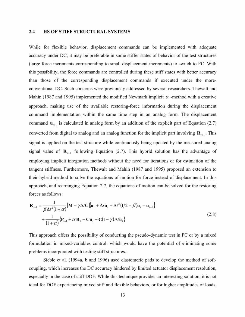
2.4 HS OF STIFF STRUCTURAL SYSTEMS
While for flexible behavior, displacement commands can be implemented with adequate
accuracy under DC, it may be preferable in some stiffer states of behavior of the test structures
(large force increments corresponding to small displacement increments) to switch to FC. With
this possibility, the force commands are controlled during these stiff states with better accuracy
than those of the corresponding displacement commands if executed under the more-
conventional DC. Such concerns were previously addressed by several researchers. Thewalt and
Mahin (1987 and 1995) implemented the modified Newmark implicit α -method with a creative
approach, making use of the available restoring-force information during the displacement
command implementation within the same time step in an analog form. The displacement
command 1+iu is calculated in analog form by an addition of the explicit part of Equation (2.7)
converted from digital to analog and an analog function for the implicit part involving 1+iR . This
signal is applied on the test structure while continuously being updated by the measured analog
signal value of 1+iR following Equation (2.7). This hybrid solution has the advantage of
employing implicit integration methods without the need for iterations or for estimation of the
tangent stiffness. Furthermore, Thewalt and Mahin (1987 and 1995) proposed an extension to
their hybrid method to solve the equations of motion for force instead of displacement. In this
approach, and rearranging Equation 2.7, the equations of motion can be solved for the restoring
forces as follows:
( ) [ ] ( ){ }
( ) ( ){ }iiii
iiiii
t
tttt
uCuCRP
uuuuCMR
Δ−−−++
+
−−Δ+Δ+Δ++Δ
=
+
++
γαα
βγαβ
11
1
211
1
1
12
21
(2.8)
This approach offers the possibility of conducting the pseudo-dynamic test in FC or by a mixed
formulation in mixed-variables control, which would have the potential of eliminating some
problems incorporated with testing stiff structures.
Sieble et al. (1994a, b and 1996) used elastomeric pads to develop the method of soft-
coupling, which increases the DC accuracy hindered by limited actuator displacement resolution,
especially in the case of stiff DOF. While this technique provides an interesting solution, it is not
ideal for DOF experiencing mixed stiff and flexible behaviors, or for higher amplitudes of loads,

14
where the technique used to install the pads, employing a friction connection, becomes highly
nonlinear and may affect the control accuracy especially at these higher load amplitudes.
Pan (2004) and Pan et al. (2005) tested a high-damping rubber bearing under seismic
loading using mixed displacement-force control to apply the bearing axial load. Force control
was used for loading in compression, which is associated with a high stiffness, and DC was used
for loading in tension, which is associated with a much lower stiffness. The force command in
the former case was calculated as the product of the calculated displacement command and a
predetermined constant stiffness, assuming elastic response in compression. While this solution
is suitable for a linear elastic structure, for a structure with nonlinear stiffness, the solution is not
valid.
2.5 SUMMARY
Different experimental methods developed for the simulation of structural behavior under
seismic loading are compared, with a focus on the advantages and disadvantages of the hybrid
simulation testing. The development of hybrid simulation is summarized in terms of its earlier
development, the problems it encounters, and the major efforts conducted to overcome these
obstacles. The hybrid simulation testing method for testing the seismic performance of structures
offers a number of advantages, summarized as follows: • Allows testing larger-scale test structures than on the shaking table. • Allows testing physical substructures experimentally while modeling other parts of the
structure numerically. • Offers the possibility of running simulations slower than real time to allow better
monitoring of structural degradation. • Offers the possibility of geographically distributed testing.
On the other hand, the hybrid simulation testing method faces some problems: • Testing stiff structural systems remains a challenge. • Rate-sensitive materials need to be tested in real or close to real time, although several
efforts have been made in that regard.
To lay out the foundation of the hybrid simulation method, the equations of motion of a
structural system subjected to dynamic loading are presented. Newmark’s numerical-integration

15
method is presented as an example of the most widely used numerical-integration algorithms to
solve the equations of motion during hybrid simulation. Finally, the development of new
integration algorithms and novel techniques intended for the implementation in hybrid
simulation are discussed including the treatment of stiff structural systems.

3 Hybrid Simulation
The HSS at [email protected] consists of several components interconnected to allow for an
efficient implementation of the online experimental technique with flexibility in designing the
test setup. This chapter presents the different components of this particular HSS, its inner and
interconnecting structures, and the testing possibilities such a system may offer. The newly
installed GSS is then validated for the purpose of ensuring its proper functionality. for this
validation, a pseudo-dynamic experiment is designed with a numerically reproducible structural
behavior of the test specimens where experimental results using the HSS are validated against
pure numerical simulation.
3.1 HSS OVERVIEW
The main components of the HSS used in the present study are shown in Figure 3.1. Each
component is described in terms of its function and connections with the other constituents of the
system. The main components are as follows:
1. Structural laboratory
2. ScramNet
3. Structural Test System (STS)
4. xPC target
5. Pacific Instruments data-acquisition system
6. MatLab environment
The architecture of the HSS is illustrated further in figure 3.2, where data exchange is identified.
A detailed description of each component is presented in subsequent sections.

18
PI Data Acquisition
MatLab and xPC
STS Controller
Control Room
ObservationWindow toStructuralLaboratory
PI Data Acquisition
MatLab and xPC
STS Controller
Control Room
ObservationWindow toStructuralLaboratory
Fig. 3.1 Control room and HSS.
3.2 STRUCTURAL LABORATORY
The structural laboratory provides the experimental site for testing the specimens using
reconfigurable reaction walls (RRW). It includes the strong floor as well as the necessary
hydraulic actuator system for loading the experimental substructures.
3.2.1 Reconfigurable Reaction Walls (RRW)
The RRW is constructed by assembling a number of precast high-strength RC units of box-
section type. These units are post-tensioned using high-strength steel rods to work in unison as a
single or multiple reaction system fixed to the laboratory strong floor. The stiffness and
fundamental frequencies of the RRW are evaluated experimentally for the configuration used in
this study and confirmed for no possible interaction with the dynamics of the studied test
structures (Mosalam and Elkhoraibi 2004). Upon assembling the RRW units, actuators are

19
attached to the test structures and reacted against the RRW. The concrete geometric details for a
typical RRW unit in plan, elevation and side views are shown in Figure 3.3.
Actuator feedback signals + Command signals: force
and displacement
xPC target
Data Acquisition (host)STS Controller (host)
MatLab+
xPC target (host)
Hydraulic
Actuator(s)
Physical
Specimen(s)
ScramNet
ScramNetScramNet
Structural Laboratory
Instrumentation feedback signals
Hydraulic command signal
Command signals: force and displacement + control mode
Feedback signals: force and displacement
Actuator feedback signals: force and displacement
Ethernetconnection
Command signals: force and displacement + control mode
Feedback signals: force and displacement
Instrumentation feedback signals
Fig. 3.2 HSS architecture.
The required number of RRW units to assemble for each reaction wall is determined based on
the height of the load application point on the test structure. The structural properties of the
assembled reaction wall are evaluated using a design spreadsheet where the reaction wall is
checked for sliding, lateral displacement, and shear and tension limits specified by the user. In
case of dynamic loading, the modal frequencies of the assembled reaction wall are also
estimated. If any of the limits are not met, the user is able to choose a different reaction wall
configuration by changing the height and/or the orientation of the weak and strong directions of
the RRW units, or stiffening it with additional adjacent RRW units. Appendix A includes an

20
example for configuring the RRW used in the present study making use of the developed design
spreadsheet.
1088"1715
16" 3612" 361
2" 171516"
36"
351 2"
36"
61 4"
120"
5938"
821 2"
24"
61 4"
(a) Plan view
111516" 27" 31" 27" 1115
16"
10878"
7"16
"7"
30"
(b) Elevation view
10" 25" 25" 25" 25" 10"
120"
15"
15"
30"
(c) Side view
Fig. 3.3 Concrete geometry of typical RRW unit (1"=25.4 mm).

21
3.2.2 Actuators
Seven MTS actuators are available as nees@berkeley equipment to use with the RRW for testing
different types of specimens. Based on the available actuator characteristics, as shown in Table
3.1, the intended loading configuration and the anticipated structural performance of the test
structure, the user is able to select the most appropriate actuator(s) to be used in the experiment.
In the present study, two dynamic actuators for test structure A and one actuator for test structure
B in the top row of Table 3.1 (with high-force capacity and medium-stroke capacity) are used.
Table 3.1 Actuator characteristics in nees@berkeley.
Type Compression/Tension capacity [kip (kN)]
Static/Dynamic stroke [in. (mm)]
Maximum velocity [in./sec2 (mm/sec2)] Quantity
Dynamic 220/220 (979/979) 22/20 (558/508) 20 (508) 2 Dynamic 150/150 (667/667) 42/40 (1067/1016) 20 (508) 2
Static 328/216 (1459/961) 72 (1829) 0.75 (19) 3
3.3 ScramNet
ScramNet is a real-time communications network, based on a replicated shared memory concept
(Systran 2000). Each processor on the network has access to its own local copy of saved memory
that is shared over a high-speed, serial ring network. The network is optimized for high-speed
data transfer among multiple real-time computers, all solving portions of the same real-time
problem. A ScramNet card is installed on each of the machines in question. ScramNet is used in
the present study as a link between the different components of the HSS (Fig. 3.2). It holds data
available at all times for all involved parties and is updated in real time.
3.4 STRUCTURAL TEST SYSTEM
The Structural Test System (STS) software is provided by MTS (2003). It is a digital control
system designed to serve as the interface for the hybrid controller hardware, which serves as a
link between the physical laboratory (servo-valves, actuators, and test specimens) and the
computational laboratory (xPC target and MATLAB environment). The system includes the
closed feedback control loop that controls the actuator(s) and insures proper execution of the

22
command signals. This is performed using PIDF control as discussed in the following section.
STS also has the responsibility of converting digital command signals into analog signals and
conversely analog feedback signals into digital signals made available in real time through
ScramNet at interrupts of 1024 Hz, i.e., at time steps of 10241=tδ sec. Moreover, STS provides
means for filtering feedback signals when needed.
An important feature of the STS software is that all the parameters defined for a specific
test setup are saved in a settings (*.set) file, which is selected and invoked every time the system
is turned on. This allows the reuse of the same setting of a particular experiment for other
experiments. Another application in STS, namely the “Data Recorder,” allows recording the data
obtained during the test, e.g., force feedback signals, through the STS controller (Fig. 3.4). Limit
detectors are available for each actuator as a safety measure in case the actuator surpasses the
maximum set limits in force or position among other parameters that may be monitored.
Moreover, the STS controller provides viewing options in the form of an oscilloscope to monitor
feedback and command signals while the test is in progress, as well as various window displays
of digital values of parameters of interest, such as setpoints, which are the controller mode and
command signals of each actuator.
3.4.1 PIDF Control
A controller uses a target command and a sensor feedback to control the servo-valve feeding the
hydraulic actuators. The main objective of the PIDF control is to provide a highly responsive
system to implement the command signals accurately while ensuring stability. Inaccurate control
increases the error and phase lag between the command and feedback signals.
The MTS controller uses a group of gain controls, namely: proportional (P), integral (I),
derivative (D), and feed forward (F). The P gain increases the system response, while the I gain
increases the system accuracy during static (low-frequency) operation and maintains the mean
level at high-level operation. The D gain improves the dynamic stability for high P gain. Finally,
the F gain increases the system accuracy during high-frequency operation.
While DC is tuned without the need for a specimen, FC tuning requires the installation of
a specimen to provide the necessary force feedback. Figure 3.5 illustrates the windows used to
define and tune the actuator controller in displacement and force modes.
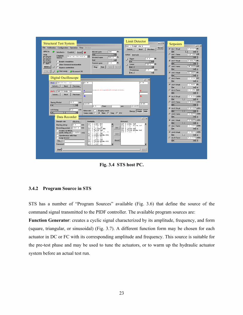
23
Structural Test System Limit DetectorSetpoints
Digital Oscilloscope
Data Recorder
Structural Test System Limit DetectorSetpoints
Digital Oscilloscope
Data Recorder
Fig. 3.4 STS host PC.
3.4.2 Program Source in STS
STS has a number of “Program Sources” available (Fig. 3.6) that define the source of the
command signal transmitted to the PIDF controller. The available program sources are:
Function Generator: creates a cyclic signal characterized by its amplitude, frequency, and form
(square, triangular, or sinusoidal) (Fig. 3.7). A different function form may be chosen for each
actuator in DC or FC with its corresponding amplitude and frequency. This source is suitable for
the pre-test phase and may be used to tune the actuators, or to warm up the hydraulic actuator
system before an actual test run.

24
(a) DC (b) FC
Fig. 3.5 PIDF controls of displacement (DC) and force (FC) in STS.
Fig. 3.6 Available program sources in STS.
Data Player File: used for applying a previously recorded load sequence.
Remote Application: provides the possibility of sending target commands from an outer source
through Ethernet connection.
ScramNet: transmits the command signals from xPC target, discussed in the next section, to STS
in real time where STS updates its memory at 1024 Hz. This source is used for the present HS.
Discussion on ScramNet has been previously presented in Section 3.3.
Pod: allows the actuators to be controlled manually through a mobile pod available on the
structural laboratory, which gives the user control over the actuator(s) to a high degree of
accuracy (within thousandths of an inch), while observing the test structure and actuator. This is
mainly used for the attachment of the actuator to the test structure.

25
Fig. 3.7 Function generator in STS.
3.5 xPC TARGET
xPC target is a solution for prototyping, testing, and deploying real-time systems using standard
PC hardware. It is an environment that uses a target PC, separate from a host PC, for running
real-time applications. In the present study, xPC target is used as a link, running compiled
Simulink models and operating in real time, between the STS controller and the MATLAB
environment, discussed in Section 3.7. It is programmed on the host PC using MATLAB,
Simulink, and Stateflow. The information exchanged between the two entities, namely STS
controller and the MATLAB environment, includes feedback signals and control modes. In
Figure 3.8, the left block represents the input parameters transmitted from STS to xPC, while the
right block represents the output parameters sent from xPC to STS. The middle block is the mask
for the operations performed by xPC using the input signals to produce the output signals and is
expanded in Figure 3.9. The upper and lower lines, on the left hand side of the figure, are the
displacement feedback and force feedback signals, respectively, of the eight actuators that may
be incorporated in the model. Two actuators are used in this case and a series of operations is
performed including the exchange of information with the MATLAB environment. The set of
output (displacement command) signals is assembled at the vertical line, on the right-hand side
of the figure, and passed to the STS controller through ScramNet.

26
Fig. 3.8 Simulink model for xPC target.
Once the MATLAB environment computes the required information such as command
values at the end of each integration time step as well as control modes, i.e., displacement or
force in mixed-variables control discussed in Chapter 6, this information is transmitted to the
xPC target. These signals are transformed into real-time interrupts (1024 Hz) in the Simulink
model, which is linked to the STS controller in real time through ScramNet. The transformation
is performed through a process of extrapolation/interpolation, as described in Section 3.8, where
a variety of extrapolation and interpolation protocols are available. One of these protocols,
namely the third-degree Lagrange polynomial (Mosqueda 2003), is used in the present study.
This protocol ensures that the velocity of the actuator, dictated by the predicted target for
extrapolation, closely matches the velocity implied by the calculated target displacement from an
explicit integration algorithm in the same time step, thus causing the least disturbance possible to
the motion of the actuators. This protocol, however, is not suitable for an implicit integration
algorithm, where the iterations within the same integration time step do not necessarily follow
the expected velocity pattern and where the displacement increments in one iteration may be in
the opposite direction to the previous ones (same for velocities). In this case, and to avoid
unrealistic loading/unloading cycles that may be caused by an erroneous predicted target for
extrapolation, a linear interpolation from the current state to the new command is preferred. At

27
the end of the time step, as soon as the desired command is executed by the PIDF controller, the
feedback signals corresponding to the implemented command are transferred to the MATLAB
environment. Finally, xPC target offers an environment where the real-time data are available for
special procedures such as computations related to the estimation of the secant stiffness, as
discussed in Chapter 6.
Fig. 3.9 Expansion of operation block in Simulink model for xPC target.
3.6 PACIFIC INSTRUMENTS DATA-ACQUISITION SYSTEM
The Pacific Instruments data-acquisition system is a receiver and compiler of all the information
available from the instruments installed on the test structure. The software that runs the hardware
interface on the host computer for the purpose of data acquisition is PI660 (Pacific Instruments
2004). The system has a capacity of 128 channels at a maximum sampling rate of 50 kHz.
Sixteen additional channels are provided for STS feedback signals. High-pass filters, at the
desired cut-off frequency, are provided for all channels. The acquired information is stored on
the Pacific Instruments host PC for extraction after the completion of the test and is available on

28
ScramNet during the online experiment in real time for possible use within the online
calculations.
The calibration process of all the instruments is performed through the interactive
interface provided by the Pacific Instruments software (Fig. 3.10). Each horizontal line (row)
represents a channel and its information is displayed in the respective columns, such as the type
of instrument, the engineering unit used and the status, to indicate the completion of the
calibration process, of voltage (V), and engineering unit (EU) calibrations that relate V output
signals to measured quantities in EU. The system also provides a number of real-time viewing
options including oscilloscopes and tables in engineering units.
Fig. 3.10 Calibration of sensors in Pacific Instruments data-acquisition system.
3.7 MATLAB ENVIRONMENT
MATLAB is used in the test setup for the present study as the main site for the HS calculations.
An Ethernet connection links the PC operating MATLAB to the xPC target. Therefore,
MATLAB has access to the STS controller feedback information available through xPC target,
as well as the Pacific Instruments data-acquisition information through ScramNet (Fig. 3.2). The

29
HS numerical-integration algorithm is programmed in the MATLAB environment together with
numerical substructuring computations and the live displays for monitoring while online
experiments are in progress.
It is worthy to note that MATLAB is not the only environment available in the HSS to
run and control xPC target applications. A similar connection may be established with a C/C++
environment through the xPC target application program interface where other programs such as
OpenSees (Open source for earthquake engineering simulation) (Mazzoni et al. 2006) may be
used to replace MATLAB (Fenves et al. 2004; Schellenberg et al. 2007).
3.8 OPERATION SEQUENCE IN HSS
The operation sequence during the i -th numerical-integration time step with time-step duration
dt is discussed. Based on a prediction/correction scheme, using polynomial
extrapolation/interpolation, designed to keep the actuators in continuous motions (Nakashima
and Masaoka 1999; Mosqueda 2003), the sequence in Figure 3.11 is as follows: • 1−iD marks the end of execution, by the hydraulic system, of the command signal from
the previous time-step number 1−i . At this point, xPC target starts an extrapolation
process of the command signals and continues communicating with STS by sending and
receiving command and feedback signals, respectively. • At iA , a new integration time step begins where MATLAB receives the feedback from
the previous time step through xPC target. This feedback is the latest received by xPC
from STS and is used by MATLAB to calculate the next command signal. • Between iA and iB , MATLAB performs its calculations and xPC continues
extrapolating commands to send to STS keeping the actuators in continuous motions. • At iB , MATLAB is ready with the command signals for step number i , which are
subsequently sent to xPC target. • At iC , xPC receives the target commands and immediately stops extrapolating and starts
interpolating toward the current commands. Concurrently, MATLAB performs other
tasks, e.g., calculations related to substructuring or data displays.

30
• At iD , the actuators reach the commands of time step i ending interpolation and starting
extrapolation in xPC target for the next time step 1+i and then repeating the above
sequence. • Throughout the online experiment, xPC target is constantly sending command values to
STS at time intervals 10241=tδ sec, whether deduced by extrapolation or by
interpolation, and receiving feedbacks. Provided that the time needed to reach iC from
1−iD is small compared with dt , each time step is performed in the prescribed dt .
However, in case of a delay in one or more of the steps in the previously discussed
operation, the hydraulic system goes into a “slow” mode, i.e., slower than the prescribed
dt to reach the target command signals, followed by a system “hold” mode if needed for
long delays, causing the experiment to run slower than desired (Mosqueda 2003).
MatLab & xPC host
xPC target
STS
Integration algorithm
Substructure computations
Interpolation
PIDF controlA/D conversionD/A conversion
+ Displays
Extrapolation
DAQ Data acquisition system
time
Extrapo. …
Integ. …
Ai Bi Ci Di Ai+1
Hydraulic system + Actuators + Specimens
dt
δt
δt
DAQδt
Di-1
MatLab & xPC host
xPC target
STS
Integration algorithm
Substructure computations
Interpolation
PIDF controlA/D conversionD/A conversion
+ Displays
Extrapolation
DAQ Data acquisition system
time
Extrapo. …
Integ. …
Ai Bi Ci Di Ai+1
Hydraulic system + Actuators + Specimens
dt
δt
δt
DAQδt
Di-1
Fig. 3.11 Operation sequence in HS.

31
The data-acquisition is operating in parallel to the previously discussed sequence. In this
operation, data are extracted from the instruments installed directly on the test structure or in the
attached actuators at the selected sampling rate with time interval DAQtδ , not necessarily the same
as tδ . However, this data-acquisition system information is readily available online for all
components of the HSS through ScramNet.
3.9 VALIDATION OF HSS
To evaluate the performance of the HSS, an online (pseudo-dynamic) experiment is designed
with a numerically reproducible structural behavior of the test structure where test results can be
validated against pure numerical simulation. Two steel cantilever columns, 1C and 2C , constitute
the two physical substructures and are installed on the strong floor and connected to the same
actuators used in the experimental program of the present study (Fig. 3.12(a)). Column 1C is
designed to behave linearly and is tested in its elastic range. Column 2C is the same as 1C but is
stiffened by a shorter cantilever adjacent to it when an adjustable initial gap closes in the push or
pull loading directions. The design details are shown in Figure 3.12(b). Accordingly, the
validation test structure is a coupled two-DOF system (Fig. 3.13) with linear and stiffening
bilinear behaviors for 1C and 2C , respectively (Fig. 3.14), with a fundamental natural period of
0.31 sec. The structural parameters used for the online HS of the two columns are summarized in
Table 3.2. A numerically simulated linear spring with high stiffness ( lk ) connects the two DOF
of 1C and 2C in parallel, thus forcing them to be fully coupled, i.e., subjecting them to similar
displacement time history.
Although the linear spring is of high stiffness ( lk ), the difference in the displacement
between the two DOF is not to be entirely neglected and was a subject of study in itself. That is,
the HS validation system is intended to mimic the system of test structure A in phase S-1 (see
Fig. 1.2), where the RC bare frame is expected to be relatively flexible when compared to the
URM infilled one, Chapter 4. An RC slab connects the RC frames and is analogous to the linear
high-stiffness numerical spring ( lk ) used in the validation experiment. Moreover, the same
numerical-integration algorithm implemented for the simulation of test structure A is used in the
present validation experiment. The experiment therefore, not only serves to validate the HSS, but

32
also serves as a trial run on a system similar to that in phase S-1 for test structure A (see Fig.
1.2), and inspects the potential problems that may arise during the HS experiment of test
structure A, whether in the numerical-integration algorithm or in the simulation of a two-DOF
system exhibiting stiff and flexible behaviors.
C1
2C
(a) Setup of steel specimens in structural laboratory
Dimensions in mm
[1"=25.4 mm ]
Dimensions in mm
[1"=25.4 mm ]
(b) Cantilever 2C with bilinear behavior ( 1C is similar but without cantilever stiffener)
Fig. 3.12 Steel specimens design and setup in structural laboratory.

33
Table 3.2 Evaluated parameters for validation of HSS.
Parameter Value Linear stiffness,
1Ck [kip/in. (kN/mm)] 0.613 (3.50)
Initial stiffness, ICk
2 [kip/in. (kN/mm)] 0.536 (3.06)
Secondary stiffness, SCk
2 [kip/in. (kN/mm)] 2.011 (11.48)
Connecting stiffness, lk [kip/in. (kN/mm)] 1650 (289.0)
Stiffness ratio, IC
SC kk
22 3.75
Mass for 1C (1Cm ) [kip-sec2/in. (kN-sec2/mm)] 0.0017 (0.0096)
Mass for 2C (2Cm ) [kip-sec2/in. (kN-
sec2/mm)] 0.0011 (0.0061)
Damping ratio (%) 5 Numerical-integration time step (sec) 0.01
Physical substructures
1Cm
1Ck2Ck
2Cmlk
Physical substructures
1Cm
1Ck2Ck
2Cmlk
Fig. 3.13 Idealized model for HS validation structure.
The two DOF validation test structure is excited by the strong motion, Northridge,
Tarzana station, 1994 earthquake scaled to 17% of the original record described in Table 4.1.
Using the evaluated stiffness of the columns from the test results (Fig. 3.14), pure numerical
simulation validates the experimental results with good accuracy, as illustrated in Figure 3.15,
where representative numerical samples are shown along the displacement time history with a
maximum error of 6.8%, relative to the peak recorded displacement.

34
Displacement [mm]-30.4 -15.2 0 15.2 30.4
Displacement [mm]-30.4 -15.2 0 15.2 30.4
Forc
e [k
N]
35.6
17.8
0
-17.8
-35.6-1.2 -0.6 0 0.6 1.2-8
-4
0
4
8
Displacement [in]
Forc
e [k
ip]
Linear
-1.2 -0.6 0 0.6 1.2-8
-4
0
4
8
Displacement [in]
Bilinear
Displacement [mm]-30.4 -15.2 0 15.2 30.4
Displacement [mm]-30.4 -15.2 0 15.2 30.4
Forc
e [k
N]
35.6
17.8
0
-17.8
-35.6-1.2 -0.6 0 0.6 1.2-8
-4
0
4
8
Displacement [in]
Forc
e [k
ip]
Linear
-1.2 -0.6 0 0.6 1.2-8
-4
0
4
8
Displacement [in]
Bilinear
Fig. 3.14 Structural response of physical substructures 1C (left) and 2C (right).
Dis
plac
emen
t [m
m]
Dis
plac
emen
t [m
m]
30.4
15.2
0
-15.2
-30.4
30.4
15.2
0
-15.2
-30.4
0 5 10 15 20-1.2
-0.6
0
0.6
1.2
Time [sec]
Disp
lace
men
t [in
]
0.37
1.03
-0.46 -0.64
0.28
HS results
0 5 10 15 20-1.2
-0.6
0
0.6
1.2
Time [sec]
Disp
lace
men
t [in
]
0.37
1.02
-0.48 -0.68
0.3
Pure NS results
Dis
plac
emen
t [m
m]
Dis
plac
emen
t [m
m]
30.4
15.2
0
-15.2
-30.4
30.4
15.2
0
-15.2
-30.4
0 5 10 15 20-1.2
-0.6
0
0.6
1.2
Time [sec]
Disp
lace
men
t [in
]
0.37
1.03
-0.46 -0.64
0.28
HS results
0 5 10 15 20-1.2
-0.6
0
0.6
1.2
Time [sec]
Disp
lace
men
t [in
]
0.37
1.02
-0.48 -0.68
0.3
Pure NS results
Fig. 3.15 Validation of HSS.

35
3.10 SUMMARY
The hybrid simulation system developed as part of nees@berkeley at the University of
California, Berkeley, is presented. The components of the hybrid simulation system used in the
present study are identified and described each in terms of its function and interconnection with
the other components. The operation sequence of the hybrid simulation system during one
numerical-integration time step of a generic online experiment is presented. Finally, a steel
cantilever test structure is physically tested in a hybrid simulation setting and the results are
validated against a pure numerical simulation. From this validation exercise, functionality of the
newly installed hybrid simulation system is judged to be accurate and reliable.

4 Test Structure A
The first test structure presented in this chapter consists of two large substructures of an ST
experiment conducted at UCB. The ST test structure is briefly presented along with the selection
of the strong motions applied during different phases of the experiment. This chapter describes
the physical substructures including design, construction, and instrumentation. In addition, the
test setup is discussed in terms of its design and assembly as a means of demonstrating the
functionality of nees@berkeley. Moreover, the development of the computational part of the HS
for this test structure is discussed. This includes the idealization of the test structure, the
formulation of the governing equations of motion, and the estimation of some key parameters in
these equations.
4.1 ST TEST STRUCTURE
A hypothetical five-story prototype structure with RC frames and URM infill walls is considered.
The URM infill walls are assumed in the interior frames (Fig. 4.l(a)). The ST experiment is
carried out on a reduced-scale one-story RC moment-resisting frame structure with URM infill
wall on the seismic simulator test facility of UCB. The three-fourths-scale test structure
represents the first-story middle bays of the prototype structure. The structure is designed based
on the requirements of ACI318-02 (2002) and NEHRP recommendations (BSSC 2000) in
seismic regions (Fig. 4.1(b)). As in the prototype structure, the URM infill wall of the ST test
structure is constructed in the interior frame only. Moreover, a computationally determined
additional mass is placed on the RC slab of the ST test structure with the objective of matching
the base shear of this test structure with that of the prototype building when subjected to the
design-level ground motion (Hashemi and Mosalam 2006, 2007). This additional mass and the
mass of the ST test structure itself represent the total mass considered numerically in the HS
experiments corresponding to the ST experiments. To simulate the effect of the upper stories of

38
the prototype building on the RC columns of the tested first-story structure, post-tensioning
through concentric rods in all columns is included in the structures tested on the ST and using
HS. Three test phases are performed as outlined in Figure 1.2. These three phases are reproduced
on an identical test structure in the HS experiments. Therefore, the ST experiment serves as a
benchmark for the HS experimental approach.
A3A0 A2A1
B0 B1 B3B2
C2 C3
5 @
108
" (2
740
mm
)
C1
(a) Hypothetical five-story prototype
structure (b) One-story ST test structure
Fig. 4.1 Five-story prototype and one-story ST structures (Hashemi and Mosalam 2007).
4.2 STRONG MOTION SELECTION
In the test phases of structure evaluation, denoted by “S” in Figure 1.2, to compare with the
parallel ST tests, the same strong motions as those used in the ST tests are adopted in the HS.
Table 4.1 describes the strong motions selected for test structure A where PGA, PGV, and PGD
refer to peak ground acceleration, velocity, and displacement, respectively. These ground
motions are intended to be unidirectional in the direction parallel to the URM infill wall of the
test structure (longitudinal direction).
Table 4.1 Ground motion specifications (1 in. = 25.4 mm).
Ground Motion Station Direction PGA (g) PGV (in./sec) PGD (in.)
Northridge, CA, 1994 (TAR) Tarzana 090 1.570 36.23 5.13 Düzce, Turkey, 1999 (DUZ) Lamont N 0.762 12.97 0.75
Loma Prieta, CA, 1989 (LPB) Bran 000 0.426 17.43 2.28

39
Figure 4.1 shows the 5% damping acceleration response spectra for the three strong
motions together with the NEHRP design spectrum. Each ground motion is scaled to generate
different levels of intensity as listed in Table 4.2. The scaling is based on the average spectral
acceleration of the selected ground motions over the range that the period of the test structure is
expected to vary during the experiments, and the NEHRP design spectrum for a site with mapped
spectral response acceleration at 1 sec, gS 65.01 = , and at short periods, gSs 60.1= , and site
class D with 5% damping. Level 1 is selected as a very small amplitude motion to check the
performance of the data-acquisition system. Levels 2 and 3 are selected as low-intensity level
motions while level 4 corresponds to the design level spectrum and level 6 corresponds to the
maximum considered earthquake spectrum. Levels 7 and up are selected to achieve higher
demands on the test structure considering the limits of the ST. The ground motion records are
also compressed in time by a factor of 43 to account for the 43 length scale of the test
structure. In this way the frequency content of the record at the natural period of the undamaged
test structure is the same as the prototype first-story substructure, i.e., without scaling.
0 0.5 1 1.5 20
0.2
0.4
0.6
0.8
1
1.2
1.4
1.6
1.8
2
Period [sec]
Spec
tral a
ccel
erat
ion
[g]
TARDUZLPBDesign 0 5 10 15 20 25
-101
Northridge, Tarzana
0 5 10 15 20 25-101
Acc
eler
atio
n [g
] Duzce
0 5 10 15 20 25-101
time [sec]
Loma Prieta, Bran
0 0.5 1 1.5 20
0.2
0.4
0.6
0.8
1
1.2
1.4
1.6
1.8
2
Period [sec]
Spec
tral a
ccel
erat
ion
[g]
TARDUZLPBDesign 0 5 10 15 20 25
-101
Northridge, Tarzana
0 5 10 15 20 25-101
Acc
eler
atio
n [g
] Duzce
0 5 10 15 20 25-101
time [sec]
Loma Prieta, Bran
Fig. 4.2 Response spectra with 5% damping for selected ground motions (Hashemi and Mosalam 2007).

40
Table 4.2 Scale factors for different levels of input ground motions.
Level 1 2 3 4 6 7 8 9 10 Northridge, CA, 1994 (TAR) 0.05 0.17 0.23 0.39 0.59 - - - - Düzce, Turkey, 1999 (DUZ) - - - - - 1.50 2.00 2.53 -
Loma Prieta, CA, 1989 (LPB) - 0.31 0.44 0.67 1.00 1.50 1.95 2.19 3.29
Since the ST is not capable of exactly reproducing the input strong motions, the
accelerations are measured on the table during each ST run and this measured (output) response
of the table is applied in the HS rather than the original scaled input motion to the table.
Moreover, the recorded acceleration time histories included high-frequency content (>25 Hz),
introduced mainly by the electrical noise in the connecting cables when recording the output
signals. Since these frequencies are too high to have any structural significance during the
dynamic experiment on the test structure, a low-pass filter is applied to eliminate these high
frequencies, while preserving the recorded lower frequencies (Fig. 4.3).
The diagram in Figure 4.4 illustrates the chronological order of the strong motions
applied in each of the three structural evaluation phases of test structure A. Note that each event
is labeled by the name of the strong motion, e.g., TAR in Table 4.1, followed by the intensity
level, e.g., 2 in Table 4.2. The last two digits if present designate the repetition number of that
level and the phase number between brackets, respectively. These two numbers are omitted if
their value is one, e.g., TAR-4-2[2] designates the second repetition of TAR strong motion at
intensity level 4 in phase 2 of the experiments, while TAR-2 designates the first run of TAR at
intensity level 2 in phase 1 of the experiments.

41
0 5 10 15 20 25 30-0.4
-0.2
0
0.2
0.4
Time [sec]
Acc
eler
atio
n [g
]
(a) ST output time history
0 5 10 15 20 25 30-0.4
-0.2
0
0.2
0.4
Time [sec]
Acc
eler
atio
n [g
]
(b) Filtered signal time history
7.8 8 8.2 8.4 8.6 8.80
0.05
0.1
0.15
0.2
Time [sec]
Acc
eler
atio
n [g
] FilteredTable
(c) Zoomed in part of time histories
Fig. 4.3 Filtering of acceleration time history of ST output signal for TAR level 2.

42
TAR
-1
TAR
-2
TAR
-3
TAR
-4
TAR
-6
DU
Z-7
DU
Z-8
DU
Z-9
DU
Z-9-
2
TAR
-1[2
]
TAR
-2[2
]
TAR
-4[2
]
TAR
-4-2
[2]
TAR
-4-3
[2]
DU
Z-9[
2]
LPB
-2[2
]
LPB
-7[2
]
LPB
-9[2
]
LPB
-9-2
[2]
LPB
-2[3
]
LPB
-2-2
[3]
LPB
-7[3
]
LPB
-8[3
]
LPB
-9[3
]
LPB
-9-2
[3]
LPB
-9-7
[3]
LPB
-10[
3]
Phase S-1
Phase S-2
Phase S-3
. . .
TAR
-1
TAR
-2
TAR
-3
TAR
-4
TAR
-6
DU
Z-7
DU
Z-8
DU
Z-9
DU
Z-9-
2
TAR
-1[2
]
TAR
-2[2
]
TAR
-4[2
]
TAR
-4-2
[2]
TAR
-4-3
[2]
DU
Z-9[
2]
LPB
-2[2
]
LPB
-7[2
]
LPB
-9[2
]
LPB
-9-2
[2]
LPB
-2[3
]
LPB
-2-2
[3]
LPB
-7[3
]
LPB
-8[3
]
LPB
-9[3
]
LPB
-9-2
[3]
LPB
-9-7
[3]
LPB
-10[
3]
Phase S-1
Phase S-2
Phase S-3
. . .
Fig. 4.4 Chronological order of events for test structure A.
4.3 PHYSICAL SUBSTRUCTURES IN HS
Each test structure in the outlined phases of the HS experimental program (Fig. 1.2) consists of
physically tested substructure(s) using the hydraulic system and a numerically simulated
substructure. The physical substructures used in all experiments are two ¾-scale RC frames with
fixed footings to the strong floor of the structural laboratory. The first frame is infilled using
URM wall, this is denoted F1I (frame no. 1 infilled). The second frame is not infilled and is
denoted F2B (frame no. 2 bare). After the collapse of the URM infill wall, F1I is used for further
testing after the complete removal of the collapsed URM infill wall and in this form is denoted
F1B (frame no. 1 bare). Note that the URM infill wall protected the members of the bounding
RC frame as discussed in subsequent chapters. This allowed the reuse of the RC frame of F1I as
F1B after removal of the URM infill wall. All columns of the test frames are post-tensioned
using concentric high-strength steel rods to account for the effect of the upper stories of a
prototype building (Hashemi and Mosalam 2006). In later phases of testing, some of the
experiments are conducted without the post-tensioning. The RC frames are then denoted F1BU
and F2BU (frames no. 1 and 2 bare without post-tensioning). Table 4.3 summarizes the different
states of the tested frames.

43
Table 4.3 Physical substructures in HS.
Frame Notation Description
F1I RC frame No. 1, infilled using URM wall F1B RC frame No. 1, after collapse and removal of the URM infill wall F2B RC frame No. 2, no infill is present, i.e., bare
F1BU RC frame No. 1, same as F1B after removal of the column post-tensioning F2BU RC frame No. 2, the column post-tensioning of F2B is removed
The test structures used in the experiments are categorized as follows, based on the intended
purpose of the experiments for the different phases as shown in Figure 1.2: • Test structure in S-1: Three one-bay RC frames are connected with a RC slab at the level
of the top beams (Fig. 4.5(a)). The URM infill wall is constructed inside the middle frame
without any additional connection to the surrounding frame other than cement mortar.
Frames F1I and F2B represent the physical substructures; the response of the remaining
outer frame (identical to F2B because of symmetry) and the connecting RC slab are
numerically modeled. The modeling details are discussed in subsequent sections. • Test structure in S-2: This phase follows heavy damage of the URM infill wall and its
removal. The test structure is the same as the one in S-1, with the exception that the URM
infill wall is absent. Only frame F2B is used as the physical substructure, while the
remaining two bare frames (identical to F2B from the stiffness point of view) and the
connecting RC slab are numerically modeled. Note that the mass is not distributed evenly
over the three RC frames as discussed in Section 4.10.1 and shown in Figure 4.23. • Test structure in S-3: The test structure is the same as the one in S-2, with the exception
that the column post-tensioning is removed. Frame F1BU or F2BU is used as the physical
substructure interchangeably (one of these two frames is used at a time to study the effect
of different parameters in the developed HS), while the remaining two bare frames and
the connecting RC slab are numerically modeled. • Test structure in P-1 and P-2: The test structure is the same as the one in S-2, except that
F1B is used instead of F2B.

44
F1I F2BF1I F2B
F2BF2B
(a) Test structure in S-1 (b) Test structure in S-2
Fig. 4.5 Test structures in HS.
4.4 RC FRAME DESIGN
To compare the HS results to its parallel counterpart on the ST, the design of the RC frames
tested on the ST (Hashemi and Mosalam 2006, 2007) is adopted in this study (see Fig. 4.6). The
center-to-center span of each frame is 13'-6" (4.11 m) with a total height of 10'-9" (3.28 m).
Column sections are 12"×12" (305 mm×305 mm) with 8 #6 (19 mm diameter) longitudinal
reinforcing bars and an unbonded 1¼" diameter (32 mm) post-tensioning central rod to represent
column axial loads from the not modeled upper stories of the prototype building. The transverse
reinforcing bars of the columns consist of #3@3¾" (10 mm diameter@95 mm) over 24" (610
mm) from the face of the column-to-footing and beam-to-column joints and #3@6" (10 mm
diameter@152 mm) elsewhere. Long-direction single-span beam sections are 10½"×13½" (267
mm×343 mm) with 3#6 (19 mm diameter) top and bottom longitudinal reinforcing bars. Beam
transverse reinforcing bars are #3@2¾" (10 mm diameter@70 mm) over 28" (711 mm) from the
face of the beam-to-column joint and #3@8" (10 mm diameter@203 mm) elsewhere. Design
details are illustrated in Figure 4.7, and more information on the prototype structure is
documented in Hashemi and Mosalam (2006). While the ST test structure consists of RC frames
connected using a 3¾" (95 mm) thick RC slab with #3 (10 mm diameter) reinforcing bars top
and bottom at 12" (305 mm) on center each way, the HS test structure consists of two separately
constructed frames and the RC slab is numerically simulated, as discussed in the following
chapters. However, in addition to the role of the RC slab in connecting the frames, it contributes
to the beam structural strength and stiffness with an effective slab width. This effective width is
estimated to be 20.25" (514 mm) from the center of the beam to each side according to ACI318-
02 Section 8.10.2 (total effective width ≈ 40.5" (1029 mm)). However, in the ST experiment
(Hashemi and Mosalam 2007), this width was estimated to be on the order of 10" (254 mm) on

45
each side of the beam center line (total effective width ≈ 20" (508 mm)). A total effective RC
slab width of 28.5" (724 mm) is adopted in the HS test structure, which falls between the
American Concrete Institute (ACI) and the experimental estimates, and the slab is constructed
integrally with the RC beam. The URM infill wall is made of clay bricks with modular size of
4"×8"×2⅔" (102 mm×203 mm×68 mm) and ASTM C270 (2003) Type N mortar. The infill wall
is constructed over a RC grade beam as shown in Figure 4.6. Design details including beam,
column, and foundation cross sections, and concentric post-tensioning rods of the column, are
shown in Figure 4.7.
1'-2
"
3" DIA. HOLE PROVIDED FOR ATTACHMENT TO THE STRONG FLOOR
13'-6"
2
6"
1
LC
1'-1
.5"
CLAY BRICKS, MODULAR SIZE:
4x8x223 W/ 38"
MORTAR JOINT TYPE N.
2'-3"
#3@4" O.C.
11-#3@234"
O.C. STIRRUPS
10-#
3@33 4"
O.C
. HO
OPS
#3@6" O.C.
10-#
3@33 4"
O.C
. HO
OPS
#3@8" O.C.
3-#6 TOP
3-#6 BOT.
8-#6 COLUMN LONG. REINF.
GRADE BEAM
4-#7 BOT.
4-#7 TOP
6"
7'-0" 5'-0"
19'-0"
CONCENTRICPVC TUBE TO ACCOMODATE POST-TENIOSIONINGHIGH-STRENGTHROD
Fig. 4.6 Infilled frame reinforcement (bare frame is similar without URM infill wall and grade beam) (1'=304.8 mm, 1"=25.4 mm).

46
312"Ø PVC TUBE
4-#7 BOT.
8"x8"x112" STEEL
PLATE
2"Ø PVC TUBE
1'-1
.50"
LONG.
10"SLAB REINF.
#3 STIRRUPS
2'-4.5"3.75
"
SLAB REINF.
REINFORCEMENT
334" THK CONCRETE
SLAB W/#3@12" T&B EA. WAY
BEAM - SLAB DETAIL
10.5"3 #6 LONG.
3-#6 TOP
BEAM-COLUMN JOINT
INTO THE JOINTHOOPS CONTINUE COLUMN
#6 BEAM23
4"
#6 COLUMN LONG.
6.0"
1'-1
.5"
10"
9"33 4"
#3 HOOPS
#3 STIRRUPS
2-#3STIRRUPS
34" CLEAR COVERON ALL SIDES
1'-0"
COLUMN SECTION
1'-0
"
#3 HOOPS
REINFORCEMENT8-#6 LONG.
34" CLEAR COVERON ALL SIDES
TOPREINFORCEMENT
#3 STIRRUPS @4"
4-#7 LONG.
1'-2
"
FOUNDATION SECTION4-#7 BOT.
1'-6"6"
TOP PLATE
0.375"Ø
1.65"
8"8"
1.5"
114"Ø HOLE
2"Ø PVC TUBE
8"x8"x112"
Steel PlateHEX NUT
1"Ø GRADE 150 PARTIALLY THREADED BARLENGTH = 139"
60° HOLE PROVIDED FOR STRAIN GAGE WIRES
1"Ø GRADE 150 PARTIALLY THREADED BARLENGTH = 139"
1'-2
" 8"1.5"
3.5"Ø
~3"
BOTTOM PLATE
Fig. 4.7 Design details of RC frames (1'=304.8 mm, 1"=25.4 mm).
4.5 INSTRUMENTATION
The two RC frames of the test structures are identically instrumented. Strain gages are installed
on the reinforcing steel bars in the beams and columns. Starting from the beam-to-column and
the column-to-footing joints, the strain gages are positioned at six cross sections in the beam and
six cross sections in the columns at increasing distances from these joints (Fig. 4.8). Each cross
section contains three strain gages, two on the middle bars of the longitudinal steel, and the third
on a transverse reinforcing bar. A total of 54 strain gages are employed per frame (Fig. 4.8).

47
56
49
125
106 126
105 115
4 104 10
93 103
102 82
101 71
5758
50
126
51
127
60
59
53
128
6162
5455
130
11218 24
1
129
52
2317 111
2216 110
2115 109
20
19
14
13 107
108
2Instrumentedbars in beams
Instrumentedbars in columns
Fig. 4.8 Strain gages numbering on reinforcing steel bars in RC frames.
External instrumentation consists of displacement transducers in the columns along the
height of each column (Fig. 4.9). Additional 14 transducers are used for the URM infill wall to
measure diagonal deformations as well as relative movement (opening and sliding) between the
infill wall and the bounding frame. In addition, one accelerometer is installed on top of each
frame to measure in-plane accelerations in the case of fast rate loading. As an example, the
ground motion LPB-9 (Tables 4.1–4.2) is conducted 20 times slower than real time. The ratio of
the measured acceleration, on the physical substructure F1B, is theoretically 102 = 100 times less
than the numerically simulated one as is confirmed by the plotted acceleration time histories in
Figure 4.10.

48
(a) Layout and numbering of displacement transducers
(b) Photograph of instrumented URM infilled frame
Fig. 4.9 Numbered displacement transducers on URM infilled RC frame.

49
0 2 4 6 8 10 12 14 16-0.01
-0.005
0
0.005
0.01
Time [sec]
Acc
eler
atio
n [g
]
(a) Measured acceleration on physical substructure F1B
0 2 4 6 8 10 12 14 16-1.5
-1
-0.5
0
0.5
1
1.5
Time [sec]
Acc
eler
atio
n [g
]
(b) Numerically simulated acceleration
Fig. 4.10 Accelerations at faster rate execution, LPB-9 at 20 times slower than real time.
Two wire potentiometers per frame, labeled 1 to 4 in Figure 4.16(a), measure the out-of-
plane displacements at the centerline of each column. The maximum out-of-plane drift, defined
with respect to the frame height, i.e., 110 in. (2794 mm), in the case where the structure in phase
S-1 (see Fig. 1.2) is subjected to the strong motion TAR-6 (Tables 4.1–4.2) and is evaluated to
be 0.3% for F2B (Fig. 4.11). These recorded out-of-plane drifts are considered not large enough
to require any out-of-plane restraint for the test structure such that the pure in-plane loading
nature of the test is practically preserved.
0 10 20-0.5
-0.25
0
0.25
0.5
Time [sec]
Out
of p
lane
drif
t [%
]
Out-of-plane 1Out-of-plane 2
Fig. 4.11 Out-of-plane drift measurements in TAR-6 frame F2B, phase S-1.
50
4.6 CONSTRUCTION AND MATERIAL PROPERTIES
The RC frames are constructed using professional contractors. The strain gages are installed on
the reinforcing steel bars and covered with adequate protection layers to ensure their continuous
functionality after the concrete is cast (Fig. 4.12(a)). The concrete is placed on three lifts
(foundations, columns, and beams) to simulate the typical construction joints in real conditions
(Fig. 4.12). Concrete cylinders are cast from the same concrete mix and tested at progressing
ages. Table 4.4 and Figure 4.13 show the values of the estimated compressive strength from the
average of three 6"×12" standard cylinders (ASTM C837-99) at different ages and locations.
After the RC frames are placed in their setup positions on the strong floor, the URM infill wall is
constructed in place by professional masons. Masonry prisms (4"×8"×12") are constructed for
the purpose of determining the uniaxial compressive strength of masonry. The average
compressive strength of three prisms tested at 28 days is 2087 psi (14.4 N/mm2), with failure
characterized by double face shell crushing mode (ASTM C1314-02a).
4.7 EXPERIMENTAL SETUP DESIGN
The RRW of the structural laboratory as part of nees@berkeley offers flexibility in the layout of
the test setup. This section describes the steps in the design of the experimental setup for the
purpose of the present study.
4.7.1 Reaction Wall Design and Actuator Selection
For each experimental substructure, one reaction wall and one actuator are utilized. Table 4.5
summarizes the main properties of the two substructures, based on which the proper actuators are
selected and the reaction wall heights and locations on the strong floor are determined. The
expected maximum applied loads in Table 4.5 are based on the performance of the ST test
structure (Hashemi and Mosalam 2007). The displacement limits are related to the expected
largest lateral drift. Note that the ±8 in. (±203 mm) limit corresponds to ±7.3% lateral drift of the
one-story RC frames of test structure A.

51
(a) Strain gage on reinforcing steel bar (b) Overview of forms and column cages
(c) Placement of concrete in foundation (d) Top view of concentric post-
tensioning rod
(e) Steel reinforcement in beam and slab (f) Construction of URM infill wall
Fig. 4.12 Construction of RC frames.
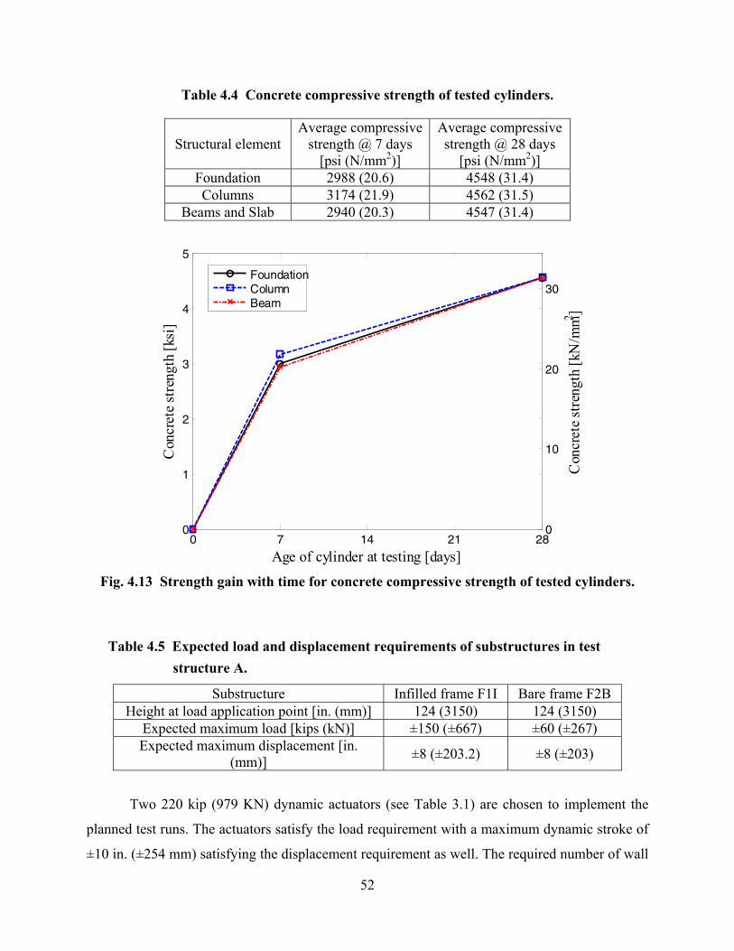
52
Table 4.4 Concrete compressive strength of tested cylinders.
Structural element Average compressive
strength @ 7 days [psi (N/mm2)]
Average compressive strength @ 28 days
[psi (N/mm2)] Foundation 2988 (20.6) 4548 (31.4) Columns 3174 (21.9) 4562 (31.5)
Beams and Slab 2940 (20.3) 4547 (31.4)
0 7 14 21 280
1
2
3
4
5
Con
cret
e stre
ngth
[ksi
]
Age of cylinder at testing [days]
0
10
20
30
Con
cret
e stre
ngth
[kN
/mm2 ]
FoundationColumnBeam
Fig. 4.13 Strength gain with time for concrete compressive strength of tested cylinders.
Table 4.5 Expected load and displacement requirements of substructures in test structure A.
Substructure Infilled frame F1I Bare frame F2B Height at load application point [in. (mm)] 124 (3150) 124 (3150)
Expected maximum load [kips (kN)] ±150 (±667) ±60 (±267) Expected maximum displacement [in.
(mm)] ±8 (±203.2) ±8 (±203)
Two 220 kip (979 KN) dynamic actuators (see Table 3.1) are chosen to implement the
planned test runs. The actuators satisfy the load requirement with a maximum dynamic stroke of
±10 in. (±254 mm) satisfying the displacement requirement as well. The required number of wall
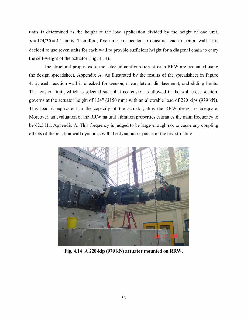
53
units is determined as the height at the load application divided by the height of one unit,
1.430124 ==n units. Therefore, five units are needed to construct each reaction wall. It is
decided to use seven units for each wall to provide sufficient height for a diagonal chain to carry
the self-weight of the actuator (Fig. 4.14).
The structural properties of the selected configuration of each RRW are evaluated using
the design spreadsheet, Appendix A. As illustrated by the results of the spreadsheet in Figure
4.15, each reaction wall is checked for tension, shear, lateral displacement, and sliding limits.
The tension limit, which is selected such that no tension is allowed in the wall cross section,
governs at the actuator height of 124" (3150 mm) with an allowable load of 220 kips (979 kN).
This load is equivalent to the capacity of the actuator, thus the RRW design is adequate.
Moreover, an evaluation of the RRW natural vibration properties estimates the main frequency to
be 62.5 Hz, Appendix A. This frequency is judged to be large enough not to cause any coupling
effects of the reaction wall dynamics with the dynamic response of the test structure.
Fig. 4.14 A 220-kip (979 kN) actuator mounted on RRW.

54
221
0.0
5.0
10.0
15.0
20.0
0 100 200 300 400 500 600 700 800 900 1000 1100 1200
Actuator load [kip]
Hei
gth
[ft]
tension limit shear limit displacement limit sliding limit
Fig. 4.15 Design spreadsheet output for used RRW (1 ft = 304.8 mm, 1 kip = 4.448 kN).
4.7.2 Setup on Strong Floor
Figure 4.16 shows the experimental setup including the RRW and the test substructures on the
strong floor. The positions of the RRW and the attached actuators and test substructures are
selected according to the limitations of the space and geometry of the floor, as well as to provide
different opportunities for future test setups. In addition, this configuration allows the possibility
of using out-of-plane restraints if needed for the RC frames. During the test, the out-of-plane
displacements are monitored and it is determined that they are of insignificant amplitude in the
conducted experiments (see Section 4.5 and Fig. 4.11).
4.8 EXPERIMENTAL SETUP IMPLEMENTATION
The assembly of the test setup consists of the construction of the RRW, the attachment of the test
substructures to the strong floor, and the installation of the loading apparatus to connect the
actuators to the test substructures. This section summarizes these steps for constructing the test
setup.

55
4.8.1 Construction of RRW
The construction of the RRW consists of placing the wall units in their setup positions with a
layer of special grout between the strong floor and the lower unit, and between every two
subsequent units. High-strength steel rods are then placed in the allocated vertical tubes, aligned
through the wall height and the strong floor thickness (Fig. 4.16), and post-tensioned to the
desired load of 100 kips (450 kN) per rod. The main steps are illustrated in the photographs of
Figure 4.17.
4.8.2 Attachment of Actuator to RRW
A steel base plate serves as the interface between the actuator and the RRW. It is first installed
on the face of the RRW at the actuator intended height, then grouted and post-tensioned to
ensure perfect contact. The base plate includes threaded holes which allow its connection with
the actuator end plate. The actuator is then bolted to its end plate and connected to the hydraulic
system. Figure 4.18(a) shows the end plate installation on the RRW, and Figure 4.18(b) shows
the actuator placed in position.
4.8.3 Attachment of Test Substructures to Strong Floor
The RC frames are first placed in their specified location on the strong floor. The footing of each
RC column contains several built-in PVC tubes extending through the thickness of the footing
(Fig. 4.6). High-strength rods with an end plate from each side are passed in these tubes and
through the thickness of the strong floor. These rods are post-tensioned with a load of 100 kips
(450 kN) (Fig. 4.19). This level of post-tensioning ensures the complete fixity (with no tension
developing at the footing–strong floor interface) at any stage of lateral loading.

56
9'
16'
2'-412"
20'
OptionalN
Out-of-plane 1 Out-of-plane 2
Out-of-plane 4Out-of-plane 3
out-of-planerestraints
(a) Plan view 20'
57'
12'-6"
20", 220 kip
10'-4"
Strong floor
Actuator CL
(b) Elevation view
11'-3"
Actuator C
20'8'-6"
2' floor
L
10'-4"
Post-tensioning rod
(c) Side view
Fig. 4.16 Test setup on strong floor for test structure A (1'=304.8 mm, 1"=25.4 mm, 1 kip = 4.448 kN).

57
(a) Grout placement on strong floor (b) Transportation of an upper wall unit
(c) Grout placement between two upper
units (d) High-strength post-tensioning rod
Fig. 4.17 Construction of RRW.
(a) Installation of base plate onto face of
RRW (b) Actuator installation and connection to
base plate
Fig. 4.18 Installation of actuator at desired height.

58
Post-tensioning rod inside PVC tube to
strong floor
Loading apparatus
End plate
Post-tensioning rod inside PVC tube to
strong floor
Loading apparatus
End plate
Fig. 4.19 Loading apparatus mounted on RC bare frame.
4.8.4 Installation of Loading Apparatus
The attachment of the actuator clevises to the test substructures needs to accommodate the
application of tension and compression forces. Steel plates are positioned at each end of the RC
frame at the beam level. The plate on the actuator end of the frame provides the interface
between the actuator and the test substructure. Two steel W-beams and two angles are positioned
along the length of the RC beam of each frame (Figs. 4.19–4.20). These steel elements are
connected to the end plates using high-strength rods. The loading apparatus provides the grip
necessary to attach the actuator to the frame. In addition, the steel beams are tensioned prior to
the test, thus subjecting the RC beams to axial compression forces.
The post-tensioning forces are intended to counteract the tension forces in the steel beams
during the application of pulling loads by the actuators. Accordingly, permanent contact between
the end plates and the beam ends of the RC frame is maintained throughout the test. However,
the post-tensioning increases the cracking load of the beams and joints and may lead to a delay in
the initiation and propagation of cracking and reduced deterioration of the joints. Moreover, the
applied displacement in HS, which is constant along the length of the RC beam, does not exactly
simulate the deformation corresponding to the inertial forces in the ST test. In this latter test, the
inertial force is distributed uniformly within the area of the RC slab and results in a uniformly

59
distributed lateral load along the length of the RC beams. Therefore, two sources of discrepancy
between the ST test and the pseudo-dynamic test are attributed to the way the test substructures
are loaded, namely (1) the application of a constant displacement versus a uniformly distributed
lateral load and (2) the post-tensioning of the RC beams causing an increase in the cracking load
along the RC beam and at beam-to-column joints. The effects of these two sources are discussed
in the comparison between the ST and HS tests at the different phases of the experiment in
Chapter 8.
hs steel rod
24.0"
RC beam
End plate
rod holes
End plate RC slabL-sectionwasher
24.0
"
28.5
"
26.0"26.0" 138"
A
A
Plan view
Section A-A
1.0"
6.5"
8.1" 1.0"138.0"
1.0" 138.0" 1.0"
W-Section 8x35
L-Section 5x5
17.5
"
Fig. 4.20 Details of loading apparatus for test structure A (1"=25.4 mm).
A torque moment corresponding to a load of 20 kips (88.9 kN) is applied on each of the
six high-strength steel rods used in the loading apparatus (Section A-A of Fig. 4.20).
Accordingly, a total of 120 kips (533.8 kN) per RC frame is applied as post-tensioning force in
the RC beam. This load is larger than the expected maximum load to be applied on the RC frame
(Table 4.5) and translates into an axial compressive stress of less than 600 psi (4.14 N/mm2)

60
(< 13% cf ′ ) on the beam. This compressive stress, although not large, is not insignificant and is
expected to influence the behavior of the beam-to-column joints and RC beams as mentioned
above and discussed further in Chapter 8. The alignment of the end plates, which transfer the
load to the RC beam, within the beam cross section is such that the post-tensioning load resultant
is applied in the center of gravity of the combined cross section of the RC beam and slab (T-
beam), i.e., the eccentricity of the post-tensioning force is zero.
4.9 HS IDEALIZATION OF TEST STRUCTURE
An essential limitation of the HS is entailed by the method used to load the experimental
substructures. The actuators are attached to specific points on the physical substructures and it is
not practically possible to distribute the load along the inertial mass of the substructure as in the
actual case of ground shaking. Therefore, the test structure needs to be carefully idealized into a
distinct number of DOF. Subsequently, the dynamic properties are defined in terms of these
selected DOF only.
In this study, the test structure is loaded in-plane in a direction parallel to the frames.
Each frame may be represented by a large number of DOF along the length of the beam and the
height of the columns (Fig. 4.21(a)). A lumped mass is assigned to each degree of freedom, such
that the total inertial mass is represented by the selected degree of freedom. Note that the inertial
mass in this case reflects the weights of the RC columns, the RC beam and the part of the
adjacent RC slab tributary to the frame in question. Moreover, any additional weights due to
gravity loads should be also included. The higher the number of DOF, the more accurate this
idealization would be and the closer it is to the distributed nature of the inertial mass of the
frame. Although this representation may be accurate in describing the dynamic response of the
test structure, the application of the load to this large number of DOF is not practically feasible.
For simplicity and practicality, the idealization is simplified to the representation of each
frame as a single degree of freedom (SDOF) (Fig. 4.21(b)). The validity of this further
simplification is based on the assumption that the beam in each frame is rigid in the loading
direction and thus is subjected to the same displacement along its length. This allows the seismic
demand to be applied to the test structure using one actuator attached to the RC beam for each
frame.
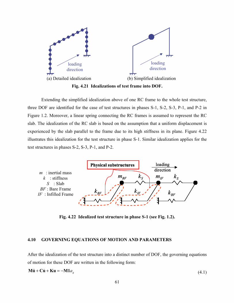
61
loading direction
loading direction
(a) Detailed idealization (b) Simplified idealization
Fig. 4.21 Idealizations of test frame into DOF.
Extending the simplified idealization above of one RC frame to the whole test structure,
three DOF are identified for the case of test structures in phases S-1, S-2, S-3, P-1, and P-2 in
Figure 1.2. Moreover, a linear spring connecting the RC frames is assumed to represent the RC
slab. The idealization of the RC slab is based on the assumption that a uniform displacement is
experienced by the slab parallel to the frame due to its high stiffness in its plane. Figure 4.22
illustrates this idealization for the test structure in phase S-1. Similar idealization applies for the
test structures in phases S-2, S-3, P-1, and P-2.
m : inertial mass k : stiffness
S : Slab BF : Bare Frame
IF : Infilled Frame
loadingdirection
Physical substructures
BFm
BFk IFk
IFmSk Sk
BFk
loadingdirection
Physical substructures
BFm
BFk IFk
IFmSk Sk
BFk
Fig. 4.22 Idealized test structure in phase S-1 (see Fig. 1.2).
4.10 GOVERNING EQUATIONS OF MOTION AND PARAMETERS
After the idealization of the test structure into a distinct number of DOF, the governing equations
of motion for these DOF are written in the following form:
gaM1KuuCuM −=++ (4.1)

62
where M is the mass matrix, C is the damping matrix, K is the stiffness matrix, 1 is the
influence vector which is a vector of ones in this case, since all the masses are assumed to be
excited by the ground motion, ga is the ground acceleration to which the test structure is
assumed to be subjected to and u , u , and u are the acceleration, velocity, and displacement
vectors, respectively, of the idealized test structure. In the following sections, the estimation of
M , C , and K are derived from the parallel ST test conducted on a test structure similar to that
of phase S-1.
4.10.1 Mass Matrix
The mass matrix represents the inertial mass present on the ST test structure. The sum of the
mass of the ST test structure and the additional mass attachments on top of the RC slab (Hashemi
and Mosalam 2006) are estimated based on the tributary areas of the floor for each frame into the
three DOF representing the test structure (Fig. 4.23). Accordingly, two similar masses are
allocated for the exterior bare frames, BFm , and one larger mass allocated for the interior infilled
frame, IFm . The resulting diagonal mass matrix becomes:
⎟⎟⎟
⎠
⎞
⎜⎜⎜
⎝
⎛=
BF
IF
BF
mm
m
000000
M (4.2)
The same procedure is applied to the test structures in phases S-2, S-3, P-1, and P-2.
mBF mBFmIF
F2B F1I F2B
Fig. 4.23 Mass allocation by tributary areas.

63
4.10.2 Damping Matrix
The damping ratio suitable for the test structure in phase S-1 is evaluated based on a pull-back
test before the ST experiments. In this pull-back test, the ST test structure is pulled from the top
RC slab causing a small deformation and then suddenly released to freely vibrate (Hashemi and
Mosalam 2007). The resulting damping ratio ζ and natural frequency nω are subsequently
estimated. For simplicity in HS, damping is assumed to be first-mode mass proportional (Chopra
2001), as follows:
nωζ MC 2= (4.3)
4.10.3 Stiffness Matrix
The stiffness matrix is derived from the idealized form of the test structure (Fig. 4.22).This yields
the stiffness matrix below:
⎟⎟⎟
⎠
⎞
⎜⎜⎜
⎝
⎛
+−−+−
−+=
SBFS
SSIFS
SSBF
kkkkkkk
kkk
02
0K (4.4)
where BFk , IFk , and Sk are the stiffness of the bare frame, infilled frame and slab, respectively.
This stiffness matrix can be expressed as the sum of two matrices FK and SK , where:
⎟⎟⎟
⎠
⎞
⎜⎜⎜
⎝
⎛
−−−
−=
⎟⎟⎟
⎠
⎞
⎜⎜⎜
⎝
⎛=
+=
110121
011 and
000000
SS
BF
IF
BF
F
SF
kk
kk
KK
KKK
(4.5)
Noting that the product uKR FF = is a 3×1 vector representing the restoring forces to be
measured from the test substructures, only one exterior bare frame is tested together with the
interior infilled frame for phase S-1. From symmetry, the restoring force in the other
(numerically simulated) bare frame is estimated as having the same value as the one that is
physically tested. Accordingly, the equations of motion are written in the form:
gSF aM1uKRuCuM −=+++ (4.6)

64
For phases S-2, S-3, P-1, and P-2, the physical substructure consists of one RC bare
frame. The RC slab, due to its high lateral stiffness (see Section 4.12) forces the three RC bare
frames of the test structure to be subjected to almost the same displacement demand. The
restoring forces in each of the other two numerically simulated frames are thus taken the same as
the measured restoring force from the physically tested substructure. Note that the inertial forces
are different for the URM infilled frame and bare frames because of differences in the associated
masses.
4.11 INITIAL STIFFNESS ESTIMATION FOR PHYSICAL SUBSTRUCTURES
A set of pull-back tests is performed on each of the two RC frames in the direction of their plane.
While pull-back tests are useful in evaluating the damping properties of the structure as well as
its initial stiffness, the damping properties in this HS test are specified in the numerical-
integration algorithm, based on the measured values from the structure tested with the proper
mass on the ST. Therefore, the only results sought from these pull-back tests are the initial
stiffness of the RC frames. The estimated values serve as guidelines before starting the HS test to
estimate the modal frequencies (see Section 4.13) and the stiffness matrix in its undamaged state,
which is needed to initiate the simulation using the numerical-integration algorithm, discussed in
Section 6.1.
A load cell is connected in series with a lever chain hoist and a short piece of 1/4" (6.4
mm) steel rod between the reaction wall and the RC frame (Fig. 4.24). The chain is used to load
the attachment to the desired load and the steel rod is cut abruptly to release the frame, which is
left to vibrate freely. The measured force and displacement while loading are used to evaluate the
stiffness. The test is performed on the URM infilled RC frame (F1I) with post-tensioned columns
using a load of 5 kips (22.2 kN) and on the RC bare frame before post-tensioning (F2BU) and
after post-tensioning the columns (F2B) with a load of 3 kips (13.3 kN) in both cases. The test is
performed twice for each case and the stiffness is evaluated as the average of the two results;
refer to the summary of results in Table 4.6. Note that the ratio between the stiffness of the URM
infilled and bare RC frames is rather high (21.8) compared to what is typically found in the
literature (Mosalam et al. 1997b, c, and d). This may be attributed to the fact that the interface
between the URM infill wall and the surrounding RC frame remained intact at these low levels
of lateral forces. Once hairline separation cracks form along the frame/wall interface when the

65
RC frame is loaded to a magnitude of deformation capable of overcoming the bond at the
interface, the stiffness is expected to reduce significantly.
Load cellLever chain
hoist1/4 in dia. rod Load cellLever chain
hoist1/4 in dia. rod Load cellLever chain
hoist1/4 in dia. rod Load cellLever chain
hoist1/4 in dia. rod
Fig. 4.24 Pull-back test setup.
Table 4.6 Pull-back test results for substructures of test structure A.
Frame F1I F2B F2BU Stiffness from test 1 [kips/in. (kN/mm)] 840 (147.1) 40.4 (7.08) 37.9 (6.64) Stiffness from test 2 [kips/in. (kN/mm)] 950 (166.4) 41.6 (7.29) 37.7 (6.60)
Average stiffness [kips/in. (kN/mm)] 895 (156.7) 41.0 (7.18) 37.8 (6.62)
The initial stiffness is re-estimated during a set of preliminary runs applied before the
start of phase S-1 (see Fig. 1.2) to have a more realistic estimation of the initial stiffness. These
low-level preliminary runs are aimed at estimating the integration time step tΔ to be used in the
HS experiments (see Section 4.14) and for obtaining a more representative estimate of the initial
stiffness. Figure 4.25 shows the restoring force of the URM infilled RC frame versus its lateral
displacement for the fourth and last of these preliminary runs. The initial stiffness is estimated by
computing an average tangent stiffness over the time history, using the least-squares method to

66
obtain a best linear fit for the initial stiffness but excluding the major loading cycles beyond
0.04" (1 mm). The value of ≈K 700 kips/in. (122.6 kN/mm), i.e., 78% of the average stiffness
obtained from the pull-back test, is determined from all four runs and is therefore adopted as the
initial stiffness in the numerical-integration algorithm.
-0.1 -0.05 0 0.05 0.1-80
-40
0
40
80
Displacement [in]
Forc
e [k
ips]
-2 0 2
-300
-200
-100
0
100
200
300
Displacement [mm]
Forc
e [k
N]
K = 703 kips/in
Fig. 4.25 Restoring force versus lateral displacement of URM infilled RC frame from preliminary run (1 kip/in. = 0.175 kN/mm).
4.12 RC SLAB STIFFNESS ESTIMATION
The RC slab is assumed to have in-plane linear behavior within the range of deformation
introduced by the applied earthquake motions. To determine the value of the in-plane stiffness, a
theoretical value is calculated and verified against the experimental results from the ST tests as
described below.
4.12.1 Theoretical In-Plane Stiffness of RC Slab
To estimate a theoretical value of the RC slab in-plane stiffness, the slab is assumed to act as a
shear element between the two adjacent frames (Fig. 4.26). Accordingly, the theoretical stiffness
Sk is estimated as follows:

67
LbtG
LA
LAFFkS =×
Δ=
Δ= (4.7)
( )C
CELAFG
νγτ
+=
Δ==
12 (4.8)
where CE and Cν are the concrete elastic Young’s modulus and Poisson’s ratio, respectively.
Other parameters in the above equations are shown in Figure 4.26. These parameters are
substituted by their estimated values listed in Table 4.7, and the resulting stiffness is evaluated as
Sk =16500 kips/in. (2889.6 kN/mm).
b
Lt
Δ
Fγ
tbA =
Fig. 4.26 RC slab stiffness estimation (not to scale).
Table 4.7 Values of parameters used in RC slab in-plane stiffness estimation.
Parameter CE [ksi (kN/mm2)] Cν t [in. (mm)] b [in. (mm)] L [in. (mm)]
Value 4000 (700.5) 0.2 3.75 (95) 192 (4877) 72 (1829)
4.12.2 Experimental In-Plane Stiffness for RC Slab
Several runs are executed in the HS setup on the test structure of phase S-1 subjected to the low-
level seismic motion, TAR level 2 (TAR-2) in Table 4.2. The test is repeated four times using
different values for the stiffness of the RC slab corresponding to 1%, 3%, 10%, and 100% of the
theoretical value Sk = 16500 kips/in. (2889.6 kN/mm) . The results are plotted in Figure 4.27 on
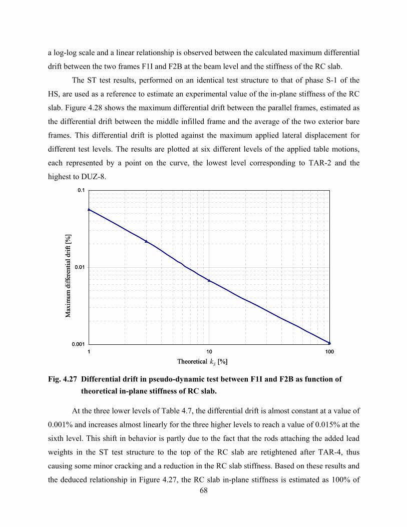
68
a log-log scale and a linear relationship is observed between the calculated maximum differential
drift between the two frames F1I and F2B at the beam level and the stiffness of the RC slab.
The ST test results, performed on an identical test structure to that of phase S-1 of the
HS, are used as a reference to estimate an experimental value of the in-plane stiffness of the RC
slab. Figure 4.28 shows the maximum differential drift between the parallel frames, estimated as
the differential drift between the middle infilled frame and the average of the two exterior bare
frames. This differential drift is plotted against the maximum applied lateral displacement for
different test levels. The results are plotted at six different levels of the applied table motions,
each represented by a point on the curve, the lowest level corresponding to TAR-2 and the
highest to DUZ-8.
0.001
0.01
0.1
1 10 100
Theoretical [%]Sk
Max
imum
diff
eren
tial d
rift [
%]
0.001
0.01
0.1
1 10 100
Theoretical [%]Sk
Max
imum
diff
eren
tial d
rift [
%]
Fig. 4.27 Differential drift in pseudo-dynamic test between F1I and F2B as function of theoretical in-plane stiffness of RC slab.
At the three lower levels of Table 4.7, the differential drift is almost constant at a value of
0.001% and increases almost linearly for the three higher levels to reach a value of 0.015% at the
sixth level. This shift in behavior is partly due to the fact that the rods attaching the added lead
weights in the ST test structure to the top of the RC slab are retightened after TAR-4, thus
causing some minor cracking and a reduction in the RC slab stiffness. Based on these results and
the deduced relationship in Figure 4.27, the RC slab in-plane stiffness is estimated as 100% of

69
the theoretical value of Sk up to TAR-4, corresponding to 0.001% differential drift and for
simplicity 10% of Sk thereafter, corresponding to approximately 0.007% differential drift. It is
important to note the ratio between differential drift and global drift at the beam level. For the
strongest motion DUZ-8, this ratio is calculated as 1/169, implying that the RC slab in the ST
experiment acted as a rigid diaphragm between the RC frames and forced them to be subjected to
almost the same amount of lateral deformation. In other words, the first natural mode of
vibration dominates the response of the test structure. The natural vibration modes are discussed
in more details in the next section.
0 0.5 1 1.5 2 2.5 30
0.005
0.01
0.015
0.02
Displacement [in]
Diff
eren
tial d
rift [
%]
20 40 60
Displacement [mm]
TAR-2
TAR-4 TAR-6
DUZ-7
DUZ-8
and TAR-3
0 0.5 1 1.5 2 2.5 30
0.005
0.01
0.015
0.02
Displacement [in]
Diff
eren
tial d
rift [
%]
20 40 60
Displacement [mm]
TAR-2
TAR-4 TAR-6
DUZ-7
DUZ-8
and TAR-3
Fig. 4.28 Differential drift in dynamic (ST) tests against applied maximum lateral displacement.
4.13 PARAMETERS OF EQUATIONS OF MOTION
At this point, all of the properties of the test structure are determined for the structure in phase S-
1 (see Fig. 1.2). These properties are summarized in Table 4.8 with the parameters defined in
previous sections. The natural modes of vibration are determined by solving the following
eigenvalue problem (Chopra 2001):
nnn φλφ MK = (4.9)

70
where K and M are the stiffness and mass matrices of the test structure, nφ is the modal shape
vector, and 2nn ωλ = are the eigenvalues with nω as the natural frequencies. For the three DOF
system studied, the dynamic response is governed by three natural modes of vibration with
different participation factors (Chopra 2001), i.e., 31 ≤≤ n . The natural period is defined as
nnT ωπ2= . The results of the modal properties are summarized in Table 4.9 in the case of test
structure A in phase S-1 (see Fig. 1.2), and Figure 4.29 describes the corresponding mode
shapes.
-1 -0.5 0 0.5 10
0.5
1
-1 -0.5 0 0.5 10
0.5
1
-1 -0.5 0 0.5 10
0.5
1
Normalized lateral displacement
B1
I
B2
Mode shape 1
Mode shape 2
Mode shape 3
Nor
mal
ized
hei
ght -1 -0.5 0 0.5 1
0
0.5
1
-1 -0.5 0 0.5 10
0.5
1
-1 -0.5 0 0.5 10
0.5
1
Normalized lateral displacement
B1
I
B2
Mode shape 1
Mode shape 2
Mode shape 3
Nor
mal
ized
hei
ght
B1 B2I
B1 B2I
B1 B2I
Fig. 4.29 Mode shapes for test structure A in phase S-1.
Table 4.8 Estimated parameters for test structure A in phase S-1.
Parameter BFm [kips-
sec2/in. (kN-sec2/mm)]
IFm [kips-sec2/in. (kN-sec2/mm)]
ζ [%]
BFk [kips/in.
(kN/mm)]
IFk [kips/in. (kN/mm)]
Sk * [kips/in.
(kN/mm)]
Value 0.106 (0.019)
0.070 (0.012) 6.2 41
(7.2) 700
(122.6) 16500
(2889.6) * For levels TAR-4 or lower and reduced to 10% of this value for higher levels

71
Table 4.9 Natural frequencies and periods for test structure A in phase S-1.
Mode 1 2 3 nω (rad/sec) 61.3 486.3 742.6
nf (Hz) 9.80 76.92 117.65
nT (sec) 0.1020 0.0130 0.0085
4.14 INTEGRATION TIME-STEP ESTIMATION
Ideally, the integration time step is chosen as small as possible to yield the most accurate
numerical integration. However, typically, it is required to capture the response of the test
structure in its major influential modes, which does not necessarily require that extreme level of
accuracy for the choice of the integration time step. Another controlling factor in the choice of
the numerical-integration time step may be a condition of stability (see Section 2.3). Since the
selected algorithm is unconditionally stable for test structures with a softening stiffness
(Nakashima et al. 1990), this stability condition is no longer a limitation. To accurately capture
the response, the numerical-integration time step tΔ is selected to be less than 10T , where T is
the smallest natural period of the test structure corresponding in this case to the third mode, 3T =
0.0085 sec, thus tΔ = 0.0008 sec is considered.
To examine the choice of the numerical-integration time step, the low-level strong
motion, TAR-2, is applied on the test structure in phase S-1 four times using different integration
time steps, namely tΔ = 0.0008, 0.002, 0.0025, and 0.005 sec. Figure 4.30 illustrates the
corresponding responses, which show minimal differences when comparing the displacement
time histories. The fast Fourier transform plots are especially revealing, since the second and
third modes do not show any noticeable influence in the response, and the peaks recorded are in
the first mode (9.8 Hz), at about 1T = 0.1 sec (10 Hz) or higher (< 10 Hz frequency). This finding
is in agreement with the role of the stiff RC slab in minimizing the response in the second and
third modes of vibration. This in turn allows increasing the integration time step to tΔ = 0.0025
sec when applying HS to test structure A in phase S-1. For other phases, where the URM infill
wall is removed and the test structure is much less stiff, tΔ = 0.005 sec is adopted with high
accuracy.

72
0 5 10 15-0.1
0
0.1
0 5 10 15-0.1
0
0.1
0 5 10 15-0.1
0
0.1
0 5 10 15-0.1
0
0.1
Time [sec]
Dis
plac
emen
t [in
]
Dis
plac
emen
t [m
m]
2.5
-2.5
2.5
-2.5
2.5
-2.5
2.5
-2.5
0.0008t =Δ
0.002t =Δ
0.0025t =Δ
0.005t =Δ
0 5 10 15-0.1
0
0.1
0 5 10 15-0.1
0
0.1
0 5 10 15-0.1
0
0.1
0 5 10 15-0.1
0
0.1
Time [sec]
Dis
plac
emen
t [in
]
Dis
plac
emen
t [m
m]
2.5
-2.5
2.5
-2.5
2.5
-2.5
2.5
-2.5
0.0008t =Δ
0.002t =Δ
0.0025t =Δ
0.005t =Δ
0008.0=Δt
002.0=Δt
0025.0=Δt
005.0=Δt
0
0
0
0
0 5 10 15-0.1
0
0.1
0 5 10 15-0.1
0
0.1
0 5 10 15-0.1
0
0.1
0 5 10 15-0.1
0
0.1
Time [sec]
Dis
plac
emen
t [in
]
Dis
plac
emen
t [m
m]
2.5
-2.5
2.5
-2.5
2.5
-2.5
2.5
-2.5
0.0008t =Δ
0.002t =Δ
0.0025t =Δ
0.005t =Δ
0 5 10 15-0.1
0
0.1
0 5 10 15-0.1
0
0.1
0 5 10 15-0.1
0
0.1
0 5 10 15-0.1
0
0.1
Time [sec]
Dis
plac
emen
t [in
]
Dis
plac
emen
t [m
m]
2.5
-2.5
2.5
-2.5
2.5
-2.5
2.5
-2.5
0.0008t =Δ
0.002t =Δ
0.0025t =Δ
0.005t =Δ
0008.0=Δt
002.0=Δt
0025.0=Δt
005.0=Δt
0
0
0
0
10-2
10-1
0
0.5
1
1.5x 10
-3
10-2
10-1
0
0.5
1
1.5x 10
-3
10-2
10-1
0
0.5
1
1.5x 10
-3
10-2
10-1
0
0.5
1
1.5x 10
-3
Period [sec]
FFT
ampl
itude
0.0008t =Δ
0.002t =Δ
0.0025t =Δ
0.005t =Δ
10-2
10-1
0
0.5
1
1.5x 10
-3
10-2
10-1
0
0.5
1
1.5x 10
-3
10-2
10-1
0
0.5
1
1.5x 10
-3
10-2
10-1
0
0.5
1
1.5x 10
-3
Period [sec]
FFT
ampl
itude
0.0008t =Δ
0.002t =Δ
0.0025t =Δ
0.005t =Δ
0008.0=Δt
002.0=Δt
0025.0=Δt
005.0=Δt
10-2
10-1
0
0.5
1
1.5x 10
-3
10-2
10-1
0
0.5
1
1.5x 10
-3
10-2
10-1
0
0.5
1
1.5x 10
-3
10-2
10-1
0
0.5
1
1.5x 10
-3
Period [sec]
FFT
ampl
itude
0.0008t =Δ
0.002t =Δ
0.0025t =Δ
0.005t =Δ
10-2
10-1
0
0.5
1
1.5x 10
-3
10-2
10-1
0
0.5
1
1.5x 10
-3
10-2
10-1
0
0.5
1
1.5x 10
-3
10-2
10-1
0
0.5
1
1.5x 10
-3
Period [sec]
FFT
ampl
itude
0.0008t =Δ
0.002t =Δ
0.0025t =Δ
0.005t =Δ
0008.0=Δt
002.0=Δt
0025.0=Δt
005.0=Δt
(a) Displacement time history (b) fast Fourier transform for displacement
Fig. 4.30 Comparison of response for TAR-2 using different integration time steps Δt in HS.
4.15 SUMMARY
The shaking table experiments, which preceded the hybrid simulation on an identical test
structure, serve as benchmarks for the hybrid simulation experiments. Therefore, in all the steps
concerning the construction of the hybrid simulation experiments, measures are taken to
eliminate any avoidable deviations between the two tested structures. The hybrid simulation
system test structure in question is divided into physically tested substructures and numerically
modeled substructures. For each phase of the experimental program (see Fig. 1.2), these
substructures are identified and the basis for modeling the computational part is presented. The
physical substructures used in all tests are two ¾-scale RC frames, one a bare frame, the other

73
infilled using an URM wall. The structural design of the RC frames is detailed, as well as their
construction, material properties, and instrumentation. The experimental setup design in the
structural laboratory is discussed, including the design of the reconfigurable reaction walls, their
positions on the laboratory strong floor and the selection of the actuators. A loading apparatus is
designed to attach the actuators to the RC frames while avoiding the creation of any gaps
between the test substructures and the used actuators during the push/pull loading actions of the
actuators. A set of low-amplitude hybrid simulation runs on test structure A in phase S-1 are
performed to evaluate key parameters in the equations of motion, namely the initial stiffness of
the test structure, the RC slab in-plane stiffness Sk , and the integration time step tΔ .

5 Test Structure B
The second test structure presented in this chapter consists of two large substructures of a ST
experiment conducted at UCB. The ST test structure is briefly presented along with the selection
of the strong motions applied during different phases of the ST experiment. This chapter
describes the physical substructures of the HS test structure including design, construction, and
instrumentation. Moreover, the test setup on the strong floor is discussed in terms of its design
and assembly. Similar to test structure A, discussed in the previous chapter, the development of
the computational part of the HS for test structure B is discussed. This includes the idealization
of test structure B, the formulation of the governing equation of motion, and the estimation of
some key parameters in this equation of motion.
5.1 ST TEST STRUCTURE
The seismic vulnerability of timber structures was demonstrated during recent earthquakes in
California. In particular, a wood-frame building with an open front due to tuck-under parking is
characterized by a soft first story (Mosalam et al. 2002; Mosalam and Mahin 2007). The building
used in the ST experiment is a hypothetical two-story single-family “house-over-garage”
representing the plethora of houses in San Francisco, California, constructed in the 1930s. The
ST experiment is carried out on the full-scale two-story structure on the seismic simulator test
facility of UCB (Fig. 5.1).

76
NNN NNN
(a) Northeast corner (b) Northwest corner
Fig. 5.1 Two-story wood house over garage on ST.
5.2 TEST STRUCTURE DESIGN
The design of the shear walls in the ST test structure is presented in this section and is adopted
for the HS physical substructure, discussed in Section 5.4. The plan dimensions are 19' 6"×13' 6"
(5944 mm×4115 mm) (Fig. 5.2). The height is 18' 6" (5639 mm) from the bottom to the highest
point of the roof, which is partially covered by a parapet of 2' 10" (864 mm) height (Fig. 5.3(a)).
The shear walls are constructed using 1×12 shiplap siding (3-8d common nails per stud crossing)
reinforced by V-shaped 2×4 diagonal blocking between studs (2-16d toe common nails) (Figs.
5.3(b) and 5.5). The two longitudinal (north and south) shear walls are 19' 6"×9' (5944 mm×2743
mm) with 2×4 studs at 16" (406 mm) spacing. The studs are end nailed (2-16d common) to
double 2×4 top plates and toe nailed (3-16d common) to 3×6 sill plate with 1/2"×12" (13
mm×305 mm) anchor bolts at 4' (1219 mm) spacing with 1½" (38 mm) cut washers and square
nuts to connect the sill plates to RC wall footings (Fig. 5.4). All lumber is Douglas Fir-Larch.

77
5.3 STRONG MOTION SELECTION
In the ST experiment, Loma Prieta, Los Gatos station, 1989 (LPG) was chosen to match the
design basis earthquake (DBE) (10% probability of exceedance in 50 years) and upper-bound
earthquake (UBE) (10% probability of exceedance in 100 years) levels of shaking. This ground
motion is scaled to match design spectra of a stiff site in the Richmond district of San Francisco.
Both fault-normal (FN) and fault-parallel (FP) components of this chosen ground motion are
presented in Table 5.1. While on the ST, the test structure was subjected to a bidirectional
motion, the HS test structure is tested in one direction parallel to the shear walls (E-W direction
on the ST). The ground motion is scaled to generate different levels of intensity as listed in Table
5.2. As for test structure A in Chapter 4, the accelerations are measured on the ST during each
run and applied in the HS, rather than the original scaled input motions. Prior to use in the HS
experiments, these measured table accelerations are subjected to a low-pass filter at 25 Hz cut-
off frequency.
Fig. 5.2 Wood house first-floor plan.

78
(a) East wall elevation
(b) North wall elevation
Fig. 5.3 Wood house elevation views.

79
Fig. 5.4 Design details of wood house.
Fig. 5.5 Blocking used to brace shear-wall framing of test structure B.

80
Table 5.1 Loma Prieta 1989, Los Gatos Station strong motion (LPG).
Design Basis Earthquake (DBE) Upper-bound Earthquake (UBE) Direction PGA
(g) PGV [in./sec
(mm/sec)] PGD [in.
(mm)] PGA (g)
PGV [in./sec (mm/sec)]
PGD [in. (mm)]
Fault Normal
0.42 21.09 (535.7) 3.77 (95.8) 0.46 25.43 (645.9) 5.06 (128.5)
Fault Parallel
0.38 16.21 (411.7) 2.37 (60.2) 0.57 20.64 (524.3) 3.10 (78.7)
Table 5.2 Scale factors for different levels of input ground motion (fault normal) except as noted.
Level 1 2 3 4 5 6* Motion Scale 0.10×UBE 0.25×UBE 0.50×UBE 1.00×DBE 1.00×UBE 1.00×UBE
* Fault normal followed by fault parallel
5.4 TEST STRUCTURE IN HS
The HS test structure B is presented in this section. The idealization leading to the development
of the numerical model and the selection of the physical substructure, as well as the design of the
experimental setup and the instrumentation of the test structure are discussed.
5.4.1 Idealization
Since in the ST experiment, the second story behaved very closely to a rigid mass atop the first-
story shear walls, the two longitudinal (north and south) shear walls are constructed at full scale
and treated in HS as the physical substructure (Figs. 5.6 and 5.7(a)). The test structure for the HS
is idealized as a SDOF structure excited by a unidirectional motion parallel to the E-W direction
where the north (N) direction is identified in Figures 5.2 and 5.6(a)).
5.4.2 Experimental Setup
A rigid steel horizontal frame (Fig. 5.8) connects the two shear walls to a single dynamic
actuator as identified in Figures 5.6 and 5.7(c)). Furthermore, three high-strength steel rods,

81
shown in Figure 5.7(b), each linked to a load cell in series, are connected to the strong floor at
one end and the loading steel frame at the other end and are post-tensioned to simulate the
gravity load present in the case of the ST test structure. It should be noted that these post-
tensioned steel rods provided some resistance to overturning, leading to a change of the applied
gravity loads by these rods. From the load cell measurements during the application of the strong
motion LPG level 6 (LPG-6) (see Section 5.3), the total variation in the force applied by these
rods was between 7.3 kips (32.5 kN) and 15.0 kips (66.7 kN), while the total initial value of the
gravity load applied by these rods is 10.5 kips kN (46.7 kN) (Fig. 5.9). The height of the test
structure, including the RC foundation, requires the construction of a five-unit high RRW with
total height of 12' 6" (3810 mm). The maximum load of the combined two shear walls is not
expected to exceed 30 kips (5.3 kN), and therefore the RRW limits are certainly not exceeded
(see Section 4.7.1). The same 220 kips (979 kN) dynamic actuator used in the case of the RC
frame structure for test structure A, Chapter 4, is selected for use with test structure B (see Table
3.1).
Out-of-plane West Out-of-plane East
In-plane North
In-plane South
Slip North
Slip South
W14
x90
W14
x90
W14
x90
19'-6"
6'-10 116"TS 4x4 TS 4x4
(a) Plan view and instrumentation
Slip N & S
In-plane N & S
8'-6"8'STUD LENGTH9'-61
2"
1'-2"
(b) Elevation view and instrumentation
Fig. 5.6 Test setup and instrumentation on strong floor for test structure B (1'=304.8 mm, 1"=25.4 mm)

82
(a) Overview of HS physical substructure (b) Post-tensioned high-strength steel rod
monitored using load cell
(c) Horizontal loading steel frame (d) Detail of shear wall with shiplap
siding
Fig. 5.7 HS physical substructure for test structure B.
5.4.3 Instrumentation
In addition to the internal displacement transducer in the actuator, the in-plane deformations of
the two tested shear walls (north and south) are measured using two wire potentiometers fixed to
the RRW on one end and the two shear walls on the other end (Fig. 5.6). The measurements
serve as a check of the amount of torsion, if any, in the tested shear walls, which would be

83
manifested in the form of a differential deformation between the two rigidly connected shear
walls. Four additional displacement transducers monitor the motion at the bases of the shear
walls (north and south) to check if any sliding occurs and out-of-plane movements of the east
and west ends (Fig. 5.6(a)). These measurements along with the load cells connected in series
with the steel three vertical high-strength rods and the horizontal actuator are recorded using the
data-acquisition system described in Section 3.6.
W
14x9
0
W14
x90
W14
x90
TS 4x4 TS 4x4
3/8
TS4x4 to W14 and L6x63/8
W14 to L6x6TYPICAL
TYPICAL
L6x6x1/2"
5/8"Ø HOLES
(a) Plan view
5/8"Ø HOLES, 16" O.C.3/8
L6x6x1/2"
(b) Elevation view
Fig. 5.8 Loading frame for test structure B (1'=304.8 mm, 1"=25.4 mm).
A cyclic preliminary test was conducted before the application of the strong motion
sequence described later on identical shear walls to the ones being tested using HS with the
purpose of assessing the test setup. Figure 5.10 shows the displacement signal applied on the
shear walls with a maximum displacement of 10 in. (254 mm) in this cyclic preliminary test. In
this figure, the deformation of the two shear walls are plotted and show almost no difference,
implying that the test structure was not subjected to any torsional effects. The sliding time
histories at the bases of the two shear walls are plotted in Figure 5.11, confirming practically

84
motionless bases. The out-of-plane measurements in Figure 5.12 record maximum out-of-plane
drifts of 0.55% and 1.1% from potentiometers 1 and 2, respectively, Figure 5.6, compared to the
10% imposed in-plane drift. These drifts are estimated as the out-of-plane deformations
normalized by the story height, i.e., 8' 6" (2590 mm) and are viewed as small deformations
considering the long length of the shear wall of 19' 6" (5944 mm).
0 5 10 15 200
5
10
15
Time [sec]
Forc
e [k
ips]
0
20
40
60
Forc
e [k
N]
0200 5 10 15 20
0
5
10
15
Time [sec]
Forc
e [k
ips]
0
20
40
60
Forc
e [k
N]
020
Fig. 5.9 Vertical force variation in post-tensioned steel rods in LPG-6.
0 500 1000 1500 2000
-10
-5
0
5
10
Time [sec]
Stor
y dr
ift [%
] North wallSouth wall
Fig. 5.10 Displacement time history for preliminary test.
0 500 1000 1500 2000
-0.02
-0.01
0
0.01
0.02
Time [sec]
Slid
ing
[in]
North wallSouth wall
-0.5
-0.25
0
0.25
0.5
Slid
ing
[mm
]
Fig. 5.11 Sliding at bases of shear walls in preliminary test.

85
0 500 1000 1500 2000-2
-1
0
1
2
Time [sec]
Out
-of-p
lane
drif
t [%
]Potentiometer 1 (west)Potentiometer 2 (East)
Fig. 5.12 Out-of-plane drift of north shear wall in preliminary test.
5.5 GOVERNING EQUATION OF MOTION AND PARAMETERS
As discussed in the previous section, the HS test structure is idealized as a SDOF system with the
two north and south shear walls being the physical substructure. The equivalent inertial mass, m ,
is therefore taken as that of the entire building tested on the ST. Mass proportional damping is
selected with damping ratio ζ =5% to match the pull-back test results from the ST test structure.
The initial stiffness k for the undamaged test structure and is estimated from preliminary low-
level ST tests (Table 5.3). The equation of motion governing the dynamics of the test structure
becomes,
gumkuumum −=++ ωζ2 (5.1)
where u , u , and u are the displacement, velocity, and acceleration of the test structure,
respectively, and gu is the imposed ground acceleration. Based on the estimated parameters of
the governing equation of motion, the natural frequency of the undamaged test structure is
estimated as mk=ω and the natural period is ωπ2=T . The integration time step adopted is
005.0=Δt sec, corresponding to the sampling frequency in the ST experiment where the motion
was recorded. This selected tΔ comfortably satisfies the stability and accuracy requirements for
capturing the fundamental dynamic response.

86
Table 5.3 Estimated parameters for HS of test structure B.
Parameter m
[kips-sec2/in. (kN-sec2/mm)]
ζ (%)
k [kips/in.
(kN/mm)]
ω (rad/sec)
f (Hz)
T (sec)
tΔ (sec)
Value 0.065 (0.011) 5.0 15 (2.6) 15.2 2.5 0.4 0.005
5.6 SUMMARY
A shaking table experiment is conducted on a full-scale two-story wood house over a garage
typically characterized as a “soft” first story. The corresponding hybrid simulation test structure
is idealized as a single-degree-of-freedom model where the two longitudinal first-story shear
walls constitute the physical substructures and are tested with in-plane loading. The structural
design of the shear walls is detailed, as well as their instrumentation. Key parameters in the
governing equation of motion and the numerical-integration algorithm time step are also
estimated.

6 New Advances in Hybrid Simulation
This chapter starts by presenting the numerical-integration algorithm in DC to provide the
necessary background for discussing the newly developed advances in HS in this report. Two
procedures are developed, namely (1) feed-forward error compensation in DC and (2) mixed-
variables control (force/displacement) which requires the development of a new FC algorithm. A
study of the developed algorithm and practical implementation strategies are also discussed.
6.1 INTEGRATION ALGORITHM IN DC
The integration algorithm solves the governing equations of motion in a step-by-step manner. In
the present study, a variation of the implicit Newmark’s method by Hilber et al. (1977), namely
the α -method, as presented by Shing et al. (1991), is used to solve the governing equations of
motion. In addition, an operator-splitting scheme (Nakashima et al. 1990) is used, where the
stiffness matrix is divided into numerical and experimental parts. While the numerical part may
be solved implicitly, the experimental part is solved using an explicit predictor-corrector method,
thus eliminating the need for an iterative procedure, which is not suitable for the experimental
part. At any time step 1+i , the equations of motion are discretized into the form,
( ) ( ) ( ) iiiiiii PPRRuCuCuM αααααα −+=−++−++ ++++ 1111 111 (6.1)
where 1+iP is the excitation force acting on the numerical model of the structure, 1+iR is the total
restoring force of the structure, and α is an integration parameter. Note that in the case of
seismic excitation,
gaM1P −= (6.2)
Variables in the above two equations have been defined in previous chapters when
discussing the governing equations of motion of test structures A and B. Let us define u~ and u
as the predictor and corrector displacements, respectively, such that:
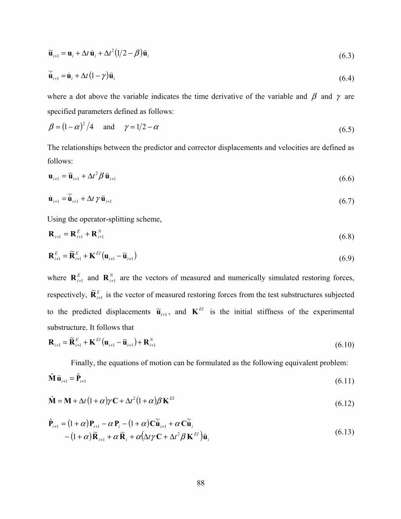
88
( ) iiii tt uuuu β−Δ+Δ+=+ 21~ 21 (6.3)
( ) iii t uuu γ−Δ+=+ 1~1 (6.4)
where a dot above the variable indicates the time derivative of the variable and β and γ are
specified parameters defined as follows:
( ) αγαβ −=−= 21 and41 2 (6.5)
The relationships between the predictor and corrector displacements and velocities are defined as
follows:
12
11~
+++ Δ+= iii t uuu β (6.6)
111~
+++ Δ+= iii t uuu γ (6.7)
Using the operator-splitting scheme, Ni
Eii 111 +++ += RRR (6.8)
( )1111~~
++++ −+= iiEIE
iEi uuKRR (6.9)
where Ei 1+R and N
i 1+R are the vectors of measured and numerically simulated restoring forces,
respectively, Ei 1
~+R is the vector of measured restoring forces from the test substructures subjected
to the predicted displacements 1~
+iu , and EIK is the initial stiffness of the experimental
substructure. It follows that
( ) Niii
EIEii 11111
~~+++++ +−+= RuuKRR (6.10)
Finally, the equations of motion can be formulated as the following equivalent problem:
11ˆˆ
++ = ii PuM (6.11)
( ) ( ) EItt KCMM βαγα +Δ++Δ+= 11ˆ 2 (6.12)
( ) ( )( ) ( ) i
EIii
iiiii
tt uKCRR
uCuCPPP
βγααααααα
21
111~~1
~~11ˆ
Δ+Δ+++−
++−−+=
+
+++ (6.13)

89
where Ni
Eii 111
~~~+++ += RRR and N
i 1~
+R is the vector of numerically simulated restoring forces
corresponding to the predicted displacements 1~
+iu . In the case of 0=α , no numerical damping
is introduced and the method reduces to the average acceleration method, where 41=β and
21=γ , which is the adopted case in the experimental investigation in the present study. The
implementation of the integration algorithm is shown in Figure 6.1. The equilibrium in this case
is satisfied at the end of each integration time step by calculating the acceleration vector 1+iu
from Equation (6.11), after measuring 1~
+iR and substituting in Equation (6.13). The corrected
displacements 1+iu from Equation (6.6) are used to calculate a corresponding Ei 1+R using the
assumed initial stiffness EIK for the experimental part from Equation (6.9) (without applying the
load on the physical substructure) as well as a corrected Ni 1+R using the model of the numerical
substructures. Note that the predicted displacement 2~
+iu applied in the following time step is
calculated from Equation (6.3) using the corrected displacement 1+iu from the preceding time
step. Therefore, in the process of applying 2~
+iu on the physical substructure, the substructure is
subjected to the calculated corrected displacement 1+iu before continuing to 2~
+iu .
Pred
ictio
nC
orre
ctio
n
Compute 1i+1i+ uu ~,~
Compute 1i+P
Start
1+= ii
End max1 ii ≥+ NoYes
Apply to the physical specimen and measure the force feedback
1i+u~
Determine total restoring force
Define initial parameters M̂,,, γβα
Compute , 1+i1
1+iˆˆ= PMu −
1+iP̂
Compute ,1i+u
0=i
Ei 1
~+R
Ni
Eii 111
~~~+++ += RRR
( ) Niii
EIEii 11111
~~+++++ +−+= RuuKRR
Fig. 6.1 Flowchart of DC algorithm.

90
The predictor-corrector approach may be implemented with higher accuracy if several
iterations, rather than one as depicted in Figure 6.1, are performed. In this case, the corrected
displacements 11+iu , where the superscript refers to the iteration number, are applied and their
corresponding restoring forces 11+iR are estimated, measured for the physical substructures and
computed for the numerical substructures, and used in Equation (6.13) instead of 1~
+iR to
calculate a more accurate corrected displacement vector 21+iu from Equation (6.6). The process is
then repeated until the difference between ji 1+u and 1
1−+jiu satisfies a specified tolerance, i.e.,
adopting an implicit approach. However, the implementation of one iteration cycle for the
physical substructure is reported to be accurate enough (Mosalam 1998; Nakashima 1990) for
the purpose of HS with the added advantage of avoiding unrealistic loading and unloading
iterative cycles on the physical substructures in an implicit approach.
6.2 FEED-FORWARD ERROR COMPENSATION IN DC
A feed-forward error prediction-correction scheme is applied to the actuators displacement
command signals, with the aim of minimizing the experimental execution error. The employed
error prediction method is closely linked to the rate of loading of the test structure.
6.2.1 Test Rate
The seismic motions, LPB level 6 (see Tables 4.1–4.2) and LPG level 5 (see Tables 5.1–5.2) are
used to test structures A and B, respectively. These motions are applied to the respective test
structures at different rates. The test rate TR is defined as the ratio of the execution time of one
integration time step dt to tΔ ; e.g., 10=TR indicates that the test is run ten times slower than
real time. Note that in the case of both test structure A in phase P-1 and test structure B (see Fig.
1.2), the numerical-integration time step is chosen to be tΔ = 0.005 sec. The operator-splitting
scheme (Nakashima et al. 1990) (see Section 6.1) is chosen as the numerical-integration
algorithm for this part of the study. Several test rates ranging from 50 to 6.25 times slower than
real time are applied on test structures A and B. Faster rates could not be executed without
considerable hold periods. The monitored execution periods of the different operations within

91
one integration time step show that the total time needed for numerical integration, operations
within Simulink, and signal transfer between Simulink and MATLAB are insignificant.
However, the data transfer time through the Ethernet connection (see Fig. 3.2) between the host
Simulink PC and xPC target ( 1−iD to iA and iB to iC in Fig. 3.11) is the limiting operation in
the HS process. A minimum time of 02.0≈dt sec is therefore needed to execute one integration
time step, which translates into a limiting 4≈TR in the case of 005.0=Δt sec. A by-pass to the
Ethernet connection between the host Simulink PC and xPC target is possible if the tasks
executed in the MATLAB environment are instead implemented in the Simulink model. This
approach would eliminate the time limitation by increasing the communication speed and
allowing the used HSS within nees@berkeley to achieve faster test rates (Schellenberg et al.
2007). In this study, since developing real-time HS is not set as one of the sought objectives and
to allow efficient and detailed monitoring of the HS during the development of the algorithms for
the two procedures discussed in this chapter, the HSS is used with the architecture illustrated in
Figure 3.2 and as previously described.
6.2.2 Error Prediction
The execution error of the displacement command is measured in all runs and is defined for time
step i as follows:
maxdddEr
mi
cicc
i−= (6.14)
where cid is the command displacement, m
id is the measured feedback displacement, and cciEr is
the calculated error in cid when c
id is applied. This error is arbitrarily normalized for simplicity
by the maximum actuator stroke maxd = 10 in. (254 mm). The actuator velocity Activ is calculated,
throughout the entire test, for an assumed constant value of dt as follows:
d
ci
ciAct
i tddv 1−−= (6.15)
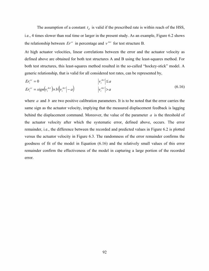
92
The assumption of a constant dt is valid if the prescribed rate is within reach of the HSS,
i.e., 4 times slower than real time or larger in the present study. As an example, Figure 6.2 shows
the relationship between ccEr in percentage and Actv for test structure B.
At high actuator velocities, linear correlations between the error and the actuator velocity as
defined above are obtained for both test structures A and B using the least-squares method. For
both test structures, this least-squares method resulted in the so-called “hockey-stick” model. A
generic relationship, that is valid for all considered test rates, can be represented by,
( ) ( ) avavbvsignEr
avErActi
Acti
Acti
cci
Acti
cci
>−×=
≤= 0 (6.16)
where a and b are two positive calibration parameters. It is to be noted that the error carries the
same sign as the actuator velocity, implying that the measured displacement feedback is lagging
behind the displacement command. Moreover, the value of the parameter a is the threshold of
the actuator velocity after which the systematic error, defined above, occurs. The error
remainder, i.e., the difference between the recorded and predicted values in Figure 6.2 is plotted
versus the actuator velocity in Figure 6.3. The randomness of the error remainder confirms the
goodness of fit of the model in Equation (6.16) and the relatively small values of this error
remainder confirm the effectiveness of the model in capturing a large portion of the recorded
error.

93
-127 -63.5 0 63.5 127Actuator velocity, [mm/sec]
-5 -2.5 0 2.5 5-1
-0.5
0
0.5
1
Actuator velocity, [in/sec]
Erro
r val
ue [%
]
RecordedPredicted
Actv
Actv-127 -63.5 0 63.5 127
Actuator velocity, [mm/sec]
-5 -2.5 0 2.5 5-1
-0.5
0
0.5
1
Actuator velocity, [in/sec]
Erro
r val
ue [%
]
RecordedPredicted
Actv
Actv
Fig. 6.2 Correlation relationship between error cciEr and actuator velocity for test
structure B.
6.2.3 Feed-Forward Error Compensation
Based on the above error relationship with the actuator velocity after calibrating its parameters,
and noting that Activ can be calculated before applying c
id , an error compensation scheme is
devised to eliminate the predicted error. This error compensation is based on adding the
predicted error to the command signal to obtain an adjusted command signal. Subsequently, this
adjusted command signal aid is sent to the actuator in lieu of c
id , where
( ) ( )[ ]( ) av
tdbavsigntddbdd
avdd
Acti
d
Actid
ai
cia
i
Acti
ci
ai
>−
×+−=
≤=
−max
1max
1 (6.17)

94
-5 -2.5 0 2.5 5-0.2
-0.1
0
0.1
0.2
Actuator velocity [in/sec]
Erro
r val
ue [%
]
-127 -63.5 0 63.5 127Actuator velocity [mm/sec]Actv
Actv-5 -2.5 0 2.5 5
-0.2
-0.1
0
0.1
0.2
Actuator velocity [in/sec]
Erro
r val
ue [%
]
-127 -63.5 0 63.5 127Actuator velocity [mm/sec]Actv
Actv
Fig. 6.3 Error remainder (difference between recorded and predicted error values) for test structure B.
This modified command signal aims at the execution of the desired command cid with a
much smaller error caiEr than aa
iEr , where caiEr is the error in c
id when aid is applied and aa
iEr
is the error in aid when a
id is applied analogous to cciEr when error compensation is not
accounted for. An online estimation procedure of the parameters a and b may be developed by
continuously updating the estimates of these parameters during the HS run as the test progresses.
These estimates may be based on an adequate number, to be defined according to the nature of
each HS experiment, of the most recently implemented integration time steps, analogous to the
practical approach in estimating the secant stiffness in FC that is discussed later in Section 6.5.1.
Such a procedure would allow the error prediction and compensation to be implemented during
the same test run thus eliminating the impractical need for a separate run for the purpose of
calibration of the error prediction model and would also make the procedure suitable for
situations where these calibration parameters may change during testing. This is an important
endeavor to be pursued in future enhancements of the develop HSS. The implementation and test
results, validating the developed procedure of the feed-forward error compensation within the
HSS on test structures A and B, are presented in Chapter 7.

95
6.3 MIXED-VARIABLES CONTROL IN HS
While almost all available numerical-integration algorithms implemented in HS solve the
governing equations of motion to yield displacement commands, the idea of solving for force
instead of displacement and conducting the test in FC is an attractive one when considering stiff
structural systems (Thewalt and Mahin 1987). From a computational point of view, analysis
based on a displacement method for structures incorporating flexible and stiff structural elements
may suffer from ill-conditioning of the governing equilibrium equations. Physical modeling of
multiple components (substructures) in a hybrid structural system with different stiffness
properties faces the same difficulties in the conventional pseudo-dynamic testing, with the added
effect of the associated experimental errors. If run in DC, the displacement command values
applied on such systems with high stiffness states would be very small compared to the
resolution of the measuring devices and experimental errors that threaten the accuracy and
stability of the involved numerical integration in the HS. On the other hand, for a certain value of
displacement increment at a given time step, the corresponding restoring-force increment from
such stiff systems is considerably large. Therefore, from the control point of view, these force
increments are more accurate to implement and control than their corresponding small
displacement increments.
It is plausible to envision a situation that requires the use of both control methods, i.e., the
conventional DC and a newly developed FC. For example, in testing systems with bilinear
stiffening behavior, DC may be employed in the flexible state (lower stiffness) and FC in the
stiff state (higher stiffness). In the case of a hybrid structural system, where some substructures
exhibit stiff behavior, while the other substructures exhibit flexible behavior, a mixed-variables
formulation is needed. The governing equations of motion are solved for displacement for the
DOF representing the flexible substructures and solved for force for the DOF representing the
stiff substructures. This leads to a set of mixed variables (forces and displacements) that can be
applied on the respective substructures. The use of mixed-variables “diakoptics” (Kron 1963 and
Wiberg 1974) may alleviate some of the difficulties encountered in testing such hybrid systems
by minimizing the experimental errors and the ill-conditioning of the governing equilibrium
equations. The procedure presented in this chapter offers the possibility of conducting the online
test in any of the two control modes, force or displacement, and switching back and forth
between these modes based on the variation of the state of the DOF in question.

96
6.3.1 FC Integration Algorithm
An integration algorithm with a mixed formulation between force and displacement is
formulated departing from the implicit α -method. First, the implicit FC algorithm is derived.
Second, variation is made to obtain the mixed formulation algorithm. Starting from the equations
of motion defined by Equations (6.1)–(6.7), the following equivalent problem can be formulated,
( ) *111
* 1 +++ =++ iji
ji PRuK α (6.18)
where *K and *1+iP are defined as follows:
( )βγα
β tt Δ++
Δ= CMK 1
2*
(6.19)
( ) ( ) iiiiiii RuKuCuCPPP ααααα ++++−−+= ++++ 1*
11*
1~~11 (6.20)
Considering an iterative solution based on an implicit numerical-integration algorithm,
the displacement at integration time step 1+i and iteration j is stated as follows:
[ ] ( )iji
jii
jii
ji RRKuuuu −+=Δ+= +
−+++ 1
1111 (6.21)
where ji 1+K is the estimated secant stiffness matrix at integration time step 1+i and iteration j ,
with lastii KK =+
11 where last
iK is the estimate of the secant stiffness in the previous ( thi ) time step
at the last iteration. This estimation is iteratively acquired such that the secant stiffness ji 1k + for
every degree of freedom is expressed as follows:
( ) ( )iji
ji
ji uuRRk 1
1i111 −−= −
+−++ (6.22)
The individual stiffness terms for all DOF are then assembled in the stiffness matrix ji 1+K . Note that Equation (6.22) is valid only for physical substructures with a diagonal stiffness
matrix, i.e., systems that may be represented as in parts (A) or (C) in Figure 6.4, where the
linking springs ...,2,1, =ikCi in part (C) are numerically simulated, similar to test structure A.
For systems as in part (B) of Figure 6.4, the computation of the stiffness matrix is possible,
making use of Equation (6.22), but involves solving simultaneous equations. Systems as in part
(D), where the linking springs ...,2,1, =ikPi are modeled physically, are not suited for

97
estimating the stiffness matrix using the simple approach expressed in the above equation (Eq.
6.22) and are out of the scope of this study.
nk
1k
2k1u
2u
nu
1k nk
1u 2u nu
2k
C1k C2k
1k nk
1u 2u nu
2k
P1k P2k
1k 2k nk
1u 2u nu( )A ( )B
( )C ( )D
nk
1k
2k1u
2u
nu
1k nk
1u 2u nu
2k
C1k C2k
1k nk
1u 2u nu
2k
P1k P2k
1k 2k nk
1u 2u nu( )A ( )B
( )C ( )D
Fig. 6.4 Different lumped spring–mass systems.
Rewriting Equation (6.18) using Equation (6.21) one obtains
[ ] ( ){ } [ ] iijii
ji
ji uKRKKPRIKK *1
1**
111
1* 1 −+=++ −
+++−
+ α (6.23)
where I is the identity matrix. From Equation (6.23), the restoring-force vector is obtained and
applied to the test structure under FC. The above algorithm is illustrated in Figure 6.5 where maxi
and maxj are the maximum number of time steps and iterations, respectively, and other
parameters are previously defined in Section 6.1 and Equations (6.18)–(6.23). The stiffness
matrix is updated at the end of each iteration within the integration time step using the last
acquired values of restoring forces R and displacements u and assembled as discussed earlier
with reference to Figure 6.4. The estimation of the components of the stiffness matrix
corresponding to the physical substructures is discussed in details in Section 6.5.1. The tolerance
to be checked for convergence of the iterative solution Rε is expressed in terms of the change of
the restoring force, i.e., the condition for convergence is that for each degree of freedom
Rji
ji ε≤− +
++ 1
11 RR , where Rε is determined based on the resolution of the load cells connected to
the actuators. The higher the number of implemented iterations, the better the chance of
satisfying the convergence tolerance Rε . However, a maximum allowed number of iterations

98
maxj is specified for practical reasons and to prevent the HS system from iterating within the
same numerical-integration time step indefinitely. Note that a practical iterative procedure is
developed in Section 6.5.3 to avoid subjecting the physical substructure to unrealistic
loading/unloading cycles that might be dictated by the implicit FC integration algorithm.
6.3.2 Extension to Mixed-Variables Control
The same integration algorithm in FC can be extended to mixed variables by allocating flexible
DOF to DC and stiff DOF to FC and proceeding as shown in Figure 6.6. Notice that the DC
integration algorithm implemented in the flowchart is the implicit α -method as presented by
Shing et al. (1991). The stiffness matrix is updated at the end of each iteration within the
integration time step for the whole test structure using the same approach discussed in Section
6.3.1. The implicit approach in both DC and FC ensures that equilibrium is satisfied for the
whole test structure, i.e., physical and numerical substructures in DC as well as physical
substructures in FC, at the end of each integration time step. Equilibrium in this case is
represented by Equation (6.23) and is satisfied within acceptable accuracy once the difference
between 21
++jiR and 1
1++jiR is less than the specified tolerance Rε .
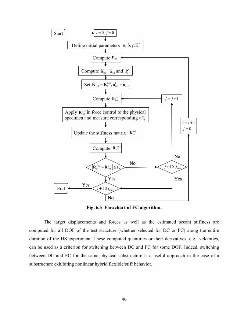
99
Compute 1+iP
Compute , and1~
+iu 1~
+iu *1+iP
Start 0,0 == ji
1+= jjCompute 11
++jiR
Apply in force control to the physicalspecimen and measure corresponding
11
++jiR
11
++jiu
Update the stiffness matrix 11
++jiK
Compute 21
++jiR
01
=+=
jii
Rji
ji ε≤− +
+++
11
21 RR
End
No
Yes
max1 ii ≥+
No
Yes
max1 jj ≥+
Yes
No
Define initial parameters *Kγ,β,α,
Set 11
11
1~=,= +++ ii
lastii uuKK
Compute 1+iPCompute 1+iP
Compute , and1~
+iu 1~
+iu *1+iP
Start 0,0 == ji
1+= jjCompute 11
++jiR
Apply in force control to the physicalspecimen and measure corresponding
11
++jiR
11
++jiu
Update the stiffness matrix 11
++jiK
Compute 21
++jiR
01
=+=
jii
Rji
ji ε≤− +
+++
11
21 RR
End
No
Yes
max1 ii ≥+
No
Yes
max1 jj ≥+
Yes
No
Define initial parameters *Kγ,β,α,
Set 11
11
1~=,= +++ ii
lastii uuKK
Fig. 6.5 Flowchart of FC algorithm.
The target displacements and forces as well as the estimated secant stiffness are
computed for all DOF of the test structure (whether selected for DC or FC) along the entire
duration of the HS experiment. These computed quantities or their derivatives, e.g., velocities,
can be used as a criterion for switching between DC and FC for some DOF. Indeed, switching
between DC and FC for the same physical substructure is a useful approach in the case of a
substructure exhibiting nonlinear hybrid flexible/stiff behavior.

100
Compute 1+iP
Compute , and1~
+iu 1~
+iu *1+iP
Start 0,0 == ji
1+= jj
Compute 11
++jiR
Apply for DOF in FCand measure the
corresponding
11
++jiR
11
++jiu
Update the stiffness matrix 11
++jiK
Compute 21
++
jiR
01
=+=
jii
Rji
ji ε≤− +
+++
11
21 RR
End
No
Yes
max1 ii ≥+
No
Yes
max1 jj ≥+
Yes
No
Define initial parameters *Kγ,β,α,
Set 11
11
1~=,= +++ ii
lastii uuKK
Apply for DOF in DCand determine corresponding forphysical and numerical substructures
11
++jiR
11
++jiu
Compute if11
++jiu 0>j
Compute 1+iPCompute 1+iP
Compute , and1~
+iu 1~
+iu *1+iP
Start 0,0 == ji
1+= jj
Compute 11
++jiR
Apply for DOF in FCand measure the
corresponding
11
++jiR
11
++jiu
Update the stiffness matrix 11
++jiK
Compute 21
++
jiR
01
=+=
jii
Rji
ji ε≤− +
+++
11
21 RR
End
No
Yes
max1 ii ≥+
No
Yes
max1 jj ≥+
Yes
No
Define initial parameters *Kγ,β,α,
Set 11
11
1~=,= +++ ii
lastii uuKK
Apply for DOF in DCand determine corresponding forphysical and numerical substructures
11
++jiR
11
++jiu
Compute if11
++jiu 0>j
Fig. 6.6 Flowchart for integration algorithm with mixed-variables control without mode
switch (DC for flexible DOF and FC for stiff DOF).
The flowchart in Figure 6.7 illustrates the implementation of the integration algorithm
with mode switch between DC and FC for a SDOF system, where maxl and maxj are the
maximum number of iterations in DC and FC, respectively. Note that the DC numerical-
integration algorithm in Figure 6.7 is chosen as the α -method with an operator-splitting scheme
with multiple iterations within the time step, as described in Section 6.1, where the difference
between 21
++
liu and 1
1++
liu needs to satisfy a prescribed tolerance uε , analogous to Rε in FC.

101
Compute 1+iP
Compute , and1~
+iu 1~
+iu *1+iP
Start 0,0,0 === jli
1+= jjCompute 11
++jiR
Apply in FCmeasure corresponding
11
++jiR
11
++jiu
Update the stiffness 11++jik
Compute 21
++jiR
00
1
==
+=
jl
ii
Rji
ji ε≤− +
+++
11
21 RR
End
NoYes
max1 ii ≥+
No
Yes
max1 jj ≥+
Yes
No
Define initial parameters MK ˆ,γ,β,α, *
Set 11
11
1~=,= +++ ii
lastii kk uu
Apply in DC measure corresponding 1
1~ +
+liR
Compute , 11
111
ˆˆ= ++
−++
li
li PMu1
1ˆ +
+l
iP
Compute corrected 11
++
liu
DC Control mode ? FC
Update the stiffness 11
++lik
Set 11
1~= ++ ii uu
11
++
liu
1+= ll
Compute 21
++
liu
uli
li ε≤− +
+++
11
21 uu Yes
max1 ll ≥+
Yes
NoNo
Fig. 6.7 Flowchart for integration algorithm with mode switch between DC and FC for SDOF system.
However, other DC numerical-integration algorithms may be used as long as equilibrium
is satisfied at the end of each integration time step, as discussed in Section 6.1 for the selected
DC integration algorithm. The stiffness matrix is updated at the end of each iteration within the
integration time step for the whole test structure using the same approach discussed in Section
6.3.1, and the decision to switch between the two control modes is discussed in details in Section
6.5.2. Note that selecting DOF for pure DC and others for DC with the possibility of switching to
FC and back, according to the state of the test structure, is possible by using the algorithm shown
in Figure 6.6 and adopting for each degree of freedom, having the possibility of mode switch, the
algorithm shown in Figure 6.7.
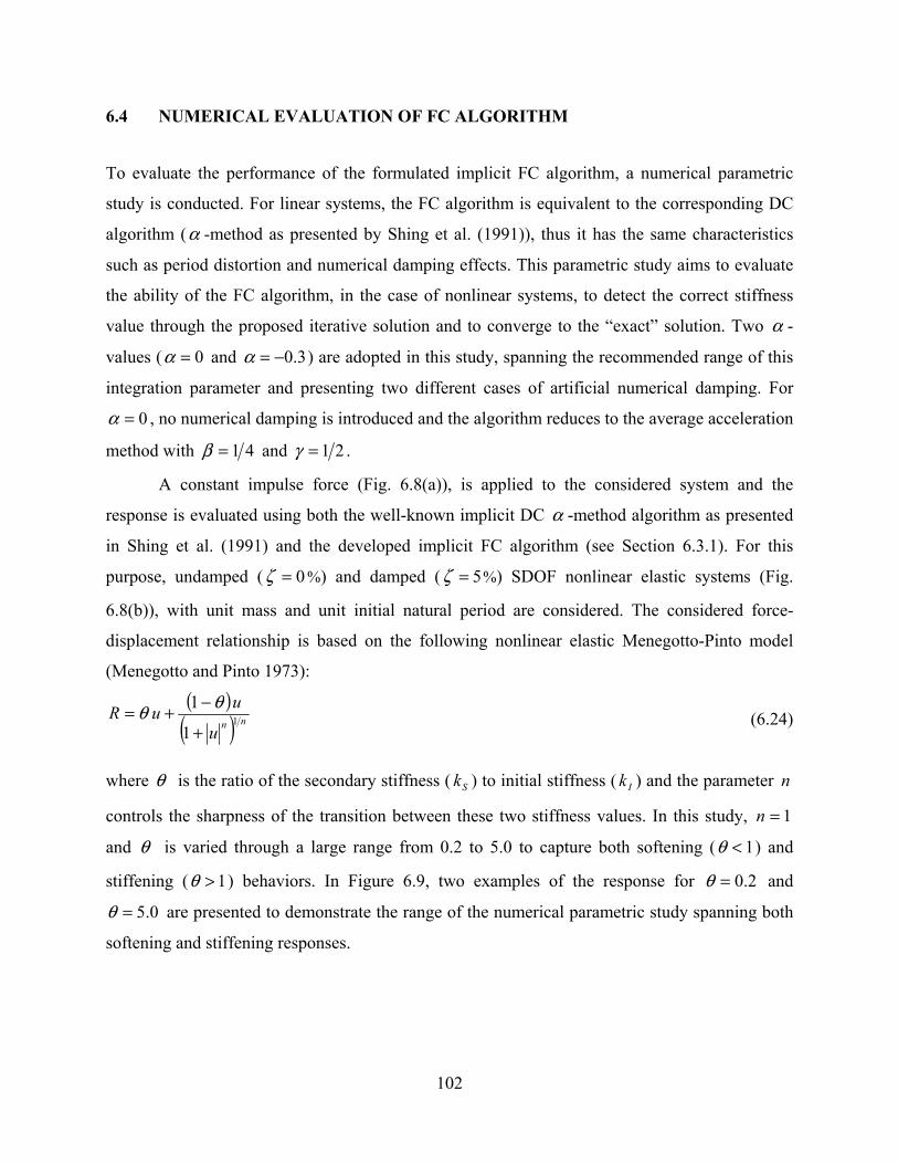
102
6.4 NUMERICAL EVALUATION OF FC ALGORITHM
To evaluate the performance of the formulated implicit FC algorithm, a numerical parametric
study is conducted. For linear systems, the FC algorithm is equivalent to the corresponding DC
algorithm (α -method as presented by Shing et al. (1991)), thus it has the same characteristics
such as period distortion and numerical damping effects. This parametric study aims to evaluate
the ability of the FC algorithm, in the case of nonlinear systems, to detect the correct stiffness
value through the proposed iterative solution and to converge to the “exact” solution. Two α -
values ( 0=α and 3.0−=α ) are adopted in this study, spanning the recommended range of this
integration parameter and presenting two different cases of artificial numerical damping. For
0=α , no numerical damping is introduced and the algorithm reduces to the average acceleration
method with 41=β and 21=γ .
A constant impulse force (Fig. 6.8(a)), is applied to the considered system and the
response is evaluated using both the well-known implicit DC α -method algorithm as presented
in Shing et al. (1991) and the developed implicit FC algorithm (see Section 6.3.1). For this
purpose, undamped ( 0=ζ %) and damped ( 5=ζ %) SDOF nonlinear elastic systems (Fig.
6.8(b)), with unit mass and unit initial natural period are considered. The considered force-
displacement relationship is based on the following nonlinear elastic Menegotto-Pinto model
(Menegotto and Pinto 1973):
( )( ) nnu
uuR 11
1
+
−+= θθ (6.24)
where θ is the ratio of the secondary stiffness ( Sk ) to initial stiffness ( Ik ) and the parameter n
controls the sharpness of the transition between these two stiffness values. In this study, 1=n
and θ is varied through a large range from 0.2 to 5.0 to capture both softening ( 1<θ ) and
stiffening ( 1>θ ) behaviors. In Figure 6.9, two examples of the response for 2.0=θ and
0.5=θ are presented to demonstrate the range of the numerical parametric study spanning both
softening and stiffening responses.

103
0 0.5 10
1
2
Time
App
lied
forc
e
k
umζ
k
umζ
(a) Applied constant impulse force (b) Considered system
Fig. 6.8 Applied force and considered system for numerical evaluation of FC algorithm.
∞atSk
Ik at origin
Res
torin
g fo
rce,
R
uDisplacement,
∞atSk
Ik at origin
Res
torin
g fo
rce,
R
uDisplacement, uDisplacement,
Ik at origin
∞atSk
uDisplacement,
Res
torin
g fo
rce,
R
Ik at origin
∞atSk
uDisplacement, uDisplacement,
Res
torin
g fo
rce,
R
(a) 2.0=θ (b) 0.5=θ
Fig. 6.9 Nonlinear elastic response using Menegotto-Pinto model ( IS kk =θ ).
To evaluate the deviation of the numerical solution from the exact solution, the following
error quantity is defined for the considered cases,
[ ] 100% ×−
=∑
∑
i
Exacti
i
Exacti
gAli
gAl
S
SSEr (6.25)
where ( ) ( ) 2111 −−− +×++= iiiiii uuRRSS is the strain energy at time step i , and iR and iu are the
restoring force and displacement at time step i , respectively. The superscripts gAl and Exact
refer to the response of the algorithm in question and the exact response, respectively. This exact

104
response is the converged solution obtained using the implicit average acceleration method with
a very small integration time step, namely 5102 −×=Δt sec. The secant stiffness is calculated
numerically as in Equation (6.22), the convergence tolerances for displacement and force are 1010−== Ru εε , respectively, with a maximum of 10 iterations, where Rε and uε are defined in
Section 6.3.1 and 6.3.2, respectively. Eight cases are studied (Table 6.1) for each of the two
integration algorithms resulting from the eight possible different combinations of the three varied
parameters, α , ζ , and tΔ . Figure 6.10 shows two identical curves (solid for FC and dashed for
DC), for each of the eight studied cases, designating the calculated responses using the implicit
FC method and the DC method, thus confirming the ability of the new FC algorithm to produce
as accurate a solution as the DC algorithm. Note that the estimated error values increase with the
increase of θ , plotted on the x-axis in a logarithmic scale, due to the decrease of the natural
period of the studied system, while the integration time step tΔ is kept constant. For a smaller
tΔ for the same considered system, the error significantly decreases as expected. The level of
variation in the estimated error is much higher in the case of 02.0=Δt sec, implying that the
ratio tT Δ reaches levels where the accuracy of the numerical-integration algorithm is affected
significantly, when compared to the case of 005.0=Δt sec.
Table 6.1 Varied parameters for numerical evaluation of FC algorithm.
Integration
parameter
Damping
ratio
Integration
time step
0=α %0=ζ 02.0=Δt sec
3.0−=α %5=ζ 005.0=Δt sec

105
10-1
100
101
0
5
10
15
20
Erro
r val
ue, E
rAlg [%
]
FCDC
10-1
100
101
0
5
10
15
20
Erro
r val
ue, E
rAlg [%
]
FCDC
θ θ
3.0−=α0=α
005.0=Δt
02.0=Δt %5=ζ
%0=ζ
%5=ζ
%0=ζ
%0=ζ
%5=ζ%0=ζ
%5=ζ
005.0=Δt
02.0=Δt
10-1
100
101
0
5
10
15
20
Erro
r val
ue, E
rAlg [%
]
FCDC
10-1
100
101
0
5
10
15
20
Erro
r val
ue, E
rAlg [%
]
FCDC
θ θ
3.0−=α0=α
005.0=Δt
02.0=Δt %5=ζ
%0=ζ
%5=ζ
%0=ζ
%0=ζ
%5=ζ%0=ζ
%5=ζ
005.0=Δt
02.0=Δt
Fig. 6.10 Parametric study of FC and DC algorithms using nonlinear elastic SDOF systems.
6.5 IMPLEMENTATION STRATEGIES OF MIXED-VARIABLES CONTROL
The different operations and strategies needed for the implementation of the mixed-variables HS
procedure are presented in this section. This includes the procedure of stiffness estimation,
criteria, and decisions on control mode switching between force and displacement and a practical
iterative approach to avoid unrealistic loading and unloading cycles.
6.5.1 Secant Stiffness Estimation
The developed FC algorithm relies on the estimation of the secant stiffness during the HS
experiment at the end of each iteration within the integration time step. The most direct way of
estimating the stiffness is by using the displacement and force feedback signals at the end of each
iteration using Equation (6.22). However, the resolutions of the measuring sensors for force and
displacement in addition to the random noise associated with the feedback signals can

106
considerably affect this estimation. A procedure is therefore developed to minimize these effects
and to obtain an improved accuracy in estimating the secant stiffness. Noting that the feedback
signals are available at a very high frequency in the xPC target (1024 Hz) through ScramNet (see
Section 3.3), average values over the last AvgN feedbacks in one iteration within the time step
for each of the quantities in Equation (6.22) are used instead, e.g., in the application example
discussed in Chapter 7 with sec2=dt , TR =400, and sec005.0=Δt , AvgN is taken as 100 out of
dt1024 = 2048 points, i.e., by averaging the last 5% of the available feedbacks in one iteration
within the time step. Subsequently, the averaged signals are passed to the numerical-integration
algorithm in the MATLAB environment to calculate an average stiffness ( )Avgjik 1+ for each
degree of freedom (Fig. 6.11). These average stiffness are subsequently assembled into the
stiffness matrix ( )Avgji
1+K with the limitations discussed in reference to Figure 6.4. Figure 6.12
shows a more reliable ( )Avgi 1+K when compared to 1+iK , using the displacement and force
feedback signals at the end of each iteration, for a representative HS of test structure B. Although
yielding similar values in most of the shown plot, where the restoring force R and the
displacement increments become smaller at the peaks of a loading cycle, an unrealistic large
negative stiffness K is estimated, while AvgK does not suffer from this anomalous fluctuation.
Note that for faster rates, where the time-step duration decreases and the available number of
feedback signals in the xPC target within one iteration decreases, if AvgN needs to be reduced to
the point where the averaging effect would be lost, other techniques may be implemented such as
the least-squares method to evaluate a linear secant stiffness over the whole integration time step.

107
AvgiR
( )AvgjiR 1
1−
+
5
1
7
1
7
.5
1
8
1
8
.5
1
9
11−
+j
iu
11−
+j
iR
iu
iR
Avgiu ( )Avgj
iu 11−
+
AvgN
AvgN
( )Avgjik 1+
jik 1+
AvgiR
( )AvgjiR 1
1−
+
5
1
7
1
7
.5
1
8
1
8
.5
1
9
11−
+j
iu
11−
+j
iR
iu
iR
Avgiu ( )Avgj
iu 11−
+
AvgN
AvgN
( )Avgjik 1+
jik 1+
Fig. 6.11 Schematic representation of secant stiffness estimation at time step i +1 and iteration j .
900 950 1000-200
-100
0
100
200
Time step
Ku
AvgK(35.0)
(-17.5)
Mea
sure
d sti
ffnes
s [ki
p/in
(kN
/mm
)]
4(100.8)
2(50.4)
0
(-50.4) -2
(-100.8)-4
Mea
sure
d di
spla
cem
ent [
in (m
m)]
(17.5)
(-35.0)
900 950 1000-200
-100
0
100
200
Time step
Ku
AvgK(35.0)
(-17.5)
Mea
sure
d sti
ffnes
s [ki
p/in
(kN
/mm
)]
4(100.8)
2(50.4)
0
(-50.4) -2
(-100.8)-4
Mea
sure
d di
spla
cem
ent [
in (m
m)]
(17.5)
(-35.0)
900 950 1000-200
-100
0
100
200
Time step
KR
AvgK(35.0)
(-17.5)
Mea
sure
d sti
ffnes
s [ki
p/in
(kN
/mm
)]
10(44.4)
5(22.2)
0
(-22.2) -5
(-44.4)-10
Mea
sure
d fo
rce
[kip
(kN
)]
(17.5)
(-35.0)
900 950 1000-200
-100
0
100
200
Time step
KR
AvgK(35.0)
(-17.5)
Mea
sure
d sti
ffnes
s [ki
p/in
(kN
/mm
)]
10(44.4)
5(22.2)
0
(-22.2) -5
(-44.4)-10
Mea
sure
d fo
rce
[kip
(kN
)]
(17.5)
(-35.0)
(a) Loading/unloading cycle showing displacement history
(b) Loading/unloading cycle showing restoring-force history
Fig. 6.12 Example results from test structure B for estimation of secant stiffness.

108
6.5.2 Mode-Switch Decision Implementation
There are constraints on the use of FC, which are different in nature than in DC. For instance, if
the substructure approaches its ultimate load-carrying capacity during the HS experiment, the
force command may exceed that capacity and the control system may drive the test structure to
failure. Therefore, switching criteria are needed to carefully decide on the control mode, in
which any integration time step i will be executed, for the DOF in question. These criteria are
adopted based on the knowledge of the behavior of the test structure, such as applying tension or
compression load as in Pan (2004) and Pan et al. (2005). Both DC and FC integration algorithms
are performed in parallel during the full time history, as described in Section 6.3.2, and at the end
of each time step, a decision is made whether to stay in the current control mode (e.g., DC) or to
switch to the other control mode (e.g., FC). Figure 6.12 shows the decision-making scheme
implemented using as an example two criteria for switching, namely the secant stiffness K and
the restoring force R with estimated values iK and iR at the i -th time step, respectively. Two
threshold values are needed for each switching criterion, e.g., dK and fK for K , where
fd KK < . This provides a buffer zone to avoid switching back and forth between the two control
modes in the case where the measured AvgK fluctuates slightly in the range of these threshold
values. The threshold values are determined based on the expected fluctuations of the estimated
quantity they are being compared to, e.g., a minimum difference between dK and fK would be
the resolution at which AvgK is estimated, plus a certain margin of fluctuation. In the present
study, this margin was estimated by monitoring AvgK in the regions where mode switching is
expected to take place from past experiences. An example for the evaluation of these thresholds
in the case of test structure B is discussed in Chapter 7.

109
Start Calculate ii R,K
Current mode?
fi KK >fi RR > Displacement
Force
Yes YesSwitch to forcecontrol mode
Stay at current mode
NoSwitch to displacementcontrol Mode
End
No
No No
Yes Yes
Define thresholdsand
fdfd R,R,K,Kfd KK < fd RR <
di KK <di RR <
Start Calculate ii R,K
Current mode?
fi KK >fi RR > Displacement
Force
Yes YesSwitch to forcecontrol mode
Stay at current mode
NoSwitch to displacementcontrol Mode
End
No
No No
Yes Yes
Define thresholdsand
fdfd R,R,K,Kfd KK < fd RR <
di KK <di RR <
Fig. 6.13 Mode-switch decision-making scheme.
Once the decision is made to switch between control modes, the STS controller needs to
switch to that mode and to execute the corresponding command signal. In the present study, this
is accomplished by having the control mode as an additional Boolean command conveyed by
Simulink to STS along with the displacement and force command signals (see Fig. 3.2). This
feature was incorporated into the HSS to accommodate the possibility of conducting HS
experiments with control mode switch1. It is worth mentioning that the
extrapolation/interpolation implementation strategy is not suitable for an implicit algorithm
where iterations are required as discussed in Section 3.5. This feature is therefore turned off
when the implicit mixed-variables algorithm with mode-switching capabilities is invoked and a
linear interpolation, from the current state to the new command, is implemented instead.
At the end of the integration time step i , if mode switch is decided to take place in step
i +1, e.g., from DC to FC, the actuator is locked at the current displacement lastiu , which is the
calculated target displacement command by the DC integration algorithm at the last iteration of
time step i . Next, the control mode switch takes place and the actuator is locked at the current
force command lastiR , which is the last restoring-force feedback in time step i corresponding to
lastiu , i.e., maintaining and starting from an equilibrium state. The actuator is ready at this point to
implement the next target force 11+iR calculated iteratively by the FC integration algorithm.
1 The authors would like to acknowledge the collaboration of MTS in adding the mode switch feature to the hybrid controller at nees@berkeley

110
6.5.3 Practical Iterative Solution
The developed mixed-variables algorithm (for DC and FC, see Fig. 6.7) is implicit and thus
requires iterations. However, the loading and unloading of a nonlinear inelastic system may
cause unrealistic loading/unloading cycles and subsequently a distortion of the calculated secant
stiffness. From Equation (6.23), we note that the only implicit term in calculating 11
++jiR is 1
1++jiK .
This secant stiffness may be estimated by applying a fraction of the increment ji
ji 1
11 +
++ − RR at
each time step until convergence is reached, thus avoiding the unrealistic loading/unloading
cycles. Therefore, instead of applying the full increment, as implied by the algorithm in Figures
6.5–6.7, only a fraction ( )ji
ji 1
11 +
++ − RRλ is applied for each iteration, where 1<λ , and 1
1++jiK is
estimated until the tolerance Rε (Fig. 6.5) is satisfied and finally the remaining of lasti 1+R , which is
the calculated force command by the integration algorithm in the last iteration is fully
implemented on the test structure.
To evaluate the effect of this iterative implementation strategy including the mode-switch
decision-making scheme, a stiffening bilinear elastic SDOF undamped system (Fig, 6.14) with
similar properties to that used in the previous parametric study, discussed in Section 6.4, is
selected and subjected to the same impulse force (see Fig. 6.8(a)). Displacement control with an
operator-splitting scheme and one predictor-corrector cycle, discussed in Section 6.1, is used
during the initial (smaller) stiffness, Ik , while FC is used during the (higher) secondary stiffness,
Sk , for ( 1>= IS kkθ ). Four cases are studied (Table 6.2) resulting from the four possible
different combinations of the two varied parameters, α and tΔ .
5
Ik
Sk
uDisplacement,
Res
torin
g fo
rce,
R
5
Ik
Sk
uDisplacement, uDisplacement,
Res
torin
g fo
rce,
R
Fig. 6.14 Considered stiffening bilinear elastic system for numerical evaluation.

111
The strain energy error in the present parametric study is calculated from Equation (6.25)
based on a closed-form solution of the dynamic problem, Appendix B. The shown numerical
solutions labeled “MS,” i.e., mode switch, in Figure 6.15 correspond to 2max =j , and 0=Rε ,
i.e., two iterations are always carried out. Moreover, 5.0=λ is selected in the present numerical
parametric study. These parameters are selected to simulate the case of a HS experiment with a
limited number of iterations applied within each integration time step. In the DC solution (Fig.
6.15), the DC integration algorithm with one predictor-corrector cycle, discussed in Section 6.1,
is used for the entire length of the applied motion without mode switch for the purpose of
comparison with the mode switch (MS) curves. While in the case of 02.0=Δt sec, the DC
solution is more accurate, in the case of 005.0=Δt sec, the two approaches yield almost
identical error values indicating the accuracy of this solution if an adequate tΔ is used. Note that
the same increase of the error values with the increase in θ observed in Figure 6.10 is observed
in this numerical study as well. The higher error values for the case where 3.0−=α are due to
the exact solution, with respect to which the error is calculated. As this solution is in closed form,
the numerical dissipation introduced by the non-zero value of α , leads to an additional source of
error.
1 2 3 4 50
5
10
15
Ener
gy E
rror [
%]
MSDC
1 2 3 4 50
5
10
15
Ener
gy E
rror [
%]
MSDC
θ θ
3.0−=α0=α
005.0=Δt
02.0=Δt
005.0=Δt
02.0=Δt
Erro
r val
ue, E
rAlg [%
]
Erro
r val
ue, E
rAlg [%
]
1 2 3 4 50
5
10
15
Ener
gy E
rror [
%]
MSDC
1 2 3 4 50
5
10
15
Ener
gy E
rror [
%]
MSDC
θ θ
3.0−=α0=α
005.0=Δt
02.0=Δt
005.0=Δt
02.0=Δt
Erro
r val
ue, E
rAlg [%
]
Erro
r val
ue, E
rAlg [%
]
Fig. 6.15 Parametric study of mode-switch algorithm using bilinear elastic SDOF systems.

112
Table 6.2 Varied parameters for numerical evaluation of mode-switch and iterative approach.
Integration parameter Integration time step
0=α and 3.0− 02.0=Δt and 0.005 sec
6.6 SUMMARY
The present study uses the α -method (Hilber et al. 1977) as presented by Shing et al. (1991)
along with the operator splitting scheme (Nakashima 1990) to solve the governing equations of
motion and to perform the experiments in displacement control. This numerical-integration
algorithm is presented in detail. Two procedures are developed and implemented in the hybrid
simulation system with the aim of enhancing the accuracy and reliability of the pseudo-dynamic
test results. The first procedure aims at correcting the experimental systematic error in executing
the displacement command signal. The error is calculated as the difference between command
and feedback signals and correlated with the actuator velocity using a “hockey-stick” model. A
feed-forward scheme for error compensation is devised leading to a more accurate execution of
the hybrid simulation experiment. The second procedure employs mixed-variables with mode
switching between displacement and force controls. The newly derived force-control algorithm is
evaluated using a parametric study to assess its stability and accuracy by comparing its numerical
results to those of the α -method in displacement control. The implementation of the mixed-
variables control procedure is designed to adopt force control for high stiffness states of the
structural response and displacement control otherwise, where the resolution of the involved
instruments may favor this type of mixed control. A number of practical implementation
strategies are developed to support the execution of the new force-control algorithm within the
hybrid simulation system of nees@berkeley.

7 Applications of Developed Hybrid Simulation Procedures
This chapter focuses on presenting results from phases P-1 and P-2 (see Fig. 1.2). The two
developed procedures presented in Chapter 6, namely: (1) feed-forward error compensation and
(2) mixed-variables control are applied on the two test structures, A and B, presented in Chapters
4 and 5, respectively.
7.1 FEED-FORWARD ERROR COMPENSATION
The feed-forward error prediction, presented in Section 6.2.2, is applied on test structures A and
B. For each test structure, the calibration parameters in Equation (6.16) are evaluated using the
least-squares method and used as described in Section 6.2.3 to compensate for these predicted
displacement execution errors.
7.1.1 Calibration Parameter Evaluation
The strong motion LPB level 9 (see Tables 4.1–4.2) is applied on test structure A, while LPG
level 5 (see Tables 5.1–5.2) is applied on test structure B, at varying test rates from 50 to 6.25
times slower than real time. Note that at faster test rates, the inertial force experienced by the
physical substructures is included in the actuator force feedback signal and may be a source of
error in the estimation of the restoring forces. However, the mass of the physical substructures in
test structures A and B constituted ≈ 5% in both cases from the total numerically simulated mass
of the HS test structure. In the case of the fastest test rate applied (6.25 times slower than real
time), the accelerations imposed on the physical substructure are 6.25 2 = 39 times less than the
numerically simulated ones, which was confirmed by the measured accelerations at the RC beam
level of test structure A (see Section 4.5). Therefore, the total inertial force added to the actuator

114
force feedback signal amounts to less than 0.13% of the total numerically simulated inertial force
and is safely neglected. The actuator velocity and the corresponding predicted error at the end of
each integration time step are recorded (see Section 6.2) and plotted in Figure 7.1(a) and (b), for
test structures A and B, respectively, along with their least-squares fits based on the calibrated
parameters. The values of the calibration parameters are presented in Table 7.1.
The two application examples are different in terms of the applied strong motion, the test
structures, and their corresponding structural behaviors, as well as the PIDF tuning control
parameters (see Section 3.4.1). Note that while the same actuators are used in the two
experiments, two different sets of tuning parameters were used as the framework was being
developed and better tuning was achieved in the case of test structure B than that of test structure
A. The parameters a and b are therefore different in value (larger a and smaller b implying
better control for test structure B) but the hockey-stick model described by Equation (6.16) holds
implying its generic applicability in the case of the used HSS. The limitation of this error
compensation procedure is due to the need of evaluating these calibration parameters before the
actual test in a trial run, which may not be possible in all experimental investigations. An online
calibration process for these parameters is a possible way to counter that problem and may be the
subject of future development of the procedure as previously discussed in Section 6.2.3.
Table 7.1 Calibration parameters for feed-forward error compensation procedure, Eq.
6.17.
Calibration parameter a [in./sec (mm/sec)] b [sec/in. (sec/mm)] Test structure A 0.0202 (0.51) 0.0030 (1.18×10⁻⁴) Test structure B 0.2040 (5.18) 0.0021 (7.87×10⁻⁵)

115
-127 -63.5 0 63.5 127
-1
-0.5
0
0.5
1
Actuator velocity, [mm/sec]
-5 -2.5 0 2.5 5-1
-0.5
0
0.5
1
Actuator velocity, [in/sec]
Erro
r val
ue [%
]
RecordedPredicted
Actv
Actv
-127 -63.5 0 63.5 127
-1
-0.5
0
0.5
1
Actuator velocity, [mm/sec]
-5 -2.5 0 2.5 5-1
-0.5
0
0.5
1
Actuator velocity, [in/sec]
Erro
r val
ue [%
]
RecordedPredicted
Actv
Actv
-127 -63.5 0 63.5 127
-1
-0.5
0
0.5
1
Actuator velocity, [mm/sec]
-5 -2.5 0 2.5 5-1
-0.5
0
0.5
1
Actuator velocity, [in/sec]
Erro
r val
ue [%
]
RecordedPredicted
Actv
Actv
-127 -63.5 0 63.5 127
-1
-0.5
0
0.5
1
Actuator velocity, [mm/sec]
-5 -2.5 0 2.5 5-1
-0.5
0
0.5
1
Actuator velocity, [in/sec]
Erro
r val
ue [%
]
RecordedPredicted
Actv
Actv
(a) Test structure A
-127 -63.5 0 63.5 127Actuator velocity, [mm/sec]
-5 -2.5 0 2.5 5-1
-0.5
0
0.5
1
Actuator velocity, [in/sec]
Erro
r val
ue [%
]
RecordedPredicted
Actv
Actv-127 -63.5 0 63.5 127
Actuator velocity, [mm/sec]
-5 -2.5 0 2.5 5-1
-0.5
0
0.5
1
Actuator velocity, [in/sec]
Erro
r val
ue [%
]
RecordedPredicted
Actv
Actv
(b) Test structure B
Fig. 7.1 Correlation relationship between error cciEr and actuator velocity.

116
7.1.2 Experimental Results
The same strong motions described in the previous section are applied on the respective test
structures with the feed-forward error compensation scheme developed in Section 6.2.3. At any
time step i , the adjusted command signal aid is therefore sent to the actuators instead of the
calculated command cid . This modified command aims at the execution of the desired command
cid with a much smaller ca
iEr than aaiEr , where ca
iEr is the error in cid when a
id is applied and
aaiEr is the error in a
id when aid is applied. Figures 7.2(a)–(b) show the results of the
implementation of the feed-forward error compensation procedure on test structure A at a test
rate TR = 40 times slower than real time and on test structure B at TR = 6.25 time slower than
real time, respectively. The error signal caiEr is reduced to a maximum of 0.041% from a
maximum aaiEr of 0.353% in test structure A and 0.104% (excluding one anomalous peak of the
recorded caiEr signal treated as an outlier) from 0.797% in the case of test structure B. In both
cases the reduced error is much closer than the original error to the displacement feedback
resolution level, which is ±0.001 in. (±0.025 mm), i.e., 0.01%. The effectiveness of the feed-
forward error compensation in executing a more accurate displacement command signal, where
the error is reduced to less than 13% of the original error, is therefore confirmed.
7.2 MIXED-VARIABLES CONTROL
The mixed-variables (force/displacement) control procedure with mode switch developed in
Chapter 6 is implemented on test structures A and B following the algorithm illustrated in Figure
6.7. Force control is adopted for stiff states of the response while DC is adopted otherwise, as
discussed in subsequent sections. Note that the developed practical iterative solution strategy
(see Section 6.5.3) was not developed at the time of implementing the mixed-variables control on
test structure A. In addition, the actuator tuning in FC was not adequate enough to ensure an
accurate execution of the force command signal for test structure A which led to a poorly
executed test. The following discussion is therefore limited to test structure B where these two
limitations were overcome, while a brief discussion of the results of test structure A is included
at the end of Section 7.2.3.

117
0 5 10 15-1
-0.5
0
0.5
1
Time [sec]
Erro
r val
ue [%
]
caiEraa
iEr
TR = 40
0 5 10 15-1
-0.5
0
0.5
1
Time [sec]
Erro
r val
ue [%
]
caiEraa
iEr
TR = 40
(a) Test structure A (TR = 40 times slower than real time)
0 5 10 15 20-1
-0.5
0
0.5
1
Time [sec]
Erro
r val
ue [%
]
caiEraa
iEr
TR = 6.25
0 5 10 15 20-1
-0.5
0
0.5
1
Time [sec]
Erro
r val
ue [%
]
caiEraa
iEr
TR = 6.25
(b) Test structure B (TR = 6.25 times slower than real time)
Fig. 7.2 Feed-forward error compensation results.
7.2.1 Structural States
The typical structural behavior exhibited by test structure B is illustrated in Figure 7.3. The wood
structure is characterized by a low loading stiffness (< 3 kip/in. (0.53 kN/mm)) and a much
higher unloading stiffness (> 30 kip/in. (5.3 kN/mm)) in the circled parts of the response in

118
Figure 7.3. At these relatively higher stiffness values, the PIDF control can be used to apply the
command signal in FC mode with better accuracy than in DC mode. Note that in the stiff state,
since the displacement increments are small, the actuator velocity is too small for the feed-
forward error compensation procedure to be effective. Therefore, this error compensation is not
considered in this section.
-5 -2.5 0 2.5 5-10
-5
0
5
10
Displacement [in]
Forc
e [k
ip]
Stiff regions
Displacement [mm]-127 -63.5 0 63.5 127 44.5
22.2
0
-22.2
-44.5
Forc
e [k
N]
-5 -2.5 0 2.5 5-10
-5
0
5
10
Displacement [in]
Forc
e [k
ip]
Stiff regions
Displacement [mm]-127 -63.5 0 63.5 127 44.5
22.2
0
-22.2
-44.5
Forc
e [k
N]
Fig. 7.3 Typical force-deformation response for test structure B.
7.2.2 Mode-Switch Decision Making
The FC actuator tuning (see Section 3.4.1) is stiffness dependent and requires the presence of a
physical specimen to calibrate the PIDF tuning parameters. Accordingly, two shear walls, similar
to the physical substructure in test structure B, are used for that purpose, then removed and
replaced by the physical substructure of test structure B. The current HS setup does not allow the
PIDF tuning parameters to be varied during the test. Therefore, the actuator is tuned in FC for the
higher range of stiffness around 40 kips/in. (7.0 kN/mm). Since the stiffness needs to be in the
tuning range, i.e., neither much higher nor much lower in order to apply the command in FC
accurately, two switching criteria are adopted, both based on the estimated secant stiffness. Each

119
upper and lower secant stiffness limit is defined by two threshold values updK = 65 kips/in. (11.4
kN/mm) and upfK = 60 kips/in. (10.5 kN/mm) for the upper limit and low
fK = 25 kips/in. (4.4
kN/mm) and lowdK = 20 kips/in. (3.5 kN/mm) for the lower limit. Figure 7.4 illustrates the use of
these limits in the mode-switch decision-making procedure (see Section 6.5.2). Notice the two
buffer zones between lowdK and low
fK on one side and between updK and up
fK on the other side of
the figure. These buffer zones prevent the HSS from switching back and forth between the two
control modes in the case where the amplitude of the estimated parameter iK fluctuates slightly
around the value of one of the thresholds. Based on the above thresholds, the mode-switch
decision-making scheme is shown in Figure 7.5. Compared to Figure 6.13, another third criterion
for mode switch is added such that FC is used only in the unloading regions, where
01 <Δ=− − iii RRR . From Figures 7.4–7.5, FC is used in the unloading parts where the estimated
average stiffness lies in the designated range ( upAvglow KKK •• << ), where subscript • denotes d
or f depending on the current control mode, i.e., FC or DC, respectively; otherwise DC is
employed.
Current Mode
FC
FC
DC
DC
DC
FC
lowfKlow
dK upfK up
dKRange of estimated average stiffness and new mode
DC
DC
Current Mode
FC
FC
DC
DC
DC
FC
lowfKlow
dK upfK up
dKRange of estimated average stiffness and new mode
DC
DC
Fig. 7.4 FC/DC mode-switch criteria for application example (test structure B).
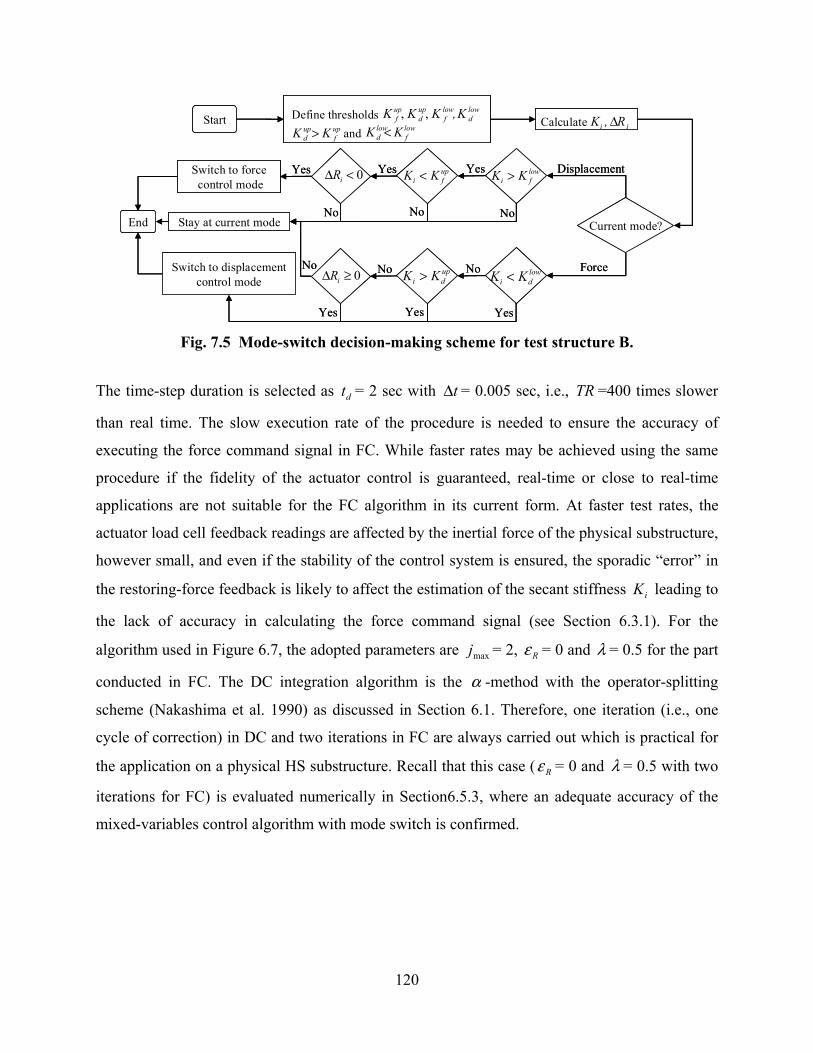
120
Yes Yes
Start Calculate ii R,K Δ
Current mode?
lowfi KK > Displacement
Force
Switch to forcecontrol mode
Stay at current mode
NoSwitch to displacementcontrol mode
EndNo No
Yes Yes
Define thresholdsand
lowd
lowf
upd
upf K,KKK ,,
upf
upd KK > low
flowd KK <
0<Δ iR Yes upfi KK <
No lowdi KK <No up
di KK >
Yes
0≥Δ iR
No
Yes Yes
Start Calculate ii R,K Δ
Current mode?
lowfi KK > Displacement
Force
Switch to forcecontrol mode
Stay at current mode
NoSwitch to displacementcontrol mode
EndNo No
Yes Yes
Define thresholdsand
lowd
lowf
upd
upf K,KKK ,,
upf
upd KK > low
flowd KK <
0<Δ iR Yes upfi KK <
No lowdi KK <No up
di KK >
Yes
0≥Δ iR
No
Fig. 7.5 Mode-switch decision-making scheme for test structure B.
The time-step duration is selected as dt = 2 sec with tΔ = 0.005 sec, i.e., TR =400 times slower
than real time. The slow execution rate of the procedure is needed to ensure the accuracy of
executing the force command signal in FC. While faster rates may be achieved using the same
procedure if the fidelity of the actuator control is guaranteed, real-time or close to real-time
applications are not suitable for the FC algorithm in its current form. At faster test rates, the
actuator load cell feedback readings are affected by the inertial force of the physical substructure,
however small, and even if the stability of the control system is ensured, the sporadic “error” in
the restoring-force feedback is likely to affect the estimation of the secant stiffness iK leading to
the lack of accuracy in calculating the force command signal (see Section 6.3.1). For the
algorithm used in Figure 6.7, the adopted parameters are maxj = 2, Rε = 0 and λ = 0.5 for the part
conducted in FC. The DC integration algorithm is the α -method with the operator-splitting
scheme (Nakashima et al. 1990) as discussed in Section 6.1. Therefore, one iteration (i.e., one
cycle of correction) in DC and two iterations in FC are always carried out which is practical for
the application on a physical HS substructure. Recall that this case ( Rε = 0 and λ = 0.5 with two
iterations for FC) is evaluated numerically in Section6.5.3, where an adequate accuracy of the
mixed-variables control algorithm with mode switch is confirmed.

121
7.2.3 Experimental Results
The procedure discussed above is applied on test structure B using the strong motion LPG level 5
(see Tables 5.1–5.2). Figure 7.6(a) shows part of the implemented history where large
loading/unloading cycles are reported. The dashed red line indicates whether DC or FC is
employed corresponding to zero or non-zero value, respectively. Force control is used in the
unloading parts where the measured stiffness lies in the designated range in Figures 7.4–7.5;
otherwise DC is employed. This is illustrated more clearly in Figure 7.6(b) where an enlarged
part of a cycle is shown. Due to the fast rate of change of stiffness during unloading, two
integration time steps (number 974 and 975) are implemented in FC. Nevertheless, mode switch
within the HSS occurs smoothly between DC and FC and vice versa, without disturbing the
feedback signals of the restoring force or displacement. The estimation of the secant stiffness, as
a result, is reliable for its use in the mixed-variables numerical-integration algorithm. The
execution of the force command signals is highly accurate as demonstrated by the measured
feedback restoring-force signals, mR in Figure 7.6(b), which match the corresponding command
signals within the resolution of the measuring sensor, i.e., ±0.02 kip (±0.09 kN).
The accurate application of the force command signal through proper tuning of the
actuator is crucial to the correct implementation of the mixed-variables control algorithm. This is
clearly demonstrated in the application of the algorithm on test structure A. In this test structure,
there was no additional specimen, similar to the case of the physical substructure of test structure
B, for the purpose of tuning. Therefore, as discussed in Section 4.3, the FC tuning could not offer
the required accuracy. Test structure A (see Section 4.3) is subjected to the strong motion LPB-9,
(see Tables 4.1–4.2), and FC is employed, as in the case of test structure B, in the unloading
region characterized by a high stiffness. Figure 7.7 shows part of the force time history for a
loading/unloading cycle. The irregularity is identified in Figure 7.7 by the observed two
consecutive peaks in the estimated AvgK signal corresponding to the almost non-varying
(plateau-like) R signal. This unrealistic loading history applied on the test structure is caused by
the inaccurate implementation of the force command signal. The lag of the actuator in FC,
observed in the difference between the applied R and measured mR in the two integration time
steps performed in FC, results in smaller displacement feedback increments (in the absolute
sense). This causes an artificial reduction in the increments of the numerically simulated velocity

122
and acceleration of the test structure resulting in an inaccurate estimation of the next force
command signal. This error is accumulated at each integration time step in FC, resulting in a
disturbance of the loading time history and an additional unrealistic unloading and loading of the
physical substructure, illustrated by the second rise and drop of the AvgK signal and the artificial
plateau in the R signal.
7.3 PROCEDURE COMBINATION
The two procedures implemented in this study and discussed in Chapter 6 with applications in
this chapter aim at improving the accuracy and providing a generalized framework of the HS
experimentation. On one hand, feed-forward error compensation is applied for experiments
conducted in DC. On the other hand, mixed DC/FC is intended for structures exhibiting mixed
flexible/stiff structural behavior. In this mixed-variables formulation, FC is intended for stiff
states of the physical substructures. In these states, the resolution of the displacement
measurement devices does not offer the desired accuracy to implement the displacement
command signals, whereas the resolution of the force measurement devices to implement the
force command signals can be more accurate. The two developed procedures may therefore be
applied alternately, leading to an improved accuracy in DC for flexible states of the response and
better accuracy in stiffer states when conducted under FC. This is demonstrated in Figure 7.8,
which shows the actuator velocity Actv and the secant stiffness AvgK in a loading/unloading cycle
of test structure B. The secant stiffness is rather constant in the loading branch and the actuator
velocity increases gradually. At the end of the loading branch and start of the unloading branch,
the velocity of the actuator is very small while the estimated stiffness suddenly increases while
unloading. The higher actuator velocity is therefore associated with low secant stiffness and vice
versa offering the possibility of implementing the suggested novel generalized approach in HS as
shown in Figure 7.8.

123
650 700 750 800 850 900 950 1000-100
-50
0
50
100
Time step
AvgK
R
DC
FC
DC
FC FC
DC
(8.75)
(17.5)
(-35.0)
(-17.5)
Mea
sure
d sti
ffnes
s [ki
ps/in
(kN
/mm
)]
10 (44.4)
5 (22.2)
0
-5 (-22.2)
-10 (-44.4)
Mea
sure
d fo
rce
[kip
s (kN
)]
650 700 750 800 850 900 950 1000-100
-50
0
50
100
Time step
AvgK
R
DC
FC
DC
FC FC
DC
(8.75)
(17.5)
(-35.0)
(-17.5)
Mea
sure
d sti
ffnes
s [ki
ps/in
(kN
/mm
)]
10 (44.4)
5 (22.2)
0
-5 (-22.2)
-10 (-44.4)
Mea
sure
d fo
rce
[kip
s (kN
)]
(a) Loading/unloading cycles with mode switch
950 955 960 965 970 975 980 985 990 995 1000-100
-50
0
50
100
Time step
(8.75)
(17.5)
(-35.0)
(-17.5)
Mea
sure
d sti
ffnes
s [ki
ps/in
(kN
/mm
)]
10 (44.4)
5 (22.2)
0
-5 (-22.2)
-10 (-44.4)
Mea
sure
d fo
rce
[kip
s (kN
)]
AvgK
R
DC FC DC
Mode
mR
FCDC→
DCFC→
upfK
lowdK
950 955 960 965 970 975 980 985 990 995 1000-100
-50
0
50
100
Time step
(8.75)
(17.5)
(-35.0)
(-17.5)
Mea
sure
d sti
ffnes
s [ki
ps/in
(kN
/mm
)]
10 (44.4)
5 (22.2)
0
-5 (-22.2)
-10 (-44.4)
Mea
sure
d fo
rce
[kip
s (kN
)]
AvgK
R
DC FC DC
Mode
mR
FCDC→
DCFC→
upfK
lowdK
(b) Enlarged part (last 50 time steps) of Fig. 7.6(a)
Fig. 7.6 Results of mixed-variables algorithm with mode switch for HS on test structure B.
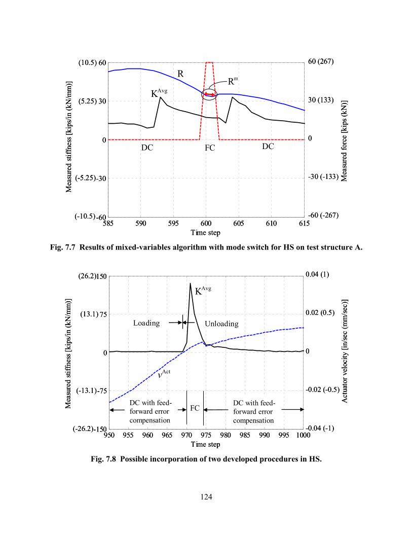
124
585 590 595 600 605 610 615-60
-30
0
30
60
Time step
(5.25)
(10.5)
(-10.5)
(-5.25)
Mea
sure
d sti
ffnes
s [ki
ps/in
(kN
/mm
)]60 (267)
30 (133)
0
-30 (-133)
-60 (-267)
Mea
sure
d fo
rce
[kip
s (kN
)]
AvgK
R
DC FC DC
mR
585 590 595 600 605 610 615-60
-30
0
30
60
Time step
(5.25)
(10.5)
(-10.5)
(-5.25)
Mea
sure
d sti
ffnes
s [ki
ps/in
(kN
/mm
)]60 (267)
30 (133)
0
-30 (-133)
-60 (-267)
Mea
sure
d fo
rce
[kip
s (kN
)]
AvgK
R
DC FC DC
mR
Fig. 7.7 Results of mixed-variables algorithm with mode switch for HS on test structure A.
950 955 960 965 970 975 980 985 990 995 1000-150
-75
0
75
150
Time step
(26.2)
(13.1)
(-13.1)
(-26.2)
0.04 (1)
0.02 (0.5)
0
-0.02 (-0.5)
-0.04 (-1)
Mea
sure
d sti
ffnes
s [ki
ps/in
(kN
/mm
)]
Act
uato
r vel
ocity
[in/
sec
(mm
/sec)
]
AvgK
Actv
DC FCDC with feed-forward error compensation
DC with feed-forward error compensation
Loading Unloading
Fig. 7.8 Possible incorporation of two developed procedures in HS.

125
7.4 SUMMARY
The two procedures presented in Chapter 6 are implemented on test structures A and B. Feed-
forward error compensation based on the correlation with the actuator velocity is implemented
on both test structures and a considerable improvement of the execution of the displacement
command signal is achieved as a result. Mixed-variables control is implemented in the hybrid
simulation system and is applied on test structure B with mode switch between force and
displacement control, and the test is conducted smoothly provided that some restrictions are
enforced in the mode-switch decision-making procedure and that the tuning of the actuator in
force control is adequate. The displacement control error compensation scheme is found to be
complementary in nature with the mixed-variables control and it is proposed to apply the two
procedures alternately to achieve a more accurate execution and a generalized framework of the
online experiments.

8 Structural Evaluation and Comparisons
This chapter addresses phases S-1, S-2, and S-3 for test structure A (see Fig. 1.2), as well as the
structural performance of test structure B. The results of test structure A are discussed in terms of
its global response, crack pattern, and mode of failure, the structural contribution of the URM
infill wall and the local behavior represented by beam-to-column joint rotations. In the case of
test structure B, the results are discussed in terms of the global behavior and mode of failure.
Comparisons to the corresponding ST experiments for the two test structures A and B are
conducted aiming to compare the two testing methods, namely HS and ST.
8.1 TEST STRUCTURE A: PHASE S-1
Test Structure A, described in Chapter 4, is subjected to a number of strong motions and
categorized into three phases (see Fig. 4.4) based on the state of the test structure, described in
Section 4.3. The first phase, namely S-1, represents the test structure with URM infill wall in the
middle frame and all columns are post-tensioned.
The execution time for each integration time step is selected as dt = 0.2 sec. This
execution time for the algorithm in DC is sufficient to perform the numerical integration, send
the displacement command signal, and receive the restoring-force feedback signal without any
delay. Since the time step of the numerical integration tΔ = 0.0025 sec is selected for all runs in
S-1, testing is performed at a rate of 800025.02.0 ==Δ= ttTR d times slower than real time.
Note that in the following discussion, the low-level seismic excitation TAR-1, which is
conducted for the purpose of checking the proper functionality of the data-acquisition system, is
not discussed.

128
8.1.1 Force-Displacement Behavior
The global response of the test structure is represented by the total base shear versus lateral
displacement at the expected level of the total inertial force due to ground shaking of the one-
story test structure. The total base shear is estimated as the sum of the lateral restoring forces in
the RC frames measured from the actuators force feedbacks and the numerically simulated
damping forces. The total base shear is considered in this section, since it is the quantity that can
be compared with its equivalent in the ST test results (Hashemi and Mosalam 2007), where the
damping force cannot be separated from the total base shear force without a number of uncertain
assumptions. The displacements are measured at the height of the load application on the frames.
The stiffness values in the following discussion are estimated based on the average tangent slope
at distinct stages of the applied strong motion. These stages are defined for each corresponding
stiffness value in the following paragraphs, and each of the average tangent slopes is evaluated
over all the recorded points of the loading branches of the force-displacement cycles, within that
stage, using the least-squares method to obtain a best linear fit of the stiffness value in question.
In TAR-2, TAR-3, and TAR-4, and for the initial range of low-level excitation in each
strong motion, where the total base shear forces are lower than ±15 kips (±66.7 kN), the response
is characterized by a high initial stiffness SK ; refer to Table 8.1 and Figure 8.1. This high initial
stiffness is attributed to the static friction between the URM infill wall at its interface and the
surrounding RC frame. Due to the slow test rate at which the strong motion is applied, this static
friction is not overcome at a certain velocity threshold as expected in the ST experiment case.
Instead, this static friction is controlled by the static resistance due to the grinding of the particles
on the interface between the URM infill wall and the surrounding RC frame members. This high
initial stiffness starts at SK = 826 kips/in. (144.7 kN/mm) in TAR-2 (Table 8.1 and Fig. 8.1(a)),
representing 85% of the value obtained from the pull-back test in Section 4.11, where the
stiffness for the whole test structure, i.e., F1I and two F2B frames with a connecting RC slab, is
evaluated at 977 kips/in. (171.1 kN/mm). This decrease is due to the difference in the amplitude
and repetition of the excitation forces in these two tests. While in the pull-back test, the sum of
the forces applied on the test structure is only 11 kips (22 kN), described in Section 4.11, the
total force applied in TAR-2 in the range of the high stiffness due to static friction is 15 kips
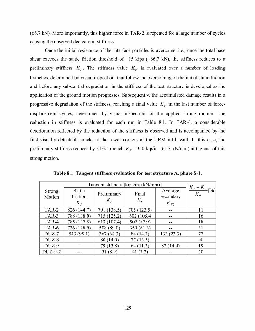
129
(66.7 kN). More importantly, this higher force in TAR-2 is repeated for a large number of cycles
causing the observed decrease in stiffness.
Once the initial resistance of the interface particles is overcome, i.e., once the total base
shear exceeds the static friction threshold of ±15 kips (±66.7 kN), the stiffness reduces to a
preliminary stiffness PK . The stiffness value PK is evaluated over a number of loading
branches, determined by visual inspection, that follow the overcoming of the initial static friction
and before any substantial degradation in the stiffness of the test structure is developed as the
application of the ground motion progresses. Subsequently, the accumulated damage results in a
progressive degradation of the stiffness, reaching a final value FK in the last number of force-
displacement cycles, determined by visual inspection, of the applied strong motion. The
reduction in stiffness is evaluated for each run in Table 8.1. In TAR-6, a considerable
deterioration reflected by the reduction of the stiffness is observed and is accompanied by the
first visually detectable cracks at the lower corners of the URM infill wall. In this case, the
preliminary stiffness reduces by 31% to reach FK =350 kip/in. (61.3 kN/mm) at the end of this
strong motion.
Table 8.1 Tangent stiffness evaluation for test structure A, phase S-1.
Tangent stiffness [kips/in. (kN/mm)] Strong Motion
Static friction
SK
PreliminaryPK
Final FK
Average secondary
2FK
[%]P
FP
KKK −
TAR-2 826 (144.7) 791 (138.5) 705 (123.5) -- 11 TAR-3 788 (138.0) 715 (125.2) 602 (105.4 -- 16 TAR-4 785 (137.5) 613 (107.4) 502 (87.9) -- 18 TAR-6 736 (128.9) 508 (89.0) 350 (61.3) -- 31 DUZ-7 543 (95.1) 367 (64.3) 84 (14.7) 133 (23.3) 77 DUZ-8 -- 80 (14.0) 77 (13.5) -- 4 DUZ-9 -- 79 (13.8) 64 (11.2) 82 (14.4) 19
DUZ-9-2 -- 51 (8.9) 41 (7.2) -- 20

130
-0.5 -0.25 0 0.25 0.5-150
-100
-50
0
50
100
150
Displacement [in]
Forc
e [k
ips]
-10 -5 0 5 10
-600
-400
-200
0
200
400
600
Displacement [mm]
Forc
e [k
N]
KS = 826 kips/in
KP = 791 kips/in
KF = 705 kips/in
-0.5 -0.25 0 0.25 0.5-150
-100
-50
0
50
100
150
Displacement [in]
Forc
e [k
ips]
-10 -5 0 5 10
-600
-400
-200
0
200
400
600
Displacement [mm]
Forc
e [k
N]
KS = 826 kips/in
KP = 791 kips/in
KF = 705 kips/in
-0.5 -0.25 0 0.25 0.5-150
-100
-50
0
50
100
150
Displacement [in]
Forc
e [k
ips]
-10 -5 0 5 10
-600
-400
-200
0
200
400
600
Displacement [mm]
Forc
e [k
N]
KS = 788 kips/in
KP = 715 kips/in
KF = 602 kips/in
-0.5 -0.25 0 0.25 0.5-150
-100
-50
0
50
100
150
Displacement [in]
Forc
e [k
ips]
-10 -5 0 5 10
-600
-400
-200
0
200
400
600
Displacement [mm]
Forc
e [k
N]
KS = 788 kips/in
KP = 715 kips/in
KF = 602 kips/in
(a) TAR-2 (b) TAR-3
-0.5 -0.25 0 0.25 0.5-150
-100
-50
0
50
100
150
Displacement [in]
Forc
e [k
ips]
-10 -5 0 5 10
-600
-400
-200
0
200
400
600
Displacement [mm]
Forc
e [k
N]
KS = 785 kips/in
KP = 613 kips/in
KF = 502 kips/in
-0.5 -0.25 0 0.25 0.5-150
-100
-50
0
50
100
150
Displacement [in]
Forc
e [k
ips]
-10 -5 0 5 10
-600
-400
-200
0
200
400
600
Displacement [mm]
Forc
e [k
N]
KS = 785 kips/in
KP = 613 kips/in
KF = 502 kips/in
-0.5 -0.25 0 0.25 0.5-150
-100
-50
0
50
100
150
Displacement [in]
Forc
e [k
ips]
-10 -5 0 5 10
-600
-400
-200
0
200
400
600
Displacement [mm]
Forc
e [k
N]
KS = 736 kips/in
KP = 508 kips/in
KF = 350 kips/in
-0.5 -0.25 0 0.25 0.5-150
-100
-50
0
50
100
150
Displacement [in]
Forc
e [k
ips]
-10 -5 0 5 10
-600
-400
-200
0
200
400
600
Displacement [mm]
Forc
e [k
N]
KS = 736 kips/in
KP = 508 kips/in
KF = 350 kips/in
(c) TAR-4 (d) TAR-6
Fig. 8.1 Total base shear versus lateral displacement for test structure A, phase S-1, TAR-2 to TAR-6 (1 kip/in.= 0.175 kN/mm).
In DUZ-7, the high initial stiffness due to static friction is much smaller with SK = 543
kips/in. (95.1 kN/mm) due to the increasingly defined cracking at the smoothened URM infill
wall interface with the surrounding RC frame members due to several grinding loading cycles,
(Table 8.1 and Fig. 8.2(a)). The preliminary stiffness is 367 kips/in. (64.3 kN/mm)
approximately corresponding to the final stiffness of the previous level, i.e., 350 kip/in. (61.3
kN/mm) for TAR-6. The first major crack in the URM infill wall occurs with a sudden drop in
stiffness. At this point, a stiffening behavior with pinched loops characterizes the response with a
low stiffness FK at the origin, where the URM infill wall is not effectively engaged, and higher
secondary stiffness 2FK . This secondary stiffness is evaluated over the higher stiffness parts of
the loading branches, determined by visual inspection. Note that the transition from FK to 2FK

131
coincides with the closing of the gaps between the URM infill wall and the surrounding RC
frame members. At the end of DUZ-7, a clear crack pattern in the URM infill wall is observed as
shown in Figure 8.3(a).
-4 -3 -2 -1 0 1 2 3 4
-200
-100
0
100
200
Displacement [in]
Forc
e [k
ips]
-100 -50 0 50 100
-1000
-500
0
500
1000
Displacement [mm]
Forc
e [k
N]
KS = 543 kips/in
KP = 367 kips/in
KF = 84 kips/in
KF2 = 146 kips/in
KF2 = 119 kips/in
+
-
-4 -3 -2 -1 0 1 2 3 4
-200
-100
0
100
200
Displacement [in]
Forc
e [k
ips]
-100 -50 0 50 100
-1000
-500
0
500
1000
Displacement [mm]
Forc
e [k
N]
KS = 543 kips/in
KP = 367 kips/in
KF = 84 kips/in
KF2 = 146 kips/in
KF2 = 119 kips/in
-4 -3 -2 -1 0 1 2 3 4
-200
-100
0
100
200
Displacement [in]
Forc
e [k
ips]
-100 -50 0 50 100
-1000
-500
0
500
1000
Displacement [mm]
Forc
e [k
N]
KS = 543 kips/in
KP = 367 kips/in
KF = 84 kips/in
KF2 = 146 kips/in
KF2 = 119 kips/in
+
-
-4 -3 -2 -1 0 1 2 3 4
-200
-100
0
100
200
Displacement [in]
Forc
e [k
ips]
-100 -50 0 50 100
-1000
-500
0
500
1000
Displacement [mm]
Forc
e [k
N]
KP = 80 kips/in
KF = 77 kips/in
-4 -3 -2 -1 0 1 2 3 4
-200
-100
0
100
200
Displacement [in]
Forc
e [k
ips]
-100 -50 0 50 100
-1000
-500
0
500
1000
Displacement [mm]
Forc
e [k
N]
KP = 80 kips/in
KF = 77 kips/in
(a) DUZ-7 (b) DUZ-8
-4 -3 -2 -1 0 1 2 3 4
-200
-100
0
100
200
Displacement [in]
Forc
e [k
ips]
-100 -50 0 50 100
-1000
-500
0
500
1000
Displacement [mm]
Forc
e [k
N]
KP = 79 kips/in
KF = 64 kips/in
KF2 = 81 kips/in
KF2 = 84 kips/in
+
-
-4 -3 -2 -1 0 1 2 3 4
-200
-100
0
100
200
Displacement [in]
Forc
e [k
ips]
-100 -50 0 50 100
-1000
-500
0
500
1000
Displacement [mm]
Forc
e [k
N]
KP = 79 kips/in
KF = 64 kips/in
KF2 = 81 kips/in
KF2 = 84 kips/in
-4 -3 -2 -1 0 1 2 3 4
-200
-100
0
100
200
Displacement [in]
Forc
e [k
ips]
-100 -50 0 50 100
-1000
-500
0
500
1000
Displacement [mm]
Forc
e [k
N]
KP = 79 kips/in
KF = 64 kips/in
KF2 = 81 kips/in
KF2 = 84 kips/in
+
-
-4 -3 -2 -1 0 1 2 3 4
-200
-100
0
100
200
Displacement [in]
Forc
e [k
ips]
-100 -50 0 50 100
-1000
-500
0
500
1000
Displacement [mm]
Forc
e [k
N]
KP = 51 kips/in
KF = 41 kips/in
-4 -3 -2 -1 0 1 2 3 4
-200
-100
0
100
200
Displacement [in]
Forc
e [k
ips]
-100 -50 0 50 100
-1000
-500
0
500
1000
Displacement [mm]
Forc
e [k
N]
KP = 51 kips/in
KF = 41 kips/in
(c) DUZ-9 (d) DUZ-9-2
Fig. 8.2 Total base shear versus lateral displacement for test structure A, phase S-1, DUZ-7 to DUZ-9-2 (1 kip/in.= 0.175 kN/mm).
(a) After DUZ-7 (b) After DUZ-9-2 (final state)
Fig. 8.3 Cracking patterns of URM infill wall in test structure A, phase S-1.

132
In DUZ-8 (Fig. 8.2(b)), the high initial stiffness due to static friction is absent and the
URM infill wall is nearly not engaged in the response. This is confirmed by the absence of the
pinching behavior observed in DUZ-7, and the maximum lateral drift is only slightly higher than
that in DUZ-7. Furthermore, the crack pattern does not differ significantly from the one at the
end of DUZ-7 and the stiffness is only slightly reduced by only 4% as shown in Table 8.1. In
DUZ-9, the strong motion excites the test structure beyond the maximum drift reached in DUZ-8
and the pinching behavior reappears, implying the reengagement of the damaged URM infill
wall but with less lateral load resistance. At the end of this level, a partial collapse of the URM
infill wall occurs. In DUZ-9-2, which is the repeat of DUZ-9, the behavior returns to the one
observed in DUZ-8 with little contribution from the disintegrated URM infill wall. The final
crack pattern is shown in Figure 8.3(b), where the shaded areas denote the collapsed parts of the
URM infill wall. Typical diagonal cracking and crushing at the corners is clearly observed and
three major horizontal cracks, along the URM infill wall height, complete the crack pattern and
form the failure mechanism, which allows the URM infill wall to deform in its own plane
without carrying any substantial part of the applied lateral load. Therefore, in DUZ-9-2, one
concludes that the RC frames are effectively the only lateral load-resisting elements.
8.1.2 URM Infill Wall Contribution
The URM infill wall contribution to the structural response of test structure A is assessed. The
shear force in the URM infill wall WF is estimated as the difference between the restoring forces,
measured from the load cells directly attached to the actuators, in the infilled RC frame and that
in the RC bare frame. The peak values of the restoring force in the URM infill wall and the sum
of the restoring forces in the three RC frames comprising the one-story test structure are plotted
in Figure 8.4. In this figure, a distinction is made between results recorded at the maximum total
base shear (Fig. 8.4(a)), and at the maximum lateral displacement (Fig. 8.4(b)). The
corresponding ratio in percentage of the restoring force resisted by the URM infill wall alone
with respect to that resisted by the entire URM infilled RC test structure is shown in Figure
8.4(c) and the values are reported in Table 8.2.

133
0
50
100
150
200R
esto
ring
forc
e [k
ips]
0
200
400
600
800URM wallRC frames
TAR
-2
TAR
-3
TAR
-4
TAR
-6
DU
Z-7
DU
Z-8
DU
Z-9
DU
Z-9-
2
Res
torin
g fo
rce
[kN
]
0
50
100
150
200R
esto
ring
forc
e [k
ips]
0
200
400
600
800URM wallRC frames
TAR
-2
TAR
-3
TAR
-4
TAR
-6
DU
Z-7
DU
Z-8
DU
Z-9
DU
Z-9-
2
Res
torin
g fo
rce
[kN
]
TAR
-2
TAR
-3
TAR
-4
TAR
-6
DU
Z-7
DU
Z-8
DU
Z-9
DU
Z-9-
2
0
50
100
150
200
0
200
400
600
800
Res
torin
g fo
rce
[kN
]
URM wallRC frames
Res
torin
g fo
rce
[kip
s]
TAR
-2
TAR
-3
TAR
-4
TAR
-6
DU
Z-7
DU
Z-8
DU
Z-9
DU
Z-9-
2
0
50
100
150
200
0
200
400
600
800
Res
torin
g fo
rce
[kN
]
URM wallRC frames
Res
torin
g fo
rce
[kip
s]
(a) At peak base shear (b) At peak lateral displacement
0
25
50
75
100
URM
wal
l con
tribu
tion
[%]
Peak base shearPeak Displacement
TAR
-2
TAR
-3
TAR
-4
TAR
-6
DU
Z-7
DU
Z-8
DU
Z-9
DU
Z-9-
2
0
25
50
75
100
URM
wal
l con
tribu
tion
[%]
Peak base shearPeak Displacement
TAR
-2
TAR
-3
TAR
-4
TAR
-6
DU
Z-7
DU
Z-8
DU
Z-9
DU
Z-9-
2
(c) Ratio of base shear contribution of URM infill wall
Fig. 8.4 Contribution of URM infill wall and RC frames to restoring forces.
The contribution of the URM infill wall before cracking (up to TAR-6) represents the
major share of the structural components in resisting the total base shear. This contribution starts
at about 85% at TAR-2 and gradually decreases to reach 74% at TAR-6. In DUZ-7, where major
cracking in the URM infill wall occurs, the decrease of the URM infill wall contribution is
substantial and continues, in subsequent test levels, until the RC bare frames control the
response, whereas the URM infill wall contribution reaches only 9% in DUZ-9-2. Note that the
difference between the two ratios, at peak displacement and at peak base shear, is more apparent
in the two events, DUZ-7 and to a lesser extent DUZ-9, where the behavior of the structural
system undergoes considerable deterioration of an almost intact URM infill wall and a
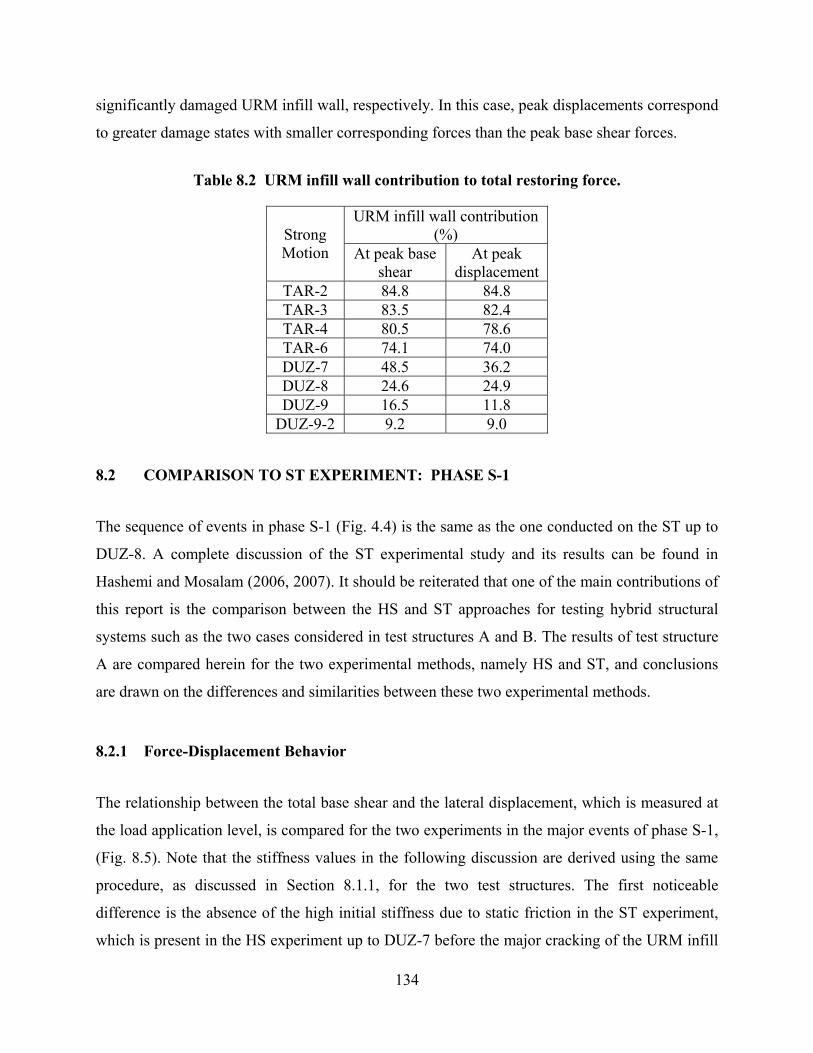
134
significantly damaged URM infill wall, respectively. In this case, peak displacements correspond
to greater damage states with smaller corresponding forces than the peak base shear forces.
Table 8.2 URM infill wall contribution to total restoring force.
URM infill wall contribution (%) Strong
Motion At peak base shear
At peak displacement
TAR-2 84.8 84.8 TAR-3 83.5 82.4 TAR-4 80.5 78.6 TAR-6 74.1 74.0 DUZ-7 48.5 36.2 DUZ-8 24.6 24.9 DUZ-9 16.5 11.8
DUZ-9-2 9.2 9.0
8.2 COMPARISON TO ST EXPERIMENT: PHASE S-1
The sequence of events in phase S-1 (Fig. 4.4) is the same as the one conducted on the ST up to
DUZ-8. A complete discussion of the ST experimental study and its results can be found in
Hashemi and Mosalam (2006, 2007). It should be reiterated that one of the main contributions of
this report is the comparison between the HS and ST approaches for testing hybrid structural
systems such as the two cases considered in test structures A and B. The results of test structure
A are compared herein for the two experimental methods, namely HS and ST, and conclusions
are drawn on the differences and similarities between these two experimental methods.
8.2.1 Force-Displacement Behavior
The relationship between the total base shear and the lateral displacement, which is measured at
the load application level, is compared for the two experiments in the major events of phase S-1,
(Fig. 8.5). Note that the stiffness values in the following discussion are derived using the same
procedure, as discussed in Section 8.1.1, for the two test structures. The first noticeable
difference is the absence of the high initial stiffness due to static friction in the ST experiment,
which is present in the HS experiment up to DUZ-7 before the major cracking of the URM infill

135
wall, discussed in Section 8.1.1. This is attributed to the high velocity at which the real-time ST
experiment is conducted which allows overcoming the static friction much more efficiently than
in the HS with slower rate of load application. The second difference is the distinctly higher
stiffness values of the HS test structure, e.g., in TAR-6, PK = 508 kips/in. (89.0 kN/mm) in HS,
and PK = 364 kips/in. (63.7 kN/mm) in the ST, i.e., 1.4 times larger (Table 8.3).
It should be stressed that all feasible efforts were made for the test structure A used in the
HS and that used in the ST to be as close, in structural and material properties, as practically
possible. Note that the concrete compressive strength is similar, the reinforcing steel is obtained
from the same mill, and the masonry units are acquired from the same patch. However, the URM
infill wall, which was built by the same professional masons for the HS and ST experiments, is
the potential candidate as being the source of difference between the test structures used in these
two experiments, particularly from the construction point of view. It is known that the level of
tightly filling the space defined by the RC frame with URM infill wall depends on the masons
skills and boundary conditions, e.g., having a roof represented by the connecting RC slab with its
lateral and vertical stiffness contributions as in the ST experiment versus not having this physical
slab as in the HS experiment where the slab is numerically simulated only in the lateral direction.
Therefore, the RC slab and the URM infill wall are potential sources of discrepancy between the
two test structures used for the HS and ST experiments. This is discussed in more detail in
Section 8.2.2.

136
-0.5 -0.25 0 0.25 0.5-150
-100
-50
0
50
100
150
Displacement [in]
Forc
e [k
ips]
-10 -5 0 5 10
-600
-400
-200
0
200
400
600
Displacement [mm]
Forc
e [k
N]
KS = 736 kips/in
KP = 508 kips/in
KF = 350 kips/in
-0.5 -0.25 0 0.25 0.5-150
-100
-50
0
50
100
150
Displacement [in]
Forc
e [k
ips]
-10 -5 0 5 10
-600
-400
-200
0
200
400
600
Displacement [mm]
Forc
e [k
N]
KS = 736 kips/in
KP = 508 kips/in
KF = 350 kips/in
-0.5 -0.25 0 0.25 0.5-150
-100
-50
0
50
100
150
Displacement [in]
Forc
e [k
ips]
-10 -5 0 5 10
-600
-400
-200
0
200
400
600
Displacement [mm]
Forc
e [k
N]
KF = 289 kips/in
KP = 364 kips/in
-0.5 -0.25 0 0.25 0.5-150
-100
-50
0
50
100
150
Displacement [in]
Forc
e [k
ips]
-10 -5 0 5 10
-600
-400
-200
0
200
400
600
Displacement [mm]
Forc
e [k
N]
KF = 289 kips/in
KP = 364 kips/in
(a) TAR-6 (HS) (b) TAR-6 (ST)
-3 -2 -1 0 1 2 3
-200
-100
0
100
200
Displacement [in]
Forc
e [k
ips]
-50 0 50
-1000
-500
0
500
1000
Displacement [mm]Fo
rce
[kN
]
KS = 543 kips/in
KP = 367 kips/in
KF = 84 kips/in
KF2 = 146 kips/in
KF2 = 119 kips/in
+
-
-3 -2 -1 0 1 2 3
-200
-100
0
100
200
Displacement [in]
Forc
e [k
ips]
-50 0 50
-1000
-500
0
500
1000
Displacement [mm]Fo
rce
[kN
]
KS = 543 kips/in
KP = 367 kips/in
KF = 84 kips/in
KF2 = 146 kips/in
KF2 = 119 kips/in
+
-
-2 -1 0 1 2
-200
-100
0
100
200
Displacement [in]
Forc
e [k
ips]
-50 0 50
-1000
-500
0
500
1000
Displacement [mm]
Forc
e [k
N]
KP = 278 kips/in
KF = 59 kips/in
KF2 = 160 kips/in
KF2 = 159 kips/in
+
-
-2 -1 0 1 2
-200
-100
0
100
200
Displacement [in]
Forc
e [k
ips]
-50 0 50
-1000
-500
0
500
1000
Displacement [mm]
Forc
e [k
N]
KP = 278 kips/in
KF = 59 kips/in
KF2 = 160 kips/in
KF2 = 159 kips/in
+
-
(c) DUZ-7 (HS) (d) DUZ-7 (ST)
-3 -2 -1 0 1 2 3
-200
-100
0
100
200
Displacement [in]
Forc
e [k
ips]
-50 0 50
-1000
-500
0
500
1000
Displacement [mm]
Forc
e [k
N]
KP = 80 kips/in
KF = 77 kips/in
-3 -2 -1 0 1 2 3
-200
-100
0
100
200
Displacement [in]
Forc
e [k
ips]
-50 0 50
-1000
-500
0
500
1000
Displacement [mm]
Forc
e [k
N]
KP = 80 kips/in
KF = 77 kips/in
-3 -2 -1 0 1 2 3
-200
-100
0
100
200
Displacement [in]
Forc
e [k
ips]
-50 0 50
-1000
-500
0
500
1000
Displacement [mm]
Forc
e [k
N]
KP = 116 kips/in
KF = 63 kips/in
-3 -2 -1 0 1 2 3
-200
-100
0
100
200
Displacement [in]
Forc
e [k
ips]
-50 0 50
-1000
-500
0
500
1000
Displacement [mm]
Forc
e [k
N]
KP = 116 kips/in
KF = 63 kips/in
e) DUZ-8 (HS) f) DUZ-8 (ST)
Fig. 8.5 Total base shear versus lateral displacement comparisons for test structure A, phase S-1 (1 kip/in.=0.175 kN/mm).
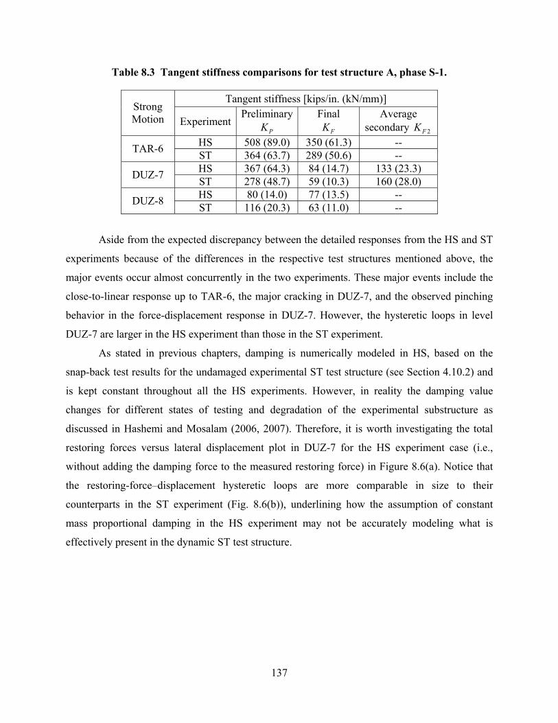
137
Table 8.3 Tangent stiffness comparisons for test structure A, phase S-1.
Tangent stiffness [kips/in. (kN/mm)] Strong Motion Experiment
PreliminaryPK
Final FK
Average secondary 2FK
HS 508 (89.0) 350 (61.3) -- TAR-6 ST 364 (63.7) 289 (50.6) -- HS 367 (64.3) 84 (14.7) 133 (23.3) DUZ-7 ST 278 (48.7) 59 (10.3) 160 (28.0) HS 80 (14.0) 77 (13.5) -- DUZ-8 ST 116 (20.3) 63 (11.0) --
Aside from the expected discrepancy between the detailed responses from the HS and ST
experiments because of the differences in the respective test structures mentioned above, the
major events occur almost concurrently in the two experiments. These major events include the
close-to-linear response up to TAR-6, the major cracking in DUZ-7, and the observed pinching
behavior in the force-displacement response in DUZ-7. However, the hysteretic loops in level
DUZ-7 are larger in the HS experiment than those in the ST experiment.
As stated in previous chapters, damping is numerically modeled in HS, based on the
snap-back test results for the undamaged experimental ST test structure (see Section 4.10.2) and
is kept constant throughout all the HS experiments. However, in reality the damping value
changes for different states of testing and degradation of the experimental substructure as
discussed in Hashemi and Mosalam (2006, 2007). Therefore, it is worth investigating the total
restoring forces versus lateral displacement plot in DUZ-7 for the HS experiment case (i.e.,
without adding the damping force to the measured restoring force) in Figure 8.6(a). Notice that
the restoring-force–displacement hysteretic loops are more comparable in size to their
counterparts in the ST experiment (Fig. 8.6(b)), underlining how the assumption of constant
mass proportional damping in the HS experiment may not be accurately modeling what is
effectively present in the dynamic ST test structure.

138
-2 -1 0 1 2
-200
-100
0
100
200
Displacement [in]
Forc
e [k
ips]
-50 0 50
-1000
-500
0
500
1000
Displacement [mm]
Forc
e [k
N]
-2 -1 0 1 2
-200
-100
0
100
200
Displacement [in]
Forc
e [k
ips]
-50 0 50
-1000
-500
0
500
1000
Displacement [mm]
Forc
e [k
N]
(a) Restoring force versus lateral displacement (HS)
(b) Total base shear versus lateral displacement (ST)
Fig. 8.6 DUZ-7 comparisons for test structure A, phase S-1.
In DUZ-8 (Figs. 8.5(e)–(f) and Table 8.3), the results from HS and ST diverge
significantly. In HS, where the URM infill wall is close to being structurally insignificant in
DUZ-7 (average 2FK = 133 kips/in. (23.3 kN/mm) for the positive and negative excursions
compared to average 2FK = 160 kips/in. (28.0 kN/mm) in the ST), no additional damage or
significant degradation occurs in DUZ-8. On the other hand, in ST, a 58% reduction in the
preliminary stiffness PK is observed from DUZ-7 to DUZ-8 and the cracking pattern of the
URM infill wall develops further accompanied by partial collapse of significant parts of the
URM infill wall. This is attributed to the slow velocity and the associated low acceleration at
which the HS test is conducted compared to the ST, where the in-plane and probably more
importantly the out-of-plane inertial forces of the mass of the disintegrated masonry parts do not
sufficiently develop to dislocate these parts from the rest of the URM infill wall. Moreover, the
interlocking action and the associated friction between these parts is large enough to hold the
URM infill wall together under slow loading rates in the HS experiment, which is not the case in
the ST experiment.
The cracking patterns of the two URM infill walls for HS and ST at the end of DUZ-7
(Figs. 8.7(a)–(b)) hold the same general features comprising diagonal cracks, crushing at the
corners, and horizontal cracking. It is to be noted that one horizontal crack is formed in the ST at
approximately one third the height of the URM infill wall, and two horizontal cracks are formed
in the HS at approximately one and two thirds the height of the URM infill wall. These
horizontal cracks (along the mortar bed joints) link the diagonal ones and form the failure

139
mechanism of the URM infill wall, matching the shape of the proposed compression-only strut
model in Mosalam (1996a). The length of these horizontal (bed joint) cracks depends on the
aspect ratio of the URM infill wall panel. However, while dynamically, the URM infill wall
disintegrates significantly in DUZ-8 and partial collapse is observed, pseudo-dynamically, two
higher level runs (DUZ-9 and DUZ-9-2) are needed to visually reach a comparable partial
collapse to that after DUZ-8 in the ST experiment (Figs. 8.7(c)–(d)) due to factors related to the
different loading rates at which the two experiments are conducted as discussed above.
(a) After DUZ-7 (HS) (b) After DUZ-7 (ST)
(c) After DUZ-9-2 (HS) (d) After DUZ-8 (ST)
Fig. 8.7 Cracking patterns developed in URM infill wall in HS and ST experiments (shaded areas indicate dislocated parts of wall).
Comparing the cracking patterns from the HS to those from the ST in a more detailed
level reveals an important difference. In the HS, several vertical cracks took place in the upper
edge of the URM infill wall due to the interaction with the RC beam of the bounding frame.
These cracks are attributed to the limited flexural stiffness of the RC beam which tends to deflect
vertically under the lateral load of the frame, causing contact in the compression corner and loss
of contact in the far corner (Fig. 8.8). This deformed shape produces a cantilever action in the
URM infill wall and vertical cracks are triggered. This phenomenon was first observed by

140
Mosalam (1996a) when testing steel frames with URM infill walls. In the ST experiments, this is
not observed because of the much higher stiffness of the RC beam due to the effect of the
connecting slab.
Fig. 8.8 Deformation of URM infill wall and bounding RC frame.
The peak global response, represented by the maximum total base shear at different levels
of strong motion and its corresponding lateral displacement (Fig. 8.9(a)), as well as the
maximum lateral displacement and its corresponding total base shear (Fig. 8.9(b)) are compared
for the HS and ST experiments. Note that the plotted peak values for the two experiments do not
necessarily occur at the same time during the application of the strong motion.
Up to TAR-6, where the response in the two experiments is close-to-linear with very few
visible signs of damage or degradation, the peak lateral displacements in the ST experiment are
distinctly larger than in HS (1.6 to 1.8 times larger), while the corresponding base shears are
around the same magnitudes. This is in accordance with the higher tangent stiffness in HS,
illustrated in Figure 8.5 and Table 8.3. In DUZ-7, the HS test structure is subjected to larger peak
lateral displacement and peak base shear than those of the ST test and both URM infill walls in
the two tests undergo major cracking. In DUZ-8, as discussed previously, the complete
disintegration of the URM infill wall dynamically is accompanied by a larger lateral
displacement demand, while pseudo-dynamically, the pseudo-velocity and pseudo-acceleration
are not enough to dislocate the disintegrated parts of the URM infill wall. Therefore, much larger
peak lateral displacement is recorded during DUZ-8 for the ST test than that for the HS test (Fig.
8.9).

141
TAR
-2
TAR
-3
TAR
-4
TAR
-6
DU
Z-7
DU
Z-80
0.5
1
1.5
2
2.5
3D
ispla
cem
ent [
in]
0
20
40
60
Disp
lace
men
t [m
m]
HSST
TAR
-2
TAR
-3
TAR
-4
TAR
-6
DU
Z-7
DU
Z-80
0.5
1
1.5
2
2.5
3D
ispla
cem
ent [
in]
0
20
40
60
Disp
lace
men
t [m
m]
HSST
TAR
-2
TAR
-3
TAR
-4
TAR
-6
DU
Z-7
DU
Z-8
TAR
-2
TAR
-3
TAR
-4
TAR
-6
DU
Z-7
DU
Z-80
0.5
1
1.5
2
2.5
3D
ispla
cem
ent [
in]
0
20
40
60
Disp
lace
men
t [m
m]
HSST
TAR
-2
TAR
-3
TAR
-4
TAR
-6
DU
Z-7
DU
Z-80
0.5
1
1.5
2
2.5
3D
ispla
cem
ent [
in]
0
20
40
60
Disp
lace
men
t [m
m]
HSST
TAR
-2
TAR
-3
TAR
-4
TAR
-6
DU
Z-7
DU
Z-8
TAR
-2
TAR
-3
TAR
-4
TAR
-6
DU
Z-7
DU
Z-80
50
100
150
200
Tota
l bas
e sh
ear [
kips
]
0
200
400
600
800
Tota
l bas
e sh
ear [
kN]
HSST
TAR
-2
TAR
-3
TAR
-4
TAR
-6
DU
Z-7
DU
Z-80
50
100
150
200
Tota
l bas
e sh
ear [
kips
]
0
200
400
600
800
Tota
l bas
e sh
ear [
kN]
HSST
TAR
-2
TAR
-3
TAR
-4
TAR
-6
DU
Z-7
DU
Z-8
(a) At peak base shear
TAR
-2
TAR
-3
TAR
-4
TAR
-6
DU
Z-7
DU
Z-80
0.5
1
1.5
2
2.5
3
Disp
lace
men
t [in
]
0
20
40
60D
ispla
cem
ent [
mm
]
HSST
TAR
-2
TAR
-3
TAR
-4
TAR
-6
DU
Z-7
DU
Z-80
0.5
1
1.5
2
2.5
3
Disp
lace
men
t [in
]
0
20
40
60D
ispla
cem
ent [
mm
]
HSST
TAR
-2
TAR
-3
TAR
-4
TAR
-6
DU
Z-7
DU
Z-8
TAR
-2
TAR
-3
TAR
-4
TAR
-6
DU
Z-7
DU
Z-80
0.5
1
1.5
2
2.5
3
Disp
lace
men
t [in
]
0
20
40
60D
ispla
cem
ent [
mm
]
HSST
TAR
-2
TAR
-3
TAR
-4
TAR
-6
DU
Z-7
DU
Z-80
0.5
1
1.5
2
2.5
3
Disp
lace
men
t [in
]
0
20
40
60D
ispla
cem
ent [
mm
]
HSST
TAR
-2
TAR
-3
TAR
-4
TAR
-6
DU
Z-7
DU
Z-8
TAR
-2
TAR
-3
TAR
-4
TAR
-6
DU
Z-7
DU
Z-8
TAR
-2
TAR
-3
TAR
-4
TAR
-6
DU
Z-7
DU
Z-80
50
100
150
200
Tota
l bas
e sh
ear [
kips
]
0
200
400
600
800
Tota
l bas
e sh
ear [
kN]
HSST
TAR
-2
TAR
-3
TAR
-4
TAR
-6
DU
Z-7
DU
Z-80
50
100
150
200
Tota
l bas
e sh
ear [
kips
]
0
200
400
600
800
Tota
l bas
e sh
ear [
kN]
HSST
TAR
-2
TAR
-3
TAR
-4
TAR
-6
DU
Z-7
DU
Z-8
(b) At peak lateral displacement
Fig. 8.9 Peak global responses in HS and ST experiments.
The lateral displacement time-history responses for TAR-6 in the two experiments using
HS and ST are presented in Figure 8.10. While the trend of the strong motion is similar
experiencing the same peaks, the pseudo-dynamic (HS) test structure lateral displacement is
clearly smaller than that for the dynamic (ST) test. However, the total base shear matches more
closely (Fig. 8.11), confirming the effect of the higher stiffness of the HS test structure than that
for the ST test structure as discussed previously.

142
0 5 10 15-0.5
-0.25
0
0.25
0.5
Disp
lace
men
t [in
]
-10
-5
0
5
10
Disp
lace
men
t [m
m]HS
0 5 10 15-0.5
-0.25
0
0.25
0.5
Time [sec]
Disp
lace
men
t [in
]
-10
-5
0
5
10
Disp
lace
men
t [m
m]ST
Fig. 8.10 Displacement time histories for TAR-6.
0 5 10 15-150
-100
-50
0
50
100
150
Bas
e sh
ear [
kips
]
-500
-250
0
250
500
Bas
e sh
ear [
kN]HS
0 5 10 15-150
-100
-50
0
50
100
150
Time [sec]
Bas
e sh
ear [
kips
]
-500
-250
0
250
500B
ase
shea
r [kN
]ST
Fig. 8.11 Total base shear time histories for TAR-6.

143
8.2.2 URM Infill Wall Contribution
The URM infill wall contribution is estimated in the two experiments and presented in Figures
8.12(a)–(b) at peak base shear and at peak lateral displacement, respectively. While in HS, the
restoring force in the wall wF is computed as the difference between the restoring forces in the
infilled and the bare frames which are readily available through the actuator force feedback
measured by the load cells, the estimation of these forces for the ST test structure involves a
number of procedures with underlying assumptions using measurements from accelerometers
and reinforcing bars strain gages (Hashemi and Mosalam 2006, 2007). The same trend is
observed in both experiments where the contribution of the URM infill wall is highest at the start
of the experiment and decreases gradually as the URM infill wall deteriorates. The larger
decrease is observed between TAR-6 and DUZ-7 as well as between DUZ-7 and DUZ-8 where
the URM infill wall undergoes major damage and its structural contribution to the test structure
decreases significantly. This is more apparent in Figure 8.12(b) where the peak lateral
displacements correspond to later stages within the same run.
TAR
-2
TAR
-3
TAR
-4
TAR
-6
DU
Z-7
DU
Z-80
25
50
75
100
URM
wal
l con
tribu
tion
[%]
HSST
TAR
-2
TAR
-3
TAR
-4
TAR
-6
DU
Z-7
DU
Z-80
25
50
75
100
URM
wal
l con
tribu
tion
[%]
HSST
UR
M in
fill w
all c
ontri
butio
n [%
]
TAR
-2
TAR
-3
TAR
-4
TAR
-6
DU
Z-7
DU
Z-8
TAR
-2
TAR
-3
TAR
-4
TAR
-6
DU
Z-7
DU
Z-80
25
50
75
100
URM
wal
l con
tribu
tion
[%]
HSST
TAR
-2
TAR
-3
TAR
-4
TAR
-6
DU
Z-7
DU
Z-80
25
50
75
100
URM
wal
l con
tribu
tion
[%]
HSST
UR
M in
fill w
all c
ontri
butio
n [%
]
TAR
-2
TAR
-3
TAR
-4
TAR
-6
DU
Z-7
DU
Z-8
TAR
-2
TAR
-3
TAR
-4
TAR
-6
DU
Z-7
DU
Z-80
25
50
75
100
URM
wal
l con
tribu
tion
[%]
HSST
TAR
-2
TAR
-3
TAR
-4
TAR
-6
DU
Z-7
DU
Z-80
25
50
75
100
URM
wal
l con
tribu
tion
[%]
HSST
UR
M in
fill w
all c
ontri
butio
n [%
]
TAR
-2
TAR
-3
TAR
-4
TAR
-6
DU
Z-7
DU
Z-8
TAR
-2
TAR
-3
TAR
-4
TAR
-6
DU
Z-7
DU
Z-80
25
50
75
100
URM
wal
l con
tribu
tion
[%]
HSST
TAR
-2
TAR
-3
TAR
-4
TAR
-6
DU
Z-7
DU
Z-80
25
50
75
100
URM
wal
l con
tribu
tion
[%]
HSST
UR
M in
fill w
all c
ontri
butio
n [%
]
TAR
-2
TAR
-3
TAR
-4
TAR
-6
DU
Z-7
DU
Z-8
(a) At peak total base shear (b) At peak lateral displacement
Fig. 8.12 URM infill wall contributions to restoring forces in HS and ST experiments.
The shear force wF versus the shear strain γ of the URM infill wall panel is shown in
Figure 8.13. In this figure, γ is calculated as shown in Figure 8.14, where 1Δ and 2Δ are
determined using the diagonal displacement measurements in the plane of the URM infill wall.
In TAR-6 (Figs. 8.13(a)–(b)), the two URM infill walls in the HS and ST experiments behave

144
very similarly (almost linearly) in terms of both magnitudes of shear strain and restoring force in
the URM infill wall. Considering the much larger lateral displacement observed in the ST
experiment (Fig. 8.10), which is also the case in the previous strong motion TAR-4, it is deduced
that the URM infill walls are of similar stiffness and their behaviors match closely. Therefore,
the difference in lateral displacement between the two test structures used in HS and ST
experiments is mainly due to larger lateral displacement (in the range of 0.0 to 0.2 in. (5.1 mm))
in the ST experiment corresponding to the total base shear required to engage the URM infill
wall to significantly contribute as a load-carrying element to the total restoring force. It is
interesting to note that the positive and negative peaks near the time of 5 sec in Figure 8.10 are
larger in the ST than the HS by about 0.2 in. (5.1 mm).
The larger lateral displacement in the ST experiment than in the HS may be attributed to
a number of factors: (1) the inherent variability taking place during construction because of
workmanship leading to a different level of tightness (filling) between the URM infill wall and
the surrounding frame with higher filling in the HS test structure; (2) the level of damage at the
corners of the URM infill wall where the impact between the wall and the surrounding frame
occurs in the ST test structure at a higher velocity causing more damage and therefore creating a
larger gap at the frame/wall interfaces; and (3) the different nature of the sliding mechanism and
the associated static versus dynamic friction, for the respective HS versus ST tests, at the
interface between the URM infill wall and the surrounding frame in the two experiments,
whether at the corners or at the top and bottom edges. While in the HS experiment, the slow test
rate causes the relative motion along the interface between the URM infill wall and the RC frame
members to be controlled by the grinding of the particles of the two surfaces against each other
to overcome the static friction, the sliding in the ST experiment is mainly controlled by the
velocity at which the static friction is overcome resulting in a more staggered sliding pattern,
(Fig. 8.15(b)). The outcome of the above three factors is that the surrounding RC frames in the
ST test structure deform more than those in the HS test structure. Therefore, it is concluded that
the reason for the higher stiffness in the HS than in ST experiment, discussed in Section 8.2.1
(see Fig. 8.5), is due to the above-mentioned factors rather than to a mere difference in material
properties.
Another potential source of discrepancies in the response of the two test structures for the
HS and ST experiments is related to the way viscous damping is modeled in the HS experiment.
As stated earlier, the numerical model for viscous damping in the HS case is assumed constant

145
(6.2% of the critical damping in the first mode of vibration) over the entire duration of the
experiment and is evaluated based on snap-back test results conducted on the undamaged ST test
structure. The estimation of viscous damping in the case of the ST test structure (Hashemi and
Mosalam 2006, 2007) shows a changing damping ratio (3% to 13%) as the test progresses and
the state of the test structure deteriorates.
-1 -0.5 0 0.5 1
x 10-3
-120
-60
0
60
120
γ
F w [k
ips]
-400
-200
0
200
400
F w [k
N]
-1 -0.5 0 0.5 1
x 10-3
-120
-60
0
60
120
γF w
[kip
s]
-400
-200
0
200
400
F w [k
N]
(a) TAR-6 (HS) (b) TAR-6 (ST)
-0.02 -0.01 0 0.01 0.02-120
-60
0
60
120
γ
F w [k
ips]
-400
-200
0
200
400
F w [k
N]
-0.02 -0.01 0 0.01 0.02-120
-60
0
60
120
γ
F w [k
ips]
-400
-200
0
200
400
F w [k
N]
(c) DUZ-7 (HS) (d) DUZ-7 (ST)
Fig. 8.13 Shear force versus shear strain of URM infill wall.
2Δ1ΔH
L
HLHL 22
12
2+Δ−Δ
=γ
Fig. 8.14 Estimation of shear strain from diagonal measurements ( 1Δ and 2Δ ).

146
In DUZ-7 (Figs. 8.13(c)–(d)), although the shear forces in the URM infill wall are quite
similar, the shear strain of the HS test structure is almost double the one recorded in the ST test
structure. This is attributed to the different cracking pattern in both experiments observed after
DUZ-7 (Figs. 8.7(a)–(b)). While diagonal cracking is quite similar, one major horizontal crack is
observed in the dynamic test, while an additional horizontal crack is observed in the pseudo-
dynamic test. This leads to additional planes of lateral motion for the URM infill wall in the HS
test than that in the ST test and accordingly results in a more flexible URM infill wall
mechanism leading to larger shear strains. The larger shear strains developed in HS than in ST
explain the two exceptions in Table 8.3 where 2FK in DUZ-7 and PK in DUZ-8 are larger for
the ST test structure, opposite to what is observed in all the other cases as discussed previously.
0 5 10 15 20-0.1
-0.05
0
0.05
0.1
Time [sec]
Slid
ing
[in]
-2
-1
0
1
2
Slid
ing
[mm
]
(a) HS
0 5 10 15 20-0.1
-0.05
0
0.05
0.1
Time [sec]
Slid
ing
[in]
-2
-1
0
1
2
Slid
ing
[mm
]
(b) ST
Fig. 8.15 URM infill wall sliding on bottom interface with respect to surrounding RC frame, TAR-6.
In addition to the increase in the observed shear strain, the additional horizontal (bed
joint) crack causes the URM infill wall to swell (dilate) vertically more than in the case of the ST
test structure. This increased dilation causes the URM infill wall to push against the top and
bottom RC frame members. The consequence of that phenomenon is two fold: (1) the friction at
the bottom and lower interfaces of the URM infill wall and the bounding frame is enhanced

147
further, supporting the earlier comments in that regard, and (2) the contact between the URM
infill wall and the top beam becomes stronger in the middle, where the horizontal cracks occur,
than at the corners, supporting the previously discussed cantilevering action which causes the
vertical splitting cracks in the URM infill wall near its upper edge.
8.3 TEST STRUCTURE A: PHASES S-2 AND S-3
Phases S-2 and S-3 (see Fig. 1.2) are applied to test structure A after the collapse of the URM
infill wall and its complete removal. At the end of phase S-1, the RC test structure, frame F2B
(refer to Section 4.3) shows minor signs of visible damage at the west and east beam-to-column
joints (Fig. 8.16), where the north direction is identified in Figure 4.16(a). As stated earlier, the
test structure is excited by a set of strong motions in phase S-2 (see Fig. 4.4), where the columns
post-tensioning axial force is maintained. On the other hand, at the start of phase S-3, the post-
tensioning force is removed and a new set of strong motions is applied, (see Fig. 4.4).
(a) West beam-to-column joint (b) East beam-to-column joint
Fig. 8.16 Observed damage in RC frame at beginning of phase S-2.
Figure 8.17(a) shows a plot of the peak lateral displacement and its corresponding total
base shear, while Figure 8.17(b) is a plot of the peak total base shear and its corresponding
lateral displacement, throughout phases S-2 and S-3. The maximum lateral displacement
recorded in phase S-2 during LPB-9-2[2] is 3.35 in. (85.1 mm) corresponding to 3.0% story drift
and the maximum recorded base shear is 151.6 kips (674.4 kN) during LPB-9[2]. After the
removal of the post-tensioning force in the columns, and at the end of phase S-3, the maximum

148
lateral displacement increases significantly, reaching 4.94 in. (125.5 mm) during LPB-9-7[3]
corresponding to 4.5% story drift and 7.17 in. (182.1 mm) during LPB-10[3] corresponding to
6.5% story drift, and the maximum base shear is reduced to 90.9 kips (404.3 kN) during LPB-9-
7[3] implying a significant degradation in strength and stiffness of the RC frame.
0 2 4 6 80
50
100
150
200
Displacement [in]
Forc
e [k
ips]
S-2S-3
0 50 100 150 200
0
200
400
600
800
Displacement [mm]
Forc
e [k
N]
LPB-9-2[2]
LPB-9[3]
LPB-10[3]
LPB-9-7[3]
0 2 4 6 80
50
100
150
200
Displacement [in]
Forc
e [k
ips]
0 50 100 150 200
0
200
400
600
800
Displacement [mm]
Forc
e [k
N]
LPB-9-2[2]
LPB-9[3] LPB-10[3]
LPB-9-7[3]
S-2S-3
0 2 4 6 80
50
100
150
200
Displacement [in]
Forc
e [k
ips]
0 50 100 150 200
0
200
400
600
800
Displacement [mm]
Forc
e [k
N]
LPB-9-2[2]
LPB-9[3] LPB-10[3]
LPB-9-7[3]
S-2S-3
(a) At peak lateral displacement (b) At peak total base shear
Fig. 8.17 Peak lateral displacement and peak total base shear for phases S-2 and S-3.
Figure 8.18 shows the total base shear versus lateral displacement relationship for level
LPB-9-2[2]. The bilinear behavior characterizing the response is attributed to the damage
developed in the foundations of the RC test structure, thus developing plastic hinges at these
column-to-footing joints. The low tangent stiffness 1K = 28 kips/in. (4.9 kN/mm) is observed to
dominate up to ±1 in. (±25.4 mm), i.e., in the range of lateral displacement where the plastic
hinges are developing in the foundations. This range is determined by the extent of the
reinforcing bars, yield penetration on the tension side, and the cracks closing on the compression
side. A higher stiffness 2K = 48 kips/in. (8.4 kN/mm) is estimated beyond that range, with an
increase of 71% of 2K relative to 1K . Note that these stiffness values are estimated using the
same procedure described in Section 8.1.1. Although the beam-to-column joints do not show any
major signs of visible damage up to the completion of phase S-2 (Figs. 8.19(a)–(b)), visible
flexural cracks are observed at this point in the RC columns, as well as in the foundation (Figs.
8.19(c) and (d), respectively).

149
-4 -3 -2 -1 0 1 2 3 4-200
-100
0
100
200
Displacement [in]
Forc
e [k
ips]
-100 -50 0 50 100
-750
-500
-250
0
250
500
750
Displacement [mm]
Forc
e [k
N]
K1 = 28 kips/in
K2 = 48 kips/in
-4 -3 -2 -1 0 1 2 3 4-200
-100
0
100
200
Displacement [in]
Forc
e [k
ips]
-100 -50 0 50 100
-750
-500
-250
0
250
500
750
Displacement [mm]
Forc
e [k
N]
K1 = 28 kips/in
K2 = 48 kips/in
Fig. 8.18 Total base shear versus lateral displacement for test structure A, phase S-2 for level LPB-9-2[2] (1 kip/in.=0.175 kN/mm).
In phase S-3 for level LPB-9-5[3],(Fig. 8.20), a reduction in stiffness is observed for both
1K = 12 kips/in. (2.1 kN/mm) up to approximately ±1.5 in. (±38.1 mm) of lateral displacement,
implying the extension of the yield penetration of the reinforcing bars, when compared to LPB-
9-2[2] in phase S-2 (Fig. 8.18), and 2K = 21 kips/in. (3.7 kN/mm) beyond that lateral
displacement. An increase of 75% of 2K relative to 1K is recorded in LPB-9-5[3], phase S-3,
compared to 71% in LPB-9-2[2], phase S-2. At this point spalling of concrete cover to the
reinforcing steel in the RC footing is extensive and the concrete of the footing disintegrates at the
column-to-footing joint (Figs. 8.21(c)–(d)).

150
(a) West beam-to-column joint (b) East beam-to-column joint
(c) Column flexural cracking (d) Foundation cracking
Fig. 8.19 Observed damage at end of phase S-2.
Note that although the RC test structure is subjected to significant lateral story drift
reaching 6.5% and the stiffness 2K = 21 kips/in. (3.7 kN/mm) of the test structure is reduced to
only about 17% of the undamaged bare test structure (three frames with 41 kips/in. (7.2 kN/mm)
per frame, i.e., 123 kips/in. (21.5 kN/mm)), the extent of damage at the column-to-beam joints is
very moderate at the end of phase S-3 (Figs. 8.21(a)–(b)). This is attributed to the post-tensioning
force used to attach the RC beam to the actuator (see Section 4.8.4), which forces the columns to
behave as almost fixed from top and hinged (because of the formation of plastic hinges in the
footings) at the bottom, thus reducing the amount of rotation and damage at the top, i.e., beam-
to-column joints. While these boundary conditions lead to higher bending moments in the beam-
to-column joints, the post-tensioning force and the seismic reinforcement detailing of the beam-
to-column joints (see Fig. 4.7) limit the extent of damage.

151
-5 -4 -3 -2 -1 0 1 2 3 4 5-200
-100
0
100
200
Displacement [in]
Forc
e [k
ips]
-100 -50 0 50 100
-750
-500
-250
0
250
500
750
Displacement [mm]
Forc
e [k
N]
K1 = 12 kips/in
K2 = 21 kips/in
-5 -4 -3 -2 -1 0 1 2 3 4 5-200
-100
0
100
200
Displacement [in]
Forc
e [k
ips]
-100 -50 0 50 100
-750
-500
-250
0
250
500
750
Displacement [mm]
Forc
e [k
N]
K1 = 12 kips/in
K2 = 21 kips/in
Fig. 8.20 Total base shear versus lateral displacement for test structure A, phase S-3 for level LPB-9-5[3] (1 kip/in.=0.175 kN/mm).
(a) West beam-to-column joint (b) East beam-to-column joint
(c) West footing (d) East footing
Fig. 8.21 Observed damage at end of phase S-3.

152
The rotations between the beam and columns at the top joints and those between the
columns and the footings at the bottom joints are evaluated using the data from the displacement
transducers located at the top and bottom of each column (see Section 4.5). The joint rotation
(Fig. 8.22) is calculated as ( ) 221 duu −=θ , where 1u and 2u are the vertical displacements
measured by the two displacement transducers at the same elevation defined by the distance 1d ,
and 2d is the horizontal distance between them. The rotation time histories at the top and bottom
east column joints of the physically tested RC frame are shown for LPB-9-2[2] in phase S-2 (Fig.
8.23(a)) and LPB-9-5[3] in phase S-3 (Fig. 8.23(b)). From Figure 8.23, the ratio between top and
bottom rotations is significantly higher in phase S-3 than in phase S-2, thus confirming the above
reasoning related to the column boundary conditions. These fixed-hinged boundary conditions of
the RC columns can be observed in Figure 8.24 where the shown photograph of the RC frame is
taken while it is highly deformed at the peak lateral displacement for level LPB-10[3] at the end
of phase S-3.
d
dd
Displacement trasducer measuring u
Displacement trasducer measuring u
1
2
1
2
1
2
21
duu −=θ
θd
dd
Displacement trasducer measuring u
Displacement trasducer measuring u
1
2
1
2
1
2
21
duu −=θ
θ
d
dd
Displacement trasducer measuring u
Displacement trasducer measuring u
1
2
1
2
1
2
21
duu −=θ
θd
dd
Displacement trasducer measuring u
Displacement trasducer measuring u
1
2
1
2
1
2
21
duu −=θ
θ
Fig. 8.22 Rotation measurement in RC column-to-footing joint.
8.4 COMPARISONS TO ST EXPERIMENTS: PHASES S-2 AND S-3
The peak lateral displacements and the corresponding total base shears as well as the peak
recorded base shears and the corresponding lateral displacements are compared for the two
experiments, namely HS and ST, in phase S-2 (Fig. 8.25) and in phase S-3 (Fig. 8.26). Note that

153
the sequence of strong motions applied in the two experiments in phase S-2 is not similar, with
seven repetitions of LPB-9[2] in the ST experiment and only two in the HS experiment.
Therefore, the accumulation of damage in the ST test structure is more accentuated than for the
HS test structure.
0 5 10 15-0.04
-0.02
0
0.02
0.04
Time [sec]
Rot
atio
n [r
ad] Top
Bottom
(a) Phase S-2 for LPB-9-2[2]
0 5 10 15-0.04
-0.02
0
0.02
0.04
Time [sec]
Rot
atio
n [r
ad] TopBottom
(b) Phase S-3 for LPB-9-5[3]
Fig. 8.23 Top (beam-to-column) and bottom (column-to-footing) joint rotations for east column.
However, comparing the peak lateral displacements for the two test structures in the first
repetition of LPB-9[2], the lateral displacement of the HS test structure (3.38 in. (83.3 mm)) is
38% smaller than the one recorded in the ST test structure (5.28 in. (134.1 mm)) while the total
base shear is comparable. This is attributed to (1) the post-tensioning of the RC beam of the HS
test structure, which limits the rotation at the beam-to-column joints and thus reduces the overall
lateral displacement of the HS test structure and (2) at this high level of story drift ratio, e.g.,
4.8% in LPB-9[2] and 6.9% in LPB-9[3] in the ST experiment, whether in phases S-2 or S-3, the
P- Δ effect in the ST experiment, where an additional mass is attached at the RC slab level of the

154
test structure to simulate the weight of the upper stories in the prototype structure (Mosalam and
Hashemi 2006, 2007), may be a contributing factor to the increased lateral displacement, while
in the HS experiment, where the mass is only numerically simulated, this P- Δ effect is absent.
Fig. 8.24 East column deformed shape at end of phase S-3, LPB-10[3].
The extent of damage observed in the beam-to-column joints is greater in the case of the
ST experiment than that of the HS experiment, as shown in Figures 8.27(a)–(b)), while the
damage in the footings is more comparable (Figs. 8.27(c)–(d)). Note that the strong motion LPB-
10[3], phase S-3, is applied in the HS experiment, while in the ST experiment the limits of the
table in terms of imposed ground displacements at the ST level did not allow this level of strong
motion to be applied. The photograph of Figure 8.27(c) corresponds to this higher-level strong
motion. Therefore, more concrete spalling is shown in Figure 8.27(c) than that in Figure 8.27(d)
for the ST after LPB-9-4[3].

155
0 2 4 6 80
50
100
150
200
Displacement [in]
Forc
e [k
ips]
0 50 100 150 200
0
200
400
600
800
Displacement [mm]
Forc
e [k
N]
LPB-9-2[2]
0 2 4 6 80
50
100
150
200
Displacement [in]
Forc
e [k
ips]
0 50 100 150 200
0
200
400
600
800
Displacement [mm]
Forc
e [k
N]
LPB-9[2]
LPB-9-6[2]
(a) At peak lateral displacement (HS) (b) At peak lateral displacement (ST)
0 2 4 6 80
50
100
150
200
Displacement [in]
Forc
e [k
ips]
0 50 100 150 200
0
200
400
600
800
Displacement [mm]
Forc
e [k
N]
LPB-9-2[2]
0 2 4 6 80
50
100
150
200
Displacement [in]
Forc
e [k
ips]
0 50 100 150 200
0
200
400
600
800
Displacement [mm]
Forc
e [k
N]
LPB-9[2]
LPB-9-6[2]
(c) At peak total base shear (HS) (d) At peak total base shear (ST)
Fig. 8.25 Peak lateral displacement and peak total base shear relationships for test structure A, phase S-2.

156
0 2 4 6 80
50
100
150
200
Displacement [in]
Forc
e [k
ips]
0 50 100 150 200
0
200
400
600
800
Displacement [mm]
Forc
e [k
N] LPB-8[3]
LPB-9[3]
LPB-10[3]
LPB-9-7[3]
0 2 4 6 80
50
100
150
200
Displacement [in]
Forc
e [k
ips]
0 50 100 150 200
0
200
400
600
800
Displacement [mm]
Forc
e [k
N]
LPB-8[3] LPB-9[3]
LPB-9-4[3]
(a) At peak lateral displacement (HS) (b) At peak lateral displacement (ST)
0 2 4 6 80
50
100
150
200
Displacement [in]
Forc
e [k
ips]
0 50 100 150 200
0
200
400
600
800
Displacement [mm]Fo
rce
[kN
]
LPB-8[3] LPB-9[3]
LPB-10[3]
LPB-9-7[3]
0 2 4 6 80
50
100
150
200
Displacement [in]
Forc
e [k
ips]
0 50 100 150 200
0
200
400
600
800
Displacement [mm]
Forc
e [k
N]
LPB-8[3]
LPB-9[3]
LPB-9-4[3]
(c) At peak total base shear (HS) (d) At peak total base shear (ST)
Fig. 8.26 Peak lateral displacement and total base shear relationships for test structure A, phase S-3.

157
(a) Beam-to-column joint (HS), LPB-10[3] (b) Beam-to-column joint (ST), LPB-9-4[3]
(c) Column-to-footing joint (HS), LPB-10[3]
(d) Column-to-footing joint (ST), LPB-9-4[3]
Fig. 8.27 Comparison of observed damage between HS and ST table test structures at end of phase S-3.
8.5 CONTRIBUTION OF UPPER STORIES
Linear and nonlinear numerical modeling combined with the substructuring technique, within the
generalized framework of HS, are employed in this section to conduct an auxiliary study that is
otherwise not practically feasible in other testing methods such as the ST. Recalling that test
structure A (Fig. 8.28(a)) is a substructure of a hypothetical five-story building (see Fig. 1.1), the
contribution of the upper stories to the dynamic structural response is investigated herein. In
phase S-1, it was observed that the URM infill wall controls the seismic response of test structure
A, discussed in Section 8.1.2, to a greater extent. In the following, the response of the URM
infilled frame is numerically modeled using a macro-element following the Bouc-Wen model

158
(Wen 1976; Baber and Wen 1981; Baber and Noori 1986) (see Appendix C). This numerical
model is chosen for its versatility and flexibility in simulating the structural response of the
nonlinear hysteretic behavior of the type exerted by the infilled frame.
A1 A2
B1 B2
C1 C2
A1 A2
B1 B2
C1 C2
A B
C D
E F
A1 A2
B1 B2
C1 C2
(a) One-story test structure (b) Five-story prototype building
Fig. 8.28 Schematic representation of test structures for quantifying contribution of upper stories
Figure 8.28 illustrates test structure A and the corresponding hypothetical five-story
building examined in this section, which are modeled as 3 DOF and 15 DOF systems (three for
each floor), respectively, with the direction of motion parallel to the plane of the URM walls.
Note that the simulated 15 DOF structure in this study is different from the prototype structure
(see Fig. 1.1), where the middle bay frames are all infilled with URM walls. This simplified
prototype is modeled using a calibrated Bouc-Wen model for the infilled frame, based on the HS
experimental results in phase S-1 (see Section 8.1), as discussed later. Since this calibrated
model for the middle bay infilled frame cannot be directly extended to model the adjacent
infilled bays in the case of the original prototype model, this simplified prototype is considered
in this section. The five-story building, depicted in Figure 8.28(b), is therefore adopted to serve
the objective of the present study which is to assess the effect of the upper stories on the seismic
response of the one-story test structure.
Figure 8.29 shows the idealized models of test structure A and the corresponding five-
story structure. For the five-story structure, every group of three adjacent RC frames on one axis
A, B, or C in the three adjacent bays, in Figure 8.28(b), are represented by one degree of
freedom. This model assumes that the three frames are subjected to the same lateral

159
displacement, i.e., the RC beams are axially rigid. In this figure, Om and Im are the masses of
the outer and inner frames (comprising the URM infilled frame), respectively, while Ok , Ik , and
Sk are the stiffness of the outer and inner frames and the connecting RC slab, respectively, and
the added subscript U refers to these parameters at the upper (fifth) story where the adopted
values are different due to assumed lower gravity loads on the roof and the corresponding lower
stiffness of the RC columns. The adopted values of the different parameters, identified in Figure
8.29, are listed in Table 8.4, where damping is mass proportional with damping ratio ζ for the
first mode. In the case of the studied five-story structure, the adopted mass values are 45% of the
ones for the original five-story prototype structure in Hashemi and Mosalam (2007). The
stiffness values are 60% of the ones estimated for the original five-story prototype structure
except for the stiffness of the middle bays Ik and IUk , on axis B, where the stiffness of the outer
URM infilled RC frames in the five-story prototype structure (Hashemi and Mosalam 2007) are
replaced by the stiffness of the outer bare frames in the studied five-story structure. Note that the
upper (fifth) story has smaller masses OUm and IUm than Om and Im , respectively, due to the
smaller assumed dead and live loads on the roof than on the other floors. The stiffness OUk and
IUk as well are smaller than Ok and Ik , respectively, due to smaller assumed inertial masses
requiring smaller cross sections to resist the induced lateral load.
One bare frame at the middle bay of the first story, A1-A2 in Figure 8.28, is simulated by
the physical substructure, F1B, and the other bare frame in the middle bay on the first story, C1-
C2, is simulated by symmetry. The outer bare frames in the first story and all the bare frames in
the upper four stories are numerically simulated by linear springs while the URM infilled frames
in all five stories are numerically simulated using the calibrated nonlinear Bouc-Wen model,
Appendix C.

160
symmetry
BFmIFm BFm
Sk Sk
3u1u
IkOk
Ok
Physical substructure
F1B
2u
symmetry
BFmIFm BFm
Sk Sk
3u1u
IkOk
Ok
Physical substructure
F1B
2u
……
OUm IUm OUm
Sk Sk
14u 15u13u
IUkOUkOUk
OmIm Om
Sk Sk
5u 6u4u
Ik OkOk
Om Im Om
Sk Sk
3u1u
IkOk
Ok
symmetry
Physical substructure
F1B
2u
… …………
OUm IUm OUm
Sk Sk
14u 15u13u
IUkOUkOUk
OmIm Om
Sk Sk
5u 6u4u
Ik OkOk
Om Im Om
Sk Sk
3u1u
IkOk
Ok
symmetry
Physical substructure
F1B
2u
……
(a) One-story structure (3 DOF system) (b) Five-story structure (15 DOF system)
Fig. 8.29 Idealized computational models of test structures for quantifying contribution of upper stories.
Two levels of strong motions are applied on the test structure representing two distinct
states of degradation of the test structure, namely TAR-2 at the preliminary undamaged state and
DUZ-8 after the development of a clear crack pattern in the URM infill wall (see Section 8.1.1).
In each case, the strong motion is re-applied on a three-DOF one-story test structure (Figs.
8.28(a) and 8.29(a)), consisting of the middle bay of the first story in the five-story building for
comparison purposes. In this one-story test structure, one bare frame, F1B, represents the
physical substructure, while the other bare frame is simulated by symmetry and the URM infilled
frame is numerically simulated using the aforementioned nonlinear Bouc-Wen model (see
Appendix C). The masses of the bare frame BFm and the infilled frame IFm , as well as the
respective stiffness values BFk and IFk , are listed in Table 8.4. Given the assigned parameters,
the natural periods for the two test structures are identified in Table 8.5 by solving the eigenvalue
problems of the two systems (see Section 4.13).

161
Table 8.4 Parameters for quantifying of contribution of upper stories.
Parameter Value Ok [kip/in. (kN/mm)] 224 (39.2)
Ik [kip/in. (kN/mm)] 827 (144.8)
OUk [kip/in. (kN/mm)] 131 (22.9)
IUk [kip/in. (kN/mm)] 750 (131.3)
Sk [kip/in. (kN/mm)] 1650 (289.0)
BFk [kip/in. (kN/mm)] 37 (6.5)
IFk [kip/in. (kN/mm)] 640 (112.1) ζ (%) 6.2
Om [kip-sec2/in. (kN-sec2/mm)] 0.072 (0.013)
Im [kip-sec2/in. (kN-sec2/mm)] 0.094 (0.016)
OUm [kip-sec2/in. (kN-sec2/mm)] 0.034 (0.006)
IUm [kip-sec2/in. (kN-sec2/mm)] 0.068 (0.012)
BFm [kip-sec2/in. (kN-sec2/mm)] 0.070 (0.012)
IFm [kip-sec2/in. (kN-sec2/mm)] 0.106 (0.019)
Table 8.5 Estimated natural periods (sec) for 3 DOF and 15 DOF systems.
Mode 1 2 3 4 5 3 DOF system 0.119 0.040 0.026 N/A N/A 15 DOF system 0.256 0.090 0.059 0.046 0.040
Figure 8.30 shows comparisons between the structural response of the 3 DOF and the 15
DOF systems represented by the restoring force versus lateral displacement of the numerically
simulated first-story URM infilled frame. The differences are obvious in terms of the lateral
displacement demand and the corresponding restoring force in the results shown from the
applied two strong motions, TAR-2 and DUZ-8. However, while in TAR-2 the 15 DOF system
deforms much more than does the 3 DOF system (88% more in peak lateral displacement
demand), the opposite is true in the case of DUZ-8, with the 15 DOF system having 21% less in
peak lateral displacement demand than that of the 3 DOF system, as reported in the last column
of Table 8.6. This is attributed to the difference in the natural periods of the two structural
systems and their corresponding spectral accelerations with respect to each of the two applied
strong motions, as well as to the higher mode in the case of the 15 DOF system.
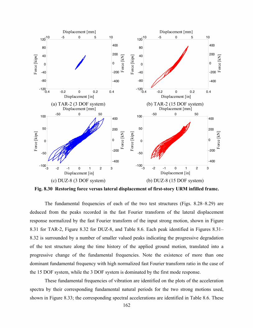
162
-0.4 -0.2 0 0.2 0.4-120
-80
-40
0
40
80
120
Displacement [in]
Forc
e [ki
ps]
-10 -5 0 5 10
-400
-200
0
200
400
Displacement [mm]
Forc
e [kN
]
-0.4 -0.2 0 0.2 0.4-120
-80
-40
0
40
80
120
Displacement [in]
Forc
e [ki
ps]
-10 -5 0 5 10
-400
-200
0
200
400
Displacement [mm]
Forc
e [kN
]
(a) TAR-2 (3 DOF system) (b) TAR-2 (15 DOF system)
-3 -2 -1 0 1 2 3-100
-50
0
50
100
Displacement [in]
Forc
e [ki
ps]
-50 0 50
-400
-200
0
200
400
Displacement [mm]
Forc
e [kN
]
-3 -2 -1 0 1 2 3-100
-50
0
50
100
Displacement [in]
Forc
e [ki
ps]
-50 0 50
-400
-200
0
200
400
Displacement [mm]
Forc
e [kN
]
(c) DUZ-8 (3 DOF system) (b) DUZ-8 (15 DOF system)
Fig. 8.30 Restoring force versus lateral displacement of first-story URM infilled frame.
The fundamental frequencies of each of the two test structures (Figs. 8.28–8.29) are
deduced from the peaks recorded in the fast Fourier transform of the lateral displacement
response normalized by the fast Fourier transform of the input strong motion, shown in Figure
8.31 for TAR-2, Figure 8.32 for DUZ-8, and Table 8.6. Each peak identified in Figures 8.31–
8.32 is surrounded by a number of smaller valued peaks indicating the progressive degradation
of the test structure along the time history of the applied ground motion, translated into a
progressive change of the fundamental frequencies. Note the existence of more than one
dominant fundamental frequency with high normalized fast Fourier transform ratio in the case of
the 15 DOF system, while the 3 DOF system is dominated by the first mode response.
These fundamental frequencies of vibration are identified on the plots of the acceleration
spectra by their corresponding fundamental natural periods for the two strong motions used,
shown in Figure 8.33; the corresponding spectral accelerations are identified in Table 8.6. These

163
spectral values are rather consistent with the observed response discussed above. This is
particularly true when taking into consideration another contributing factor to the observed
difference in response between the 3 DOF and 15 DOF systems which are the higher-mode
effects in the 15 DOF system. While the 3 DOF system is dominated by the first mode response,
shown in Figures 8.31(a) and 8.32(a), the higher modes in the 15 DOF system contribute
significantly to the response as demonstrated by the peaks observed in Figures 8.31(b) and
Figure 8.32(b).
5 10 150
0.5
1 8.21 (0.121 sec)
Nor
mal
ized
FFT
ratio
Frequency [Hz]5 10 15
0
0.5
1 8.21 (0.121 sec)
Nor
mal
ized
FFT
ratio
Frequency [Hz] (a) 3 DOF system
5 10 150
0.5
1
3.62 (0.276 sec)
7.49
9.40
Nor
mal
ized
FFT
ratio
Frequency [Hz]5 10 15
0
0.5
1
3.62 (0.276 sec)
7.49
9.40
Nor
mal
ized
FFT
ratio
Frequency [Hz] (b) 15 DOF system
Fig. 8.31 Evaluated fundamental frequencies of vibration in TAR-2 for different structural systems.

164
5 10 150
0.5
12.58 (0.388 sec)
Nor
mal
ized
FFT
ratio
Frequency [Hz]5 10 15
0
0.5
12.58 (0.388 sec)
Nor
mal
ized
FFT
ratio
Frequency [Hz] (a) 3 DOF system
5 10 150
0.5
1
3.16 (0.317 sec) 6.03
9.68
Nor
mal
ized
FFT
ratio
Frequency [Hz]5 10 15
0
0.5
1
3.16 (0.317 sec) 6.03
9.68
Nor
mal
ized
FFT
ratio
Frequency [Hz] (b) 15 DOF system
Fig. 8.32 Evaluated fundamental frequencies of vibration in DUZ-8 for different structural systems.
Table 8.6 Natural periods nT and corresponding spectral accelerations AS .
3 DOF system 15 DOF system Ratio (15 DOF / 3 DOF) Strong
Motion nT (sec)
AS (g)
nT (sec)
AS (g) AS
Peak lateral displacement
demand TAR-2 0.121 0.42 0.276 1.02 2.43 1.88 DUZ-8 0.388 2.66 0.317 3.38 1.27 0.79

165
0 0.2 0.4 0.6 0.8 10
1
2
3
4
5
6
Period [sec]
Spec
tral a
ccel
erat
ion
[g]
TAR-2DUZ-8
TAR
3 D
OF
DU
Z 3
DO
F
DU
Z 15
DO
FTA
R 1
5 D
OF
0 0.2 0.4 0.6 0.8 10
1
2
3
4
5
6
Period [sec]
Spec
tral a
ccel
erat
ion
[g]
TAR-2DUZ-8
TAR
3 D
OF
DU
Z 3
DO
F
DU
Z 15
DO
FTA
R 1
5 D
OF
Fig. 8.33 Spectral acceleration of applied strong motions (5% damping ratio) for quantifying contribution of upper stories.
8.6 TEST STRUCTURE B
The seismic response of test structure B, namely the first-story shear walls of a two-story wood
house with a garage opening in the first story is evaluated herein based on its response to three
seismic motions applied in sequence. These strong motions are LPG levels 2, 4, and 6, refer to
Tables 5.1–5.2, denoted LPG-2, LPG-4, and LPG-6, respectively, in the following discussion. A
comparison is finally made between the responses of the HS test structure B and the
corresponding ST test structure.
8.6.1 Force-Displacement Behavior
The total base shear, as defined in Section 8.1.1, is plotted versus the shear-wall lateral
displacement for the three different levels of the applied strong motion LPG. As in the case of
test structure A (see Section 8.1.1), the stiffness values in Figure 8.34 are estimated based on the
tangent slopes at different stages of the applied strong motion evaluated over a number of lading
branches using the least-squares method to obtain a best linear fit. In LPG-2 (Fig. 8.34(a)), the

166
tangent stiffness is estimated as K = 9.9 kips/in. (1.73 kN/mm) where the shear walls are still
undamaged and behave almost elastically. As the level of shaking increases to LPG-4, the nails
(fasteners) connecting the shiplap siding to the timber shear-wall framing (studs) (Fig. 8.35) are
deformed beyond their elastic ranges and induce crushing in the framing, which creates a
progressively expanding gap around the nail shank as the shear walls are cycled back and forth
(Judd and Fonseca 2005; Dinehart and Shenton 2000; White and Dolan 1995).
A great reduction in stiffness of the shear walls, to 1K = 1.9 kips/in. (0.33 kN/mm), is
observed in the range of shear-wall lateral displacement where the gaps surrounding the nail
shanks are formed and the nails are deformed. The stiffness is higher beyond that range at 2K =
5.3 kips/in. (0.93 kN/mm), resulting in the pinching behavior observed in Figure 8.34(b). Note
that at that point, the nails connecting the diagonal struts to the vertical studs are completely
pulled out (Fig. 8.36(a)). The diagonal struts are therefore ineffective in shear resistance,
contributing to a 46% reduction in stiffness, from 9.9 kips/in. (1.73 kN/mm) in LPG-2 to 5.3
kips/in. (0.93 kN/mm) in LPG-4.
The behavior described above is taken to a greater level of lateral displacement of 5.4 in.
(137 mm) in LPG-6, where the total base shear force reaches a maximum of 12.1 kips (53.8 kN)
(Fig. 8.34(c)) and slight reductions in 1K = 1.3 kips/in. (0.23 kN/mm) and 2K = 4.2 kips/in. (0.74
kN/mm) are observed. The deformation of the shear-wall shiplap siding is characterized by a
stair-like form, as shown in Figure 8.36(b), which is sustained for large lateral displacement as
observed from the long plateau in the positive large excursion of Figure 8.34(c), along with a
slight degradation of stiffness, as long as the nails are not completely pulled out of the framing
studs.

167
-3 -1.5 0 1.5 3-10
-5
0
5
10
Displacement [in]
Forc
e [ki
ps]
-50 0 50
-25
0
25
Displacement [mm]
Forc
e [kN
]
K = 9.9 kips/in
-3 -1.5 0 1.5 3-10
-5
0
5
10
Displacement [in]
Forc
e [ki
ps]
-50 0 50
-25
0
25
Displacement [mm]
Forc
e [kN
]
K = 9.9 kips/in
(a) LPG-2
-3 -1.5 0 1.5 3-10
-5
0
5
10
Displacement [in]
Forc
e [ki
ps]
-50 0 50
-25
0
25
Displacement [mm]
Forc
e [kN
] K1 = 1.9 kips/in
K2 = 5.3 kips/in
-3 -1.5 0 1.5 3-10
-5
0
5
10
Displacement [in]
Forc
e [ki
ps]
-50 0 50
-25
0
25
Displacement [mm]
Forc
e [kN
] K1 = 1.9 kips/in
K2 = 5.3 kips/in
(b) LPG-4
-6 -3 0 3 6-15
-10
-5
0
5
10
15
Displacement [in]
Forc
e [ki
ps]
-150 -100 -50 0 50 100 150
-50
-25
0
25
50
Displacement [mm]
Forc
e [kN
] K1 = 1.3 kips/in
K2 = 4.2 kips/in
-6 -3 0 3 6-15
-10
-5
0
5
10
15
Displacement [in]
Forc
e [ki
ps]
-150 -100 -50 0 50 100 150
-50
-25
0
25
50
Displacement [mm]
Forc
e [kN
] K1 = 1.3 kips/in
K2 = 4.2 kips/in
(c) LPG-6
Fig. 8.34 Total base shear versus lateral displacement for HS for test structure B (1 kip/in.=0.175 kN/mm).

168
P
Deformed nail
Undeformed nail
Framing stud
Sheathing (shiplap siding)
P
Deformed nail
Undeformed nail
Framing stud
Sheathing (shiplap siding)
Fig. 8.35 Framing-to-sheathing connection schematic of local deformation.
(a) Diagonal strut dislocation (LPG-4) (b) Stair-like deformed shape of shiplap
siding (LPG-6)
Fig. 8.36 Deformed shape of wood shear walls at peak lateral displacement.
8.6.2 Comparison to ST Experiment
The HS results discussed in Section 8.6.1 are compared to the ST experimental results in this
section, where two levels of strong motion are treated, namely, LPG-4 and LPG-6. In LPG-4
(Fig. 8.37), the same pinching behavior is observed in the ST experiment with similar estimated
tangent stiffness values as in the HS experiment. The time-history plots for lateral displacement
of the first story (Fig. 8.38) and for total base shear (Fig. 8.39) show a good match of behavior
between the HS and the ST experiments for LPG-4 motion. Note that the displacement time
histories are quite similar up to the peak recorded at 5 sec, where the HS test structure is
subjected to a slightly larger lateral displacement (in the absolute sense) compared to the ST test

169
structure (-2.35 in. (-59.7 mm) in HS versus -1.98 in. (-50.3 mm) in ST). From this point on, a
tendency of the HS test structure to deform on the negative side of the plotted displacement is
observed resulting in a residual displacement of -0.35 in. (-8.9 mm) at the end of the strong
motion.
-3 -1.5 0 1.5 3-10
-5
0
5
10
Displacement [in]
Forc
e [k
ips]
-50 0 50
-25
0
25
Displacement [mm]
Forc
e [k
N] K1 = 1.9 kips/in
K2 = 5 kips/in
Fig. 8.37 Total base shear versus first-story lateral displacement for test structure B for LPG-4 (ST experiment).
In LPG-6, the responses once more show a similarity between the HS and the ST
experiments in terms of the lateral displacement pattern of the first story and period of vibration
(Fig. 8.40), as well as in the total base shear (Fig. 8.41). In the HS experiment, however, the test
structure is left with a larger residual displacement of 1.84 in. (46.7 mm), while the ST test
structure almost returns to the zero displacement position as observed in the previous level of
LPG-4. Note that in the HS experiment, the actuator is locked at the last reached displacement
position in the applied strong motion, while in the ST experiment, the test structure is left to
vibrate freely and any tendency of the test structure to return to its original position is not
restrained. This tendency may have substantial effects in terms of the recorded residual
deformation in both experiments. This observation is particularly amplified, since the stiffness of
the damaged test structure at the origin is very low (1.3 kips/in. (0.23 kN/mm)) in the case of
LPG-6 in HS (Fig. 8.34(c)), i.e., a small amplitude force of 1 kip (4.45kN) may cause the shear
walls to deform more than 0.75 in. (19 mm).

170
0 5 10 15 20-3
-2
-1
0
1
2
3
Disp
lace
men
t [in
]
-150
-100
-50
0
50
100
150
Disp
lace
men
t [m
m]HS
0 5 10 15 20-3
-2
-1
0
1
2
3
Time [sec]
Disp
lace
men
t [in
]
-150
-100
-50
0
50
100
150
Disp
lace
men
t [m
m]ST
Fig. 8.38 Displacement time-history comparison for test structure B for LPG-4.
0 5 10 15 20-10
-5
0
5
10
Bas
e sh
ear [
kips
] HS
-25
0
25
Bas
e sh
ear [
kN]
0 5 10 15 20-10
-5
0
5
10
Time [sec]
Bas
e sh
ear [
kips
] ST
-25
0
25B
ase
shea
r [kN
]
Fig. 8.39 Total base shear time-history comparison for test structure B for LPG-4.

171
0 10 20 30 40-6
-4
-2
0
2
4
6
Disp
lace
men
t [in
]
-150
-100
-50
0
50
100
150
Disp
lace
men
t [m
m]HS
0 5 10 15 20 25 30 35 40 45-6
-4
-2
0
2
4
6
Time [sec]
Disp
lace
men
t [in
]
-150
-100
-50
0
50
100
150
Disp
lace
men
t [m
m]ST
Fig. 8.40 Displacement time-history comparison for test structure B for LPG-6.
0 10 20 30 40-15
-10
-5
0
5
10
15
Bas
e sh
ear [
kips
] HS
-50
-25
0
25
50
Bas
e sh
ear [
kN]
0 10 20 30 40-15
-10
-5
0
5
10
15
Time [sec]
Bas
e sh
ear [
kips
] ST
-50
-25
0
25
50B
ase
shea
r [kN
]
Fig. 8.41 Total base shear time-history comparison for test structure B for LPG-6.
Moreover, the HS test structure is simulated as a SDOF system, and the contribution of
the higher modes (particularly the second flexural mode of vibration of the two-story ST test
structure) to the structural response of the HS test structure are completely neglected. This

172
contribution, in the case of the ST experiment, is capable of counteracting the fundamental
modal response (first flexural mode of vibration of the two-story ST test structure); resulting in
minimizing the residual displacement of the test structure. However, after a number of repeated
runs (repeating LPG-1, LPG-2, LPG-3, LPG-4, and LPG-6, Tables 5.1–5.2, each three times)
applied on the ST test structure, the accumulation of damage results in a modest residual
displacement of 0.93 in. (23.6 mm), as shown in Figure 8.42, for the last repeat of LPG-6.
0 5 10 15 20 25 30 35 40 45 50-10
-5
0
5
10
Time [sec]
Disp
lace
men
t [in
]
-200
-100
0
100
200
Disp
lace
men
t [m
m]
Fig. 8.42 Displacement time-history for test structure B for third (last) repetition of LPG-6 (ST experiment).
8.7 SUMMARY
This chapter presents the results of phases S-1, S-2, and S-3 of test structure A (see Fig. 1.2), in
addition to the structural evaluation of test structure B. Novel comparisons to the corresponding
shaking table experiments for each phase are discussed. The main results and inferred
conclusions are summarized in the following list: • In phase S-1, the global response represented by the total base shear of test structure A
versus the lateral displacement is illustrated, and the deterioration of the test structure is
monitored in terms of its estimated stiffness. • The URM infill wall contribution to the base shear resistance of test structure A is
evaluated, and the degradation of this wall in terms of the reduction of its shear
contribution and the formation of the cracking pattern is monitored. • The results of phase S-1 of test structure A are compared to the shaking table experiment,
which is conducted on a similar test structure with the same sequence of applied ground
motions.

173
• The cracking pattern and progressive degradation of test structure A throughout the two
experiments using HS and ST are compared and are found to be closely matching. • Differences due to the rate of load application of the HS and ST experiments are
observed leading to a difference in the nature of the sliding mechanism at the interface
between the URM infill wall and the surrounding RC frame in test structure A. It is
argued that this difference in the sliding mechanism is the cause for the apparent high
initial stiffness in the HS experiment, which is absent in the ST experiment. • Other differences between HS and ST experiments for test structure A are due to the lack
of an accurate comprehensive numerical model for the viscous damping in HS. While the
damping ratio is estimated in the case of the HS test structure as a constant value based
on snap-back test results conducted on the undamaged ST test structure, the results from
the ST experiment reveal a changing damping ratio at different states of degradation of
the test structure. • Phases S-2 and S-3 for test structure A are discussed in terms of global behavior, damage
observed in the test structure, and local beam-to-column and column-to-footing joint
rotations. • The comparison between the HS experiment and the corresponding ST experiment for
test structure A, in phases S-2 and S-3, shows smaller lateral displacement in the HS
experiment due to the post-tensioning of the RC beams of the HS test structure leading to
limited damage in the beam-to-column joints. • The effect of the upper stories in a hypothetical five-story test structure on the seismic
response of test structure A is examined and the URM infilled RC frame is numerically
modeled using the nonlinear hysteretic Bouc-Wen model. • The difference in the fundamental frequency between the one-story and five-story test
structures as well as the participation of higher modes in the case of the five-story
structure are found to have a significant effect on the structural response of test structure
A. • The global response of test structure B is evaluated revealing the familiar pinching
behavior and stair-like deformation of the timber shear walls with shiplap siding. • The corresponding ST experimental results, compared to those of the HS of test structure
B, reasonably match in terms of the general global response and magnitudes of lateral
displacement and total base shear.

174
• For test structure B, a major difference is observed between the HS and the ST
experiments in terms of the residual displacement, which is larger in the case of the HS
experiment. This is attributed to the differences in boundary conditions of the HS and ST
test structures and to the absence of the higher-mode contribution to the response in the
HS experiment where the test structure is simulated as a SDOF system.

9 Summary, Conclusions, and Future Work
9.1 SUMMARY
The hybrid simulation system (HSS) of the University of California, Berkeley (UCB), namely
nees@berkeley, is fully utilized and expanded in the present study, which also identifies the main
components of the system and the interconnections defining its functionality. A validation
experiment is carried out for the purpose of ensuring the proper functionality of the newly
installed system. This experiment is developed as two coupled steel cantilevers in which one
behaves linearly and the other behaves bilinearly with increasing stiffness by means of a stiffener
with an adjustable gap. The experiment is designed with a numerically reproducible structural
behavior of the test specimens in which experimental results using the HSS are validated against
pure numerical simulation.
Two test structures are used in this study, namely reinforced concrete (RC) frames with
and without unreinforced masonry (URM) infill walls, test structure A discussed in Chapter 4,
and a two-story wood house including an open first-story garage, test structure B discussed in
Chapter 5. The structural performance of the two test structures under seismic loading is
examined. These two test structures have the common feature of being large substructures of
shaking table (ST) experiments conducted at UCB for different structural systems. Novel
comparisons are therefore conducted between the HS results for each of these test structures with
the results from its corresponding counterpart on the ST, with the aim of stating the similarities
and identifying the sources of discrepancy between the results of the two testing methods.
Two novel procedures, namely feed-forward error compensation and mixed-variables
control are developed and implemented in the HSS. The first procedure leads to a more accurate
execution of the displacement command signal. The second procedure uses mixed
displacement/force control for flexible/stiff (hybrid) structural systems, offering a valuable

176
solution for testing such hybrid systems pseudo-dynamically. In summary, the study is successful
in developing significant steps toward a generalized framework for hybrid simulation to be
successfully conducted on structural systems, including hybrid ones, subjected to seismic loading
with detailed validations using ST experimentation.
9.2 CONCLUSIONS
The following list summarizes the main conclusions inferred from the present study: • The validation experiment confirms the proper functionality of the HSS used in the
present study, including the implementation of the numerical-integration algorithm used
in displacement control. • The structural dynamic response of the one-story RC frame structure with and without
URM infill wall, phase S-1 in Figure 1.2, is dominated by the high stiffness offered by
the URM infill wall, and therefore such a wall provides more than 80% of the lateral total
base shear resistance in the undamaged state. This contribution decreases as the URM
infill wall degrades and reaches only 9% of the total base shear resistance at the end of
phase S-1 where several levels of ground motion are applied to the test structure up to the
in-plane collapse of the URM infill wall with severe shaking. • In phases S-2 and S-3 in Figure 1.2, for the one-story test structure after the removal of
the URM infill wall, the RC frame structure undergoes large lateral displacement,
reaching 6.5% lateral story drift at the end of phase S-3. The damage and joint rotations
are concentrated in the column-to-footing joints, whereas the beam-to-column joints do
not undergo major damage, which is attributed to the post-tensioning of the RC beams for
HS loading purposes protecting the top column joints as well as to the seismic detailing
of these joints. • The wood shear walls with shiplap siding in test structure B lose 46% of their initial
stiffness after the application of the first strong motion (at 25% upper-bound earthquake,
i.e., 10% probability of exceedance in 100 years) due to the dislocation of the diagonal
struts between the studs of the shear walls. • The nails connecting the shiplap siding to the vertical studs of test structure B control the
response of the structure after loosening of the diagonal struts. The test structure has a
very low lateral stiffness in the lateral displacement range where the framing fibers are

177
crushed around the nail shanks, while holding most of its stiffness beyond that range
resulting in a pinching bilinear behavior with high unloading stiffness. This behavior is
maintained throughout the applied sequence of strong motions, justifying the use of a
testing approach with force control. • In test structure A, the comparison of the HS experimental results to its counterpart from
the ST experiment reveals that the slow execution of the HS experiment (80 times slower
than real time) causes the nature of the sliding mechanism at the interface between the
URM infill wall and the surrounding RC frame to differ, leading to higher apparent
stiffness in the HS experiment. • Other differences between the HS and the ST experiments are due to the lack of an
accurate comprehensive numerical model for the viscous damping in HS. The damping
ratio is estimated as constant in this study based on snap-back test results conducted on
the undamaged ST test structure, while results from the ST experiment (Hashemi and
Mosalam 2007) reveal a changing damping ratio at different states of degradation of the
test structure. • A study of the upper stories effect in the case of test structure A underlines the
importance of considering the higher modes in the dynamic response of the test structure.
While it is practically very difficult to consider that effect in the ST experiment,
numerical substructuring in HS offers this possibility. This conclusion is also confirmed
in the comparison of the HS and ST experiments performed on test structure B. • The error in executing the displacement command signal in displacement-controlled HS
is predicted based on a calibrated hockey-stick model, and a feed-forward error
compensation scheme is implemented within the HSS leading to a more accurate
execution of the HS experiment. • A novel implicit force-control algorithm is developed and a parametric study confirms its
accuracy. • A mixed-variables control procedure is implemented within the HSS, and a number of
implementation strategies are developed to ensure the smooth functionality of the
procedure and to allow the mode switch between displacement and force control to be
performed accurately and practically.

178
• The implementation of the mixed-variables control procedure on test structure A revealed
the need for proper actuator tuning in force control for the success of the developed
procedure. • The implementation of the mixed-variables control procedure on test structure B
validates its proper implementation and functionality within the HSS.
9.3 FUTURE WORK
The following list summarizes the suggested topics based on the conducted study where further
research is needed: • The implementation of the mixed-variables procedure is proven to be useful in the case of
flexible/stiff structures. However, actuator control tuning parameters are stiffness
dependent; therefore, in order for the HSS to be able to implement force control in a wide
range of stiffness of the test structure, it needs to allow online adjustments to these
parameters during the experiment, which was not available during this study. The
exploration of that option may render mixed-variables control more useful in testing a
larger variety of structures over a wider range of their seismic response. • In the feed-forward error compensation procedure, the online estimation of the hockey-
stick model parameters would allow the error prediction and compensation to be
implemented during the same test run, which would alleviate the need for a separate run
for the purpose of calibration and would also make the procedure suitable for situations
where these parameters may change during testing. This is an important endeavor to be
pursued in future enhancements of the developed generalized framework for the HS in
this report. • Macro-element modeling allows the numerical modeling of complex structural elements,
such as the URM infilled RC frame simulated in this study using the Bouc-Wen model.
Such models can be used in parametric studies, within the generalized framework for the
HS developed in this report, offering the possibility of studying important problems such
as evaluating the effect of the amount of numerical damping and its different modeling
assumptions on the dynamic response of complex structural systems. • In this study, test structure A was excited by unidirectional ground motions parallel to the
plane of the RC frames and the URM infill wall. However, the contribution of out-of-

179
plane excitation forces to the structural performance of the test structure is of great
importance. Although a three-dimensional finite element computational model was
developed in Hashemi and Mosalam (2007) to study this out-of-plane contribution, an
experimental study should be conducted, using the developed generalized framework for
HS in this report, to reach a better understanding of this important problem. • The RC frames in test structure A are seismically detailed and a HS experimental study is
needed to evaluate the dynamic response of the very common worldwide non-seismically
detailed (gravity-load designed) RC frame structures with and without URM infill walls.
Moreover, the developed HSS will offer an excellent platform on which to develop
possible retrofit schemes for URM infill walls and their bounding seismically deficient
RC frames.

181
References
ACI Committee 318. 2002. Building code requirements for structural concrete (ACI 318-02) and
commentary (ACI 318R-02). American Concrete Institute.
ASTM C837-99. 1999. Standard test method for compressive strength of concrete cylinders cast-
in-place in cylindrical molds. ASTM, West Conshohocken, PA.
ASTM C270-03. 2003. Standard specification for mortar for unit masonry. ASTM, West
Conshohocken, PA.
ASTM C1314-02a. 2002. Standard test method for compressive strength of masonry prisms.
ASTM, West Conshohocken, PA.
Baber, T.T. and Wen, Y.K. 1981. Random vibration of hysteretic, degrading Systems. Journal of
the Engineering Mechanics Division, ASCE 107(EM6): 1069-1087.
Baber, T.T. and Noori, M.N. 1986. Modeling general hysteresis behavior and random vibration
application. Journal of Vibration, Acoustics, Stress, and Reliability in Design 108(October):
411-420.
Bonelli, A. and Bursi O.S. 2004. Generalized-α methods for seismic structural testing.
Earthquake Engineering and Structural Dynamics 33(10): 1067-1102.
Building Seismic Safety Council (BSSC). 2000. NEHRP recommended provisions for seismic
regulations for new buildings and other structures. Part 1: Provisions (FEMA368) and Part
2: Commentary (FEMA369), Washington D.C.
Buonopane, S.G. 1997. Seismic evaluation of a masonry infilled reinforced concrete frame by
pseudodynamic testing. M.Sc. Thesis, School of Civil and Environmental Engineering,
Cornell University, Ithaca, New York.
Chopra, A.K. 2000. Dynamics of structures: theory and applications to earthquake engineering.
Second Edition, Prentice Hall, Inc., Upper Saddle River, New Jersey.
Darby, A.P., Blakeborough, A. and Williams, M.S. 2001. Improved control algorithm for real-

182
time substructure testing. Earthquake Engineering and Structural Dynamics 30(3): 431-448.
Dermitzakis, S.N. and Mahin, S.A. 1985. Development of substructuring techniques for on-Line
computer controlled seismic performance testing. UBC/EERC-85/04, Earthquake
Engineering Research Center, University of California, Berkeley.
Dimig, J., Shield, C., French, C., Bailey, F. and Clark, A. 1999. Effective force testing: a method
of seismic simulation for structural testing. Journal of Structural Engineering, ASCE 125(9):
1028-1037.
Dinehart, D. W. and Shenton, H.W.III 2000. Model for dynamic analysis of wood frame shear
walls. Journal of Engineering Mechanics, ASCE, 126(9): 899–908.
Elkhoraibi, T. and Mosalam, K.M. 2007. Towards error-free hybrid simulation using mixed
variables. Earthquake Engineering and Structural Dynamics in press.
Fenves, G.L., McKenna, F., Scott, M.H. and Takahashi, Y. 2004. An object-oriented software
environment for collaborative network simulation. Proceedings, 13th World Conference on
Earthquake Engineering, Vancouver, Canada.
Gawthrop, P.J., Wallace, M.I. and Wagg, D.J. 2005. Bond-graph based substructuring of
dynamical systems. Earthquake Engineering and Structural Dynamics 34(6): 687-703.
Hanson, R.D. and McClamroch, N.H. 1984. Pseudodynamic test method for inelastic building
response. Proceedings of the 8th World Conference in Earthquake Engineering, San
Francisco.
Hashemi, A. and Mosalam, K.M. 2007. Seismic evaluation of reinforced concrete buildings
including effects of masonry infill walls. PEER Report 2007/100. Pacific Earthquake
Engineering Research Center, Department of Civil and Environmental Engineering,
University of California, Berkeley.
Hashemi, A. and Mosalam, K.M. 2006. Shake-table experiment on reinforced concrete structure
containing masonry infill wall. Earthquake Engineering and Structural Dynamics 35(14):
1827-1852.
Hilber, H., Hughes, T. and Taylor, R. 1977. Improved numerical dissipation for time integration
algorithms in structural dynamics. Earthquake Engineering and Structural Dynamics 5(3):
283-292.
Hughes T.J.R. 1983. Analysis for transient algorithms with particular reference to stability
behavior. Computational Methods for Transient Analysis Belyschko, T. and Hughes, T.J.R.,
Editors, Amsterdam, North-Holland.

183
Hughes, T.J.R., Pister, K.S. and Taylor, R.L. 1979 Implicit-explicit finite elements in nonlinear
transient analysis. Computer Methods in Applied Mechanics and Engineering, 17/18(Part 1):
159-182.
Judd, J.P. and Fonseca, F.S. 2005. Analytical model for sheathing-to-framing connections in
wood shear walls and diaphragms. Journal of Structural Engineering, ASCE (131)2: 345-
352.
Kron, G. 1963. Diakoptics; the piecewise solution of large-scale systems. MacDonald, London,
UK, pp.166.
Magonette, G. 2001. Development and application of large-scale continuous pseudo-dynamic
testing techniques. Philosophical Transactions of the Royal Society A: Mathematical,
Physical and Engineering Sciences 359(1786): 1771-1799.
Mahin, S.A., Shing, P.B., Thewalt, C.R. and Hanson, R.D. 1989. Pseudodynamic test method –
current status and future direction. Journal of Structural Engineering, ASCE 115(8): 2113-
2128.
Mazzoni, S., McKenna, F., Scott, M.H. and Fenves, G.L. 2006. Open system for earthquake
engineering simulation user command-language manual. Pacific Earthquake Engineering
Research Center, University of California, Berkeley, Version 1.7.3, September.
McClamroch, N.H., Serakos, J. and Hanson, R.D. 1981. Design and analysis of the
pseudodynamic test method. UMEE 81R3, University of Michigan, Ann Arbor.
Menegotto M. and Pinto P.E. 1973. Method of analysis for cyclically loaded R.C. plane frames
including change in geometry and non-elastic behavior of elements under combined normal
force and bending. Proceedings of IABSE Symposium on Resistance and Ultimate
Deformability of Structures Acted on by Well Defined Repeated Loads, Lisbon 13: 15-22.
Mosalam, K.M. 1996a. Experimental and computational strategies for the seismic behavior
evaluation of frames with infill walls. PhD Dissertation, School of Civil and Environmental
Engineering, Cornell University, Ithaca, New York.
Mosalam, K.M. 1996b. Modeling of the nonlinear seismic behavior of gravity load designed
frames. Earthquake Spectra 12(3): 479-492.
Mosalam, K.M., Ayala, G. and White, R.N. 1997a. Development of fragility curves: masonry
infill-concrete frame buildings. Chapter 7 of Technical Report NCEER-97-0018, Loss
Assessment of Memphis Buildings, D.P. Abrams and M. Shinozuka (Eds.).

184
Mosalam, K.M., White, R.N. and Gergely, P. 1997b. The seismic evaluation of frames with infill
walls using quasi-static experiments. Technical Report NCEER-97-0019.
Mosalam, K.M., White, R.N. and Gergely, P. 1997c. The seismic evaluation of frames with infill
walls using pseudodynamic experiments. Technical Report NCEER-97-0020.
Mosalam, K.M., White, R.N. and Gergely, P. 1997d. Static response of infilled frames using
quasi-static experimentation. Journal of Structural Engineering, ASCE 123(11): 1462-1469.
Mosalam, K.M., Ayala, G., White, R.N. and Roth, C. 1997e. Seismic fragility of LRC frames
with and without masonry infill walls. Journal of Earthquake Engineering 1(4): 693-720.
Mosalam, K.M., White, R.N. and Ayala, G. 1998. Response of infilled frames using
pseudodynamic experimentation. Earthquake Engineering and Structural Dynamics 27(6):
589-608.
Mosalam, K.M., Machado, C., Gliniorz, K.-U., Naito, C., Kunkel, E. and Mahin, S. 2002.
Seismic evaluation of asymmetric three-story wood-frame building. CUREE Publication No.
W-19.
Mosalam, K.M. and Mahin, S.A. 2007. Seismic evaluation and retrofit of asymmetric multi-story
wood-frame building. Journal of Earthquake Engineering, in press.
Mosalam, K.M. and Elkhoraibi, T. 2004. RRW system: specifications, usage and training
example http://nees.berkeley.edu/Facilities/rrw.shtml
Mosqueda G. 2003. Continuous hybrid simulation with geographically distributed substructures.
PhD Dissertation, Department of Civil and Environmental Engineering, University of
California, Berkeley.
MTS. 2003. Model 793.00 System software, user information and software reference. MTS
Systems Corporation.
Nakashima, M. 2001. Development, potential, and limitations of real-time online (pseudo-
dynamic) testing. Philosophical Transactions of the Royal Society A: Mathematical, Physical
and Engineering Sciences 359(1786): 1851–1867.
Nakashima, M., Kaminosono, T., Ishida, M. and Ando, K. 1990. Integration techniques for
substructure pseudodynamic testing. Proceedings of the 4th U.S. National Conference on
Earthquake Engineering, Palm Springs, California II: 515-524.
Nakashima, M. and Masaoka, N. 1999. Real-time on-line test for MDOF systems. Earthquake
Engineering and Structural Dynamics 28(4): 393-420.

185
Newmark N.M. 1959. A Method of Computation for structural dynamics. Journal of
Engineering Mechanics Division, ASCE 85(EM3): 67-94.
Pacific Instruments. 2004. PI660-6000, version 8.0, operator’s manual. Pacific Instruments
Corporation.
Pan, P. 2004. Safety and functionality of base-isolated building structures subjected to vertical
ground motions. PhD Dissertation, Kyoto University, Japan.
Pan, P., Nakashima, M. and Tomofuji, H. 2005. Online test using displacement–force mixed
control. Earthquake Engineering and Structural Dynamics 34(8): 869-888.
Pan P., Tomofuji H., Wang T., Nakashima M., Ohsaki M. and Mosalam, K.M. 2006.
Development of peer-to-peer (P2P) internet online hybrid test system. Earthquake
Engineering and Structural Dynamics 35(7): 867–890.
Pinto, A., Pegon, P., Magonette, G., Molina, J., Buchet, P. and Tsionis G. 2002. Pseudodynamic
tests on a large-scale model of an existing RC bridge using non-linear substructuring and
asynchronous motion. EUR 20525 EN, European Laboratory for Structural Assessment,
Ispra, Italy.
Schellenberg, A., Mahin, S. and Fenves, G. 2007. A software framework for hybrid simulation of
large structural systems. Proceedings of Structures Congress, ASCE, Reston, VA, 1269.
Seible, F., Hegemier, G.A., Igarashi, A. and Kingsley, G.R. 1994a. Simulated seismic-load tests
on full-scale five-story masonry building. Journal of Structural Engineering, ASCE 120(3):
903-924.
Seible, F., Priestley, M.J.N., Kingsley, G.R. and Kürkchübasche, A.G. 1994b. Seismic response
of full-Scale five story reinforced-masonry building. Journal of Structural Engineering,
ASCE 120(3): 925-946.
Seible, F., Hegemier, G.A. and Igarashi, A. 1996. Simulated seismic laboratory load testing of
full-scale buildings. Earthquake Spectra, EERI 12(1): 57-86.
Shield, C., French, C. and Timm, J. 2001. Development and implementation of the effective
force testing method for seismic simulation of large-scale structures. Philosophical
Transaction of the Royal Society A: Mathematical, Physical and Engineering Sciences
359(1786): 1911-1929.
Shing, P.B., Javadian-Gilani, A.S. and Mahin, S.A. 1984. Evaluation of seismic behavior of a
braced tubular steel structure by pseudodynamic testing. Journal of Energy Resources
Technology, ASME Transactions 106(September): 319-328.

186
Shing P.B. and Mahin, S.A. 1983. Experimental error propagation in pseudodynamic testing.
UBC/EERC-83/12, Earthquake Engineering Research Center, University of California,
Berkeley.
Shing P.B. and Mahin, S.A. 1984. Pseudodynamic test method for seismic performance
evaluation: Theory and Implementation. UBC/EERC-84/01, Earthquake Engineering
Research Center, University of California, Berkeley.
Shing, P.B. and Mahin, S.A. 1985. Computational aspects of a seismic performance test method
using on-line computer control. Earthquake Engineering and Structural Dynamics 13(4):
507-526.
Shing, P.B. and Mahin, S.A. 1987a. Cumulative experimental errors in pseudodynamic tests.
Earthquake Engineering and Structural Dynamics 15(4): 409-424.
Shing, P.B. and Mahin, S.A. 1987b. Elimination of spurious higher-mode response in
pseudodynamic tests. Earthquake Engineering and Structural Dynamics 15(4): 425-445.
Shing, P.B., Vannan, M.T. and Cater, E. 1991. Implicit time integration for pseudodynamic tests.
Earthquake Engineering and Structural Dynamics 20(6): 551-576.
Shing, P.B. Nakashima, M. and Bursi, O.S. 1996. Application of pseudodynamic test method to
structural research. Earthquake Spectra 12(1): 29-56.
Song, J. and Der Kiureghian, A. 2006. Generalized Bouc-Wen model for highly asymmetric
hysteresis. Journal of Engineering Mechanics, ASCE 132(6): 610-618.
Systran. 2000. ScramNet+ technical description. Systran Corporation.
Takahashi, Y. and Fenves, G.L. 2006. Software framework for distributed experimental-
computational simulation of structural systems. Earthquake Engineering and Structural
Dynamics 35(3): 267-291.
Takanashi, K. and Nakashima, M. 1987. Japanese activities on on-line testing. Journal of
Engineering Mechanics, ASCE 113(7): 1014-1032.
Takanashi, K., Udagawa, K., Seki, M., Okada, T. and Tanaka, H. 1975. Nonlinear earthquake
response analysis of structures by computer-actuator on-line system. Bulletin of Earthquake
Resistant Structure Research Center, No.8, Institute of Industrial Science, University of
Tokyo, Japan: 1-17.
Talaat, M., and Mosalam, K.M. Computational modeling of progressive collapse in reinforced
concrete frame structures. PEER Report 2007/xx (forthcoming). Pacific Earthquake

187
Engineering Research Center, Department of Civil and Environmental Engineering,
University of California, Berkeley.
Thewalt, C.R. and Mahin, S.A. 1987. Hybrid solution technique for generalized pseudodynamic
testing. UBC/EERC-87/09, Earthquake Engineering Research Center, University of
California, Berkeley.
Thewalt, C.R. and Mahin, S.A. 1995. An unconditionally stable hybrid pseudodynamic
algorithm. Earthquake Engineering and Structural Dynamics 24(5): 723-731.
Wang, Y.P., Lee, C.L. and Yo, T.H. 2001. Modified state-space procedures for pseudodynamic
testing. Earthquake Engineering and Structural Dynamics 30(1) 59-80.
Weaver, W.Jr., Timoshenko, S.P. and Young, D.H. 1990. Vibration problems in engineering.
Fifth edition, John Wiley & Sons.
Wen, Y.K. 1976. Method for random vibration of hysteretic systems. Journal of the Engineering
Mechanics Division 102(EM2): 249-265.
White, M.W. and Dolan, J.D. 1995. Nonlinear shear-wall analysis. Journal of Structural
Engineering, ASCE 121(11): 1629–1635.
Wiberg, N.E. 1974. Matrix structural analysis with mixed variables. International Journal of
Numerical Methods in Engineering 8(11) 167-194.
Wu, B., Wang, Q., Shing, P.B. and Ou, J. 2007. Equivalent force control method for generalized
real-time substructure testing with implicit integration. Earthquake Engineering and
Structural Dynamics in press.
Yamazaki, Y., Nakashima, M. and Kaminosono, T. 1989. Reliability of pseudodynamic test in
earthquake response simulation. Journal of Structural Engineering, ASCE 115(8): 2098-
2112.

189
Appendix A: Spreadsheet for Configuring the Reaction Wall
A.1 BACKGROUND
A spreadsheet is developed to estimate the governing parameters of the reconfigurable reaction
wall (RRW). A fixed-base condition is assumed throughout the spreadsheet calculations. The
user provides a number of inputs to define the RRW configuration and the conditions of its use.
These inputs are: • Reaction wall height (number of RRW units) • Number of post-tensioning rods used per reaction wall (typically 10) • Post-tensioning force applied per rod (typically 100 kips) • Loading direction with respect to the reaction wall axes (weak or strong axis)
In the case where a second reaction wall is used adjacent to the first reaction wall for
increased stiffness and load-carrying capacity, the same four previous inputs are provided for the
second reaction wall, in addition to: • Position of the second reaction wall with respect to the first reaction wall (side by side or
back to back) • The user also provides: • Deflection limit for the RRW • Tension stress limit
Material parameters such as unit mass, concrete and steel strength and stiffness (elastic
moduli), and the coefficient of friction at the interface of the reaction wall units, are also
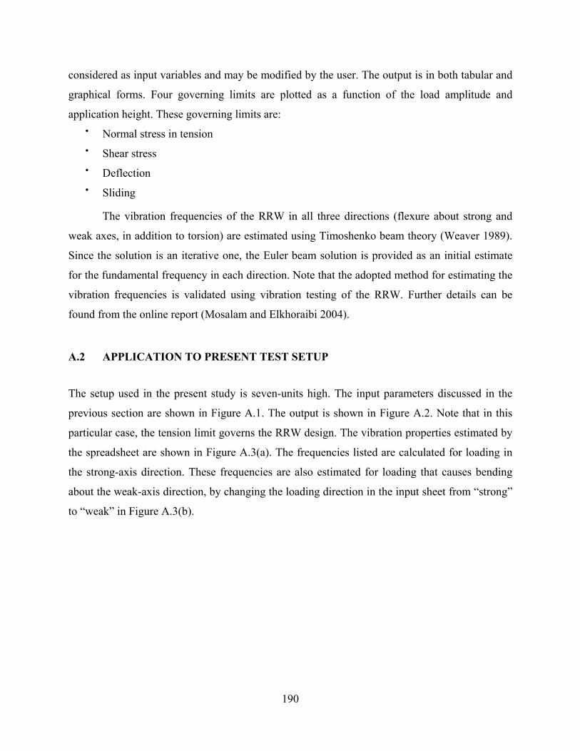
190
considered as input variables and may be modified by the user. The output is in both tabular and
graphical forms. Four governing limits are plotted as a function of the load amplitude and
application height. These governing limits are: • Normal stress in tension • Shear stress • Deflection • Sliding
The vibration frequencies of the RRW in all three directions (flexure about strong and
weak axes, in addition to torsion) are estimated using Timoshenko beam theory (Weaver 1989).
Since the solution is an iterative one, the Euler beam solution is provided as an initial estimate
for the fundamental frequency in each direction. Note that the adopted method for estimating the
vibration frequencies is validated using vibration testing of the RRW. Further details can be
found from the online report (Mosalam and Elkhoraibi 2004).
A.2 APPLICATION TO PRESENT TEST SETUP
The setup used in the present study is seven-units high. The input parameters discussed in the
previous section are shown in Figure A.1. The output is shown in Figure A.2. Note that in this
particular case, the tension limit governs the RRW design. The vibration properties estimated by
the spreadsheet are shown in Figure A.3(a). The frequencies listed are calculated for loading in
the strong-axis direction. These frequencies are also estimated for loading that causes bending
about the weak-axis direction, by changing the loading direction in the input sheet from “strong”
to “weak” in Figure A.3(b).

191
Fig. A.1 Design spreadsheet input for RRW design.

192
221
0.0
5.0
10.0
15.0
20.0
0 100 200 300 400 500 600 700 800 900 1000 1100 1200
Actuator load [kip]
Hei
gth
[ft]
tension limit shear limit displacement limit sliding limit
Fig. A.2 Design spreadsheet output for used RRW (1 kip = 4.448 kN, 1 ft = 30.48 mm).
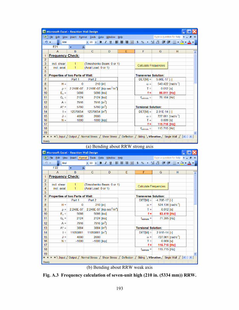
193
(a) Bending about RRW strong axis
(b) Bending about RRW weak axis
Fig. A.3 Frequency calculation of seven-unit high (210 in. (5334 mm)) RRW.

195
Appendix B: Exact Solution for a Bilinear Stiffening SDOF
In the numerical study of the mixed-variables control integration algorithm in Section 6.5.3, the
response of a bilinear stiffening elastic undamped SDOF system (Fig. B.1 (a)), is considered
when subjected to a constant impulse force op (Fig. B.1(b)).
Ik
Sk
pu
SI k,k
m ( )tp
Res
torin
g fo
rce,
R
uDisplacement,
Ik
Sk
pu
SI k,k
m ( )tp
Res
torin
g fo
rce,
R
uDisplacement, uDisplacement, 0 0.5 10
1
2
Time
App
lied
forc
e
op
0 0.5 10
1
2
Time
App
lied
forc
e
op
(a) Bilinear elastic element (b) Applied constant impulse force
Fig. B.1 Considered SDOF system.
Given the amplitude of the constant impulse force op (Fig. B.1(b)), and the deformation
pu (Fig. B.1(a)) at which the stiffness of the bilinear spring element changes from the initial
stiffness Ik to the secondary stiffness Sk , the displacement of the SDOF system at any time t
can be described by:
( ) ( ) ( )[ ]{ } ( )[ ] ( )[ ]
( ) ( ) ( )[ ]{ } ( )[ ] ( )[ ] plastIS
S
lastIlast
ISlastI
lastISSst
plastSI
I
lastSlast
SIlastS
lastSIIst
uuttuttuttutu
uuttuttuttutu
>−+−+−−=
≤−+−+−−=
ωω
ωω
ωω
ωω
sincoscos1
sincoscos1 (B.1)

196
where the subscripts I and S refer to “Initial” and “Secondary,” respectively, ( )I
oIst k
pu = and
( ) ( ) SpIopSst kukpuu −+= , mkII =ω and mkSS =ω . The superscript last designates the
last attained displacement u or time t before the change of stiffness occurs. At the beginning of
the displacement time history 0=lastu and 0=lastt , while from the point where the displacement
reaches pu for the first time, plastS
lastI uuu == . The velocity u of the SDOF system at any time t
is governed by:
( ) ( ) ( )[ ] ( )[ ] ( )[ ]
( ) ( ) ( )[ ] ( )[ ] ( )[ ] plastIS
S
lastIlast
ISlastI
lastISSstS
plastSI
I
lastSlast
SIlastS
lastSIIstI
uuttuttuttutu
uuttuttuttutu
>⎭⎬⎫
⎩⎨⎧
−+−−−=
≤⎭⎬⎫
⎩⎨⎧
−+−−−=
ωω
ωωω
ωω
ωωω
cossinsin
cossinsin (B.2)
An example of the resulting displacement time history of this SDOF using the above closed-form
solution is illustrated in Figure B.2 with the parameters listed in Table B.1.
0 0.5 10
0.5
1
Time
Nor
mal
ized
disp
lace
men
t
Fig. B.1 Typical displacement response of bilinear stiffening undraped SDOF system.
Table B.1 Parameters for bilinear stiffening undamped SDOF system.
Parameter m Ik IS kk 5= op pu II kmT π2= Example 1 24π 220π π4 0.1 1

197
Appendix C: Bouc-Wen Model Description and Calibration
The Bouc-Wen numerical model (Wen 1976; Baber and Wen 1981; Baber and Noori 1986) is
chosen for its versatility and flexibility in simulating the structural response of nonlinear
hysteretic behavior of the type exerted by the URM infilled RC frame (see Section 8.5). The
following is a discussion of the model and the parameters that control it. The calibration of these
parameters is discussed next with its application on the URM infilled RC frame used in test
structure A for two different states of damage.
C.1 DESCRIPTION
The Bouc-Wen model is governed by a number of parameters each of which controls one or
more of its features. These parameters are: • α : may be regarded as the ratio between the hardening and elastic stiffness of the
simulated structure; • β and γ : depending on their numerical sum and difference, the model is softening or
hardening; • n : controls the sharpness of transition from the elastic to the secondary stiffness
(hardening or softening); • dt : is an arbitrary time step and should be chosen to ease any numerical ill-conditioning
in the computations; • νδ : is a degradation parameter controlling the hysteretic force without affecting the
stiffness; and • ηδ : is another degradation parameter affecting both the hysteretic force and the stiffness.

198
Additional parameters are included to introduce pinching in the model as shown in the
example in Figure C.1, generated using the parameters in Table C.1. These additional parameters
are: • 0ψ : controls the initial slack, i.e., the range of displacement around the origin with a
reduction in stiffness due to pinching; • ψδ : is a slack growth parameter; and
• ξ : determines the level of pinching, i.e., the amount of stiffness reduction in the slack
region.
The model may be described by the differential equations below:
( )
( ) ( )
( )( )
( )( ) ( )
dtdy
dtdu
Δ+δψy--=
dtdy
Δ+δψy-ξ
y+δ
ydtduγy
dtduβy+δ
dtdu
=dt
dy
ydtduα=
dtdy
uψ0
uψ0η
nynν
22
221
2
22
3
21
232
23
1exp1
exp11
1
1
2
αα −+⎟⎟
⎠
⎞
⎜⎜
⎝
⎛
⎥⎥⎦
⎤
⎢⎢⎣
⎡
⎟⎟
⎠
⎞
⎜⎜
⎝
⎛
⎥⎥⎦
⎤
⎢⎢⎣
⎡−
⎟⎠
⎞⎜⎝
⎛ −−
−
−
(C.1)
where u is the total applied displacement where dt-uu=
dtdu previouscurrent
, uΔ is the maximum
displacement reached throughout the history, 1y is the restoring force divided by the initial
stiffness Ik , 2y is the hysteretic displacement, and 3y is the hysteretic energy. At the start of
each step, dtdu
is determined and dtdyi where 3,2,1=i are subsequently calculated using
Equation (C.1). The values of iy are subsequently updated as dtdtdy+=yy i
iipreviouscurrent . The
restoring force is then calculated as 1yF=kI .
199
-1 -0.5 0 0.5 1-1
-0.5
0
0.5
1
Displacement
Forc
e
Fig. C.1 Example of Bouc-Wen model including pinching.
Table C.1 Bouc-Wen model calibration parameters.
Parameter α β γ n νδ ηδ 0ψ ψδ ξ dt Example 0.1 8 0.6 1.16 0.2 1 0.12 0.82 0.009 0.01TAR-2† 0.7 12 4 1 0 0 0 0 0 0.01
DUZ-8†† 0.1 8 0.6 1.16 0.2 1 0.12 0.82 0.007 0.01† pinching not included †† pinching included
C.2 CALIBRATION
The calibration of the discussed Bouc-Wen model in the previous sections is performed through
an understanding of the zone of influence of each parameter, and is judged based on the
matching of the peaks of the restoring force generated by the model with the corresponding
restoring-force peaks of the experimental results. Two models are calibrated corresponding to
two different levels of damage in phase S-1 of test structure A (see Fig. 4.4), namely the pre-
cracking (TAR-2) and post-cracking (DUZ-8) phases of the URM infill wall.
Figure C.2 shows the time histories for the recorded HS results and the numerically
calibrated model for TAR-2 with the parameters listed in Table C.1. The results show a good

200
match with respect to the shape of the hysteretic loops. The maximum difference between the
numerical model results and the measured HS restoring force is about 9.0% relative to the peak
recorded restoring force from the HS.
-0.1 -0.05 0 0.05 0.1-50
-25
0
25
50
Displacement [in]
Forc
e [ki
ps]
-2 -1 0 1 2
-200
-100
0
100
200
Displacement [mm]
Forc
e [kN
]-0.1 -0.05 0 0.05 0.1
-50
-25
0
25
50
Displacement [in]Fo
rce [
kips
]
-2 -1 0 1 2
-200
-100
0
100
200
Displacement [mm]
Forc
e [kN
]
(a) Force versus displacement (HS) (b) Force versus displacement (Bouc-Wen)
0 5 10 15 20-50
-25
0
25
50
Time [sec]
Forc
e [k
ips]
HS results
-200
-100
0
100
200
Forc
e [kN
]
47.56
-41.64
26.49
0 5 10 15 20-50
-25
0
25
50
Time [sec]
Forc
e [k
ips]
Bouc-Wen
-200
-100
0
100
200Fo
rce [
kN]
48.28
-40.29
27.19Fo
rce
[kN
]Fo
rce
[kN
]
0 5 10 15 20-50
-25
0
25
50
Time [sec]
Forc
e [k
ips]
HS results
-200
-100
0
100
200
Forc
e [kN
]
47.56
-41.64
26.49
0 5 10 15 20-50
-25
0
25
50
Time [sec]
Forc
e [k
ips]
Bouc-Wen
-200
-100
0
100
200Fo
rce [
kN]
48.28
-40.29
27.19Fo
rce
[kN
]Fo
rce
[kN
]
(c) Restoring-force time-history comparison
Fig. C.2 Bouc-Wen model calibration — TAR-2.
In the case of DUZ-8 (Fig. C.3), with the parameters listed in Table C.1, the maximum
difference between the restoring forces in the HS and Bouc-Wen model results is about 14.0%. It
is to be noted that an unsymmetrical behavior of the URM infilled RC frame is observed in the

201
HS results that is not possible to capture using the previously discussed symmetric Bouc-Wen
model, resulting in larger differences on the negative side of the plot. For future refinements, an
unsymmetrical version of the presented Bouc-Wen (see e.g., Song and Der Kiureghian 2006)
model can be used.
-2 -1 0 1 2-100
-50
0
50
100
Displacement [in]
Forc
e [ki
ps]
0
-400
-200
0
200
400
Displacement [mm]
Forc
e [kN
]
-2 -1 0 1 2-100
-50
0
50
100
Displacement [in]Fo
rce [
kips
]
-40 -20 0 20 40
-400
-200
0
200
400
Displacement [mm]
Forc
e [kN
]
(a) Force versus displacement (HS) (b) Force versus displacement (Bouc-Wen)
0 10 20 30 40 50-100
-50
0
50
100
Time [sec]
Forc
e [k
ips]
HS results
-400
-200
0
200
400
Forc
e [kN
]56.87
-45.76
61.52
-74.13
0 10 20 30 40 50-100
-50
0
50
100
Time [sec]
Forc
e [k
ips]
Bouc-Wen
-400
-200
0
200
400
Forc
e [kN
]
56.84
-54.29
60.46
-76.13
Forc
e [k
N]
Forc
e [k
N]
0 10 20 30 40 50-100
-50
0
50
100
Time [sec]
Forc
e [k
ips]
HS results
-400
-200
0
200
400
Forc
e [kN
]56.87
-45.76
61.52
-74.13
0 10 20 30 40 50-100
-50
0
50
100
Time [sec]
Forc
e [k
ips]
Bouc-Wen
-400
-200
0
200
400
Forc
e [kN
]
56.84
-54.29
60.46
-76.13
Forc
e [k
N]
Forc
e [k
N]
(c) Restoring-force time-history comparison
Fig. C.3 Bouc-Wen model calibration —DUZ-8.

PEER REPORTS
PEER reports are available from the National Information Service for Earthquake Engineering (NISEE). To order PEER reports, please contact the Pacific Earthquake Engineering Research Center, 1301 South 46th Street, Richmond, California 94804-4698. Tel.: (510) 665-3405; Fax: (510) 665-3420.
PEER 2007/02 Campbell-Bozorgnia NGA Ground Motion Relations for the Geometric Mean Horizontal Component of Peak and Spectral Ground Motion Parameters. Kenneth W. Campbell and Yousef Bozorgnia. May 2007.
PEER 2007/01 Boore-Atkinson NGA Ground Motion Relations for the Geometric Mean Horizontal Component of Peak and Spectral Ground Motion Parameters. David M. Boore and Gail M. Atkinson. May. May 2007.
PEER 2006/12 Societal Implications of Performance-Based Earthquake Engineering. Peter J. May. May 2007.
PEER 2006/11 Probabilistic Seismic Demand Analysis Using Advanced Ground Motion Intensity Measures, Attenuation Relationships, and Near-Fault Effects. Polsak Tothong and C. Allin Cornell. March 2007.
PEER 2006/10 Application of the PEER PBEE Methodology to the I-880 Viaduct. Sashi Kunnath. February 2007.
PEER 2006/09 Quantifying Economic Losses from Travel Forgone Following a Large Metropolitan Earthquake. James Moore, Sungbin Cho, Yue Yue Fan, and Stuart Werner. November 2006.
PEER 2006/08 Vector-Valued Ground Motion Intensity Measures for Probabilistic Seismic Demand Analysis. Jack W. Baker and C. Allin Cornell. October 2006.
PEER 2006/07 Analytical Modeling of Reinforced Concrete Walls for Predicting Flexural and Coupled–Shear- Flexural Responses. Kutay Orakcal, Loenardo M. Massone, and John W. Wallace. October 2006.
PEER 2006/06 Nonlinear Analysis of a Soil-Drilled Pier System under Static and Dynamic Axial Loading. Gang Wang and Nicholas Sitar. November 2006.
PEER 2006/05 Advanced Seismic Assessment Guidelines. Paolo Bazzurro, C. Allin Cornell, Charles Menun, Maziar Motahari, and Nicolas Luco. September 2006.
PEER 2006/04 Probabilistic Seismic Evaluation of Reinforced Concrete Structural Components and Systems. Tae Hyung Lee and Khalid M. Mosalam. August 2006.
PEER 2006/03 Performance of Lifelines Subjected to Lateral Spreading. Scott A. Ashford and Teerawut Juirnarongrit. July 2006.
PEER 2006/02 Pacific Earthquake Engineering Research Center Highway Demonstration Project. Anne Kiremidjian, James Moore, Yue Yue Fan, Nesrin Basoz, Ozgur Yazali, and Meredith Williams. April 2006.
PEER 2006/01 Bracing Berkeley. A Guide to Seismic Safety on the UC Berkeley Campus. Mary C. Comerio, Stephen Tobriner, and Ariane Fehrenkamp. January 2006.
PEER 2005/16 Seismic Response and Reliability of Electrical Substation Equipment and Systems. Junho Song, Armen Der Kiureghian, and Jerome L. Sackman. April 2006.
PEER 2005/15 CPT-Based Probabilistic Assessment of Seismic Soil Liquefaction Initiation. R. E. S. Moss, R. B. Seed, R. E. Kayen, J. P. Stewart, and A. Der Kiureghian. April 2006.
PEER 2005/14 Workshop on Modeling of Nonlinear Cyclic Load-Deformation Behavior of Shallow Foundations. Bruce L. Kutter, Geoffrey Martin, Tara Hutchinson, Chad Harden, Sivapalan Gajan, and Justin Phalen. March 2006.
PEER 2005/13 Stochastic Characterization and Decision Bases under Time-Dependent Aftershock Risk in Performance-Based Earthquake Engineering. Gee Liek Yeo and C. Allin Cornell. July 2005.
PEER 2005/12 PEER Testbed Study on a Laboratory Building: Exercising Seismic Performance Assessment. Mary C. Comerio, editor. November 2005.
PEER 2005/11 Van Nuys Hotel Building Testbed Report: Exercising Seismic Performance Assessment. Helmut Krawinkler, editor. October 2005.
PEER 2005/10 First NEES/E-Defense Workshop on Collapse Simulation of Reinforced Concrete Building Structures. September 2005.
PEER 2005/09 Test Applications of Advanced Seismic Assessment Guidelines. Joe Maffei, Karl Telleen, Danya Mohr, William Holmes, and Yuki Nakayama. August 2006.
PEER 2005/08 Damage Accumulation in Lightly Confined Reinforced Concrete Bridge Columns. R. Tyler Ranf, Jared M. Nelson, Zach Price, Marc O. Eberhard, and John F. Stanton. April 2006.

PEER 2005/07 Experimental and Analytical Studies on the Seismic Response of Freestanding and Anchored Laboratory Equipment. Dimitrios Konstantinidis and Nicos Makris. January 2005.
PEER 2005/06 Global Collapse of Frame Structures under Seismic Excitations. Luis F. Ibarra and Helmut Krawinkler. September 2005.
PEER 2005//05 Performance Characterization of Bench- and Shelf-Mounted Equipment. Samit Ray Chaudhuri and Tara C. Hutchinson. May 2006.
PEER 2005/04 Numerical Modeling of the Nonlinear Cyclic Response of Shallow Foundations. Chad Harden, Tara Hutchinson, Geoffrey R. Martin, and Bruce L. Kutter. August 2005.
PEER 2005/03 A Taxonomy of Building Components for Performance-Based Earthquake Engineering. Keith A. Porter. September 2005.
PEER 2005/02 Fragility Basis for California Highway Overpass Bridge Seismic Decision Making. Kevin R. Mackie and Bozidar Stojadinovic. June 2005.
PEER 2005/01 Empirical Characterization of Site Conditions on Strong Ground Motion. Jonathan P. Stewart, Yoojoong Choi, and Robert W. Graves. June 2005.
PEER 2004/09 Electrical Substation Equipment Interaction: Experimental Rigid Conductor Studies. Christopher Stearns and André Filiatrault. February 2005.
PEER 2004/08 Seismic Qualification and Fragility Testing of Line Break 550-kV Disconnect Switches. Shakhzod M. Takhirov, Gregory L. Fenves, and Eric Fujisaki. January 2005.
PEER 2004/07 Ground Motions for Earthquake Simulator Qualification of Electrical Substation Equipment. Shakhzod M. Takhirov, Gregory L. Fenves, Eric Fujisaki, and Don Clyde. January 2005.
PEER 2004/06 Performance-Based Regulation and Regulatory Regimes. Peter J. May and Chris Koski. September 2004.
PEER 2004/05 Performance-Based Seismic Design Concepts and Implementation: Proceedings of an International Workshop. Peter Fajfar and Helmut Krawinkler, editors. September 2004.
PEER 2004/04 Seismic Performance of an Instrumented Tilt-up Wall Building. James C. Anderson and Vitelmo V. Bertero. July 2004.
PEER 2004/03 Evaluation and Application of Concrete Tilt-up Assessment Methodologies. Timothy Graf and James O. Malley. October 2004.
PEER 2004/02 Analytical Investigations of New Methods for Reducing Residual Displacements of Reinforced Concrete Bridge Columns. Junichi Sakai and Stephen A. Mahin. August 2004.
PEER 2004/01 Seismic Performance of Masonry Buildings and Design Implications. Kerri Anne Taeko Tokoro, James C. Anderson, and Vitelmo V. Bertero. February 2004.
PEER 2003/18 Performance Models for Flexural Damage in Reinforced Concrete Columns. Michael Berry and Marc Eberhard. August 2003.
PEER 2003/17 Predicting Earthquake Damage in Older Reinforced Concrete Beam-Column Joints. Catherine Pagni and Laura Lowes. October 2004.
PEER 2003/16 Seismic Demands for Performance-Based Design of Bridges. Kevin Mackie and Božidar Stojadinovic. August 2003.
PEER 2003/15 Seismic Demands for Nondeteriorating Frame Structures and Their Dependence on Ground Motions. Ricardo Antonio Medina and Helmut Krawinkler. May 2004.
PEER 2003/14 Finite Element Reliability and Sensitivity Methods for Performance-Based Earthquake Engineering. Terje Haukaas and Armen Der Kiureghian. April 2004.
PEER 2003/13 Effects of Connection Hysteretic Degradation on the Seismic Behavior of Steel Moment-Resisting Frames. Janise E. Rodgers and Stephen A. Mahin. March 2004.
PEER 2003/12 Implementation Manual for the Seismic Protection of Laboratory Contents: Format and Case Studies. William T. Holmes and Mary C. Comerio. October 2003.
PEER 2003/11 Fifth U.S.-Japan Workshop on Performance-Based Earthquake Engineering Methodology for Reinforced Concrete Building Structures. February 2004.
PEER 2003/10 A Beam-Column Joint Model for Simulating the Earthquake Response of Reinforced Concrete Frames. Laura N. Lowes, Nilanjan Mitra, and Arash Altoontash. February 2004.
PEER 2003/09 Sequencing Repairs after an Earthquake: An Economic Approach. Marco Casari and Simon J. Wilkie. April 2004.

PEER 2003/08 A Technical Framework for Probability-Based Demand and Capacity Factor Design (DCFD) Seismic Formats. Fatemeh Jalayer and C. Allin Cornell. November 2003.
PEER 2003/07 Uncertainty Specification and Propagation for Loss Estimation Using FOSM Methods. Jack W. Baker and C. Allin Cornell. September 2003.
PEER 2003/06 Performance of Circular Reinforced Concrete Bridge Columns under Bidirectional Earthquake Loading. Mahmoud M. Hachem, Stephen A. Mahin, and Jack P. Moehle. February 2003.
PEER 2003/05 Response Assessment for Building-Specific Loss Estimation. Eduardo Miranda and Shahram Taghavi. September 2003.
PEER 2003/04 Experimental Assessment of Columns with Short Lap Splices Subjected to Cyclic Loads. Murat Melek, John W. Wallace, and Joel Conte. April 2003.
PEER 2003/03 Probabilistic Response Assessment for Building-Specific Loss Estimation. Eduardo Miranda and Hesameddin Aslani. September 2003.
PEER 2003/02 Software Framework for Collaborative Development of Nonlinear Dynamic Analysis Program. Jun Peng and Kincho H. Law. September 2003.
PEER 2003/01 Shake Table Tests and Analytical Studies on the Gravity Load Collapse of Reinforced Concrete Frames. Kenneth John Elwood and Jack P. Moehle. November 2003.
PEER 2002/24 Performance of Beam to Column Bridge Joints Subjected to a Large Velocity Pulse. Natalie Gibson, André Filiatrault, and Scott A. Ashford. April 2002.
PEER 2002/23 Effects of Large Velocity Pulses on Reinforced Concrete Bridge Columns. Greg L. Orozco and Scott A. Ashford. April 2002.
PEER 2002/22 Characterization of Large Velocity Pulses for Laboratory Testing. Kenneth E. Cox and Scott A. Ashford. April 2002.
PEER 2002/21 Fourth U.S.-Japan Workshop on Performance-Based Earthquake Engineering Methodology for Reinforced Concrete Building Structures. December 2002.
PEER 2002/20 Barriers to Adoption and Implementation of PBEE Innovations. Peter J. May. August 2002.
PEER 2002/19 Economic-Engineered Integrated Models for Earthquakes: Socioeconomic Impacts. Peter Gordon, James E. Moore II, and Harry W. Richardson. July 2002.
PEER 2002/18 Assessment of Reinforced Concrete Building Exterior Joints with Substandard Details. Chris P. Pantelides, Jon Hansen, Justin Nadauld, and Lawrence D. Reaveley. May 2002.
PEER 2002/17 Structural Characterization and Seismic Response Analysis of a Highway Overcrossing Equipped with Elastomeric Bearings and Fluid Dampers: A Case Study. Nicos Makris and Jian Zhang. November 2002.
PEER 2002/16 Estimation of Uncertainty in Geotechnical Properties for Performance-Based Earthquake Engineering. Allen L. Jones, Steven L. Kramer, and Pedro Arduino. December 2002.
PEER 2002/15 Seismic Behavior of Bridge Columns Subjected to Various Loading Patterns. Asadollah Esmaeily-Gh. and Yan Xiao. December 2002.
PEER 2002/14 Inelastic Seismic Response of Extended Pile Shaft Supported Bridge Structures. T.C. Hutchinson, R.W. Boulanger, Y.H. Chai, and I.M. Idriss. December 2002.
PEER 2002/13 Probabilistic Models and Fragility Estimates for Bridge Components and Systems. Paolo Gardoni, Armen Der Kiureghian, and Khalid M. Mosalam. June 2002.
PEER 2002/12 Effects of Fault Dip and Slip Rake on Near-Source Ground Motions: Why Chi-Chi Was a Relatively Mild M7.6 Earthquake. Brad T. Aagaard, John F. Hall, and Thomas H. Heaton. December 2002.
PEER 2002/11 Analytical and Experimental Study of Fiber-Reinforced Strip Isolators. James M. Kelly and Shakhzod M. Takhirov. September 2002.
PEER 2002/10 Centrifuge Modeling of Settlement and Lateral Spreading with Comparisons to Numerical Analyses. Sivapalan Gajan and Bruce L. Kutter. January 2003.
PEER 2002/09 Documentation and Analysis of Field Case Histories of Seismic Compression during the 1994 Northridge, California, Earthquake. Jonathan P. Stewart, Patrick M. Smith, Daniel H. Whang, and Jonathan D. Bray. October 2002.
PEER 2002/08 Component Testing, Stability Analysis and Characterization of Buckling-Restrained Unbonded BracesTM. Cameron Black, Nicos Makris, and Ian Aiken. September 2002.

PEER 2002/07 Seismic Performance of Pile-Wharf Connections. Charles W. Roeder, Robert Graff, Jennifer Soderstrom, and Jun Han Yoo. December 2001.
PEER 2002/06 The Use of Benefit-Cost Analysis for Evaluation of Performance-Based Earthquake Engineering Decisions. Richard O. Zerbe and Anthony Falit-Baiamonte. September 2001.
PEER 2002/05 Guidelines, Specifications, and Seismic Performance Characterization of Nonstructural Building Components and Equipment. André Filiatrault, Constantin Christopoulos, and Christopher Stearns. September 2001.
PEER 2002/04 Consortium of Organizations for Strong-Motion Observation Systems and the Pacific Earthquake Engineering Research Center Lifelines Program: Invited Workshop on Archiving and Web Dissemination of Geotechnical Data, 4–5 October 2001. September 2002.
PEER 2002/03 Investigation of Sensitivity of Building Loss Estimates to Major Uncertain Variables for the Van Nuys Testbed. Keith A. Porter, James L. Beck, and Rustem V. Shaikhutdinov. August 2002.
PEER 2002/02 The Third U.S.-Japan Workshop on Performance-Based Earthquake Engineering Methodology for Reinforced Concrete Building Structures. July 2002.
PEER 2002/01 Nonstructural Loss Estimation: The UC Berkeley Case Study. Mary C. Comerio and John C. Stallmeyer. December 2001.
PEER 2001/16 Statistics of SDF-System Estimate of Roof Displacement for Pushover Analysis of Buildings. Anil K. Chopra, Rakesh K. Goel, and Chatpan Chintanapakdee. December 2001.
PEER 2001/15 Damage to Bridges during the 2001 Nisqually Earthquake. R. Tyler Ranf, Marc O. Eberhard, and Michael P. Berry. November 2001.
PEER 2001/14 Rocking Response of Equipment Anchored to a Base Foundation. Nicos Makris and Cameron J. Black. September 2001.
PEER 2001/13 Modeling Soil Liquefaction Hazards for Performance-Based Earthquake Engineering. Steven L. Kramer and Ahmed-W. Elgamal. February 2001.
PEER 2001/12 Development of Geotechnical Capabilities in OpenSees. Boris Jeremi . September 2001.
PEER 2001/11 Analytical and Experimental Study of Fiber-Reinforced Elastomeric Isolators. James M. Kelly and Shakhzod M. Takhirov. September 2001.
PEER 2001/10 Amplification Factors for Spectral Acceleration in Active Regions. Jonathan P. Stewart, Andrew H. Liu, Yoojoong Choi, and Mehmet B. Baturay. December 2001.
PEER 2001/09 Ground Motion Evaluation Procedures for Performance-Based Design. Jonathan P. Stewart, Shyh-Jeng Chiou, Jonathan D. Bray, Robert W. Graves, Paul G. Somerville, and Norman A. Abrahamson. September 2001.
PEER 2001/08 Experimental and Computational Evaluation of Reinforced Concrete Bridge Beam-Column Connections for Seismic Performance. Clay J. Naito, Jack P. Moehle, and Khalid M. Mosalam. November 2001.
PEER 2001/07 The Rocking Spectrum and the Shortcomings of Design Guidelines. Nicos Makris and Dimitrios Konstantinidis. August 2001.
PEER 2001/06 Development of an Electrical Substation Equipment Performance Database for Evaluation of Equipment Fragilities. Thalia Agnanos. April 1999.
PEER 2001/05 Stiffness Analysis of Fiber-Reinforced Elastomeric Isolators. Hsiang-Chuan Tsai and James M. Kelly. May 2001.
PEER 2001/04 Organizational and Societal Considerations for Performance-Based Earthquake Engineering. Peter J. May. April 2001.
PEER 2001/03 A Modal Pushover Analysis Procedure to Estimate Seismic Demands for Buildings: Theory and Preliminary Evaluation. Anil K. Chopra and Rakesh K. Goel. January 2001.
PEER 2001/02 Seismic Response Analysis of Highway Overcrossings Including Soil-Structure Interaction. Jian Zhang and Nicos Makris. March 2001.
PEER 2001/01 Experimental Study of Large Seismic Steel Beam-to-Column Connections. Egor P. Popov and Shakhzod M. Takhirov. November 2000.
PEER 2000/10 The Second U.S.-Japan Workshop on Performance-Based Earthquake Engineering Methodology for Reinforced Concrete Building Structures. March 2000.
PEER 2000/09 Structural Engineering Reconnaissance of the August 17, 1999 Earthquake: Kocaeli (Izmit), Turkey. Halil Sezen, Kenneth J. Elwood, Andrew S. Whittaker, Khalid Mosalam, John J. Wallace, and John F. Stanton. December 2000.

PEER 2000/08 Behavior of Reinforced Concrete Bridge Columns Having Varying Aspect Ratios and Varying Lengths of Confinement. Anthony J. Calderone, Dawn E. Lehman, and Jack P. Moehle. January 2001.
PEER 2000/07 Cover-Plate and Flange-Plate Reinforced Steel Moment-Resisting Connections. Taejin Kim, Andrew S. Whittaker, Amir S. Gilani, Vitelmo V. Bertero, and Shakhzod M. Takhirov. September 2000.
PEER 2000/06 Seismic Evaluation and Analysis of 230-kV Disconnect Switches. Amir S. J. Gilani, Andrew S. Whittaker, Gregory L. Fenves, Chun-Hao Chen, Henry Ho, and Eric Fujisaki. July 2000.
PEER 2000/05 Performance-Based Evaluation of Exterior Reinforced Concrete Building Joints for Seismic Excitation. Chandra Clyde, Chris P. Pantelides, and Lawrence D. Reaveley. July 2000.
PEER 2000/04 An Evaluation of Seismic Energy Demand: An Attenuation Approach. Chung-Che Chou and Chia-Ming Uang. July 1999.
PEER 2000/03 Framing Earthquake Retrofitting Decisions: The Case of Hillside Homes in Los Angeles. Detlof von Winterfeldt, Nels Roselund, and Alicia Kitsuse. March 2000.
PEER 2000/02 U.S.-Japan Workshop on the Effects of Near-Field Earthquake Shaking. Andrew Whittaker, ed. July 2000.
PEER 2000/01 Further Studies on Seismic Interaction in Interconnected Electrical Substation Equipment. Armen Der Kiureghian, Kee-Jeung Hong, and Jerome L. Sackman. November 1999.
PEER 1999/14 Seismic Evaluation and Retrofit of 230-kV Porcelain Transformer Bushings. Amir S. Gilani, Andrew S. Whittaker, Gregory L. Fenves, and Eric Fujisaki. December 1999.
PEER 1999/13 Building Vulnerability Studies: Modeling and Evaluation of Tilt-up and Steel Reinforced Concrete Buildings. John W. Wallace, Jonathan P. Stewart, and Andrew S. Whittaker, editors. December 1999.
PEER 1999/12 Rehabilitation of Nonductile RC Frame Building Using Encasement Plates and Energy-Dissipating Devices. Mehrdad Sasani, Vitelmo V. Bertero, James C. Anderson. December 1999.
PEER 1999/11 Performance Evaluation Database for Concrete Bridge Components and Systems under Simulated Seismic Loads. Yael D. Hose and Frieder Seible. November 1999.
PEER 1999/10 U.S.-Japan Workshop on Performance-Based Earthquake Engineering Methodology for Reinforced Concrete Building Structures. December 1999.
PEER 1999/09 Performance Improvement of Long Period Building Structures Subjected to Severe Pulse-Type Ground Motions. James C. Anderson, Vitelmo V. Bertero, and Raul Bertero. October 1999.
PEER 1999/08 Envelopes for Seismic Response Vectors. Charles Menun and Armen Der Kiureghian. July 1999.
PEER 1999/07 Documentation of Strengths and Weaknesses of Current Computer Analysis Methods for Seismic Performance of Reinforced Concrete Members. William F. Cofer. November 1999.
PEER 1999/06 Rocking Response and Overturning of Anchored Equipment under Seismic Excitations. Nicos Makris and Jian Zhang. November 1999.
PEER 1999/05 Seismic Evaluation of 550 kV Porcelain Transformer Bushings. Amir S. Gilani, Andrew S. Whittaker, Gregory L. Fenves, and Eric Fujisaki. October 1999.
PEER 1999/04 Adoption and Enforcement of Earthquake Risk-Reduction Measures. Peter J. May, Raymond J. Burby, T. Jens Feeley, and Robert Wood.
PEER 1999/03 Task 3 Characterization of Site Response General Site Categories. Adrian Rodriguez-Marek, Jonathan D. Bray, and Norman Abrahamson. February 1999.
PEER 1999/02 Capacity-Demand-Diagram Methods for Estimating Seismic Deformation of Inelastic Structures: SDF Systems. Anil K. Chopra and Rakesh Goel. April 1999.
PEER 1999/01 Interaction in Interconnected Electrical Substation Equipment Subjected to Earthquake Ground Motions. Armen Der Kiureghian, Jerome L. Sackman, and Kee-Jeung Hong. February 1999.
PEER 1998/08 Behavior and Failure Analysis of a Multiple-Frame Highway Bridge in the 1994 Northridge Earthquake. Gregory L. Fenves and Michael Ellery. December 1998.
PEER 1998/07 Empirical Evaluation of Inertial Soil-Structure Interaction Effects. Jonathan P. Stewart, Raymond B. Seed, and Gregory L. Fenves. November 1998.
PEER 1998/06 Effect of Damping Mechanisms on the Response of Seismic Isolated Structures. Nicos Makris and Shih-Po Chang. November 1998.
PEER 1998/05 Rocking Response and Overturning of Equipment under Horizontal Pulse-Type Motions. Nicos Makris and Yiannis Roussos. October 1998.

PEER 1998/04 Pacific Earthquake Engineering Research Invitational Workshop Proceedings, May 14–15, 1998: Defining the Links between Planning, Policy Analysis, Economics and Earthquake Engineering. Mary Comerio and Peter Gordon. September 1998.
PEER 1998/03 Repair/Upgrade Procedures for Welded Beam to Column Connections. James C. Anderson and Xiaojing Duan. May 1998.
PEER 1998/02 Seismic Evaluation of 196 kV Porcelain Transformer Bushings. Amir S. Gilani, Juan W. Chavez, Gregory L. Fenves, and Andrew S. Whittaker. May 1998.
PEER 1998/01 Seismic Performance of Well-Confined Concrete Bridge Columns. Dawn E. Lehman and Jack P. Moehle. December 2000.

ONLINE REPORTS
The following PEER reports are available by Internet only at http://peer.berkeley.edu/publications/peer_reports.html
PEER 2007/101 Generalized Hybrid Simulation Framework for Structural Systems Subjected to Seismic Loading. Tarek Elkhoraibi and Khalid M. Mosalam. July 2007.
PEER 2007/100 Seismic Evaluation of Reinforced Concrete Buildings Including Effects of Masonry Infill Walls. Alidad Hashemi and Khalid M. Mosalam. July 2007.