tardir/mig/a293525 - defense technical information …. 20 . needle map: faces 3 and 4 of cube 33...
TRANSCRIPT

"* 1 An Illumination Planner for Convex and Concave Lambertian i Polyhedral Objects
JHBI
HP HHHHI
H i &
Fredric Solomon and Katsushi Ikeuchi
CMU-RI-TR-95-04
^^PgaK£|S;fl
■mil H
19950425 044 r™HEr«aJW if9WJfm M.WHt.1
ROBOTICS INSTITUTE
Carnegie Mellon University The Robotics Institute
Technical Report
^3B

An Illumination Planner for Convex and Concave Lambertian Polyhedral Objects
Fredric Solomon and Katsushi Ikeuchi
CMU-RI-TR-95-04
The Robotics Institute Carnegie Mellon University
Pittsburgh, Pennsylvania 15213-3890
March 13, 1995
© 1995 Carnegie Mellon University
Accesion For
NTIS CRA&I DTIC TAB Unannounced Justification
By.. Distribution/
D
Availability Codes
Dist
Ad
Avail and/or Specia! ELECTE
^ APR 2 5 1995J
G This research was sponsored in part by the Advanced Research Projects Agency under the Department of the Army, Army Research Office, under grant number DAAH04-94-G-0006.
Approved tor public release; Distribution Uxdimited

Contents
1. Introduction 1 2. Previous Work 4
2.1. Cowan 4
2.2. Tsai and Tarabanis 5 2.3. Sakane 5
2.4. Yi 6 2.5. SPEE - Society of Photo-Optical Instrumentation Engineers 6 2.6. Murase and Nayar 6 2.7. Summary/Conclusions 7
3. 2D Convex Lambertian Illumination 8 3.1. Introduction 8 3.2. 2D Visibility Regions 8 3.3. 2D Exact Covers 9 3.4. 2D Orientation Error 10
3.4.1. Angular Orientation Error Surface for One Normal 13 3.4.2. Angular Orientation Error Surface for Multiple Normal 14 3.4.3. Source Intensity Versus Angular Orientation Error 15
4. 3D Convex Illumination Covers 17 4.1. 3D Aspect Generation 17 4.2. 3D Exact Coverage 18
5. 3D Convex Lambertian Illumination 21 5.1. 3D Orientation Error 21
5.1.1. S ource Normal ization 23 5.2. Light Intensity Variance 25 5.3. Camera Viewpoint Selection 25 5.4. Error Sources 26 5.5. Texture and c, 26
6. 3D Convex Lambertian Implementation 27 6.1. Measurement of Light Intensity Variance 27
7. 3D Convex Lambertian Experiments 29 7.1. Chalk Cube 29
8. 2D Concave Lambertian Illumination 37 9. 3D Concave Lambertian Illumination 46
9.1. Implementation 46 10. 3D Concave Lambertian Illumination Experiments 48
10.1. Chalk Concavity 48 11. Conclusions 54 12. References 55

List of Figures
Fig. 1 . Experimental Setup 1 Fig. 2 . Illumination Planning Data Flow 3 Fig. 3 . Cowan's Separating Support Plane 4 Fig. 4 . Visibility Range/Region Diagram 9 Fig. 5 . Noisy Normal Distribution: N at 90°, SI at 100°, S2 at 80°. 11 Fig. 6 . Normalized Noisy Normal Distribution: N at 90°, SI at 100°, S2 at 80° 12 Fig. 7 . Normalized Noisy Normal Distribution: N at 90°, SI at 10°, S2 at 170° 12 Fig. 8. Error Surface: N=90°, 81=0.01 13 Fig. 9 . Source Matrix Condition Number. 14 Fig. 10 . Cosine Function 14 Fig. 11 . 2D Angular Orientation Error Surface 15 Fig. 12 . Angular Error Versus Source Intensity. N = 90°. 16 Fig. 13 . Convex Polyhedra Used for Exact Cover Tests 19 Fig. 14 . 3D Normalized noisy normals 23 Fig. 15 . Experimental Setup 27 Fig. 16 . Intensity Histogram 28 Fig. 17. Plot of Oj 28
Fig. 18 . Geometric Model of Chalk Cube 29 Fig. 19 . Intensity Images: Faces 3 and 4 of cube 33 Fig. 20 . Needle Map: Faces 3 and 4 of cube 33 Fig. 21 . Intensity Images: Faces 6, 7, and 15 of cube 34 Fig. 22 . Needle Map Faces: 6, 7, and 15 of cube 34 Fig. 23 . Illumination aspects from the 1, 1, 1 viewing direction 35 Fig. 24 . Illumination aspects from the -1, 1, 1 viewing direction 35 Fig. 25 . Illumination aspects from the 0, 0, 1 viewing direction 36 Fig. 26 . Concave Visibility Region 37 Fig. 27 . Interreflection Geometry 38 Fig. 28 . 140° 2D Concavity 41 Fig. 29 . 140° 2D Concavity Shape and Pseudo Shape 41 Fig. 30 . 140° 2D Concavity Error Surface for center of Face A 41 Fig. 31 . 90° 2D Concavity 42 Fig. 32 . 90° 2D Concavity Shape and Pseudo Shape 42 Fig. 33 . 90° 2D Concavity Error Surface for center of Face A 42 Fig. 34 . 45° 2D Concavity 43 Fig. 35 . 45° 2D Concavity Shape and Pseudo Shape 43 Fig. 36 . 45° 2D Concavity Error Surface for center of Face A 43 Fig. 37 . Error across face A and Face B forl40° concavity 44 Fig. 38 . Error across face A and Face B for 90° concavity 44 Fig. 39 . Error across face A and Face B for 45° concavity 45 Fig. 40 . Interreflection Geometry 46 Fig. 41 . 90° Chalk Concavity 48 Fig. 42 . Chalk: Intensity Versus Viewing Angle. (Incident Angle = 0°) 50 Fig. 43 . Best Plan Error Surface, Face B, 90° Chalk Concavity, Sources: 1, 12, 5 52

Fig. 44 . Best Plan Intensity, Face B, 90° Chalk Concavity, Sources: 1, 12, 5 52 Fig. 45 . Worst Plan Error Surface, Face B, 90° Chalk Concavity, Sources: 2, 11, 5 52 Fig. 46 . Worst Plan Intensity, Face B, 90° Chalk Concavity, Sources: 2, 11, 5 52 Fig. 47 . Intensity Image from Source 1, and needle map from sources: 1, 12, 5 53

Abstract
The measurement of shape is a basic object inspection task. We use a noncontact method to determine shape called photometric stereo. The method uses three light sources which sequentially illuminate the object under inspection and a video camera for taking intensity images of the object. A significant problem with using photometric stereo is determining where to place the three light sources and the video camera. In order to solve this problem, we have developed an illumination planner that determines how to position the three light sources and the video camera around the object. The planner determines how to position light sources around an object so that we illuminate a specified set of faces in an efficient manner, and so that we obtain an accurate measurement. We predict the uncertainty in our measurements due to sensor noise by performing a statistical simulation in our planner. This gives us the capability to determine when a measured shape differs in a statistically signifi- cant way from what we expect. From a high level, our planner has three major inputs: the CAD model of the object to be inspected, a noise model for our sensor, and a reflectance model for the object to be inspected. We have experimentally verified that the plans gener- ated by the planner are valid and accurate.

pagel
1. Introduction The measurement of shape is a basic object inspection task. This measurement is performed in many modern manufacturing environments. However, the measurements are usually made manually. Manual inspection is monotonous, is very labor intensive, and is subject to human error. Some companies have turned to computer vision techniques.
Computer vision research has produced a number of basic techniques for measuring the shape of an object: stereo vision, range finders, and photometric techniques. Photometric techniques, unlike stereo, determine shape without needing to solve the correspondence problem. Photometric systems, unlike range finders, are cheap and are able to measure shape at a wide range of resolutions. For these reasons, we use photometric methods to determine object shape. Photometric techniques use physically based reflectance models [14] to transform image brightness into shape. Image brightness depends on lighting geome- try, imaging geometry, and surface shape. If we can control imaging geometry and illumina- tion geometry, we can use a reflectance model in conjunction with measured image brightness to determine surface shape.
Imaging geometry has been explored by a number of researchers. However, very few researchers have investigated how to illuminate an object that they are trying to inspect. In photometric stereo, the position of the light source affects what parts of the object are illumi- nated and the accuracy with which you can recover the object's shape. The problem is to determine the best place to put light sources in order to inspect a given object. If we arrange light sources in the shape of a tessellated sphere (say a N-frequency icosahedron), the opti- mal light source positions are not obvious, and the number of potential light source combi- nations is too large for a human operator to consider.
— Robot CCD
Camera
Light Source Array
Object Under Inspection
Fig. 1. Experimental Setup
We investigate the illumination problem from two perspectives. First, we determine how to position light sources around an object so that we illuminate a specified set of faces in an efficient manner. In order to solve this problem, we have to determine light source visibility and we have to find some method of efficiently "covering" the specified set of object faces.

page 2
Secondly, we determine how to position the light sources so that they give us an accurate measurement of shape. There are two basic types of errors in photometric measurements of lambertian objects: random errors (noise) and fixed errors. Random errors are due to the variance of the camera and digitizer. These are the errors that we try to predict with our planner. Fixed errors include: errors in light source direction, errors in light source radiance, errors in the photometric function. Fixed errors can be accounted for by a careful calibration procedure.
Noise causes uncertainty in our shape measurement. The amount of uncertainty that this noise will create in our measurement will depend on light source positions. By using a noise model of the CCD, a CAD model of the object we are inspecting, and the lambertian reflec- tance model we can determine how much uncertainty we can expect in our shape measure- ment for a given light source configuration. We can find an optimal light source configuration, one that produces a minimum amount of measurement uncertainty.
Our ability to predict the uncertainty in our measurements gives us the capability to deter- mine when a shape differs in a statistically significant amount from what we expect. This is an essential requirement for an inspection system because it allows defects to be reliably identified.
The environments we will study are structured. We will assume that we know what we are looking at (i.e.: We have a CAD model of the object that we want to inspect.) and that we know the pose of the object. This gives us a tremendous amount of information. We can plan our light placement to sequentially illuminate the entire surface of the object (cover the object) we are trying to inspect, and we can use our a priori geometric knowledge of the object to optimize our inspection parameters. This is a realistic scenario for many structured environments including manufacturing environments, nuclear plant maintenance, and space station missions.
The objects we will look at are convex, or are simple concavities. We assume orthographic projection and parallel incident light.
Our work allows surface shape measurements to be made. The intent is that this information can be used for inspection. However, we do not become involved with setting up specific inspection criteria. Each inspection task requires unique inspection criteria, which must be determined on a case by case basis.
From a high level, our problem has three major inputs: the CAD model of the object we are trying to inspect, the noise model of our sensor (the noise model for our CCD camera), and

page 3
the reflectance model of the object we are trying to inspect. These models are used to gener- ate an illumination plan.
Fig. 2. Illumination Planning Data Flow

page 4
2. Previous Work We summarize related CAD based inspection work. We cover work by Cowan, Tarabanis and Tsai, Sakane, Yi, the SPIE, Murase and Nayar.
2.1. Cowan
Cowan developed the synthetic approach to determining a camera's viewpoint. In [1], given a camera and lens, Cowan develops methods for determining 3D camera locations that sat- isfy the following requirements: focus, field of view, visibility, view angle, and prohibited regions. For each requirement he builds a 3D region that satisfies the requirement. Then, he intersects the regions to find camera locations that satisfy all the requirements.
The visibility constraint is the most relevant constraint to our work. Cowan determines visi- bility using the concept of "separating support planes". Given a convex polygon "S" and an occluding convex polygon "O", a separating support plane divides space into two halves. One half space contains S and not O. The other half space contains O and not S. The half planes are constructing by rotating a plane about each edge of S. The plane is oriented so it is between O and S, overlapping S. Then, the plane is then rotated about each edge of S until it hits a vertex or an edge of O. This is repeated for each edge of S, and for each edge of O. The union of all the half spaces containing S forms the set of viewpoints where O does not occlude S. The procedure can be extended to convex polyhedral objects and obstacles.
Separating support plane
Fig. 3. Cowan's Separating Support Plane
In [2], Cowan discusses positioning point light sources for scene illumination. First, given a viewpoint region, Cowan finds the minimum and maximum camera apertures that bound the viewpoint region. Then, Cowan relates image irradiance to scene radiance and scene radi- ance to lambertian scene irradiance. Assuming a camera with a certain dynamic range, and a light source with a certain flux, he determines the minimum and maximum distance from the surface that the light source can be positioned.
In [3] Cowan reviews his previous work and extends it by considering the edge contrast of convex lambertian surfaces. He determines the possible source orientations and distances, with respect to a given convex corner (consisting of two lambertian surfaces), that produce a required intensity difference (contrast) between the two surfaces.

page 5
2.2. Tsai and Tarabanis
In [4], Tsai and Tarabanis develop a method for determining the visibility regions for gen- eral concave/convex polyhedral targets occluded by general concave/convex polyhedral obstacles. Their method, at its heart, is similar to Cowan's method. They have added on a convex decomposition algorithm, and have improved the computational efficiency of Cow- an's original algorithm.
In [5], Tarabanis, Tsai, and Allen use the methods of [4] to search for visible regions where a feature can be viewed. Then, they determine the admissible camera locations where a fea- ture can be resolved to a desired resolution. Locations are determined for orthogonal and general viewing directions.
In [6], Tarabanis, Tsai, and Allen expand on their previous work. They want to determine camera pose and optical settings so that a polyhedral object is visible, in the field of view, in focus, and resolved to sufficient resolution (four constraints). They pose the problem as an optimization problem in 8 dimensional space. The camera orientation and position contain five degrees of freedom. The distance from the back nodal point to image plane, lens focal length, and aperture are the three other degrees of freedom. Visibility is determined using the method described in [4]. The other constraints are posed as inequalities, and are merged into one optimization function with arbitrary weights assigned to each constraint. The func- tion is then optimized using the visibility region boundaries as optimization constraints.
Tsai and Tarabanis and Cowan use a synthesis approach to sensor location. The sensor loca- tions that satisfy a task are determined directly using optimization techniques. Sakane and Yi use a generate and test approach. Sensor locations are generated. Then, they are evalu- ated against a criteria function.
2.3. Sakane
In [9], Sakane describes a system that determines camera placement on a geodesic dome, that is placed around a target's point of interest. The camera is placed so that the point of interest is not occluded by other objects in the environment or by the manipulator holding the camera. Sakane determines occlusion free regions by doing depth buffering from the center of the dome to each facet. The minimum distance is stored at each facet. If the mini- mum distance is less than the radius of the dome, the viewpoint is occluded. The radius of the geodesic dome is chosen to get sufficient target resolution.
In [10, 11], Sakane describes positioning light sources for a photometric stereo system. He tries to optimize the extracted surface normal and the surface coverage for lambertian sur- faces. Sakane uses the method of determining occlusion free viewpoints described in [9] to find candidate positions for the light sources. These positions provide shadow free illumina- tion.
Sakane proposes a metric of surface orientation reliability that relies on the condition num- ber of the source matrix to estimate the error in the surface normal vector (By definition, INI

page 6
= !•): |8N| |5I| w<cond(S).—
The second metric Sakane uses is the size of the intersection region of the three light sources and the camera on the gaussian sphere. Each light source will illuminate a hemisphere of the Gaussian sphere, and the camera will be able to observe a hemisphere of the gaussian sphere. By intersecting the four hemispheres, Sakane determines the amount of the gaussian sphere that is detectable.
Sakane combines the detectability metric and surface orientation reliability metric into a sin- gle criterion function. The weights of the two metrics are arbitrary. In [11], Sakane uses a movable camera. This allows a further degree of freedom in optimizing the detectability metric. In [12], Sakane considers lambertian edge contrast as a metric. Visibility seems to be determined using the methods described in [9].
2.4. Yi
In [13], Yi considers edge contrast for specular lobe objects, using a polarized light version of the Torrance Sparrow model. Yi forms a discrete spherical viewing space, with points positioned so that the arc length between viewing points is approximately equal. At discrete points along an edge Yi calculates the intensity difference. Then, he finds the "contrast dis- tribution function" metric, which tells how much of the edge has a contrast above a certain threshold. The second metric is sensor visibility of the edge, which he defines as the ratio of the unoccluded portion of the edge to the entire edge length. Given a set of required edges, Yi searches for light source and sensor position which maximizes the two criteria functions. Yi does not describe how he combines the two criteria functions. The results presented in the paper are for a synthetic cylinder and cube. No real results are presented.
2.5. SPIE - Society of Photo-Optical Instrumentation Engineers
The SPIE (Society of Photo-Optical Instrumentation Engineers) has a large literature [23 - 25] on machine vision. Their approach is to solve real industrial problems. They have real- ized the importance of illumination for detecting defects in surfaces. However, their approach is best described as expert experience. For each inspection task, they formulate an illumination strategy, based on their own trial and error experience [23]. They have even developed expert systems, which give illumination strategies based on task specifications [24]. For example, one application is to view bright metal surfaces without causing glinting. Their solution is to use diffuse illumination. While their techniques are useful, they tend to be adhoc.
2.6. Murase and Nayar
Murase and Nayar [37] have developed an illumination planning system for object recogni- tion. They take a sequence of images of a set of objects, using different light source direc- tions and different object poses. Then, they project the image set into a universal eigenspace, which is a low dimensional representation of the image set. Each object will trace out a

page 7
hypercurve in the universal eigenspace. The distance between curves can be used as a metric to distinguish objects. An illumination configuration that maximizes the distance between hypercurves can be used to discriminate between objects in an optimum way.
2.7. Summary/Conclusions
Cowan addressed the issues of visibility, imaging parameters, irradiance, and lambertian edge contrast. Tsai and Tarabanis addressed the issues of visibility and imaging parameters. Sakane addressed the issue of illumination in order to determine the shape of a lambertian object. Yi addressed the issue of finding specular lobe edge contrast.
The problem of finding edge contrast is very different than recovering surface shape using photometric methods. In order to generate edge contrast, one only needs to achieve a high intensity difference between the two surfaces that form the edge. This is very different from using intensity to find shape. Sakane's work is the closest to our research. There are at least three major differences between Sakane's approach and ours. First, we propose a new metric for finding orientation error. This is developed in section 3. Secondly, Sakane solves the problem of positioning lights to avoid objects in the environment or the manipulator holding the camera. We are positioning lights so that we illuminate a specified set of object faces in an efficient manner. Thirdly, we incorporate an accurate sensor model in our solution.

page 8
3. 2D Convex Lambertian Illumination Lambertian illumination is important for two reasons. First, the illumination of lambertian surfaces is a basic problem. Lambertian surfaces are one of the three basic surface types. (Lambertian, specular lobe, and specular spike describe the basic surface types.) Solving the lambertian illumination problem will provide a foundation for approaching other, more dif- ficult problems.
The 2D problem presented here is simplified. However, it will provide insight into the solu- tion space of the lambertian illumination problem. The solution space of the 3D lambertian illumination problem, which we present later in this paper, is much more complex. It is very hard to visualize because of its high dimensionality.
3.1. Introduction
For our initial investigations, we have chosen a simplified version of the 2D lambertian illu- mination problem. The problem does not consider surfaces, but considers discrete normals in a 2D space. We concentrate on visibility, minimum coverage, and the accuracy of surface normal recovery. Our discrete normals exhibit lambertian reflectance characteristics. Our sensor noise model is a fixed amount of sensor noise. (In 3D we will use a geometric mod- eler and a planning system to reason about surfaces. We will also use an accurate sensor noise model.)
Our approach is to identify the visibility range for each normal. After we have the visibility range for each normal, we break the viewing circle into visibility regions. Within each visi- bility region, certain normals are viewable (This idea is similar to an aspect.) We then try to find combinations of visibility regions that provide an exact cover of the normals we are try- ing to view. Since we are working in 2D lambertian space, we need two light sources to recover the normals within each visibility region. After we have our minimum covers, we determine the most reliable lighting positions for recovering the orientation of the surface normals within each visibility region.
3.2.2D Visibility Regions
Given a set of normals (nl, n2, n3,....), we first find the visible range for each normal. Since these are discrete normals, we do not need to consider occlusion. So, the visible range of each normal is simply +/- 90° with respect to the normal's orientation. Once we have calcu- lated the visibility range for each normal, we divide the 2D viewing circle into visibility regions. The regions are formed by sorting the visibility ranges of all the normals into a con- tinuous list. The list is then converted into intervals. Within each interval, certain normals will be visible. For example:
If we have normals at 45°, 90°, 135°, and 180° we have the following visibility

page 9
ranges:
normal designation
normal visibility range
designation Visibility Range
A 45° VA 315.0° 135.0°
B 90.0° VB 0.0° 180.0°
C 135° VC 45.0° 225.0°
D 180° VD 90.0° 270.0°
2D Visibility range/region diagram
360°
270° Fig. 4. Visibility Range/Region Diagram
The associated visibility regions are:
visibility region region designation normals visible
0.0° 45.0° Rl 45.0° 90.0°
45.0° 90.0° R2 45.0° 90.0° 135.0°
90.0° 135.0° R3 45.0° 90.0° 135.0° 180.0°
135.0° 180.0° R4 90.0° 135.0° 180.0°
180.0° 225.0° R5 135.0° 180.0°
225.0° 270.0° R6 180.0°
270.0° 315.0° R7 none
315.0° 360.0° R8 45.0°
3.3.2D Exact Covers
After we have the visibility regions, we find combinations of visibility regions that form exact covers of our set of normals (An exact cover contains all of the normals, non-redun- dantly.) Since the number of regions is small, we use exhaustive search to find the exact cov- ers. If "n" is the number of visibility regions, the complexity of this search is 0(2"). (In the

page 10
next section of the paper, we develop a heuristic for finding exact covers.) For the previous example, the exact covers are:
Cover number visibility regions included
1 R3 2 R1,R5 3 R2,R6 4 R4,R8
3.4.2D Orientation Error
An error in light source illumination will cause an error in surface normal recovery. This can be seen from the lambertian equation:
-i Six Sly Six S2y
II 72
= Nx
(Six and Sly are the x and y components of the unit vector to light source number one. Nx and Ny are the x and y components of the unit surface normal. II is the measured intensity at N due to light source number one.)
An error in either II or 12 will cause an error in Nx and Ny: -1 r-
Slx Sly Six S2y_
71+871
72 + 572
Nx+SNx
Ny + 5Ny
In matrix notation, we can write:
S_1(/ + 87) = N + 5N
We call "N + 5N" a "noisy normal".
The amount of disturbance caused by 51 depends on the condition number of S [38]. If c is the condition number of S then:
|5N|< |8I| INI -C' |I|
For example, if we have a normal at 90° (The nominal value of Nx = 0.0, and the nominal value of Ny = 1.0.), SI at 100°, S2 at 80°, and 811 and 512 independently range from -0.1 to

page 11
0.1, we will get the following noisy normal distribution in Nx-Ny vector space: Ny
1.50
1.00
0.50
0.00 -1.0 -0.5 0.0 0.5 1.0 Nx
Fig. 5. Noisy Normal Distribution: N at 90°, SI at 100°, S2 at 80°.
The condition number of S is 5.7. The magnitude of I and N are both 1.0, and 51 = 0.1. Therefore
|5N| 111
< 5.7-M< 0.57
which is the magnitude of the disturbance seen along Nx in the noisy normal distribution. So, the condition number gives us a way of predicting the magnitude of an expected error in Nx, Ny vector space.
The noisy normal distributions provide insight into the effect of different source matrices. However the noisy normal distributions are only one component of the problem. Surface orientation is represented by a unit normal. The normals in the noisy normal distribution are not guaranteed to be unit normals. Therefore, we normalize the resulting values of Nx and Ny. The noisy, normalized, normal is:
N„ Nx + 8Nx Ny + 8Ny \N + 5N\' \N + 5N\
Ny ■ ■'noise N ■ = Nx ■ noise niose
When we do this, we perform a non-linear transformation from Nx-Ny vector space to the unit normal circle. The angle between a noisy normal and the nominal normal is the angular orientation error. For our 2D case, the angular orientation error is worst at the two extremes

page 12
of the noisy normal distribution. This is shown below: Ny
1.5
1.0
0.5
0.0
Noisy normal distribution
•■•^iUi«(i
Normalized unit normal
Nominal Normal
Angular ^orientation error
-1.0 -0.5 0.0 0.5 1.0 Nx
Fig. 6. Normalized Noisy Normal Distribution: N at 90°, SI at 100°, S2 at 80°
There may be little correlation between the magnitude of the normal vector's error in Nx-Ny vector space and the resulting angular orientation error. This point can be emphasized by looking at a second example. If we have a normal at 90°, SI at 10°, S2 at 170°, and 811 and 812 independently range from -0.1 to 0.1, we will get the following normal distribution in Nx-Ny vector space (The nominal normal is the point Nx = 0.0, Ny = 1.0.):
Ny
1.5
1.0
0.5
0.0
Normalized unit
normal
Noisy normal distribution
-1.0 -0.5 0.0 0.5 1.0 Nx
Fig. 7. Normalized Noisy Normal Distribution: N at 90°, SI at 10°, S2 at 170°
In the two figures, the worst case error in Nx-Ny vector space is the same. The noisy normal distribution in the two figures is the same except for a 90° rotation. The condition numbers of the two source matrices is also the same. However, normalization causes the angular ori- entation errors to be very different.
The condition number combined with 81 determine the size of the noisy normal distribu- tion's major axis. The orientation of the surface normal determines how the noisy normal distribution will be projected onto the unit sphere, producing the angular orientation error.
Sakane [10, 11] proposes a metric of surface orientation reliability that relies on estimating the unnormalized vector error. His method uses the condition number of the source matrix to

page 13
estimate the error in the surface normal vector (By definition, INI = 1.): |8N| |8I| w-cond(S)"w
As we have just seen, there is not necessarily any correlation between the magnitude of 5N and the resulting orientation error.
Due to this problem with Sakane's method, we developed another method for optimizing light source placement on lambertian surfaces. Our method calculates N + 8N for a given S, N, and 81. We normalize the resulting N + 8N vector (We call the normalized N + 8N vector Nnoise.). Then, we find the angular orientation error between N and Nnoise.
6 = acos (N»N- J err y noise-'
For the 2D case, we use the average of the two maximal angular orientation errors.
3.4.1. Angular Orientation Error Surface for One Normal
In order to further develop our intuition, we next look at the error surface for a single normal at 90°.
Error
S2
Fig. 8. Error Surface: N=90°, 81=0.01
150
iiiF/50 SI
150 ^-^0
The error is greatest when the light sources are close together and the incident angle between the light sources and surface normal is small. The condition number of the source matrix is large when the light sources are close together. However, as Fig. 9 shows, the

page 14
source matrix condition number also is large when the sources are very far apart.
Condition , rg. _^-*ä Number/ A9 >y\^i '■ ( Ai
Condition Number
'50 SI
150"^0
Fig. 9. Source Matrix Condition Number.
As in the case of the noisy normal distributions, the condition number does not explain the secondary shape characteristics of the error surface. In order to understand the error surface, we need to look at another factor. This is the incident angle between the light source and the normal. When the incident angle between the light source and normal is large, the sensitivity of the normal to disturbances is small. When the incident angle between the source and nor- mal is small, the sensitivity of the normal to disturbances is large. This is because of the shape of the cosine function. We are using intensity to determine surface orientation. A change in intensity due to noise will cause a change in surface orientation. If we look at the cosine function, we can see that at small incident angles, the sensitivity of the normal will be high, and at large incident angles, the sensitivity of the normal will be much less.
iiiiiiiiniiiiiiiiiii
Region of high noise sensitivity
Retion of low noise sensitivity
20.0 40.0 60.0 80.0 "^Incident Angle
Fig. 10. Cosine Function
3.4.2. Angular Orientation Error Surface for Multiple Normal
We go back to our exact cover example, where we had normals at 45°, 90°, 135°, and 180°. We let 811 and 812 independently range from -0.01 to 0.01, and assess our ability to accu- rately determine surface orientation within each visibility range, of each exact cover. Each visibility range covers certain normals. We move two light sources, in one degree incre- ments, between the maximum and minimum visibility values of each visibility range. At

page 15
each position, we find the total angular error, in degrees, for the normals within the visibility range. After searching through the whole visibility range, we find the light source placement with the minimum error.
We get these results (Tot_error is the sum of the angular errors, in degrees, for the normals within the visibility range. The columns 45°, 90°, 135°, and 180° list the angular error, in degrees, for each of these normals. Min_sl and Min_s2 are the light source positions that produced the minimum error.):
cover Visibility
Range Tot_error 45° 90° 135° 180° min_sl min_s2
1 90.0 135.0 4.10 0.60 1.45 1.45 0.60 91.0 134.0
2 0.0 45.0 2.05 1.45 0.60 1.0 44.0
2 180.0 225.0 2.05 0.60 1.45 181.0 224.0
3 45.0 90.0 3.50 1.45 1.45 0.60 46.0 89.0
3 225.0 270.0 0.6 0.6 226.0 269.0
4 135.0 180.0 3.50 0.60 1.45 1.45 136.0 179.0
4 315.0 360.0 0.60 0.60 316.0 359.0
A tessellated error surface for cover 1 is show below. The error is greatest when the light sources are close together and is least when the light sources are far apart.
Error Degrees
Error Degreg*
134°
nr "*■'>-0-.*-£v S2
134°
Fig. 11. 2D Angular Orientation Error Surface
3.4.3. Source Intensity Versus Angular Orientation Error
Another factor to consider is the relationship between source radiance and angular error. Below we plot angular error for different source matrices versus source intensity. As source intensity increases, the angular error decreases. This is because the signal to noise ratio is

page 16
larger. The noise produces less relative disturbance to surface orientation.
60.0
s
■ 40.0
g
| 20.0 h M C <
0.0 0.0
-1 *"*S1 = 80, S2=100 \ —*S1=45,S2=135 \ \ \ \ k
— SI = 10, S2=170
» *-..
"'■■»
50.0 100.0 150.0 200.0 Source Intensity
Fig. 12. Angular Error Versus Source Intensity. N = 90° (±3o noise model from section 6.1)

page 17
4. 3D Convex Illumination Covers Finding illumination covers in 3D is similar to finding illumination covers in 2D. However the 3D problem is more complex. Given a 3D convex polyhedral object, and a set of faces on the object that we want to inspect, we want to place light sources around the object in a way that illuminates the set of object faces that we want to inspect, while minimizing the total number of measurements we need to make.
In order to illuminate an object under inspection, we need to be able to divide the viewing sphere into aspects. Each aspect describes topologically connected viewing directions that see the same set of object faces. Eventually, aspects need to be combined in some manner that provides coverage of all the object faces that need to be examined. (We define our inspection task to be inspection of a specified set of object faces. This set may include all object faces, or it may be a proper subset of all object faces.) A combination of aspects that views all specified faces of an object in a non-redundant manner is called an exact cover. There are two types of aspects: aspects that are formed from viewpoints near the object and aspects that are formed by viewpoints far from the object. For now, we are concentrating on aspects that are formed from viewpoints far from the object.
We generate CAD models of objects that we want to inspect using the "Vantage" geometric modeling system [30]. Using these models and the 3D-to-2D scene generation capabilities of Vantage, we can generate orthographic projections from various viewpoints of a tessel- lated icosahedron. By comparing the area of each visible object face with its foreshortened projected area, we can determine which object faces are completely visible from each view- point. If the face is more than 99% visible, we consider the face to be completely visible.
Once we know which object faces are visible from each icosahedron viewpoint, we merge adjacent icosahedron viewpoints that view the same set of object faces. The resulting merged set of icosahedron viewpoints forms an aspect. Each aspect is a continuous viewing region. A camera or light source placed anywhere within the region will view the same set of object faces.
Given the list of faces visible from each aspect and a list of all the faces on the object that we are inspecting, we can determine combinations of aspects that form exact covers.
4.1.3D Aspect Generation
Koenderink and van Dorn [15] described aspects and their associated data structure the visual potential (aspect graph). Since then, many researchers [22] have explored aspect graphs, and their application to computer vision tasks. The primary application of aspect graphs to computer vision has been object recognition [16, 17]. Aspect graphs are used to predict potential object appearances. Then, sensor measurements which can recognize an object based upon the set of possible object appearances and sensor measurements can be planned. There are two types of aspect prediction possible exact aspect graphs and approxi- mate aspect graphs. Exact aspect graphs [18-21] use a 3D model of an object to predict where in viewpoint space visual events occur. Once the location of a visual event is known, viewpoint space can be partitioned into regions. Each region will correspond to an aspect.

page 18
Exact aspect graphs are mathematically complete. They describe every aspect that an object produces, no matter how small. However, producing an exact aspect graph for general objects is a non-trivial problem which is still an area of active research.
The approximate aspect graph approach [16, 17] uses a tessellated viewing sphere that sur- rounds the object. Views from each viewpoint on the viewing sphere are generated. Views that are topologically equivalent are merged into aspects. The approximate aspect graph method, unlike the exact aspect graph method, will work on all classes of objects. By using this approach, we will be able to inspect a large class of objects.
The approximate aspect graph approach misses aspects that are close to the object being viewed (usually the viewing sphere is much larger than the object). The method may miss small aspects if the tessellation is not fine enough, and the approximate aspect graph approach is computationally intensive.
For our application, aspects that are close to the object are not important. We are trying to perform a macroscopic level inspection of an entire object, not a microscopic inspection of a partial face. Small aspects are undesirable because they are unstable. Computational load is not issue because the inspection plan can be generated off-line.
4.2. 3D Exact Coverage
The problem of finding all exact covers of a set of faces is equivalent to the set/subset exact cover problem. This problem is known to be NP-complete. In order to decrease the com- plexity of finding exact covers, we developed a heuristic search approach to the problem Our heuristic measure is: the number of object faces covered by the aspect. Our algorithm is as follows:
1. Select an object face. 2. Find the largest aspect, Amaxb (aspect that sees the most object faces)
that contains this object face. 3. Delete any aspects that overlap Amax,, including Amaxb from the
aspect-list. 4. n=l. 5. Find the largest remaining aspect in the aspect-list, Amaxn. 6. See if the combination of Amax1? Amax2, ... , Amaxn covers all object
faces. If so, return the exact cover: Amax1? Amax2, .., Amaxn. 7. If not, delete any aspects that overlap Amaxn, including Amaxn, from the
aspect-list. 8. If the aspect-list is empty, signal failure and return. 9. n = n+l. 10. Go to step 5.
In steps 2 and 5, if there are two or more aspects that are the largest aspects, we trace out all of the largest aspects in parallel. We can expand our criteria for finding the next aspect to expand in steps 2 and 5 to include the largest aspects, the 2nd largest aspects, ..., the qth

page 19
largest aspects. As q increases, the algorithm will approach exponential complexity.
The maximal aspect heuristic was chosen because we are trying to minimize the number of sensor measurements needed to cover an object. By choosing aspects that cover as many object faces as possible, we maximize the coverage of each sensor measurement. This should tend to minimize the number of sensor measurements needed.
We do not offer a formal proof that our algorithm will succeed for all objects. (The success of the algorithm is dependent on the tessellation of the viewing sphere since some aspects might be missed if the tessellation is not fine enough.) However, we can say that as our search expands to include the qth largest aspect, the aspect size will in the worst case approach the size of a single face. This is possible in the case of cube, where it is possible to have singular aspects that contain each cube face. Then, an exact cover can be formed by combining these single face aspects. As object complexity increases, the object will eventu- ally approach a tessellated sphere. In this case, two views, 180° apart, provide an exact cover.
In order to test our algorithm against the set of exact covers, we compared our level one search (only the largest aspects), with deeper level searches (largest aspects, the 2nd largest aspects, ..., the qth largest aspects) for the following objects:.
Cube Truncated Cone
Double Truncated Cone
Tetrahedron
Fig. 13. Convex Polyhedra Used for Exact Cover Tests
Aspects are formed by using an 3-frequency (320 face) icosahedron. The icosahedron has a radius equal to 1000 times the largest diameter of the object being inspected. Views are gen- erated using orthographic projection.

page 20
The covers in Table 1 include aspects made up of any number of icosahedron viewpoints. For photometric stereo, we would need to place three light sources in an aspect. Therefore, any aspect would need to be made up of at least three icosahedron viewpoints. The results in Table 2 are for photometric stereo. Only aspects made up of at least 3 icosahedron view- points are allowed to be part of an exact cover.
Table 1: Exact Covers - All Aspects
Search Depth cube tetrahedron truncated cone
double truncated cone
1 4 12 41 79 2 68 21 45 79 3 68 23 45 79 4 23
Table 2: Exact Covers for photometric stereo- Aspects of size 3 and greater.
Search Depth cube tetrahedron truncated cone
double truncated cone
1 4 7 13 21 2 4 13 13 21 3 4 14 13 21
The reason that we do not see a jump in the number of aspects for the cube when we increase the search depth from 2 to 3 is that the icosahedron's viewpoints do not line up with the cube's faces. So, we do not have any aspects that see only one object face. We only have aspects that see two or three object faces. The single object face cube aspects are actually accidental aspects. They are not really useful because they occur at one exact viewing direc- tion. They are very unstable. In the case of the tetrahedron, we have a couple of aspects that see only one object face. These aspects are large, containing many icosahedron viewpoints. We also have aspects that see one object face, two object faces, and three object faces. Therefore, we have more jumps in the number of aspects for the tetrahedron than for the cube.

page 21
5. 3D Convex Lambertian Illumination Light source positioning in 3D is similar to light source positioning in 2D. The goal is to find the positions for three light sources that illuminate a given set of object faces while min- imizing the "total orientation error" for the object faces. An exact illumination cover for a given set of object faces and a candidate set of light source positions is found using the heu- ristic developed in the previous section. Then, for each illumination aspect, three light sources are placed in all of the combinations of light source positions that comprise the illu- mination aspect. The number of combinations is "N choose 3", since we are placing three light sources in the N light source positions that comprise the aspect. The "total orientation error" is evaluated for each combination. The light source positions that produce the mini- mum total orientation error is returned by the planner.
5.1. 3D Orientation Error
As we developed in the two dimensional case, an error in light source illumination will cause an error in surface normal recovery. This can be seen from the lambertian equation:
Six Sly Slz -i
71 Nx Six Sly Slz 11 := Ny S3x S3y S3z I\ Nz]
II, 12, and 13 are the mean, measured, light source intensities. Noise in either II, 12, or 13 will cause an error in Nx, Ny, and Nz, producing a noisy normal:
Six Sly Slz Six Sly Slz Six S3y S3z_
11 + 8/1
II + 8/2
13 + 8/3
Nx + 5Nx
Ny + SNy
Nz + 8Nz
In matrix notation, we can write:
S_1(/ + 8/) = N + 8N
The noisy, normalized, normal is:
N Nx+SNx Ny + 8Ny Nz + $Nz
noise = \N + SN\ ' \N + 5N\' \N + 5N\
N = Nx ■ Nv Nz ly noise lXAnwse' " ■? noise' '^nois
In the two dimensional case, the Nx-Ny error area was a quadrilateral. In three dimensions, the Nx-Ny-Nz error volume will be an eight sided polyhedra. In two dimensions, after nor- malization, the normal was projected onto the unit normal circle. In three dimensions, after normalization, the normal is projected onto the unit normal sphere.
We define the orientation error to be the angle between the nominal unit normal and the

page 22
noisy unit normal. The orientation error depends on how we define the 51 terms. Initially we defined the worst case error to be:
5/ = ±3o.
By letting II, 12, and 13 independently take on a worst case -I-3G; or -3GJ error, we generated 8 potential worst case errors. However, the probability of having II, 12, and 13 simulta- neously have 3a values is very small (approximately 0.0133).
A more realistic method of determining the error is to have the planner conduct a simulation using the intensity noise function. If we know, the mean intensity of each light source (This can be determined if the object's pose is known, if the light source directions are known, and if the light source radiances are known.) and the corresponding value of a;, we can calculate a noisy surface orientation using the known light source positions. At each iteration, a ran- dom intensity for each light source is determined based on the mean light source intensity and CTj for that light source intensity. These three noisy intensity values are used to determine a noisy surface orientation. We repeat this 1000 times. We calculate the mean, noisy, surface orientation to be the center of mass of the 1000 noisy surface orientations:
1000 1000 1000
I W*noiseh I Wnoiseh X ^noiseh N _ i=l i'=l i=l 'noise 1000 1000 ' 1000
Using each noisy surface orientation and the mean, noisy, surface orientation, we calculate the orientation error.
Qerr= acos(Nnoise.Nnoise)
Using the 1000 values of orientation error that our simulation produced, we calculate the standard deviation of the orientation error, o(6erT). (Orientation error is a positive valued function. We make it a two sided function when calculating the standard deviation.)
The "total orientation error" for each illumination cover is the sum of the errors for each face illuminated by the cover. Where the error for each face is 3 standard deviations. For n faces:
n Qtotalerr = I 3 [0(9^ ] .
/ = 1
We generated a distribution of normalized normals for one case. The intensity noise function

page 23
is from section 6.1.
Viewpoint = (0, 0, 1)
0.05
-0.05
-0.05-0.025 0 0.025 X
t).0S
Fig. 14. 3D Normalized noisy normals: N = (0, 0, 1), SI = (-.526, 0.0, .851), S2 = (-.809, -.309, .5), S3 = (-.809, .309, .5), II = 12 = 13 = 150
5.1.1. Source Normalization
In any real system, the light sources will have different radiances. This will affect the value of G(9err). If the three light sources used to determine N do not have the same radiances, the three raw intensity values (II, 12, and 13) need to be normalized. We normalize to the mini- mum light source radiance. If we define minimax to be the minimum light source radiance of the three light sources that we are using, then for three measured intensities, our normal- ization is:
_ minimax
»<"■«««, " ( il_„ )l meas
_ minimax "ormmias ~ ( i2max )l meas
i'3„ _ minimax. .. — *■ 7T ' meas
max
where ilmax is the radiance of light source one.
The normalization process affects the variance of the measured intensities and therefore affects a(0err). If the planner has knowledge about light source radiances, then it can take this information into account when it predicts what c(0err) we can expect.
The planner will predict the mean light source intensities for a face based upon the face's

page 24
assumed pose, and the known light source radiances:
"w« = n««<sl-iV>
B , = /3 (S3»N) plan max^ '
il , = il (S2 • N) plan maxK '
where SI is the direction of light source one, and N is the normal of the face.
These mean intensities should be the intensities that irradiate the CCD of our camera. These mean intensities determine the variance of our measurement. So, for each mean intensity, our planner determines the variance (actually the standard deviation) that we expect to mea- sure. We will call these three values G^, a^, <% .
However, the normalization of the intensity values affects these variances. So that:
, minimax.
.minimax.
°'V-=(-i2—)0r2
.minimax, CTi3 = (^i )ö-
P'<"> »Mr '3
The planner's normalized predicted intensities are:
, minimax. 1 normplan ' i\ >llplan
max
, minimax. 1 normplan <■ yy > llplan
max
, minimax, 1 normplan *• ,-o ' liplan
max
So, the intensity distributions used by the planner are:
N{ilnormplan,°npJ
N{i2normpian>°i2pJ
N^normpian^i3pJ
The planner can then use this distribution in its simulation. The planner uses these distribu-

page 25
tions to produce 1000 noisy sets of intensity values. Then, it uses these 1000 noisy sets of intensity values to calculate 1000 values of Nnoise. Using the 1000 values of Nnoise, the plan- ner can calculate the standard deviation of surface orientation error, o(0err).
As can be seen, the error prediction part of the planner is becoming a simulator. Generally, as the planner incorporates more of the factors that influence the measurements, the plan- ner's predictions will become more accurate. It is an open question how accurate a planner should be. This will depend upon the application and the significance of the factors affecting the measurements. The amount of error caused by violating assumptions depends on how severely they are violated, and on how sensitive the measurements are to these violated assumptions.
5.2. Light Intensity Variance
The variance of the camera and digitizer, G2; , is a function of light intensity as shown by Healey [26, 27]. We have taken an empirical approach to determining the value of the func- tion. In general, our measurements are in good agreement with Healey's. However, we do observe deviation from Healey's data for very small values of I, and for values of I which are greater than 175. Healey's data does not go beyond this point. We are ignoring fixed pat- tern noise, which is a collection site to collection site nonuniformity in charge collection due to processing limitations, since we are making measurements at one pixel. (If we were inspecting a plane for spatial deviations, we would need to consider fixed pattern noise.) The noise we are measuring is composed of shot noise, dark current noise, amplifier noise and quantization noise (amplifier and quantization noise are independent of I). At high levels of I, the poisson distribution of shot noise approaches a normal distribution [36]. We estimate dark current noise with a constant.
5.3. Camera Viewpoint Selection
We need to position a camera so that it views all of the faces illuminated by each illumina- tion aspect. Camera visibility is determined in an identical manner to determining light source visibility. The only difference is that the set of potential camera viewpoints may be different from the set of light source directions. Given a set of potential camera viewpoints, virtual cameras are positioned at each viewpoint. Object face visibility is determined. If the set of illuminated faces is a subset of the set of visible faces, then the viewpoint is added to a list of candidate viewpoints. The viewpoint, from the list of candidates, that views the set of faces to be inspected with the least foreshortening is selected as the camera viewpoint. The idea of this metric is to maximize the area of each inspected face in our image. This should make defects maximally visible. Formally, over the set of possible viewpoints, we try to minimize:
max( T-, x-, ..., 5-; COS0. cos 9, cosO
where 0; measures the angle between the viewpoint and faces 1 ... n.

page 26
5.4. Error Sources
There are two basic types of errors in photometric measurements of lambertian objects: ran- dom errors and fixed errors. Random errors are due to «3;. These are the errors that we try to predict with our planner. Fixed errors include: errors in light source direction, errors in light source radiance, errors in the photometric function (deviation from pure lambertian). Fixed errors can be accounted for by a careful calibration procedure. [28]
There is also a third type of error. This is the potential error in object pose. Our planner assumes that the object being viewed is in a certain orientation. If the object is in a different orientation, the planner's predicted surface orientation error will be erroneous. A change in orientation will cause a change in the incident angles between the light sources and object faces. This will cause a change in expected mean light source intensities, a; , and thus the standard deviation of surface orientation error, cr(9err).
The amount of change in mean light source intensities depends on the lambertian photomet- ric function (the cosine function). If the incident angle is near normal, a small change in rotation will not cause a large change in the expected mean light source intensity. If the inci- dent angle is small, a small change in rotation could cause a large change in the expected mean light source intensity.
5.5. Texture and Gj
Our use of a,, assumes that the planar surfaces of our objects have no texture. Any spatial variation of the surface due to texture will cause an increase in the measured value of a; , beyond what is caused by the CCD alone. It would be possible to form an aggregate G
2J .
a2 = a2 +a2
aggregate CCD texture
The aggregate would be composed of two terms. One term would be the intensity variation caused by the camera and digitizer. The second term would be the intensity variation due to texture. (These terms are independent.) In this way, surface defects larger than the surface deviation caused by texture could be reliably detected.

page 27
6. 3D Convex Lambertian Implementation The planner was implemented in Lucid™ Common Lisp. Experiments were carried out using a Puma 560 robot and an array of light sources placed at the vertices of a 1-frequency icosahedron. (For structural reasons, 61 faces actually exist and 36 of the vertices have light sources). A Sony XC-57 camera, with a Nikon AF Nikkor Micro 105mm F2.8 lens, was mounted on the Puma's end effector. The Puma Robot, with the camera mounted on it could only reach 22 of the 61 icosahedron faces (Camera viewpoints were located at the faces of the 1-frequency icosahedron.) because of robot workspace constraints. Images were digi- tized using an Androx ICS-400 digitizer.
Robot CCD Camera
Light Source Array
Object Under Inspection
Fig. 15. Experimental Setup
6.1. Measurement of Light Intensity Variance
In order to measure Gi; illumination, viewing geometry, camera temperature, and CCD volt- ages must be controlled. Any variance in any of these parameters will cause added variation to a;. We used a light source controlled with a linear DC power supply and used a linear DC power supply to power the Sony XC-57 camera (We found that controlling the camera with a standard switching camera power supply increased Gj.) Camera temperature was held con- stant by allowing the camera to reach steady state temperature with respect to its environ- ment. Viewing geometry was maintained by rigidly supporting the camera and target. Our target was of uniform matte reflectance.
We selected four pixels on the CCD, and took 1000 images of our fixed scene. Illumination was changed by varying the incident angle between the light source and target. We took measurements between mean intensities of 8 (dark current value) and 227. Normality was checked by plotting a histogram of intensity for each pixel, and by using the Kolmogrov- Smirnov test [29]. The average significance level of the Kolmogrov-Smirnov test was 0.342.

page 28
A representative histogram is shown below
300.0
>> o c CD 3 cr CD
200.0 -
100.0
°#O0 200.0 180.0 190.0 Intensity
Fig. 16. Intensity Histogram
210.0
For each pixel we calculated the mean, variance, and standard deviation of the intensity measurements. We fitted a second degree polynomial to the raw data, and used this polyno- mial in our planner. The plot of the standard deviation of intensity is shown below. The fitted polynomial is shown as the solid line.
2.0
50.0 100.0 150.0 Intensity
Fig. 17. Plot of Gj
200.0 250.0

page 29
7. 3D Convex Lambertian Experiments Experiments were conducted to validate the lambertian illumination planner. We wanted to verify that the illumination plans generated by the planner were valid and accurate. In order to do this, we tested the results of the planner for a set of illumination plans. One set of plans tested was near the most accurate illumination plan generated by our illumination planner. The other set of plans tested was near the least accurate illumination plan generated by our illumination planner. The results of the two plans were compared with each other and with the planner's predictions. We also verified that the light source viewpoint visibility and cam- era viewpoint visibility predicted by the planner were correct.
7.1. Chalk Cube
We milled a cube out of 'railroad chalk'. The cube was mounted under our array of light sources. The cube was oriented so that the X, Y, and Z axes intersect at the center of the cube. The X axis intersects one edge of the cube. The Y axis intersects another edge of the cube. The Z axis intersects the center of the top face of the cube:
Fig. 18. Geometric Model of Chalk Cube
The nominal orientation of the cube's faces is shown in the table below.
Face Nx Ny Nz
1 -0.707 0.707 0.0
2 -0.707 -0.707 0.0 3 0.707 -0.707 0.0
4 0.707 0.707 0.0
5 0.0 0.0 1.0 6 0.0 0.0 -1.0

page 30
The possible light source directions:
Light Source
Nx Ny Nz
1 -0.3090 -0.5000 0.8090
2 0.3090 -0.5000 0.8090 3 0.0000 0.0000 1.0000 4 0.0000 -0.8507 0.5257 5 0.5257 0.0000 0.8507 6 -0.5257 0.0000 0.8507 7 -0.8090 -0.3090 0.5000 8 -0.5000 -0.8090 0.3090 9 0.5000 -0.8090 0.3090 10 0.8090 -0.3090 0.5000 11 0.3090 0.5000 0.8090 12 -0.3090 0.5000 0.8090 13 0.0000 -1.0000 0.0000 14 0.8090 0.3090 0.5000 15 -0.8090 0.3090 0.5000 16 -0.8507 -0.5257 0.0000 17 0.8507 -0.5257 0.0000 18 0.0000 0.8507 0.5257 19 -1.0000 0.0000 0.0000 20 -0.5000 -0.8090 -0.3090 21 0.5000 -0.8090 -0.3090 22 1.0000 0.0000 0.0000 23 0.5000 0.8090 0.3090 24 -0.5000 0.8090 0.3090 25 0.0000 -0.8507 -0.5257 26 0.8507 0.5257 0.0000 27 -0.8507 0.5257 0.0000 28 -0.8090 -0.3090 -0.5000 29 0.8090 -0.3090 -0.5000 30 0.0000 1.0000 0.0000 31 -0.3090 -0.5000 -0.8090 32 0.3090 -0.5000 -0.8090 33 0.8090 0.3090 -0.5000 34 0.5000 0.8090 -0.3090 35 -0.5000 0.8090 -0.3090 36 -0.8090 0.3090 -0.5000 |
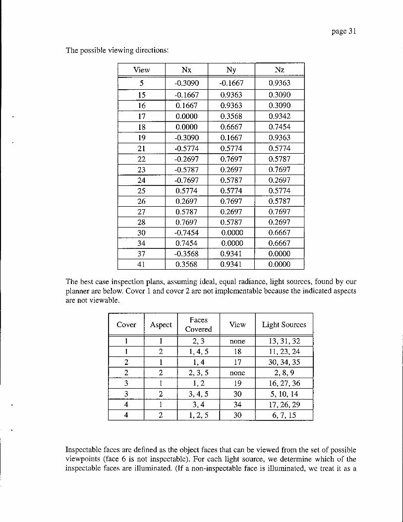
page 31
The possible viewing directions:
View Nx Ny Nz
5 -0.3090 -0.1667 0.9363
15 -0.1667 0.9363 0.3090
16 0.1667 0.9363 0.3090
17 0.0000 0.3568 0.9342
18 0.0000 0.6667 0.7454
19 -0.3090 0.1667 0.9363
21 -0.5774 0.5774 0.5774
22 -0.2697 0.7697 0.5787
23 -0.5787 0.2697 0.7697
24 -0.7697 0.5787 0.2697
25 0.5774 0.5774 0.5774
26 0.2697 0.7697 0.5787
27 0.5787 0.2697 0.7697
28 0.7697 0.5787 0.2697
30 -0.7454 0.0000 0.6667
34 0.7454 0.0000 0.6667
37 -0.3568 0.9341 0.0000
41 0.3568 0.9341 0.0000
The best case inspection plans, assuming ideal, equal radiance, light sources, found by our planner are below. Cover 1 and cover 2 are not implementable because the indicated aspects are not viewable.
Cover Aspect Faces
Covered View Light Sources
1 1 2,3 none 13,31,32
1 2 1,4,5 18 11,23,24
2 1 1,4 17 30, 34, 35
2 2 2,3,5 none 2,8,9
3 1 1,2 19 16, 27, 36
3 2 3,4,5 30 5, 10, 14
4 1 3,4 34 17, 26, 29
4 2 1,2,5 30 6,7,15
Inspectable faces are defined as the object faces that can be viewed from the set of possible viewpoints (face 6 is not inspectable). For each light source, we determine which of the inspectable faces are illuminated. (If a non-inspectable face is illuminated, we treat it as a

page 32
"don't care".) The different combinations of illuminated faces form illumination aspects. These aspects are formed into exact illumination covers. We used our "largest aspect" heu- ristic, with a search depth of one, to form the exact covers. It is possible that an illumination aspect contains a combination of object faces that is not viewable. This leads to the cases like covers 1 and 2, which both contain illumination aspects that are not viewable. (If a potential viewpoint views a non-inspectable face, we treat it as a "don't care".)
We implemented a near best case inspection plan for faces 3 and 4 using light sources 22, 29, 33 and viewpoint 34. The near worst case plan for faces 3 and 4 was light sources 22, 26, 29 and viewpoint 34. The planner determined that faces 1, 2, and 5 could only be illumi- nated by light sources 6,7,15. The camera viewpoint for faces 1, 2, and 5 was viewpoint 30.
We implemented these inspection plans on our experimental setup. The results, using mea- sured radiance light sources:
•-•£ • : •.•,•-£',:*>■■■■ ■•• •. • '•>•< . '•. '. f-.. •••>•!>; .'•* -WV. '.Ufa* >-•""•;• » -..-•\.«.,.i.. v. . .,* - .-\. Ht.^ •?:-.*••
• • ■fr'-'.'-.-r-r''' ' ■:'':■'•?'•■■ *•<;•'••':•'• ■*-■■:•-■■?•.
Planner Predictions
Measurements
Face Light
Sources Pixel
Number Degrees °(eerr)- Degrees
3 22,29,33 1 1.92 1.81 3 22,29,33 2 1.92 1.81 3 22,26,29 1 2.55 2.90 3 22,26,29 2 2.55 3.00 4 22,29,33 3 1.95 1.98 4 22,29,33 4 1.95 2.10 4 22,26,29 3 2.78 3.01 4 22,26,29 4 2.78 3.06 1 6,7,15 5 1.82 1.91 1 6,7,15 6 1.82 1.85 2 6,7,15 7 1.75 2.14 2 6,7,15 8 1.75 2.08 5 6,7,15 9 1.80 1.70 5 6,7,15 10 1.80 1.98 5 6,7,15 11 1.80 1.72
5 6,7,15 12 1.80 1.68
Measurements were made by taking 1000 images with each light source. A small number of pixels (4) were recorded from each image. This produced a data stream for that pixel. By combining data streams for 3 light sources, we calculated a mean surface orientation and the standard deviation of surface orientation error.
In general, the measured standard deviation of orientation error are within 20% of the plan- ner. Many are within 10%.

page 33
The difference between the near best case and near worst case plans should be noted. For Face 3, the near best case illumination plan results in a 5.76° predicted error, 3a(9err). In contrast, the near worst case illumination plan results in 7.65° predicted error. For Face 4, the near best case illumination plan results in a 5.85° predicted error. In contrast, the near worst case illumination plan results in 8.34° predicted error.
Images of Faces 3 and 4 using light sources 22, 29, and 33. (Face 5 is not illuminated.)
g. 19. Intensity Images: Faces 3 and 4
Needle map produced by the intensity images from light sources 22, 29, and 33.
Fig. 20. Needle Map: Faces 3 and 4 of cube

page 34
Images of Faces 1, 2, and 5 using light sources 6, 7 and 15.
Fig. 21. Intensity Images: Faces 6, 7, and 15 of cube
Needle map produced by the intensity images from light sources 6, 7, and 15.
ttttll^l
Fig. 22. Needle Map Faces: 6, 7, and 15 of cube
Illumination aspects from the 1, 1, 1 viewing direction (Numbers are light source numbers.

page 35
Light sources that are shaded the same belong to the same illumination aspect.):
Fig. 23JWummätiönäspects from the 1, 1, 1 viewing direction
Illumination aspects from the -1, 1, 1 viewing direction (Numbers are light source numbers. Light sources that are shaded the same belong to the same illumination aspect.):
Fig. 24. Illumination aspects from the -1, 1, 1 viewing direction
Illumination aspects from the 0, 0, 1 viewing direction (Numbers are light source numbers.

page 36
Light sources that are shaded the same belong to the same illumination aspect.):
Fig. 25. Illumination aspects from the 0, 0, 1 viewing direction

page 37
8. 2D Concave Lambertian Illumination Now we consider the illumination of simple 2D concavities, concavities composed of two surface edges that are fully visible to each other. The illumination of a concavity requires the determination of visibility regions for the potential light sources. For the simple concavities that we are considering in our work, we define the visibility region as the extension of the surface edges that form the concavity. For example, if the concavity has sides at 45° and 135°, the region that can see the concavity is the visibility region extending from 45° to 135°. Any viewpoint in the visibility region can see both faces of the concavity, so the exact cover problem is trivial. (We do not consider partial visibility of a concave edge.)
135° Visibility Region 450
Fig. 26. Concave Visibility Region
Once we have determined the light source visibility region, we need to determine the opti- mal location for light source placement within that region.
Nayar [31] showed that a shape from intensity method, such as photometric stereo, applied to a concavity would produce a "pseudo shape". The pseudo shape is shallower than the real concavity and the pseudo shape is invariant to light source placement. So, no matter where we place our light sources within the visibility region, the pseudo shape recovered using a method such as photometric stereo will produce the same shape.
So, if the pseudo shape is invariant to light source placement, what constitutes the light source placement problem. We define two possible concave light source placement prob- lems. The first problem is inspection of the pseudo shape. Deviations in the real shape will cause deviations in the pseudo shape. Therefore, we can detect deviations in the real shape by comparing the ideal pseudo shape with the measured pseudo shape. Different light source placements will give different amounts of uncertainty in the pseudo shape. We want to find the light source placement that yields the highest reliability. The second concave inspection problem involves using the pseudo shape to recover the real shape using Nayar's interactive shape recovery algorithm. Depending on the initial reliability of the pseudo shape, the final shape of the iterative algorithm may be closer to the actual shape. One would want to find the light source placement that produced the most accurate final shape. In this paper, we will discuss the first problem, inspection of the pseudo shape.
The goal of inspecting the pseudo shape is to find the light source positions that produce the minimum amount of uncertainty in the pseudo shape. The way to think about this problem is that interreflection, causes a distorted shape, the pseudo shape. The pseudo shape stays the same no matter where we place our light sources. So, the apparent object we are inspecting stays the same no matter where we place our light sources. This is equivalent to inspecting a

page 38
non-interreflecting lambertian object whose shape is equivalent to the pseudo shape. The process of interreflection that creates the pseudo shape is global, encompassing all of the surfaces that form the concavity. However, the problem of inspecting the pseudo shape is local. The reliability at each point of the pseudo shape only depends on the intensity at that point, not on any other points of the pseudo shape.
We can use the forward graphics solution [32] to predict the brightness of the concavity. The basic interreflection equation for diffuse surfaces is:
Radiosity = Emissions Interreflection
B{u) = E{u) +p(u) $F(u, v)B(v)dv D
F called the form factor. It is the fraction of the energy leaving surface u that arrives at sur- face v. E is the surface radiance due to a light source, p is the albedo of the surface. B is the aggregate surface radiance. D is all of the surfaces in the environment.
In discrete form, n
Bj = Ej + PjJjF(i,j)Bi j= hn
i= 1
where n is the number of elements in the environment.
For the two-dimensional case, with elements i and j. r is the distance between the centers of the elements. N; is the normal of element i. Nj is the normal of element j.
Fig. 27. Interreflection Geometry
The form factor [33] between elements i and j is:
COSÖ.COS0.
F{i,j) = V(i,j) 1 ids 2r
V is the visibility between face i and face j. V = 1 if face i can see face j. V = 0 otherwise. We use point to point form factors calculated between the center of each element, with a uni- form mesh and constant elements.
We can express the discrete form of the radiosity equation in matrix form
(I-PF)B = E

page 39
E and B are vectors of length n. E is the radiance of each element due to the light source. B is the aggregate radiance of an element due to interreflection and the light source.
F is the square matrix of form factors.
F =
FU F\2
F2\ ^22
In
n\
.. F. 33
... F„
P is the diagonal albedo matrix.
P =
pl 0 0 0
0 Pl 0 0
0 0 P3 0
0 0 0 Pn_
In the forward solution, we know P, F, and E. We want to solve for B, the brightness of the concavity with interreflection. The matrix equation is solved using the successive over relaxation method [34], with w = 1.4. Convergence usually occurs in approximately 15 iter- ations.
We solve the forward problem for two light sources, SI and S2. SI produces the brightness distribution Bl. S2 produces the brightness distribution B2. Once we have Bl and B2, we can solve for the pseudo shape using Bl, SI, B2, and S2.
-.-i Six Sly S2x S2y_
Bl[i]
B2[i]
Nx[i]
Ny[i] .,n
Where Nx and Ny are the normals of the pseudo shape, and n is the number of face ele- ments.
If our goal is to inspect the pseudo shape with the most reliability possible, then the analysis from here on is very similar to the 2D and 3D convex cases. The difference between the con- vex case and the pseudo shape case is that the pseudo shape is non-planar. The uncertainty for a planar convex face is constant since the variance of the face depends on the face's nor- mal direction and the light source direction. A pseudo shape face is curved. Therefore, the uncertainty along the pseudo shape face varies. We could minimize the average angular ori- entation error of a pseudo shape face, or if we were interested in a particular point, we could minimize the angular orientation error of that point. For the experiments that follow, we seek to minimize the error at the center of each face.
If B1 and B2 are the nominal light source intensities, noise in either B1 or B2 will cause an

page 40
error in Nx and Ny, producing a noisy normal:
-i Six Sly S2x S2y_
Bl[i] + 651 [i]
B2[i] +852[/] Nx[i] +8Nx[i]
Ny[i] +8Ny[i] i = i, ..., n
If we were to measure B1 and B2, both of which might be corrupted by errors, and we were to solve for Nx and Ny, we would normalize the resulting values of Nx and Ny because the surface normal is by definition a unit vector. The noisy, normalized, normal is:
N[i], Nx[i]+ 8Nx [i] Ny [i] + SNy [i]
\N[i] +8N[i]\ ' \N[i] +8N[i]\
N[i] . = Nx[i] . ,Ny[i] . ' noise L J niose J L J noise
i, ..., n
We define the orientation error to be the angle between the nominal unit normal and the noisy unit normal. We have the planner conduct a simulation using the intensity noise func- tion. If we know, the nominal intensity of each light source (This can be determined if the object's pose is known, if the light source directions are known, and if the light source's albedos are known.) and the corresponding value of a;, we can calculate a noisy surface ori- entation using the known light source positions. At each iteration, a random intensity for each light source is determined based on the mean light source intensity and a; for that light source intensity. These three noisy intensity values are used to determine a noisy surface ori- entation. We repeat this 1000 times. We calculate the mean, noisy, surface orientation to be the center of mass of the 1000 noisy surface orientations:
1000 1000
N[i],
y [Nx[i] . ] y [Ny[i] . ] i-i L L J noise1 j £-t L J L J noise* j i = i, ..., n
_ .7=1 y=i 1000 1000
Using each noisy surface orientation and the mean, noisy, surface orientation, we calculate the orientation error.
Q[i] = acos (W [i] „,„■•#[*] . ) / - ,■ „ L J err v L J noise L 'noise' ' — '> ...,«
Using the 1000 values of orientation error that our simulation produced, we then determine the standard deviation of surface orientation error, cr(0err).
We have performed simulations on a range of simple 2D concavities to explore the relation- ship between tf(0err) and concavity shape.

page 41
The first concavity we looked at had a concavity of 140°. p= 0.8. n = 500. The intensity of both light sources was 200. Both sides of the concavity are the same length.
20° Face "A"
S Face "B'
20° N.
Fig. 28. 140° 2D Concavity
The shape and pseudo shape are shown here (The pseudo shape is the more concave shape.):
Fig. 29. 140° 2D Concavity Shape and Pseudo Shape
The error surface of 6errface for Face "A" is (SI, S2, and error are all in degrees):
3a(0eiT) for center of Face A
3a(9err) for center of Face A
150
150
lOO^^^^^^^lOO s2 150.50 sl
3a(6err) for center of Face A
100 150 50 s2
Fig. 30. 140° 2D Concavity Error Surface for center of Face A
The maximum error is 37.5°. The minium error is 1.5°. The search was conducted in 5° increments.

page 42
The second concavity we looked at had a concavity of 90°. p= 0.8. n = 500. The intensity of both light sources was 200. Both sides of the concavity are the same length.
45° \ Face "A" Face "B>x 45o ce'A" Face"B'>
Fig. 31. 90° 2D Concavity
The shape and pseudo shape are shown here (The pseudo shape is the more concave shape.):
Fig. 32. 90° 2D Concavity Shape and Pseudo Shape
The error surface of 0err_face for Face "A" is (SI, S2, and error are all in degrees): 3c(0erT) for center of Face A
3a(0err) for center of Face A
3a(0err) for center of Face A
10 S2 12
00 20 SI
3G(0err) for center of Face A
SI 150 50 s2
Fig. 33. 90° 2D Concavity Error Surface for center of Face A
The maximum error is 35.6°. The minium error is 2.0°. The search was conducted in 5° increments.

page 43
The third concavity we looked at had a concavity of 45°. p= 0.8. n = 500. The intensity of both light sources was 200. Both sides of the concavity are the same length.
67.5C / 67.5C
Face "A Face "B'
Fig. 34. 45° 2D Concavity
The shape and pseudo shape are shown here (The pseudo shape is the more concave shape.):
Fig. 35. 45° 2D Concavity Shape and Pseudo Shape
The error surface of 9erT face for Face "A" is (SI, S2, and error are all in degrees):
3o(9err) for Face center of A 3G(6err) for center of Face A
3a(0err) for center of Face A
3a(0err) for center of Face A
A I V 50"
15( .50 150 50
100 SI XJU "" S2
Fig. 36. 45° 2D Concavity Error Surface for center of Face A
40
30
20
10
0 ■^50
00 SI
The maximum error is 36.8°. The minium error is 6.7°. The search was conducted in 5° increments.

page 44
As the concavity becomes more acute, the pseudo shape becomes deeper and more concave. In addition, as the concavity becomes more acute, the visibility region becomes more acute. These two factors combine to increase the minimum error for a face. (The maximum error is largely a function of the separation between the light sources.)
As shown in section 3.4.1., a lambertian shape will produce high reliability when the angle between the light sources and normal are large. As a concavity becomes more acute, and the pseudo shape becomes deeper and more concave, the maximum angle between viewpoints in the visibility region and points along the pseudo shape will be smaller. This will cause the error to be larger, and more of the visibility region will produce large errors. For a shallow concavity, the pseudo shape will be less concave. Less of the visibility region will be at acute angles to the pseudo shape. The maximum angle between viewpoints in the visibility region and points along the pseudo shape will be larger. This will cause the error to be smaller, and less of the visibility region will produce large errors.
We also looked at the variation of error along each face of the pseudo shape. (Points 0 to 249 belong to pseudo shape face A. Points 250 to 499 belong to pseudo shape face B. si = 72.5°, s2 = 107.5°, rho = 0.8)
6.0
t CD
CO
100.0 200.0 300.0 400.0 500.0 Point Number Fig. 37. Error across face A and Face B forl40° concavity
b CD
to"
0.0 100.0 200.0 300.0 400.0 500.0 Point Number
Fig. 38. Error across face A and Face B for 90° concavity

page 45
h tu
CD
b' CO
0.0 100.0 200.0 300.0 400.0 500.0 Point Number
Fig. 39. Error across face A and Face B for 45° concavity
The variation in error along a face is a function of the curvature of the pseudo shape face. If the pseudo shape face is approximately flat, the angle between the light sources and face are approximately constant. Therefore, the error along the face is approximately constant. If the pseudo shape face has a high curvature, the angle between the light sources and face will vary. This will cause the error along the face to vary. The 45° concavity's pseudo shape has the highest curvature. Therefore, the error along its face varies the most.

page 46
9. 3D Concave Lambertian Illumination Now we consider the illumination of simple 3D concavities, concavities composed of two rectangular faces that are fully visible to each other. The solution of the 3D concave illumi- nation problem is very similar to the solution of the 2D concave illumination problem.
For the three-dimensional case, with elements i and j. r is the distance between the centers of the elements. N; is the normal of element i. Nj is the normal of element j.
Ni
Fig. 40. Interreflection Geometry
The form factor [35] between elements i and j is:
F(i,j) = V(i,j) cos0.cos9.
' J dA:
nr
V is the visibility between face i and face j. V = 1 if face i can see face j. V = 0 otherwise. dAj is the differential area of facet j.
We solve the forward problem for three light sources, SI, S2, and S3. SI produces the brightness distribution Bl. S2 produces the brightness distribution B2. S3 produces the brightness distribution B3. Once we have B1, B2, and B3, we can solve for the pseudo shape using Bl, SI, B2, S2, B3, and S3.
Six Sly Slz Six Sly Slz _S3x S3y S3z
Bl Nx Bl = Ny B3 Nz
Our goal is to inspect the pseudo shape with the highest reliability possible. The analysis from here on is identical to the 3D convex case, Section 5.1.. We would use Bl, B2, B3, Nx, Ny, and Nz to calculate the angular orientation error at each point on the pseudo shape. The difference between the convex case and the pseudo shape case is that the pseudo shape is non-planar. The uncertainty for a planar convex face is constant since the variance of the face depends on the face's normal direction and the light source direction. A pseudo shape face is curved. Therefore, the uncertainty along the pseudo shape face varies. We could min- imize the average angular orientation error of a pseudo shape face, or if we were interested in a particular point, we could minimize the angular orientation error of that point. For the experiments that follow, we seek to minimize the error at the center of each face.

page 47
9.1. Implementation
We implemented our 3D concave planner in C instead of in LISP because of the large com- putational expense involved in the forward prediction problem. Our 3D planner accepts the vertex coordinates of two rectangular faces. Each face is tessellated into an NxN grid of ele- ments. (For these experiments N = 15.) All combinations of light sources that are visible to both faces are included in a potential source list. The forward prediction is performed for each combination of light sources in the source list. Then, the angular orientation error is calculated at the center of both faces. A viewpoint that satisfies the minimum foreshortening criteria is used.

page 48
10. 3D Concave Lambertian Illumination Experiments Experiments were conducted to validate the concave lambertian illumination planner. We wanted to verify that the illumination plans generated by the planner were valid and accu- rate. In order to do this, we tested the results of the planner for a set of illumination plans. One set of plans tested was near the most accurate illumination plan generated by our illumi- nation planner. The other set of plans tested was near the least accurate illumination plan generated by our illumination planner. The results of the two plans were compared with each other and with the planner's predictions. We also verified that the light source view- point visibility and camera viewpoint visibility predicted by the planner were correct.
10.1. Chalk Concavity
We constructed a simple concavity. Two rectangular faces were milled out of railroad chalk. The two faces were held in a holder that formed a 90° concavity.
The concavity was oriented so that the X, Y, and Z axes intersect at the center of the concav- ity. The X axis coincides with the cusp of the concavity. The Z axis bisects the concavity (it points up). By using a Macbeth ColorChecker color rendition chart, we determined that the albedo of the railroad chalk was 0.936.
Face A FaceB
Holder
Fig. 41. 90° Chalk Concavity
The nominal orientation of the concavity's faces is shown in the table below.
Face Nx Ny Nz
A 0.0 0.707 0.707
B 0.0 -0.707 0.707
Our light sources are 2" in diameter and they are 9" from our object. They subtend an angle of 12.5°. In order to ensure that all of the light source is visible to each illuminated face, we impose a limit on the light source incident angle. The angle between a light source and Face A or Face B cannot be more than 77.5°. Seven light sources satisfy this condition: SI, S2, S3, S5, S6, Sll, and S12. We measured the intensities of these light sources using the same material that the chalk faces were made of.

page 49
The possible light source directions:
Light Source
Nx Ny Nz Source Intensity
1 -0.3090 -0.5000 0.8090 176.2
2 0.3090 -0.5000 0.8090 207.0
3 0.0000 0.0000 1.0000 207.4
5 0.5257 0.0000 0.8507 185.7
6 -0.5257 0.0000 0.8507 205.2
11 0.3090 0.5000 0.8090 192.3
12 -0.3090 0.5000 0.8090 208.2
The possible viewing directions:
View Nx Ny Nz
5 -0.3090 -0.1667 0.9363
15 -0.1667 0.9363 0.3090
16 0.1667 0.9363 0.3090
17 0.0000 0.3568 0.9342
18 0.0000 0.6667 0.7454
19 -0.3090 0.1667 0.9363
21 -0.5774 0.5774 0.5774
22 -0.2697 0.7697 0.5787
23 -0.5787 0.2697 0.7697
24 -0.7697 0.5787 0.2697
25 0.5774 0.5774 0.5774
26 0.2697 0.7697 0.5787
27 0.5787 0.2697 0.7697
28 0.7697 0.5787 0.2697
30 -0.7454 0.0000 0.6667
34 0.7454 0.0000 0.6667
37 -0.3568 0.9341 0.0000
41 0.3568 0.9341 0.0000
The planner selected viewpoint 5 as the least foreshortening viewpoint.
We implemented two near best case inspection plans and two near worst case inspection plans. The planner predictions and measurements are for a point near the center of each Face.
In general, the predictions for the best case inspections plans are within 15% of the predic- tions. The predictions for the worst case inspections plans are not as accurate with errors

page 50
running up to 30%. The reason for the difference in accuracy is the very nature of the best case versus worst case plans. The best case inspection plans produce a small amount of error when there is a disturbance in intensity. We have been considering this disturbance to be from the light intensity variance of the CCD and digitizer. The best case plan has a low sen- sitivity to this noise, while the best case plan has a high sensitivity. Our chalk surface is not perfectly lambertian. So, there discrepancies between the intensities that our planner pre- dicts and our measurements. Since our worst case plan has a higher sensitivity to these intensity deviations, the accuracy of these plans is worse. This observation makes us con- clude that less sensitive plans will also produce more accurate results when there are devia- tions from the expected photometric model.
^^^^^^^^^^^^^B Planner
Predictions Measurements
Face (center of face)
Light Sources Degrees
aOerr) " Degrees
A 1,12,6 4.05 4.71 B 1,12,6 4.11 4.97 A 1,12,5 1.23 1.42 B 1,12,5 1.22 1.35 A 2,11,6 1.14 1.25 B 2,11,6 1.15 1.26 A 2,11,5 4.22 3.05 B 2,11,5 4.23 3.51
The deviation that we measured between the chalk and the ideal lambertian model is shown below.
1.00
«3 G 0.80 (l) 4-*
G
T) 0.60 fli N
s 5-1
0.40
o £ 0.20
0.00 0.0 20.0 40.0 60.0 80.0
Viewing Angle Fig. 42. Chalk: Intensity Versus Viewing Angle. (Incident Angle = 0° )
A lambertian surface's intensity should be viewer independent. The chalk exhibits some

page 51
reduction in intensity with increased viewing angle. This caused the brightness predicted by the planner to be greater than measurements. The next table lists predicted brightness versus measured brightness near the center of each face.
Planner Prediction
Measurement Percent Error
Face (center of face)
Sources in Group
Light Source
I I
A 1, 12,6 1 61.0 57.4 -5.9 A 1, 12,6 12 165.3 150.0 -9.3 A 1,12,6 6 119.0 113.1 -5.0 B 1,12,6 1 165.3 147.3 -10.9 B 1,12,6 12 61.0 52.7 -13.6 B 1,12,6 6 119.0 109.8 -7.7 A 1,12,5 1 61.0 57.4 -5.9 A 1,12,5 12 165.3 150.0 -9.3 A 1,12,5 5 119.0 99.2 -16.6 B 1,12,5 1 165.3 147.3 -10.9 B 1,12,5 12 61.0 52.7 -13.6 B 1,12,5 5 119.0 97.0 -18.5 A 2, 11,6 2 66.8 64.4 -3.6 A 2,11,6 11 181.1 171.0 -5.6 A 2,11,6 6 130.3 124.0 -4.8 B 2,11,6 2 181.1 164.4 -9.4 B 2,11,6 11 66.8 55.3 -17.2 B 2,11,6 6 130.3 120.2 -7.8 A 2,11,5 2 64.4 62.1 -3.6 A 2,11,5 11 174.6 164.8 -5.6 A 2,11,5 5 125.7 104.8 -16.6 B 2,11,5 2 174.6 158.5 -9.2 B 2,11,5 11 64.4 53.3 -17.2 B 2,11,5 5 125.7 102.4 -18.5
We measured a 10X10 array of points on each face of the concavity. This allows us to com- pare the predicted and measured error surfaces, 3a(0err), Fig. 39 and Fig. 41.
We are also able to compare the predicted and measured intensity profiles for each face. The shape of the two surfaces is very close. As expected, the measured intensity surface is atten- uated, Fig. 40 and Fig. 42.
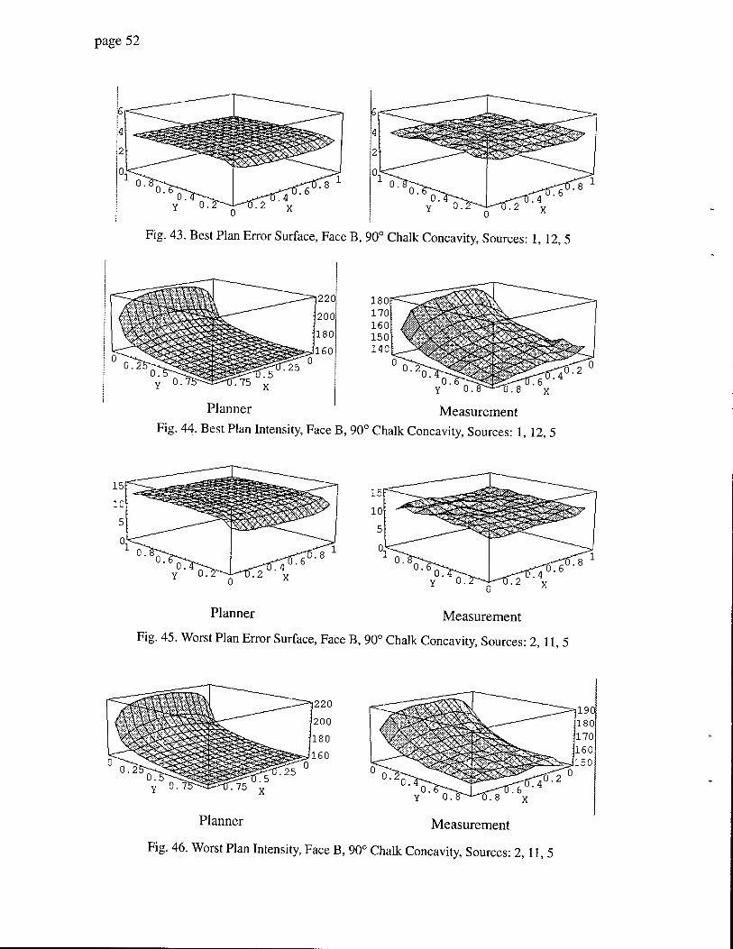
page 52
Fig. 43. Best Plan Error Surface, Face B, 90° Chalk Concavity, Sources: 1, 12, 5
Planner Measurement Fig. 44. Best Plan Intensity, Face B, 90° Chalk Concavity, Sources: 1, 12, 5
Planner Measurement
Fig. 45. Worst Plan Error Surface, Face B, 90° Chalk Concavity, Sources: 2, 11, 5
Planner Measurement
Fig. 46. Worst Plan Intensity, Face B, 90° Chalk Concavity, Sources: 2,11, 5

page 53
An intensity image of the concavity and a needle map of the concavity is shown in Fig. 43..
Fig. 47. Intensity Image from Source 1, and needle map from sources: 1, 12, 5

page 54
11. Conclusions We have developed an illumination planner for convex lambertian objects and for simple lambertian concavities. The planner determines how to position light sources around an object so that we illuminate a specified set of faces in an efficient manner. Using a noise model of the CCD, a CAD model of the object we are inspecting, and the lambertian reflec- tance model, the planner performs a statistical simulation to determine how much uncer- tainty we can expect in our shape measurement for a given light source configuration. The planner generates an illumination plan that illuminates the specified set of object faces while having a minimum amount of uncertainty. We have verified that the illumination plans gen- erated by the planner are valid and accurate.
This work has potential applications to inspection problems in industrial environments. Although the photometric stereo method requires careful calibration. We have shown that it is possible to accurately predict measured shape uncertainty. This ability can be used to reli- ably detect defects.

page 55
12. References [I] C. Cowan, "Automatic Sensor Placement from Vision Task Requirements", IEEE
Trans, on Pattern Analysis and Machine Intelligence, Vol. 10, No. 3, pp. 407-416, May, 1988.
[2] C. Cowan, "Determining the Camera and Light Source Location for a Visual Task", 1989 IEEE International Conference on Robotics and Automation, pp. 509-514.
[3] C. Cowan, "Automatic Camera and Light Source Placement Using CAD Models", IEEE Workshop on Directions in Automated CAD-Based Vision", June 1991, Maui, Hawaii, pp. 22-31.
[4] R. Tsai and K. Tarabanis, "Occlusion Free Sensor Placement", Yorktown Heights, NY: TJ. Watson Research Center, RC 14593, March 1989.
[5] R. Tsai and K. Tarabanis, "Satisfying the Resolution Constraint in the "MVP" Machine Vision Planning System", Proceedings DARPA Image Understanding Workshop, Pittsburgh, P.A., September 11-13, 1990.
[6] R. Tsai, K. Tarabanis, and P. Allen, "Automated Sensor planning for robotic vision tasks", 1991 IEEE International Conference on Robotics and Automation, pp. 76-82.
[7] G. Hager, "Active Reduction of Uncertainty in Multi-sensor systems", University of Pennsylvania, Philadelphia, Pennsylvania, Ph.D. Thesis, MS-CIS-88-47.
[8] G. Hager, "Computational Methods For Task-Directed Sensor Data Fusion and Sen- sor Planning", University of Pennsylvania, Philadelphia, Pennsylvania, MS-CIS-90- 38.
[9] S. Sakane, M. Ishii, and M. Kakikura, "Occlusion avoidance of visual sensors based on a hand-eye action simulator system: HEAVEN", Advanced Robotics, Vol. 2, No 2, pp. 149-165.
[10] S. Sakane, T. Sato, and M. Kakikura, "Automatic Planning of Light Source Place- ment for an Active Photometric Stereo System", 1990 IEEE International Workshop on Intelligent Robots and Systems, pp. 559-556.
[II] S. Sakane and T. Sato, "Automatic Planning of Light Source Placement and Camera Placement for an Active Photometric Stereo System", 1991 IEEE International Con- ference on Robotics and Automation, pp. 1080 - 1087.
[12] R. Niepold, S. Sakane, T. Sato, and Y. Shiraii, "Vision Sensor Set-up for a Hand-Eye System Using Environmental Model", SICE 87, pp. 1037-1040.
[13] S. Yi, R. Haralick, and L. Shapiro, "Automatic Sensor and Light Source Placement for Machine Vision", University of Washington, Seattle, Washington, CS-89-11-03.

page 56
[14] S. K. Nayar, K. Ikeuchi, T. Kanade, "Surface Reflections: Physical and Geometrical Perspectives", IEEE Trans, of Pattern Analysis and Machine Intelligence, Vol. 13, No. 7, pp. 611-634, July, 1991.
[15] J. J. Koenderink and A. J. van Doom, "The Internal Representation of Solid Shape with Respect to Vision", Biol. Cybernetics, Vol. 32, pp. 211-216, 1979.
[16] K. Ikeuchi and T. Kanade, "Automatic Generation of Object Recognition Pro- grams", Proceedings of the IEEE, Vol. 76, No. 8, pp. 1016-1035, August, 1988.
[17] M. Hebert and T. Kanade, "The 3D-Profile Method of Object Recognition", 1985 IEEE Conference on Computer Vision and Pattern Recognition, pp. 458-463.
[18] Z. Gigus, J. Canny, and R. Seidel, "Efficiently Computing and Representing Aspect Graphs of Polyhedral Objects", IEEE Trans, of Pattern Analysis and Machine Intel- ligence, Vol. 13, No. 6, pp. 542-551, June, 1991.
[19] D. Kriegman and J. Ponce, "Computing Exact Aspect Graphs of Curved Objects: Solids of Revolution", International Journal of Computer Vision, Vol. 5, No. 2, pp 119-135.
[20] J. Stewman and K. Bowyer, "Aspect Graphs for Convex Planar-Face Objects", IEEE Workshop on Computer Vision", Miami, Florida, 1987.
[21] H. Plantinga and C. Dyer, "Visibility, Occlusion, and the Aspect Graph", Interna- tionaljournal of Computer Vision, Vol. 5, No. 2, pp. 137-160.
[22] K. Bowyer and C. Dyer, "Aspect Graphs: An Introduction and Survey of Recent Results", International Journal of Imaging Systems and Technology, Vol 2, No 4 1990, pp. 315-328.
[23] B. G. Batchelor, D. A. Hill, and D. C. Hodgson, "Automated Visual Inspection", 1985, IFS (Publications) Ltd., Bedford, U.K.
[24] B. G. Batchelor, "A Prolog Lighting Advisor", Intelligent Robots and Computer Vision VIII: Systems and Applications, Bruce G. Batchelor, Editor, Proc. SPIE 1193.
[25] B. G. Batchelor and F. M. Waltz, Editors, "Machine Vision Systems Integration", 1990, SPIE Optical Engineering Press, Bellingham, Washington.
[26] G. Healey and R. Kondepudy, "CCD Camera Calibration and Noise Estimation", 1992 IEEE International Conference on Computer Vision and Pattern Recognition pp. 90 - 95.
[27] G. Healey and R. Kondepudy, "Modeling and Calibrating CCD Cameras for Illumi- nation Insensitive Machine Vision", Optics, Illumination, and Image Sensing for Machine Vision VI, Proc. SPIE 1614.

page 57
[28] R. Ray, J. Birk, and R. Kelley, "Error Analysis of Surface Normals Determined by Radiometry", IEEE Trans, of Pattern Analysis and Machine Intelligence, Vol. 5, No. 6, pp. 631-645, November, 1983.
[29] W. Press, B. Flannery, S. Teukolsky, W. Vetterling, "Numerical Recipes in C", Cam- bridge University Press, New York, 1990, pp. 490 - 494.
[30] B. Kumar, J.C. Robert, R. Hoffman, K. Ikeuchi. and T. Kanade, "Vantage, A Frame Based Geometric Modeling System Programmer/Users Manual V2.0", CMU-RI- TR-91-31, December 1991.
[31] S. K. Nayar, K. Ikeuchi, T. Kanade, "Shape from Interreflections", Proceedings of the Third International Conference on Computer Vision, pp. 2-11, December 1990.
[32] C. Goral, K. Torrance, D. Greenberg, and B. Battaile, "Modeling the Interaction of Light Between Diffuse Surfaces", Proceedings ofSIGGRAPH84, Vol. 18, No. 3, pp. 213- 221, July, 1984.
[33] P. Heckbert, "Simulating Global Illumination Using Adaptive Meshing", Ph.D. The- sis, University of California, Berkeley, UCB/CSD 91/636, June, 1991.
[34] G. Golub and C. Van Loan, "Matrix Computations", The Johns Hopkins University Press, Baltimore, 1989, pp. 510-511.
[35] E. M. Sparrow and R. D. Cess, "Radiation Heat Transfer", McGraw-Hill, New York, 1978.
[36] B. M. Oliver, "Thermal and Quantum Noise", Proceeding of IEEE, Vol 53, pp. 436- 454, May 1965.
[37] S. K. Nayar and H. Murase, "Illumination Planning for Object Recognition in Struc- tured Environments", 1994 IEEE International Conference on Computer Vision and Pattern Recognition, pp. 31-38.
[38] G. Strang, "Linear Algebra and Its Applications", Harcourt Brace Jovanovich, New York, 1988.