tanagra rule induction -...

Tutorial – Case studies R.R.

15 février 2010 sur 31

1. Topic

Supervised rule induction – Software comparison.

Supervised rule induction methods play an important role in the Data Mining context. Indeed, it provides an easy to understand classifier. A rule uses the following representation: “IFIFIFIF premise THENTHENTHENTHEN conclusion” (e.g. IF an account problem is reported on a client THEN the credit is not accepted).

Among the rule induction methods, the "separate and conquer" approaches are very popular during

the 90's. Curiously, they are less present today into proceedings or journals. More troublesome still, they are not implemented in commercial software. They are only available in free tools from the Machine Learning community. However, they have several advantages compared to other techniques.

Compared to classification tree algorithms (http://en.wikipedia.org/wiki/Decision_tree_learning) which are based on the divide and conquer paradigm, their representation bias is more powerful because it

is not constrained by the arborescent structure. It needs sometimes a very complicated tree to get an equivalent of a simple rule based system. Some splitting sequences are replicated into the tree. It is known as the "replication problem". The other consequence is that the induction bias is not the same. The tree searches the average purity on the leaves when it splits a node. The separate and conquer on the other hand tries to maximizes the purity of one leaf only when it tries to create a rule.

Compared to the predictive association rule algorithms (e.g. http://www.comp.nus.edu.sg/~dm2/), they

do not suffer of the redundancy of the induced rules. The idea is even to produce the minimal set of rules which allows to classify accurately a new instance. It enables to handle the problem of collision about rules, when an instance activates two or several rules which lead to inconsistent conclusions.

In this tutorial, we describe first two separate and conquer algorithms for the rule induction process. Then, we show the behavior of the classification rules algorithms implemented in various tools such as

Tanagra 1.4.34Tanagra 1.4.34Tanagra 1.4.34Tanagra 1.4.34, Sipina Sipina Sipina Sipina ReReReResearchsearchsearchsearch 3.33.33.33.3, Weka 3.6.0Weka 3.6.0Weka 3.6.0Weka 3.6.0, R 2.9.2R 2.9.2R 2.9.2R 2.9.2 with the RWeka package, RapidMiner 4.6RapidMiner 4.6RapidMiner 4.6RapidMiner 4.6, or Orange 2.0bOrange 2.0bOrange 2.0bOrange 2.0b.

2. The« separate-and-conquer » paradigm

The goal is to learn a prediction rule from data

IfIfIfIf Premise ThenThenThenThen Conclusion

« Premise » is a set of conditions « attribute – Relational Operator – Value ». For instance,

Age > 45 andandandand Profession = Workman

In the supervised learning framework, the attribute into the conclusion part is of course the target attribute. A rule is related to only one value of the target attribute. But one value of the target attribute may be concerned by several rules.



Basically, the separate and conquer algorithms are based on the sequential covering principle1: we

define a rule which accurately predict one value of the target attribute (conquer); we remove the covered examples from the learning set (separate); we iterate the process until all the training instances are covered. They belong to the AQ family algorithms (Michalski, 1969).

Based on this framework, two approaches are usually implemented. The bottom-up approach starts from a positive instance; it tries to generalize the rule by removing some conditions. The rule must

cover the largest set of positive instances with the fewest negative instances. This method is often quite slow, especially on large and noisy dataset. On the contrary, the top-down approach is similar to the classification tree induction. But we try to maximize only the purity of the leaf on a branch of the tree. The calculation time is very similar to the induction tree algorithms.

In this tutorial, we present two methods based on the top-down separate-and-conquer principle. They correspond to two variants of the famous CN2 induction rule algorithm2 implemented into Tanagra.

They can handle directly multiclass problems (the target attribute can take more than 2 values).

2.1. Induction of ordered rules - Decision list induction

The first CN2 algorithm (Clark and Niblet, 1989) allows to induce a decision list (Rivest, 1987). It is an ordered and mutually exclusive set of rules. When we want to classify a new instance, the first rule is

evaluated. If it is not fired, we test the second rule, and so on, until a rule is fired. If no rule is activated, we use the default rule.

The rule based system has the following structure:

IFIFIFIF Condition 1 ThenThenThenThen Conclusion 1 Else IfElse IfElse IfElse If Condition 2 ThenThenThenThen Conclusion 2

Else IfElse IfElse IfElse If… Else IfElse IfElse IfElse If (Default rule) Conclusion M

The main advantage of this representation is that we cannot have rule conflict. One and only one rule is activated when we want to classify a new instance.

N° Antecedent Consequent Distribution

1 IF physician-fee-freeze in [y] -- synfuels-corporation-cutb in [n] Class in [republican] (135; 3)

2 ELSE IF physician-fee-freeze in [n] Class in [democrat] (2; 245)

3 ELSE (DEFAULT RULE) Class in [republican] (31; 19)

Figure Figure Figure Figure 1111 –––– Decision list on Vote datasetDecision list on Vote datasetDecision list on Vote datasetDecision list on Vote dataset

We obtain a set of 3 rules on the Congress Vote dataset3 (Figure 1). The aim is to detect the political group membership of congressmen from the votes on various topics.

1 J. Furnkranz, « Separate-and-Conquer Rule Learning », Artificial Intelligence Review, Volume 13, Issue 1, pages

3-54, 1999. 2 P. Clark and T. Niblett, « The CN2 Induction Algorithm », Machine Learning, 3(4) :361 :283, 1989.

P. Clark and R. Boswell, « Rule Induction with CN2 : Some recent improvements », Machine Learning – EWSL-

91, pages 151-163, Springer Verlag, 1991.

See also : http://www.cs.utexas.edu/users/pclark/software/



The “antecedent” is the premise of the rule; the “consequent” is the conclusion. The distribution

displays the occurrence of each values of the target attribute among the covered instances.

When we want to classify an instance with the following characteristics (Physician-fee-freeze = y; Synfuels-corporation-cutb = y), we observe that only the default rule is activated. Thus we assign to the instance the "republican" label.

We observe that we can obtain the same set of rules with the induction graphs algorithm4 (Figure 2).

This last one is a generalization of the classification tree approach where we can merge nodes. But the rule based classifier is definitely more compact (and easier to understand) whereas the two classifiers are logically identical.

Figure Figure Figure Figure 2222 –––– Decision graph on the “ Decision graph on the “ Decision graph on the “ Decision graph on the “Vote” datasetVote” datasetVote” datasetVote” dataset

Decision list induction algorithmDecision list induction algorithmDecision list induction algorithmDecision list induction algorithm

The induction process is based on the top down separate and conquer approach. We have two nested procedures. The first is intended to create the set of rules from the target attribute, the input variables

and the instances.

3 http://archive.ics.uci.edu/ml/datasets/Congressional+Voting+Records

4 D. Zighed, R. Rakotomalala, « Graphes d’Induction : Apprentissage et Data Mining », Hermès, 2000.

See also R. Rakotomalala, « Graphes d’Induction », PhD Dissertation, University Lyon 1, 1997 ; chapter 7.



Decision List (target, inputs, instances)

Ruleset = ∅

Repeat

Rule = Specialize (target, inputs, instances)

If (Rule != NULL) Then

Ruleset = Ruleset + {Rule}

Instances = Instances – {Instances covered by the rule}

End if

Until (Rule = NULL)

Ruleset = Ruleset + {Default rule (instances)}

Return (Ruleset)

At each step, the algorithm creates the best rule by a top down search using the available instances. The process is continued until one cannot create a new rule. The default rule is based simply on the remaining instances; the conclusion corresponds to the most frequent value of the target attribute.

The “specialize” function is very important in the process. It is based on a top down search paradigm i.e. it sequentially adds the best, according to a certain purity measure, condition to the existing premise. The inability to improve the measure is the stopping rule. It is a hill climbing optimization5.

Specialize (target, inputs, instances) Rule = NULL Max.Measure = - ∞ While (Stopping.Rule(Rule) == FALSE) Ref.Measure = - ∞ For Each Candidate Proposition Measure = Evaluation (Rule, Proposition) If (Measure > Ref.Measure) Then Ref.Measure = Measure Proposition* = Proposition End If End For If (Ref.Measure > Max.Measure) Rule = Rule x Proposition* Max.Measure = Ref.Measure End If End While Return (Rule)

The “evaluation” function plays two important roles during the specialization process:

1. It checks if the additional proposition enables to improve significantly the rule. On the one hand, it uses a chi-square test of independence (http://en.wikipedia.org/wiki/Pearson%27s_chi-

square_test#Test_of_independence). If the computed p-value is lower than the significance level of the test (« Signif.Level for pruning », the default value is 0.10), the additional proposition (condition) is accepted. On the other hand, it checks if the number of covered instances is upper

5 In the original CN2 algorithm (Clark and Niblett, 1989), the authors use a more sophisticated beam search

during the optimization process. This solution is implemented into the Orange software for instance. The

parameter "k" allows to specify the beam width. If we set k=1, we obtain a hill climbing optimization.



or equal than a predefined threshold. It is a support criterion (« Min. Support of Rule »6; the default

value is 10).

Here, we analyze the addition of the condition to the first rule of our first rule on the "Vote" dataset (Figure 1). We use the distribution outlined into the decision graph (Figure 2).

Root PHYSICIAN = Y SYNFUELS = NRepublican 168 ==> 163 ??? ==> ??? 135Democrat 267 14 3

With the additional condition, the rule covers 1383135 =+=an instances. It is larger than the

support threshold. About the chi-square test, we set the following cross tabulation.

+Synfuels = n Uncovered PhysicianRepublican 135 28 163Democrat 3 11 14Total 138 39 177

We obtain 29.282 =χ , the p-level is 71005.1 −× (< 0.10). The additional condition is validated.

2. The "evaluation" function is also used to measure the relevance of the rule. Two measures are available : the Shannon entropy, it highlighted the purity of the instances covered by the rule

(http://en.wikipedia.org/wiki/Entropy_%28information_theory%29); and the J-measure, it is rule-preference measure which quantifies the information content of a rule or a hypothesis (http://id3490.securedata.net/rod/pdf/RG.Paper.CP22.pdf). Beyond formulas and interpretations, we note mainly that the first leads to more specialized rules, and therefore more complex rule set. It is the best when we work on small non-noisy dataset. The second, however, favors simpler solutions, leads to fewer rules; each rule has a higher support. We use this last one when we deal

with large and noisy dataset.

Let kp the probability P(Y=k) the class distribution on the whole dataset, the initial class distribution;

akp / is the probability P(Y=k/a) for a rule with the condition « a », the conditional class distribution;

ap is the relative support of the rule, the “weight” of the rule.

We take the first rule RRRR of our classifier (Figure 1), we have the following values:

Root SYNFUELS = N

Republican 168 135

Democrat 267 3

Republican 0.386 0.978

Democrat 0.614 0.022

The Shannon entropy does not consider the initial class distribution.

6 In the supervised learning framework, the support of the rule corresponds to the number of instances

covered by the rule, whatever their target attribute value. The definition of the same term “support” is

different in the association rule mining context.



∑=k

akak ppaS // log)(

For RRRR, S(a) is

( ) ( )[ ] 151.0120.0022.0031.0978.0)( −=−×+−×=aS

The J-Measure considers the initial class distribution. We prefer also this measure when we deal with imbalanced dataset.

∑×=k k

ak

k

aka p

p

p

ppaJ // log)(

On the same rule RRRR, we have

( ) ( )[ ] 023.1171.0035.0396.3533.2435

138)( =−×+××=aJ

The Shannon entropy is not aware to the weight of the rule. If we measure the relevance of an other

rule R’R’R’R’ with the following characteristics

Root a'

Republican 168 50

Democrat 267 1

Republican 0.386 0.980

Democrat 0.614 0.020

We obtain respectively: S (a’) = -0.139 > S (a) = -0.151; J (a’) = 0.381 < J (a) = 1.023. The S(.) measure prefers R'R'R'R' while J(.) highlights RRRR. In the end, we obtain more specialized rules with the Shannon entropy measure.

Dealing with continuous predictive attributesDealing with continuous predictive attributesDealing with continuous predictive attributesDealing with continuous predictive attributes

Because of the separate and conquer paradigm, the discretization on the fly of the continuous

attributes is not easy, compared with the decision tree induction approach. It is more appropriate to discretize them in a pretreatment step, before the learning process. Among the various available algorithms, the state-of-the-art MDLPC (Fayyad and Irani, 1993 -- http://data-mining-tutorials.blogspot.com/2008/11/discretization-and-naive-bayes.html), which is a univariate supervised discretization algorithm, is one of the best techniques in the supervised learning framework.



2.2. Induction of unordered rules

RRRRulesetulesetulesetuleset

The second version of CN2 creates unordered set of the rules (Clark and Boswell, 1991). The authors claim that this kind of rule set is easier to understand. Indeed, with an ordered set of rules, when we read the i-th rule, we must consider the (i-1) preceding rules. It is impracticable when we have a large

number of rules.

The classifier is now outlined as the following:

IfIfIfIf Condition 1 ThenThenThenThen Conclusion 1 IfIfIfIf Condition 2 ThenThenThenThen Conclusion 2 …

(Default rule) Conclusion M

When we want to classify a new instance, we must evaluate all the rules. If none are activated, we use the default rule. But, sometimes, several rules may be activated. Some of them can lead to conflicting conclusion. We must define a strategy to solve this situation.

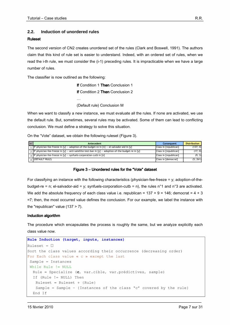
On the “Vote” dataset, we obtain the following ruleset (Figure 3).

N° Antecedent Consequent Distribution

1 IF physician-fee-freeze in [y] -- adoption-of-the-budget-re in [n] -- el-salvador-aid in [y] Class in [republican] (137; 4)

2 IF physician-fee-freeze in [y] -- anti-satellite-test-ban in [y] -- adoption-of-the-budget-re in [y] Class in [republican] (17; 0)

3 IF physician-fee-freeze in [y] -- synfuels-corporation-cutb in [n] Class in [republican] (9; 3)

4 (DEFAULT RULE) Class in [democrat] (5; 261)

Figure Figure Figure Figure 3333 –––– Unordered rules for the “Vote” datasetUnordered rules for the “Vote” datasetUnordered rules for the “Vote” datasetUnordered rules for the “Vote” dataset

For classifying an instance with the following characteristics (physician-fee-freeze = y; adoption-of-the-budget-re = n; el-salvador-aid = y; synfuels-corporation-cutb = n), the rules n°1 and n°3 are activated. We add the absolute frequency of each class value i.e. republican = 137 + 9 = 146; democrat = 4 + 3

=7; then, the most occurred value defines the conclusion. For our example, we label the instance with the "republican" value (137 > 7).

Induction algorithmInduction algorithmInduction algorithmInduction algorithm

The procedure which encapsulates the process is roughly the same, but we analyze explicitly each class value now.

Rule Induction (target, inputs, instances)

Ruleset = ∅

Sort the class values according their occurrence (d ecreasing order)

For Each class value « c » except the last

Sample = Instances

While Rule != NULL

Rule = Specialize ( c, var.cible, var.prédictives, sample)

If (Rule != NULL) Then

Ruleset = Ruleset + {Rule}

Sample = Sample – {Instances of the class “c” cov ered by the rule}

End If



End While

End For

Instances = Instances – {Instances covered for at l east one rule}

Ruleset = Ruleset + {Default rule (instances)}

Return (Ruleset)

The approach can handle a multiclass problem. The “specialize” procedure plays also an important role during the process. Specialize (class, target, inputs, instances) Rule = NULL Max.Measure = - ∞ Repeat Ref.Measure = - ∞ Proposition* = NULL For Each Candidate Proposition Measure = Evaluation (class, Rule, Proposition) If (Measure > Ref.Measure) Then Ref.Measure = Measure Proposition* = Proposition End If End For If (Ref.Measure > Max.Measure) Rule = Rule x Proposition* Max.Measure = Ref.Measure End If Until (Proposition* == NULL) If Significant (Rule) == TRUE Then Return(Rule) Else Return(NULL)

"Specialize" is a hill climbing optimization process. But, compared with the decision list approach, we try to discover the best rule for a specific value "class" of the target attribute.

Here again, the "evaluation" function is used to check the validity of a rule i.e. the support of the rule is

larger than the “Min.Support” parameter (10 by default). But it is used also to quantify the relevance of the rule. The goal of the optimization process is discover the most relevant rule.

In order to outline the various measures, we use the following cross-tabulation.

Premise Non (Premise) Total

Conclusion [Obs. ∈ class] acn cn

Conclusion [Obs. ∉ class]

Total an n

Where:

• n is the total number of instances sent to the procedure;

• an is the number of instances covered by the premise of the rule;

• cn is the number of positive (target value is “class”) instances sent to the procedure;

• acn is the number of positive instances covered by the rule;

• c

ac

n

n is the confidence of the rule, it states the purity of the rule.



Tanagra uses three measures. We ordered them according their ability to induce more specialized

rules. The behavior of the last one can be adjusted by using a certain parameter.

• Confidence statistic

( )( )1

/)(/)(

/),(

−−−

−=

n

nnnnnnnn

nnnnacZC

ccaa

caac

• Counter-examples statistic (Lerman, Gras and Rostam (1981 -- http://msh.revues.org/document2213.html)

n

nnn

nnnnnnacZI

ac

acaca

)(

/)()(),(

−−−−

−=

• Asymmetric J-Measure,

−−

−−

−×

=a

acc

a

acc

a

ac

a

aca

nn

nn

nn

nn

n

n

n

n

n

nacJ loglog),(

1

β

β

Compared to the standard J-Measure, the Asymmetric J-Measure ),( acJ β favors the over

representation of the class value "c" in the rule. In addition, the measure is parameterized by the weight β . When we increase β , we favor the more specialized rules. It seems that 4=β is a good

compromise between the support and the confidence of the induced rules.

The first two measures (ZI and ZC) are a test statistic comparing the initial target values distribution and conditional distribution. We can evaluate if the deviation is significant according to a statistical hypothesis schema. The "significant" procedure compares then the p-value of the test with a predefined threshold (Signif.Level = 0.05 if the default value). Actually, this procedure is mainly used

as a pre-pruning rule during the process. When we decrease the threshold, we obtain a shorter rule (the number of conditions into the premise is lower), and thus a classifier with fewer rules.

Numerical exampleNumerical exampleNumerical exampleNumerical example

We compute the various measures on the first rule (n°1) generated on the "Vote" dataset (Figure 3). We set 20=β in order to favor the confidence of the rules. We have the following cross-tabulation.

antecedent uncovered Rootrepublican (c) 137 31 168democrat (not c) 4 263 267Total 141 294 435

ZC (c,a) 17.3472 p-value 0

ZI (c,a) 8.8730 p-value 0

J20(c,a) 0.2853



Comparing the value of the various measures on the same rule is not very interesting. We observe

only that the rule seems relevant according the ZI and ZC measures (p-level < Signif. level = 0.05).

We detail here the computation of the Asymmetric J-Measure.

2853.0

294

31log

294

31

141

137log

141

137

435

141

loglog),(

20

1

1

=

−×

=

−−

−−

−×

=a

acc

a

acc

a

ac

a

aca

nn

nn

nn

nn

n

n

n

n

n

nacJ

β

β

More interesting is to analyze of the values of each measure through the path from the root (initial distribution) to the leaf during the search process.

In comparison of the rule defined by the leaf of the search path (Rule n°1 in the classifier - Figure 3), the rule defined by the only one condition (physician-fee-freeze = y) has the following characteristics

R1’: IF Physician-Fee-Freeze = y THEN Class = Republican (163; 14)

The confidence of the rule is lower (92% vs. 97%), but the support is larger (177 instances vs. 141).

When we compute the various measures

antecedent' uncovered Rootrepublican (c) 163 5 168democrat (not c) 14 253 267Total 177 258 435

ZC (c,a') 18.9500 p-value 0

ZI (c,a') 9.0799 p-value 0

J20(c,a') 0.0007

Definitely, the first two measures ZI and ZC prefers the simpler rule R1’ [ZC(a’,c) = 18.95 > ZC(a,c) = 17.35 ; ZI(a’,c) = 9.08 > ZI(a,c) = 8.87]; while the Asymmetric J-Measure, because we favors the rules with high confidence (we recall that we set 20=β ), favors the more complex rule R1 [J20(a’,c) =

0.0007 < J20(a,c) = 0.2853].



2.3. The other rule induction algorithms

In the two sections above, we outlined two very simple approaches, which are variants of the CN2 algorithm. We try to highlight the influence of the parameters on the characteristics of the obtained classifier (number of rules, support and confidence of the rules). Of course, there are many other algorithms. In an excellent survey, Furnkranz (1999) describes up to 40 algorithms. The most popular

is maybe the RIPPER method (Cohen, 1995 - http://www.cs.cmu.edu/~wcohen/), which is available under the JRIP appellation into the Weka software.

3. Dataset

In a marketing campaign, we want to detect the people which are interested by a new product. We have a binary target attribute (positive = yes; negative = no). The predictive attributes are the

customers’ characteristics (age, credit card, etc.). We have 79,838 instances (39.874 positive and 39.964 negative)7. We want to use the half of the dataset for the learning set, and the others for the test set.

4. Rule induction with Tanagra

4.1. Importing the database

After the launching of Tanagra, we create a new diagram by clicking on the FILE / NEW menu. We import the LIFE_INSURANCE.TXT data file.

7 http://eric.univ-lyon2.fr/~ricco/tanagra/fichiers/life_insurance.zip; we have the dataset into CSV (tab

separator) and ARFF (Weka) formats.



We want to subdivide the dataset into a learning sample (50%) and a test sample. We use the

SAMPLING component (INSTANCE SELECTION tab).

We set now “target” as TARGET attribute and the others as INPUT ones using the DEFINE STATUS component.



4.2. Induction of Decision Lists

We add the DECISION LIST component into the diagram. We click on the SUPERVISED PARAMETERS menu, the J-MEASURE is the default measure.

We validate these settings and we click on the VIEW menu. We obtain 20 rules in 156 ms.



In order to compute the test error rate, we add again the DEFINE STATUS component, we set “target”

as TARGET, and the prediction of the classifier as INPUT (PRED_SPVINSTANCE_1).

The prediction is computed for all the instances, including the test set. We add the TEST component

(SPV LEARNING ASSESSMENT tab) into the diagram. It computes automatically the error rate on the unselected instances i.e. the test set. We click on the VIEW menu. The error rate is 25.3%.



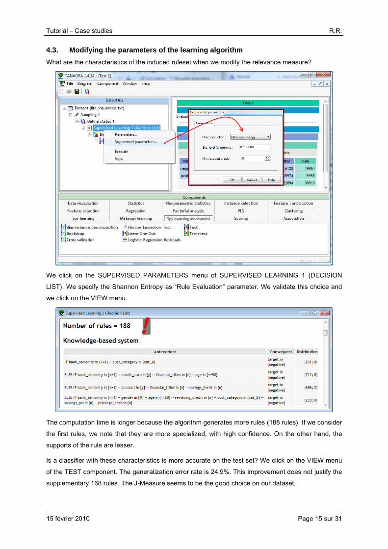
4.3. Modifying the parameters of the learning algorithm

What are the characteristics of the induced ruleset when we modify the relevance measure?

We click on the SUPERVISED PARAMETERS menu of SUPERVISED LEARNING 1 (DECISION

LIST). We specify the Shannon Entropy as “Rule Evaluation” parameter. We validate this choice and we click on the VIEW menu.

The computation time is longer because the algorithm generates more rules (188 rules). If we consider the first rules, we note that they are more specialized, with high confidence. On the other hand, the supports of the rule are lesser.

Is a classifier with these characteristics is more accurate on the test set? We click on the VIEW menu

of the TEST component. The generalization error rate is 24.9%. This improvement does not justify the supplementary 168 rules. The J-Measure seems to be the good choice on our dataset.



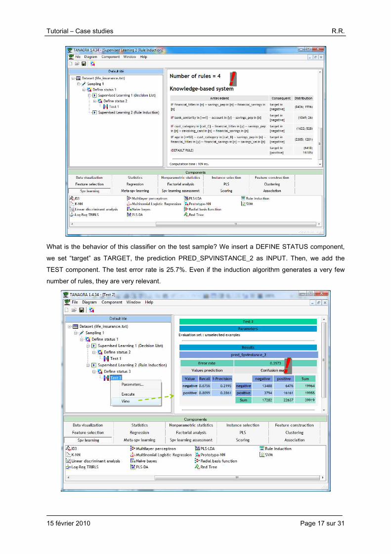
4.4. Induction of unordered rules

We use the RULE INDUCTION component (SPV LEARNING tab) in order to generate a set of unordered rules. We click on the SUPERVISED PARAMETERS menu, the default settings are the following.

We validate them. We click on the VIEW menu. We obtain only (!) 4 rules in 109 ms.



What is the behavior of this classifier on the test sample? We insert a DEFINE STATUS component,

we set “target” as TARGET, the prediction PRED_SPVINSTANCE_2 as INPUT. Then, we add the TEST component. The test error rate is 25.7%. Even if the induction algorithm generates a very few number of rules, they are very relevant.



5. Rule induction with Sipina

SIPINA includes several techniques for inducing rules. It implements for instance the hill-climbing version of the two original CN2 algorithms (1989 and 1991 papers).

Other induction algorithms are also implemented, such as the famous IREP approach (Furnkranz and Widmer, 1994)8 which is the ancestor of RIPPER (Cohen, 1995).

NoteNoteNoteNote: Make sure you use the 3.3 version for this tutorial. The version number is showed in the title bar of SIPINA.

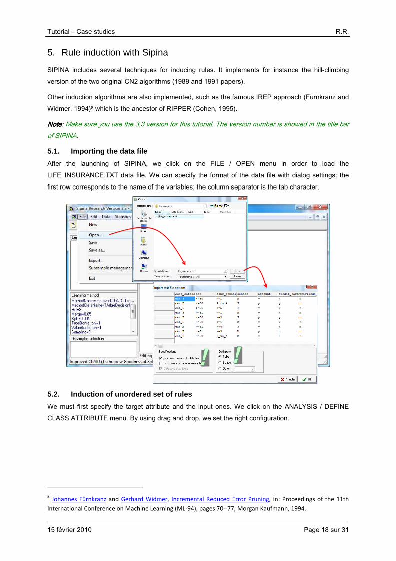
5.1. Importing the data file

After the launching of SIPINA, we click on the FILE / OPEN menu in order to load the LIFE_INSURANCE.TXT data file. We can specify the format of the data file with dialog settings: the

first row corresponds to the name of the variables; the column separator is the tab character.

5.2. Induction of unordered set of rules

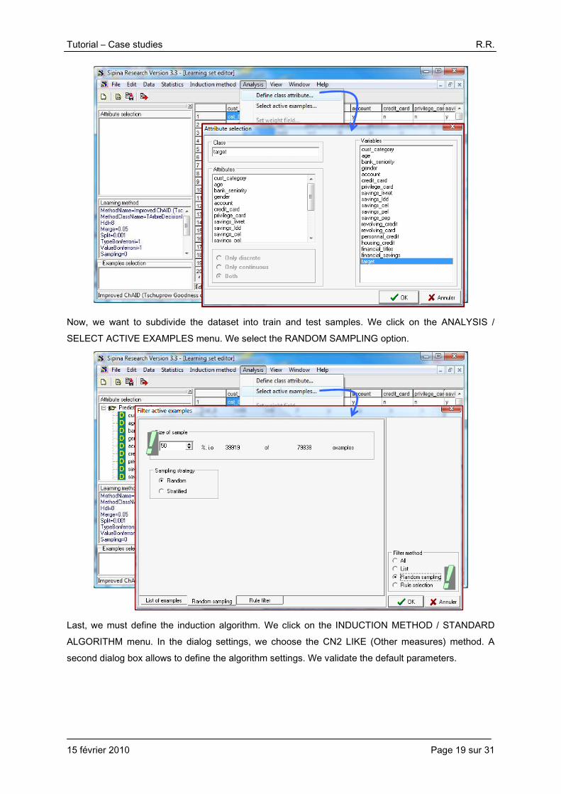
We must first specify the target attribute and the input ones. We click on the ANALYSIS / DEFINE CLASS ATTRIBUTE menu. By using drag and drop, we set the right configuration.

8 Johannes Fürnkranz and Gerhard Widmer, Incremental Reduced Error Pruning, in: Proceedings of the 11th

International Conference on Machine Learning (ML-94), pages 70--77, Morgan Kaufmann, 1994.



Now, we want to subdivide the dataset into train and test samples. We click on the ANALYSIS / SELECT ACTIVE EXAMPLES menu. We select the RANDOM SAMPLING option.

Last, we must define the induction algorithm. We click on the INDUCTION METHOD / STANDARD ALGORITHM menu. In the dialog settings, we choose the CN2 LIKE (Other measures) method. A second dialog box allows to define the algorithm settings. We validate the default parameters.



Now, we can launch the analysis by clicking on the ANALYSIS / LEARNING menu.

We obtain 4 rules which are very similar to those of Tanagra. It is not really surprising. The underlying algorithm is the same, but we do not sort the target values according to their occurrence here.

For each rule, SIPINA displays the support, the confidence and the lift. Because we have an unordered set of rules, we can sort them according one of these relevance indicators by clicking on

the header of the column.



Then, we want to assess the classifier. We click on the ANALYSIS / TEST menu. We choose the

“Inactive Examples of the Database” option in order to apply the rules on the test set. The test error rate is 25.71%.

5.3. Other rule induction algorithms with SIPINA

SIPINA incorporates other rule induction algorithms. We can analyze an approach which is very similar to CN2 for instance (CN2 de Clark et Boswell, 1991 – beam width = 1). We stop the current analysis by clicking on the ANALYSIS / STOP LEARNING menu. Then we select a new method into the method selection dialog box (INDUCTION METHOD / STANDARD ALGORITHM � RULE INDUCTION). We launch a new analysis (ANALYSIS / LEARNING menu). We obtain 166 rules. There

are many specialized rule, with a confidence close to 1.

Obtaining many rules does not mean a better performance. When we apply the classifier on the test set, the error rate is 30.9% (ANALYSIS / TEST � INACTIVE EXAMPLES OF DATABASES). There is certainly an overfitting phenomenon when the support of the rules is too low.



6. Rule induction with Weka

We use the 3.6.0 version of Weka (http://www.cs.waikato.ac.nz/ml/weka/). We perform the analysis with the explorer mode. I had to increase the "max heap size" to achieve the treatments described in this tutorial (see RUNWEKA.INI).

6.1. Importing the data file

We use the ARFF (Weka) file format. After the launching of Weka, we select the explorer mode, and

we load the data file by clicking on the OPEN FILE button. We pick the LIFE_INSURANCE.ARFF file.

By default, the last column corresponds to the target attribute. The organization of our data file is complying with that.



6.2. JRIP rule induction algorithm

JRIP seems very similar to the very popular RIPPER approach (Cohen, 1995). We activate the CLASSIFY tab, and we pick JRIP (CLASSIFIER / CHOOSE).



We use the hold-out evaluation process, the test set size corresponds to 50% of the whole dataset

(Test Options � Percentage Split = 50%).

JRIP creates an unordered set of 26 rules. Because JRIP implements a very sophisticated post-processing techniques in order to pruning each rule and the ruleset, the calculation time is longer (393.5 sec.). The test error rate is 25.8%.

6.3. Other rule induction algorithms with Weka

Weka includes many rule induction algorithms which are unobtainable elsewhere. In addition, each method is referenced by a published article in journals or in proceedings. This is really impressive.

PARTPARTPARTPART (Frank et Witten, « Generating Accurate Rule Sets without Global Optimization », in 15th ICML, 144-151, 1998). It induces a decision list. It seems that the algorithm is a combination of C4.5 and

RIPPER. We select this method and we click on the START button.

We obtain 1228 rules and the test error rate is 24.8%.

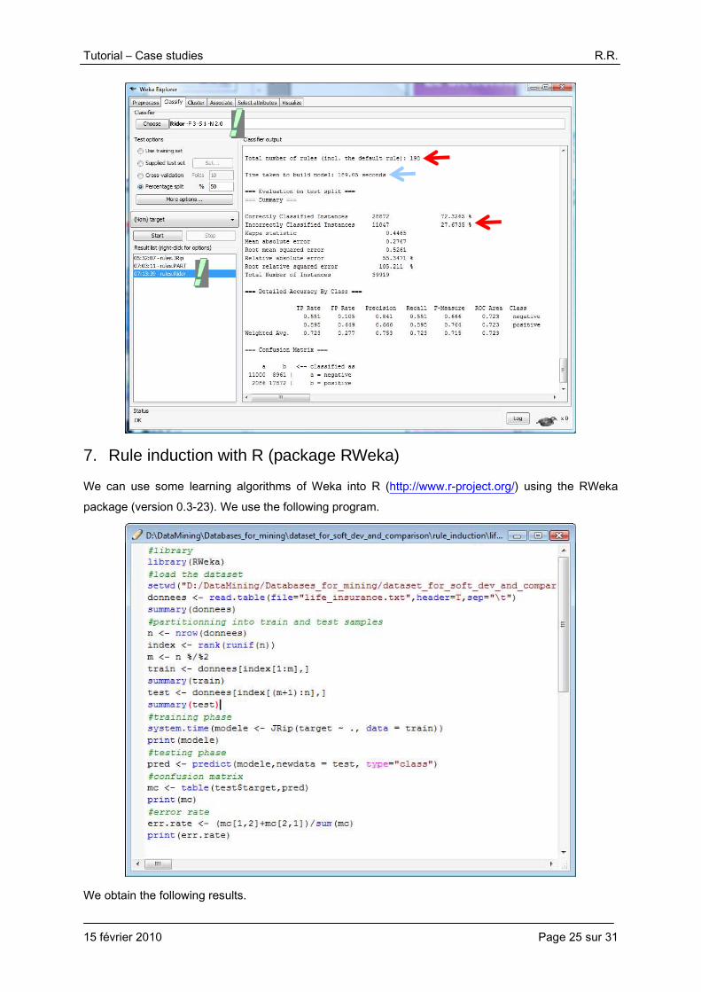
RIDORRIDORRIDORRIDOR (Gaines et Compton, « Induction of Ripple Down Rules Applied to Modeling Large Databases », in Journal of Intelligent Information Systems, 5(3), 211-228, page 1995). It generates a default rule first and then the exceptions for the default rule with the least (weighted) error rate. Then it generates the “best” exceptions for each exception and iterates until pure. Thus it performs a tree-like expansion of exceptions. The exceptions are a set of rules that predict classes other than the default.

IREP is used to generate the exceptions (http://mydatamining.wordpress.com/2008/04/14/rule-learner-or-rule-induction/).

We obtain 198 rules with a test error rate of 27.7% with RIDOR.



7. Rule induction with R (package RWeka)

We can use some learning algorithms of Weka into R (http://www.r-project.org/) using the RWeka package (version 0.3-23). We use the following program.

We obtain the following results.



We obtain 29 rules, and the test error rate is 25.7%. Because we had partitioned randomly the

dataset, it is natural that we obtain slightly different results than Weka. More surprisingly (?), the procedure is significantly faster under R (85.7 sec. against 393.5 sec. under Weka).

8. Rule induction under RapidMiner

RapidMiner (http://rapid-i.com/content/view/181/190/) incorporates various rule induction algorithms. We can also import the learning methods from Weka. We define the following diagram.

We use the following settings:

• ARFF EXAMPLE SOURCE loads LIFE_INSURANCE.ARFF. We state the target attribute (LABEL_ATTRIBUTE = target).



• SIMPLE VALIDATION allows to subdivide the dataset. We set SPLIT_RATIO = 0.5. I do not know

how to display the rules computed on the training set only. We selection the CREATE COMPLETE MODEL option in order to obtain the rules computed on the whole dataset.

• RULE LEARNER is the learning method. It seems very similar to RIPPER. • CLASSIFICATION PERFORMANCE computes the test error rate (CLASSIFICATION ERROR).

We click on the RUN button. In the first tab, we obtain the test error rate (28.64%).

Into the second tab, we have the ruleset, we obtain 23 rules.



About the computation time, it is 2.23 minutes for the whole process. The creation of the ruleset on the

training set seems to take 55 seconds.

9. Rule induction with Orange

Orange (http://www.ailab.si/orange/) incorporates the CN2 algorithm. There is a little variation of the original algorithm however. We define the following scheme.

DATA SAMPLER enables to subdivide the dataset (RANDOM SAMPLING – SAMPLE SIZE = 50%) We select the WRACC measure into the CN2 component. It allows to obtain less specialized rules, and thus less numerous rules.

The induced ruleset can be viewed into the CN2 RULE VIEWER component. We have 4 rules. The calculation time is about 30 seconds. The test error rate is 28.5%.



10. Comparison of the implemented algorithms

We outline the main results into the following table, sorted according the test error rate:

Approach # rules Test Error Rate (%) Calculation time (sec.)WEKA / PART 1228 24.8 126.1TANAGRA / DECISION LIST (Shannon) 188 24.9 2.3TANAGRA / DECISION LIST (J-Measure) 20 25.3 0.2R / JRIP (Package Rweka) 29 25.7 89.7SIPINA / CN2 Like (Mis.Rate Stat) 4 25.7 0.9TANAGRA / RULE INDUCTION (Mis.Rate Stat) 4 25.7 0.1WEKA / JRIP 26 25.8 393.5WEKA / RIDOR 198 27.7 189.1ORANGE / CN2 (WRACC measure) 4 28.5 30.0RAPID MINER / RULE LEARNER 23 28.6 55.0

Ruleset characteristics

We observe that:

• The fewer is the number of generated rules, the faster is the algorithm. It is not really surprising. • The generalization error rate is similar (about 27%) whatever the method. • A simple classifier with a few rules can be as accurate as a complex classifier. This result is often

noted when we perform an analysis on real datasets.

Of course, we can obtain better results if we fine-tune the settings of the algorithms. But getting the appropriate values is not always obvious. It depends on the learning algorithm and the dataset characteristics.



11. Comparison with the decision tree induction

We want to compare the performances of the rule based classifier with the decision tree. We used the C-RT component (CART – Breiman and al., 1984). We obtain the following tree in 500 ms.

We obtain 29 rules since there are 29 leaves. The test error rate is 25.6%. These values are similar to those obtaining with the rule induction methods. It is not surprising. Many experiments of various

databases give the same conclusion (e.g. http://data-mining-tutorials.blogspot.com/2008/11/decision-lists-and-decision-trees.html).



12. Conclusion

In this tutorial, we wanted to highlight the approaches for the induction of prediction rules. They are mainly available into academic tools from the machine learning community. We note that they are an alternative quite credible to decision trees and predictive association rules, both in terms of accuracy than in terms of processing time.

tanagra rule induction -...

Documents