tampere university of technology - tutmuvis.cs.tut.fi/documents/mscthesispartio.pdf · tampere...
TRANSCRIPT

TAMPERE UNIVERSITY OF TECHNOLOGY Department of Electrical Engineering Institute of Signal Processing
Mari Partio
Content-based Image Retrieval using Shape and Texture Attributes
Master of Science Thesis
Subject approved in the Department Council meeting on 10 April 2002
Examiners: Professor Moncef Gabbouj Researcher Bogdan Cramariuc

Preface This Thesis has been carried out in the Institute of Signal Processing, Tampere University
of Technology, Finland. The work is part of the MuVi-project, whose emphasis is on
content-based image and video retrieval. First, I would like to thank my examiners,
Professor Moncef Gabbouj and Researcher Bogdan Cramariuc for their corrections and
guidance towards finishing this thesis. I would also like to give special thanks to whole
Image and Video Analysis group. I would also like to thank SPAG and Academy of
Finland for their financial support. Last but not least, I would like to dedicate special
thanks to my family and friends for their continuous support during this work.
Tampere 19.11.2002, Mari Partio Vaajakatu 5 H 176 33720 Tampere, Finland Mobile: 040-7323079 Email: [email protected]
2

Contents
Preface..............................................................................................................2 Contents ...........................................................................................................3 Abstract............................................................................................................5 Tiivistelmä........................................................................................................6 Symbols and Abbreviations ...........................................................................8 1 Introduction ........................................................................................... 11 2 Content-based Image Retrieval (CBIR) .............................................. 14
2.1 The Problem of Content-based Retrieval ................................................... 14 2.2 Feature Extraction........................................................................................ 15
2.2.1 Color………………………………………………………………15 2.2.2 Shape……………………………………………………………...16 2.2.3 Texture…………………………………………………………….16 2.2.4 Spatial layout……………………………………………………...16
2.3 Similarity models .......................................................................................... 17 2.3.1 The metric model………………………………………………….17 2.3.2 Transformational distances………………………………………..18 2.3.3 Tversky’s model…………………………………………………..18
2.4 Indexing ......................................................................................................... 18 2.5 Example CBIR system: MUVIS .................................................................. 19 2.6 MPEG-7 ......................................................................................................... 21
2.6.1 Overview of MPEG-7 …………………………………………….21 2.6.2 Shape features …………………………………………………….22 2.6.3 Texture features…………………………………………………...24
3 Human Visual Perception..................................................................... 26 3.1 Anatomy of the human eye .......................................................................... 26 3.2 Lateral Inhibition.......................................................................................... 27 3.3 Perception of Shape ...................................................................................... 28
3.3.1 Classical theories of shape perception…………………………… 28 3.3.2 Modern theories of shape perception …………………………… 29
3.4 Perception of Texture ................................................................................... 29 3.4.1 Feature approach………………………………………………… 29 3.4.2 Frequency approach……………………………………………... 30
4 Shape Analysis ....................................................................................... 31 4.1 Introduction to Shape................................................................................... 31 4.2 Shape Attributes ........................................................................................... 32
4.2.1 Region-based attributes…………………………………………...32 4.2.2 Boundary-based attributes………………………………………...35 4.2.3 Multi-resolution attributes………………………………………...37
3

4.3 Shape Correspondence using Ordinal Measures....................................... 40 4.3.1 Object alignment based on universal axes………………………..40 4.3.2 Boundary to multilevel image transformation……………………42 4.3.3 Similarity evaluation……………………………………………...44
4.4 Experiments using Ordinal Correlation..................................................... 46 4.4.1 Introducing dataset and selected parameters……………………...46 4.4.2 Results and their evaluation………………………………………47
5 Texture Analysis .................................................................................... 49 5.1 Introduction to Texture................................................................................ 49 5.2 Texture Attributes ........................................................................................ 50
5.2.1 Spatial Methods…………………………………………………...50 5.2.2 Frequency-based methods………………………………………...51 5.2.3 Moment-based methods…………………………………………..52
5.3 Co-occurrence matrix................................................................................... 55 5.3.1 Introduction……………………………………………………….55 5.3.2 Description of the Selected Features……………………………...55
5.4 Gabor filters .................................................................................................. 56 5.4.1 Gabor function…………………………………………………….56 5.4.2 Gabor filter bank desing…………………………………………..57 5.4.3 Feature Representation……………………………………………58
5.5 Experiments................................................................................................... 58 5.5.1 Testing Database………………………………………………….59 5.5.2 Retrieval Procedure……………………………………………….60 5.5.3 Retrieval Results…………………………………………………..61 5.5.4 Evaluation of the Results………………………………………….62 5.5.5 Comparison with Gabor Results…………………………………..62
6 Conclusions ............................................................................................ 66 References ..................................................................................................... 68
4

Abstract TAMPERE UNIVERSITY OF TECHNOLOGY Degree Program in Electrical Engineering Institute of Signal Processing Partio, Mari: Content-based Image Retrieval using Shape and Texture Attributes Master of Science Thesis, p. 70 Examiners: Professor Moncef Gabbouj, Researcher Bogdan Cramariuc Funding: Center of Excellence, SPAG, Academy of Finland Department of Electrical Engineering November 2002 Due to rapid increase in volume of image and video collections, traditional methods of indexing and retrieval using only keywords have become outdated. Therefore, alternative methods to describe images using their visual content have been developed. To produce and test algorithms for content-based image and video retrieval, MUVIS (Multimedia Video Indexing and Retrieval System) was developed at TUT. The goal of MUVIS is a fast, real-time and reliable audio/video (AV) browsing and indexing application, which is also capable of extracting some key features (such as color, texture and shape) of the AV media. Most of the existing image retrieval systems perform reasonably when using color features. However, retrieval accuracy using shape or texture features does not produce as good results. Therefore, this thesis investigates different methods of representing shape and texture in content-based image retrieval. Later, when appropriate segmentation algorithms are available some of these methods could also be applied to video object retrieval. The thesis presents two contributions: one is shape-based and the second is texture-based retrieval method. The former contribution concerns shape analysis and retrieval. Shape attributes can be roughly divided into two main categories: boundary-based and region-based. Since the human visual system itself focuses on edges and ignores uniform regions, this thesis concentrates on boundary-based representations. A novel boundary-based method using distance transformation and ordinal correlation is developed in this thesis. Simulation results show that the proposed technique produced encouraging results when using MPEG-7 shape test database. The second contribution of the thesis is a constrained application in which the database contains a set of rock images. In this application, we applied a technique based on Gray-Level Co-occurrence matrices (GLCM) and compared the results with a well-known method from the literature. It was found that GLCM outperforms Gabor Wavelet features when considering retrieval time and visual quality of the results.
5
Tiivistelmä TAMPEREEN TEKNILLINEN KORKEAKOULU Sähkötekniikan koulutusohjelma Signaalinkäsittelyn laitos Partio, Mari: Kuvan hakeminen käyttäen muoto- ja tekstuuriattribuutteja Diplomityö, s. 70 Tarkastajat: prof. Moncef Gabbouj, tutkija Bogdan Cramariuc Rahoitus: SPAG, Suomen Akatemia Sähkötekniikan osasto Marraskuu 2002 Digitaalisten kuva- ja videokokoelmien nopea kasvu on johtanut tehokkaiden selain- ja hakuohjelmistojen kehittämiseen. Perinteiset kuvanhakumenetelmät perustuvat manuaalisesti lisättyihin kuvaa kuvaaviin avainsanoihin, joiden ongelmana on subjektiivisuus sekä tietokantojen kasvusta johtuva työläys. Tästä syystä vaihtoehtoisten kuvan visuaalisiin ominaisuuksiin, esimerkiksi väriin, tekstuuriin ja muotoihin, pohjautuvien menetelmien kehittäminen kuvien sisällön esittämiseksi on yhä tärkeämpää. Sisältöpohjaisessa kuvanhaussa (CBIR) on tavoitteena löytää tietokannasta visuaalisilta ominaisuuksiltaan hakukuvaa (query image) mahdollisimman hyvin vastaavat kuvat. Ensin kuvista irrotetaan tärkeimmät piirteet ja ne tallennetaan ominaisuusvektoreihin (feature vector). Ominaisuusvektorit indekseineen tallennetaan tietokantaan. Hakukuvan ominaisuusvektoria verrataan muiden kuvien ominaisuusvektoreihin valittua etäisyysmittaa (similarity metric) käyttäen ja kuvat palautetaan etäisyyksien mukaan järjestyksessä pienimmästä alkaen. CBIR -järjestelmien yleistyessä yhtenäisten standardien luominen on tullut yhä tärkeämmäksi. MPEG-7 on MPEG:n (Moving Picture Experts Group) kehittämä standardi, jonka tarkoituksena on kuvata multimediadatan sisältöä. MPEG-7 keskittyy informaation tarkoituksen ja sisällön tulkintaan ja sen vuoksi se on avainasemassa sisältöpohjaisten hakujärjestelmien kehittämisessä. Tämä diplomityö on osa Tampereen Teknillisen Korkeakoulun signaalinkäsittelyn laitoksella kehitettävää MUVIS -järjestelmää, jonka tavoitteena on tuottaa nopea, reaaliaikainen ja luotettava audio/video (AV) multimediahakuohjelmisto, joka pystyy myös poimimaan avainominaisuuksia AV mediasta. Tässä työssä keskitytään lähinnä kuvahakuun, mutta videon segmentointiin käytettävien algoritmien kehittyessä esitettyjä menetelmiä voidaan käyttää myös videohakuun. Useat olemassa olevista kuvanhakujärjestelmistä ovat suorituskyvyltään kohtalaisia suoritettaessa haku väriominaisuuksien perusteella. Käytettäessä muotoa tai tekstuuria hakuperusteena tulokset ovat yleensä epätarkempia. Siksi tässä työssä keskitytään
6

tarkastelemaan erilaisia muotoa ja tekstuuria kuvaavia attribuutteja sekä niiden soveltuvuutta automaattiseen kuvanhakuun. Työ koostuu kahdesta osasta: muoto-pohjaisesta ja tekstuuri-pohjaisesta kuvanhakumenetelmästä. Ensimäisessä osassa käsitellään muodon analyysia ja hakua. Muotoattribuutit voidaan karkeasti jakaa kahteen pääluokkaan: reunapohjaiseen sekä aluepohjaiseen. Koska ihmisen näköaisti keskittyy reunoihin ja jättää tasaiset alueet vähemmälle huomiolle, tässä työssä keskitytään reunapohjaiseen esitystapaan. Etuna reunapohjaisissa menetelmissä on myös se, että ne kuvaavat muotoa tarkemmin ja mahdollistavat muodon kuvaamisen useammalla resoluutiolla (multiresolution approach). Työssä kehitetään myös uusi reunapohjainen muotojen vertailumenetelmä, joka perustuu etäisyysmuunnokseen (distance transformation) sekä ”ordinal correlation–menetelmään”. Esitetty menetelmä antoi rohkaisevia tuloksia MPEG-7:n testidatalla testattaessa. Työn toisessa osassa esitellään tekstuuripohjainen kivikuvien samankaltaisuuden vertailuun keskittyvä sovellus. Tarkkaa määritelmää tekstuurille ei ole, mutta yleensä tekstuurilla käsitetään kuvan aluetta, joka koostuu samankaltaisista toistuvista elementeistä. Riiipuen näiden peruselementtien järjestyksestä, tekstuuria voidaan karkeasti pitää joko säännöllisenä tai stokastisena. Koska tässä työssä käytetyt kivikuvat ovat luonteeltaan stokastisia, tilastolliset menetelmät soveltuvat niiden kuvaamiseen parhaiten. Käytetty tekniikka (GLCM) on tunnettu ja perustuu harmaasävyjen suhteelliseen esiintymiseen kuvassa. Verrattaessa saatuja tuloksia ”Gabor –suodinpankilla” saatuihin, voidaan havaita GLCM paremmaksi tarkasteltaessa hakuaikaa sekä hakutulosten visuaalista laatua.
7
Symbols and Abbreviations Symbols: A area of a region, p. 32 Anl orthogonal Zernike moment of order n and repetition l, p. 53 Ck position of the contour pixel k in the image G, p. 43 dx distance in x-direction, p. 55 dy distance in y-direction, p. 55 Dj metadifference obtained by calculating distance between all pairs of metaslices, p.45 E[N(L)] expected number of boxes, p. 51 fDC mean intensity of texture, p. 24 fSD standard deviation of texture, p. 24 f(x,y) continuous 2D function, p.33 F(n) Discrete Fourier Transform of u(k), p. 36 G gray-scale image, p. 42 Gi pixel values of G, p. 42 g(u,σ) 1D Gaussian kernel of width σ, p. 38 g(x,y) 2D Gabor function, p. 57 G(u,v) Fourier transform of 2D Gabor function, p. 57 I(x,y) image, p. 50 K number of boundary samples, p. 36 l1 number of universal axes, p. 41 L1 histogram distance, p. 15 L2 histogram intersection, p.15 mpq moment of order (p+q), p. 33 M(n) magnitude of the Fourier Descriptors, p. 36 Mk moment image, p. 53 Mpq central moment, p. 34 Mj
X metaslice obtained by combining slices SkX, p. 45
MjY metaslice obtained by combining slices Sk
Y, p. 45 N number of contour points, p. 33 P perimeter of a contour, p. 32 Pd co-occurrence matrix using distance d, p. 55 Qp(σ) radial polynomial of the OFM, p. 54 Rj
X contains the pixels from image X, which belong to area Rj, p. 44 Rj
Y contains the pixels from image Y, which belong to area Rj, p. 44 Rnl radial polynomial for Zernike moments, p. 54 s1, s2, s3 generic stimuli, p. 17 Sk
X slice constructed for every pixel Xk in image X, p. 44
SkY slice constructed for every pixel Yk
in image Y, p. 45
TD feature vector of the HTD, p. 24 u(k) sequence of coordinates (x(k), y(k)) of K-point digital contour in the
xy-plane, k=0, 1, 2, …, K-1, p. 36 û(k) u(k), but only the first M coefficients used, p. 36 Uh higher central frequency, p. 57
8

Ul lower central frequency, p. 57 Upq basis function of the OFM, p. 54 V0 value on the contour, p. 43 Vnl(x,y) Zernike basis function of order n and repetition l, p. 54 W window width for calculating moments, p. 52 Wmn Gabor Wavelet transform, p. 58 xc x-coordinate of the centroid, p. 34 xm normalized x-coordinate for the moment calculation, p. 52 xpyq basis function in geometric moments definition, p. 54 yc y-coordinate of the centroid, p. 34 ym normalized y-coordinate for the moment calculation, p. 52 ηnq normalized definition of moments, p. 34 κ(u) curvature function for any parametrized contour, p. 38 κ(u,σ) evolved curve contour, p. 38 λ the sum of all metadifferences, p. 45 µmn mean value on a certain frequency band, p. 58 µr mean radius, p. 33 µ centroid of a region, p. 33 φ1-φ7 a set of seven invariant moments, p. 34 - 35 σ parameter that controls the shape of the logistic function, p. 53 σmn standard deviation on a certain frequency band, p. 58 ρ Spearman’s ρ (ordinal correlation coefficient), p. 45 ρ(x,y) autocorrelation function, p. 50 τ Kendall’s τ (ordinal correlation coefficient), p. 45
Γ(u) parametrized contour, p. 38 Θµ polar angle, p. 41 θj directional angle, p. 41 Abbreviations: 1D One-dimensional 2D Two-dimensional 3D Three-dimensional AV Audio-visual CBIR Content-based image retrieval CSS Curvature Scale-Space D Descriptor (MPEG-7 standard) DFT Discrete Fourier Transform DDL A Descriptor Definition Language (MPEG-7 standard) DS Description Scheme (MPEG-7 standard) FD Fourier Descriptor GLCM Gray-level co-occurrence matrix H.263+ ITU-T standard HCP High Curvature Point HSV Color model (hue, saturation, value) HTD Homogeneous Texture Descriptor (MPEG-7 standard) ISO The International Organization for Standardization
9

MPEG-1 ISO standard MPEG-2 ISO standard MPEG-4 ISO standard MPEG-7 ISO standard MuVi Multimedia Video Indexing and Retrieval MUVIS Multimedia Video Indexing and Retrieval System NeTra CBIR system, University of California at Santa Barbara OFM Orthogonal Fourier-Mellon moment OR Ordinal correlation PC Personal computer Photobook CBIR system, MIT, Massachusetts Institute of Technology QBIC CBIR system designed by IBM® RGB Color model (red, green, blue) SQUID Shape Queries Using Image Databases (CBIR system, University of
Surrey, UK) TUT Tampere University of Technology UA Universal Axes VisualSEEK CBIR system, Columbia University WT Wavelet Transform WTMM Wavelet Transform Modulus Maxima
10

1 Introduction
During the last decade there has been a rapid increase in volume of image and video
collections. A huge amount of information is available, and daily gigabytes of new visual
information is generated, stored, and transmitted. However, it is difficult to access this
visual information unless it is organized in a way that allows efficient browsing,
searching, and retrieval. Traditional methods of indexing images in databases rely on a
number of descriptive keywords, associated with each image. However, this manual
annotation approach is subjective and recently, due to the rapidly growing database sizes,
it is becoming outdated. To overcome these difficulties in the early 1990s, Content-Based
Image Retrieval (CBIR) emerged as a promising means for describing and retrieving
images. According to its objective, instead of being manually annotated by text-based
keywords, images are indexed by their visual content, such as color, texture, shape, and
spatial layout.
The importance of content-based retrieval for many applications, ranging from art
galleries and museum archives to picture collections, criminal investigation, medical and
geographic databases, makes the visual information retrieval one of the fastest growing
research fields in information technology. Therefore, many content-based retrieval
applications have been created for both research and commercial purposes. In the late
1990s – with the vast introduction of digital images and video to the market – the
necessity for interoperability among different applications that deal with AV content
description arose. For this purpose, in 1997 the ISO MPEG Group initiated the “MPEG-7
Multimedia Description Language” work item. As a goal of this activity, an international
11

1 Introduction
12
MPEG-7 standard was issued in July 2001, defining standardized descriptions and
description systems that allow users or agents to search, identify, filter, and browse
audiovisual content.
The MUVIS system [32], developed at TUT extracts the low level features, such as color,
texture, and shape. It evaluates similarity between a query image and all the other images
in the database specified by the user, and returns the most similar images as best matches.
There exist several systems and applications similar to MUVIS, such as QBIC [12], NeTra
[45], VisualSEEK (color&texture) [23], SQUID [19] and Photobook [6].
The aim of TUT MuVi is to develop a fast, real-time and reliable audio/video (AV)
browsing and indexing framework, which is also capable of extracting well-defined key
features of the AV media. This thesis concentrates on describing shape and texture
attributes, which are now applied on still images. Later, after efficient segmentation, they
should be applied also on video sequences.
Shape is one of the most important visual attributes in an image. In fact, the human visual
system is able to extract and abstract shapes from very complex scenes. The concept of
shape is invariant to translations, rotations, and scaling, the shape of an object is a binary
image representing the extent of the object. Due to these considerations shape presentation
is one of the most challenging aspects of computer vision. Shape representations can be
roughly classified in two major categories: boundary-based and region-based. The former
represents shape by its outline, while the latter considers shape being formed of a set of
two-dimensional regions. The human visual system itself focuses on edges and ignores
uniform regions. Therefore, this thesis is mostly concentrated on boundary-based
representations. On the other hand, feature vectors extracted from boundary-based
representations provide a richer description of a shape allowing the development of multi-
resolution shape description. In this thesis, we give short introduction to most well known
region-based, boundary-based and multi-resolution techniques. In addition, a recently
developed boundary-based approach on shape similarity estimation based on ordinal
correlation is presented.
1 Introduction
13
Texture is another important visual attribute, since it is present almost everywhere in
nature. Textures may be described according to their spatial, frequency or perceptual
properties. This thesis describes briefly several approaches to texture representation and
gives a more detailed view on one spatial representation method (co-occurrence matrices)
and one frequency based method (gabor filter). There is a multi-resolution approach
available for the former, but the latter is a multi-resolution approach by its nature.
In experiments using texture attributes we provide a constrained retrieval application in
which the database contains a set of rock images. In this application, we apply a technique
based on Gray-Level Co-occurrence matrices (GLCM) and compare the results with a
well-known method from the literature. Evaluation of the results is also provided.
This thesis is organized as follows. Chapter 2 reviews the idea behind content-based
retrieval. Chapter 3 gives an overview of the human visual system characteristics, which
play an important role in similarity assessment. Chapters 4 and 5 represent the core of this
thesis. Chapter 4 begins by introducing different shape attributes. It continues by
presenting a novel boundary-based method using distance transformation and ordinal
correlation. The chapter ends by providing some experimental results. Chapter 5 presents
different texture attributes used in content-based image retrieval. The chapter is concluded
by a constrained application in which gray-level co-occurrence matrices are applied to
retrieval of rock images. Chapter 6 provides the conclusions of this thesis.
2 Content-based Image Retrieval (CBIR)
2.1 The Problem of Content-based Retrieval
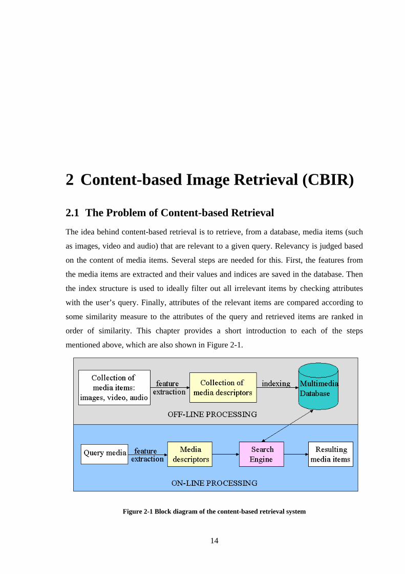
The idea behind content-based retrieval is to retrieve, from a database, media items (such
as images, video and audio) that are relevant to a given query. Relevancy is judged based
on the content of media items. Several steps are needed for this. First, the features from
the media items are extracted and their values and indices are saved in the database. Then
the index structure is used to ideally filter out all irrelevant items by checking attributes
with the user’s query. Finally, attributes of the relevant items are compared according to
some similarity measure to the attributes of the query and retrieved items are ranked in
order of similarity. This chapter provides a short introduction to each of the steps
mentioned above, which are also shown in Figure 2-1.
Figure 2-1 Block diagram of the content-based retrieval system
14

2.2 Feature Extraction
15
2.2 Feature Extraction
Feature extraction is one of the most important components in a content-based retrieval
system. Since a human is usually judging the results of the query, extracted features
should mimic the human visual perception as much as possible. In broad sense, features
may be divided into low-level features (such as color, texture, shape, and spatial layout)
and high-level semantics (such as concepts and keywords). Use of only low-level features
might not always give satisfactory results, and therefore, high-level semantics should be
added to improve the query whenever possible. High-level semantics can be either
annotated manually or constructed automatically from low-level features. In this chapter
the general low-level visual features are described.
2.2.1 Color
Color is one of the most widely used visual attributes in image retrieval. In fact, most
existing image retrieval systems such as QBIC [12], Netra [45], and VisualSEEK[23] are
most efficient in color retrieval. Retrieval by color similarity requires using such models
of color stimuli that distances in color space correspond to human perceptual distances
between colors. Studies by psychologists and artists have demonstrated that the presence
and distribution of colors induce sensations and convey meaning to the observer,
according to specific rules, which are explained in more detail in [3].
Color histogram is the most commonly used presentation. The histogram reflects the
statistical distribution, or the joint probability of the intensities of the three color channels.
The color histogram is computed by discretizing the colors within the image and counting
the number of pixels of each color. Chromatic similarity between the query histogram and
the histograms of the database images can be evaluated by computing the L1 and L2
distances [3]. L1 distance is a measure of histogram intersection, whereas a L2-related
metric takes into account the similarities between similar but not necessarily identical
colors [46].
Color stimuli are commonly represented as points in three-dimensional color spaces.
Before building the histogram the hardware-oriented (RGB) color space is usually
converted into some perceptually uniform color space, such as the HSV (hue, saturation,
2.2 Feature Extraction
16
value) space. Hue describes the actual wavelength of the color percept, saturation indicates
the amount of white light present in the color and brightness (value) represents the
intensity of the color.
2.2.2 Shape
The shape of an object is a binary image representing the extent of the object. Since the
human perception and understanding of objects and visual forms relies heavily on their
shape properties, shape features play a very important role in CBIR. In general the useful
shape features can be divided into two categories, boundary-based and region-based.
These representations will be introduced in Chapter 4, where two additional extensions for
boundary-based representations, multi-resolution approach and similarity evaluation based
on ordinal correlation, are presented.
2.2.3 Texture
Although no single formal definition for texture exists [33], we refer to texture as an area
containing variations of intensities, which form repeated patterns. Those patterns can be
caused by physical surface properties, such as roughness, or they could result from
reflectance differences, such as the color on a surface. Differences observed by visual
inspection are difficult to define in quantitative manner, which leads to the necessity of
defining texture using some features. In this thesis textural attributes are divided into three
categories: spatial, frequency and moment-based attributes [3]. Those properties will be
discussed in more detail in Chapter 5.
2.2.4 Spatial layout
Spatial relationships between entities often capture the most relevant information in an
image. However, defining similarity according to spatial relationships is generally
complex because relations are not represented by a single crisp statement but rather by a
set of contrasting conditions, which are concurrently satisfied with different degrees. In [3]
spatial relationships are divided into two categories: object-based and relational structures.
In object-based structures spatial relationships are not explicitly stored but visual
information is included in the representation. In this case images are retrieved using object
coordinates. Object-based structures are based on a space partitioning technique that
2.2 Feature Extraction
17
allows a spatial entity to be located in the space it occupies. Therefore, in image retrieval
systems, they can be employed in spatial queries concerned with finding a spatial entity
within the image space.
Relation based structures do not include visual information and preserve only a set of
spatial relationships discarding all uninteresting relationships. Objects are represented
symbolically and spatial relationships explicitly. In image retrieval systems, relation based
structures are suited for finding all images with objects in similar relationships as a query
image.
2.3 Similarity models
2.3.1 The metric model
In the metric model, it is assumed that a set of features models the properties of the input
object (stimulus) so that it can be presented as a point in a suitable feature space. If d is a
distance function and s1, s2, s3 are generic stimuli the following metric axioms must be
verified:
• constancy of self-similarity: ( ) ;3,2,10, == iforssd ii
• minimality: ;0),( jiforssd ji ≠≥
• symmetry property: ( ) ( ) ;3,2,1,,, == jiforssdssd ijji
• triangle inequality property: ( ) ( ) ( ) .3,2,1,,,,, =≥+ kjiforssdssdssd kikjji
Most commonly used distance functions are:
• the Euclidean distance: ( ) ( ) ;),( 212
21221 yyxxssd −+−=
• the city-block distance: ;),( 121221 yyxxssd −+−=
where s1=(x1 , y1) and s2=(x2 , y2).
The metric model has several advantages for similarity measurement. First, it is well
suited to very large image databases since an index can be build for the feature vectors to
speed up the retrieval response. Second, it is consistent with feature-based description.
However, many studies in psychology have pointed out certain inadequacies of the feature

2.3 Similarity models
18
vector model and metric distances to establish a reliable approach to mimic human
judgement of similarity [3].
2.3.2 Transformational distances
This approach is based on the idea that, in order to evaluate the similarity between shapes,
one shape is transformed into the other through a deformation process. Similarity between
shapes is then measured through the amount of deformation needed to make the two
shapes coincide. Two different models exist. Elastic models use either a discrete set of
parameters to model the deformation, or a continuous contour undergoing a continuous
deformation. Evolutionary models consider shapes as the result of a process in which, at
every step, forces are applied at specific points of the contour. Elastic models for retrieval
by shape similarity have been employed for example in Photobook [6].
2.3.3 Tversky’s model
Tversky’s model characterizes stimuli as a set of features but defines similarity according
to set-theoretic considerations. Similarity ordering is obtained as a linear combination of a
function of two types of features: features common to both stimuli and features belonging
to one stimulus and not to the other. The following theorem holds [3]: if p is a similarity
function, there is a similarity function P and a non-negative function f, so that for all
stimuli si and their respective set of features Si:
( ) ( ) ( ) ( )43214321 ,,,, sspsspssPssP >⇔> (2.1)
( ) ( ) ( ) ( )12212121 , SSfSSfSSfssP −−−−∩= βα (2.2)
The Tversky’s model assumes binary features, which act as predicates for certain stimulus.
The model accounts for several aspects of human similarity that are not covered by the
metric approach. However, this approach does not allow for easy indexing [3].
2.4 Indexing
When the number of images in the database is very large, there is a need for indexing
visual information to avoid sequential scanning. Index structures ideally filter out all
irrelevant images by checking image attributes with the user’s query. Therefore, only
relevant images have to be analyzed more carefully. Some examples of indexing methods
2.4 Indexing
19
used in content-based image retrieval are given in [3]. They include k-d Trees, different
types of R-Trees and SS-Trees. K-d Trees are binary trees in which during searching, the
value of one of the k features is checked at each node, to determine the appropriate
subtree. Different types of R-Trees are suitable for feature vectors of higher dimensions
than k-d Trees, since they partition feature space in higher dimensional rectangles.
Insertion in SS-Trees is more effective than in R-Trees. Even more effective queries for
high-dimensional data can be performed using the Pyramid Technique, which is
introduced in [41].
2.5 Example CBIR system: MUVIS
In 1998, first MUVIS system [32] has been implemented for indexing and retrieval in
large image databases using search and query techniques based on semantic and visual
features. Recently, based on the experience and feedback from this first query system,
MUVIS project has been reformed to become a PC-based system [28], which supports
indexing, browsing, and querying various multimedia types such as image, video and
audio. Furthermore, the system allows real-time audio and video capturing, and if needed
encoding by last generation codecs such as MPEG-4 or H.263+.
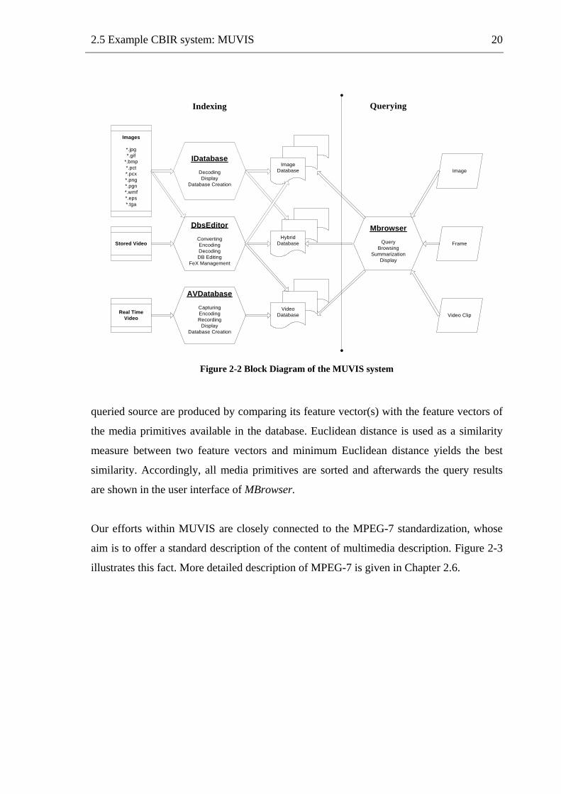
The proposed MUVIS system, which is shown in Figure 2-2, is based upon several
objectives and ideas. First of all it is intended to support real time video indexing (with or
without audio), and therefore, it has AVDatabase application specially designed for
creating audio/video databases. Corresponding application for images, IDatabase, is
developed to handle all image indexing capabilities. Second, the system is further intended
to index existing video clips regardless of their formats. DbsEditor is the application for
appending such existing video clips into an existing database. Features such as color,
texture and, shape are extracted off-line by DbsEditor. Moreover, DbsEditor can also add
and remove features to/from any type of database since MUVIS system is now being
improved to support querying based on multiple features. Finally, there is an application
called MBrowser, which is the main media retrieval and browser terminal. It has a built-in
search and query engine, which is capable of finding media primitives in any database and
for any media type that is similar with the queried media source. Retrieval results for the
2.5 Example CBIR system: MUVIS
20
IDatabaseDecodingDisplay
Database Creation
MbrowserQuery
BrowsingSummarization
Display
DbsEditorConvertingEncodingDecodingDB Editing
FeX Management
AVDatabaseCapturingEncodingRecording
DisplayDatabase Creation
Images
*.jpg*.gif
*.bmp*.pct*.pcx*.png*.pgn*.wmf*.eps*.tga
Real TimeVideo
Stored Video
ImageDatabase
VideoDatabase
HybridDatabase
Image
Frame
Video Clip
Indexing Querying
Figure 2-2 Block Diagram of the MUVIS system
queried source are produced by comparing its feature vector(s) with the feature vectors of
the media primitives available in the database. Euclidean distance is used as a similarity
measure between two feature vectors and minimum Euclidean distance yields the best
similarity. Accordingly, all media primitives are sorted and afterwards the query results
are shown in the user interface of MBrowser.
Our efforts within MUVIS are closely connected to the MPEG-7 standardization, whose
aim is to offer a standard description of the content of multimedia description. Figure 2-3
illustrates this fact. More detailed description of MPEG-7 is given in Chapter 2.6.

2.5 Example CBIR system: MUVIS
21
Figure 2-3 The role of MPEG-7 in MUVI
2.6 MPEG-7
MPEG-7 is an ISO/IEC standard developed by MPEG (Moving Picture Experts
Group)[17], formally named as “Multimedia Content Description Interface” which aims to
create a standard for describing content of multimedia data. The rapid increase in audio-
visual information has created a demand for representation that goes beyond the simple
waveform or sample-based, compression-based (such as MPEG-1 and MPEG-2) or even
object-based (such as MPEG-4) representations. MPEG-7 focuses on the interpretation of
meaning and content of information. Therefore, MPEG-7 has a key role in content-based
retrieval. In this chapter different steps of multimedia description are described. In
addition, since this thesis concentrates on shape and texture retrieval, short introduction to
these descriptors is provided. For more detailed description of these and other descriptors
in MPEG-7 the reader is referred to [10, 17, 26].
2.6.1 Overview of MPEG-7
The goal of the MPEG-7 standard is to allow interoperable searching, indexing, filtering
and access of AV content by enabling interoperability among devices and applications that
deal with AV content description. MPEG-7 describes specific features of AV content as
well as information related to AV content management. A set of methods and tools for the

2.6 MPEG-7
22
different steps of multimedia description, are described below and also presented in Figure
2-4:
• Descriptors (D) to define the syntax and the semantics of each feature.
• Description Schemes (DS) to specify the structure and semantics of the
relationships between their components that may be both Ds and DSs.
• Description Definition Language (DDL) to specify description schemes (and
possibly descriptors) to ensure extensibility of the standard.
Figure 2-4 Main elements of MPEG-7
2.6.2 Shape features
Shape information can be 2D or 3D in nature, depending on the application. The three
shape descriptors adopted by MPEG-7 are: Region Shape, Contour Shape and Shape 3D.
2D shape descriptors, the Region Shape and Contour Shape descriptors are intended for
shape matching. They do not provide enough information to reconstruct the shape nor to
define its position in an image. These two shape descriptors have been defined because of
the two major interpretations of shape similarity, which are contour-based and region-
based. Region Shape and Contour Shape descriptors as well as the Shape 3D descriptor
are described in more detail below.

2.6 MPEG-7
23
Region Shape
The shape of an object may consist of a single region or a set of regions as well as some
holes in the object. Since the Region Shape descriptor, based on the moment invariants
[26], makes use of all pixels constituting the shape within a frame, it can describe any
shape. The shape considered does not have to be a simple shape with a single connected
region, but it can also be a complex shape consisting of holes in the object or several
disjoint regions. The advantages of the Region Shape descriptor are that in addition to its
ability to describe diverse shapes efficiently it is also robust to minor deformations along
the boundary of the object. The descriptor is also characterized by its small size, fast
extraction time and matching. The feature extraction and matching processes are
straightforward. Since they have low order of computational complexities they are suitable
for shape tracking in the video sequences [17].
Contour Shape
The Contour Shape descriptor captures characteristics of a shape based on its contour. It
relies on the so-called Curvature Scale-Space (CSS) [15] representation, which captures
perceptually meaningful features of the shape. The descriptor essentially represents the
points of high curvature along the contour (position of the point and value of the
curvature). This representation has a number of important properties, namely, it captures
characteristic features of the shape, enabling efficient similarity-based retrieval. It is also
robust to non-rigid motion [17, 26].
Shape 3D
Due to the continuous development of multimedia technologies and virtual worlds, 3D
contents become a common feature in today’s information systems. The MPEG-7 Shape
3D descriptor is based on the shape spectrum concept. Shape spectrum is defined as the
histogram of the shape index, computed over the entire 3D surface [26]. The Shape 3D
descriptor provides an intrinsic shape description of 3D mesh models. It exploits some
local attributes of the 3D surface. The main applications targeted by this descriptor are
search, retrieval, and browsing of 3D model databases [17].

2.6 MPEG-7
24
2.6.3 Texture features
The three texture descriptors in MPEG-7 are [10]: Texture Browsing, Homogeneous
Texture, and Edge Histogram. Homogeneous Texture descriptor has emerged as an
important visual primitive for searching and browsing through large collections of similar
looking patterns. The Texture Browsing descriptor characterizes perceptual attributes such
as directionality, regularity, and coarseness of the texture. The Edge Histogram descriptor
represents the histogram of five possible types of edges. This descriptor is useful when the
underlying region is not homogeneous in nature. Each of these three texture descriptors is
described in more detail below.
Homogenous Texture Description
The Homogeneous Texture descriptor (HTD) [10, 17] provides a quantitative
representation that is useful for similarity retrieval. The feature extraction is done as
follows. Image is first filtered with a bank of orientation and scale turned filters (modeled
using Gabor functions). The first and second moments of energy in the frequency bands
are then used as the components of the descriptor. The number of filters used is 5x6=30
where 5 is the number of scales and 6 is the number of orientations used in the multi-
resolution decomposition using Gabor functions. The HTD feature vector is then given by:
[ 30213021, ,...,,,,...,,, dddeeeffTD SDDC= ] (2.3)
The first two components are the mean intensity and the standard deviation of the image
texture. The first and second moments of energy are denoted by ei and di.
Texture Browsing
The Texture Browsing descriptor is useful for representing homogeneous texture for
browsing type of applications. It provides a perceptual characterization of texture, similar
to human characterization, in terms of regularity, coarseness, and directionality. The
computation of this descriptor proceeds similarly as the HTD. The image is filtered using
a bank of scale and orientation selective band-bass filters and the filtered outputs are then
used to compute the texture browsing descriptor components, regularity, coarseness, and
directionality. In similarity retrieval, the Texture Browsing descriptor can be used to find a

2.6 MPEG-7
25
set of candidates with similar perceptual properties and then use the HTD to get a precise
similarity match list among the candidate images [10, 17].
Edge Histogram
The Edge Histogram descriptor represents the spatial distribution of five types of edges,
namely four directional edges and one non-directional edge. The computation of this
descriptor is done in a block-wise manner [10]. Since edges play an important role for
image perception, the Edge Histogram descriptor can retrieve images with similar
semantic meaning. Thus, it primarily targets image-to-image matching, especially for
natural images with a non-uniform edge distribution. In this context, the image retrieval
accuracy can be significantly improved if the Edge Histogram descriptor is combined with
other descriptors such as color histogram [17].

3 Human Visual Perception
Human visual perception is an important concept in the development of image retrieval
applications. Since the goal of most CBIR systems is to retrieve similar images for a given
query image corresponding to human visual system, visual perception should be taken into
consideration when selecting features and similarity measures. The detailed review of
theories of visual perception is outside the scope of this thesis. However, some of the most
important aspects related to shape and texture perception are shortly described in this
section. First we recall the useful property of human visual system, namely the lateral
inhibition. Then we consider how human visual system observes texture. Finally we relate
human similarity judgement and the similarity models used in CBIR systems.
3.1 Anatomy of the human eye
To understand the way humans perceive images, one needs to know the basics about the
anatomy of the eye, optics and the initial neural signals of the eye. Figure 3-1 shows the
main parts of a human eye. When light comes to an eye it first passes through the cornea,
then the lens, followed by the vitreous, and finally reaches the retina. The retina contains
millions of photoreceptors that capture light rays and convert them into electrical
impulses. These impulses travel along the optic nerve to the brain where they are turned
into images. At the processing step each photoreceptor on the retina generates a signal
related to the intensity of light coming from a corresponding point of the observed object.
Photoreceptors corresponding to brighter arrays of the object receive more light and
generate larger signals than those corresponding to darker areas.
26

3.1 Anatomy of the human eye
27
Figure 3-1 Anatomy of the Human Eye
3.2 Lateral Inhibition
Signals resulting from light falling on the photoreceptors are not sent directly to the brain
in the optic nerve but are instead first processed in several ways by a variety of
interactions among neurons within the retina, of which the lateral inhibition network is an
instance. Figure 3-2 gives a simplified description of the lateral inhibition network, since
humans have three layers of neurons in the retina, rather than the two shown in Figure 3-2,
but the functional outcome is the same.
Figure 3-2 The Lateral Inhibition Network
The lateral inhibition network can be characterized by a high-pass filter, which enhances
edges and intensity transitions. The schematic in Figure 3-2 illustrates a small portion of
the retina, one of those at which the overlying light pattern changes from darker to lighter,
as shown at the top of the figure. The rectangles represent photoreceptors, each generating
3.2 Lateral Inhibition
28
a signal appropriate for the amount of light falling on it. The circles represent the output
neurons of the retina, whose signals will go to the brain through the optic nerve. Each
output neuron is shown as receiving excitatory input from an overlying photoreceptor
(vertical lines) as well as inhibitory input from adjacent photoreceptors (angled lines). It is
this laterally spread inhibition that gives “lateral inhibition” networks their name. At the
bottom of the schematic is a representation of the signals in the output neurons. Output
neurons well to the right of dark/light border are excited by an overlying photoreceptor but
also inhibited by adjacent, similarly illuminated photoreceptors. The same is true far to the
left of dark/light border. Hence, assuming that the network is organized so that equal
illumination of exciting and inhibiting photoreceptors balances out, output neurons far
from the edge in either direction will have the same output signals. Only output neurons
near the dark/light border will have different output signals. As one approaches the
dark/light border from the left, the signals will decrease, because inhibition from more
brightly lit photoreceptors to the right will outweigh the excitation from the overlying
dimly lit photoreceptors. When approaching to the other direction, the signals will increase
because excitation from brightly lit photoreceptors is not completely offset by inhibition
from the dimly lit photoreceptors to the left [18].
3.3 Perception of Shape
3.3.1 Classical theories of shape perception
In [42] several classical theories of visual perception are discussed. In this chapter we
provide a short introduction to them. First of all, the Gestalt school of psychology has
played a revolutionary role with its novel approach to visual form, by producing a list of
laws for visual forms. In all of those laws visual form is considered as a whole. As
opposed to the Gestalt school, Hebb argues that form is not perceived as a whole but
consists of parts. Therefore, learning and combining aspect of perception has a key role in
Hebb’s theory. Another theory of visual perception, developed by Gibson, is centered on
perceiving real 3D objects, not their 2D projections. However, due to the non-
computational nature of these classical approaches, they are not very useful in practical
engineering approaches.
3.3 Perception of Shape
29
3.3.2 Modern theories of shape perception
In most modern theories of shape perception authors agree on the significance of high
curvature points (HCP) for visual perception [42]. The techniques used to extract those
points of interest can be roughly classified into two major categories: the ones that
perform HCP’s extraction at one scale and those that make use of different scales.
However, techniques using only one level of resolution might have several disadvantages.
In addition to finding many unimportant details, those techniques might also miss large
rounded corners. Furthermore, multi-resolution techniques do not only avoid these
problems, but also provide additional information about the “structural” importance of the
high curvature points [31].
According to [14] it is shown in several papers that the human visual system focuses on
edges and ignores uniform regions. This capability is hardwired into the retina, where two
layers of neurons perform an operation similar to Laplacian. This operation is called
lateral inhibition [see Chapter 3.2] and it helps us to extract boundaries and edges.
3.4 Perception of Texture
Texture perception, which is an important part of human visual perception, can be roughly
divided into two main approaches: feature approach and frequency approach [7]. In the
rest of this chapter both of those approaches are shortly presented.
3.4.1 Feature approach
Visual perception operates in two modes, attentive and preattentive. The preattentive
mode is a parallel, instantaneous process for extraction of features. It is independent of the
number of features and covers a large visual field. The attentive mode is a serial process,
which integrates initially separable features into unitary objects. The search area in the
attentive mode is limited to a small aperture as in form recognition. Here features mean
textons, which can be for example rectangles, ellipses or line segments with specific
colors, angular orientations, widths and lengths. According to texton theory, the
preattentive vision directs attentive vision to the locations where differences in the density
of textons occur, but ignores the positional relationships between textons [7].

3.4 Perception of Texture
30
3.4.2 Frequency approach
The human visual cortex has separate cells that respond to different frequencies and
orientations. The Gabor filter bank is a commonly applied method of texture
representation, since being able to localize the energy simultaneously both in spatial and
frequency domains Gabor functions model well the visual cortex [44]. Therefore, Gabor
decomposition is also adopted into MPEG-7 [see Chapter 2.6] where it is used both in
Homogeneous Texture Descriptor and Texture Browsing Descriptor. The latter descriptor
makes also use of two of those features Tamura et al. [16] showed to be perceptually
significant.
4 Shape Analysis
This chapter provides introduction to shape and presents three types of shape attributes:
region-based, boundary-based and multi-resolution methods. At the end of this chapter,
we introduce a novel boundary based approach to shape similarity estimation based on
distance transformation and ordinal correlation. Experiments using this algorithm for
shape-based image retrieval are also provided.
4.1 Introduction to Shape
The shape of an object is a binary image representing the extent of objects. Shape
representations techniques used in similarity retrieval are generally characterized as being
region-based and boundary-based. The former considers the shape being composed of a
set of two-dimensional regions, while the latter presents the shape by its outline. Region-
based feature vectors often result in shorter feature vectors and simpler matching
algorithms. However, generally they fail to produce efficient similarity retrieval. On the
other hand, feature vectors extracted from boundary-based representations provide a richer
description of the shape. This scheme has led to the development of the multi-resolution
shape presentations, which proved very useful in similarity assessment [31]. The idea in
multi-resolution techniques is to decompose a planar curve contour into components at
different scales so that the coarsest scale components carry the global approximation
information while the finer scale components contain the local detail information.
31
4.2 Shape Attributes
32
4.2 Shape Attributes
4.2.1 Region-based attributes
Simple geometric attributes
Description of the geometric properties of a region can be obtained measuring properties
of points belonging to the region. Those properties are for example [3, 31]:
• area : can be measured as the count of internal pixels.
• bounding rectangle : is the minimum rectangle enclosing the object.
• aspect ratio: is invariant to the scale of the object, since it is computed as the radio
of the width and length of the rectangle.
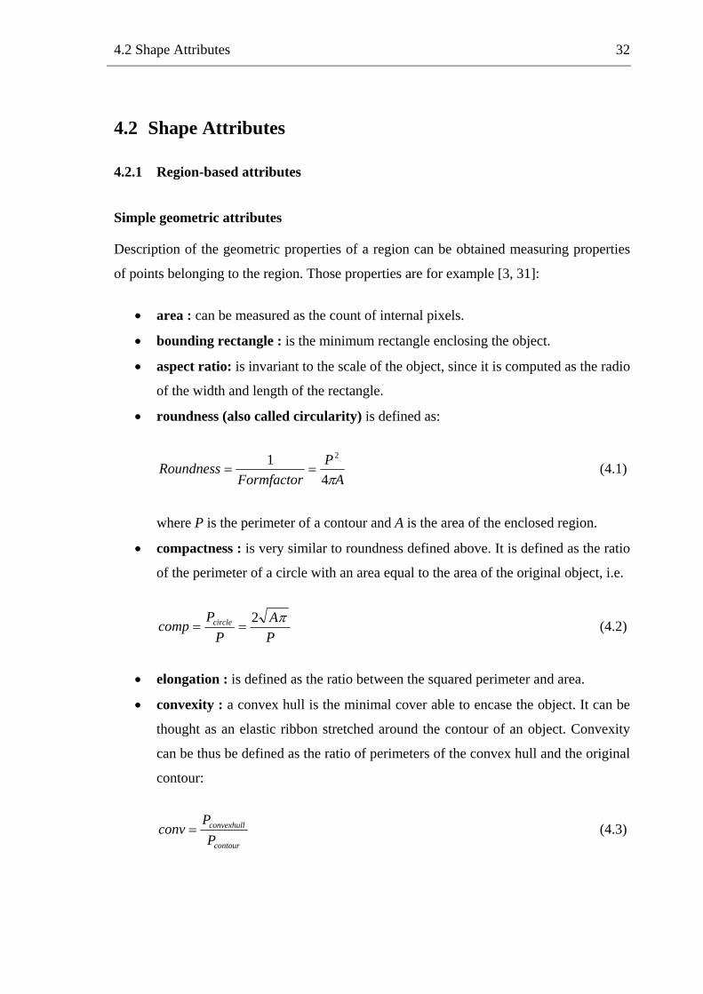
• roundness (also called circularity) is defined as:
AP
FormfactorRoundness
π41 2
== (4.1)
where P is the perimeter of a contour and A is the area of the enclosed region.
• compactness : is very similar to roundness defined above. It is defined as the ratio
of the perimeter of a circle with an area equal to the area of the original object, i.e.
PA
PP
comp circle π2== (4.2)
• elongation : is defined as the ratio between the squared perimeter and area.
• convexity : a convex hull is the minimal cover able to encase the object. It can be
thought as an elastic ribbon stretched around the contour of an object. Convexity
can be thus be defined as the ratio of perimeters of the convex hull and the original
contour:
contour
convexhull
PP
conv = (4.3)

4.2 Shape Attributes
33
• ratio of principal axes : principal axes are defined uniquely as the segments of
lines crossing each other orthogonally in the centroid of the object representing the
directions with zero correlation. The lengths of the principal axes are equal to the
eigenvalues λ1,2 of the covariance matrix C [31].
• circular variance : describes how close a shape is to a circle. The proportional
mean square error with respect to a solid circle or circular variance is defined as:
( )∑ −−=i
rir
pN
c 22
1var µµµ
(4.4)
where ∑ −==
i ir pN µµ /1 is the mean radius, pi = (xi, yi) is the ith contour
point, µ is the centroid of the region and N is the number of contour points.
• elliptic variance : is an extension to the circular variance measure, which allows
the elongation of the shape, i.e. fitting an ellipse that has an equal covariance
matrix C and measuring the mapping error evar:
( ) ( )( )∑ −−−= −
ircii
rc
ppN
e2
1'1var µµµµ
C (4.5)
, where ( ) ( )∑ −−= −i iirc ppN µµµ 1'/1 C .
The simple geometric attributes are widely used in image retrieval. Simple descriptors,
such as area and eccentricity, with (weighted) Euclidean distance function are used in
QBIQ [12]. Simple geometric descriptors are robust to noise and mostly also robust to
scale, rotation, and orientation. Moreover, these shape attributes are often very easily
calculated and result in short feature vectors. However, these descriptors are not stable,
since perceptually insignificant variations in the shapes may result in significant variations
in some of the descriptors [31].
Invariant moments
For a 2D continuous function f(x,y), the moment of order (p+q) can be defined as [36]:
∫ ∫∞
∞−
∞
∞−
= dxdyyxfyxm qppq ),( (4.6)

4.2 Shape Attributes
34
Moments mpq are uniquely defined by the shape function f(x,y), and the moments mpq are
sufficient to reconstruct the original region function f(x,y). In other words, moment-based
shape description is information preserving. The central moments are defined as:
∫ ∫∞
∞−
∞
∞−
−−= dxdyyxfyyxxM qc
pcpq ),()()( (4.7)
where xc=M10(R)/M00(R) and yc=M01(R)/M00(R) define the center of mass (centroid) and R is
the region of interest.
If f(x,y) is a digital image, then Mpq becomes
( ) ( )∑∑ −−=
x
qc
p
ycpq yxfyyxxM ),( (4.8)
It is important for shape descriptors to be invariant to scaling, translation, and rotation.
Therefore, a normalized definition of moments ηnq is needed.
( ) ...,3,212/,00
=+++== qpforqpwhereMM pq
pq γη γ (4.9)
A set of seven invariant moments can be derived from the second and third order
normalized moments [36]:
02201 ηηφ += (4.10)
211
202202 4)( ηηηφ ++= (4.11)
20321
212303 )3()3( ηηηηφ −+−= (4.12)
20321
212304 )()( ηηηηφ +++= (4.13)
[ ][ ]2
03212
123003210321
20321
21230123012305
)()(3))(3(
)(3)())(3(
ηηηηηηηη
ηηηηηηηηφ
+−++−
++−++−= (4.14)
[ ] ))((4)()()( 03211230112
03212
123002206 ηηηηηηηηηηηφ ++++−++= (4.15)

4.2 Shape Attributes
35
[ ][ 2
03212
123003213012
20321
21230123003217
)()(3))(3(
)(3)())(3(
ηηηηηηηη
ηηηηηηηηφ
+−++−
++−++−=
] (4.16)
These moments are invariant to translation, rotation, and scale change [36]. Another major
advantage of this method is that the images do not need to be segmented in order to obtain
the shape description of images. The invariant moments can be obtained by integrating
directly over the actual intensity values of the image (f(x,y)) [31]. Because of these
attractive properties invariant moments have been used in some CBIR system such as the
QBIC system [12]. However, this approach fails to provide enough information to account
for inter-class variations.
4.2.2 Boundary-based attributes
This chapter introduces shortly three boundary-based representations of an object.
Typically boundary-based representations include two major steps. First, a 1D function is
constructed from a 2D shape boundary parametrizing the contour. Then the constructed
1D function is used to extract a feature vector describing the shape of the object.
Chain code
Chain codes are used to represent a boundary by a connected sequence of straight-line
segments of specified length and direction. Usually this representation is based on 4- or 8-
connectivity of the segments. Some examples of chain codes can be found in [36].
Producing the chain code using all the pixel pairs in the image would lead to two major
disadvantages. First the resulting chain code would be long, and secondly any disturbances
along the boundary could cause changes in the code. Therefore, a common approach to
avoid these problems is to resample the boundary by selecting a larger grid spacing.
The chain code of a boundary depends on the starting point. However, the code can be
normalized easily using the following procedure. The chain code is treaded as a circular
sequence of direction numbers and the starting point is redefined so that the resulting
sequence forms an integer of minimum magnitude. However, the normalization is exact
only if the boundary is invariant to rotation and scale change [36].

4.2 Shape Attributes
36
Fourier Descriptors (FD)
The boundary of an object can be represented as the sequence of the coordinates
u(k)=[x(k), y(k)], for k = 0, 1, 2, … , K-1. Moreover, each coordinate pair can be treated as
a complex number so that
( ) ( ) ( ).kjykxku += (4.17)
The Discrete Fourier Transform (DFT) of u(k) and its inverse is given as in [31]:
( ) ( ) ( ) ( ) 10,2exp1
0
−≤≤=⎥⎦⎤
⎢⎣⎡−= ∑
−
=
KnenMK
nkjkunFK
k
kfθπ (4.18)
( ) ( ) 10,2exp1 1
0−≤≤⎥⎦
⎤⎢⎣⎡= ∑
−
=
KnK
nkjnFK
kuK
n
π (4.19)
where K is the number of boundary samples and M(n) is the magnitude of the Fourier
Descriptors.
The complex coefficients F(n) are called the Fourier Descriptors (FD) of the boundary.
Let’s suppose, however, that instead of all the F(n)’s, only the first M coefficients are
used. This leads to the following approximation:
( ) ( )∑−
=
−≤≤⎥⎦⎤
⎢⎣⎡=
1
010,2expˆ
M
uKk
KnkjnFku π (4.20)
Although only M terms are used to obtain each component of û(k), k still ranges from 0 to
K-1. This means that same amount of points exists in the approximate contour, but fewer
points are needed in the reconstruction of each point. Due to the fact that high frequency
components account for finer details and low frequency components determine global
shape, the smaller M becomes, the more details are lost on the contour.
The major advantage of FD is that it is easy to implement. In addition, it is also robust to
noise and invariant to geometric transformations. However, according to [31] Fourier
Descriptor method performs rather poorly on similarity retrieval. Reason for this might be

4.2 Shape Attributes
37
that the frequency terms have no obvious counter-part in human vision. Another difficulty
with the FD is that the used basis functions are global sinusoids, which fail to provide a
special localization of the coefficients. Therefore, problems occur when performing query
using occluded images [31].
Polygonal Approximation
As mentioned in Chapter 3.3.2, human visual system decomposes objects using points of
high negative curvature. Therefore, approximating curves by straight lines joining these
high curvature points (HCP) preserve enough information necessary for successful shape
recognition. Thus the polygonal approximation of contours at high curvature points
compresses effectively the shape information in a sequence of few vertices [31]. As can be
seen in Chapter 4.2.3 polygonal approximation can be utilized in a shape recognition
technique base on Wavelet-Transform Modulus Maxima.
4.2.3 Multi-resolution attributes
This chapter utilizes contour representations based on multi-resolution decomposition.
Multi-resolution techniques have several advantages: they neglect unimportant details, but
provide also additional information about the “structural” importance of high curvature
points [31]. We present here two methods using this approach. First is the CSS technique,
which is based on the scale space smoothing of the curvature function. Second, the
wavelet transform, which decomposes the orientation profile of the contour, was utilized
to extract high curvature points at multiple scales. Both of these techniques are presented
in more detail below.
The Curvature Scale Space (CSS)
A CSS is a multi-scale organization of the inflection points (or curvature zero-crossing
points) of the contour as it evolves. Intuitively, curvature is a local measure of how fast a
planar contour is turning. Therefore, it can be defined as the derivative of the tangent
angle to the curve. If we consider a parametrized contour:
( ) ( ) ( )( ) [ ]{ 1,0, ∈=Γ uuyuxu } (4.21)
where u is the normalized arc length parameter.

4.2 Shape Attributes
38
The formula for computing the curvature function (for any parametrized curve) can be
expressed as [31]:
( ) ( ) ( ) ( ) ( )( ) ( )( ) 2/322 uyux
uyuxuyuxu+−
=κ (4.22)
The heart of the CSS technique is based on curve evolution, which basically studies the
shape properties while deforming in time. The evolution process can be achieved by
Gaussian smoothing and computing the curvature at various levels of detail. Let g(u,σ) be
a 1D Gaussian kernel of width σ :
( ) ⎟⎟⎠
⎞⎜⎜⎝
⎛−= 2
2
2exp
21,
σσπσ uug (4.23)
where σ is also referred to as scale parameter. Let X(u,σ) and Y(u,σ) represent the components of the evolved curve:
( ) ( ) ( )σσ ,, uguxuX ∗= ( ) ( ) ( )σσ ,, uguyuY ∗= (4.24)
where (*) is the convolution operation. The derivative for each component can be
calculated easily:
( ) ( ) ( )σσ ,, uguxuX uu ∗= ( ) ( ) ( )σσ ,, uguxuX uuuu ∗= (4.25)
where gu(u,σ) and guu(u,σ) are the first and second derivative of the Gaussian filter,
respectively. The same formulas apply for computing Yu(u,σ) and Yuu(u,σ). Using the
above equations the curvature of an evolved curve contour can be computed using the
following formula:
( ) ( ) ( ) ( ) ( )( ) ( )( ) 2/322 ,,
,,,,,
σσσσσσ
σκuYuX
uYuXuYuXu
uu
uuuuuu
+
−= (4.26)
Now the function defined implicitly by κ(u,σ)=0 is the CSS image of Γ. This is a two
dimensional map of the inflection points or zero curvature points detected at different
scales. In practice, to obtain the CSS image, the smoothing process is started with σ=1,
which is increased at each level until a convex contour is obtained. The CSS image is then

4.2 Shape Attributes
39
the plot of these points in the (u,σ) plane. The corresponding feature vector summarizes
the CSS image into just few maxima of significant lobes in the CSS image. If (ui,,σi) are
the maxima points of the significant lobes, then the shape feature vector is given by:
( ) ( ) ({ NNii uuu ) }σσσ ,...,,...,, 11 (4.27)
This CSS technique is used for example in SQUID system and when compared against
moments and Fourier descriptors, it outperformed both of them. The CSS technique is also
adopted as MPEG-7 Contour Shape descriptor [26].
Wavelet Transform Modulus Maxima (WTMM)
Many authors agree on the significance of high curvature points (HCP) for visual
perception [42]. Since, in CSS technique planar curves smoothed using Gaussian kernel
suffer from shrinkage [31], the tracking and correct localization of high curvature points
becomes more difficult. However, the wavelet decomposition avoids this problem due to
the spatial and frequency localization property of wavelet spaces, and is therefore a very
useful method for detecting local features of a curve [31].
Since biquadratic wavelets perform better than other wavelets for corner detection
applications [43], their usage is introduced here. First, the boundary is tracked and the
orientation profile is calculated as in [24]. To obtain the same number of points for each
contour, the orientation profile for each shape is sampled and interpolated. The Wavelet
transform of the orientation profile is calculated for dyadic scales from 21 to 26. For the
purpose of extracting few important high curvature points useful for polygonal
approximation, we select the WTMM maxima above a certain threshold in each level at
scale s = 2j (j = 1,2, ...,6), track them down to lower scales and determine the exact
location of these HCP on the contour. The feature vector of the given shape will contain
the location and magnitude of the WT at each HCP. Similarity scores are then estimated at
each level of the decomposition independently. Finally, the overall similarity score is
computed as the maximum value of the single level similarity scores [13].

4.2 Shape Attributes
40
The WTMM approach is effective since the exact location of the HCP is determined with
high precision by tracking the WTMM through the decomposition levels until the original
contour. Due to the use of dyadic scales this technique is much faster than CSS, in which
the full continuous scale decomposition is required. Furthermore, since the WTMM
approach keeps most of the shape information, the object contour can be accurately
reconstructed from its WTMM [34].
4.3 Shape Correspondence using Ordinal Measures
In this chapter we introduce a novel boundary-based approach to shape similarity
estimation [14]. The proposed method operates in three steps: alignment, boundary to
multi-level transformation, and similarity evaluation. Once the boundaries are aligned, the
binary images containing the boundaries are transformed into multilevel images using a
distance transformation [35]. The transformed images are then compared using the ordinal
correlation measure introduced in [8, 21]. In this chapter we give a detailed description of
each one of the steps mentioned above.
4.3.1 Object alignment based on universal axes
The alignment of the shapes is performed by first detecting the three universal axes [22]
for each shape, then aligning each object using their axes in a standard way. The steps of
the alignment algorithm are given below.
Step 1. Translate the coordinate system so that the origin becomes the center of gravity of
the shape S.
Step 2. Compute
( ) ( ) ( )∫ ∫ ∫ ∫=⎟⎟
⎠
⎞
⎜⎜
⎝
⎛
+
++=+
S S
illll dxdyerdxdyyx
iyxyxyx θµµµµ 22
22 (4.28)
using the normalized counterpart (called Universal Axes (UA) )

4.3 Shape Correspondence using Ordinal Measures
41
( )( ) ( )
( ) .3,2,1,~~22
=+
+=+∫ ∫
lfordxdyyx
iyxyix
S
llll
µ
µµµµ (4.29)
Step 3. Compute the polar angle Θµ ∈ [0, 2π] so that
( ) ( )11 lli yxeR µµµ
µ +=Θ (4.30)
where l1 is the number of axes needed to align an object.
Step 4. Compute the directional angles of the l1 universal axes of the shape S as follows:
( ) 111
...,,2,1,21 ljforl
jlj =−+Θ
=πθ µ (4.31)
In our implementation we used l1=3, since only two axes cannot be used alone to
determine if an object is flipped around the direction they define or not.
Step 5. Once the tree universal axes are determined, rotate the contour so that the most
dominant UA (UA with the largest magnitude) will be aligned with the positive x-axis.
Step 6. Then, if the y-component of the second most dominant UA is positive, flip the
contour around the x-axis.
The performance of the alignment procedure is illustrated by applying it to the set of
contours shown in Figure 4-1. The results of the alignment are presented in Figure 4-2. It
can be noticed that this alignment scheme is able to solve both problems of rotation and
mirroring.

4.3 Shape Correspondence using Ordinal Measures
42
Figure 4-1 Bird contours from the MPEG-7 shape test set B
Figure 4-2 The birds contours after alignment
4.3.2 Boundary to multilevel image transformation
Let shape S be represented by its contour C in a binary image. The binary image is
transformed into a multilevel image G using a mapping function φ, such that the pixel
values in G, {G1, G2,…, Gn}, depend on their relative position to the contour pixels C1, C2,
…, Cp:

4.3 Shape Correspondence using Ordinal Measures
43
( ) niforpkCG ki ...,,2,1,...,,2,1: === φ (4.32)
where Ck is the position of the contour pixel k in the image G.
Resulting form this mapping the shape boundary information will be spread throughout all
the pixels of the image. An example of the distance map can be seen in Figure 4-3.
Computing the similarity in the transform domain will benefit from the rearrangement of
the boundary information in the new image. We assume that no single optimal mapping
exists: different mappings will emphasize different features of the contour.
In this work we implemented the distance mapping based on the geodesic distance. The
metric is integer and the mapping is done using an iterative wave propagation process
[20]. The contour points are considered as seeds during the construction of the distance
map. The distance map can be generated inside and/or outside the contour. The values can
increase or decrease starting from the contour and can be limited. Therefore, the pixel
values in the distance map can be written as follows:
,...,,2,1,),(0 niforCPdVG ii =±= (4.33)
where V0 is the value on the contour and d(Pi , C) is the distance from any point Pi in the
image contour C.
Figure 4-3 The distance map generated for the "bird-01"

4.3 Shape Correspondence using Ordinal Measures
44
4.3.3 Similarity evaluation
The image similarity evaluation is based on the framework for ordinal-based image
correspondence introduced in [21]. Figure 4-4 gives a general overview of this region-
based approach.
Suppose we have two equal sized images, X and Y. In a practical setting images are resized
into a common size. Let {X1, X2, …, Xn} and {Y1, Y2, …,Yn} be the pixels of images X and
Y, respectively. We select a number of areas {R1, R2, …, Rn}and extract from both images
the pixels belonging to these areas. Let RjX and Rj
Y be the pixels from images X and Y,
which belong to areas Rj, with j = 1, 2, …, m.
Figure 4-4 The general framework for ordinal correlation of images
The idea is to compare the two images using a region-based approach. To achieve this, we
will be comparing RjX and Rj
Y for each j = 1, 2, …, m. Thus, each block in image X is
compared to the corresponding block in image Y in an ordinal fashion. The ordinal
comparison of the two regions means that only the ranks of the pixels are utilized. For
every pixel Xk, we construct a so-called slice SkX = { Sk,l:l = 1, 2, …,n }, where

4.3 Shape Correspondence using Ordinal Measures
45
⎩⎨⎧ <
=otherwise
XXifS lkX
lk ,0,1
, (4.34)
As can be seen, slice Sk
X corresponds to pixel Xk and is a binary image of size equal to
image X. Slices are built similarly for image Y as well.
To compare the regions RjX and Rj
Y, we first combine the slices from image X,
corresponding to all the pixels belonging to region RjX. The slices are combined into a so-
called metaslice MjX using the operation OP1(.), which is chosen to be a component-wise
summation operation. Therefore, metaslice MjX is the summation of all slides
corresponding to the pixels in block j in image X. More formally this can be written:
{ }( ) ∑
∈
==∈=jk RXk
kXjk
Xk
Xj mjforSRXSOPM
:1 ....,,2,1,: (4.35)
Similarly, we combine the slices from image Y to form Mj
Y for j = 1, 2, …, m. It should be
noted that the metaslices are equal in size to the original images and could be multivalued,
depending on the operation OP1(.). Each metaslice represents the relation between the
region it corresponds to and the entire image.
The following step is a comparison between all pairs of metaslices MjX and Mj
X using the
operation OP2, which is chosen to be the squared Euclidean distance. This results in the
metadifference Dj, which is defined as:
( ) ....,,2,1,,2
22 mjforMMMMOPD Yj
Xj
Yj
Xjj =−== (4.36)
Then we construct a set of metadifferences D = {D1, D2, …, Dm}. The final step is to
extract a scalar measure of correspondence from set D, using operation OP3(.), which sums
together all metadifferences. In other words,
....,,2,1,)(3 mjforDDOP
jj === ∑λ (4.37)
Small values of λ mean similar objects. As it was shown in [21], this structure could be
used to model the well-known Kendall’s τ and Spearman’s ρ measures.
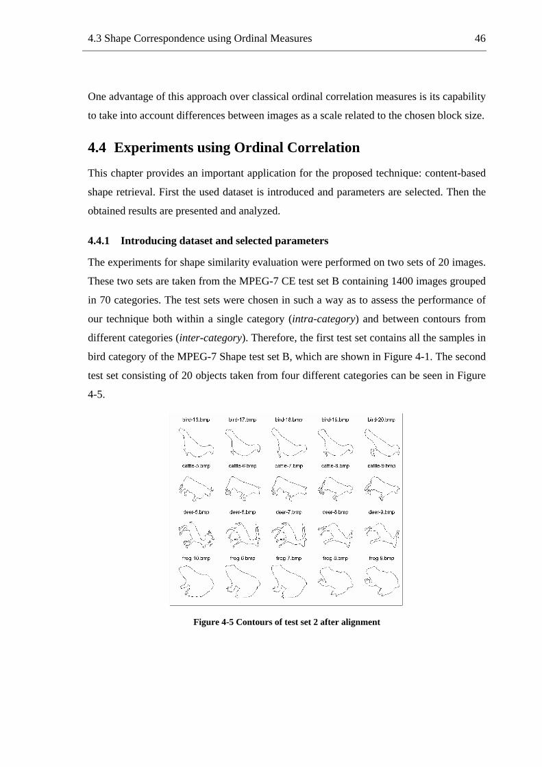
4.3 Shape Correspondence using Ordinal Measures
46
One advantage of this approach over classical ordinal correlation measures is its capability
to take into account differences between images as a scale related to the chosen block size.
4.4 Experiments using Ordinal Correlation
This chapter provides an important application for the proposed technique: content-based
shape retrieval. First the used dataset is introduced and parameters are selected. Then the
obtained results are presented and analyzed.
4.4.1 Introducing dataset and selected parameters
The experiments for shape similarity evaluation were performed on two sets of 20 images.
These two sets are taken from the MPEG-7 CE test set B containing 1400 images grouped
in 70 categories. The test sets were chosen in such a way as to assess the performance of
our technique both within a single category (intra-category) and between contours from
different categories (inter-category). Therefore, the first test set contains all the samples in
bird category of the MPEG-7 Shape test set B, which are shown in Figure 4-1. The second
test set consisting of 20 objects taken from four different categories can be seen in Figure
4-5.
Figure 4-5 Contours of test set 2 after alignment

4.4 Experiments using Ordinal Correlation
47
In both experiments, the similarity score λ is computed for all the pairs of shapes in the
set. The distance maps were generated inside the objects with V0 = 50, since this setting
emphasizes the skeleton and gives less importance to the contour pixels. The transformed
images are resized to 32x32 pixels and blocks of size 4x4 were used. If more precision is
needed, large images can be used, but this implies creation of more slides, and therefore,
the need for computational power increases.
4.4.2 Results and their evaluation
Figure 4-6 presents a surface plot of the similarity scores for the test set 1. It shows that
within the same category, the scores have small values, meaning that the corresponding
images are quite similar according to our measure. It is also worth noticing that the scores
on the diagonal are zero meaning that each object is identical to itself, so there is no bias
in the similarity scores. Blue, especially dark blue, regions in Figure 4-6 represent very
low scores (close to zero), which shows that there are quite many objects in this category
which are very similar or even identical.
To find out most similar contours to a given contour in Figure 4-5 we sort the scores
corresponding to this contour. From Figure 4-6 and Figure 4-7 one can easily estimate
which are the most similar objects for each object, based on the clustered dark blue cells.
Figure 4-7 shows that similarity scores between subjects from the same category are low,
while those obtained from subjects from different categories are relatively high. Therefore,
sorting the scores in ascending order will yield the most similar objects first.
Generally, the inter-category scores obtained by our similarity estimation technique are
larger than the intra-category ones. Thus, this technique can be used in shape
classification. Moreover, due to its sensitivity to intra-category variations it can be used in
content-based retrieval system. In addition, the developed technique can also be used in
objective performance evaluation of segmentation algorithms [1, 14, 27].

4.4 Experiments using Ordinal Correlation
48
Figure 4-6 The similarity scores for the test set 1
Figure 4-7 The similarity scores for the test set 2

5 Texture Analysis
This chapter provides first an introduction to texture. Following three different types of
texture attributes are presented: spatial, frequency, and moment-based attributes. At the
end of the chapter an application for rock texture retrieval using gray level co-occurrence
matrix is provided. Results obtained are also compared to those of Gabor wavelet features.
5.1 Introduction to Texture
Although no formal definition to texture exists, there are several of intuitive properties of
texture, which are generally assumed to be true [33]. Texture is a property of area, and
therefore, its definition must involve gray values in a spatial neighborhood. The size of the
neighborhood depends on the texture type, or the size of the primitives defining the
texture. Texture involves also the spatial distribution of gray levels and therefore two-
dimensional histograms or co-occurrence matrices are reasonable texture analysis tools.
There are several properties, such as coarseness, contrast, and directionality, which play an
important role in describing texture. Coarseness measures texture scale (average size of
regions that have the same intensity), contrast measure vividness of the texture (depends
on the variance of the gray-level histogram), and directionality gives the eventual main
direction of the image texture. Formulas to calculate these attributes can be found in [3].
Texture analysis is important, since texture is useful in various applications such as
automated inspection, medical image processing, remote sensing, defect detection and,
similarity evaluation.
49

5.2 Texture Attributes
50
5.2 Texture Attributes
5.2.1 Spatial Methods
Co-occurrence matrix
Gray level co-occurrence matrix (GLCM), originally introduced by Haralick [38]
estimates image properties related to second-order statistics taking into account the spatial
arrangement of gray-level primitives. Each entry (i,j) in GLCM corresponds to the number
of occurrences of the pair of gray levels i and j which are a distance d apart in original
image. Well-known statistics of the co-occurrence probabilities have been used to
characterize properties of a textured region. More detailed description of the method will
be provided in Chapter 5.3.
Auto-correlation function
An important property of many textures is the repetitive nature of the placement of texture
elements. The auto-correlation function of an image can be used to assess the amount of
regularity as well as the fineness and coarseness of the texture. If the texture is coarse,
then the auto-correlation function will drop slowly with distance; otherwise it will drop
very rapidly. Formally, the autocorrelation function of an image I(x,y) is defined as
follows [33]:
∑∑
∑∑
= =
= =
++= M
u
N
v
M
u
N
v
vuI
yvxuIvuIyx
0 0
2
0 0
),(
),(),(),(ρ (5.1)
where x, y is the position difference in u, v direction, and M, N are the image dimensions.
Fractal dimension
The fractal dimension gives a measure of the roughness of a surface. First we define a
deterministic fractal in order to introduce some of the fundamental concepts. Self-
similarity across scales in fractal geometry is a crucial concept. A deterministic fractal is
defined using this concept as follows. If A is a bounded set in an Euclidean n-space, the set

5.2 Texture Attributes
51
A is said to self-similar when A is the union of N distinct copies of itself, each of which
have been scaled down by a ratio of r. The fractal dimension D is related to the number N
and the ratio of r as follows:
)/1log(log
rND = (5.2)
There are several methods proposed for estimating the fractal dimension D. In [33] two of
them are presented and here we describe the other improved version. Let us assume that
we are estimating the fractal dimension of an image A. Let P(m, L) be the probability that
there are m points within a box of side length L centered at an arbitrary point on a surface
A. Let M be the total number of points in the image. When one covers the image with
boxes of side length L, then the (M/m)P(m,L) is the expected number of boxes with m
points inside. The expected number of boxes needed to cover the whole image is
( )[ ] ( ) (∑=
=N
mLmPmMLNE
1,/1 ) (5.3)
The expected value of N(L) is proportional to L-D and thus it can be used to estimate the
fractal dimension D. However, the fractal dimension itself is not sufficient to capture all
textural properties. Therefore, another measure, called lacunarity is suggested to
discriminate between fine and coarse textures having same fractal dimension [33].
5.2.2 Frequency-based methods
Power spectrum
For the frequency-based approach a good solution is to partition the image into a set of
non-overlapping nxn blocks and compute the power spectrum separately for each block.
Maxima of the spectrum can be used as parameters for modeling texture properties. Each
periodical pattern in the original spatial domain is represented by a peak in the power
spectrum. Respectively, images including non-periodical or random patterns have a power
spectrum in which peaks are not easy to detect.

5.2 Texture Attributes
52
Wavelet transform
Gabor wavelet decomposition enables simultaneous localization of energy in both spatial
and frequency domains. This localization has been shown to be optimal in the sense of
minimizing the joint two-dimensional uncertainty in space and frequency. The Gabor
representation is also an essential part of the MPEG-7 standard, where it is used in Texture
Browsing Descriptor and Homogeneous Texture Descriptor. More detailed description of
the Gabor wavelet decomposition will be given in Chapter 5.4.
5.2.3 Moment-based methods
This chapter introduces moment-based texture attributes. First the feature extraction for
textured images using moments is explained. Then two sets of orthogonal moments,
Zernike moments and Fourier-Mellon moments are described.
Texture feature extraction using moments
In the moment-based method the texture features are obtained directly from the gray-level
image f(x,y) by computing the moments of the image in local regions. The (p+q)th order
moments of a function of two variables f(x,y) with respect to the origin is defined as in
Equation 4-6. Let (i,j) be the pixel coordinates for which the moments are computed.
Given a window width W, the coordinates are normalized to the range [-1,1] and the
normalized coordinates (xm, yn) are given by:
.2/
,2/ W
jnyW
imx nm−
=−
= (5.4)
The moments within a window centered at pixel (i,j) are computed by a discrete sum
approximation which uses normalized coordinates (xm, yn) [29]:
( )∑ ∑− −
=2/
2/
2/
2/,
W
W
W
W
qn
pmm yxnmfx (5.5)
Since this discrete computation of the set of moments for a given pixel over a finite
rectangular window corresponds to a neighborhood operation, it can be interpreted as

5.2 Texture Attributes
53
convolution with a mask. Following are the masks corresponding to the moments up to
three with a window size of three.
⎥⎥⎥
⎦
⎤
⎢⎢⎢
⎣
⎡=
111111111
00m⎥⎥⎥
⎦
⎤
⎢⎢⎢
⎣
⎡
−−−
=101101101
10m⎥⎥⎥
⎦
⎤
⎢⎢⎢
⎣
⎡ −−−=
111000111
01m⎥⎥⎥
⎦
⎤
⎢⎢⎢
⎣
⎡
−
−=
101000101
11m
⎥⎥⎥
⎦
⎤
⎢⎢⎢
⎣
⎡=
111000111
02m⎥⎥⎥
⎦
⎤
⎢⎢⎢
⎣
⎡=
101101101
20m⎥⎥⎥
⎦
⎤
⎢⎢⎢
⎣
⎡
−
−=
101000101
12m⎥⎥⎥
⎦
⎤
⎢⎢⎢
⎣
⎡ −−=
101000101
21m
Before calculating the moments the scale should be selected by choosing the size of the
window. As the window size gets larger, more global features are detected. The image
with larger texture tokens would require larger window size whereas finer textures would
benefit from smaller windows.
The set of values for each moment over the entire image can be regarded as a new feature
image. However, moments alone are not sufficient to obtain good texture features in
certain images. In [29] it was suggested to use a nonlinear transducer that maps moments
to texture features. For example hyperbolic tangent function could be used for the
nonlinear transformation, which transforms the moment images Mk with mean to
corresponding texture feature images. The transformation can be written as follows:
( ) ( )( )( )( )∑∈
−=jiwba
kk MbaMN
jiF,,
,tanh1, σ (5.6)
where N is the number of pixels in the window Wi,j, (i,j) is the center of window and σ
controls the shape of the logistic function.
Zernike moments
Using Zernike basis function to replace the non-orthogonal basis function we get the
definition for the orthogonal Zernike moments of order n and repetition l [29]:
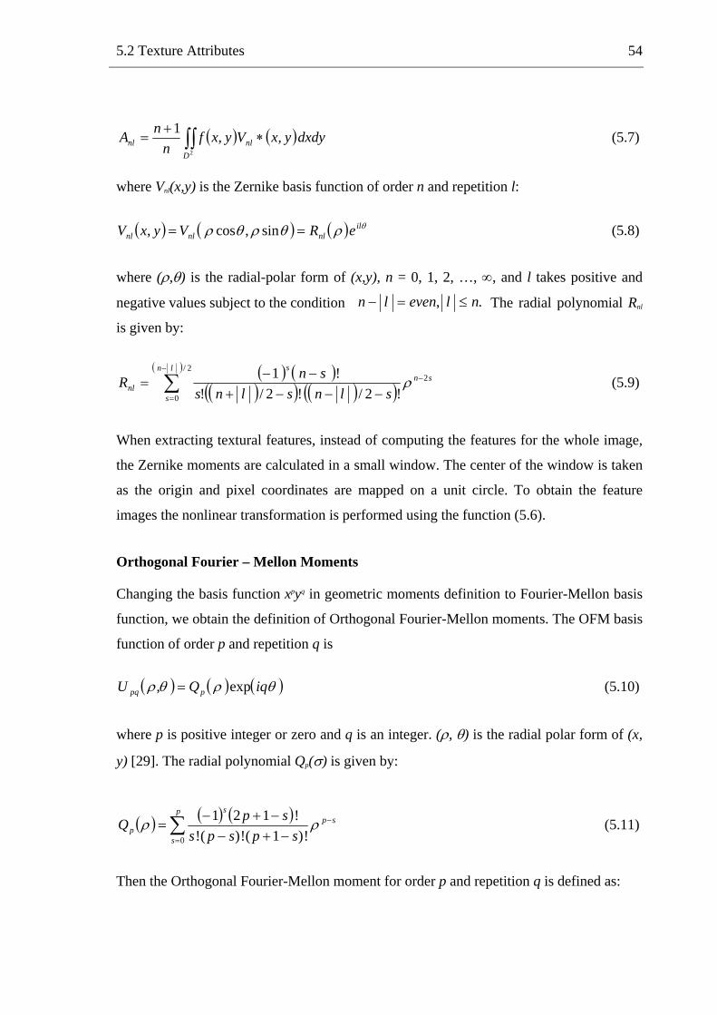
5.2 Texture Attributes
54
( ) ( )∫∫ ∗+
=2
,,1
Dnlnl dxdyyxVyxf
nnA (5.7)
where Vnl(x,y) is the Zernike basis function of order n and repetition l:
( ) ( ) ( ) θρθρθρ il
nlnlnl eRVyxV == sin,cos, (5.8)
., nlevenln ≤=−
where (ρ,θ) is the radial-polar form of (x,y), n = 0, 1, 2, …, ∞, and l takes positive and
negative values subject to the condition The radial polynomial Rnl
is given by:
( ) ( )
( )( ) ( )( )( )
∑−
=
−
−−−+−−
=2/
0
2
!2/!2/!!1ln
s
sns
nl slnslnssnR ρ (5.9)
When extracting textural features, instead of computing the features for the whole image,
the Zernike moments are calculated in a small window. The center of the window is taken
as the origin and pixel coordinates are mapped on a unit circle. To obtain the feature
images the nonlinear transformation is performed using the function (5.6).
Orthogonal Fourier – Mellon Moments
Changing the basis function xpyq in geometric moments definition to Fourier-Mellon basis
function, we obtain the definition of Orthogonal Fourier-Mellon moments. The OFM basis
function of order p and repetition q is
( ) ( ) ( )θρθρ iqQU ppq exp, = (5.10)
where p is positive integer or zero and q is an integer. (ρ, θ) is the radial polar form of (x,
y) [29]. The radial polynomial Qp(σ) is given by:
( ) ( ) ( )∑=
−
−+−−+−
=p
s
sps
p spspsspQ
0 !)1(!)(!!121 ρρ (5.11)
Then the Orthogonal Fourier-Mellon moment for order p and repetition q is defined as:
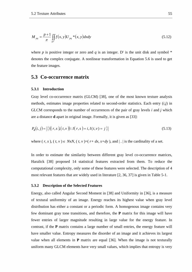
5.2 Texture Attributes
55
( ) ( )∫∫+
=2
,*,1
Dpqpq dxdyyxUyxfpM
π (5.12)
where p is positive integer or zero and q is an integer. D2 is the unit disk and symbol *
denotes the complex conjugate. A nonlinear transformation in Equation 5.6 is used to get
the feature images.
5.3 Co-occurrence matrix
5.3.1 Introduction
Gray level co-occurrence matrix (GLCM) [38], one of the most known texture analysis
methods, estimates image properties related to second-order statistics. Each entry (i,j) in
GLCM corresponds to the number of occurrences of the pair of gray levels i and j which
are a distance d apart in original image. Formally, it is given as [33]:
( ) ( ) ( )( ) ( ){ }jvtIisrIvtsrjiP === ),(,,:,,,,d (5.13)
where ( r, s ), ( t, v ) ∈ NxN, ( t, v )=( r+ dx, s+dy ), and | . | is the cardinality of a set.
In order to estimate the similarity between different gray level co-occurrence matrices,
Haralick [38] proposed 14 statistical features extracted from them. To reduce the
computational complexity, only some of these features were selected. The description of 4
most relevant features that are widely used in literature [2, 36, 37] is given in Table 5-1.
5.3.2 Description of the Selected Features
Energy, also called Angular Second Moment in [38] and Uniformity in [36], is a measure
of textural uniformity of an image. Energy reaches its highest value when gray level
distribution has either a constant or a periodic form. A homogenous image contains very
few dominant gray tone transitions, and therefore, the P matrix for this image will have
fewer entries of larger magnitude resulting in large value for the energy feature. In
contrast, if the P matrix contains a large number of small entries, the energy feature will
have smaller value. Entropy measures the disorder of an image and it achieves its largest
value when all elements in P matrix are equal [36]. When the image is not texturally
uniform many GLCM elements have very small values, which implies that entropy is very

5.3 Co-occurrence matrix
56
large. Therefore, entropy is inversely proportional to GLCM energy. Contrast is a
difference moment of the P matrix and it measures the amount of local variations in an
image [38]. Inverse difference moment measures image homogeneity. This parameter
achieves its largest value when most of the occurrences in GLCM are concentrated near
the main diagonal. IDM is inversely proportional to GLCM contrast [2, 25].
Energy
Entropy
Contrast
Inverse
Difference
Moment
( )∑∑i j
d jiP ,2
( )∑∑−i j
dd jiPjiP ),(log,
( )∑∑ −i j
d jiPji ,)( 2
( )∑∑ ≠−i j
d jijijiP
,,
2
Table 5-1 Features extracted from gray level co-occurrence matrix
5.4 Gabor filters
As the psychological results indicated [see Chapter 3.4], the human visual system analyzes
the textural images by decomposing the image into a number of filtered images, each of
which contains intensity variations over a narrow range of frequency and orientation.
Therefore, the multi-channel filtering approach is intuitively appealing, because it allows
us to exploit differences in dominant sizes and orientations in texture [4]. Gabor filters
have been used in several image analysis applications including texture segmentation [4],
defect detection [5], face recognition, motion tracking [9], and image retrieval [11].
5.4.1 Gabor function
The Gabor function is a complex exponential modulated by a Gaussian function. In its
general form, the 2D Gabor function g(x,y) and its Fourier transform G(u,v) can be written
as [5]:

5.4 Gabor filters
57
( jWxyxyxgyxyx
πσσσπσ
2exp21exp
21),( 2
2
2
2
⎥⎥⎦
⎤
⎢⎢⎣
⎡⎟⎟⎠
⎞⎜⎜⎝
⎛+−= ) (5.14)
( ) ( )⎪⎭
⎪⎬⎫
⎪⎩
⎪⎨⎧
⎥⎦
⎤⎢⎣
⎡+
−−= 2
2
2
2
21exp,
vu
vWuvuGσσ
(5.15)
where W denotes the radial frequency of the Gabor function. The space constants σx and σy
define the Gaussian envelope along the x and y axes. Further can be defined that σu
=1/(2πσx) and σv=1/(2πσy). A class of self similar-functions, referred to as Gabor
wavelets, which have been used for image retrieval [11], will be considered next. Let
(5.14) be the mother wavelet, then this self-similar filter bank can be obtained by
appropriate dilation and rotation of g(x,y) through the generating function:
( ) ( ) ,1,',', >= − ayxGayxg m
mn m, n = integer (5.16)
( ),sincos' θθ yxax m += − and ( )θθ cossin' yxay m +−= − , (5.17)
where θ=nπ/K and K is the number of orientations. The scale factor a-m in (5.17) is meant
to ensure that the energy is independent of m.
5.4.2 Gabor filter bank desing
Due to the nonorthogonality of the Gabor wavelets, there is redundant information in the
filtered images, and the following strategy is used to reduce this redundancy. Let Ul and Uh
denote the lower and upper center frequencies of interest. Let K be the number of
orientations and S be the number of scales in the multiresolution decomposition. As
illustrated in [11], the following formulas ensure that the half-peak magnitude responses
of adjacent asymmetric filters touch each other:
11−
−
⎟⎟⎠
⎞⎜⎜⎝
⎛=
S
l
h
UU
a , ( )
( ) 2ln211
+
−=
aUa h
uσ , (5.18)

5.4 Gabor filters
58
( ) 21
2
222 2ln22ln2ln2
2tan
−
⎥⎥⎦
⎤
⎢⎢⎣
⎡−
⎥⎥⎦
⎤
⎢⎢⎣
⎡⎟⎟⎠
⎞⎜⎜⎝
⎛−⎟
⎠⎞
⎜⎝⎛=
h
u
h
uhv UU
UK
σσπσ , (5.19)
where Uh=W and m= 0, 1, …, S-1.
5.4.3 Feature Representation
The following feature representation is used in Netra image retrieval system [11]. Given
an image I(x,y), its Gabor wavelet transform is then defined to be:
( ) ( ) ( )∫ −−∗= 111111 ,,, dydxyyxxgyxIyxW mnmn , (5.20)
where * indicates the complex conjugate. Assuming that the local texture regions are
spatially homogeneous, and the mean µmn and the standard deviation σmn of the magnitude
of the transform coefficients are used to represent the region for retrieval purposes:
( )∫∫= dxdyyxWmnmn ,µ , and ( )( ) dxdyyxW mnmnmn
2,∫∫ −= µσ . (5.21)
A feature vector can be constructed using µmn and σmn as feature components.
5.5 Experiments
This chapter presents an application of gray level co-occurrence matrix (GLCM) to
texture-based similarity evaluation of rock images [30]. Retrieval results were evaluated
for two databases, one consisting of the whole images and the other with blocks obtained
by splitting the original images. The retrieval results for both databases were obtained by
calculating distance between the feature vector of the query image and other feature
vectors in the database. The performance of the co-occurrence matrices was also
compared to that of Gabor wavelet features. This similarity evaluation application could
reduce the cost of geological investigations by allowing improved accuracy in automatic
rock sample selection.

5.5 Experiments
59
5.5.1 Testing Database
Description of the Testing Database
The original testing material consists of 168 rock texture images from the collection of
Insinööri-toimisto Saanio&Riekkola Oy. The images in the database are divided into 7
different categories, each containing 24 distinct images. One image from each class can be
seen in Figure 5-1. Apparently some of the images do not contain only one texture
(especially class 4). Therefore, each of the original images is divided into 9 sub images
resulting in a database, which consists of 1512 images (216 images from each class).
Retrieval results were produced for both original and split database.
Figure 5-1 Rock Texture Classes
Normalization of the Testing Database
Before computing the co-occurrence matrices the images in the database are normalized.
The idea is to overcome the effects of monotonic transformations of the true image gray
levels caused by variations of lightning, lens, film and digitizers. Normalization is done
for all the images in the database by setting mean and standard deviation to common
values.

5.5 Experiments
60
5.5.2 Retrieval Procedure
This CBIR system used here consists of two major parts. The first one is feature
extraction, where a set of features is generated to represent the content of each image in
the database. The second task is similarity measurement, where a distance between the
query image and each image in the database is computed using their feature vectors so that
the N most similar images can be retrieved. The block diagram of the system is presented
in Figure 5-2.
Co-occurrence matrices are calculated for all the images in the normalized database.
GLCM is build by incrementing locations, where certain gray levels i and j occur at
distance d apart from each other. To normalize GLCM, its values are divided by the total
number of increments.
Features energy, entropy, contrast, and inverse difference moment are calculated from
each co-occurrence matrix and their values are saved in the feature vector of the
corresponding image. In order to avoid features with larger values having more influence
in the cost function (Euclidean distance) than features with smaller values, feature values
inside each feature class are normalized to be in the range [0,1].
The similarity between images is estimated by summing up Euclidean distances between
corresponding features in their feature vectors. Images having feature vectors closest to
feature vector of the query image are returned as best matches.

5.5 Experiments
61
Figure 5-2 Block Diagram of the Retrieval Procedure
5.5.3 Retrieval Results
The distance parameter can be optimized for each texture type based on the size of textural
elements [6]. However, our testing database consists of images having different sized
textural elements, and therefore, a common distance parameter is rather difficult to find.
The retrieval results shown in this section are produced using a distance vector d=[1,1].
The distance vector has been selected such as to take better into consideration also textures
containing small textural elements.
The experiments described in this section were conducted as follows: each image is
extracted from the database and considered as a query image. For each query image 20
best matches were retrieved from the database. Ideally the goal is to have all the retrieved
query images belonging to the same class as the query. The overall percentage of best
matches coming from certain class is shown in Table 5-2 and Table 5-3. Table 5-2 shows
the results for normalized whole rock images, while Table 5-3 presents the results for
normalized split rock images.

5.5 Experiments
62
C1 C2 C3 C4 C5 C6 C7
100.0%
41.7% 5.4% 21.9% 16.2% 10.2% 4.6%
10.0% 64.6% 20.0% 5.4%
19.8% 16.3% 29.4% 3.9% 30.6%
16.3% 73.9% 9.8%
9.8% 1.0% 3.8% 15.4% 70.0%
0.2% 12.7% 87.1%
Table 5-2 Retrieval results for whole rock images
C1 C2 C3 C4 C5 C6 C7
100.0%
48.3% 4.1% 19.6% 8.5% 12.6% 6.9%
3.3% 82.7% 13.9% 0.1%
19.8% 15.4% 47.1% 2.6% 15.1%
9.9% 78.1% 12.0%
11.8% 0.4% 2.4% 13.4% 71.9% 0.1%
6.1% 6.2% 87.7%
Table 5-3 Retrieval results for split rock images
5.5.4 Evaluation of the Results
As can be seen from Table 5-2 the retrieval results especially for class 1, but also for
classes 3, 5, 6 and 7 are quite reasonable. However, problems occur when considering
classes 2, and particularly class 4. Main reason for this might be that some images inside
these classes contain large areas of some other texture. To reduce this problem original
images are divided into 9 blocks and the retrieval procedure is applied for them. Since
these blocks usually consist of one texture, visual appearance of the retrieval results is
better. Retrieval results for block 03_15_05 can be seen in Figure 5-5. Table 5-3 suggests
that overall percentages of retrieval results from the correct class are slightly better for
blocks than for the whole images.
5.5.5 Comparison with Gabor Results
The performance of co-occurrence matrices was compared to that of Gabor wavelet
features [11], which enable simultaneous localization of energy in both spatial and
frequency domains. Although the upper and lower central frequency parameters Uh and Ul

5.5 Experiments
63
as well as the number of scales and orientations of the Gabor filter were chosen to be
suitable for the rock image database, retrieval percentages (Table 5-4) were considerably
lower than those for co-occurrence matrices (Table 5-3).
C1 C2 C3 C4 C5 C6 C7
48.4% 14.4% 11.0% 13.3% 12.7% 0.2%
13.1% 29.8% 17.7% 11.7% 9.8% 6.2% 11.7%
9.8% 22.5% 30.9% 8.7% 8.5% 9.6% 10.0%
0.4% 13.9% 8.8% 65.4% 1.7% 0.4% 9.4%
12.9% 10.3% 6.0% 1.0% 40.2% 29.6%
12.7% 6.0% 6.9% 0.2% 33.1% 41.1%
0.4% 11.9% 9.8% 4.6% 0.2% 73.1%
Table 5-4 Retrieval results for split rock using Gabor features
The impropriety of the Gabor filters for this particular application might result from the
fact that frequency characteristics of different rock classes were quite similar and no
significant directionality exists in the rock samples. Figure 5-3 shows the FFT of the gabor
filter using parameters chosen to be suitable for rock images. From Figure 5-4 can be seen
that the FFTs of the images from class 1 and class 3 are not very clearly distinguishable.

5.5 Experiments
64
Figure 5-3 FFT of the Gabor filter, using Ul=0.02, Uh=0.2, 3 scales and 2 orientations
Figure 5-4 FFTs of the images 01_01_01.tif and 03_01_01.tif

5.5 Experiments
65
Query 03_15_05.tif
Figure 5-5 Retrieval results for image 03_15_05.tif

6 Conclusions
The goal of this thesis has been to give an overview of the content-based retrieval process
while focusing mainly on shape and texture attributes. In the thesis two contributions have
been presented: the first one is related to shape attributes and the second one to texture
attributes used in content-based retrieval.
The first contribution of the thesis concerns shape analysis and retrieval. Shape attributes
can be roughly divided into two main categories: boundary-based and region-based. Since
the human visual system itself focuses on edges and ignores uniform regions, this thesis
concentrates on boundary-based representations. A novel boundary-based method using
distance transformation and ordinal correlation has been developed in this thesis.
Simulation results showed that the proposed technique produces encouraging results when
using the MPEG-7 shape test database. When applying this technique for evaluation of
segmentation algorithms, it was noticed that the results obtained correspond to visual
perception.
The second contribution is a constrained application in which the database contains a set
of rock images. In this application, a technique using Gray-Level Co-occurrence matrices
(GLCM) was applied and the results were compared with a well-known method from the
literature. It was found that GLCM outperforms Gabor Wavelet features when considering
retrieval time and visual quality of the results. The impropriety of the Gabor filters for this
particular application might result from the fact that frequency characteristics of different
rock classes were quite similar and no significant directionality exists in the rock samples.
66

6 Conclusions
67
In this thesis shape and texture features have been used for content-based image retrieval
separately. However, many applications, for example searching a certain disease from a
medical image database, would benefit from using both of the features simultaneously. In
such cases both the shape of the tumor area and texture inside it play an important role.
Therefore, an efficient combination of these features into multimodal descriptors of the
AV content should be considered in more detail in future work. Especially the
development of a flexible and dynamically adjustable similarity measure based on
relevance feedback obtained from the end-user should be taken into account.

References
[1] A. Alatan, L. Onural, M. Wollborn, and R. Mech, “Image Sequence Analysis for
Emerging Interactive Multimedia Services – the European COST 211 framework”, IEEE Trans. on Circuits and Systems for Video Technology, vol. 8, no. 7, pp. 802-813, 1998.
[2] A. Baraldi and F. Parmiggiani, “An Investigation of the Textural Characteristis Assosiated with Gray Level Cooccurrence Matrix Statistical Parameters”, IEEE Trans. on Geoscience and Remote Sensing, vol. 33, no. 2, pp.293-304, 1995.
[3] A. Del Bimbo, Visual Information Retrieval, 270 pages, Morgan Kaufmann Publishers, San Francisco, California, 1999.
[4] A.K. Jain and F.Farrokhnia, “Unsupervised Texture Segmentation using Gabor Filters”, Pattern Recognition, vol. 24, no.12, pp. 1167-1186, 1991.
[5] A. Kumar, and K.H. Pang, “Defect Detection in Textured Materials using Gabor Filters”, IEEE Transactions on Industry Applications, vol. 38, no. 2, pp. 425-440, March/April 2002.
[6] A. Pentland, R.W. Picard, and S. Sclaroff, “Photobook: Content-Based Manipulation of Image Databases”, International Journal of Computer Vision, 18(3), pp.233-254, 1996.
[7] A. Visa, “Texture Classification and Segmentation based on Neural Network Methods”, PhD. Thesis, p. 48, Helsinki University of Technology, Laboratory of Computer and Information Science, Otaniemi, Finland, 1990.
[8] B. Cramariuc, I. Shmulevich, M. Gabbouj, and A. Makela, “A New Image Similarity Measure Based on Ordinal Correlation”, Proc. International Conference on Image Processing, vol. 3, pp. 718-721, Vancouver, BC, Canada, September 2000.
[9] B.S. Manjunath, C. Shekhar, and R. Chellappa, “A New Approach to Image Feature Detection with Applications”, Pattern Recognition, vol. 29, no. 4, pp. 627-640, 1996.
[10] B. S. Manjunath, J-R. Ohm, V.V. Vasudevan, and A. Yamada, “Color and Texture Descriptors”, IEEE Trans. on Circuits and Systems for Video Technology, vol. 11, no. 6, pp.703-715, June 2001.
[11] B.S. Manjunath, and W.Y. Ma, “Texture Features for Browsing and Retrieval of Image Data”, IEEE Trans. on Pattern Analysis and Machine Intelligence, vol. 18, no. 8, August 1996.
[12] C. Faloutsos, W. Equitz, M. Flickner, W. Niblack, D. Petkovic, and R. Barber, “Efficient and Effective Querying by Image Content”, Journal of Intelligent Information Systems, vol.3, pp. 231-262, 1994.
[13] F. Alaya Cheikh, A. Quddus, and M. Gabbouj, “Multi-level Shape Recognition based on Wavelet-Transform Modulus Maxima”, Proc. of Southwest Symposium on Image Analysis and Interpolation, SSIAI 2000, pp. 8-12, Austin, Texas, USA, April 2-4, 2000.
[14] F. Alaya Cheikh, B. Cramariuc, M. Partio, P. Reijonen, and M. Gabbouj, “Ordinal-Measure Based Shape Correspondence”, Eurasip Journal on Applied
68

References
69
Signal Processing, vol. 2002, no. 4, April 2002, pp.362-371. [15] F. Mokhtarian, and R. Suomela, “Robust Image Corner Detection Through
Curvature Scale Space”, IEEE Trans. on Pattern Analysis and Machine Intelligence, vol. 20, no. 12, pp. 1376-1381, December 1998.
[16] H. Tamura, S. Mori, and T. Yamawaki, “Textural Features Corresponding to Visual Perception”, IEEE Trans. on Systems, Man, and Cybernetics, vol. SMC-8, no. 6, pp. 460-473, June, 1978.
[17] http://mpeg.telecomitalialab.com/standards/mpeg-7/mpeg-7.htm
[18] http://serendip.brynmawr.edu/bb/latinhib.html
[19] http://www.ee.surrey.ac.uk/CVSSP/imagedb/demo.html
[20] http://www.tele.ucl.ac.be/PEOPLE/OC/these/node84.html
[21] I. Shmulevich, B. Cramariuc, and M. Gabbouj, “A Framework for Ordinal-based Image Correspondence”, in Proc. X European Signal Processing Conference, Tampere, Finland, September 2000.
[22] J-C. Lin, “Family of the Universal Axes”, Pattern Recognition, vol. 29, no. 3, pp. 477-485, 1996.
[23] J.R. Smith, and S.-F. Chang, “Local color and texture extraction and spatial query”, IEEE Int. Conf. On Image Processing, ICIP’96, Lausanne, Switzerland, September 1996.
[24] J.S. Lee, Y.N. Sun, and C.H. Chen, “Multiscale Corner Detection by Wavelet Transform”, IEEE Trans. on Image Processing, vol. 4, pp. 100-104, 1995.
[25] J.S. Weszka, C. R. Dyer, and A. Rosenfeld, “A Comparative Study of Texture Measures for Terrain Classification”, IEEE Trans. Syst. Man Cybern, vol. SMC-6, no. 4, 1976.
[26] M. Bober, “MPEG-7 Visual Shape Descriptors”, IEEE Trans. on Circuits and Systems for Video Technology, vol. 11, no. 6, pp. 716-719, June 2001.
[27] M. Gabbouj, G. Morrison, F. Alaya Cheikh, and R. Mech, “Redundancy Reduction Techniques and Content Analysis for Multimedia Services – the European COST 211quat Action”, in Proc. Workshop on Image Analysis for Multimedia Services, Berlin, Germany, 31 May – 1 June 1999.
[28] M. Gabbouj, S. Kiranyaz, K. Caglar, B. Cramariuc, F. Alaya Cheikh, O.Guldogan, and E. Karaoglu, “MUVIS: A Multimedia Browsing, Indexing and Retrieval System”, Proceedings of the IWDC 2002 Conference on Advanced Methods for Multimedia Signal Processing, Capri, Italy, September 2002.
[29] M. Qinghong, “Texture Analysis with Applications to Content-based Image Indexing and Retrieval”, Master of Science Thesis, p.53, Tampere University of Technology, May 1999.
[30] M. Partio, B. Cramariuc, M. Gabbouj, and A. Visa, “Rock Texture Retrieval using Gray Level Co-occurrence Matrix”, NORSIG-2002, 5th Nordic Signal Processing Symposium, On Board Hurtigruten M/S Trollfjord, October 4-7, 2002, Norway.
[31] M. Trimeche, “Shape Representations for Image Indexing and Retrieval”, Master of Science Thesis, Tampere University of Technology, May 2000.
[32] M. Trimeche, F. Alaya Cheikh, B. Cramariuc, and M. Gabbouj, “Content-based Description of Images for Retrieval in Large Databases: MUVIS”, X European Signal Processing Conference, Eusipco-2000, vol. 1, September 5-8, 2000,
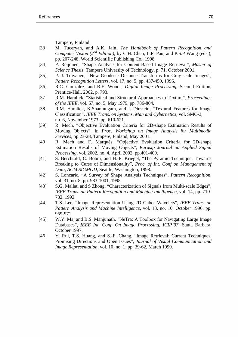
References
70
Tampere, Finland. [33] M. Tuceryan, and A.K. Jain, The Handbook of Pattern Recognition and
Computer Vision (2nd Edition), by C.H. Chen, L.F. Pau, and P.S.P Wang (eds.), pp. 207-248, World Scientific Publishing Co., 1998.
[34] P. Reijonen, “Shape Analysis for Content-Based Image Retrieval”, Master of Science Thesis, Tampere University of Technology, p. 71, October 2001.
[35] P. J. Toivanen, “New Geodesic Distance Transforms for Gray-scale Images”, Pattern Recognition Letters, vol. 17, no. 5, pp. 437-450, 1996.
[36] R.C. Gonzalez, and R.E. Woods, Digital Image Processing, Second Edition, Prentice-Hall, 2002, p. 793.
[37] R.M. Haralick, “Statistical and Structural Approaches to Texture”, Proceedings of the IEEE, vol. 67, no. 5, May 1979, pp. 786-804.
[38] R.M. Haralick, K.Shanmugam, and I. Dinstein, “Textural Features for Image Classification”, IEEE Trans. on Systems, Man and Cybernetics, vol. SMC-3, no. 6, November 1973, pp. 610-621.
[39] R. Mech, “Objective Evaluation Criteria for 2D-shape Estimation Results of Moving Objects”, in Proc. Workshop on Image Analysis for Multimedia Services, pp.23-28, Tampere, Finland, May 2001.
[40] R. Mech and F. Marqués, “Objective Evaluation Criteria for 2D-shape Estimation Results of Moving Objects”, Eurasip Journal on Applied Signal Processing, vol. 2002, no. 4, April 2002, pp.401-409.
[41] S. Berchtold, C. Böhm, and H.-P. Kriegel, “The Pyramid-Technique: Towards Breaking to Curse of Dimensionality”, Proc. of Int. Conf on Management of Data, ACM SIGMOD, Seattle, Washington, 1998.
[42] S. Loncaric, “A Survey of Shape Analysis Techniques”, Pattern Recognition, vol. 31, no. 8, pp. 983-1001, 1998.
[43] S.G. Mallat, and S Zhong, “Characterization of Signals from Multi-scale Edges”, IEEE Trans. on Pattern Recognition and Machine Intelligence, vol. 14, pp. 710-732, 1992.
[44] T.S. Lee, “Image Representation Using 2D Gabor Wavelets”, IEEE Trans. on Pattern Analysis and Machine Intelligence, vol. 18, no. 10, October 1996. pp. 959-971.
[45] W.Y. Ma, and B.S. Manjunath, “NeTra: A Toolbox for Navigating Large Image Databases”, IEEE Int. Conf. On Image Processing, ICIP’97, Santa Barbara, October 1997.
[46] Y. Rui, T.S. Huang, and S.-F. Chang, “Image Retrieval: Current Techniques, Promising Directions and Open Issues”, Journal of Visual Communication and Image Representation, vol. 10, no. 1, pp. 39-62, March 1999.