• Many factors/inputs/variables must be taken into consideration when making a product especially a brand new one

• The Taguchi method is a structured approach for determining the ”best” combination of inputs to produce a product or service

• Based on a Design of Experiments (DOE) methodology for determining parameter levels

• DOE is an important tool for designing processes and products• A method for quantitatively identifying the right inputs and

parameter levels for making a high quality product or service

• Taguchi approaches design from a robust design perspective

Taguchi Design of Experiments

Taguchi method

• Traditional Design of Experiments focused on how

different design factors affect the average result level

• In Taguchi’s DOE (robust design), variation is more

interesting to study than the average

• Robust design: An experimental method to achieve

product and process quality through designing in an

insensitivity to noise based on statistical principles.

• A statistical / engineering methodology that aim at

reducing the performance “variation” of a system.

• The input variables are divided into two board

categories.

• Control factor: the design parameters in product or

process design.

• Noise factor: factors whoes values are hard-to-control

during normal process or use conditions

Robust Design

4

• The traditional model for quality losses

• No losses within the specification limits!

The Taguchi Quality Loss Function

• The Taguchi loss function

• the quality loss is zero only if we are on target

Scrap Cost

LSL USLTarget

Cost

Example (heat treatment process for

steel)

• Heat treatment process used to harden steel components

• Determine which process parameters have the greatest impact on the hardness of the steel components

unitLevel 2Level 1ParametersParameter

number

OC900760Temperature1

OC/s14035Quenching rate2

s3001Cooling time3

Wt% c61Carbon contents4

%205Co 2 concentration5

Taguchi method

• To investigate how different parameters affect the mean and variance of a process performance characteristic.

• The Taguchi method is best used when thereare an intermediate number of variables (3 to50), few interactions between variables, andwhen only a few variables contributesignificantly.

Two Level Fractional Factorial Designs

• As the number of factors in a two level factorial design

increases, the number of runs for even a single replicate of

the 2k design becomes very large.

• For example, a single replicate of an 8 factor two level

experiment would require 256 runs.

• Fractional factorial designs can be used in these cases to

draw out valuable conclusions from fewer runs.

• The principle states that, most of the time, responses are

affected by a small number of main effects and lower order

interactions, while higher order interactions are relatively

unimportant.

Half-Fraction Designs

• A half-fraction of the 2k design involves running only half of the treatments of the full factorial design. For example, consider a 23 design that requires 8 runs in all.

• A half-fraction is the design in which only four of the eight treatments are run. The fraction is denoted as 2 3-1with the “-1 " in the index denoting a half-fraction.

• In the next figure: Assume that the treatments chosen for the half-fraction design are the ones where the interaction ABC is at the high level (1). The resulting 23-1 design has a design matrix as shown in Figure (b).

Half-Fraction Designs

23

2 3-1

I= ABC

2 3-1

I= -ABC

No. of runs = 8

No. of runs = 4

No. of runs = 4

Half-Fraction Designs

• The effect, ABC , is called the generator or wordfor this design

• The column corresponding to the identity, I , and column corresponding to the interaction , ABCare identical.

• The identical columns are written as I= ABC and this equation is called the defining relation for the design.

Quarter and Smaller Fraction Designs

• A quarter-fraction design, denoted as 2k-2 , consists of a fourth of the runs of the full factorial design.

• Quarter-fraction designs require two defining relations.

• The first defining relation returns the half-fraction or the 2 k-1design. The second defining relation selects half of the runs of the 2k-1 design to give the quarter-fraction.

• Figure a, I= ABCD � 2k-1. Figure b, I=AD� 2k-2

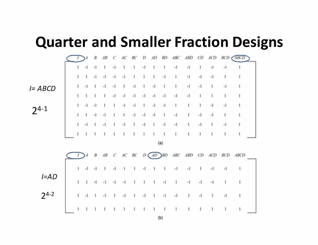
Quarter and Smaller Fraction Designs

I= ABCD

24-1

I=AD

24-2

Taguchi's Orthogonal Arrays

• Taguchi's orthogonal arrays are highly fractional orthogonal designs. These designs can be used to estimate main effects using only a few experimental runs.

• Consider the L4 array shown in the next Figure. The L4 array is denoted as L4(2^3).

• L4 means the array requires 4 runs. 2^3 indicates that the design estimates up to three main effects at 2 levels each. The L4 array can be used to estimate three main effects using four runs provided that the two factor and three factor interactions can be ignored.

Taguchi's Orthogonal ArraysL4(2^3)

2III3-1

I = -ABC

Taguchi's Orthogonal Arrays

• Figure (b) shows the 2III3-1 design (I = -ABC,

defining relation ) which also requires four runs

and can be used to estimate three main effects,

assuming that all two factor and three factor

interactions are unimportant.

• A comparison between the two designs shows

that the columns in the two designs are the same

except for the arrangement of the columns.

Taguchi’s Two Level Designs-Examples

L8 (2^7)

L4 (2^3)

Taguchi’s Three Level Designs- Example

L9 (3^4)

Analyzing Experimental Data

• To determine the effect each variable has on the output, the signal-to-noise ratio, or the SN number, needs to be calculated for each experiment conducted.

• yi is the mean value and si is the variance. yi is the value of the performance characteristic for a given experiment.

signal-to-noise ratio

Worked out Example

• A microprocessor company is having difficulty with its current yields. Silicon processors are made on a large die, cut into pieces, and each one is tested to match specifications.

• The company has requested that you run experiments to increase processor yield. The factors that affect processor yields are temperature, pressure, doping amount, and deposition rate.

• a) Question: Determine the Taguchi experimental design orthogonal array.

Worked out Example…

• The operating conditions for each parameter and level are listed below:

•A: Temperature•A1 = 100ºC •A2 = 150ºC (current) •A3 = 200ºC

•B: Pressure•B1 = 2 psi •B2 = 5 psi (current) •B3 = 8 psi

•C: Doping Amount•C1 = 4% •C2 = 6% (current) •C3 = 8%

•D: Deposition Rate•D1 = 0.1 mg/s •D2 = 0.2 mg/s (current) •D3 = 0.3 mg/s

Selecting the proper orthogonal array by

Minitab Software

Example: select the appropriate design

Example: select the appropriate design

Example: enter factors’ names and levels

Worked out Example…a) Solution: The L9 orthogonal array should be used.

The filled in orthogonal array should look like this:

This setup allows the testing of all four variables without having to run 81 (=34)

Selecting the proper orthogonal array by

Minitab Software

Worked out Example…

• b) Question: Conducting three trials for each

experiment, the data below was collected.

Compute the SN ratio for each experiment for

the target value case, create a response chart,

and determine the parameters that have the

highest and lowest effect on the processor

yield.

Worked out Example…

Standar

d

deviatio

nMean Trial 3Trial 2Trial 1

Deposit

ion

Rate

Doping

Amoun

t

Pressur

e

Temper

ature

Experi

ment

Numbe

r

8.580.170.782.387.30.1421001

5.969.663.270.774.80.2651002

5.852.445.754.956.50.3881003

9.773.462.378.279.80.3621504

12.769.654.976.577.30.1851505

386.583.287.3890.2481506

4.760.955.762.364.80.2822007

5.993.287.393.2990.3452008

6.87163.27475.70.1682009

Enter data to Minitab

Worked out Example…

• b) Solution:

For the first treatment, 5.195.8

1.80log10

2

2

==SN i

SNiT 3T 2T 1

D

(dep)

C

(dop)

B

(pres)

A

(temp)

Experiment

Number

19.570.782.387.311111

21.563.270.774.822212

19.145.754.956.533313

17.662.378.279.832124

14.854.976.577.313225

29.383.287.38921326

22.355.762.364.821137

24.087.393.29932238

20.463.27475.711339

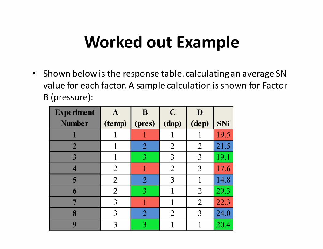
Worked out Example

• Shown below is the response table. calculating an average SN

value for each factor. A sample calculation is shown for Factor

B (pressure):

SNi

D

(dep)

C

(dop)

B

(pres)

A

(temp)

Experiment

Number

19.511111

21.522212

19.133313

17.632124

14.813225

29.321326

22.321137

24.032238

20.411339

Worked out Example

Level A (temp) B (pres) C (dop) D (dep)

1 20 19.8 24.3 18.2

2 20.6 20.1 19.8 24.4

3 22.2 22.9 18.7 20.2

2.2 3.1 5.5 6.1

Rank 4 3 2 1

8.193

3.226.175.19B1 =

++=SN 1.20

30.248.145.21

B2 =++

=SN

9.223

4.203.291.19B3 =

++=SN

1.38.199.22 =−=−=∆ MinMax

The effect of this factor is then calculated by determining the range:

∆

Deposition rate has the largest effect on the processor yield

and the temperature has the smallest effect on the processor yield.

Example solution by Minitab

Example: determine response columns

Example Solution

Example: Main Effect Plot for SN

ratios

Differences between SN and Means

response table

Main effect plot for means

Mixed level designs

• Example: A reactor's behavior is dependent upon impeller

model, mixer speed, the control algorithm employed, and the

cooling water valve type. The possible values for each are as

follows:

• Impeller model: A, B, or C

• Mixer speed: 300, 350, or 400 RPM

• Control algorithm: PID, PI, or P

• Valve type: butterfly or globe

• There are 4 parameters, and each one has 3 levels with the

exception of valve type.

Mixed level designs

Available designs

Select the appropriate design

Factors and levels

Enter factors and levels names

Design matrix