tactical choices of medium and high input dairy systems

Tactical Choices of Medium and

High Input Dairy Systems

Courtney Stewart Gronow

A thesis submitted in total fulfilment of the requirements of the degree of

Master of Agriculture

February 2013

Produced on archival quality paper

Department of Agriculture and Food Systems

Faculty of Land and Environment

The University of Melbourne

Victoria, 3010 Australia

ii

Abstract In the last decade dairy farms in northern Victoria were exposed to increased volatility of

input and output prices as well as variable climate conditions that include a big dry

period. Two representative case study pasture based dairy farms of ‘medium’ and ‘high’

input were selected to examine the production and financial outcomes that arise from a

multi-year sequence of tactical farm management decisions.

The approach of the research had several key aspects; case studies were selected as the

method of investigation, on-farm interviews of the case study farmers were carried out

and their financial and physical history was collected. A stochastic multiyear whole-farm

biophysical and economic spreadsheet model was developed to analyse the physical and

economical performance of the case study farms

The study found that both farming systems had different optimum choices available year

to year to increase profitability

In many of the scenarios tested, the decision option with the highest growth in equity

compared to other options tested did not always result in the highest net cash flow. The

decision maker would need to evaluate the net cash flow implications of their decisions to

determine if they are worthwhile choices.

For both farms, in years with greater upside, there was a greater range of outcomes

between decisions compared to years with poor financial outcomes. This suggests farm

managers cannot get too relaxed and complacent in the good years and need to ensure

they are gaining the benefits of the good year as well as minimizing losses in the poor

years.

iii

Declaration This is to certify that

(i) The thesis comprises only my original work except where indicated,

(ii) Due acknowledgment has been made in the text to all other material used,

(iii) The thesis is fewer than 30,000 words in length, inclusive of footnotes, but

exclusive of tables, maps, appendices and bibliography.

Courtney Gronow

February 2013

iv

Acknowledgements The completion of this thesis came with the help and support of many and are worthy of a

big thankyou!

Firstly I would like to thank my supervisors Bill Malcolm and Gordon Cleary for putting

in the time to make this result achievable and I’m very appreciative in the knowledge

gained during the journey.

I am very grateful to the farmers who gave me time and resources to complete the case

studies, their in-depth interviews were a great window into their thought processes on

running their farms.

Dairy Australia were very supportive through my Masters, not only funding but also for

the various opportunities of conferences and other projects.

Finally a big thankyou goes out to all family and friends who have supported and

encouraged well, and put up with many lost weekends.

v

Table of Contents Abstract ............................................................................................................................... ii Declaration ......................................................................................................................... iii Acknowledgements ............................................................................................................ iv Table of Contents ................................................................................................................ v List of Tables ................................................................................................................... viii List of Figures .................................................................................................................... ix 1 Introduction ................................................................................................................. 1 1.1 Background to the Australian dairy industry ...................................................... 1 1.1.1 Volatility of prices ....................................................................................... 1

1.2 Background to the Murray region dairy industry ............................................... 2 1.2.1 Demographics ............................................................................................. 2 1.2.2 Drought and Climate Change on the Murray Dairy region ....................... 3 1.2.3 Irrigation in the Murray Dairy region ........................................................ 4 1.2.4 Exiting the industry ..................................................................................... 5 1.2.5 Production and herd size ............................................................................ 6 1.2.6 Calving pattern ........................................................................................... 6 1.2.7 Pastures and water efficiency ..................................................................... 7 1.2.8 Feeding systems .......................................................................................... 7

1.3 Aim of thesis/Key questions ............................................................................... 9 1.4 Outline of thesis ................................................................................................ 10

2 Farm management and risk ....................................................................................... 11 2.1 Introduction to farm management and risk ....................................................... 11 2.2 Farm Management ............................................................................................ 12 2.3 Risk and uncertainty ......................................................................................... 16 2.3.1 Strategic risks............................................................................................ 18 2.3.2 Operational risks ...................................................................................... 19 2.3.3 Risk mitigation actions .............................................................................. 23

2.4 Analytical approaches to farm management decision making ......................... 25 2.4.1 Comparative analysis................................................................................ 25 2.4.2 Budgeting .................................................................................................. 25 2.4.3 Linear Programming: ............................................................................... 26 2.4.4 Decision theory ......................................................................................... 27 2.4.5 System modelling ...................................................................................... 28 2.4.6 Modelling with Risk Aversion ................................................................... 29

2.5 Key research question ....................................................................................... 31 3 Method ...................................................................................................................... 32 3.1 Introduction ....................................................................................................... 32 3.2 Case studies ....................................................................................................... 32 3.3 Economic analysis ............................................................................................ 35 3.4 Analytical Model .............................................................................................. 36 3.4.1 Overview of the modelling process ........................................................... 37 3.4.2 Assumptions used in the model ................................................................. 38

3.5 Data collection .................................................................................................. 44

vi

3.5.1 Case study farm interview ......................................................................... 44 3.5.2 Farm performance data ............................................................................ 45

3.6 Description of scenario testing.......................................................................... 45 3.6.1 Defining each years season forecast......................................................... 45 3.6.2 Defining each scenario ............................................................................. 46 3.6.3 Stochastic simulation ................................................................................ 46 3.6.4 Comparison of cumulative farm plans ...................................................... 47

3.7 Summary of method .......................................................................................... 48 4 Case study 1 – Medium input farm ........................................................................... 49 4.1 Description of Farm 1 ....................................................................................... 49 4.2 Year 1 Farm 1 analysis ..................................................................................... 51 4.2.1 Year 1 season forecast settings ................................................................. 51 4.2.2 Year 1 options available ........................................................................... 51 4.2.3 Year 1 Farm 1 results and discussion ....................................................... 52

4.3 Year 2 Farm 1 analysis ..................................................................................... 53 4.3.1 Year 2 season forecast settings ................................................................. 53 4.3.2 Year 2 options available ........................................................................... 53 4.3.3 Year 2 Farm 1 results ............................................................................... 54





4.8 Six year cumulative effect of decision making on Farm 1 ............................... 64 4.8.1 Six year cumulative Results for Farm 1 .................................................... 64

4.9 Alternative Strategic option – Sell high security water .................................... 68 4.9.1 Sell high security water results ................................................................. 69

5 Case study 2 – High input farm ................................................................................ 71 5.1 Description of Farm 2 ....................................................................................... 71 5.2 Year 1 Farm 2 analysis ..................................................................................... 73 5.2.1 Year 1 season forecast settings ................................................................. 73 5.2.2 Year 1 options available ........................................................................... 73 5.2.3 Year 1 Farm 2 results ............................................................................... 74

5.3 Year 2 Farm 2 analysis ..................................................................................... 75 5.3.1 Year 2 season forecast settings ................................................................. 75

vii

5.3.2 Year 2 options available ........................................................................... 75 5.3.3 Year 2 Farm 2 results ............................................................................... 75





5.8 Six year cumulative results for Farm 2 ............................................................. 85 6 Comparison of case study Farm 1 to Farm 2 ............................................................ 88 7 Conclusion ................................................................................................................ 91 8 Appendix 1 - Case Study Interview Questionnaire................................................... 95 9 Appendix 2 – Case study Farm 1 .............................................................................. 98 9.1 Probabilistic ranges set for Farm 1 ................................................................... 98 9.2 Farm 1 six year plan Control ............................................................................ 99 9.3 Farm 1 Optimal 6 year alternative .................................................................. 102

10 Appendix 3 – Case Study Farm 2 ....................................................................... 105 10.1 Probabilistic ranges set for Farm 2 ................................................................. 105 10.2 Farm 2 six year plan Control .......................................................................... 106 10.3 Farm 2 six year plan Optimal.......................................................................... 109

11 Reference ............................................................................................................ 112

viii

List of Tables Table 1-1. Milk price and feed costs for Murray Dairy region (Dairy Australia 2009a) ... 2

Table 1-3 Historical high security water allocations for Murray and Goulburn irrigation systems between 2003-04 and 2011-12 .............................................................................. 5

Table 1-4. Farm performance in Lower Murray Darling Basin between 2004 and 2009 (Dairy Australia 2009a) ...................................................................................................... 6

Table 1-5. Proportion of dairy land irrigated in the Murray Dairy Region (Dairy Australia 2009a) ................................................................................................................................. 7

Table 1-6. Average grain consumption (tonnes percow) in Murray Dairy region (Dairy Australia 2009b).................................................................................................................. 8

Table 2-1 Potential strategic risk factors in agriculture (Miller et al. 1998) .................... 19 Table 2-2 Business risks (Miller et al. 2004; White 2002) ............................................... 20

Table 2-3 The universe of risk: Taxonomy of risks facing Australian dairy farms. ......... 22

Table 4-1 Return on assets managed for ‘control’ and ‘optimal’ pathways ..................... 66

Table 5-1 Return on assets managed for control and optimal pathway of Farm 2 ........... 86

Table 9-1 Physical assumptions for Control Farm 1 ........................................................ 99

Table 9-2 Price assumptions for Control Farm 1 ............................................................ 100

Table 9-3 Balance sheet options Control Farm 1............................................................ 100

Table 9-4 Profit and loss statement Control Farm 1 ....................................................... 101

Table 9-5 Cash flow statement Control Farm 1 .............................................................. 101

Table 9-6 Physical assumptions Optimal Farm 1 ........................................................... 102

Table 9-7 Price assumptions Optimal Farm 1................................................................. 103

Table 9-8 Balance sheet Optimal Farm 1 ....................................................................... 103

Table 9-9 Profit and loss statement Optimal Farm 1 ...................................................... 104

Table 9-10 Cash flow statement Optimal Farm 1 ........................................................... 104

Table 10-1 Physical assumptions Control Farm 2 .......................................................... 106 Table 10-2 Price assumptions Control Farm 2 ............................................................... 107

Table 10-3 Balance sheet Control Farm 2 ...................................................................... 107

Table 10-4 Profit and loss statement Control Farm 2 ..................................................... 108

Table 10-5 Cash flow statement Control Farm 2 ............................................................ 108

Table 10-6 Physical assumptions Optimal Farm 2 ......................................................... 109

Table 10-7 Price assumptions Optimal Farm 2............................................................... 110

Table 10-8 Balance sheet Optimal Farm 2 ..................................................................... 110

Table 10-9 Profit and loss statement Optimal Farm 2 .................................................... 111

Table 10-10 Cash flow statement Optimal Farm 2 ......................................................... 111

ix

List of Figures Figure 1-1. Long-term nominal feed grain price trends for Victoria in dollars per tonne Source: Dairy Australia (2009b) ......................................................................................... 2

Figure 1-2 Kyabram mean annual rainfall for years 2000 to 2011 ('Bureau of Meteorology 2013).............................................................................................................. 3

Figure 1-3 Kyabram mean monthly rainfall (mm) 2000-2009 compared to 1964-2012 .... 4

Figure 1-4 Nominal trading temporary water price and volume traded for Goulburn system between Jan 2005 to May 2012 (Dairy Australia 2012) ......................................... 5

Figure 2-1 A classification diagram of farmer decisions (derived from Boehlje and Eidman (1984) and Dryden (1997) - Source Gray et al. (2009) and Tarrant and Malcolm (2011))............................................................................................................................... 14 Figure 2-2. A qualitative approach to expected value (Benson 1999) .............................. 18

Figure 3-1 Description of the method of how the management options were assessed (Red line is the Control pathway whereby Option 1 was selected every year and the Blue line is the Optimal pathway whereby the most favourable option was chosen every year. All outcomes in the following years for each pathway were derived from the chosen precedent options. ............................................................................................................. 47

Figure 4-1 Growth in equity of three alternative options for Year 1 Farm 1.................... 52


Figure 4-3 Growth in equity of five alternative options for Year 3 Farm 1 ..................... 56

Figure 4-4 Growth in equity of five alternative options for Year 4 Farm 1 ..................... 59


Figure 4-6 Growth in equity of four alternative options for Year 6 Farm 1 ..................... 63

Figure 4-7 Six year cumulative discounted growth in equity of ‘control’ and ‘optimal’ pathways for Farm 1 (Medium input) ............................................................................... 65

Figure 4-8 Six year cumulative discounted growth in equity for control and optimal pathways with and without the sale of 500 ML of high security water right and with and without the purchase of low security water right in Year 1 .............................................. 69


Figure 5-2 Growth in equity of two alternative options for Year 2 Farm 2 ...................... 76



Figure 5-5 Growth in equity of two alternative options for Year 5 Farm 2 ...................... 83


Figure 5-7 Six year cumulative discounted growth in equity of control and optimal pathway of Farm 2 (High input) ....................................................................................... 85

Figure 6-1 Return on Assets managed for the Optimal pathways of Farm 1 and 2 .......... 88

1 Introduction

1.1 Background to the Australian dairy industry

The Australian dairy industry is one of Australia’s major rural industries. It had a

production farm gate value of 3.9 billion in 2010-11 and directly employs an approximate

of 40,000 people on dairy farms and manufacturing plants. The industry experienced

strong growth through the 1990s, however was hit by drought and ongoing dry conditions

during the 2000s with also increasing levels of market volatility.

1.1.1 Volatility of prices

There is consensus in the literature (Ashton and Mackinnon 2008; Dairy Australia 2008;

Wales et al. 2006) that prices for outputs and inputs in the dairy industry are becoming

more volatile. Ashton and Mackinnon (2008) found that since the deregulation of farm-

gate milk pricing arrangements in July 2000, the average prices received by Australian

dairy farmers have been more volatile than in the preceding decade, partly as a result of

the markets greater exposure to international price fluctuations and exchange rates. Wales

et al. (2006) noted that the volume of dairy products traded is small relative to world

productive capacity, and as a result, creates significant shifts in prices paid for dairy

products over short time periods. Changes in exchange rates has also has impact on farm

gate prices. The Department of Primary Industries of Victoria (2009, p.8) states that “a 1

cent appreciation of the $AUD against the $USD results in a reduction in farm gate prices

of 0.5-0.6 cents per litre.” During the 2008/2009 season, the effects of the economic

financial crisis on global dairy commodity prices caused a significant drop in prices of

over 50 % (Department of Primary Industries 2009).

A graph of barley and wheat prices in Victoria between 1984 and 2008 is shown in

Figure 1-1. It shows that prices are more volatile in the later half of the period as opposed

to the first half. Table 1-1 shows the milk, purchased grain or concentrate and purchased

fodder price between 2003-04 and 2008-09 in the Murray Dairy region. The average milk

2

price received by farmers had a low of $3.60 in 2003-04 and a high of $6.53 in 2007-08.

Purchased fodder price was also highly variable, with the lowest average price of $137 in

2004-05 and a high of $283 in 2007-08, which is more than double.

Figure 1-1. Long-term nominal feed grain price trends for Victoria in dollars per tonne Source: Dairy

Australia (2009b)

Table 1-1. Milk price and feed costs for Murray Dairy region (Dairy Australia 2009a)

2003-04 2004-05 2005-06 2006-07 2007-08 2008-09

Received milk price 3.6 4.31 4.42 4.2 6.53 4.64

$/kg MS

Purchased grain / conc. 264 221 248 309 364 350

$/t

Purchased fodder 163 137 138 208 283 250

$/t

1.2 Background to the Murray region dairy industry

1.2.1 Demographics

With an average rainfall of 400 mm per year in the Murray Dairy region (Bethune and

Armstrong 2004) and evaporation of 1200-1300 mm per year for irrigated perennial

pasture (Austin 1998), the area relies heavily on irrigation for pasture growth. However,

water allocations are becoming more volatile and consequently both permanent and

temporary water costs are also becoming more volatile (Lawson et al. 2009). The dairy

3

industry in the Murray Dairy region has seen higher volatility of input prices (grain, hay,

water and fertiliser) and output prices (milk) since the start of the decade.

The number of dairy farms in Victoria has been gradually decreasing, falling from 11,467

registered dairy farms in 1979-80 to 5,159 in 2009-10,(Dairy Australia 2011a) while

productivity and herd size have both increased 30 % in the last 10 years (Bethune and

Armstrong 2004). There were only 2,589 dairy farms in the Lower Murray-Darling Basin

in 2006-07, 30 % of the total number of dairy farms in Australia (ABS 2008).

1.2.2 Drought and Climate Change on the Murray Dairy region

The Murray Dairy region has been ravaged by drought over the previous decade. Figure

1-2 shows the annual average rainfall for the previous decade 2000 to 2011. Only 3 years

were slightly higher than the average rainfall. FigureFigure 1-3 shows the average

monthly rainfall for Kyabram for the 2000 to 2009 period compared to the long term

averages. Most months were below the average monthly rainfall with the exception of

some summer months. At least 95 % of the Murray Dairy region was drought-affected

between 2003-04 and 2008-09 (Dairy Australia 2009a).

Figure 1-2 Kyabram mean annual rainfall for years 2000 to 2011 (Bureau of Meteorology 2013)

4

Figure 1-3 Kyabram mean monthly rainfall (mm) 2000-2009 compared to 1964-2012

1.2.3 Irrigation in the Murray Dairy region

From the middle of the last century until the 1980s, irrigation water allocations averaged

around 190 %, with a low of 130 % experienced in the 1982 drought (Poole 2009). Then,

from the mid-1980s to the mid-1990s, allocations started to reduce, falling to an average

of 180 %. Allocations reduced further to an average of 160 % between 1995 and 2005,

with a low of 57 % in the Goulburn system in the 2002-03 drought (Poole 2009). Table

1-2 shows the declining allocations between 2005-06 and 2008-09, then an increase back

to 100 % allocations thereafter. Figure 1-4 shows the volume and nominal trading value

of temporary water in the Goulburn system from 2005 to 2012. At the height of the

drought, temporary water traded at over $1,000 per ML in 2007. Poole (2009) states that

the sharp changes in water allocation were due to the continued development of the

irrigation system over the previous fifty years peaking at the same time as a big dry

period, making the shortfall seem more a function of the drought than something that

would have inevitably happened.

5

Table 1-2 Historical high security water allocations for Murray and Goulburn irrigation systems

between 2003-04 and 2011-12

Figure 1-4 Nominal trading temporary water price and volume traded for Goulburn system between

Jan 2005 to May 2012 (Dairy Australia 2012)

1.2.4 Exiting the industry

A study by Barr (2005) found that in 1981, people leaving the dairy industry in Victoria

had usually passed the age of 55 years. By 2001, younger people were more likely to be

leaving the industry and people over 55 were half as likely to leave the industry

compared to those of that age in 1981. The number of dairy farmers older than 45 had

changed little since 1976, but the number of dairy farmers under the age of 45 had

halved. As a result, the median age of dairy farmers in the Goulburn Murray irrigation

district had increased from 41 in 1981 to 47 in 2000 (Dairy Australia 2009c). The exit

2003-04 2004-05 2005-06 2006-07 2007-08 2008-09 2009-10 2010-11 2011-12

Irrigation allocation 100% 100% 144% 95% 57% 35% 100% 100% 100%

- Murray

Irrigation allocation 100% 100% 100% 29% 43% 31% 71% 100% 100%

- Goulburn

6

rate for Victorian dairy farmers has averaged between six and seven per cent per annum

between 1976 and 2001, with an exception between 1991 and 1996 at 4.5 % (Barr 2005).

1.2.5 Production and herd size

The number of dairy cattle in the Lower Murray-Darling Basin has changed little

between 1993-94 and 2006-07. There were around 700,000 cattle in 1993-94 and 695,000

in 2006-07 (ABS 2009). However, there was a 13.5 % drop in cattle head in the 2007-08

season, back to 600,000 head (ABS 2009). The Loddon area had the largest decline in

dairy cattle population, a reduction of 87.2 % from 1993-94 to 2007-08, and the Murray

area had the largest increase in cattle population of 53.6 % (ABS 2009). Table 1-3 shows

average cow numbers per farm increased between 2004 and 2006 to remain around 250

between 2006 and 2009 (Dairy Australia 2009a). Average production per farm increased

for each year between 2004 and 2009 with the exception of 2007.

Table 1-3. Farm performance in Lower Murray Darling Basin between 2004 and 2009 (Dairy

Australia 2009a)

2004 2005 2006 2007 2008 2009

Cow numbers 204 246 253 251 260 249

(average per farm)

Milk production 94,000 99,000 104,000 93,000 106,000 112,000

(kg milk solids)

Milk production 1,125,000 1,333,000 1,480,000 1,260,000 1,420,000 1,500,000

(litres)

Farm area (ha) 203 232 167 202 149* 144*

* Dairy Land only

1.2.6 Calving pattern

Farms in the Murray Dairy region have had a shift in calving pattern from seasonal

calving in Spring alone, to split calving between the Spring and Autumn. This is due to

seasonal milk payment incentives and poor reproductive performance (Wales et al.

2006). For the 2007-08 season, ABARE (2009) surveyed northern Victorian and Riverina

7

dairy farmers and found 45 % of farmers undertake seasonal calving, 21 % split calving,

and 34 % year round calving.

1.2.7 Pastures and water efficiency

The biggest issue in the Murray Dairy region over the last decade was drought, with less

irrigation water available and high costs of temporary water purchase. The area was

traditionally sown to perennial pastures for grazing dairy cows, at 70-80 % of the

irrigated milking area. Annual pastures occupied ~20-30 % and other forage crops

consisting of mainly Lucerne and maize occupied 2 % (Armstrong et al. 1998). Table 1-4

shows the decline in the proportion of land irrigated on an average Murray Dairy region

farm.

Table 1-4. Proportion of dairy land irrigated in the Murray Dairy Region (Dairy Australia 2009a)

2004 2005 2006 2007 2008 2009

Proportion of dairy n.a. 63% 72% n.a. 31% 38%

Land irrigated

In the low water allocation seasons, the water use efficiency of pastures became more

important. Grazing of cereal crops has increased and there has been a shift from perennial

pastures to annual pastures in dry seasons.

Lawson et al. (2009) conducted an experiment measuring water productivity (annual dry

matter removed divided by the annual water input consisting of irrigation and rainfall less

runoff (Meyer 2005)) of annual pastures and perennial pastures. The water use efficiency

was higher for the annual pastures (30-37 kg DM/ha.mm) compared to perennial pastures

of (21-27 kg DM/ha.mm).

1.2.8 Feeding systems

A survey by Dairy Australia (2009b) showed that 25 % of respondents in northern

Victoria and Riverina use a partial mixed ration via a permanent or semi-permanent feed

8

pad with their grazed pastures (systems 3 and 4). Huggins (2009) indicated there were

only 28 mixer wagons being used in Victoria and Riverina in 1999, however there has

been a large growth of the use of mixer wagons since then.

In the 2007-08 season, ABARE (2009) surveyed farmers in northern Victoria and

Riverina on their usage of grain, grain mixes and concentrates, finding

- 0 % use less than 0.5 tonnes per cow.

- 28 % (51 RSE) use between 0.5 tonnes to 1.0 tonnes per cow.

- 45 % (34 RSE) use between 1.0 and 2.0 tonnes per cow.

- 26 % (24 RSE) use more than 2.0 tonnes per cow.

- Average for all of northern Victoria and Riverina is 1.48 tonnes per cow (9 RSE).

Table 1-5 shows an increase in average grain consumption (tonnes per cow) in the

Murray Dairy region for the previous 5 years.

Table 1-5. Average grain consumption (tonnes percow) in Murray Dairy region (Dairy Australia

2009b)

2004 2005 2006 2007 2008 2009

Grain consumption (t/cow) n.a. 1.2 1.3 1.4 1.9 1.9

9

1.3 Aim of thesis/Key questions

The increase in volatility of input and output prices over and last decade combined with

the variability in the climate has made the tactical and strategic responsiveness of the

farm decision maker all the more important.

The aim of this thesis is to evaluate the nature and implications of options facing the

managers of two pasture based dairy farm businesses operated at medium and high levels

of input use and trying to minimize losses in unfavourable seasons and maximize profits

in favourable seasons.

This will be investigated by:

• Reviewing farm management, risk and analytical approaches used in decision

making.

• Detailed case study analysis of the approaches of the farm operators and the

management of the biophysical and economic resources of the two farming

systems.

• Evaluate the consequences of the main decision options of these two types of

dairy business, in the farm management context – i.e. technical, human,

economic, financial and risk.

10

1.4 Outline of thesis

In this thesis, an investigation of the biophysical and economic performance of two

different case study farms analysing a multi-year sequence of tactical farm management

decisions is presented. The two case study farms selected were a ‘medium’ input and a

‘high’ input irrigated pasture based dairy farm. The farms had the following profiles:

Case Study Farm 1 – ‘medium’ input

• Current herd size of 300 cows.

• Annual concentrates fed per cow 1.66 tDM.

• Annual pasture grazed per cow 2.7 tDM.

• Current milk production per cow 5400 L. Case Study Farm 2 – ‘high’ input

• Current herd size of 700 cows.

• Annual concentrates fed per cow 2.61 tDM.

• Annual pasture grazed per cow 3.3 tDM.

• Current milk production per cow 7900 L. The case studies were analysed with varying climatic and economic conditions imposed

on them over a six year period. A number of various management decision options were

examined for the case studies and the growth in equity, net cash flow and return on asset

are measured.

In Chapter two the key literature about farm management, decision- making and risk is

canvassed. The Method is set out in Chapter three. The two case study farms are detailed

and analysed in Chapters four and five. Cross case analysis is presented and discussed in

Chapter six. Some conclusions are given in Chapter seven.

11

2 Farm management and risk

2.1 Introduction to farm management and risk

Dairy farm management combines routine operations with complex decision making that

is often based on imperfect information. Farm managers face uncertainty in their

decisions due to factors including the prediction of climate, market movements in input

and output prices and the biological responses they can achieve on farm. Decisions must

be made before the occurrence of an event, without the benefit of hindsight. Farm

business decision-making has been described as gambling against nature and markets

where the odds of many potential events and outcomes are unknown and unknowable

(Tarrent and Malcolm 2011).

Risk is often an unavoidable element in making farm management decisions due to the

nature of farming. According to Anderson et al. (1977, p.3), ‘when a person is uncertain

about the consequences of his decision, we can say he faces a risky choice.” Risk is part

of the many complexities of dairy farm management but risk can also be accounted for in

selecting between risky alternatives and can be managed to suit the farmer’s personal

preferences.

Good management allows a business to function efficiently and allows for growth,

development and wealth creation. Hardaker et al.(1971, p.78) believes that good

management ‘…implies acting with purpose, imagination, forethought and common

sense. It involves forming balanced judgements. In short, it involves making rational

decisions.”

Rational decisions require information about the options and an analysis and evaluation

process for testing these options. This review examines aspects of decision-making under

risk and discusses the merits of different methods used to assess and evaluate alternative

options.

12

2.2 Farm Management

Boehlje and Eidman (1988, p.123) define farm management as “the allocation of limited

resources to maximize the farm family’s satisfaction”. Boehlje (1993) has identified 12

strategic management concepts that are necessary for successful farm management over

the long term:

1. Planning, implementation and control of production, marketing and finance.

2. Low cost commodity production.

3. Ability to spread fixed costs over more output.

4. A focus on profit margins rather than prices.

5. Learning how to obtain the best price and service combination when purchasing

inputs.

6. Developing a marketing plan to maximize returns.

7. Undertaking strategic planning and contingency plans for different scenarios.

8. Assess and manage potential risks.

9. Capital structure (debt and equity).

10. Measurement and control of performance for correction of deviations from plan.

11. Negotiation skills and ability to foster effective interpersonal relationships.

12. Openness to innovative new ideas, technologies and organisations.

Hardaker et al.(1971, p.77), along similar lines, identifies six key decision areas for farm

managers:

1. Technical decisions: what to produce and how to produce it.

2. Trading decisions: what to buy or sell, when, how, and at what price.

3. Financial decision: obtaining and using capital and credit wisely.

4. Accounting aspects: keeping proper records and accounts, or seeing that they are

kept, as required for tax and other purposes. Also ensuring debts are paid and that

money owing is collected.

5. Legal aspects: keeping within the law (or at least, not being found out!).

13

6. Personnel management: hiring and firing workers, directing and supervising the

work of employees.

Makeham (1971, p.23) defines six steps that are central to the farm decision-making

process and which are applicable to both short term and long term decisions:

1. getting ideas and recognising problems.

2. making observations and collecting facts.

3. analysing observations then formulating potential solutions to problems.

4. making the decision.

5. acting on the decision.

6. taking responsibility for the decision.

Boehlje and Eidman (1984) break down management, and thus areas of decision process

or sub-process, into the functions of planning, implementation and control in the farm

management fields of production, finance, human resources and marketing.

Tarrant and Malcolm (2011) differentiate decisions by the time dimension of the matter

the decision is about. Decisions made by farmers are categorised into three groups,

according to the nature, impact, frequency, consequence and ease of reversing the

decision. These groups are operational decisions, tactical decisions and strategic

decisions.

Operational decisions concern day-to-day matters where impact is direct and short term

and can be changed relatively quickly if circumstances change. Examples are choosing

feed allocations for livestock, or identifying and treating diseases.

Tactical decisions are made for the short to medium term, usually within a seasonal or

annual production cycle. Such decisions include setting production and herd size targets

and making choices about purchasing irrigation water, rates of fertiliser application or

levels and type of fodder to achieve the set production targets. These decisions have

14

substantial consequences within the season, but should not have too many impacts in the

medium-long term.

Strategic decisions typically involve major changes to systems and usually require a high

level of analysis and evaluation since capital spending is almost always involved. The

impact of a strategic decision is substantial and has a consequence beyond a single

production period. Examples include purchasing new land or making significant

infrastructure investments.

Gray et al (2009) introduced the notion of ‘structuredness’ of decision making,

suggesting that the experience of the farm manager will also influence the way s/he

approaches a decision. Figure 2-1 provides a representation of the various levels of

farmer decision making, based upon the concepts described above.

Figure 2-1 A classification diagram of farmer decisions (derived from Boehlje and Eidman (1984)

and Dryden (1997) - Source Gray et al. (2009) and Tarrant and Malcolm (2011))

Structured decisions are familiar - the farm manager has experience of both situations and

his choices. Unstructured decisions are unfamiliar – an inexperienced farmer may need to

source and process external information before determining a course of action. Other

decisions, arising from a constantly changing environment, both natural and economic,

15

will be semi-structured, requiring even an experienced farmer to seek new information

about situations and choices.

The stage of development of a farm business is often tied up with the level of experience

of the farm’s operators and the resources that they control at the time. Novice farmers

may tend to focus primarily on production and marketing decisions (items 1 and 2 on the

Hardaker et al.(1971) list, p.12), with experienced farmers tending to focus on other less

immediate but significantly more important matters, such as managing capital, debt and

taxes (items 3-6 on the Hardaker et al.(1971) list, p.12).

Central to farm management decision-making is understanding the differences between

good and bad, and right and wrong decisions. Makeham et al.(1968) state that if there is a

bad outcome, the result is bad, not necessarily the decision. Chapman et al. (2007)

contend that good decisions are made with the best information and judgment available at

the time of decision-making, even if the decision turns out to be wrong. Bad decisions

can be the right decision only with good luck.

“A good decision is a considered choice based on a rational interpretation of the available

information” (Anderson et al. 1977, p.3). However, in the ‘real world’, according to

Makeham et al. (1968, p.1), decisions have to be made ‘…without the benefit of

hindsight, and since hindsight is essential if perfect decisions are to be made, it’s

impossible to guarantee that both the decision and its result will be the best possible.”

For any particular decision maker and any particular decision problem, decision analysis,

according to Anderson et al.(1977, p.12), involves:

1. Defining relevant acts and states and their consequences.

2. Eliciting prior degrees of belief or probabilities for states and degrees of

preference or utility for consequences.

3. Taking account of whatever further predictive information may be available as a

basis for revising the initial probabilities.

16

4. Selecting the optimal strategy on the basis of maximizing expected utility.

In this way, two farm managers may make different decisions even though they are faced

with exactly the same situation. Different farmers often desire different things out of life.

For some, it is the satisfaction of rural living, independence and the maximisation of

income. For others, it may be their family. Good farm management decisions are made

in light of what the farmer’s goals are or what they wish to achieve out of life (Makeham

et al. 1968).

Combined, the above authors describe the complexity involved and the features that need

to be understood and accounted for in establishing a good farm management decision-

making platform. Over time, competition amongst farmers will reduce profit margins and

will place even more pressure on farmers to include capability in the full range of

business, financial and marketing concepts within their management skills set. This is

certainly true in accounting for risk and uncertainty in farm decisions under volatile

climatic and market conditions, since these involve unstructured or semi-structured

decisions for all farmers.

2.3 Risk and uncertainty

(Chapman et al. 2007) state that risk is viewed by people outside farming as something to

be minimized. Farmers on the other hand understand that minimizing risk minimizes

returns as well, so risk is a source of above average profits – and losses. “The existence

of risk and uncertainty creates opportunities and rewards that people are in business to

capture. If the future was known with certainty, the profits would have already been

made.”(Chapman et al. 2007, p.478).

The terms ‘risk’ and ‘uncertainty’ have been used interchangeably (Backus et al. 1997;

Hardaker et al. 1991; Knight 1921; Pannell et al. 2000). Uncertainty involves a situation

where the decision maker does not know the probability of the outcomes and further still

may not know all of the outcomes that may be possible before making a decision.

Hardaker et al. (1991, p.9) state that “uncertainty is important because it affects the

17

consequences of decisions in ways that decision makers are not indifferent about. Such

uncertainty in consequences is called risk, and most people are averse to risk.”

Uncertainty can lead to difficulties in risk management. Cox (2008) states that you cannot

categorise severity ratings for an event that has uncertain consequences. Boehlje (2003,

p.3) states that variation is the measure of risk, namely “the typical way that uncertainty

and the potential loss exposure that results are measured is the range or variability in

particular events or outcomes.”

It is also important to define what risk is not, as risk implies randomness. Predictable

cyclic trends are not risk (Coble and Barnett 2008). In a farming context, a familiar cyclic

trend is seen when grain prices drop during harvest, then rise post-harvest.

According to Miller et al. (2004), there are three ways to interpret risk when it is said that

one particular strategy has more risk compared to other optional strategies. Firstly, more

risk is the higher likelihood of an adverse outcome, hazard or potential loss. Secondly,

risk refers to the size and scale of the loss if it were to occur. Thirdly, more risk may refer

to the expected value of the loss. Expected value is the likelihood of an event occurring

(probability) multiplied by the size of the loss or gain (impact). Unacceptable risk may

result from an event that has a very low probability of occurring, but would create losses

on a large scale. A flood in Northern Victoria has a low probability of occurring but a

high impact on a grass-based dairy farm if it occurs. Unacceptable risk may also arise

from a relatively modest loss that keeps on re-occurring.

Expected value is a common way of expressing quantitative risk assessment. It is used in

the Australian and New Zealand standard for risk management (AS/NZS 2004) whereby

the expected value of individual risks are identified and assessed, then ranked to measure

the relative importance of each risk.

A risk matrix is another tool used for the calculation of expected value. Cox (2008)

explains that a risk matrix is a Table with the categories of “probability,” “likelihood,” or

18

“frequency” for one axis of the Table, and several categories of “severity,” “impact,” or

consequences” on the other axis of the Table. Figure 2-2 from Benson (1999), shows a

descriptive version of an expected value matrix.

Figure 2-2. A qualitative approach to expected value (Benson 1999)

However, one problem with risk matrices is that there is very little rigorous empirical or

theoretical study on how well risk matrices improve risk management decisions (Cox

2008). Hardaker and Lien (2007) state there are problems with conventional risk

assessment. They believe risk aversion is consistently not dealt with, and some risks may

not have a specific adverse event. Also, the severity of possible adverse consequences

can sometimes be uncertain.

2.3.1 Strategic risks

Risk can be categorized into strategic risks and operational risks. Miller et al. (2004) note

that strategic risks are becoming more important as agriculture becomes more

industrialised; however, they are also more difficult to manage than operational risks.

“The focus of strategic risk is the sensitivity of the strategic direction and the ultimate

value of a company to uncertainties in the business climate” (Miller et al. 2004, p.4).

These uncertainties are summarized in Table 2-1.

19

This is not the only possible categorisation of these risks. Various authors include these

strategic risks in their business risk category (Chapman et al. 2007; Makeham and

Malcolm 1993).

Table 2-1 Potential strategic risk factors in agriculture (Miller et al. 1998)

Source

Australian farm products.

Competitive conditions - Producers competing with tariffs and subsidies overseas

Technological uncertainty- Y2K Bug

Industrialization - Older production systems becoming obsolete

Natural - Access to irrigation water is threatened by demands of fast growing cities

Social - Citizens decide that a popular animal production practice is not humane

- Farming is perceived as inefficient water use

Macro-Economics - Value of the dollar rises relative to other countries

Government regulation - EPA limits nitrogen use on farm fields

International - Political unrest in another country leads to economic sanctions against

Government policy - Change in exceptional circumstances aid

- Changes in legislation on tax

Hypothetical Examples

With most strategic risks, it is not possible to manage or transfer them through futures

markets or insurance markets. “Creative strategies must be developed to manage strategic

risk exposure; approaches that include flexibility, adaptability, and diversification”

(Miller et al. 1998, p.15).

2.3.2 Operational risks

Operational risks can be split into business risks and financial risks. (Boehlje 2003).

20

2.3.2.1 Business risks

Business risks refer to those risks that are independent of the way the business is

financed. Thus, the individual business risks are the same irrespective of the amount of

financing or equity (Boehlje 2003). Some business risks are summarised in Table 2-2.

Table 2-2 Business risks (Miller et al. 2004; White 2002)

Business Risk

disease, insects and other pests

management and health expenses

Personal risk - Health of family members, income loss from missing labour and or

Legal risk - Tort liabilities, tax, environment issues

Relation risk - Uncertainty of business dealing partners, eg. action of bank

Also the speed of technological change, a large investment in a

technology could soon be obsolete

computer calculation, new machinery model etc.

Technological risk - Uncertainty of a new technology, eg. new crop variety, chemical,

Casualty risk - Damage or losses to property due to flood, fire, wind, theft…

Price risk - Price fluctuations in both inputs and outputs

Production risk - Uncertainty in production due to variations in weather,

Description

2.3.2.2 Financial risk

Financial risk is the added variability of the net returns of the business as a result of the

financial obligation required with debt financing (Miller et al. 2004). Debt leveraging

multiplies the potential financial gains or losses of a business.

Boehlje (2003, p.4) states that there are intrinsic risks in using debt. “Uncertainty

associated with the cost and availability of debt is reflected partly in fluctuations in

interest rates for loans and partly through non-price sources. Non-price sources, a type of

institutional uncertainty, include differing loan limits, security requirements, and

21

maturities, which impact on the availability of loan funds over time. Thus, financial risk

also includes uncertain interest rates and uncertain loan availability.”

2.3.2.3 Australian dairy farm risk taxonomy

Table 2-3 provides a broader perspective of the strategic and operational risks that

Australian dairy farmers face, whether directly within their farm businesses or indirectly

through their supplied milk factory.

22

Table 2-3 The universe of risk: Taxonomy of risks facing Australian dairy farms. Adapted from (Miller et al. 2004)

Categories of Risk

- High debt servicing capacity, leverage, debt structure, non

-equity financing, liquidity, solvency and profitability

- Product price volatility, input price volatility, cost structure

Contract terms, market outlets and access

- Contractual risks, interdependency, confidentiality, cultural

conflict

- Market share, pricing wars

- Product liability, credit risk, poor market timing, inadequate

customer support

- Transportation, service availability, cost, dependence on

distributors

- Employees, independent contractors, training, staffing

adequacy

- Civil unrest, war, terrorism, enforcement of intellectual property

rights, change in leadership that revises economic policies

- Reporting and compliance, environmental

- Corporate image, brands, reputations of key employees

- Mergers and acquisitions, joint ventures and alliances,

flexibility resource allocation and planning, organisational agility

- Complexity, obsolescence, workforce skill set

- Foreign exchange, portfolio, cash, interest rate

- Facilities, contractual risks, natural hazards, internal processes

and controls

Financial markets and

instruments

Distribution systems

and channels

Competitors and

competition

Customers and

customer relations

Illustrative sources of risk

Financing and

financial structure

Market prices and

terms of trade

Operations and

business practices

Business partners and

partnerships

Technological factors

Strategic position and

Reputation and image

Political factors

People and human

resources

Regulatory and

legislative factors

23

2.3.3 Risk mitigation actions

Managers have a variety of methods for managing operational and strategic risks,

depending upon the nature of the risk involved. Four common methods of managing risks

are avoidance, reduction, assumption or retention, and transfer (Miller et al. 2004).

2.3.3.1 Avoidance of risk

Risk avoidance involves structuring the business so that it can avoid, or eliminate

particular risks completely. At the operational level, an example of risk avoidance on a

dairy farm might concern how replacement stock is acquired. The farmer may choose to

avoid exposing the business to the risks of raising replacement stock on-farm and simply

buy his replacement stock. This reduces all of the risks associated with raising

replacement stock, but may introduce new risks such as price risk on the replacement

stock and exposing your herd to new diseases.

At a strategic level, one way to avoid the spectrum of risks in dairying is to leave the

dairy industry altogether. Many farmers have chosen this approach. There have been

6,121 dairy farms deregistered in Victoria between 1979-80 and 2006-07 (Dairy Australia

2008).

Tactically, over the last decade, many Murray Dairy region farmers have attempted to

avoid water-related risks by reducing the area of perennial-based pastures on their farms

and increasing the area of more water-efficient annual pastures and crops.

2.3.3.2 Reduction of risk

Managing risks by reduction involves lowering the risks a business faces. A ruminant

nutritional advisor may supply timely expert advice to the dairy farmer that reduces but

does not eliminate the incidence of health problems in the herd but, if the advice involves

24

new costs, “this reduction of risk may result in implicit or explicit reductions in net

returns” (Miller et al. 2004).

Another way to reduce risk is to diversify. This can be achieved by changing the

enterprise mix on a farm e.g. adding beef production into a dairying operation. Another

example of diversification may involve purchasing feeds from different geographical

areas or producers to decrease the farm’s exposure to fodder quality risk.

2.3.3.3 Assumption or retention of risk

Assumption or retention of risk occurs when specific risks are accepted into the business,

as there is a compensatory offset through increased control over production and or

enhanced overall profitability. An example of risk assumption is associated with feeding

grain to dairy cows. Price risk and production risk are known to be associated with grain

feeding; however, many dairy farmers accept these risks for rewards in extra milk

production, increased income, altered milk components, increased herd fertility, and herd

health benefits.

2.3.3.4 Transfer of risk

Managing risk by transfer involves one party transferring the risk to another party,

usually for a fee. This may be through insurance, futures or options contracts. This can

also include actions such as storing grain on-farm to eliminate intra-year volatility in

grain price.

Nationally, there has been an increase in transferring risk in grain price, with the

proportion of farmers forward contracting for later delivery increasing from 13 % in 2006

to 21 % in 2008 to 23 % in 2009 (Dairy Australia 2009b).

25

2.4 Analytical approaches to farm management decision making

In order for a farmer to undertake a sound decision-making process, s/he has to decide

what type of decision analysis is appropriate to help with the choice between alternative

actions. This is important because different decision-making processes each have their

own advantages and disadvantages and may favour particular alternatives over others.

2.4.1 Comparative analysis

Advocates of comparative analysis or benchmarking claim that allowing a farmer to

assess the performance of their own farm and its unique production functions against

those of a group of better-performing farms can be beneficial in helping the farmer to

choose between alternative approaches. A key assumption is that what works on one farm

will work on another.

Opponents of comparative analysis (Campbell 1944; Candler and Sargent 1962; Malcolm

1990) state that it lacks detail on riskiness, uncertainty, technological, human, financial

and taxation facets of the business, and so, on its own, is not a sound basis for making

decisions about alternative approaches.

2.4.2 Budgeting

Depending upon the nature of the decision, comparison of alternatives to determine cash

flow, profit and equity growth can be achieved with the use of appropriate budgets, either

simple or complex.

Hardaker et al.(1971, p.103) view budgeting as the most powerful tool a farm manager

can use to advance their decision-making, although it is only as good as the data that is

used to construct it. It relies on good farm records and technical data to calculate a net

gain or loss to be anticipated from either a change in farming practice or a farm review.

26

Within the budgeting fraternity, there are partial budgets, break-even and parametric

budgets, gross margins and activity budgets, complete and whole-farm budgets, and

multi-year long term budgets. (Hardaker et al. 1971; Makeham and Malcolm 1993).

Makeham and Malcolm (1993, p.368) note that the advantage of budgeting on a

spreadsheet is the ability to add in aspects of production economics such as diminishing

returns, substitution, opportunity cost, and fixed and variable costs. They note “The

computer spreadsheet enhances the potential analytical uses of farm activity budgets and

could have a role in giving production economic principles greater relevance to real farm

management. Budgeting, using the spreadsheet, makes possible explicit considerations of

changes over time, risks, technical efficiency, and managerial objectives and

preferences.”

2.4.3 Linear Programming:

Linear programming is a method of finding the optimum ratio between alternate

decisions. The method became popular for its ability to calculate the most profitable mix

of activities. It has not been used as much in Australian agriculture compared to

European agriculture due to the more limited number of limiting factors and alternative

land uses involved. “Linear programming was most appropriate where there were a large

number of potentially limiting factors which could be put to a large number of alternative

uses” (Malcolm 1990, p.41).

Anderson et al.(1977) noted that a serious deficiency with the basic linear programming

tool is that the linear function excludes the decision makers non-neutral attitude to risk.

Makeham and Malcolm (1993) found other deficiencies with linear programming in that

it did not account for long-term aims, effects of activities over time, cash flow, gearing,

management skills, risk factors, and complementary and supplementary effects between

activities.

27

2.4.4 Decision theory

Unlike Linear Programming which simply tries to determine the optimal return under

certain inputs, decision theory is intended to incorporate the decision makers’ preferences

and attitude to risk into the process of decision-making under uncertainty. Each

individual farmer may have a different preference, risk influence and utility influencing

their decision.

Using the certainty equivalent approach allows the decision-maker a guaranteed return

rather than taking on a higher, uncertain return. “A certainty equivalent is the amount

exchanged with certainty that makes the decision-maker indifferent between this

exchange and some particular risky prospect.” (Anderson et al. 1977 p.70). Importantly,

a certainty equivalent is a subjective measure, meaning that ‘...different decision-makers

could be expected to have different certainty equivalents.’ (Anderson et al. 1977, p.11).

Hardaker et al.(1991) state that when modelling any risky farming system, it is helpful to

understand how uncertainty affects that farming system. A decision tree diagram captures

the principal decisions the farmer must make and the uncertainty associated with those

decisions. The diagram is made up of “act forks” that refer to the available alternate

choices that the decision maker faces and “event forks” that refer to event chances.

Decision problems with certainty equivalents can be shown in the sequence of events

within decision trees (Makeham et al. 1968).

(Anderson et al. 1977, p.124) state that “Decision tree analysis naturally pivots around

application of Bayes’ theorem and Bernoulli’s principle (an extra dollar is worth more to

a poor man than a rich man). The analysis may be carried out in two ways. The first is

called the certainty equivalent approach because it uses certainty equivalents and does not

require specification of the decision-maker’s utility function. The second is known as the

utility function approach because it assumes knowledge of the decision-maker’s utility

function.

28

Both methods are equivalent and should lead to identical decisions. However, for the

analysis of problems on an ad hoc basis, the certainty equivalent approach is the simpler

of the two methods.” So, rather than the decision-maker calculating their own expected

utilities for each alternative, they use their intuition, their beliefs and their preferences to

calculate the certainty equivalent value for each choice. The certainty equivalent

approach is limited by the capacity of an individual to assess the advantages and

disadvantages of the decision they are making, especially when there are more than three

or four alternative options.

2.4.5 System modelling

Lien (2002) notes that, traditionally, a whole farm budget is made up of fixed-point

estimates of prices, costs and production to predict point estimates of financial outcome.

However, in reality, the assumed events, conditions and estimates planned for often do

not eventuate, undermining the merit of the budget as a planning tool. The usual response

to this problem is to conduct a sensitivity analysis, testing variable estimates one or

several at a time, to derive a range of potential financial outcomes. However, this

approach ignores the effects on the modelled financial outcomes of combinations of

errors in different variables (Hull 1980) and also gives no indication of the likelihood of a

particular outcome being achieved Lien (2002).

Stochastic budgeting within a deterministic system model overcomes these issues by

accounting for a multitude of variable combinations. Important but uncertain variables

can be expressed in stochastic terms by assigning probability distributions to them,

usually the decision-maker’s subjective probabilities, and many combinations of variable

values can be analysed to provide a full range of expected outcomes (Milham et al.

1993).

Monte Carlo sampling procedures can be used to select variable values which are then

combined according to the functional relationships in the model to determine an outcome

29

and to allow the budget model to be evaluated over a large number of iterations (Lien

2002).

System modelling using Monte Carlo procedures have been used by various researchers

including (Elbehri et al. 1994; Grove et al. 2007; Hyde and Engel 2002; Kristensen et al.

2008; Lien 2002; Shalloo et al. 2004; Smith 1994; Upadhyay and Young 2005).

However, the method is not without limitations. It does not identify the most truly

efficient farm plan, only the plan that proved best in the number of iterations run.

Stochastic dependencies between variables, if ignored, can seriously compromise the

distribution of performance outcomes (Lien 2002). Upadhyay and Young (2005) also

note that where Monte Carlo simulation studies report on performance outcomes at the

end of the investment period, these indicators ignore the investment risk of an investor

who is averse to fluctuations within the investment period. Practically, a good end value

for equity after ten years is of little use to a farmer made insolvent four years into the

investment period.

Stochastic efficiency with respect to a function (SERF) was developed by Hardaker et al.

(2004) and has been used in several farming studies (Ascough II et al. 2009; Hardaker et

al. 2004; Lien 2002; Pendell et al. 2007). Unlike traditional stochastic dominance

approaches that find a subset of dominated alternatives, the SERF method uses the

concept of certainty equivalents (CE’s) to rank a set of risk-efficient alternatives

(Ascough II et al. 2009). The SERF method applies a premium to the expected value

depending on the participant’s level of risk aversion. Hardaker and Lien (2007) used the

SERF method to show that some risk analyses focus on the negative consequences of

events, ignoring the fact that business managers subject their business to those risks for

the associated upside benefits.

2.4.6 Modelling with Risk Aversion

(Pannell et al. 2000) have noted that in studies where farmer’s risk aversion is included in

the modelling process, there is a tendency for decision-makers to shift away from

strategies with relatively high variance of income to strategies with a lower variance,

30

even if there is a reduction in expected income. There is a growing literature that stresses

the need to consider the dynamic and tactical features of farming in the modelling

process. These dynamic and tactical response options in a farm model can often lead to

greater benefits than including risk aversion alone (Kingwell 1994; Kingwell et al. 1993;

Marshall et al. 1997; Pannell et al. 2000).

Kingwell et. al.(1993) found that tactical adjustments in land allocation between cropping

and livestock enterprises increased expected farm profit of farmers in the eastern wheat

belt of Western Australia by over 20% compared with a strategy without tactical

adjustments. Kingwell (1994) found that when risk aversion was included in the analysis

of this farming system, there was only a two to six percent decrease from optimum

expected profit. These two experiments are consistent with the Marshall et al. (1997)

study aimed at identifying the optimal drainage recirculation strategy for an irrigated

dairy farm in the Berriquin Irrigation District. The study found that failing to account for

tactical adjustment would result in a sub-optimal choice with an opportunity cost of

$3,100 in present value terms and that failing to account for risk aversion would not have

changed the strategy chosen.

Hardaker et al. (1991) suggest that risk aversion may be less important than is commonly

thought, and that farmers are not as risk adverse as the literature may suggest, due to

limited resources and the fact that risks are everywhere.

Anderson (1975) and Pannell et al.(2000) point out that changes in management practices

around the optimum profit level have little effect on net benefits as the profit function is

flat near the optimum. Pannell et al. (2000) suggest that the impact of risk aversion on the

farmer’s welfare is small under such circumstances, especially for tactical decisions like

input levels, stocking rates or feeding strategies. They suggest that the main benefits of

tactical fine-tuning occur in extreme years, both good and bad. The impact of the

farmer’s risk aversion is more important for larger strategic decisions like the purchase of

land or new machinery.

31

Given the uniqueness of the decision-maker’s attitude to risk in decision analysis, an

alternative to formal inclusion of risk aversion is the “passive” approach, where

probabilistic outcomes are presented to the decision-maker and s/he assesses and

evaluates the outcomes using their own internal processes. Since many farm decision-

maker’s are married couples, the passive approach avoids the “formidable difficulties in

multi-person decision analysis”(Anderson et al. 1977).

Against the background of this review, a probabilistic approach to decision-making will

be assessed in the context of two case study farms, reflecting the impact of their tactical

approaches to external events on the cash, profit and equity outcomes over a sequence of

years. Key research questions are described in section 2.5.

2.5 Key research question

In this research the focus of the investigation is on the production and financial outcomes

that arise from a multi-year sequence of tactical farm management decisions in two case

study irrigated dairy farms in Northern Victoria. These outcomes were examined by

assessing the performance of the two case study farms using a comparative biophysical

and economic performance analysis, conducted over a six year period of varying climatic

and economic conditions. The two case study farms were representative of ‘medium’ and

‘high’ input northern Victorian irrigated pasture-based farms. Outcomes were assessed in

the context of each farmer’s chosen production system, appetite for risk and decision

options, aiming to minimize losses in unfavourable seasons and maximize profits in

favourable seasons.

32

3 Method

3.1 Introduction

In this introductory section the methods and approaches applied in the study are

explained. Case study theory, and risky strategies faced by decision makers are discussed.

The merit of alternative approaches to case study theory is compared, including a

justification of why a case study approach was selected for this thesis. The criteria for

selection of the two case study farms are set out, and the approach used to analyse the

decision-making pathways of each of the case study farms is explained. A full description

of the analytical model used in the thesis, including nutritional and economical

assumptions and definitions, is provided.

3.2 Case studies

In investigating the constraints farmers face during the decision-making process,

alternative empirical methods to in-depth case studies generally cover a larger number of

cases but are limited in their ability to provide explanatory detail. Historical accounts and

experiments can be employed to answer the explanatory questions ‘how’ and ‘why’, but

there is a control difference (Yin 1994). The use of historical accounts is the preferred

method where there is no control or access to contemporary events. Experiments

however, require direct control over events. Neither historical nor experimental methods

incorporate direct observations and systematic interviewing to examine the circumstances

surrounding an event or the decision-makers behaviour connected to the event.

Therefore, a case study approach was chosen as the most appropriate method to evaluate

the risky strategies facing a medium input and high input farm in Northern Victoria. The

case study method provides an analysis of a few cases in greater depth, provides an

insight into each particular farm business and accounts for production, economic, human,

environmental, financial, and risk components.

33

Yin (1981) characterizes case studies as an empirical method that:

a) Investigates a contemporary phenomenon within its real life context, when

b) the boundaries between the phenomenon and context are clearly not evident; and

in which

c) multiple sources of evidence are used.

As an example, management of the milking herd is a contemporary phenomenon within a

dairy farming context and is therefore dependent on many and various influences

(including availability and quality of feed, labour supply, stocking rate, price levels, etc).

Crosthwaite et al.(1997) note that the boundary between the phenomenon and the whole

farm context is often difficult to distinguish and that the phenomenon and context in

combination are unique on each farm.

Good research design protects both the quality of the research and the validity of the

conclusions and makes them less open to challenge. Crosthwaite et al.(1997, p.5) state

that the key to a good research design “is to follow a logical process of linking data to

objectives, conclusions to data and, thereby, linking objectives to conclusions.” This step

by step approach to case study research design is outlined by Yin (1989). Yin advocates:

1) Constructing a clear and sufficient specification of the theoretical issues to form

the questions of the study.

2) Defining clearly the units and or sub-units of analysis.

3) Choosing the appropriate number of cases to study.

4) Selecting an effective and appropriate data collection and analysis strategy.

5) Carrying out suitable tests to ascertain the validity and reliability of the approach

undertaken in the case study. Four such tests are identified by Yin:

- Construct validity relates to definitions and measurements and involves

having several ways to measure key variables in order to overcome

potential problems of inaccuracy. Multiple sources of evidence are needed

when available information on particular aspects of the study is scarce.

34

- Internal validity means establishing credible causal relationships between

study elements and ensuring that the theory is internally consistent, to

allow sound inferences to be made.

- External validity means specifying the domain to which findings can be

generalized, including the similarities and differences between the chosen

cases and other cases, in terms of the research questions being asked.

- Reliability means using correct formal documentation methods that enable

someone repeating the same case study to reach the same findings and

conclusions.

To ensure that the case study approach used and outlined in this thesis is consistent with

these tests of validity and reliability, the following steps were undertaken:

Multiple sources of evidence were sought, including farm records from prior seasons,

regional production and climatic data, and the views and opinions of case study

participants;

To enhance construct and internal validity, farmers, consultants and an economist were

asked to comment on the accuracy and the interpretation of the interview documents,

model design, economic analysis and case reports.

Given that the research questions in this study centred on Murray Region dairy farmers

and their decisions made in times of market and climatic variability, case study farms

were selected for their external validity and relevance to other farms in the Murray

region. Comprehensive trading information, both physical and financial, was sought for

each selected case. Clear documentation, including full audio interview transcripts, was

used to enhance reliability of commentary. A consistent framework for economic analysis

(profit, cash and growth) was used for each case study, independent of the case

particulars.

35

Criteria used for selection of the case study farms centred on the key parameters that

distinguish between two different pasture-based dairy farming systems in the Murray

region. These were:

� Level of concentrates fed. � Level of milk production per cow.

Based on the parameters above, the following two dairy farm system profiles were

developed:

Farm 1: Medium input farm featuring:

o Less than 2.0 tDM of concentrates per cow per annum. o Less than 6500 L milk production per cow per annum. o Pasture grazed per cow greater than 2.4 tDM per cow per annum.

Farm 2: High input farm featuring:

o Greater than 2.3 t DM of concentrates per cow per annum. o More than 7000 L milk production per cow per annum. o Pasture grazed per cow greater than 2.4 tDM per annum.

The case study farms were selected from a group of 20 farms that had taken part in a

Dairy Australia farm planning pilot project in 2011.

3.3 Economic analysis

To evaluate a risky investment decision, Malcolm (1992, p.9) suggests that the analysis

should include:

a) A picture of the current state of affairs of the whole farm business and related

investments (captured in a most likely ‘steady state’ balance sheet, and a cash and

profit budget).

b) Budgets of most likely performance of the new investment if the change is made;

these comprise one year’s operation in steady state, and of the development

process up to and beyond steady state.

c) Reworking the budgets of the new investment using breakeven, sensitivity and

scenario analysis for a range of levels of parameters to find out the minimum

36

prices, yields, gearing, interest rates, individually and in a few combinations, at

which the idea is feasible.

d) Having another look at the big picture, the budgets of the whole business once the

change is made.

e) Presenting this information in a form which can be pondered and interpreted most

meaningfully.

In this thesis, the majority of decisions tested were annual tactical decisions not involving

major capital investment, although the budgeting principles above still apply. The

purpose of the analysis was not to compare different strategic investment strategies solely

with respect to financial outcomes at the end of the 6 year planning period. Rather, the

purpose of the analysis was to examine the impact of a sequence of annual tactical

decisions on both annual economic outcomes and cumulative economic outcomes over

the 6 year period. The measures used to assess the effect on each case study farm of the

experimental decisions taken were annual growth in equity, net cash flow after tax,

cumulative discounted growth in equity and return on assets managed. These measures

were captured in the traditional economic framework, including statements of profit and

loss, cash flow and balance sheet.

3.4 Analytical Model

Each case study farm was assessed using a deterministic biophysical whole-farm

budgeting model, developed as a Microsoft Excel spreadsheet. The model operates at a

“within-year” tactical level as well as a “year-to-year” strategic level and generates

annual financial and physical reports over a six-year time period. The financial

outcomes were derived from functional equations that link cow nutrition and milk

production, livestock and water trading, capital transactions, consumption, financing and

tax obligations.

37

Stochastic features were applied to the model with the Monte Carlo application Crystal

Ball® (Oracle Corporation, UK). Probability distributions were determined for variables

assumed to be important to the business risk of a dairy farm.

“Lien (2002, p.5) noted that “Objective probabilities based on historical data alone can

seldom reflect the uncertainty about future situations in stochastic analysis (Hardaker et

al. 1997; Hull 1980; Milham 1998). The subjective expected utility theorem leads to the

conclusion that the right probabilities to use for decision analyses are the decision

maker’s subjective probabilities.” Therefore, the probability distributions applied in the

model were initially based on historical data, amended according to elicited subjective

opinion.

3.4.1 Overview of the modelling process

The model was built with physical and financial information from the previous financial

year, which represents the starting point of each farm’s financial position. Nutritional

information provided by the farmer was reconciled and validated against established

biological standards to ensure a sound baseline against which future years can be

modelled. This involved the modeller making adjustments to assumptions concerning

cow feed intake and energetics, specifically the energetics relating to rumen fill, body

condition change, maintenance increment, feed wastage and pasture energy content.

Once the prior year data was validated, nutritional assumptions about cow performance in

future years were placed in context and the farmers’ likely decision options, both tactical

and strategic, were defined.

Since each of the farmer’s modelled decision options were represented by a set of fixed,

variable and stochastic measures, scenario testing using Monte Carlo simulation was then

undertaken for each year over a six year period. A detailed description of the scenario

testing process is given in section 3.6.

38

3.4.2 Assumptions used in the model

Definitions

DM = dry matter content of a feed or feed ingredient expressed as a percentage of the wet weight (as fed) of the feed or feed ingredient. tDM = tonnes of dry matter of a feed or feed ingredient. kgDM = kilograms of dry matter of a feed or feed ingredient. ME = Metabolisable energy expressed in megajoules per kilogram of DM of a feed or feed ingredient. NDF = Neutral detergent fibre expressed as a percentage of DM of a feed or feed ingredient. ha = hectares. Pasture utilization = total annual milking herd pasture consumption (as fresh grass and or conserved fodder) per hectare. HSWR = High security water right. LSWR = Low security water right. Nutritional assumptions Item 1: Calculated annual maintenance, pregnancy and grazing activity (2 km walking

per day on flat ground) requirements for ME:

MJ ME per cow = (Bodyweight × 10 % + 10) × 365 days + 3500.

Item 2: User defined additional ME requirements:

User defined increment of 5 to 15 % of Item 1 ME requirements to cover additional

grazing activity and weather effects, if applicable.

Item 3: User defined body condition change:

User defined annual body condition change whereby:

To gain 1 kg live-weight, 44 MJ of ME is required.

A loss of 1 kg live-weight supplies 28 MJ of ME.

39

Item 4a: Calculated nominal maximum annual rumen fill per cow:

Average cow live-weight (kgs) x 1.15 % x 365 days (expressed as kgDM of NDF intake).

Item 4b: User defined rumen fill:

User defined percentage of Item 4a NDF value to allow for real world constraints that

prevent the cow from achieving nominal maximum rumen fill, calibrated against cow

performance in the previous year.

Item 5a: Calculated grazed pasture intake per cow:

Deduct the NDF consumed per cow (expressed as kgDM of NDF intake) in concentrates,

purchased fodder, home grown fodder and other feeds from Item 4a, then divide the

result by the estimated annual average NDF percentage of the pasture.

Item 5b: User-defined grazed pasture intake per cow:

Estimated total annual pasture consumption expressed as tDM per ha, less home grown

fodder conserved in tDM per ha, divided by annual average stocking rate.

Item 5c: Hierarchy of pasture consumed per cow measures.

If Item 5b was less than Item 5a, then Item 5b becomes the default value used for pasture

consumed per cow in modelling of the total annual cow and herd ration allocations.

If Item 5b was more than Item 5a, then Item 5a becomes the default value used for

pasture consumed per cow in modelling of the total annual cow and herd ration

allocations.

Item 6: User defined additional supplements:

If Item 5b was the default value used for pasture consumed per cow, then the model

allows the user to select options from a menu of additional feeds to lift annual cow feed

intake up to the capped rumen fill value.

40

Item 7: User defined feed wastage:

User defined level of feed wastage applied to the amount of purchased and home grown

fodder and other feeds offered to the modelled cow or herd.

Item 8: Calculated milk yield:

Total modelled ME supplied to cow in the annual diet less maintenance requirements,

weather and walking energy requirements, and body condition change effects, with the

remaining ME divided by the milk ME requirement per litre, determined by the following

formula:

ME requirements per litre of milk produced = 0.0381 x ((fat % x 1000) / 1.03)) + (0.0245

x ((protein % x 1000)/1.03)) + (0.0165 x (4.9 lactose % x 10)/1.03))) / (0.02 x pasture MJ

Me + 0.4)) x 1.03 (CSIRO 2007).

Item 9: User defined negative associative effects:

The ME of the total diet may be modified to account for negative associative effects on a

fixed sliding scale which is dependent on the amount of concentrates fed per cow. A scale

of 0 to 5% energy discount may be applied against concentrate consumption levels of

between 0 to 3 tDM per cow.

Economic assumptions

Item 10: All economic values in the model were expressed in real terms without

accounting for inflation.

Item 11: Operating costs increase at 2 % in real terms per annum.

Item 12: There are no changes in the style of discretionary spending from year to year for

each farmer.

Item 13: Interest rate for loans, cumulative overdraft or excess cash was set at 8 % per

annum.

41

Item 14: The analysis assumed that each business had zero cash at the start of the six year

period.

Item 15: Stock trading profit-loss consisted of both cash items (sales and purchases) and

non-cash items (appreciating or depreciating value of livestock as they change age

groups). The analysis assumed that livestock values for each category were maintained at

the same value over the 6 years.

Item 16: Carry over water on the profit and loss statement consisted only of the change in

the value of carry over water at the start of the year to the end of the year, and accounted

for both change in volume and change in value per unit.

Item 17: Fixed costs consisted of operating costs for garbage disposal, all pasture

growing costs including irrigation costs, shire rates, insurance, vehicle overheads and all

administration costs.

Item 18: Variable costs consisted of all operating costs that vary directly with herd size,

excluding fixed costs.

Item 19: In the modelling exercise, the variable costs of purchased supplements, fodder

conservation and temporary water purchases were treated individually and independently

of all other variable costs, because they derive from price assumptions and the nutritional

calculations in the model.

Item 20: Asset values for land and high security water were maintained at the same level

for the 6 years.

Item 21: Land values were determined by the farmer.

Item 22: High security water was valued at $1500 per ML.

Item 23: Low security water was valued at $150 per ML.

Item 24: Plant and machinery values were depreciated at 10 % p.a.

Item 25: Grain contracts (fixed price or options contracts) were accounted for by

allocating total grain requirements across each contract type. For fixed price and options

contracts, the locked-in price was the likely price defined in the probability distribution.

Item 26: In the economic calculations, the value of drawings was assumed to be the same

as the value of imputed labour and management.

Item 27: Milk price:

42

The milk price used in the model was a standard Murray Goulburn litre with an 80 %

protein to fat ratio and a fat to protein value ratio of 40 %. This definition accounted for

changes in the fat and protein test of the milk supplied to the factory by the case study

farms. For domestic milk manufacturing supply, a 33 c per kgMS premium was applied

over the Murray Goulburn export manufacturing price.

Item 28: Labour:

All labour and management costs (imputed and cash) were included in the model. Case

study farmers defined their own imputed labour and management value based on what

they believed it would cost to replace their input on the farm at market rates.

Item 29: Tax: The marginal tax rate used was 15 cents in the dollar of taxable income. Losses were

carried forward to the next year to offset tax.

Item 30: Growth in equity (Annual operating profit after interest and lease and tax and

consumption above operators allowance):

Calculated in the profit and loss statement, and in the balance sheet:

In the profit and loss statement it is calculated by gross farm income (cash and non cash)

minus gross farm costs (cash and non cash operating costs), finance costs, consumption

and tax payable from the previous year.

In the balance sheet it is calculated by change in opening and closing equity value for the

year.

Item 30: Cumulative discounted growth in equity:

The growth in equity for all 6 years is added together at a discount rate (r) of 5 % p.a. and

shown in the following equation where (n) = number of years = 6

Growth in Equity1

(1+r)1

Growth in Equity2

(1+r)2

Growth in Equityn

(1+r)n + + … +

Cumulative Discounted Growth in Equity

=

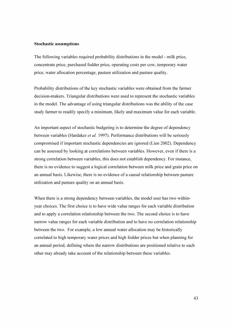
43

Stochastic assumptions

The following variables required probability distributions in the model - milk price,

concentrate price, purchased fodder price, operating costs per cow, temporary water

price, water allocation percentage, pasture utilization and pasture quality.

Probability distributions of the key stochastic variables were obtained from the farmer

decision-makers. Triangular distributions were used to represent the stochastic variables

in the model. The advantage of using triangular distributions was the ability of the case

study farmer to readily specify a minimum, likely and maximum value for each variable.

An important aspect of stochastic budgeting is to determine the degree of dependency

between variables (Hardaker et al. 1997). Performance distributions will be seriously

compromised if important stochastic dependencies are ignored (Lien 2002). Dependency

can be assessed by looking at correlations between variables. However, even if there is a

strong correlation between variables, this does not establish dependency. For instance,

there is no evidence to suggest a logical correlation between milk price and grain price on

an annual basis. Likewise, there is no evidence of a causal relationship between pasture

utilization and pasture quality on an annual basis.

When there is a strong dependency between variables, the model user has two within-

year choices. The first choice is to have wide value ranges for each variable distribution

and to apply a correlation relationship between the two. The second choice is to have

narrow value ranges for each variable distribution and to have no correlation relationship

between the two. For example, a low annual water allocation may be historically

correlated to high temporary water prices and high fodder prices but when planning for

an annual period, defining where the narrow distributions are positioned relative to each

other may already take account of the relationship between these variables.

44

Narrow distributions imply that the seasonal forecast is relatively accurate compared to a

longer term multiple-year forecast. Only if the forecast year is completely unknown

should correlations be used with wide variable distribution ranges.

In the current case study modelling, where forecasts were single year rather than multiple

year, narrow variable ranges were selected and no programmatic correlations were

applied to stochastic variables in the Monte Carlo simulations.

3.5 Data collection

Data collection for the case studies involved a two step process, the first a personal on-

farm interview and the second the gathering of prior year and projected year physical and

financial data.

3.5.1 Case study farm interview

A recorded personal interview took place with each of the respective farming couples in

the case studies. Their views, opinions and approaches on the following matters were

sought:

a) Technical, production and husbandry issues. b) Financial and debt-servicing issues. c) People and decision-making issues. Each was asked to describe how they had managed their farming system within the last 5

years. This particular period involved a range of extreme climatic events, high input

costs, abnormally high milk prices, and an unusual milk price collapse. To assist the

farmers in their recollection of events, a set of backup prompting questions (Appendix 1)

was developed for use when the farmers failed to provide sufficient detail or had

neglected to cover an important subject matter area. The questions covered the

background detail of how each farmer responded to previous events and their degree of

success in responding to the risks during this period.

45

An audio transcript of the two interviews was produced to provide a reference on the

choice of decisions that were to be made in the analysis. The transcript also allowed

personal observations about their farm system, external events, risk and decision making.

3.5.2 Farm performance data

Comprehensive physical and financial data were collected from the case study farms for

the 2010-11 year. Physical data included land areas, livestock numbers, purchased and

consumed concentrates, fodder and other feeds offered to the dairy herd, milk production

details, cow live-weight, irrigation water use and ownership of high and low reliability

water right.

Financial data collected of the 2010-11 season included net milk income, livestock

income, other farm income, all fixed and variable operating costs, finance costs,

temporary water purchases and capital purchases or sales.

3.6 Description of scenario testing

3.6.1 Defining each years season forecast

For each of the six years for the analysis, price levels between years was set for the

following commodities - milk price, concentrate price, purchased fodder price, temporary

water price. Climatic variability was accounted for through water allocation and by

varying water use efficiency expressed as tonnes of pasture DM utilized per megalitre of

irrigation water. The season forecasts for each of the six years were designed with

consultation of the two case study farmers.

Both case study farms had to plan for the same seasonal forecast and undergo the same

external conditions in each year. Price differences for milk and concentrates were

allowed between the two farms. The domestic milk factory supplier achieved a 33 c per

46

kgMS premium over the export milk manufacturing supplier, and price of purchased

concentrates was varied, depending on nutritional quality and on whether grain was

processed on-farm by the farmer or off-farm through a commercial stockfeed supplier.

3.6.2 Defining each scenario

For each year and associated forecast of season and price, several alternative planning

options were defined for each case study farm. Based on the farmer interviews, the first

planning option (designated Option 1 or Control in the results) described what the farmer

would most likely do when faced with that particular set of forecasts. The farms are

operated in the model in a manner in which the researcher believes how the farmer would

have responded, knowing their farm and system. Other planning options tested the

financial merit of alternative decisions.

3.6.3 Stochastic simulation

For each of the management options available in year 1 to each case study farm, a

stochastic simulation was conducted to determine the most favourable decision option

based on growth in equity and net cash flow after tax. Once the most favourable decision

option for year 1 was determined, all bar one of the management options for the

subsequent year proceeded from and were linked to the financial outcome of that most

favourable planning scenario (see Figure 3-1). The exception was Option 1 in each year

which always proceeded from and was linked to the Option 1 financial outcome of the

previous year. The stochastic simulation process was repeated individually for each year

thereafter until year 6. This process is shown diagrammatically in Figure 3-1,

representing 3 of the 6 years modelled.

47

Figure 3-1 Description of the method of how the management options were assessed (Red line is the

Control pathway whereby Option 1 was selected every year and the Blue line is the Optimal pathway

whereby the most favourable option was chosen every year. All outcomes in the following years for

each pathway were derived from the chosen precedent options.

In addition to the above, two additional strategic options were tested for case study farm

1 in year 1, the first option being the sale of 500 megalitre of high security water right

and the second option being the sale of 500 megalitres of high security water right with

the purchase of 500 megalitres of low security water right. These options were not

explored for case study farm 2 because the farmers were adamant that they would never

sell high security water right.

3.6.4 Comparison of cumulative farm plans

Once all scenarios were tested for each of the six years, two alternative planning

pathways were described, one the ‘control’ plan pathway and the other the ‘optimal’ plan

pathway. The ‘control’ plan pathway represented the cumulative outcome resulting from

the decision maker selecting all of the option 1 choices in each year. The ‘optimal’ plan

pathway represented the cumulative outcome resulting from the decision maker selecting

the most favourable option in each year.

Option 1

Option 2

Option 3 Favourable

Option 4 Option 4

Option 3

Option 2 Favourable

Option 1

Option 4 Favourable

Option 3

Option 2

Option 1

Year 1 Year 2 Year 3

Previous (Base) Year

Outcome

Control

Pathway

Optimal

Pathway

48

For each of the two case study farms, the two planning pathways were compared by

conducting a stochastic simulation, measuring the six year cumulative discounted growth

in equity and return on assets managed for each year and determining the aggregate

financial merit of each pathway for each farm.

Subsequently, for each of the two case study farms, the two optimum planning pathways

were compared by determining return on assets managed in each year.

3.7 Summary of method

To examine the investigation on the production and financial outcomes that arise from a

multi-year sequence of tactical farm management decisions in two case study irrigated

dairy farms in Northern Victoria, the in-depth case study approach was adopted. The

approach to analysing the two case study farms integrates Yins (1989) four tests of logic

for assessing case studies. The case study profiles designed were a ‘medium’ input farm

and a ‘high’ input farm.

A biophysical and economic performance analysis performed over a six year period of

varying climatic and economic conditions was used to analyse each case study farms

tactical farm management decision options. The measures to assess the effect on each

case study farm of the experimental decisions taken were annual growth in equity, net

cash flow after tax, cumulative discounted growth in equity and return on assets

managed.

The next chapter presents the analysis of case study Farm 1 ‘medium’ input and is

repeated in Chapter five for case study Farm 2 “high” input. A comparison of the two

case studies is documented in Chapter six.

49

4 Case study 1 – Medium input farm

4.1 Description of Farm 1

Located in the Stanhope region in northern Victoria, Farm 1’s a “medium” input farm

with a herd size of 300 cows supplying an export milk manufacturing company. The

business is a family run farming enterprise, with management and labour supplied by the

husband (50 hrs a week). There is a full time labour unit (50 hrs a week) and a part time

labour unit (48 hrs a week for 24 weeks) employed. The home farm is comprised of 263

ha, of which 230 ha is available for pasture or cropping production, and of that area, 90

ha is available for the milking herd.

Farmer 1 comments:

“We’re milking about 300; we’d probably like to get to about 320 over the next year or two unless the property is expanded of course. Because of the extended lactation, we’re now getting more replacements than we need, so we will have heifers probably for sale.”

“Pre-drought we were all perennials - 90 hectares of perennial pasture and no annuals. As a result of the drought, we certainly changed the mix, although we still consider perennial pastures important to our business. At the moment, we’re still at 60 hectares of perennials and 30 hectares of annuals - we’re fairly comfortable with that. Even with the increased water availability, the two third – one third mix seems to suite us.”

In the 2010-11 season, the farm had a calculated pasture utilization of 12.65 tDM per ha

on the milking area, representing 2.74 tDM pasture grazed per cow. There was 317 tDM

of home grown fodder cut and 153 tDM of fodder purchased. In the dairy, 1.66 tDM of

straight triticale, rolled on-farm and without mineral or protein supplementation was fed

per cow.

“We obviously like to get as much grass as we can into them. It’s been difficult over the last few years, with locusts last year and very dry seasons previously. Feeding up to 1.8 tonnes prior to this year - just triticale in the bale - with some supplementary fodder fed in the paddock when required. Up to this year, the strategies haven’t changed, just the quantities. We eventually put in a “feed pad” (actually a Waste-Not feeder) during the drought to stop wastage, which we still use every now and again.”

“We grow the majority of our own fodder crops, we buy some milking quality hay but the majority we grow. It’s a mix, some cereals and some annual pastures. There was very little

50

grown in the droughts. We’ve got a runoff block - usually we cut the cereals out there and we cut the annuals here at home.” “We’re pretty well self-contained for heifer rearing. Calves are all reared here (at home), we’ve got a runoff block so they stay here usually till they are 12 months old, then go to the runoff block till they’re ready to calve.”

The majority of the farm’s soils consist of Shepparton fine sandy loam.

“We soil test regularly - sort of a rolling 3 year average - so that each paddock would get tested every 3 years and we apply fertilizer accordingly. We don’t aim for the sort of levels we did with an Olsen P as a few years ago. We’ve been in mining maintenance phase since the drought started. So as long as the Olsen P is over 20, we’re comfortable”.

The fertilizer program for 2010-11 consisted of 32 t superphosphate, 23 t urea, 8 t liquid

N and 3 t DAP, across the home farm and runoff block.

The farm has 739 megalitres of high security water right supplied from the Goulburn

irrigation system. In 2010-11, 365 ML of irrigation water was used, producing a water

use efficiency of 2.25 tDM of pasture utilized per ML. The season had above average

rainfall, so less irrigation was required.

A full description of the production and economic performance of the farm business for

the 2010-11 season (labelled ‘Previous Year’ in tables) is in Appendix 2. In summary, the

farm produced 1,628,430 litres of milk, 70,609 kg of fat (4.34 %) and 57,994 kg of

protein (3.56 %). The herd on average produced 5428 litres per cow.

Financially, the business had a good year in 2010-11 with a growth in equity of $164,347

that increased the owner’s equity percentage from 65 % to 68 %. A return on assets

managed of 7.43 % and a return on equity of 14.11 % was achieved. The return on asset

compared very similar to the average achieved from the 24 farms in the 2010-11 dairy

industry farm monitor project in Northern Victoria (Department of Primary Industries

2011) with an average return on asset of 7.0 % and average return on equity of 7.6 %.

Although the farm had a net cash flow before tax of $113,970, there was a contribution of

51

$145,242 from milk factory share sales, so net cash flow would have been negative if the

factory shares were not sold.

A full detailed description of the physicals and financials of Farm 1 for the 2010-11 year

can be found in Appendix 2.

4.2 Year 1 Farm 1 analysis

4.2.1 Year 1 season forecast settings

In Year 1, there is a reduction in milk price from $5.43 in 2010-11 to $4.85 per kgMS.

Concentrate price per tonne increases $30 t to $250 and purchased fodder is estimated to

be at $140 t DM. There is a very high chance of 100 % water allocation with temporary

water price expected to be around $25 ML. There is 525 ML of water carried over from

the previous season.

4.2.2 Year 1 options available

Option 1: Continue farming the same way as in the 2010-11 year with a herd size of 300,

feeding 1.77 t DM of triticale per cow, achieving slightly more pasture grazed per cow at

3.0 t DM and feeding 260 t DM of home grown fodder and 231 t of purchased fodder.

Milk yield is in the high 5,000 litres per cow.

Option 2: Increase herd size from 300 to 320, reduce home grown fodder from 260 t to

240 t to increase pasture consumption, recognising that pasture grazed per cow decreases

to around 2.9 t DM with the extra cows. Stocking rate has now increased from 3.33 cows

per hectare to 3.67 cows per hectare from baseline levels.

Option 3: Option 2 repeated with an increase in grain quality by replacing straight

triticale with a commercial grain mix that contains a blend of wheat and proteins and

minerals. This change is represented in the model with a 0.8 MJ ME per kgDM increase

52

in feed quality for concentrates for a $110 per tDM price premium. Milk yield per cow

lies in the mid 6,000 litres.

4.2.3 Year 1 Farm 1 results and discussion

Figure 4-1 Growth in equity of three alternative options for Year 1 Farm 1

Option 2 was the most favourable option for increasing growth in equity, with a mean

growth of $65,070 (st dev $24,960) compared to Option 1 $55,292 (st dev $23,103) and

Option 3 $52,190 (st dev $25,892). The decrease in livestock sales in Option 2 and 3 to

increase herd size will make the year difficult with cash flow, with a projected net cash

flow after tax of -$33,217 for Option 2 and -$46,097 for Option 3, compared to -$16,843

for Option 1.

Option 1 set a herd size of 300 cows since there was a 10 % decrease in milk price from

2010-11 to Year 1. Option 2 tested the farmer’s strategy of growing the herd size to

around 320 cows in the future. The higher stocking rate turned out to be the most

favourable option in terms of growth in equity. The choice between Option 1 and Option

2 was a difficult one due to the losses in cash flow involved in each, however Option 2

53

was chosen as it had potential to take advantage of a favourable proceeding season should

it occur. For Option 3, paying a premium of $110 tDM for a mixed blend of concentrates

under Year 1 circumstances and at the specified feeding rate was not as profitable as the

existing method of feeding home-milled triticale on farm.



In Year 2, the milk price is projected to decrease another 1 % to $4.80 per kgMS. A drier

season is forecast with cereal grain prices expected to increase $100 tDM to $350 tDM,

purchased fodder forecast to be up $60 tDM to $200 tDM, water allocation likely to be at

90 % and temporary water price at $90 ML. There is 600 ML of water carried over from



Option 1: Continuing on from Option 1 in Year 1, herd size increases from 300 to 310

cows. The same feeding strategy as Option 1 in Year 1 is repeated.

Option 2: Continuing on from Option 2 in Year 1, herd size is maintained at 330 cows

and the same feeding strategy as Option 2 in Year 1 is repeated.

Option 3: Continuing on from Option 2 in Year 1, herd size is reduced to 310 cows by

selling an additional 20 cows. The feeding strategy adopted is the same as in Option 1.

54

4.3.3 Year 2 Farm 1 results


Option 1 had the smallest mean decrease in equity growth of -$7,489 (st dev $26192)

compared to Option 2 -$16,225 (st dev $27,328) and Option 3 -$21,151 (st dev $26,190).

Option 3 was chosen as the preferred strategy over Option 2 since it had the most

favourable net cash flow, despite it having the greatest loss in equity growth. Option 3

had a net cash loss of -$54,679 compared to Option 1 at -$67,017 and Option 2 at -

$75,753 and.

Option 1 would have been the preferred option to choose in this season however because

options 2 and 3 were starting from a different pathway to Option 1, the choice had to be

out of those two. In a poor financial season such as is specified, choosing between an

option that has $21,074 more cash flow will be more favourable than an option that has a

greater gain in equity of $4,926, so Option 3 was selected and the herd size was reduced

to 310 cows.

55



In Year 3, a drought has a significant effect on commodity supply and price. Water

allocation is reduced to a likely 30 % allocation, temporary water price increases to $300

per ML, cereal grains increase to $420 per tDM and purchased fodder increases to $330

per tDM. Milk price improves slightly to $5.05 per kgMS. There is 600 ML of water

carried over from the previous season.


Option 1: Continuing on from Option 1 in Year 2, herd size is reduced from 310 to 280,

pasture utilization is reduced from 12.8 tDM per hectare to 9.0 tDM per hectare, pasture

grazed per cow reduces to 2.5 tDM per cow and the herd is supplemented with more

purchased fodder. Milk yield is around 5700 litres per cow.

Option 2: Continuing on from Option 3 in Year 2, herd size is maintained at 310 cows,

pasture utilization is reduced to 9.0 tDM per hectare, pasture grazed per cow reduces to

2.3 tDM, and the herd is supplemented with more triticale and purchased fodder.

Option 3: Continuing on from Option 3 in Year 2 but applying the same strategy as

Option 1.

Option 4: Continuing on from Option 3 in Year 2 with the same strategy as Option 3

except for a reduction in concentrate feeding of 0.35 tDM per cow. Milk yield is reduced

to around 5300 litres per cow.

Option 5: Continuing on from Option 3 in Year 2 with the same strategy as Option 3 but

with triticale replaced with commercial concentrates that contain a wheat and protein

blend, concentrate quantity increased by 0.35 tDM per cow, concentrate quality increased

by 0.8 MJ ME and concentrate cost increased by $110 tDM. Milk yield is increased to

6,800 litres per cow.

56


Figure 4-3 Growth in equity of five alternative options for Year 3 Farm 1

Option 5 was the most favourable option with an expected mean loss in equity of -

$114,346 (st dev $26,449) and cash loss of -$167,187 compared to Option 3, which had a

mean loss in equity of -$120,041 (st dev $25,421) and cash loss of -$172,887. Options 2

and 4 had the greatest loss in equity at -$146,173 (st dev $26,844) and -$148,570 (st dev

$24,990) respectively. Option 1 had a mean loss in equity of -$116,721 (st dev 25,434)

and cash loss of -$169,567.

Clearly the modelled drought had a significant negative impact on farmer 1’s planning

strategies. When asked about planning strategies for his next drought, the farmer

responded:

“We would probably retain a fair percentage of perennials, even though they weren’t brilliant in a true sense, because they were not irrigated through the whole season. We found if we can get them through to Christmas, then there is still a fair percentage of ryegrass still alive come autumn. And obviously if your water supply is limited then you use it in the spring and autumn where there is a bigger bang for your buck.”

57

The farmers strategy not to irrigate through the whole season was reflected in all tested

options in Year 3 with the decrease in pasture utilization from 12.8 tDM per hectare to 9

tDM per hectare. Reflecting this reduced irrigation, water use efficiency in the modelling

was increased from 1.65 tDM per ML to 1.9 tDM perML, to account for the better

irrigated pasture yields per megalitre when only Spring and Autumn are considered.

When asked about stocking rate in previous droughts, the farmer replied:

“(Stocking rate) Pretty much stayed around the same, we did cut back a bit during the drought. On average milking around 320 cows, we probably got down to about 270 in a couple of the really tough years. We took the view that it was easy to bounce back if we had a reasonable number of cows carried through.”

The modelling demonstrated that cutting back the herd size, shown in Options 1, 3 and 5,

was more profitable than trying to maintain herd size as shown in Option 2.

The modelled Options 1, 3 and 5 probably underestimate real world profitability. In the

model, all cows are treated as an average cow, each with the same production efficiency,

so when herd size is reduced as a drought strategy, the model ignores efficiency

differences between cows. In reality, when farmers cut herd size back, they sell their least

efficient cows, leaving a more efficient herd with increased average production.

Option 5 was the most favourable outcome due to the increase in supplement spending on

quality and quantity, to increase cow production. Growth in equity differed by $34,224

between this option and Option 4, where there was a decrease in supplement spending

and a consequent reduction in cow milk production.



In Year 4, the drought continues although it is not as severe as in Year 3. Cereal grain

prices ease to $370 t DM, purchased fodder price falls to $280 tDM and water availability

increases to a likely 40 % allocation. Temporary water price decreases to $250 per ML,

58

milk price increases to $5.53 per kgMS and there is 350 ML of carry over water available

from the previous season.


Option 1: Continuing on from Option 1 in Year 3, herd size is increased from 280 cows

to 300 cows. The same feeding strategy as in Option 1 in Year 3 is adopted, with slightly

more purchased fodder and triticale per cow to supplement the larger herd. Pasture

utilization is kept at 9 tDM per ha, despite the higher stocking rate.

Option 2: Continuing on from Option 5 in Year 3, the same feeding strategy as Option 1

is used.

Option 3: Continuing on from Option 5 in Year 3, herd size is reduce herd size from 280

cows to 260 cows, pasture utilization is kept at 9 tDM per ha, grazed pasture per cow lifts

to 2.7 tDM, allowing a decrease in quantity of triticale and purchased fodder fed per cow.

Milk yield per cow is around the high 5000 litres.

Option 4: Continuing on from Option 5 in Year 3, herd size is reduced from 280 cows to

260 cows and triticale is replaced with a commercial wheat and protein concentrate.

Concentrate price increases by $110 tDM, the quantity of concentrates fed is lifted to 2.3

tDM per cow and milk yield lifts to the low 7000 litres per cow.

Option 5: Continuing on from Option 5 in Year 3, herd size is increased to 300 cows and

pasture utilization is increased from 9 tDM per hectare to 12 tDM per hectare by

irrigating through the summer. For this summer irrigation, the last 3 tonnes of pasture

yield per hectare has a marginal return of 1 t DM per 1 ML of water. Pasture grazed per

cow is lifted to 3.1 tDM, triticale is reduced to 1.5 tDM percow and milk yield lies

around 6,000 litres per cow.

59

Option 6: Continuing on from Option 5 in Year 3, herd size is increased to 300 cows,

pasture utilization is lifted to 12 tDM per hectare and a commercial wheat protein

concentrate fed at a rate of around 2 tDM per cow. Milk yield is around 7,000 litres per

cow.


Figure 4-4 Growth in equity of five alternative options for Year 4 Farm 1

Option 6 had the smallest decrease in equity of -$80,873 (st dev $26,189) compared to

Option 4 at -$89,657 (st dev 24,975), Option 5 at -$100,904 (st dev $26,790), Option 1 at

-$110,568 (st dev $26,189), Option 2 at -$114,615 (st dev $26,408), and Option 3 at -

$115,163 (st dev $23,788).

Although Option 6 had the smallest loss in equity, Option 4 had the smallest net cash

deficit after tax of -$25,229, compared to Option 6 at -$68,445. This cash difference can

be attributed to differences in livestock sales since Option 4 reduces herd size and Option

6 increases herd size. Option 4 resulted in lowered non-supplement operating costs

($363,722) while Option 6 resulted in increased non-supplement operating costs

60

($399,900). However, on a per cow basis, Option 6 decreased to $1,333 and Option 4

increased to $1,398.

Selecting the preferred choice between Options 4 and 6 is difficult since there is a herd

size difference of forty cows and the selection would be influenced by limits to cash flow.

The projected equity percentage at the start of Year 4 is a sound 66 %, so the business

would be able to get loan funds to undertake Option 6. Option 6 was preferred over

Option 4 since it allowed the business to be better set up for the following year, should

favourable market and climatic conditions occur.

In Year 4, there is reward in spending greater cash on concentrates and or purchased

water as shown in the results for Options 4, 5 and 6. Based on growth in equity, the

decision maker would be indifferent between Option 2 where the herd size is increased

and Option 3 where the herd size and production per cow is reduced. However, there is a

large difference in net cash flow after tax for Option 2 (-$102,187) and for Option 3 (-

$50,735). Therefore if the decision maker chose not to spend cash on extra feed and

water (Options 4, 5 and 6), he would likely opt for the Option 3 strategy.



Year 5 is a recovery year after the drought, with water allocations increasing to a likely

80 % allocation, temporary water price decreasing to $50 ML, cereal grain prices

decreasing to $300 per tDM, purchased fodder prices likely to be $180 per tDM and milk

price increasing to $5.88 per kgMS. There is 160 ML of carry over water available from



Option 1: Continuing on from Option 1 in Year 4, herd size is held at 300 cows, pasture

utilization is increased to 12.8 tDM per hectare, grazed pasture per cow increases to 3.07

tDM, 1.6 tDM concentrates (triticale) is fed and milk yield lies near 5,900 litres per cow.

61

Option 2: Continuing on from Option 6 in Year 4, herd size increases from 300 cows to

330 cows. Pasture utilization increases to 12.8 tDM per hectare, grazed pasture per cow is

2.88 tDM, concentrates are fed at the rate of 1.66 tDM per cow and milk yield lies near

5,850 litres per cow.

Option 3: Continuing on from Option 6 in Year 4, herd size increases from 300 cows to

330 cows and triticale is replaced with a commercial wheat protein concentrate, at an

increased rate of 2.0 tDM per cow and at an additional cost of $110 per tDM. Milk yield

lies near to 6,800 litres per cow.



Option 3 had the highest growth in equity of $144,335 (st dev $30,332) and highest net

cash flow after tax of $107,924. Option 2 had the second highest growth in equity of

$115,649 (st dev $29,249) but a smaller net cash flow after tax of $79,231. Option 1 had

a net cash flow after tax of $94,263 and growth in equity of $104,674 (st dev 28,006).

62

For Year 5, it was beneficial to be marginally overstocked in respect of grazed pasture

per cow since there was reward for increasing production per cow through concentrates.

In the modelled sequence of years, Year 5 is the first year out of drought and the first

year for this farm to take advantage of a favourable season after several poor years of

economic returns. The decisions made in these ‘safe’ seasons still have a big impact on

the long term profitability and survival of the business. All options assumed that the farm

would produce the same volume of pasture as before the drought. In reality, if the

decision maker failed to get pasture production back on track immediately after the

drought, it is likely that there would be continuing poor returns for the year after the

drought.



In Year 6, the recovery continues with favourable seasonal conditions. Water allocation is

a likely 100 % allocation, temporary water price is at $25 per ML, cereal grain prices

decrease to $210 per tDM, purchased fodder price is $180 per tDM and milk price has

increased to $6.00 kgMS. There is 200 ML of carry over water available from the

previous season.


Option 1: Continuing on from Option 1 in Year 5, herd size is held at 300 cows. Pasture

utilization is 12.8 tDM per ha and grazed pasture per cow is 3.0 tDM. Purchased fodder is

fed at 1.0 tDM per cow, home grown fodder is fed at 0.63 tDM per cow and triticale is

fed at 1.7 tDM per cow. Milk yield lies near 6,000 litres per cow.

Option 2: Continuing on from Option 3 in Year 5, herd size is held at 330 cows. Pasture

utilization is 12.8 tDM per hectare and grazed pasture per cow is 2.9 tDM. Purchased

fodder per cow and home grown fodder per cow are 1.1 tDM and 0.61 tDM respectively.

63

A commercial wheat and protein concentrate mix is fed at 1.75 tDM per cow at a $110

tDM price premium. Milk yield lies near 6,300 litres per cow.

Option 3: Continuing on from Option 3 in Year 5, herd size is increased from 330 cows

to 345. Pasture utilization is 12.8 tDM per hectare, grazed pasture per cow is slightly

lower than Option 2 at 2.9 tDM, purchased fodder is fed at the rate of 1.25 tDM per cow,

home grown fodder is fed at 0.45 tDM per cow and 1.75 tDM of triticale is fed per cow.

Milk yield is near 6,000 litres per cow.

Option 4: Continuing on from Option 3 in Year 5, with Option 3 repeated, but with

triticale replaced with a commercial wheat and protein concentrate which was fed at the

higher rate of 2.0 tDM concentrate per cow. Milk yield approaches 6,900 litres per cow.


Figure 4-6 Growth in equity of four alternative options for Year 6 Farm 1

Option 4 was the most favourable option with a mean growth in equity of $284,308 (st

dev $31,432) and net cash flow after tax of $237,550, compared to Option 3 with a

64

growth in equity of $253,491 (st dev $30,449) and net cash flow after tax of $206,733.

Option 2 had a growth in equity of $193,871 (st dev $29,238) and net cash flow after tax

of $166,613 and Option 1 had mean growth in equity of $223,403 (st dev $28,308) and

net cash flow after tax of $183,145.

The results show that in a favourable season, it is important to be responsive tactically,

considering the large differences in outcomes between options, compared to previous

years. Option 4 had a growth in equity $90,437 greater than that of Option 2. Both

Options 4 and 2 increased the quality of concentrates fed and Option 4 also increased the

amount of concentrates fed to 2 tDM per cow. Combined with an increase in herd size,

Option 4 produced greater milk production per cow and higher milk revenue, while

maintaining good grazed pasture per cow levels, with a reduction in the amount of home

grown fodder able to be conserved. However, the downside of Option 4 is that there is a

lower strategic fodder reserve available for the future and potentially an increased

reliance on purchased fodder.

4.8 Six year cumulative effect of decision making on Farm 1

Over the six years tested, there are now two pathways - a ‘control’ pathway which

combines all of the Option 1’s in each year and the ‘optimal’ pathway which combines

the most favourable decision option chosen in each year.

4.8.1 Six year cumulative Results for Farm 1

Appendix 2 provides the full six year physical and financial outcomes of the ‘control’ and

‘optimal’ pathways for case study Farm 1, showing the combined impact over the full

period of tactical decisions taken in each year. It must be noted however the results in the

Appendix are static results, not simulated, so all the physical and financial detail can be

represented. As a result static values will be slightly different to the simulated values

represented in Figure 4-7 and Table 4-1. Figure 4-7 shows the simulated six year

cumulative discounted growth in equity of the two pathways. The ‘control’ pathway had

65

a cumulative discounted growth in equity of $90,060 (st dev $61,677) while the ‘optimal’

pathway had a more favourable cumulative discounted growth in equity $190,301 (st dev

$64,663). The annual return on assets managed for the ‘control’ and ‘optimal’ pathways

is shown in Table 4-1. Year 2 was the only year where the ‘control’ had a greater return

on assets managed compared to the ‘optimal’ pathway.

Figure 4-7 Six year cumulative discounted growth in equity of ‘control’ and ‘optimal’ pathways for

Farm 1 (Medium input)

66

Table 4-1 Return on assets managed for ‘control’ and ‘optimal’ pathways

Figure 4-7 and Table 4-1 show the cumulative effect that fine tuning of tactical decisions

can have on long term profitability and wealth creation. The ‘optimal’ pathway had a

growth in equity mean of $100,241 greater than that of the ‘control’ pathway. However,

this value difference is not the difference between Farm 1’s worst possible outcomes and

its best possible outcomes. The ‘control’ pathway is limited to the assumptions derived

from the farmer’s answers at interview on what they would do under various

circumstances. The ‘optimum’ pathway is a result of testing particular tactical strategies

to determine the most favourable pathway financially. So to achieve a mean equity

difference of $100,241 between the two pathways, simply by making minor changes to

the farming system, may be quite significant. In the farm case study interview, Farmer 1

was asked about his views on targeted milk production in the context of an annual farm

plan. The farmer replied:

“I guess in the past we haven’t been driven by production, that’s probably an area that we’re looking at the moment, it’s probably a result of your visit last year. We’ve gone to feeding a mixed ration (commercial concentrates mix). We didn’t start quite as early as we’d planned for one reason or another, but have been really encouraged by the results. It’s probably just a matter of deciding how far we take that change.”

Year 1 2 3 4 5 6

Control ROA 5.22% 3.03% -0.14% 0.28% 7.33% 10.59%

St dev 0.61% 0.65% 0.70% 0.77% 0.77% 0.79%

Optimal ROA 5.67% 2.83% 0.02% 1.29% 8.67% 12.26%

St dev 0.65% 0.66% 0.74% 0.77% 0.84% 0.86%

Control ROE 3.62% 0.17% -5.14% -5.28% 5.17% 10.40%

Optimal ROE 4.06% -0.36% -5.20% -3.95% 7.14% 12.97%

Control growth in equity $55,292 -$7,489 -$116,721 -$110,568 $104,674 $223,403

Optimal growth in equity $65,070 -$21,151 -$114,346 -$80,873 $144,335 $284,308

Control cumulative discounted

growth in equity $90,060

St dev $61,677

Coefficient of variation 68.48%

Control cumulative equity growth as a percentage of starting equity 3.61%

Optimal cumulative discounted

growth in equity $190,301

St dev $64,663


Optimal cumulative equity growth as a percentage of starting equity 7.64%

67

The advantage with changing tactical approaches is that they are reversible, unlike most

strategic decisions. If a farmer feels that the stocking rate is set too high, it can easily be

reduced. Nutritional strategies can be immediately changed depending on either

favourable or unfavourable movements in market and or climatic conditions.

The results suggest that there is merit in assessing decision options on an annual basis

since decisions taken and market and climatic circumstances in each unique year always

result in different financial outcomes. What may have been a favourable plan in one year

with a certain set of climatic and market values may not be the most favourable plan in

other years with different climatic and market values.

A recent Dairy Australia study found that most of the dairy farmers in the study did not

change their pasture, fodder or concentrate intakes significantly over the 3 year study

period, despite large differences in milk, grain and fodder prices between those years

(Dairy Australia 2011b). Given the difference in equity generated by the two pathways

described above, based on reasonable scenario testing, efforts to improve the annual

planning process used by dairy farmers may prove very worthwhile.

Change in discretionary spending between years was not included in the analysis.

Discretionary spending was held constant throughout the six year model period to allow a

better gauge of the effect of the other measures. The reality on Farm 1 was different to

the modelled outcomes. When asked about cash flow management in the dry years, the

farmer replied:

“Nothing specific, where you could avoid spending money you did, although we were committed to developing the farm. We cut down labour costs and trimmed anything we could with the discretionary spending.”

68

4.9 Alternative Strategic option – Sell high security water

A common dilemma for farmers in Northern Victoria over recent years is whether to keep

their high security water right or to sell it. When asked about the future of irrigation in the

region, Farmer 1 replied:

“I’m still quite positive about it, there are certain questions to whether it pays to own permanent water entitlement, or just go into the temporary water market. We recently just sold a couple of hundred megalitres. Given the amount of land that’s gone out of production to dairying, we’re of the view that it (water) will still be adequate, unless it’s in the really tough years.”

To assess the merit of farmer 1 selling his high security water right, his two pathways

described above were re-run. In the re-run, 500 ML of high security water share was sold

in Year 1 to reduce existing farm debt. Subsequently, the same tactical decisions were

made for each year and any shortfalls in water allocation were purchased from the

temporary water market. A second option looked at the scenario where 500 ML of high

security water was sold in Year 1 in the optimal pathway and 500 ML of low security

water right was purchased to retain the same amount of carry over water.

69

4.9.1 Sell high security water results

Figure 4-8 Six year cumulative discounted growth in equity for control and optimal pathways with

and without the sale of 500 ML of high security water right and with and without the purchase of low

security water right in Year 1

Selling 500 ML of high security water right had favourable effects on both the control

pathway and optimal pathway. When the high security water was sold, the control

pathway increased from a mean six year cumulative discounted growth in equity of

$96,437 (st dev $59,630) to $140,244 (st dev $59,180), an improvement of $43,807 and

the optimal pathway increased from a mean $197,008 (st dev $63,159) to $253,146 (st

dev $60,875), an improvement of $56,138. When in the optimal pathway 500 ML of low

security water right was purchased after selling 500 ML of high security water right in

Year 1, the mean six year cumulative discounted growth in equity increased to $280,847

(st dev $58,543).

The sale of 500 ML of high security water right at $1500 per ML allowed the business to

reduce principal and interest payments, freeing up cash flow. This would assist the farmer

to source water from the temporary water market. Another option that could have been

70

assessed following the sale of the water was expanding the business in size and scale.

However, the farmer was uncertain about where the business was heading in terms of

succession, so this option was not examined.

The purchase of the low security water was even more profitable than selling high

security water right on its own as it allowed the business to safely carry more temporary

water over into the drought years, to ease the water burden in the drought and to reduce

the impact of year to year climatic volatility.

71

5 Case study 2 – High input farm

5.1 Description of Farm 2

Located in the Lockington region in Northern Victoria, Farm 2 is a “high” input farm

with a herd size of 700 cows supplying a domestic milk manufacturing company.

“We’re sitting on a herd size of about 700 now, we could probably milk 800 and we’ll probably get to 800 I think. If we equal our grass, then we’re at our maximum profitability, throwing in a bit of grain and hay if its still making us a quid in the margins, I don’t see a problem with that…but we do know, over the next 3 or 4 years we want to get somewhere around 800 and 900 cows, we want to run 2 herds, we want to have a herd manager in charge of each herd, we can do that on this farm.”

“My optimum stocking rate was always to have the farm stocked to the point where you didn’t cut any hay off where the cows grazed. You had enough cows to deal with the pasture in spring, and after that you filled the gap. That used to be 2 cows to the acre, 5 to the hectare. We’ve probably come back a fractionally from that because we’re growing a lot more feed and we haven’t quite got enough cows. We don’t go far away off that, that’s still basically our driver. We were certainly that in the nineties, we started with around 5 cows to the hectare with only grain and no feed pad, feeding out to a round bale with smaller numbers of cows. It gets a bit more difficult with big numbers of cows to run that rate, particularly milking cows through the winter. We would be a bit over 4 cows to the hectare now.”

The business is a family run farming enterprise, with management and labour supplied by

the husband and wife (90 hrs a week). There are 5 full time and 2 part time labour

personnel employed. The farm is comprised of 278 ha, of which 263 ha is milking area.

“Over the last 5 years we had a third of the farm in lucerne and the rest permanent pasture. There’s a small area down the back that doesn’t water too well with annuals. But over the last 2 years it’s all become either Lucerne or permanent pasture. I think in general terms we will keep a third of the farm in lucerne, but that will vary year to year depending on, and the rest of it will become permanent pasture. So there will be no annuals on the areas that the cows graze. And that’s been really beneficial last winter and before when it got really wet and the floods because we had somewhere to put the cows.”

“I didn’t cut any hay on the home farm this year milking 700 whereas last year milking 600 I did.”

In the 2010-11 season, the farm had a back calculated pasture utilization of 8.99 tDM per

hectare on the milking area, 3.35 tDM pasture grazed per cow. There was 222 tDM of

home grown fodder cut and 375 tDM of purchased fodder. In the dairy, 2.61 tDM of

72

concentrates were fed per cow. The concentrates of wheat, canola meal, lupins and

minerals are rolled and mixed on farm.

“we would use our production as a guide for supplementary feeding. We manage the grass then we fill the gaps. The cows tell us the story of how much gap we need to fill.”

“But we’ve kept it as a pretty simple system so we think machinery is a waste of money and we think that mixer wagons and big tractors are just money chewers, so we just put in a waste-not system which can be done with a small tractor and it doesn’t need any other stuff, and we can put that into the waste-not feeder and the cows come out of the dairy and we can feed them for whatever length of time we like with anything we like in that system.”

Soils and Fertiliser “We’ve got Olsen P’s over 30 and we use a bit of nitrogen, a fair bit of nitrogen actually. We’re lucky here that most of the farm is on a sandy loam, and that’s a huge benefit to us because the grass grows better As far as the super goes, then we do the odd soil test, not every year, not every paddock, but we do a lot of soil tests. We put somewhere between half a tonne and a tonne of super on a year, not on the areas we are feeding out a lot, not on the areas where we calve, not on the areas where we put effluent. We throw nitrogen out on paddocks as required, particularly in the spring and in the autumn as the rotations are going out. We like to put super out at this time of year (Autumn) too because its got extra sulphur in it which helps to stimulate soil bacteria and just gets things going, whereas after a summer of irrigating and nitrogen boosting it needs that bit of sulphur to give it that autumn kick start, particularly if you’re starting up annual pastures. When we got here, it was over 107 acres but the guy who ran it had been very keen on his super and so were we, and we did some soil tests with Olsen P’s around 50 or 60. So in the drought we were able to take bit of a breather with cash flow to not put any super out. We decided we could mine for a couple of years and use money to buy water. With an Olsen P of 60 we didn’t need to add any more especially when we dried large chunks of the farm off. Anything we would water we would make sure the Olsen P’s and the nitrogens would be right.”

The business is structured with a large amount of water with 1100 ML of high security

water right and 2000 ML of low security water right to protect themselves from future

droughts.

“So we’ve bought a heap of low security water so that we can carry over water. We’ve got a goal of that we can carry over 2 years worth of water at all times, so that if we went into another drought we’d have 2 years where we would be ahead of the pack.”

73

In 2010-11 the farm produced 5,063,101 litres of milk, 197,314 kg of fat (3.90 %), and

169,673 kg of protein (3.35%). The milking herd on average produced 7911 litres per

cow.

“They do about 320 kgs of fat a year, 8200 litres, somewhere like that, and I think it’s about 260 kgs of protein. Less last year because the locusts knocked us last year and the humidity knocked us last year. Last year was a bad year for cows. So we’ve just found it’s a good compromise for the position. When grain was really expensive we tried to chop them back but they just got lighter, they wanted to produce the same amount of milk and the just got lighter. I guess we farm to our own recipe of we know it works. I think 10,000 litres you do run into troubles with udders collapsing and you also run into trouble getting them into calf, then you run into trouble with mastitis because they’re absolutely busting. We could get them to 9,000 litres, we’ve done it, we don’t really want to do it though, it’s not the profitable, we don’t think, point to be.”

Financially the business had a very good year in 2010-11 with a growth in equity of

$419,616 to increase the equity percentage from 57% to 61%. A return on asset of 12.56

% was recorded and a return on equity of 33.78 %. The farm had a net cash flow before

tax of $291,932.

“so we’re trying to build a system that might not be the best on a figures basis but it gives us a lot of flexibility. For everything we hear and read, climate change is going to give us a variable world, a far more variable world than what we’re used to farming in so we need to try and be ready to capture anything that comes our way.”



In Year 1 in the analysis there is a reduction in milk price from $5.99 in 2010-11 to $5.18

per kgMS. Concentrates increase $30 t to $360, and purchased fodder is likely to be

around $140 per tDM. There is a very high chance of 100 % water allocation with

temporary water price expected to be around $25 ML. There is 3000 ML of water carried

over from the previous season.


74

Option 1: Increase herd size from 640 to 700 cows. Pasture utilization continues at 10

tDM per hectare from previous season, 3.3 tDM grazed pasture per cow, 2.5 tDM

concentrates, Milk yield 8200 litres per cow.

Option 2: Decrease herd size from 640 to 600 cows. Pasture utilization is 3.3 tDM grazed

pasture per cow and no purchased fodder required. Milk yield is around 8200 litres per

cow.

Option 3: Increase herd size from 640 to 700 cows, reduce concentrates to 2.0 tDM per

cow and milk yield to around 7200 litres per cow.



Option 1 had the greatest growth in equity at $465,069 (st dev $66,408) compared to

Option 3 $330,895 (st dev $65,218) and Option 2 $329,965 (st dev $58,176). Option 1

also had the highest net cash flow after tax of $312,371, compared to Option 2 $310,044

and Option 3 $177,881.

75

Option 1 was the selected strategy in Year 1 where the herd size was increased and

production per cow was maintained. Option 2 underutilizes the farm resources and

Option 3 saved costs in supplements however the reduction in milk income was greater

than the savings.



In Year 2 the milk price is projected to decrease 1 % to $5.13 per kgMS. A drier season is

forecast with concentrate prices expected to increase $100 to $460 per tDM, purchased

fodder increases $60 to $200 per tDM, water allocation decreases to a likely 90 %

allocation and temporary water price increases to $90 ML. There is 3000 ML of water

carried over from the previous season.


Option 1: Continuing on from Option 1 in Year 1: Herd size is increased from 700 cows to 800 cows, all pasture grown on home farm is now grazed at 3.29 tDM per cow. Option 2: Continuing on from Option 1 in Year 1: Herd size is maintained at 700 cows and the same feeding strategy as Option 1 Year 1 is repeated.


76

Figure 5-2 Growth in equity of two alternative options for Year 2 Farm 2

Option 1 was the preferred method with a growth in equity of $381,544 (st dev $76,330)

compared to Option 2 with a growth in equity of $286,359 (st dev $69,951). Net cash

flow after tax was the only downside to Option 1 with $78,675 compared to Option 2 of

$145,475.

Option 1 has just reached a herd size where all the pasture grown on the milking area is

fully utilized by grazing at 10 tDM per hectare.



A drought takes full impact on commodities and their prices in Year 3. Water allocation

is reduced to a likely 30 % allocation, temporary water price increases to $300 ML,

concentrates increase to $530 tDM, purchased fodder increases to $330 tDM. Milk price

improves to a likely $5.36. There is 3000 ML of water carried over from the previous

season.

77


Option 1: Continuing on from Option 1 in Year 2: Pasture utilization is reduced from 10

tDM per ha to 8 tDM per hectare. Herd size is maintained at 800 cows. Grazed pasture

per cow decreases to 2.6 tDM, concentrates are fed at 2.7 tDM per cow, and there is an

increase in purchased fodder. Milk yield is around 8200 litres per cow.

Option 2: Continuing on from Option 1 in Year 2: Pasture utilization is reduced from 10

to 8 tDM per hectare. Herd size is decreased from 800 cows to 700 cows. Grazed pasture

per cow is 3.0 tDM, concentrates 2.65 tDM per cow and milk yield is around 8200 litres

per cow.

Option 3: Continuing on from Option 1 in Year 2: Same as Option 2 except reduce

concentrates to 2.1 tDM per cow, replacing with fodder. Milk yield is reduced to around

7450 litres per cow.

Option 4: Continuing on from Option 1 in Year 2: Herd size is maintained at 800 cows,

Irrigation is maintained throughout the summer to utilize 9.5 tDM per hectare. The

marginal water use efficiency between 8 tDM per hectare to 9.5 tDM per hectare is 1.0

tDM per ML. Concentrates are fed at 2.65 tDM per cow, milk yield is around 8300 litres

per cow.


78


Option 4 had the greatest growth in equity at $158,456 (st dev $87,463) compared to

Option 2 at $148,203 (st dev $84,925), Option 1 at $132,056 (st dev $90,452) and Option

3 at $104,592 (st dev $82,818). Option 2 however had the greatest net cash flow after tax

of $45,940 compared to Option 3 -$49,113, Option 4 -$10,685 and Option 1 -$151,917.

The choice between selecting between Option 4 and Option 2 may come down to

personal preference of the farmer. Option 4 had the greatest growth in equity and

maintains herd size however has a considerable loss in net cash flow after tax. Option 2

reduces herd size however the livestock sales limit cash losses. The herd size in Option 2

still has the ability to resume steady state herd size the next season should favourable

conditions return, so Option 2 is the selected method in this case.

When asked about strategies with the pasture base when dealing with previous droughts,

the farmer replied:

“Even though technically we could’ve grown more per megalitre if we had annuals growing rather than permanent pasture, the permanent pasture gave us that flex to deal with different situations and if we had summer rains, which we got a heap of last year we had all permanent pastures which just kept growing cow feed instead of growing weeds. So we grew 3 tonnes to the megalitre last year on water applied because it kept raining, not because we’re super

79

irrigators, we could take advantage of that because the whole farm was under permanent pasture, and the other thing we’ve done, we’ve done a couple of things is one year we found we dried an area off, we watered it and dried it off, and we thought we would have to re sow it, also a permanent pasture area on lasered country and then we got big rains in February, this would be going back 6 or 7 years and it grew back, we thought it was dead and it grew back. We looked at that with a great deal of interest, we went back to when we last watered it, in the middle of December, we thought ah that’s interesting, we had no rain in-between, so then we started to develop a policy of trying it out in following years of if need be we keep the permanent pasture then we can water it early in February and we’ll have a grazing off it with-in a month three or four weeks and away we go, and we can save that water we would normally use in December, January, February, that sort of 6 or 8 weeks in there without re-sowing. So that became quite a policy when water became real tight, probably four years ago we dried a significant proportion of the permanent pasture and then started it up again, we found it hugely successful. That became our way of dealing with low water allocations and still maintaining permanent pasture.”

In previous droughts there was no carry over water, however now the farmer has 2 years

of carry over water on hand. In Option 4, where the pastures are fully irrigated for the

season, becomes a worthwhile option exploring and would largely depend on how long

the farmer felt the drought was going to last. Do they need to save as much water as they

can for a long and enduring drought, or do they sell some of their water in a highly paid

temporary water market, hoping that the end of the drought is near?

When asked about cow production through previous droughts, the farmer replied:

“Our cows have done the same production all the way through per cow and as I’ve said, we’ve stuck to our knitting, we haven’t changed our system significantly, we’ve tweaked it, the feed pad is really a tweaking of the system rather than a change, and we haven’t changed our calving pattern”

The only option that examined lower production to reduce supplement costs in the Year 3

drought was Option 3 and it had the lowest growth in equity out of all the other options.



In Year 4 the drought continues however not as severely as in Year 3. Concentrate prices

ease back to $480 per tDM, purchased fodder reduces to $280 per tDM, water allocation

increases to a likely 40 % allocation, temporary water price decreases to $250 ML and

milk price increases to $5.86 per kgMS. There is 2000 ML of carry over water available

from the previous season.

80


Option 1: Continuing on from Option 1 in Year 3: Herd size is maintained at 800 cows.

Pasture utilization remains at 8 tDM per hectare, 2.6 tDM pasture grazed per cow 2.6

tDM concentrates, milk yield 8000 litres per cow

Option 2: Continuing on from Option 2 in Year 3: Herd size is increased from 700 cows

to 800 cows and the same feeding strategy as Option 1 is undertaken.

Option 3: Continuing on from Option 2 in Year 3: Herd size is maintained at 700 cows,

pasture utilization remains at 8 tDM per hectare, pasture grazed per cow is 3.0 tDM and

concentrates are fed at 2.6 tDM per cow. Milk yield is around 8200 litres per cow.

Option 4: Continuing on from Option 2 in Year 3: Herd size is decreased from 700 to 600

cows, pasture utilization remains at 8 tDM per hectare, pasture grazed per cow increases

to 3.3 tDM as a result of the reduced stocking rate, concentrates are fed at 2.5 tDM, milk

yield is around 8200 litres per cow.

81



Option 3 had the smallest loss in equity growth with -$57,159 (st dev 85,007), compared

to Option 1 with -$92,719 (st dev $87,949), Option 2 -$112,007 (st dev $88,225), and

Option 4 -$116,477 (st dev $80,962). Despite the large losses in equity growth for all

options, net cash flow after tax was above $400,000 for all options. This was due to the

devaluation and amount of carry over water available, which is accounted for in the

balance sheet, not cash flow.

Option 3 was the chosen strategy whereby herd size was maintained at 700 cows. It does

not put too much pressure on the reduced pasture based of 8 tDM per hectare, compared

to increasing the herd size to 800 and diluting the pasture grazed per cow in Option 2.

The cost of the other supplements do not favour overstocking, however being

understocked in Option 4 was the least favourable position.

82



Year 5 is a recovery year after the drought, water allocations increase to a likely 80 %

allocation, temporary water price decreases to $50 ML, concentrates decrease to $410

tDM, purchased fodder is $180 per tDM, and milk price increases to $5.88 kgMS. There

is 500 ML of carry over water available from the previous season.



to 850, pasture utilization increased to 10 tDM per hectare, pasture grazed per cow is 3.1

tDM, milk yield is around 8200 litres per cow.


to 830, pasture utilization is increased to 10 tDM per hectare, pasture grazed per cow is

3.2 tDM, milk yield is around 8200 litres per cow.

83


Figure 5-5 Growth in equity of two alternative options for Year 5 Farm 2

Option 2 had the greater mean growth in equity of $821,700 (st dev $79,779) compared

to Option 1 with a mean growth in equity of $749,118 (st dev $80,573). The net cash

flow after tax for Option 1 was $843,128 compared to Option 2 at $755,721.

Both options were looking to expand herd size to accommodate the potential 10 tDM

pasture utilization that is now achievable after the drought.



In Year 6 the recovery continues to form a favourable season. Water allocation is a likely

100 % allocation, temporary water price is at $25 ML, concentrates decreased to $320 per

tDM, purchased fodder is $180 per tDM, milk price has increased to $6.33 kgMS. There

is 1500 ML of carry over water available from the previous season.

84


Option 1: Continuing on from Option 1 in Year 5: Herd size is maintained at 850 and the

same feeding strategy as Option 1 in year 5 is undertaken.

Option 2: Continuing on from Option 2 in Year 5: Herd size is increased from 830 to 900.

Stocking rate now 3.42 cows per hectare, grazed pasture per cow is 2.9 tDM and milk

yield is around 8150 litres per cow.



Option 2 had the greater growth in equity of $1,095,726 (st dev $87,754) and net cash

flow after tax of $1,058,563 compared to Option 1 with a growth in equity of $1,082,832

(st dev $83,997) and net cash flow after tax of $1,044,190.

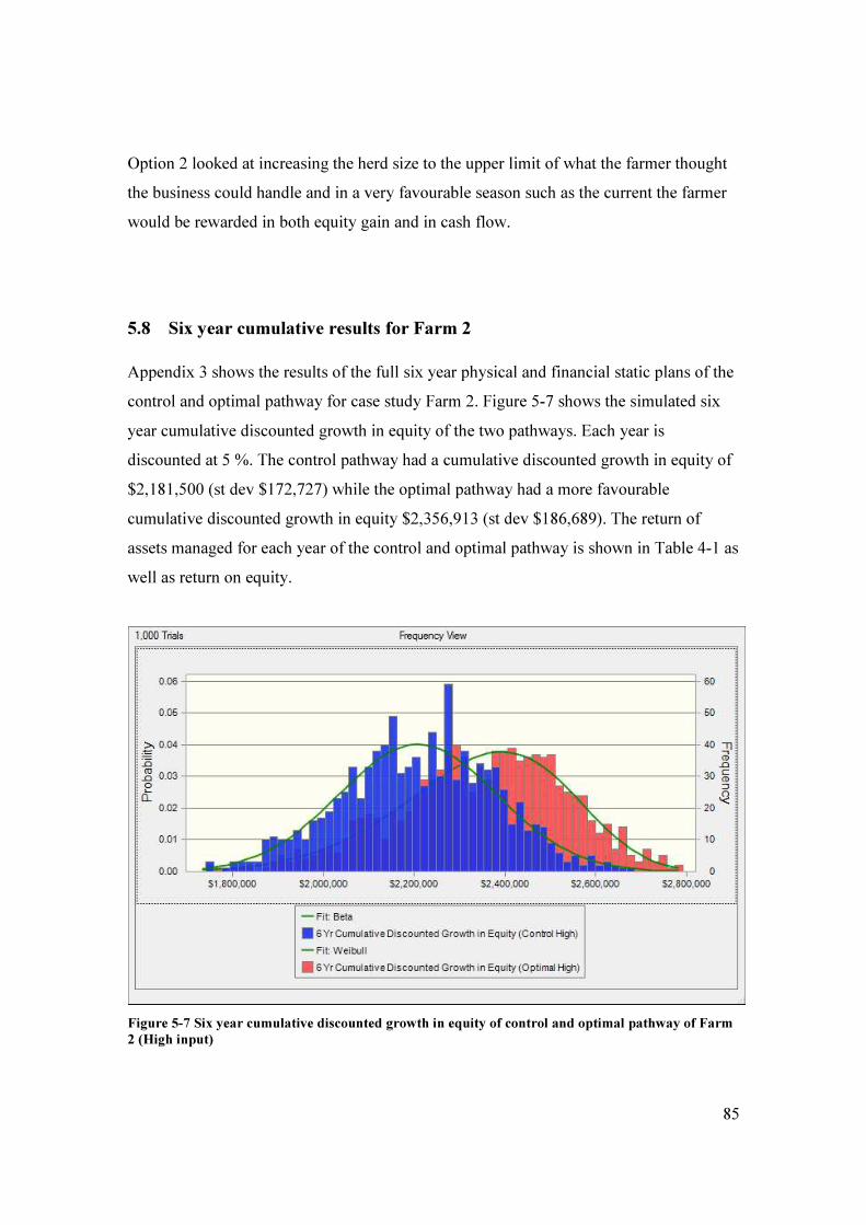
85

Option 2 looked at increasing the herd size to the upper limit of what the farmer thought

the business could handle and in a very favourable season such as the current the farmer

would be rewarded in both equity gain and in cash flow.

5.8 Six year cumulative results for Farm 2

Appendix 3 shows the results of the full six year physical and financial static plans of the

control and optimal pathway for case study Farm 2. Figure 5-7 shows the simulated six

year cumulative discounted growth in equity of the two pathways. Each year is

discounted at 5 %. The control pathway had a cumulative discounted growth in equity of

$2,181,500 (st dev $172,727) while the optimal pathway had a more favourable

cumulative discounted growth in equity $2,356,913 (st dev $186,689). The return of

assets managed for each year of the control and optimal pathway is shown in Table 4-1 as

well as return on equity.

Figure 5-7 Six year cumulative discounted growth in equity of control and optimal pathway of Farm

2 (High input)

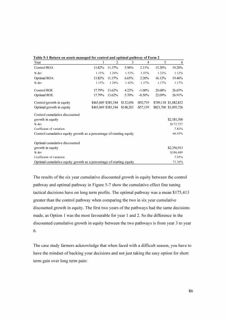
86

Table 5-1 Return on assets managed for control and optimal pathway of Farm 2

The results of the six year cumulative discounted growth in equity between the control

pathway and optimal pathway in Figure 5-7 show the cumulative effect fine tuning

tactical decisions have on long term profits. The optimal pathway was a mean $175,413

greater than the control pathway when comparing the two in six year cumulative

discounted growth in equity. The first two years of the pathways had the same decisions

made, as Option 1 was the most favourable for year 1 and 2. So the difference in the

discounted cumulative growth in equity between the two pathways is from year 3 to year

6.

The case study farmers acknowledge that when faced with a difficult season, you have to

have the mindset of backing your decisions and not just taking the easy option for short

term gain over long term pain:

Year 1 2 3 4 5 6

Control ROA 13.82% 11.37% 5.96% 2.11% 15.20% 19.20%

St dev 1.15% 1.20% 1.53% 1.47% 1.23% 1.12%

Optimal ROA 13.82% 11.37% 6.65% 2.20% 16.12% 19.46%

St dev 1.15% 1.20% 1.42% 1.37% 1.17% 1.17%

Control ROE 17.79% 13.62% 4.22% -1.00% 20.68% 26.65%

Optimal ROE 17.79% 13.62% 5.70% -0.50% 22.09% 26.91%

Control growth in equity $465,069 $381,544 $132,056 -$92,719 $749,118 $1,082,832

Optimal growth in equity $465,069 $381,544 $148,203 -$57,159 $821,700 $1,095,726

Control cumulative discounted

growth in equity $2,181,500

St dev $172,727


Control cumulative equity growth as a percentage of starting equity 66.05%

Optimal cumulative discounted

growth in equity $2,356,913

St dev $186,689


Optimal cumulative equity growth as a percentage of starting equity 71.36%

87

“When the drought started, you had your good days and bad days and we thought why not sell the farm, we decided with what we had done with the lasering, the watering and pastures, and increase in cow numbers is we made a commitment at the start we were going to be here at the end. I think without that sort of commitment you think will we do it this year or will we not do it this year, we said no were in, were going to go and we’re going to attack it, so once we’ve done that then, all this other stuff starts to fall into place. If you don’t have that mindset that your going to be around for ten years, then I don’t think we would have done anything, I think we would have just drifted along and possibly just drifted out, which is what I think a lot of people did.”

Given the views of the farming couple of Farm 2 below, the strategic analysis of selling

high security water that was analysed for case study farm 1 was not analysed for Farm 2.

They believed that it is more worthwhile to own high security water right rather than sell

it and just purchase on the temporary water market because of the risks posed by

government changes to the rules on irrigation:

“With high security water, we’ve had this debate a bit, we’re in a discussion group and we’ve had it with the discussion group, and one guy sold a lot of his high security water because he said he couldn’t justify having all that capital tied up, he’d rather buy the two farms next door with that water and he’s bought a reasonable amount of low security water to cover himself. Our view is that’s a good call, but he’s leaving himself exposed if the rules change. And the way the rules are at the moment we would want to have a significant amount of high security water because we have a major business here and that’s the insurance we pay, so it’s a very high premium, but once the capitals there, I don’t see, the price will fluctuate depending on what the government does but if your in it long haul, I don’t see the ass dropping out of permanent water, so we’ve tucked that money away, and we’re using it, and we can do it in 5 years or 10 years time if we want to do what that other guys done. We think it just provides us with a basis for the business being and we’re less at the whim of government changes. They’re not going to touch high security.”

88

6 Comparison of case study Farm 1 to Farm 2 The following diagram (Figure 6-1) shows a comparative analysis of the two case study

farms return on assets managed for their optimal pathways. Farm 1s ROA for each year is

shown by the pink line and Farm 2s ROA for each year is shown by the blue line. The

cross bars are the standard deviation of ROA’s for those particular years.

Figure 6-1 Return on Assets managed for the Optimal pathways of Farm 1 and 2

When comparing the two case study farms based on return on assets managed, Farm 2

had a greater return in all 6 years. Farm 2 also had a greater range of ROA’s over the 6

years ranging from 2.20 % in Year 4 to 19.46 % in Year 6, compared to Farm 2 with a

ROA range of 0.02 % in Year 3 to 12.26 % in Year 6.

In Year 3 when there was a drought forecast for the year, Farm 2 was able to withstand

the first year of the drought better with a ROA of 6.65 % compared to Farm 1 with a

ROA of 0.02%. The large amount of water Farm 2 was able to carry over due to its large

low security water right buffered the farm against water shortfalls. The asset of the carry

over water also increased significantly in value as the unit price increased in the drought.

In Year 4 however, the reduction in carry over water as well as a decrease in value of

temporary water decreased Farm 2s profitability and ROA, Farm 1 on the other hand had

a ROA in Year 4 that was reflective of the type of season faced – more favourable than

89

Year 3. Both farms recovered well in Year 5 and again in Year 6 with ROA’s higher than

their Year 1 ROA’s.

Farm 2 had a smaller coefficient of variation for its cumulative discounted growth in

equity of the Optimum pathway of 7.95 % compared to Farm 1 of 34 %. Farm 2 had

undertaken several steps to reduce the volatility within year and between years. This

includes undertaking a grain buying strategy to reduce their exposure to increases in

price, supplies a domestic milk manufacturing supplier, securing large carry over water

for drought proofing.

The differences between the two farms on how they reduce volatility are demonstrated in

how they purchase their grain. Case study farm 1 deals with a local grain grower and

does not lock in a price:

“We’ve been using triticale for a long time, we have an arrangement with a grower at Nagambie and he grows the grain for us, so we are able to source it competitively and we’re pretty happy with it as a feed source. Although the mix we’re using at the moment is not triticale because Reids have trouble sourcing it so its wheat.

In terms of grain contracts we’ve tried them but could never get them to work for us, we always got caught on the wrong end of the cycle, though that’s something we didn’t do during the drought.”

Case study farm 2 on the other hand prefers to deal with a grain dealer and lock in a price

“We tried to deal with cereal grain growers but they’re own worst enemies. You get half their header in the bottom of the silo going through your roller mill. And you get a bit of rain and they can’t get their truck in! ‘You’ll have to wait till next week’, but our cows can’t wait to next week. So we’ve got a relationship with another fellow who we’ve been buying grain from, he’s just an agent and a truck driver in Birchip and he’s got reasonably big now, but because he provides a good service and quality grain and those sorts of things, so we buy most of our grain through him and he’s been fairly competitive. We can take grain contracts out through him, because he’s happy to offset that with the barley board or wheat board. So if we buy grain and lock it in say at $220 for a thousand tonnes, I know that he takes a thousand tonnes the other way with the barley board so he’s not exposed”

Farm 2 goes even further to take the volatility out of other costs as well:

“We’ve had contracts for power, you can sign a contract with a power company for 12 months and you know your costs. I think we had 2 year contracts a couple of years back. Herd costs I control all that, because in the drought and in the early stages because I select the

90

bulls, I select of mix of proven and progeny tests. We mix our own grain because it’s cheaper than buying Ian Reid.”

Seven years ago Farm 2 switched milk supply companies from an export manufacturing

company to a domestic company. Their flat line production was well suited for domestic

production and there was a greater premium paid, as well as fixed price contracts that

enabled them to avoid the worst of price step-down in 2009:

“So in the second year of the drought we left Murray Goulburn and went to Dairy Farmers, and just by sending a different tanker down the driveway we made another $120,000, and that was significant. And with the step down we kept our price up, so it’s probably worth I reckon over 6 or 7 years half a million dollars, as compared to being with Murray Goulburn or Fonterra. And we’ve got people who milk similar numbers of cows to us but they’re with an export company and their still having issues with cash flow even this year in the spring.”

Both farms also vary in their thought process on how they would treat labour in a very

poor economic year. Farm 1 describes that reducing labour was one of the options

available during the last drought:

“[There were] certainly times when the workload increased significantly because we went through periods where we had either no labour or a reduced amount of labour. We’ve returned to probably better than normality at the moment because again probably because of my age. We’ve got more labour than we’ve ever had at the moment.”

Farm 2 indicated that labour was not an option for reducing costs in a drought because it

may end up costing them more in the future from bad decisions from fatigue:

“Labours a small part of a whole cost. I don’t think that when things are tight that that should be the one to go, in fact I’ve never really thought of doing that because when things are tight, (wife) and I need to be thinking straight. So if I pull someone out of the dairy or make someone work 12 hrs a week less, at the moment its not as if someone is standing around where we can pull someone out 12 hrs a week and we wont notice a difference. It’s all pretty tight because I’m there every day. So if I pulled him out, I’d have to step in, I might be better at it, I might do it in 8 hrs but I’d be tired and stressed and I wouldn’t make a good decision, and I wouldn’t buy that right hay, so you can penny pinch.”

91

7 Conclusion This thesis has studied two contrasting northern Victorian irrigated pasture based dairy

farm systems, one a ‘medium input’ and the other a ‘high input’. The research aimed to

evaluate the nature and implications of options facing the managers of two pasture based

dairy farm businesses operated at medium and high levels of input use and trying to

minimize losses in unfavourable seasons and maximize profits in favourable seasons.

The investigation found that both farming systems had different optimum choices

available year to year to increase profitability. Further, the nature of the choices differed

between the medium and high input farms.

The study found there is merit in assessing tactical decision options on an annual basis

since decisions taken and market and climatic circumstances in each unique year always

result in different financial outcomes. For both farms, in years with greater upside, there

was a greater range of outcomes between decisions compared to years with poor financial

outcomes.

For both farms, in years with greater upside, there was a greater range of outcomes

between decisions compared to years with poor financial outcomes. This suggests farm

managers cannot get too relaxed and complacent in the good years and need to ensure

they are gaining the benefits of the good year as well as minimizing losses in the poor

years.

Both farms in the study had similar pasture setups, with two thirds permanent pasture and

one third lucerne. Both had similar strategies in previous droughts of not irrigating the

permanent pasture from late December to February. During the simulated drought half

way through the six year analysis, both farms were more profitable reducing their pasture

growth in the middle of the summer to save water and reducing their herd size to a level

that still allows them to ‘bounce back’ when the more favourable season returns.

‘Medium’ input farms decision options were different from ‘High’ input farms options.

92

For ‘Medium’ input farm, there were decisions on the quantity and quality of

concentrates fed, production levels per cow, stocking rate and level of pasture production

in dry seasons. ‘High’ input farm was more profitable keeping production per cow over

8000 L in both the favourable and unfavourable seasons, however adjusting the herd size

was very important for tackling the unfavourable seasons and making the most of the

favourable seasons. ‘High’ input farm was set up very well to buffer itself against

droughts in the analysis by carrying over two years worth of water supply. Two

advantages were gained from the carryover; firstly there was no shortfall of irrigation

water during the drought, and also the value of the water increases during dry periods

which have positive effects on the balance sheet and profit and loss statement. Cash flow

is also more favourable with the carry over as the water does not have to be purchased

during unfavourable water markets.

The two farms started the 6 year period in different situations of financial strength and

vulnerability. ‘Medium’ input farm had total assets of $3,497,996, medium and long term

debt of $1,169,000 and equity of $2,328,996 at 67 % of assets. ‘High’ input farm had

total assets of $4,962,426, medium and long term debt of $2,016,558 and equity of

$2,945,868 at 59 % of assets.

By following paths of ‘best options’ over the 6 consecutive years, ‘Medium’ input farm

added $190,301 (st dev $64,663) in real terms to their net worth discounted at a 5 % real

rate and ‘High’ input farm added $2,356,913 (st dev $186,689) in real terms to their net

worth discounted at a 5 % real rate. The addition to their net worth represented an

increase to their starting equity of 7.64 % for Farm 1 and 71.36 % for Farm 2.

‘Medium’ input farms balance sheet at the end of year 6 in real terms (in 2012 dollars)

had assets of $3,628,498, liabilities of $959,000 and equity of $2,669,498 at 74% of

assets. ‘High’ input farm in real terms had assets of $7,954,782 liabilities of $2,016,558

and equity of $5,938,224 at 75 % of assets.

93

For ‘Medium’ input farm the ‘optimal’ pathway had a growth in equity mean of $100,241

greater than that of the ‘control’ pathway. However, this value difference is not the

difference between its worst possible outcomes and its best possible outcomes. The

‘control’ pathway is limited to the assumptions derived from the farmer’s answers at

interview on what they would do under various circumstances. The ‘optimum’ pathway is

a result of testing particular tactical strategies to determine the most favourable pathway

financially. For ‘High’ input farm, the ‘optimal’ pathway had a growth in equity mean of

$175,413 greater than that of the ‘control’ pathway.

The medium input farm did not build the wealth from farming over the six years

compared to the high input farm. This was due to in part of the smaller size and scale, it

had relatively high overheads per kg MS output that it had to cover. This farming system

suited the farmer given his age with no family succession, however for a young farmer in

this system, they will have to keep growing and developing the business in order to gain

wealth. There may be extra growth from increase in land and water values above inflation

in the current system and changes in discretionary spending was not looked at in the

analysis, however still would not have a large effect.

In many of the scenarios tested, the decision option with the highest growth in equity

compared to other options tested did not always result in the highest net cash flow. The

decision maker would need to evaluate the net cash flow implications of their decisions to

determine if they are worthwhile choices.

For ‘Medium’ input farm, the strategic strategy of selling 500 ML of high security water

right with and with out purchasing 500 ML of low security water right was looked at. The

sale of 500 ML of water in year 1 of the ‘optimal’ pathway resulted in a mean six year

cumulative discounted growth in equity of $253,146 (st dev $60,875), an improvement of

around $56,000 compared to not selling the water. The purchase of 500 ML of low

security water right with the sale of 500 ML of high security water right in Year 1

resulted in the most favourable outcome with the mean six year cumulative discounted

growth in equity increasing to $280,847 (st dev $58,543), an increase of around $84,000

94

compared to not selling the water. It allowed the business to safely carry more temporary

water over into the drought years, to ease the water burden in the drought and to reduce

the impact of year to year climatic volatility.

With a large business, ‘High’ input farm actively reduced volatility both within year and

between years. The farming couple has a strategy for locking in costs for grain and fodder

within the year and have a strategy of keeping two years supply of carry over water to

protect from between year climatic volatility. They also supplied a domestic milk

manufacturing company that suited their flat milk supply.

The ‘High’ input farm had a greater range of Return on assets managed over the run of 6

years ranging from 2.20 % in Year 4 to 19.46 % in Year 6, compared to Farm 2 with a

return on assets managed range of 0.02 % in Year 3 to 12.26 % in Year 6.

The biophysical and economic performance analysis performed over a six year period of

varying climatic and economic conditions was used to analyse each case study farms

tactical farm management decision options. The methodology used in the study was

found to be quite practical, flexibly accommodating the different farming systems

involved in the study and processing the data in a respectable time.

95

8 Appendix 1 - Case Study Interview Questionnaire

A. TECHNICAL, PRODUCTION AND HUSBANDRY ISSUES

1. Describe your approach to Pasture Species & Grazing management

a) What was your irrigated pasture base during this era?

b) What did you think was your optimum stocking rate?

c) What was your approach to grazing management based upon? (e.g. rotation length, pasture cover, leaf stage)

2. Tell me about your Soil, Water & Irrigation management

a) What was your view on the future of irrigation in the region during this era?

b) What were the main threats to your business associated with irrigation: - water tables and salinity?

- unpredictability? - politics?

c) What was your approach to soil health, fertility and fertilizer policy?

3. Describe what you focused on with your Cow Husbandry & Herd Size management

a) What was your approach to calving pattern b) What was your approach to cow fertility c) What was your approach to herd size- keep growing every season – sell export heifers?

d) What was your approach to heifer rearing? e) What about body condition – did you routinely monitor it?

f) What about cow productivity and milk yields? 4. What Feeding Strategies & Supplementary Feeds did you use during this era?

a) How would you describe your feeding system during this era? b) What was your view on grain feeding in this era:

- used to fill shortfalls in feed gaps? - used to increase production and returns?

- what type of concentrates did you use?

- did you use lead feeding in your herd? c) Where did your supply of supplementary feeds come from?

- Did you grow any fodder crops and, if so, what types? -Did you conserve them yourself?

d) How did you respond to above and below average climate years with your feeding strategy?

B. FINANCIAL AND DEBT-SERVICING ISSUES

1. Tell me about your experiences and preferences regarding Banks & Borrowing during this era? a) How would you describe your level of indebtedness during this era? b) Where you an aggressive or conservative borrower during this era? c) Is the bank you were with during this era still your main bank?

d) How did interest rates affect your borrowing decisions?

e) On what assets where you prepared to borrow against? - land, improvements & water?

96

- plant, machinery & vehicles? - livestock?

2. Describe how you carried out Cash Flow management during this era

a) Did you have any particular method of cost control, relative to herd, shed, feed, labour and overhead costs

b) Did cash flow issues ever have an impact on your chosen calving pattern?

c) Did cash flow issues ever have an impact on your approach to employing people? d) Did cash flow issues ever have an impact on your chosen feeding strategy?

e) How much did cash flow impact on your day to day decisions? Greatly? Moderately? Not at all? 3. What can you tell me about your Capital Works & Farm Development spending during this time?

a) What were the major capital works and farm developments that you conducted during this

era?

- How did you analyse your investment decisions e.g. own budgeting? professional advice? Both?

- Why did you choose to make those investments?

- to fully utilize other resources.

- for a greater return on capital.

- other reasons. What? - How new was the technology that you invested in? Were you an early adopter or did you wait for greater information and or a decrease in price

- How well did the capital works or farm development fit your existing system?

- Did it take long to iron the bugs out or adapt it?

-Did it hamper your business growth for a short period afterwards? b) What capital works or farm development did you consider investing in but ultimately chose

not to? - Why did you reject the capital works idea?

C. PEOPLE AND DECISION-MAKING ISSUES

1. Tell me about your personal Workload, Type of work, and Paid labour during this era.

a) What was predominantly your day to day work? b) How big was your workload in hours per week

c) What was the extent to which you relied upon paid labour? d) How would you describe your approach to managing labour within your system?

2. Describe how you carried out Tactical or Annual Planning & Budgeting during this era.

a) What was your annual planning approach?

b) How did you go about making tactical annual decisions? c) How did you react to sudden major changes that your business was facing i.e. milk price

collapse

3. Tell me about your Strategic Long-term Planning & Budgeting – how was it done during this era?

a) What was your long term planning approach? Formal assessment? Informal assessment?

b) What was your normal planning horizon? 5 years? Ten years? 15 years?

97

c) Who was your main reference point in making your long term plans? Family member? Banker? Professional adviser?

4. Describe how you accounted for Risk in your farm management during this era.

a) What was your approach to risk management in this era? b) How did you respond to a dry season? c) How did you respond to a wet season?

d) Did you try anything to mitigate increasing input and output price volatility? e) For this era, would you consider yourself a risk-taking gambler who plays the odds or a

conservative gambler aiming to minimize potential downside losses?

98

9 Appendix 2 – Case study Farm 1

9.1 Probabilistic ranges set for Farm 1

Probabilistic range assumptions Year 1 Year 2 Year 3 Year 4 Year 5 Year 6

Water allocation %

Min 90% 75% 25% 30% 50% 90%

Likely 100% 90% 30% 40% 80% 99%

Max 100% 100% 45% 50% 100% 100%

Temp water price ($/ML)

Min $15 $50 $250 $200 $25 $15

Likely $25 $90 $300 $250 $50 $25

Max $50 $120 $350 $300 $75 $50

Operating cost per cow* (excludes supplements, fodder conservation and temporary water purchases)

Min $1,161 $1,197 $1,267 $1,263 $1,275 $1,288

Likely $1,231 $1,267 $1,337 $1,333 $1,345 $1,358

Max $1,301 $1,337 $1,407 $1,403 $1,415 $1,428

Pasture utilised (tDM/ha)

Min 11.5 11.5 8.0 8.0 11.5 11.5

Likely 12.8 12.8 9.0 9.0 12.8 12.8

Max 13.5 13.5 10.0 10.0 13.5 13.5

Pasture utilised per cow (tDM)

Min 2.8 2.8 2.8 2.8 2.8 2.8

Likely 3.3 3.3 3.3 3.3 3.3 3.3

Max 3.5 3.5 3.5 3.5 3.5 3.5

Pasture quality (ME)

Min 10.3 10.3 10.3 10.3 10.3 10.3

Likely 10.5 10.5 10.5 10.5 10.5 10.5

Max 10.7 10.7 10.7 10.7 10.7 10.7

Pasture quality (NDF)

Min 40% 40% 40% 40% 40% 40%

Likely 41% 41% 41% 41% 41% 41%

Max 42% 42% 42% 42% 42% 42%

Milk price ($/kgMS)

Min $4.60 $4.55 $4.78 $5.28 $5.63 $5.75

Likely $4.85 $4.80 $5.03 $5.53 $5.88 $6.00

Max $5.10 $5.05 $5.28 $5.78 $6.13 $6.25

Purchased fodder ($/tDM)

Min $100 $160 $290 $240 $140 $140

Likely $140 $200 $330 $280 $180 $180

Max $180 $240 $370 $320 $220 $220

Concentrates ($/tDM)

Min $210 $310 $380 $330 $260 $170

Likely $250 $350 $420 $370 $300 $210

Max $290 $390 $460 $410 $340 $250

9.2 Farm 1 six year plan Control

Table 9-1 Physical assumptions for Control Farm 1 Physical Assumptions Previous Year Year 1 Year 2 Year 3 Year 4 Year 5 Year 6

Land

Milking Area 90 90 90 90 90 90 90

Total Area 263 263 263 263 263 263 263

Livestock

Herd Size 300 300 310 280 300 310 320

Stocking rate (cows/ha) 3.33 3.33 3.44 3.11 3.33 3.44 3.56

Bull No's. 3 3 3 3 3 3 3

R1 No's. 97 97 100 100 100 100 100

R2 No's. 73 73 95 95 95 95 95

Water

Water Allocation 0% 100% 90% 30% 40% 80% 100%

Water Use Efficiency (t/ML) 0.00 2.00 2.00 1.90 1.90 2.00 2.00

High security water share 0 739 739 739 739 739 739

Carry over water from previous season 0 525 600 600 350 160 200

Carry over water into next season 0 600 600 350 160 200 300

Water Irrigated (ML) 0 662 662 490 490 662 662

Temporary water purchased (ML) 0 -1 -3 19 5 111 23

Pasture Utilisation (tDM/ha) 12.65 12.80 12.80 9.00 9.00 12.80 12.80

Total Supplements

Concentrates (tDM) 497 531 560 475 520 499 552

Purchased fodder (tDM) 153 231 269 480 564 283 313

Home grown fodder (tDM) 317 260 240 100 100 200 200

Other feeds (tDM) 35 0 0 0 0 0 0

Diet per Cow

Concentrates (tDM/cow) 1.66 1.77 1.81 1.69 1.73 1.61 1.73

Purchased fodder (tDM/cow) 0.51 0.77 0.87 1.71 1.88 0.91 0.98

Home grown fodder (tDM/cow) 1.06 0.87 0.77 0.36 0.33 0.65 0.63

Other feeds (tDM/cow) 0.12 0.00 0.00 0.00 0.00 0.00 0.00

Pasture (tDM/cow) 2.74 2.97 2.94 2.54 2.37 3.07 2.98

Total 6.08 6.38 6.39 6.30 6.31 6.24 6.31

NDF Content of Diet

Concentrates (NDF %) 18% 18% 18% 18% 18% 18% 18%

Purchased fodder (NDF %) 57% 55% 55% 50% 50% 50% 50%

Home grown fodder (NDF %) 55% 50% 50% 60% 60% 60% 60%

Other feeds (NDF %) 55% 55% 6% 6% 6% 6% 6%

Pasture (NDF%) 41% 41% 41% 41% 41% 41% 41%

Total Diet NDF % 38% 36% 36% 37% 37% 37% 37%

Metabolisable energy content of Diet

Concentrates (MJ ME/kgDM) 12 12 12.0 12.0 12.0 12.0 12.0

Purchased fodder (MJ ME/kgDM) 8.0 8.0 8.0 9.0 9.5 9.0 9.0

Home grown fodder (MJ ME/kgDM) 9.0 9.0 9.0 9.0 9.0 9.0 9.0

Other feeds (MJ ME/kgDM) 10.0 10.0 6.0 6.0 6.0 6.0 6.0

Pasture (MJ ME/kgDM) 10.5 10.5 10.5 10.5 10.5 10.5 10.5

Total Diet MJ ME/kgDM 10.5 10.2 10.1 10.2 10.3 10.3 10.3

Cow intake and energy settings

Rumen Fill 98% 100% 100% 100% 100% 100% 100%

Body Condition Change 0.25 0.25 0.25 0.25 0.25 0.25 0.25

Maintenance increment 8% 8% 8% 8% 8% 8% 8%

Fodder Wastage 10% 10% 10% 10% 10% 10% 10%

Milk Production

Fat % 4.3% 4.3% 4.3% 4.3% 4.3% 4.3% 4.3%

Protein % 3.6% 3.6% 3.5% 3.5% 3.5% 3.5% 3.5%

Milk production (L/cow) 5,428 5,949 6,003 5,786 5,903 5,886 5,997

Milk production (kgMS/cow) 429 470 468 451 460 459 468

Total milk production (L) 1,628,430 1,784,821 1,860,903 1,620,120 1,770,947 1,824,760 1,918,897

Total milk production (kgMS) 128,603 141,001 145,150 126,369 138,134 142,331 149,674

0.89 0.93 0.94 0.92 0.93 0.94 0.95

Feed conversion efficiency

(L/kgDM food offered)

Table 9-2 Price assumptions for Control Farm 1

Table 9-3 Balance sheet options Control Farm 1

Balance Sheet 2010 Open 2011 Close 2012 Opening Year 1 Year 2 Year 3 Year 4 Year 5 Year 6

Assets:

Current Assets:

Total livestock value $475,770 $491,051 $491,051 $525,501 $525,501 $499,501 $525,501 $538,501 $551,501

Fodder Inventory $8,680 $94,924 $94,924 $94,924 $94,924 $94,924 $94,924 $94,924 $94,924

Carry over water $1,490 $4,500 $4,500 $15,000 $54,000 $105,000 $40,000 $10,000 $7,500

Other Assets $0 $0 $0 $0 $0 $0 $0 $0 $0

Cash $0 $113,970 $0 -$18,027 -$77,398 -$256,502 -$350,426 -$237,743 -$29,722

Total Current Assets $485,940 $704,445 $590,475 $617,398 $597,027 $442,923 $309,999 $405,682 $624,203

Non Current Assets

Total land value (ex dairy) $1,682,937 $1,682,937 $1,682,937 $1,682,937 $1,682,937 $1,682,937 $1,682,937 $1,682,937 $1,682,937

High security water $1,108,500 $1,108,500 $1,108,500 $1,108,500 $1,108,500 $1,108,500 $1,108,500 $1,108,500 $1,108,500

Dairy $0 $0 $0 $0 $0 $0 $0 $0 $0

Plant and equipment $105,000 $116,084 $116,084 $104,476 $94,028 $84,625 $76,163 $68,546 $61,692

Factory Shares $145,242 $0 $0 $0 $0 $0 $0 $0 $0

Total Non Current Assets $3,041,679 $2,907,521 $2,907,521 $2,895,913 $2,885,465 $2,876,062 $2,867,600 $2,859,983 $2,853,129

Total Assets $3,527,619 $3,611,966 $3,497,996 $3,513,311 $3,482,492 $3,318,985 $3,177,599 $3,265,665 $3,477,331

Liabilities:

Fixed interest loans $1,249,000 $1,169,000 $1,169,000 $1,134,000 $1,099,000 $1,064,000 $1,029,000 $994,000 $959,000

Variable interest loans $0 $0 $0 $0 $0 $0 $0 $0 $0

HP Loans $0 $0 $0 $0 $0 $0 $0 $0 $0

New loans $0 $0 $0 $0 $0 $0 $0 $0 $0

Cow lease $0 $0 $0 $0 $0 $0 $0 $0 $0

Trade creditors $0 $0 $0 $0 $0 $0 $0 $0 $0

Total Liabilities $1,249,000 $1,169,000 $1,169,000 $1,134,000 $1,099,000 $1,064,000 $1,029,000 $994,000 $959,000

Equity: $2,278,619 $2,442,966 $2,328,996 $2,379,311 $2,383,492 $2,254,985 $2,148,599 $2,271,665 $2,518,331

Growth in Equity $0 $164,347 $0 $50,315 $4,181 -$128,507 -$106,386 $123,066 $246,666

Equity % 65% 68% 67% 68% 68% 68% 68% 70% 72%

Price Assumptions Previous Year Year 1 Year 2 Year 3 Year 4 Year 5 Year 6

Operating Price Assumptions

Fixed operating costs per cow* $404 $404 $399 $451 $429 $423 $418

Variable operating costs per cow* $852 $852 $868 $886 $904 $922 $940

Total operating costs per cow* $1,256 $1,256 $1,267 $1,337 $1,333 $1,345 $1,358

Temporary water price ($/ML) $25 $90 $300 $250 $50 $25

Milk price (Factory standard $/kgMS) $4.85 $4.80 $5.03 $5.53 $5.88 $6.00

Milk price received ($/kgMS) $5.43 $4.88 $4.82 $5.05 $5.55 $5.90 $6.02

Milk price (c/L) 42.9 38.5 37.6 39.4 43.3 46.0 47.0

Concentrates ($/tDM) $219 $250 $350 $420 $370 $300 $210

Purchased fodder price ($/tDM) $140 $140 $200 $330 $280 $180 $180

Home Grown Fodder price ($/tDM) $140 $140 $140 $130 $130 $130 $130

Other Feeds price ($/tDM) $248

Concentrates fixed price ($/tDM) $330 $350 $420 $370 $300 $210

Options Price ($/tDM) $350 $350 $350 $350 $350 $350

Options Premium ($/tDM) $10 $10 $10 $10 $10 $10

Percentage of concentrates spot price 100% 100% 100% 100% 100% 100%

Percentage of concentrates fixed price

Percentage of concentrates options price

Balance Sheet Price Assumptions

Land Value per hectare $6,399 $6,399 $6,399 $6,399 $6,399 $6,399 $6,399

Cow value $1,300 $1,300 $1,300 $1,300 $1,300 $1,300 $1,300

High security water value $1,500 $1,500 $1,500 $1,500 $1,500 $1,500 $1,500

*Operating costs exclude supplements, fodder conservation and temporary water purchases

101

Table 9-4 Profit and loss statement Control Farm 1

Table 9-5 Cash flow statement Control Farm 1

Profit and Loss Previous Year Year 1 Year 2 Year 3 Year 4 Year 5 Year 6

Milk income $698,591 $687,663 $699,402 $638,082 $766,818 $840,127 $901,498

Livestock trading profit (loss) $50,678 $60,450 $56,000 $44,000 $68,000 $62,000 $62,000

Fodder inventory change $86,244 $0 $0 $0 $0 $0 $0

Land and HS Water trading $0 $0 $0 $0 $0 $0 $0

Carry over water $3,010 $10,500 $39,000 $51,000 -$65,000 -$30,000 -$2,500

Other income $9,149 $10,000 $10,000 $13,000 $13,000 $13,000 $13,000

Gross farm income $847,672 $768,613 $804,402 $746,082 $782,818 $885,127 $973,998

Supplement costs $183,206 $201,527 $283,216 $370,629 $363,369 $226,774 $198,380

Non Supplement operating costs $327,812 $376,800 $392,770 $374,360 $399,900 $416,950 $434,560

Temporary water purchases (sales) $12,000 -$22 -$243 $5,569 $1,166 $5,560 $585

Depreciation $10,500 $11,608 $10,448 $9,403 $8,463 $7,616 $6,855

Imputed labour $49,000 $49,000 $49,000 $49,000 $49,000 $49,000 $49,000

Gross farm costs $533,518 $589,914 $686,190 $759,960 $772,897 $656,900 $640,380

Earnings before Interest & Tax (EBIT) $314,154 $178,699 $118,212 -$13,878 $9,921 $228,226 $333,618

Total assets managed $3,569,792 $3,505,653 $3,497,901 $3,400,739 $3,248,292 $3,221,632 $3,371,498

Return on asset 8.80% 5.10% 3.38% -0.41% 0.31% 7.08% 9.90%

Interest $97,880 $93,455 $98,683 $109,150 $113,307 $102,160 $83,951

Lease $0 $0 $0 $0 $0 $0 $0

Bank Charges $2,927 $2,927 $3,000 $3,000 $3,000 $3,000 $3,000

Total finance costs $100,807 $96,382 $101,683 $112,150 $116,307 $105,160 $86,951

Net farm income $213,347 $82,317 $16,529 -$126,028 -$106,386 $123,066 $246,666

Return on equity 18.32% 3.50% 0.69% -5.43% -4.83% 5.57% 10.30%

Consumption $0 $0 $0 $0 $0 $0 $0

Taxable income $213,347 $82,317 $16,529 -$126,028 -$106,386 $123,066 $246,666

Losses carried forward $0 $0 $0 $0 -$126,028 -$232,414 -$109,348

Tax payable from previous year @ 15% $0 $32,002 $12,348 $2,479 $0 $0 $0

Growth in Equity $213,347 $50,315 $4,181 -$128,507 -$106,386 $123,066 $246,666

Discounted Growth in Equity @ 5% $213,347 $47,919 $3,793 -$111,009 -$87,524 $96,425 $184,066

Std. Deviation Discounted Growth in Equity $0 $21,989 $22,169 $21,909 $21,180 $20,934 $20,146

Cumulative Discounted Growth in Equity $47,919 $51,711 -$59,298 -$146,822 -$50,396 $133,670

Std. Deviation Cumulative Discounted Growth in Equity $61,651

Cash Flow Previous Year Year 1 Year 2 Year 3 Year 4 Year 5 Year 6

Milk income $698,591 $687,663 $699,402 $638,082 $766,818 $840,127 $901,498

Livestock income $35,397 $26,000 $56,000 $70,000 $42,000 $49,000 $49,000

Other income $9,149 $10,000 $10,000 $13,000 $13,000 $13,000 $13,000

New Loans and Borrowings $0 $0 $0 $0 $0 $0 $0

Non Bank capital injections $0 $0 $0 $0 $0 $0 $0

Land and High Security Water sales $0 $0 $0 $0 $0 $0 $0

Total cash income $743,137 $723,663 $765,402 $721,082 $821,818 $902,127 $963,498




Total operating costs $474,018 $529,306 $626,743 $701,558 $715,435 $600,284 $584,525

Lease $0 $0 $0 $0 $0 $0 $0

Interest $100,807 $96,382 $101,683 $112,150 $116,307 $105,160 $86,951

Principal $80,000 $35,000 $35,000 $35,000 $35,000 $35,000 $35,000

Drawings $49,000 $49,000 $49,000 $49,000 $49,000 $49,000 $49,000

Land and High Security Water purchases $0 $0 $0 $0 $0 $0 $0

Plant and Machinery Purchases $21,584 $0 $0 $0 $0 $0 $0

Factory share Purchases -$145,242 $0 $0 $0 $0 $0 $0

Farm capital works $0 $0 $0 $0 $0 $0 $0

Total capital and finance $106,149 $180,382 $185,683 $196,150 $200,307 $189,160 $170,951

Net cash flow before Tax $162,970 $13,975 -$47,024 -$176,625 -$93,923 $112,682 $208,021

Tax $0 $32,002 $12,348 $2,479 $0 $0 $0

Net cash flow after tax $162,970 -$18,027 -$59,371 -$179,104 -$93,923 $112,682 $208,021

102

9.3 Farm 1 Optimal 6 year alternative

Table 9-6 Physical assumptions Optimal Farm 1

Physical Assumptions Previous Year Year 1 Year 2 Year 3 Year 4 Year 5 Year 6

Land

Milking Area 90 90 90 90 90 90 90

Total Area 263 263 263 263 263 263 263

Livestock

Herd Size 300 330 310 280 300 330 345


Bull No's. 3 3 3 3 3 3 3

R1 No's. 97 97 100 100 100 100 100

R2 No's. 73 73 95 95 95 95 95

Water






Water Irrigated (ML) 0 662 662 490 786 662 662

Temporary water purchased (ML) 0 -1 -3 19 300 111 23


Total Supplements

Concentrates (tDM) 497 615 560 603 602 667 711

Purchased fodder (tDM) 153 342 269 429 271 319 390


Other feeds (tDM) 35 0 0 0 0 0 0

Diet per Cow





Pasture (tDM/cow) 2.74 2.76 2.94 2.54 3.10 2.88 2.88

Total 6.08 6.39 6.39 6.58 6.51 6.48 6.53

NDF Content of Diet




Other feeds (NDF %) 55% 55% 6% 6% 6% 6% 6%

Pasture (NDF%) 41% 41% 41% 41% 41% 41% 41%

Total Diet NDF % 38% 36% 36% 35% 35% 36% 35%


Concentrates (MJ ME/kgDM) 12 12 12.0 12.8 12.8 12.8 12.8







Rumen Fill 98% 100% 100% 100% 100% 100% 100%



Fodder Wastage 10% 10% 10% 10% 10% 10% 10%

Milk Production

Fat % 4.3% 4.3% 4.3% 4.1% 4.2% 4.1% 4.1%

Protein % 3.6% 3.6% 3.5% 3.5% 3.5% 3.5% 3.5%





0.89 0.92 0.94 1.05 1.06 1.05 1.06



103

Table 9-7 Price assumptions Optimal Farm 1

Table 9-8 Balance sheet Optimal Farm 1


Assets:

Current Assets:

Total livestock value $475,770 $491,051 $491,051 $551,501 $525,501 $499,501 $525,501 $564,501 $584,001


Carry over water $1,490 $4,500 $4,500 $15,000 $54,000 $105,000 $40,000 $10,000 $7,500

Other Assets $0 $0 $0 $0 $0 $0 $0 $0 $0

Cash $0 $162,970 $0 -$35,247 -$78,281 -$250,419 -$310,450 -$178,813 $88,944

Total Current Assets $485,940 $753,445 $590,475 $626,178 $596,144 $449,006 $349,975 $490,612 $775,369

Non Current Assets


High security water $1,108,500 $1,108,500 $1,108,500 $1,108,500 $1,108,500 $1,108,500 $1,108,500 $1,108,500 $1,108,500

Dairy $0 $0 $0 $0 $0 $0 $0 $0 $0


Factory Shares $145,242 $0 $0 $0 $0 $0 $0 $0 $0


Total Assets $3,527,619 $3,660,966 $3,497,996 $3,522,090 $3,481,609 $3,325,068 $3,217,575 $3,350,595 $3,628,498

Liabilities:

Fixed interest loans $1,249,000 $1,169,000 $1,169,000 $1,134,000 $1,099,000 $1,064,000 $1,029,000 $994,000 $959,000


HP Loans $0 $0 $0 $0 $0 $0 $0 $0 $0

New loans $0 $0 $0 $0 $0 $0 $0 $0 $0

Cow lease $0 $0 $0 $0 $0 $0 $0 $0 $0

Trade creditors $0 $0 $0 $0 $0 $0 $0 $0 $0

Total Liabilities $1,249,000 $1,169,000 $1,169,000 $1,134,000 $1,099,000 $1,064,000 $1,029,000 $994,000 $959,000

Equity: $2,278,619 $2,491,966 $2,328,996 $2,388,090 $2,382,609 $2,261,068 $2,188,575 $2,356,595 $2,669,498

Growth in Equity $0 $213,347 $0 $59,094 -$5,481 -$121,541 -$72,494 $168,020 $312,903

Equity % 65% 68% 67% 68% 68% 68% 68% 70% 74%




Variable operating costs per cow* $852 $852 $869 $886 $904 $922 $940


Temporary water price ($/ML) $0 $25 $90 $300 $250 $50 $25

Milk price (Factory standard $/kgMS) $0.00 $4.85 $4.80 $5.03 $5.53 $5.88 $6.00


Milk price (c/L) 42.9 38.5 37.6 38.8 43.0 45.3 46.3




Other Feeds price ($/tDM) $248 $0 $0 $0 $0 $0 $0

Concentrates fixed price ($/tDM) $0 $330 $350 $420 $370 $300 $210

Options Price ($/tDM) $0 $350 $350 $350 $350 $350 $350

Options Premium ($/tDM) $0 $10 $10 $10 $10 $10 $10

Percentage of concentrates spot price 0% 100% 100% 100% 100% 100% 100%

Percentage of concentrates fixed price 0% 0% 0% 0% 0% 0% 0%

Percentage of concentrates options price 0% 0% 0% 0% 0% 0% 0%



Cow value $1,300 $1,300 $1,300 $1,300 $1,300 $1,300 $1,300

High security water value $1,500 $1,500 $1,500 $1,500 $1,500 $1,500 $1,500


104

Table 9-9 Profit and loss statement Optimal Farm 1

Table 9-10 Cash flow statement Optimal Farm 1


Milk income $698,591 $747,571 $699,402 $746,563 $892,801 $1,017,587 $1,100,627


Other income $9,149 $10,000 $10,000 $13,000 $13,000 $13,000 $13,000

New Loans and Borrowings $0 $0 $0 $0 $0 $0 $0



Total cash income $743,137 $770,571 $779,402 $829,563 $947,801 $1,065,587 $1,159,127




Total operating costs $474,018 $588,528 $623,023 $804,774 $810,487 $749,155 $728,511

Lease $0 $0 $0 $0 $0 $0 $0

Interest $100,807 $101,288 $101,748 $111,699 $113,346 $100,795 $78,859

Principal $80,000 $35,000 $35,000 $35,000 $35,000 $35,000 $35,000

Drawings $49,000 $49,000 $49,000 $49,000 $49,000 $49,000 $49,000



Factory share Purchases -$145,242 $0 $0 $0 $0 $0 $0

Farm capital works $0 $0 $0 $0 $0 $0 $0


Net cash flow before Tax $162,970 -$3,245 -$29,369 -$170,911 -$60,031 $131,637 $267,758

Tax $0 $32,002 $13,664 $1,228 $0 $0 $0

Net cash flow after tax $162,970 -$35,247 -$43,033 -$172,138 -$60,031 $131,637 $267,758


Milk income $698,591 $747,571 $699,402 $746,563 $892,801 $1,017,587 $1,100,627


Fodder inventory change $86,244 $0 $0 $0 $0 $0 $0

Land and HS Water trading $0 $0 $0 $0 $0 $0 $0

Carry over water $3,010 $10,500 $39,000 $51,000 -$65,000 -$30,000 -$2,500

Other income $9,149 $10,000 $10,000 $13,000 $13,000 $13,000 $13,000

Gross farm income $847,672 $841,521 $792,402 $854,563 $908,801 $1,074,587 $1,176,127




Depreciation $10,500 $11,608 $10,448 $9,403 $8,463 $7,616 $6,855

Imputed labour $49,000 $49,000 $49,000 $49,000 $49,000 $49,000 $49,000

Gross farm costs $533,518 $649,137 $682,470 $863,177 $867,949 $805,771 $784,366

Earnings before Interest & Tax (EBIT) $314,154 $192,384 $109,932 -$8,614 $40,852 $268,815 $391,762


Return on asset 8.74% 5.48% 3.14% -0.25% 1.25% 8.19% 11.23%

Interest $97,880 $98,361 $98,748 $108,699 $110,346 $97,795 $75,859

Lease $0 $0 $0 $0 $0 $0 $0

Bank Charges $2,927 $2,927 $3,000 $3,000 $3,000 $3,000 $3,000


Net farm income $213,347 $91,096 $8,183 -$120,314 -$72,494 $168,020 $312,903

Return on equity 18.32% 3.86% 0.34% -5.18% -3.26% 7.39% 12.45%

Consumption $0 $0 $0 $0 $0 $0 $0

Taxable income $213,347 $91,096 $8,183 -$120,314 -$72,494 $168,020 $312,903

Losses carried forward $0 $0 $0 $0 -$120,314 -$192,807 -$24,787

Tax payable from previous year @ 15% $0 $32,002 $13,664 $1,228 $0 $0 $0

Growth in Equity $213,347 $59,094 -$5,481 -$121,541 -$72,494 $168,020 $312,903

Discounted Growth in Equity @ 5% $213,347 $56,280 -$4,971 -$104,992 -$59,641 $131,648 $233,493


Cumulative Discounted Growth in Equity $56,280 $51,309 -$53,683 -$113,324 $18,325 $251,818


105

10 Appendix 3 – Case Study Farm 2

10.1 Probabilistic ranges set for Farm 2

Probabilistic range assumptions Year 1 Year 2 Year 3 Year 4 Year 5 Year 6

Water allocation %

Min 90% 75% 25% 30% 50% 90%

Likely 100% 90% 30% 40% 80% 99%

Max 100% 100% 45% 50% 100% 100%

Temp water price ($/ML)

Min $15 $50 $250 $200 $25 $15

Likely $25 $90 $300 $250 $50 $25

Max $50 $120 $350 $300 $75 $50

Operating cost per cow* (excludes supplements, fodder conservation and temporary water purchases)

Min $1,327 $1,308 $1,335 $1,363 $1,371 $1,400

Likely $1,397 $1,378 $1,405 $1,433 $1,441 $1,470

Max $1,467 $1,448 $1,475 $1,503 $1,511 $1,540

Pasture utilised (tDM/ha)

Min 9.0 9.0 7.0 7.0 9.0 9.0

Likely 10 10.0 8.0 8.0 10.0 10.0

Max 11 11.0 9.0 9.0 11.0 11.0

Pasture utilised per cow (tDM)

Min 2.8 2.8 2.8 2.8 2.8 2.8

Likely 3.3 3.3 3.3 3.3 3.3 3.3

Max 3.5 3.5 3.5 3.5 3.5 3.5

Pasture quality (ME)

Min 10.3 10.3 10.3 10.3 10.3 10.3

Likely 10.5 10.5 10.5 10.5 10.5 10.5

Max 10.7 10.7 10.7 10.7 10.7 10.7

Pasture quality (NDF)

Min 40% 40% 40% 40% 40% 40%

Likely 41% 41% 41% 41% 41% 41%

Max 42% 42% 42% 42% 42% 42%

Milk price ($/kgMS)

Min $5.03 $4.98 $5.21 $5.71 $6.06 $6.18

Likely $5.18 $5.13 $5.36 $5.86 $6.21 $6.33

Max $5.33 $5.28 $5.51 $6.01 $6.36 $6.48

Purchased fodder ($/tDM)

Min $100 $160 $290 $240 $140 $140

Likely $140 $200 $330 $280 $180 $180

Max $180 $240 $370 $320 $220 $220

Concentrates ($/tDM)

Min $320 $420 $490 $440 $370 $280

Likely $360 $460 $530 $480 $410 $320

Max $400 $500 $570 $520 $450 $360

106

10.2 Farm 2 six year plan Control

Table 10-1 Physical assumptions Control Farm 2


Land

Milking Area 263 263 263 263 263 263 263

Total Area 278 278 278 278 278 278 278

Livestock

Herd Size 640 700 800 800 800 850 850


Bull No's. 13 13 13 13 13 13 13

R1 No's. 165 165 200 200 200 200 200

R2 No's. 153 153 160 190 190 190 190

Water






Water Irrigated (ML) 0 1,512 1,512 1,273 1,273 1,512 1,512

Temporary water purchased (ML) 0 413 522 -57 -667 1,632 1,912


Total Supplements

Concentrates (tDM) 1,670 1,775 2,085 2,186 2,113 2,169 2,169

Purchased fodder (tDM) 375 286 758 1,223 1,254 984 984


Other feeds (tDM) 0 210 200 200 200 213 213

Diet per Cow





Pasture (tDM/cow) 3.35 3.30 3.29 2.63 2.63 3.09 3.09

Total 6.89 7.00 7.09 7.14 7.09 7.05 7.05

NDF Content of Diet




Other feeds (NDF %) 55% 50% 50% 50% 50% 50% 50%

Pasture (NDF%) 42% 41% 41% 41% 41% 41% 41%

Total Diet NDF % 34% 33% 33% 33% 33% 33% 33%


Concentrates (MJ ME/kgDM) 12.8 12.8 12.8 12.8 12.8 12.8 12.8







Rumen Fill 97% 98% 98% 98% 98% 98% 98%



Fodder Wastage 15% 15% 15% 15% 15% 15% 15%

Milk Production

Fat % 3.9% 3.9% 3.9% 3.9% 3.9% 3.9% 3.9%

Protein % 3.4% 3.4% 3.4% 3.4% 3.4% 3.4% 3.4%





1.15 1.17 1.16 1.15 1.14 1.16 1.16



107

Table 10-2 Price assumptions Control Farm 2

Table 10-3 Balance sheet Control Farm 2


Assets:

Current Assets:

Total livestock value $1,108,200 $1,115,600 $1,115,600 $1,257,400 $1,414,400 $1,414,400 $1,414,400 $1,414,400 $1,479,400


Carry over water $134,191 $10,549 $10,549 $75,000 $270,000 $600,000 $125,000 $75,000 $75,000

Other Assets $0 $0 $0 $0 $0 $0 $0 $0 $0

Cash $0 $411,932 $0 $324,915 $402,604 $262,017 $701,026 $1,594,883 $2,669,107

Total Current Assets $1,406,085 $1,670,021 $1,258,089 $1,789,255 $2,218,944 $2,408,357 $2,372,366 $3,216,223 $4,355,447

Non Current Assets


High security water $0 $0 $0 $0 $0 $0 $0 $0 $0

Dairy $0 $0 $0 $0 $0 $0 $0 $0 $0


Factory Shares $2,517 $2,517 $2,517 $2,517 $2,517 $2,517 $2,517 $2,517 $2,517


Total Assets $4,746,207 $5,344,380 $4,962,426 $5,425,469 $5,793,846 $5,928,079 $5,842,425 $6,641,586 $7,740,584

Liabilities:

Fixed interest loans $2,061,104 $2,016,558 $2,016,558 $2,016,558 $2,016,558 $2,016,558 $2,016,558 $2,016,558 $2,016,558


HP Loans $0 $0 $0 $0 $0 $0 $0 $0 $0

New loans $0 $25,103 $0 $0 $0 $0 $0 $0 $0

Cow lease $0 $0 $0 $0 $0 $0 $0 $0 $0

Trade creditors $0 $0 $0 $0 $0 $0 $0 $0 $0

Total Liabilities $2,061,104 $2,041,661 $2,016,558 $2,016,558 $2,016,558 $2,016,558 $2,016,558 $2,016,558 $2,016,558

Equity: $2,685,103 $3,302,719 $2,945,868 $3,408,911 $3,777,288 $3,911,521 $3,825,867 $4,625,028 $5,724,026

Growth in Equity $0 $617,616 $0 $463,043 $368,378 $134,233 -$85,654 $799,161 $1,098,998

Equity % 57% 62% 59% 63% 65% 66% 65% 70% 74%




Variable operating costs per cow* $1,028 $1,028 $1,049 $1,070 $1,091 $1,113 $1,135





Milk price (c/L) 43.4 38.2 37.8 39.5 43.2 45.7 46.6













Cow value $1,300 $1,300 $1,300 $1,300 $1,300 $1,300 $1,300

High security water value $0 $0 $0 $0 $0 $0 $0


108

Table 10-4 Profit and loss statement Control Farm 2

Table 10-5 Cash flow statement Control Farm 2


Milk income $2,198,252 $2,183,106 $2,493,219 $2,592,792 $2,785,976 $3,188,852 $3,250,472


Other income $42,659 $42,000 $42,000 $42,000 $42,000 $42,000 $42,000

New Loans and Borrowings $25,103 $0 $0 $0 $0 $0 $0



Total cash income $2,331,728 $2,277,106 $2,584,219 $2,767,792 $2,960,976 $3,363,852 $3,390,472

Supplement costs $626,900 $718,822 $1,125,692 $1,577,093 $1,380,182 $1,082,287 $887,075

Non Supplement operating costs $676,057 $857,740 $982,155 $1,004,198 $1,026,682 $1,105,255 $1,129,760

Temporary water purchases (sales) $0 $10,334 $47,003 -$16,958 -$166,632 $81,613 $47,806

Total operating costs $1,302,957 $1,586,895 $2,154,850 $2,564,333 $2,240,233 $2,269,154 $2,064,642

Lease $0 $0 $0 $0 $0 $0 $0

Interest $128,752 $152,653 $148,328 $156,286 $131,436 $80,841 $20,036

Principal $44,546 $0 $0 $0 $0 $0 $0

Drawings $120,000 $120,000 $120,000 $120,000 $120,000 $120,000 $120,000



Factory share Purchases $0 $0 $0 $0 $0 $0 $0

Farm capital works $248,041 $0 $0 $0 $0 $0 $0


Net cash flow before Tax $411,932 $417,558 $161,042 -$72,827 $469,307 $893,857 $1,185,795

Tax $0 $92,642 $83,353 $67,760 $30,299 $0 $111,571

Net cash flow after tax $411,932 $324,915 $77,689 -$140,587 $439,008 $893,857 $1,074,224


Milk income $2,198,252 $2,183,106 $2,493,219 $2,592,792 $2,785,976 $3,188,852 $3,250,472


Fodder inventory change -$31,754 $0 $0 $0 $0 $0 $0

Land and HS Water trading $78,000 $0 $0 $0 $0 $0 $0

Carry over water -$123,642 $64,451 $195,000 $330,000 -$475,000 -$50,000 $0

Other income $42,659 $42,000 $42,000 $42,000 $42,000 $42,000 $42,000

Gross farm income $2,236,629 $2,483,357 $2,936,219 $3,097,792 $2,485,976 $3,313,852 $3,455,472


Non Supplement operating costs $796,057 $977,740 $1,102,155 $1,124,198 $1,146,682 $1,225,255 $1,249,760


Depreciation $67,304 $68,124 $61,311 $55,180 $49,662 $44,696 $40,226

Imputed labour $120,000 $120,000 $120,000 $120,000 $120,000 $120,000 $120,000

Gross farm costs $1,490,261 $1,775,019 $2,336,161 $2,739,513 $2,409,895 $2,433,850 $2,224,868

Earnings before Interest & Tax (EBIT) $746,368 $708,338 $600,058 $358,278 $76,082 $880,002 $1,230,604


Return on asset 14.79% 13.64% 10.70% 6.11% 1.29% 14.10% 17.11%

Interest $125,508 $149,726 $145,328 $153,286 $128,436 $77,841 $17,036

Lease $0 $0 $0 $0 $0 $0 $0

Bank Charges $3,244 $2,927 $3,000 $3,000 $3,000 $3,000 $3,000


Net farm income $617,616 $555,685 $451,730 $201,993 -$55,355 $799,161 $1,210,569

Return on equity 41.93% 17.49% 12.57% 5.25% -1.43% 18.91% 23.39%

Consumption $0 $0 $0 $0 $0 $0 $0

Taxable income $617,616 $555,685 $451,730 $201,993 -$55,355 $799,161 $1,210,569

Losses carried forward $0 $0 $0 $0 $0 -$55,355 $0

Tax payable from previous year @ 15% $0 $92,642 $83,353 $67,760 $30,299 $0 $111,571

Growth in Equity $617,616 $463,043 $368,378 $134,233 -$85,654 $799,161 $1,098,998

Discounted Growth in Equity @ 5% $617,616 $440,993 $334,129 $115,956 -$70,467 $626,164 $820,089


Cumulative Discounted Growth in Equity $440,993 $775,122 $891,078 $820,610 $1,446,774 $2,266,863


109

10.3 Farm 2 six year plan Optimal

Table 10-6 Physical assumptions Optimal Farm 2


Land

Milking Area 263 263 263 263 263 263 263

Total Area 278 278 278 278 278 278 278

Livestock

Herd Size 640 700 800 700 700 830 900


Bull No's. 13 13 13 13 13 13 13

R1 No's. 165 165 200 200 200 200 200

R2 No's. 153 153 160 190 190 190 190

Water






Water Irrigated (ML) 0 1,512 1,512 1,273 1,273 1,512 1,512

Temporary water purchased (ML) 0 413 522 -57 -667 1,632 1,912


Total Supplements

Concentrates (tDM) 1,670 1,775 2,085 1,862 1,798 2,106 2,326

Purchased fodder (tDM) 375 286 758 838 865 906 1,178


Other feeds (tDM) 0 210 200 175 175 208 225

Diet per Cow





Pasture (tDM/cow) 3.35 3.30 3.29 3.01 3.01 3.17 2.92

Total 6.89 7.00 7.09 7.11 7.06 7.05 7.07

NDF Content of Diet




Other feeds (NDF %) 55% 50% 50% 50% 50% 50% 50%

Pasture (NDF%) 42% 41% 41% 41% 41% 41% 41%

Total Diet NDF % 34% 33% 33% 33% 33% 33% 33%


Concentrates (MJ ME/kgDM) 12.8 12.8 12.8 12.8 12.8 12.8 12.8







Rumen Fill 97% 98% 98% 98% 98% 98% 98%



Fodder Wastage 15% 15% 15% 15% 15% 15% 15%

Milk Production

Fat % 3.9% 3.9% 3.9% 3.9% 3.9% 3.9% 3.9%

Protein % 3.4% 3.4% 3.4% 3.4% 3.4% 3.4% 3.4%





1.15 1.17 1.16 1.17 1.16 1.17 1.15



110

Table 10-7 Price assumptions Optimal Farm 2

Table 10-8 Balance sheet Optimal Farm 2


Assets:

Current Assets:

Total livestock value $1,108,200 $1,115,600 $1,115,600 $1,257,400 $1,414,400 $1,284,400 $1,284,400 $1,453,400 $1,544,400


Carry over water $134,191 $10,549 $10,549 $75,000 $270,000 $600,000 $125,000 $75,000 $75,000

Other Assets $0 $0 $0 $0 $0 $0 $0 $0 $0

Cash $0 $411,932 $0 $324,915 $402,604 $456,335 $935,250 $1,741,579 $2,818,305

Total Current Assets $1,406,085 $1,670,021 $1,258,089 $1,789,255 $2,218,944 $2,472,675 $2,476,590 $3,401,919 $4,569,645

Non Current Assets


High security water $0 $0 $0 $0 $0 $0 $0 $0 $0

Dairy $0 $0 $0 $0 $0 $0 $0 $0 $0


Factory Shares $2,517 $2,517 $2,517 $2,517 $2,517 $2,517 $2,517 $2,517 $2,517


Total Assets $4,746,207 $5,344,380 $4,962,426 $5,425,469 $5,793,846 $5,992,397 $5,946,649 $6,827,282 $7,954,782

Liabilities:

Fixed interest loans $2,061,104 $2,016,558 $2,016,558 $2,016,558 $2,016,558 $2,016,558 $2,016,558 $2,016,558 $2,016,558


HP Loans $0 $0 $0 $0 $0 $0 $0 $0 $0

New loans $0 $25,103 $0 $0 $0 $0 $0 $0 $0

Cow lease $0 $0 $0 $0 $0 $0 $0 $0 $0

Trade creditors $0 $0 $0 $0 $0 $0 $0 $0 $0

Total Liabilities $2,061,104 $2,041,661 $2,016,558 $2,016,558 $2,016,558 $2,016,558 $2,016,558 $2,016,558 $2,016,558

Equity: $2,685,103 $3,302,719 $2,945,868 $3,408,911 $3,777,288 $3,975,839 $3,930,091 $4,810,724 $5,938,224

Growth in Equity $0 $617,616 $0 $463,043 $368,378 $198,551 -$45,748 $880,633 $1,127,500

Equity % 57% 62% 59% 63% 65% 66% 66% 70% 75%




Variable operating costs per cow* $1,028 $1,028 $1,049 $1,070 $1,091 $1,113 $1,135





Milk price (c/L) 43.4 38.2 37.8 39.5 43.2 45.7 46.6













Cow value $1,300 $1,300 $1,300 $1,300 $1,300 $1,300 $1,300

High security water value $0 $0 $0 $0 $0 $0 $0


111

Table 10-9 Profit and loss statement Optimal Farm 2

Table 10-10 Cash flow statement Optimal Farm 2 Cash Flow Previous Year Year 1 Year 2 Year 3 Year 4 Year 5 Year 6

Milk income $2,198,252 $2,183,106 $2,493,219 $2,298,598 $2,470,405 $3,121,982 $3,420,892


Other income $42,659 $42,000 $42,000 $42,000 $42,000 $42,000 $42,000

New Loans and Borrowings $25,103 $0 $0 $0 $0 $0 $0



Total cash income $2,331,728 $2,277,106 $2,584,219 $2,543,598 $2,626,405 $3,205,982 $3,546,892


Non Supplement operating costs $676,057 $857,740 $982,155 $897,273 $917,647 $1,083,397 $1,186,175


Total operating costs $1,302,957 $1,586,895 $2,154,850 $2,156,820 $1,869,366 $2,207,116 $2,207,350

Lease $0 $0 $0 $0 $0 $0 $0

Interest $128,752 $152,653 $148,328 $145,287 $118,178 $72,537 $11,590

Principal $44,546 $0 $0 $0 $0 $0 $0

Drawings $120,000 $120,000 $120,000 $120,000 $120,000 $120,000 $120,000



Factory share Purchases $0 $0 $0 $0 $0 $0 $0

Farm capital works $248,041 $0 $0 $0 $0 $0 $0


Net cash flow before Tax $411,932 $417,558 $161,042 $121,491 $518,861 $806,329 $1,207,951

Tax $0 $92,642 $83,353 $67,760 $39,947 $0 $131,225

Net cash flow after tax $411,932 $324,915 $77,689 $53,731 $478,914 $806,329 $1,076,727


Milk income $2,198,252 $2,183,106 $2,493,219 $2,298,598 $2,470,405 $3,121,982 $3,420,892


Fodder inventory change -$31,754 $0 $0 $0 $0 $0 $0

Land and HS Water trading $78,000 $0 $0 $0 $0 $0 $0

Carry over water -$123,642 $64,451 $195,000 $330,000 -$475,000 -$50,000 $0

Other income $42,659 $42,000 $42,000 $42,000 $42,000 $42,000 $42,000

Gross farm income $2,236,629 $2,483,357 $2,936,219 $2,743,598 $2,151,405 $3,324,982 $3,637,892


Non Supplement operating costs $796,057 $977,740 $1,102,155 $1,017,273 $1,037,647 $1,203,397 $1,306,175


Depreciation $67,304 $68,124 $61,311 $55,180 $49,662 $44,696 $40,226

Imputed labour $120,000 $120,000 $120,000 $120,000 $120,000 $120,000 $120,000

Gross farm costs $1,490,261 $1,775,019 $2,336,161 $2,332,000 $2,039,028 $2,371,812 $2,367,576

Earnings before Interest & Tax (EBIT) $746,368 $708,338 $600,058 $411,597 $112,377 $953,170 $1,270,315


Return on asset 14.79% 13.64% 10.70% 6.98% 1.88% 14.92% 17.19%

Interest $125,508 $149,726 $145,328 $142,287 $115,178 $69,537 $8,590

Lease $0 $0 $0 $0 $0 $0 $0

Bank Charges $3,244 $2,927 $3,000 $3,000 $3,000 $3,000 $3,000


Net farm income $617,616 $555,685 $451,730 $266,311 -$5,801 $880,633 $1,258,725

Return on equity 41.93% 17.49% 12.57% 6.87% -0.15% 20.15% 23.42%

Consumption $0 $0 $0 $0 $0 $0 $0

Taxable income $617,616 $555,685 $451,730 $266,311 -$5,801 $880,633 $1,258,725

Losses carried forward $0 $0 $0 $0 $0 -$5,801 $0

Tax payable from previous year @ 15% $0 $92,642 $83,353 $67,760 $39,947 $0 $131,225

Growth in Equity $617,616 $463,043 $368,378 $198,551 -$45,748 $880,633 $1,127,500

Discounted Growth in Equity @ 5% $617,616 $440,993 $334,129 $171,516 -$37,637 $689,999 $841,358


Cumulative Discounted Growth in Equity $440,993 $775,122 $946,638 $909,001 $1,599,000 $2,440,358


112

11 Reference ABARE (2009) Australian Dairy 09.1. Canberra. ABS (2008) Agricultural commodities - Small area data 2006-07. Canberra. ABS (2009) Agricultural commodities Australia 2007-08. Canberra. Anderson JR (1975) One more or less cheer for optimality. Journal of Australian Institute of Agricultural Science 41, 195-197. Anderson JR, Dillon JL, Hardaker BJ (1977) 'Agricultural decision analysis.' (The Iowa State University Press: Ephrata, Pa.). Armstrong DP, Knee J, Gyles O, Doyle PT (1998) A survey of water-use efficiency on irrigated dairy farms in northern Victoria and southern New South Wales. Technical publication of ISIA. DNRE Victoria, Kyabram. AS/NZS (2004) Risk Management. Standard AS/NZS 4360:2004, Australian Standards and New Zealand Standards. Ascough II JC, Fathelrahman EM, Vandenberg BC, Green TR, Hoag DL (2009) Economic risk analysis of agricultural tillage systems using the SMART stochastic efficiency software package. In '18th World IMACS / MODSIM Congress' Cairns, Australia). Ashton D, Mackinnon D (2008) Australian dairy industry: Use of technology and management practices on dairy farms, 1991-92 to 2006-07. Canberra. Austin N (1998) Sustainable use of water and fertiliser in the irrigated dairy industry of Australia. PhD Thesis. University of Melbourne. Backus GBC, Eidman VR, Dijkhuizen AA (1997) Farm decision making under risk and uncertainty. Netherlands Journal of Agricultural Science 45, 307-328. Barr N (2005) The changing social landscape of rural Victoria. Department of Primary Industries, Bendigo. Benson G (1999) Risk management planning: What you need to know to enhance your chance of success. North Carolina State University. Bethune M, Armstrong DP (2004) Overview of the irrigated dairy industry in Australia. Australian Journal of Experimental Agriculture 44, 127-129. Boehlje M (2003) Strategy development in a turbulent business climate: Concepts and methods. Staff paper # 03-06. Department of Agricultural Economics, Purdue University.

113

Boehlje MD (1993) Evaluating farm financial performance. Journal of American Society of Farm Managers and Rural Appraisers 57, 109-115. Boehlje MD, Eidman VR (1984) 'Farm management.' (John Wiley & Sons: New York). Boehlje MD, Eidman VR (1988) 'Farm management.' (John Wiley & Sons New York). Bureau of Meteorology (2013) Climate statistics for Australian locations - Kyabram DPI. http://www.bom.gov.au/jsp/ncc/cdio/cvg/av. Campbell KO (1944) Production cost studies as a field of research in agricultural economics. Journal of Australian Institute of Agricultural Science 10, 31-37. Candler W, Sargent D (1962) Farm standards and the theory of production. Journal of Agricultural Economics 15, 282-290. Chapman D, Malcolm L, Neal M, Cullen B (2007) Risk and uncertainty in dairy production systems: Research concepts, tools and prospects. In 'Meeting the challenges for pasture based dairying. Proceedings of the 3rd Australasian Dairy Science Symposium '. Melbourne, Australia. (Eds D Chapman, D Clark, K Macmillan, D Nation) pp. 476-491. (National Dairy Alliance). Coble KH, Barnett BJ (2008) Working party on agricultural policies and markets: An assessment of risk exposure in agriculture, A literature review. Department of Agricultural Economics, Mississippi State University. Cox LA, Jr (2008) What's wrong with risk matrices. Risk Analysis 28, 497-512. Crosthwaite J, MacLeod N, Malcolm LR (1997) Case studies: Theory and practice in natural resource management. In 'A paper submitted for the proceedings of the Australian Association for Social Research Conference 'Charles Sturt University, Wagga Wagga). CSIRO (2007) 'Nutrient requirements of domesticated ruminants.' (CSIRO Publishing: Collingwood, Victoria). Dairy Australia (2008) Australian dairy industry in focus 2008. Southbank, Victoria. Dairy Australia (2009a) Background paper for Lower Murray-Darling Basin inquiry: Regional situation statement. Southbank, Victoria. Dairy Australia (2009b) Insights into the Australian dairy feed market, 2009. Southbank, Victoria. Dairy Australia (2009c) Lower Murray-Darling basin: the facts, the future. Preliminary response to the inquiry into dairying in the lower Murray-Darling basin. Southbank, Victoria. Dairy Australia (2011a) Australian dairy industry in focus 2011. Southbank, Victoria.

114

Dairy Australia (2011b) 'Performance, profit and risk in pasture based dairy feeding systems - Findings from the TasMilk60 study.' (Dairy Australia: Southbank). Dairy Australia (2012) Production inputs monitor, Issue 84 7th June 2012., Southbank, Vic. Department of Primary Industries (2009) Dairy industry farm monitor project: Summary of results 2008/2009. Department of Primary Industries, Victoria. Department of Primary Industries (2011) Dairy industry farm monitor project: Annual report 2011/12. Department of Primary Industries, Victoria. Elbehri A, Yonkers RD, Ford SA, Gripp SI (1994) The relative profitability of jersey versus holstein farms under alternative milk pricing systems. Journal of Dairy Science 77, 1296-1305. Grey DI, Parker WJ, Kemp E (2009) Farm management research: A discussion of some of the important issues. Journal of International Farm Management 5, 1-24. Grove B, Taljaard PR, Cloete PC (2007) A stochastic budgeting analysis of three alternative scenarios to convert from beef-cattle farming to game ranching. Agrekon 46, 514-531. Hardaker BJ, Huirne RBM, Anderson JR (1997) 'Coping with risk in agriculture.' (CAB International: Wallingsford). Hardaker BJ, Lewis JN, McFarlane GC (1971) 'Farm management and agricultural economics.' (Angus & Robertson Pty Ltd: Sydney). Hardaker BJ, Lien G (2007) Rationalising risk assessment: Applications to agricultural business. Australasian Agribusiness Review 15, 75-93. Hardaker BJ, Pandey S, Patten LH (1991) Farm planning under uncertainty: A review of alternative programming models. Review of Marketing and Agricultural Economics 59, 9-22. Hardaker BJ, Richardson JW, Lien G, Schumann KD (2004) Stochastic efficiency analysis with risk aversion bounds: a simplified approach. Australian Journal of Agricultural and Resource Economics 48, 235-270. Huggins D (2009) Personal communication. Hull JC (1980) 'The evaluation of risk in business investment.' (Pergamon: London). Hyde J, Engel P (2002) Investing in a robotic milking system: A Monte Carlo simulation analysis. Journal of Dairy Science 85, 2207-2214. Kingwell RS (1994) Risk attitude and dryland farm management. Agricultural Systems 45, 191-202.

115

Kingwell RS, Pannell DJ, Robinson SD (1993) Tactical responses to seasonal conditions in whole-farm planning in Western Australia. Agricultural Economics 8, 211-226. Knight FH (1921) 'Risk, uncertainty and profit.' (Houghton Mifflin: Boston). Kristensen E, Ostergaard S, Krogh MA, Enevoldsen C (2008) Technical indicators of financial performance in the dairy herd. Journal of Dairy Science 91, 620-631. Lawson AR, Greenwood KL, Kelly KB (2009) Irrigation water productivity of winter-growing annuals is higher than perennial forages in northern Victoria. Crop and Pasture Science 60, 407-419. Lien G (2002) Assisting whole-farm decision making through stochastic budgeting. In '13th International Farm Management Congress' Wageningen, The Netherlands). Makeham JP (1971) 'Farm management economics.' (Gill Publications: Armidale, New South Wales). Makeham JP, Halter AN, Dillon JL (1968) 'Best-bet farm decisions.' (Department of Farm Management, University of New England: Armidale, N.S.W., 2351). Makeham JP, Malcolm LR (1993) 'The farming game now.' (Press syndicate of the University of Cambridge: Melbourne). Malcolm LR (1990) Fifty years of farm management in Australia: Survey and Review. Review of Marketing and Agricultural Economics 58, 24-55. Malcolm LR (1992) Judging farm management decisions Department of Agriculture, Forestry and Horticulture, University of Melbourne. Marshall GR, Randall EJ, Wall LM (1997) Tactical opportunities, risk attitude and choice of farming strategy: an application of the distribution method. The Australian Journal of Agricultural and Resource Economics 41, 499-519. Meyer WS (2005) The irrigation industry in the Murray and Murrumbidgee basins. CRC for irrigators futures Technical Report No. 03/05. CRC for Irrigation Futures, Toowoomba, Australia. Milham N (1998) Technical report on the practice of whole-farm stochastic budgeting. NSW Agriculture, Armidale. Milham N, Hardaker JB, Powell R (1993) RISKFARM: a pc-based stochastic whole-farm budgeting system. (Centre for Agriculture and Resource Economics, University of New England, Armidale. Miller A, Boehlje M, Dobbins C (1998) Positioning the farm business. Department of Agricultural Economics, Purdue University. Miller A, Dobbins C, Prichett J, Boehlje M, Ehmke C (2004) Risk management for farmers. Department of Agricultural Economics, Purdue University, USA.

116

Pannell DJ, Malcolm B, Kingwell RS (2000) Are we risking too much? Perspectives on risk in farm modelling. Agricultural Economics 23, 69-78. Pendell DL, Williams JR, Boyles SB, Rice CW, Nelson RG (2007) Soil carbon sequestration strategies with alternative tillage and nitrogen sources under risk. Review of Agricultural Economics 29, 247-268. Poole D (2009) Report to Dairy Australia: Water availability - Background paper final report. RMCG. Shalloo L, Dillon P, Rath M, Wallace M (2004) Description and validation of the moorepark dairy system model. Journal of Dairy Science 87, 1945-1959. Smith DJ (1994) Incorporating risk into capital budgeting decisions using simulation. Management Decision 32, 20-26. Tarrent KA, Malcolm B (2011) Open to ideas: Information flows from Dairy Directions to dairy farmers. In '55th Annual Conference of the Australian Agricultural and Resource Economics Society'. Upadhyay BM, Young DL (2005) 'An operational approach for evaluating risk: An application to the no-till.' (School of Economic Sciences: Working Paper 2005-1). Wales WJ, Heard JW, Ho CKM, Leddin CM, Stockdale CR, Walker GP, Doyle PT (2006) Profitable feeding of dairy cows on irrigated dairy farms in northern Victoria. Australian Journal of Experimental Agriculture 46, 743-752. White J (2002) The big five types of agricultural risk. Department of Applied Economics and Management, Cornell University. Yin RK (1981) The case study as a serious research strategy. Knowledge: Creation, diffusion, utilization 3, 97-114. Yin RK (1989) 'Case study research: design and methods.' (Sage Publications: Newbury Park Ca). Yin RK (1994) 'Case study research: design and methods.' (Sage Publications, Thousand Oaks).

Minerva Access is the Institutional Repository of The University of Melbourne

Author/s:

Gronow, Courtney Stewart

Title:

Tactical choices of medium and high input dairy systems

Date:

2013

Citation:

Gronow, C. S. (2013). Tactical choices of medium and high input dairy systems. Masters

Research thesis, Department of Agriculture and Food Systems, Faculty of Land and

Environment, The University of Melbourne.

Persistent Link:

http://hdl.handle.net/11343/38009

File Description:

Tactical choices of medium and high input dairy systems

tactical choices of medium and high input dairy systems

Documents