Tactical Asset Allocation using Stochastic ProgrammingThomas Trier Bjerring

Doctoral Thesis

Doctoral ThesisTechnical University of Denmark

Department of Management EngineeringDivision of Management ScienceFinancial Engineering Group

Tactical Asset Allocation using Stochastic

Programming

Thomas Trier Bjerring

1. Supervisor Assoc. Prof. Kourosh M. RasmussenDepartment of Management ScienceTechnical University of Denmark

2. Supervisor Assoc. Prof. Alex WeissensteinerFaculty of Economics and ManagementFree University of Bosen - Bolzano

January 31, 2017

Thomas Trier Bjerring

Tactical Asset Allocation using Stochastic Programming

Doctoral Thesis, January 31, 2017

Supervisors: Assoc. Prof. Kourosh M. Rasmussen and Assoc. Prof. Alex Weissensteiner

Reviewers: Prof. Dr. Michael Hanke and Prof. Rolf Poulsen

Technical University of Denmark

Financial Engineering Group

Division of Management Science

Department of Management Engineering

Anker Engelunds Vej 1, Bygning 101A

2800 and Kgs. Lyngby

Abstract

Portfolio management is the process of making decisions about investments and policies, match-ing investments to objectives, asset allocation for individuals and institutions, and balance riskagainst performance. Portfolio management seeks to determine strengths, weaknesses, oppor-tunities and threats when allocation capital to debt, alternative investments, and domestic andinternational equity by evaluating the trade-offs encountered in the attempt to maximize re-turn for a given appetite of risk. Asset allocation schemes are in general divided into the twosub-categories: strategic asset allocation and tactical asset allocation. Strategic asset allocationfocuses on long-term buy-and-hold investments. Contrary, tactical asset allocation is the processwhereby an investor regularly revise the composition of a portfolio in response to the changes inthe wider economy to generate excess returns and improve risk adjusted returns. Tactical assetallocation strategies often hold a minor role in the strategic distribution of capital for pensionfunds, endowment funds and other institutional investor.

This thesis presents optimization techniques and tools to help fund managers enhance returnsof their investments and better manage their risks when applying tactical asset allocation strate-gies. In Addition, the core principals are highlighted for effectively guiding a quantitative tacticalinvestment strategy using different market inefficiencies and manage risks using stochastic pro-gramming. Overall, the optimal investment portfolio is computed for a given objective functionand a number of constraints, which yield the maximum risk-adjusted return or maximum returnfor a given target of risk.

Academics refer to the aforementioned decision-process as the portfolio optimization problem.A classical approach to solving this problem is by applying the mean-variance model, which aimsto maximize expected return and minimize the variance of returns. However, as financial returnsare rarely normally distributed, this approach may yield counter-intuitive decisions. Instead, inthis thesis we focus on the empirical distribution using stochastic programming. Overall, thisthesis is a collection of scientific papers, where each chapter of the thesis focuses on differentaspects of applying quantitative tactical asset allocation. First chapter introduces tactical assetallocation as a concept and discuss key elements when applying such strategies within the field ofquantitative finance. A special emphasis is put on the application of stochastic programming inthe risk management setting. The second chapter discuss the problem of parameter uncertaintyin connection to decision making and propose a selection process, whereby a number of assetscan be chosen without loosing the potential for diversification. This enables better estimationof parameters, which in turn leads to significant out-of-sample excess return. We suggested thatthe excess return are explained by a combination of avoiding sector concentration together withchoosing low-beta assets. The latter relates to the well-documented phenomenon called bettingagainst beta. In the third chapter, we show evidence of return predictability following the supplychain of U.S. industry segments, and illustrate how this market abnormality can be incorporatedin a risk management framework to generate significant out-of-sample excess return. The fourthchapter provides evidence of a different type of return predictability and illustrates the benefits

iii

of including commodities in an otherwise diversified equity portfolio by providing significant ex-cess returns and risk reduction. Finally, the fifth chapter concludes on the findings and suggestfuture research and improvements.

Sammenfatning (Danish)

Porteføljestyring er den proces hvorved der tages beslutninger vedrørende allokering og in-vesteringspolitik, afklaring af investeringsmal for enkeltpersoner eller institutioner og afbalancer-ing af risiko og afkast. Porteføljestyring søger at bestemme styrker, svagheder, muligheder ogtrusler, nar der allokeres kapital til investeringer i obligationer, alternative investeringer, og in-denlandske og internationale aktier ved at analysere og imødegakompromiser i et forsøg paatmaksimere afkastet for en given risikoaversion. Investeringsstrategier kan overordnet inddeles ito underkategorier: strategisk aktiv allokering og taktisk aktiv allokering. Strategisk aktiv al-lokering fokuserer palangsigtede køb-og-hold investeringer. Som modsætning safokuserer taktiskallokering af aktiver paregelmæssigt at revidere sammensætningen af en portefølje som reak-tion paændringer i den bredere økonomi med henblik paat generere merafkast og forbedre derisikojusterede afkast. Taktiske strategier for aktiv allokering udgør ofte en mindre del af denstrategiske fordeling af kapital for pensionskasser, fonde og andre institutionelle investorer.

Denne afhandling præsenterer optimeringsteknikker og værktøjer til at forbedre afkast ogstyre risici for porteføljeforvaltere som ønsker at gøre brug af taktisk aktiv allokering. Desu-den fremhæves centrale principper for effektivt at lede en kvantitativ taktisk investeringsstrategifunderet pauligheder i de underliggende markedsforhold og risikokontrol funderet i stokastiskprogrammering. Samlet set, sasøger vi at finde den investeringsportefølje som giver det højesterisikojusterede afkast eller afkast for en given risikoaversion, ud fra en objektiv funktion og etsæt begrænsninger.

Akademikere refererer til den førnævnte beslutningsproces som porteføljeoptimeringsproblemet.En klassisk tilgang til at løse dette problem er at anvende mean-variance modellen, som har tilformal at maksimere forventet afkast og minimere variansen af afkast. Men da finansielle afkastsjældent er normalfordelte kan denne metode ofte give ulogiske investeringsbeslutninger. I stedetfokuserer vi i denne afhandling paden empiriske fordeling ved hjælp af stokastisk programmering.Samlet set er afhandlingen en samling af videnskabelige artikler, hvor hvert kapitel af afhandlin-gen fokuserer paforskellige aspekter vedrørende kvantitativ taktisk aktiv allokering. Første kapi-tel introducerer taktisk aktiv allokering som begreb, og diskuterer centrale elementer ved anven-delse af sadanne strategier indenfor kvantitativ finans. I særdeleshed understreges anvendelsenaf stokastisk programmering ved risikostyringen. Andet kapitel diskuterer parameterusikkerhed iforbindelse med beslutningsprocessen og foreslar et udvælgelseskriterie, hvor en mindre del af detilgængelige aktiver udvælges uden at miste muligheden for at diversificere. Dette gør det muligtat forbedre estimeringen af parametre, som igen fører til et signifikant merafkast. Vi forklarermerafkastet som en kombination af at undgasektorkoncentration og udvælgelse af aktiver meden lav beta værdi. Sidstnævnte refererer til et veldokumenteret fænomen kaldet Betting againstBeta. I det tredje kapitel viser vi, at der eksisterer afkastforudsigelighed for Amerikanske indus-trisegmenter gennem deres supply-chain, og illustrerer hvordan denne markedsabnormalitet kanindarbejdes i en ramme for risikostyring for at generere merafkast. Fjerde kapitel indeholder bev-

iv

isførelse for en anden type afkastforudsigelighed og illustrerer fordelene ved at inkludere ravarer ien allerede veldiversificeret aktieportefølje for herved at forbedre afkast og mindske risiko. Femtekapitel konkluderer pade præsenterede resultater og foreslar forbedringer og fremtidig forskning.

v

Preface

This thesis has been prepared in fulfillment of the requirement for the Ph.D. degree at the Techni-cal University of Denmark. The project has been carried out from February 2, 2014 to January31, 2017, in the Division of Management Science, Department of Management Engineering,Technical University of Denmark, under the supervision of associate professor Kourosh MarjaniRasmussen and professor Alex Weissensteiner. This period includes four months at the Facultyof Economics and Management, Free University of Bozen-Bolzano, as a visiting researcher. Theproject was fully funded by the Technical University of Denmark. The dissertation consists ofthree academic papers on different but related topics within tactical asset allocation. The thesisstarts with an overall introduction to the project, including the background and the motivationfor the research, the contribution, a summary of the papers and a discussion of the main results.Afterwards, each chapter consists of one paper, each of which can be read independently. All thepapers have either been published or submitted to scientific journals within the area of operationsresearch or financial mathematics.

vii

Acknowledgement

First of all, I would like to thank my supervisor, Associate Professor Kourosh Marjani Rasmussen.Without your dedication, enthusiasm and encouragement, I would most-likely never have startedon a Ph.D., and for that you deserve by sincere thanks. You have through this journey providedme with the freedom to follow any direction that my research took me, and have always beenpresent to talk over any idea - being it during working-hours, evenings or Sunday mornings atthe nearby cafe. You have granted me invaluable insight in not only the academic world but alsothe financial industry, and have been my anchor through these three years.

I would also like to thank my co-supervisor, associate professor Alex Weissensteiner. I havegreatly enjoyed our many discussions over the years whether it may be about research or life ingeneral. I continue to be astonished by your curiosity and immense knowledge about any area oridea I may present you with - no matter the obscurity of it. I cherish the time I spend workingwith you in Bozen-Bolzano, Italy, which not only developed me as a researcher but also grantedme a new perspective on the world.

My thanks also go to Omri Ross, who was a PostDoc during my Ph.D. studies. You havenot only been a good colleague but also proven to be a great friend. I would also like to thankAnna Grigoryeva for helping me proofread this thesis and always being there for me no matterwhat. I would also like thank my other colleagues from the Operations Research group. I enjoyedyour company every single day. Thanks for your contribution at the weekly seminars, for theknowledge you shared with me, for our lunch discussions, Friday cakes and everything else.

Finally, I would like to thank my family and friends for all their support and encouragementduring this period.

ix

Contents

1 Introduction 1

1.1 Predictability of Returns and Scenario Generation . . . . . . . . . . . . . . . . . 1

1.1.1 Expected Returns . . . . . . . . . . . . . . . . . . . . . . . . . . . . . . . 2

1.1.2 Scenario Generation . . . . . . . . . . . . . . . . . . . . . . . . . . . . . . 3

1.2 Asset Allocation . . . . . . . . . . . . . . . . . . . . . . . . . . . . . . . . . . . . 3

1.2.1 Portfolio Optimization . . . . . . . . . . . . . . . . . . . . . . . . . . . . . 4

1.2.2 Coherency . . . . . . . . . . . . . . . . . . . . . . . . . . . . . . . . . . . . 11

1.2.3 Optimal Financial Portfolios . . . . . . . . . . . . . . . . . . . . . . . . . 13

1.3 Thesis Structure . . . . . . . . . . . . . . . . . . . . . . . . . . . . . . . . . . . . 14

2 Feature Selection for Portfolio Optimization 23

2.1 Introduction . . . . . . . . . . . . . . . . . . . . . . . . . . . . . . . . . . . . . . . 23

2.2 Classical Mean-Variance Optimization . . . . . . . . . . . . . . . . . . . . . . . . 26

2.3 Dimensionality Reduction Using Feature Selection . . . . . . . . . . . . . . . . . 29

2.3.1 Heterogeneity of the Asset Universe . . . . . . . . . . . . . . . . . . . . . 29

2.3.2 Hierarchical Clustering . . . . . . . . . . . . . . . . . . . . . . . . . . . . . 29

2.3.3 Exhibition . . . . . . . . . . . . . . . . . . . . . . . . . . . . . . . . . . . . 30

2.4 Results . . . . . . . . . . . . . . . . . . . . . . . . . . . . . . . . . . . . . . . . . . 32

2.4.1 The 49 Industry Portfolios . . . . . . . . . . . . . . . . . . . . . . . . . . . 34

2.4.2 The S&P 500 Universe . . . . . . . . . . . . . . . . . . . . . . . . . . . . . 36

2.5 Conclusion . . . . . . . . . . . . . . . . . . . . . . . . . . . . . . . . . . . . . . . 38

3 Portfolio Selection under Supply Chain Predictability 43

3.1 Introduction . . . . . . . . . . . . . . . . . . . . . . . . . . . . . . . . . . . . . . . 43

3.2 Supply Chain Predictability . . . . . . . . . . . . . . . . . . . . . . . . . . . . . . 45

3.3 Exploiting Predictability in the Asset Allocation . . . . . . . . . . . . . . . . . . 49

3.3.1 Scenario Generation . . . . . . . . . . . . . . . . . . . . . . . . . . . . . . 49

3.3.2 Asset Allocation . . . . . . . . . . . . . . . . . . . . . . . . . . . . . . . . 50

3.3.3 Fractional Programming . . . . . . . . . . . . . . . . . . . . . . . . . . . . 51

3.4 Empirical Analysis . . . . . . . . . . . . . . . . . . . . . . . . . . . . . . . . . . . 52

3.4.1 Performance Statistics . . . . . . . . . . . . . . . . . . . . . . . . . . . . . 53

3.4.2 Factor Analysis . . . . . . . . . . . . . . . . . . . . . . . . . . . . . . . . . 54

3.4.3 Sharpe Ratio Analysis . . . . . . . . . . . . . . . . . . . . . . . . . . . . . 55

3.5 Conclusion . . . . . . . . . . . . . . . . . . . . . . . . . . . . . . . . . . . . . . . 56

xi

4 Portfolio Optimization of Commodity Futures with Seasonal Components andHigher Moments 634.1 Introduction . . . . . . . . . . . . . . . . . . . . . . . . . . . . . . . . . . . . . . . 634.2 Data . . . . . . . . . . . . . . . . . . . . . . . . . . . . . . . . . . . . . . . . . . . 654.3 Distribution of the Sharpe Ratio . . . . . . . . . . . . . . . . . . . . . . . . . . . 66

4.3.1 Seasonal Components . . . . . . . . . . . . . . . . . . . . . . . . . . . . . 664.3.2 Sharpe ratio . . . . . . . . . . . . . . . . . . . . . . . . . . . . . . . . . . . 67

4.4 Models . . . . . . . . . . . . . . . . . . . . . . . . . . . . . . . . . . . . . . . . . . 684.4.1 Sieve Bootstrapping . . . . . . . . . . . . . . . . . . . . . . . . . . . . . . 69

4.5 The Efficient Frontier . . . . . . . . . . . . . . . . . . . . . . . . . . . . . . . . . 724.6 Empirical Application . . . . . . . . . . . . . . . . . . . . . . . . . . . . . . . . . 73

4.6.1 Performance Measures . . . . . . . . . . . . . . . . . . . . . . . . . . . . . 744.6.2 Out-of-Sample Analysis . . . . . . . . . . . . . . . . . . . . . . . . . . . . 75

4.7 Conclusion . . . . . . . . . . . . . . . . . . . . . . . . . . . . . . . . . . . . . . . 77

5 Conclusion, Extensions and Future Work 835.1 Extensions and Future Work . . . . . . . . . . . . . . . . . . . . . . . . . . . . . 83

5.1.1 Feature Selection as a Knapsack Problem . . . . . . . . . . . . . . . . . . 845.1.2 Regression with Residuals experiencing non-zero Skewness . . . . . . . . . 86

5.2 General Conclusion . . . . . . . . . . . . . . . . . . . . . . . . . . . . . . . . . . . 88

xii

Chapter 1

Introduction

In financial economics, the efficient-market hypothesis proposed by Eugene Fama states thatasset prices fully reflect all available information. A direct implication of this hypothesis wouldbe that it is impossible to outperform the market consistently on a risk-adjusted basis, as themarket prices immediately react to all new information or changes. Hence, active investing wouldbe meaningless as prices already reflect as much information as one could hope to obtain. Con-trary to this hypothesis, Robert Shiller argues that market prices deviate from fundamentals aspeople make mistakes and are subject to common biases that do not cancel out in aggregate,e.g. humans make errors, panic, herd, anker, and get exuberant. Finally, Lasse Haje Pedersenadvocates [see Pedersen, 2015], that the truth is to be found somewhere in the middle, meaningthat financial markets are in a state of near-efficient equilibrium held in place by speculators cap-italizing on momentary investment opportunities. This capitalization is often performed throughtactical asset allocation strategies.

The main focus of this thesis is on asset allocation that allows an investor to optimallychoose an investment portfolio according to his or her risk and return preferences. In particular,an emphasis on tactical asset allocation is being made, which refers to the process wherebyan investor regularly revises the composition of a portfolio in response to changes in the widereconomic environment. Th problem is analyzed in the context of econometric modeling, andoptimization of parametric and non-parametric portfolio frameworks using different measures ofrisk. Hence, tactical asset allocation is considered using a quantitative investment approach.

1.1 Predictability of Returns and Scenario Generation

Systematic tactical asset allocation strategies use a mathematical approach to systematicallyexploit inefficiencies or temporary imbalances in the equilibrium values in or among differentasset classes. They are often based on known financial market anomalies (inefficiencies) that aresupported by academic and practitioner research, e.g. momentum or mean-reversal.

Weigel [1991] argues that a major driving force behind the application of quantitative tech-niques to tactical asset allocation strategies has been the statistical evidence of predictabilityof returns. In the case of asset returns conforming to the random walk hypothesis, the capi-tal invested in each asset constituting an optimal investment portfolio should be held constantover time, given an isoelastic utility function or mean-variance preferences. However, there existwidespread evidence of predictability of returns for all major asset classes which contradicts the

1

hypothesis, and a sine qua non of tactical asset allocation has become the exploitation of thesefindings, leading to continuous changes of an investment portfolios to capture time-varying riskpremia and enhance risk adjusted returns.

1.1.1 Expected Returns

A large body of research investigates the existence of predictability of returns for different finan-cial asset classes. Evidence of predictability for the U.S. equity market is illustrated by Campbell[1987], who shows that the shape of the term structure of interest rates predicts stock returns.This finding is further supported by Fama and French [1988, 1989], who find strong autocor-relation for long-horizon predictions of stocks and bonds along with a clear relationship to thebusiness cycle. Ferson et al. [1991] discover that most of the predictability of stocks and bondsis associated with sensitivity of economic variables. Hence, the stock market risk premium isa good predictor for capturing variation of stock portfolios, while premia associated with theinterest rate risks capture predictability of the bond returns.

The predictability of returns is demonstrated in a similar way for other international equitymarkets. Cutler et al. [1991] examine 13 different economies and find that returns tend to showpositive serial correlation on high frequency and weak negative serial correlation over longerhorizons. Bekaert and Hodrick [1992] investigate and characterize the predictable components inexcess returns on major equity and foreign exchange markets using lagged excess returns, divi-dend yields, and forward premiums as predictors, and find a statistically significant relationship.This is further supported by Ferson and Harvey [1993], who investigate predictability in returnsof the U.S. market, and its relation to global economic risks. Additionally, Solnik [1993] analyzeswhether exchange rate risk is priced in the international asset markets, and finds that equitiesand currencies of the world’s four largest equity markets support the existence of a foreign riskpremium. Hjalmarsson [2010] uses the dividend-price and earnings-price ratios, the short inter-est rate, and the term spread as predictors. He analyzes 20,000 monthly observations from 40international markets, including 24 developed and 16 emerging economies. His results indicatethat the short interest rate and the term spread are robust predictors of the stock returns indeveloped markets. Finally, Rapach et al. [2010] provide robust out-of-sample evidence of returnpredictability, which is further supported by Henkel et al. [2011], Ferreira and Santa-Clara [2011],and Dangl and Halling [2012]. The relevance of component return predictability for portfoliomanagement is investigated by Campbell et al. [2003], Avramov [2004], and Avramov and Wer-mers [2006].

Predictability of returns can be observed not only in the equity and bond markets, but alsoin the commodity markets. Here, the existence of predictability in returns is often explainableby the cyclic nature of their underlying production. As agricultural commodities ought to followtheir own crop cycle which repeats the same seasonal patterns year after year, observed commod-ity prices exhibit nonstationarities along the same seasonal lines. Crop cycle-related seasonalitiesin agricultural commodities are documented by Roll [1984], Anderson [1985], Milonas and Vora[1985], Kenyon et al. [1987], and Fama and French [1987]. Seasonality is also found in the energysector among fossil fuels, natural gas futures [see Brown and Yucel, 2008], and refined productssuch as gasoline, heating oil and fuel oil futures [see Adrangi et al., 2001].

The predictability of returns is often included in the investment decisions using factor, vec-torized autoregressive, or state-space models [see Cochrane, 2008, for an overview]. These frame-works provide a convenient way for computing parameters to make point estimates for expected

2

returns of considered assets. Though, these estimates seldom converge to the true values of theunderlying unknown stochastic process. Instead, they provide a qualified guess given a set ofassumptions.

1.1.2 Scenario Generation

Randomness in the underlying environment (in this case, asset prices) leads to uncertainty, whichcan be characterized, albeit approximately, by a mathematical model and a probability distribu-tion. The uncertainty is by no means resolved, but simply structured under a set of assumptionsto support decision making, by assigning some probability to the unknowns so that they becomeknown unknowns. In stochastic programming, these known unknowns are represented by sce-narios, where a scenario is a realization of a multivariate random variable for the rates of returnof all the assets. A large variety of different methods have been suggested for the generationof scenarios. They range from the simple historical approach, based on the assumption thatpast realizations are representative of future outcomes, to more complex methods based on ran-dom sampling from historical data (Bootstrap methods) or on randomly sampling from a chosendistribution function of the multivariate random variable (Monte Carlo simulation) or, again,forecasting methods [for an overview of different techniques, see Kaut and Wallace, 2003].

In general, a set of scenarios approximating a stochastic process of financial returns can bedescribed using an index s associated to each scenario, with s = 1, ..., S, where S is the totalnumber of scenarios. Given n assets, a scenario consists of n return realizations, one for eachasset. The s′th realization is then the rate of return of asset i as its realization under scenarios. A portfolio’s expected return and risk is then be evaluated on S mutually exclusive scenarioss = 1, ..., S, each of which occurring with probability ps

An inherent problem of scenario generation is the dimensionality of the approximation of thecontinuous stochastic process. In order to get a good approximation of the underlying process,a large number of scenarios are needed which in turn increases the size of the asset allocationproblem. Two overall contrasting approaches exist when addressing this problem, i.e. scenarioreduction techniques and moment matching. Both try to reduce the number of scenarios whilepreserving the overall structure. While both schools have merits, Geyer et al. [2013] comparethe two methods in the context of financial optimization, and find (when ensuring the absenceof arbitrage in the scenarios) that moment matching provides superior solutions compared toscenario reduction.

Several researchers and practitioners have used scenario generation techniques as a tool forsupporting financial decision making. The applicability of these techniques for financial purposesis first recognized by Bradley and Crane [1972] and later by Mulvey and Vladimirou [1992] forasset allocation. Nielsen and Zenios [1996] demonstrate decision making using scenario genera-tion techniques for fixed income portfolio management, while a similar approach is applied forinsurance companies by Consiglio et al. [2001], Carino et al. [1994]. Asset-liability and financialplanning have been addressed in the scenario setting by Consigli and Dempster [1998], Golubet al. [1995], Kusy and Ziemba [1986], Mulvey and Vladimirou [1992].

1.2 Asset Allocation

In the general case, asset allocation can be described as the process where an investor allocatescapital among various securities, thus assigning a share of capital to each. During an investment

3

period, the portfolio generates a random rate of return. This results in a new value of the capital(observed at the end of the period), increased or decreased with respect to the invested capital bythe average portfolio return. The distribution of capital among different assets is done to archievediversification or a desired return-risk profile consistent with the investor’s objective [see Sharpe,1992]. Perold and Sharpe [1995] divide asset allocation schemes into the subcategories strategicasset allocation and tactical asset allocation, where the main distinction lies in the length ofthe forecast for expected returns and risk evaluations. Therefore, the changes to a tacticalmanaged portfolio happen more frequent than those made to a strategic managed one. Arnottand Fabozzi [1988] elaborate on the definition, and characterize tactical asset allocation as theprocess of actively seeking to enhance performance of an investment portfolio by opportunisticallychanging the composition in response to the capital markets. Philips et al. [1996] provide a similardefinition, and define the objective as to obtain excess returns over a benchmark with possiblylower volatility by varying exposure to assets in a systematic manner. Several methods have beenproposed in the literature to achieve this particular goal. The following section will highlight thegeneral concept in the setting of systematic tactical asset allocation, and provide an overviewover the most distinctive models.

1.2.1 Portfolio Optimization

In asset allocation, characterization of the future uncertainty by a set of scenarios of possibleoutcomes does not provide value to the decision maker by itself, unless he is able to choose andallocate among competing alternatives based on a set of preferences. Historically, theories ofsuch preferences have been normative, describing a certain set of principles for rational behavior.The expected utility theory, first proposed by Bernoulli [1954] as a solution to the St. PetersburgParadox, and formalized by Von Neumann and Morgenstern [1945] into 4 key axioms (Complete-ness, Transitivity, Independence, Continuity), addresses the problem of rational decision making.Additional noteworthy mentions include Quiggin [1982], Gilboa and Schmeidler [1989] for rankdependent utility and Zadeh [1965] for Fuzzy Logic.

A parallel strand of research seeks to depart from the theory of the utility function, andinstead undertake a more concrete notion by simply focusing on the concept of loss aversion. Afirst attempt of quantifying risk as the loss beyond a certain threshold is the Safety-First criterionsuggested by Roy [1952] which aims at minimizing the probability of being below an investor’sminimum acceptable return. Concurrently, the seminal work of Markowitz [1952] was proposed,which provided a systematic framework for assembling a portfolio of assets such that the riskexposure is minimized for a target expected return using a single period model. Here the riskis defined according to the variance. The Markowitz model plays a crucial role within the fieldof financial investment and has served as a basis for the development of financial portfolio theory.

Several other risk measures have been proposed as a direct result of Markowitz’s work, herebycreating a family of bi-objective mean-risk models. Whereas the original model is a quadraticprogramming problem [see Sharpe, 1971a], several attempts have been made to linearize theportfolio optimization problem. Despite the algorithmic advances within quadratic programmingand hardware improvements over the last two decades [see Bertsimas and King, 2015], linearmodels continue to be more desirable as real features are easier to implement, given that theintroduction of elements such as transactions costs and cardinality constraints involves integervariables. Hereby significantly increases the computational complexity of the problem.

In order to guarantee that the portfolio takes advantage of diversification, no risk measure canbe a linear function of the portfolio shares. Nevertheless, a risk measure can be LP computablein the case of discrete random variables, when returns are defined by their realizations under

4

specified scenarios. The most prominent measures of risk found in the literature satisfying thiscriteria are Absolute deviation, Minimum regret, Lower Partial Moment, Conditional Value atRisk, and Conditional Drawdown at risk. These measures of risk can in general be divided intotwo groups, where the first one belongs to the general Lp function space (together with variance),while the remaining are threshold based measures.

Variance

Markowitz [1952] ushered the era of modern portfolio management with the introduction of theMean-Variance model. Here, the risk was considered in terms of variance with the underlying as-sumption that the considered returns follow a normal or elliptical distribution. The optimizationproblem may be posed as the following quadratic problem:

min 1n

n∑i=1

(S∑s=1

xi(ri,s − µi))2

s.t.n∑i=1

xiµi = C

n∑i=1

xi = 1

xi ≥ 0,

where x represent the weights of the i = 1, ..., n assets, s = 1, ..., S are the number of scenariopoints for the returns ri,s and µi are the forecasted expected returns. The problem effectivelyminimizes portfolio variance subject to the forecasted portfolio return being equal to the targetC. No short sales allowed, which is enforced by the lower bound on the variable x. The symmetricnature of variance, penalizing both up and downside deviations at the same rate, was critized byHanoch and Levy [1969] among others. This is illustrated in Figure 1.1

σ−σ

Figure 1.1: Distribution of returns where the variance is illustrated by a gray area

5

Absolute Deviation

The mean absolute deviation was first proposed by Sharpe [1971b] as an aggregator of risk forportfolio analysis. Konno and Yamazaki [1991] extend this study, and present and analyze thecomplete portfolio optimization model based on this risk measure, which is coined the MADmodel. Yitzhaki [1982] addresses the same problem but from a different angle and introducesthe mean-risk model using Gini’s mean (absolute) difference as the risk measure. The absolutedeviation measure can in the general case be formulated as

1

n

m∑s=1

∣∣∣∣ m∑i=1

xi(ri,s − µi)∣∣∣∣, (1.1)

which Konno and Yamazaki [1991] reduce to the following piece-wise linear problem

min 1n

m∑t=1

dt

s.t.n∑i=1

(ri,s − µi)xi ≤ dsn∑i=1

(ri,s − µi)xi ≥ −dsn∑i=1

xiµi = C

n∑i=1

xi = 1

xi ≥ 0,

where ds represent the absolute deviations of the portfolio from its forecasted mean, forming avector of variables of size n (length of the scenario) to be optimized. Extensions to the modelhave included the addition of skewness in Konno et al. [1993], and semi-absolute deviation firstsuggested by Speranza [1993] who showed that the mean semi-deviation is a half of the meanabsolute deviation from the mean. Similar to the mean-variance model, the MAD model lacksconsistency with stochastic dominance relations. The mean absolute deviation is illustrated fora return distribution in Figure 1.2

Minimum Regret

The Minimum regret or MiniMax model of Young [1998] aims to minimize the maximum loss aportfolio may experience for a given set of scenarios. The measure of risk can be formulated as

max

( S∑s=1

−rs,ixi)

(1.2)

6

σ−σ

Figure 1.2: Distribution of returns where the mean absolute deviation is illustrated by a grayarea, and the dotted lines are the variance

and as such is a very conservative criterion. The portfolio optimization model can be formulatedusing the following LP formulation

min Mp

s.t.

Mp −n∑i=1

xiri,s ≤ 0 ∀s ∈ Sn∑i=1

xiµi = C

n∑i=1

xi = 1

xi ≥ 0,

where Mp is the objective minimization value representing the maximum loss of the portfolioand is guaranteed to be bounded from above by the maximum portfolio loss as a result of thefirst constraint. The maximum loss is illustrated for a return distribution in Figure 1.3

7

σ−σ

Maximum Loss

Figure 1.3: Distribution of returns where the worst case scenario is illustrated to the far left.The variance is shown as dotted lines.

Lower Partial Moment

Lower partial moment addresses the downside deviation below a certain threshold, contrary tothe symmetric variance measure. It was first suggested by Markowitz [1952] in a reference tothe semi-standard deviation. This was later formalized into a general class of measures by Stone[1973], and presented in a systematic Lower Partial Moment (LPM) framework by Fishburn[1977]. LPM is in the continuous case defined as

LPMa,τ =

∫ τ

−∞(τ − x)af(x)dx (1.3)

where a is a positive number representing the rate at which deviations below the threshold τ arepenalized and f is a density function. In the discrete case, LPM may be represented as (TheUpper Partial Moments (UPM) can be defined similarly)

LPMa, τ(x) = E[max(τ − x, 0)a]. (1.4)

The measure is often standardized in the context of portfolio optimization by raising it to thepower of 1

a . Bawa and Lindenberg [1977], Bawa [1978], Fishburn [1977] show that LPM satisfystochastic dominance for all degrees of a. The portfolio optimization problem in the discretesetting can be posed as follows:

8

min

(1S

S∑s=1

max

(0, τ −

(n∑i=1

xiri,s

))a)1/a

s.t.n∑i=1

xiµi = C

n∑i=1

xi = 1

xi ≥ 0.

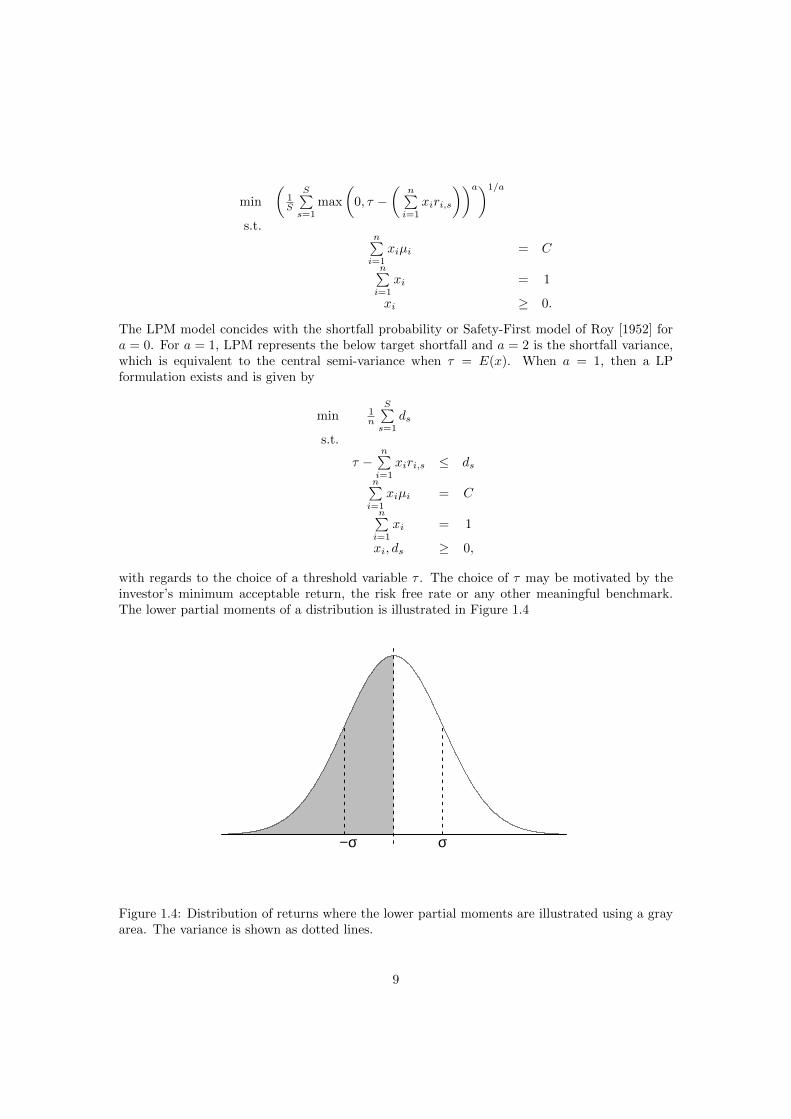
The LPM model concides with the shortfall probability or Safety-First model of Roy [1952] fora = 0. For a = 1, LPM represents the below target shortfall and a = 2 is the shortfall variance,which is equivalent to the central semi-variance when τ = E(x). When a = 1, then a LPformulation exists and is given by

min 1n

S∑s=1

ds

s.t.

τ −n∑i=1

xiri,s ≤ dsn∑i=1

xiµi = C

n∑i=1

xi = 1

xi, ds ≥ 0,

with regards to the choice of a threshold variable τ . The choice of τ may be motivated by theinvestor’s minimum acceptable return, the risk free rate or any other meaningful benchmark.The lower partial moments of a distribution is illustrated in Figure 1.4

σ−σ

Figure 1.4: Distribution of returns where the lower partial moments are illustrated using a grayarea. The variance is shown as dotted lines.

9

Conditional Value at Risk

The heart of risk management is the mitigation of losses, and especially the severe ones whichcan potentially put the entire invested capital at risk. Conditional Value-at-Risk quantifies thelosses in the tail of a distribution as mean shortfall at a specified confidence level [Rockafellar andUryasev, 2002]. In the case of continuous distributions, CVaR is known also as Expected tail loss(ETL), Mean Shortfall [Mausser and Rosen, 1999], or Tail Value-at-Risk [Artzner et al., 1999].CVaR is proposed in the literature as a superior alternative to the industry standard Value-at-Risk (VaR) by conditioning on the losses in excess of VaR, hereby deriving a more appropriateestimation of the significant losses than VaR, i.e. for the confidence level α, the CV aRα isdefined as the mean of the worst (1-α)·100% scenarios. Furthermore, it is consistent with secondorder stochastic dominance shown by Ogryczak and Ruszczynski [2002]. In case of a discretizedstate space it leads to LP solvable portfolio optimization models [Rockafellar and Uryasev, 2002],and in the limited settings where VaR computations are tractable, i.e., for normal and ellipticaldistributions, CVaR maintains consistency with VaR by yielding an identical solution [Keatinget al., 2001]. CVaR can be defined as

CV aRα(X) = ETLα = E(−X| −X > V aRα(X)), (1.5)

where V aRα(X) is defined as V aRα(X) = infx ∈ R : P (X ≤ x) ≥ α. In the discrete setting,CVaR may be adressed using the following model

min ξα +1

Sα

S∑s=1

y+s

s.t. −n∑i=1

xiri,s − ξα ≤ y+s

n∑i=1

xiµi = C

n∑i=1

xi = 1

xi, y+s ≥ 0,

(1.6)

where y+s is an auxiliary variable used for the linearization of the CVaR formulation and ξα isthe Value-at-Risk. The Conditional Value at Risk for a distribution is illustrated in Figure 1.5.

Conditional Drawdown at Risk

Conditional Drawdown at Risk (CDaR) extends the idea of CVaR and conditions on the α worstdrawdowns over a path of cumulative returns. Here, a drawdown is measured on the cumulativereturns of a portfolio rule from the time a decline begins to when a new high is reached, and isillustrated in Figure 1.6. This measure is strongly path dependant, which becomes a problematicfeature as there does not exist a closed form solution for the distribution of this measure with theexception of a Brownian motion with zero drift [see Douady et al., 2000]. Following Chekhlovet al. [2005], the problem may be posed as the following LP

10

σ−σ

VaR

CVaR

Figure 1.5: Distribution of returns where the α worst scenarios constituting CVaR is illustratedusing a gray area. The variance is shown as dotted lines.

min v + 1Sα

S∑s=1

zs

s.t. zs − us + v ≥ 0n∑i=1

xiri,s + us − us−1 ≥ 0

u0 = 0n∑i=1

xiµi = C

n∑i=1

xi = 1

xi, zs, ui ≥ 0,

(1.7)

where z is an auxiliary vector of variables of the conditional drawdowns, u the auxiliary vector ofvariables to model the cumulative returns and v represents the Drawdown at Risk at the quantilelevel α.

1.2.2 Coherency

Irrespective of the type of risk measure, the general reward-risk approach has proven popularboth academically and in the industry as it enables preferences to be summarized in a fewscalar parameters, e.g. mean and variance of returns. Formal qualifications of properties of riskmeasures were first defined in the seminal papers by Artzner et al. [1999] on risk and Rockafellaret al. [2006] on deviation, where the latter established the connection between the two.

Consider the probability space Ω, δ, P , where P is the probability on the δ measurable subsetsof Ω. Rockafellar et al. [2006] define a set of axioms, which are fulfilled in the linear space L2, thatdeviation measures should satisfy. Artzner et al. [1999] provide equivalent ’coherent’ risk measurefunctionals (δ : L2Ω) → (−∞,∞] and argue that the following axioms should be satisfied:

1. δ(C) = −C ∀ constants C

11

2006 2008 2010 2012

6080

100

120

Drawdown

Figure 1.6: Cumulative returns where the maximum drawdown is illustrated as a vertical dashedline between a peak and the subsequent.

2. δ(λX) = λδ(X) ∀ X and λ > 0

3. δ(X +X ′) ≤ δ(X) + δ(X ′) ∀ X and X ′

4. δ(X) ≤ δ(X ′) whenever X ≥ X ′,

where 1. is the translation invariance property, 2. is positive homogeneity, 3. subadditivityproperty and 4. the monotonicity property. More concrete, 1. implies that adding a constant toa set of losses does not change the risk, 2. that holdings and risk scale by the same linear factor,3. that portfolio risk cannot be more than the combined risks of the individual positions, and 4.that larger losses equate to larger risks. The different presented risk measures do not all satisfythe defined properties, and their characteristics are summarized below.

Variance S.D. MAD MiniMax CVaR CDaR LPMτ = c LPMτ = µScaling TRUE TRUE TRUE TRUE TRUE TRUE TRUE TRUELocation 1 TRUE TRUE TRUE FALSE FALSE FALSE FALSE FALSELocation 2 FALSE FALSE FALSE TRUE TRUE FALSE TRUE TRUESubadditivity FALSE TRUE TRUE TRUE TRUE TRUE FALSE TRUE

The four axioms refer to

1. Scaling f(bX) = 1bf(X)

2. Location 1 f(a+X) = f(X)

3. Location 2 f(a+X) = f(X) + a

4. Subadditivity f(X1) + f(X2) ≥ f(X1 +X2),

where f is some risk measure, b a positive scalar and a some constant ∈ R . The scaling propertyis shared by all measures, being a feature of their underlying constituent functions. Variance,S.D., and MAD are location invariant (Location 1) as they are all deviation measures, meaning

12

that they are calculated after centering. Variance is not subadditive, as the square function isknown to be superadditive, contrary to standard deviation which subadditive. CVaR, CDaR,and LPM are not deviation measures and are therefor not location invariant, but do have locationproperty (Location 2), with the exception of CDaR which is path dependent. Interestingly, LPMis subadditiv only when the threshold is equal to the mean of the expected returns [see Broganand Stidham Jr, 2005].

1.2.3 Optimal Financial Portfolios

The bi-objective decision process optimizing the expected return and risk can take advantage ofthe convexity of the efficient frontier to perform a trade-off analysis between the two consideredmatters. Having assumed a trade-off coefficient λ between the risk and the mean, also called therisk aversion coefficient, one may directly compute and evaluate the function µ(x) − λδ(x) andfind the optimal portfolio by solving the following problem:

max(1− λ)µ(x)− λδ(x). (1.8)

Recursively increasing the value of the parameter λ ∈ [0, 1] allows for the generation of a seriesof optimal portfolios for different levels of risk aversion which overall span the efficient frontier.In the context of mean-variance modeling, the technique was introduced by Markowitz [1959] asthe so-called critical line approach. Due to convexity of a given risk measure δ(x) with respectto x, λ ≥ 0 provides a parameterization of the entire set of the µ/δ-efficient portfolios. Hence,the bounded trade-off 0 ≥ λ ≥ 1 in the Markowitz-type mean risk model corresponds to thecomplete weighting parameterization of the model. An alternative approach looks for a riskyportfolio offering the maximum increase of the mean return with respect to a risk-free investmentopportunity. Namely, having given the risk-free rate of return rf one seeks a risky portfolio xthat maximizes the ratio (µ(x) − rf )/δ(x). This leads us to the following ratio optimizationproblem:

maxµ(x)− rfδ(x)

. (1.9)

This particular problem bears special importance when considering the classical Tobin’s two-fund separation theorem [see Tobin, 1958]. The optimal solution of the problem is usually referredto as the tangency portfolio or the market portfolio and coincides with the maximization of theSharpe ratio [Sharpe, 1966], where the Capital Market Line (CML) is a line drawn from theintercept corresponding to rf and that passes tangent to the mean-risk efficient frontier. Anypoint on this line provides the maximum return for each level of risk. The tangency portfoliois the portfolio of risky assets corresponding to the point where the CML is tangent to the ef-ficient frontier. Unfortunately, no analytical solution exists for this problem when bounded bya set of constraints, and one would have to use non-linear optimization or to solve the problemmany times for different λ values in order to find the tangency portfolio. Though, in the spe-cial case where µ and δ are LP computable measures (the efficient frontier is continuous andnon-decreasing), then the original non-linear problem can be transformed into a correspondinglinear one using fractional programming [see Mansini et al., 2003, Stoyanov et al., 2007]. Thisenables the computation of the optimal risk-return portfolio by solving a single linear model, andfurthermore provides the means for adding additional features in the constraints. The generalformulation can be defined as

13

maxn∑i=1

xiµi − τrfs.t. δ(xiri,s − τrf ) ≤ 1

n∑i=1

xi = τ

xi ≥ 0,

(1.10)

where δ is some risk function evaluated on the scenario returns ri,s. µ is the expected returnsfor asset i and scenario s, and τ is an auxiliary scaling variable introduced as part of the linear-fractional programming approach. The optimal solution for the original decision space can beobtained by dividing the optimal portfolio x∗i with the scaling variable τ , i.e. wi = x∗i /τ .

1.3 Thesis Structure

This dissertation is organized around three papers where each addresses different aspects relatedto tactical portfolio optimization and provides novel contributions to the literature.

Chapter 2: Feature Selection for Portfolio Optimization

This paper addresses the problem and impact of parameter uncertainty related to asset allo-cation decisions. Most portfolio selection rules rely on parameters based on sample estimatesfrom historic data. However, the mean-variance model has been shown to perform poorly out-of-sample when using sample estimates of the mean and covariance matrix from historic returns.Moreover, there is a growing body of evidence that such optimization rules are not able to beatsimple rules of thumb, such as 1/N [see DeMiguel et al., 2009, for an overview]. A major causefor these findings has been attributed to uncertainty in the estimated parameters. A strand ofliterature addresses this problem by improving the parameter estimation and/or by relying onmore robust portfolio selection methods. In this paper, we propose a method for reducing theasset menu as a preprocessing stage for the portfolio selection, hereby mitigating the problem ofparameter uncertainty to fewer parameters. The feature selection method works independentlyof the chosen portfolio selection rule, and can therefore be applied to any type of systematicrisk averse asset allocation. We show that we are able to preserve most of the diversificationbenefits from the original asset universe, while alleviating the parameter estimation problem. Tofurther emphasize these findings, we conduct out-of-sample back tests to show that in most casesdifferent well-established portfolio selection rules applied on the reduced asset universe are ableto improve alpha relative to different prominent factor models.

Novel contribution: The paper makes four contributions to the literature on clustering inportfolio optimization. First, our out-of-sample back tests are based on long and well-knowntime series. Specifically, we use the value weighted 49 industry portfolios provided by KennethFrench as well as the constituting stocks of the S&P 500. For both data sets, we use monthlyreturns from 1970 to 2013. Second, in addition to the classical minimum-variance portfolio andthe tangency portfolio, we consider also the more advanced portfolio selection rules suggested byKan and Zhou [2007] and Tu and Zhou [2011]. We compare pairwise the results with and withoutfeature selection. Noteworthy, the application of feature selection allows the use of these portfolioselection rules on data sets with more assets than observations. Third, in line with Kritzmanet al. [2010] we highlight the importance of the length of the observation period by presentingback test results for rolling windows of 5, 10, 15 and 20 years. Finally, we base our assessment onthe alpha relative to the most prominent factor models, such as CAPM, the Fama-French Three

14

Factor model, and the Fama-French-Carhart Four Factor model. As a main result, we show thatfor most test cases the performance of the reduced asset universe improves. In particular, weshow that the alpha of the equal weight (1/N) strategy also benefits from reducing the assetmenu.

Chapter 3: Portfolio Selection under Supply Chain Predictability

The second paper investigates the existence of cross-industry predictability of returns throughan econometric study. Using empirical data, we analyze whether lagged returns of stocks fromone industry predict those of another in the same market. The hypothesis takes its origin in theworks of Shiller and Sims, who both argue that investors are subject to an attention span whichhas the implication that not all information is incorporated in the market instantaneously, butwith a time lag. Our hypothesis is that industries are related through the supply-chain but donot immediately share information with each other. This predicament gives rise to return pre-dictability. We analyse this question through a VAR process and find downstream predictabilityin the supply chain along with autocorrelation. Furthermore, we address the economic relevanceof this finding in an out-of-sample portfolio setting where we assign weights according to themaximization of the STAR ratio [see Martin et al., 2003]. The STAR ratio is equivalent to theSharpe ratio where the risk function is evaluated in terms of Conditional Value at Risk. Wecompare the results of estimating expected returns using a VAR process and a Brownian motion.The latter is used to eliminate the effect of predictability. We find that the cross-industry pre-dictability of returns, in addition to being statistically significant, is also economically relevant,which amounts to significant out-of-sample excess returns, and a noteworthy increase in Sharperatio.

Novel contribution: We show in this paper that some industries tend to drive the returnsof others, which results in return predictability. Our contribution to the literature is twofold,but can overall be summarized as rigorous analysis of the magnitude of the predictive behaviorof certain industry segments on the supply chain across the U.S. economy. First, we provide anon-parametric mapping of the significant relations between different industry segments in orderto uncover lead and lagged returns on a monthly basis using a VAR process. Second, we analysethe predictability in an out-of-sample portfolio selection setting to test if the predictability iseconomically significant. Here, we optimize a portfolio according to the STAR ratio. We comparethe results based on a vector autoregressive process to that of using a Brownian motion forestimating expected returns, and show that our hypothesis holds true both in-sample and out-of-sample.

Chapter 4: Portfolio Optimization of Commodity Futures with SeasonalComponents and Higher Moments

The third paper addresses the implication of including commodities in a traditional well-diversifiedequity portfolio. The literature suggests that there exist in-sample diversification benefits ofincluding commodities in portfolio optimization, but that these benefits are not preserved out-of-sample. We provide an extensive in-sample study of the seasonality in returns, risk-returnprofiles and diversification characteristics of a broad range of different commodity futures. Wefind that there exists statistical significant evidence of seasonality, and hereby predictability, inthe considered non-metal commodities and gold. We address the same setting in an out-of-sampleanalysis by constructing portfolios of ten commodities and a stock index using the classical tan-gency mean-variance model and the maximum Omega ratio model. The Omega ratio is the ratio

15

between the first order upper and lower partial moments. We suggest using Shieve bootstrap-ping for the estimation of the expected return and risk functions to control for the seasonality.We show that the predictability in commodity returns should be considered, and leads to sig-nificant excess return and increase in Sharpe ratio. Furthermore, our results confirm the poorout-of-sample performance of including commodities in a well-diversified equity portfolio, whenseasonality is not considered.

Novel contribution: This paper adds to the existing literature on the role of commodities inportfolio optimization. We identify four novel contributions in this paper. First, we analyze alarge basket of commodities over a longer time horizon than usually presented in the literature(1975.01 - 2014.12). Second, we provide a rigorous analysis of the empirical distribution of theSharpe ratio of various commodity futures along with the impact of seasonality in commodityreturns on the allocation of assets in an in-sample mean-variance setting. Thirdly, we proposeto use the Omega ratio in portfolio optimization of commodities in order to account for higherorder statistical moments. Fourthly, we confirm that the mean-variance model performs poorlyout-of-sample for optimizing a basket of commodities when using sample estimates, and provideevidence that a main course for this result is the negligence of seasonality in the parameterestimation process when appropriate.

Chapter 5: Conclusion

Finally, I summarize my findings, conclude, and gives directions towards future research.

16

Bibliography

Bahram Adrangi, Arjun Chatrath, Kanwalroop Kathy Dhanda, and Kambiz Raffiee. Chaos inoil prices? Evidence from futures markets. Energy Economics, 23(4):405–425, 2001.

Ronald W Anderson. Some determinants of the volatility of futures prices. Journal of FuturesMarkets, 5(3):331–348, 1985.

Robert D Arnott and Frank J Fabozzi. Asset allocation: A handbook of portfolio policies, strate-gies & tactics. Probus Professional Pub, 1988.

Philippe Artzner, Freddy Delbaen, Jean-Marc Eber, and David Heath. Coherent measures ofrisk. Mathematical Finance, 9(3):203–228, 1999.

Doron Avramov. Stock return predictability and asset pricing models. Review of FinancialStudies, 17(3):699–738, 2004.

Doron Avramov and Russ Wermers. Investing in mutual funds when returns are predictable.Journal of Financial Economics, 81(2):339–377, 2006.

Vijay S Bawa. Safety-first, stochastic dominance, and optimal portfolio choice. Journal ofFinancial and Quantitative Analysis, 13(02):255–271, 1978.

Vijay S Bawa and Eric B Lindenberg. Capital market equilibrium in a mean-lower partial momentframework. Journal of Financial Economics, 5(2):189–200, 1977.

Geert Bekaert and Robert J Hodrick. Characterizing predictable components in excess returnson equity and foreign exchange markets. The Journal of Finance, 47(2):467–509, 1992.

Daniel Bernoulli. Exposition of a new theory on the measurement of risk. Econometrica: Journalof the Econometric Society, pages 23–36, 1954.

Dimitris Bertsimas and Angela King. Or foruman algorithmic approach to linear regression.Operations Research, 64(1):2–16, 2015.

Stephen P Bradley and Dwight B Crane. A dynamic model for bond portfolio management.Management Science, 19(2):139–151, 1972.

Anita J Brogan and Shaler Stidham Jr. A note on separation in mean-lower-partial-momentportfolio optimization with fixed and moving targets. Iie Transactions, 37(10):901–906, 2005.

Stephen PA Brown and Mine K Yucel. What drives natural gas prices? The Energy Journal,pages 45–60, 2008.

John Y Campbell. Stock returns and the term structure. Journal of Financial Economics, 18(2):373–399, 1987.

17

John Y Campbell, Yeung Lewis Chan, and Luis M Viceira. A multivariate model of strategicasset allocation. Journal of Financial Economics, 67(1):41–80, 2003.

David R Carino, Terry Kent, David H Myers, Celine Stacy, Mike Sylvanus, Andrew L Turner,Kouji Watanabe, and William T Ziemba. The russell-yasuda kasai model: An asset/liabilitymodel for a japanese insurance company using multistage stochastic programming. Interfaces,24(1):29–49, 1994.

Alexei Chekhlov, Stanislav Uryasev, and Michael Zabarankin. Drawdown measure in portfoliooptimization. International Journal of Theoretical and Applied Finance, 8(01):13–58, 2005.

John H Cochrane. State-space vs. var models for stock returns. Unpublished manuscript, 2008.

Giorgio Consigli and MAH Dempster. Dynamic stochastic programmingfor asset-liability man-agement. Annals of Operations Research, 81:131–162, 1998.

Andrea Consiglio, Flavio Cocco, and Stavros A Zenios. The value of integrative risk managementfor insurance products with guarantees. The Journal of Risk Finance, 2(3):6–16, 2001.

David M Cutler, James M Poterba, and Lawrence H Summers. Speculative dynamics. TheReview of Economic Studies, 58(3):529–546, 1991.

Thomas Dangl and Michael Halling. Predictive regressions with time-varying coefficients. Journalof Financial Economics, 106(1):157–181, 2012.

Victor DeMiguel, Lorenzo Garlappi, and Raman Uppal. Optimal versus naive diversification:How inefficient is the 1/n portfolio strategy? Review of Financial Studies, 22(5):1915–1953,2009.

Raphael Douady, AN Shiryaev, and Marc Yor. On probability characteristics of” downfalls” ina standard brownian motion. Theory of Probability & Its Applications, 44(1):29–38, 2000.

Eugene F Fama and Kenneth R French. Commodity futures prices: Some evidence on forecastpower, premiums, and the theory of storage. Journal of Business, pages 55–73, 1987.

Eugene F Fama and Kenneth R French. Dividend yields and expected stock returns. Journal ofFinancial Economics, 22(1):3–25, 1988.

Eugene F Fama and Kenneth R French. Business conditions and expected returns on stocks andbonds. Journal of Financial Economics, 25(1):23–49, 1989.

Miguel A Ferreira and Pedro Santa-Clara. Forecasting stock market returns: The sum of theparts is more than the whole. Journal of Financial Economics, 100(3):514–537, 2011.

Wayne E Ferson and Campbell R Harvey. The risk and predictability of international equityreturns. Review of Financial Studies, 6(3):527–566, 1993.

Wayne E Ferson, Campbell R Harvey, et al. The variation of economic risk premiums. Journalof Political Economy, 99(2):385–415, 1991.

Peter C Fishburn. Mean-risk analysis with risk associated with below-target returns. TheAmerican Economic Review, 67(2):116–126, 1977.

Alois Geyer, Michael Hanke, and Alex Weissensteiner. Scenario tree generation and multi-assetfinancial optimization problems. Operations Research Letters, 41(5):494–498, 2013.

18

Itzhak Gilboa and David Schmeidler. Maxmin expected utility with non-unique prior. Journalof mathematical economics, 18(2):141–153, 1989.

Bennett Golub, Martin Holmer, Raymond McKendall, Lawrence Pohlman, and Stavros A Zenios.A stochastic programming model for money management. European Journal of OperationalResearch, 85(2):282–296, 1995.

Giora Hanoch and Haim Levy. The efficiency analysis of choices involving risk. The Review ofEconomic Studies, 36(3):335–346, 1969.

Sam James Henkel, J Spencer Martin, and Federico Nardari. Time-varying short-horizon pre-dictability. Journal of Financial Economics, 99(3):560–580, 2011.

Erik Hjalmarsson. Predicting global stock returns. Journal of Financial and Quantitative Anal-ysis, 45(1):49–80, 2010.

Raymond Kan and Guofu Zhou. Optimal portfolio choice with parameter uncertainty. Journalof Financial and Quantitative Analysis, 42(03):621–656, 2007.

Michal Kaut and Stein W Wallace. Evaluation of scenario-generation methods for stochasticprogramming. Pacific Journal of Optimization, 3:257–271, 2003.

Con Keating, Hyun Song Shin, Charles Goodhart, Jon Danielsson, et al. An academic responseto basel II. Technical report, Financial Markets Group, 2001.

David Kenyon, Kenneth Kling, Jim Jordan, William Seale, and Nancy McCabe. Factors affectingagricultural futures price variance. Journal of Futures Markets, 7(1):73–91, 1987.

Hiroshi Konno and Hiroaki Yamazaki. Mean-absolute deviation portfolio optimization modeland its applications to tokyo stock market. Management science, 37(5):519–531, 1991.

Hiroshi Konno, Hiroshi Shirakawa, and Hiroaki Yamazaki. A mean-absolute deviation-skewnessportfolio optimization model. Annals of Operations Research, 45(1):205–220, 1993.

Mark Kritzman, Sebastien Page, and David Turkington. In defense of optimization: the fallacyof 1/n. Financial Analysts Journal, 66(2):31–39, 2010.

Martin I Kusy and William T Ziemba. A bank asset and liability management model. OperationsResearch, 34(3):356–376, 1986.

Renata Mansini, W lodzimierz Ogryczak, and M Grazia Speranza. Lp solvable models for portfoliooptimization: A classification and computational comparison. IMA Journal of ManagementMathematics, 14(3):187–220, 2003.

Harry Markowitz. Portfolio selection. The journal of finance, 7(1):77–91, 1952.

Harry Markowitz. Portfolio selection: Efficient diversification of investments. cowles foundationmonograph no. 16, 1959.

R Douglas Martin, Svetlozar Zari Rachev, and Frederic Siboulet. Phi-alpha optimal portfoliosand extreme risk management. The Best of Wilmott 1: Incorporating the Quantitative FinanceReview, 1:223, 2003.

Helmut Mausser and Dan Rosen. Beyond var: From measuring risk to managing risk. In Compu-tational Intelligence for Financial Engineering, 1999.(CIFEr) Proceedings of the IEEE/IAFE1999 Conference on, pages 163–178. IEEE, 1999.

19

Nikolaos Milonas and Ashok Vora. Sources of non-stationarity in cash and futures prices. Reviewof Research in Futures Markets, 4(3):314–326, 1985.

John M Mulvey and Hercules Vladimirou. Stochastic network programming for financial planningproblems. Management Science, 38(11):1642–1664, 1992.

Soren S Nielsen and Stavros A Zenios. A stochastic programming model for funding singlepremium deferred annuities. Mathematical Programming, 75(2):177–200, 1996.

Wlodzimierz Ogryczak and Andrzej Ruszczynski. Dual stochastic dominance and quantile riskmeasures. International Transactions in Operational Research, 9(5):661–680, 2002.

Lasse Heje Pedersen. Efficiently inefficient: how smart money invests and market prices aredetermined. Princeton University Press, 2015.

Andre F Perold and William F Sharpe. Dynamic strategies for asset allocation. FinancialAnalysts Journal, 51(1):149–160, 1995.

Thomas K Philips, Greg T Rogers, and Robert E Capaldi. Tactical asset allocation: 1977-1994.The Journal of Portfolio Management, 23(1):57–64, 1996.

John Quiggin. A theory of anticipated utility. Journal of Economic Behavior & Organization, 3(4):323–343, 1982.

David E Rapach, Jack K Strauss, and Guofu Zhou. Out-of-sample equity premium prediction:Combination forecasts and links to the real economy. Review of Financial Studies, 23(2):821–862, 2010.

R Tyrrell Rockafellar and Stanislav Uryasev. Conditional value-at-risk for general loss distribu-tions. Journal of Banking & Finance, 26(7):1443–1471, 2002.

R Tyrrell Rockafellar, Stan Uryasev, and Michael Zabarankin. Generalized deviations in riskanalysis. Finance and Stochastics, 10(1):51–74, 2006.

Richard Roll. Orange juice and weather. The American Economic Review, 74(5):861–880, 1984.

Andrew D Roy. Safety-first and the holding of assets. Economctrica, 20(3):431–449, 1952.

William F Sharpe. Mutual fund performance. The Journal of business, 39(1):119–138, 1966.

William F Sharpe. A linear programming approximation for the general portfolio analysis prob-lem. Journal of Financial and Quantitative Analysis, 6(05):1263–1275, 1971a.

William F Sharpe. Mean-absolute-deviation characteristic lines for securities and portfolios.Management Science, 18(2):B–1, 1971b.

William F Sharpe. Asset allocation: Management style and performance measurement. TheJournal of Portfolio Management, 18(2):7–19, 1992.

Bruno Solnik. The performance of international asset allocation strategies using conditioninginformation. Journal of Empirical Finance, 1(1):33–55, 1993.

M Grazia Speranza. Linear programming models for portfolio optimization. Finance, 14(1):107–123, 1993.

20

Bernell K Stone. A general class of three-parameter risk measures. The Journal of Finance, 28(3):675–685, 1973.

Stoyan V Stoyanov, Svetlozar T Rachev, and Frank J Fabozzi. Optimal financial portfolios.Applied Mathematical Finance, 14(5):401–436, 2007.

James Tobin. Liquidity preference as behavior towards risk. The review of economic studies, 25(2):65–86, 1958.

Jun Tu and Guofu Zhou. Markowitz meets talmud: A combination of sophisticated and naivediversification strategies. Journal of Financial Economics, 99(1):204–215, 2011.

John Von Neumann and Oskar Morgenstern. Theory of games and economic behavior. Bull.Amer. Math. Soc, 51(7):498–504, 1945.

Eric J Weigel. The performance of tactical asset allocation. Financial Analysts Journal, 47(5):63–70, 1991.

Shlomo Yitzhaki. Stochastic dominance, mean variance, and gini’s mean difference. The Amer-ican Economic Review, 72(1):178–185, 1982.

Martin R Young. A minimax portfolio selection rule with linear programming solution. Man-agement science, 44(5):673–683, 1998.

Lotfi A Zadeh. Fuzzy sets. Information and control, 8(3):338–353, 1965.

21

Chapter 2

Feature Selection for PortfolioOptimizationThomas Trier Bjerring · Omri Ross · Alex Weissensteiner

Status: Accepted, Annals of Operations Research

Abstract: Most portfolio selection rules based on the sample mean and co-variance matrix perform poorly out-of-sample. Moreover, there is a growingbody of evidence that such optimization rules are not able to beat simple rulesof thumb, such as 1/N. Parameter uncertainty has been identified as one ma-jor reason for these findings. A strand of literature addresses this problem byimproving the parameter estimation and/or by relying on more robust port-folio selection methods. Independent of the chosen portfolio selection rule, wepropose using feature selection first in order to reduce the asset menu. Whilemost of the diversification benefits are preserved, the parameter estimationproblem is alleviated. We conduct out-of-sample back-tests to show that inmost cases different well-established portfolio selection rules applied on the re-duced asset universe are able to improve alpha relative to different prominentfactor models.

Keywords: Portfolio Optimization, Parameter Uncertainty, Feature Selec-tion, Agglomerative Hierarchical Clustering

2.1 Introduction

The seminal work of Markowitz [1952] has inspired a lot of work in the field of asset allocation.However, the solutions obtained by such techniques are usually very sensitive to the input pa-rameters [see e.g. Best and Grauer, 1991] with the consequence that estimation errors lead tounstable and extreme positions in single assets. Chopra and Ziemba [2011] are one of the first toquantify the consequences of misspecified parameters in asset allocation decisions. Specifically,they illustrate that in their setting errors in expected returns are about ten times more importantthan errors in variances and covariances. Furthermore, in addition to the general consensus thatexpected returns are notoriously difficult to predict, Merton [1980] shows that even if the true pa-rameters were constant, very long time series would be required to estimate expected returns in areliable way. As a consequence, a trading strategy based on the sample minimum variance port-

23

folio, which completely abstains from estimating expected returns, shows a better risk-adjustedperformance than many other portfolio selection rules [see e.g. Haugen and Baker, 1991, Clarkeet al., 2006, Scherer, 2011]. Others propose different techniques to alleviate the problem of esti-mating expected returns. Jorion [1986] considers explicitly the potential utility loss when usingsample means to estimate expected returns. In order to minimize this loss function, he usesBayes-Stein estimation to shrink the sample means toward a common value. A simulation studyshows that this correction provides significant gains. Black and Litterman [1992] argue that theonly sensible “neutral” expected returns are those that would clear the market if all investorshad identical views. Hence, the natural choice are the equilibrium expected returns derived fromreverse optimization using the current market capitalization. Having these “neutral expectedreturns” as a starting point, they illustrate how to combine them with an investor’s own view ina statistically consistent way.

Kan and Zhou [2007] show that there is a very significant interactive effect between theestimation of the parameters and the ratio of the number of assets to the number of observations.If the number of assets is small compared to the number of observations, then the estimationof expected returns is more important [in line with Chopra and Ziemba, 2011]. However, whenthis fraction grows, then estimation errors in the sample covariance grow too, and may becomemore severe in terms of utility costs than the estimation errors in expected returns. Furthermore,when the number of assets exceeds the number of observations, the sample covariance matrix isalways singular (even if the true covariance matrix is known to be non-singular). Many papersaddress the problem of estimating the covariance matrix from limited sample data.

Ledoit and Wolf [2003a, 2004, 2003b], Ledoit et al. [2012] propose using the “shrinkage”technique in order to pull extreme coefficients in the sample covariance matrix, which tendto contain a lot of error, towards more central values of a highly structured estimator. Theyderive the optimal shrinkage intensity in terms of a loss function, and they suggest using factormodels1 or constant correlation models as structured estimators. Given that weight constraintsimprove the performance of mean-variance efficient portfolios, Jagannathan and Ma [2003] studythe short-sale constrained minimum-variance portfolio. They show that the optimal solutionunder short-sale constraints corresponds to the optimal solution of the unconstrained problemif shrinkage is used to estimate the covariance matrix, i.e. there is a one-to-one relationshipbetween short-sale constraints and the shrinkage technique. DeMiguel et al. [2009a] generalizethese results by solving the classical minimum-variance problem under norm-constrained assetweights. They show that their setting nests the shrinkage technique of Ledoit and Wolf [2003a,2004] and Jagannathan and Ma [2003] as special cases. Given that for more volatile stocks theparameter estimation risk is higher, Levy and Levy [2014] propose two variance-based constraintsto alleviate the problem of parameter uncertainty. First, the Variance-Based Constraints on thesingle weights, which are inversely proportional to the sample standard deviation of each asset.Second, the Global Variance-Based Constraints, where instead of sharp boundary constraintson each stock a quadratic “cost” is assigned to deviations from an equally weighted portfolio.Comparing ten optimization methods, they find that the two new suggested methods typicallyyield the best performance in terms of Sharpe ratio.

Another method to mitigate the estimation problem uses more portfolios than those proposedby the classical two-funds Tobin separation theorem. Kan and Zhou [2007] suggest adding athird risky fund to the risk-free asset and to the sample tangency portfolio to hedge againstparameter uncertainty. In particular, under the assumption of constant parameters, they showthat a portfolio which optimally combines the risk-free asset, the sample tangency portfolio (TP)and the sample global minimum-variance portfolio (MVP) dominates a portfolio with just therisk-free asset and the sample tangency portfolio.

1See Kritzman [1993] who compares factor analysis and cross-sectional regression for that purpose.

24

The most extreme approach to address the problem of parameter uncertainty is to ignore allhistorical observations and to invest equally in the available assets. Such a strategy is known asthe 1/N rule. Duchin and Levy [2009] use the 30 Fama-French industry portfolios (2001–2007)to compare the 1/N rule against a Markowitz mean-variance rule under short-sale constraints.They illustrate that for a low number of assets (below 25) the 1/N rule provides a higher averageout-of-sample return. Only if all 30 assets are traded, then the classical optimization approachoutperforms the 1/N rule slightly. DeMiguel et al. [2009b] compare 14 portfolio selection rulesacross seven empirical datasets and show that none is consistently better out-of-sample thanthe 1/N rule. Furthermore, under the assumption of constant parameters, they show that time-series of extreme length (more than 6000 months for 50 assets) are necessary to beat the 1/Nbenchmark.

Given the results of DeMiguel et al. [2009b], Tu and Zhou [2011] combine the 1/N rulewith four other well-known portfolio selection rules. Among others, they extend the Kan andZhou [2007] model and propose adding the equally weighted 1/N portfolio as a fourth fund inan optimal way to reduce the estimation error. The MVP and the 1/N portfolio are naturalcandidates: While the MVP does not depend on expected returns, for the 1/N portfolio neitherexpected returns nor a covariance matrix have to be estimated.2

The results given by DeMiguel et al. [2009b] raise serious concerns about portfolio optimiza-tion altogether. In defense of optimization, Kritzman et al. [2010] argue that most studies rely ontoo short samples for estimating expected returns, which often yields implausible results. Theyshow that when estimations of expected excess returns are based on long-term samples, thenusually optimized portfolios outperform equally weighted portfolios.

To sum up: Many of the aforementioned papers illustrate that the problem of parameteruncertainty increases with the number of assets [see e.g. Kan and Zhou, 2007]. Different datamining techniques such as factor models [see e.g. Kritzman, 1993], shrinkage of the mean [seee.g. Jorion, 1986] and shrinkage of the covariance [see e.g. Ledoit and Wolf, 2003a, 2004] areproposed to alleviate the problem of the parameter estimation. Under the assumption of con-stant parameters, extending the observation period improves the performance of optimizationbased portfolio rules [see e.g. DeMiguel et al., 2009b, Kritzman et al., 2010]. However, whetherparameters are really constant over time is questionable, which suggests that simply expandingthe observation period might not be the best strategy in practice.

Compared to the above mentioned literature, in this paper we propose using feature selec-tion by agglomerative hierarchical clustering. Based on correlation, we create groups of assetssuch that the similarity within a cluster and the dissimilarity between different clusters is max-imized. From each group we select then one representative asset to construct a smaller but yetcomprehensive enough universe.3 As the representative asset we use the medoid, whose averagedissimilarity to all the objects in the cluster is minimal. While the reduced asset menu facilitatesthe estimation of the parameters, the chosen assets still allow to benefit from diversification. Ourchoice is motivated by previous studies. Tola et al. [2008] show that clustering algorithms canimprove the reliability of the portfolio in terms of the ratio between predicted and realized risk.Lisi and Corazza [2008] use clustering for a practical portfolio optimization task under cardi-nality constraints. They use different distance functions and illustrate that in general clusteringimproves the out-of-sample performance compared to a benchmark. Nanda et al. [2010] comparedifferent clustering techniques (as K-means, Fuzzy C-means, Self Organizing Maps) for portfoliomanagement in the Indian market and report benefits compared to the benchmark (the Sensexindex).

2For the rest of the paper, when referring to the Tu and Zhou [2011] strategy, we mean the optimal combinationof 1/N with Kan and Zhou [2007].

3In the following we use the term “feature selection” as synonym for “hierarchical clustering”.

25

The present work makes four contributions to the literature on clustering in portfolio op-timization. First, compared to the above mentioned papers, our out-of-sample back-tests arebased on long and well-known time series. Specifically, we use the value-weighted 49 industryportfolios provided by Kenneth French4 as well as the constituent stocks of the S&P 500. Forboth data sets, we use monthly returns from 1970 to 2013. Second, in addition to the classi-cal minimum-variance portfolio and the tangency portfolio, we consider also the more advancedportfolio selection rules suggested by Kan and Zhou [2007] and Tu and Zhou [2011]. We comparepairwise the results with and without feature selection.5 Furthermore, feature selection allows touse these portfolio selection rules also on data sets with more assets than observations. Third,in line with Kritzman et al. [2010] we highlight the importance of the length of the observationperiod by presenting back-test results for rolling windows of 5, 10, 15 and 20 years. Finally, webase our assessment on the alpha relative to the most prominent factor models, such as Famaand French [1993] and Carhart [1997]. As a main result, we show that for most test cases theperformance of the reduced asset universe improves. In particular, we show that the alpha ofthe 1/N strategy also benefits from reducing the asset menu. As the 1/N rule is not prone toparameter estimation errors, this result might be counterintuitive. We explain this finding withother beneficial properties of feature selection. First, in addition to alleviating the problems dueto parameter estimation, the concentration risk of a portfolio is also reduced. To illustrate thispoint, consider the fact that over 20% of the stocks in the S&P 500 are from the technologysector. As a result, the 1/N portfolio has high concentration risk in this sector. Feature selectionforms groups such that the intra-group similarity and the inter-group dissimilarity is maximized,i.e. similar stocks are allocated to the same group. By choosing then a representative asset out ofeach group such sector-concentration risks are mitigated. Second, we show that for appropriateobservation periods feature selection reduces the beta of the 1/N portfolio, which relates to the“betting-against-beta” idea proposed by Frazzini and Pedersen [2014].

The paper is structured as follows. Section 2 summarizes the classical portfolio optimizationtechniques which are used in this paper. Section 3 offers a more detailed explanation of how weuse feature selection for the problem at hand. Section 4 describes the data and the results ofusing feature selection in practice, and Section 5 concludes.

2.2 Classical Mean-Variance Optimization

Portfolio selection according to Markowitz is based on the assumption of multivariate normalasset returns. An investor, faced with the decision on how to allocate funds to N risky and oneriskless asset, optimizes the trade-off between the expectation and the variance of the portfolioreturns. This preference can be formulated as

maxw

wᵀµ− λ

2wᵀΣw,

where w = (w1, ..., wi, ..., wN )ᵀ represents the weights allocated to each risky asset in the portfo-lio, µ is the vector of expected excess returns over the risk free rate, λ denotes the risk aversioncoefficient, and Σ is the variance-covariance matrix. Consequently, the difference 1 − 1ᵀw isinvested in the riskless asset.

In practice the parameters µ and Σ are unknown, i.e. the portfolio optimization has to beconducted under parameter uncertainty. Estimation errors can have a substantial influence on

4see http://mba.tuck.dartmouth.edu/pages/faculty/ken.french/data_library.html5Given the focus of this paper, we want to point out that the proposed investigation is not intended as a horse

race between the different portfolio selection rules.

26

the out-of-sample performance of the model, and may lead to solutions that are far away fromthe true optimal portfolios [see DeMiguel and Nogales, 2009]. In order to alleviate parameteruncertainty, Kan and Zhou [2007] propose a three-fund rule, which, in addition to the risk-freeasset and the tangent portfolio, engages a third risky portfolio to hedge against the estimationrisk. Furthermore, Tu and Zhou [2011] extend the three-fund rule and introduce the 1/N portfolioas a fourth portfolio.

DeMiguel et al. [2009b] show with a simulation study that the impact of parameter uncertaintyon the performance of optimized portfolios depends heavily on the number of included assets.Given constant parameters, they illustrate that very long time series are needed to estimate µ andΣ precisely enough to outperform an equally weighted portfolio. In reality, however, parametervalues may vary over time, i.e. simply expanding the estimation window might induce the riskof using outdated observations.

Therefore, instead of simply expanding the window for the parameter estimation, in thispaper we suggest a preliminary screening of the assets considered for optimization to reducethe dimensionality of the parameter estimation problem, and hereby improve the out-of-samplequality of the results.

In order to assess the performance of feature selection, we compare pairwise the results of fivedifferent portfolio rules with and without reduction of the asset universe. More specifically, theseasset allocation rules are the global minimum variance portfolio, the tangency mean-varianceportfolio, the three-fund portfolio, the four-fund portfolio, and the 1/N portfolio. A short pre-sentation of them is provided below.

Global Minimum Variance Portfolio

The minimum variance portfolio is a special case in the mean-variance portfolio framework, wherethe combination of risky assets is chosen such that the total variance of the portfolio returns isminimized, that is

minw

wᵀΣw

s.t. 1ᵀw = 1.

As this rule relies only on the estimation of the covariance matrix of asset returns, and ignores theexpected returns, it is less prone to estimation errors as fewer parameters have to be estimated.Analytically, the weights of the minimum variance portfolio can be expressed as

w∗MV =Σ−11

1ᵀΣ−11. (2.1)

Mean-Variance Tangency Portfolio

Tobin [1958] expands Markowitz’ seminal work for a risk-free asset and shows that the assetallocation task results in maximizing the Sharpe ratio of the portfolio

maxw

wᵀµ√wᵀΣw

s.t. 1ᵀw = 1.

Thereafter, dependent on the investor’s risk aversion, a combination between the resulting tan-gency portfolio and the risk-free asset is chosen. Analytically, the weights of the tangencyportfolio are given by

w∗TP =Σ−1µ

1ᵀΣ−1µ. (2.2)

27

The Three-Fund Rule

If the true mean and covariance of asset returns could be estimated precisely, as assumed intheory, then the two-fund separation would hold perfectly. However, when the parameters areunknown, the tangency portfolio is obtained with estimation errors. Intuitively, by using anadditional risky portfolio the estimation problem can be alleviated. Kan and Zhou [2007] proposeusing the global minimum-variance portfolio as a third fund. As the estimation errors of theminimum variance portfolio and the tangency portfolio are not perfectly correlated, an optimalcombination of them allows to improve the out-of-sample performance. The non-normalizedweights of the combined portfolios are given by

wKZ =c3γ

(cΣ−1µ+ fΣ−11

), (2.3)

where c and f are chosen optimally to maximize the expected utility of a mean-variance investor

given the relative risk aversion parameter γ and the constant scalar c3 = (T−N−1)(T−N−4)T (T−2) . The

allocation of funds to each of the risky portfolios depends on the number of assets N and thelength of the estimation window T . The more severe the parameter estimation problem, thehigher the optimal proportion invested in the global minimum variance portfolio. In line withDeMiguel et al. [2009b], we set γ equal to 1, and we only focus on the composition of the riskypart of the suggested portfolios. More specifically, we calculate the relative weights of the riskyassets by

w∗KZ =wKZ|1ᵀwKZ |

, (2.4)

where |1ᵀwKZ | guarantees that the direction of the portfolio position is preserved in cases wherethe sum of the weights of the risky assets is negative.

The Four-Fund Rule

DeMiguel et al. [2009b] show that the 1/N portfolio rule is difficult to outperform, especially ifthe observation period is short. However, as the 1/N rule makes no use of the sample information,it will fail to converge to the true optimal portfolio (unless, by chance, the two are the same).Therefore, if 1/N is far from the optimal portfolio its performance might be poor. Tu and Zhou[2011] propose the four-fund rule by combining the three fund-rule [see Kan and Zhou, 2007] inan optimal way with the 1/N portfolio. The non-normalized weights of this portfolio combinationrule are

wTZ = (1− δ)we + δwKZ , (2.5)

where we is the equally weighted (1/N) portfolio and wKZ is the (non-normalized) optimalportfolio defined by the three-fund rule. The parameter δ, which defines the ratio of wealthallocated to each of the portfolios, is determined by the number of assets N and the number ofobservations T . The larger the number of assets relative to the number of observations, the moreis invested in the 1/N portfolio, and the suggested portfolio becomes less prone to estimationerrors. As in equation (2.4), we normalize the portfolio weights as

w∗TZ =wTZ|1ᵀwTZ |

. (2.6)

In general, the above mentioned papers assume unknown but constant parameters, which haveto be estimated from historical observations. To mitigate the estimation problem, an increasingnumber of assets N requires more observations T . In the limit – due to the Law of Large Numbers– the estimated parameters converge towards their true values. However, in case of time-varying

28

investment opportunities and/or structural breaks, historical data may not correctly reflect thecurrent state of the markets. On the other hand, for N > T , the sample covariance matrixis always singular. Therefore, it is natural to investigate whether it is beneficial to reduce thesize of the asset menu and apply the portfolio rules to a representative subset, which reflectsthe overall dependence structure. The next section provides a detailed explanation (and a fewexamples) on how to reduce the asset universe using feature selection.

2.3 Dimensionality Reduction Using Feature Selection

This part of the paper proposes a heuristic, namely agglomerative hierarchical clustering, whichexploits the underlying correlation structure of the complete universe in order to reduce the sizeof an N -dimensional asset universe significantly. The starting point for the clustering is thecovariance matrix after shrinkage, for which we rely on a constant correlation matrix (set equalto the sample average) as structured estimator [see Ledoit and Wolf, 2003b].

2.3.1 Heterogeneity of the Asset Universe

In order to benefit from diversification when applying portfolio selection rules, the reduced subsetn ⊂ N should consist of the n assets with the lowest overall correlation with each other. Iden-tifying this sub-space can be translated into the problem of finding the longest path of n ⊂ Nvertices in a simple cycle of an undirected graph. The distance between the vertices can berepresented by di,j = 1− ρi,j , where ρi,j is the correlation between assets i and j. A correlationof 0.8 would then be equal to a Euclidean distance of 0.2, whereas a correlation of –0.2 wouldbe 1.2. Unfortunately, due to the curse of dimensionality, analyzing all subspaces of n ⊂ N isnot a feasible task.6 Furthermore, from an optimization point of view, the challenge of findingthe longest path is a NP-hard problem, i.e. cannot be solved in polynomial time, and generalapproximation techniques are not available.

Therefore, we propose a heuristic method, hierarchical clustering, for decomposing a universeof N assets into n subspaces. We then choose the most representative assets in each subspace,identified as the medoid, in order to preserve the heterogeneity of the original asset universe.The reduction of the asset universe should alleviate the parameter estimation problem.

2.3.2 Hierarchical Clustering

Classification and cluster analysis are used to group a collection of objects into subcategories/subsetsgiven a chosen criterion. In this work, hierarchical clustering is proposed as a method to establishthe relationship between different components in an asset universe.

In general, hierarchical clustering generates a nested sequence of partitions of objects orobservations [see Xu and Wunsch, 2005]. More specifically, we consider agglomerative hierarchicalclustering, which starts by placing each object in its own cluster and then merges these atomicclusters into increasingly larger clusters until all objects are enveloped [see e.g. Tan et al., 2006].Given a set of objects and a clustering criterion, the partition of the objects into clusters iscarried out such that the similarity within a given cluster and the dissimilarity among differentclusters is maximized. While the dissimilarity between pairs of observations is measured by anappropriate distance metric, a linkage criterion specifies the dissimilarity of clusters as a functionof the pairwise distances of the members in each cluster. The choice of an appropriate metric

6For example, finding the optimal universe of the least correlated 15 out of 50 assets would require approxi-mately 2.25 · 1012 permutations.

29

will influence the shape of the clusters, as some elements may be close to one another accordingto one distance and farther apart according to another distance measure (e.g. the Manhattandistance and the Euclidean distance will indicate different lengths between two points in a 2-dimensional space). Furthermore, there exist several linkage criteria in the literature, where themost commonly used criteria are complete linkage clustering and single linkage clustering :

Complete linkage maxd(a, b) : a ∈ A, b ∈ B

Single linkage mind(a, b) : a ∈ A, b ∈ B,

where d is a distance measure. While in single-linkage clustering the similarity of two clusters isgiven by the similarity of their most similar members, in complete-linkage clustering the similarityof two clusters is determined by their most dissimilar members. Hence, using different linkagecriteria has a large influence on the size and shape of the clusters, and choosing an appropriatedistance metric and linkage criteria is therefore crucial when classifying elements in a universe.Single linkage clustering is prone to the so-called chaining phenomenon, where clusters maybe forced together due to single elements being close to each other, even though many of theelements in each cluster may be very distant from each other. Complete linkage avoids thisdrawback and tends to find compact clusters of approximately equal diameters. Therefore, weadopt the method of complete linkage in this paper [for a discussion on single- versus completelinkage see Hartigan, 1981].

As established earlier, correlation is a feasible distance measure. Therefore, agglomerativehierarchical clustering can be used to identify and cluster assets into a hierarchical structureaccording to their correlation, and a pruning level determines the number of clusters. Althoughthe distance matrix used in the hierarchical clustering has to be estimated, this estimation isonly used as a basis for the preliminary coarse grid and not as a direct input parameter in theportfolio optimization, i.e. the problem of parameter uncertainty is less severe. For all cases weuse shrinkage to estimate the covariance matrix as proposed by Ledoit and Wolf [2003b], with aconstant correlation matrix as structured estimator. In this way, the estimation error is reducedand the requirement of a non-singular matrix is satisfied.

When the overall structure of the universe is established and n groups (also called clusters orsets) are formed, representative assets (so-called pillars) are chosen from each cluster to constitutea reduced asset menu on which the portfolio rules are applied. As the representative asset weuse the medoid.

2.3.3 Exhibition

In order to illustrate the proposed technique in a still confined data set, we use the 49 industryportfolios from Kenneth French’s website. The 49 industry portfolios are composed of stockstraded on the NYSE, AMEX, and NASDAQ according to their four-digit SIC code. The monthlydata span the period January 1970 to July 2013. First, we use the shrinkage technique to computethe 49 × 49 correlation matrix and transform it to a Euclidean distance matrix. We then useagglomerative hierarchical clustering with a complete linkage criterion.

The dendrogram in Figure 2.1 illustrates at which level the different sub-clusters are merged.Portfolios which are highly correlated, i.e. have a small distance to their neighbors, are linkedtogether at an early stage. One example is the portfolios Mines, Steel, and Mach. The threeportfolios denote the mining, the steel, and the machinery industries, respectively, which due totheir business sectors are highly interconnected. The tree structure of the dendrogram can beexploited to form groups of assets. By pruning at specific levels of the tree, a desired numberof sets can be constructed. For the purely illustrative purpose here, we decide to reduce the

30

0.00

0.25

0.50

0.75

Gol

dC

oal

Oil

Sm

oke

Util

Telc

mS

oda

Med

Eq

Dru

gsF

ood

Bee

rH

shld

Hlth

Per

Sv

Shi

psG

uns

Agr

icS

oftw

Har

dwC

hips

LabE

qM

ines

Ste

elM

ach

Cns

trFa

bPr

Box

esTo

ysM

eals

Clth

sR

tail

Aut

osT

xtls

RlE

stF

unB

ooks

Rub

brB

usS

vW

hlsl

Fin

Ban

ksIn

sur

Oth

erA

ero

Bld

Mt

Elc

Eq

Tran

sC

hem

sP

aper

Dis

tanc

e

Dendrogram of the 49 industry portfolios

Figure 2.1: Dendrogram illustrating the correlation structure of the 49 industry portfolios

universe to n = 4. The result of maximizing the inter-cluster dissimilarity and the intra-clustersimilarity can be visualized with a principal component analysis (PCA). Figure 2.2 shows theconvex hull of each cluster projected on the first two principal components. Furthermore, theircorresponding pillars are indicated with a black bullet. It can be seen that the portfolios are

BusSv

Food

Gold

Coal

−100

−50

0

50

−200 −100 0Principal Component 1

Prin

cipa

l Com

pone

nt 2 Sets

1

2

3

4

PCA of the 49 industry portfolios

Figure 2.2: First two principal components of the 49 industry portfolios divided into 4 groupsaccording to hierarchical clustering with complete linkage. The black markers indicate the pillarof each group with the corresponding name.

not evenly distributed across the different clusters. Set 1 holds a particularly large amount ofportfolios, while set 3 is a single portfolio. By projecting the 49 dimensions of this exampleonto the first two principal components, the areas of sets 1 and 2 overlap. Of course, in the

31

multidimensional space the convex hulls of the two sets do not overlap. The reduction of the 49industry portfolios results in the following asset menu: Business Services (BusSv), Food, Coal,and Gold.7 The maximum, minimum and average correlations of the portfolios in both universesare summarized in Table 2.1.

Full universe Reduced universeMax 0.86 0.63Min 0.06 0.12

Average 0.57 0.35

Table 2.1: Maximum, minimum and average correlation of the 49 industry portfolios, and thereduced universe of four portfolios.

As expected, the maximum and average correlation of the reduced universe has decreasedconsiderably compared to the full universe as only one pillar represents all members of a cluster(which by construction have a high within-group correlation).

2.4 Results

This section assesses the performance of the minimum-variance portfolio (MVP), the mean-variance tangency portfolio (TP), the three-fund rule (KZ), the four-fund rule (TZ), and the1/N portfolio (1/N) for the full and the reduced asset universes. The use of the feature selectiontechnique is denoted by FS. The analysis is based on monthly returns of two data sets: (a)the 49 industry portfolios and (b) the constituent stocks of the S&P 500 from January 1970to July 2013. We conduct an out-of-sample back-test where only data up to the time of theportfolio choice are used. The returns of the different portfolio selection rules are determinedby the realized returns of the chosen assets one month later when the portfolio is readjusted.The reduced asset universe is constructed at the beginning of every year. Given that the focusis on illustrating the benefit of feature selection and not on making a horse race between thedifferent portfolio selection rules, we deliberately do not account for transaction costs and usegross returns. However, we indicate the portfolio turnover on an annual basis. Furthermore, forthe parameter estimation we use a “rolling window” with a length of either 60, 120, 180 or 240months.

In Algorithm 2.4.1 we describe precisely how the back-test and the clustering is implementedin the R programming language. In addition to the standard libraries, we use also the tawny

package for the shrinkage technique [see Ledoit and Wolf, 2003a]. For each chosen strategy andobservation period, we first calculate monthly returns. We use them to compute the samplemeans and apply shrinkage to estimate the covariance matrix on the full asset menu (lines 4–6).8

Then, for optimal portfolios according to the different selection rules, we calculate an out-of-sample return over the next month (lines 7–8). The Euclidean scalar product is denoted by 〈·, ·〉.At the end of each year we choose representative assets for the next year.9 Therefore, in line10, we calculate the distance matrix (distance measure is equal to one minus the correlation)that is used by the clustering algorithm. In lines 11 and 12, we calculate the dendrogram of thefull asset universe and prune the tree to obtain n clusters. Throughout our calculations we have

7The extreme reduction of dimensionality in this exhibition is used for the illustration purpose only.8The structured estimator is based on the constant correlation matrix (set equal to the average sample corre-

lation), which corresponds to the default value in the package.9Given that the clusters are quite stable over time and the assets within a cluster are highly correlated, in

order to reduce excessive trading we propose to apply feature selection on an annual basis.

32

Algorithm 2.4.1 Back-test

1: define π ∈ MVP, TP, KZ, TZ, 1/N define portfolio selection rules2: for T ∈ 60, 120, 180, 240 do3: for t from 1990.1 to 2013.12 do4: calculate Rt[t− T + 1 : t, 1 : N ]; matrix of returns of full asset universe5: µt ← colMeans(Rt); set expected returns equal to sample means6: Σt ← cov.shrink(Rt); apply shrinkage to estimate the covariance matrix7: wt(π, T )← π(µt,Σt); weights for full universe following rule π8: Rt+1(π, T )← 〈wt(π, T ), Rt+1〉 out-of-sample return of full universe and π9: if monthnumber=12 then

10: dt ← (1− cor.shrink(Rt)); calculate distance matrix11: dendot ← hclust(dt); create dendrogram12: clustnt ← cutree(dendot, n); prone dendrogram to create n clusters13: mn ← medoid(clustnt ); choose medoid asset of each cluster14: end if15: µnt ← colMeans(Rt(m

n)); expected returns of reduced universe16: Σnt ← cov.shrink(Rt(m

n)); apply shrinkage to reduced universe17: wnt (π, T )← π(µnt ,Σ

nt ); weights for reduced universe with n assets

18: Rnt+1(π, T )← 〈wnt (π, T ), Rnt+1〉 out-of-sample return of reduced universe19: end for20: end for

used exactly 15 clusters for both the 49 industry portfolios and the S&P 500. Then, we choosethe medoid to be the representative asset in each cluster, see line 13. Lines 15–18 repeat theoperations 5–8 on the reduced asset menu. Our back-test was run on a machine with Intel corei5 (2.53 GHz, 3MB L3 cache) and 8 GB RAM. For the S&P 500 data set, all calculations of theback-test can be conducted in less than one hour.10

1970 1971 1972 1973 1974 1975

60 months for parameter estimation

Figure 2.3: Example for the back-test approach (with an estimation window of 60 months).

Figure 2.3 shows the back-test approach for a rolling window of 60 months (solid brace) atthe end of year 1974, when parameters are estimated for the first time and when the portfoliois optimized according to the different portfolio selection rules. One month later the return ofthe chosen portfolio is measured and the time window for parameter estimation is shifted byone month (dashed brace). Given that we use all available data for all the different observationperiods, the number of out-of-sample returns differs. While, e.g., for an estimation window of60 months 463 out-of-sample returns can be calculated, this number reduces to 283 in case ofa 240 months window. Furthermore, in order to avoid that our performance comparisons aredetermined by a specific inception date, in addition to the assessment over the whole periodwe also evaluate realized returns of the different portfolio rules over consecutive 10 year periods

10The most time consuming operation is shrinkage. For the 49 industry portfolios the computational time forall results is less than 10 minutes.

33

(shifted by one year). This iterative testing of the portfolio rules is applied until the back-testends in the year 2013. This means that each portfolio rule is evaluated repeatedly on each dataset (with and without feature selection) and with each of the four rolling windows.

The performance assessment of the different portfolio rules is based on annualized alpha.Alpha represents the return of a strategy beyond what would be expected given the exposureto the relevant risk factors (for which a corresponding risk premium should be earned). Whilethe Capital Asset Pricing Model (CAPM) implies that the excess return of the market portfolio(EXMKT ) over the risk-free rate r is the only explaining risk factor, the Arbitrage Pricing The-ory provides the theoretical foundation for including arbitrary (additional) risk factors beyondthe market portfolio. Fama and French [1993], for short FF, identified empirically additionalreturn-predicting risk factors: the excess return on a portfolio of small stocks over a portfolioof large stocks (SMB) and the excess return on a portfolio of high book-to-market stocks overa portfolio of low book-to-market stocks (HML). Carhart [1997], short FFC, shows that inaddition to the three Fama-French factors an additional fourth predictor, the momentum fac-tor (UMD), should be considered. Momentum in a stock is described as the tendency for thestock price to continue rising if it is going up and to continue declining if it is going down. TheUMD can be calculated by subtracting the equally weighted average of the highest performingfirms from the equally weighted average of the lowest performing firms, lagged by one month.Specifically, we conduct the following regressions

Rp,t − rt = α+∑j

Fj,tβj + εt,

with Fj,t ∈ EXMKTt for the CAPM model, Fj,t ∈ EXMKTt, SMBt, HMLt for the FFmodel, and Fj,t ∈ EXMKTt, SMBt, HMLt, UMDt for the FFC model. The time series ofall risk factors are available on Kenneth French’s website.

Finally, in order to measure whether feature selection improves alpha significantly, we createlong/short portfolios (LS). Specifically, for each of the different test cases we take a long positionin the optimal portfolio of the reduced asset universe and a short position in that of the fulluniverse.

2.4.1 The 49 Industry Portfolios

The data are collected from the Kenneth French data library. We use monthly value-weightedreturns of each industry portfolio from January 1970 to July 2013. Table 2.2 shows the annualizedalpha for each portfolio rule and estimation window over the whole back-test period, and Table 2.3gives the corresponding annual portfolio turnover.

The results can be summarized as follows: For the short estimation window of 60 months, inline with Kritzman [1993], the results are mixed, and no portfolio rule (with and without featureselection) has a statistically significant positive alpha. At the same time we observe an extremeportfolio turnover for the Kan and Zhou [2007] and Tu and Zhou [2011] models.

For longer periods (≥ 120 months), in most cases results of the reduced universe outperformthose of the full universe, and some of the alphas turn out to be statistically significant relativeto the CAPM and the FF model. The same can be observed also for the LS strategy. Giventhat due to our choice of using all available data the out-of-sample returns cover different timeintervals (see discussion above), here we deliberately abstain from comparing row-wise alphasof one specific portfolio selection rule in order to find the optimal observation period.11 The

11When considering only out-of-sample returns of the same time-interval, we found that intermediate estimationswindows of 10–20 years perform best. Results are available upon request.

34

window = 60 window= 120 window= 180 window= 240

CAPM FF FFC CAPM FF FFC CAPM FF FFC CAPM FF FFC

MVP 1.22 -0.58 0.11 0.73 -0.75 0.00 0.71 -0.62 0.11 0.99 -0.64 0.16(0.15) (0.43) (0.88) (0.43) (0.34) (1.00) (0.48) (0.45) (0.89) (0.38) (0.47) (0.85)

MVP+FS 0.69 -1.07 -1.17 1.51 -0.08 0.17 2.62 1.53 1.65 2.88 1.13 1.44(0.56) (0.33) (0.30) (0.25) (0.95) (0.89) (0.04) (0.21) (0.19) (0.08) (0.44) (0.34)

MVP+LS -0.53 -0.49 -1.28 0.78 0.67 0.18 1.90 2.15 1.53 1.89 1.77 1.28(0.50) (0.53) (0.10) (0.35) (0.43) (0.84) (0.03) (0.01) (0.08) (0.05) (0.03) (0.14)

TP 1.17 -0.52 0.30 0.62 -0.76 -0.04 0.65 -0.66 0.06 0.95 -0.67 0.12(0.19) (0.51) (0.70) (0.49) (0.34) (0.96) (0.52) (0.43) (0.94) (0.40) (0.45) (0.88)

TP+FS 4.26 4.21 5.26 1.25 -0.13 -0.11 2.46 1.39 1.43 2.66 0.95 1.25(0.13) (0.14) (0.07) (0.36) (0.92) (0.94) (0.06) (0.27) (0.26) (0.11) (0.53) (0.41)

TP+LS 3.10 4.73 4.96 0.63 0.62 -0.07 1.81 2.05 1.37 1.71 1.62 1.13(0.25) (0.08) (0.07) (0.50) (0.51) (0.94) (0.05) (0.02) (0.13) (0.16) (0.20) (0.40)

KZ 2.39 2.54 1.28 2.89 2.37 1.40 2.78 2.58 1.49 1.56 1.66 0.82(0.25) (0.22) (0.54) (0.10) (0.18) (0.43) (0.12) (0.14) (0.40) (0.46) (0.43) (0.69)

KZ+FS 1.86 1.96 -0.19 4.32 3.50 2.52 2.91 1.98 1.06 1.58 0.78 -0.16(0.27) (0.25) (0.91) (0.01) (0.02) (0.10) (0.08) (0.21) (0.50) (0.43) (0.69) (0.93)

KZ+LS -0.54 -0.58 -1.47 1.44 1.13 1.12 0.14 -0.60 -0.43 -0.02 -0.88 -0.98(0.76) (0.74) (0.42) (0.33) (0.45) (0.47) (0.92) (0.67) (0.77) (0.92) (0.50) (0.48)

TZ 12.81 2.91 25.75 2.00 1.07 0.74 2.11 1.55 0.93 1.32 1.00 0.50(0.41) (0.85) (0.08) (0.05) (0.28) (0.46) (0.09) (0.20) (0.44) (0.41) (0.53) (0.75)

TZ+FS 3.96 -0.72 0.88 3.85 2.88 2.11 2.96 1.96 1.12 1.59 0.69 -0.20(0.41) (0.88) (0.95) (0.01) (0.03) (0.12) (0.05) (0.17) (0.44) (0.70) (0.91) (0.69)

TZ+LS -8.84 -3.63 -26.06 1.85 1.80 1.37 0.85 0.41 0.19 0.27 -0.31 -0.70(0.60) (0.83) (0.11) (0.09) (0.10) (0.21) (0.45) (0.71) (0.87) (0.95) (0.71) (0.53)

1/N 1.38 -0.33 0.14 1.04 -0.41 0.15 1.07 -0.25 0.31 1.29 -0.30 0.37(0.08) (0.62) (0.83) (0.22) (0.58) (0.84) (0.26) (0.75) (0.68) (0.24) (0.72) (0.66)

1/N+FS 1.20 -0.35 -0.56 1.76 0.28 0.44 2.71 1.57 1.57 3.06 1.35 1.55(0.23) (0.71) (0.55) (0.13) (0.80) (0.69) (0.03) (0.17) (0.18) (0.05) (0.32) (0.26)

1/N+LS -0.19 -0.01 -0.70 0.72 0.68 0.29 1.63 1.81 1.25 1.77 1.77 0.64(0.77) (0.98) (0.27) (0.31) (0.34) (0.68) (0.03) (0.02) (0.10) (0.10) (0.13) (0.30)

Table 2.2: Fama-French 49 Industry portfolios: α per annum for different models. The p-valuesare shown in brackets.

indicated turnover for the portfolio selection rules with feature selection considers the monthlyreadjustment of the portfolio weights as well as the annual selection of new representative assets.To summarize, with the exception of 1/N (where results are similar), applying feature selectionon an annual basis lowers the portfolio turnover. For the Kan and Zhou [2007] and Tu and Zhou[2011] models this reduction in turnover is remarkable.

Interestingly, we observe this improvement also for the 1/N rule, which is normally hardto outperform [see e.g. DeMiguel et al., 2009b]. We explain this finding by the avoidance ofsector concentration together with choosing low-beta assets. As a support to this argument, inTable 2.4 we indicate the beta of the 1/N rule for the whole and the reduced universes. Afterselecting only the representative pillars of each cluster, the beta declines considerably. In thisway feature selection relates to the well documented phenomenon of “betting against beta” ofFrazzini and Pedersen [2014].

As a robustness check, we divide the out-of-sample back-test period into consecutive 10-yearperiods (the number depends on the observation period) to check whether the outperformanceusing feature selection is driven by a few sub-periods with a very large alpha. Table 2.5 reportsthe percentage of 10-year periods in which alpha improves after using feature selection. Itis noteworthy that the majority of test cases show a percentage well above 50%, i.e. alphaincreases after applying feature selection. Again, in line with previous results, most optimization

35

Without Feature Selection With Feature Selection Long/Short

T MVP TP KZ TZ 1/N MVP TP KZ TZ 1/N MVP TP KZ TZ 1/N

60 66.0 102.1 1033.1 458.5 38.2 46.9 87.6 179.8 148.7 42.7 184.6 243.4 1236.5 849.2 55.1120 62.6 63.5 581.8 315.6 39.1 41.1 42.0 124.0 102.3 44.5 161.9 188.3 692.3 450.5 56.8180 61.2 61.3 442.6 304.7 39.5 38.3 38.7 98.5 87.6 45.5 153.0 179.3 542.4 417.7 57.4240 61.1 61.1 408.5 307.5 40.9 33.7 34.5 70.5 64.5 49.3 145.6 170.1 472.0 385.8 60.4

Table 2.3: 49 industry portfolios: Average annual turnover in percentage over the completeback-test period.

1/N 1/N+FS60 months 1.03 0.95120 months 1.01 0.93180 months 1.00 0.89240 months 0.98 0.90

Table 2.4: 49 Industry portfolios: β of the 1/N rule; with and without feature selection.

rules with feature selection benefit from longer observation periods.

window = 60 window= 120 window= 180 window= 240

CAPM FF FFC CAPM FF FFC CAPM FF FFC CAPM FF FFC

MVP 46.4 32.1 10.7 47.8 47.8 52.2 88.9 88.9 77.8 100.0 100.0 100.0TP 39.3 32.1 17.9 47.8 47.8 47.8 88.9 88.9 72.2 100.0 100.0 100.0KZ 64.3 64.3 39.3 82.6 78.3 78.3 66.7 50.0 33.3 76.9 15.4 15.4TZ 50.0 35.7 25.0 91.3 82.6 73.9 77.8 61.1 33.3 69.2 30.8 30.8

1/N 53.6 39.3 21.4 52.2 43.5 47.8 94.4 88.9 66.7 100.0 100.0 92.3

Table 2.5: 49 industry portfolios: Percentage of 10-year intervals for which the alpha of a specifictest case benefits from reducing the asset universe by feature selection.

2.4.2 The S&P 500 Universe

The Standard & Poor’s 500 Index covers 70% of the overall U.S. market capitalization. It consistsof 500 large US companies listed at the NYSE and NASDAQ. We consider the index compositionand the corresponding companies during the period January 1970 to July 2013. If a companyleaves the index while it is held in a portfolio, we sell it at the next (monthly) re-adjustmentstage.

In addition to be less prone to outliers, shrinkage avoids the problem of a singular samplecovariance matrix in case of more assets than observations. For the full S&P 500 asset universemore than 41.6 years of monthly observations are required to prevent singularity. However, onlya few companies have been members of the index for such a long period of time. Furthermore,even if the data were available, due to possible time-varying parameters it is not clear if theseold observations are relevant, and if they should be used. Hence, also for this data set we usethe shrinkage technique proposed by Ledoit and Wolf [2003b] to calculate the correlation matrixrequired for the hierarchical clustering.

In order to determine the weight of the global minimum variance portfolio and of the tangency

36

portfolio, Kan and Zhou [2007] and Tu and Zhou [2011] use an adjusted estimator for the trueSharpe ratio. Therefore, their approach relies on the incomplete beta function, which is definedas

Bz(a, b) =

z∫0

ta−1(1− t)b−1dt, (2.7)

where 0 ≤ z ≤ 1, a = N/2 and b = (T − N)/2. For more assets than observations (T < N)the incomplete beta function is not defined, i.e. it is not possible to use these portfolio selectionrules. Therefore, as an additional contribution, feature selection allows to apply these rules onlarge data sets.

window = 60 window= 120 window= 180 window= 240

CAPM FF FFC CAPM FF FFC CAPM FF FFC CAPM FF FFC

MVP 1.02 -1.07 0.95 0.68 -1.14 0.23 0.67 -1.14 0.42 2.18 0.04 1.65(0.32) (0.24) (0.22) (0.53) (0.23) (0.45) (0.60) (0.27) (0.66) (0.38) (0.46) (0.77)

MVP+FS 0.95 -0.80 2.01 2.91 1.12 2.79 2.37 0.82 2.01 4.53 2.66 4.63(0.57) (0.62) (0.18) (0.07) (0.47) (0.16) (0.60) (0.20) (0.56) (0.02) (0.14) (0.01)

MVP+LS -0.07 0.27 0.06 0.97 0.99 1.41 3.15 3.38 3.99 2.35 2.62 2.98(0.95) (0.83) (0.40) (0.46) (0.46) (0.30) (0.02) (0.01) (0.00) (0.05) (0.04) (0.02)

TP 0.63 -1.04 1.33 0.31 -1.26 0.63 0.52 -1.22 0.36 2.11 -0.01 1.60(0.56) (0.30) (0.12) (0.77) (0.19) (0.45) (0.68) (0.25) (0.71) (0.33) (0.45) (0.88)

TP+FS -0.67 -0.86 2.31 0.63 -0.69 1.47 3.49 2.26 4.24 4.52 2.79 4.80(0.78) (0.72) (0.32) (0.71) (0.68) (0.36) (0.04) (0.18) (0.01) (0.02) (0.13) (0.01)

TP+LS -1.29 0.18 0.98 0.30 0.54 0.82 2.96 3.45 3.87 2.41 2.80 3.20(0.55) (0.93) (0.66) (0.82) (0.69) (0.55) (0.04) (0.02) (0.01) (0.06) (0.03) (0.02)

KZ+FS 1.44 0.92 -0.03 0.22 -1.15 -1.11 1.82 0.69 0.46 2.82 1.33 1.19(0.46) (0.63) (0.99) (0.90) (0.49) (0.51) (0.34) (0.69) (0.79) (0.21) (0.48) (0.54)

TZ+FS 1.38 0.68 0.46 0.37 -1.03 -0.70 1.99 0.71 0.85 2.90 1.31 1.40(0.38) (0.66) (0.77) (0.80) (0.47) (0.63) (0.25) (0.64) (0.58) (0.16) (0.44) (0.42)

1/N 1.50 -0.48 0.91 1.24 -0.48 0.73 1.19 -0.59 0.60 2.07 0.47 2.06(0.08) (0.51) (0.16) (0.19) (0.48) (0.32) (0.30) (0.51) (0.48) (0.24) (0.72) (0.66)

1/N+FS 1.55 -0.37 1.46 1.50 -0.43 1.36 3.55 1.72 3.57 3.82 1.78 3.38(0.26) (0.78) (0.24) (0.32) (0.76) (0.32) (0.03) (0.23) (0.01) (0.04) (0.23) (0.02)

1/N+LS 0.05 0.11 0.55 0.25 0.13 0.62 2.36 2.30 2.97 1.75 1.31 1.32(0.96) (0.91) (0.60) (0.82) (0.91) (0.58) (0.04) (0.04) (0.01) (0.13) (0.15) (0.09)

Table 2.6: S&P500: α per annum for different models. The p-values are shown in brackets.

Table 2.6 reports the annualized alpha of the different portfolio selection rules over the wholeperiod. In line with the 49 industry data set, no portfolio selection rule generates a significantpositive alpha on the whole universe, and we observe a consistent improvement with featureselection. Also for this data set the different models benefit clearly from longer estimationperiods, especially for the reduced asset universe. Most LS strategies perform best with a 180or 240 months observation period, and some are significant with respect to the different factormodels. Table 2.7 shows the corresponding annualized turnover. For this data set, featureselection applied on an annual basis reduces trading costs by more than 100%, and thereforemitigates the problem of excessive trading.

Again, the improvement of feature selection holds also for the 1/N rule, which we attributeto the reduced concentration risk and low-beta stocks. To support this explanation, in Table 2.8we show the beta of the 1/N portfolios for the whole and the reduced universe. We observe thatafter selecting only the representative pillars of each cluster, beta declined for longer observation

37

Without Feature Selection With Feature Selection Long/Short

T MVP TP KZ TZ 1/N MVP TP KZ TZ 1/N MVP TP KZ TZ 1/N

60 313.0 356.1 71.2 130.6 152.3 173.9 141.6 69.4 427.9 501.3 136.0120 260.5 285.0 71.0 117.2 120.0 132.7 117.0 68.1 364.9 391.2 134.1180 234.9 252.1 69.0 109.2 113.0 118.5 107.7 65.9 332.4 353.7 129.4240 202.6 211.8 68.5 90.3 93.1 92.6 87.4 63.7 282.9 294.5 125.9

Table 2.7: S&P500: Average annual turnover in percentage over the complete back-test period.

periods. However, for shorter observation periods we could not observe this reduction in beta.Given the higher number of individual assets (compared to the 49 portfolios in the previous dataset), we attribute this fact to a more severe parameter estimation problem. A more thoroughinvestigation of the effect of feature selection on the beta of a portfolio is left to future research.

1/N 1/N+FS60 months 1.06 1.07120 months 1.02 1.02180 months 1.00 0.97240 months 0.99 0.95

Table 2.8: S&P500: β of the 1/N rule; with and without feature selection

window = 60 window= 120 window= 180 window= 240

CAPM FF FFC CAPM FF FFC CAPM FF FFC CAPM FF FFC

MVP 50.0 60.7 78.6 65.2 78.3 78.3 100 94.4 100 92.3 84.6 84.6TP 57.1 57.2 75.0 65.2 78.3 78.3 100 94.4 100 92.6 84.6 84.6

1/N 64.3 64.3 75.0 60.9 78.3 52.2 100 94.4 94.4 84.6 76.6 76.6

Table 2.9: S&P500: Percentage of 10-year intervals for which the alpha of a specific test casebenefits from reducing the asset universe by feature selection.

Table 2.9 shows the percentage of 10-year periods in which alpha increases with featureselection. Here we can clearly see that longer estimation periods improve the results of featureselection, especially for 15 and 20 years.

2.5 Conclusion

Parameter uncertainty is a major cause for the poor out-of-sample performance of portfolioselection rules based on the sample mean and the sample covariance matrix. We propose reducingthe asset universe with hierarchical clustering before applying the portfolio selection rule. Toassess the benefits of our proposal with out-of-sample back-tests, we apply five well-establishedportfolio selection rules with different estimation windows on two different data sets: the Fama-French 49 industry portfolios and the constituents of the S&P 500 index. For most test cases,alpha relative to different prominent factor models is improved by using feature selection, andsome alphas are statistically significant. We apply a robustness check to show that our results

38

are not driven by a couple of return outliers. Furthermore, in some cases with longer estimationwindows also the alpha of a long/short strategy turns out to be statistically significant. Weconsider this finding to be in support of the proposed approach. Finally, our method mitigatesthe problem of excessive portfolio turnover.

Acknowledgements

We thank Michael Hanke, Kourosh Marjani Rasmussen, the Guest Editors Nalan Gulpinar, XuanV. Doan and Arne K. Strauss, and two anonymous referees for helpful comments. Special thanksalso to conference participants of the APMOD 2014 at the University of Warwick and seminarparticipants at the University of Oxford and the Technical University of Denmark.

39

Bibliography

Michael J Best and Robert R Grauer. On the sensitivity of mean-variance-efficient portfoliosto changes in asset means: some analytical and computational results. Review of FinancialStudies, 4(2):315–342, 1991.

Fischer Black and Robert Litterman. Global portfolio optimization. Financial analysts journal,48(5):28–43, 1992.

Mark M Carhart. On persistence in mutual fund performance. The Journal of finance, 52(1):57–82, 1997.

Vijay K Chopra and William T Ziemba. The effect of errors in means, variances, and covarianceson optimal portfolio choice. The Kelly Capital Growth Investment Criterion: Theory andPractice, 3:249, 2011.

Roger Clarke, Harindra De Silva, and Steven Thorley. Minimum-variance portfolios in the usequity market. Journal of Portfolio Management, 33(1):10, 2006.

Victor DeMiguel and Francisco J Nogales. Portfolio selection with robust estimation. OperationsResearch, 57(3):560–577, 2009.

Victor DeMiguel, Lorenzo Garlappi, Francisco J Nogales, and Raman Uppal. A generalizedapproach to portfolio optimization: Improving performance by constraining portfolio norms.Management Science, 55(5):798–812, 2009a.

Victor DeMiguel, Lorenzo Garlappi, and Raman Uppal. Optimal versus naive diversification:How inefficient is the 1/n portfolio strategy? Review of Financial Studies, 22(5):1915–1953,2009b.

Ran Duchin and Haim Levy. Markowitz versus the talmudic portfolio diversification strategies.Journal of Portfolio Management, 35(2):71, 2009.

Eugene F Fama and Kenneth R French. Common risk factors in the returns on stocks and bonds.Journal of financial economics, 33(1):3–56, 1993.

Andrea Frazzini and Lasse Heje Pedersen. Betting against beta. Journal of Financial Economics,111(1):1–25, 2014.

John A Hartigan. Consistency of single linkage for high-density clusters. Journal of the AmericanStatistical Association, 76(374):388–394, 1981.

Robert A Haugen and Nardin L Baker. The efficient market inefficiency of capitalization-weightedstock portfolios. The Journal of Portfolio Management, 17(3):35–40, 1991.

41

Ravi Jagannathan and Tongshu Ma. Risk reduction in large portfolios: Why imposing the wrongconstraints helps. The Journal of Finance, 58(4):1651–1684, 2003.

Philippe Jorion. Bayes-stein estimation for portfolio analysis. Journal of Financial and Quanti-tative Analysis, 21(03):279–292, 1986.

Raymond Kan and Guofu Zhou. Optimal portfolio choice with parameter uncertainty. Journalof Financial and Quantitative Analysis, 42(03):621–656, 2007.

Mark Kritzman. What practitioners need to know about factor methods. Financial AnalystsJournal, 49(1):12–15, 1993.

Mark Kritzman, Sebastien Page, and David Turkington. In defense of optimization: the fallacyof 1/n. Financial Analysts Journal, 66(2):31–39, 2010.

Olivier Ledoit and Michael Wolf. Improved estimation of the covariance matrix of stock returnswith an application to portfolio selection. Journal of empirical finance, 10(5):603–621, 2003a.

Olivier Ledoit and Michael Wolf. Honey, i shrunk the sample covariance matrix. UPF economicsand business working paper, 30(4):110–119, 2003b.

Olivier Ledoit and Michael Wolf. A well-conditioned estimator for large-dimensional covariancematrices. Journal of multivariate analysis, 88(2):365–411, 2004.

Olivier Ledoit, Michael Wolf, et al. Nonlinear shrinkage estimation of large-dimensional covari-ance matrices. The Annals of Statistics, 40(2):1024–1060, 2012.

Haim Levy and Moshe Levy. The benefits of differential variance-based constraints in portfoliooptimization. European Journal of Operational Research, 234(2):372–381, 2014.

Francesco Lisi and Marco Corazza. Clustering financial data for mutual fund management. InMathematical and statistical methods in insurance and finance, pages 157–164. Springer, 2008.

Harry Markowitz. Portfolio selection. The journal of finance, 7(1):77–91, 1952.

Robert C Merton. On estimating the expected return on the market: An exploratory investiga-tion. Journal of financial economics, 8(4):323–361, 1980.

SR Nanda, Biswajit Mahanty, and MK Tiwari. Clustering indian stock market data for portfoliomanagement. Expert Systems with Applications, 37(12):8793–8798, 2010.

Bernd Scherer. A note on the returns from minimum variance investing. Journal of EmpiricalFinance, 18(4):652–660, 2011.

Pang-Ning Tan et al. Introduction to data mining. Pearson Education India, 2006.

James Tobin. Liquidity preference as behavior towards risk. The review of economic studies, 25(2):65–86, 1958.

Vincenzo Tola, Fabrizio Lillo, Mauro Gallegati, and Rosario N Mantegna. Cluster analysis forportfolio optimization. Journal of Economic Dynamics and Control, 32(1):235–258, 2008.

Jun Tu and Guofu Zhou. Markowitz meets talmud: A combination of sophisticated and naivediversification strategies. Journal of Financial Economics, 99(1):204–215, 2011.

Rui Xu and Donald Wunsch. Survey of clustering algorithms. IEEE Transactions on neuralnetworks, 16(3):645–678, 2005.

42

Chapter 3

Portfolio Selection under SupplyChain PredictabilityThomas Trier Bjerring · Kourosh Marjani Rasmussen · Alex Weissensteiner

Status: Submitted, Computational Management Science

Abstract: We investigate empirically whether returns of stocks from one in-dustry predict those of another. We analyze this question through a VARprocess and find downstream predictability in the supply chain along withautocorrelation. We use a portfolio selection framework in order to analyzewhether the predictability, in addition to being statistically significant, is alsoeconomically relevant. We find significant out-of-sample excess returns, and anoteworthy increase in Sharpe ratio.

Keywords: Portfolio selection, Supply chain, Star Ratio, Fractional program-ming

3.1 Introduction

A large body of research has been dedicated to investigate the existence of predictability of re-turns in the United States and other industrialized countries. Evidence of predictability for theU.S. market is illustrated by Campbell [1987], who shows that the shape of the term structure ofinterest rates predicts stock returns. Furthermore, Breen et al. [1989] discover that the one-monthinterest rate is able to forecast the sign and the variance of the excess return of stocks. Famaand French [1988], and Fama and French [1989] show strong autocorrelation for long-horizonpredictions of stocks and bonds and that a clear relationship to the business cycle exists. Fersonet al. [1991] find that most of the predictability of stocks and bonds is associated to sensitivity ofeconomic variables. Hence, the stock market risk premium is a good predictor for capturing vari-ation of stock portfolios, while premiums associated with interest rate risks capture predictabilityof the bond returns. Lettau and Ludvigson [2001] analyze the aggregate consumption-wealth ra-tio for predicting stock returns, and find that fluctuations in the consumption-wealth ratio is astrong predictor of both real and excess returns over the treasury bill rate.Through the literature, different models have been proposed for forecasting expected returns,where the most prominent ones are based on state-space or vector autoregressive (VAR) models.These are discussed in detail by Cochrane [2008]. Furthermore, Pastor and Stambaugh [2009]

43

address the issue of imperfect predictors and their effect on the innovation in expected returns.

The predictability of returns is shown in a similar way for other international markets. Cutleret al. [1991] find for 13 economies that returns tend to show positive serial correlation on highfrequency and weak negative serial correlation over longer horizons. Furthermore, they showthat deviation of asset values from proxies of fundamental values have predictive power. Harvey[1991] measures the risk of 17 economies and discovers that the expected return is determinedby a country’s world risk premium. Bekaert and Hodrick [1992] characterize the predictablecomponents in excess returns on major equity and foreign exchange markets using lagged excessreturns, dividend yields, and forward premiums as predictors. A vector autoregressive processis used to demonstrate one-step-ahead predictability. Ferson and Harvey [1993] investigate pre-dictability in returns of the US market, and its relation to global economic risks. Furthermore,Solnik [1993] analyzes whether exchange rate risk is priced in international asset markets, and hefinds that equities and currencies of the world’s four largest equity markets support the existenceof a foreign risk premia.Ang and Bekaert [2007] investigate the predictive power of the dividend yields for forecastingexcess returns and cash-flows, and they find that interest rates are good predictors for interna-tional data. Finally, Hjalmarsson [2010] uses dividend-price and earnings-price ratios, the shortinterest rate, and the term spread as predictors. He analyzes 20,000 monthly observations from40 international markets, including 24 developed and 16 emerging economies. His results indi-cate that the short interest rate and the term spread are robust predictors of stock returns indeveloped markets. In contrast, no strong or consistent evidence of predictability can be foundwhen considering the earnings-price, and dividend-price ratios as predictors.

Although Welch and Goyal [2008] question the validity and reliability of out-of-sample stockreturn predictability, Rapach et al. [2010] provide robust out-of-sample evidence of return pre-dictability, which is further supported by Henkel et al. [2011], Ferreira and Santa-Clara [2011],and Dangl and Halling [2012]. In light of the evidence of stock predictability, this has been incor-porated into asset pricing models, see Campbell and Cochrane [1995], Bansal and Yaron [2004],and the relevance of component return predictability for portfolio management is investigatedby Campbell et al. [2003], Avramov [2004], and Avramov and Wermers [2006].

Recently, Hong et al. [2007] show that underlying industries can predict movements of theaggregated market. Their investigation is motivated by the implications of limited information-processing capacity for asset prices, see Shiller [2000], and Sims [2005]. The hypothesis suggeststhat investors, rather than possessing unlimited processing capacity, are better characterized asbeing only bounded rational. Hence, investors such as those that specialize in trading the broadmarket index, receive information originating from particular industries with a lag. As a result,the returns of industry portfolios that are informative about macroeconomic fundamentals willlead the aggregated market.They suggest that an industry’s predictive ability is strongly correlated with its propensity toforecast indicators of economic activity. They find similar results for the eight largest non-USstock markets. These results indicate that markets incorporate information about fundamentalscontained in single industry returns only with a lag as information diffuses gradually across assetmarkets.These findings are further supported by Merton [1987] and Hong and Stein [1999]. Merton showsthat if investors have limited information about a stock universe, less known stocks would tradeat a discount because of limited risk-sharing. Furthermore, Hong and Stein find that if informa-tion gradually diffuses across the market, investors are unable to reach the rational expectations

44

equilibrium by extracting information from prices. As a result, prices underreact to new infor-mation, which leads to stock return predictability.Menzly and Ozbas [2006] address a similar issue and find that industries related to each otherthrough the classical supply chain, both up and downstream, exhibit strong cross-momentum.They develop a trading strategy that consists of buying or selling industries with large positiveor negative returns compared to their related industries over the previous months. They findthat this strategy yields significant excess return. Using information about the flow of goodsand services between industries from a survey conducted by the U.S. Department of Commerce- Bureau of Economic Analysis, they show that returns of a given industry are connected torelated industries. Finally, they interpret these findings as empirical evidence for partial andgradual diffusion of information across fundamentally related risky assets.These findings are further supported by Cohen and Frazzini [2008], who find evidence of returnpredictability across economically linked firms. They test the hypothesis that in the presence ofinvestors subject to attention constraints (which is to be understood as synonym to limited infor-mation processing), stock prices do not promptly incorporate news about economically relatedfirms. Hence, return predictability can be observed across assets. Rapach et al. [2010] provideextensive evidence for out-of-sample return predictability of 33 industry portfolios based on aprincipal component approach that incorporates information from a large number of predictors.Moreover, they find substantial differences in the degree of return predictability across industries,and show that while significant out-of-sample industry return predictability is widespread, thereare substantial differences in the degree of return predictability across industries. An out-of-sample decomposition shows that a conditional version of the Fama-French three-factor modelaccounts for nearly all industry return predictability. They emphasize that industry return pre-dictability is closely linked to time-varying investment opportunities, and that size premiumsindicate predictable fluctuations in the aggregated market.

We show in this paper that some industries tend to drive the returns of others, which resultsin return predictability. Our contribution to the literature includes a rigorous analysis of themagnitude of the predictive behavior of certain industry segments on the supply chain acrossthe U.S. economy. We start by using a VAR process to map significant relations between dif-ferent sectors in order to uncover lead and lagged returns on a monthly basis. We later analyzethe predictability in an out-of-sample portfolio selection setting to test, if the predictability iseconomically significant. We optimize a portfolio according to the expected return-CVaR ratio,known as STAR ratio, see Martin et al. [2003]. We compare the results based on a vector au-toregressive process to that of using a Brownian motion for estimating expected returns, herebyaddressing the out-of-sample impact of the predictive power.

The remainder of the paper is structured in the follow way: In Section 2 we summarizethe existing literature on supply chain predictability and introduce the statistical framework totest it. In Section 3 we propose a portfolio selection model in order to test whether potentialtrading profits based on this predictability are economically relevant. Section 4 conducts theout-of-sample backtest of our portfolio selection model. Section 5 concludes.

3.2 Supply Chain Predictability

Hong et al. [2007] investigate the relationship between a stock index and the underlying indus-tries. They find that some industries lead the index, which gives rise to return predictabilitycaused by limited information sharing. We believe that this hypothesis can be further extended,

45

and that some industries not only lead the entire index, but also tend to lead other individualindustries. Our conjecture is that industries depend on each other through the delivery of goodsand services, and that the state of a leading industry is only reflected gradually in time by otherindustries, which gives rise to return predictability between industries.

We begin our analysis by investigating the predictive power between industries in the U.S.market. We use monthly returns of the 5, 10 and 17 industry portfolios provided on KennethFrench’s webpage, which are constructed from single stocks listed on NYSE, AMEX and NAS-DAQ.1 The analysis of the in-sample predictability is carried out using a vector autoregressivemodel (VAR) to explore the linear dependencies of returns between sectors.

In line with Hong et al. [2007], we include a number of well-known market predictors to addressalternative explanations for why one industry’s returns might forecast other industries. These arethe lagged excess market return, inflation [for a dicussion see Campbell and Vuolteenaho, 2004,Fama, 1981, Fama and Schwert, 1977, Lintner, 1975], and the market dividend yield. The marketdividend yield is computed as the difference between the log of dividends and the log of laggedmarket prices, and has been extensively discussed in the literature by e.g. Ball [1978], Campbell[1987], Campbell and Shiller [1989], Campbell and Shiller [1988], Campbell and Viceira [2002],Campbell and Yogo [2006], the survey in Cochrane [1998], Fama and French [1988], Hodrick[1992], Lewellen [2004], Menzly et al. [2004], Rozeff [1984], and Shiller et al. [1984]. The threepresented variables are typically thought to be proxies for time-varying investment opportunities.To the extent that our results hold with these variables in the regressions, we make a first-handconclusion that our findings are not due to already well-known market predictors. Additionally,we include lagged market variance in our set of control variables to avoid that industry returnsforecast market variance, which is proxied by the sum of squared daily returns of the S&P 500.The data used for the four predictors are collected from Amit Goyal’s data library on predictivefactors.2

The advantage of the vector autoregressive process is that contrary to a regular autoregressiveprocess, an economic variable is not only related to its predecessors in time, but also dependslinearly on past values of other variables. Hence, VAR models can be used to capture thelinear interdependencies among multiple time varying factors, where the time series cannot beassumed to be independent. VAR models hereby generalize the univariate autoregression modelby allowing for more than one evolving variable. In general, a VAR model describes the evolutionof a set of N endogenous variables over some sample period t = 1, ..., T as a linear function oftheir past values, and is for the order p defined as

Xt = A1Xt−1 +A2Xt−2 + ...+ApXt−p + c+ εt, (3.1)

where p describes the maximum lag in the VAR model, c is a constant and εt is the residualerror between the fitted model and the observed historical values. The VAR(p) model for p = 1is defined as

Xt = A1Xt−1 + c+ εt, (3.2)

where A1 is a (n×n) coefficient matrix and εt is an (n×1) zero mean white noise vector process(serially uncorrelated) with time invariant covariance matrix Σ.

In the following analysis we use a VAR(1) process for the monthly return series and analyze thestatistically significant parameters in the coefficient matrix. Significant values are mapped in a

1French’s Data Library: http://mba.tuck.dartmouth.edu/pages/faculty/ken.french/data_library.html2 Goyal’s Data Library: http://www.hec.unil.ch/agoyal/

46

flow chart to indicate which lagged returns of industries predict future returns of other industries.This dependence is illustrated with an arrow going from root to the leaf node. If returns of oneindustry predict those of another’s while accounting for the predictors, we expect a significantnumber of the coefficients in the VAR process to be statistically different from zero such thatour gradual-information-diffusion hypothesis holds. We start by analyzing the coefficient matrixof the VAR(1) model when applied to the 5 industry data set. A studentized Breusch-Pagantest indicates that the residuals are homoskedastic. Furthermore, given that the residuals havenon-zero skewness and are leptokurtic, p-values cannot be used to identify significant parameters.We therefore use bootstrapping to compute non-parametric 95%-confidence intervals around eachparameter in the coefficient matrix by applying the procedure BCa proposed by Efron [1981],which adjusts for both skewness and leptokurtosis in the bootstrap distribution. Following thisprocedure, we consider a parameter to be significant only if zero is not included in the intervalbetween the lower and upper bound. We then map significant values, which leads to the patternsshown in Figure 3.1.

Figure 3.1: FF5 industry portfolios. The arrows indicate if the returns of one sector predictthe returns of another the following month in a statistically significant manner (95% confidenceinterval calculated with bootstrapping).

Figure 3.1 shows that even when including the mentioned predictors in the VAR process, wecan observe that one industry’s lagged returns have predictive power in forecasting future re-turns of others. Furthermore, we observe a simplified two-tier pattern of a supply chain betweenindustries. Other exists as root node and its lagged returns have significant statistical powerin predicting future returns of Hitec, Manuf, and Cnsmr. Furthermore, we find autocorrelatedreturns for Other, where lagged returns predict subsequent returns. Hlth is unpredictable.Although the five industry portfolios are composed by a large range of companies, we can confirmthat some industries’ returns seem to be predicable by others. To further extend the analysis,we analyze the 10 industry data set and repeat the exercise by fitting a VAR(1) process to thereturn time series along with the predictors and the bootstrap confidence intervals around theparameters in the coefficient matrix.Figure 3.2 gives a more elaborate multi-layer structure for which lagged industry returns have

predictive power. Hitec is the root in the system, and it accounts for a major part of the signifi-cant predictability, though Other also seems to play a large role in the network. Hitec and Otherboth experience significant autocorrelation in their returns, while the status of the predictabilityof Hlth’s returns has changed, and it is now included in the network. Contrary, Enrgy showsno predictable behavior.The lagged returns of the root node predict most of the future returns of the other industries, andwe find that the industries Hitec and Other play major roles in driving the returns of others. Tofurther uncover the observed multi-tier structure, we investigate the mapping of the significantcoefficients in the matrix of the VAR(1) process for the 17 industry portfolios.

Figure 3.3 shows the complete hierarchical mapping of the 17 considered industries, and aclear supply chain structure emerges, where the rather ambiguous names Hitec and Other arereplaced by Machn and Finan as root nodes. The root nodes continue to experience autocorre-lation, showing that these particular industries tend to predict the returns of others and hereby

47

Figure 3.2: FF10 industry portfolios. The arrows indicate if the returns of one sector predictthe returns of another the following month in a statistically significant manner (95% confidenceinterval calculated with bootstrapping).

Figure 3.3: FF17 industry portfolios. The arrows indicate if the returns of one sector predictthe returns of another the following month in a statistically significant manner (95% confidenceinterval calculated with bootstrapping).

the market. Following the root nodes to the leaf nodes,3 we observe that the predictive powerof lagged returns is in line with the classical layout of a supply chain of an industrialized econ-omy, e.g. we observe that Machn and Rtail drives the car industry, which intuitively matchesthe natural dependency. Distinctive paths following the delivery of good and services similar tothese exist for the majority, with a few exceptions. It is not clear how e.g. Mines and Machnpredicts Cnsum.

A noteworthy finding is that the returns of the Oil sector shows no predictive capabilities.The historic performance of the companies in the oil sector show a strong correlation to thechanges in the oil prices, which has been documented to forecast stock returns by Pollet [2005]and Driesprong et al. [2008]. We find that when excluding the four predictors, Oil becomes aroot predictor along with Machn and partly Finan, though when including the four lagged fac-tors, the predictive power disappears. This is in line with Sørensen [2009], who argues that the

3We define leaf nodes as the nodes which hold no predictive power shown by no outgoing arrows.

48

seemingly predictive power of oil prices are caused by exogenous events. The exogenous eventsusually correspond to periods of extreme turmoil, e.g. either military conflicts in the MiddleEast or disagreements in the OPEC alliance.

Summarizing the findings from the three data sets, we can observe a distinctive patternforming the supply chain of the U.S. economy with each individual node representing a specificindustry and its immediate relation to other industries in terms of lagged and future monthlyreturns. We observe that not only do some industries predict the market, but they also forecastother individual industries. Our results indicate two types of predictability behavior. First, weobserve downstream predictability, where the lagged returns of a sector earlier in the supply chainpredict the returns of following industries. Secondly, we find that the lagged returns of an indus-try hold predictive power of future ones, and that serial autocorrelation exists. We can observea multi-tier hierarchical system between the sectors with statistically significant predictability.The main drivers of the apparent predictability are the machinery and the financial sectors, andit therefore seems reasonable to assume that those are good predictors for the aggregated U.S.economy. In order to assess whether these findings, in addition to being statistically significant,are also economically significant, we use the VAR processes of the different data sets in a portfolioselection framework.

3.3 Exploiting Predictability in the Asset Allocation

This section describes the proposed model to exploit time varying investment opportunitiesin an asset allocation framework. We use the STAR ratio proposed by Martin et al. [2003] forcreating a portfolio of industries. Compared to the classical Shape ratio, the STAR ratio uses theConditional Value-at-Risk (CVaR) as risk measure, which in addition to being coherent does notrely on the assumption of elliptical distributed returns. We discretize the vector autoregressiveprocess with the moment-matching technique proposed by Høyland et al. [2003], and formulatethe decision problem as a stochastic linear program using fractional programming, which ensuresthat the optimal risk-adjusted portfolio can be computed efficiently.

3.3.1 Scenario Generation

In order to follow the adopted approach presented earlier, we discretize a VAR(1) process witha finite number of scenarios. For an overview of different methods, see Kaut and Wallace [2003].Contrasting schools of thought exist when creating a discrete approximation of a continuous dis-tribution, e.g. sampling and moment matching. The first one assumes a theoretical distributionfrom which N samples can be drawn. According to the Law of Large Numbers, for N →∞, theapproximation will converge towards the true distribution. The drawback of this method withregards to optimization is that in order to get a good approximation of the distribution, we areleft with a large number of scenarios, which increases the dimensionality of our decision problem.The second main method relies on matching the statistical moments of the true distribution, i.e.mean, variance, skewness, kurtosis and correlation. The method itself evolves around solvinga non-linear optimization problem which minimizes the sum of errors of the difference betweenthe true moments and the moments of a discrete distribution with a predefined fixed numberof scenarios. In this case, we chose to rely on the latter method and therefore match the mo-ments of the considered assets. The mean is taken as the forecasted expected return using theestimated VAR process, and the variance and correlation matrix is directly derived from thesample covariance matrix of the residuals. Even for non-normally distributed data, the method

49

of OLS provides a minimum-variance mean-unbiased estimation of the coefficient matrix assum-ing constant variance. Hence, there is no requirement that the residuals of the VAR processare restricted to the normal distribution. Skewness and kurtosis are calculated from the resid-uals. Using the moment-matching procedure, we can approximate the continuous distributionby assuming that the sample parameters are true values of the underlying stochastic process,and address the potential multivariate non-normality in the residuals. Figure 3.4 illustrates thediscrete bivariate probability distribution of two assets when applying the presented scenariogeneration method.

−0.2 −0.1 0.0 0.1 0.2

−0.

10.

00.

10.

2

Asset 1

Ass

et 2

Figure 3.4: Bivariate probability plot of the matching of mean, variance and correlation ofa continuous stochastic process using 100 scenarios. The circles show the 1st and 2nd sigmaellipses.

3.3.2 Asset Allocation

The classical asset allocation decision problem describes an investor, who allocates capital amongvarious securities, thus assigning a weight to each security. Let i = 1, 2, ..., n denote a set ofsecurities considered for investment. For each security i ∈ N , its rate of return is representedby a random variable Ri with a given expected return µi = E(Ri). Furthermore, let x = (xi)for i = 1, 2, ..., n be a vector of decision variables, where xi denotes the weights of each asset.To represent a portfolio, the weights must satisfy a set of constraints that form a feasible set P.The simplest way of defining the feasible set is by a requirement that the weights must sum toone, i.e.

∑Ni=1 xi = 1 for i = 1, ..., n. A portfolio x defines a corresponding random variable

Rx =∑i=1Rixi that represents the portfolio’s rate of return. We consider ω scenarios with prob-

abilities ps where s = 1, ..., ω. We assume that for each random variable Ri its realization ri,sunder the scenario s is known. The realizations of the portfolio return Rx in the scenario settingare given as

∑ni=1 ri,sxi and the expected value can be computed as µ(x) =

∑ωs=1(

∑ni=1 ri,sxi)ps.

50

The portfolio decision problem is usually considered in the mean-variance setting, where theoptimal portfolio maximizes the Sharpe ratio (defined as the ratio of the portfolio’s expectedexcess return relative to the risk free rate over the standard deviation of the portfolio return).While the Sharpe ratio is the single most widely used portfolio performance measure, it hasseveral disadvantages due to its use of the standard deviation as measure of risk. The standarddeviation is a symmetric measure that penalizes upside and downside potential equally, and failsto be a coherent measure of risk [see Artzner et al., 1999]. Furthermore, it is a highly unsta-ble measure of risk when returns follow a heavy-tailed distribution. Martin et al. [2003] suggestusing the Conditional Value-at-Risk (CVaR) as measure of risk instead of the standard deviation.

Conditional Value-at-Risk quantifies the losses in the tail of a distribution as mean shortfallat a specified confidence level [Rockafellar and Uryasev, 2002]. In the case of continuous distri-butions, CVaR is known also as Expected tail loss (ETL), Mean Shortfall [Mausser and Rosen,1999], or Tail Value-at-Risk [Artzner et al., 1999]. CVaR is proposed in the literature as a su-perior alternative to the industry standard Value-at-Risk (VaR) by satisfying the requirementsfor coherency defined by Artzner et al. [1999] and shown by Pflug [2000]. Furthermore, it isconsistent with second order stochastic dominance shown by Ogryczak and Ruszczynski [2002].In case of a discretized state space it leads to LP solvable portfolio optimization models [Rock-afellar and Uryasev, 2002], and in the limited settings where VaR computations are tractable,i.e., for normal and elliptical distributions, CVaR maintains consistency with VaR by yielding anidentical solution [Keating et al., 2001]. Generally, CVaR is conditioning on the losses in excessof VaR, hereby deriving a more appropriate estimation of the significant losses than VaR, i.e. forthe confidence level α, the CV aRα is defined as the mean of the worst (1-α)·100% scenarios

CV aRα(X) = ETLα = E(−X| −X > V aRα(X)), (3.3)

where V aRα(X) is defined as V aRα(X) = infx ∈ R : P (X ≤ x) ≥ α.

The expected return/CVaR ratio is called “STAR ratio”. Martin et al. [2003] show thatthe maximization of this ratio yields superior risk-adjusted returns relative to the Markowitzportfolio under real-world market conditions. Furthermore, they show that if returns are normallydistributed, the maximization of the STAR ratio coincides with the maximization of the Sharperatio. In this paper, we will therefore consider the maximization of the STAR ratio in theportfolio setting.

3.3.3 Fractional Programming

The maximization of a performance ratio (e.g. the STAR ratio) in portfolio optimization canusually only be expressed with a non-linear objective function.

maxx

µ(x)ζ(x)

s.t. x1 = 1,(3.4)

where µ is a return- and ζ(x) is a risk-function, respectively. Though, in the limiting casewhere the expected return and the risk functions are quasi-concave and quasi-convex, respec-tively, we can transform the maximization of the ratio of the two functions into a linear problemusing fractional programming. Conditional Value-at-Risk satisfies this criteria. The principalreason behind the possible transformation is rooted in the properties of the quasi-concave andquasi-convex function, which enables to solve the problem efficiently using second-order coneprogramming. Its application to portfolio selection for different risk criteria and the necessary

51

properties are discussed in detail by Stoyanov et al. [2007].

The non-linearity has earlier been overcome by introducing a linear counterpart of the ob-jective function, where the relationship between reward and risk is controlled by a λ parameterdefining the risk aversion. The objective function can then be written as an utility functionµ(x) − λζ(x), where λ > 0, [see Rockafellar and Uryasev, 2002, Krokhmal et al., 2002]. Byrecursively increasing λ, an optimal solution can be obtained. Though, this requires solving aseries of linear problems.

Consider the optimal portfolio problem, the STAR ratio is then defined as

STARR(w) =w>Er − Erb

CV aRα(w>r − rb). (3.5)

Stoyanov et al. [2007] show how the maximization problem of the STAR ratio can be formulatedin the linear setting using fractional programming. We follow their approach, where the optimalportfolio is derived according to a benchmark portfolio, e.g. the risk free rate or an index. Themodel can be formulated as follows

maxx

n∑i=1

µi · xi − µbt

s.t. ξα +1

ωα

ω∑s=1

y+s ≤ 1

−N∑i=1

xiri,s + µbt− ξα ≤ y+s ∀s ∈ Ω

n∑i=1

xi = t

y+s ≥ 0 ∀s ∈ Ωt ≥ 0,

(3.6)

where µi and µb denote the expected return of each asset in the portfolio and the return of abenchmark, respectively. ri,s is the return in scenario s for each asset i, and y+s is an auxiliaryvariable used for the linearization of the CVaR formulation and ξα is the Value-at-Risk. Theauxiliary variable t is used for the transformation of the original non-linear problem to the cor-responding linear formulation. It is worth noting that the benchmark variable itself is not anecessary requirement for the transformation of the problem using fractional programming. Thedecision variable xi denotes the optimal weights for each asset i and α defines the confidence

level. The optimal normalized weights can be computed as w∗i =x∗it .

The transformation of the problem only yields a meaningful solution when the expected returnof the optimal portfolio is larger than that of the benchmark as the solution would otherwise beequal to unity. The condition is most of the times fulfilled in real-life situations. Kirilyuk [2013]discusses the problem for the Omega ratio, and proposes a solution which is directly applicablefor the STAR ratio as well. He shows that the original problem can be reduced to another LPproblem.

3.4 Empirical Analysis

This section investigates empirically the supply chain predictability by conducting an out-of-sample back test and by evaluating the excess performance over the benchmark. The back test

52

is conducted such that 20 years of monthly returns up to a given date are used for parameterestimation. The actual returns of the portfolio selection rule is determined by the realized returnsof the chosen assets one month later.We test the portfolio framework on the three data sets earlier presented, i.e. the 5 industryportfolios, the 10 industry portfolios and the 17 industry portfolios. The number of months forthe estimation is deliberately chosen to be large to reduce the effect of parameter uncertainty, fora discussion see DeMiguel et al. [2009], Kritzman et al. [2010], and Bjerring et al. [2016]. We usemonthly returns from 1927.01 to 2015.12, and each out-of-sample back test starts from 1947.01as the first 20 years of data are used for parameter estimation.We first investigate if the model can provide statistically significant excess returns comparedto the CAPM, the Fama-French three factor model, and the Fama-French-Carhart four factormodel. We extend this analysis to a comparison of Sharpe ratios and evaluate the significanceof the difference between the risk adjusted returns of the model and a benchmark. Through theanalysis, we compare the results of the STAR model using scenarios generated from a VAR(1)process to the results when scenarios are generated from a geometric Brownian motion (GBM),hereby removing the potential effect of predictability. Hence, the values in the coefficient matrixof the VAR process are fixed to zero, except for the intercept.

At every decision stage, we generate 1000 scenarios using the presented VAR(1) process forthe considered industries. The heuristic moment matching approach for generating scenarios doesnot guarantee arbitrage-free scenario trees, and we check for the no-arbitrage bounds proposedby Geyer et al. [2014]. No arbitrage opportunities were found in the scenarios during the study.Furthermore, we constrain our model such that short-selling is not allowed to make a legitimatecomparison to a benchmark index, and define the threshold parameter µb from the STAR ratiomodel to be equal to zero. We constrain our model to invest only if a portfolio with expectedreturn larger than zero exists i.e. i.e. if E(Rx) > µb.

3.4.1 Performance Statistics

We first provide different performance statistics of the out-of-sample back tests. We base ouranalysis on annualized arithmetic and geometric means of the returns, along with the Sharpe ra-tio, Sortino ratio, and Treynor ratio. Furthermore, we compute the Cornish-Fisher Value-at-Risk[Cornish and Fisher, 1938], which gives a better representation than the traditional Value-at-Riskas skewness and excess kurtosis are considered. Finally, we investigate the maximum drawdownof a portfolio rule. Here, a drawdown is measured on the cumulative returns of a portfolio ruleand refers to the decline in value from the previous local maximum to a subsequent trough. Ad-ditionally, the maximum time “under water” is computed, which measures the maximum timeto recovery from a drawdown. Many portfolio frameworks suffer under high turnover, meaningthat potential excess returns over the market are diminished by the adherent transactions costsof trading. We therefore address this issue as well.

Table 3.1 shows that the VAR process provides higher average returns and Sharpe ratios thanthe geometric Brownian motion for all data sets, indicating an economic incentive for consideringthe linear dependencies between the returns of the different industries. Generally, the Value-at-Risk is similar or higher for the VAR(1) process than the comparable geometric Brownianmotion, which is further supported by the observed maximum drawdown, but does not come atthe expense of an increase in market risk, β. Hence, the excess return is not generated fromover-exposure to systematic risk. On the contrary, we observe a clear reduction in systematicrisk for the VAR processes. Admittedly, the portfolio turnover is substantially higher for the

53

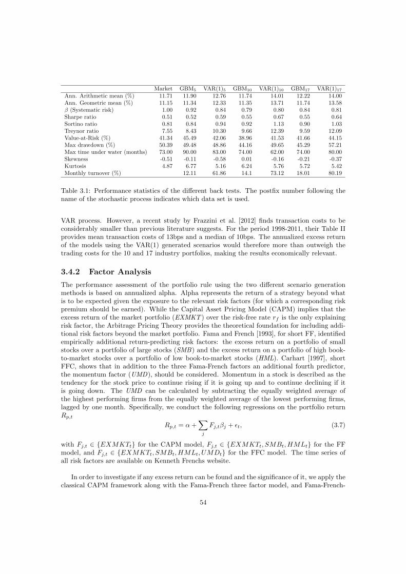
Market GBM5 VAR(1)5 GBM10 VAR(1)10 GBM17 VAR(1)17Ann. Arithmetic mean (%) 11.71 11.90 12.76 11.74 14.01 12.22 14.00Ann. Geometric mean (%) 11.15 11.34 12.33 11.35 13.71 11.74 13.58β (Systematic risk) 1.00 0.92 0.84 0.79 0.80 0.84 0.81Sharpe ratio 0.51 0.52 0.59 0.55 0.67 0.55 0.64Sortino ratio 0.81 0.84 0.94 0.92 1.13 0.90 1.03Treynor ratio 7.55 8.43 10.30 9.66 12.39 9.59 12.09Value-at-Risk (%) 41.34 45.49 42.06 38.96 41.53 41.66 44.15Max drawdown (%) 50.39 49.48 48.86 44.16 49.65 45.29 57.21Max time under water (months) 73.00 90.00 83.00 74.00 62.00 74.00 80.00Skewness -0.51 -0.11 -0.58 0.01 -0.16 -0.21 -0.37Kurtosis 4.87 6.77 5.16 6.24 5.76 5.72 5.42Monthly turnover (%) 12.11 61.86 14.1 73.12 18.01 80.19

Table 3.1: Performance statistics of the different back tests. The postfix number following thename of the stochastic process indicates which data set is used.

VAR process. However, a recent study by Frazzini et al. [2012] finds transaction costs to beconsiderably smaller than previous literature suggests. For the period 1998-2011, their Table IIprovides mean transaction costs of 13bps and a median of 10bps. The annualized excess returnof the models using the VAR(1) generated scenarios would therefore more than outweigh thetrading costs for the 10 and 17 industry portfolios, making the results economically relevant.

3.4.2 Factor Analysis

The performance assessment of the portfolio rule using the two different scenario generationmethods is based on annualized alpha. Alpha represents the return of a strategy beyond whatis to be expected given the exposure to the relevant risk factors (for which a corresponding riskpremium should be earned). While the Capital Asset Pricing Model (CAPM) implies that theexcess return of the market portfolio (EXMKT ) over the risk-free rate rf is the only explainingrisk factor, the Arbitrage Pricing Theory provides the theoretical foundation for including addi-tional risk factors beyond the market portfolio. Fama and French [1993], for short FF, identifiedempirically additional return-predicting risk factors: the excess return on a portfolio of smallstocks over a portfolio of large stocks (SMB) and the excess return on a portfolio of high book-to-market stocks over a portfolio of low book-to-market stocks (HML). Carhart [1997], shortFFC, shows that in addition to the three Fama-French factors an additional fourth predictor,the momentum factor (UMD), should be considered. Momentum in a stock is described as thetendency for the stock price to continue rising if it is going up and to continue declining if itis going down. The UMD can be calculated by subtracting the equally weighted average ofthe highest performing firms from the equally weighted average of the lowest performing firms,lagged by one month. Specifically, we conduct the following regressions on the portfolio returnRp,t

Rp,t = α+∑j

Fj,tβj + εt, (3.7)

with Fj,t ∈ EXMKTt for the CAPM model, Fj,t ∈ EXMKTt, SMBt, HMLt for the FFmodel, and Fj,t ∈ EXMKTt, SMBt, HMLt, UMDt for the FFC model. The time series ofall risk factors are available on Kenneth Frenchs website.

In order to investigate if any excess return can be found and the significance of it, we apply theclassical CAPM framework along with the Fama-French three factor model, and Fama-French-

54

Carhart four factor model. We test the significance of the excess return in terms of p-valuesand analyze if it can be ascribed to value, small cap and/or momentum. The assessment ofthe out-of-sample back tests when using the three different data sets can be found in Table 3.2,which shows that a positive excess return exists when using the VAR process on all data sets.

CAPM FF FFC

α (%) p-value α (%) p-value α (%) p-value

VAR(1)5 2.30 0.02 2.38 0.02 2.23 0.03GBM5 0.80 0.30 1.95 0.01 0.75 0.31

VAR(1)10 3.85 0.00 2.76 0.01 2.98 0.01GBM10 1.64 0.07 1.71 0.06 0.28 0.75

VAR(1)17 3.69 0.00 2.21 0.06 1.91 0.11GBM17 1.71 0.07 1.45 0.11 -0.13 0.88

Table 3.2: Assessment of annualized α

Furthermore, we observe low p-values, indicating that the excess returns are not a coincidence.Contrary, the geometric Brownian motion provides only a negligible excess return which is non-significant for the most part.When reducing the granularity of the industry portfolios from 5 to 10 or 17, we observe thatthe VAR-process leads to distinctively higher excess returns, showing that the model is able touse a more elaborate dependency pattern. Contrary, no improvement is observed for GBM. TheVAR process is therefore considered to be economically helpful in predicting future returns andto outperformn the market by generating risk-adjusted excess returns. Finally, we extend theanalysis to considering the Sharpe ratio of the strategies.

3.4.3 Sharpe Ratio Analysis

To further investigate the excess performance generated from the assumed predictability of re-turns, we analyze the Sharpe ratio of the strategies and the difference between them.The Sharpe ratio is one of the most widely used performance measures of investment strategies.Though, it has been argued that this measure is not appropriate when returns are not normallydistributed, e.g. when returns experience skewness and leptokurtosis, or are autocorrelated. It istherefore relevant to examine the difference between multiple Sharpe ratios in a robust manner.A popular method for evaluating the difference between two strategies is the test of Jobson andKorkie [1981], which has been corrected by Memmel [2003]. Later, Ledoit and Wolf [2008] discussinference methods that are more generally valid. They suggest computing a HAC standard errorfor the difference of the estimated Sharpe ratios by the methods of Andrews [1991] and Andrewsand Monahan [1992]. Furthermore, they propose to construct a two-sided bootstrap confidenceinterval for the difference. In this paper, we chose to follow the approach of Ledoit and Wolf andcompute p-values in order to test for a significant difference between Sharpe ratios using blockbootstrapping,4.

First, we calculate the Sharpe ratio of the different out-of-sample excess returns by dividingthe mean of the excess returns over the risk free rate by the standard deviation. Following this

4Implementations of the three methods are made available by Ledoit and Wolf at http://www.econ.uzh.ch/

en/people/faculty/wolf/publications.html

55

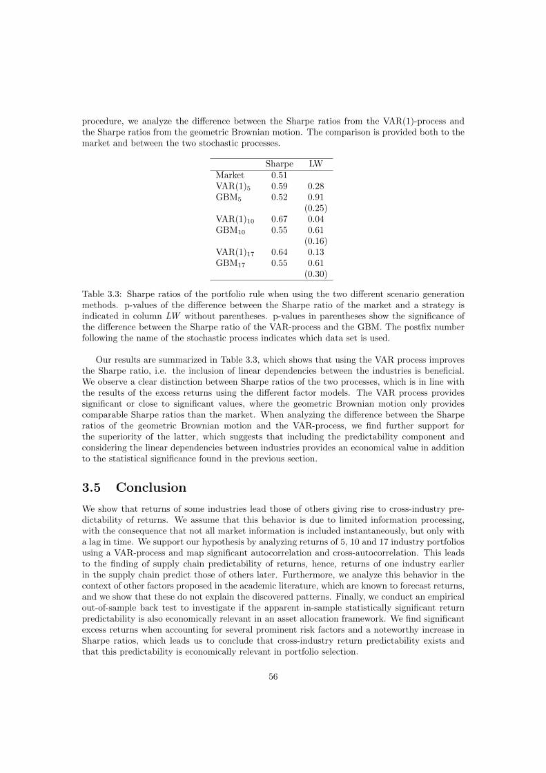
procedure, we analyze the difference between the Sharpe ratios from the VAR(1)-process andthe Sharpe ratios from the geometric Brownian motion. The comparison is provided both to themarket and between the two stochastic processes.

Sharpe LWMarket 0.51VAR(1)5 0.59 0.28GBM5 0.52 0.91

(0.25)VAR(1)10 0.67 0.04GBM10 0.55 0.61

(0.16)VAR(1)17 0.64 0.13GBM17 0.55 0.61

(0.30)

Table 3.3: Sharpe ratios of the portfolio rule when using the two different scenario generationmethods. p-values of the difference between the Sharpe ratio of the market and a strategy isindicated in column LW without parentheses. p-values in parentheses show the significance ofthe difference between the Sharpe ratio of the VAR-process and the GBM. The postfix numberfollowing the name of the stochastic process indicates which data set is used.

Our results are summarized in Table 3.3, which shows that using the VAR process improvesthe Sharpe ratio, i.e. the inclusion of linear dependencies between the industries is beneficial.We observe a clear distinction between Sharpe ratios of the two processes, which is in line withthe results of the excess returns using the different factor models. The VAR process providessignificant or close to significant values, where the geometric Brownian motion only providescomparable Sharpe ratios than the market. When analyzing the difference between the Sharperatios of the geometric Brownian motion and the VAR-process, we find further support forthe superiority of the latter, which suggests that including the predictability component andconsidering the linear dependencies between industries provides an economical value in additionto the statistical significance found in the previous section.

3.5 Conclusion

We show that returns of some industries lead those of others giving rise to cross-industry pre-dictability of returns. We assume that this behavior is due to limited information processing,with the consequence that not all market information is included instantaneously, but only witha lag in time. We support our hypothesis by analyzing returns of 5, 10 and 17 industry portfoliosusing a VAR-process and map significant autocorrelation and cross-autocorrelation. This leadsto the finding of supply chain predictability of returns, hence, returns of one industry earlierin the supply chain predict those of others later. Furthermore, we analyze this behavior in thecontext of other factors proposed in the academic literature, which are known to forecast returns,and we show that these do not explain the discovered patterns. Finally, we conduct an empiricalout-of-sample back test to investigate if the apparent in-sample statistically significant returnpredictability is also economically relevant in an asset allocation framework. We find significantexcess returns when accounting for several prominent risk factors and a noteworthy increase inSharpe ratios, which leads us to conclude that cross-industry return predictability exists andthat this predictability is economically relevant in portfolio selection.

56

Bibliography

Donald WK Andrews. Heteroskedasticity and autocorrelation consistent covariance matrix esti-mation. Econometrica, 59(3):817–858, 1991.

Donald WK Andrews and J Christopher Monahan. An improved heteroskedasticity and auto-correlation consistent covariance matrix estimator. Econometrica, 60(4):953–966, 1992.

Andrew Ang and Geert Bekaert. Stock return predictability: Is it there? Review of FinancialStudies, 20(3):651–707, 2007.

Philippe Artzner, Freddy Delbaen, Jean-Marc Eber, and David Heath. Coherent measures ofrisk. Mathematical Finance, 9(3):203–228, 1999.

Doron Avramov. Stock return predictability and asset pricing models. Review of FinancialStudies, 17(3):699–738, 2004.

Doron Avramov and Russ Wermers. Investing in mutual funds when returns are predictable.Journal of Financial Economics, 81(2):339–377, 2006.

Ray Ball. Anomalies in relationships between securities’ yields and yield-surrogates. Journal ofFinancial Economics, 6(2):103–126, 1978.

Ravi Bansal and Amir Yaron. Risks for the long run: A potential resolution of asset pricingpuzzles. The Journal of Finance, 59(4):1481–1509, 2004.

Geert Bekaert and Robert J Hodrick. Characterizing predictable components in excess returnson equity and foreign exchange markets. The Journal of Finance, 47(2):467–509, 1992.

Thomas Trier Bjerring, Omri Ross, and Alex Weissensteiner. Feature selection for portfoliooptimization. Annals of Operations Research, 2016.

William Breen, Lawrence R Glosten, and Ravi Jagannathan. Economic significance of predictablevariations in stock index returns. The Journal of Finance, 44(5):1177–1189, 1989.

John Y Campbell. Stock returns and the term structure. Journal of Financial Economics, 18(2):373–399, 1987.

John Y Campbell and John H Cochrane. By force of habit: A consumption-based explanationof aggregate stock market behavior. Technical report, National Bureau of Economic Research,1995.

John Y Campbell and Robert J Shiller. Stock prices, earnings, and expected dividends. TheJournal of Finance, 43(3):661–676, 1988.

57

John Y Campbell and Robert J Shiller. The dividend-price ratio and expectations of futuredividends and discount factors. The Review of Financial Studies, 1(3):195–228, 1989.

John Y Campbell and Luis M Viceira. Strategic asset allocation: Portfolio choice for long-terminvestors. Oxford University Press, USA, 2002.

John Y Campbell and Tuomo Vuolteenaho. Inflation illusion and stock prices. Technical report,National Bureau of Economic Research, 2004.

John Y Campbell and Motohiro Yogo. Efficient tests of stock return predictability. Journal ofFinancial Economics, 81(1):27–60, 2006.

John Y Campbell, Yeung Lewis Chan, and Luis M Viceira. A multivariate model of strategicasset allocation. Journal of Financial Economics, 67(1):41–80, 2003.

Mark M Carhart. On persistence in mutual fund performance. The Journal of Finance, 52(1):57–82, 1997.

John H Cochrane. Where is the market going? Uncertain facts and novel theories. Technicalreport, National Bureau of Economic Research, 1998.

John H Cochrane. State-space vs. VAR models for stock returns. Unpublished manuscript, 2008.

Lauren Cohen and Andrea Frazzini. Economic links and predictable returns. The Journal ofFinance, 63(4):1977–2011, 2008.

Edmund A Cornish and Ronald A Fisher. Moments and cumulants in the specification of distri-butions. Revue de l’Institut international de Statistique, pages 307–320, 1938.

David M Cutler, James M Poterba, and Lawrence H Summers. Speculative dynamics. TheReview of Economic Studies, 58(3):529–546, 1991.

Thomas Dangl and Michael Halling. Predictive regressions with time-varying coefficients. Journalof Financial Economics, 106(1):157–181, 2012.

Victor DeMiguel, Lorenzo Garlappi, and Raman Uppal. Optimal versus naive diversification:How inefficient is the 1/N portfolio strategy? Review of Financial Studies, 22(5):1915–1953,2009.

Gerben Driesprong, Ben Jacobsen, and Benjamin Maat. Striking oil: Another puzzle? Journalof Financial Economics, 89(2):307–327, 2008.

Bradley Efron. Nonparametric estimates of standard error: The jackknife, the bootstrap andother methods. Biometrika, 68(3):589–599, 1981.

Eugene F Fama. Stock returns, real activity, inflation, and money. The American EconomicReview, 71(4):545–565, 1981.

Eugene F Fama and Kenneth R French. Dividend yields and expected stock returns. Journal ofFinancial Economics, 22(1):3–25, 1988.

Eugene F Fama and Kenneth R French. Business conditions and expected returns on stocks andbonds. Journal of Financial Economics, 25(1):23–49, 1989.

Eugene F Fama and Kenneth R French. Common risk factors in the returns on stocks and bonds.Journal of Financial Economics, 33(1):3–56, 1993.

58

Eugene F Fama and G William Schwert. Asset returns and inflation. Journal of FinancialEconomics, 5(2):115–146, 1977.

Miguel A Ferreira and Pedro Santa-Clara. Forecasting stock market returns: The sum of theparts is more than the whole. Journal of Financial Economics, 100(3):514–537, 2011.

Wayne E Ferson and Campbell R Harvey. The risk and predictability of international equityreturns. Review of Financial Studies, 6(3):527–566, 1993.

Wayne E Ferson, Campbell R Harvey, et al. The variation of economic risk premiums. Journalof Political Economy, 99(2):385–415, 1991.

Andrea Frazzini, Ronen Israel, and Tobias J Moskowitz. Trading costs of asset pricing anomalies.Fama-Miller Working Paper, 2012.

Alois Geyer, Michael Hanke, and Alex Weissensteiner. No-arbitrage bounds for financial scenar-ios. European Journal of Operational Research, 236(2):657–663, 2014.

Campbell R Harvey. The world price of covariance risk. The Journal of Finance, 46(1):111–157,1991.

Sam James Henkel, J Spencer Martin, and Federico Nardari. Time-varying short-horizon pre-dictability. Journal of Financial Economics, 99(3):560–580, 2011.

Erik Hjalmarsson. Predicting global stock returns. Journal of Financial and Quantitative Anal-ysis, 45(1):49–80, 2010.

Robert J Hodrick. Dividend yields and expected stock returns: Alternative procedures forinference and measurement. Review of Financial studies, 5(3):357–386, 1992.

Harrison Hong and Jeremy C Stein. A unified theory of underreaction, momentum trading, andoverreaction in asset markets. The Journal of Finance, 54(6):2143–2184, 1999.

Harrison Hong, Walter Torous, and Rossen Valkanov. Do industries lead stock markets? Journalof Financial Economics, 83(2):367–396, 2007.

Kjetil Høyland, Michal Kaut, and Stein W Wallace. A heuristic for moment-matching scenariogeneration. Computational Optimization and Applications, 24(2-3):169–185, 2003.

J Dave Jobson and Bob M Korkie. Performance hypothesis testing with the sharpe and treynormeasures. The Journal of Finance, 36(4):889–908, 1981.

Michal Kaut and Stein W Wallace. Evaluation of scenario-generation methods for stochasticprogramming. 2003.

Con Keating, Hyun Song Shin, Charles Goodhart, Jon Danielsson, et al. An academic responseto basel II. Technical report, Financial Markets Group, 2001.

VS Kirilyuk. Maximizing the Omega ratio by two linear programming problems. Cyberneticsand Systems Analysis, 49(5):699–705, 2013.

Mark Kritzman, Sebastien Page, and David Turkington. In defense of optimization: The fallacyof 1/n. Financial Analysts Journal, 66(2):31–39, 2010.

Pavlo Krokhmal, Jonas Palmquist, and Stanislav Uryasev. Portfolio optimization with condi-tional value-at-risk objective and constraints. Journal of Risk, 4:43–68, 2002.

59

Oliver Ledoit and Michael Wolf. Robust performance hypothesis testing with the Sharpe ratio.Journal of Empirical Finance, 15(5):850–859, 2008.

Martin Lettau and Sydney Ludvigson. Consumption, aggregate wealth, and expected stockreturns. The Journal of Finance, 56(3):815–849, 2001.

Jonathan Lewellen. Predicting returns with financial ratios. Journal of Financial Economics, 74(2):209–235, 2004.

John Lintner. Inflation and security returns. The Journal of Finance, 30(2):259–280, 1975.

R Douglas Martin, Svetlozar Zari Rachev, and Frederic Siboulet. Phi-alpha optimal portfoliosand extreme risk management. The Best of Wilmott 1: Incorporating the Quantitative FinanceReview, 1:223, 2003.

Helmut Mausser and Dan Rosen. Beyond var: From measuring risk to managing risk. In Compu-tational Intelligence for Financial Engineering, 1999.(CIFEr) Proceedings of the IEEE/IAFE1999 Conference on, pages 163–178. IEEE, 1999.

Christoph Memmel. Performance hypothesis testing with the Sharpe ratio. Finance Letters, 1(1), 2003.

Lior Menzly and Oguzhan Ozbas. Cross-industry momentum. In AFA 2005 Philadelphia Meet-ings, 2006.

Lior Menzly, Tano Santos, and Pietro Veronesi. Understanding predictability. Journal of PoliticalEconomy, 112(1):1–47, 2004.

Robert C Merton. A simple model of capital market equilibrium with incomplete information.The Journal of Finance, 42(3):483–510, 1987.

Wlodzimierz Ogryczak and Andrzej Ruszczynski. Dual stochastic dominance and quantile riskmeasures. International Transactions in Operational Research, 9(5):661–680, 2002.

L’ubos Pastor and Robert F Stambaugh. Predictive systems: Living with imperfect predictors.The Journal of Finance, 64(4):1583–1628, 2009.

Georg Ch Pflug. Some remarks on the value-at-risk and the conditional value-at-risk. ProbabilisticConstrained Optimization: Methodology and Applications, 49:272, 2000.

Joshua Matthew Pollet. Predicting asset returns with expected oil price changes. Available atSSRN 722201, 2005.

David E Rapach, Jack K Strauss, and Guofu Zhou. Out-of-sample equity premium prediction:Combination forecasts and links to the real economy. Review of Financial Studies, 23(2):821–862, 2010.

R Tyrrell Rockafellar and Stanislav Uryasev. Conditional value-at-risk for general loss distribu-tions. Journal of Banking & Finance, 26(7):1443–1471, 2002.

Michael S Rozeff. Dividend yields are equity risk premiums. The Journal of Portfolio Manage-ment, 11(1):68–75, 1984.

Robert C Shiller. Irrational exuberance. Philosophy & Public Policy Quarterly, 20(1):18–23,2000.

60

Robert J Shiller, Stanley Fischer, and Benjamin M Friedman. Stock prices and social dynamics.Brookings Papers on Economic Activity, 1984(2):457–510, 1984.

Christopher A Sims. Rational inattention: A research agenda. Technical report, Discussionpaper Series 1/Volkswirtschaftliches Forschungszentrum der Deutschen Bundesbank, 2005.

Bruno Solnik. The performance of international asset allocation strategies using conditioninginformation. Journal of Empirical Finance, 1(1):33–55, 1993.

Lars Qvigstad Sørensen. Oil price shocks and stock return predictability. In EFA 2009 BergenMeetings Paper, 2009.

Stoyan V Stoyanov, Svetlozar T Rachev, and Frank J Fabozzi. Optimal financial portfolios.Applied Mathematical Finance, 14(5):401–436, 2007.

Ivo Welch and Amit Goyal. A comprehensive look at the empirical performance of equity premiumprediction. Review of Financial Studies, 21(4):1455–1508, 2008.

61

Chapter 4

Portfolio Optimization ofCommodity Futures withSeasonal Components and HigherMomentsThomas Trier Bjerring · Kourosh Marjani Rasmussen · Alex Weissensteiner

Status: Submitted, Journal of Asset Management

Abstract: We investigate the diversification benefits of combining commodi-ties with a traditional equity portfolio, while considering higher order sta-tistical moments and seasonality. The literature suggests that the in-samplediversification benefits of commodities in portfolio optimization are not pre-served out-of-sample. We provide an extensive in-sample and out-of-sampleanalysis with ten commodities and a stock index using the classical tangencymean-variance model and the maximum Omega ratio model. We show thatseasonality in commodity returns should be considered, and leads to signifi-cant excess return and increase in Sharpe ratio.

Keywords: Commodity Futures, Sieve Bootstrapping, Omega Ratio, Portfo-lio Optimization, Stochastic Programming

4.1 Introduction

In recent years, the consideration of alternative investments in portfolio selection has receivedincreasing attention, which among others has lead to an escalating financialization of the com-modity markets. Several studies find beneficial properties when adding commodity futures toan already diversified equity or equity/bond portfolio. The natural justification of includingcommodity futures in an investment portfolio is the natural hedge they provide against infla-tion, see Bodie [1983]. An inflationary environment is characterized by a sustained increase incommodity prices, meaning that long positions in future contracts increase in value during suchperiods, where stocks and bonds, by contrast, generally display poor performance [see Bodie,1983, Greer, 1978, Halpern and Warsager, 1998, Becker and Finnerty, 2000]. Furthermore, re-

63

turns of commodity investments show low or even negative correlation with the returns of assetsthat belong to traditional asset classes such as equity or debt holdings. This can be ascribed tothe underlying factors that drive commodity prices (e.g., weather and geopolitical events, supplyand demand in the physical production, or event risk). These factors are distinctly different fromwhat determines the value of stocks and bonds [see Geman, 2005, for a dicussion]. In fact, anumber of empirical studies confirm low correlation over certain periods of time [see Bodie andRosansky, 1980, Erb and Harvey, 2006, Gorton and Rouwenhorst, 2006, Geman and Kharoubi,2008, Buyuksahin et al., 2010, Chong and Miffre, 2010]. Consequently, diversification benefits,i.e. reduction of risk for any given level of expected return, emerge.

In this paper we focus on the role of commodities in tactical asset allocation decisions, whencombined with a broad equity index. A strand of literature investigates whether incorporatingcommodities in the asset menu improves the risk-return profile of investors’ portfolios. Bodieand Rosansky [1980], Fortenbery and Hauser [1990] and Conover et al. [2010] find that investorscan improve their risk return payoff by switching from a pure stock portfolio to a portfolio withstocks and commodities over the periods 1950-1976, 1976-1985, and 1970-2007, respectively.Georgiev [2001] performs a similar analysis over the period 1995-2005 and finds an increase inthe Sharpe ratio. In addition, a number of studies investigate the role of commodities underthe Markowitz mean-variance asset allocation setting and reach similar conclusions. Ankrimand Hensel [1993] study the diversification benefits of investing in commodities over the period1972-1990, and conclude that expanding the investable universe with commodities improves therisk-return trade-off of optimal portfolios for any given risk tolerance coefficient. Satyanarayanand Varangis [1996] and Abanomey and Mathur [1999] examine whether the efficient frontierchanges when commodity futures are incorporated into international assets universes over theperiods 1970-1992 and 1970-1995, respectively. They find that the inclusion of commoditiesshifts the efficient frontier upwards. Anson [1999] addresses the same question from anotherperspective. He forms optimal portfolios by maximizing a quadratic expected utility functionfor a range of risk aversion coefficients over the period 1974-1997. He concludes that addingcommodities to a portfolio of stocks and bonds increases the Sharpe ratio of optimal portfolios.Jensen et al. [2000] also find that including commodities in a traditional asset universe improvesthe risk-return profile of the efficient portfolios over the period 1973-1997. Idzorek et al. [2007]performs a similar empirical analysis over the period 1970-2005 with comparable conclusions.Hence, the above mentioned literature has provided unanimous evidence that an investor couldbenefit from including commodities in a diversified portfolio. However, this conclusion is basedon an in-sample mean-variance comparison of the efficient frontier with and without inclusionof commodities. Daskalaki and Skiadopoulos [2011] revisit the in-sample setting by employingmean-variance and non-mean-variance spanning tests and confirm the diversification benefits ofincluding commodities in the asset menu. They then form optimal portfolios by taking intoaccount the higher order moments of the portfolio return distribution and asses their out-of-sample performance. They find that the adherent increase in Sharpe ratio is not preserved fromthe in-sample setting, and hereby challenge the alleged diversification benefits of commodities.A criticism that is often raised against the Sharpe ratio and the mean-variance framework is thatit is only appropriate when the portfolio returns are elliptically distributed. Hence, only the firstand second order statistical moments of the portfolio returns are taken into account, and higherorder moments are neglected, i.e. if asset returns exhibit fat tails, then the Sharpe Ratio yieldscounter-intuitive performance evaluations. Therefore, maximization of the portfolio Sharpe ratiois not appropriate when returns do not follow a normal or elliptical distribution. There existsample empirical evidence that returns of traditional financial products are rarely normally dis-tributed, e.g. Peiro [1999] illustrates this for stock indexes, while Gorton and Rouwenhorst [2006]

64

and Kat and Oomen [2007] reach the same conclusions for commodity futures. Hence, the usualadapted approach based on the first two statistical moments may not be suited to investigatethe in-sample and out-of-sample performance of including commodities in the asset menu.

This paper adds to the existing literature on the role of commodities in portfolio optimiza-tion by analyzing the empirical distribution of the Sharpe ratio of various commodities alongwith the impact of seasonality in commodity returns on the allocation of assets in an in-sampleand out-of-sample mean-variance setting. Furthermore, we propose to use the Omega ratio inportfolio optimization in order to account for higher order statistical moments. We conduct ouranalysis using monthly data for 10 highly traded continuous future contracts on commoditiestogether with a broad equity portfolio over the period 1975.01 - 2014.12.

The rest of the paper is structured as follows. Section 2 outlines the data used throughoutthe paper. Section 3 conducts an in-sample analysis of the empirical distribution of the Sharperatio of different continuous commodity future contracts. Section 4 describes the models. Sec-tion 5 computes the efficient frontier when considering the variance and lower partial momentas risk measures. Section 6 conducts an out-of-sample analysis of the performance of the com-modity/equity portfolios using the different described models. Finally, Section 7 summarizes theresults.

4.2 Data

We use monthly returns of ten active traded commodity futures and of the U.S. equity market.The commodity futures are collected from Bloomberg, while we use the value-weighted returnsof all NYSE, AMEX, and NASDAQ firms to proxy the U.S. equity market, which are providedas market returns in French’s data library.1 We use ten continuous future contracts on individualcommodities from distinctively different categories: Gold, Silver, Platinum, Copper, Soybean,Lumber, Coffee, Feeder Cattle, Lean Hogs, and Live Cattle. The underlying dynamics of com-modity returns differ from those of stocks, as prices are mainly driven by demand and supplyshocks, and consumer behavior [see Gorton et al., 2013].

The properties of commodity derivatives and their correlation to the stock and bond marketshave been explored by Gorton and Rouwenhorst [2006], who find that the long term correlationof an equally weighted index of commodity futures to the stock- and bond market is negative.Furthermore, they also report that the short horizon correlation is nearly zero, making com-modity futures interesting components of a well-diversified portfolio. We find that our chosencommodities all exhibit low correlation to the stock market, see Table 4.1.

The assets with the lowest correlation to the equity market is Gold followed by Coffee andCattle. The low correlation to the equity markets is not the only attractive property of commodi-ties. Empirical evidence shows that under certain market conditions commodities can providereturns similar to equity, e.g. during periods with high inflation or around crises in traditionalfinancial markets [see Skiadopoulos, 2012, Bhardwaj et al., 2015]. We summarize the statisticalmoments of the individual considered assets in Table 4.2.

Out of all considered assets, equities have the highest average return and the lowest standarddeviation. Furthermore, while equities are normally left skewed, all the considered commoditiesare right skewed, illustrating one of the differences between equity and commodities.

1French’s Data Library: http://mba.tuck.dartmouth.edu/pages/faculty/ken.french/data_library.html

65

Gold Silver Platinum Copper Soybean Lumber Coffee Feeder Lean LiveCattle Hogs Cattle

Silver 0.74Platinum 0.66 0.65Copper 0.35 0.38 0.42Soybean 0.13 0.17 0.15 0.25Lumber 0.05 0.09 0.13 0.12 0.08Coffee 0.06 0.11 0.13 0.12 0.21 0.11FeederCattle -0.04 0.03 0.08 0.09 0.00 0.11 -0.07LeanHogs 0.05 0.10 0.07 0.03 0.08 0.09 -0.04 0.27LiveCattle 0.03 0.06 0.14 0.08 0.04 0.07 -0.02 0.69 0.26Equity 0.04 0.15 0.16 0.30 0.11 0.21 0.04 0.09 0.05 0.05

Table 4.1: Correlation matrix

Mean St.dev Skewness Excess kurtosisGold 0.56 5.71 0.66 6.91Silver 0.72 9.42 0.53 8.07Platinum 0.70 7.52 0.27 6.85Copper 0.65 7.62 0.08 5.63Soybean 0.31 8.13 0.38 5.09Lumber 0.68 9.60 0.47 3.95Coffee 0.80 11.17 1.12 6.55Feeder Cattle 0.53 4.79 0.10 4.80Lean Hogs 0.49 9.20 0.19 4.34Live Cattle 0.44 5.27 0.02 3.72Equity 1.09 4.49 -0.65 5.22

Table 4.2: Summary statistics showing arithmetic mean, standard deviation, skewness and excesskurtosis of monthly returns

4.3 Distribution of the Sharpe Ratio

Investment strategies and financial assets are often assessed by their Sharpe ratio, despite theparticular measure having several clear drawbacks, such as the assumption of returns being i.i.dand normal distributed [see Ledoit and Wolf, 2008]. Though, as this measure is the adoptedindustry standard, we analyze our investment universe in this context to further uncover theusefulness of commodities. The true parameters of financial assets are not observable, and theSharpe ratios therefore have to be estimated from historical return data. In order to comparedifferent Sharpe ratios when returns are not normal distributed, we have to rely on statisticalinference, such as hypothesis tests or confidence intervals. Stocks and bonds typically experienceonly minor serial correlation usually expressed in form of volatility clustering. Contrary, manycommodities show strong intra-annual seasonality, which will have a direct impact on the Sharperatio. In this section, we evaluate the autocorrelation of our considered commodities and theequity portfolio, and bootstrap Sharpe ratio probability distributions.

4.3.1 Seasonal Components

Seasonality is known to be one of the empirical characteristics that make commodities strik-ingly different from stocks, bonds, and other conventional financial products [for a discussion

66

see Routledge et al., 2000]. Rational behavior of market participants alone cannot fully explainthe presence of seasonality in the stock and bond markets, while the existence in the commoditymarkets is potentially explainable by the cyclic nature of production. As agricultural commodi-ties must follow their own crop cycle which repeats the same seasonal patterns year after year,observed commodity prices exhibit nonstationarities along the same seasonal lines. Crop cycle-related seasonalities in agricultural commodities are documented by Roll [1984], Anderson [1985],Milonas and Vora [1985], Kenyon et al. [1987], and Fama and French [1987]. Seasonality is alsofound in the energy sector among fossil fuels, natural gas futures [see Brown and Yucel, 2008],and refined products such as gasoline, heating oil and fuel oil futures [see Adrangi et al., 2001].

The seasonality for each commodity may be unique due to different harvesting seasons andavailability. Thus, the predictable components for each asset have to be considered individually.We uncover the seasonal component for each asset in our investment universe by considering theoptimal number of lags according to Akaike’s information criterion (AIC) when fitting an ARprocess to the individual time series of monthly returns.

Gold Silver Platinum Copper Soybean Lumber Coffee Feeder Lean Live EquityCattle Hogs Cattle

Lags 5 0 0 0 11 12 7 22 24 23 1

Table 4.3: Optimal number of lags according to AIC

Table 4.3 shows that the agricultural commodities Soybean, Lumber, and Coffee all have lagsup to 12 months, which coincide with the commodities expected production cycle. Cattle andHogs show substantial predictability in terms of lags being significant on up to 24 months, or twoyears. The Metal commodities show no seasonality, expect for gold. The seasonality of gold isgenerally assumed to be demand driven and closely linked to holiday shopping and the weddingseason of India and the U.S., which occur end of year and late spring, respectively [see Baur, 2013].

We are interested in the Sharpe ratio of the different considered assets in our investmentuniverse. As the illustrated seasonal behavior will have a huge impact on the performancemeasure at different points in time, we resort to block bootstrap probability distributions for theSharpe ratio, instead of relying on individual statistics.

4.3.2 Sharpe ratio

The Sharpe ratio is defined as the excess return over the risk free rate of a considered asset orportfolio divided by the standard deviation. In order to create a more refined picture of thebenefit of incorporating commodities in a portfolio and the impact on the corresponding Sharperatio, we bootstrap individual distributions of the performance measure for each of the consideredassets. Given that regular bootstrapping requires i.i.d samples, which does not comply with ourdata due to the presence of seasonality, we resort to block bootstrapping. Here, blocks of data aresampled from the data set instead of single data points, hence, preserving the autocorrelation ofthe data. We use circular block bootstrapping to generate 1000 paths of three years of monthlydata. Several criteria have been proposed for selecting the block size, [see Politis and Romano,1994, Politis and White, 2004, Patton et al., 2009, Hall et al., 1995], though in this case, theblock size of the considered asset is fixed to the optimal number of lags plus one in order tocontrol for the seasonal patterns. In the case of no predictive power, i.e. when an asset followsa geometric Brownian motion, the optimal number of lags is zero. As a consequence, the block

67

size is one, and the method coincides with the regular bootstrap approach. After constructinga sample path of 36 months for a given asset, the Sharpe ratio is computed with respect to therisk free rate for the given blocks. The risk free rate is taken as the one-month Treasury bill rate.We repeat the block bootstrapping procedure for each individual asset and compute 0.05, 0.25,0.75, and 0.95 quantiles along with the Sharpe ratio over the complete data period.

Figure 4.1: Block bootstrapped distributions of Sharpe ratios. The light gray line correspondsto 0.05 and 0.95 quantiles, while the dark gray line covers the distance between the 0.25 and 0.75quantiles. The bullets represents the average Sharpe ratio of the given asset.

Figure 4.1 shows that the stock market has a distinctively higher average Sharpe ratio thanthe individual commodities. Furthermore, we observe that most commodities have Sharpe ratioscentered around zero or even negative. Hence, naively incorporating commodities in long-termbuy-and-hold strategies will not improve the performance. Though, the quantiles indicate thattemporary market situations exist, where commodities can provide a valuable alternative to thestock market. The broad stock market does in rare cases experience near-zero or negative Sharperatios. Given the correlation structure, it is natural to assume that in those situations commodi-ties would play an important role in optimizing the return-risk relationship of a portfolio. Toexamine this further, we conduct a similar bootstrap analysis of the correlation coefficient ofa given commodity to the equity market. We bootstrap three year sample paths of monthlyreturns for a given commodity and the equity market using the block size of the commodity, andcompute the correlation coefficient over the constructed period.

Figure 4.2 shows that the correlation of most of the considered commodities extend into thenegative region, making them a valid hedging instrument under certain market conditions. Addi-tionally, we observe that the 0.95-quantile of the correlation coefficient of almost all commoditieswith the stock portfolio is low, supporting the inclusion of commodities in a stock portfolio. Asa comparison, the average correlation of the Fama-French 30 industry portfolios is equal to 0.59over the same period.

4.4 Models

The benefits of including commodities has typically been analyzed in the mean-variance setting.A portfolio is then constructed to either minimize the portfolio variance or maximize the Sharperatio. In order not to confine ourself to Gaussian or elliptical distributions, we consider stochasticprogramming to maximize the Omega ratio. In this section, we first highlight a semi-parametric

68

Figure 4.2: Block bootstrapped distributions of the correlation coefficient of the individual com-modities to the market. The light gray line corresponds to 0.05 and 0.95 quantiles, while thedark gray line covers the distance between the 0.25 and 0.75 quantiles. The bullets representsthe average correlation of the given asset.

scenario generation method to be used in a stochastic programming framework, which incorpo-rates the potential seasonal behavior of the considered commodities. We then provide the modelformulations of the classical tangency mean-variance model and the Omega ratio model.

4.4.1 Sieve Bootstrapping

Stochastic programming requires a discrete approximation of the underlying stochastic processat hand. Given the event history up to a particular time, the uncertainty in the next periodis characterized by finitely many possible realizations of a random variable. Usually, scenariosare created by either taking historic realizations of past returns as possible future outcomes orgenerated by sophisticated models [for an overview, see Kaut and Wallace, 2007].

The application of stochastic programming to commodities requires a discrete representationof the uncertainty which incorporates the distinctive seasonal patterns that we observe for most ofthe commodities. We propose the application of sieve bootstrapping, which is a semi-parametricapproach to model time series data which experience autocorrelation [see Geman and Hwang,1982, Buhlmann et al., 1997]. Regular bootstrapping requires i.i.d. samples, and is thereforeusually inadequate for modeling time series data. Contrary, the sieve bootstrap procedure fitsan autoregressive process with order p to the original data and generates bootstrap samples byresampling the residuals uniformly. As the residuals of the autoregressive model are i.i.d., it isreasonable to resample those randomly - similar to the original bootstrap approach. Comparableto the choice of the block size for block bootstrapping, selecting the lag order of the autogressivemodel is crucial to ensure i.i.d. residuals. Therefore, we choose to rely on AIC to select the orderp. The autoregressive model fitted to the data is of the form

Yt = aYt−1 + ...+ kYt−p + k + εt,

where Y is a random variable, a to k are fitted parameters, p is the maximum number oflags according to the AIC criterion, k is constant and ε are the residuals. The consideredcommodities experience noticeable different seasonality patterns and univariate AR(p) models aretherefore fitted individually to each asset. Following the parameter estimation, we sample from

69

the multivariate residual distribution to construct a set of scenarios preserving the correlationstructure between the considered assets along with higher statistical moments.

Mean-Variance Tangency Portfolio

Portfolio selection in a mean-variance framework is based on the assumption, that asset returnsare normally distributed. We consider the mean-variance model where the investor is faced withthe decision on how to optimally allocate funds to N risky assets. This model maximizes theSharpe ratio of the investor’s portfolio [see Sharpe, 1966]. However, naively using the Sharperatio as objective function gives rise to a non-linear problem formulation, and cannot be solvedanalytically when including constraints. The non-linear problem can be formulated as

max µ>x

x>Σxs.t.

1x = 1x ≥ 0,

where x is the vector of portfolio weights, and µ and Σ denotes the expected return and thevariance-covariance matrix, respectively. The optimization of the nonlinear performance ratiohas typically been addressed by introducing a bi-objective equivalent along with a risk aversionparameter. Hence, the maximum Sharpe ratio portfolio could be obtained by solving a seriesof quadratic programming problems with the objective function, max µ>x − λx>Σx, for recur-sively increasing values of λ. Stoyanov et al. [2007] show that the model can be formulated as afractional-quadratic programming problem, hereby reducing the number of quadratic problemsto be solved to one. They introduce an auxiliary scaling variable z to enable the transformationof the nonlinear programming formulation to a quadratic problem that maximizes the Sharperatio. The model can then be formulates as

min x>Σxs.t.

µjxj − zrf ≥ 1n∑j=1

xj = z,

xj ≥ 0,

Finally, the optimal computed solution x∗ should be normalized by z to be rescaled to the originaldecision space.

Omega-Ratio

Several alternatives to the optimization of the Sharpe ratio have been proposed. Most prominentis Sortino and Price [1994], who replace the standard deviation with the downside deviation.Recently, Keating and Shadwick [2002] introduce the Omega ratio which incorporates highermoment information of a distribution of returns, and captures both the downside and upsidepotential of a portfolio. The rationale behind the formulation of the Omega ratio is that, givena predetermined threshold τ , portfolio returns over the target τ are considered as gains, whereasreturns below the threshold are treated as losses. The Omega ratio can be defined as the ratiobetween the expected value of the gains and the expected value of the losses. The threshold τis selected as a predefined benchmark such as the market return or the risk-free rate. In other

70

words, the Omega ratio considers the first order lower partial moment as a risk measure. Lowerpartial moments have already been considered as risk measures by Nawrocki [1999] and Ogryczakand Ruszczynski [1999]. Unlike the variance, the measure can cope with skewed returns and istherefore more suitable for handling non-normally distributed returns.

The original formulation of the Omega ratio was computational intractable, and was, as aconsequence, mostly used for evaluating investment strategies ex post [see Bertrand and Prigent,2011]. The ratio is defined in terms of a cumulative distribution F of a portfolio, where

Ω(τ) =

∫∞τ

(1− F (x)) dx∫ τ−∞ F (x)dx

.

The Omega ratio is visualized in Figure 4.3, and quantifies the area under the cumulative dis-tribution left of the target value τ , and the area above it to the right. Mausser et al. [2013]

τ

0

0.5

1

−3 0 3

Figure 4.3: The cumulative probability distribution, where τ and the dashed line illustrates thethreshold value.

demonstrate how a simple transformation of the problem variables leads to a LP solvable modelfor maximizing the Omega ratio. The only requirement is that the expected return of the optimalportfolio is larger than that of the benchmark τ . More precisely, the problem is reformulatedas a linear-fractional programming problem, where the portfolio downside deviation from thethreshold is modeled using a continuous variable. Kapsos et al. [2014b] show how the Omegaratio maximization problem can be reformulated as a quasi-concave optimization problem, andthus be solvable in polynomial time. Following this approach, Kapsos et al. [2014a] introduce aworst-case variant of the model maximizing the Omega ratio and investigate its properties underthree types of uncertainty for the probability distribution of the returns. Finally, Guastarobaet al. [2016] use the maximization of the Omega ratio for index tracking, and extend the frac-tional programming model formulation to consider a distribution for the threshold τ instead ofa single parametric value.

The downside function of the Omega ratio is usually expressed in terms of either the semi-standard deviation or the first lower partial moment. We will use the later definition in thispaper as it can be expressed with a linear formulation contrary to the first one, which requiresa quadratic term. The first lower partial moment can be defined as

71

δτ = E(Rx − τ)− = Emaxτ −Rx, 0.

where δτ is LP computable for returns represented by discrete representations as follows, assum-ing pt probability for each scenario (realization)

δτ (Rx) = min

S∑s=1

dsps

∣∣∣∣∣ ds ≥ τ −n∑j=1

rj,sxj , ds ≥ 0

.

We follow the fractional linear programming approach suggested by Mausser et al. [2013] underthe assumption that µ>x > τ , and we adopt the suggestion of Guastaroba et al. [2016] by in-troducing a big M constraint on the risk function. Hence, we ensure that δτ cannot attain thevalue zero hereby making the return/risk fraction infinite. We end up with the following modelfor the maximization of the Omega ratio:

max

n∑j=1

µjxj − τz

s.t.n∑j=1

xj = z

z ≤ Mn∑j=1

rj,sxj = ys

S∑s=1

dsps = 1

ds ≥ τz − ysds ≥ 0 xj ≥ 0,

where z is an auxiliary scaling variable. The optimal portfolio weights w∗ are found as thenormalized solution according to z, w∗j = xj/z.

4.5 The Efficient Frontier

In this section, we examine the in-sample diversification benefits of commodity futures whenapplying the optimal mean-variance portfolio and the maximization of the Omega ratio andconsidering seasonality patterns. We compare the efficient frontier when the two portfolio rulesrely only on sample parameters estimated directly from historical data to those when shievebootstrapping is used. We illustrate the difference using the first 10 years of monthly returnsspanning over the period 1975.01-1985.01 and we examine the efficient frontiers. The data windowis intensionally chosen to be large to reduce the risk of parameter uncertainty. Furthermore, welimit the maximum number of lags to 12 to avoid overfitting the data.

Figure 4.4 shows that including seasonality in the mean and variance estimation extends theefficient frontier into a region which was not covered by a setting without predictability. It canbe observed that a small risk reduction can be found when including seasonality, along with asignificant increase in expected return. The maximum Omega ratio portfolios do in both casesrepresent more risk adverse strategies than their corresponding mean-variance counterparts whenrisk is evaluated in terms of standard deviation. This is found to be rooted in the consideration

72

Figure 4.4: Efficient mean-variance frontier for the period 1975.01-1985.01. The solid and dashedlines represent the efficient frontiers when including or excluding seasonality, respectively. Thetangency portfolio for each frontier is illustrated with a bullet. The gray bullets represent thecorresponding maximum Omega ratio portfolios. The risk free rate is fixed to zero.

of higher statistical moments, which leads to a more prudent asset allocation.

In order to analyze whether the benefits of considering predictability have economic relevance,it is necessary to consider the portfolio rules in an out-of-sample environment. In such an out-of-sample setting, most papers find less support for the inclusion of commodities in an alreadydiversified equity or equity/bond portfolio.

4.6 Empirical Application

The classical mean-variance model using the sample mean and covariance matrix as inputs hasbeen shown to perform poorly out-of-sample, and that the apparent in-sample diversificationbenefits of including commodities in a portfolio are not preserved. In order to test our hypoth-esis that neglecting seasonality when using commodities patterns are one of the reasons for thispoor performance, we test the tangency mean-variance model and maximum Omega ratio model,when parameters are estimated from scenarios generated using the shieve bootstrap procedureand when the sample parameters are estimated directly from data.

The out-of-sample analysis is based on the data set earlier presented and is conducted suchthat we only use data up to a certain point in time to perform a portfolio decision upon. Theoutcome of a decision is computed using the actual end of month returns. We rebalance eachportfolio rule on a monthly frequency and use 10 years of monthly data for parameter estimation.After computing the realized returns of a given month, we move one month ahead in our data setand repeat the procedure. In order to consider time varying investment opportunities, we adopt

73

a rolling parameter window approach, meaning that every time we move one month ahead in ourback test, we discard the oldest data point and include the newest available one. Furthermore,we limit the shieve bootstrap approach to a maximum of 12 lags to avoid overfitting the data,and to extend the back test period (as some commodities experience up to 24 significant timelags). The lag-structure is re-estimated for each time interval, and we exclude short-sales.

4.6.1 Performance Measures

We test the quality of our out-of-sample results using different performance measures on eachof the four conducted back tests, i.e. maximum Omega ratio using historical data or shievebootstrapping, and the tangency mean-variance model using sample parameters from historicaldata or shieve bootstrapping.One of the measures we use to asses the performance is annualized excess return over what wouldbe expected given the exposure to the relevant risk factors (for which a corresponding risk pre-mium should be earned). While the Capital Asset Pricing Model (CAPM) implies that the excessreturn of the market portfolio (EXMKT ) over the risk-free rate r is the only explaining riskfactor, the Arbitrage Pricing Theory provides the theoretical foundation for including arbitrary(additional) risk factors beyond the market portfolio. Fama and French [1993], for short FF,identified empirically additional return-predicting risk factors: the excess return on a portfolio ofsmall stocks over a portfolio of large stocks (SMB) and the excess return on a portfolio of highbook-to-market stocks over a portfolio of low book-to-market stocks (HML). Carhart [1997]shows that a fourth predictor should be considered in addition to the three Fama-French factors,the momentum factor (UMD), short FFC. Momentum in a stock is described as the tendencyfor the stock price to continue rising if it is going up and to continue declining if it is goingdown. The UMD can be calculated by subtracting the equally weighted average of the highestperforming firms from the equally weighted average of the lowest performing firms, lagged byone month. Specifically, we conduct the following regressions

Rp,t − rt = α+∑j

Fj,tβj + εt,

with Fj,t ∈ EXMKTt for the CAPM model, Fj,t ∈ EXMKTt, SMBt, HMLt for the FFmodel, and Fj,t ∈ EXMKTt, SMBt, HMLt, UMDt for the FFC model. The time series ofall risk factors are available on Kenneth French’s website.

Several performance ratios have be developed over the years, but we will in our analysis limitourself to four measures i.e. the Sharpe ratio, the Sortino ratio, the Omega ratio, and the Treynorratio. The most prominent measure is the Sharpe ratio which is defined as the excess return overthe standard deviation. Sortino and Price [1994] suggests using the Sortino ratio instead, whichreplaces the standard deviation of the Sharpe ratio with the downside deviation. The Treynorratio divides the average annualized return with the beta from the CAPM analysis, herebyquantifying the relationship between return and systematic risk. We extend our analysis toexamining the Cornish-Fisher expansion of Value-at-Risk [see Cornish and Fisher, 1938], whichconsiders skewness and excess kurtosis contrary to the traditional formulation. Furthermore,we investigate the maximum drawdown of a portfolio rule. A drawdown is measured on thecumulative returns of a portfolio rule from the time a retrenchment begins to when a new highis reached. Additionally, the maximum Time under Water is computed, which measures themaximum time spent to recovery from a drawdown.

74

4.6.2 Out-of-Sample Analysis

We start the out-of-sample back test on January 1985 to allow for a sufficient parameter estima-tion window of 10 years of monthly return data. The back test is conducted until December 2014.The length of the back test is limited to this period due to data availability from Bloomberg.This results in a total of 360 trading months. We have summarized our key findings of thefour out-of-sample backtests using the defined investment menu of one equity portfolio and 10commodities in the Table 4.4. In the CAPM analysis the market is assumed to correspond toour equity portfolio. Furthermore, we use the one-month treasury bill rate as risk free rate, rf .

Market Omegaboot Omegahist.data TPboot TPhist.dataAlphaCAPM (%) 8.07 -1.76 6.94 -1.97(p.value) (0.00) (0.27) (0.01) (0.22)AlphaFF (%) 9.46 1.24 8.38 1.07(p.value) (0.00) (0.42) (0.00) (0.49)AlphaFFC (%) 9.47 1.14 8.44 1.03(p.value) (0.00) (0.46) (0.00) (0.51)Beta 1.00 0.38 0.58 0.40 0.59Sharpe ratio 0.30 0.82 0.42 0.78 0.40Sortino ratio 0.43 1.43 0.64 1.29 0.60Omega ratio 1.49 2.25 1.72 2.19 1.70Treynor ratio 4.71 34.83 8.89 29.35 8.6099% VaR (Cornish-Fisher) -49.18 -41.93 -38.01 -47.55 -39.99Max Drawdown (%) 54.36 36.08 35.68 38.14 37.22Max Time under Water (months) 73 23 67 29 72Skewness -0.92 -0.37 -0.76 -0.73 -0.87Excess Kurtosis 5.72 5.37 5.68 6.53 6.08Positive months (%) 62.50 63.61 62.78 64.72 62.78Average monthly turnover (%) 64.39 5.7 60.80 4.71

Table 4.4: Summary statistics for the out-of-sample back test of the equity market and the fourportfolio strategies, where Omega and TP refer to the maximum Omega ratio portfolio and thetangency mean-variance portfolio, respectively. The prefix following a portfolio rule indicatesthe parameter estimation process.

Table 4.4 shows that the consideration of seasonality results in a significant increase in excessreturn compared to the pure equity portfolio, while the traditional sample approach of parame-ters results in a small decline in excess return. Additionally, we observe that the positive alpha isnot due to the exploitation of momentum or other well-known factors. Furthermore, we find clearoverall reduction in market risk (expressed in beta) by including commodities in the portfolio.Additionally, all four performance ratios support the use of commodities for this particular dataset, i.e. including seasonality in the scenario generation improves the ratios, which are morethan twice than that of the market, showing that there is direct value in combining commoditieswith an equity portfolio. Cornish-Fisher VaR99% of the different models is lower than that of themarket. This reduction in risk is further supported by the size of the maximum drawdown ex-perienced through the out-of-sample back test, which in all cases takes place during the crash ofthe financial markets in 2007. The strategies using the sieve bootstrapping procedure both havelarge reductions in Time under Water compared to the corresponding strategies using historicalsample estimates. This evidence suggests that a better use of commodities in the portfolio set-

75

ting is obtainable from the improved parameter estimation in environments which are typicallycharacterized by high inflation.Overall, our findings support the poor out-of-sample performance observed in the literaturewhen using parameters estimated directly from historical data. Though, the inclusion of theseasonal component in the parameter estimation shows that excess returns over the market canbe increased significantly while reducing risk. Furthermore, the maximum Omega ratio modeloutperforms the classical tangency mean-variance model, hinting that the incorporation of higherorder moments in the portfolio selection process holds direct economic value.The two models relying on shieve bootstrapped scenarios both experience higher turnovers com-pared to the models using sample estimates. The low turnover observed for Omegahist.data andTPhist.data comes from two large portfolio positions in Gold and Equity, which are held nearlyconstant over time. These positions corresponds on average to 64% of the total portfolio overtime. A recent study by Frazzini et al. [2012] finds transactions costs to be much smaller thanprevious literature suggests. For the period 1998-2011, their Table II provides mean transactionscosts of 13bps and a median of 10bps. Therefore, the annualized excess return of the modelsbased on shieve bootstrapping would more than outweigh such trading costs.

Overall, our considered commodity asset universe can be divided into two groups. One con-sisting of commodities that can be categorized as scarce or non-producible (metals), and anotherwhere availability are strongly connected to demand. The latter group includes commoditiessuch as Soybean and Live Cattle where a foreseeable future demand can be met with an increasein production. The first group is often considered as a safe haven in case of financial turmoil.Especially gold is a notorious choice due to its low correlation with the equity markets. It istherefore of interest to consider the out-of-sample back test when the four metals are omittedfrom the investment universe.

Table 4.5 shows the out-of-sample backtest when Gold, Silver, Platinium, and Copper areremoved from the asset menu. Our results are qualitatively similar when using shieve boot-strapping. Considering only the strategies using sample estimates from historic returns, we findthat the diversification benefits are preserved in terms of lower beta, higher performance ratiosthan the market, and a lower Value-at-Risk. Though, we also observe a larger negative alpha,meaning that we are in general underperforming the market. The portfolio composition whenusing historic returns are now mainly focused on equity with an average fraction of 35%, wherethe rest of the capital is divided nearly equally among the commodities, though with a minoroverweight on Live Cattle. From a correlation point of view, the overweight of Live Cattle comesat no surprise (see Table 4.1), given that this particular commodity has a low correlation withthe equity market, close to that of gold.

Overall, the out-of-sample result indicates that the inclusion of commodities in the traditionalequity portfolio provides additional diversification benefits and gives raise to risk-adjusted excessreturns (alpha). Though, evidence suggests that the inclusion cannot be done naively, andseasonality and non-normally distributed returns should be considered.

76

Market Omegaboot Omegahist.data TPboot TPhist.dataAlphaCAPM (%) 8.11 -3.37 6.86 -3.19(p.value) (0.00) (0.01) (0.00) ( 0.02)AlphaFF (%) 9.87 -0.09 8.72 0.17(p.value) (0.00) (0.94) (0.00) (0.90)AlphaFFC (%) 10.26 -0.35 9.19 0.00(p.value) (0.00) (0.79) (0.00) (1.00)Beta 1.00 0.46 0.69 0.47 0.69Sharpe ratio 0.30 0.85 0.37 0.81 0.39Sortino ratio 0.43 1.49 0.56 1.36 0.58Omega ratio 1.49 2.28 1.65 2.21 1.66Treynor ratio 4.71 29.55 7.05 26.49 7.3599% VaR (Cornish-Fisher) -49.18 -44.79 -42.25 -47.15 -42.60Max Drawdown (%) 54.36 36.55 41.67 38.09 41.84Max Time under Water (months) 73 40 97 40 89Skewness -0.92 -0.30 -0.81 -0.62 -0.87Excess Kurtosis 5.72 5.50 6.35 6.08 6.28Positive months (%) 62.50 64.44 61.67 63.89 61.11Average monthly turnover (%) 57.00 6.17 54.53 5.04

Table 4.5: Summary statistics for the out-of-sample back test of the equity market and thefour portfolio strategies (excluding metals). Omega and TP refer to the maximum Omega ratioportfolio and the tangency mean-variance portfolio, respectively. The prefix following a portfoliorule indicates the parameter estimation process.

4.7 Conclusion

We provide an extensive in-sample analysis of ten continuous traded commodity futures overthe period 1975 - 2014, and we find that they distinguish significantly from equities in terms ofSharpe ratio. We further find that most of the considered commodities experience strong seasonalpatterns in their returns. We proposing shieve bootstrapping to address this characteristic, andillustrate the in-sample diversification benefits of commodities using the tangency mean-variancemodel and the maximum Omega ratio model. We further elaborate on the observed benefits, andextend our analysis to an out-of-sample setting. We find that using sample parameters estimateddirectly from historical returns show little or no benefits when combining commodities with adiversified equity portfolio. Though, when using the shieve bootstrap procedure, the results showsignificant excess return over the market, risk reduction, and a high increase in Sharpe ratio,Sortino ratio, Omega ratio, and Treynor ratio. Hence, if seasonality is considered, there is aneconomic benefit of including commodities in the tactical asset allocation.

77

Bibliography

Walid S Abanomey and Ike Mathur. The hedging benefits of commodity futures in internationalportfolio diversification. The Journal of Alternative Investments, 2(3):51–62, 1999.

Bahram Adrangi, Arjun Chatrath, Kanwalroop Kathy Dhanda, and Kambiz Raffiee. Chaos inoil prices? Evidence from futures markets. Energy Economics, 23(4):405–425, 2001.

Ronald W Anderson. Some determinants of the volatility of futures prices. Journal of FuturesMarkets, 5(3):331–348, 1985.

Ernest M Ankrim and Chris R Hensel. Commodities in asset allocation: A real-asset alternativeto real estate? Financial Analysts Journal, 49(3):20–29, 1993.

Mark JP Anson. Maximizing utility with commodity futures diversification. The Journal ofPortfolio Management, 25(4):86–94, 1999.

Dirk G Baur. The autumn effect of gold. Research in International Business and Finance, 27(1):1–11, 2013.

Kent G Becker and Joseph E Finnerty. Indexed commodity futures and the risk and return ofinstitutional portfolios. 2000.

Philippe Bertrand and Jean-luc Prigent. Omega performance measure and portfolio insurance.Journal of Banking & Finance, 35(7):1811–1823, 2011.

Geetesh Bhardwaj, Gary Gorton, and Geert Rouwenhorst. Facts and fantasies about commodityfutures ten years later. Technical report, National Bureau of Economic Research, 2015.

Zvi Bodie. Commodity futures as a hedge against inflation. The Journal of Portfolio Manage-ment, 9(3):12–17, 1983.

Zvi Bodie and Victor I Rosansky. Risk and return in commodity futures. Financial AnalystsJournal, 36(3):27–39, 1980.

Stephen PA Brown and Mine K Yucel. What drives natural gas prices? The Energy Journal,pages 45–60, 2008.

Peter Buhlmann et al. Sieve bootstrap for time series. Bernoulli, 3(2):123–148, 1997.

Bahattin Buyuksahin, Michael S Haigh, and Michel A Robe. Commodities and equities: Ever a“market of one”? The Journal of Alternative Investments, 12(3):76, 2010.

Mark M Carhart. On persistence in mutual fund performance. The Journal of finance, 52(1):57–82, 1997.

79

James Chong and Jolle Miffre. Conditional return correlations between commodity futures andtraditional assets. Journal of Alternative Investments, 12(3):61–75, 2010.

C Mitchell Conover, Gerald R Jensen, Robert R Johnson, and Jeffrey M Mercer. Is now the timeto add commodities to your portfolio? The Journal of Investing, 19(3):10–19, 2010.

Edmund A Cornish and Ronald A Fisher. Moments and cumulants in the specification of distri-butions. Revue de l’Institut international de Statistique, pages 307–320, 1938.

Charoula Daskalaki and George Skiadopoulos. Should investors include commodities in theirportfolios after all? new evidence. Journal of Banking & Finance, 35(10):2606–2626, 2011.

Claude B Erb and Campbell R Harvey. The strategic and tactical value of commodity futures.Financial Analysts Journal, 62(2):69–97, 2006.

Eugene F Fama and Kenneth R French. Commodity futures prices: Some evidence on forecastpower, premiums, and the theory of storage. Journal of Business, pages 55–73, 1987.

Eugene F Fama and Kenneth R French. Common risk factors in the returns on stocks and bonds.Journal of financial economics, 33(1):3–56, 1993.

T Randall Fortenbery and Robert J Hauser. Investment potential of agricultural futures con-tracts. American Journal of Agricultural Economics, 72(3):721–726, 1990.

Andrea Frazzini, Ronen Israel, and Tobias J Moskowitz. Trading costs of asset pricing anomalies.Fama-Miller Working Paper, 2012.

Helyette Geman. Commodities and commodity derivatives. Modeling and Pricing for Agricul-turals, Metals and Energy, Chichester (Grande-Bretagne): Wiley Finance, 2005.

Helyette Geman and Cecile Kharoubi. Wti crude oil futures in portfolio diversification: Thetime-to-maturity effect. Journal of Banking & Finance, 32(12):2553–2559, 2008.

Stuart Geman and Chii-Ruey Hwang. Nonparametric maximum likelihood estimation by themethod of sieves. The Annals of Statistics, pages 401–414, 1982.

Georgi Georgiev. Benefits of commodity investment. The Journal of Alternative Investments, 4(1):40–48, 2001.

Gary Gorton and K Geert Rouwenhorst. Facts and fantasies about commodity futures. FinancialAnalysts Journal, 62(2):47–68, 2006.

Gary B Gorton, Fumio Hayashi, and K Geert Rouwenhorst. The fundamentals of commodityfutures returns. Review of Finance, 17(1):35–105, 2013.

Robert J Greer. Conservative commodities: A key inflation hedge. The Journal of PortfolioManagement, 4(4):26–29, 1978.

G Guastaroba, Renata Mansini, Wlodzimierz Ogryczak, and M Grazia Speranza. Linear pro-gramming models based on omega ratio for the enhanced index tracking problem. EuropeanJournal of Operational Research, 251(3):938–956, 2016.

Peter Hall, Joel L Horowitz, and Bing-Yi Jing. On blocking rules for the bootstrap with depen-dent data. Biometrika, 82(3):561–574, 1995.

80

Philip Halpern and Randy Warsager. The performance of energy and non-energy based com-modity investment vehicles in periods of inflation. The Journal of Alternative Investments, 1(1):75–81, 1998.

Thomas M Idzorek, H Till, and J Eagleeye. Commodities and strategic asset allocation. Intelli-gent Commodity Investing, pages 113–177, 2007.

Gerald R Jensen, Robert R Johnson, and Jeffrey M Mercer. Efficient use of commodity futuresin diversified portfolios. Journal of Futures Markets, 20(5):489–506, 2000.

Michalis Kapsos, Nicos Christofides, and Berc Rustem. Worst-case robust omega ratio. EuropeanJournal of Operational Research, 234(2):499–507, 2014a.

Michalis Kapsos, Steve Zymler, Nicos Christofides, and Berc Rustem. Optimizing the omegaratio using linear programming. The Journal of Computational Finance, 17(4):49, 2014b.

Harry M Kat and Roel CA Oomen. What every investor should know about commodities PartI: Univariate return analysis. CFA Digest, 2007.

Michal Kaut and Stein W Wallace. Evaluation of scenario-generation methods for stochasticprogramming. Pacific Journal of Optimizalation, 3(2):257–271, 2007.

Con Keating and William F Shadwick. A universal performance measure. Journal of PerformanceMeasurement, 6(3):59–84, 2002.

David Kenyon, Kenneth Kling, Jim Jordan, William Seale, and Nancy McCabe. Factors affectingagricultural futures price variance. Journal of Futures Markets, 7(1):73–91, 1987.

Oliver Ledoit and Michael Wolf. Robust performance hypothesis testing with the sharpe ratio.Journal of Empirical Finance, 15(5):850–859, 2008.

H. Mausser, D. Saunders, and L. Seco. Optimizing Omega. RISK, page 8892, 2013.

Nikolaos Milonas and Ashok Vora. Sources of non-stationarity in cash and futures prices. Reviewof Research in Futures Markets, 4(3):314–326, 1985.

David N Nawrocki. A brief history of downside risk measures. The Journal of Investing, 8(3):9–25, 1999.

W lodzimierz Ogryczak and Andrzej Ruszczynski. From stochastic dominance to mean-risk mod-els: Semideviations as risk measures. European Journal of Operational Research, 116(1):33–50,1999.

Andrew Patton, Dimitris N Politis, and Halbert White. Correction to “Automatic block-lengthselection for the dependent bootstrap” by D. Politis and H. White. Econometric Reviews, 28(4):372–375, 2009.

Amado Peiro. Skewness in financial returns. Journal of Banking & Finance, 23(6):847–862, 1999.

Dimitris N Politis and Joseph P Romano. The stationary bootstrap. Journal of the AmericanStatistical Association, 89(428):1303–1313, 1994.

Dimitris N Politis and Halbert White. Automatic block-length selection for the dependent boot-strap. Econometric Reviews, 23(1):53–70, 2004.

Richard Roll. Orange juice and weather. The American Economic Review, 74(5):861–880, 1984.

81

Bryan R Routledge, Duane J Seppi, and Chester S Spatt. Equilibrium forward curves for com-modities. The Journal of Finance, 55(3):1297–1338, 2000.

Sudhakar Satyanarayan and Panos Varangis. Diversification benefits of commodity assets inglobal portfolios. The Journal of Investing, 5(1):69–78, 1996.

William F Sharpe. Mutual fund performance. The Journal of Business, 39(1):119–138, 1966.

George Skiadopoulos. Investing in commodities: Popular beliefs and misconceptions. Journal ofAsset Management, 13(2):77–83, 2012.

Frank A Sortino and Lee N Price. Performance measurement in a downside risk framework. TheJournal of Investing, 3(3):59–64, 1994.

Stoyan V Stoyanov, Svetlozar T Rachev, and Frank J Fabozzi. Optimal financial portfolios.Applied Mathematical Finance, 14(5):401–436, 2007.

82

Chapter 5

Conclusion, Extensions andFuture Work

This chapter concludes the work presented in this thesis. The major pieces of the work is asfollows. First chapter introduced tactical asset allocation as a concept, and discussed key ele-ments when applying such strategies within the area of quantitative finance. A special emphasisis put on the application of stochastic programming to the risk management setting. The secondchapter discussed the problem of parameter uncertainty in connection to the decision-makingand proposed a selection process, whereby a number of assets can be chosen without loosing thepotential for diversification. This enables better estimation of parameters, which in turn leadsto significant out-of-sample excess return. It was suggested that the excess return are explainedby a combination of avoiding sector concentration together with choosing low-beta assets. Thelatter relates to the well-documented phenomenon called betting against beta. The third chaptershows evidence of return predictability following the supply chain of U.S. industry segments, andillustrate how this market abnormality can be incorporated in a risk management framework togenerate significant out of sample excess return. The fourth chapter looks at a different type ofreturn predictability and illustrates the benefits of including commodities in an otherwise diver-sified equity portfolio by providing significant excess returns and risk reduction.Overall, the empirical results confirmed that it is notoriously difficult to outperform the financialmarkets. It was found that in order to successfully apply tactical asset allocation, some mar-ket abnormality ought to be present to create an advantage over the otherwise efficient market.Here, econometric models prove to be helpful tools in uncovering such advantages and furtherapply them in an empirical setting. Additionally, it was found that deviating from the classi-cal mean-variance model, and instead focusing on the empirical distribution through stochasticprogramming enables an increase in risk adjusted out-of-sample returns, e.g. using ConditionalValue at Risk or Lower partial moments.

5.1 Extensions and Future Work

A number of ideas and natural extensions to the presented papers have been identified in thecourse of wokring on this thesis, which have not been further explored due to time limitations.This section highlights and suggests directions for future work.

83

5.1.1 Feature Selection as a Knapsack Problem

The original feature selection algorithm presented in the paper, Feature Selection for PortfolioOptimization applies a heuristic approach to reduce the number of assets constituting the assetmenu before applying a selected portfolio rule. The sub-universe is constructed by dividing theconsidered assets into N groups according to a computed correlation matrix followed by selectingthe assets representing the medoids of each cluster.The proposed approach for reducing the dimensionality of the asset universe gives rise to twomajor questions. First, how do we select an appropriate value for the size of the sub-universeN, i.e. what is the number of clusters in the data set? As different asset universes are subjectto different levels of concentration risk, a generic approach ought to be defined to support thedecision-making. Second, can an optimal solution be found when constructing the sub-universe,hereby avoiding the heuristic approach?

Questions 1

A natural initial step towards answering the first question is to examine the marginal increasein potential diversification when recursively increasing the value of N for N = 2, ...,m. Thediversification benefits could then be measured using the equally weighted portfolio and the cor-relation matrix to calculate the average dispersion of the sub-universe. Therefore, the objectiveis then to obtain the sub-universe, which provides the largest average dispersion with respect tothe number of assets N . This can be formulated as

maxw>(1− ρi,j)w, (5.1)

where w is the equally weighted portfolio (w = 1/N), and ρi,j is the correlation matrix. Similar tothe Sharpe ratio, which measures the maximum risk-adjusted return, this results in a maximumsize-adjusted dispersed asset universe. The basic premise is illustrated in Figure 5.1 using returnseries for the 49 industry portfolios collected from French’s data library. Additionally, thisapproach would effectively address the problem of a time-varying correlation structure, whereN cannot be assumed fixed over time, i.e. N would naturally increased or decreased over timeaccording to the underlying correlation structure.

Question 2

The initial argumentation for using a heuristic method (hierarchical clustering) for solving thefeature selection problem is that it is NP-hard. The problem can be thought of as finding thelongest path of a subset n ∈ N in a simple cycle of an undirected graph. In addition, the problemcan also be represented of as a 0-1 quadratic knapsack problem which can be formulated as

max x>i di,jxj

s.t.

N∑i

xi = n

x ∈ 0, 1,

where i and j denote the index of different assets, x is a binary decision vector of length N ,and N is the total number of assets considered in the original asset universe. The parameter d is

84

0 10 20 30 40 50

0.25

0.30

0.35

0.40

0.45

0.50

Size of Sub−universe (N)

Ave

rage

Dis

pers

ion

Figure 5.1: Relationship between average dispersion of an asset universe and a number of includedassets. The dot shows the maximum size-adjusted asset universe (N = 8) for the 49 industryportfolios over the period 1970 - 2013 collected from French’s data library.

a distance matrix of dimension N ×N . The distance is expressed in terms of the correlation δi,jand computed as 1−δi,j . n is a scalar indication the desired number of assets in the sub-universedefined by the cardinality constraint. The problem is a quadratic binary optimization problemand is computationally difficult to solve using modern optimization algorithms. The problem caneffectively be reformulated as a linear binary optimization problem by replacing the term xi · xjin the objective function with an auxiliary binary variable yij , and introduce a linearization ofthe quadratic term, which will provide an identical solution to the original problem. The problemcan then be formulated as

max

N2∑ij=1

dijyij

s.t.

M∑i=1

xi = n

xi + xj − 2 · yij ≥ 0

xi + xj − 2 · yij ≤ 1

xi, xj , yij ∈ 0, 1,

where i and j denote the index of different assets, and ij denotes an auxiliary index describing therelation between asset i and j. dij is a vector holding all values of distance matrix from before,and is of length 1× (N ·N). If xi, xj and yij are all 0, 1 variables, then these constraints areequivalent to the constraint yij = xi · xj , e.g. if asset i and j is not included in the sub universe,then constraint 2 forces yij to become zero.

This problem is NP-complete, as it only contains binary variables, and is solvable usingbranch-and-bound or similar algorithms. Additionally, as the problem contains only binaryvariables, it can be solved to optimality as a linear programming problem using the set partition-ing technique. Hence, we can transform the linear problem with binary variables into a linearproblem with continuous variables at the expense of increasing the dimensionality of the problem.

85

Whether there is any economic value in constructing the sub-universe according to size-adjusted dispersion, or finding an optimal solution contrary to a heuristic one when constructingthe sub-universe is left for future research.

5.1.2 Regression with Residuals experiencing non-zero Skewness

In the paper Portfolio Selection under Supply Chain Predictability, skewed residuals were en-countered in the vector autoregressive model when incorporating the predictability from thesupply chain. The skewed residuals rendered the mean-variance model inadequate as it solelyfocus on the first and second statistical moments. Instead, the issue was addressed by construct-ing a portfolio maximizing the STAR ratio, i.e. a ratio similar to the Sharpe ratio, where thestandard deviation is replaced with Conditional Value at Risk. The portfolio rule was selected tomitigate the tail-loss present in the scenarios derived from the residual distribution. A studen-tized Breusch-Pagan test indicated that the residuals are homoscedastic and not due to volatilityclustering. Following this observation, two questions arise. First, what is the impact on ourexpectations when data experience significant skewness (skewed residuals)? Second, how thisissue can be addressed in the estimation process?

Question 1

We addressed the problem of skewed residuals in the regressions through risk management ofthe tail, but the impact of skewness in the underlying stochastic process on our computed ex-pectations remains unstudied. Today, the usual method for estimating the parameters in linearregression and autoregressive models is the one of minimizing the sum of squared residuals (OLS),li.e. minimizing the variance of the residuals. This approach has the underlying assumption thatthe considered data is normally or elliptically distributed. Generally, linear regression can bewritten as

y = βX + ε, ε ∼ N (0, σ2) , (5.2)

where y is the dependent (endogenous) variable, X is a (n × k) matrix of k independent (ex-ogenous) variables, and ε is an error term. We assume that E(ε′ε) = σ2In i.e. ε is i.i.d. In thecase of time series data with negative skewness, minimizing the variance of the residuals leadsto overly optimistic expectations, as we do not account for the tail risk. Financial returns ofequity and bonds usually experience negative skewness. These considerations rise the questionabout the severity of this problem when computing expectations of future returns in tacticalasset allocation.

Question 2

The parameter β in a linear regression model can be found by solving the following minimizationproblem

min∑s

ε2s

s.t. ys =∑i

xs,iβi + εs

In many industrial applications, skewness and excess kurtosis can be observed in data, hence, theadopted estimation approach might yield counter-intuitive parameters as the minimized measure

86

is a central statistical moment. This argumentation is similar to some of the critique directedtowards the Sharpe ratio and the mean-variance model. Instead, when estimating parameters inlinear regression one could focus on the upper and lower partial moments present in the residualdistribution. This is similar to optimizing the Omega ratio. Though, instead of maximizingthe upper partial moments and minimizing the lower partial moments, both upper and lowerpartial moments have to be minimized for the residual distribution. If we focus on the firstorder partial moments, then the estimation process can be carried out by solving a continuouslinear optimization problem. The estimated parameters would then account for skewness andkurtosis in the expectations, instead of solely focusing on the first and second central moments.Additionally, in the case of elliptically distributed data, the problem would conform to that ofminimizing the variance (OLS). The estimation process can be formulated as

max − 1

S

∑s

ε+s

min1

S

∑s

ε−s

s.t. ys =∑i

xs,iβi + ε+s − ε−s

ε+s , ε−s ≥ 0,

where s is a time index and i denotes the exogenous variables. ε+s and ε−s are the positive andnegative residuals, respectively, where εs = ε+s − ε−s . The first part of the objective functionmaximizes the negative first order upper partial moment, which is similar to minimizing it. Thesecond part of the objective function minimizes the first order lower partial moment. The bi-objective formulation can be defined as a ratio maximization model

max

− 1S

∑sε+s

1S

∑sε−s

(5.3)

This ratio maximization problem can in turn be formulated as a single continuous problem usingfractional programming for a given desired threshold level τ . A natural value for τ is zero, as thisvalue indicates the threshold level between the upper and lower part of the residual distribution.τ then corresponds to the mean of the residual distribution. The fractional program can beformulates as

max − 1

S

∑s

ε+s − τz

s.t.1

S

∑s

ε−s − τz = 1

ys =∑i

xs,iβi + ε+s − ε−s

ε+s , ε−s ≥ 0,

where the parameters βi have to be rescaled back to the original decision space by dividing themby the scaling variable τ , i.e. βi/τ = β∗i . This approach could potentially address the skewness in

87

the parameters and yield better sample estimates of the underlying stochastic process. Whetherit holds any significant value in portfolio management and tactical asset allocation is left forfuture research.

5.2 General Conclusion

This thesis focuses on the challenges faced by decision-makers when implementing tactical assetallocation (TTA) strategies in a quantitative setting. We have developed a number of optimiza-tion models that can be used either by alternative investment companies, hedge funds or mutualfunds whose performance is often evaluated and compared to a well-defined benchmark. Hence,they have a direct incentive to resort to active portfolio management.The numerical results of the thesis indicate that active management using tactical asset alloca-tion does have long-term value for an investor, and that it is possible to outperform a passiveindex strategy by focusing on short-term market inefficiencies. Furthermore, we provide evidencefor that constructing optimal portfolios with the means of stochastic programming enables bet-ter decision-making than the traditional deterministic mean-variance model. The mean-variancemodel is subject to criticism due to its poor out-of-sample performance, which among otherthings is caused by parameter uncertainty in the estimated parameters. We find that machinelearning techniques can support portfolio optimization by pre-processing data and help improv-ing the focus on core assets constituting an optimal investment portfolio. We assess these benefitsusing five prominent asset allocation models, among others the mean-variance model. We showthat by guiding the asset allocation through a reduction of the asset menu while preserving thepotential for diversification, enables significant excess returns. We confirm these findings throughvarious robustness checks to ensure that the results were not driven by a couple of outliers. Theproposed tool does not only hold value for purely quantitative investment strategies, but can alsohelp asset managers relying on discretionary or technical analysis. In particular, the tool couldpotentially support the managerial decision-process of selecting a number of assets for furtheranalysis out of the vast amount of financial instruments available today.

In general, TAA strategies rely on exploiting temporary market inefficiencies to generateexcess returns over a market or benchmark. One such inefficiency is the cross-industry pre-dictability, caused by the phenomenon of some industries returns leading those of others. Weascribe this inefficiency to the limited information processing of the market and the natural re-quest and acquisition of goods and services among industries. We show that this pattern canbe exploited to create excess return, and that the advantage disappears if the information aboutautocorrelation and cross-autocorrelation is neglected in the asset allocation process. Addition-ally, we find that the residuals of our forecasts experienced skewness making the mean-variancemodel inadequate. Instead, we use stochastic programming to optimize the STAR ratio whichspecifically target the tail risk. Overall, the findings illustrate that if the advantage over themarket is removed (e.g. information about industry segments relations to each other), then theincreased trading associated with tactical asset allocation is not necessarily rewarded. Hence,asset managers seeking to apply TAA should constantly be aware of the primers that driver theirexcess returns.

Finally, we find that asset managers can harvest short-term benefits from tactically combiningcommodities with a diversified equity portfolio in terms of improved risk adjusted returns andexcess returns. Commodities experience low correlation to equity, and therefore serve as a naturalprotection against turmoil in the stock markets. We find that most commodities experience lowaverage returns and risk adjusted returns compared to equity along with seasonal patterns intheir return profiles, which makes them less desirable for a buy-and-hold investor. On the other

88

hand, tactical asset allocation strategies can exploit these seasonal patterns to improve alphaand reduce market risk of an equity strategy. Furthermore, we find that when using stochasticprogramming to minimize the lower partial moments of a commodity/equity portfolio, we areable to further improve the results compared to the deterministic mean-variance portfolio.

Overall, tactical asset allocation using stochastic programming can provide long-term valuefor an investor by generating statistically significant excess returns and higher risk-adjustedreturns compared to an underlying market. Though, the benefits come at the expense of a highlevel of complexity in the investment strategy making it difficult to apply for most fund managersand with the inherent risk that the profitability might disappear over time as the traded marketbecomes more efficient.

Most pension funds, endowment funds, and other institutional investors allocate their capitalto long-term strategic positions to construct broadly diversified portfolios. Here, TAA strategiescan add value as a part of the overall investment policy, if designed with the appropriate rigor toovercome the significant risk factors and obstacles associated with the strategy. The value thatTAA can provide for this category of investors is two-fold. First, the returns of a well-executedtactical asset strategy can help to improve the overall return profile of the investment policy.Second, TAA strategies often experience low correlation with the traditional markets. The latteris especially the case when shorting is included as part of the TAA strategy. This means thatTAA can not only be used for increasing the overall return for an industrial investor, but alsobe used for the purpose of diversification to reduce risk.

89