Tableau-Based Model Generation for Relational

Syllogsitic Logics

Erik Wennstrom

November 22, 2013

Abstract

I present an analytic tableau system for a small fragment of natu-ral language called RC:. RC: is an extension of the classical Aristoteliansyllogisms (“All computer-scientists are mathematicians”) to include rela-tions in the form of transitive verbs (“All who hate all logic programmersknow some who hate all proof theoreticians”) and to permit the negationof nouns (“Some non-linguists love all set-theorists.”) This logic is bigenough to be interesting, but it’s small enough that we can actually getsome results. In this case, the results are that my tableau system (withan appropriate growth strategy) can be used to generate finite models forany satisfiable set of formulas from RC: in a finite amount of time. Andif a set is unsatisfiable, then the strategy will, in finite time, result in aclosed tableau, proving its unsatisfiability. I also discuss RC-tabModG,an implementation of the tableau system in MiniKanren (a relational pro-gramming system embedded in Scheme).

1 Introduction

This work falls into the are of what Larry Moss calls natural logic, a logicalanalysis of fragments of natural language that are big enough to be interesting,but small enough that we can get our hands on them. In the case of this paper,I am interested in relational syllogistic logics, which extend the traditional Aris-totelian syllogistic logic S (the logic of sentences like “All computer-scientistsare mathematicians.” and “Some AI-researchers are logicians.”) by introducingrelational terms (allowing sentences like “All who hate all logic programmersknow some who hate all proof theoreticians.”) While we’re at it, we’ll alsoadd the negation of nouns (which enables sentences like “Some non-linguistslove all set-theorists.”) We call the resulting logic RC:. (The : symbol is read“dagger.”)

Reinhard Muskens was the first to suggest using tableau systems for rea-soning about natural logic.[11] This article has a somewhat different focus thanMuskens’, but there are many similarities, and I’ve adopted (and adjusted) someof his notation here. Muskens wanted his system to encompass a very wide range

1

of reasoning about a large fragment of natural language, while I’ve taken Moss’sapproach of fixing a (relatively) small fragment and ensuring that my system isas complete as it can be.

In order to “get our hands” on these logics, I introduce a system of analytictableaux designed to generate finite models for sets of RC: formulas or, whenthere aren’t any, to provide inconsistency proofs. Tableaux have been usedboth to prove theorems (by proving the inconsistency of their negations) andto generate models, but the strategies used for each are not the same. Theprimary goal of the system I present here is to generate models, so I avoid someof the techniques that are usually used to speed up the search for inconsistencyproofs (such as Skolemization and free-variable tableaux). However, the systemis designed so that there are growth strategies that will always terminate infinite time, either with a model, or a closed tableau.

I also describe an implementation of the system in MiniKanren, a relationalprogramming system embedded in Scheme. My implementation makes use ofMiniKanren to investigate each branch of a tableau more-or-less in parallel.MiniKanren is a relational language, so my implementation can also be used toverify the correctness of tableaux or their branches.

In section 2, I’ll provide the necessary preliminaries for the logics I’ll beworking with and for analytic tableau systems in general. In section 3, I’ll layout the details of my system and discuss various different growth strategies.In section, 4, I’ll discuss the MiniKanren implementation and talk about itsperformance.

2 Preliminaries

2.1 Relational Syllogistic Logics

Let’s get more specific about the logics we’ll be dealing with here. The def-initions and abbreviations here come primarily from Lawrence Moss and aremostly the same as you see in [13], although what they call R� in that paper, Icall RC.1 All of these logics begin with a set P of unary atoms or nouns.

In the traditional Aristotelian syllogistic logic, which we call S, for “Syllo-gisms,” sentences are of the form All a are b, Some a are b, No a are b, or Notall a are b, where a and b are nouns in P. Here, I’ll introduce some space-savingnotation (the space-savings are modest for S, but the notation will extend verynicely to more complex logics, where it makes a bigger difference.) The sentenceAll a are b is abbreviated @pa, bq, and Some a are b is abbreviated Dpa, bq. Noa are b could be written Epa, bq, but it will be convenient to push the negationdown to the level of the nouns. So No a are b is abbreviated @pa, bq and Not alla are b is abbreviated Dpa, bq. In S, negation of the subject noun (e.g., @pa, bq)is not allowed.

S can be extended to S: by allowing the negation of nouns everywhere, sothat sentences like All non-a are b (abbreviated @pa, bq) or Some non-a are non-b

1I’m following the notation Moss currently uses.

2

(abbreviated Dpa, bq.2 Note that since No a are b, is equivalent to All a are non-b(@pa, bq), the No quantifier does not need to be dealt with explicitly. The samegoes for the Not all quantifier.

S can be extended to include verbs other than the copula to be. Specifically,the logic R (for “Relational”) adds transitive verbs to allow us to reason aboutbinary relations. In addition to the set P of unary atoms, there is also a set Rof binary atoms, otherwise known as transitive verbs (tvs). The new sentencesare all of the form Q1 noun1 verb Q2 noun2, where Q1 and Q2 are quantifiers(either all, some, no, or not all), noun1 and noun2 are nouns in P, and verb isa transitive verb in R. This gives us sentences like All a see some b, Some a seeno b, and Not all a see all b.

When it comes to the abbreviated notation, we push the negations on thequantifiers down to the verb-level. So the sentence Not all a see some b is firstrewritten as Some a fail-to-see all b, and Some a see no b is rewritten as Somea fail-to-see all b. Unfortunately, I can think of no way to avoid the ambiguitypresent in sentences like these while still retaining the narrow-scope negationof the verb. The meaning intended by Some a fail-to-see all b would be betterphrased Some a see no b, and All a fail-to-see some b is intended to mean thesame thing as All a have some b that they don’t see. Once we’ve dealt withany negated quantifiers, then the sentence Q1 noun1 verb Q2 noun2 is writtenQ1

�noun1,Q2pnoun2, verbq

�. The way to think about it is to think of something

like @pa, seeq as a unary predicate describing things that see all a. The termDpa, seeq describes things that see some a. So a sentence like All a know some bwould be abbreviated @

�a, Dpb, knowq

�, and All a fail-to-love all b is abbreviated

@�a,@pb, loveq

�. R is extended to R: in the same way that S was extended to

S:: by allowing the negation of noun terms in addition to the verbs.If you’ve been paying attention to the notation, you may be able to guess

the next extension I’ve got in mind. When we went from Sto R, we allowedreplacing the second noun with a more complex unary predicate, but we didnot do the same for the first noun. There’s nothing stopping us from creatinga logic (call it RC, for “Relative Clauses”) where we allow such sentences. Forexample, consider the sentence @

�Dpa, loveq,@pb, likeq

�. But this is natural logic,

after all, so we better make sure that such a sentence corresponds to somethingin natural language. And indeed, it matches up nicely with a specific kind ofrelative clause. The example I gave would be an abbreviation for the Englishsentence All who love some a like all b.3 To be clear, nouns are allowed to beeither unary atoms from P or relative clauses of the form who verb Q noun,

2For noun-level negations in English, I’m going to use the prefix non- (instead of movingthe negation to the verb) to try and avoid the ambiguity present in sentences like All a arenot b. It’s sometimes possible to lessen ambiguity by pushing the negations all the way out tothe quantifier (e.g., No a are b,) but the noun-negations match the abbreviated notation moreclosely, so I’ll usually stick with that.

3You may have noticed that for simple examples, while I often use single-letter variablesfor the unary atoms, I will usually use English verbs for the binary atoms. The reason is thatI find it slightly harder to parse single-letter variables as transitive verbs in these contexts.So a sentence like Some who r all a s all who r some b is harder for me to think about thanone like Some who hate all a know all who hate some b.

3

where verb is a transitive verb from R or its negation, Q is all or some, andnoun is another noun.4 Note that noun might be a unary atom, or it mightbe a relative clause itself. This means that we can have clauses of arbitrarydepth, including sentences like All who fear all who see all who hate someintuitionists fear all who see all who hate some logicians, which can onlyreally be considered natural in the most theoretic of ways. The sentence’s

abbreviation @

�@�@�Dpints, hateq, see

�, fear

,@�@�Dplogs, hateq, see

�, fear

is shorter to write (and easier to manipulate, as you’ll see when I define thetableau system), but it doesn’t make it any easier to think about. As before,we can allow the negation of nouns to get the logic RC:, which is the primarylogic I’ll be working with in this paper.

The semantics for RC: (and its sublogics) is fairly straightforward. A modelM � xM, v�wy consists of a set M and a map v�w that sends the unary atoms of Pto subsets of M and the binary atoms of R to binary relations over M . We caneasily extend v�w to model any unary or binary predicate of RC:. For any unarypredicate p, vpw :� M � vpw, and for any binary predicate r, vrw :� M2 � vrw.For unary predicate p and binary predicate r, v@pp, rqw :�

x P M | xx, yy P

vrw for all y P vpw(

and vDpp, rqw :� x P M | xx, yy P vrw for some y P vpw

(.

A model M satisfies a universal formula @pp, qq (written M |ù @pp, qq) whenvpw � vqw, and it satisfies an existential formula Dpp, qq (M |ù Dpp, qq) whenvpw X vqw � H. A model M satisfies a set ∆ of formulas (M |ù ∆) when itsatisfies every member of ∆.

I’ve described these natural syllogistic logics as “small enough that we canget our hands on them,” and now it’s time for me to explain what I meanby that. First, let’s talk about proof systems for the logics. Both S and S:have complete and direct syllogistic proof systems, meaning that proofs can bewritten using only sentences in the logic and without making use of any form ofproof by contradiction. R and RC also have complete syllogistic proof systems,but those systems require the use of proof by contradiction. In the case of R,you can prove any valid theorem using a single reductio ad absurdum step atthe very end of the proof. The logics R: and RC: require non-syllogistic proofsystems, ones that make use of variables in the intermediary steps. (All theseresults are from [13], as are most of the complexity results below.)

Now you might be asking why I’m not just translating everything into first-order logic (fo) and work with that. The obvious answer to that (in additionto the ability to write syllogistic proofs for some of these fragments) is thatthe decision problem for fo isn’t even decidable. If you’re clever, you mightnotice that all of these fragments embed into two variable first-order logic (fo2),which is easier to work with, most notably because the decision complexityfor determining whether a formula of fo2 is a theorem is complete for non-deterministic exponential time (NExp).[7] From a complexity standpoint, these

4Note that we’re allowing relative clauses to act as nouns, not to modify existing nouns.This allows noun phrases like All who hate some logician but not noun phrases like All linguistswho hate some logician. In English, these two kinds of relative clauses happen to be writtenusing the exact same words, which can make things a bit confusing.

4

fragments are all easier to work with, some of them much more so. S, S:, and Rare all N-complete (non-deterministic logarithmic space). RC is coNP-complete[9] (the complement of nondeterministic polynomial time), and both R: andRC: are Exp-complete (exponential time).

But the fact that all these logics are fragments of fo2 gets us another niceproperty, one which I will be taking heavy advantage of in this paper. Namely,fo2 has the finite model property, meaning that any satisfiable formula of fo2

is satisfied by a finite model.[10] Any set of sentences in RC: can be translatedinto a first-order logic formula using only two variables, so every set of RC:formulas is either inconsistent or is satisfied by a finite model. This fact is whatmakes the tableau system I’ll later define such a good fit for RC: and fragmentsthereof.

2.2 Tableau Systems

When Moss first suggested that analytic tableaux5 (also called semantic tab-leaux ) for natural syllogistic logics might be worth investigating, I had neverheard the phrase, and I thought they were some mysterious new proof theorytechnique. It turns out that I’d been teaching the method of analytic tableauxto freshman informatics students for years, only in undergraduate logic courses,they’re called truth trees.

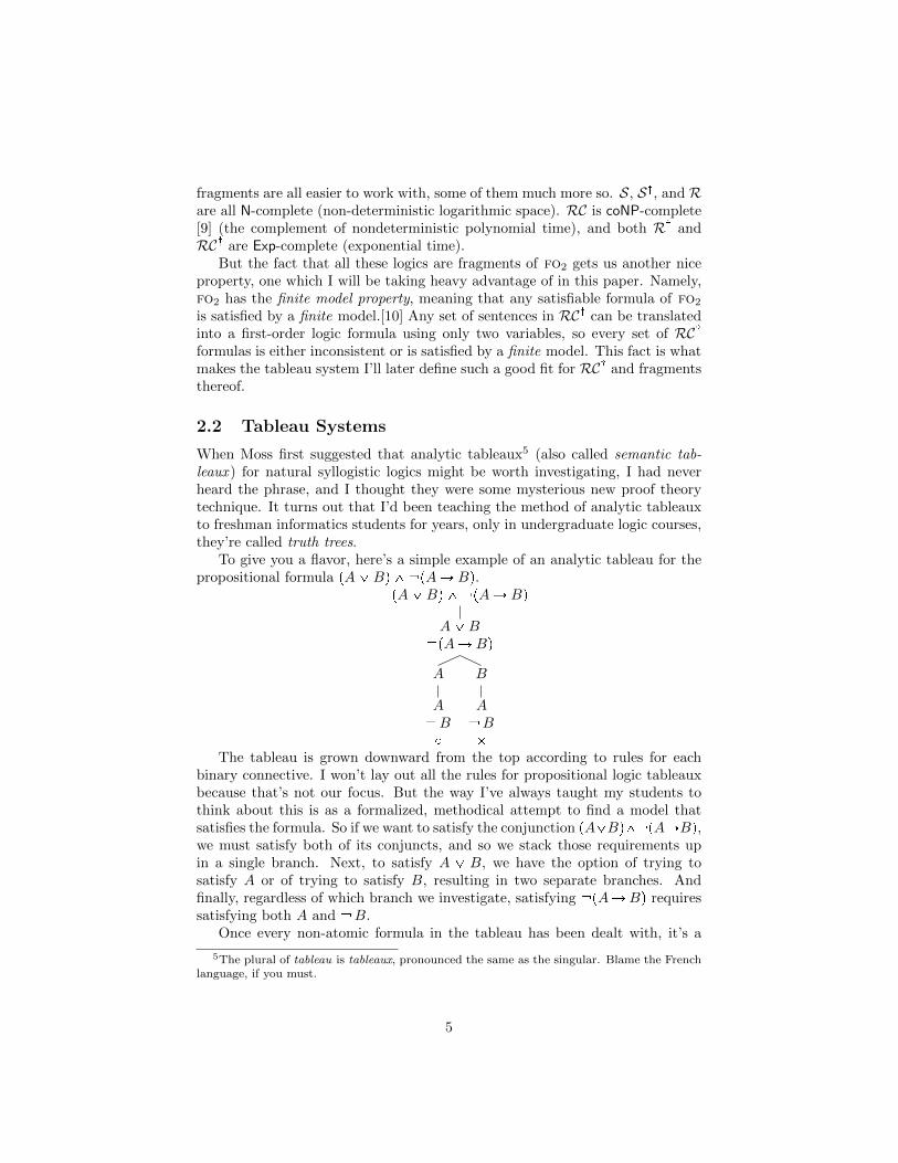
To give you a flavor, here’s a simple example of an analytic tableau for thepropositional formula pA_Bq ^ pAÑBq.

pA_Bq ^ pAÑBq

A_B pAÑBq

A

A B�

B

A B�

The tableau is grown downward from the top according to rules for eachbinary connective. I won’t lay out all the rules for propositional logic tableauxbecause that’s not our focus. But the way I’ve always taught my students tothink about this is as a formalized, methodical attempt to find a model thatsatisfies the formula. So if we want to satisfy the conjunction pA_Bq^ pAÑBq,we must satisfy both of its conjuncts, and so we stack those requirements upin a single branch. Next, to satisfy A _ B, we have the option of trying tosatisfy A or of trying to satisfy B, resulting in two separate branches. Andfinally, regardless of which branch we investigate, satisfying pAÑBq requiressatisfying both A and B.

Once every non-atomic formula in the tableau has been dealt with, it’s a

5The plural of tableau is tableaux, pronounced the same as the singular. Blame the Frenchlanguage, if you must.

5

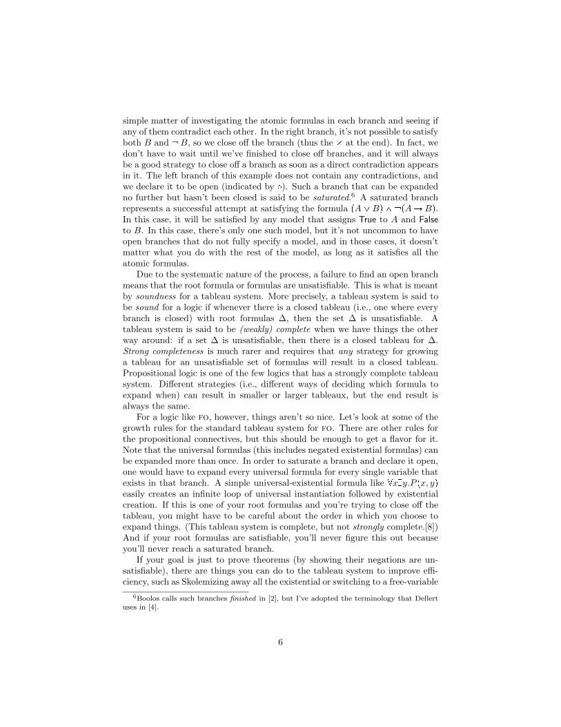
simple matter of investigating the atomic formulas in each branch and seeing ifany of them contradict each other. In the right branch, it’s not possible to satisfyboth B and B, so we close off the branch (thus the � at the end). In fact, wedon’t have to wait until we’ve finished to close off branches, and it will alwaysbe a good strategy to close off a branch as soon as a direct contradiction appearsin it. The left branch of this example does not contain any contradictions, andwe declare it to be open (indicated by �). Such a branch that can be expandedno further but hasn’t been closed is said to be saturated.6 A saturated branchrepresents a successful attempt at satisfying the formula pA_Bq ^ pAÑBq.In this case, it will be satisfied by any model that assigns True to A and Falseto B. In this case, there’s only one such model, but it’s not uncommon to haveopen branches that do not fully specify a model, and in those cases, it doesn’tmatter what you do with the rest of the model, as long as it satisfies all theatomic formulas.

Due to the systematic nature of the process, a failure to find an open branchmeans that the root formula or formulas are unsatisfiable. This is what is meantby soundness for a tableau system. More precisely, a tableau system is said tobe sound for a logic if whenever there is a closed tableau (i.e., one where everybranch is closed) with root formulas ∆, then the set ∆ is unsatisfiable. Atableau system is said to be (weakly) complete when we have things the otherway around: if a set ∆ is unsatisfiable, then there is a closed tableau for ∆.Strong completeness is much rarer and requires that any strategy for growinga tableau for an unsatisfiable set of formulas will result in a closed tableau.Propositional logic is one of the few logics that has a strongly complete tableausystem. Different strategies (i.e., different ways of deciding which formula toexpand when) can result in smaller or larger tableaux, but the end result isalways the same.

For a logic like fo, however, things aren’t so nice. Let’s look at some of thegrowth rules for the standard tableau system for fo. There are other rules forthe propositional connectives, but this should be enough to get a flavor for it.Note that the universal formulas (this includes negated existential formulas) canbe expanded more than once. In order to saturate a branch and declare it open,one would have to expand every universal formula for every single variable thatexists in that branch. A simple universal-existential formula like @xDy.P px, yqeasily creates an infinite loop of universal instantiation followed by existentialcreation. If this is one of your root formulas and you’re trying to close off thetableau, you might have to be careful about the order in which you choose toexpand things. (This tableau system is complete, but not strongly complete.[8])And if your root formulas are satisfiable, you’ll never figure this out becauseyou’ll never reach a saturated branch.

If your goal is just to prove theorems (by showing their negations are un-satisfiable), there are things you can do to the tableau system to improve effi-ciency, such as Skolemizing away all the existential or switching to a free-variable

6Boolos calls such branches finished in [2], but I’ve adopted the terminology that Dellertuses in [4].

6

Figure 1: Tableau Rules for fo

@x.P pxq

P ptq

for existing term t

@x.P pxq

P pcq

for new variable c

Dx.P pxq

P pcq

for new variable c

Dx.P pxq

P ptq

for existing term t

tableau system. But these methods don’t really help with model generation, so Iwon’t be adopting them in this paper. I will try to create systems and strategiesthat terminate when there are no models, but they may not do so very quickly.

The tableau rules that I will introduce for RC: in section 3 are similar to whatyou’d get if you translated each RC: formulas into fo and then expanded theformula according to tableau rules for fo. But since my primary goal is modelgeneration, the existential rule is modified to take advantage of the branchingnature of tableaux to try and find finite models. The existential rule has severalbranches, each one investigating a different candidate for the existential variablein question. There are branches for each of the variables that already exist inthe branch plus an extra branch considering the possibility that a new constantvariable is required. While I believe that such a technique is novel in the contextof natural logics, a very similar method for fo was proposed by John Burgessand proven to always find finite models for fo formulas when they exist byBoolos.[2]

3 A Tableau System for RC:

The nodes in these tableaux consist of a list of variables followed by an RC:predicate of the appropriate arity. In the case of RC: formulas (which arenullary predicates), I will usually just omit the (empty) list. The rules forgrowing tableaux can be phrased in terms of natural language fragments, butadopting the abbreviated notation described in section 2.1 makes them mucheasier to write down. In these rules, σ is a (possibly empty) list of variables.(σ, x is meant to be read as a concatenation of the item x on to the list σ, so if σis the empty list, σ, x is just x.) If we’re dealing with S or S:, σ will always beempty, and in the case of R, R:, RC, and RC:, σ will either be empty or unary.Two-element lists are possible, but only as literals (e.g., x, y : r or x, y : r).The overline notation for the negation of atoms is extended to more complexpredicates in the natural way: @pp, qq :� Dpp, qq and Dpp, qq :� @pp, qq.

In case the bare definitions are a little confusing, I’ll share how I think aboutthem. Suppose we’re set to expand the formula x : @pp, seeq for the existingvariable y. This formula essentially says that x sees all p. So either y is anon-p (represented by the left branch y : p) or x sees y (represented by the rightbranch x, y : see). For the existential rule, suppose we’re expanding the formulax : Dpp, seeq, which says that x sees some p. If y1, . . . , yn is the list of all the

7

Figure 2: Tableau Rules for RC:

σ : @pp, qq

y : p σ, y : q

for existing variable y

σ : Dpp, qq

y1 : pσ, y1 : q

y2 : pσ, y2 : q

� � � yn�1 : pσ, yn�1 : q

where y1, . . . , yn are all of the existingvariables and yn�1 is a new variable

variables that exist in the branch so far, then either one of those yi’s serves asthe p that x sees (resulting in the formulas yi : p and x, yi : see) or none ofthem do, and it’s some new yn�1 that is the p that x sees.

It will be useful to extend the semantics to deal with the variables used inthe tableaux. An extended model M� � xM, v�wy is an ordinary RC: modelwith its denotation map v�w extended to assign each variable to an element ofM . Semantic entailment is also extended. For a model M�, a variable x and aunary predicate p, M� |ù x : p when vxw P vpw, and or a model M�, variablesx and y and a binary predicate r, M� |ù x, y : r when

@vxw , vyw

DP vrw.

Theorem 3.1 (Soundness). Given a set ∆ of RC: formulas, if there is a closedtableau with root formulas ∆, then ∆ is unsatisfiable.

Proof. Suppose that we have a closed tableau with root formulas ∆, but ∆ issatisfied by some model M � xM, v�wy. I will find a contradiction by show-ing that there is some branch of the tableau whose every node is satisfied bythe model M� (where M� is an extension of the model M). This is Lemma3.2. Since the tableau is closed and therefore the branch contains contradictorynodes, this is impossible.

Lemma 3.2. Given a set of RC: formulas ∆ satisfied by some model M �xM, v�wy and a tableau with with root formulas ∆, there is a branch of the tableauand an extension M� of M such that Mx satisfies every node in the branch.

Proof. We inductively extend the model M to M�, simultaneously determiningwhich branch it will satisfy. By assumption, M |ù ∆, so M satisfies all the rootformulas. Suppose we have partially defined M� up to a point, so that vxw isdefined for every constant variable x that has appeared so far, and so that itsatisfies every node of the branch so far. There are several (four, to be precise)cases, depending on whether the next rule applied is a universal or existentialformula, and depending on how many variables are in the formula. I will provetwo of the cases explicitly; the rest are very similar.

Suppose we expand the formula c : @pp, rq for the variable d. By assumptionM� |ù c : @pp, rq, so we know that vcw P v@pp, rqw, and so for all y P vpw, weknow that

@vcw , y

DP vrw. If vdw R vpw, then M� |ù d : p, and we move to the left

8

branch. Otherwise, we must have that@vcw , vdw

DP vrw, and so M� |ù c, d : r

and we move to the right branch.Now let’s consider an existential case. Suppose we expand the formula c :

Dpp, rq and we have existing variables d1, . . . , dn. Since M� |ù c : Dpp, rq, so weknow that vcw P vDpp, rqw, i.e., there is some y P vpw with

@vcw , y

DP vrw. We

might be able to pick one of the branches using old variables, but we don’t needto. Instead we can always move along the rightmost branch, which introducesthe new constant variable dn�1. We define vdwn�1 :� y and so we have thatM� |ù dn�1 : p and M� |ù c, dn�1 : r.

If the model M is a finite model, than we can actually guarantee that theextension M� satisfies every node in a finite branch of the tableau. We simplyfollow the above strategy until there are as many existing variables (d1, . . . , dn)as the size of the model |M |. After that point, when we come to an existentialrule, the pigeonhole principle ensures that we no longer have to choose the right-most branch. One of the branches that reuses a constant variable is acceptable.Since the branch we are on no longer introduces new variables, there are onlyfinitely many formulas and formula-variable pairs to expand and eventually, thebranch will be saturated. This last property is what Boolos calls being completefor finite satisfiability, in contrast to the standard notion of completeness, whichhe calls being complete for unsatisfiability.7

Theorem 3.3. Given a set of RC: formulas ∆ satisfied by some finite modelM � xM, v�wy and a tableau with with root formulas ∆, there is a finite branchof the tableau and an extension M� of M such that Mx satisfies every node inthe branch.

This is a strong result in that it doesn’t matter in what order the formulas arechosen to grow the tableau. If the formulas are finitely satisfiable, any breadth-first search will uncover a finite model in a finite amount of time. Given thatRC: has the finite model property, any breadth-first tableau strategy will provea satisfiable set of formulas to be satisfiable in a finite amount of time. However,depending on the growth strategy, unsatisfiable formulas can result in infinitetableaux.

3.1 Completeness and the Fifo Strategy

The tableau system is strongly complete for S and S:. Infinite branches are im-possible because the only formulas introduced by growth rules in S: are literals(which can’t be expanded any further). So once you’ve expanded all the exis-tential root formulas, there are no new variables, and so there are only finitelymany variables to be expanded for each of the universal formulas. Eventually,every branch will either be closed or saturated. But for the relational frag-ments like RC:, or even R, we aren’t so lucky. Consider the set of formulas

∆ �!@�p, Dpp, rq

�, Dpp, pq,@pp, pq

). Clearly this set is unsatisfiable due to the

7To me, the property seems to have more in common with soundness than completeness.

9

last two formulas, but a willfully obtuse growth strategy can result in an infinitetableau. (I’ve named the constant variable introduced by the nth formula in abranch cn.)

@�p, Dpp, rq

�Dpp, pq@pp, pq

c2 : pc2 : p

c2 : p�

c2 : Dpp, rq

c2 : pc2, c2 : r

...�

c6 : pc2, c6 : r

c6 : p�

c6 : Dpp, rq

c2 : pc6, c2 : r

...�

c6 : pc6, c4 : r

...�

c9 : pc6, c9 : r

. . .

But fortunately, we can be smarter about our growth strategy. There arestrategies that will always result in either a closed tableau or at least one fi-nite open branch. There are two aspects to a tableau-growing strategy: decid-ing which branch to grow and within each branch, deciding which formula (orformula-variable pair8) to expand.

In order to make it easier to prove things about the strategies, I will introducethe notion of an RC: Hintikka set.9 Typically, a Hintikka set for a logic is a(potentially infinite) set of formulas for that logic that are maximally consistentin a particular way. Hintikka sets are often used as a stepping stone for provingcompleteness for a variety of proof systems, especially tableau systems.10 Formy purposes, the members of the Hintikka set will be pairs of a list of variablesand a formula, just like the nodes of the tableau. This essentially includesformulas of RC: (in the form of an empty list paired with a formula), but it alsoincludes things like x : @pa, seeq and x, y : hate. For any such set of pairs H, let

8The existential formulas are each expanded only once, but each universal formula can beexpanded for every constant variable. To keep my sentences from becoming too bloated, whenthe meaning is clear from context, I will sometimes write just “formulas,” even though I reallymean “formulas and formula-variable pairs.”

9I’m still not sure exactly how much “easier” things get with Hintikka sets, but it’s certainlythe traditional way to do it, and I don’t feel like rocking the boat on this one.

10See [5] for examples involving propositional and first-order logic.

10

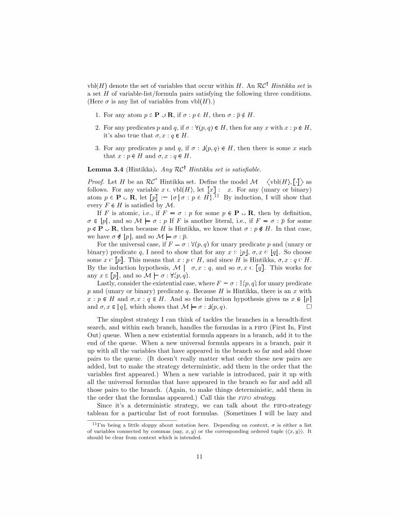
vblpHq denote the set of variables that occur within H. An RC: Hintikka set isa set H of variable-list/formula pairs satisfying the following three conditions.(Here σ is any list of variables from vblpHq.)

1. For any atom p P PYR, if σ : p P H, then σ : p R H.

2. For any predicates p and q, if σ : @pp, qq P H, then for any x with x : p P H,it’s also true that σ, x : q P H.

3. For any predicates p and q, if σ : Dpp, qq P H, then there is some x suchthat x : p P H and σ, x : q P H.

Lemma 3.4 (Hintikka). Any RC: Hintikka set is satisfiable.

Proof. Let H be an RC: Hintikka set. Define the model M �@vblpHq, v�w

Das

follows. For any variable x P vblpHq, let vxw :� x. For any (unary or binary)atom p P P Y R, let vpw :� tσ |σ : p P Hu.11 By induction, I will show thatevery F P H is satisfied by M.

If F is atomic, i.e., if F � σ : p for some p P P Y R, then by definition,σ P vpw, and so M |ù σ : p If F is another literal, i.e., if F � σ : p for somep P P YR, then because H is Hintikka, we know that σ : p R H. In that case,we have σ R vpw, and so M |ù σ : p.

For the universal case, if F � σ : @pp, qq for unary predicate p and (unary orbinary) predicate q, I need to show that for any x P vpw, σ, x P vqw. So choosesome x P vpw. This means that x : p P H, and since H is Hintikka, σ, x : q P H.By the induction hypothesis, M |ù σ, x : q, and so σ, x P vqw. This works forany x P vpw, and so M |ù σ : @pp, qq.

Lastly, consider the existential case, where F � σ : Dpp, qq for unary predicatep and (unary or binary) predicate q. Because H is Hintikka, there is an x withx : p P H and σ, x : q P H. And so the induction hypothesis gives us x P vpwand σ, x P vqw, which shows that M |ù σ : Dpp, qq.

The simplest strategy I can think of tackles the branches in a breadth-firstsearch, and within each branch, handles the formulas in a fifo (First In, FirstOut) queue. When a new existential formula appears in a branch, add it to theend of the queue. When a new universal formula appears in a branch, pair itup with all the variables that have appeared in the branch so far and add thosepairs to the queue. (It doesn’t really matter what order these new pairs areadded, but to make the strategy deterministic, add them in the order that thevariables first appeared.) When a new variable is introduced, pair it up withall the universal formulas that have appeared in the branch so far and add allthose pairs to the branch. (Again, to make things deterministic, add them inthe order that the formulas appeared.) Call this the FIFO strategy.

Since it’s a deterministic strategy, we can talk about the fifo-strategytableau for a particular list of root formulas. (Sometimes I will be lazy and

11I’m being a little sloppy about notation here. Depending on context, σ is either a listof variables connected by commas (say, x, y) or the corresponding ordered tuple (xx, yy). Itshould be clear from context which is intended.

11

talk about the fifo-strategy tableau for a set of root formulas, in which caseyou can just assume that there’s a particular order on that set.) The fifostrategy can have infinite branches, but only if the root formulas are satisfiable,and even then, it will always have a finite open branch. The reason for this isthat every open branch (this includes any infinite branches) of a tableau grownusing the fifo strategy can be used to produce a model.

Lemma 3.5 (The Fifo Strategy). Given any non-closed branch of the fifo-strategy tableau for a set of root formulas ∆, there is a model M �

@M, v�w

Dthat satisfies every node in the branch (in particular, M |ù ∆).

Proof. There’s not much to the proof here. It’s mostly a matter of showing thatthe nodes of the branch form an RC: Hintikka set. Since it’s not closed, it clearlysatisfies the first condition. Due to the first-in/first-out nature of the queue andbecause at every step, only finitely many formulas are added to the queue, everyformula and formula-variable pair is eventually expanded in the branch. Theexpansion rules make sure that the second and third Hintikka conditions arealso met. So the Hintikka Lemma gives us the model we need.

If you follow the fifo strategy, even infinite branches yield models, so everybranch of a tableau with unsatisfiable root formulas must eventually be closedoff. That gives us the following theorem.

Theorem 3.6 (RC: Completeness). Every unsatisfiable set of RC: formulashas a closed tableau.

Theorems 3.3 and 3.6 together imply that the fifo strategy can be usedas an algorithm to determine the satisfiability of any set of RC: formulas in afinite amount of time. Simply follow the strategy and if the tableau closes off,the set is unsatisfiable. If it doesn’t close off, it will eventually produce a finite,saturated branch which can be used to easily generate a finite model.

3.2 Other Strategies

The fifo strategy is a relatively naıve strategy, but it suits the purpose ofproving the existence of an algorithm for deciding RC: satisfiability that alsoprovides finite models. But there are some things that can be done to speedthings up, at least in some cases. There are two things we can adjust. Thefirst is how we decide which formula to expand next in each branch (that’sthe fifo part of the fifo strategy). We can speed things up here by eitherattempting to get contradictions earlier (allowing us to close off branches) orby pushing the more heavily branching rules further down the tableau (creatingless redundancy). The danger with adjusting this order is that you can ruincompleteness (for unsatisfiability) by creating a situation where some formulanever gets expanded (because it keeps getting pushed further down the queue).

In the RC: tableaux I’ve defined in this article, universal expansion rulesalways produce two branches, but after the first two of variables are intro-duced, existential rules always produce more than two branches. So we can try

12

to eliminate some redundancy by taking care of all universal expansion stepsbefore expanding any existential formulas. I call this the universal-first strat-egy. Fortunately, this strategy does not ruin completeness, provided we takea first-in/first-out approach once we do decide to tackle an existential formula.The reason is that universal expansion rules never introduce any new variables.There are only finitely many nodes that can ever be introduced using the finiteset of formulas, predicates, and variables that already exist inside the branch.

A more complex approach is to try to close off branches as soon as possible.One way to do this is to give priority to expanding any universal formula-variablepair where one of the resulting two branches will immediately be closed off. Forexample, the expansion of the formula @

�p, Dpq, seeq

�for the variable c would

produce a branch with the node c : p, so if c : p is already in the branch, thisexpansion should be moved to the front of the queue. I call this the immediateclosure strategy. As long as you stick to moving universal expansions up in thequeue and don’t move the existential formulas down in the queue, completenessis assured.

The second thing that we can adjust is the way in which we decide whichbranch to work on. This doesn’t affect the tableau we’re growing, but it canaffect the order in which we find finite models, and if the tableau has infinitebranches, it can change whether we find them at all. Obviously, a depth-firstsearch is a bad idea when there might be infinite branches. But there areother options. For example, if we’re interested in finding the smallest possiblefinite model, then instead of taking a pure breadth-first search pattern, we canprioritize branches based on the number of constant variables that appear inthem. More precisely, we postpone growing the rightmost branches of existentialexpansion steps (those’re the one that introduce new variables) until after we’veexpanded along every other branch. This means that all possible size-n modelswill be investigated before we even consider any size n � q models. I call thisa model-size-tiered search. Within the model-size tiers, we can use any searchmethod, including depth-first, without worrying about getting stuck working onan infinite branch. This is because any infinite branch must necessarily containinfinitely many constant variables.

4 RC-tabModG: an Implementation

RC-tabModG12 (Tableau-based Model Generator) is my implementation ofthis tableau system in MiniKanren, a relational programming system embeddedin Scheme.13 One reason I chose MiniKanren was to take advantage of itscondeoperator, which effectively allows the program to investigate each branchof the tableau more or less in parallel. This sidesteps the issue of deciding whichbranch to grow when, which doesn’t affect the tableau being grown, only in whatorder we grow it. This puts the focus on the other aspects of strategy, which doaffect what tableau we’ll end up with. The other big reason is that choosing a

12Pronounced “R-C-tab-modge”.13Check out [3] or [6] for good introductions to MiniKanren.

13

relational language like MiniKanren allows the program to do things other thanjust taking formulas and grow tableaux, such as taking existing tableaux andverifying their correctness.

RC-tabModG is related to αleantap by Near, Byrd, and Friedman [12] inthat it is also a tableau-based theorem prover implemented in MiniKanren,but they are put together quite differently. αleantap is a theorem prover forfirst-order logic, a descendant of leantap, a tableau-based theorem prover inProlog.[1] As theorem provers, neither of these produce countermodels, andthe difference in focus means that they take an entirely different approach totableaux.

I won’t be giving explicit details of the implementation here, but I’ll describethings in general. Source code is available upon request. But a few words aboutMiniKanren are called for before I start talking about RC-tabModG.

It’s a tradition in MiniKanren to add the suffix -o to the names of relationaloperators (which attempt to create a relation between inputs), to distinguishthem from standard Scheme operators (which have an input and an output).So while the traditional Scheme operator car takes a list as input and outputsthe object that is at the head of the list, the MiniKanren relation caro has twoinputs (a list and an object) and tries to ensure that that the object (the secondinput) is the head of the list (the first input). When the first input is fullyspecified (meaning that we give an actual list) and the second is left unspecified(because it’s a variable created by the Scheme operator lambda or one of theMiniKanren operator fresh or run), we say that caro is being run forwards. Inthat case, caro will succeed, and will identify the first member of the list withthe variable given for the second input. If the first input is left unspecified, butthe second input is fully specified, then we call this running backwards, and caro

will succeed, with the result being that the first input is now partially specifiedas a list with the second input as its head and an unspecified tail. If bothinputs are all or partially specified, then caro may succeed or fail, depending onwhether it’s possible to unify the head of the first input with the second input.

The relational operators of MiniKanren (like caro) are typically called us-ing the run operator, which attempts to make all the necessary unificationsand assigns names to all the variables that remain unspecified at the end ofthe process. Many relations can succeed in a variety of ways. For example,the membero relation might succeed because the second argument is the firstmember of the first argument, or because it’s the second member of the firstargument, or because it’s the third. . . So the run operator takes a number asone of its arguments, indicating how many different answers are desired. There’salso a run* version that returns a list of all possible answers, but in many un-derspecified cases, the process will never terminate, as MiniKanren will neverrun out of possibilities to try.

Most of the functionality of RC-tabModG is in the growo relation, whichrelates a list of the formulas in a (usually partial) branch (the branch-so-far),a list of the formulas (and formula-variable pairs) that still need to be expanded,and a list of the variables that have already appeared to a list of the formulasthat have yet be added to the branch (the branch-to-be). When running in

14

the forward direction, this last list of formulas yet to be added is left unspecifiedby the user and is filled in by MiniKanren.

We could also specify the entire branch-to-be and ask it to verify that itwas grown correctly according to the strategy specified. Theoretically, we couldalso specify all or part of the branch-to-be and ask MiniKanren to give usall or part of the branch-so-far, but it’s difficult to think of good ways tomake use of that in practice. Perhaps if you were trying to find a model fora set of formulas and most of the models produced were degenerate in someway, you could specify some extra properties for the branch-to-be to cull outundesirable branches.

Of course, there are usually many different ways of filling in the rest of thebranch, and this is where the conde operator is useful. The code doesn’t specifywhich branch will fill out the branch-to-be, but it does specify what formulaswill appear in each of the possible branches as different conde cases. If askedfor a certain number of branches, MiniKanren will keep growing branches inparallel until it has enough branches that are complete (either closed or finiteand saturated (and therefore open)), or until every branch is complete, evenif there aren’t enough. If asked for all branches, it will keep going until everybranch is complete. This is usually a bad idea, however, as many tableaux willhave infinite branches, and so the process will never terminate.

Usually, the user won’t interact with growo directly, instead using either thebrancho or open-brancho relations, which will fill in the unexpanded formulasand variables automatically before calling growo . In the case of open-brancho ,the closed branches will be filtered out. It’s a simple matter to read off asatisfying model from an open branch, but the relation modelo will do that foryou, if you’re feeling lazy. Similarly, if you’d like the program to print all orpart of a tree instead of a list of branches, you can use the impure operatorgrow-tableau. Both modelo and grow-tableau also do some cleaning up to makethings more readable.14

4.1 Performance

Currently, I have implemented three versions of RC-tabModG, one implement-ing the fifostrategy, one implementing the universal-first (uf) strategy, and oneimplementing both the universal-first and the immediate-closure (ufic) strate-gies. As far as I know, there are no standard sets of RC: formulas for testingperformance, but I have compared runtimes and memory requirements for find-ing models for a few hand-selected sets of RC: formulas, some of which I havepresented here. This data is from running Petite Chez Scheme on a laptop15

running Windows 7 (64 bit), so the time comparisons are really only relevantwhen compared to each other. The number (“one” or “ten”) represents howmany models I asked RC-tabModG to generate. In the case of S2, there arefewer than 10 branches in the complete tree, so I just asked for all of them.

14The default is to name new variables after the formula which generated them, but thiscan be confusing to read, so these operators rename the variables using numbered indices.

15If you must know, it’s a Samsung Notebook with a 2.20 GHz Intel i7 cpu and 6 GB ram.

15

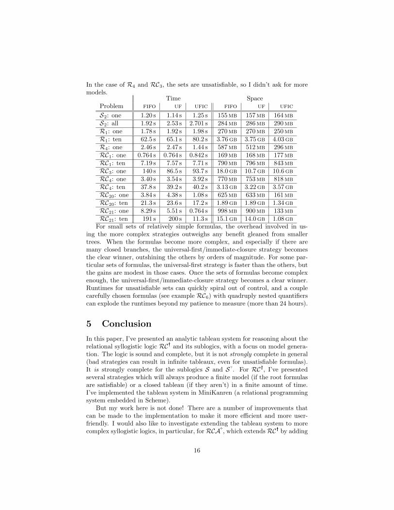
In the case of R4 and RC3, the sets are unsatisfiable, so I didn’t ask for moremodels.

Time SpaceProblem fifo uf ufic fifo uf ufic

S2: one 1.20 s 1.14 s 1.25 s 155mb 157mb 164mbS2: all 1.92 s 2.53 s 2.701 s 284mb 286mb 290mbR1: one 1.78 s 1.92 s 1.98 s 270mb 270mb 250mbR1: ten 62.5 s 65.1 s 80.2 s 3.76gb 3.75gb 4.03gbR4: one 2.46 s 2.47 s 1.44 s 587mb 512mb 296mbRC1: one 0.764 s 0.764 s 0.842 s 169mb 168mb 177mbRC1: ten 7.19 s 7.57 s 7.71 s 790mb 796mb 843mbRC3: one 140 s 86.5 s 93.7 s 18.0gb 10.7gb 10.6gbRC4: one 3.40 s 3.54 s 3.92 s 770mb 753mb 818mbRC4: ten 37.8 s 39.2 s 40.2 s 3.13gb 3.22gb 3.57gbRC20: one 3.84 s 4.38 s 1.08 s 625mb 633mb 161mbRC20: ten 21.3 s 23.6 s 17.2 s 1.89gb 1.89gb 1.34gbRC21: one 8.29 s 5.51 s 0.764 s 998mb 900mb 133mbRC21: ten 191 s 200 s 11.3 s 15.1gb 14.0gb 1.08gb

For small sets of relatively simple formulas, the overhead involved in us-ing the more complex strategies outweighs any benefit gleaned from smallertrees. When the formulas become more complex, and especially if there aremany closed branches, the universal-first/immediate-closure strategy becomesthe clear winner, outshining the others by orders of magnitude. For some par-ticular sets of formulas, the universal-first strategy is faster than the others, butthe gains are modest in those cases. Once the sets of formulas become complexenough, the universal-first/immediate-closure strategy becomes a clear winner.Runtimes for unsatisfiable sets can quickly spiral out of control, and a couplecarefully chosen formulas (see example RC6) with quadruply nested quantifierscan explode the runtimes beyond my patience to measure (more than 24 hours).

5 Conclusion

In this paper, I’ve presented an analytic tableau system for reasoning about therelational syllogistic logic RC: and its sublogics, with a focus on model genera-tion. The logic is sound and complete, but it is not strongly complete in general(bad strategies can result in infinite tableaux, even for unsatisfiable formulas).It is strongly complete for the sublogics S and S:. For RC:, I’ve presentedseveral strategies which will always produce a finite model (if the root formulasare satisfiable) or a closed tableau (if they aren’t) in a finite amount of time.I’ve implemented the tableau system in MiniKanren (a relational programmingsystem embedded in Scheme).

But my work here is not done! There are a number of improvements thatcan be made to the implementation to make it more efficient and more user-friendly. I would also like to investigate extending the tableau system to morecomplex syllogistic logics, in particular, for RCA:, which extends RC: by adding

16

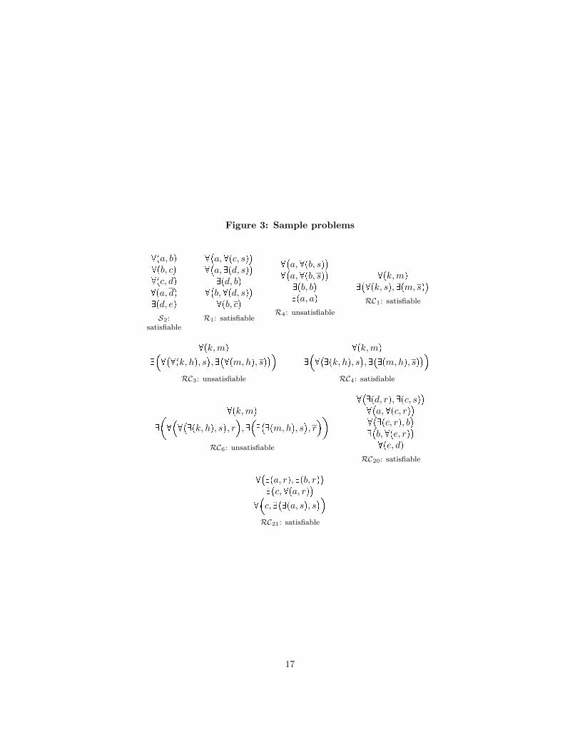
Figure 3: Sample problems

@pa, bq@pb, cq@pc, dq@pa, dqDpd, eq

S2:satisfiable

@�a,@pc, sq

�@�a, Dpd, sq

�Dpd, bq

@�b,@pd, sq

�@pb, cq

R1: satisfiable

@�a,@pb, sq

�@�a,@pb, sq

�Dpb, bqDpa, aq

R4: unsatisfiable

@pk,mqD�@pk, sq, Dpm, sq

�RC1: satisfiable

@pk,mq

D�@�@pk, hq, s

�, D�@pm,hq, sq

�RC3: unsatisfiable

@pk,mq

D�@�Dpk, hq, s

�, D�Dpm,hq, sq

�RC4: satisfiable

@pk,mq

D

�@�@�Dpk, hq, s

�, r, D�D�Dpm,hq, s

�, r

RC6: unsatisfiable

@�Dpd, rq, Dpc, sq

�@�a,@pc, rq

�@�Dpc, rq, b

�D�b,@pe, rq

�@pe, dq

RC20: satisfiable

@�Dpa, rq, Dpb, rq

�D�c,@pa, rq

�@�c, D

�Dpa, sq, s

�RC21: satisfiable

17

comparative adjectives, which are automatically transitive and reflexive. RCA:

does not have the finite model property, and I would like to investigate tableau-based strategies for identifying repeating patterns in infinite branches with theintent of finding infinite models in a finite amount of time.

References

[1] Bernhard Beckert and Joachim Posegga. leantap: Lean tableau-based de-duction. Journal of Automated Reasoning, 15(3):339–358, 1995.

[2] George Boolos. Trees and finite satisfiability: proof of a conjecture ofburgess. Notre Dame Journal of Formal Logic, 25(3):193–197, 1984.

[3] William E Byrd. Relational programming in MiniKanren: techniques, ap-plications, and implementations. PhD thesis, Indiana University Bloom-ington, 2010.

[4] Johannes Dellert. Challenges of model generation for natural languageprocessing. Master’s thesis, University of Tubingen, 2011.

[5] Melvin Fitting. First-Order Logic and Automated Theorem Proving. Grad-uate Texts in Computer Science. Springer, second edition, 1996.

[6] Daniel P Friedman, William E Byrd, and Oleg Kiselyov. The ReasonedSchemer. The MIT Press, second edition, 2006.

[7] Erich Gradel, Phokion G Kolaitis, and Moshe Y Vardi. On the decisionproblem for two-variable first-order logic. Bulletin of symbolic logic, pages53–69, 1997.

[8] Reiner Hahnle. Tableaux and related methods. Handbook of automatedreasoning, 1:101–178, 2001.

[9] David A McAllester and Robert Givan. Natural language syntax and first-order inference. Artificial Intelligence, 56(1):1–20, 1992.

[10] Michael Mortimer. On languages with two variables. Mathematical LogicQuarterly, 21(1):135–140, 1975.

[11] Reinhard Muskens. An analytic tableau system for natural logic. In Logic,Language and Meaning, pages 104–113. Springer, 2010.

[12] Joseph P Near, William E Byrd, and Daniel P Friedman. αleantap: Adeclarative theorem prover for first-order classical logic. In Logic Program-ming, pages 238–252. Springer, 2008.

[13] Ian Pratt-Hartmann and Lawrence S Moss. Logics for the relational syllo-gistic. The Review of Symbolic Logic, 2(04):647–683, 2009.

18