table of contents - signal processing systems...
TRANSCRIPT
PTDCEEA-TEL679792006 - PLC Noise - year 3
Page 1
T A B L E O F C O N T E N T S
Adaptive Impedance and Limits on the Signals ....................................................................................... 4
The radiated signal is proportional to the current ............................................................................ 4
The distribution of the Electric Field Given Measurements .......................................................... 4
The Probability Density of the Positive Wave and Negative Wave Current Given the Input Current ..................................................................................................................................................... 5
The Power Line Graph can be Analyzed as a set of Independent Virtual Transmission Lines (one for each leaf) ............................................................................................................................... 8
The Expected Value of Radiated Field given the Input Current at a narrow band ............... 8
The Improvement Achieved by Using the Input Impedance Estimate .................................... 10
Noise Measurements Circuits ........................................................................................................................ 17
Parasitic Capacitors and inductors ........................................................................................................ 21
A small transmission line ........................................................................................................................... 23
Analysis of the pickup cirCuit ................................................................................................................... 26
Circuit with one and two capacitors ...................................................................................................... 29
Transformer measurements ..................................................................................................................... 29
Analyzing the measurements of the coilcraft WB1-1 ................................................................ 38
Modeling the transformer as a transmission line ....................................................................... 40
Common and differential mode transmission line transformer ........................................... 43
Traditional Balauns circuits ................................................................................................................. 45
Inductors ...................................................................................................................................................... 46
Coilcraft wideband transformer Distortion Measurements ................................................... 47
Amplifier ........................................................................................................................................................... 47
IC Amplifier measurements ................................................................................................................. 47
Typical IC amplifier ................................................................................................................................. 50
Measurements circuit with an IC amplifier ................................................................................... 52
Amplifier distortion ................................................................................................................................. 55
IP3 Point ....................................................................................................................................................... 56
ZFL-500+ Amplifier Measurements ................................................................................................. 57
ZFL-500Ln+ Amplifier Measurements ............................................................................................ 59
Amplifier Noise figure ............................................................................................................................ 59
Power supply noise ................................................................................................................................. 59
pickup circuit ................................................................................................................................................... 64
Anti-aliasing LC Filter .................................................................................................................................. 65
Termination impedance and LISN .......................................................................................................... 66

PTDCEEA-TEL679792006 - PLC Noise - year 3
Page 2
Dealing with the different noise levels ................................................................................................. 67
Relation of the expected noise levels to EMC limits ........................................................................ 68
Measurements with module amplifiers ............................................................................................... 68
Final measurement Setup .......................................................................................................................... 71
Non linearity’s in the channel ........................................................................................................................ 72
Power Line Noise Measurements ................................................................................................................. 72
Analyzing the Noise measurements ............................................................................................................ 83
Estimation of the correlation coefficients matrix of the Received Signal .............................. 83
Sample standard deviation ................................................................................................................... 83
Chebyshev Inequality ............................................................................................................................. 83
Correlation Coefficients ......................................................................................................................... 83
Complex Correlation Coefficients ...................................................................................................... 84
Derivative of RE(X) .................................................................................................................................. 85
Estimating the Correlation Matrix and Correlation Coefficients Matrix ........................... 85
Estimation of the correlation coefficients matrix of the Compensated OFDM signal version one .................................................................................................................................................. 87
Phase Variation With k........................................................................................................................... 94
Estimation of the correlation coefficients matrix of the Compensated OFDM signal version two ................................................................................................................................................. 98
The model for the noise ...................................................................................................................... 106
Noise Generation Model ..................................................................................................................... 108
Estimation of the difference between the autocorrelation and cross-correlation ..... 109
The Modem ......................................................................................................................................................... 110
Removal of Sinusoidal Signals ............................................................................................................... 110
Noise Time Correlation for different OFDM Symbols .................................................................. 110
Estimating the channel transfer function signal to noise ratio and input impedance ... 110
Estimation with impulse noise.............................................................................................................. 110
Channel coding ............................................................................................................................................ 116
MAximum capacity using QAM and the Capacity of a binary channel ............................ 117
Probability of bit error with error correcting ........................................................................... 118
MAP Demodulation .................................................................................................................................... 119
Union Bound ................................................................................................................................................. 119
Quality of Service ........................................................................................................................................ 121
Not So Low Capacity Gap and High Signal to Noise Case ................................................ 121
Channel Estimating Gap ........................................................................................................................... 128
PAM or non-Orthogonal Codes Pilots and Fast Changing Channels ...................................... 129
The Techniques for Impulsive Or BursT noise reduction ............................................................... 129
PTDCEEA-TEL679792006 - PLC Noise - year 3
Page 3
Capacity .......................................................................................................................................................... 130
Capacity with Impulsive Noise .............................................................................................................. 131
Capacity for non-Gaussian signals ....................................................................................................... 133
Codes ................................................................................................................................................................ 136
The Pros and Cons of Adding a new Estimation Parameter ..................................................... 136
Detection of Burst in Signals .................................................................................................................. 137
Dividing the Symbol Length ................................................................................................................... 137
Careful Correlation Estimation ............................................................................................................. 137
Non Gaussian to Non-Stationary Conversion.................................................................................. 138
Minimum Distance Estimator ................................................................................................................ 138
Demodulation with Impulse Noise ...................................................................................................... 138
Power Line Modem Simulator .................................................................................................................... 138
References .......................................................................................................................................................... 140
PTDCEEA-TEL679792006 - PLC Noise - year 3
Page 4
ADAPTIVE IMPEDANCE AND LIMITS ON THE SIGNALS
THE RADIATED SIGNAL IS PROPORTIONAL TO THE CURRENT
The radiated signal is proportional to the current in the line, as in the formulas presented in the previous reports. In an antenna it increases with frequency but only until the antenna length is equal to . Since power lines are very long antennas this limits will be reached rapidly.
THE DISTRIBUTION OF THE ELECTRIC FIELD GIVEN MEASUREMENTS
We have that at the input of the power line will be given by the subtraction of the positive wave minus the negative wave namely,
And
Or,
And
We have that
It was showed that the radiated far field will be related to , since this will be lower that the sum of the positive and negative wave. In short lines this limit may be almost reached, however, the integration length will be shorter, so it is possible that this will be improved (we are still working on it).
The negative wave will always be lower than the positive wave, since its power is lower since it is a reflection and the impedance is the same. The signal can be taken to be real since the only interested value is the electric field magnitude. The value of will be,
Since is the applied voltage, and is known, then is also known. In other to get an distribution for , a distribution for needs to be assumed. In most cases should have a low value, so using a real uniform distribution from to gives a conservative result. A real signal is also not very accurate, but it should give us some insight to the results. So making
| ,

PTDCEEA-TEL679792006 - PLC Noise - year 3
Page 5
Note that is also a sample of the random variable . What is the PDF of ? One has,
PD ∑ PD | PD
Or
PD ∫ PD | PD
And
PD PD
PD ∫PD
And with
PD ∫PD
THE PROBABILITY DENSITY OF THE POSITIVE WAVE AND NEGATIVE WAVE CURRENT GIVEN THE INPUT CURRENT
From file: João Pinto/3_9_10.docx
Given the measurement of , one needs to determine what is the worst case for the expected value of . One will assume that the reflected wave will have a magnitude that is of the transmitted wave. This will result in a standing wave, that is sampled at a given phase, , resulting in,
(PD.1)
With
PD
However, in order to get monotones function it is better to chose
PD

PTDCEEA-TEL679792006 - PLC Noise - year 3
Page 6
Since this will result in the same distribution. Solving the equation to allows calculation of PD | .
Using,
| |
So the result is
See Mathematica file ..\PDIp.nb
This should a function of the type,
|
One can now calculate the expected value for the positive wave current. Note that the expected value is linear with the input current.
In a modem one has an additional information, that is the value of the voltage at the input, , or the input impedance, , this will give us a hint to which point of the standing we are sampling as long as the distribution of the line characteristic impedance is known. If this is not known then the there is probably no extra information given from measurements besides the current, because the radiation level only of the current.
The fact that for instance the value of is never bellow can be incorporated into this formulation and maybe it is possible to guaranty the radiation is under the limits in any case but using a bit higher signals.
Given this formulation the probability density of the positive wave current will be,
√
for
This function is plotted in Figure 1 for and .

PTDCEEA-TEL679792006 - PLC Noise - year 3
Page 7
FIGURE 1 – THE PROBABILITY DENSITY THE POSITIVE WAVE CURRENT FOR A STANDING WAVE WITH A COEFFICIENT AND INPUT CURRENT I=1.
The expected value of the current positive travelling wave current will be a function of , according to the following table.
0.1 0.5 0.6 0.7 0.8 0.9 0.99 0.999 | 1.0050 1.1547 1.2500 1.4003 1.6667 2.2942 7.0888 22.366
TABLE 1 – EXPECTED VALUE OF THE TRANSMITTED WAVE CURRENT AS A FUNCTION OF ALPHA
This is as expected. Not that the expected value of given is equal to , but the expected value of given is not . It will be always greater than depending on as seen in the table. It is zero then they are equal since there is no standing wave. If is one, then can have very high values, because of the division by zero, so the expected value is large, as seen in the table. We can also see that it increases between the two values.
A reasonable assumption may be to assume that the expected value is bellow about , since this requires an of .
Note that usually as a measurement of the characteristics of the standing is used the standing wave ratio, that is equal to the ratio of the maximum of the standing wave to the minimum of the standing wave, and this is equal to,
Finally note that it is still not clear to us what is limited be regulations, if it is the expected value of radiation, or an actual limit for any case. Historically it seems that at least one of the reasons that unintentional radiators were limited was to prevent a phenomenon of large scale integration, were many very far radiators, for instance in china may add up in such a way that the resulting field would be infinite, since the power decreases with but the radios increases with and the integral of is infinite. This means that the field in any given location will be the result of many radiators and that the average value if of most importance, and not the actual value for a specific place.

PTDCEEA-TEL679792006 - PLC Noise - year 3
Page 8
THE POWER LINE GRAPH CAN BE ANALYZED AS A SET OF INDEPENDENT VIRTUAL TRANSMISSION LINES (ONE FOR EACH LEAF)
A power line is a graph, were, the lines are vertices and the terminals leafs. At each line the current can be taken as a sum of currents each corresponding to a virtual line, one for each leaf. Impedance change in the lines can be modeled as new leafs in the middle of the line. This can be proved doing the calculations for each node.
…
In a single line changing the frequency is equivalent to moving along the line, so decomposing the power line in a set of independent lines will allows determine the effect of frequency averages. The speed of the movement with frequency along the stationary wave in each line will depend on the line.
At the end of the transmission one will have a given reflection coefficient so this will determine the point at the standing wave. The point of the standing at the beginning will depend of the line length.
THE EXPECTED VALUE OF RADIATED FIELD GIVEN THE INPUT CURRENT AT A NARROW BAND
To estimate the radiated field, instead of using the input current at a single frequency, it is more reasonable to use the values a narrow band surrounding each frequency. In a more detailed way, the radiated field should be limited for instance in the 30 MHz to the 80MHZ range. In each frequency, like 50 MHz one would use measurements of the current at for instance 49.5 MHz to 50.5 MHz.
In such a short band the amplitudes the reflection coefficient at all leafs should be more or less constant. One would expect that we should have a few poles and zeros corresponding for instance to the model of a transformer, but the distance between them should be related to their frequency, and at 50 MHz the distance should be much greater than 1 MHz.
Changing the measuring frequency is at some extent equivalent to travelling in the standing wave. The speed we travel in the standing wave will be dependent on the line length.
This can be calculated in the following way. If the frequency changes the point we are in the traveling wave at the far end of the line will be the same, but the point at the near end will change. How much the frequency has to change so that the point at the near end moves one standing wave wavelength? It will be when the number of wavelengths inside the line increases by one. Since the standing wave wavelength is half of wave wavelength then we have that, if is the wave wavelength at frequency and is the wave wavelength at frequency , then we should wave,
Or

PTDCEEA-TEL679792006 - PLC Noise - year 3
Page 9
Were is the line length. And since
We get
So changing the frequency by will correspond to travel be in the line, that is changing the frequency by will correspond to moving a distance of . The moving speed will then be,
We can also derive this equations based on the transmission line equations. So we have
With
And
( (
) )
That is the complex amplitude of the wave at a distance from the left edge and at frequency is equal to the complex amplitude of the signal at the edge but a lower frequency. These means that, taking frequency averages will be equal to taking positional averages of the current signal, but the actual position will depend of the virtual line length, , or,
(
)
Or
L L-x 0
FIGURE 2 – POSITION ON THE LINE. THE ZERO IS AT THE RIGHT SINCE THIS WILL ALWAYS BE AT A FIXED POINT IN THE STANDING WAVE, GIVEN THE REFLECTION COEFFICIENT.

PTDCEEA-TEL679792006 - PLC Noise - year 3
Page 10
Taking averages along the line position will help can be done calculating the integral using the above formulas. This will correspond to frequency averages by doing a change in the integration variable. Doing this will reduce the variance of the estimate of the positive wave current or of the radiated field. If the actual limit is due to a very large number of averages as discusses before, this may not be very important, since the variance will be very low. But if we are aiming to do something like the radiated field can only pass a given limit in 1% of the cases, then the variance of the estimate will be important.
We have already calculated the expected value of the estimate we need also to calculate the variance, and we can do it taking into account frequency averages.
We are interested in calculating the variance of the estimate,
∫
This will be equal to,
∫ ( (
) )
(
)
(
)
With
(
)
Doing the variables change results in
∫
(
)
(
)
If the frequency interval considered is small then we still have,
(
)
(∫
)
(∫
)
With
This is the same formula as above. Not forgetting that we are trying to calculate the average value of the amplitude of the standing wave, the actual variance will probably depend on the percentage of the standing wave we have covered, that is,
(
) (
)
We do not know the actual line length but we could use a worst case scenario…….
THE IMPROVEMENT ACHIEVED BY USING THE INPUT IMPEDANCE ESTIMATE

PTDCEEA-TEL679792006 - PLC Noise - year 3
Page 11
In year 2 report is was shown that (to be rechecked and summarized),
| | |
|
And we also have that for a long line with low attenuation the expected value of should be equal to , since the current will fluctuate around it, and
| | | |
(Maybe this should be done for the expected power!!! )
Using the formula
values for I can be calculated from E as in the excel file bellow, namely,
F (MHz) E, classe B (V/m) Norma r Banda (Hz) Z0 (Ohm) LCL (dB) I=4 pi E r/Z0/Sqrt(B)*10^(LCL/20) (A/Sqrt(Hz))
30-230 1,00E-04 FCC 3,00 120.000,00 376,73 36,00 1,82E-06
√
The maximum for the voltage was derived, given by,
And
The actual value for the line impedance is unknown, but a worst case value could be used, let’s say . This will be one of the techniques.
We will have two models: Model one is a line with characteristic impedance (Z) distribution and a limit for the values of Z. Model two is a line with an and p distribution.
The distribution of p is uniform between – and . Knowing the distribution of p is the advantage of this model. The value of is limited. Other models could be using a experimentally determined distribution for Z or .
We proceed to determine how to calculate the value of the transmitted wave current for model 2.
The voltage at input of the line is and the transmitted current wave amplitude is , the reflected is , the line impedance is and the access impedance is and the access voltage is . Writing the equations for the transmission line at the input one has,

PTDCEEA-TEL679792006 - PLC Noise - year 3
Page 12
Solving this eliminating and results in
Using (PD.1) namely
Results in
Or
And still
Defining a reflection coefficient at the emitter, , as
The reflection coefficient at the emitter side that relates the negative wave with the component of the positive that is due to reflections instead of transmissions. Note that this is totally independent from and since this can only be determined from the reflection coefficient at the receiver . (R close zero the reflection coefficient is -1 and the voltage will be zero)
This will simplify the formula and we get a constant, , multiplied by , resulting in
(
)
But we are still going to use the other formula so that the relation between both formulas is more obvious.
We can see that the fact that is unknown in this implied that and are required to be added to the model. (link)
PTDCEEA-TEL679792006 - PLC Noise - year 3
Page 13
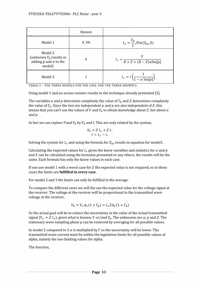
Known
Model 1 V, V0
Model 2 (unknown results in adding p and to the
model)
V
Model 3 I (
)
TABLE 2 – THE THREE MODELS FOR THE LINE, FOR THE THREE KNOWN’S.
Using model 1 and no access resistor results in the technique already presented [5].
The variables and determine completely the value of and determines completely the value of . Since the two are independent and are also independent of , this means that you can’t use the values of and to obtain knowledge about , but about and .
In fact we can replace and by and I. This are only related by the system,
Solving the system for and using the formula for results in equation for model1.
Calculating the expected values for given the know variables and statistics for and and can be calculated using the formulas presented or any others, the results will be the same. Each formula has only the know values in each case.
If one use model 1 with a worst case for the expected value is not required, so in these cases the limits are fulfilled in every case.
For model 2 and 3 the limits can only be fulfilled in the average.
To compare the different cases we will the use the expected value for the voltage signal at the receiver. The voltage at the receiver will be proportional to the transmitted wave voltage at the receiver,
So the actual goal will be to reduce the uncertainty in the value of the actual transmitted signal ( , given what is known, or/and . The unknowns are , and . The
stationary wave sampling phase p can be removed by averaging for all possible values.
In model 2 compared to 3 is multiplied by so the uncertainty will be lower. The transmitted wave current must be within the legislation limits for all possible values of alpha, namely the two limiting values for alpha.
The function,

PTDCEEA-TEL679792006 - PLC Noise - year 3
Page 14
[
]
is represented in Table 1. This can be used in the calculation. The results for the expected value for are in each model are,
Model
1
2
3
TABLE 3 – RESULTS FOR THE EXPECTED VALUE OF THE TRANSMITTED WAVE CURRENT.
Model 1 allows the removal of k that can be high.
In order to compare the techniques one should compare the actual value used for the signal with the maximum allowed one, if all the line characteristics were known.
For model 1 one has two similar equations, one defining the maximum value for given , namely,
And the other relating the value of given and .
Dividing both in order to eliminate results in,
As an example, let’s say , and results in,
The value of is chosen so that the current is bellow the maximum only in the average. For the case of model 2 one was, the minus is can be removed since is even,
Dividing once more results as before in,

PTDCEEA-TEL679792006 - PLC Noise - year 3
Page 15
As an example, let’s use the same values and , ( | |), (with the receiver very close let’s say ) the worst case for the reflection coefficient and (this is calculated using the worst case for , and ) . The value of would be . Results in,
Note that seems to indicate that this model (or technique) is better than one, but not that this will be within legislation limits only in the average, while technique one (or model) will work in every case. Instead of the expected value in we can also use the worst case for , this will result in | | . The result will be,
This will be worst than model 1, and there is still the problem that one can almost certain that will be greater than (about ) but not so certain that will be greater than .
For model 3 the result is (let’s call this the signal gap, ),
As an example using the values above and using the expected value results,
And for worst case,
A summary of the numerical results
Model Known
Assemble average Worst for
1 V, V0 --- 0.33
2 V 0.48 0.24
3 I 0.44 0.1
TABLE 4 – A SUMMARY OF THE NUMERICAL RESULTS FOR THE SIGNAL GAP.
Note that this are only example values, for instance the value for the line impedance is used in the EMC community but for the common mode and not the differential mode of the power lines. In telecommunications ports the value used is usually .
PTDCEEA-TEL679792006 - PLC Noise - year 3
Page 16
Note that if the assemble average was used the signal used in model 1 would be higher. If the maximum is limited then the average will be lower than the maximum, if we remove the maximum we can make the average equal to the maximum. In order to make this calculation we need to consider the correlation between and and . Note that and are the magnitude and phase of a virtual reflection coefficient at a virtual receiver, and so this is related to the line impedance.
The Signal Gap with a limit on the ensemble average was not calculated. This require knowledge of the joint probability density function of and , this should be independent for long lines, since the line length will randomize the value of , but this will not be true for short lines.
PTDCEEA-TEL679792006 - PLC Noise - year 3
Page 17
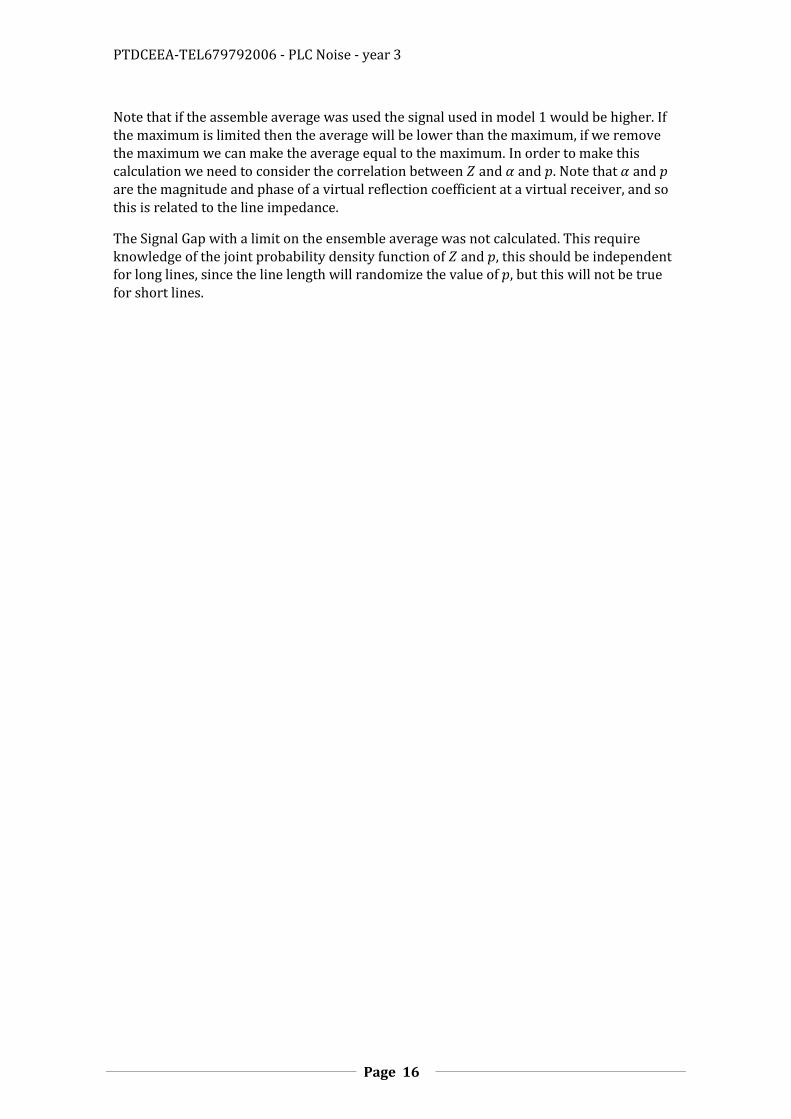
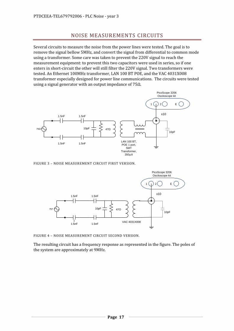
NOISE MEASUREMENTS CIRCUITS
Several circuits to measure the noise from the power lines were tested. The goal is to remove the signal bellow 5MHz, and convert the signal from differential to common mode using a transformer. Some care was taken to prevent the 220V signal to reach the measurement equipment: to prevent this two capacitors were used in series, so if one enters in short-circuit the other will still filter the 220V signal. Two transformers were tested. An Ethernet 100MHz transformer, LAN 100 BT POE, and the VAC 4031X008 transformer especially designed for power line communications. The circuits were tested using a signal generator with an output impedance of .
47Ω
1.5nF 1.5nF
1.5nF 1.5nF
LAN 100 BT,
POE 1 port,
SMT
Transformer,
350µH
75Ω 10pF
10pF
1 2 E
PicoScope 3206
Osciloscope kit
x10
FIGURE 3 – NOISE MEASUREMENT CIRCUIT FIRST VERSION.
47O
1.5nF 1.5nF
1.5nF 1.5nF
VAC 4031X008
75? 10pF
10pF
1 2 E
PicoScope 3206
Osciloscope kit
x10
FIGURE 4 – NOISE MEASUREMENT CIRCUIT SECOND VERSION.
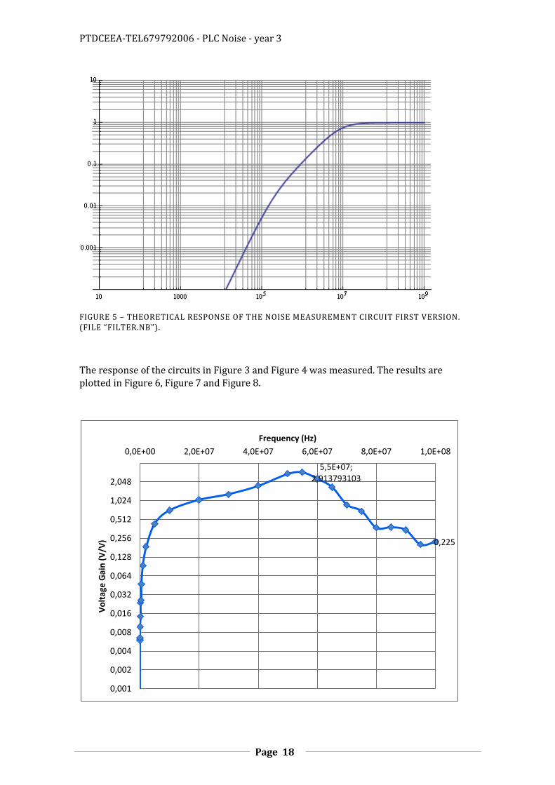
The resulting circuit has a frequency response as represented in the figure. The poles of the system are approximately at 9MHz.
PTDCEEA-TEL679792006 - PLC Noise - year 3
Page 18
FIGURE 5 – THEORETICAL RESPONSE OF THE NOISE MEASUREMENT CIRCUIT FIRST VERSION. (FILE “FILTER.NB”).
The response of the circuits in Figure 3 and Figure 4 was measured. The results are plotted in Figure 6, Figure 7 and Figure 8.
5,5E+07; 2,913793103
0,225
0,001
0,002
0,004
0,008
0,016
0,032
0,064
0,128
0,256
0,512
1,024
2,048
0,0E+00 2,0E+07 4,0E+07 6,0E+07 8,0E+07 1,0E+08
Vo
ltag
e G
ain
(V
/V)
Frequency (Hz)

PTDCEEA-TEL679792006 - PLC Noise - year 3
Page 19
FIGURE 6 – FREQUENCY RESPONSE OF THE CIRCUIT IN FIGURE 4 WITH A VAC TRANSFORMER.
FIGURE 7 – FREQUENCY RESPONSE OF THE CIRCUIT IN FIGURE 4 WITH A VAC TRANSFORMER IN LOG SCALE.
5,5E+07; 2,913793103
0,225
0,001
0,002
0,004
0,008
0,016
0,032
0,064
0,128
0,256
0,512
1,024
2,048
1,0E+02 8,0E+02 6,4E+03 5,1E+04 4,1E+05 3,3E+06 2,6E+07
Vo
ltag
e G
ain
(V
/V)
Frequency (Hz)

PTDCEEA-TEL679792006 - PLC Noise - year 3
Page 20
FIGURE 8 – FREQUENCY RESPONSE OF THE CIRCUIT IN FIGURE 3 WITH THE WE TRANSFORMER.
0,001
0,002
0,004
0,008
0,016
0,032
0,064
0,128
0,256
0,512
1,024
2,048
4,096
0,0E+00 2,0E+07 4,0E+07 6,0E+07 8,0E+07 1,0E+08
PTDCEEA-TEL679792006 - PLC Noise - year 3
Page 21
PARASITIC CAPACITORS AND INDUCTORS
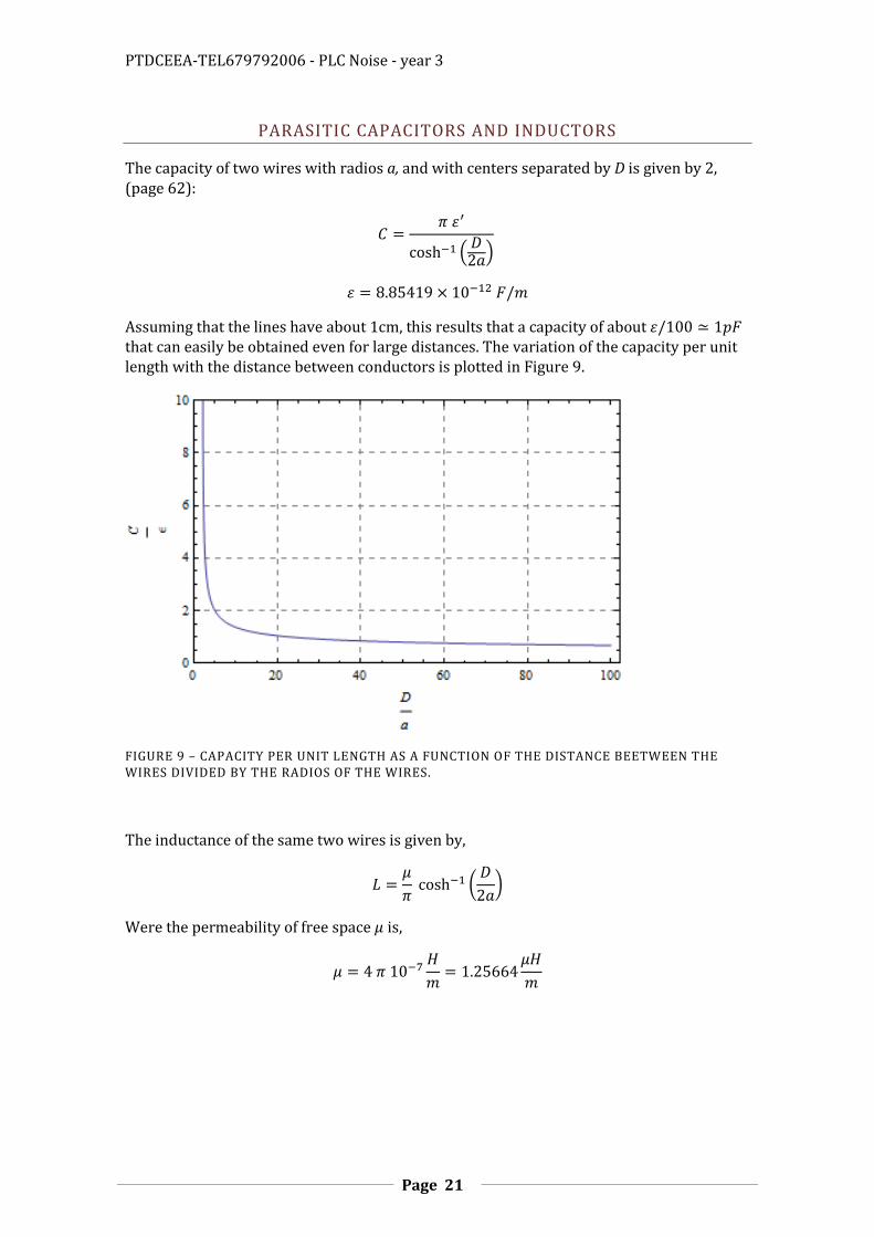
The capacity of two wires with radios a, and with centers separated by D is given by 2, (page 62):
(
)
Assuming that the lines have about 1cm, this results that a capacity of about that can easily be obtained even for large distances. The variation of the capacity per unit length with the distance between conductors is plotted in Figure 9.
FIGURE 9 – CAPACITY PER UNIT LENGTH AS A FUNCTION OF THE DISTANCE BEETWEEN THE WIRES DIVIDED BY THE RADIOS OF THE WIRES.
The inductance of the same two wires is given by,
(
)
Were the permeability of free space is,

PTDCEEA-TEL679792006 - PLC Noise - year 3
Page 22
FIGURE 10 – INDUCTANCE PER UNIT LENGTH AS A FUNCTION OF THE DISTANCE BETWEEN THE WIRES DIVIDED BY THE RADIOS OF THE WIRES.
The inductance of two lines with 1cm length 1mm radios and 5mm distance is, , and this results in an impedance of at 100MHz.
Note that for a given material the phase velocity is independent of the geometry, and this
is √ , so from this results that L and C are inversely proportional.
Oscilloscope probes:
These were designed to work with and osciloscopes.
In the 10x they have an input capacitance of and in the 1x mode +oscilloscope input capacitance.
For a source impedance of and the 10x probe the bandwidth is 318 MHz.
For a source impedance of and the 1x probe the bandwidth is 48 MHz.
The frequency response when the probe is compensated for a 20pF oscilloscope and the oscilloscope input is 18pF is as follows. At high frequencies’ the response of the probes is simple the ratio of the capacitors instead of the ration of the resistances, so the difference is not that great.

PTDCEEA-TEL679792006 - PLC Noise - year 3
Page 23
FIGURE 11 – FREQUENCY RESPONSE OF NOT SO COMPENSATED OSCILLOSCOPE PROBES.
A SMALL TRANSMISSION LINE
(
) (
) (
)
And
(
) (
) (
)
(
)
I0 I1
V0 V1
By assuming small values for one gets the following values for the parameters of the biport.
PTDCEEA-TEL679792006 - PLC Noise - year 3
Page 24
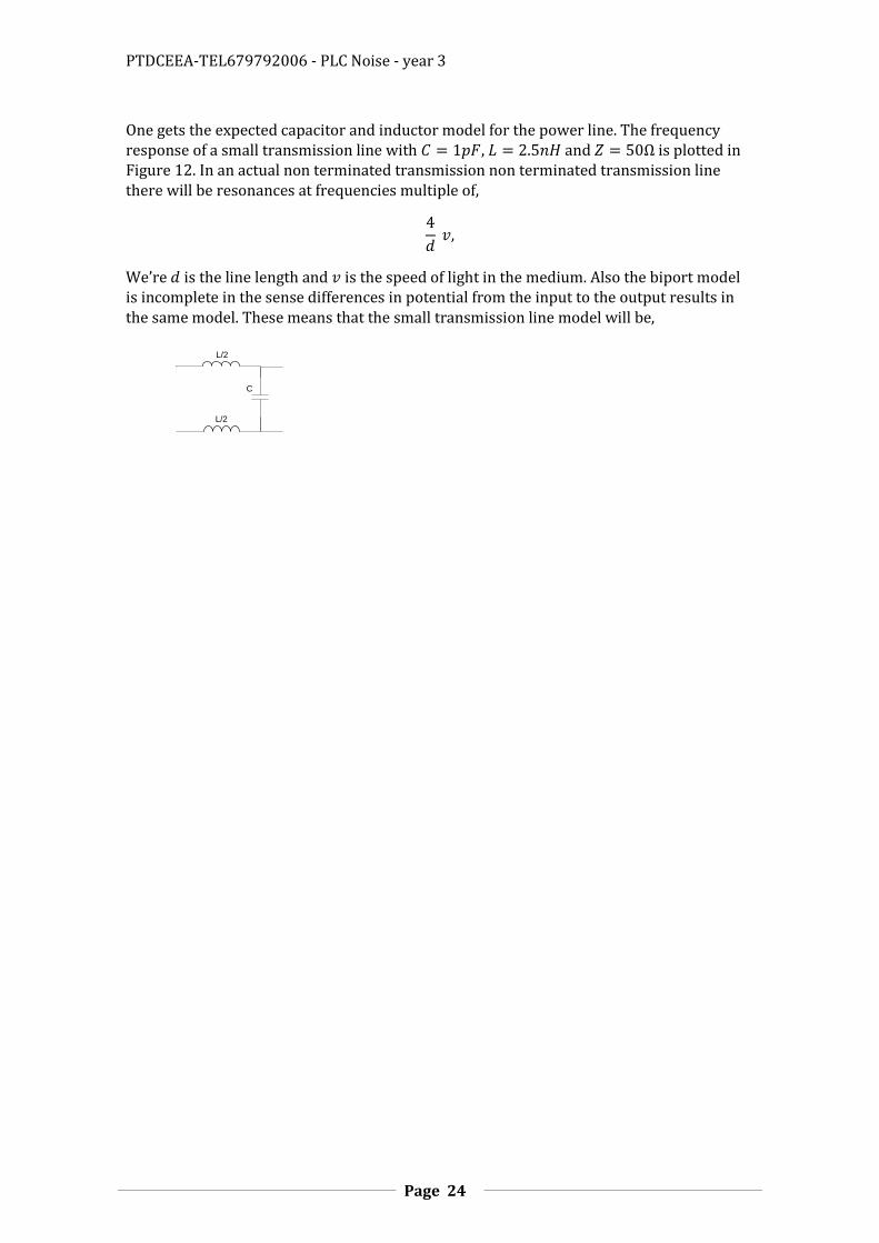
One gets the expected capacitor and inductor model for the power line. The frequency response of a small transmission line with , and is plotted in Figure 12. In an actual non terminated transmission non terminated transmission line there will be resonances at frequencies multiple of,
We’re is the line length and is the speed of light in the medium. Also the biport model is incomplete in the sense differences in potential from the input to the output results in the same model. These means that the small transmission line model will be,
L/2
L/2
C

PTDCEEA-TEL679792006 - PLC Noise - year 3
Page 25
FIGURE 12 – FREQUENCY RESPONSE OF A SMALL TRANSMISSION LINE WITH , AND . THE LINE HAS A LOW PASS CHARACTERISTIC. AN ACTUAL NON TERMINATED LINE WILL HAVE RESONANCES AND ZEROS AT CERTAIN FREQUENCIES.
The resonance frequency or the frequency of the first double poles of the line will be given by
√
√
This has a direct relation the value calculated using the phase velocity. The following discussion is for an open termination line with a low impedance source. The voltage of at a given point in the transmission line is the sum of the amplitudes of the positive and negative traveling waves. This means that is the traveled distance (two tines the length of the line) is half the wavelength then, when the reflected wave reaches the input it will cancel the voltage at that point: In order to maintain the voltage maintained by a low impedance source the positive wave will increase, causing after a delay an increase in the negative have and once more an increase in the positive wave, resulting in a resonance.
√
√
A capacitance at the termination of the line will lower the resonance frequency, because it will increase the phase of the voltage of the reflected wave. However, there is a factor of difference between the two models, but not that the small line approximation is no longer valid at the resonance frequency. This suggests a value for the frequency that a line can be used that it still functions as a more or less flat transfer function, without being properly terminated. This would be something like . The speed of light is independent of the geometry of the line, only depends on the materials. The value of for polyethylene, the most used plastic is 2.25. The resulting maximum frequency for a line with dimensions lower than is,
√
PTDCEEA-TEL679792006 - PLC Noise - year 3
Page 26
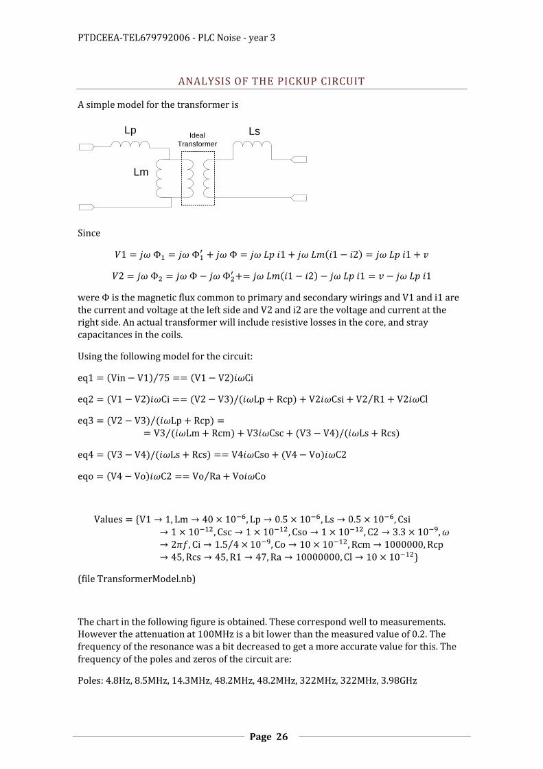
ANALYSIS OF THE PICKUP CIRCUIT
A simple model for the transformer is
Lp
Lm
LsIdeal
Transformer
Since
were is the magnetic flux common to primary and secondary wirings and V1 and i1 are the current and voltage at the left side and V2 and i2 are the voltage and current at the right side. An actual transformer will include resistive losses in the core, and stray capacitances in the coils.
Using the following model for the circuit:
⁄
⁄
⁄ ⁄
⁄
⁄
(file TransformerModel.nb)
The chart in the following figure is obtained. These correspond well to measurements. However the attenuation at 100MHz is a bit lower than the measured value of 0.2. The frequency of the resonance was a bit decreased to get a more accurate value for this. The frequency of the poles and zeros of the circuit are:
Poles: 4.8Hz, 8.5MHz, 14.3MHz, 48.2MHz, 48.2MHz, 322MHz, 322MHz, 3.98GHz

PTDCEEA-TEL679792006 - PLC Noise - year 3
Page 27
Zeros: 0Hz, 0Hz, 14.3MHz, 3.98GHz
The deviation from the ideal are mostly dictated by the filter formed by leakage primary and secondary inductance Lp, and Ls, the primary and secondary resistances due to losses in the transformer core, Rp and Rs, and the capacitance of the oscilloscope probes. These issues are further discussed in the following sections. There was also the possibility of a resonance between the primary inductance and the internal stray capacitance of the transformer. However, this would lead to higher values of the leakage inductance and the resonance with the oscilloscope capacitance would appear at lower frequencies, so this was ruled out.
FIGURE 13 – THEORETICAL RESPONSE CURVE FOR THE CIRCUIT.
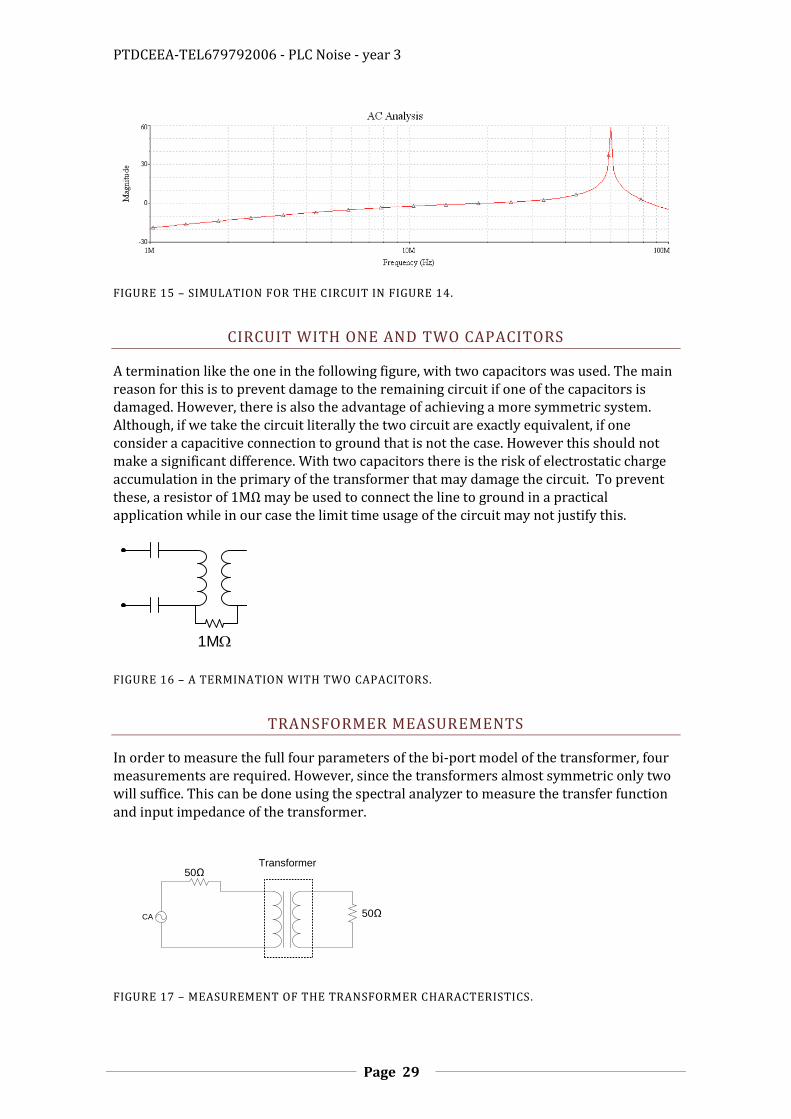
We also simulated a circuit similar to the one in Figure 4 as represented in Figure 14. The parameters were adjusted to obtain results similar to the measured values. The actual values of the parameters may be different however. The results of the simulation are presented in Figure 15. A resonance at 60MHz is easily seen corresponding to the resonance between L2 and C5, a parasitic capacitance of the transformer and the primary leakage inductance of the transformer. If a resistance of corresponding to losses in the core of the transformer were added in parallel with C5 then the peak in the response would be lower, and similar with measurements values. The same effect can be obtained by adding a charge resistance. Otherwise there are no losses resulting in a pure resonance.
We also made the simulation using Multisim, as presented below:
Schematic:

PTDCEEA-TEL679792006 - PLC Noise - year 3
Page 28
Simulation results:
And we made a simulation with a different circuit:
FIGURE 14 – SIMULATION FOR THE CIRCUIT IN FIGURE 4.
Rf
75Ω
Ci
375pFCsi1pF
R147Ω
Cl10pF
Rcp
45Ω
Lp
500nH
Lm40µH
Rcm1MΩ
Csc1pF
Rcs
45Ω
Ls
500nH
Cso1pF
C2
3.3nFRa10MΩ
Co10pF
V1
100mVrms
5MHz
0°
VIN V1 V2 V3 V4 V0
PTDCEEA-TEL679792006 - PLC Noise - year 3
Page 29
FIGURE 15 – SIMULATION FOR THE CIRCUIT IN FIGURE 14.
CIRCUIT WITH ONE AND TWO CAPACITORS
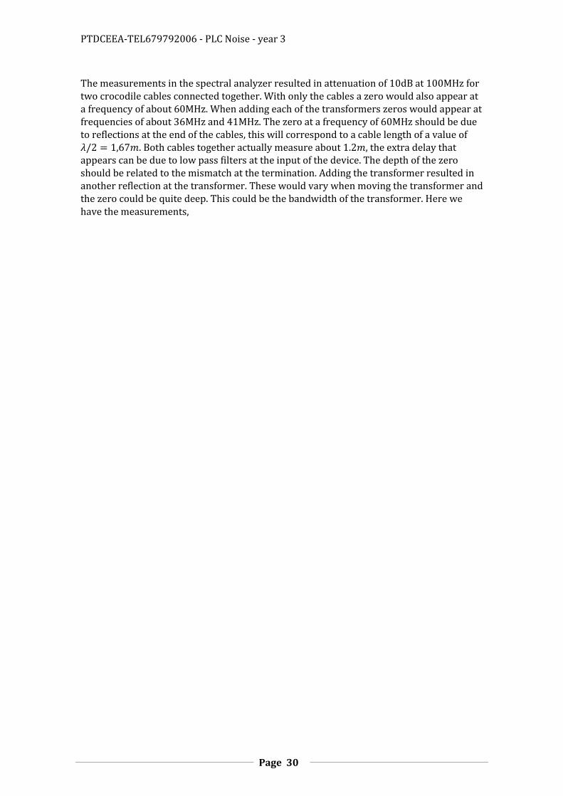
A termination like the one in the following figure, with two capacitors was used. The main reason for this is to prevent damage to the remaining circuit if one of the capacitors is damaged. However, there is also the advantage of achieving a more symmetric system. Although, if we take the circuit literally the two circuit are exactly equivalent, if one consider a capacitive connection to ground that is not the case. However this should not make a significant difference. With two capacitors there is the risk of electrostatic charge accumulation in the primary of the transformer that may damage the circuit. To prevent these, a resistor of may be used to connect the line to ground in a practical application while in our case the limit time usage of the circuit may not justify this.
1MW
FIGURE 16 – A TERMINATION WITH TWO CAPACITORS.
TRANSFORMER MEASUREMENTS
In order to measure the full four parameters of the bi-port model of the transformer, four measurements are required. However, since the transformers almost symmetric only two will suffice. This can be done using the spectral analyzer to measure the transfer function and input impedance of the transformer.
Transformer50Ω
CA 50Ω
FIGURE 17 – MEASUREMENT OF THE TRANSFORMER CHARACTERISTICS.
PTDCEEA-TEL679792006 - PLC Noise - year 3
Page 30
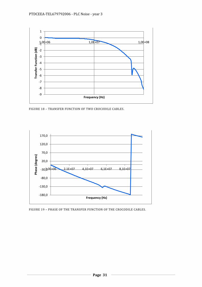
The measurements in the spectral analyzer resulted in attenuation of at 100MHz for two crocodile cables connected together. With only the cables a zero would also appear at a frequency of about 60MHz. When adding each of the transformers zeros would appear at frequencies of about 36MHz and 41MHz. The zero at a frequency of 60MHz should be due to reflections at the end of the cables, this will correspond to a cable length of a value of . Both cables together actually measure about , the extra delay that appears can be due to low pass filters at the input of the device. The depth of the zero should be related to the mismatch at the termination. Adding the transformer resulted in another reflection at the transformer. These would vary when moving the transformer and the zero could be quite deep. This could be the bandwidth of the transformer. Here we have the measurements,
PTDCEEA-TEL679792006 - PLC Noise - year 3
Page 31
FIGURE 18 – TRANSFER FUNCTION OF TWO CROCODILE CABLES.
FIGURE 19 – PHASE OF THE TRANSFER FUNCTION OF THE CROCODILE CABLES.
-9
-8
-7
-6
-5
-4
-3
-2
-1
0
1
1,0E+06 1,0E+07 1,0E+08
Tran
sfe
r Fu
nct
ion
(d
B)
Frequency (Hz)
-180,0
-130,0
-80,0
-30,0
20,0
70,0
120,0
170,0
1,0E+06 2,1E+07 4,1E+07 6,1E+07 8,1E+07
Ph
ase
(d
egr
es)
Frequency (Hz)

PTDCEEA-TEL679792006 - PLC Noise - year 3
Page 32
FIGURE 20 – TRANSFER FUNCTION OF THE MEASUREMENT WITH A VAC TRANSFORMER.
FIGURE 21 – PHASE OF THE TRANSFER FUNCTION OF THE VAC TRANSFORMER.
-10
-9
-8
-7
-6
-5
-4
-3
-2
-1
0
1,0E+06 1,0E+07 1,0E+08Tr
ansf
er
fun
ctio
n (
dB
)
Frequency (Hz)
-180,0
-130,0
-80,0
-30,0
20,0
70,0
120,0
170,0
1,0E+06 1,0E+07 1,0E+08
Ph
ase
(d
egr
ee
s)
Frequency (Hz)

PTDCEEA-TEL679792006 - PLC Noise - year 3
Page 33
FIGURE 22 – TRANSFER FUNCTION WITH A COILCRAFT TRANSFORMER.
FIGURE 23 – PHASE OF THE TRANSFER FUNCTION OF THE COILCRAFT TRANSFORMER.
-12,0
-10,0
-8,0
-6,0
-4,0
-2,0
0,0
1,0E+06 1,0E+07 1,0E+08Tr
ansf
er
Fun
ctio
n (
dB
)
Frequency (Hz)
-180,0
-130,0
-80,0
-30,0
20,0
70,0
120,0
170,0
1,0E+06 1,0E+07 1,0E+08
Ph
ase
(d
egr
ee
s)
Frequency (Hz)

PTDCEEA-TEL679792006 - PLC Noise - year 3
Page 34
We made the following simulation of the measurement setup.
Schematic:
The parameters were,
Inductance: 2.50836e-007 H
Capacitance: 1.00334e-010 F
Simulation results:
W2
0.5 m 0 Ω
W1
0.7 m 0 Ω
R260Ω
OUTPUT
V1
120 Vrms
60 Hz
0°
R3
50Ω
VIN
R110Ω

PTDCEEA-TEL679792006 - PLC Noise - year 3
Page 35
The following is a simulation of the measurements, using two crocodile cables modeled as transmission lines and a model for the VAC transformer.
Schematic:
Transmission line parameters
Line 1:
Length of the transmission line: 500 mm
Resistance per unit length: 0 Ohm
Inductance per unit length: 2.50836e-007 H
Capacitance per unit length: 1.00334e-010 F
Line 2:
Length of the transmission line: 700 mm
Resistance per unit length: 0 Ohm
Inductance per unit length: 2.50836e-007 H
Capacitance per unit length: 1.00334e-010 F
Simulation results:
Rf
50Ω
Csi0.1pF
Rcp
45Ω
Lp
500nH
Lm40µH
Rcm1MΩ
Csc0.1pF
Rcs
45Ω
Ls
500nH
Cso0.1pF
V1
100mVrms
5MHz
0°
VIN
V3
W1
500mm 0 Ω
W2
700mm 0 Ω
V1
R250Ω
Vo
V4V2
PTDCEEA-TEL679792006 - PLC Noise - year 3
Page 36
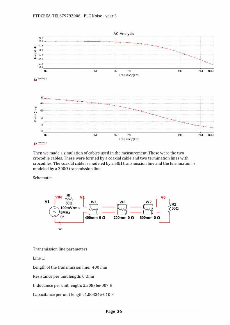
Then we made a simulation of cables used in the measurement. These were the two crocodile cables. These were formed by a coaxial cable and two termination lines with crocodiles. The coaxial cable is modeled by a transmission line and the termination is modeled by a transmission line.
Schematic:
Transmission line parameters
Line 1:
Length of the transmission line: 400 mm
Resistance per unit length: 0 Ohm
Inductance per unit length: 2.50836e-007 H
Capacitance per unit length: 1.00334e-010 F
Rf
50ΩV1
100mVrms
5MHz
0°
VIN
W1
400mm 0 Ω
W2
600mm 0 Ω
V1
R250Ω
V0
W3
200mm 0 Ω

PTDCEEA-TEL679792006 - PLC Noise - year 3
Page 37
Line 2:
Length of the transmission line: 200 mm
Resistance per unit length: 0 Ohm
Inductance per unit length: 1.50502e-006H
Capacitance per unit length: 1.67224e-011F
Line 3:
Length of the transmission line: 600 mm
Resistance per unit length: 0 Ohm
Inductance per unit length: 2.50836e-007 H
Capacitance per unit length: 1.00334e-010 F
Simulation results:
There is a resonance in the middle line that at the frequency were . Note that when the charge impedance is lower that the line impedance the signal of the amplitude of the wave inverts. At half this distance the reflection subtract resulting in a valley. This is what is shown in the simulation, and in agreement with the measurements.
PTDCEEA-TEL679792006 - PLC Noise - year 3
Page 38
ANALYZING THE MEASUREMENTS OF THE COILCRAFT WB1-1
The Coilcraft transformer should have a to bandwidth; however a null at about was measured suggesting that this is the concentrated parameter bandwidth. Some questions may be raised to if the transformer should be used as transmission line transformer, in lay down configuration. However, looking at the figure of its typical response bellow shows that this is not the case, since transmission line transformers pass the differential signal all the way to DC. In fact the high pass characteristic is consistent with the input impedance, since this for results in 3dB cut off frequency of . The series resistance consistent with 0.5dB attenuation in the pass band should be .
FIGURE 24 – TYPICAL RESPONSE OF THE COILCRAFT WB1-1 TRANSFORMER.
For a transformer to have impedance (which is typical) and a zero at the values for L and C should be, and . It the bandwidth is determined by the leakage inductance and the charge resistance then the same value is obtained for . If the zero is at as measured then capacitor should be about
which is too high.
The crocodile cables can have an inductance much greater than the leakage inductance. For 1mm wires at a distance of 2dm the parameters of the line are, and , resulting in an impedance of .
50Ω
CA
50Ω
2.1uH
2.1uH
2.1uH
2.1uH
27x2uH 27x2uH
15.9/2nH 15.9/2nH
6.37/3pF
6.37/3pF
6.37/3pF
FIGURE 25 – MODEL FOR THE MEASUREMENTS WITH THE COILCRAFT TRANSFORMER.
In this circuit the wire inductance will appear in parallel with the

PTDCEEA-TEL679792006 - PLC Noise - year 3
Page 39
PTDCEEA-TEL679792006 - PLC Noise - year 3
Page 40
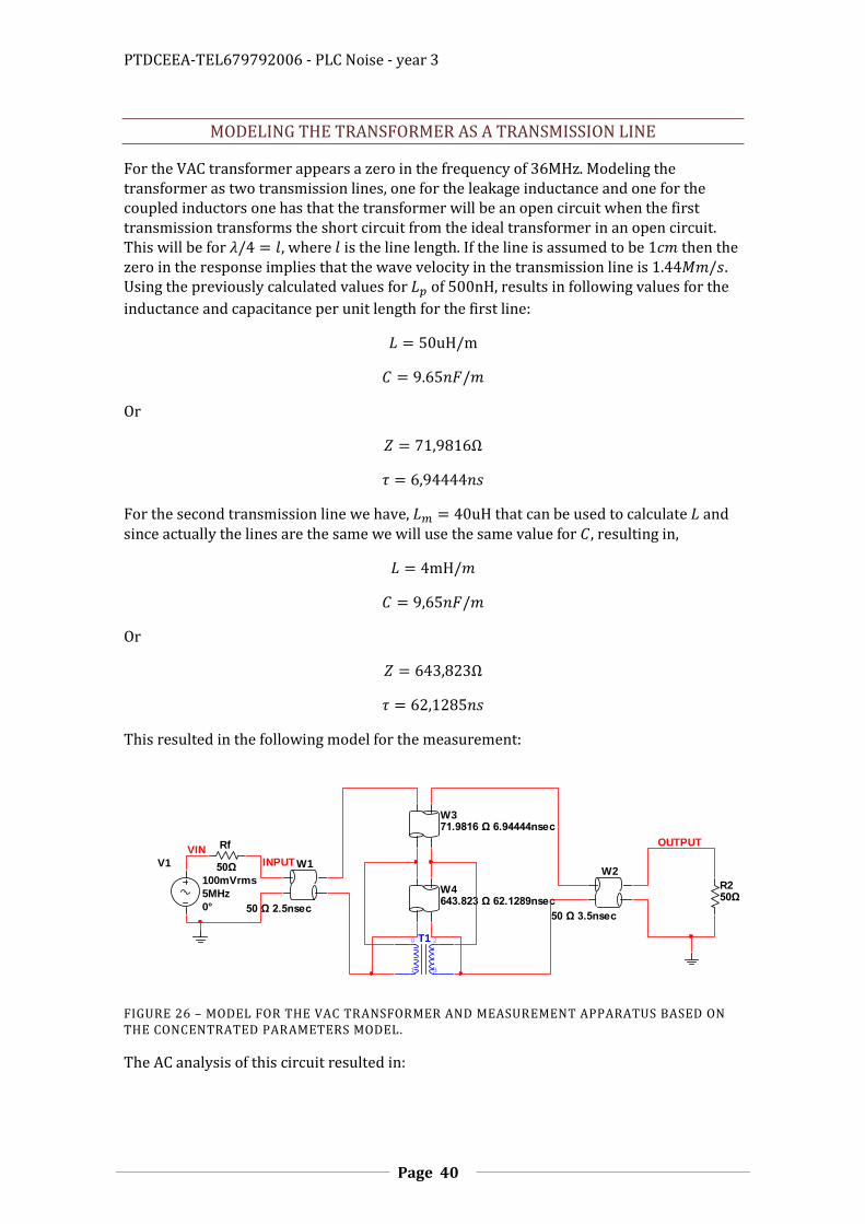
MODELING THE TRANSFORMER AS A TRANSMISSION LINE
For the VAC transformer appears a zero in the frequency of . Modeling the transformer as two transmission lines, one for the leakage inductance and one for the coupled inductors one has that the transformer will be an open circuit when the first transmission transforms the short circuit from the ideal transformer in an open circuit. This will be for , where is the line length. If the line is assumed to be then the zero in the response implies that the wave velocity in the transmission line is . Using the previously calculated values for of , results in following values for the
inductance and capacitance per unit length for the first line:
Or
For the second transmission line we have, that can be used to calculate and since actually the lines are the same we will use the same value for , resulting in,
Or
This resulted in the following model for the measurement:
FIGURE 26 – MODEL FOR THE VAC TRANSFORMER AND MEASUREMENT APPARATUS BASED ON THE CONCENTRATED PARAMETERS MODEL.
The AC analysis of this circuit resulted in:
Rf
50ΩV1
100mVrms
5MHz
0°
VIN
R250Ω
T10
1
2
3
W4643.823 Ω 62.1289nsec
W371.9816 Ω 6.94444nsec
W1
50 Ω 2.5nsec
INPUTW2
50 Ω 3.5nsec
OUTPUT

PTDCEEA-TEL679792006 - PLC Noise - year 3
Page 41
FIGURE 27 – AC ANALYSIS OF THE CIRCUIT IN THE FIGURE.
The zeros are not in the same frequency of the zeros of the transformer so some more work needs to be done. Actually this analysis would be correct if both ends of the transformer were connected to ground as in the following circuit.
Simulations Results:
Rf1
50ΩV1
100mVrms
5MHz
0°
R250Ω
W371.9816 Ω 6.94444nsec
W1
50 Ω 2.5nsec
W2
50 Ω 3.5nsec
W4643.823 Ω 62.1289nsec
T10
1
2
3
Vo1V1VIN
V2 Vo2

PTDCEEA-TEL679792006 - PLC Noise - year 3
Page 42
In order to obtain a result similar to the measurements, we changed the capacitance per unit length of the lines to,
This resulted in the following circuit,
And the following simulations results that are closer to the measurements,
Rf
50ΩV1
100mVrms
5MHz
0°
VIN
R250Ω
W1
50 Ω 2.5nsec
V1
W2
50 Ω 3.5nsec
Vo
T10
1
2
3
W3227.626 Ω 2.19659nsec
W42035.95 Ω 19.6469nsec

PTDCEEA-TEL679792006 - PLC Noise - year 3
Page 43
COMMON AND DIFFERENTIAL MODE TRANSMISSION LINE TRANSFORMER
This model was based on the concentrated parameters model. A more accurate model of the transformer is can be obtained if by considering o transmission line model for differential and common mode propagation. A distributed transformer should be modeled by a series of infinitesimally small transformers as in the following figure,
…..Lf LM
CCM
2CD
2CD
Lf
Lf LM
CCM
2CD
2CD
Lf
FIGURE 28 – A TRANSMISSION LINE MODEL FOR A TRANSFORMER.
This represents a three wire transmission line, and results in propagation in two modes, differential and common model. In differential mode propagation the effect of the transformer, corresponding to the two inductors with inductance , will cancel out, resulting that the characteristic parameters of the line will be and . For
the common mode propagation the parameters of the line will be and
. All this are units per unit length. Actually this should be the model for any realistic transmission line. The third line can be ground or earth, and it is assumed that is doesn’t have any inductance.
Common mode and differential mode signals are and and and , resulting that and . The following two circuits are equivalent. In some cases the superposition theorem can be used to analyze circuits in terms of common mode and differential mode,
R1
VA
R2
VB
R1
VCM
R2
VD/2
-VD/2
FIGURE 29 – COMMON MODE AND DIFFERENTIAL MODE.

PTDCEEA-TEL679792006 - PLC Noise - year 3
Page 44
In power line communications we would like to filter out the common mode and leave only the differential mode, since differential mode radiation is much lower and common mode noise is much higher.
Filtering out the common mode can be done by connecting it to ground, while keeping the differential mode terminated, in something like,
R/2
R/2
FIGURE 30 – CONNECTING THE COMMON MODE TO GROUND.
This wouldn’t even require a transformer, just two resistors and two capacitors to ground. The signal could be measured in one of the lines. However, the signal will be halved and it will fail if the signal source is not purely differential. Also, any common mode signal would appear as additional noise. The signal can then be measured in any of the lines. Also, it will produce common mode currents that will radiate.
A better option should be to leave the common mode open. This is the effect produced by the transformer. If the circuit above is followed by a transformer, then the common mode will be connected to ground through the magnetization inductance of the transformer that should function as an open circuit. This will eliminate the common mode current. This is represented in the following circuit,
R/2
R/2
Out
FIGURE 31 – HIGH COMMON MODE INPUT IMPEDANCE WITH A TRANSMISSION LINE TRANSFORMER.
In this circuit high common mode impedance will filter the common mode signal. Since this will not be always high, the common mode noise will not always be filtered. Typical values for inductor resonances can be since wave velocity can be very low in an inductor.
The most obvious similar circuit with a single resistor to ground is similar, but will create a differential mode to common mode conversion at high frequencies, since common mode will be connected to and not ground. This should not be a big problem since at these frequencies the differential mode signal will mostly be noise.
Another, option is to terminate the common mode. This must be done by a large resistor, and this means that a large capacitors would be required to filter the , common mode signal.
A possible circuit to terminate the common mode and differential mode would be:

PTDCEEA-TEL679792006 - PLC Noise - year 3
Page 45
Rd/2
Rd/2 Rcm-Rd/4
FIGURE 32 – TERMINATING THE COMMON MODE (WILL RESULT IN COMMON MODE NOISE).
The common mode noise could be removed by a differential amplifier and long as the common mode signal is removed by the capacitors and the common mode resistance to ground. The capacitors should not be too large so that they can cut low frequencies, even with a large common mode resistance.
Rd/2
Rd/2 Rcm-Rd/4
+-
In1
In2
Out
FIGURE 33 – A CIRCUIT FOR MEASUREMENT OF THE DIFFERENTIAL SIGNAL IN PLC SIGNAL WITHOUT A TRANSFORMER.
A transformer can also be added to increase common mode input resistance. The value of common termination resistor could be lowered to make it easier to filter the , although oscillations on the common mode termination resistance of the hole circuit would appear.
If the is small adding a transformer will have high common mode input resistance al lower frequencies. This is where it matters most, since at higher frequencies there will be other connections of the common mode to ground through the line resulting in multiple reflections. Adding a differential amplifier allows to filter common mode noise to very high frequencies.
TRADITIONAL BALAUNS CIRCUITS
Transformer circuits that can be used to convert from balanced to unbalanced signals. These circuits however do not terminate transmission line transformers so they may not work at very high frequencies. Their functions can also be achieved using electronic amplifiers.
AC
FIGURE 34 – UNBALENCED TO BALANCED CONVERTER (A DRIVE CIRCUIT).

PTDCEEA-TEL679792006 - PLC Noise - year 3
Page 46
In1
In2
R
Out
FIGURE 35 – BALANCED TO UNBALENCED CONVERTER (A RECEIVER CIRCUIT).
INDUCTORS
To be checked.
A typical inductor should be modeled by the following circuit, with infinitesimal elements,
…..C
L
Cx
C
L
Cx
FIGURE 36 – MODEL FOR AN INDUCTOR.
Since and are infinitesimal its resonance frequency will be very high, and at typical applications the component should dominate, so the inductor will have no parallel capacitance due to inter coil capacitance, but just a capacitor to earth.
Note that at self resonance the inductor impedance starts to decrease, but it is still high for a while.
The capacitance between a two single coils should be of the order of
.
This value was calculated for two lines at a space of equal to 4 times their radios and a length of . The equivalent capacity in parallel with the inductor will be equal to this divided by the number of coils.
A simplified formula for the calculation of the inductance of an inductor is
⁄
This results that for an inductor with
The inductance will be
This will result in a resonance due to the parallel capacitors at
√ MHz

PTDCEEA-TEL679792006 - PLC Noise - year 3
Page 47
The resonance due to the capacitance to earth should also be at high frequencies. A formula for the calculation of the self capacitance of an inductor is, 3
(
√ )
COILCRAFT WIDEBAND TRANSFORMER DISTORTION MEASUREMENTS
Harmonic Distortion of the Coilcraft Wideband Transformer
Signal: 15MHz, -40dBm
Harmonics Amplitude (dBm)
15MHz -40.9541
30MHz under -80.9996
Signal: 15MHz, 1dBm
Harmonics Amplitude (dBm)
15MHz 0.340732
30MHz -48.5842
45MHz -64.2304
Signal: 50MHz, 1dBm
Harmonics Amplitude (dBm)
50MHz -5.49019
100MHz -57.3783
150MHz -67.6661
AMPLIFIER
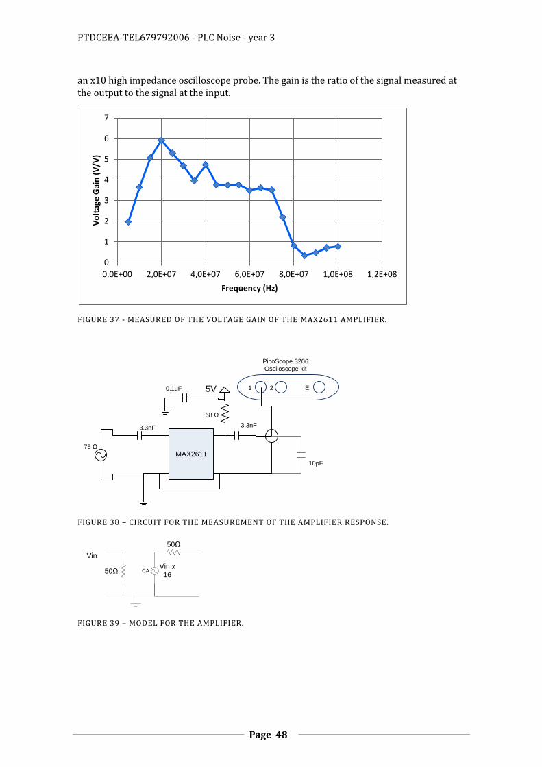
IC AMPLIFIER MEASUREMENTS
The voltage gain of the RF amplifier MAX2611 was measured. The results of the measurements are plotted in Erro! A origem da referência não foi encontrada.. This was measured by connecting the input of the amplifier to the signal generator through a coaxial cable with alligators and measuring the signal at the input and at the output using
PTDCEEA-TEL679792006 - PLC Noise - year 3
Page 48
an x10 high impedance oscilloscope probe. The gain is the ratio of the signal measured at the output to the signal at the input.
FIGURE 37 - MEASURED OF THE VOLTAGE GAIN OF THE MAX2611 AMPLIFIER.
MAX2611
1 2 E
PicoScope 3206
Osciloscope kit
5V
3.3nF
68 Ω
0.1uF
75 Ω
3.3nF
10pF
FIGURE 38 – CIRCUIT FOR THE MEASUREMENT OF THE AMPLIFIER RESPONSE.
CA
50Ω
50Ω
Vin
Vin x
16
FIGURE 39 – MODEL FOR THE AMPLIFIER.
0
1
2
3
4
5
6
7
0,0E+00 2,0E+07 4,0E+07 6,0E+07 8,0E+07 1,0E+08 1,2E+08
Vo
ltag
e G
ain
(V
/V)
Frequency (Hz)

PTDCEEA-TEL679792006 - PLC Noise - year 3
Page 49
FIGURE 40 – THEORETICAL CIRCUIT FOR THE MEASUREMENTS OF THE IC AMPLIFIER RESPONSE.
FIGURE 41 – FREQUENCY RESPONSE OF THE CIRCUIT IN FIGURE 40.
Trying to refine the model resulted in,
FIGURE 42 – A SECOND MODEL FOR THE CIRCUIT.
V1
120 Vrms
60 Hz
0°
L1
30nH
L2
30nH
C1
3.3nF
C23pF
R150Ω
R2
50Ω
L3
30nH
C33pF
C4
3.3nF
C53pF
C710pF
C83pF
R3
68Ω
C9
100nF
L4
3nH
L5100nH
V2
5 V
V316 V/V
VIN L6
30nH
OUTPUT
V1
120 Vrms
60 Hz
0°
L1
15nH
L2
15nH
C1
3.3nF
C23pF
R150Ω
R2
50Ω
L3
15nH
C33pF
C4
3.3nF
C53pF
C710pF
C83pF
R3
68Ω
C9
100nF
L4
3nH
L5100nH
V2
5 V
V316 V/V
L6
15nH
L7
15nH
L8
15nH
L930nH
L10
15nHL11
15nH
VIN
C6
400fF
C10
100fF
C11
100fF L12
15nH
L13
15nH
OUTPUT

PTDCEEA-TEL679792006 - PLC Noise - year 3
Page 50
But the simulation results is very similar,
FIGURE 43 – AND ALMOST THE SAME RESULT.
And they do not agree with the measurements.
The inductance of a 3cm length wire 0.2mm diameter is the used for the inductors (http://www.consultrsr.com/resources/eis/induct5.htm). This is distributed over the upper and lower coils of the transmission line. However, the formula above calculates the inductance of two wires is more accurate than the calculation using the total flux.
The S-parameters of the network relate the amplitude of incident and reflected waves. Namely, we have
*
+ [
] *
+
The “a” parameters represent waves that flow into the circuit and the “b” parameters waves that flow out of the circuit.
And
a1
b1
a2
b2
FIGURE 44 – VARIABLES USED IN THE S PARAMETERS.
The S-parameters of the amplifier at 100MHz are:
S11 is the input reflection: S12 is the reverse gain: S21 is gain: S22 if the output reflection:
So the amplifier has well defined input and output impedances of and an inverting gain of 8.9.
TYPICAL IC AMPLIFIER
The internal circuit for the IC amplifiers used in the project is,

PTDCEEA-TEL679792006 - PLC Noise - year 3
Page 51
FIGURE 45 - TYPICAL CIRCUIT FOR AN IC AMPLIFIER.
The charge will be a resistance. In a typical application the amplifier will have a high impedance current output and must be loaded with a charge. The polarization is done with a resisted and an inductor. If the polarization is done with a resistance, then the output resistance will be , matched to the channel but the gain will be half.
An example for the values for the resisters are, , , . For an ideal transistor this will result in a input resistance an open loop gain of 10 a DC output of and current of for a power supply. The actual gain would be lower due to feedback through the R2 resister, so the values need some adjustment.

PTDCEEA-TEL679792006 - PLC Noise - year 3
Page 52
MEASUREMENTS CIRCUIT WITH AN IC AMPLIFIER
An amplifier was added at the circuit output. The resulting circuit is:
47Ω
1.5nF 1.5nF
1.5nF 1.5nF
VAC 4031X008
75Ω 16x1pF
1 2 E
PicoScope 3206
Osciloscope kit
5V
47Ω
3.3nF
68Ω
0.1uF
3.3nF
10pF
Lp=Ls=4uH
Lm=40uH
FIGURE 46 – NOISE MEASUREMENT CIRCUIT THIRD VERSION.
CA
50Ω
50Ω
Vin
Vin x
16
FIGURE 47 – MODEL FOR THE AMPLIFIER.
In the following version the input capacitors were exchanged by a capacitor as indicated by the transformer manufacture. Also the output resistance was removed since the amplifier already has a termination resistance to Vcc. The output was open for DC vales resulting in low frequency noise at the oscilloscope, but this was not a concern when measuring the circuit response.
10nF
VAC 4031X008
75Ω 16x1pF
1 2 E
PicoScope 3206
Osciloscope kit
5V
68Ω
0.1uF
3.3nF
10pF
Lp=Ls=4uH
Lm=40uH 3.3nF
FIGURE 48 – NOISE MEASUREMENT CIRCUIT 4TH VERSION.

PTDCEEA-TEL679792006 - PLC Noise - year 3
Page 53
Figure 49 – Voltage gain of the circuit in Figure 48.
There is something wrong with these measurements. There would be too much losses in the transformer do to the leakage inductance, for one to get such a result. At 100MHz a inductor of has an impedance of .
1,0
2,0
4,0
8,0
16,0
0,0E+00 2,0E+07 4,0E+07 6,0E+07 8,0E+07 1,0E+08
Vo
ltag
e G
ain
(V
/V)
Frequency (Hz)

PTDCEEA-TEL679792006 - PLC Noise - year 3
Page 54
By measuring the signal at the output of the transformer and at the output of the full circuit, the gain of the amplifier can be calculated. This is plotted in the following figure.
FIGURE 50 – VOLTAGE GAIN OF THE AMPLIFIER INSERTED IN THE CIRCUIT OF FIGURE 48.
20nF
VAC 4031X008
75Ω MAX26111pF
1 2 E
PicoScope 3206
Osciloscope kit
5V
68Ω
0.1uF
3.3nF
(46+20)pF
Lp=Ls=4uH
Lm=40uH
20nF
X1 probe
FIGURE 51 – NOISE MEASUREMENT CIRCUIT 5TH VERSION.
1,0
2,0
4,0
8,0
16,0
32,0
0,0E+00 2,0E+07 4,0E+07 6,0E+07 8,0E+07 1,0E+08
Vo
ltag
e G
ain
(V
/V)
Frequency (Hz)

PTDCEEA-TEL679792006 - PLC Noise - year 3
Page 55
AMPLIFIER DISTORTION
In order to use the 8bits of the data storage oscilloscope, one needs to have an error bellow 1/256/2=1/512 at the output of the amplifier. Most RF amplifiers specify the output power at 1dB compression of the output. A 1dB compression corresponds to the point where the output power is decreased by 1dB, and this corresponds roughly to a decrease in 12% in the signal amplitude. This is not the same but should not be too far from the point in the static voltage input output chart is 12% bellow from the strait line that would correspond to a linear amplifier.
For a simpler amplifier formed by a single transistor in common emitter configuration with a gain of 49.5dB (300) and a collector resistor of the input output relation is as represented in the Figure 52.
FIGURE 52 – INPUT OUTPUT RELATION OF A TYPICAL AMPLIFIER.
One can calculate the compression as a function of the input signal for an amplifier polarized to with an input voltage of corresponding to a mid scale output of . This is represented in Figure 53. The curve is similar to a hyperbola, and in fact this is what would be obtained if the second derivative of the transfer curve is assumed to be constant. This in turn can be used to derive the new limit of the signal. One has
And
Resulting in

PTDCEEA-TEL679792006 - PLC Noise - year 3
Page 56
FIGURE 53 – COMPRESSION IN THE INPUT OUTPUT RELATION OF AN AMPLIFIER.
IP3 POINT
The IP3 is the value of the output power for a theoretical point were power of the third order component of the amplifier gain is equal to the linear signal power. It is assumed that the amplifier gain can be expressed in a Taylor series, and since the amplifier should be more or less symmetric around the operation point, the second order term is small and the third order term dominates. The third order term power rises by 3dB for each increase of the input power by one dB, so at a given point the power of the two signals will become equal. The third order term represents amplifier distortion noise. The signal to distortion noise ratio at a given input level can then be estimated by,
Were is the output signal level, and is the IP3 point.
For the ZFL-500 amplifier the IP3 point is 18dBm. The quantization noise of an n-bits AD converter is given by,
While the signal is
So the signal to noise is
In order to have the distortion signal bellow the quantization noise one has to have,
PTDCEEA-TEL679792006 - PLC Noise - year 3
Page 57
Resulting in , that corresponds to . Comparing with the results from the previous section, one has that the ZFL-500 has a 1dB compression point of 9dBm, corresponding to , and the limit would be , so the results are not very different. This means that if the signal is below the minimum scale of of the PicoScope, the distortion should be lower than the quantization noise of the oscilloscope.
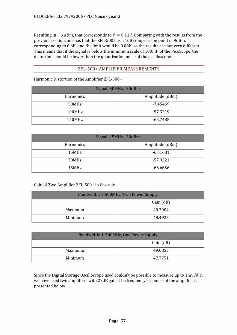
ZFL-500+ AMPLIFIER MEASUREMENTS
Harmonic Distortion of the Amplifier ZFL-500+
Signal: 50MHz, -30dBm
Harmonics Amplitude (dBm)
50MHz -7.45469
100MHz -57.3219
150MHz -65.7485
Signal: 15MHz, -30dBm
Harmonics Amplitude (dBm)
15MHz -6.01681
30MHz -57.9221
45MHz -65.6656
Gain of Two Amplifier ZFL-500+ in Cascade
Bandwidth: 1-500MHz, Two Power Supply
Gain (dB)
Maximum 49.3904
Minimum 48.4925
Bandwidth: 1-500MHz, One Power Supply
Gain (dB)
Maximum 49.0853
Minimum 47.7751
Since the Digital Storage Oscilloscope used couldn’t be possible to measure up to 1mV/div, we have used two amplifiers with 22dB gain. The frequency response of the amplifier is presented below:
PTDCEEA-TEL679792006 - PLC Noise - year 3
Page 58
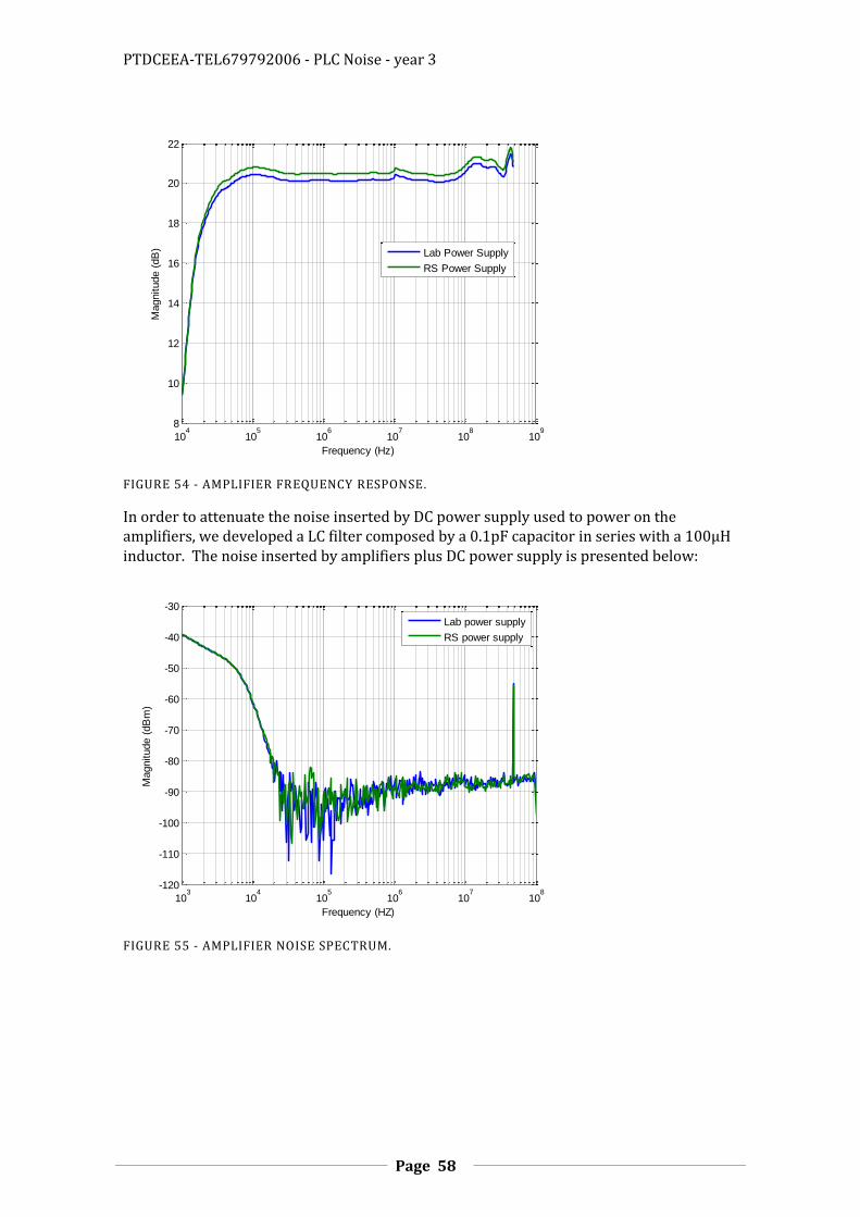
FIGURE 54 - AMPLIFIER FREQUENCY RESPONSE.
In order to attenuate the noise inserted by DC power supply used to power on the amplifiers, we developed a LC filter composed by a 0.1pF capacitor in series with a 100µH inductor. The noise inserted by amplifiers plus DC power supply is presented below:
FIGURE 55 - AMPLIFIER NOISE SPECTRUM.
104
105
106
107
108
109
8
10
12
14
16
18
20
22
Frequency (Hz)
Magnitude (
dB
)
Frequency Response Amplifier with Lab Power Supply vs RS Power Supply
Lab Power Supply
RS Power Supply
103
104
105
106
107
108
-120
-110
-100
-90
-80
-70
-60
-50
-40
-30
Frequency (HZ)
Magnitude (
dB
m)
Noise Measurement with RS/Lab Power Supply and Filter
Lab power supply
RS power supply

PTDCEEA-TEL679792006 - PLC Noise - year 3
Page 59
ZFL-500LN+ AMPLIFIER MEASUREMENTS
We also made the measurements with a new set of amplifiers that are similar to previous ones. These are the Mini-Circuits ZFL-500LN+ low noise amplifier (LN). The frequency response is presented below.
FIGURE 56 – ZFL-500LN+ FREQUENCY RESPONSE.
AMPLIFIER NOISE FIGURE
The noise figure of an amplifier is the ratio (in dB) of the equivalent voltage noise source at the input of the amplifier to the thermal noise of a resistor that is matched to amplifier impedance. The thermal noise of a resistor is,
√
Were , is the Boltzmann constant, is the temperature in Kelvin, is the resistance and
is the bandwidth. For an resistor this results in a value of √ . If amplifier has a noise figure of , which is typical value, the resulting noise level is about
√ . A typical value for the power line noise of √ or √ which is much greater, so this should not be a problem.
POWER SUPPLY NOISE
The RF amplifiers used for signal amplification usually do not have power supply noise rejection since they do not have feedback. In an operational amplifier the power supply noise may appear at the output as an additional term, , as follows,
105
106
107
108
109
15
15.5
16
16.5
17
17.5
18
18.5
19
19.5
20
Frequency (Hz)
Magnitude (
dB
)
Mini-Circuits ZFL-500LN+ Frequency Response
Gain
Average Gain

PTDCEEA-TEL679792006 - PLC Noise - year 3
Page 60
The signal Vo is the output voltage, Vinv is the voltage at the inverting input, Vninv is the voltage at the non inverting output, Voff is the offset voltage, and Vx is a term that is related the power supply voltage and A is the amplifier gain. Ideally but
this is not 100% accurate. If an inverting configuration is used then, then one has,
And the output is
So the term, , appears divided by the amplifier gain.
A typical switched power supply can have output noise as high as (Mean Well GS18A15-P1J). A typical circuit should have a noise suppression capacitor at the power supply. This capacitor will have a serial inductance that can be about . If the line inductance is about . Then this filter will reduce the noise in power supply by at high frequencies.
If a capacitor of is used then this will result in a filter that has a pole at if the circuit is assumed to be open. The filter is second order resulting in a fall of . This will not give sufficient attenuation at .
We would require an attenuation of at least this assuming that the noise is more centered at lower frequencies. However, if an inductor of is placed in the power supply, then the cutoff frequency will be . This results that the attenuation at , will be with a maximum attenuation at a frequency a bit higher of .
The circuit can be modeled by
⁄ ⁄ ⁄ ⁄
This results in the following transfer function for the filter of a terminated power supply.
PTDCEEA-TEL679792006 - PLC Noise - year 3
Page 61
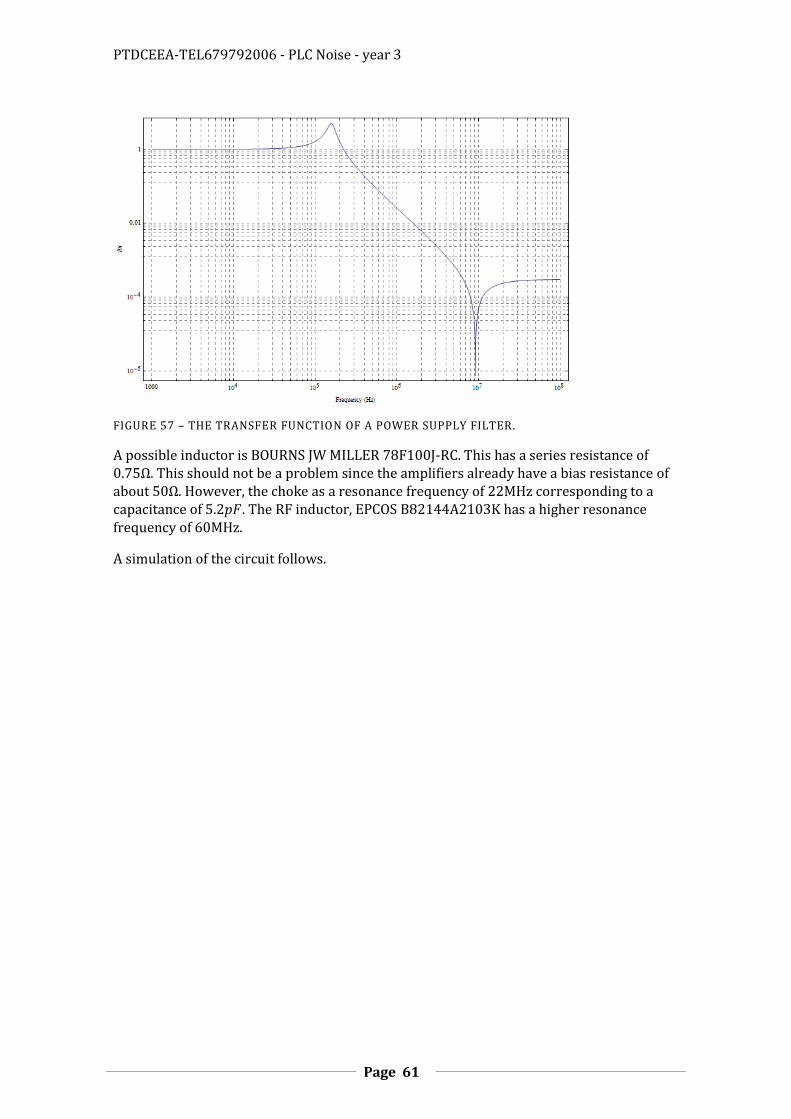
FIGURE 57 – THE TRANSFER FUNCTION OF A POWER SUPPLY FILTER.
A possible inductor is BOURNS JW MILLER 78F100J-RC. This has a series resistance of . This should not be a problem since the amplifiers already have a bias resistance of about . However, the choke as a resonance frequency of corresponding to a capacitance of . The RF inductor, EPCOS B82144A2103K has a higher resonance frequency of .
A simulation of the circuit follows.

PTDCEEA-TEL679792006 - PLC Noise - year 3
Page 62
FIGURE 58 – EQUIVALENT CIRCUIT OF A POWER SUPPLY FILTER.
This filter has the following frequency response.
FIGURE 59 – FREQUENCY RESPONSE OF THE POWER SUPPLY FILTER.
The attenuation of the filter starts decreasing at a frequency of about , since the both the L1 inductor starts to behave like its parasitic capacitance C1, and capacitor C2 and the capacitor starts behaving like its parasitic inductance L2.
Components used:
Power Supply RS: GS18A15-P1J: price, 17,08 € + 15 €
EPCOS B82144A2103K : INDUTOR, AXIAL, 10UH: preço 10 x 0.49 euros + …
UNITED CHEMI-CON KCD101E105M55A0B00: preço 10 x 1.32 euros
These are a ceramic multilayer capacitor for low series resistance. Other capacitors like Vishay BCcomponents 128 SAL-RPM is aluminum has a series resistance of for and a tantalum capacitor like AVX TACR105M025XTA has a series resistance of .
Since the ceramic capacitors are difficult to find, the circuit was changed to,
L110µH
C15.2pF
R10.75Ω
C21µF
L25nH
R250Ω
3
V1
1 Vpk
1kHz
0°
1
C3
0.6pF
5
R350Ω
6
PTDCEEA-TEL679792006 - PLC Noise - year 3
Page 63
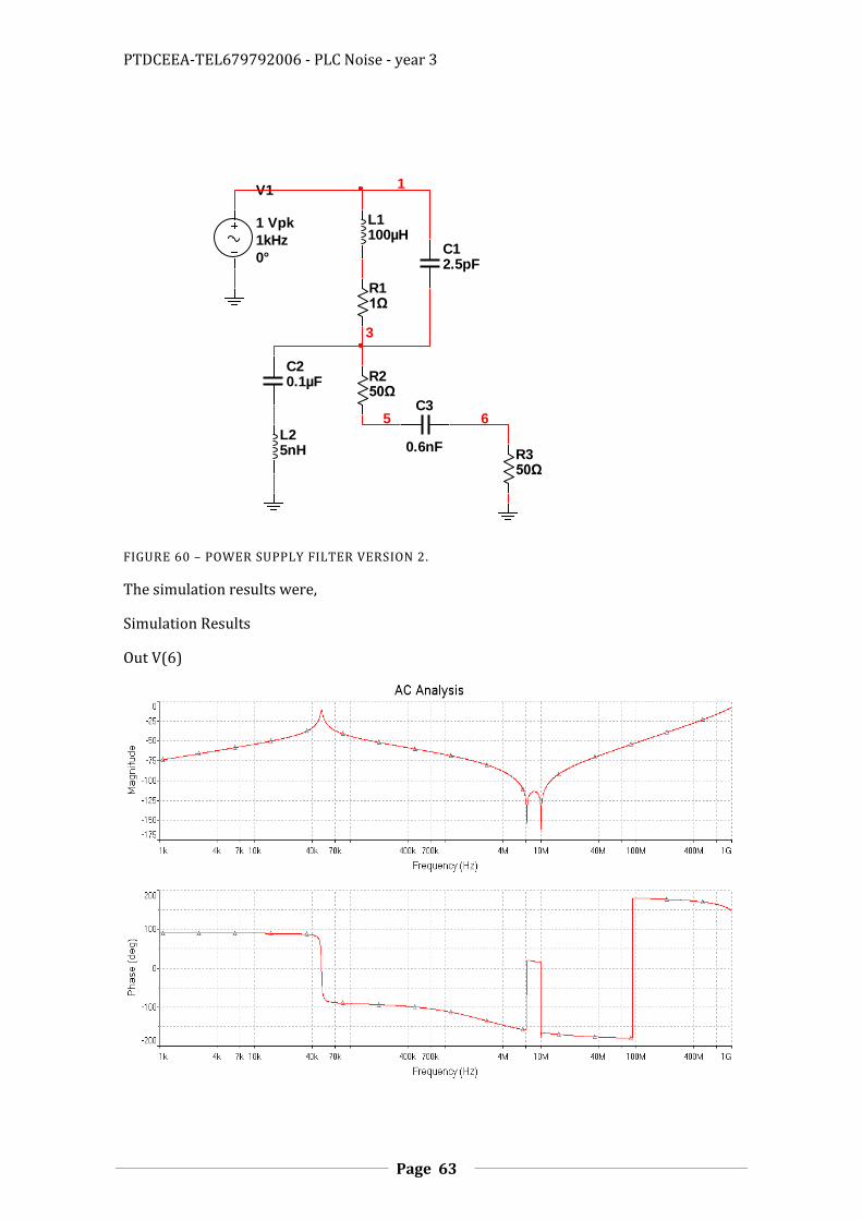
FIGURE 60 – POWER SUPPLY FILTER VERSION 2.
The simulation results were,
Simulation Results
Out V(6)
L1100µH
C12.5pF
R11Ω
C20.1µF
L25nH
R250Ω
V1
1 Vpk
1kHz
0°
1
C3
0.6nF
5
R350Ω
6
3

PTDCEEA-TEL679792006 - PLC Noise - year 3
Page 64
100MHz ->-52.2456dB
49.9015kHz-> -11.0410dB
Out V(5)
100MHz -> -52.2334dB
49.9kHz -> 29.4911dB
PICKUP CIRCUIT
In order to measure the power line noise, we developed the pickup circuit presented below:
2.2nF
2.2nF
CA
Coilcraft
Wideband Transformer SMA
Connector
220V
FIGURE 61 - PICKUP CIRCUIT USED TO MEASURE THE NOISE IN POWER LINES UP TO 500MHZ.

PTDCEEA-TEL679792006 - PLC Noise - year 3
Page 65
The 27µH inductance of the transformer and the two 2.2nF capacitors comprised a high-pass filter with cut off frequency at approximately 0.9MHz. The Frequency Response of this circuit is presented below.
FIGURE 62 - PICKUP CIRCUIT FREQUENCY RESPONSE.
ANTI-ALIASING LC FILTER
In order to cut off frequencies greater than 100MHz we used an LC filter from Coilcraft with a cut off frequency approximately 150MHZ. The frequency response of this filter is presented below. The filter is the P3LP-157L with 3 poles.
?
FIGURE 63 – MEASURED COILCRAFT LC FILTER FREQUENCY RESPONSE (WITH AN ERROR).
103
104
105
106
107
108
109
-120
-100
-80
-60
-40
-20
0
20
X: 9.441e+006
Y: 6.892
Frequency (Hz)
Magnitude (
dB
)
Pickup Circuit Frequency Response up to 500MHz
106
107
108
109
-30
-20
-10
0
10
20
30
Frequency (Hz)
Magnitude (
dB
)
Coilcraft Filter Frequency Response
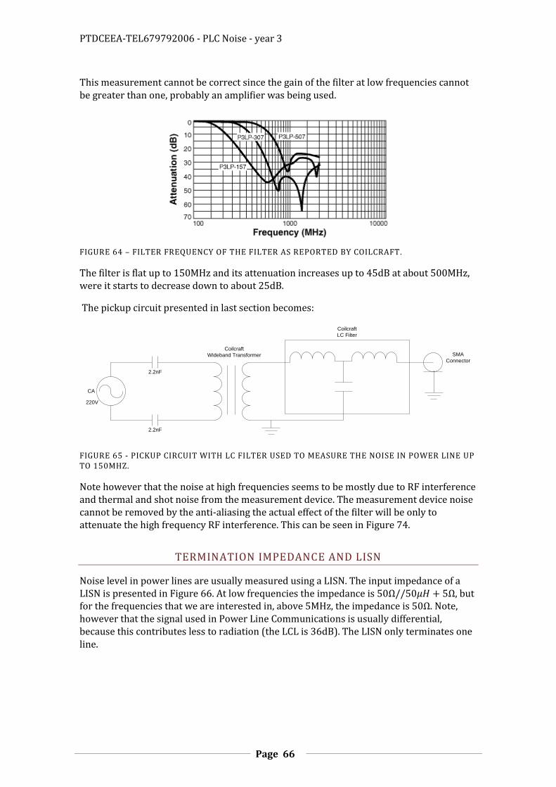
PTDCEEA-TEL679792006 - PLC Noise - year 3
Page 66
This measurement cannot be correct since the gain of the filter at low frequencies cannot be greater than one, probably an amplifier was being used.
FIGURE 64 – FILTER FREQUENCY OF THE FILTER AS REPORTED BY COILCRAFT.
The filter is flat up to 150MHz and its attenuation increases up to 45dB at about 500MHz, were it starts to decrease down to about 25dB.
The pickup circuit presented in last section becomes:
2.2nF
2.2nF
CA
Coilcraft
Wideband Transformer SMA
Connector
220V
Coilcraft
LC Filter
FIGURE 65 - PICKUP CIRCUIT WITH LC FILTER USED TO MEASURE THE NOISE IN POWER LINE UP TO 150MHZ.
Note however that the noise at high frequencies seems to be mostly due to RF interference and thermal and shot noise from the measurement device. The measurement device noise cannot be removed by the anti-aliasing the actual effect of the filter will be only to attenuate the high frequency RF interference. This can be seen in Figure 74.
TERMINATION IMPEDANCE AND LISN
Noise level in power lines are usually measured using a LISN. The input impedance of a LISN is presented in Figure 66. At low frequencies the impedance is , but for the frequencies that we are interested in, above , the impedance is . Note, however that the signal used in Power Line Communications is usually differential, because this contributes less to radiation (the LCL is 36dB). The LISN only terminates one line.

PTDCEEA-TEL679792006 - PLC Noise - year 3
Page 67
FIGURE 66 – INPUT IMPEDANCE OF A LISN.
FIGURE 67 – A CIRCUIT IMPLEMENTATION OF A LISN.
DEALING WITH THE DIFFERENT NOISE LEVELS
According to 1 the noise levels can vary from 0.03mV to 10mV in the 100MHz range. If one uses the Analog Modules 333 low noise voltage amplifier, a typical measuring setup will be,

PTDCEEA-TEL679792006 - PLC Noise - year 3
Page 68
20nF
VAC 4031X008
220 V
50 HzAM3221pF
1 2 E
PicoScope 3206
Osciloscope kit
50Ω
(46+20)pF
Lp=Ls=4uH
Lm=40uH
20nF
X1 probeM->
F—F->
M
FBNC ->
MBNC
FIGURE 68 – NOISE MEASUREMENT CIRCUIT 6TH VERSION.
The connections from amplifier to the rest of the circuit may present some problems, namely due to the parasitic inductances and capacitances. This will be analyzed later.
The Analog Modules 333 amplifier has an output voltage swing of and a gain of 100 (40dB). The signal at the output of the amplifier will vary from 3mV to 1V. The dynamic range of the noise is 1V/3mV = 300, while the allowed dynamic range at the output of the amplifier is about 5V/10mV=500.
RELATION OF THE EXPECTED NOISE LEVELS TO EMC LIMITS
In the worst case the noise will be close to the EMC limits, which also limit the MODEM signal, so the signal to noise ratio would be close to one. However, we expect that the devices noise levels be close to the EMC limit only at some specific problematic frequencies, and that the total noise level be much lower than the EMC limit.
FIGURE 69 – A MEASUREMENT A DEVICE NOISE USING AN HM6052-2 LISN.
MEASUREMENTS WITH MODULE AMPLIFIERS

PTDCEEA-TEL679792006 - PLC Noise - year 3
Page 69
20nF
WB1-1SL
220 V
50 Hz2 ZFL-5001pF
1 2 E
PicoScope 3206
Osciloscope kit
50Ω
(46+20)pF
20nF
SMA F –>
BNC M
SMA M ->
SMA F
FIGURE 70 – NOISE MEASUREMENT CIRCUIT 5TH VERSION.
The circuit above was simulated, modeling the connectors as small transmission lines.
They ideally should have and impedance of and phase velocity of √ , corresponding to the dielectric constant of common plastic Polyethylene. Since
√
And
√
These results in and .
But the lines are ideal and to simulate this we used lines with an impedance of . This results in and . We used lines to model the connectors.
To model the transform the value of the coupling factor was calculated. Since the transformer is terminated by a and the bandwidth is , and this is given by , from this results that the leakage inductance should be , the primary and secondary inductance are and since the total
inductance is , the coupling factor should be . This doesn’t takes in to account the resistive losses. The parasitic capacitances have impedances much greater than the (like ) so they this should not be relevant.
The amplifier was modeled as an ideal amplifier but with perfect output impedance and input impedance of .
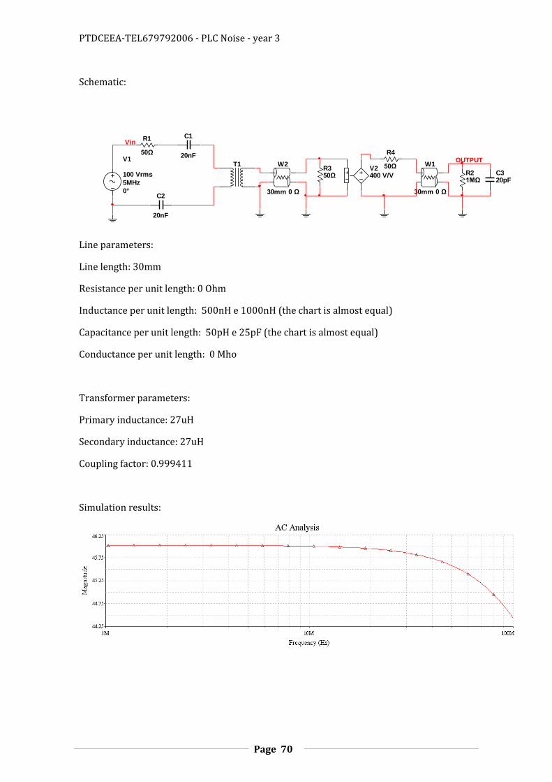
PTDCEEA-TEL679792006 - PLC Noise - year 3
Page 70
Schematic:
Line parameters:
Line length: 30mm
Resistance per unit length: 0 Ohm
Inductance per unit length: 500nH e 1000nH (the chart is almost equal)
Capacitance per unit length: 50pH e 25pF (the chart is almost equal)
Conductance per unit length: 0 Mho
Transformer parameters:
Primary inductance: 27uH
Secondary inductance: 27uH
Coupling factor: 0.999411
Simulation results:
V1
100 Vrms
5MHz
0°
R1
50Ω
C1
20nF
C2
20nF
T1 W2
30mm 0 Ω
W1
30mm 0 Ω
R21MΩ
C320pF
Vin
OUTPUT
R350Ω
V2400 V/V
R4
50Ω

PTDCEEA-TEL679792006 - PLC Noise - year 3
Page 71
FINAL MEASUREMENT SETUP
2.2nF
220 V
50 Hz ZFL500+
1 2 E
PicoScope 3206
Osciloscope kit
50Ω
Coilcraft
Wideband
Transformer
2.2nF
SMA SMA-BNC
FIGURE 71 – NOISE MEASUREMENT SETUP
The figure below shows second and final system used to measure the noise presented in Power-Lines. The Mini-circuits ZFL-500+ amplifier used previously was replaced by the Mini-Circuits ZFL-500LN+ low noise amplifiers and a 47Ω resistance was connected between the amplifiers output and the oscilloscope input, in order to prevent that the amplifier output becomes in open circuit and damaged this.
2.2nF
2.2nF
CA
Coilcraft
Wideband Transformer
SMA
Connectors
220V
Coilcraft
LC Filter
Mini-Circuits
ZFL-500LN+
SMA
Connectors
GNDVCC
15V
100μH100nF
Out
47Ω
FIGURE 72 – FINAL SYSTEM USED IN PLC NOISE MEASURE.
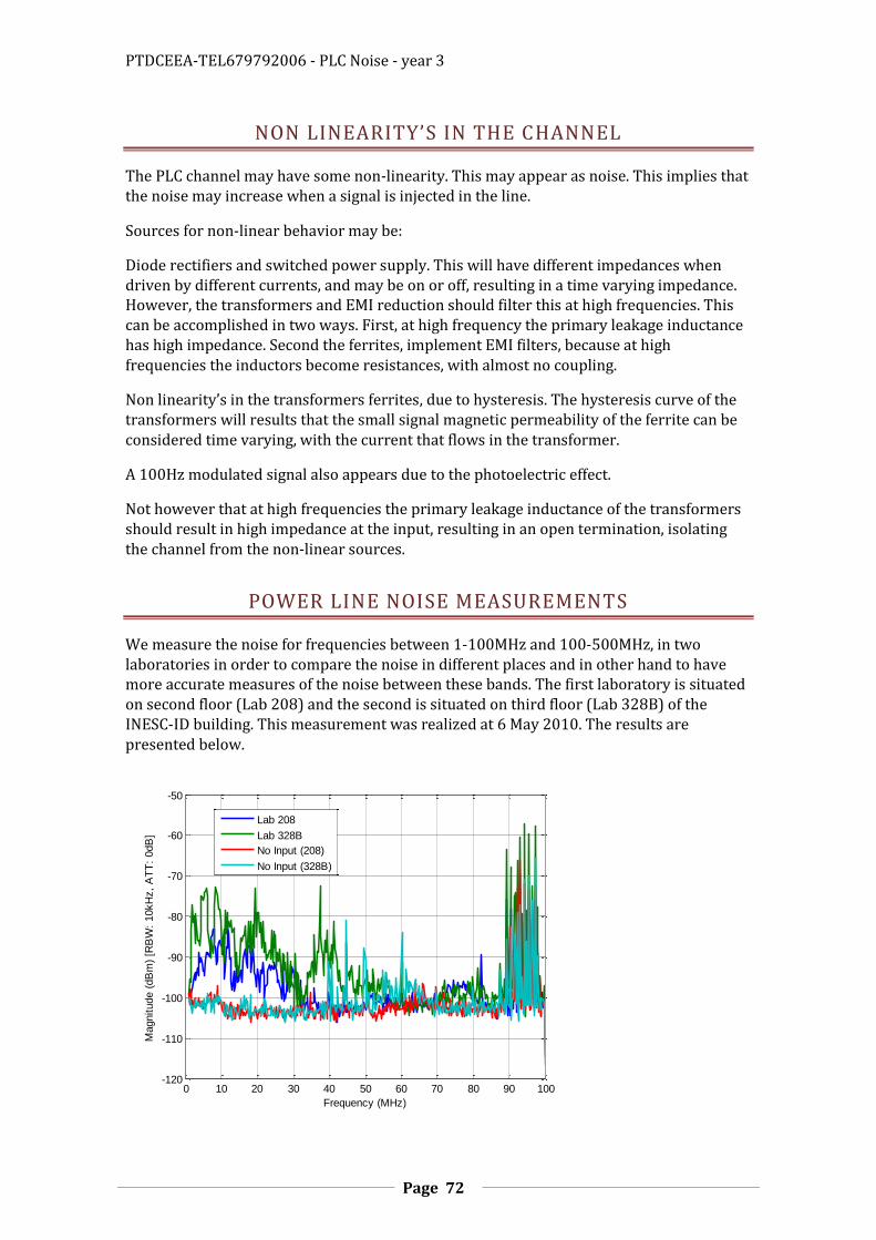
PTDCEEA-TEL679792006 - PLC Noise - year 3
Page 72
NON LINEARITY’S IN THE CHANNEL
The PLC channel may have some non-linearity. This may appear as noise. This implies that the noise may increase when a signal is injected in the line.
Sources for non-linear behavior may be:
Diode rectifiers and switched power supply. This will have different impedances when driven by different currents, and may be on or off, resulting in a time varying impedance. However, the transformers and EMI reduction should filter this at high frequencies. This can be accomplished in two ways. First, at high frequency the primary leakage inductance has high impedance. Second the ferrites, implement EMI filters, because at high frequencies the inductors become resistances, with almost no coupling.
Non linearity’s in the transformers ferrites, due to hysteresis. The hysteresis curve of the transformers will results that the small signal magnetic permeability of the ferrite can be considered time varying, with the current that flows in the transformer.
A 100Hz modulated signal also appears due to the photoelectric effect.
Not however that at high frequencies the primary leakage inductance of the transformers should result in high impedance at the input, resulting in an open termination, isolating the channel from the non-linear sources.
POWER LINE NOISE MEASUREMENTS
We measure the noise for frequencies between 1-100MHz and 100-500MHz, in two laboratories in order to compare the noise in different places and in other hand to have more accurate measures of the noise between these bands. The first laboratory is situated on second floor (Lab 208) and the second is situated on third floor (Lab 328B) of the INESC-ID building. This measurement was realized at 6 May 2010. The results are presented below.
0 10 20 30 40 50 60 70 80 90 100-120
-110
-100
-90
-80
-70
-60
-50
Frequency (MHz)
Magnitude (
dB
m)
[RB
W:
10kH
z,
AT
T:
0dB
]
Noise Spectrum up to 100MHz
Lab 208
Lab 328B
No Input (208)
No Input (328B)
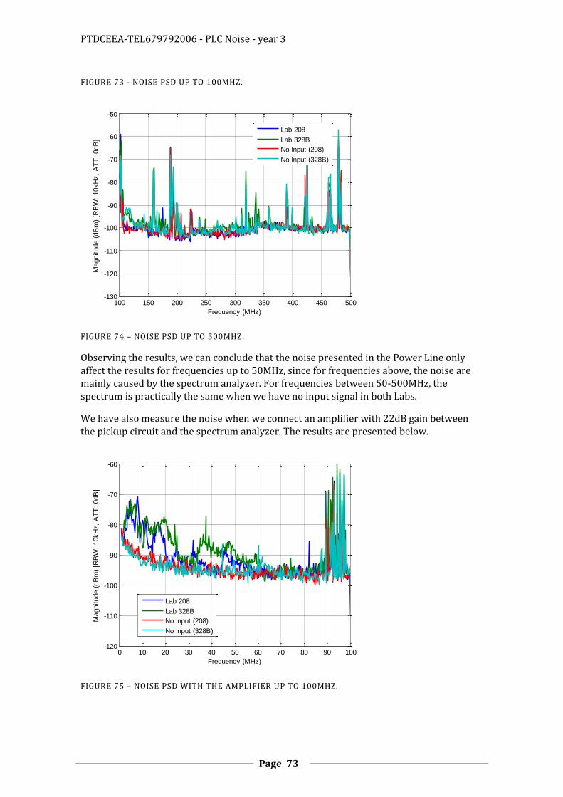
PTDCEEA-TEL679792006 - PLC Noise - year 3
Page 73
FIGURE 73 - NOISE PSD UP TO 100MHZ.
FIGURE 74 – NOISE PSD UP TO 500MHZ.
Observing the results, we can conclude that the noise presented in the Power Line only affect the results for frequencies up to 50MHz, since for frequencies above, the noise are mainly caused by the spectrum analyzer. For frequencies between 50-500MHz, the spectrum is practically the same when we have no input signal in both Labs.
We have also measure the noise when we connect an amplifier with 22dB gain between the pickup circuit and the spectrum analyzer. The results are presented below.
FIGURE 75 – NOISE PSD WITH THE AMPLIFIER UP TO 100MHZ.
100 150 200 250 300 350 400 450 500-130
-120
-110
-100
-90
-80
-70
-60
-50
Frequency (MHz)
Magnitude (
dB
m)
[RB
W:
10kH
z,
AT
T:
0dB
]
Noise Spectrum up to 500MHz
Lab 208
Lab 328B
No Input (208)
No Input (328B)
0 10 20 30 40 50 60 70 80 90 100-120
-110
-100
-90
-80
-70
-60
Frequency (MHz)
Magnitude (
dB
m)
[RB
W:
10kH
z,
AT
T:
0dB
]
Noise Spectrum with Amplifier up to 100MHz
Lab 208
Lab 328B
No Input (208)
No Input (328B)
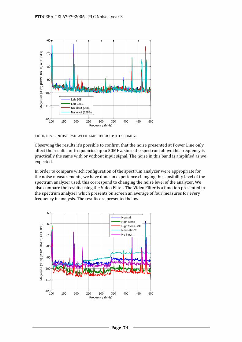
PTDCEEA-TEL679792006 - PLC Noise - year 3
Page 74
FIGURE 76 – NOISE PSD WITH AMPLIFIER UP TO 500MHZ.
Observing the results it’s possible to confirm that the noise presented at Power Line only affect the results for frequencies up to 50MHz, since the spectrum above this frequency is practically the same with or without input signal. The noise in this band is amplified as we expected.
In order to compare witch configuration of the spectrum analyzer were appropriate for the noise measurements, we have done an experience changing the sensibility level of the spectrum analyzer used, this correspond to changing the noise level of the analyzer. We also compare the results using the Video Filter. The Video Filter is a function presented in the spectrum analyzer which presents on screen an average of four measures for every frequency in analysis. The results are presented below.
100 150 200 250 300 350 400 450 500-120
-110
-100
-90
-80
-70
-60
Frequency (MHz)
Magnitude (
dB
m)
[RB
W:
10kH
z,
AT
T:
0dB
]
Noise Spectrum with Amplifier up to 500MHz
Lab 208
Lab 328B
No Input (208)
No Input (328B)
100 150 200 250 300 350 400 450 500-120
-110
-100
-90
-80
-70
-60
-50
Frequency (MHz)
Magnitude (
dB
m)
[RB
W:
10kH
z,
AT
T:
0dB
]
Noise Spectrum up to 500MHz (Lab 208)
Normal
High Sens
High Sens+VF
Normal+VF
No Input

PTDCEEA-TEL679792006 - PLC Noise - year 3
Page 75
FIGURE 77 – MEASUREMENTS WITH DIFFERENT CONFIGURATIONS OF THE SPECTRUM ANALYZER.
The results above were taken without the amplifier connected between the pickup circuit and the spectrum analyzer.
FIGURE 78 – MEASUREMENTS WITH DIFFERENT CONFIGURATIONS OF THE SPECTRUM ANALYZER.
This measure was done with one amplifier connected between the pickup circuit and the Spectrum analyzer.
Observing the results, we chose the High Sensibility mode to execute our measures. This results in lower internal noise of the spectrum analyzer.
Using the LC anti-aliasing filter presented previously, we had measure the noise spectrum from 1-500MHz with and without connecting the pickup circuit to AC mains. These measures were taken on 7 May 2010.
100 150 200 250 300 350 400 450 500-130
-120
-110
-100
-90
-80
-70
-60
-50
Frequency (MHz)
Magnitude (
dB
m)
[RB
W:
10kH
z,
AT
T:
0dB
]
Noise Spectrum with Amplifier up to 500MHz (Lab 208)
Normal
High Sens
High Sens+VF
Normal+VF
No Input

PTDCEEA-TEL679792006 - PLC Noise - year 3
Page 76
FIGURE 79 - NOISE PSD WITH LC FILTER.
These results were taken without the amplifier connected between the pickup circuit and the spectrum analyzer.
After analysis in frequency with the spectrum analyzer, we have measure the noise with a digital storage oscilloscope (DSO). The DSO used was the PicoScope 3206 witch can digitized to 8bits and is capable of recording 1 million samples with rate of 200Msamples/sec. The result is presented below:
FIGURE 80 - NOISE MEASUREMENT IN TIME.
The figure above present only 0.05ms of 5ms measured, with the DSO referred, at 200Msamples/s. This measure was taken with two amplifiers in cascade between the pickup circuit and the DSO.
0 50 100 150 200 250 300 350 400 450 500-120
-110
-100
-90
-80
-70
-60
Frequency (MHz)
Magnitude (
dB
) [R
BW
: 10kH
z,
AT
T:
0dB
]
Noise Spectrum with Filter
With Input Signal
Without Input Signal
0 0.005 0.01 0.015 0.02 0.025 0.03 0.035 0.04 0.045 0.05-0.5
-0.4
-0.3
-0.2
-0.1
0
0.1
0.2
0.3
0.4
Time (ms)
Am
plit
ude (
V)
[200M
sam
ple
s/s
ec,
1M
sam
ple
, 5m
s]
Noise Measure (with two amplifiers)
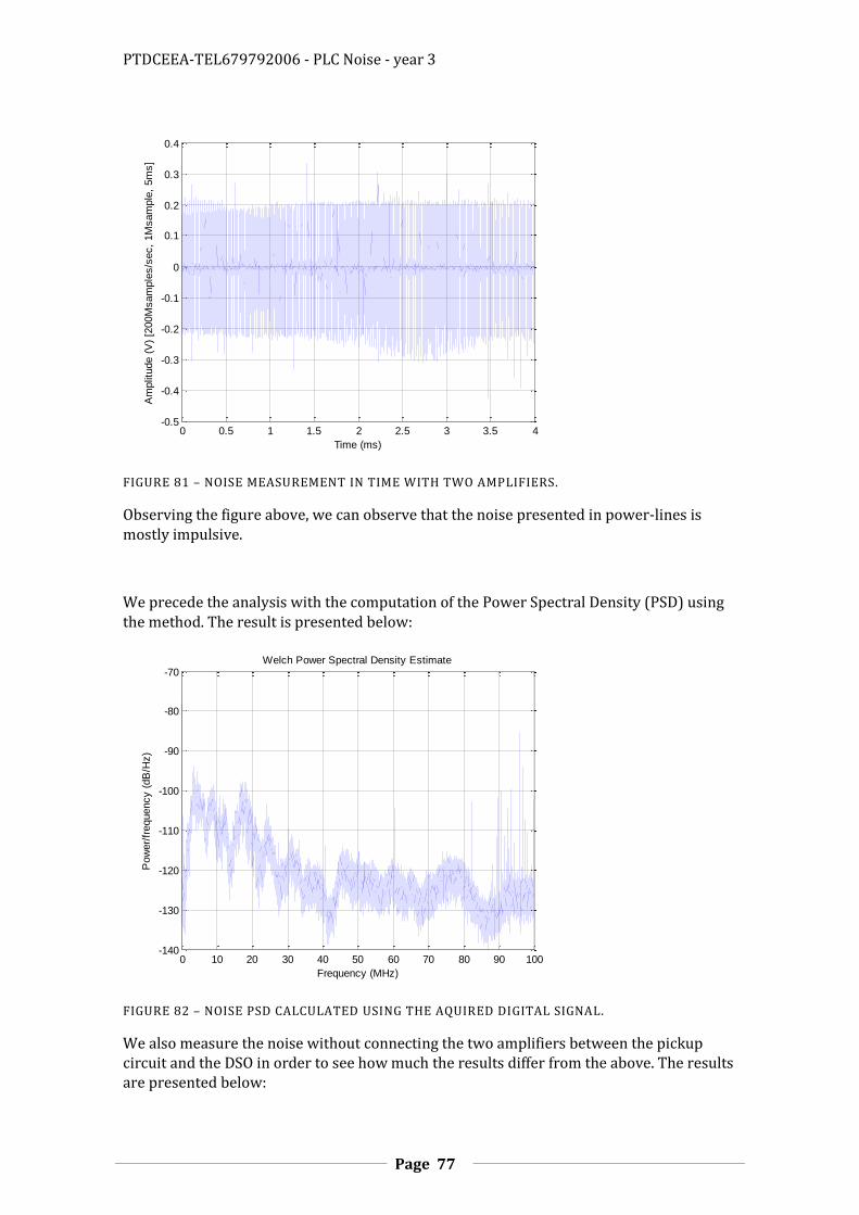
PTDCEEA-TEL679792006 - PLC Noise - year 3
Page 77
FIGURE 81 – NOISE MEASUREMENT IN TIME WITH TWO AMPLIFIERS.
Observing the figure above, we can observe that the noise presented in power-lines is mostly impulsive.
We precede the analysis with the computation of the Power Spectral Density (PSD) using the method. The result is presented below:
FIGURE 82 – NOISE PSD CALCULATED USING THE AQUIRED DIGITAL SIGNAL.
We also measure the noise without connecting the two amplifiers between the pickup circuit and the DSO in order to see how much the results differ from the above. The results are presented below:
0 0.5 1 1.5 2 2.5 3 3.5 4-0.5
-0.4
-0.3
-0.2
-0.1
0
0.1
0.2
0.3
0.4
Time (ms)
Am
plit
ude (
V)
[200M
sam
ple
s/s
ec,
1M
sam
ple
, 5m
s]
Noise Measure (with two amplifiers)
0 10 20 30 40 50 60 70 80 90 100-140
-130
-120
-110
-100
-90
-80
-70
Frequency (MHz)
Pow
er/
frequency (
dB
/Hz)
Welch Power Spectral Density Estimate

PTDCEEA-TEL679792006 - PLC Noise - year 3
Page 78
FIGURE 83 - NOISE MEASURE WITHOUT AMPLIFIERS.
And the PSD becomes,
FIGURE 84 - POWER SPECTRAL DENSITY WITHOUT AMPLIFIER.
To confirm the results above we have done two measurements with only one of two amplifiers connected between the pickup circuit and the DSO. These results are presented below.
0 0.05 0.1 0.15 0.2 0.25 0.3 0.35 0.4 0.45 0.5-30
-25
-20
-15
-10
-5
0
5
10
15
20
Time (ms)
Am
plit
ude (
mV
) [2
00M
sam
ple
s/s
ec,
1M
sam
ple
, 5m
s]
Noise Measure Without Amplifier
0 10 20 30 40 50 60 70 80 90 100-150
-140
-130
-120
-110
-100
-90
-80
Frequency (MHz)
Pow
er/
frequency (
dB
/Hz)
Welch Power Spectral Density Estimate

PTDCEEA-TEL679792006 - PLC Noise - year 3
Page 79
FIGURE 85 - NOISE MEASUREMENT WITH ONLY AMPLIFIER 1.
FIGURE 86 - NOISE MEASUREMENT WITH ONLY AMPLIFIER 2.
To compare the noise presented in a home environment relatively to those presented in a Laboratory, we have done a measurement in a house a compare this results with those obtains in the laboratory. These measurements were taken on 24/05/2010 at home and also at the lab.
0 0.05 0.1 0.15 0.2 0.25 0.3 0.35 0.4 0.45 0.5-40
-30
-20
-10
0
10
20
30
Time (ms)
Am
plit
ude (
mV
) [2
00M
sam
ple
s/s
ec,
1M
sam
ple
, 5m
s]
Noise Measure (One Amplifier1)
0 0.05 0.1 0.15 0.2 0.25 0.3 0.35 0.4 0.45 0.5-30
-25
-20
-15
-10
-5
0
5
10
15
20
Time (ms)
Am
plit
ude (
mV
) [2
00M
sam
ple
s/s
ec,
1M
sam
ple
, 5m
s]
Noise Measure (One Amplifier2)

PTDCEEA-TEL679792006 - PLC Noise - year 3
Page 80
FIGURE 87 - COMPARISON OF THE NOISE AT HOUSE WITH THE NOISE AT LABORATORY.
We also try measuring the noise with another DSO. So we choose the TEKTRONIX TDS3054B. This result is presented below:
FIGURE 88 - NOISE MEASURE WITH TEKTRONIX TDS3054B.
and the PSD becomes,
0 0.05 0.1 0.15 0.2 0.25 0.3 0.35 0.4 0.45 0.5-30
-25
-20
-15
-10
-5
0
5
10
15
20
Time (ms)
Am
plit
ude (
mV
) [2
00M
sam
ple
s/s
ec,
1M
sam
ple
, 5m
s]
Noise Measure Without Amplifier [24/05/10 (Lab and House)]
Laboratory
House
0 5 10 15 20 25 30 35 40-15
-10
-5
0
5
10
15
Time (s)
Am
plit
ude (
mV
)
Noise Measure with Tektronix TDS3054B
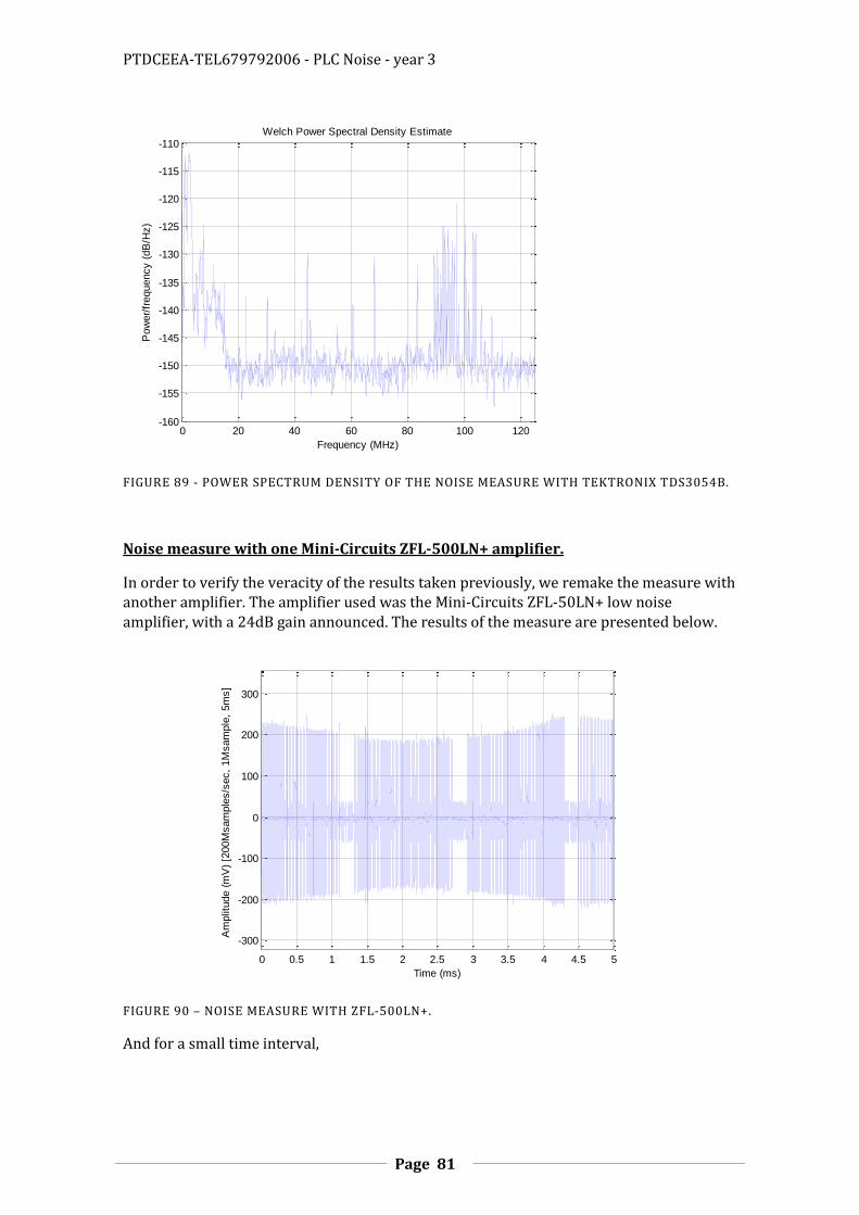
PTDCEEA-TEL679792006 - PLC Noise - year 3
Page 81
FIGURE 89 - POWER SPECTRUM DENSITY OF THE NOISE MEASURE WITH TEKTRONIX TDS3054B.
Noise measure with one Mini-Circuits ZFL-500LN+ amplifier.
In order to verify the veracity of the results taken previously, we remake the measure with another amplifier. The amplifier used was the Mini-Circuits ZFL-50LN+ low noise amplifier, with a 24dB gain announced. The results of the measure are presented below.
FIGURE 90 – NOISE MEASURE WITH ZFL-500LN+.
And for a small time interval,
0 20 40 60 80 100 120-160
-155
-150
-145
-140
-135
-130
-125
-120
-115
-110
Frequency (MHz)
Pow
er/
frequency (
dB
/Hz)
Welch Power Spectral Density Estimate
0 0.5 1 1.5 2 2.5 3 3.5 4 4.5 5
-300
-200
-100
0
100
200
300
Time (ms)
Am
plit
ude (
mV
) [2
00M
sam
ple
s/s
ec,
1M
sam
ple
, 5m
s]
Noise Measure (with one amplifier ZFL-500LN)

PTDCEEA-TEL679792006 - PLC Noise - year 3
Page 82
FIGURE 91 – NOISE MEASURE IN A SMALL TIME INTERVAL.
This measure with only one new amplifier connecting between the oscilloscope and the pick-up circuit developed previously. The oscilloscope used was also the PicoScope configured to sample at rate 200Msamples/s.
The power spectral density is presented below.
FIGURE 92 – POWER SPECTRAL DENSITY OF THE MEASURE WITH ZFL-500LN.
0 0.005 0.01 0.015 0.02 0.025 0.03 0.035 0.04 0.045 0.05-300
-200
-100
0
100
200
300
Time (ms)
Am
plit
ude (
mV
) [2
00M
sam
ple
s/s
ec,
1M
sam
ple
, 5m
s]
Noise Measure (with one amplifier ZFL-500LN)
0 10 20 30 40 50 60 70 80 90 100-200
-180
-160
-140
-120
-100
-80
-60
Frequency (MHz)
Pow
er/
frequency (
dB
/Hz)
Power Spectral Density
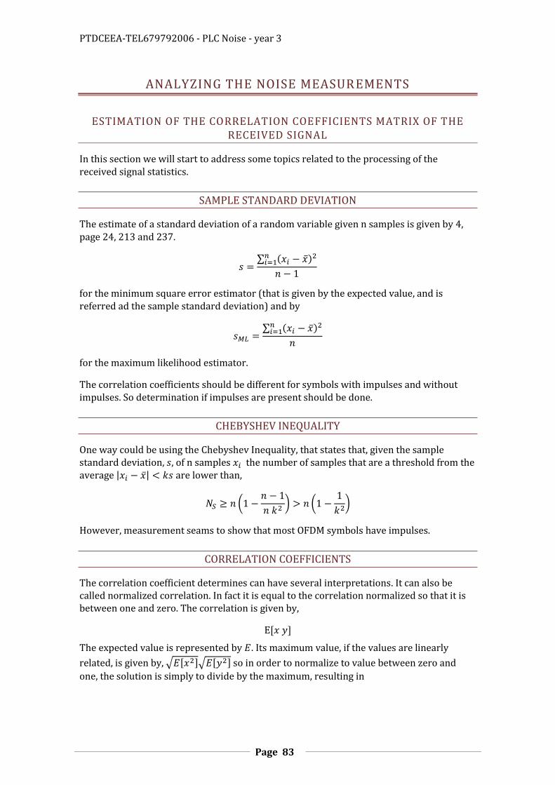
PTDCEEA-TEL679792006 - PLC Noise - year 3
Page 83
ANALYZING THE NOISE MEASUREMENTS
ESTIMATION OF THE CORRELATION COEFFICIENTS MATRIX OF THE RECEIVED SIGNAL
In this section we will start to address some topics related to the processing of the received signal statistics.
SAMPLE STANDARD DEVIATION
The estimate of a standard deviation of a random variable given n samples is given by 4, page 24, 213 and 237.
∑
for the minimum square error estimator (that is given by the expected value, and is referred ad the sample standard deviation) and by
∑
for the maximum likelihood estimator.
The correlation coefficients should be different for symbols with impulses and without impulses. So determination if impulses are present should be done.
CHEBYSHEV INEQUALITY
One way could be using the Chebyshev Inequality, that states that, given the sample standard deviation, , of n samples the number of samples that are a threshold from the average | | are lower than,
(
) (
)
However, measurement seams to show that most OFDM symbols have impulses.
CORRELATION COEFFICIENTS
The correlation coefficient determines can have several interpretations. It can also be called normalized correlation. In fact it is equal to the correlation normalized so that it is between one and zero. The correlation is given by,
The expected value is represented by . Its maximum value, if the values are linearly
related, is given by, √ √ so in order to normalize to value between zero and
one, the solution is simply to divide by the maximum, resulting in

PTDCEEA-TEL679792006 - PLC Noise - year 3
Page 84
√
That is the correlation coefficient or the normalized correlation.
If the correlation is taken as dot product in some linear space then the correlation coefficient is juts the cosine of the angle between the two signals. Note the projection of the vector A into vector B is given by with | |.
The correlation coefficients are a measure of similarity. If the signals are taken to be formed by , and , then correlation coefficient is the energy of the signal divided by the geometric average of the energy of signal and .
√
Also if you are trying to estimate linearly from using , and minimizing the mean square error, , then,
√
And the residual error will be given by
So, the correlation coefficient is related to the residual error as a fraction of the desired signal.
COMPLEX CORRELATION COEFFICIENTS
Defining the complex variables,
And minimizing,
| |
By solving the system,
and
Results in
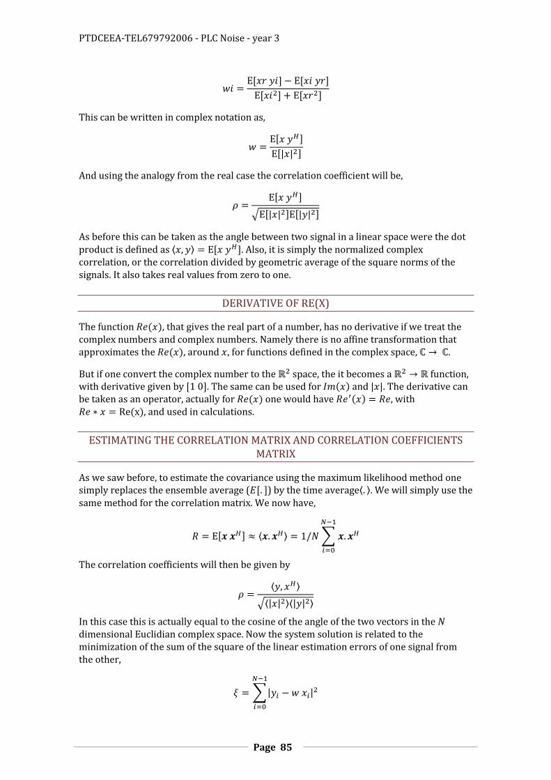
PTDCEEA-TEL679792006 - PLC Noise - year 3
Page 85
This can be written in complex notation as,
| |
And using the analogy from the real case the correlation coefficient will be,
√ | | | |
As before this can be taken as the angle between two signal in a linear space were the dot product is defined as ⟨ ⟩ . Also, it is simply the normalized complex correlation, or the correlation divided by geometric average of the square norms of the signals. It also takes real values from zero to one.
DERIVATIVE OF RE(X)
The function , that gives the real part of a number, has no derivative if we treat the complex numbers and complex numbers. Namely there is no affine transformation that approximates the , around , for functions defined in the complex space, .
But if one convert the complex number to the space, the it becomes a function, with derivative given by . The same can be used for and | |. The derivative can be taken as an operator, actually for one would have , with , and used in calculations.
ESTIMATING THE CORRELATION MATRIX AND CORRELATION COEFFICIENTS MATRIX
As we saw before, to estimate the covariance using the maximum likelihood method one simply replaces the ensemble average ( ) by the time average⟨ ⟩. We will simply use the
same method for the correlation matrix. We now have,
⟨ ⟩ ∑
The correlation coefficients will then be given by
⟨ ⟩
√⟨| | ⟩⟨| | ⟩
In this case this is actually equal to the cosine of the angle of the two vectors in the dimensional Euclidian complex space. Now the system solution is related to the minimization of the sum of the square of the linear estimation errors of one signal from the other,
∑| |

PTDCEEA-TEL679792006 - PLC Noise - year 3
Page 86
The resulting matrix of correlation coefficients will be given by,
⟨ ⟩
√⟨| | ⟩⟨| | ⟩
√
Or still, defining as the vector formed by the main diagonal of , as,
√
Were the division is element wise.
PTDCEEA-TEL679792006 - PLC Noise - year 3
Page 87
ESTIMATION OF THE CORRELATION COEFFICIENTS MATRIX OF THE COMPENSATED OFDM SIGNAL VERSION ONE
The received OFDM signal will be converted to baseband, the circular prefix will be removed and the DFT will be calculated using the FFT. We would like to determine the covariance matrix of the received vector. To simplify the calculations, however we will initially skip the demodulation and the removal of the circular prefix. We will simply obtain the FFT of each received signal and then estimate the covariance of this vector. This will result in an estimate of the actual covariance matrix.
We have a set of received signals OFDM symbols given by,
The received signal will be processed. And the received vector covariance matrix can be calculated by,
And
∑
This can be calculated in a more efficient way by formatting the received signal as a matrix and multiplying by its Hermitian transpose. The result will be more or less the same as if we calculate the covariance in time domain and then make a coordinate transform to the domain of the DFT transform, however this
The correlation coefficient matrix, , is then given by,
√
That comes from,
∑
∑ √
However, in the calculations the average was not removed. The actual signals in the frequency domain in general should have zero mean, so the difference should not be too important, however it can happen that if a constant sinusoidal signal is presented, that is synchronized with the OFDM symbol the result will also be constant, and so the signal will not have zero mean. In this case the bias in the signal should count as noise, so it should not be removed. We are in fact assuming that the signal has zero mean and we are counting the bias as variance.
Resolving the equation above in order to ,
PTDCEEA-TEL679792006 - PLC Noise - year 3
Page 88
So the left side is proportional to were is the proportionality constant. This can estimated using the sample values. The value that minimizes the square between the predicted value for the phase given and the phase,
∑ | ( )
– |
will be given by,
∑ (
) (
)
∑ (
)
(pos1)
where is the angle, in radians, of the OFDM symbols, the OFDM symbols mean
phase and the dimension of OFDM symbol. In order to estimate , one must use the unwrapped version of the angle, that is, without the module that results from estimation form the complex amplitude. In order to do this one must be sure that the angle does not change more than, from carrier to carrier . If this is accurate then one can estimate with no error, and accurately estimate the unwrapped phase. This does not happen if we use the normal version of . In order to achieve is, one should use something like and , in order to reduce the phase variation. The vector length will be equal to times the length of , and can be calculated by
* ( )
+
Were is column vector with zeros, and , is the extension of the row vector , with the row vector . A value of 2 was used for , this assures that the phase variation between carries is bellow , as show in the following section. The unwrap
function used assumes that the phase variation is between – and . Similar results should also be obtained for equal to one and using an unwrap function that assumes that the phase variation is negative, (between and 0). Note that this is the phase variation and not the phase, (see following section).
The given formula accurately estimates impulse position, . However, it uses the formula for the correlation coefficient between two variables and . in this special case we have , so it may be possible to simplify the formula. Instead of minimizing the difference between the phase (unwrapped) and the predicted value for the phase, one could minimize the difference between the phase variation and the predicted phase variation.
∑ |
|
This is a different optimization problem.
It will result that the impulse position will be related to the average phase variation,
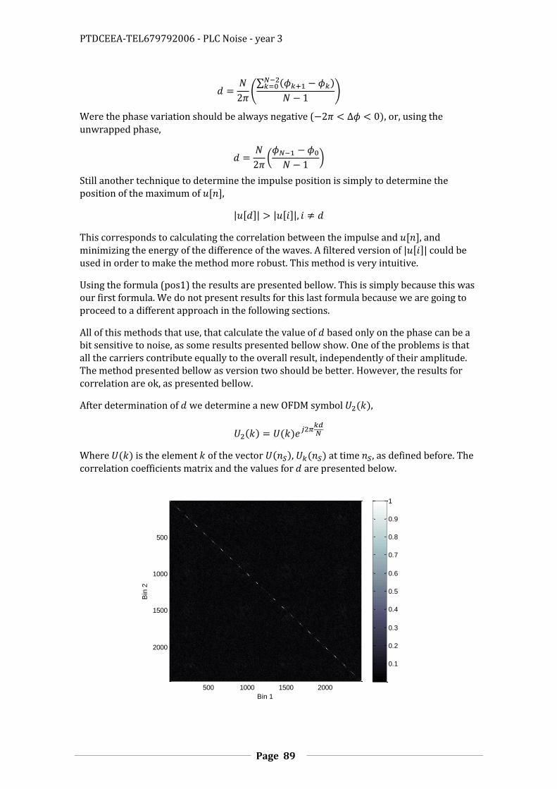
PTDCEEA-TEL679792006 - PLC Noise - year 3
Page 89
(∑
)
Were the phase variation should be always negative ( , or, using the
unwrapped phase,
(
)
Still another technique to determine the impulse position is simply to determine the position of the maximum of ,
| | | |
This corresponds to calculating the correlation between the impulse and , and minimizing the energy of the difference of the waves. A filtered version of | | could be used in order to make the method more robust. This method is very intuitive.
Using the formula (pos1) the results are presented bellow. This is simply because this was our first formula. We do not present results for this last formula because we are going to proceed to a different approach in the following sections.
All of this methods that use, that calculate the value of based only on the phase can be a bit sensitive to noise, as some results presented bellow show. One of the problems is that all the carriers contribute equally to the overall result, independently of their amplitude. The method presented bellow as version two should be better. However, the results for correlation are ok, as presented bellow.
After determination of we determine a new OFDM symbol ,
Where is the element of the vector , at time , as defined before. The
correlation coefficients matrix and the values for are presented below.
Bin 1
Bin
2
Correlation Coefficients Matrix with 1 Noise Measured Waveform
500 1000 1500 2000
500
1000
1500
2000
0.1
0.2
0.3
0.4
0.5
0.6
0.7
0.8
0.9
1
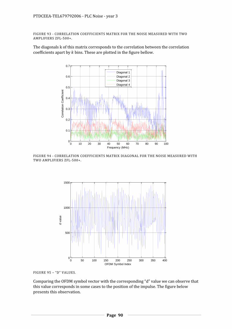
PTDCEEA-TEL679792006 - PLC Noise - year 3
Page 90
FIGURE 93 - CORRELATION COEFFICIENTS MATRIX FOR THE NOISE MEASURED WITH TWO AMPLIFIERS ZFL-500+.
The diagonals k of this matrix corresponds to the correlation between the correlation coefficients apart by bins. These are plotted in the figure bellow.
FIGURE 94 - CORRELATION COEFFICIENTS MATRIX DIAGONAL FOR THE NOISE MEASURED WITH TWO AMPLIFIERS ZFL-500+.
FIGURE 95 – “D” VALUES.
Comparing the OFDM symbol vector with the corresponding “d” value we can observe that this value corresponds in some cases to the position of the impulse. The figure below presents this observation.
0 10 20 30 40 50 60 70 80 90 1000
0.1
0.2
0.3
0.4
0.5
0.6
0.7
Frequency (MHz)
Corr
ela
tion C
oeff
icie
nt
Correlation Coefficients Matrix Diagonal with 1 Noise Measured Waveform
Diagonal 1
Diagonal 2
Diagonal 3
Diagonal 4
0 50 100 150 200 250 300 350 4000
500
1000
1500
OFDM Symbol Index
d v
alu
e
d values

PTDCEEA-TEL679792006 - PLC Noise - year 3
Page 91
FIGURE 96 – COMPARISON OF THE OFDM SYMBOL VECTOR AND THE CORRESPONDING “D” VALUE.
Next we represent figure above separately.
1st Impulse with corresponding “d” value:
FIGURE 97 – IMPULSE 1 WITH CORRESPONDING “D” VALUE.
0 500 1000 1500 2000 2500
-0.2
0
0.2
OFDM Symbol Index
Am
plit
ude (
V)
Impulse 1
0 500 1000 1500 2000 2500
-0.2
0
0.2
OFDM Symbol Index
Am
plit
ude (
V)
Impulse 4
0 500 1000 1500 2000 2500
-0.2
0
0.2
OFDM Symbol Index
Am
plit
ude (
V)
Impulse 120
Impulse
"d" Value"
Impulse
"d" Value"
Impulse
"d" Value"
0 500 1000 1500 2000 2500
-0.25
-0.2
-0.15
-0.1
-0.05
0
0.05
0.1
0.15
0.2
0.25
OFDM Symbol Index
Am
plit
ude (
V)
Impulse 1
Impulse
"d" Value"

PTDCEEA-TEL679792006 - PLC Noise - year 3
Page 92
4th Impulse with corresponding “d” value:
FIGURE 98 – IMPULSE 4WITH CORRESPONDING “D” VALUE.
120th Impulse with corresponding “d” value:
FIGURE 99 – IMPULSE 120 WITH CORRESPONDING “D” VALUE .
The Figures above represents cases were the value of “d” corresponds exactly with the position of the impulse. This isn’t true for every “d” value as we can see in Figures below.
0 500 1000 1500 2000 2500
-0.25
-0.2
-0.15
-0.1
-0.05
0
0.05
0.1
0.15
0.2
0.25
OFDM Symbol Index
Am
plit
ude (
V)
Impulse 4
Impulse
"d" Value"
0 500 1000 1500 2000 2500
-0.25
-0.2
-0.15
-0.1
-0.05
0
0.05
0.1
0.15
0.2
0.25
OFDM Symbol Index
Am
plit
ude (
V)
Impulse 120
Impulse
"d" Value"

PTDCEEA-TEL679792006 - PLC Noise - year 3
Page 93
FIGURE 100 - COMPARISION OF THE OFDM SYMBOL VECTOR AND THE CORRESPONDING “D” VALUE FOR CASES WERE “D” DOESN’T MATCHS THE IMPULSE POSITIONS.
Next we present the same Figure above separately as done before.
2nd Impulse with corresponding “d” value:
FIGURE 101 - IMPULSE 2 WITH CORRESPONDING “D” VALUE.
141th Impulse with corresponding “d” value:
0 500 1000 1500 2000 2500
-0.20
0.2
OFDM Symbol Index
Am
plit
ude (
V) Impulse 2
Impulse
"d" Value
0 500 1000 1500 2000 2500
-0.20
0.2
OFDM Symbol Index
Am
plit
ude (
V) Impulse 141
Impulse
"d" Value
0 500 1000 1500 2000 2500
-0.20
0.2
OFDM Symbol Index
Am
plit
ude (
V) Impulse 179
Impulse
"d" Value
0 500 1000 1500 2000 2500
-0.25
-0.2
-0.15
-0.1
-0.05
0
0.05
0.1
0.15
0.2
0.25
OFDM Symbol Index
Am
plit
ude (
V)
Impulse 2
Impulse
"d" Value

PTDCEEA-TEL679792006 - PLC Noise - year 3
Page 94
FIGURE 102 - IMPULSE 141 WITH CORRESPONDING “D” VALUE .
179th Impulse with corresponding “d” value:
FIGURE 103 - IMPULSE 179 WITH CORRESPONDING “D” VALUE .
PHASE VARIATION WITH K
The phase variation the transform domain signal, ,
with, , given by,
0 500 1000 1500 2000 2500
-0.25
-0.2
-0.15
-0.1
-0.05
0
0.05
0.1
0.15
0.2
0.25
OFDM Symbol Index
Am
plit
ude (
V)
Impulse 141
Impulse
"d" Value
0 500 1000 1500 2000 2500
-0.25
-0.2
-0.15
-0.1
-0.05
0
0.05
0.1
0.15
0.2
0.25
OFDM Symbol Index
Am
plit
ude (
V)
Impulse 179
Impulse
"d" Value
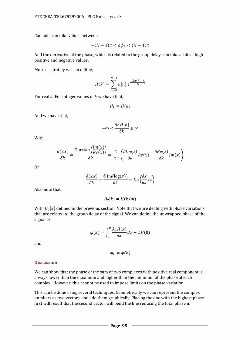
PTDCEEA-TEL679792006 - PLC Noise - year 3
Page 95
Can take can take values between
And the derivative of the phase, which is related to the group delay, can take arbitral high positive and negative values.
More accurately we can define,
∑
For real . For integer values of we have that,
And we have that,
With
(
)
| | (
)
Or
Im
(
)
Also note that,
With defined in the previous section. Note that we are dealing with phase variations that are related to the group delay of the signal. We can define the unwrapped phase of the signal as,
∫
and
Discussion
We can show that the phase of the sum of two complexes with positive real component is always lower than the maximum and higher than the minimum of the phase of each complex. However, this cannot be used to impose limits on the phase variation.
This can be done using several techniques. Geometrically we can represent the complex numbers as two vectors, and add them graphically. Placing the one with the highest phase first will result that the second vector will bend the line reducing the total phase in
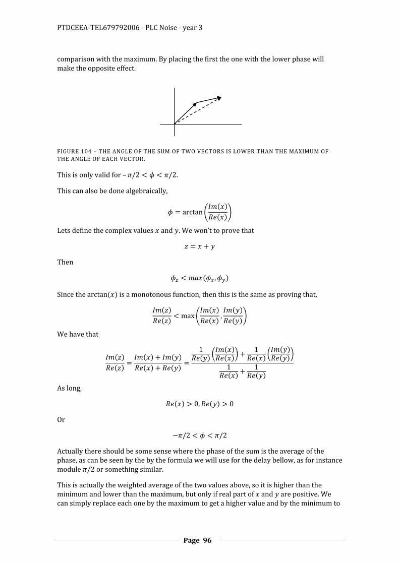
PTDCEEA-TEL679792006 - PLC Noise - year 3
Page 96
comparison with the maximum. By placing the first the one with the lower phase will make the opposite effect.
FIGURE 104 – THE ANGLE OF THE SUM OF TWO VECTORS IS LOWER THAN THE MAXIMUM OF THE ANGLE OF EACH VECTOR.
This is only valid for – .
This can also be done algebraically,
(
)
Lets define the complex values and . We won’t to prove that
Then
Since the is a monotonous function, then this is the same as proving that,
(
)
We have that
(
)
(
)
As long,
Or
Actually there should be some sense where the phase of the sum is the average of the phase, as can be seen by the by the formula we will use for the delay bellow, as for instance module or something similar.
This is actually the weighted average of the two values above, so it is higher than the minimum and lower than the maximum, but only if real part of and are positive. We can simply replace each one by the maximum to get a higher value and by the minimum to
PTDCEEA-TEL679792006 - PLC Noise - year 3
Page 97
get a lower value. Actually we can loosen this condition a bit namely if and | | and | | . However, the weights in the expression above can have norm greater than one. This cannot be easily seen, but we present an example bellow. One may think that the norm would be greater than one if the denominator goes to zero, but this is not true because the numerator also goes to zero, one has,
(
(
))
| || | | |
| |
As | | | | the result will be ( ) , dependent of the direction, and not
infinity.
The derivative of the phase can also be calculated from,
| | | |
| |
Were, the dot represents the dot product of the vectors associated with the complex numbers. Of course, the phase is in radians.
Examples
Also the question may arise, that for which signals is the phase variation maximum? This can be answered if we think of the Z transform of . Zeros close to the unit circle has very high group delay at that frequency. For instance the signal
will have group delay close to for a small.
Successive of zeros close to the unit circle will result in very high group delay; the impulse response of this will resemble a deformed Gaussian.
Here are two signal that result in phase variations close to . One is the signal
an impulse at the left of the vector. And the other an sinusoidal signal,
Resulting in
That you can check that has phase variation is bellow 2 but close.
One can also see that the phase variation is always negative because our signal is zero for negative time (is causal) . This implies that the group delay is always positive and the phase variation is negative.
PTDCEEA-TEL679792006 - PLC Noise - year 3
Page 98
ESTIMATION OF THE CORRELATION COEFFICIENTS MATRIX OF THE COMPENSATED OFDM SIGNAL VERSION TWO
Since, we are actually trying reduce noise in the receiver by using the correlation between different OFDM carriers, then a better idea than the one we used before may be to determine the impulse position, given by , as the value for , that maximizes the correlation between carriers. So one would like to determine a function that given the measured signal, , gives , so that
| |
With
For all This corresponds to estimating the impulse position.
The correlation will depend on . One might try to minimize the total noise volume, given by the determinant of | |,
| |
This is related to the total capacity of the system after diagonalization of the autocorrelation matrix, although not exactly the same. The capacity given through the diagonalization of , could be achieved if preprocessing in the emitter so that each element in the diagonal would correspond to independent channels, however this would require prior knowledge of the impulse position. This can still be a indicator of expected performance.
Another approach would be to minimize the distance between OFDM carriers received signal complex amplitude, , we will in fact use this approach and show that the two
are related.
We are then interested in minimizing,
∑| |
Resulting in,
∑| |
| |
Removing the terms that do not depend on , noting the sum of one term with its conjugate, one has, that one wishes to minimize,
∑ (
)
Or

PTDCEEA-TEL679792006 - PLC Noise - year 3
Page 99
( ( ∑
)) (d1)
Resulting in
(∑
) (pos2)
Were we should chose the angle so that it is always a positive number (add if it is below zero). To calculate the angle we can use a function that gives the angles given the coordinates of the vector, and , us usually known as .
This corresponds to a sort of average of the phase differences, as saw before. However in the previous discussion we said that this would only be correct for phase between 0 and . In fact looking at the formula (d1) we know that if we consider only the phase of the two points then there will always be two values of that solve the equation: and . This ambiguity cannot be solved by using only two points, but it can be solved if we add a third point. Since we are solving the equation for all the set of points then the ambiguity will be solved.
We can see that minimizing the distance will correspond to maximizing the real part of the correlation. We can see know the relation of the formula with the discussion above. Since we are in fact trying to make the point close in the complex plane, this will corresponded to have a correlation coefficient close to one, which corresponds to maximizing the real part of the correlation. That is
∑
Note that, the absolute value is not required, since, we trying to get the correlation coefficient close to one, which is positive. Negative correlations are not of desired in this case. More accurately, that seems that is the only think we can do, so the results should be similar if we try to maximizing the norm.
Note that we are not using the usual optimal estimator for , that minimizes
*( ) | +, resulting in | .
Taking the expectation operator is equivalent to do ensemble average through several experiments, or random variable samples, so if is the experiment number and is the number of experiments, then, we wish to maximize,
∑
∑
And we are going to get a different for each random variable sample or OFDM symbol, that is , resulting in,
(
∑
∑
)

PTDCEEA-TEL679792006 - PLC Noise - year 3
Page 100
And we wish to determine the value of each , that maximizes this function. Making the derivative to and solving results, as before, in,
(∑
)
Equation (pos2) will maximize the cross-correlation between and , and this should also result in high the cross-correlation between and .
Also note that our actual requirement is not to minimize the differences between the complex amplitude of each carrier, but to minimize the probability of error or minimize the capacity or the noise nD volume, . The bit loading should also be done assuming the noise reduction is done at the receiver so; ideally one would like to maximize the capacity.
We can estimate how the noise volume varies with frequency √ by, calculating the
determinant of a simple two by two matrix (this should be better for capacity calculations since be bit loading will be done individually in each frequency).
√ (
) √
In order to inverse capacity can be achieved not only by reduction the noise, but also by concentrating the noise at certain frequencies (that can be avoided), so one would like to reduce the noise more at the frequencies of higher signal to noise ratio, that is increase the value of the cross-correlation, . However, the formula (pos2) should present good results in most cases.
Still another technique may be to exchange the ensemble average to average through . This can only be done if the quantity we are trying to estimate is constant with . This mean that samples for different values for will be samples from the same distribution and average through k will be equal to ensemble average. Quantities that are more or less independent of will be referred to in the next section.
Using equation (pos2) we have obtained the following results:

PTDCEEA-TEL679792006 - PLC Noise - year 3
Page 101
FIGURE 105 – CORRELATION COEFFICIENTS MATRIX FOR THE NOISE MEASURED WITH TWO AMPLIFIERS ZFL-500+.
FIGURE 106 - CORRELATION COEFFICIENTS MATRIX DIAGONAL FOR THE NOISE MEASURED WITH TWO AMPLIFIERS ZFL-500+. FILE
Bin 1
Bin
2Correlation Coefficients Matrix with one Noise Measured Waveform
500 1000 1500 2000
500
1000
1500
2000
0.1
0.2
0.3
0.4
0.5
0.6
0.7
0.8
0.9
1
0 10 20 30 40 50 60 70 80 90 1000
0.1
0.2
0.3
0.4
0.5
0.6
0.7
0.8
0.9
1
Frequency (MHz)
Corr
ela
tion C
oeff
icie
nt
Correlation Coefficients Matrix Diagonal with one Noise Measured Waveform
Diagonal 1
Diagonal 2
Diagonal 3
Diagonal 4
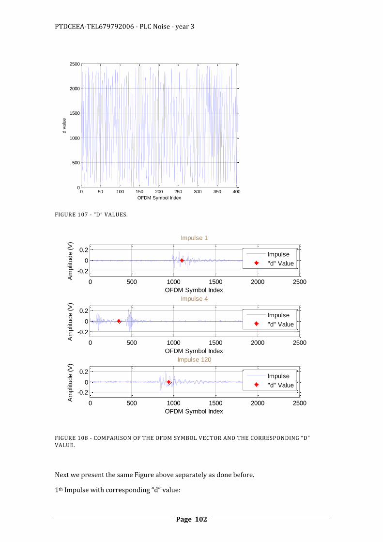
PTDCEEA-TEL679792006 - PLC Noise - year 3
Page 102
FIGURE 107 - “D” VALUES.
FIGURE 108 - COMPARISON OF THE OFDM SYMBOL VECTOR AND THE CORRESPONDING “D” VALUE.
Next we present the same Figure above separately as done before.
1th Impulse with corresponding “d” value:
0 50 100 150 200 250 300 350 4000
500
1000
1500
2000
2500
OFDM Symbol Index
d v
alu
ed values
0 500 1000 1500 2000 2500
-0.2
0
0.2
OFDM Symbol Index
Am
plit
ude (
V)
Impulse 1
0 500 1000 1500 2000 2500
-0.2
0
0.2
OFDM Symbol Index
Am
plit
ude (
V)
Impulse 4
0 500 1000 1500 2000 2500
-0.2
0
0.2
OFDM Symbol Index
Am
plit
ude (
V)
Impulse 120
Impulse
"d" Value
Impulse
"d" Value
Impulse
"d" Value
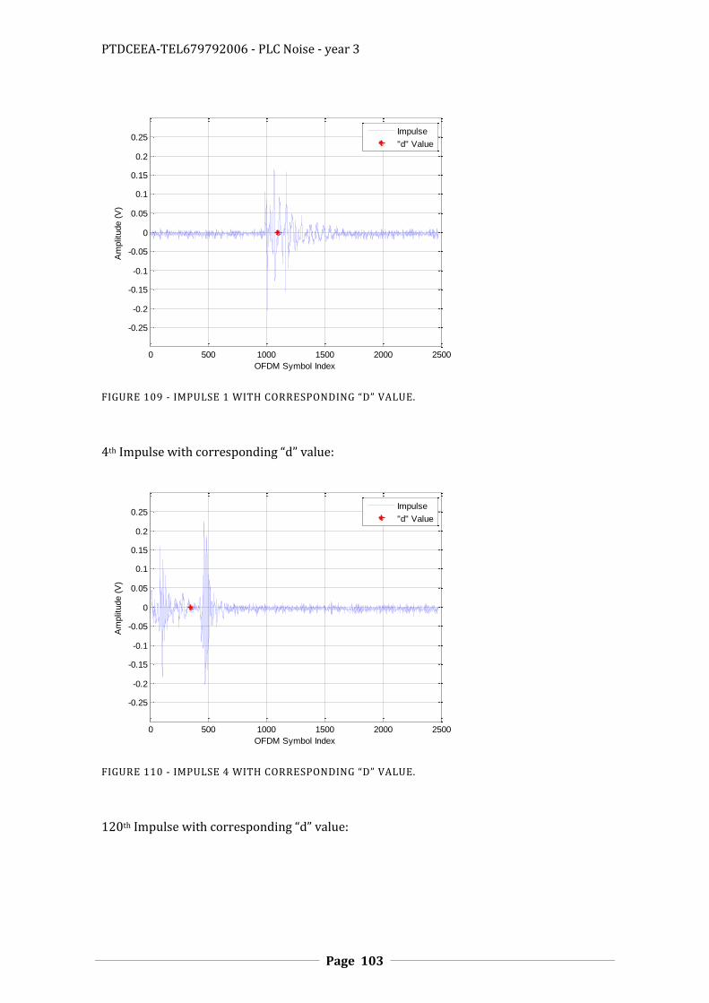
PTDCEEA-TEL679792006 - PLC Noise - year 3
Page 103
FIGURE 109 - IMPULSE 1 WITH CORRESPONDING “D” VALUE.
4th Impulse with corresponding “d” value:
FIGURE 110 - IMPULSE 4 WITH CORRESPONDING “D” VALUE.
120th Impulse with corresponding “d” value:
0 500 1000 1500 2000 2500
-0.25
-0.2
-0.15
-0.1
-0.05
0
0.05
0.1
0.15
0.2
0.25
OFDM Symbol Index
Am
plit
ude (
V)
Impulse 1
Impulse
"d" Value
0 500 1000 1500 2000 2500
-0.25
-0.2
-0.15
-0.1
-0.05
0
0.05
0.1
0.15
0.2
0.25
OFDM Symbol Index
Am
plit
ude (
V)
Impulse 4
Impulse
"d" Value

PTDCEEA-TEL679792006 - PLC Noise - year 3
Page 104
FIGURE 111 - IMPULSE 120 WITH CORRESPONDING “D” VALUE .
FIGURE 112 - COMPARISON OF THE OFDM SYMBOL VECTOR AND THE CORRESPONDING “D” VALUE.
Next we present the same Figure above separately as done before.
2nd Impulse with corresponding “d” value:
0 500 1000 1500 2000 2500
-0.25
-0.2
-0.15
-0.1
-0.05
0
0.05
0.1
0.15
0.2
0.25
OFDM Symbol Index
Am
plit
ude (
V)
Impulse 120
Impulse
"d" Value
0 500 1000 1500 2000 2500
-0.2
0
0.2
OFDM Symbol Index
Am
plit
ude (
V)
Impulse 2
Impulse
"d" Value
0 500 1000 1500 2000 2500
-0.2
0
0.2
OFDM Symbol Index
Am
plit
ude (
V)
Impulse 141
Impulse
"d" Value
0 500 1000 1500 2000 2500
-0.2
0
0.2
OFDM Symbol Index
Am
plit
ude (
V)
Impulse 179
Impulse
"d" Value

PTDCEEA-TEL679792006 - PLC Noise - year 3
Page 105
FIGURE 113 - IMPULSE 2 WITH CORRESPONDING “D” VALUE.
141th Impulse with corresponding “d” value:
FIGURE 114 - IMPULSE 141 WITH CORRESPONDING “D” VALUE .
179th Impulse with corresponding “d” value:
0 500 1000 1500 2000 2500
-0.25
-0.2
-0.15
-0.1
-0.05
0
0.05
0.1
0.15
0.2
0.25
OFDM Symbol Index
Am
plit
ude (
V)
Impulse 2
Impulse
"d" Value
0 500 1000 1500 2000 2500
-0.25
-0.2
-0.15
-0.1
-0.05
0
0.05
0.1
0.15
0.2
0.25
OFDM Symbol Index
Am
plit
ude (
V)
Impulse 141
Impulse
"d" Value

PTDCEEA-TEL679792006 - PLC Noise - year 3
Page 106
FIGURE 115 - IMPULSE 179 WITH CORRESPONDING “D” VALUE.
Comparing the results obtained for the new expression with those obtained above, we can observe that with this new expression the detection of the impulse location is relatively better than the old one. We also observe that for the case where the old expression failed the detection of the impulse position, this new expression also failed in some cases but it’s more closely of the impulse location as we can see for the impulse 147th and also the case of impulse 4th where the new expression failed the detection and the old one don’t.
THE MODEL FOR THE NOISE
One requires a model for the noise after the impulse position compensation, more exactly for the frequency domain autocorrelation matrix .
The main diagonal of the matrix represents the power of the noise signal at each carrier. This is usually estimated during the channel estimation. The next two diagonals are cross correlation between carriers. This should be estimated for each OFDM symbol, and should be high if the symbol as a big impulse or burst noise, and low if the signal has no impulse. Some correlation should always exist even when there are no impulses as long as the noise is not white, but not very high since the DFT approximately diagonalizes a time domain Toeplitz autocorrelation matrix.
In the presence of a burst or impulse, the cross-correlation will be higher. This can happens since the noise will be more or less limited in time, namely at the first time instants after the impulse compensation. Since
A signal limited in time will have Fourier transform with similar properties of the inverse Fourier of a signal limited in frequency. Frequency limited signal can be sampled without loss of information, namely they can be taken as a sum of sinc signals, the same will be
0 500 1000 1500 2000 2500
-0.25
-0.2
-0.15
-0.1
-0.05
0
0.05
0.1
0.15
0.2
0.25
OFDM Symbol Index
Am
plit
ude (
V)
Impulse 2
Impulse
"d" Value

PTDCEEA-TEL679792006 - PLC Noise - year 3
Page 107
true for our signals. If the impulse duration is samples and the symbol duration is , then can only change after more or less units, if the norm of is limited then the variation of in one sample will be limited. This will result in limits for the
cross-correlation,
[( )]
If
| |
In the worst case will be perfectly negatively correlated with , namely,
Resulting in,
[ ] (
)
That is we have a limit for the correlation coefficient. Note that this is if there is no added noise. However the following calculations result in more accurate values.
The proof that the derivative is limited for frequency limited signals namely the norm the inverse Fourier transform and using the Cauchy–Schwarz inequality.
We are trying to calculate the values of the cross-correlation, . The correlation between carriers will be higher if the noise is colored, so this should always be higher than for the white noise case (this could be better explained, it is true for stationary since for white noise is zero). We can progress by writing the expression for each signal in function of the time domain signal,
E U U E * ∑
+
If the signal is white but non-stationary one has, [ ] . The background
noise will not be white, so we should treat this separately, we have
| | |∑
|
So is the Fourier transform of . The noise will be formed by a burst or impulse and
background Gaussian noise. The impulse is moved to the initial time, resulting in slow varying signal, if the burst decreases exponentially then, the Fourier transform will have a pole. It the impulse is rectangular then the Fourier transform will be a sinc. For the case of the background stationary signal, this should be low for greater than zero, but should vary with , so we have,

PTDCEEA-TEL679792006 - PLC Noise - year 3
Page 108
Since for , the two expressions are real and positive we can simple add them, resulting in,
NOISE GENERATION MODEL
An impulsive noise process is stationary. The PDF of the signal is the same, were ever in time we look at it. This is regardless of the fact that impulse appear in some time instants and not in another. Is the impulse position is shift to the origin then it becomes non stationary as previously modeled. A model for impulsive noise is presented bellow for a simple system with no memory. It is simples a random variable with a non-Gaussian PDF, given by the sum of two Gaussians. At each time instant an impulse is generated with probability P, resulting in a Gaussian with a variance of one, or no impulse, a Gaussian with variance of one tenth. The resulting PDF is the sum of the two Gaussians as presented below. (/ImpulseNoise.nb)

PTDCEEA-TEL679792006 - PLC Noise - year 3
Page 109
ESTIMATION OF THE DIFFERENCE BETWEEN THE AUTOCORRELATION AND CROSS-CORRELATION
The difference between Cross-Correlation and Auto Correlation is given by,
| | | |
Using this expression we obtained the following results,

PTDCEEA-TEL679792006 - PLC Noise - year 3
Page 110
FIGURE 109 – DIFFERENCE BETWEEN CROSS-CORRELATION AND AUTO CORRELATION.
THE MODEM
REMOVAL OF SINUSOIDAL SIGNALS
The presence of a sinusoidal signal can be determined at time of channel estimation and simple subtracted by when doing actual transmission.
NOISE TIME CORRELATION FOR DIFFERENT OFDM SYMBOLS
The time correlation of the noise from different OFDM signals is usually because at each frequency bin the noise can usually be taken as white. This is not true if the signal is a sinusoidal signal, but as said before, these signals can be simply subtracted.
ESTIMATING THE CHANNEL TRANSFER FUNCTION SIGNAL TO NOISE RATIO AND INPUT IMPEDANCE
ESTIMATION WITH IMPULSE NOISE
0 50 100 150 200 250 300 350 4000
5
10
15
20
25
30
35
OFDM Symbol Index
dcc v
alu
e
dcc
values
|UC(k)|.|UC(k+1)|-ReUC(k).UC(k+1)*
|UC(k)|.|UC(k+1)|
|UCs(k)|.|UC
s(k+1)|-ReUC
s(k).UC
s(k+1)*

PTDCEEA-TEL679792006 - PLC Noise - year 3
Page 111
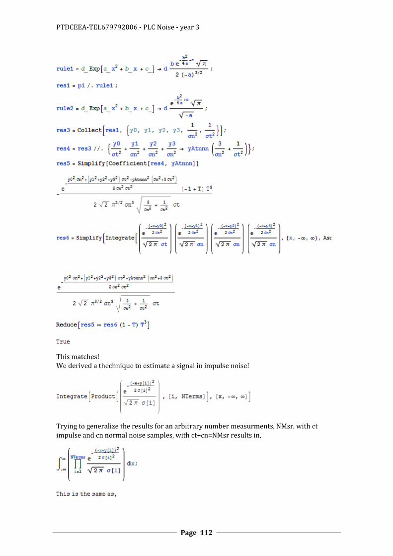
PTDCEEA-TEL679792006 - PLC Noise - year 3
Page 112
This matches! We derived a thechnique to estimate a signal in impulse noise!
Trying to generalize the results for an arbitrary number measurments, NMsr, with ct impulse and cn normal noise samples, with ct+cn=NMsr results in,

PTDCEEA-TEL679792006 - PLC Noise - year 3
Page 113
which is the result bellow
For the denominator
Given a a parameter represented by the random variable X and a set of measurments
represented by the vector random variable Y one wishis to determine the estimate of the sample of X that minimizes the expected square estimation error. This can be represented as:
where y are the measurments, that are samples fo the random variable Y. Minimizing this quantity leads to:
Y represents a set of independent measures with taken from the following distribution.

PTDCEEA-TEL679792006 - PLC Noise - year 3
Page 114
were is gaussian with zero mean and variance and is also gaussian with zero mean
but variance represents an impulse noise in the signal so is large and represents a
normal gaussian noise. This implies that the will have the following distribution, given by a sum of gaussians,
.
Note that conditioned on is gaussian. Represeting and
. The expected value given in equation __ can now be calculated using bayes formula,
if p(x) is constante for the values were p[y|x] is not to low this simplifyes to,
with
were NMsr is the number of measurments. This integral can be calculated directly by expanding all the product terms and using the formulas,
, . However the following method gives a greather insite to the result. Represent the event
that the set of random variables takes a given value as c(j). This values can for example be the the values taken from the binary representation of j with i=0 correponding the the least significant value. We have,

PTDCEEA-TEL679792006 - PLC Noise - year 3
Page 115
and we have,
Representing the values of for c[i] as c[i,j] one has
and
were cn[i] is the the number of zeros in c[i] and ct[i] is the number of ones in c[i].
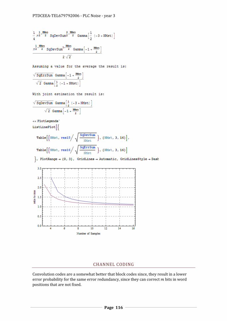
PTDCEEA-TEL679792006 - PLC Noise - year 3
Page 116
CHANNEL CODING
Convolution codes are a somewhat better that block codes since, they result in a lower error probability for the same error redundancy, since they can correct bits in word positions that are not fixed.

PTDCEEA-TEL679792006 - PLC Noise - year 3
Page 117
MAXIMUM CAPACITY USING QAM AND THE CAPACITY OF A BINARY CHANNEL
n – code word length (in symbols)
q=2^b symbols (for binary codes q=2)
a code is forming by selecting
2^k code words
from the possible values.
(n,k) code
Code rate Rc = k / n, corresponds to the decrease of symbol rate due to coding
Redundancy symbols are n - k
At the modulator k symbols are mapped to n symbols
At the demodulator n symbols are mapped to k symbols
Página 437, Digital Communications, Proakis, 4ªed
Bose-Chaudhuri-Hocquenghem (BCH) codes
n=2^m-1
n-k<= mt, m>=3, (in the optimum case we have n-k=2t, so they are not optimum)
d_mim=2t+1
In the table t are the bits the code corrects.
Página 464, Digital Communications, Proakis, 4ªed
Reed-Solomon Codes are a subset of BCH codes. There is not much about the codes. They are non binary and

PTDCEEA-TEL679792006 - PLC Noise - year 3
Page 118
N=q-1=2^k-1
K=1, 2, 3, ..., N-1
Dmin = N-K+1 (they are optimum)
Rc = K/N
k is the number of bits per symbol
Were k (not caps) is the number of bits for a symbol.
Corrects up to
t=1/2 (Dmin-1) = 1/2(N-K)
Symbols (not bits!!!)
There are efficient hard decisions decoding algorithms.
PROBABILITY OF BIT ERROR WITH ERROR CORRECTING
In a word of dimension n, the probability of having t errors or more is, (P(A+B)=P(A)+P(B)-P(A.B)).
(Pe.n)^t (1-Pe)^(n-t) (n*...*(n-t+1)) (Pe.n)^t
As long as Pe.n < 0.1
Reed Solomon codes can correct more than two t errors if the errors are in the same symbol, but only t in the worst case.
The BCH code with n=63, k=45, t=1, g=1701317. How complex is this???
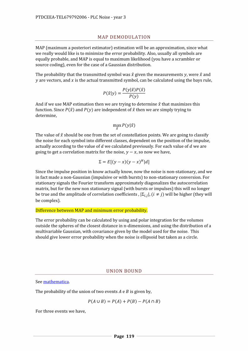
PTDCEEA-TEL679792006 - PLC Noise - year 3
Page 119
MAP DEMODULATION
MAP (maximum a posteriori estimator) estimation will be an approximation, since what we really would like is to minimize the error probability. Also, usually all symbols are equally probable, and MAP is equal to maximum likelihood (you have a scrambler or source coding), even for the case of a Gaussian distribution.
The probability that the transmitted symbol was given the measurements , were and are vectors, and is the actual transmitted symbol, can be calculated using the bays rule,
| |
And if we use MAP estimation then we are trying to determine that maximizes this function. Since and are independent of then we are simply trying to determine,
|
The value of should be one from the set of constellation points. We are going to classify the noise for each symbol into different classes, dependent on the position of the impulse, actually according to the value of we calculated previously. For each value of we are going to get a correlation matrix for the noise, , so now we have,
|
Since the impulse position in know actually know, now the noise is non-stationary, and we in fact made a non-Gaussian (impulsive or with bursts) to non-stationary conversion. For stationary signals the Fourier transform approximately diagonalizes the autocorrelation matrix, but for the new non stationary signal (with bursts or impulses) this will no longer be true and the amplitude of correlation coefficients , | | will be higher (they will
be complex).
Difference between MAP and minimum error probability.
The error probability can be calculated by using and polar integration for the volumes outside the spheres of the closest distance in n-dimensions, and using the distribution of a multivariable Gaussian, with covariance given by the model used for the noise. This should give lower error probability when the noise is ellipsoid but taken as a circle.
UNION BOUND
See mathematica.
The probability of the union of two events e is given by,
For three events we have,

PTDCEEA-TEL679792006 - PLC Noise - year 3
Page 120
In general we can write,
( ) ∑ ∑ ( ) ∑ ( ) ∑ ( )
Were the sums are over all possible combinations of the events, and they go until the final term with all the events.
The probability occurring any of equally probable events is given by,
∑ (
)
(UB.1)
But we can also write a more know formula, that uses disjoint events,
∑ (
)
, and, there is also the formula based on the complement of the event probability, the probability of having one event is the complement of the probability of having none,
We have
This also results in
These formulas help given us a feeling about the result, but one can use the exact formulas when doing computer calculations.
Note that the sum of the terms for greater or equal to alternate between positive and negative, the same sign as the term .
∑ (
)
These are also known as the Bonferroni inequalities. We can put this in another way, the number of cases were you have one or more events from a given set of events is equal to the sum of the cases were you have each of the events minus the duplicates minus two times the triplicates minus three times the quadruplicates etc. It helps thinking of probability as the cardinality of sets and saying it in a natural language. That is,
∑ ∑
Or more generally,

PTDCEEA-TEL679792006 - PLC Noise - year 3
Page 121
( ∑
)
∑
(UB.2)
And we have that, for any ,
Equation (UB.1) can be used to calculate the probability of packets errors and (UB2) for coded word errors, although we cannot get a lower bond on the error probability in this case.
We will have for a code that has a word of bits and that corrects bits, the word error probability will be
(
)
This can also be seen by noting that the probability of having or more errors in bits will be equal to the probability of existing at least one bit, , with a error in n bits and of existing at least one bit, , with a error in n bits and … and existing at least one bit, , with a error in n bits minus the probability that some of the bits are the same. So it is lower than the probability of the union bond to the power of .
The packet error probability with a packet of bits will be given by,
(UB.3)
QUALITY OF SERVICE
NOT SO LOW CAPACITY GAP AND HIGH SIGNAL TO NOISE CASE
In the QAM modulation previous discussed will be easier to analyze is the capacity gap is high, because the probably of bit error will be low, and if the signal to noise is high because the distance between constellation point will be proportional to the noise standard deviation, so will study this case.
In order to the MODEM to work under channel estimation errors and errors, and errors in the model of the channel the transmission rate will have to be lower than for perfect channel knowledge. First the channel estimation errors will be addressed. The actual transmission rate will be the capacity calculated with a lower value for the signal to noise ratio. This is similar for to the result for a simple QAM modulation without coding, previously discussed, were the transmission rate that is equal to the capacity of a channel with the signal to noise divided by the capacity gap, . We will refer to this to the gap in signal to noise ration due to channel estimating errors, , the gap to uncertainty in the channel model due to channel variations of imperfect model, . Coding will allow o get closer to capacity, the coding gain will be, , this can be used to reduce a part of the modulation gap . So the transmission rate will be,

PTDCEEA-TEL679792006 - PLC Noise - year 3
Page 122
(
)
, with,
We will start by discussing the capacity gap to channel model estimation error, , the channel estimation gap. Using the channel estimation gap correspond to using caution when doing bit loading, it could also be called the channel estimation caution margin.
Gap due to Channel Model Estimation Errors
The error probability will be equal to the projected error probability if the estimated noise variance is equal to the actual noise variance. If the actual noise variance is higher than the estimated noise variance then the bit error probability will be higher than the projected value, if the actual noise variance is lower than the estimate then the error probability will be higher. Based on the error probability one can calculate the packet retransmission rate. This should be low; a reasonable value could be to use a value of for instance a packet retransmission for every 100 packets transmitted.
In order to be sure that the probability of error is bellow this error rate every time, one should use a higher value for the standard deviation than the actual value measured, or use a lower value for the bit error probability. One the quotient of the variations will be channel estimation gap. Packet error rate will be given by (UB.3)
And coded bit error rate can be defined as,
In order to get a feeling of what is happening we are looking to approximations to the Gaussian complement cumulative distribution.
Approximating the Complement Cumulative Gaussian Function
One has that the error function is given by,
erfc
√ ∫
, for large x,
erfc √
, and the cumulative Gaussian distribution is,
√ ∫
( ercf (
√ ))
, and,
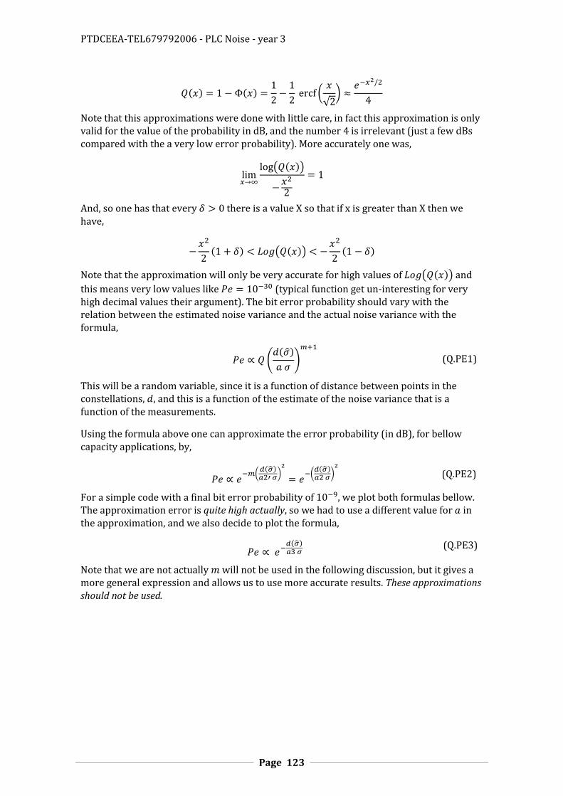
PTDCEEA-TEL679792006 - PLC Noise - year 3
Page 123
ercf (
√ )
Note that this approximations were done with little care, in fact this approximation is only valid for the value of the probability in dB, and the number 4 is irrelevant (just a few dBs compared with the a very low error probability). More accurately one was,
( )
And, so one has that every there is a value X so that if x is greater than X then we have,
( )
Note that the approximation will only be very accurate for high values of ( ) and
this means very low values like (typical function get un-interesting for very high decimal values their argument). The bit error probability should vary with the relation between the estimated noise variance and the actual noise variance with the formula,
(
)
(Q.PE1)
This will be a random variable, since it is a function of distance between points in the constellations, , and this is a function of the estimate of the noise variance that is a function of the measurements.
Using the formula above one can approximate the error probability (in dB), for bellow capacity applications, by,
(
)
(
)
(Q.PE2)
For a simple code with a final bit error probability of , we plot both formulas bellow. The approximation error is quite high actually, so we had to use a different value for in the approximation, and we also decide to plot the formula,
(Q.PE3)
Note that we are not actually will not be used in the following discussion, but it gives a more general expression and allows us to use more accurate results. These approximations should not be used.

PTDCEEA-TEL679792006 - PLC Noise - year 3
Page 124
FIGURE 116- VARIATION OF THE ERROR PROBABILITY WITH THE ACTUAL NOISE VARIANCE. THICK PURPLE IS THE (Q.PE1) THIN BLUE IS (Q.PE2) AND THIN BLACK IS (Q.PE3).
Updating the MAC Gap due to Channel Model Estimation Errors
In an actual implementation the MAC layer could chose channel estimating gap in order to achieve reliable transmission. It we were getting to much packet retransmission due to CRC errors (or the code is correcting too much errors or we could even use an estimate of the actual bit error probability before or after coding) then the channel should be re-estimated and the channel estimating gap increased, corresponding to a decrease in the transmission rate and a decrease in the error probability. If the code isn’t correcting any errors or the likelihoods are high, then the channel estimating gap should be lowered and the transmission rate increased, increasing also the error probability.
How much should the MAC change it and should it increase linearly or exponentially? And what should be its default value? Well if the MODEM is not working ok, then the problem is with the error probability, one should change it a meaningful value. As it can be seen by Figure 116 the error probability is an exponential function of . One can use equation (Q.PE3) to determine the change in to make a change by a factor of in ,
Results in,
That can be approximated by,
(
)
The value for can be the one used for the project error probability. For instance for a
of 2 and a error probability of the resulting change is
(
)
0.8 0.9 1.0 1.1 1.2
10 14
10 12
10 10
10 8P
e

PTDCEEA-TEL679792006 - PLC Noise - year 3
Page 125
Gap due to Channel Model Estimation Errors, Default Value
Let’s consider a MODEM with probability of error (project probability of error close to the uncoded average error probability) with a simple =3 bit error correction code, which needs at least bits of redundancy, with a word of length and with bits packets. The normal retransmission rate (due to CRC errors) of will be one packet in , and channel re-estimation rate of one out of channel estimates? Note, that the packets need to be stored in order to be retransmitted. If the retransmission rate is too high the MAC layer should detect it and estimate the channel again. The probability of packet error is given by (UB3),
(Q.PE)
With is the uncoded bit error rate. So we need to have,
( )
Or
Were we have
( |
)
And is also a random variable since, the measurements are random variables, is the noise standard deviation, a parameter that is assumed to have some real fixed value, since the noise is actually taken to be Gaussian stationary (in this section).
The same symbol will be used for the random variables and their sample or value. If the symbol is used in a place where a random variable should be used then it refers to the random variable, if it is used in a place where a value should be used, then we are referring to the sample.
We have that has a chi-square distribution with degrees of freedom, were is the number of symbols used in the channel estimation and is proportional to . This comes from the bit loading formula, one has,
bits (
)
, and,
√
bits
, resulting in, for high signal to noise,

PTDCEEA-TEL679792006 - PLC Noise - year 3
Page 126
√
√
The density probability of a variable that is a function of another variable is given by,
(
)
( )
Were, is meant to mean to mean | | with very small. This could be used to determine the distribution of , see mathematica.
We will progress in a different way. The error probability can be written as,
(
√∑
)
(
[ √∑
√ ]
)
Were, is normal with zero mean and variance one. Note that the noise variance will cut for this channel estimator. The value of will dictate the average error probability, that, once again we need to determine in order to find the tail of the PDF.
One should try and calculate the variance of . First the variance (using the variance of a chi square distribution) will be , and once again this will cut with the in the denominator, so we have,
(√
)
Were, is Chi-square with N degrees of freedom. Resulting,
And
Were is the projected probability of error used in the bit loading algorithm, and
should be close to average error probability for very large , otherwise the average probability will be significantly higher.
For, , and will results in the project error probability (for perfect channel knowledge) will be but the actual average probability will be
about ten times higher. The resulting probability density is plotted in Figure 117.
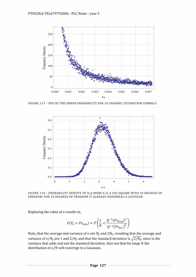
PTDCEEA-TEL679792006 - PLC Noise - year 3
Page 127
FIGURE 117 – PDF OF THE ERROR PROBABILITY FOR 10 CHANNEL ESTIMATION SYMBOLS
FIGURE 118 – PROBABILITY DENSITY OF X/A WERE X IS A CHI-SQUARE WITH 10 DEGREES OF FREEDOM. FOR 10 DEGREES OF FREEDOM IT ALREADY RESEMBLES A GAUSSIAN
Replacing the value of results in,
max (
max
( prj ) )
Note, that the average and variance of are and , resulting that the average and
variance of are 1 and and that the standard deviation is √ , since is the
variance that adds and not the standard deviation. Also not that for large the distribution of will converge to a Gaussian.
0.000 0.001 0.002 0.003 0.004 0.005 0.006 0.007
0
50
100
150
200
250
Pe
Fre
quen
cyD
ensi
ty
0 1 2 3 4 5 6
0.0
0.1
0.2
0.3
0.4
0.5
0.6
x a
Fre
quen
cyD
ensi
ty
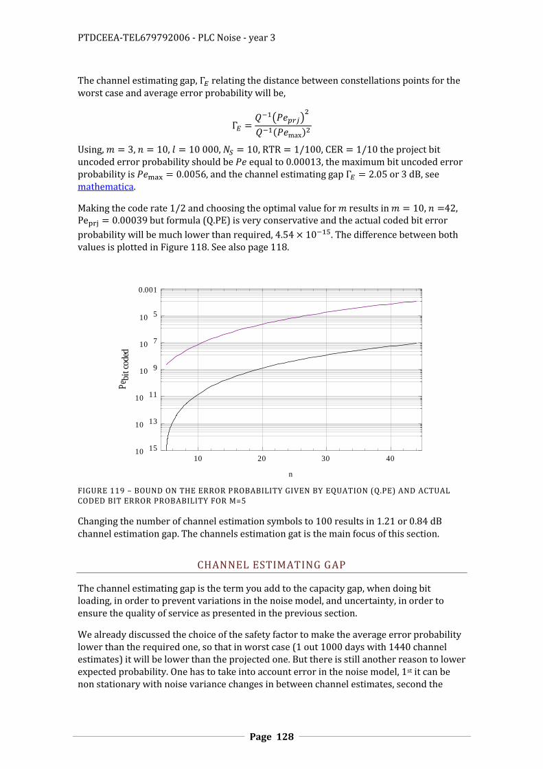
PTDCEEA-TEL679792006 - PLC Noise - year 3
Page 128
The channel estimating gap, relating the distance between constellations points for the worst case and average error probability will be,
( )
max
Using, , , , , , the project bit uncoded error probability should be equal to , the maximum bit uncoded error probability is , and the channel estimating gap or dB, see mathematica.
Making the code rate and choosing the optimal value for results in , 42, but formula (Q.PE) is very conservative and the actual coded bit error
probability will be much lower than required, . The difference between both values is plotted in Figure 118. See also page 118.
FIGURE 119 – BOUND ON THE ERROR PROBABILITY GIVEN BY EQUATION (Q.PE) AND ACTUAL CODED BIT ERROR PROBABILITY FOR M=5
Changing the number of channel estimation symbols to 100 results in 1.21 or 0.84 dB channel estimation gap. The channels estimation gat is the main focus of this section.
CHANNEL ESTIMATING GAP
The channel estimating gap is the term you add to the capacity gap, when doing bit loading, in order to prevent variations in the noise model, and uncertainty, in order to ensure the quality of service as presented in the previous section.
We already discussed the choice of the safety factor to make the average error probability lower than the required one, so that in worst case (1 out 1000 days with 1440 channel estimates) it will be lower than the projected one. But there is still another reason to lower expected probability. One has to take into account error in the noise model, 1st it can be non stationary with noise variance changes in between channel estimates, second the
10 20 30 4010 15
10 13
10 11
10 9
10 7
10 5
0.001
n
Pe b
itco
ded

PTDCEEA-TEL679792006 - PLC Noise - year 3
Page 129
noise may be non Gaussian. This can be handled by further lowering the expected error probability.
However the safety factor can be made adaptive and leave its choice to the MAC layer. This will probably be the best option.
PAM OR NON-ORTHOGONAL CODES PILOTS AND FAST CHANGING CHANNELS
Instead of actually using QAM or PAM to reach capacity, one can also divide each OFDM carrier channel in several different sub-channels using non-orthogonal codes. At the output the signals will add resulting in a higher value signal with several bits as in QAM. The other code in the same channel will appear as noise to each of the other sub-channels so that the capacity in each sub-channel will be close to one. In each sub channel we could use DPSK modulation, so no channel estimation would be required. However, when using DPSK one loses something like of signal to noise ratio, they may allow lowering the safety factor but only in very fast changing channels. Non-orthogonal codes can also be used with channel estimation.
Fast changing channels can be handled with QAM modulation using pilot tones, the number of pilots required would be dependent of the channel impulse response (at the band of interest), namely one would require . This is the same length as
the circular prefix. However note that these pilots could not be all present at a given symbol, but only some in each symbol. Note that if you are close to capacity then it is always required to lose bandwidth to estimate the channel, using pilots is simply acknowledging this, otherwise the signal would be equal to a random signal. Blind channel identification could be possible if the transmission is a bit below capacity, due to a safety factor that may be required, also due to the channel changes for instance, however pilots could also allow reducing the safety factor.
The circular prefix may be used to do blind channels identification and channel state tracking. The value at the circular prefix will be dependent of the previous symbol and the next symbol (there is inter symbol interference in the circular prefix) but both values are known, so you can determine what is the channel. In this case we assume that since we are using PAM or QAM then the signal is somewhat greater than the noise. There is a trend in wireless communications to have the signal close to the noise, to reduce the danger of radiation and save power, but this is not the case in power line communications.
There is still another way to blindly track channel changes: in order to be able to support channel changes the system must be working a bit below capacity. This means that the pdf of the received signal around constellation points will be a bit higher, and this information may be used to track the channel variation. Also if the signal is QAM uniform the rotation of the square can also be used to track channel changes.
Not that is the packets are short as we consider, let’s say about a few OFDM symbols, then channel variation in the packet may not be very important.
THE TECHNIQUES FOR IMPULSIVE OR BURST NOISE REDUCTION
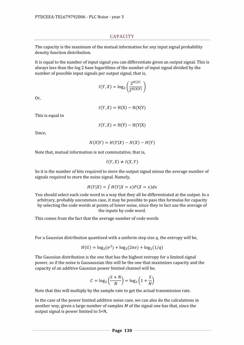
PTDCEEA-TEL679792006 - PLC Noise - year 3
Page 130
CAPACITY
The capacity is the maximum of the mutual information for any input signal probability density function distribution.
It is equal to the number of input signal you can differentiate given an output signal. This is always less than the log 2 base logarithms of the number of input signal divided by the number of possible input signals per output signal, that is,
(
| )
Or,
|
This is equal to
|
Since,
| |
Note that, mutual information is not commutative, that is,
So it is the number of bits required to store the output signal minus the average number of signals required to store the noise signal. Namely,
| ∫ |
You should select each code word in a way that they all be differentiated at the output. In a arbitrary, probably uncommon case, it may be possible to pass this formulas for capacity by selecting the code words at points of lower noise, since they in fact use the average of
the inputs by code word.
This comes from the fact that the average number of code words
For a Gaussian distribution quantized with a uniform step size , the entropy will be,
The Gaussian distribution is the one that has the highest entropy for a limited signal power, so if the noise is Gassaussian this will be the one that maximizes capacity and the capacity of an additive Gaussian power limited channel will be,
(
) (
)
Note that this will multiply by the sample rate to get the actual transmission rate.
In the case of the power limited additive noise case, we can also do the calculations in another way, given a large number of samples of the signal one has that, since the output signal is power limited to S+N,
PTDCEEA-TEL679792006 - PLC Noise - year 3
Page 131
∑
And since the noise signal is also power limited, one has,
∑
This will represent spheres in dimensional case. The capacity will be given by log base 2 of the number of spheres with radios equal to of noise you can place inside a sphere with radios of the signal plus noise. Using the volume of both spheres we will get,
(
)
This is a problem known as sphere packing. The code words will be the center of the spheres. Sphere packing can be improved using different sphere sizes, this may be implemented using nonlinear transformations to the signal in order to get, different noise powers for different input signals. For the low signal to noise case, you cannot place any noise sphere inside the signal plus noise sphere but the capacity is not zero.
In this case you should project assuming is the packed size, and design for a given packet error rate. This will allow intersection between the noise spheres. The error rate should be close to the intersection volume divided by the total volume of the spheres, or maybe to the surface of the noise sphere inside other spheres since the noise variance distribution is not uniform, but one would like to work in the worst case. This should decrease with dimensions for spheres at a fixed distance and constant radios (actually with a constant radio of the distance by the radius). As example consider the case were for working in slow signal to noise the signal is simply repeated N times, resulting with just
two symbols (0,..,0) and (1,…,1). Large noise spheres with radios √ and at distance,
√ , with much smaller than s will overlap greatly, but at high dimension, the overlapping surface, or the surface after the decision plane should be much smaller compared with the sphere surface . (This paragraph needs to be checked). The actual measure will be sphere surfaces with a constant noise variance but then the worst case for the variance must be considered. Higher signal to noise (of course using a lower sampling frequency) can be achieved from low values by using spread spectrum techniques, resulting in another way to reach capacity.
CAPACITY WITH IMPULSIVE NOISE
It was shown that one can use as a model for impulsive noise impulse position dependent OFDM carrier noise covariance matrix, with high non diagonal terms. This means that the covariance of the noise between OFDM carriers will be high for a known impulse position. A high covariance suggest that the noise in each carrier can be reduces by using information from the noise in the other carriers, or in more general terms that the actual amount receiver noise is lower is taken globally that if taken form each carrier individually. This can easily be seen by looking for the formula for the capacity for multi carrier systems. This is,
(
)

PTDCEEA-TEL679792006 - PLC Noise - year 3
Page 132
Were and , are the covariance matrixes of the signal and noise. Using this formula one can find concept of noise volume, , since the determinant is thee volume of the parallelepiped formed by vectors of the columns of hermitian matrix’s, and this will be related to the volume occupied by samples of the noise in the receiver vector space.
High correlation in the noise will result in lower noise volume and higher capacity. Namely, for instance in 2 dimensions a narrow ellipse can be taken as a circle with much greater area if each carrier is taken separately.
This can easily be used to increase the capacity if the covariance matrix is known by the transmitter a priori, but for impulsive noise this is not because it depends on the position of the impulse, that is not known. In the know covariance case, a transformation matrix could be applied at the input that would diagonalizable the noise covariance matrix, allowing to reach capacity, or looking it in another way the noise ellipses could be densely packed in the receiver. This cannot be done if the orientation of the ellipses, namely the impulse position is unknown.
However, at the receiver, a much better noise model will result in better estimation, and lower error rate, and this in turn will allow the transmitter to place some more bits in channel. This will require the receiver to do signal and impulse or impulses position determination.
This may not be easy. Techniques like the ones described before, in estimation with impulse noise could. The likelihood for each model for the noise or impulse position may determine, based on the measurements, and then the final estimation is based on the estimate based on each of the models and the likelihood values. But this may be very computational expensive. Other techniques could be like iterative decoding with soft output likelihood parameters for the signals could be determined for the signal, then the model for the noise could be refined and the likelihood parameters re-estimated. As long as the first estimate is not too bad the refined model for the noise could be used to remove the remaining few errors.
FIGURE 120 – THE INCREASE IN NOISE VOLUME WHEN TAKING CARRIERS INDENPENDENTLY

PTDCEEA-TEL679792006 - PLC Noise - year 3
Page 133
For low signal to noise the impulse position could be determined taking the signal as noise.
How the error probability does decreases with the covariance between carriers and how these affect the bit rate?
CAPACITY FOR NON-GAUSSIAN SIGNALS
Suppose we can transmit n different symbols through the channel and that each symbol can be converted by the noise to symbol with probability, , what is the amount of
information that can be transmitted without errors through the channel?
Another way to look at it is, let’s assume you have a identity channel with noise and that we code (usually just quantify) the transmitted signal using a high number of bits, resulting in a signal that has bits, were is the time, and that you can codify the noise signal (using compression to minimize the number of bits) so that you use bits on the average. Let’s assume also that you can combine in some way (usually adding) the transmitted signal with the noise resulting in the received signal, resulting in the received signal, that is coded (or quantified) in the same way as the transmitted signal with a number of bit equal to , with . Let’s also assume that you let enough time go by, so that the average number of bits is almost equal to the actual number of bits.
Let’s also assume than when you combine the transmitted signal with the noise you will get a received signal that belongs in the set of the possible transmitted signals. This will only be approximately true in practice, since the signals will usually add and the resulting signal will be higher, however you do the adding mod or the adder saturates, then it will be true. We should also assume that when a combining the transmitted signal with two different noises signal the result will be different. This will only be approximately true if the adder saturates. If you can define a subtraction operation that will be the reverse of the combine operation and if for this operation you can also say that for each received signal and any two different noise signals the transmitted signal will be different then you
can say: for each of the possible received signals there are possible transmitted signals and for each of the possible transmitted signals there are possible received signals. Let’s also assume that one of the possible transmitted signals given the received signal is always the received signal, which will correspond to have zero noise. Now we can chose a subset of the transmitted signals that can always be transmitted without error. We first peak one of the transmitted signals, remove from the transmitted signal set all of the possible received signal, then we peak one of the remaining and remove the possible received signals, and so on. Since for each signal we peak we will
remove signals, the number of signals we can choose will be equal to the flour of
.
This implies that the maximum transmission rate through the channel will be equal to .
Note that the noise can always be coded with a lower bit rate that the transmitted signal. This is because you can simply code the noise as a sequence of bits of the same length of the transmitted signal bit sequence, were a one value will correspond to a bit change will a zero value will correspond to no change (and them compress it). A more practical
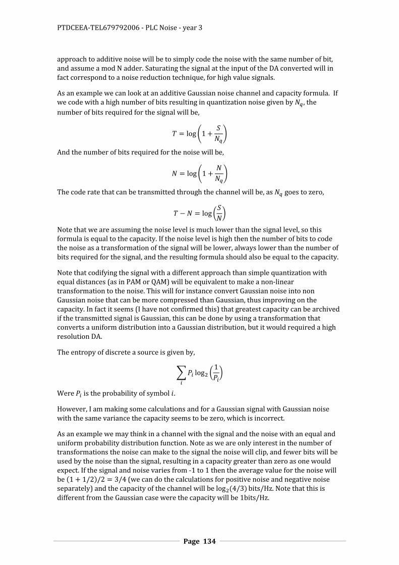
PTDCEEA-TEL679792006 - PLC Noise - year 3
Page 134
approach to additive noise will be to simply code the noise with the same number of bit, and assume a mod N adder. Saturating the signal at the input of the DA converted will in fact correspond to a noise reduction technique, for high value signals.
As an example we can look at an additive Gaussian noise channel and capacity formula. If we code with a high number of bits resulting in quantization noise given by , the
number of bits required for the signal will be,
(
)
And the number of bits required for the noise will be,
(
)
The code rate that can be transmitted through the channel will be, as goes to zero,
(
)
Note that we are assuming the noise level is much lower than the signal level, so this formula is equal to the capacity. If the noise level is high then the number of bits to code the noise as a transformation of the signal will be lower, always lower than the number of bits required for the signal, and the resulting formula should also be equal to the capacity.
Note that codifying the signal with a different approach than simple quantization with equal distances (as in PAM or QAM) will be equivalent to make a non-linear transformation to the noise. This will for instance convert Gaussian noise into non Gaussian noise that can be more compressed than Gaussian, thus improving on the capacity. In fact it seems (I have not confirmed this) that greatest capacity can be archived if the transmitted signal is Gaussian, this can be done by using a transformation that converts a uniform distribution into a Gaussian distribution, but it would required a high resolution DA.
The entropy of discrete a source is given by,
∑
(
)
Were is the probability of symbol .
However, I am making some calculations and for a Gaussian signal with Gaussian noise with the same variance the capacity seems to be zero, which is incorrect.
As an example we may think in a channel with the signal and the noise with an equal and uniform probability distribution function. Note as we are only interest in the number of transformations the noise can make to the signal the noise will clip, and fewer bits will be used by the noise than the signal, resulting in a capacity greater than zero as one would expect. If the signal and noise varies from -1 to 1 then the average value for the noise will be (we can do the calculations for positive noise and negative noise separately) and the capacity of the channel will be . Note that this is different from the Gaussian case were the capacity will be .
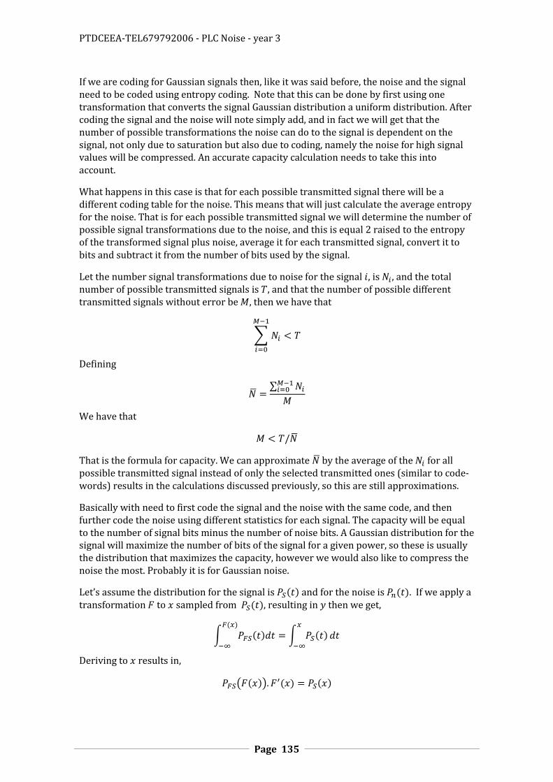
PTDCEEA-TEL679792006 - PLC Noise - year 3
Page 135
If we are coding for Gaussian signals then, like it was said before, the noise and the signal need to be coded using entropy coding. Note that this can be done by first using one transformation that converts the signal Gaussian distribution a uniform distribution. After coding the signal and the noise will note simply add, and in fact we will get that the number of possible transformations the noise can do to the signal is dependent on the signal, not only due to saturation but also due to coding, namely the noise for high signal values will be compressed. An accurate capacity calculation needs to take this into account.
What happens in this case is that for each possible transmitted signal there will be a different coding table for the noise. This means that will just calculate the average entropy for the noise. That is for each possible transmitted signal we will determine the number of possible signal transformations due to the noise, and this is equal 2 raised to the entropy of the transformed signal plus noise, average it for each transmitted signal, convert it to bits and subtract it from the number of bits used by the signal.
Let the number signal transformations due to noise for the signal , is , and the total number of possible transmitted signals is , and that the number of possible different transmitted signals without error be , then we have that
∑
Defining
∑
We have that
That is the formula for capacity. We can approximate by the average of the for all possible transmitted signal instead of only the selected transmitted ones (similar to code-words) results in the calculations discussed previously, so this are still approximations.
Basically with need to first code the signal and the noise with the same code, and then further code the noise using different statistics for each signal. The capacity will be equal to the number of signal bits minus the number of noise bits. A Gaussian distribution for the signal will maximize the number of bits of the signal for a given power, so these is usually the distribution that maximizes the capacity, however we would also like to compress the noise the most. Probably it is for Gaussian noise.
Let’s assume the distribution for the signal is and for the noise is . If we apply a transformation to sampled from , resulting in then we get,
∫
∫
Deriving to results in,
( )
PTDCEEA-TEL679792006 - PLC Noise - year 3
Page 136
So this need to be solved to determine , but further calculations could be done without the actual calculation. For a Gaussian and uniform distribution the solution is known.
An interesting point in this discussion is that the minimum error probability will depend on the code length (the time interval we chose before), even for the best possible code. In fact it may happen that the signal transformation due to noise cannot be coded using the referred number of bits, resulting in an error. However, this error rate number may be very low and the noise is never truly Gaussian. This would be the word error rate. It will go to zero as the code length goes to infinity. It should be correct using automatic repeat request to make it even lower.
This is a theoretical approach to try and understand the channel capacity, but it is not intended for actual implementation. If however, something like that could be done, one should not that the noise would never actually be coded, instead only its coding tables would be determined, in order to chose the set of transmitted signals.
CODES
Coding based of knowledge of all the possible noise transformations, coded as bit sequences that XOR with the signal (see manuscript). Note that there are several possible noise signals for every signal, but that are assuming that this set is the same for every signal.
Let’s assume that there are different signal that will be coded using bits. This will be the word length. The number of different noise signals will be resulting that will be the number of bits required to code all the different noise signals.
Step 1 – Do linear transformation (multiply module 1, that is using XOR’s, by a matrix of zeros and ones) to the noise signal set, so that the new set of , bits noise words will have their initial bits all different, for example they can represent the noise signal index number. The same transformation can be done to the signal.
Step 2 – Start with signal words with the first bits at zero. This will all be transformed code words. To generate the other transformed code words do the following. For each transformed code word and each transformed noise signal generate a new transformed word signal that differs from the original in the bits of the transformed noise word, this can be done simply by a XOR. Since, no sequences of transformed noise can result in zero
THE PROS AND CONS OF ADDING A NEW ESTIMATION PARAMETER
The fact that we do a non linear signal dependent transformation, could imply that one in fact is reducing the amount of information that that can be transmitted, we now have that two different signals may result in two equal signals. However, that is not the case, since we know what the transformation is, and we will invert it when we are trying to estimate the constellation point transmitted. So, different transmitted points in the constellation will still result in different points in the receiver, although different noise signal may result in the same final noise signal.
However, when one estimates the received signal using a determined value for the correlation coefficient at a given symbol, the result may by worse than assuming no
PTDCEEA-TEL679792006 - PLC Noise - year 3
Page 137
correlation if the chosen value is not accurate. So care must be used when using such a technique, as in fact needing to estimate one new parameter, may result in a decrease in performance. However, if the new model is significantly better to represent the noise than the previous one, then much better performance should result.
If one has too many parameters however, using a safe estimation may result in setting all the parameters to zero. In an extreme case we could simply do a non linear transformation, were we would make all the noise constant. However this would require perfect knowledge of the noise, and you can’t have this since it is mixed with the signal. Only a limited amount of information can be extracted about the noise mixed with the signal. I would say that each new one bit parameter you extract from the noise would lower the number of bits you can transmit by one.
If we use the discussion on the next section we can understand what we are doing. We are coding the noise using two parameters, the impulse position and impulse strength, or correlation coefficient angle and amplitude (more parameters can be used), plus normal parameters to code Gaussian noise. This will allow coding the noise using fewer bits, and increase the channel capacity.
DETECTION OF BURST IN SIGNALS
Usually the impulses will be embedded in the signal. In this case what we can do is to determine the impulse position and impulse strength that will result in demodulation with the least errors. So a number of demodulator would run in parallel each for each configuration and the demodulator with least error will be chosen.
However, if the probability of error is low, then we can simply make a first signal estimation without burst reduction, determine an estimate of the noise, and then determine the burst position.
DIVIDING THE SYMBOL LENGTH
When the circular prefix is removed there is a loss of signal level. However, the circular prefix prevents carrier cross-talk noise. If a carrier has a high signal and another as a low signal, this can be a significant part of the noise. So, circular prefix removal is usually required. In order to reduce the loss of signal level due to circular prefix removal, the symbol length should be much higher than the circular prefix.
However, one would like shorts signal to deal with impulses, or burst, if an impulse or burst has a length close to the symbol length, then, is can simply be discarded through forward error correction. One way to solve this would be to prior the typical OFDM coding join N carrier and convert it to time domain, so that in fact the symbol will be divided in N sub symbols with equal, in sequence in time.
A simper way of removing impulses will be to reduce the symbol length by combining two or more carriers, to two or more time domains signals. This will divide the symbol length, in two sub symbols while maintaining the original symbol long to reduce the penalty of the circular prefix. Then using coding the time slots with impulses can be discarded.
CAREFUL CORRELATION ESTIMATION
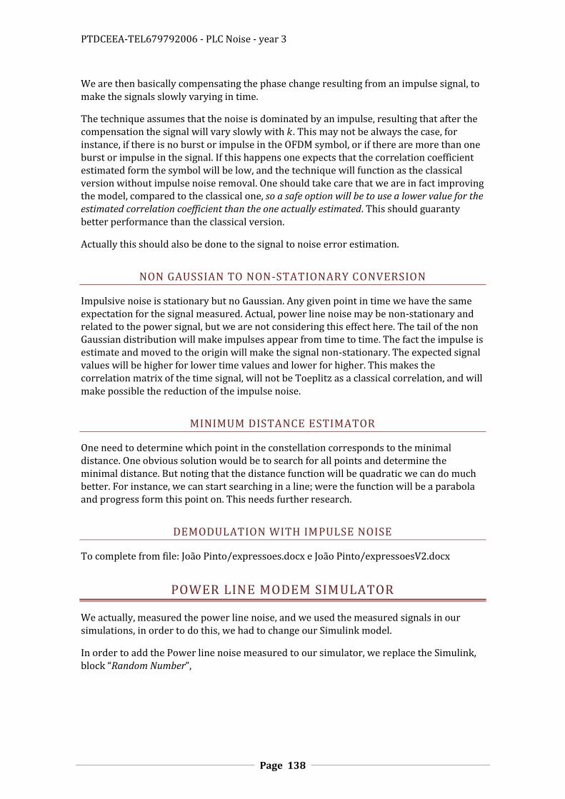
PTDCEEA-TEL679792006 - PLC Noise - year 3
Page 138
We are then basically compensating the phase change resulting from an impulse signal, to make the signals slowly varying in time.
The technique assumes that the noise is dominated by an impulse, resulting that after the compensation the signal will vary slowly with . This may not be always the case, for instance, if there is no burst or impulse in the OFDM symbol, or if there are more than one burst or impulse in the signal. If this happens one expects that the correlation coefficient estimated form the symbol will be low, and the technique will function as the classical version without impulse noise removal. One should take care that we are in fact improving the model, compared to the classical one, so a safe option will be to use a lower value for the estimated correlation coefficient than the one actually estimated. This should guaranty better performance than the classical version.
Actually this should also be done to the signal to noise error estimation.
NON GAUSSIAN TO NON-STATIONARY CONVERSION
Impulsive noise is stationary but no Gaussian. Any given point in time we have the same expectation for the signal measured. Actual, power line noise may be non-stationary and related to the power signal, but we are not considering this effect here. The tail of the non Gaussian distribution will make impulses appear from time to time. The fact the impulse is estimate and moved to the origin will make the signal non-stationary. The expected signal values will be higher for lower time values and lower for higher. This makes the correlation matrix of the time signal, will not be Toeplitz as a classical correlation, and will make possible the reduction of the impulse noise.
MINIMUM DISTANCE ESTIMATOR
One need to determine which point in the constellation corresponds to the minimal distance. One obvious solution would be to search for all points and determine the minimal distance. But noting that the distance function will be quadratic we can do much better. For instance, we can start searching in a line; were the function will be a parabola and progress form this point on. This needs further research.
DEMODULATION WITH IMPULSE NOISE
To complete from file: João Pinto/expressoes.docx e João Pinto/expressoesV2.docx
POWER LINE MODEM SIMULATOR
We actually, measured the power line noise, and we used the measured signals in our simulations, in order to do this, we had to change our Simulink model.
In order to add the Power line noise measured to our simulator, we replace the Simulink, block “Random Number”,
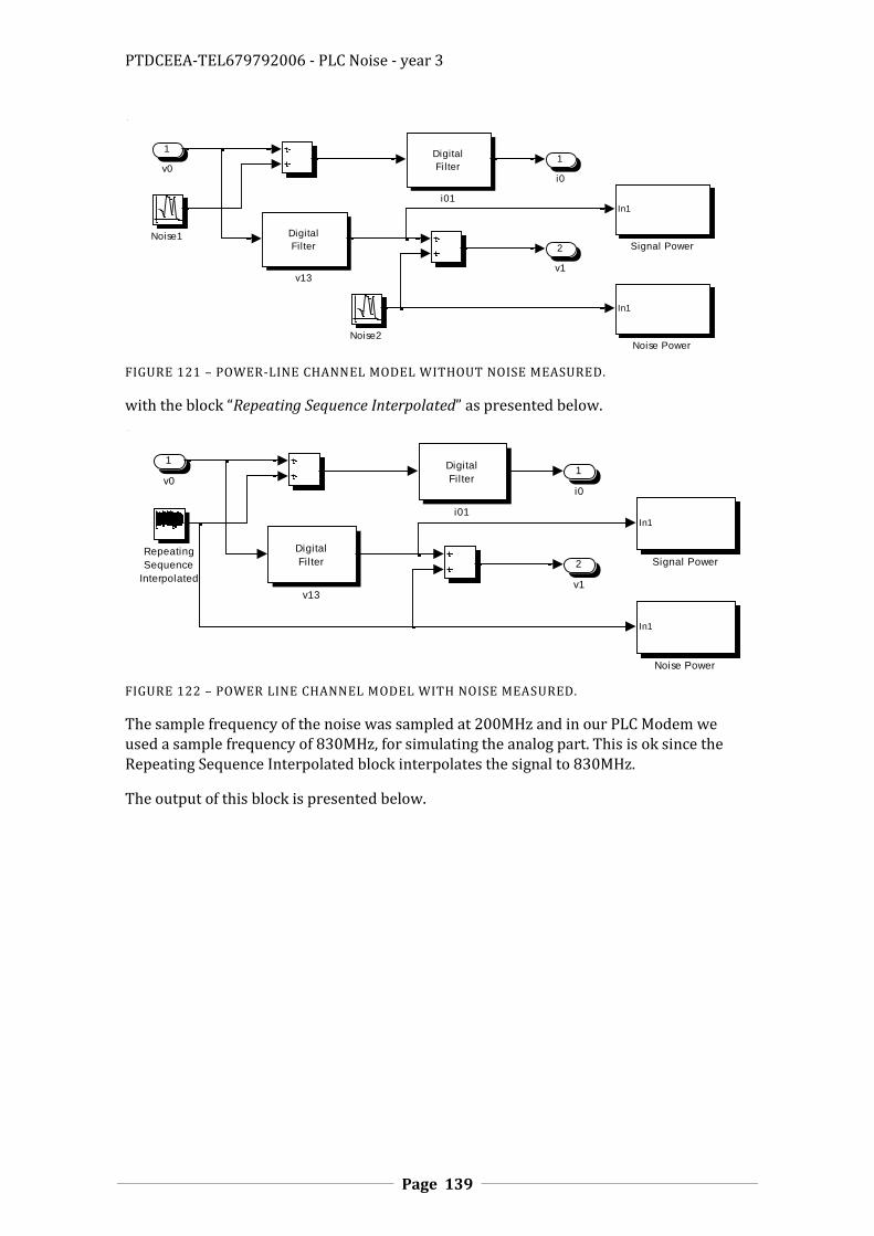
PTDCEEA-TEL679792006 - PLC Noise - year 3
Page 139
FIGURE 121 – POWER-LINE CHANNEL MODEL WITHOUT NOISE MEASURED.
with the block “Repeating Sequence Interpolated” as presented below.
FIGURE 122 – POWER LINE CHANNEL MODEL WITH NOISE MEASURED.
The sample frequency of the noise was sampled at 200MHz and in our PLC Modem we used a sample frequency of 830MHz, for simulating the analog part. This is ok since the Repeating Sequence Interpolated block interpolates the signal to 830MHz.
The output of this block is presented below.
2
v1
1
i0
Digital
Filter
v13
Digital
Filter
i01In1
Signal Power
Noise2
Noise1
In1
Noise Power
1
v0
2
v1
1
i0
Digital
Filter
v13
Digital
Filter
i01In1
Signal PowerRepeating
Sequence
Interpolated
In1
Noise Power
1
v0
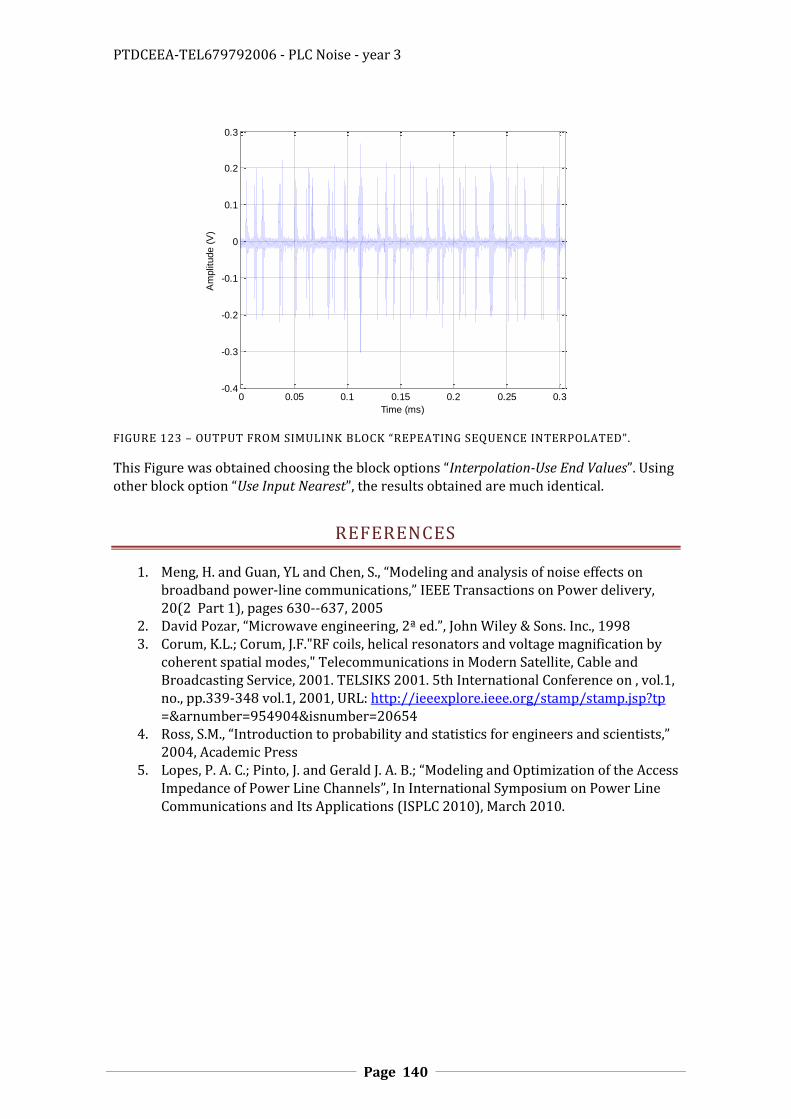
PTDCEEA-TEL679792006 - PLC Noise - year 3
Page 140
FIGURE 123 – OUTPUT FROM SIMULINK BLOCK “REPEATING SEQUENCE INTERPOLATED”.
This Figure was obtained choosing the block options “Interpolation-Use End Values”. Using other block option “Use Input Nearest”, the results obtained are much identical.
REFERENCES
1. Meng, H. and Guan, YL and Chen, S., “Modeling and analysis of noise effects on broadband power-line communications,” IEEE Transactions on Power delivery, 20(2 Part 1), pages 630--637, 2005
2. David Pozar, “Microwave engineering, 2ª ed.”, John Wiley & Sons. Inc., 1998 3. Corum, K.L.; Corum, J.F."RF coils, helical resonators and voltage magnification by
coherent spatial modes," Telecommunications in Modern Satellite, Cable and Broadcasting Service, 2001. TELSIKS 2001. 5th International Conference on , vol.1, no., pp.339-348 vol.1, 2001, URL: http://ieeexplore.ieee.org/stamp/stamp.jsp?tp =&arnumber=954904&isnumber=20654
4. Ross, S.M., “Introduction to probability and statistics for engineers and scientists,” 2004, Academic Press
5. Lopes, P. A. C.; Pinto, J. and Gerald J. A. B.; “Modeling and Optimization of the Access Impedance of Power Line Channels”, In International Symposium on Power Line Communications and Its Applications (ISPLC 2010), March 2010.
0 0.05 0.1 0.15 0.2 0.25 0.3-0.4
-0.3
-0.2
-0.1
0
0.1
0.2
0.3
Am
plit
ude (
V)
Time (ms)
Output of SIMULINK Block "Repeating Sequence Interpolated"