table of contents • index • reviews • reader reviews • errata oracle sql...
TRANSCRIPT
• Table of
Contents
• Index
• Reviews
• Reader
Reviews
• Errata
Oracle SQL Tuning Pocket Reference
By Mark Gurry
Publisher : O'Reilly
Pub Date : January 2002
ISBN : 0-596-00268-8
Pages : 108
Copyright
Chapter 1. Oracle SQL TuningPocket Reference
Section 1.1. Introduction
Section 1.2. The SQL Optimizers
Section 1.3. Rule-Based Optimizer Problems and Solutions
Section 1.4. Cost-Based Optimizer Problems and Solutions
Section 1.5. Problems Common to Rule and Cost with Solutions
Section 1.6. Handy SQL Tuning Tips
Section 1.7. Using SQL Hints
Section 1.8. Using DBMS_STATS to Manage Statistics
Section 1.9. Using Outlines for Consistent Execution Plans
Index

Chapter 1. Oracle SQL TuningPocket Reference
Section 1.1. Introduction
Section 1.2. The SQL Optimizers
Section 1.3. Rule-Based Optimizer Problems and Solutions
Section 1.4. Cost-Based Optimizer Problems and Solutions
Section 1.5. Problems Common to Rule and Cost with Solutions
Section 1.6. Handy SQL Tuning Tips
Section 1.7. Using SQL Hints
Section 1.8. Using DBMS_STATS to Manage Statistics
Section 1.9. Using Outlines for Consistent Execution Plans
1.1 Introduction
This book is a quick-reference guide for tuning Oracle SQL. This is not a comprehensive Oracle
tuning book.
The purpose of this book is to give you some light reading material on my "real world" tuning
experiences and those of my company, Mark Gurry & Associates. We tune many large Oracle sites.
Many of those sites, such as banks, large financial institutions, stock exchanges, and electricity
markets, are incredibly sensitive to poor performance.
With more and more emphasis being placed on 24/7 operation, the pressure to make SQL perform in
production becomes even more critical. When a new SQL statement is introduced, we have to be
absolutely sure that it is going to perform. When a new index is added, we have to be certain that it
will not be used inappropriately by existing SQL statements. This book addresses these issues.
Many sites are now utilizing third-party packages such as Peoplesoft, SAP, Oracle Applications,
Siebel, Keystone, and others. Tuning SQL for these applications must be done without placing hints
on SQL statements, because you are unauthorized to touch the application code. Obviously, for
similar reasons, you can't rewrite the SQL. But don't lose heart; there are many tips and tricks in this
reference that will assist you when tuning packaged software.
This book portrays the message, and my firm belief, that there is always a way of improving your
performance to make it acceptable to your users.
1.1.1 Acknowledgments
Many thanks to my editor, Jonathan Gennick. His feedback and suggestions have added significant
improvements and clarity to this book. A hearty thanks to my team of technical reviewers: Sanjay
Mishra, Stephen Andert, and Tim Gorman.Thanks also to my Mark Gurry & Associates consultants
for their technical feedback. Special thanks to my wife Juliana for tolerating me during yet another
book writing exercise.
1.1.2 Caveats
This book does not cover every type of environment, nor does it cover all performance tuning
scenarios that you will encounter as an Oracle DBA or developer.
I can't stress enough the importance of regular hands-on testing in preparation for being able to
implement your performance tuning recommendations.
1.1.3 Conventions
UPPERCASE
Indicates a SQL keyword
lowercase
Indicates user-defined items such as tablespace names and datafile names Constant width
Used for examples showing code
Constant width bold
Used for emphasis in code examples
[]
Used in syntax descriptions to denote optional elements
{}
Used in syntax descriptions to denote a required choice
|
Used in syntax descriptions to separate choices
1.1.4 What's New in Oracle9i
It's always exciting to get a new release of Oracle. This section briefly lists the new Oracle9i features
that will assist us in getting SQL performance to improve even further than before. The new features
are as follows:
• A new INIT.ORA parameter, FIRST_ROWS_n, that allows the cost-based optimizer to
make even better informed decisions on the optimal execution path for an OLTP application.
The n can equal 1, 10, 100, or 1,000. If you set the parameter to FIRST_ROWS_1, Oracle
will determine the optimum execution path to return one row; FIRST_ROWS_10 will be the
optimum plan to return ten rows; and so on.
• There is a new option called SIMILAR for use with the CURSOR_SHARING parameter.
The advantages of sharing cursors include reduced memory usage, faster parses, and
reduced latch contention. SIMILAR changes literals to bind variables, and differs from the
FORCE option in that similar statements can share the same SQL area without resulting in
degraded execution plans.
• There is a new hint called CURSOR_SHARING_EXACT that allows you to share cursors
for all statements except those with this hint. In essence, this hint turns off cursor sharing for
an individual statement.
• There is a huge improvement in overcoming the skewness problem. The skewness problem
comes about because a bind variable is evaluated after the execution plan is decided. If you
have 1,000,000 rows with STATUS = `C' for Closed, and 100 rows with STATUS = `O' for
Open, Oracle should use the index on STATUS when you query for STATUS = `O', and
should perform a full table scan when you query for STATUS = `C'. If you used bind
variables prior to Oracle9i, Oracle would assume a 50/50 spread for both values, and would
use a full table scan in either case. Oracle 9i determines the value of the bind variable prior
to deciding on the execution plan. Problem solved!
• You can nowidentify unused indexes using the ALTER INDEX MONITOR USAGE
command.
• You can now use DBMS_STATS to gather SYSTEM statistics, including a system's CPU
and I/O usage. You may find that disks are a bottleneck, and Oracle will then have the
information to adjust the execution plans accordingly.
• There are new hints, including NL_AJ, NL_SJ, FACT, NO_FACT, and FIRST_ROWS(n).
All are described in detail in Section 1.7 of this reference.
• Outlines were introduced with Oracle8i to allow you to force execution plans (referred to as
"outlines") for selected SQL statements. However, it was sometimes tricky to force a SQL
statement to use a particular execution path. Oracle9i provides us with the ultimate: we can
now edit the outline using the DBMS_OUTLN_EDIT package.
1.2 The SQL Optimizers
Whenever you execute a SQL statement, a component of the database known as the optimizer must
decide how best to access the data operated on by that statement. Oracle supports two optimizers: the
rule-base optimizer (which was the original), and the cost-based optimizer.
To figure out the optimal execution path for a statement, the optimizers consider the following:
• The syntax you've specified for the statement
• Any conditions that the data must satisfy (the WHERE clauses)
• The database tables your statement will need to access
• All possible indexes that can be used in retrieving data from the table
• The Oracle RDBMS version
• The current optimizer mode
• SQL statement hints
• All available object statistics (generated via the ANALYZE command)
• The physical table location (distributed SQL)
• INIT.ORA settings (parallel query, async I/O, etc.)
Oracle gives you a choice of two optimizing alternatives: the predictable rule-based optimizer and
the more intelligent cost-based optimizer.
1.2.1 Understanding the Rule-Based Optimizer
The rule-based optimizer (RBO) uses a predefined set of precedence rules to figure out which path it
will use to access the database. The RDBMS kernel defaults to the rule-based optimizer under a
number of conditions, including:
• OPTIMIZER_MODE = RULE is specified in your INIT.ORA file
• OPTIMIZER_MODE = CHOOSE is specified in your INIT.ORA file, andno statistics exist
for any table involved in the statement
• An ALTER SESSION SET OPTIMIZER_MODE = RULE command has been issued
• An ALTER SESSION SET OPTIMIZER_MODE = CHOOSEcommand has been issued,
and no statistics exist for any table involved in the statement
• The rule hint (e.g., SELECT /*+ RULE */. . .) has been used in the statement
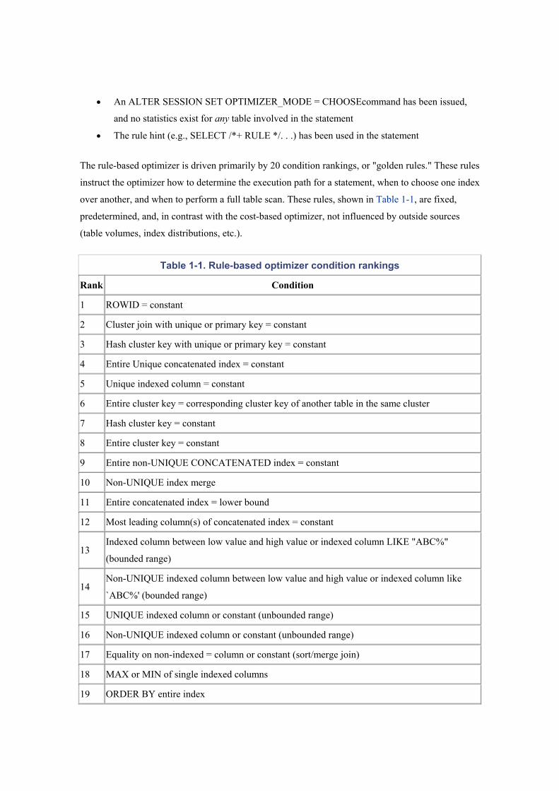
The rule-based optimizer is driven primarily by 20 condition rankings, or "golden rules." These rules
instruct the optimizer how to determine the execution path for a statement, when to choose one index
over another, and when to perform a full table scan. These rules, shown in Table 1-1, are fixed,
predetermined, and, in contrast with the cost-based optimizer, not influenced by outside sources
(table volumes, index distributions, etc.).
Table 1-1. Rule-based optimizer condition rankings
Rank Condition
1 ROWID = constant
2 Cluster join with unique or primary key = constant
3 Hash cluster key with unique or primary key = constant
4 Entire Unique concatenated index = constant
5 Unique indexed column = constant
6 Entire cluster key = corresponding cluster key of another table in the same cluster
7 Hash cluster key = constant
8 Entire cluster key = constant
9 Entire non-UNIQUE CONCATENATED index = constant
10 Non-UNIQUE index merge
11 Entire concatenated index = lower bound
12 Most leading column(s) of concatenated index = constant
13 Indexed column between low value and high value or indexed column LIKE "ABC%"
(bounded range)
14 Non-UNIQUE indexed column between low value and high value or indexed column like
`ABC%' (bounded range)
15 UNIQUE indexed column or constant (unbounded range)
16 Non-UNIQUE indexed column or constant (unbounded range)
17 Equality on non-indexed = column or constant (sort/merge join)
18 MAX or MIN of single indexed columns
19 ORDER BY entire index
20 Full table scans
While knowing the rules is helpful, they alone do not tell you enough about how to tune for the rule-
based optimizer. To overcome this deficiency, the following sections provide some information that
the rules don't tell you.
1.2.1.1 What the RBO rules don't tell you #1
Only single column indexes are ever merged. Consider the following SQL and indexes:
SELECT col1, ...
FROM emp
WHERE emp_name = 'GURRY'
AND emp_no = 127
AND dept_no = 12
Index1 (dept_no)
Index2 (emp_no, emp_name)
The SELECT statement looks at all three indexed columns. Many people believe that Oracle will
merge the two indexes, which involve those three columns, to return the requested data. In fact, only
the two-column index is used; the single-column index is not used. While Oracle will merge two
single-column indexes, it will not merge a multi-column index with another index.
There is one thing to be aware of with respect to this scenario. If the single-column index is a unique
or primary key index, that would cause the single-column index to take precedence over the multi-
column index. Compare rank 4 with rank 9 in Table 1-1.
Oracle8i introduced a new hint, INDEX_JOIN, that allows you to join
multi-column indexes.
1.2.1.2 What the RBO rules don't tell you #2
If all columns in an index are specified in the WHERE clause, that index will be used in preference
to other indexes for which some columns are referenced. For example:
SELECT col1, ...
FROM emp
WHERE emp_name = 'GURRY'
AND emp_no = 127
AND dept_no = 12
Index1 (emp_name)
Index2 (emp_no, dept_no, cost_center)
In this example, only Index1 is used, because the WHERE clause includes all columns for that index,
but does not include all columns for Index2.
1.2.1.3 What the RBO rules don't tell you #3
If multiple indexes can be applied to a WHERE clause, and they all have an equal number of
columns specified, only the index created last will be used. For example:
SELECT col1, ...
FROM emp
WHERE emp_name = 'GURRY'
AND emp_no = 127
AND dept_no = 12
AND emp_category = 'CLERK'
Index1 (emp_name, emp_category) Created 4pm Feb 11th 2002
Index2 (emp_no, dept_no) Created 5pm Feb 11th 2002
In this example, only Index2 is used, because it was created at 5 p.m. and the other index was
created at 4 p.m. This behavior can pose a problem, because if you rebuild indexes in a different
order than they were first created, a different index may suddenly be used for your queries. To deal
with this problem, many sites have a naming standard requiring that indexes are named in
alphabetical order as they are created. Then, if a table is rebuilt, the indexes can be rebuilt in
alphabetical order, preserving the correct creation order. You could, for example, number your
indexes. Each new index added to a table would then be given the next number.
1.2.1.4 What the RBO rules don't tell you #4
If multiple columns of an index are being accessed with an = operator, that will override other
operators such as LIKE or BETWEEN. Two ='s will override two ='s and a LIKE. For example:
SELECT col1, ...
FROM emp
WHERE emp_name LIKE 'GUR%'
AND emp_no = 127
AND dept_no = 12
AND emp_category = 'CLERK'
AND emp_class = 'C1'
Index1 (emp_category, emp_class, emp_name)
Index2 (emp_no, dept_no)
In this example, only Index2 is utilized despite Index1 having three columns accessed and Index2
having only two column accessed.
1.2.1.5 What the RBO rules don't tell you #5
A higher percentage of columns accessed will override a lower percentage of columns accessed. So
generally, the optimizer will choose to use the index from which you specify the highest percentage
of columns. However, as stated previously, all columns specified in a unique or primary key index
will override the use of all other indexes. For example:
SELECT col1, ...
FROM emp
WHERE emp_name = 'GURRY'
AND emp_no = 127
AND emp_class = 'C1'
Index1 (emp_name, emp_class, emp_category)
Index2 (emp_no, dept_no)
In this example, only Index1 is utilized, because 66% of the columns are accessed. Index2 is not
used because a lesser 50% of the indexed columns are used.
1.2.1.6 What the RBO rules don't tell you #6
If you join two tables, the rule-based optimizer needs to select a driving table. The table selected can
have a significant impact on performance, particularly when the optimizer decides to use nested
loops. A row will be returned from the driving table, and then the matching rows selected from the
other table. It is important that as few rows as possible are selected from the driving table.
The rule-based optimizer uses the following rules to select the driving table:
• A unique or primary key index will always cause the associated table to be selected as the
driving table in front of a non-unique or non-primary key index.
• An index for which you apply the equality operator (=) to all columns will take precedence
over indexes from which you use only some columns, and will result in the underlying table
being chosen as the driving table for the query.
• The table that has a higher percentage of columns in an index will override the table that has
a lesser percentage of columns indexed.
• A table that satisfies one two-column index in the WHERE clause of a query will be chosen
as the driving table in front of a table that satisfies two single-column indexes.
• If two tables have the same number of index columns satisfied, the table that is listed last in
the FROM clause will be the driving table. In the SQL below, the EMP table will be the
driving table because it is listed last in the FROM clause.
• SELECT ....
• FROM DEPT d, EMP e
• WHERE e.emp_name = 'GURRY'
• AND d.dept_name = 'FINANCE'
AND d.dept_no = e.dept_no
1.2.1.7 What the RBO rules don't tell you #7
If a WHERE clause has a column that is the leading column on any index, the rule-based optimizer
will use that index. The exception is if a function is placed on the leading index column in the
WHERE clause. For example:
SELECT col1, ...
FROM emp
WHERE emp_name = 'GURRY'
Index1 (emp_name, emp_class, emp_category)
Index2 (emp_class, emp_name, emp_category)
Index1 will be used, because emp_name (used in the WHERE clause) is the leading column. Index2
will not be used, because emp_name is not the leading column.
The following example illustrates what happens when a function is applied to an indexed column:
SELECT col1, ...
FROM emp
WHERE LTRIM(emp_name) = 'GURRY'
In this case, because the LTRIM function has been applied to the column, no index will be used.
1.2.2 Understanding the Cost-Based Optimizer
The cost-based optimizer is a more sophisticated facility than the rule-based optimizer. To determine
the best execution path for a statement, it uses database information such as table size, number of
rows, key spread, and so forth, rather than rigid rules.
The information required by the cost-based optimizer is available once a table has been analyzed via
the ANALYZE command, or via the DBMS_STATS facility. If a table has not been analyzed, the
cost-based optimizer can use only rule-based logic to select the best access path. It is possible to run
a schema with a combination of cost-based and rule-based behavior by having some tables analyzed
and others not analyzed.
The ANALYZE command and the DBMS_STATS functions collect
statistics about tables, clusters, and indexes, and store those statistics in the
data dictionary.
A SQL statement will default to the cost-based optimizer if any one of the tables involved in the
statement has been analyzed. The cost-based optimizer then makes an educated guess as to the best
access path for the other tables based on information in the data dictionary.
The RDBMS kernel defaults to using the cost-based optimizer under a number of situations,
including the following:
• OPTIMIZER_MODE = CHOOSE has been specified in the INIT.ORA file, and statistics
exist for at least one table involved in the statement
• An ALTER SESSION SET OPTIMIZER_MODE = CHOOSE command has been executed,
and statistics exist for at least one table involved in the statement
• An ALTER SESSION SET OPTIMIZER_MODE = FIRST_ROWS (or ALL_ROWS)
command has been executed, and statistics exist for at least one table involved in the
statement
• A statement uses the FIRST_ROWS or ALL_ROWS hint (e.g., SELECT /*+
FIRST_ROWS */. . .)
1.2.2.1 ANALYZE command
The way that you analyze your tables can have a dramatic effect on your SQL performance. If your
DBA forgets to analyze tables or indexes after a table re-build, the impact on performance can be
devastating. If your DBA analyzes each weekend, a new threshold may be reached and Oracle may
change its execution plan. The new plan will more often than not be an improvement, but will
occasionally be worse.
I cannot stress enough that if every SQL statement has been tuned, do not analyze just for the sake of
it. One site that I tuned had a critical SQL statement that returned data in less than a second. The
DBA analyzed each weekend believing that the execution path would continue to improve. One
Monday, morning I got a phone call telling me that the response time had risen to 310 seconds.
If you do want to analyze frequently, use DBMS_STATS.EXPORT_SCHEMA_STATS to back up
the existing statistics prior to re-analyzing. This gives you the ability to revert back to the previous
statistics if things screw up.
When you analyze, you can have Oracle look at all rows in a table (ANALYZE COMPUTE) or at a
sampling of rows (ANALYZE ESTIMATE). Typically, I use ANALYZE ESTIMATE for very large
tables (1,000,000 rows or more), and ANALYZE COMPUTE for small to medium tables.
I strongly recommend that you analyze FOR ALL INDEXED COLUMNS for any table that can
have severe data skewness. For example, if a large percentage of rows in a table has the same value
in a given column, that represents skewness. The FOR ALL INDEXED COLUMNS option makes
the cost-based optimizer aware of the skewness of a column's data in addition to the cardinality
(number-distinct values) of that data.
When a table is analyzed using ANALYZE, all associated indexes are analyzed as well. If an index
is subsequently dropped and recreated, it must be re-analyzed. Be aware that the procedures
DBMS_STATS.GATHER_SCHEMA_STATS and GATHER_TABLE_STATS analyze only tables
by default, not their indexes. When using those procedures, you must specify the
CASCADE=>TRUE option for indexes to be analyzed as well.
Following are some sample ANALYZE statements:
ANALYZE TABLE EMP ESTIMATE STATISTICS SAMPLE 5 PERCENT FOR
ALL INDEXED COLUMNS;
ANALYZE INDEX EMP_NDX1 ESTIMATE STATISTICS SAMPLE 5 PERCENT
FOR ALL INDEXED COLUMNS;
ANALYZE TABLE EMP COMPUTE STATISTICS FOR ALL INDEXED COLUMNS;
If you analyze a table by mistake, you can delete the statistics. For example:
ANALYZE TABLE EMP DELETE STATISTICS;
Analyzing can take an excessive amount of time if you use the COMPUTE option on large objects.
We find that on almost every occasion, ANALYZE ESTIMATE 5 PERCENT on a large table forces
the optimizer make the same decision as ANALYZE COMPUTE.
1.2.2.2 Tuning prior to releasing to production
A major dilemma that exists with respect to the cost-based optimizer (CBO) is how to tune the SQL
for production prior to it being released. Most development and test databases will contain
substantially fewer rows than a production database. It is therefore highly likely that the CBO will
make different decisions on execution plans. Many sites can't afford the cost and inconvenience of
copying the production database into a pre-production database.
Oracle8i and later provides various features to overcome this problem, including DBMS_STATS
and the outline facility. Each is explained in more detail later in this book.
1.2.2.3 Inner workings of the cost-based optimizer
Unlike the rule-based optimizer, the cost-based optimizer does not have hard and fast path
evaluation rules. The cost-based optimizer is flexible and can adapt to its environment. This
adaptation is possible only once the necessary underlying object statistics have been refreshed (re-
analyzed). What is constant is the method by which the cost-based optimizer calculates each possible
execution plan and evaluates its cost (efficiency).
The cost-based optimizer's functionality can be (loosely) broken into the following steps:
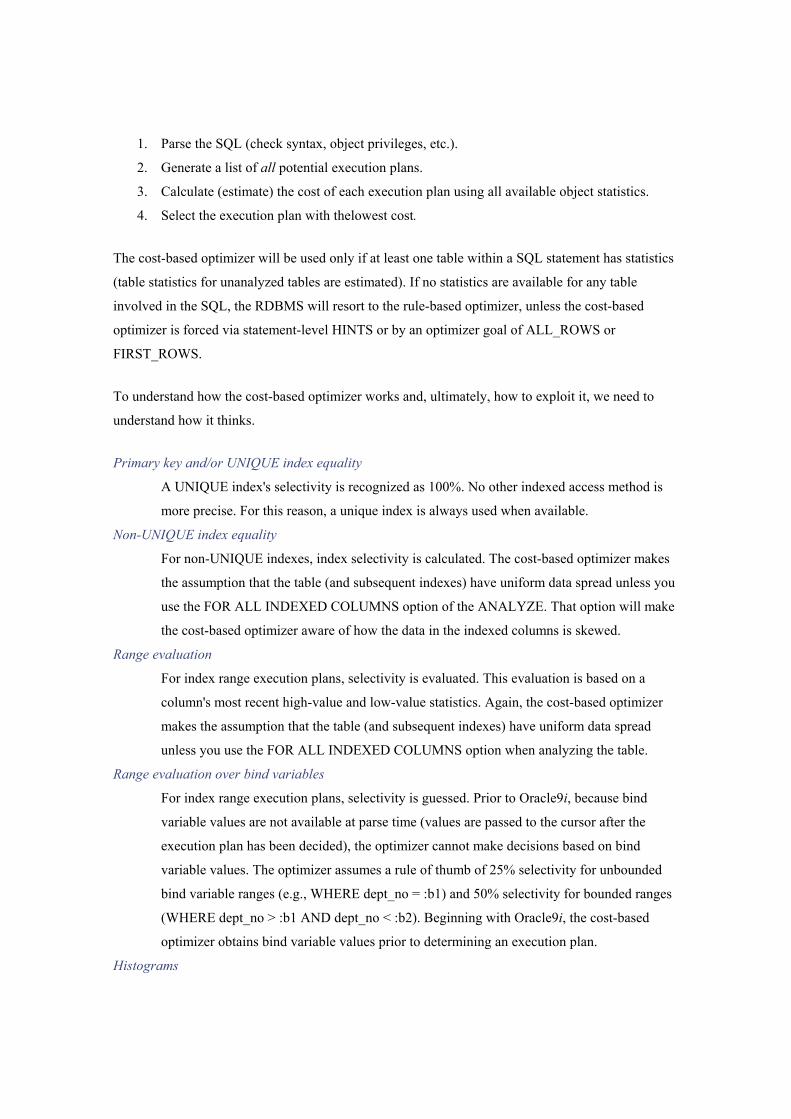
1. Parse the SQL (check syntax, object privileges, etc.).
2. Generate a list of all potential execution plans.
3. Calculate (estimate) the cost of each execution plan using all available object statistics.
4. Select the execution plan with thelowest cost.
The cost-based optimizer will be used only if at least one table within a SQL statement has statistics
(table statistics for unanalyzed tables are estimated). If no statistics are available for any table
involved in the SQL, the RDBMS will resort to the rule-based optimizer, unless the cost-based
optimizer is forced via statement-level HINTS or by an optimizer goal of ALL_ROWS or
FIRST_ROWS.
To understand how the cost-based optimizer works and, ultimately, how to exploit it, we need to
understand how it thinks.
Primary key and/or UNIQUE index equality
A UNIQUE index's selectivity is recognized as 100%. No other indexed access method is
more precise. For this reason, a unique index is always used when available.
Non-UNIQUE index equality
For non-UNIQUE indexes, index selectivity is calculated. The cost-based optimizer makes
the assumption that the table (and subsequent indexes) have uniform data spread unless you
use the FOR ALL INDEXED COLUMNS option of the ANALYZE. That option will make
the cost-based optimizer aware of how the data in the indexed columns is skewed.
Range evaluation
For index range execution plans, selectivity is evaluated. This evaluation is based on a
column's most recent high-value and low-value statistics. Again, the cost-based optimizer
makes the assumption that the table (and subsequent indexes) have uniform data spread
unless you use the FOR ALL INDEXED COLUMNS option when analyzing the table.
Range evaluation over bind variables
For index range execution plans, selectivity is guessed. Prior to Oracle9i, because bind
variable values are not available at parse time (values are passed to the cursor after the
execution plan has been decided), the optimizer cannot make decisions based on bind
variable values. The optimizer assumes a rule of thumb of 25% selectivity for unbounded
bind variable ranges (e.g., WHERE dept_no = :b1) and 50% selectivity for bounded ranges
(WHERE dept_no > :b1 AND dept_no < :b2). Beginning with Oracle9i, the cost-based
optimizer obtains bind variable values prior to determining an execution plan.
Histograms
Prior to the introduction of histograms in Oracle 7.3, The cost-based optimizer could not
distinguish grossly uneven key data spreads.
System resource usage
By default, the cost-based optimizer assumes that you are the only person accessing the
database. Oracle9i gives you the ability to store information about system resource usage,
and can make much better informed decisions based on workload (read up on the
DBMS_STATS.GATHER_SYSTEM_STATS package).
Current statistics are important
The cost-based optimizer can make poor execution plan choices when a table has been
analyzed but its indexes have not been, or when indexes have been analyzed but not the
tables.
You should not force the database to use the cost-based optimizer via inline hints when no
statistics are available for any table involved in the SQL.
Using old (obsolete) statistics can be more dangerous than estimating the statistics at
runtime, but keep in mind that changing statistics frequently can also blow up in your face,
particularly on a mission-critical system with lots of online users. Always back up your
statistics before you re-analyze by using DBMS_STATS.EXPORT_SCHEMA_STATS.
Analyzing large tables and their associated indexes with the COMPUTE option will take a
long, long time, requiring lots of CPU, I/O, and temporary tablespace resources. It is often
overkill. Analyzing with a consistent value, for example, estimate 3%, will usually allow the
cost-based optimizer to make optimal decisions
Combining the information provided by the selectivity rules with other database I/O information
allows the cost-based optimizer to calculate the cost of an execution plan.
1.2.2.4 EXPLAIN PLAN for the cost-based optimizer
Oracle provides information on the cost of query execution via the EXPLAIN PLAN facility.
EXPLAIN PLAN can be used to display the calculated execution cost(s) via some extensions to the
utility. In particular, the plan table's COST column returns a value that increases or decreases to
show the relative cost of a query. For example:
EXPLAIN PLAN FOR
SELECT count(*)
FROM winners, horses
WHERE winners.owner=horses.owner
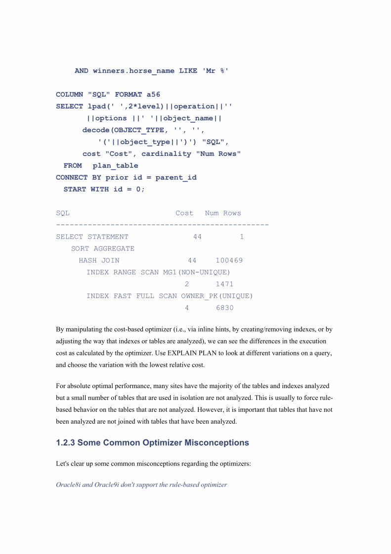
AND winners.horse_name LIKE 'Mr %'
COLUMN "SQL" FORMAT a56
SELECT lpad(' ',2*level)||operation||''
||options ||' '||object_name||
decode(OBJECT_TYPE, '', '',
'('||object_type||')') "SQL",
cost "Cost", cardinality "Num Rows"
FROM plan_table
CONNECT BY prior id = parent_id
START WITH id = 0;
SQL Cost Num Rows
-----------------------------------------------
SELECT STATEMENT 44 1
SORT AGGREGATE
HASH JOIN 44 100469
INDEX RANGE SCAN MG1(NON-UNIQUE)
2 1471
INDEX FAST FULL SCAN OWNER_PK(UNIQUE)
4 6830
By manipulating the cost-based optimizer (i.e., via inline hints, by creating/removing indexes, or by
adjusting the way that indexes or tables are analyzed), we can see the differences in the execution
cost as calculated by the optimizer. Use EXPLAIN PLAN to look at different variations on a query,
and choose the variation with the lowest relative cost.
For absolute optimal performance, many sites have the majority of the tables and indexes analyzed
but a small number of tables that are used in isolation are not analyzed. This is usually to force rule-
based behavior on the tables that are not analyzed. However, it is important that tables that have not
been analyzed are not joined with tables that have been analyzed.
1.2.3 Some Common Optimizer Misconceptions
Let's clear up some common misconceptions regarding the optimizers:
Oracle8i and Oracle9i don't support the rule-based optimizer
This is totally false. Certain publications mentioned this some time ago, but Oracle now
assures us that this is definitely not true.
Hints can't be used with the rule-based optimizer
The large majority of hints can indeed be applied to SQL statements using the rule-based
optimizer.
SQL tuned for rule will run well in cost
If you are very lucky it may, but when you transfer to cost, expect a handful of SQL
statements that require tuning. However, there is not a single site that I have transferred and
been unable to tune.
SQL tuned for cost will run well in rule
This is highly unlikely, unless the code was written with knowledge of the rule-based
optimizer.
You can't run rule and cost together
You can run both together by setting the INIT.ORA parameter OPTIMIZER_MODE to
CHOOSE, and having some tables analyzed and others not. Be careful that you don't join
tables that are analyzed with tables that are not analyzed.
1.2.4 Which Optimizer to Use?
If you are currently using the rule-based optimizer, I strongly recommend that you transfer to the
cost-based optimizer. Here is a list of the reasons why:
• The time spent coding is reduced.
• Coders do not need to be aware of the rules.
• There are more features, and far more tuning tools, available for the cost-based optimizer.
• The chances of third-party packages performing well has been improved considerably.
Many third-party packages are written to run on DB2, Informix, and SQL*Server, as well as
on Oracle. The code has not been written to suit the rule-based optimizer; it has been written
in a generic fashion.
• End users can develop tuned code without having to learn a large set of optimizer rules.
• The cost-based optimizer has improved dramatically from one version of Oracle to the next.
Development of the rule-based optimizer is stalled.
• There is less risk from adding new indexes.
• There are many features that are available only with the cost-based optimizer. These
features include recognition of materialized views, star transformation, the use of function
indexes, and so on. The number of such features is huge, and as time goes on, the gap
between cost and rule will widen.
• Oracle has introduced features such as the DBMS_STATS package and outlines to get
around known problems with the inconsistency of the cost-based optimizer across
environments.
1.3 Rule-Based Optimizer Problems and Solutions
The rule-based optimizer provides a good deal of scope for tuning. Because its behavior is
predictable, and governed by the 20 condition rankings presented earlier in Table 1-1, we are easily
able to manipulate its choices.
I have been tracking the types of problems that occur with both optimizers as well as the best way of
fixing the problems. The major causes of poor rule-based optimizer performance are shown in Table
1-2.
Table 1-2. Common rule-based optimizer problems
Problem % Cases
1. Incorrect driving table 40%
2. Incorrect index 40%
3. Incorrect driving index 10%
4. Using the ORDER BY index and not the WHERE index 10%
Each problem, along with its solution, is explained in detail in the following sections.
1.3.1 Problem 1: Incorrect Driving Table
If the table driving a join is not optimal, there can be a significant increase in the amount of time
required to execute a query. Earlier, in Section 1.2.1.6, I discussed what decides the driving table.
Consider the following example, which illustrates the potential difference in runtimes:
SELECT COUNT(*)
FROM acct a, trans b
WHERE b.cost_center = 'MASS'
AND a.acct_name = 'MGA'
AND a.acct_name = b.acct_name;
In this example, if ACCT_NAME represents a unique key index and COST_CENTER represents a
single column non-unique index, the unique key index would make the ACCT table the driving table.
If both COST_CENTER and ACCT_NAME were single column, non-unique indexes, the rule-
based optimizer would select the TRANS table as the driving table, because it is listed last in the
FROM clause. Having the TRANS table as the driving table would likely mean a longer response
time for a query, because there is usually only one ACCT row for a selected account name but there
are likely to be many transactions for a given cost center.
With the rule-based optimizer, if the index rankings are identical for both tables, Oracle simply
executes the statement in the order in which the tables are parsed. Because the parser processes table
names from right to left, the table name that is specified last (e.g., DEPT in the example above) is
actually the first table processed (the driving table).
SELECT COUNT(*)
FROM acct a, trans b
WHERE b.cost_center = 'MASS'
AND a.acct_name = 'MGA'
AND a.acct_name = b.acct_name;
Response = 19.722 seconds
The response time following the re-ordering of the tables in the FROM clause is as follows:
SELECT COUNT(*)
FROM trans b, acct a
WHERE b.cost_center= 'MASS'
AND a.acct_name = 'MGA'
AND a.acct_name = b.acct_name;
Response = 1.904 seconds
It is important that the table that is listed last in the FROM clause is going to return the fewest
number of rows. There is also potential to adjust your indexing to force the driving table. For
example, you may be able to make the COST_CENTER index a concatenated index, joined with
another column that is frequently used in SQL enquires with the column. This will avoid it ranking
so highly when joins take place.
1.3.2 Problem 2: Incorrect Index
WHERE clauses often provide the rule-based optimizer with a number of indexes that it could utilize.
The rule-based optimizer is totally unaware of how many rows each index will be required to scan
and the potential impact on the response time. A poor index selection will provide a response time
much greater than it would be if a more effective index was selected.
The rule-based optimizer has simple rules for selecting which index to use. These rules and scenarios
are described earlier in the various "What the RBO rules don't tell you" sections.
Let's consider an example.
An ERP package has been developed in a generic fashion to allow a site to use columns for reporting
purposes in any way its users please. There is a column called BUSINESS_UNIT that has a single-
column index on it. Most sites have hundreds of business units. Other sites have only one business
unit.
Our JOURNAL table has an index on (BUSINESS_UNIT), and another on (BUSINESS_UNIT,
ACCOUNT, JOURNAL_DATE). The WHERE clause of a query is as follows:
WHERE business_unit ='A203'
AND account = 801919
AND journal_date between
'01-DEC-2001' and '31-DEC-2001'
The single-column index will be used in preference to the three-column index, despite the fact that
the three-column index returns the result in a fraction of the time of the single-column index. This is
because all columns in the single-column index are used in the query. In such a situation, the only
options open to us are to drop the index or use the cost-based optimizer. If you're not using packaged
software, you may also be able to use hints.
1.3.3 Problem 3: Incorrect Driving Index
The way you specify conditions in the WHERE clause(s) of your SELECT statements has a major
impact on the performance of your SQL, because the order in which you specify conditions impacts
the indexes the optimizer choose to use.
If two index rankings are equal -- for example, two single-column indexes both have their columns
in the WHERE clause -- Oracle will merge the indexes. The merge (AND-EQUAL) order has the
potential to have a significant impact on runtime. If the index that drives the query returns more rows
than the other index, query performance will be suboptimal. The effect is very similar to that from
the ordering of tables in the FROM clause. Consider the following example:
SELECT COUNT(*)
FROM trans
WHERE cost_center = 'MASS'
AND bmark_id = 9;
Response Time = 4.255 seconds
The index that has the column that is listed first in the WHERE CLAUSE will drive the query. In
this statement, the indexed entries for COST_CENTER = `MASS' will return significantly more
rows than those for BMARK_ID=9, which will return at most only one or two rows.
The following query reverses the order of the conditions in the WHERE clause, resulting in a much
faster execution time.
SELECT COUNT(*)
FROM trans
WHERE bmark_id = 9
AND cost_center = 'MASS';
Response Time = 1.044 seconds
For the rule-based optimizer, you should order the conditions that are going to return the fewest
number of rows higher in your WHERE clause.
1.3.4 Problem 4: Using the ORDER BY Indexand not the WHERE Index
A less common problem with index selection, which we have observed at sites using the rule-based
optimizer, is illustrated by the following query and indexes:
SELECT fod_flag, account_no...
FROM account_master
WHERE (account_code like 'I%')
ORDER BY account_no;
Index_1 UNIQUE (ACCOUNT_NO)
Index_2 (ACCOUNT_CODE)
With the indexes shown, the runtime of this query was 20 minutes. The query was used for a report,
which was run by many brokers each day.
In this example, the optimizer is trying to avoid a sort, and has opted for the index that contains the
column in the ORDER BY clause rather than for the index that has the column in the WHERE
clause.
The site that experienced this particular problem was a large stock brokerage. The SQL was run
frequently to produce account financial summaries.
This problem was repaired by creating a concatenated index on both columns:
# Added Index (ACCOUNT_CODE, ACCOUNT_NO)
We decided to drop index_2 (ACCOUNT CODE), which was no longer required because the
ACCOUNT_CODE was the leading column of the new index. The ACCOUNT_NO column was
added to the new index to take advantage of the index storing the data in ascending order. Having
the ACCOUNT_NO column in the index avoided the need to sort, adding the index in a runtime of
under 10 seconds.
1.4 Cost-Based Optimizer Problems and Solutions
The cost-based optimizer has been significantly improved from its initial inception. My
recommendation is that every site that is new to Oracle should be using the cost-based optimizer. I
also recommend that sites currently using the rule-based optimizer have a plan in place for migrating
to the cost-based optimizer. There are, however, some issues with the cost-based optimizer that you
should be aware of. Table 1-3 lists the most common problems I have observed, along with their
frequency of occurrence.
Table 1-3. Common cost-based optimizer problems
Problem % Cases
1. The skewness problem 30%
2. Analyzing with wrong data 25%
3. Mixing the optimizers in joins 20%
4. Choosing an inferior index 20%
5. Joining too many tables < 5%
6. Incorrect INIT.ORA parameter settings < 5%
1.4.1 Problem 1: The Skewness Problem
Imagine that we are consulting at a site with a table TRANS that has a column called STATUS. The
column has two possible values: `O' for Open Transactions that have not been posted, and `C' for
closed transactions that have already been posted and that require no further action. There are over
one million rows that have a status of `C', but only 100 rows that have a status of `O' at any point in
time.
The site has the following SQL statement that runs many hundreds of times daily. The response time
is dismal, and we have been called in to "make it go faster."
SELECT acct_no, customer, product, trans_date, amt
FROM trans
WHERE status='O';
Response time = 16.308 seconds
In this example, taken from a real-life client of mine, the cost-based optimizer decides that Oracle
should perform a full table scan. This is because the cost-based optimizer is aware of how many
distinct values there are for the status column, but is unaware of how many rows exist for each of
those values. Consequently, the optimizer assumes a 50/50 spread of data for each of the two values,
`O' and `C'. Given this assumption, Oracle has decided to perform a full table scan to retrieve open
transactions.
If we inform Oracle of the data skewness by specifying the option FOR ALL INDEXED
COLUMNS when we run the ANALYZE command or when we invoke the DBMS_STATS package,
Oracle will be made aware of the skewness of the data; that is, the number of rows that exist for each
value for each indexed column. In our scenario, the STATUS column is indexed. The following
command is used to analyze the table:
ANALYZE TABLE TRANS COMPUTE STATISTICS
FOR ALL INDEXED COLUMNS
After analyzing the table and computing statistics for all indexed columns, the cost-based optimizer
is aware that there are only 100 or so rows with a status of `O', and it will accordingly use the index
on that column. Use of the index on the STATUS column results in the following, much faster,
query response:
Response Time: 0.259 seconds
Typically the cost-based optimizer will perform a full table scan if the value selected for a column
has over 12% of the rows in the table, and will use the index if the value specified has less than 12%
of the rows. The cost-based optimizer selections are not quite as firm as this, but as a rule of thumb
this is the typical behavior that the cost-based optimizer will follow.
Prior to Oracle9i, if a statement has been written to use bind variables, problems can still occur with
respect to skewness even if you use FOR ALL INDEXED COLUMNS. Consider the following
example:
local_status := 'O';
SELECT acct_no, customer, product, trans_date, amt
FROM trans
WHERE status= local_status;
# Response time = 16.608
Notice that the response time is similar to that experienced when the FOR ALL INDEXED columns
option was not used. The problem here is that the cost-based optimizer isn't aware of the value of the
bind variable when it generates an execution plan. As a general rule, to overcome the skewness
problem, you should do the following:
• Hardcode literals if possible. For example, use WHERE STATUS = `O', not WHERE
STATUS = local_status.
• Always analyze with the option FOR ALL INDEXED COLUMNS.
If you are still experiencing performance problems in which the cost-based optimizer will not use an
index due to bind variables being used, and you can't change the source code, you can try deleting
the statistics off the index using a command such as the following:
ANALYZE INDEX
TRANS_STATUS_NDX
DELETE STATISTICS
Deleting the index statistics works because it forces rule-based optimizer behavior, which will
always use the existing indexes (as opposed to doing full table scans).
Oracle9i will evaluate the bind variable value prior to deciding the execution
plan, obviating the need to hardcode literal values.
1.4.2 Problem 2: Analyzing with Wrong Data
I have been invited to many, many sites that have performance problems at which I quickly
determined that the tables and indexes were not analyzed at a time when they contained typical
volumes of data. The cost-based optimizer requires accurate information, including accurate data
volumes, to have any chance of creating efficient execution plans.
The times when the statistics are most likely to be forgotten or out of date are when a table is rebuilt
or moved, an index is added, or a new environment is created. For example, a DBA might forget to
regenerate statistics after migrating a database schema to a production environment. Other problems
typically occur when the DBA does not have a solid knowledge of the database that he/she is dealing
with and analyzes a table when it has zero rows, instead of when it has hundreds of thousands of
rows shortly afterwards.
1.4.2.1 How to check the last analyzed date
To observe which tables, indexes, and partitions have been analyzed, and when they were last
analyzed, you can select the LAST_ANALYZED column from the various user_XXX view. For
example, to determine the last analyzed date for all your tables:
SELECT table_name, num_rows,
last_analyzed
FROM user_tables;
In addition to user_tables, there are many other views you can select to view the date an object was
last analyzed. To obtain a full list of views with LAST_ANALYZED dates, run the following query:
SELECT table_name
FROM all_tab_columns
WHERE column_name = 'LAST_ANALYZED'
This is not to say that you should be analyzing with the COMPUTE option as often as possible.
Analyzing frequently can cause a tuned SQL statement to become untuned.
1.4.2.2 When to analyze
Re-analyzing tables and indexes can be almost as dangerous as adjusting your indexing, and should
ideally be tested in a copy of the production database prior to being applied to the production
database.
Peoplesoft software is one example of an application that uses temporary holding tables, with the
table names typically ending with _TMP. When batch processing commences, each holding table
will usually have zero rows. As each stage of the batch process completes, insertions and updates are
happening against the holding tables.
The final stages of the batch processing populate the major Peoplesoft transaction tables by
extracting data from the holding tables. When a batch run completes, all rows are usually deleted
from the holding tables. Transactions against the holding tables are not committed until the end of a
batch run, when there are no rows left in the table.
When you run ANALYZE on the temporary holding tables, they will usually have zero rows. When
the cost-based optimizer sees zero rows, it immediately considers full table scans and Cartesian joins.
To overcome this issue, I suggest that you populate the holding tables, and analyze them with data in
them. You can then truncate the tables and commence normal processing. When you truncate a table,
the statistics are not removed.
You can find INSERT and UPDATE SQL statements to use in populating the holding tables by
tracing the batch process that usually populates and updates the tables. You can use the same SQL to
populate the tables.
The runtimes of the batch jobs at one large Peoplesoft site in Australia went from over 36 hours
down to under 30 minutes using this approach.
If analyzing temporary holding tables with production data volumes does not alleviate performance
problems, consider removing the statistics from those tables. This forces SQL statements against the
tables to use rule-based optimizer behavior. You can delete statistics using the ANALYZE TABLE
tname DELETE STATISTICS command. If the statistics are removed, it is important that you not
allow the tables to join with tables that have valid statistics. It is also important that indexes that
have statistics are not used to resolve any queries against the unanalyzed tables. If the temporary
tables are used in isolation, and only joined with each other, the rule-based behavior is often
preferable to that of the cost-based optimizer.
1.4.3 Problem 3: Mixing the Optimizers in Joins
As mentioned in the previous section, when tables are being joined, and one table in the join is
analyzed and the other tables are not, the cost-based optimizer performs at its worst.
When you analyze your tables and indexes using the DBMS_STATS.GATHER_SCHEMA_STATS
procedure and the GATHER_TABLE_STATS procedures, be careful to include the
CASCADE>=TRUE option. By default, the DBMS_STATS package will gather statistics for tables
only. Having statistics on the tables, and not on their indexes, can also cause the cost-based
optimizer to make poor execution plan decisions.
One example of this problem that I experienced recently was at a site that had a TRANS table not
analyzed, and an ACCT table analyzed. The DBA had rebuilt the TRANS table to purge data, and
had simply forgotten to do the analyze afterwards. The following example shows the performance of
a query joining the two tables:
SELECT a.account_name, sum(b.amount)
FROM trans b, acct a
WHERE b.trans_date > sysdate - 7
AND a.acct_id = b.acct_ID
AND a.acct_status = 'A'
GROUP BY account_name;
SORT GROUP BY
NESTED LOOPS
TABLE ACCESS BY ROWID ACCT
INDEX UNIQUE SCAN ACCT_PK
TABLE ACCESS FULL TRANS
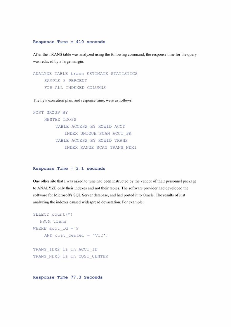
Response Time = 410 seconds
After the TRANS table was analyzed using the following command, the response time for the query
was reduced by a large margin:
ANALYZE TABLE trans ESTIMATE STATISTICS
SAMPLE 3 PERCENT
FOR ALL INDEXED COLUMNS
The new execution plan, and response time, were as follows:
SORT GROUP BY
NESTED LOOPS
TABLE ACCESS BY ROWID ACCT
INDEX UNIQUE SCAN ACCT_PK
TABLE ACCESS BY ROWID TRANS
INDEX RANGE SCAN TRANS_NDX1
Response Time = 3.1 seconds
One other site that I was asked to tune had been instructed by the vendor of their personnel package
to ANALYZE only their indexes and not their tables. The software provider had developed the
software for Microsoft's SQL Server database, and had ported it to Oracle. The results of just
analyzing the indexes caused widespread devastation. For example:
SELECT count(*)
FROM trans
WHERE acct_id = 9
AND cost_center = 'VIC';
TRANS_IDX2 is on ACCT_ID
TRANS_NDX3 is on COST_CENTER
Response Time 77.3 Seconds
Ironically, the software developers were blaming Oracle, claiming that it had inferior performance to
SQL Server. After analyzing the tables and indexes, the response time of this SQL statement was
dramatically improved to 0.415 seconds. The response times for many, many other SQL statements
were also dramatically improved.
The moral of this story could be to let Oracle tuning experts tune Oracle and have SQL Server
experts stick to SQL Server. However, with ever more mobile and cross-database trained IT
professionals, I would suggest that we all take more care in reading the manuals when we tackle the
tuning of a new database.
1.4.4 Problem 4: Choosing an Inferior Index
The cost-based optimizer will sometimes choose an inferior index, despite it appearing obvious that
another index should be used. Consider the following Peoplesoft WHERE clause:
where business_unit = :5
and ledger = :6
and fiscal_year = :7
and accounting_period = :8
and affiliate = :9
and statistics_code = :10
and project_id = :11
and account = :12
and currency_cd = :13
and deptid = :14
and product = :15
The Peoplesoft system from which I took this example had an index that had every single column in
the WHERE clause contained within it. It would seem that Oracle would definitely use that index
when executing the query. Instead, the cost-based optimizer decided to use an index on
(BUSINESS_UNIT, LEDGER, FISCAL_YEAR, ACCOUNT). We extracted the SQL statement and
compared its runtime to that when using a hint to force the use of the larger index. The runtime when
using the index containing all the columns was over four times faster than the runtime obtained when
using the index chosen by the cost-based optimizer.
After further investigation, we observed that the index should have been created as a UNIQUE index,
but had mistakenly been created as a non-UNIQUE index as part of a data purge and table rebuild.
When the index was rebuilt as a unique index, the index was used. The users were obviously happy
with their four-fold performance improvement.
However, more headaches were to come. The same index was the ideal candidate for the following
statement, which was one of the statements run frequently during end-of-month and end-of-year
processing:
where business_unit = :5
and ledger = :6
and fiscal_year = :7
and accounting_period between 1 and 12
and affiliate = :9
and statistics_code = :10
and project_id = :11
and account = :12
and currency_cd = :13
and deptid = :14
and product = :15
Despite the index being correctly created as UNIQUE, the cost-based optimizer was once again
ignoring it. The only difference between this statement and the last is that this statement is after a
range of accounting periods for the financial year rather than just one accounting period.
This WHERE clause used the same incorrect index as previously mentioned, with the columns
(BUSINESS_UNIT, LEDGER, FISCAL_YEAR, and ACCOUNT). Once again, we timed the
statement using the index selected by the cost-based optimizer against the index that contained all of
the columns, and found the larger index to be at least three times faster.
The problem was overcome by repositioning the ACCOUNTING_PERIOD column (originally third
in the index) to be last in the index. The new index order was as follows:
business_unit
ledger
fiscal_year
affiliate
statistics_code
project_id
account
currency_cd
deptid
Product
accounting_period
Another way to force the cost-based optimizer to use an index is to use one of the hints that allows
you to specify an index. This is fine, but often sites are using third-party packages that can't be
modified, and consequently hints can't be utilized. However, there may be the potential to create a
view that contains a hint, with users then accessing the view. A view is useful if the SQL that is
performing badly is from a report or online inquiry that is able to read from views.
As a last resort, I have discovered that sometimes, to force the use of an index, you can delete the
statistics on the index. Occasionally you can also ANALYZE ESTIMATE with just the basic 1,064
rows being analyzed. Often, the execution plan will change to just the way you want it, but this type
of practice is approaching black magic. It is critical that if you adopt such a black magic approach,
you clearly document what you have done to improve performance. Yet another method to try is
lowering the OPTIMIZER_INDEX_COST_ADJ parameter to between 10 and 50.
In summary, why does the cost-based optimizer make such poor decisions? First of all, I must point
out that poor decision-making is the exception rather than the rule. The examples in this section
indicate that columns are looked at individually rather than as a group. If they were looked at as a
group, the cost-based optimizer would have realized in the first example that each row looked at was
unique without the DBA having to rebuild the index as unique. The second example illustrates that if
several of the columns in an index have a low number of distinct values, and the SQL is requesting
most of those values, the cost-based optimizer will often bypass the index. This happens despite the
fact that collectively, the columns are very specific and will return very few rows.
In fairness to the optimizer, queries using indexes with fewer columns will often perform
substantially faster than those using an index with many columns.
1.4.5 Problem 5: Joining Too Many Tables
Early versions of the cost-based optimizer often adopted a divide and conquer approach when more
than five tables were joined. Consider the example shown in Figure 1-1. The query is selecting all
related data for a company whose account ID (in the ACCT_ID column) is equal to 777818. The
company has several branches, and the request is just for the branches in Washington State (WA).
The A table is the ACCT table, the F table is ACCT_ADDRESS, and the G table is the ADDRESS
table.
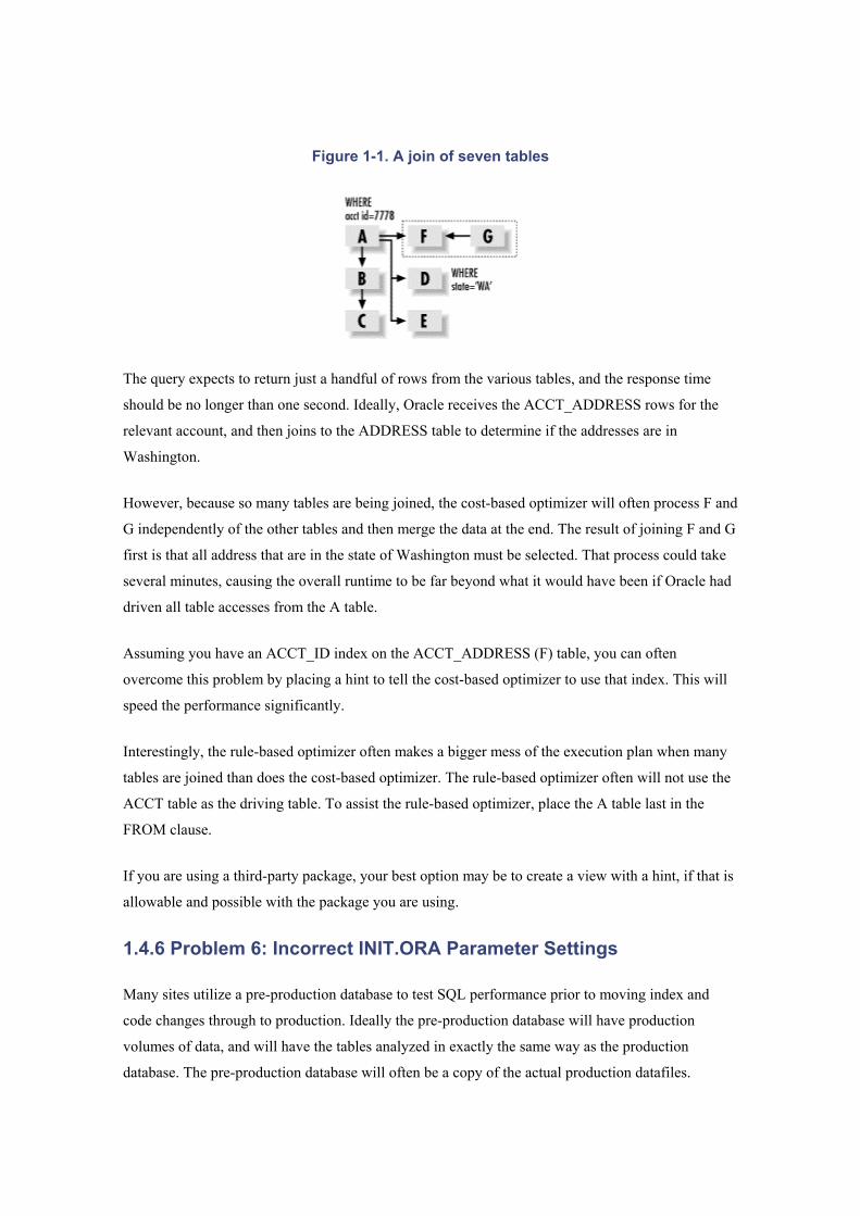
Figure 1-1. A join of seven tables
The query expects to return just a handful of rows from the various tables, and the response time
should be no longer than one second. Ideally, Oracle receives the ACCT_ADDRESS rows for the
relevant account, and then joins to the ADDRESS table to determine if the addresses are in
Washington.
However, because so many tables are being joined, the cost-based optimizer will often process F and
G independently of the other tables and then merge the data at the end. The result of joining F and G
first is that all address that are in the state of Washington must be selected. That process could take
several minutes, causing the overall runtime to be far beyond what it would have been if Oracle had
driven all table accesses from the A table.
Assuming you have an ACCT_ID index on the ACCT_ADDRESS (F) table, you can often
overcome this problem by placing a hint to tell the cost-based optimizer to use that index. This will
speed the performance significantly.
Interestingly, the rule-based optimizer often makes a bigger mess of the execution plan when many
tables are joined than does the cost-based optimizer. The rule-based optimizer often will not use the
ACCT table as the driving table. To assist the rule-based optimizer, place the A table last in the
FROM clause.
If you are using a third-party package, your best option may be to create a view with a hint, if that is
allowable and possible with the package you are using.
1.4.6 Problem 6: Incorrect INIT.ORA Parameter Settings
Many sites utilize a pre-production database to test SQL performance prior to moving index and
code changes through to production. Ideally the pre-production database will have production
volumes of data, and will have the tables analyzed in exactly the same way as the production
database. The pre-production database will often be a copy of the actual production datafiles.
When DBAs test changes in pre-production, they may work fine, but have problems with a different
execution plan being used in production. How can this be? The reason for a different execution plan
in production is often that there are different parameter settings in the production INIT.ORA file
than in the pre-production INIT.ORA file.
I was at one site that ran the following update command and got a four-minute response, despite the
fact that the statement's WHERE clause condition referenced the table's primary key. Oddly, if we
selected from the ACCT table rather than updating it, using the same WHERE clause, the index was
used.
UPDATE acct SET proc_flag = 'Y'
WHERE pkey=100;
# Response Time took 4 minutes and
# wouldn't use the primary key
We tried re-analyzing the table every which way, and eventually removed the statistics. The
statement performed well when the statistics were removed and the rule-based optimizer was used.
After much investigation, we decided to check the INIT.ORA parameters. We discovered that the
COMPATIBLE parameter was set to 8.0.0 despite the database version being Oracle 8.1.7. We
decided to set COMPATIBLE to 8.1.7, and, to our delight, the UPDATE statement correctly used
the index and ran in about 0.1 seconds.
COMPATIBLE is not the only parameter that needs to be set the same in pre-production as in
production to ensure that the cost-based optimizer makes consistent decisions. Other parameters
include the following:
SORT_AREA_SIZE
The number of bytes allocated on a per-user session basis to sort data in memory. If the
parameter is set at its default of 64K, NESTED LOOPS will be favored instead of SORT
MERGES and HASH JOINS.
HASH_AREA_SIZE
The number of bytes to use on a per-user basis to perform hash joins in memory. The
default is twice the SORT_AREA_SIZE. Hash joins often will not work unless this
parameter is set to at least 1 megabyte.
HASH_JOIN_ENABLED
Enables or disables the usage of hash joins. It has a default of TRUE, and usually doesn't
need to be set.
OPTIMIZER_MODE
May be CHOOSE, FIRST_ROWS, or ALL_ROWS. CHOOSE causes the cost-based
optimizer to be used if statistics exist. FIRST_ROWS will operate the same way, but will
tend to favor NESTED LOOPS instead of SORT MERGE or HASH JOINS. ALL_ROWS
will favor SORT MERGEs and HASH JOINS in preference to NESTED LOOP joins.
DB_FILE_MULTIBLOCK_READ_COUNT
The number of blocks that Oracle will retrieve with each read of the table. If you specify a
large value, such as 16 or 32, Oracle will, in many cases, bias towards FULL TABLE
SCANS instead of NESTED LOOPS.
OPTIMIZER_MODE_ENABLE
Enables new optimizer features to be enabled. For example, setting the parameter to 8.1.7
will enable all of the optimizer features up to and including Oracle 8.1.7. This parameter can
also automatically enable other parameters such as FAST_FULL_SCAN_ENABLED.
Some of the major improvements that have occurred with the various Oracle versions
include: 8.0.4 (ordered nested loops, fast full scans), 8.0.5 (many, many optimizer bug fixes),
8.1.6 (improved histograms, partitions, and nested loop processing), 8.1.7 (improved
partition handling and subexpression optimization), and 9.0.1 (much improved index joins,
complex view merging, bitmap improvements, subquery improvements, and push join
predicate improvements).
OPTIMIZER_INDEX_CACHING
Tells Oracle the percentage of index data that is expected to be found in memory. This
parameter defaults to 0, with a range of 0 to 100. The higher the value, the more likely that
NESTED LOOPS will be used in preference to SORT MERGE and HASH JOINs. Some
sites have reported performance improvements when this parameter is set to 90.
OPTIMIZER_INDEX_COST_ADJ
This parameter can be set to encourage the use of indexes. It has a default of 100. If you
lower the parameter to 10, you are telling the cost-based optimizer to lower the cost of index
usage to 10% of its usual value. You can also set the value to something way beyond 100 to
force a SORT MERGE or a HASH JOIN. Sites report performance improvements when the
parameter is set to between 10 and 50 for OLTP and 50 for decision support systems.
Adjusting it downwards may speed up some OLTP enquiries, but make overnight jobs run
forever. If you increase its value, the reverse may occur.
STAR_TRANSFORMATION_ENABLED
Causes a star transformation to be used to combine bitmap indexes on fact table columns.
This is different from the Cartesian join that usually occurs for star queries.
QUERY_REWRITE_ENABLED
Allows the use of function-based indexes as well as allowing query rewrites for materialized
views. The default is FALSE, which may explain why your function indexes are not being
used. Set it to TRUE.
PARTITION_VIEW_ENABLED
Enables the use of partition views. If you are utilizing partitioned views, you will have to set
this parameter to TRUE because the default is FALSE. A partition view is basically a view
that has a UNION ALL join of tables. Partition views were the predecessor to Oracle
partitions, and are used very successfully by many sites for archiving and to speed
performance.
PARALLEL_BROADCAST_ENABLED
This parameter is used by parallel query when small lookup tables are involved. It has a
default of FALSE. If set to TRUE, the rows of small tables are sent to each slave process to
speed MERGE JOIN and HASH JOIN times when joining a small table to a larger table.
OPTIMIZER_MAX_PERMUTATIONS
Can be used to reduce parse times. However, reducing the permutations can cause an
inefficient execution plan, so this parameter should not be modified from its default setting.
CURSOR_SHARING
If set to FORCE or SIMILAR, can result in faster parsing, reduced memory usage in the
shared pool, and reduced latch contention. This is achieved by translating similar statements
that contain literals in the WHERE clause into statements that have bind variables.
The default is EXACT. We suggest that you consider setting this parameter to SIMILAR
with Oracle9i only if you are certain that there are lots of similar statements with the only
differences between them being the values in the literals. It is far better to write your
application to use bind variables if you can.
Setting the parameter to FORCE causes the similar statements to use the same SQL area,
which can degrade performance. FORCE should not be used.
Note that STAR TRANSFORMATION will not work if this parameter is set to SIMILAR
or FORCE.
ALWAYS_SEMI_JOIN
This parameter can make a dramatic improvement to applications that make heavy use of
WHERE EXISTS. Setting this parameter to MERGE or HASH has caused queries to run in
only minutes whereas before they had used up hours of runtime. The default is
STANDARD, which means that the main query (not the subquery) drives the execution plan.
If you specifically set this parameter, the subquery becomes the driving query.
ALWAYS_ANTI_JOIN
This parameter will change the behavior of NOT IN statements, and can speed processing
considerably if set to HASH or MERGE. Setting the parameter causes a merge or hash join
rather than the ugly and time-consuming Cartesian join that will occur with standard NOT
IN execution.
Remember that if any of these parameters are different in your pre-production database than in your
production database, it is possible that the execution plans for your SQL statements will be different.
Make the parameters identical to ensure consistent behavior.
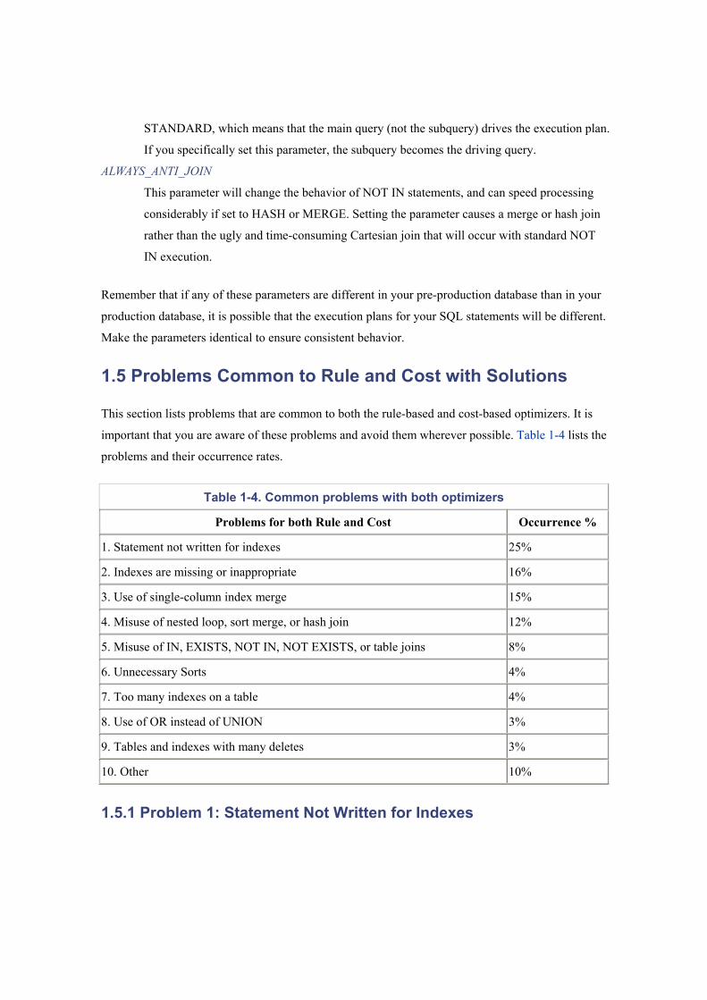
1.5 Problems Common to Rule and Cost with Solutions
This section lists problems that are common to both the rule-based and cost-based optimizers. It is
important that you are aware of these problems and avoid them wherever possible. Table 1-4 lists the
problems and their occurrence rates.
Table 1-4. Common problems with both optimizers
Problems for both Rule and Cost Occurrence %
1. Statement not written for indexes 25%
2. Indexes are missing or inappropriate 16%
3. Use of single-column index merge 15%
4. Misuse of nested loop, sort merge, or hash join 12%
5. Misuse of IN, EXISTS, NOT IN, NOT EXISTS, or table joins 8%
6. Unnecessary Sorts 4%
7. Too many indexes on a table 4%
8. Use of OR instead of UNION 3%
9. Tables and indexes with many deletes 3%
10. Other 10%
1.5.1 Problem 1: Statement Not Written for Indexes
Some SELECT statement WHERE clauses do not use indexes at all. Most such problems are caused
by having a function on an indexed column. Oracle8i and later allow function-based indexes, which
may provide an alternative method of using an effective index.
In the examples in this section, for each clause that cannot use an index, I have suggested an
alternative approach that will allow you to get better performance out of your SQL statements.
In the following example, the SUBSTR function disables the index when it is used over an indexed
column.
Do not use:
SELECT account_name, trans_date, amount
FROM transaction
WHERE SUBSTR(account_name,1,7) = 'CAPITAL';
Use:
SELECT account_name, trans_date, amount
FROM transaction
WHERE account_name LIKE 'CAPITAL%';
In the following example, the!= (not equal) function cannot use an index. Remember that indexes
can tell you what is in a table but not what is not in a table. All references to NOT, !=, and <>
disable index usage.
Do not use:
SELECT account_name,trans_date,amount
FROM transaction
WHERE amount != 0;
Use:
SELECT account_name,trans_date,amount
FROM transaction
WHERE amount > 0 ;
In the following example, the TRUNC function disables the index.
Do not use:
SELECT account_name, trans_date, amount
FROM transaction
WHERE TRUNC(trans_date) = TRUNC(SYSDATE);
Use:
SELECT account_name, trans_date, amount
FROM transaction
WHERE trans_date BETWEEN TRUNC(SYSDATE)
AND TRUNC(SYSDATE) + .99999;
In the following example, || is the concatenate function; it strings two character columns together.
Like other functions, it disables indexes.
Do not use:
SELECT account_name, trans_date, amount
FROM transaction
WHERE account_name || account_type = 'AMEXA';
Use:
SELECT account_name, trans_date, amount
FROM transaction
WHERE account_name ='AMEX'
AND account_type = 'A' ;
In the following example, the addition operator is also a function and disables the index. All the
other arithmetic operators (-, *, and /) have the same effect.
Do not use:
SELECT account_name, trans_date, amount
FROM transaction
WHERE amount + 3000 < 5000;
Use:
SELECT account_name, trans_date, amount
FROM transaction
WHERE amount < 2000;
In the following example, indexes will not be used when a column or columns appears on both sides
of an operator. The result will be a full table scan.
Do not use:
SELECT account_name, trans_date, amount
FROM transaction
WHERE account_name = NVL(:acc_name, account_name);
Use:
SELECT account_name, trans_date, amount
FROM transaction
WHERE account_name LIKE NVL(:acc_name, '%');
As mentioned previously, function indexes can be used if the function in the WHERE clause
represents the same function and column on which the function index was created. For function
indexes to work, you must have the INIT.ORA parameter QUERY_REWRITE_ENABLED set to
TRUE. You must also be using the cost-based analyzer. The statement in the following example uses
a function index:
CREATE INDEX results_fn_ndx1 ON results(UPPER(owner))
SELECT count(*)
FROM results
WHERE UPPER(owner) = 'MR M A GURRY';
Execution Plan
-----------------------------------------
0 SELECT STATEMENT Optimizer=CHOOSE (Cost=1
Card=1 Bytes=32)
1 0 SORT (AGGREGATE)
2 1 INDEX (RANGE SCAN) OF
'RESULTS_FN_NDX1' (NON-UNIQUE)
(Cost=1 Card=1 Bytes=32)
Another common problem that causes indexes not to be used is when the column indexed is one
datatype and the value in the WHERE clause is another data type. Oracle automatically performs a
simple column type conversion, or casting, when it compares two columns of different types.
Assume that EMP_TYPE is an indexed VARCHAR2 column:
SELECT . . .
FROM emp
WHERE emp_type = 123
Execution Plan
-----------------------------------------
SELECT STATEMENT OPTIMIZER HINT: CHOOSE
TABLE ACCESS (FULL) OF 'EMP'
Because EMP_TYPE is a VARCHAR2 value, and the constant 123 is a numeric constant, Oracle
will cast the VARCHAR2 value to a NUMBER value. This statement will actually be processed as:
SELECT . . .
FROM emp
WHERE TO_NUMBER(emp_type) = 123
The EXPLAIN PLAN utility cannot detect or identify casting problems; it simply assumes that all
module bind variables are of the correct type. Programs that are not performing up to expectation
may have a casting problem. The EXPLAIN PLAN output will report that the SQL statement is
correctly using the index, but that won't necessarily be true.
1.5.2 Problem 2: Indexes Are Missing or Inappropriate
While it is important to use indexes to reduce response time, the use of indexes can often actually
lengthen response times considerably. The problem occurs when more than 10% of a table's rows are
accessed using an index.
I am astounded at how many tuners, albeit inexperienced, believe that if a SQL statement uses an
index, it must be tuned. You should always ask, "Is it the best available index?", or "Could an
additional index be added to improve the responsiveness?", or "Would a full table scan produce the
result faster?"
Another important aspect of indexes is that depending on their type and composition, an index can
affect the execution plan of a SQL statement. This must be considered when adding or modifying
indexes.
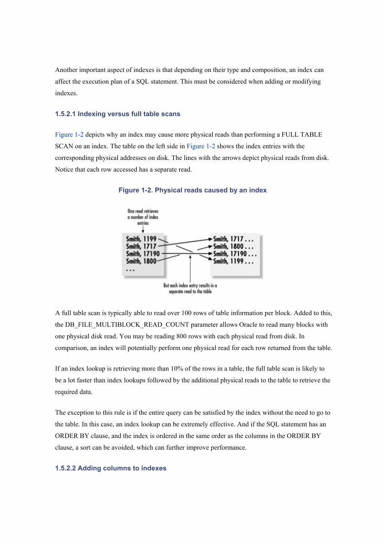
1.5.2.1 Indexing versus full table scans
Figure 1-2 depicts why an index may cause more physical reads than performing a FULL TABLE
SCAN on an index. The table on the left side in Figure 1-2 shows the index entries with the
corresponding physical addresses on disk. The lines with the arrows depict physical reads from disk.
Notice that each row accessed has a separate read.
Figure 1-2. Physical reads caused by an index
A full table scan is typically able to read over 100 rows of table information per block. Added to this,
the DB_FILE_MULTIBLOCK_READ_COUNT parameter allows Oracle to read many blocks with
one physical disk read. You may be reading 800 rows with each physical read from disk. In
comparison, an index will potentially perform one physical read for each row returned from the table.
If an index lookup is retrieving more than 10% of the rows in a table, the full table scan is likely to
be a lot faster than index lookups followed by the additional physical reads to the table to retrieve the
required data.
The exception to this rule is if the entire query can be satisfied by the index without the need to go to
the table. In this case, an index lookup can be extremely effective. And if the SQL statement has an
ORDER BY clause, and the index is ordered in the same order as the columns in the ORDER BY
clause, a sort can be avoided, which can further improve performance.
1.5.2.2 Adding columns to indexes
In the following example, the runtime on the statement was reduced at a large stock brokerage from
40 seconds down to 3 seconds for account_id 100101, which happened to be the largest account in
the table. The response time was critical for answering online customer inquiries. The problem was
solved by adding all of the columns in the WHERE clause, and those in the SELECT list, into the
index. There is the tradeoff that this index now has to be maintained, but the benefits at this site far
outweighed the costs.
SELECT SUM(val)
FROM account_tran
WHERE account_id = 100101
AND fin_yr = '1996'
The original index was on (account_id). The new index was on (account_id, fin_yr, val). The result
was that the index entirely satisfied the query, and the table did not need to be accessed.
Another common problem I notice is that when tables are joined, the leading column of the index is
not the column(s) that the tables are joined on. Consider the following example:
WHERE A.SURNAME = 'GURRY'
AND A.ACCT_NO = T.ACCT_NO
AND T.TRAN_DATE > '01-JUL-97'
AND T.TRAN_TYPE = 'SALARY'
In this situation, many sites will have an index on SURNAME for the ACCT table, and an index on
TRAN_DATE and TRAN_TYPE for the TRANS table. To speed the query significantly, it is best to
add the ACCT_NO join column as the leading column of the TRANS index. What you really want
to have are indexes such as the following:
Index ACCT by (SURNAME)
Index TRANS by (ACCT_NO, TRAN_DATE, TRAN_TYPE)
1.5.2.3 Should I index small tables?
Yet another common problem that I see is small tables that don't have any index at all. I quite often
hear heated debates with one person saying that the index is not required because the table is small
and the data will be stored in memory anyway. They will often explain that the table can even be
created with the cache attribute.
My experience has been that every small table should be indexed. The two reasons for the index are
that the uniqueness of the rows in the table can be enforced by a primary or unique key, and, more
importantly, the optimizer has the opportunity to work out the optimal execution plan for queries
against the table. The example in the following table shows that the response time of a particular
query went from 347 seconds elapsed down to 39.72 seconds elapsed when an index was created on
the table.The most important thing about not having the index is that the optimizer will often create a
less than optimal execution plan without it.
Without index With index
CPU Elapsed CPU Elapsed
PARSE 0.00 0.03 0.01 0.11
EXECUTE 146.14 347.36 18.09 39.60
FETCH 0.00 0.00 0.00 0.00
TOTALS 146.14 347.39 18.10 39.72
1.5.3 Problem 3: Use of Single-Column Index Merge
Early in this reference, I mentioned that Oracle will only join single-column indexes. That is, unless
you use the INDEX_JOIN hint. Single-column index merges are bad news in all relational databases,
not just Oracle. They cause each index entry to be read for the designated value on both indexes.
Consider the following example, which is based on a schema used by a well-known stock brokerage:
INDEX1(APPROVE_FLAG) column and
INDEX2(ADVISOR_CODE)
SELECT COUNT(*)
FROM account_master
WHERE approve_flag='Y'
AND adviser_code='IAM';
3.509 secs
The number of ACCOUNT_MASTER rows that have APPROVE_FLAG = `Y' is around one
million. Oracle reads all of the Y's, and then reads the much lower number of ADIVISOR_CODE =
`IAM' rows, then crunches the results together. By the way, there is a much lower number of N's.
The good news is that Oracle has an easy way around this problem: simply create an index that
contains both columns. In the example shown next, you would usually drop the single column index
on ADVISOR_CODE after the new index is created:
CREATE INDEX mg1
ON account_master (adviser_code,
approve_flag)
SELECT COUNT(*)
FROM account_master
WHERE approve_flag='Y'
AND adviser_code='IAM';
0.041 secs
Note the improvement in execution time, from 3.509 seconds down to only 0.041 seconds.
1.5.4 Problem 4: Misuse of Nested Loop, Sort Merge, or Hash Join
If you leave all of the Oracle INIT.ORA parameters intact, there is a definite bias towards using
nested loops for table joins. Nested loops are great for online transaction processing systems, but can
be disastrous for reporting and batch processing systems. The rule-based optimizer will always use a
nested loop unless prompted to use other methods by hints, or by other means such as dropping all
indexes off the tables.
Online screens should definitely use nested loops, because data will be returned immediately.
Typically a screen will buffer 20 rows and stop retrieving until the user requests the next set of data.
If effective indexes are in place, a typical response time for getting a set of data will be a second or
so.
As a rule of thumb, if a query returns less than 10% of the rows from the tables involved, you should
be using nested loops. Use hash joins or sort merges if 10% or more of the rows are being returned.
To perform a hash join, a hash table is created in the memory of the smallest table, and then the other
table is scanned. The rows from the second table are compared to the hash.
A hash join will usually run faster than a merge join (involving a sort, then a merge) if memory is
adequate to hold the entire table that is being hashed. The entire result set must be determined before

a single row is returned to the user. Therefore, hash joins are usually used for reporting and batch
processing.
Many DBAs and developers blindly believe that a hash join is faster than a merge join. This is not
always the case. For starters, a hash join can only be used for joins based on equality (=), and not for
joins based on ranges (<, <=, >, >=). If I have a WHERE clause on the join columns such as
WHERE o.owner <= w.owner, a hash join will not work.
Merge joins will work effectively for joins based on equality as well as for those based on ranges. In
addition, merge joins will often run faster when all of the columns in the WHERE clause are pre-
sorted by being in an index. In this case, the rows are simply plucked from the tables using the
ROWID in the index.
With a merge join, all tables are sorted, unless all of the columns in the WHERE clause are
contained within an index. This sort can be expensive, and it explains why a hash join will often run
faster than a merge join. As with a hash join, the entire result set must be determined before a single
row is returned to the user. Therefore, merge and hash joins are usually used for reporting and batch
processing.
It is great to identify that we are using a nested loop when we shouldn't be, but what can we do about
it? The answer is thatyou can consider using hints such as USE_NL, USE_HASH, or USE_MERGE.
Hints are fine, but what if you are running packaged software and can't use hints? Perhaps you can
create a view for reporting purposes, and place hints in the view. If you are running the rule-based
optimizer, you can change to the cost-based optimizer. The cost-based optimizer has the intelligence
to work out which join method is the best to use in a given situation.
Oracle also has several INIT.ORA parameters that affect the selection of nested loops, hash joins,
and sort merges. The se parameters include SORT_AREA_SIZE, HASH_AREA_SIZE,
HASH_JOIN_ENABLED, OPTIMIZER_MODE, DB_FILE_MULTIBLOCK_READ_COUNT,
OPTIMIZER_MODE_ENABLE, OPTIMIZER_INDEX_CACHING, and
OPTIMIZER_INDEX_COST_ADJ. All these parameters are described earlier, in the list in Section
1.4.6.
As an example of the impact of some of these parameters, I found that if the SORT_AREA_SIZE is
left at its default and the HASH_AREA_SIZE is left at its default (which is twice the
SORT_AREA_SIZE) the settings are 64K and 128K, respectively. I have tuned Oracle databases
where the cost-based optimizer will simply not use hash joins unless the HASH_AREA_SIZE is
over one megabyte.
Make sure that you are totally aware of the meaning of all the INIT.ORA parameters listed and their
impact on the optimizer decision making.
1.5.5 Problem 5: Misuse of IN, EXISTS, NOT IN, NOT EXISTS, or Table Joins
You are probably wondering which is faster, NOT IN or NOT EXISTS. Should you choose IN,
EXISTS, or a table join? The fact is that each can be faster than the other under certain
circumstances. Even the dreaded NOT IN can be made to run fast with an appropriate hint inserted.
This section lists examples from real-life sites that may assist you in determining which construct is
best for a given situation.
1.5.5.1 When a join outperforms a subquery
As a general rule, table joins perform better than subqueries. My experience also suggests that, if
you are forced to use a subquery, EXISTS outperforms IN in the majority of cases. However, there
are always exceptions to the rule. The reason joins often run better than subqueries is that subqueries
can result in full table scans, while joins are more likely to use indexes.
Consider the following example:
SELECT ..... FROM emp e
WHERE EXISTS
(SELECT 'x'
FROM dept d
WHERE d.dept_no = e.dept_no
AND d.dept_cat = 'FIN');
real: 47578
0 SELECT STATEMENT Optimizer=CHOOSE
1 0 SORT (AGGREGATE)
2 1 FILTER
3 2 TABLE ACCESS (FULL) OF 'EMP'
4 2 AND-EQUAL
5 4 INDEX (RANGE SCAN) OF 'DEPT_NDX1'
(NON-UNIQUE)
6 4 INDEX (RANGE SCAN) OF
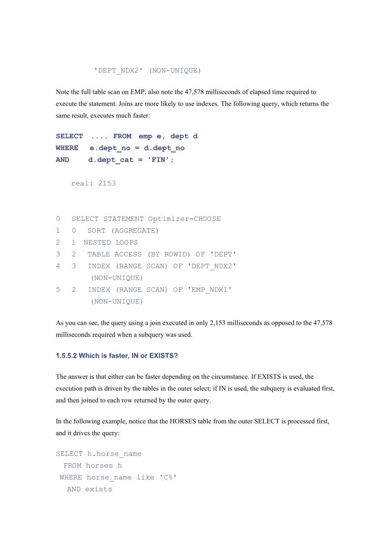
'DEPT_NDX2' (NON-UNIQUE)
Note the full table scan on EMP; also note the 47,578 milliseconds of elapsed time required to
execute the statement. Joins are more likely to use indexes. The following query, which returns the
same result, executes much faster:
SELECT .... FROM emp e, dept d
WHERE e.dept_no = d.dept_no
AND d.dept_cat = 'FIN';
real: 2153
0 SELECT STATEMENT Optimizer=CHOOSE
1 0 SORT (AGGREGATE)
2 1 NESTED LOOPS
3 2 TABLE ACCESS (BY ROWID) OF 'DEPT'
4 3 INDEX (RANGE SCAN) OF 'DEPT_NDX2'
(NON-UNIQUE)
5 2 INDEX (RANGE SCAN) OF 'EMP_NDX1'
(NON-UNIQUE)
As you can see, the query using a join executed in only 2,153 milliseconds as opposed to the 47,578
milliseconds required when a subquery was used.
1.5.5.2 Which is faster, IN or EXISTS?
The answer is that either can be faster depending on the circumstance. If EXISTS is used, the
execution path is driven by the tables in the outer select; if IN is used, the subquery is evaluated first,
and then joined to each row returned by the outer query.
In the following example, notice that the HORSES table from the outer SELECT is processed first,
and it drives the query:
SELECT h.horse_name
FROM horses h
WHERE horse_name like 'C%'
AND exists
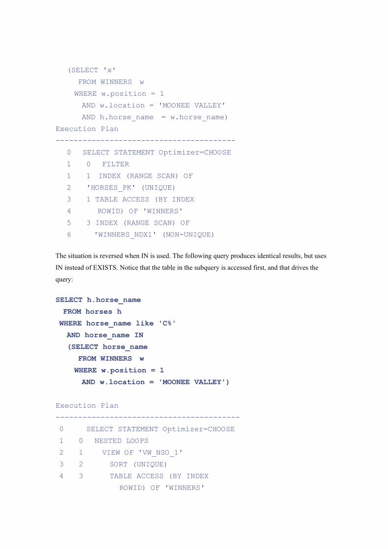
(SELECT 'x'
FROM WINNERS w
WHERE w.position = 1
AND w.location = 'MOONEE VALLEY'
AND h.horse_name = w.horse_name)
Execution Plan
----------------------------------------
0 SELECT STATEMENT Optimizer=CHOOSE
1 0 FILTER
1 1 INDEX (RANGE SCAN) OF
2 'HORSES_PK' (UNIQUE)
3 1 TABLE ACCESS (BY INDEX
4 ROWID) OF 'WINNERS'
5 3 INDEX (RANGE SCAN) OF
6 'WINNERS_NDX1' (NON-UNIQUE)
The situation is reversed when IN is used. The following query produces identical results, but uses
IN instead of EXISTS. Notice that the table in the subquery is accessed first, and that drives the
query:
SELECT h.horse_name
FROM horses h
WHERE horse_name like 'C%'
AND horse_name IN
(SELECT horse_name
FROM WINNERS w
WHERE w.position = 1
AND w.location = 'MOONEE VALLEY')
Execution Plan
-----------------------------------------
0 SELECT STATEMENT Optimizer=CHOOSE
1 0 NESTED LOOPS
2 1 VIEW OF 'VW_NSO_1'
3 2 SORT (UNIQUE)
4 3 TABLE ACCESS (BY INDEX
ROWID) OF 'WINNERS'
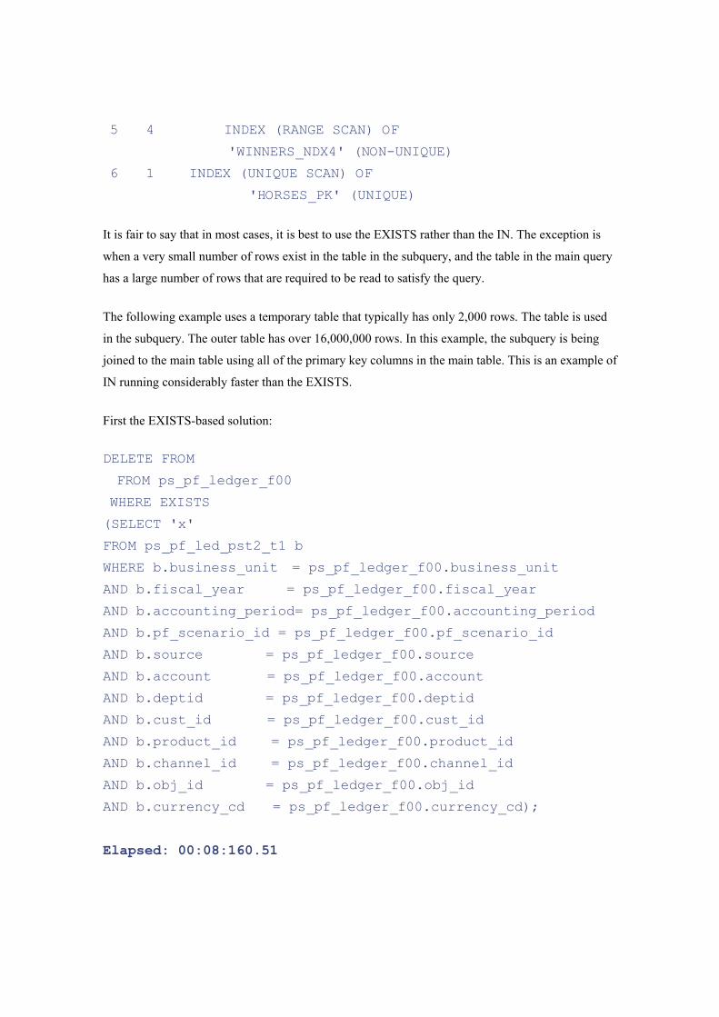
5 4 INDEX (RANGE SCAN) OF
'WINNERS_NDX4' (NON-UNIQUE)
6 1 INDEX (UNIQUE SCAN) OF
'HORSES_PK' (UNIQUE)
It is fair to say that in most cases, it is best to use the EXISTS rather than the IN. The exception is
when a very small number of rows exist in the table in the subquery, and the table in the main query
has a large number of rows that are required to be read to satisfy the query.
The following example uses a temporary table that typically has only 2,000 rows. The table is used
in the subquery. The outer table has over 16,000,000 rows. In this example, the subquery is being
joined to the main table using all of the primary key columns in the main table. This is an example of
IN running considerably faster than the EXISTS.
First the EXISTS-based solution:
DELETE FROM
FROM ps_pf_ledger_f00
WHERE EXISTS
(SELECT 'x'
FROM ps_pf_led_pst2_t1 b
WHERE b.business_unit = ps_pf_ledger_f00.business_unit
AND b.fiscal_year = ps_pf_ledger_f00.fiscal_year
AND b.accounting_period= ps_pf_ledger_f00.accounting_period
AND b.pf_scenario_id = ps_pf_ledger_f00.pf_scenario_id
AND b.source = ps_pf_ledger_f00.source
AND b.account = ps_pf_ledger_f00.account
AND b.deptid = ps_pf_ledger_f00.deptid
AND b.cust_id = ps_pf_ledger_f00.cust_id
AND b.product_id = ps_pf_ledger_f00.product_id
AND b.channel_id = ps_pf_ledger_f00.channel_id
AND b.obj_id = ps_pf_ledger_f00.obj_id
AND b.currency_cd = ps_pf_ledger_f00.currency_cd);
Elapsed: 00:08:160.51
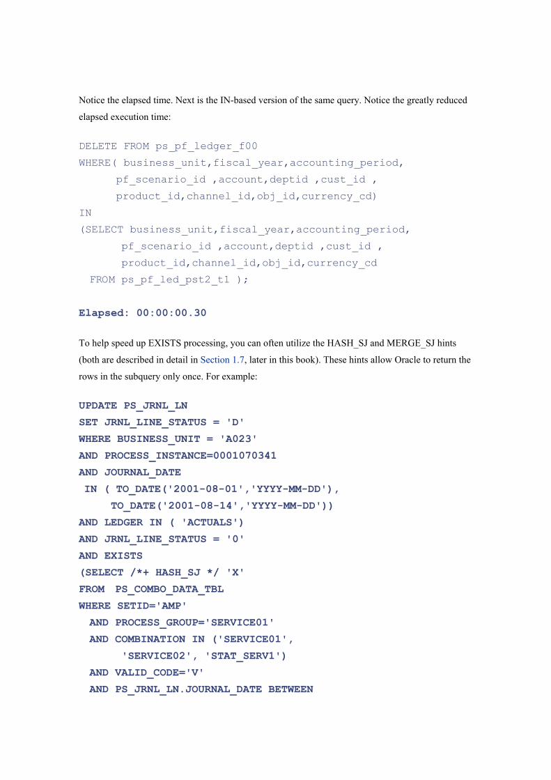
Notice the elapsed time. Next is the IN-based version of the same query. Notice the greatly reduced
elapsed execution time:
DELETE FROM ps_pf_ledger_f00
WHERE( business_unit,fiscal_year,accounting_period,
pf_scenario_id ,account,deptid ,cust_id ,
product_id,channel_id,obj_id,currency_cd)
IN
(SELECT business_unit,fiscal_year,accounting_period,
pf_scenario_id ,account,deptid ,cust_id ,
product_id,channel_id,obj_id,currency_cd
FROM ps_pf_led_pst2_t1 );
Elapsed: 00:00:00.30
To help speed up EXISTS processing, you can often utilize the HASH_SJ and MERGE_SJ hints
(both are described in detail in Section 1.7, later in this book). These hints allow Oracle to return the
rows in the subquery only once. For example:
UPDATE PS_JRNL_LN
SET JRNL_LINE_STATUS = 'D'
WHERE BUSINESS_UNIT = 'A023'
AND PROCESS_INSTANCE=0001070341
AND JOURNAL_DATE
IN ( TO_DATE('2001-08-01','YYYY-MM-DD'),
TO_DATE('2001-08-14','YYYY-MM-DD'))
AND LEDGER IN ( 'ACTUALS')
AND JRNL_LINE_STATUS = '0'
AND EXISTS
(SELECT /*+ HASH_SJ */ 'X'
FROM PS_COMBO_DATA_TBL
WHERE SETID='AMP'
AND PROCESS_GROUP='SERVICE01'
AND COMBINATION IN ('SERVICE01',
'SERVICE02', 'STAT_SERV1')
AND VALID_CODE='V'
AND PS_JRNL_LN.JOURNAL_DATE BETWEEN

EFFDT_FROM AND EFFDT_TO
AND PS_JRNL_LN.ACCOUNT = ACCOUNT
AND PS_JRNL_LN.DEPTID = DEPTID)
UPDATE STATEMENT Optimizer=CHOOSE (Cost=9 Card=1 Bytes=80)
UPDATE OF PS_JRNL_LN
HASH JOIN (SEMI) (Cost=9 Card=1
Bytes=80)
TABLE ACCESS (BY INDEX ROWID) OF
PS_JRNL_LN (Cost=4 Card=1
Bytes=33)
INDEX (RANGE SCAN) OF PSDJRNL_LN
(NON-UNIQUE) (Cost=3 Card=1)
INLIST ITERATOR
TABLE ACCESS (BY INDEX ROWID) OF
PS_COMBO_DATA_TBL (Cost=4
Card=12 Bytes=564)
INDEX (RANGE SCAN) OF
PSACOMBO_DATA_TBL (NON-UNIQUE)
(Cost=3 Card=12)
The Peoplesoft example shown was running for two hours without the HASH_SJ and reduced to an
incredible four minutes with the hint. The hint forces the subquery SELECT rows to be read only
once and then joined to the table outside the subquery (PS_JRNL_LN). The same effect can be
obtained by setting the INIT.ORA parameter ALWAYS_SEMI_JOIN=HASH.
1.5.6 Problem 6: Unnecessary Sorts
Despite a multitude of improvements in the way that Oracle handles sorts, including bypassing the
buffer cache, having tablespaces especially set up as type temporary, and using memory more
effectively, operations that include sorts can be expensive and should be avoided where practical.
The operations that require a sort include the following:
CREATE INDEX
DISTINCT
GROUP BY
ORDER BY
INTERSECT
MINUS
UNIONS
UNINDEXED TABLE JOINS
There are many things a DBA can do to improve sorting, such as making sure that the sorting
tablespace is a TEMPORARY tablespace, having a large SORT_AREA_SIZE to allow more sorts to
occur in memory, ensuring that the default INITIAL and NEXT extents on the TEMP tablespace are
a multiple of the SORT_AREA_SIZE parameter, and ensuring that all users are correctly assigned to
the TEMP tablespace for their sorting.
There are also things that you can do in your SQL to avoid sorts, discussed in the following sections.
1.5.6.1 Consider UNION ALL in place of UNION
Programmers of complex query statements that include a UNION clause should always ask whether
a UNION ALL will suffice. The UNION clause forces all rows returned by the different queries in
the UNION to be sorted and merged in order to filter out duplicates before the first row can be
returned to the calling module. A UNION ALL simply returns all rows, including duplicates, and
does not have to perform any sort, merge, or filtering operations.
Consider the following UNION query:
SELECT acct_num, balance_amt
FROM debit_transactions
WHERE tran_date = '31-DEC-95'
UNION
SELECT acct_num, balance_amt
FROM credit_transactions
WHERE tran_date = '31-DEC-95'
To improve performance, replace this code with the following UNION ALL query:
SELECT acct_num, balance_amt
FROM debit_transactions
WHERE tran_date = '31-DEC-95'
UNION ALL
SELECT acct_num, balance_amt
FROM credit_transactions
WHERE tran_date = '31-DEC-95'
Of course, if your program depends on duplicate rows being eliminated by the database, you have no
choice but to use UNION.
1.5.6.2 Consider using an index to avoid a sort
Indexes can be used to avoid the need to perform sorts. Indexes are stored in ascending order by
default. If the columns in your ORDER BY clause are in the same sequence as the columns in an
index, forcing the statement to use that index will cause the data to be returned in the desired order.
To force the usage of the index, you can either add a hint or use a dummy WHERE clause. Consider
the following statement that executes against a table having an index on (ACC_NAME,
ACC_SURNAME):
SELECT acc_name, acc_surname
FROM account acct
ORDER BY acc_name
The following version of this statement uses a hint to force use of an index:
SELECT /*+ INDEX_ASC(acct acc_ndx1) */ acc_name,
acc_surname
FROM account acct
ORDER BY acc_name
A dummy WHERE clause, on the other hand, is often placed onto online inquiry screens. The
following example uses WHERE acc_name > chr(1) in place of the ORDER BY clause. The
WHERE clause forces the use of the index, which results in rows being returned in sorted order. One
advantage of eliminating the sort in an online application is that the first screenful of rows can be
returned quickly.
SELECT acc_name, acc_surname
FROM account
WHERE acc_name > chr(1)
In a statement like this, there is no need to have the ORDER BY clause. If the ORDER BY clause
was specified, and the user put in a BLANK for his selection and pressed the GO button, every
single row in the table would need to be sorted before a single row could be returned. This could
take a considerable amount of time, and is not desirable behavior in an OLTP environment.
1.5.7 Problem 7: Too Many Indexes on a Table
I've visited sites that have a standard in place saying that no table can have more than six indexes.
This will often cause almost all SQL statements to run beautifully, but a handful of statements to run
badly, and indexes can't be added because there are already six on the table.
Sometimes indexes may be redundant, such as an INDEX_1 on (A, B), INDEX_2 on (A, B, C), and
INDEX_3 on (A, B, C, D). In such cases, DBAs often suggest dropping the first two indexes
because they are redundant; i.e., they have the same leading columns, in the same order, as
INDEX_3. Dropping redundant indexes, however, may cause problems with the selection of a new
driving table on a join using the rule-based optimizer (see the "What the RBO rules don't tell you"
sections earlier in this book). There is far less risk associated with dropping redundant indexes when
the cost-based optimizer is being utilized.
Having lots of indexes on a table will usually have only a small impact on OLTP systems, because
only a few rows are processed in a single transaction, and the impact of updating many indexes is
only milliseconds.
Having lots of indexes can be extremely harmful for batch update processing, with its typically high
number of inserts, updates, and deletes. Table 1-5 demonstrates this.
Table 1-5. Impact of multiple indexes on insert performance
Number of inserts and indexes Runtime
Inserting 256 rows with 0 indexes 1.101 seconds
Inserting 512 rows with 0 indexes 1.161 seconds
Inserting 256 rows with 5 indexes 3.936 seconds
Inserting 512 rows with 5 indexes 12.788 seconds
Inserting 256 rows with 10 indexes 12.558 seconds
Inserting 512 rows with 10 indexes 22.132 seconds
Some sites overcome the problem of having many indexes on a table by dropping all indexes prior to
batch updates, and re-creating them after the batch run is complete. Oracle has added lots of
functionality to help speed index rebuilds. For example, you can rebuild indexes with the
NOLOGGING or UNRECOVERABLE options, and you can rebuild indexes in parallel. Despite
these enhancements, tables may get to a size at which the index rebuild process takes longer than
running a batch update with the indexes intact.
My recommendation is to avoid rules stating that a site will not have any more than a certain number
of indexes.
Oracle9i adds some great new functionality that allows you to identify indexes that are not being
used. The command is ALTER INDEX MONITORING USAGE. Take advantage of it to identify
and remove unused indexes.
The bottom line is that all SQL statements must run acceptably. There is ALWAYS a way of
achieving this. If it requires having 10 indexes on a table, then you should put 10 indexes on the
table.
1.5.8 Problem 8: Use of OR Instead of UNION
When we visit sites to tune SQL, we always seem to identify a few unusual problems that are easily
remedied. The OR EXISTS subquery is just such a headache. We have found statements similar to
the following at several sites:
select .....
from ps_jrnl_header a
where jrnl_hdr_status ='E'
or exists
(select 'x'
from ps_jrnl_header
where business_unit_iu=a.business_unit_iu
and journal_id= a.journal_id
and journal_date=a.journal_date
and unpost_seq= a.unpost_seq
and jrnl_hdr_status='E')
Runtime: 4 Minute 16 seconds
Notice the long runtime for the statement. Wouldn't it be nice to make the statement go faster?
Luckily, the fix is simple. If you have access to change the code (i.e., you are not running a third-
party package), use a UNION statement to implement the OR in the WHERE clause as two separate
queries:
select ...........
from ps_jrnl_header a
where jrnl_hdr_status ='E'
UNION
select .....
from ps_jrnl_header a, ps_jrnl_header b
where b.business_unit_iu
=a.business_unit_iu
and b.journal_id=a.journal_id
and b.journal_date=a.journal_date
and b.unpost_seq=a.unpost_seq
and a.jrnl_hdr_status='E'
and b.jrnl_hdr_status != 'E';
Runtime: 0.02 seconds
The reason for the performance improvement is that the UNION allows the optimizer to perform two
simple operations to return the rows, whereas the more complex OR construct has confused the
optimizer into using a less optimal execution plan.
1.5.9 Problem 9: Tables and Indexes with Many Deletes
Oracle is similar to many other databases in that there are performance issues with deletes. Oracle
has a high water mark, which represents the highest number of rows ever inserted into the table. This
high-water mark can have an impact on performance. Consider the following example, which takes
5.378 seconds to read a table with 151,070 rows:
SELECT COUNT(*) FROM YYYY;
151070
real: 5378
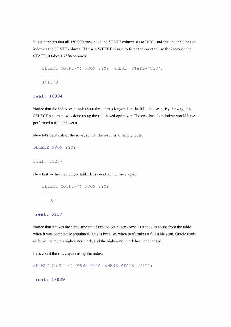
It just happens that all 150,000 rows have the STATE column set to `VIC', and that the table has an
index on the STATE column. If I use a WHERE clause to force the count to use the index on the
STATE, it takes 16.884 seconds:
SELECT COUNT(*) FROM YYYY WHERE STATE='VIC';
---------
151070
real: 16884
Notice that the index scan took about three times longer than the full table scan. By the way, this
SELECT statement was done using the rule-based optimizer. The cost-based optimizer would have
performed a full table scan.
Now let's delete all of the rows, so that the result is an empty table:
DELETE FROM YYYY;
real: 55277
Now that we have an empty table, let's count all the rows again:
SELECT COUNT(*) FROM YYYY;
---------
0
real: 5117
Notice that it takes the same amount of time to count zero rows as it took to count from the table
when it was completely populated. This is because, when performing a full table scan, Oracle reads
as far as the table's high-water mark, and the high-water mark has not changed.
Let's count the rows again using the index:
SELECT COUNT(*) FROM YYYY WHERE STATE='VIC';
0
real: 16029
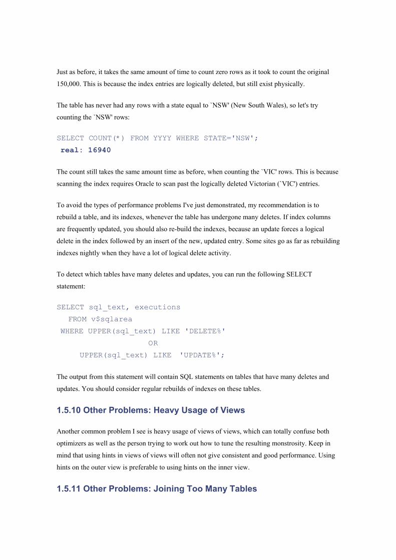
Just as before, it takes the same amount of time to count zero rows as it took to count the original
150,000. This is because the index entries are logically deleted, but still exist physically.
The table has never had any rows with a state equal to `NSW' (New South Wales), so let's try
counting the `NSW' rows:
SELECT COUNT(*) FROM YYYY WHERE STATE='NSW';
real: 16940
The count still takes the same amount time as before, when counting the `VIC' rows. This is because
scanning the index requires Oracle to scan past the logically deleted Victorian (`VIC') entries.
To avoid the types of performance problems I've just demonstrated, my recommendation is to
rebuild a table, and its indexes, whenever the table has undergone many deletes. If index columns
are frequently updated, you should also re-build the indexes, because an update forces a logical
delete in the index followed by an insert of the new, updated entry. Some sites go as far as rebuilding
indexes nightly when they have a lot of logical delete activity.
To detect which tables have many deletes and updates, you can run the following SELECT
statement:
SELECT sql_text, executions
FROM v$sqlarea
WHERE UPPER(sql_text) LIKE 'DELETE%'
OR
UPPER(sql_text) LIKE 'UPDATE%';
The output from this statement will contain SQL statements on tables that have many deletes and
updates. You should consider regular rebuilds of indexes on these tables.
1.5.10 Other Problems: Heavy Usage of Views
Another common problem I see is heavy usage of views of views, which can totally confuse both
optimizers as well as the person trying to work out how to tune the resulting monstrosity. Keep in
mind that using hints in views of views will often not give consistent and good performance. Using
hints on the outer view is preferable to using hints on the inner view.
1.5.11 Other Problems: Joining Too Many Tables
Joining more than five tables will almost always confuse both optimizers, and produce a poor
execution plan. See Section 1.4.5 under Section 1.4. If you are lucky enough to be able to change the
SQL to use hints, you can overcome the problem.
Joining more than five tables frequently in an application usually points to not enough performance
consideration at the design stage, when the logical data model was translated into a physical data
model.
1.6 Handy SQL Tuning Tips
The following sections list some SQL tuning tips that you may find useful both when writing SQL
statements and when troubleshooting performance problems.
1.6.1 Identify Bad SQL
The SQL statements in this section demonstrate how to identify SQL statements that have an
expected response time of more than 10 seconds. The assumption has been made that 300 disk I/Os
can be performed per second, and that 4,000 buffer gets can be performed per second. These times
are typical of a medium- to high-end machine.
Use the following SQL*Plus commands to identify statements using, on average, more than 3,000
disk reads (10 seconds' worth) per execution:
column "Response" format 999,999,999.99;
column nl newline;
ttitle 'SQL With Disk Reads > 10 Seconds'
SELECT sql_text nl, 'Executions='||
executions nl,
'Expected Response Time in Seconds= ',
disk_reads / decode(executions, 0, 1,
executions) / 300
"Response"
FROM v$sql
WHERE disk_reads / decode(executions,0,1, executions)
/ 300 > 10
AND executions > 0
ORDER BY hash_value, child_number;
Similarly, the following SQL*Plus commands identify statements that result in more than 40,000
buffer gets:
column "Response" format 999,999,999.99
ttitle 'SQL Buffer Scan > 10 Seconds'
SELECT sql_text nl, 'Executions='||
executions nl,
'Expected Response Time in Seconds= ',
buffer_gets /
decode(executions, 0, 1, executions)
/ 4000 "Response"
FROM v$sql
WHERE buffer_gets /
decode(executions, 0,1, executions)
/ 4000 > 10
AND executions > 0
ORDER BY hash_value, child_number;
Once you've identified poorly performing SQL statements, you can work to tune them.
1.6.2 Identify Long-Running SQL Statements
Oracle8i and later has a great feature that stores information on long-running queries currently active
in the V$SESSION_LONGOPS view.
The following example shows the results of a query against V$SESSION_LONGOPS:
SELECT username, sql_text, sofar, totalwork, units
FROM v$sql, v$session_longops
WHERE sql_address=address
AND sql_hash_value=hash_value
ORDER BY address, hash_value, child_number
HROA
select count(*) from winners w1, winners_backup w2 where
w1.owner=w2.owner||''
1061 7098 Blocks
In this example, the HROA user is running a SELECT COUNT that is about 15% complete. In other
words, it has processed 1,061 blocks out of 7,098 (1061/7098 = 15%). The statement has been
written to not use an index on the OWNER column of the WINNERS_BACKUP table, because it
has a concatenation against that column. Perhaps the DBA should phone the HROA user and
question the statement, maybe even canceling it if it is going to run for much longer.
1.6.3 Use DECODE for IF/ELSE Selection
Programmers often need a way to count and/or add up variable conditions for a group of rows. The
DECODE statement provides a very efficient way of doing this. Because DECODE is rather
complex, few programmers take the time to learn to use this statement to full advantage. The
following statement uses DECODE to count the number of first, second, and third placings a
racehorse has run:
SELECT horse_name, to_char(sum(decode(position,1,1,0)))
, to_char(sum(decode(position,2,1,0)))
, to_char(sum(decode(position,3,1,0)))
FROM winners
GROUP BY horse_name
In the sum(decode(position,2,1,0)) construct, we are saying that if the horse's finishing position is 2
(second), add one to the count of seconds. The results of this statement appear as follows:
Horse Firsts Seconds Thirds
Wild Charm 1 2 2
The alternative statement without the decode involves scanning the table three times, rather than
once, as in the previous statement.
SELECT horse_name
, count(w1.position)
, count(w2.position)
, count(w3.position)
FROM winners w1, winners w2, winners w3
WHERE w1.horse_name = w2.horse_name
AND w2.horse_name = w3.horse_name
AND w1.position = 1
AND w2.position = 2
AND w3.position = 3
GROUP BY horse_name
1.6.4 Encourage Bind Variables
The values of bind variables do not need to be the same for two statements to be considered identical.
If the bind variable references are the same, the parsed forms of the statements are considered to be
the same. Consequently, the statements share the same parsed form in the shared pool area in
memory.
Following are two sharable SQL statements:
SELECT * FROM emp WHERE emp_no = :B1; Bind value: 123 SELECT * FROM emp WHERE emp_no = :B1; Bind value: 987
These statements are shareable because bind variables have been used, making the statements
themselves identical. The actual bind values do not result in one statement being different from the
other.
Following are two non-sharable SQL statements. These statements are not sharable because bind
variables have not been used, and the resulting hardcoded values make the statements different from
each other.
SELECT * FROM emp WHERE emp_no = 123;
SELECT * FROM emp WHERE emp_no = 987;
In general, encourage your programmers to use bind variables in favor of hardcoding variable values.
This will allow their statements to be stored once in memory rather than once for each distinct
combination of variable values. Coding bind variables may mean extra effort, and should be
attempted only when you are sure that a particular SQL statement will be used repetitively, with the
only difference being bind variable values.
There is one situation in which bind variables are not such a great choice. If you have column data in
a table having a disproportionate number of rows with certain values, and a very small number of
rows with other values, you should be using histograms. Bind variables cannot use histogram
information.
Imagine that you have a three-million row ACCOUNT table that has a SUSPENSE account with one
million rows. All other accounts in the table have an average of a few hundred rows each. It is most
efficient to do a full table scan when a user specifies WHERE ACCOUNT='SUSPENSE' in a
WHERE clause. On the other hand, it is far more efficient to use an index on the ACCOUNT
column if any other account type is selected.
The cost-based optimizer can use histograms to intelligently utilize either the full table scan or the
index scan where appropriate, based on the value specified in the WHERE clause. Using bind
variables will prevent the optimizer from doing this, because the optimizer is unaware of the value
that will be in the bind variable at the time it decides on the execution plan.
Oracle8i introduced a parameter named CURSOR_SHARING. This parameter allows you to
hardcode your WHERE values with literals, numbers, or dates and still have them be shared, and
stored only once in memory. This applies if you have the CURSOR_SHARING parameter set to
FORCE or SIMILAR. Using this parameter, and hardcoding values in your WHERE clauses, will
assist the cost-based optimizer in making substantially better decisions.
Beginning with Oracle9i, the optimizer will consider bind variable values when choosing execution
plans. This avoids having to hardcode values and rely on CURSOR_SHARING = FORCE or
SIMILAR to obtain the advantages of bind variables.
1.7 Using SQL Hints
Hints can be placed into your SQL statements to force the optimizers to utilize a particular execution
path for absolute best performance. The following sections describe available hints up through
Oracle9i.
By including your own optimization hints as "comments" within the SQL statement, you force the
statement to follow your desired retrieval path, rather than the one calculated by the optimizer. In the
following example, including /*+ RULE */ inside the SELECT statement instructs the optimizer to
use the rule-based optimizer rather than the cost-based optimizer:
SELECT /*+ RULE */ . . . .
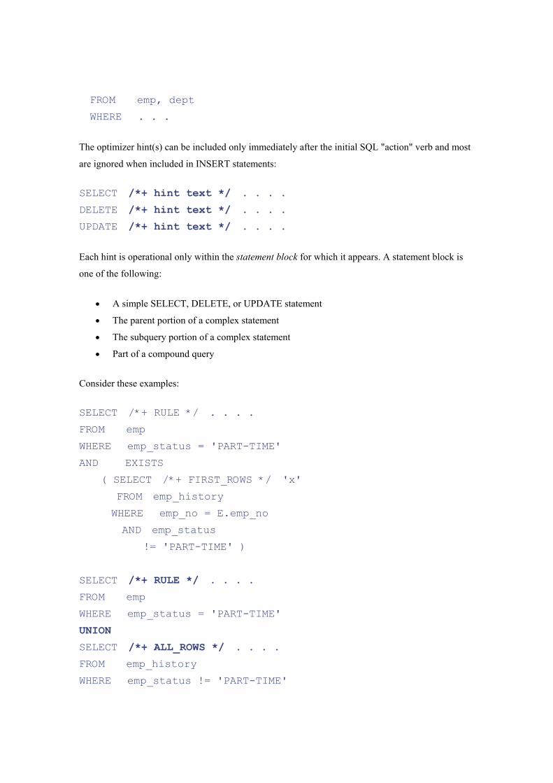
FROM emp, dept
WHERE . . .
The optimizer hint(s) can be included only immediately after the initial SQL "action" verb and most
are ignored when included in INSERT statements:
SELECT /*+ hint text */ . . . .
DELETE /*+ hint text */ . . . .
UPDATE /*+ hint text */ . . . .
Each hint is operational only within the statement block for which it appears. A statement block is
one of the following:
• A simple SELECT, DELETE, or UPDATE statement
• The parent portion of a complex statement
• The subquery portion of a complex statement
• Part of a compound query
Consider these examples:
SELECT /*+ RULE */ . . . .
FROM emp
WHERE emp_status = 'PART-TIME'
AND EXISTS
( SELECT /*+ FIRST_ROWS */ 'x'
FROM emp_history
WHERE emp_no = E.emp_no
AND emp_status
!= 'PART-TIME' )
SELECT /*+ RULE */ . . . .
FROM emp
WHERE emp_status = 'PART-TIME'
UNION
SELECT /*+ ALL_ROWS */ . . . .
FROM emp_history
WHERE emp_status != 'PART-TIME'
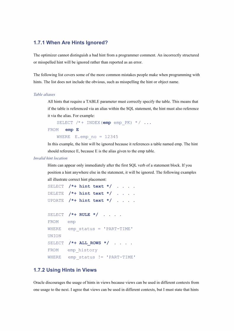
1.7.1 When Are Hints Ignored?
The optimizer cannot distinguish a bad hint from a programmer comment. An incorrectly structured
or misspelled hint will be ignored rather than reported as an error.
The following list covers some of the more common mistakes people make when programming with
hints. The list does not include the obvious, such as misspelling the hint or object name.
Table aliases
All hints that require a TABLE parameter must correctly specify the table. This means that
if the table is referenced via an alias within the SQL statement, the hint must also reference
it via the alias. For example:
SELECT /*+ INDEX(emp emp_PK) */ ...
FROM emp E
WHERE E.emp_no = 12345
In this example, the hint will be ignored because it references a table named emp. The hint
should reference E, because E is the alias given to the emp table.
Invalid hint location
Hints can appear only immediately after the first SQL verb of a statement block. If you
position a hint anywhere else in the statement, it will be ignored. The following examples
all illustrate correct hint placement:
SELECT /*+ hint text */ . . . .
DELETE /*+ hint text */ . . . .
UPDATE /*+ hint text */ . . . .
SELECT /*+ RULE */ . . . .
FROM emp
WHERE emp_status = 'PART-TIME'
UNION
SELECT /*+ ALL_ROWS */ . . . .
FROM emp_history
WHERE emp_status != 'PART-TIME'
1.7.2 Using Hints in Views
Oracle discourages the usage of hints in views because views can be used in different contexts from
one usage to the next. I agree that views can be used in different contexts, but I must state that hints
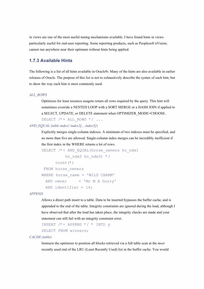
in views are one of the most useful tuning mechanisms available. I have found hints in views
particularly useful for end-user reporting. Some reporting products, such as Peoplesoft nVision,
cannot run anywhere near their optimum without hints being applied.
1.7.3 Available Hints
The following is a list of all hints available in Oracle9i. Many of the hints are also available in earlier
releases of Oracle. The purpose of this list is not to exhaustively describe the syntax of each hint, but
to show the way each hint is most commonly used.
ALL_ROWS
Optimizes for least resource usageto return all rows required by the query. This hint will
sometimes override a NESTED LOOP with a SORT MERGE or a HASH JOIN if applied to
a SELECT, UPDATE, or DELETE statement when OPTIMIZER_MODE=CHOOSE.
SELECT /*+ ALL_ROWS */ ...
AND_EQUAL (table index1 index2[... index5])
Explicitly merges single-column indexes. A minimum of two indexes must be specified, and
no more than five are allowed. Single-column index merges can be incredibly inefficient if
the first index in the WHERE returns a lot of rows.
SELECT /*+ AND_EQUAL(horse_owners ho_ndx1
ho_ndx2 ho_ndx3) */
count(*)
FROM horse_owners
WHERE horse_name = 'WILD CHARM'
AND owner = 'Mr M A Gurry'
AND identifier = 14;
APPEND
Allows a direct path insert to a table. Data to be inserted bypasses the buffer cache, and is
appended to the end of the table. Integrity constraints are ignored during the load, although I
have observed that after the load has taken place, the integrity checks are made and your
statement can still fail with an integrity constraint error.
INSERT /*+ APPEND */ * INTO y
SELECT FROM winners;
CACHE (table)
Instructs the optimizer to position all blocks retrieved via a full table scan at the most
recently used end of the LRU (Least Recently Used) list in the buffer cache. You would
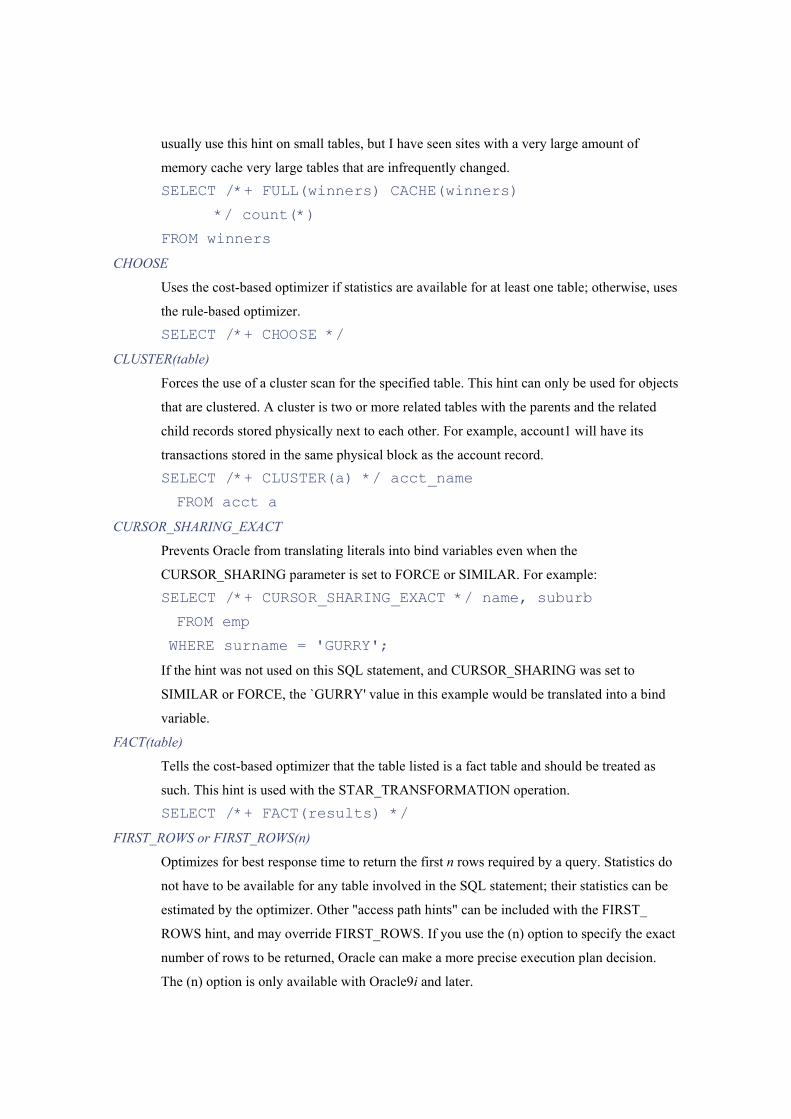
usually use this hint on small tables, but I have seen sites with a very large amount of
memory cache very large tables that are infrequently changed.
SELECT /*+ FULL(winners) CACHE(winners)
*/ count(*)
FROM winners
CHOOSE
Uses the cost-based optimizer if statistics are available for at least one table; otherwise, uses
the rule-based optimizer.
SELECT /*+ CHOOSE */
CLUSTER(table)
Forces the use of a cluster scan for the specified table. This hint can only be used for objects
that are clustered. A cluster is two or more related tables with the parents and the related
child records stored physically next to each other. For example, account1 will have its
transactions stored in the same physical block as the account record.
SELECT /*+ CLUSTER(a) */ acct_name
FROM acct a
CURSOR_SHARING_EXACT
Prevents Oracle from translating literals into bind variables even when the
CURSOR_SHARING parameter is set to FORCE or SIMILAR. For example:
SELECT /*+ CURSOR_SHARING_EXACT */ name, suburb
FROM emp
WHERE surname = 'GURRY';
If the hint was not used on this SQL statement, and CURSOR_SHARING was set to
SIMILAR or FORCE, the `GURRY' value in this example would be translated into a bind
variable.
FACT(table)
Tells the cost-based optimizer that the table listed is a fact table and should be treated as
such. This hint is used with the STAR_TRANSFORMATION operation.
SELECT /*+ FACT(results) */
FIRST_ROWS or FIRST_ROWS(n)
Optimizes for best response time to return the first n rows required by a query. Statistics do
not have to be available for any table involved in the SQL statement; their statistics can be
estimated by the optimizer. Other "access path hints" can be included with the FIRST_
ROWS hint, and may override FIRST_ROWS. If you use the (n) option to specify the exact
number of rows to be returned, Oracle can make a more precise execution plan decision.
The (n) option is only available with Oracle9i and later.
For example:
SELECT /*+ FIRST_ROWS(100) */
This hint:
• Will always choose an index over a full table scan.
• Uses nested loop joins over sort/merge joins, where possible.
• Uses an index to satisfy an ORDER BY clause, where possible.
The optimizer ignores the hints for DELETE and UPDATE statement blocks, and for any
SELECT statement block that contains a "grouping" operation (UNION, INTERSECT,
MINUS, GROUP BY, DISTINCT, MAX, MIN, SUM, etc.) or a FOR UPDATE clause.
Such statements cannot be optimized for best response time, because all rows must be
accessed before the first row can be returned.
FULL(table)
Forces the use of a full table scan on the specified table.
SELECT /*+ FULL(emp) */ ename
FROM emp
WHERE commencement_date > sysdate - 7
If a table has an alias, you must specify the alias name in the hint:
SELECT /*+ FULL(a) */ ename
FROM emp a
WHERE a.commencement_date > sysdate - 7
HASH(table)
Forces the use of a hash table scan for the specified table. This hint applies only to tables
stored in a cluster.
SELECT /*+ HASH(a) */ acct_name
FROM acct a
A lot of people get this hint mixed up with USE_HASH, which forces a hash join. This is
not the same hint!
HASH_AJ
Provides substantial performance improvements by turning a nested loop operation for a
NOT IN into a hash join operation. This hint needs to be placed against the SELECT
statement in the subquery, not in the main select clause.
SELECT count(*)
FROM horses
WHERE horse_name LIKE 'M%'
AND horse_name NOT IN
( SELECT /*+ HASH_AJ */ horse_name
FROM horse_owners
WHERE owner LIKE '%Lombardo%');
HASH_SJ
Often speeds response times in an EXISTS subquery by returning the rows in the subquery
only once.
SELECT count(*)
FROM horses
WHERE horse_name LIKE 'M%'
AND EXISTS
( SELECT /*+ HASH_SJ */ horse_name
FROM horse_owners
WHERE owner LIKE '%Lombardo%'
AND horses.horse_name= horse_owners.horse_name)
There are some restrictions on this hint:
1. There must be only one table listed in the subquery.
2. The hint can't be used in a subquery within a subquery.
3. The subquery must be correlated with an equality predicate, which is a requirement
for all hash joins.
4. The subquery must have no GROUP BY clause, CONNECT BY clause, or
ROWNUM reference.
INDEX(table [index [index...]])
Forces the use of an indexed table scan for the specified table. You can optionally specify
one or more indexes in the hint. If no indexes are included, the optimizer calculates the cost
of all indexes for the table, and uses the most efficient (several indexes may be used in
tandem). If several indexes are listed, the optimizer calculates the cost of only those indexes
that are specified, and uses the most efficient (several indexes from the list may be used in
tandem if they are single-column indexes). If a single index is specified, the optimizer
performs a scan using that index.
SELECT /*+ INDEX(EMP EMP_NDX1) */
SELECT /*+ INDEX(EMP) */
INDEX_ASC(table [index])
Forces the use of an ascending indexed table scan for the specified table. Oracle will scan
indexes in ascending order by default anyway. So why use this hint? Good question! I
suppose this hint guarantees that the index will be traversed in ascending order, even if
Oracle decides to behave differently. The exception to the rule is if the index has been
created as a reverse key index, e.g., CREATE INDEX POST ON OWNERS (ZIPCODE)
REVERSE.
SELECT /*+ INDEX_ASC(EMP EMP_NDX1) */...
INDEX_COMBINE(table [index [index...]])
Explicitly chooses bitmap indexes to access the table information.
SELECT /*+ INDEX_COMBINE(ACCT_TRAN AT_STATE_BMI
AT_TYPE_BMI) */
INDEX_DESC(table [index])
Forces the use of a descending indexed table scan for the specified table. By default, Oracle
scans indexes in ascending sequence. This hint guarantees that the index will be traversed in
descending order. A typical usage of this hint would be to retrieve the latest transactions on
your bank account in descending order by date. This hint can be of great value in distributed
queries.
SELECT /*+ INDEX_DESC(ACCT_TRANS ACCT_TRANS_DATE_NDX)
*/...
INDEX_FFS(table [index])
Instructs the optimizer to do a full scan of an index rather than a full scan of a table. The
index scan can sometimes run faster, but if and only if every column in the WHERE clause
for the specified table exists in the index.
SELECT /*+ INDEX_FFS(ACCT_TRAN AT_STATE_NDX1) */
INDEX_JOIN(table [index] table [index2)]
This hint tells the optimizer to join two indexes as the access path. Typically the execution
plan will include a hash join of the two indexes, which can return some performance
improvements. In the following example, two of the table's three primary key columns have
been used in the WHERE clause (HORSE_NAME and OWNER), as has the leading
column (IDENTIFIER) of a non-primary key index.
SELECT /*+ INDEX_JOIN(HORSE_OWNERS HO_NDX2 HO_PK) */
Horse_name, owner
FROM HORSE_OWNERS
WHERE horse_name = 'WILD CHARM'
AND owner = 'Mr M A Gurry'
AND identifier = 10;
As a matter of interest, without the INDEX_JOIN hint, the optimizers will usually only join
the single-column indexes.
MERGE(table)
Used to force the merging of a nested (inline) view with the main driving query. In the
example given, the GROUP BY inline view is merged with the selection from the
OWNERS table.
The hint can also be used for subqueries if the IN statement is uncorrelated; that is, it does
not reference join columns in the main query.
SELECT /*+ MERGE(w) */ o.owner,
w.num_wins, o.suburb
FROM owners o,
(SELECT owner, count(*) num_wins
FROM winners
WHERE position = 1
GROUP BY owner) w
WHERE o.owner = w.owner
AND w.num_wins > 15
ORDER BY w.num_wins desc
MERGE_AJ
Provides substantial performance improvements by turning a nested loop operation for a
NOT IN into a merge join operation (similar to HASH_AJ). This hint needs to be placed
against the SELECT statement in the subquery, not in the main select clause.
SELECT count(*)
FROM horses
WHERE horse_name LIKE 'M%'
AND horse_name NOT IN
( SELECT /*+ MERGE_AJ */ horse_name
FROM horse_owners
WHERE owner LIKE '%Lombardo%');
MERGE_SJ
This hint will often speed response times in an EXISTS subquery by returning the rows in
the subquery only once.
SELECT count(*)
FROM horses
WHERE horse_name LIKE 'M%'
AND EXISTS
( SELECT /*+ MERGE_SJ */ horse_name
FROM horse_owners
WHERE owner LIKE '%Lombardo%'
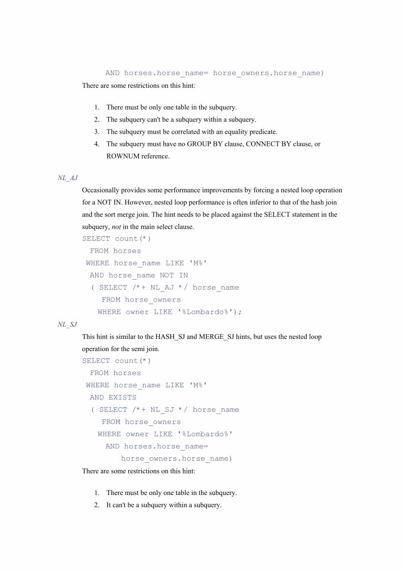
AND horses.horse_name= horse_owners.horse_name)
There are some restrictions on this hint:
1. There must be only one table in the subquery.
2. The subquery can't be a subquery within a subquery.
3. The subquery must be correlated with an equality predicate.
4. The subquery must have no GROUP BY clause, CONNECT BY clause, or
ROWNUM reference.
NL_AJ
Occasionally provides some performance improvements by forcing a nested loop operation
for a NOT IN. However, nested loop performance is often inferior to that of the hash join
and the sort merge join. The hint needs to be placed against the SELECT statement in the
subquery, not in the main select clause.
SELECT count(*)
FROM horses
WHERE horse_name LIKE 'M%'
AND horse_name NOT IN
( SELECT /*+ NL_AJ */ horse_name
FROM horse_owners
WHERE owner LIKE '%Lombardo%');
NL_SJ
This hint is similar to the HASH_SJ and MERGE_SJ hints, but uses the nested loop
operation for the semi join.
SELECT count(*)
FROM horses
WHERE horse_name LIKE 'M%'
AND EXISTS
( SELECT /*+ NL_SJ */ horse_name
FROM horse_owners
WHERE owner LIKE '%Lombardo%'
AND horses.horse_name=
horse_owners.horse_name)
There are some restrictions on this hint:
1. There must be only one table in the subquery.
2. It can't be a subquery within a subquery.
3. The subquery must be correlated with an equality predicate.
4. The subquery must have no GROUP BY, CONNECT BY, or ROWNUM reference.
NO_EXPAND
Prevents a query from being broken up into separate pieces, which is almost the reverse of
the USE_CONCAT hint.
SELECT /*+ NO_EXPAND */ COUNT(*)
FROM horse_owners
WHERE identifier < 10 OR identifier > 20
NO_FACT(table)
Tells the cost-based optimizer that the table listed is not a fact table and should not be
treated as such. This hint is used with STAR_TRANSFORMATION processing.
SELECT /*+ NO_FACT(results) */
NO_MERGE(table)
Prevents the merging of a nested (inline) view.
SELECT /*+ NO_MERGE(w) */ o.owner,
w.num_wins, o.suburb
FROM owners o,
(SELECT owner, count(*) num_wins
FROM winners
WHERE position = 1
GROUP BY owner) w
WHERE o.owner = w.owner
AND w.num_wins > 15
ORDER BY w.num_wins desc
NO_PUSH_PRED(table)
Prevents the join predicate from being pushed into an inline view.
SELECT /*+ NO_PUSH_PRED(v) */ count(*)
FROM horses h,
(SELECT w.horse_name, o.owner,
w.position
FROM winners w, owners o
WHERE w.owner = o.owner) v
WHERE h.horse_name = v.horse_name
AND v.position = 1
NO_UNNEST
Prevents the merging of a subquery into the main statement body. Can only be used when
UNNEST_SUBQUERY=TRUE.
SELECT /*+ NO_UNNEST */ count(*)
FROM horses
WHERE horse_name LIKE 'M%'
AND horse_name NOT IN
( SELECT horse_name
FROM horse_owners
WHERE owner LIKE '%Lombardo%');
NOAPPEND
The opposite of APPEND; results in a conventional insert into a table. There is no guarantee
that the data will be appended at the end of the table. The rows to be inserted do not bypass
the buffer cache, and integrity constraints are respected.
INSERT /*+ NOAPPEND */ * INTO y
SELECT FROM winners;
SELECT /*+ FULL(winners) NOCACHE(winners)
*/ count(*)
FROM winners
NOCACHE(table)
Instructs the optimizer to position all blocks fetched for the specified table at the
leastrecently used end of the LRU list in the buffer cache when performing a full table scan.
This is the normal behavior for a full table scan.
NOINDEX(table [index [index...]])
Eliminates the indexes listed from usage in the execution plan for a query.
SELECT /*+ NOINDEX(EMP EMP_NDX1) */
If a table is specified without an index, no indexes on the table can be used.
SELECT /*+ NOINDEX(EMP) */
NOPARALLEL(table)
Prevents Oracle from using parallelism (multiple processes) to scan the specified table. For
example, assume you enable parallelism as follows:
ALTER TABLE x PARALLEL 2;
Oracle now attempts to use two processes in parallel whenever the table needs to be scanned.
The following statement uses the NOPARALLEL hint to prevent that parallelism from
occurring:
SELECT /*+ NOPARALLEL(x) */ COUNT(*)
FROM x;
NOPARALLEL_INDEX(table, index)
Ensures that parallel index processing does not occur for a partitioned index.
SELECT /*+ NOPARALLEL_INDEX(emp, emp_ndx) */
NOREWRITE
Prevents Oracle from utilizing materialized views based on a selected table. It is the exact
reverse of the REWRITE hint.
SELECT /*+ NOREWRITE */ horse_name, owner, position,
COUNT(*)
FROM results
GROUP BY horse_name, owner, position
ORDERED
Forces the optimizer to join tables in the same order as that in which they are specified in
the FROM clause (left to right). This hint can give enormous performance gains in a
reporting environment. It is also usually the case that the larger the number of tables in the
FROM clause, the larger the benefits from this hint. Following is an example of its use:
SELECT /*+ ORDERED */
acct_name, trans_date, amount,
dept, address
FROM trans t, account a, category c ,
branch b, zip z
WHERE t.trans_date > sysdate - 30
AND a.zip = z.zip
AND z.state = 'WA'
AND t.account between 700000 and
799999
AND t.account = a.account
AND a.account = 'ACTIVE'
AND a.category = c.category
AND c.catgory = 'RETAIL'
AND t.branch_id = b.branch_id
AND b.branch = 'BELLEVUE'
Usually the driving index, and thus the driving table, for a query are determined by the type
of index, how many columns are in the index, the number of rows in the index, and so on.
For example, a table that has a UNIQUE index column equality check in the WHERE
clause will become a driving table over a table that has a NON-UNIQUE column specified
in the WHERE clause.
Interestingly, if all things are equal, the cost-based optimizer will use the left to right order
in the FROM clause, which is the exact reverse of the rule-based optimizer. However, in a
complex query, it is rare to find all things equal in the WHERE clause. Use this hint to
guarantee the join order.
ORDERED_PREDICATES
Causes WHERE clause predicates to be evaluated in the order in which they are listed in the
WHERE clause. If you do not specify ORDERED_PREDICATES, Oracle will evaluate
subqueries and user functions first.
SELECT ...
...
WHERE /*+ ORDERED_PREDICATES */
This is the only hint that goes in the WHERE clause rather than after the keyword that
begins the statement.
PARALLEL(table [,integer] [,integer])
Explicitly specifies the actual number of concurrent query servers that will be used to
service the query. The first optional value specifies the degree of parallelism (number of
query servers) for the table. This is the number of processes assigned to perform the scan of
the specified table in parallel on a single instance. The second optional value specifies the
number of Oracle parallel server instances to split the query across. If you specify
PARALLEL(EMP, 4 2), there will be four parallel query processes running on two separate
parallel server instances. If no parameters are specified, the default (calculated) degree of
parallelism and number of parallel servers is sourced from the parameters specified in the
INIT.ORA file.
The hint can be used for selects, updates, deletes, and inserts. To get performance
improvements using the parallel hint, your datafiles must be striped across multiple disks.
Don't set the degree of parallelism higher than the number of disks that the table is striped
over. Having multiple processors will make the operation run even faster, but only if the
table is striped.
SELECT /*+ PARALLEL (x 4) */ COUNT(*)
FROM x;
SELECT /*+ PARALLEL (x 4 2) */ COUNT(*)
FROM x;
UPDATE /*+ PARALLEL (x 4) */ x
SET position = position+1;
DELETE /*+ parallel(x 4) */ from x;
INSERT INTO x
SELECT /*+ PARALLEL(winners 4) */ *
FROM winners;
PARALLEL_INDEX(table, index, degree of parallelism, cluster split)
Allows you to parallelize index range scans for partitioned indexes. Also allows the work to
be done across multiple instances of a parallel server architecture. The following example
tells the optimizer to utilize parallel index processing on the EMP table, which is partitioned,
to use the EMP_NDX index, and to run at a parallel degree of four over two Oracle parallel
server instances.
SELECT /*+ PARALLEL_INDEX(emp, emp_ndx, 4, 2) */
...
PQ_DISTRIBUTE(table [Outer Distribution] [Inner Distribution])
Used to improve parallel join performance. There are six possibilities for distribution hints,
as listed in Table 1-6.
SELECT /*+ USE_HASH(o)
PQ_DISTRIBUTE(o HASH, HASH) */ COUNT(*)
FROM winners w, owners o
WHERE w.owner = o.owner;
Table 1-6. PQ_DISTRIBUTE combinations
Distribution
combination Meaning
HASH, HASH
Uses a hash function on the join keys for each query server process. Can be used
for a hash join or sort merge join. Works best when tables are approximately the
same size.
BROADCAST,
NONE
Broadcasts all rows of the outer table to each of the parallel query servers. Use
this when the outer table is considerably smaller than the inner table.
NONE,
BROADCAST
Broadcasts all rows of the inner table to each of the parallel query servers. Use
this option when the size of the inner table is much smaller than the outer table.
PARTITION,
NONE
Maps the rows of the outer table using the partitioning of the inner table. The
inner table must be partitioned and equi-joined on the join keys. This option
works most effectively if the number of partitions in the outer table is equal to the
number of parallel query processes utilized.
NONE,
PARTITION
Maps the rows of the inner table using the partitioning of the outer table. The
outer table must be partitioned on the join keys. Use this option when the number
of partitions on the outer table is equal to the number of parallel query servers.
NONE, NONE
Causes each query server to perform a join operation between a pair of matching
partitions, one from each table. Both tables must be equi-partitioned for this
option to be used effectively.
PUSH_PRED(table)
Pushes the join predicate for a table into an inline view. Doing so can sometimes help the
cost-based optimizer make better decisions.
SELECT /*+ PUSH_PRED(v) */ count(*)
FROM horses h,
(SELECT w.horse_name, o.owner,
w.position
FROM winners w, owners o
WHERE w.owner = o.owner) v
WHERE h.horse_name = v.horse_name
AND v.position = 1
The difference in the execution plan for the example is that the HORSE_NAME in the
WHERE clause is joined to the inline view as part of the inline view selection.
PUSH_SUBQ
Forces nonmerged subqueries to be evaluated as early as possible in the execution plan.
Nonmerged subqueries are normally executed as the last step of an execution plan. This hint
has no effect on a subquery if the subquery is over a remote table (as in a distributed SQL
statement), or if the subquery uses a merge join.
SELECT count(*)
FROM horses
WHERE EXISTS
( SELECT /*+ PUSH_SUBQ */ 'x'
FROM horse_owners
WHERE owner LIKE '%Lombardo%'
AND horses.horse_name=
horse_owners.horse_name)
REWRITE
Allows Oracle to utilize materialized views based on a selected table. In the example that
follows, we have a table that contains horse race results. We have created a materialized
view that stores the OWNER, HORSE_NAME, POSITION, and the COUNT(*) for each of
those combinations.
CREATE MATERIALIZE VIEW LOG ON RESULTS
WITH ROWID,
PRIMARY KEY (HORSE_NAME, OWNER,
RACE_DATE)
INCLUDING NEW VALUES;
CREATE MATERIALIZED VIEW winning_horse_owners_vw
USING INDEX
REFRESH ON COMMIT
ENABLE QUERY REWRITE
AS SELECT horse_name, owner, position, COUNT(*)
FROM results
GROUP BY horse_name, owner, position;
In order for this materialized view to be useful, you must have the INIT.ORA parameter
QUERY_REWRITE_ENABLED=TRUE, and the schema MUST HAVE the privilege
QUERY REWRITE assigned. For example:
GRANT QUERY REWRITE TO HROA;
The SQL query shown next is able to obtain all of the data it requires from the view, and
therefore the optimizer will use the view in preference to the table, despite the SELECT
being made against the table.
SELECT /*+ REWRITE */ horse_name, owner, position,
COUNT(*)
FROM results
GROUP BY horse_name, owner, position;
ROWID(table)
Forces a table scan by ROWID for the specified table. The rowid is the physical disk
address of the row.
SELECT /*+ ROWID(a) */ ename
FROM emp a
WHERE rowid > 'AAAGJ2AAIAAABn4AAA'
AND surname like 'GURR%'
RULE
Uses the rule-based optimizer for the current statement block. You can achieve the same
effect by having the CHOOSE option specified for the INIT.ORA parameter
OPTIMIZER_MODE, and not analyzing the tables and indexes used in the SELECT
statement.
STAR
Forces the largest table to be last in the join order. Typically the other tables should be
lookup or reference tables. This hint is used extensively in data warehouse applications.
STAR is only effective when you are joining at least three tables.
SELECT /*+ STAR */ h.horse_name, o.owner,
r.position, r.location, r.race_date
FROM results r, horses h, owners o
WHERE h.horse_name like 'WI%'
AND h.horse_name = r.horse_name
AND r.owner = o.owner;
STAR_TRANSFORMATION
Works on fact and dimension tables, and is similar to the STAR hint. The major difference
is that it allows the cost-based optimizer to decide if it is worth transforming the statement
into a new statement before determining the execution plan. By "transforming," I mean that
the statement is broken into a number of subqueries that are able to take advantage of
bitmap indexes.
To use this hint, it is essential that you have
STAR_TRANSFORMATION_ENABLED=TRUE in your INIT.ORA file.
The most pronounced difference between this hint and the STAR hint is that the
STAR_TRANSFORMATION will often combine bitmap indexes on the various fact table
columns rather than using a Cartesian join. This is achieved by breaking the statement into
subquery pieces.
SELECT /*+ STAR_TRANSFORMATION */
...
UNNEST
Merges the body of a subquery into the body of the main statement, which can often
improve optimizer decision making. UNNEST can only be used when the session parameter
UNNEST_SUBQUERY=TRUE.
SELECT /*+ UNNEST */ count(*)
FROM horses
WHERE horse_name LIKE 'M%'
AND horse_name NOT IN
( SELECT horse_name
FROM horse_owners
WHERE owner LIKE '%Lombardo%');
USE_CONCAT
Forces the optimizer to take OR conditions in the WHERE clause and convert them to a
UNION ALL query operation. In an example such as the one that follows, the index is
scanned twice, once for each condition on the two sides of the OR. The data is then joined
into one result set via a concatenation operation.
SELECT /*+ USE_CONCAT */ COUNT(*)
FROM horse_owners
WHERE identifier < 10 OR identifier > 20
USE_HASH (table)
A hash join is an alternative to a nested loop. A hash table is created in memory of the
smallest table, and then the other table(s) is scanned, with its rows being compared to the
hash. A hash join will run faster than a merge join (sort merge) if memory is adequate to
hold the entire table that is being hashed. The entire join operation must be performed
before a single row is returned to the user. Therefore, hash joins are usually used for
reporting and batch processing.
SELECT /*+ USE_HASH(w o) */ count(*)
FROM winners w, owners o
WHERE w.owner like 'Mr M A Gurry'
AND w.owner= o.owner
AND o.suburb = 'RICHMOND'
A hash join can only be used for equality-based joins (=), and not for range-based joins (<,
<=, >, >=). A merge join is often appropriate when a hash join cannot be used.
Don't confuse the HASH hint with USE_HASH.
USE_MERGE(table)
A merge join is an alternative to nested loop and hash joins. All tables are sorted, unless all
of the columns in the WHERE clause are contained within an index. This sort can be
expensive and it explains why a hash join will often run faster then a merge join.
SELECT /*+ USE_MERGE(w o) */ count(*)
FROM winners w, owners o
WHERE w.owner like 'Mr M A Gurry'
AND w.owner < o.owner
AND o.suburb = 'RICHMOND'
The entire set of data must be returned before a single row is returned to the user. Therefore
hash joins are usually used for reporting and batch processing.
Don't confuse the MERGE hint and USE_MERGE.
Merge joins work effectively for equality-based joins as well as for range-based joins.
Merge joins also often run much faster than a hash join when all of the columns in the
WHERE clause are pre-sorted in an index.
USE_NL(table)
Forces the optimizer to join the specified table to another table (or subquery) using a nested
loop join. The specified table is joined as the inner table of the nested loops. Nested loop
joins are faster than sort/merge or hash joins at retrieving the first row of a query statement.
Online screens should definitely use nested loops, because data will be returned
immediately. As a rule of thumb, if less than 10% of the rows are returned from the tables,
consider using nested loops. Use hash joins or sort merges if 10% or more of the rows are
being returned.
SELECT /*+ USE_NL(w o) */ count(*)
FROM winners w, owners o
WHERE w.owner like 'Mr M A Gurry'
AND w.owner= o.owner
AND o.suburb = 'RICHMOND'
1.8 Using DBMS_STATS to Manage Statistics
DBMS_STATS was introduced in Oracle8i; it provides critical functionality for the cost-based
optimizer, including speeding the analyze process, allowing statistics to be modified, reverting back
to previous statistics, and copying statistics from one schema (or database) to another.
1.8.1 Using DBMS_STATS to Analyze Faster
DBMS_STATS offers two powerful ways of speeding up the analyze process. First, you can analyze
tables (not indexes) in parallel. Second, you can analyze only tables and their associated indexes that
have had more than 10% of their rows modified through INSERT, UPDATE, or DELETE operations.
To analyze a schema's tables in parallel, use a command such as the following:
EXECUTE SYS.DBMS_STATS.GATHER_SCHEMA_STATS (OWNNAME=>
'HROA', ESTIMATE_PERCENT=>10, DEGREE=>4, CASCADE=>TRUE);
This command estimates statistics for the schema HROA. The DEGREE value specifies the degree
of parallelism to use. CASCADE=>TRUE causes the indexes for each table to be analyzed as well.
DBMS_STATS has a GATHER STALE option that will only analyze tables that have had more than
10% of their rows changed. To use it, you first need to turn on monitoring for your selected tables.
For example:
ALTER TABLE WINNERS MONITORING;
You can observe information about the number of table changes for a given table by selecting from
the USER_TAB_MODIFICATIONS view. You can see if monitoring is turned on for a particular
table by selecting the MONITORING column from USER_TABLES.
With monitoring enabled, you can run the GATHER_SCHEMA_STATS package using the
GATHER STALE option:
EXECUTE SYS.DBMS_STATS.GATHER_SCHEMA_STATS (OWNNAME=>
'HROA', ESTIMATE_PERCENT=>10, DEGREE=>4, CASCADE=>TRUE,
OPTIONS=>'GATHER STALE');
Because GATHER_STALE is specified, tables will only be analyzed if they have had 10% or more
of their rows changed since the previous analyze.
1.8.2 Copying Statistics Using DBMS_STATS
DBMS_STATS gives you the ability to copy statistics from one schema to another, or from one
database to another, using the following procedure:
Step 1. Create a table to store the statistics, if you have not already done so:
EXECUTE SYS.DBMS_STATS.CREATE_STATS_TABLE (OWNNAME=>
'HROA', STATTAB=>'HROA_STAT_TABLE');
Step 2. Populate the table with the statistics from the schema that you are copying from:
EXECUTE SYS.DBMS_STATS.EXPORT_SCHEMA_STATS (OWNNAME=>
'HROA', STATTAB=>'HROA_STAT_TABLE', STATID=>
'HROA_21SEP_2001');
Step 3. If you are copying statistics to a different database, such as from production to development,
export and import that statistics table as required:
exp hroa/secret@prod file=stats tables=hroa_stat_table
imp hroa/secret@dev file=stats tables=hroa_stat_table
Step 4. Populate the statistics in the target schema's dictionary. In the following example, statistics
are being loaded for the schema HROA_TEST from the table named HROA_STAT_TABLE:
EXECUTE SYS.DBMS_STATS.IMPORT_SCHEMA_STATS (OWNNAME=>
'HROA_TEST', STATTAB=>'HROA_STAT_TABLE', STATID=>
'HROA_21SEP_2001', STATOWN=> 'HROA');
1.8.3 Manipulating Statistics Using DBMS_STATS
Often you will want to determine if the cost-based optimizer will use the same execution plan in
production as it is using in the current development and test databases. You can achieve this by using
DBMS_STATS.SET_TABLE_STATS to modify the statistics for a table in your development or for
a test database to match those in your production database. The optimizer uses the number of rows,
number of blocks, and number of distinct values for a column to determine whether an index or a
full table scan should be used.
The following example assumes that your production WINNERS table is going to have 1,000,000
rows in 6,000 blocks:
EXECUTE SYS.DBMS_STATS.SET_TABLE_STATS (OWNNAME=>
'HROA_DEV', TABNAME=>'WINNERS', NUMROWS=> 1000000, NUMBLKS=>
6000);
Regardless of how many rows you really have in your test database, the cost-based optimizer will
now behave as if there were 1,000,000.
The optimizer also uses the number of distinct values for each column to decide on index usage. If
the number of distinct values is less than 10% of the number of rows in the table, the optimizer will
usually decide to perform a full table scan in preference to using an index on the table column.
Change the percentage of distinct values for a column as follows:
EXECUTE SYS.DBMS_STATS.SET_COLUMN_STATS (OWNNAME=>
'F70PSOFT', TABNAME=>'PS_LED_AUTH_TBL',
COLNAME=>'OPRID', DISTCNT=>971);
1.8.4 Reverting to Previous Statistics
Usually, re-analyzing a schema and specifying a high percentage of rows for the sample size will
improve performance. Unfortunately, the occasional hiccup will occur when you re-analyze tables.
Sometimes the new statistics produce much worse execution plans than before. You can avoid the
risk of a major screw up by using the DBMS_STATS package to save a copy of your current
statistics just in case you need to restore them later. This requires the following steps:
Step 1. Export your schema statistics to your statistics table. If you don't already have a statistics
table, you can create it using the DBMS_STATS.CREATE_STATS_TABLE procedure. The export
is performed as follows:
EXECUTE SYS.DBMS_STATS.EXPORT_SCHEMA_STATS (OWNNAME=>
'HROA', STATTAB=> 'HROA_STAT_TABLE', STATID=>
'PRE_21SEP_2001');
Step 2. Gather your new statistics:
EXECUTE SYS.DBMS_STATS.GATHER_SCHEMA_STATS (OWNNAME=>
'HROA', ESTIMATE_PERCENT=>10, DEGREE=>4, CASCADE=>TRUE);
Step 3. If there are problems with unsuitable execution paths being selected as a result of the new
statistics, revert back to the previous statistics by loading the previous statistics from the statistics
table:
EXECUTE SYS.DBMS_STATS.IMPORT_SCHEMA_STATS (OWNNAME=>
'HROA', STATTAB=>'HROA_STAT_TABLE', STATID=>
'PRE_21SEP_2001');
1.9 Using Outlines for Consistent Execution Plans
Oracle introduced outlines in Oracle8i to allow you to have a pre-defined execution plan for a SQL
statement. Consistency can then be provided without changing the actual SQL. Outlines can be used
for packaged software to provide execution plan stability without the need to change the
application's SQL.
1.9.1 Recording Outlines
An outline is nothing more than a stored execution plan that Oracle uses rather than computing a
new plan based on current table statistics. Before you can use outlines, you must record some. You
can record outlines for a single statement, for all statements issued by a single session, or for all
statements issued to an instance.
1.9.1.1 Recording an outline for a SQL statement
You can record the outlines for a particular statement using the CREATE OR REPLACE OUTLINE
command as follows:
CREATE OR REPLACE OUTLINE aug0901
FOR CATEGORY harness_racing
ON select *
from winners
where owner > 'G%';
In this example, aug0901 is the name of the specific outline being created, and harness_racing is the
name of a category, or group, or related outlines.
1.9.1.2 Recording outlines for all of a session's SQL
You can turn on the recording of outlines for a session by using the ALTER SESSION
CREATE_STORED_OUTLINES command.
Specify a category name to save outlines into a specific category:
ALTER SESSION
SET CREATE_STORED_OUTLINES
=GENERAL_LEDGER;
Specify TRUE to record outlines in the default category, which is named DEFAULT:
ALTER SESSION
SET CREATE_STORED_OUTLINES=TRUE;
Specify FALSE to disable the recording of stored outlines:
ALTER SESSION
SET CREATE_STORED_OUTLINES=FALSE;
1.9.1.3 Recording outlines for the whole system
The syntax to turn on recording of outlines system-wide is very similar to the ALTER SESSION
syntax. Simply use ALTER SYSTEM instead of ALTER SESSION. For example:
ALTER SYSTEM
SET CREATE_STORED_OUTLINES
=GENERAL_LEDGER NOOVERRIDE;
The NOOVERRIDE option will avoid the complete deletion of the GENERAL_LEDGER outlines
in the example shown. If NOOVERRIDE had not been specified, all statements stored in the
GENERAL_LEDGER category would have been removed. When NOOVERRIDE is specified, new
statements have their outlines added to the existing category. If the same statement appears with an
updated outline, the new outline will be stored.
Likewise, to turn off outline recording system-wide:
ALTER SYSTEM
SET CREATE_STORED_OUTLINES=FALSE;
1.9.2 Enabling Outlines
You now have your outlines stored away. In order for Oracle to use them, you must enable them.
1.9.2.1 Enabling outlines for a session
You can enable the usage of outlines for a session by setting the ALTER SESSION
USE_STORED_OUTLINES command.
Specify a category name to use the outlines in that category:
ALTER SESSION
SET USE_STORED_OUTLINES
=GENERAL_LEDGER;
Specify TRUE to use outlines from the DEFAULT category:
ALTER SESSION
SET USE_STORED_OUTLINES= TRUE;
Specify FALSE to disable (turn off) the use of outlines:
ALTER SESSION
SET USE_STORED_OUTLINES= FALSE;
1.9.2.2 Enabling outlines for the whole system
To enable outlines system-wide, use ALTER SYSTEM instead of ALTER SESSION. Otherwise, the
syntax is the same. For example:
ALTER SYSTEM
SET USE_STORED_OUTLINES
=GENERAL_LEDGER NOOVERRIDE;
In this case, all existing OUTLINES can continue to be used with the GENERAL_LEDGER outlines
that are now used as well. If NOOVERRIDE was not specified, the GENERAL_LEDGER outlines
will replace those currently being used.
Likewise, to disable outlines system-wide:
ALTER SYSTEM
SET USE_STORED_OUTLINES= FALSE;
1.9.3 Managing Outlines
You can view outlines to verify that they have been recording correctly and to see what execution
plan has been recorded. You can also transfer outlines from one schema to another.
1.9.3.1 Viewing your outlines
To view outlines in order to test whether they are recording, select from the OUTLN.OL$ and
OUTLN.OL$HINTS tables. OUTLN.OL$ contains the SQL statements, and OUTLN.OL$HINTS
contains the optimizer hints to use with the statements.
In addition to the tables owned by the OUTLN user, you can also view your own personal outlines
by querying the USER_OUTLINES and USER_OUTLINE_HINTS views (also see the DBA_ and
ALL_ views). For example:
SELECT uo.name, sql_text , hint
FROM user_outlines uo,
user_outline_hints uoh
WHERE uo.name = uoh.name
ORDER BY join_pos
SYS_OUTLINE_010805222913599
select owner ||','|| first ||','|| second ||',' ||third ||','
||points
from winners_current_month
where points > 4
and owner is not null
order by points desc
NO_FACT(WINNERS_CURRENT_MONTH)
To observe if an outline is currently being used for SQL statements, you can look in the
OUTLINE_CATEGORY column of the V$SQL table for the row containing the SQL statement you
are interested in.
1.9.3.2 Transferring outlines between databases
Transferring outlines across databases is simply a case of export and import. For example:
EXP OUTLN/OUTLN FILE=OUTLN_21SEP2001.DMP TABLES=OL$, OL$HINTS
BUFFER=262144
IMP OUTLN/OUTLN FILE=OUTLN_21SEP2001.DMP BUFFER=262144
IGNORE=Y
This example transfers outlines for all schemas. After the import, you can delete rows from the OL$
and OL$HINTS tables in the target database for schemas that you don't wish to transfer.
1.9.3.3 Dealing with literals
Many applications use literals instead of bind variables. This means that SQL statements will often
be similar, and should use the same execution plan. However, since there is one value, the literal
value, different from one statement to the next, that sharing of execution plans does not happen.
Unfortunately, Oracle does not assist us here, even with CURSOR_SHARING = FORCE or
SIMILAR. Cursor sharing does not work for outlines. I am sure that Oracle will address this issue in
the future.