PNNL-17306

T Tank Farm Interim Surface Barrier Demonstration—Vadose Zone Monitoring FY07 Report Z. F. Zhang C. E. Strickland J. M. Keller Pacific Northwest National Laboratory C. D. Wittreich H. A. Sydnor CH2M HILL Hanford Group, Inc. January 2008 Prepared for the U.S. Department of Energy under Contract DE-AC05-76RL01830

DISCLAIMER This report was prepared as an account of work sponsored by an agency of the United States Government. Neither the United States Government nor any agency thereof, nor Battelle Memorial Institute, nor any of their employees, makes any warranty, express or implied, or assumes any legal liability or responsibility for the accuracy, completeness, or usefulness of any information, apparatus, product, or process disclosed, or represents that its use would not infringe privately owned rights. Reference herein to any specific commercial product, process, or service by trade name, trademark, manufacturer, or otherwise does not necessarily constitute or imply its endorsement, recommendation, or favoring by the United States Government or any agency thereof, or Battelle Memorial Institute. The views and opinions of authors expressed herein do not necessarily state or reflect those of the United States Government or any agency thereof.

PACIFIC NORTHWEST NATIONAL LABORATORY operated by

BATTELLE

for the UNITED STATES DEPARTMENT OF ENERGY

under Contract DE-AC05-76RL01830

Printed in the United States of America

Available to DOE and DOE contractors from the Office of Scientific and Technical Information,

P.O. Box 62, Oak Ridge, TN 37831-0062; ph: (865) 576-8401 fax: (865) 576 5728

email: reports@adonis.osti.gov

Available to the public from the National Technical Information Service, U.S. Department of Commerce, 5285 Port Royal Rd., Springfield, VA 22161

ph: (800) 553-6847 fax: (703) 605-6900

email: orders@nits.fedworld.gov online ordering: http://www.ntis.gov/ordering.htm

PNNL-17306

T Tank Farm Interim Surface Barrier Demonstration—Vadose Zone Monitoring FY07 Report Z. F. Zhang C. E. Strickland J. M. Keller Pacific Northwest National Laboratory C. D. Wittreich H. A. Sydnor CH2M HILL Hanford Group, Inc. January 2008 Prepared for the U.S. Department of Energy under Contract DE-AC05-76RL01830 Pacific Northwest National Laboratory Richland, Washington 99352

iii

Executive Summary

CH2M HILL Hanford Group, Inc. is currently in the process of constructing a temporary surface barrier over a portion of the T Tank Farm as part of the T Farm Interim Surface Barrier Demonstration Project. The surface barrier is designed to minimize the infiltration of precipitation into the contaminated soil zone created by the Tank T-106 leak and minimize movement of the contamination. As part of the demonstration effort, vadose zone moisture is being monitored to assess the effectiveness of the barrier at reducing soil moisture. A solar-powered and remotely controlled system was installed to continuously monitor soil water conditions at four locations (i.e., instrument Nests A, B, C, and D) beneath the barrier and outside the barrier footprint as well as site meteorological conditions. Each instrument nest is composed of a capacitance probe with multiple sensors, multiple heat-dissipation units, and a neutron probe access tube. Nests A and B also each contained a drain gauge. The principal variables monitored for this purpose are soil-water content, soil-water pressure, and soil-water flux. Soil temperature, precipitation, and air temperature are also measured. The following table summarizes the monitoring instruments and variables, instrument nests, measurement points, and monitoring frequencies:

Monitoring Instrument Monitoring Variable

Instrument Placement

(Nest) Depth of Sensors/

Measurement Points

Actual Monitoring Frequency

Neutron Moisture Probe Soil-water content A, B, C, D 0.6, 0.9, 1.3, 1.8, and 2.3 m Quarterly

Capacitance Probe Soil-water content A, B, C, D From 1 to 50 ft bgs at 1-ft interval Hourly

Heat Dissipation Unit Soil-Water Pressure A, B, C, D 1, 2, 5, and 9 or 10 m Every 6 hours Heat Dissipation Unit Soil Temperature A, B, C, D 1, 2, 5, and 9 or 10 m Every 6 hours

Drain Gauge Soil-Water Drainage A, B Ground surface Hourly

Thermistor Air Temperature Met Station - Every 15 minutes

Rain Gauge Precipitation Met Station - Every 15 minutes

Each instrument nest is designed to have its own data logger, the data from which are transmitted remotely to the receiving computer. The neutron-probe access tube is used to perform quarterly manual measurements of soil-water content using a neutron probe. Data collected in FY07 reflect baseline conditions without the interim surface barrier in place. All equipment except the drain gauges in Nests A and B was functional while equipment in Nests C and D was installed but had not been hooked up for data collection pending completion of barrier construction. The functionality of Nests C and D has been verified. The monitoring results of Nests A and B in FY07 are summarized below. The capacitance-probe measurements showed that the soil-moisture content at relatively shallow depths (e.g., 0.6 and 0.9 m) was increasing since October 2006 and reached the highest in early January 2007 followed by a slight decrease. Soil-moisture contents at the depths of 1.3 m and deeper were relatively stable during the whole monitoring period. The standard deviations of soil-water content were between 0.003 and 0.015 m3m-3, with smaller variation in deeper soil.

iv

The neutron probe measurements show that the normalized neutron counts had relatively large temporal variation in the soil above 5 ft (1.52 m) bgs but smaller variation in the deeper soil. The heat-dissipation units at the 1.0-m depth showed increasing soil-water pressures in early January before they started decreasing. The peak values of the soil-water-pressure head at the 2-m depth appeared in April 2007 followed by a decrease. The soil-water-pressure heads at 5- and 10-m depths were relatively stable. During FY07, the standard deviations of soil-water-pressure-head were between 0.09 and 1.03 m H2O-height, with generally smaller variations in deeper soil. The heat-dissipation-unit measurements in combination with elevation showed that the soil water was moving downward from late December 2006 to mid-April 2007 and upward at other times in the soil from 1 to 2 m bgs of Nest A. The soil-water movement was always downward below 2 m bgs for Nest A and below 1 m bgs for Nest B. This dominant downward moisture movement indicates that, under the conditions without a surface barrier, the soil was gaining water from precipitation in FY07. Generally, the capacitance probes, neutron probes, and heat-dissipation units showed results that were consistent with the weather conditions. The soil above ~1 m bgs became wetter in the fall of 2006 and winter of 2007 (under wet and cool weather conditions), and drier in the spring and summer of 2007 (under dry and hot weather conditions); the soil from ~1 to ~2 m bgs showed similar seasonal variation but within a smaller range; and the soil-water conditions below ~2 m bgs were relatively stable. The drain gauges did not detect soil-water flux in the T-Farm soil under natural conditions in FY07. However, this does not necessarily indicate zero soil-water flux. Additional tests suggested that either the soil in the gauges has much higher retention properties than expected for a tank farm, or the design of the wick system is not working as expected. Considering that no drain gauges are installed in Nests C and D, which will be under the surface barrier once the barrier is emplaced, the monitoring of the soil-water conditions under the barrier will not be impacted by the lack of measured water fluxes in Nests A and B. It is recommended that 1) neutron probes be calibrated for the access tube used to quantify soil-water content, 2) the 60-cm-depth sensor of the CP in Nest A be moved to a new adjacent location, 3) soil hydraulic properties of the T Farm soil be measured so that the HDU measurements can be used to estimate soil water flux, the 4) water flux meters installed in the T Farm not be considered to estimate the recharge rate, and 5) flux meters to be deployed in the future be tested with field soil in them before commencing monitoring.

v

Acronyms

ARHCO Atlantic-Richfield Hanford Company bgs Below Ground Surface CH2M HILL CH2M HILL Hanford Group, Inc. CP Capacitance Probe FY Fiscal Year HDU Heat-Dissipation Unit HMS Hanford Meteorological Station ID Inside Diameter OD Outside Diameter PMP Project Management Plan PNNL Pacific Northwest National Laboratory QAP Quality Assurance Plan SST Single-Shell Tank STD Standard Deviation

vii

Table of Contents

Executive Summary ..................................................................................................................................... iii

Acronyms...................................................................................................................................................... v

1.0 Introduction....................................................................................................................................... 1.1 1.1 T Farm and T-106 Leak........................................................................................................... 1.1 1.2 Monitoring Nests ..................................................................................................................... 1.2 1.3 Objective and Scope ................................................................................................................ 1.3

2.0 The Vadose Zone Monitoring System .............................................................................................. 2.1 2.1 Monitoring Instruments and Calibration.................................................................................. 2.1

2.1.1 Neutron Probe............................................................................................................. 2.3 2.1.2 Capacitance Probe ...................................................................................................... 2.3 2.1.3 Heat-Dissipation Unit ................................................................................................. 2.4 2.1.4 Water Flux Meter........................................................................................................ 2.5 2.1.5 Precipitation Sensor .................................................................................................... 2.5 2.1.6 Thermistor .................................................................................................................. 2.6

2.2 Monitoring Nests and Installation ........................................................................................... 2.6 2.2.1 Monitoring-Nest Locations and Design...................................................................... 2.6 2.2.2 Instrument Installation ................................................................................................ 2.9

2.3 Monitoring Frequency ........................................................................................................... 2.13 2.4 Data-Analysis Methodology.................................................................................................. 2.13

2.4.1 Removal of Anomalous Data and Error Correction ................................................. 2.13 2.4.2 Temperature-Correction on HDU Measurements..................................................... 2.14 2.4.3 Temperature-Correction on Capacitance-Probe Measurements ............................... 2.14 2.4.4 Normalized Neutron Counts ..................................................................................... 2.15

2.5 Quality Assurance.................................................................................................................. 2.15

3.0 Functionality of the Monitoring System........................................................................................... 3.1 3.1 Battery Voltage........................................................................................................................ 3.1 3.2 Air Temperature ...................................................................................................................... 3.2 3.3 Precipitation............................................................................................................................. 3.2 3.4 Soil Temperature ..................................................................................................................... 3.3 3.5 Soil-Water Flux ....................................................................................................................... 3.5 3.6 Nests C and D .......................................................................................................................... 3.5 3.7 Other Sensors........................................................................................................................... 3.6

4.0 Monitoring Results ........................................................................................................................... 4.1 4.1 Climate Conditions .................................................................................................................. 4.1 4.2 Soil-Water Content .................................................................................................................. 4.2

viii

4.2.1 Capacitance–Probe Measurements ............................................................................. 4.2 4.2.2 Neutron-Probe Measurements .................................................................................... 4.6

4.3 Soil-Water-Pressure Head ..................................................................................................... 4.12 4.4 Soil-Water Flux ..................................................................................................................... 4.15 4.5 Instrument Performance......................................................................................................... 4.15

5.0 Summary and Recommendations ..................................................................................................... 5.1 5.1 System Functionality ............................................................................................................... 5.1 5.2 Soil Water Conditions.............................................................................................................. 5.1 5.3 Recommendations ................................................................................................................... 5.2

6.0 References......................................................................................................................................... 6.1

Figures

1.1. Plan View of T Tank Farm with the Approximate Locations of Monitoring Nests A, B, C, and D, Meteorological Station, and Proposed Interim Surface Barrier Boundary as Marked by the Octagon.................................................................................................................................. 1.2

2.1. Vadose Zone Monitoring Components, Instrumentation, and Data-Collection and Management Flow Diagram for the T Farm Interim Surface Barrier Demonstration Project................................ 2.2

2.2. Typical Instrument Surface Completion Showing Outer 24-In.-Diameter Corrugated Metal Pipe Sleeving and Inner Steel Casing ....................................................................................................... 2.7

2.3. Cone-Tipped Drive Shaft Used in Conjunction with a Hydraulic Hammer for Creating Driving Boreholes .......................................................................................................................................... 2.9

2.4. Hydraulic Hammer Used to Install Instruments in the T Tank Farm ............................................... 2.9

2.5. Diagram of the Installed Neutron Probe Access Tubes (i.e., 2.5-in. steel casing) for Nest C and Nest D) ..................................................................................................................................... 2.10

2.6. Diagram of the Installed Capacitance Probe Access Tubes Surrounded by 20/40 Sand Backfill for Nest C and Nest D..................................................................................................................... 2.11

2.7. HDU Installation and Packing Material Layering Scheme for Nests C and D............................... 2.12

3.1. Daily Average Battery Voltage......................................................................................................... 3.1

3.2. Daily Average Air Temperature ....................................................................................................... 3.2

3.3. Cumulative Precipitation Starting December 14, 2006, at the T Tank Farm and Hanford Meteorological Station...................................................................................................................... 3.3

ix

3.4. Daily Average Soil Temperature at Different Depths Measured Using the HDUs .......................... 3.4

4.1. Monthly Precipitation (mm) in Hanford ........................................................................................... 4.1

4.2. Monthly Air Temperature (°C) in Hanford....................................................................................... 4.2

4.3. Daily Average Soil-Water Content at Five Depths Measured Using the CPs .................................. 4.3

4.4. Soil-Water Content Profiles for Nests A and B on Selected Dates for CPs ..................................... 4.4

4.5. Normalized Neutron Counts Measured Using Neutron Probes at Different Depths of Nest A........ 4.7

4.6. Normalized Neutron Counts Measured Using Neutron Probes at Different Depths of Nest B ........ 4.8

4.7. Normalized Neutron Counts Measured Using Neutron Probes at Different Depths of Nest C ........ 4.9

4.8. Normalized Neutron Counts Measured Using Neutron Probes at Different Depths of Nest D...... 4.10

4.9. Comparison of Normalized Neutron Counts Measured Using Neutron Probes on July 11, 2007................................................................................................................................... 4.11

4.10. Daily Average Soil-Water Pressure at Different Depths Measured Using the HDUs.................... 4.12

4.11. Soil-Water-Pressure Head Profiles for Nests A and B on Selected Dates Using the HDUs .......... 4.13

4.12. Daily Average Soil-Water Hydraulic Head at Different Depth Intervals Determined Using the Measurements of the HDUs...................................................................................................... 4.14

Tables

2.1. Instruments Selected for Interim Surface Barrier Monitoring and the Monitored Variables ........... 2.2

2.2. Capacitance Sensor Frequency Readings in Air and Water ............................................................. 2.4

2.3. Vadose Zone Monitoring Borehole Coordinates and Associated Installed Instruments .................. 2.8

2.4. Instrument Vertical Placement.......................................................................................................... 2.8

2.5. Serial Numbers of the Capacitance Sensors Installed in Nests A, B, C, and D................................ 2.8

2.6. Serial Numbers and Sensor Numbers of the HDU Sensors Installed in Nests A, B, C, and D......... 2.9

2.7. Data-Collection Method(a) and Approximate Frequency Under Normal Working Conditions ...... 2.13

3.1. The HDU-Measured Average (Tavg), Minimum (Tmin), Maximum (Tmax), and Standard Deviation (STD) of Soil Temperature for Nests A and B................................................................. 3.5

x

4.1. The Average (θavg), Minimum (θmin) and Maximum (θmax) and Standard Deviation (STD) of Soil-Water Content for Nests A and B ............................................................................................. 4.5

4.2. The Depth-Averaged Normalized Neutron Counts for Nest A......................................................... 4.5

4.3. The depth-Averaged Normalized Neutron Counts for Nest B.......................................................... 4.5

4.4. The Depth-Averaged Normalized Neutron Counts for Nest C......................................................... 4.6

4.5. The Depth-Averaged Normalized Neutron Counts for Nest D......................................................... 4.6

4.6. The HDU-Measured Average (ψavg), Minimum (ψmin), Maximum (ψmax), and Standard Deviation (STD) of Soil-Water-Pressure Head for Nests A and B................................................. 4.13

4.7. Instrument Performance.................................................................................................................. 4.15

1.1

1.0 Introduction

The Hanford Site in southeastern Washington State has 149 underground single-shell tanks (SSTs) that store hazardous radioactive waste. Many of these tanks and their associated infrastructure (e.g., pipelines, diversion boxes) have leaked. The largest known leak occurred from Tank T-106 in 1973. Many of the contaminants from that leak still reside within the vadose zone beneath the T Tank Farm. CH2M HILL Hanford Group, Inc. (CH2M HILL) seeks to minimize movement of this residual contaminant plume by placing an interim barrier on the ground surface to minimize the infiltration of precipitation. The temporary surface barrier is being constructed as part of the T Farm Interim Surface Barrier Demonstration Project. Vadose zone moisture is being monitored to assess the effectiveness of the surface barrier at reducing soil moisture beneath the barrier. The technology being used to create the impermeable barrier is a spray-polyurea liner material. Construction of the surface barrier is expected to be completed in the spring of 2008. This report presents soil-moisture data that have been collected from October 2006 to September of 2007 (FY07) that are representative of baseline conditions before placing the barrier. Such baseline data will provide for future comparison of data after the interim surface barrier is emplaced. Also presented is a description of two new instrument nests installed in September 2007 to support the monitoring initiative.

1.1 T Farm and T-106 Leak According to Myers (2005), the T tank farm was built from 1943 to 1944. The T tank farm contains 12 SSTs with a diameter of 23 m (75 ft) and a capacity of 2,006,050 L (530,000 gal), four SSTs with a diameter of 6.1 m (20 ft) and a capacity of 208,175 L (55,000 gal), waste-transfer lines, leak-detection systems, and tank ancillary equipment. The soil cover from the apex of the tank domes to the ground surface is approximately 2.2 m (7.3 ft). All the tanks have a dish-shaped bottom. In general, the vadose zone in the T tank farm consists of a portion of the thick, relatively coarse-grained sediments of the middle Ringold Formation (Rwi) overlain by the finer grained sediments of the upper Ringold Formation (Rtf) and the Plio-Pleistocene unit (also called the Cold Creek Unit). This in turn is overlain by the coarser grained sands and gravels of the Hanford formation, which are exposed at the surface. The upper 12 m (40 ft) of the Hanford formation was locally excavated and redeposited as backfill material around the tanks. A leak from Tank T-106 occurred in 1973, and the details and chronology of the leak are well documented (ARHCO 1973; Routson et al. 1979). The leak was suspected to have started on April 20, 1973, during a routine filling operation. The leak stopped on June 10, 1973, when the free liquid contents of the tank were removed. The total duration of the leak was estimated to be 51 days. Approximately 435,000 L (115,000 gal) of fluid leaked from Tank T-106. The fluid contained cesium-137, strontium-90, plutonium, and various fission products, including technetium-99. It is likely that the leak occurred in the southeast quadrant of the tank near the bottom of the tank side (Routson et al. 1979). It is expected that the interim surface barrier will minimize the meteoric water entering into soil and consequently will reduce the rate of downward movement of antecedent water and transport of contaminants (McMahon 2007). At shallower depths, there will be no water supply from above to replace the draining antecedent pore water, and hence, at the shallow zone, the soil will dry more quickly. In

1.2

deeper soil zones, the soil will continue to receive drainage from the soil above for some time and will drain more slowly. Therefore, it may take years for drainage rates deep in the profile (e.g., > 10 m bgs) to reduce significantly. As the soil below the surface barrier becomes drier, the soil directly beneath the barrier edge will also become drier than would be the case were there no surface barrier.

1.2 Monitoring Nests During August and September of 2006, Nests A and B (Figure 1.1) of the vadose zone monitoring system were installed within the T Tank Farm, and a meteorological station was installed outside of the tank farm. In September of 2007, Nests C and D (Figure 1.1) of the vadose zone monitoring system were installed, but have not been hooked up to dataloggers and/or batteries. Each of the four instrument nests are designed to include its own datalogger as is the meteorological station outside the farm.

T-106

Approximate Barrier Footprint

Lined Runoff Ditch

RunoffInfiltration Area

Instrumentation Nests A

B

C D

Meteorological Station

Figure 1.1. Plan View of T Tank Farm with the Approximate Locations of Monitoring Nests A, B, C,

and D, Meteorological Station, and Proposed Interim Surface Barrier Boundary as Marked by the Octagon

1.3

1.3 Objective and Scope The objective of the report is to present the baseline data collected from Nests A and B of the four subsurface instrument nests (Figure 1.1) through FY07 in accordance with the T Tank Farm Interim Surface Barrier Demonstration – Vadose Zone Monitoring Plan (Zhang et al. 2007), which will be referred to as the Monitoring Plan hereafter. The baseline data will be used to compare against data collected from instrument Nests C and D after the interim surface barrier is installed. Additionally, this report provides installation and location details for two instrument nests (Nests C and D) installed in September 2007. Nests A and B were installed in FY06 as described in the Monitoring Plan. Data from all nests will ultimately be used to evaluate the impacts of the interim surface barrier on sub-surface moisture conditions. Chapter 2 of this report summarizes the monitoring instruments, pertinent calibration information, instrument installation methods, and data-analysis methodology. Chapter 3 summarizes the functionality of the monitoring system. Chapter 4 presents the monitoring baseline results of the primary variables, i.e., the soil-water content measured by the capacitance probe (CP), the normalized neutral counts by the neutron probe, the soil-water-pressure head by the heat dissipation unit (HDU), and soil-water flux by the drain gauge. Chapter 5 summarizes instrument functionality and results of measured soil-water conditions and presents recommendations for future monitoring activities.

2.1

2.0 The Vadose Zone Monitoring System

Soil-moisture conditions were monitored using an array of solar-powered and remotely controlled instrument nests and neutron-probe access tubes located beneath and outside of the interim barrier. The principal variables monitored for this purpose are soil-water content (θ), soil-water pressure (ψ), and soil-water flux (q). The reasons for selecting these variables were given in Section 3.1 of the Monitoring Plan. Briefly, each variable reflects one aspect of the soil-moisture regime; their variation is different under different conditions; and soil-water flux is directly related to the transport velocity of the dissolved solute. The measurement of three different variables also serves as a redundancy of monitoring. Secondary variables monitored include soil temperature and meteorological conditions, including precipitation and air temperature. The measured precipitation will be used to estimate the total volume of water intercepted by the surface barrier after construction is complete. Soil temperature is used to correct the temperature impact on θ and ψ, and along with air temperature, to assess system functionality. To fulfill the purpose of monitoring surface-barrier impacts on the subsurface water regime, multiple instrument nests were installed both under the interim surface barrier and outside of the surface barrier, as described in Section 5.1 of the Monitoring Plan. Spatial variability of soil properties and measurement error were considered and were minimized by one of more of the following: 1) using measurements of different types (i.e., θ, ψ, and q), 2) taking multiple measurements in the vertical direction (e.g., θ and ψ), 3) duplicating instrument nests (e.g., Nests C and D), 4) measuring the same variable with more than one method (e.g., θ is measured using CPs and neutron probes), and 5) measuring the variation with time at desired frequency (for all the variables). The Monitoring Plan presented the criteria used to select the various measurement methods, the principles of selected methods (Section 3.0), part of the instrument calibrations (Section 4.0), instrument layout and installation of Nests A and B (Section 5.0), and measurement procedures and frequencies (Section 6.1). In FY07, more sensors were calibrated, and two more instrument nests (C and D) were installed. For convenience for the readers and completeness, this section summarizes the monitoring instruments, pertinent calibration information, instrument installation methods, and data-analysis methodology.

2.1 Monitoring Instruments and Calibration Monitoring instruments were chosen based on several considerations. Primary considerations used to select instrumentation are that the instrumentation is amenable to the prescribed installation method (hydraulic hammer) and restrictions of working within the T tank farm. Additional criteria considered are described in Table 3.1 of the Monitoring Plan. Table 2.1 lists the instruments selected for use and the variables monitored by each instrument. Figure 2.1 shows monitoring components, instrumentation, and a data-collection and management flow diagram. In the following sections, each instrument is briefly described, and supporting calibration information is provided.

2.2

Table 2.1. Instruments Selected for Interim Surface Barrier Monitoring and the Monitored Variables

Instrument Manufacturer Model Variable Monitored

Measurement Precision

Neutron Probe Campbell Pacific Nuclear

503DR Hydroprobe

Soil Moisture Content ±0.016 m3m-3

Capacitance Probe Sentek EnviroSMART Soil Moisture Content ±0.01 m3m-3

Heat Dissipation Unit

Campbell Scientific, Inc. 229-L Soil-Water Pressure,

Soil Temperature ±20%

±0.25°C

Water Fluxmeter Decagon Devices, Inc Drain Gauge Soil Water Flux ±10% (1 ml

resolution) Precipitation

Sensor Texas Electronics TE525WS Precipitation ±1%

Thermistor Campbell Scientific, Inc. 109-L Air Temperature ±0.1°C

Meteorological ConditionsSoil Water Pressure Soil Water Content

Soil Water DrainageSoil Temperature

Air Temperature Precipitation

HDU Capacitance Probe

Neutron Probe HDU Drain Gauge Thermister Rain Gauge

Datalogger RF Telemetry and Telephone

Central Database

Post Processing

Analysis

Reporting

Monitoring Components

Instruments

Data Collection and Management

Figure 2.1. Vadose Zone Monitoring Components, Instrumentation, and Data-Collection and

Management Flow Diagram for the T Farm Interim Surface Barrier Demonstration Project

2.3

2.1.1 Neutron Probe Neutron thermalization, as a method to measure soil-water content, uses a radioactive source of fast neutrons (mean energy of 5 MeV) and a detector of slow neutrons (~0.025 eV). High-energy neutrons emitted from the source are either slowed through repeated collisions with the nuclei of atoms in the soil (scattering) or are absorbed by those nuclei. The most common elements in soil (Al, Si, and O) scatter neutrons with little energy loss. If the neutron hits a hydrogen (H) atom, its energy is reduced on average by about half because the mass of the H nucleus is the same as that of the neutron. The concentration of thermal neutrons changes mainly with the H content of the surrounding material, while changes in H content occur mainly because of changes in soil-water content. Therefore, the concentration of thermal neutrons surrounding a neutron source placed in the soil can be related to the soil volumetric water content. Neutron-probe monitoring of the T-Farm interim surface barrier uses a 503DR hydroprobe manufactured by CPN International, Inc. (Martinez, CA), which was described in detail in Section 3.3.1 of the Monitoring Plan. The 2.5-inch-OD, 0.375-inch-thick steel casings are used for neutron probe access.

2.1.2 Capacitance Probe The CP is an electromagnetic method used to measure the volumetric soil-water content (θv) of the surrounding soil. The capacitance method uses the soil surrounding the electrodes as part of a capacitor in which the dipoles of water in the soil become polarized in response to the frequency of an imposed electric field. Hence, oscillation frequency is a function of soil-water content. The CP used for the T-Farm interim surface barrier monitoring is the EnviroSMART probe (Sentek Pty Ltd, Stepney, Australia), which was described in detail in Section 3.3.2 of the Monitoring Plan. Two components exist as part of the EnviroSMART CP calibration: 1) a normalization process to minimize instrumental-dependent readings and 2) a calibration process to relate the soil-water content with the normalized frequency. For cylindrical sensors, a normalized frequency (Sf) is calculated by incorporating the raw-frequency reading in soil (F) with frequency readings in air (Fa) and in water (Fw) (Paltineanu and Starr 1997):

wa

af FF

FFS−−

= (2.1)

Table 2.2 presents the water and open-air measurement output for each sensor. The measurements for the 15 sensors listed in the left half of Table 2.2 were the same as those in Table 4.1 of the Monitoring Plan, while the 10 sensors in the right half were new values obtained in FY07. The CP calibration documentation (Sentek Pty Ltd. 2001) provides a default calibration developed using sand, loam, and clay-loam soils. This calibration was developed by performing nonlinear regression on frequency data for paired volumetric moisture content and normalized frequency:

bf

v acS /1

⎟⎟⎠

⎞⎜⎜⎝

⎛ −=θ (2.2)

2.4

where a = 0.1957, b = 0.4040, and c = 0.02852. The general calibration can also be used in gravelly soils (e.g., the T Farm soils) because capacitance probes are relatively insensitive to gravel content (Baumhardt et al. 2000).

Table 2.2. Capacitance Sensor Frequency Readings in Air and Water. Values are used to normalize capacitance sensor output using Eq. (2.1).

Frequency Frequency Sensor Serial # Air Water Sensor Serial # Air Water

AP06-303 37584 28503 FE06-451 35956 27169 AP06-304 37170 28219 FE06-452 36556 27383 AP06-305 37522 28657 FE06-453 36275 27152 AP06-309 37728 28863 FE06-454 36451 27641 AP06-310 37583 28413 FE06-455 36713 27817 FE06-371 37448 28395 FE06-456 37535 27134 FE06-372 37048 28148 FE06-457 36751 27148 FE06-373 37323 28227 FE06-458 36225 27622 FE06-374 37720 28468 FE06-459 38346 28328 FE06-375 37180 27835 FE06-460 37643 27621 FE06-376 37162 28246 FE06-377 37468 28374 FE06-378 37545 28517 FE06-379 37359 28270 FE06-380 37381 28456

2.1.3 Heat-Dissipation Unit An HDU indirectly measures the soil matric potential (ψs) by measuring the thermal conductivity of the reference matrix, which is part of an HDU and is made of porous ceramics. HDU measurement and calibration are independent of soil texture because the heat pulse is restricted to the ceramic. It is also independent of salinity because the method is independent of electrical conductivity. HDUs have the added benefit of also measuring soil temperature. HDUs consist of a heater and a temperature sensor in a porous ceramic. The temperature rise measured by the temperature sensor at time t represents the heat that is not dissipated at this time. The time dependence of temperature, T, in a line heat source buried in an infinite medium can be approximated by the method of Shiozawa and Campbell (1990):

)ln(4 00 tt

kqTTT −=−=Δπ

(2.3)

where T and T0 are the temperatures at time t and t0, respectively, q is the heat input, and ΔT is temperature rise. The HDU used for the T-Farm interim surface barrier monitoring is the model 229-L

2.5

HDU manufactured by Campbell Scientific, Inc. (Logan, UT), which was described in detail in Section 3.4 in the Monitoring Plan. Similar to the CP, there are two elements to the HDU calibration: 1) a normalization procedure to remove variation between the HDU sensors and 2) a calibration procedure to develop the relationship between soil-water pressure head and the normalized temperature rise measured by the HDU. The normalization procedure of Flint et al. (2002) was used to calculate the normalized temperature rise (SΔT), according to:

wd

dT TT

TTSΔ−ΔΔ−Δ

=Δ (2.4)

where subscripts “d” and “w” denote the temperature rises for a dry and water-saturated ceramic matrix, respectively. The HDU temperature-rise measurement under dry conditions (ΔTd) was made after the HDU had been placed over oven-dried desiccant in a sealed container for a length of time (approximately 24 hours). For the HDU temperature-rise measurement under water-saturated conditions (ΔTw), the sensor was submerged in water for 24 to 48 hours and then removed before the HDU measurement. All readings were taken with a constant line-heat source current of 50 mA and measurement times of 1 s and 30 s after HDU heating was initiated. Details of sensor normalization and calibration are given in Section 4.3 of the Monitoring Plan. Using the normalized HDU temperature rise, SΔT, and tensiometer-measured matric potential, ψ (m of water), under steady-state soil conditions, a calibration was developed (Eq. 4.2 in the Monitoring Plan):

2548.69697.3388.12 2 −×−×= ΔΔ TT SSψ , r2 = 0.9689 (2.5)

2.1.4 Water Flux Meter A water-flux meter measures the downward soil-water flux or drainage of water within the soil profile. The convective movement of water controls the downward movement of contaminants at Hanford, and thus, soil-water flux is a measure of mobile contaminant-transport potential. The flux meter used for the T-Farm interim surface barrier monitoring is the drain gauge manufactured by Decagon Devices, Inc. (Pullman, WA), which is described in detail in Section 3.5 of the Monitoring Plan.

2.1.5 Precipitation Sensor Monitoring precipitation directly at the T Tank Farm is useful in determining the total amount of meteoric water and the amount of water intercepted by the surface barrier. Localized thunderstorms that occasionally occur at Hanford produce spatially variable short-term, high-energy precipitation events. The possibility of such events requires that a meteorological monitoring station be located at the T Farm to document potential localized precipitation events. The rain gauge installed at the T Tank Farm for this purpose is a tipping-spoon type rain gauge, model TE525WS, manufactured by Texas Electronics (Dallas, TX). Power requirements needed for a heated rain gauge necessitated that the rain gauge not be heated because there is no available AC power. As such, the rain gauge may not accurately measure precipitation during periods of snowfall. Given the proximity of the Hanford Meteorological Station (HMS) and the uniformity of snowfall across the Hanford Site, it is acceptable to conclude that snowfall measured by the HMS will approximately describe the snowfall at

2.6

the T farm. The rain-gauge tipping spoon is factory calibrated to an equivalent depth of water of 0.254 mm per tip.

2.1.6 Thermistor A thermistor is a resistor that relies on the change in its resistance with changing temperature to measure temperature. Two different Campbell Scientific, Inc. models of thermistors are used for interim surface barrier monitoring, the Model 107 and the Model 109. The Model 107 temperature probe is used as a reference temperature probe and is located within the enclosure boxes housing the dataloggers that control the instruments inside the T Tank Farm. The Model 107 temperature probe is described by a fifth-order polynomial equation relating thermistor resistance, Rs (Ohms), to temperature, T (°C) by (Campbell Scientific Inc. 2004),

55

44

33

2210 sssss RCRCRCRCRCCT +++++= (2.6)

where C0 = -53.4601, C1 = 90.807, C2 = -83.257, C3 = 52.283, C4 = -16.723, and C5 = 2.211. The Model 109 temperature probe is used as part of the meteorological station. This temperature sensor relates thermistor resistance to temperature (°C) using the relationship (Campbell Scientific Inc. 2004),

( )[ ]15.273

ln)ln(1

3 −⎭⎬⎫

⎩⎨⎧

++=

RsCRsBAT (2.7)

where A = 1.129241×10-3, B = 2.341077×10-4, and C = 8.775468×10-8.

2.2 Monitoring Nests and Installation This section describes the location and composition of the instrument nests and summarizes the installation procedure.

2.2.1 Monitoring-Nest Locations and Design Figure 1.1 provides a plan view of instrument-nest locations and the planned footprint of the interim surface barrier. In accordance with the Monitoring Plan, four subsurface monitoring instrument nests were located both under and outside of the surface barrier (i.e., A, B, C, and D; denoted as 1, 2, 3, and 4, respectively, in CH2M HILL 2006, 2007). Each nest includes a neutron access tube, a CP with five sensors, and four HDUs. Nest A is placed in the area outside the barrier footprint and serves as a control, providing subsurface conditions outside the influence of the surface-barrier. It is approximately 10 m away from the closest edge of the surface barrier, which is a sufficient distance to prevent measurable impacts from the surface barrier. Nest B is placed at the western edge of the surface barrier, but beneath the barrier. Nest B provides subsurface measurements to assess surface-barrier edge effects. Nest A and B also contain drain gauges to measure soil-water flux. The monitoring of Nests A and B was initiated on September 29, 2006, to provide baseline conditions before installing the interim surface barrier. Nests C and D were placed in the area to be covered by the barrier. Nest C was placed between tanks T-106 and T-109 at a distance of approximately 4.0 m from the nearest tank wall of T-106. Nest D was placed near

2.7

the center of the surface barrier, between tanks T-105, T-106, T-108, and T-109. The nearest tank, T-109, is about 4 m from Nest D. Nests C and D will be used to assess changes in soil-moisture conditions beneath the interim surface barrier at locations where subsurface hydraulic conditions are anticipated to exhibit the greatest change (McMahon 2007). Table 2.3 provides the surface coordinates of each instrument head using the Washington Coordinate System, NAD83(91) datum and the Hanford Coordinate System. For nests within the barrier footprint, additional sleeving was installed around each instrument head consisting of 24-in.-diameter corrugated metal pipe (Figure 2.2). The sleeving was added to accommodate fill material that will be placed at these locations during construction of the interim surface barrier (CH2M HILL 2007).

Figure 2.2. Typical Instrument Surface Completion Showing Outer 24-In.-Diameter Corrugated Metal

Pipe Sleeving and Inner Steel Casing

All instrument nests lie within backfill soil that surrounds the tanks, except for the lower part of the neutron access tubes, which extend into the undisturbed Hanford formation below the tanks. Table 2.4 summarizes the vertical placement of instruments or the measurement points. The sensor serial numbers and/or sensor numbers for the capacitance and HDU sensors are listed in Table 2.5 and Table 2.6, respectively. The adjacent instruments in a nest were kept 1 m apart except that the distance between the neutron-probe access tube and the CP access tube in Nest D was 1.6 m. Each instrument nest within the tank farm is designed to have a dedicated datalogger adjacent to the instrument nest. A CR10X Campbell Scientific datalogger is used for instrument Nests A and B and the meteorological station, and a CR1000 Campbell Scientific datalogger is planned for instrument Nests C and D. The datalogger and peripherals are powered by a 12-volt rechargeable battery, which is charged by a solar panel attached to the tripod. The battery is placed within the enclosure. Data from the datalogger are transmitted remotely by a 900-MHz spread spectrum radio to a receiving computer located outside of the tank farm.

2.8

Table 2.3. Vadose Zone Monitoring Borehole Coordinates and Associated Installed Instruments

(CH2M HILL 2006, 2007) Washington

Coordinates(b) Hanford

Coordinates(c) Instrument

Nest(a) Well

Number Instrument Northing

(m) Easting

(m) Northing

(ft) Easting

(ft) C5306 Drain Gauge 136762.16 566752.82 43640.53 -75915.61 C5307 Neutron Access Tube 136761.16 566752.82 43637.25 -75915.61 C5309 HDUs 136760.16 566751.82 43633.97 -75918.89 Nest A

C5310 Capacitance Probe 136761.16 566751.82 43637.25 -75918.89 C5311 Drain Gauge 136739.59 566753.47 43566.49 -75913.49 C5312 Neutron Access Tube 136738.59 566753.47 43563.20 -75913.49 C5314 HDUs 136737.59 566752.47 43559.92 -75916.78 Nest B

C5315 Capacitance Probe 136738.59 566752.47 43563.20 -75916.78 C5696 Neutron Access Tube 136720.98 566768.77 43505.16 -75863.34 C5697 Capacitance Probe 136720.93 566767.76 43505.16 -75866.63 Nest C C5698 HDUs 136720.91 566766.76 43505.16 -75869.90 C5699 Neutron Access Tube 136714.87 566789.75 43485.23 -75794.55 C5700 Capacitance Probe 136714.85 566788.13 43485.23 -75799.83 Nest D C5701 HDUs 136714.89 566787.11 43485.23 -75803.11

(a) Nests A, B, C, and D were referred to as Nests 1, 2, 3, and 4, respectively, in CH2M HILL (2006, 2007). (b) Washington Coordinate System, NAD83(91) datum. (c) Coordinates for Nests A and B were from CH2M HILL (2006) and those for Nests C and D from CH2M

HILL (2007).

Table 2.4. Instrument Vertical Placement

Methods Nest No. of Sensors/

Measurement Points Depth of Sensors/

Measurement Points Capacitance Probe A, B, C, D 5 0.6, 0.9, 1.3, 1.8, and 2.3 m

Neutron Probe A, B, C, D 50 From 1 to 50 ft bgs at 1-ft interval

HDU A, B, C, D 4 1, 2, 5 , and 9 or 10(a) m Drain Gauge A, B 1 Ground surface

(a) 10 m for Nests A, B, and D and 9 m for Nest C.

Table 2.5. Serial Numbers of the Capacitance Sensors Installed in Nests A, B, C, and D

Depth (m) Nest A Nest B Nest C Nest D 0.6 AP06-305 FE06-371 FE06-456 FE06-451 0.9 AP06-310 FE06-372 FE06-457 FE06-452 1.3 AP06-303 FE06-373 FE06-458 FE06-453 1.8 AP06-304 FE06-374 FE06-459 FE06-454 2.3 AP06-309 FE06-375 FE06-460 FE06-455

2.9

Table 2.6. Serial Numbers and Sensor Numbers of the HDU Sensors Installed in Nests A, B, C, and D

Nest A Nest B Nest C Nest D Depth

(m) Sensor

S/N Sensor

# Sensor

S/N Sensor

# Sensor

S/N Sensor

# Sensor

S/N Sensor

# 1 11256 250-3 11261 275-7 11269 275-1 11251 250-1 2 11257 250-7 11268 275-8 11262 275-2 11250 250-9 5 11258 250-8 11267 275-9 11265 275-3 11252 250-5

10 11259 250-4 11263 275-6 11260 275-4 11255 250-6

2.2.2 Instrument Installation The instruments were installed following the procedures and methods described in Section 5.3 of the Monitoring Plan. Instruments were placed in an open driving borehole created by pounding a cone-tipped hollow drive shaft (Figure 2.3) into the ground using a hydraulic hammer (Figure 2.4). Installation diagrams for Nests A and B, are provided in Section 5.3 of the Monitoring Plan Figure 2.5, Figure 2.6 and Figure 2.7 show 1) the diagram of the installed neutron-probe access tubes, 2) the diagram of the installed CP access tubes, and 3) the HDU installation and packing material layering scheme for Nests C and D, respectively.

Figure 2.3. Cone-Tipped Drive Shaft Used in Conjunction with a Hydraulic Hammer for Creating

Driving Boreholes

Figure 2.4. Hydraulic Hammer Used to Install Instruments in the T Tank Farm

2.10

Figure 2.5. Diagram of the Installed Neutron Probe Access Tubes (i.e., 2.5-in. steel casing) for Nest C

and Nest D) (after CH2M HILL 2007)

2.11

Figure 2.6. Diagram of the Installed Capacitance Probe Access Tubes Surrounded by 20/40 Sand

Backfill for Nest C and Nest D (after CH2M HILL 2007). Outer corrugated metal pipe sleeving is not shown.

2.12

Figure 2.7. HDU Installation and Packing Material Layering Scheme for Nests C and D (after CH2M

HILL 2007). Outer corrugated metal pipe sleeving is not shown.

2.13

2.3 Monitoring Frequency The monitoring approach uses the instrument nests and meteorological station presented in the previous section to document vadose zone response to the placement of an interim surface barrier in the T tank farm. Table 6.1 in the Monitoring Plan summarizes the six variables monitored, the monitoring methods, and the monitoring frequency and is repeated in Table 2.7 below. In FY07, the actual monitoring frequency was the same or better (more frequent) than the planned frequency (Table 2.7).

Table 2.7. Data-Collection Method(a) and Approximate Frequency Under Normal Working Conditions

Monitoring Variable Monitoring Method Planned Monitoring

Frequency Actual Monitoring

Frequency

Soil-water content Neutron Moisture Probe Quarterly Quarterly

Soil-water content Capacitance Probe Every 6 hours Hourly Soil-Water Pressure Heat Dissipation Unit Every 6 hours Every 6 hours Soil Temperature Heat Dissipation Unit Every 6 hours Every 6 hours Soil-Water Drainage Drain Gauge Hourly Hourly Air Temperature Thermistor Hourly Every 15 minutes Precipitation Rain Gauge Hourly Every 15 minutes (a) All measurements except the neutron probe are controlled by dataloggers and taken automatically.

Neutron-moisture-probe measurements are performed manually at 1-foot intervals to the depths of the access tubes following the neutron-probe-measurement procedure documented in CH2M HILL (Ross 2007). The dataloggers control and store the measurement data of moisture content from capacitance sensors, soil-water pressure and soil temperature from HDUs, drainage from the drain gauges, precipitation from the rain gauge, and air temperature from the thermistor.

2.4 Data-Analysis Methodology The methodology described in Sections 6.2 and 6.3 of the Monitoring Plan provided a general guidance for data analysis. To reduce the amount of data, daily-average values of each variable were calculated for further analyses. Instrument performance was evaluated by examining measurements against the instrument-performance indicators listed in Table 6.2 of the Monitoring Plan. Instrument functionality was assessed by examining the battery voltages and soil temperature. Additionally, the measured precipitation and air temperature at T Farm were compared with those from the HMS. The following sections describe the details to remove anomalous data, the methodology to correct the temperature impacts on the CPs and the HDUs, and method to calculate the normalized neutron counts.

2.4.1 Removal of Anomalous Data and Error Correction The causes for anomalous data generally were (but are not limited to) interruptions of the system due to checking and/or other operations. A change in the measurement time of soil temperature was initiated on April 25, 2007, after which the real soil temperature was determined by measuring the temperature before the HDU heat source had started. Before April 25, the soil temperature was measured 1 sec after the HDU heat source had started, and hence the measured temperature was slightly higher than it should be.

2.14

An empirical correction was made by reducing the temperature measurements before April 25 by 1°C so that the soil temperature curves were smooth. On July 16, 2007, another system checkup caused the HDU-measured pressure-head data to be abnormally higher than the measurements one day before and after. Hence, these data were removed. The checkup also caused the CP in Nest A to stop working. However, the datalogger kept reporting the last measured data. These incorrect data were removed and not considered in the analysis. (The functionality of the CP in Nest A was resumed on October 12, 2007.) In the deep vadose zone, the soil-water conditions are generally stable, and no significant change should occur annually if no unexpected event happens. Two changes were made to the neutron-probe data of Nest A by removing anomalous data.

2.4.2 Temperature-Correction on HDU Measurements The HDU-measured soil-water pressure was based on the calibration curves for 20°C. Because the thermal conductivity of the HDUs is temperature dependent, the measurements taken at different reference temperatures need to be corrected to the reference temperature. The correction equation of Flint et al. (2002) was used to correct for temperature effects for HDUs calibrated at 20°C:

)20(* −−= ΔΔ TsSS TT

55

44

33

2210 TTTTT ScScScScSccs ΔΔΔΔΔ +++++=

(2.8)

where SΔT* is the corrected SΔT, s is an intermediate variable, T is the field temperature, c0 = 0.0013, c1 =

0.011, c2 = 0.0203, c3 = -0.0747, c4 = 0.0559, and c5 = -0.0133.

2.4.3 Temperature-Correction on Capacitance-Probe Measurements Generally, there is a positive relationship between the capacitance sensor measurement and the soil temperature due to the temperature effects on the dielectric properties of water and air. Assuming that the factory calibration was conducted at 20°C, the correction equation under any soil temperature condition was

)20(* −−= Tbvv θθ (2.9) where θv

* and θv are the volumetric water contents with and without temperature correction, respectively, T (°C) is soil temperature, and b is a coefficient of temperature impact on measurement. Evett et al. (2006) reported an average value of b = 0.0011 m3m-3 °C-1 for the EnviroSCAN CP, which is similar to the EnviroSMART probe used in the T Farm and made by the same manufacturer. Hence, this average b value was used to calibrate the temperature impacts on the capacitance sensors. Each CP contains five sensors residing at different depths. However, there were no soil-temperature measurements corresponding to each sensor. Hence, the HDU-measured soil temperature at 1- and 2-m depths was linearly interpolated or extrapolated to estimate soil temperatures at the remaining depths.

2.15

2.4.4 Normalized Neutron Counts For the neutron-probe measurements, the original data were recorded as neutron counts (N) per 16 seconds at each location of measurement. A standard count (Ns) was also recorded before each logging practice. Four logging episodes were conducted using two different neutron probes. Neutron probe 38092506-m1h1 was used on Sept. 27, 2006, and probe H-38068291 was used on January 17, April 26, and July 11, 2007. Both probes were not calibrated to the steel neutron access tube, and hence the actual soil-water content could not be determined. As a result, the neutron counts were normalized by the standard count Nn = N/Ns, and the Nn values are reported. However, there may be a bias of Nn when the measurements were obtained using different neutron probes.

2.5 Quality Assurance To verify the quality of the project, a stand-alone project management plan (PMP) was prepared and approved by the product line manager. A quality assurance plan (QAP) was also prepared. This project was conducted in accordance with the PMP and QAP.

3.1

3.0 Functionality of the Monitoring System

The functionality of the monitoring system is evaluated in this section. The battery voltage is examined because most instruments require a minimum of 12V to remain in normal operation. The functionality of the instrument nests and meteorological station was assessed by comparing the measured air temperature and precipitation at the T Farm with those measured at the HMS, which is 1.7 kilometers from the T Tank Farm. Soil-temperature behavior was examined to assess the functionality of the HDUs. The functionality of the drain gauges was tested by injecting water through the calibration lines and by adding water at the top of the gauges.

3.1 Battery Voltage Rechargeable batteries were used for the instrument nests and the meteorological station. Each battery was recharged by a connected solar panel. Battery voltage larger than 12V is required to provide sufficient power to the instrument. The variations in battery voltages are plotted in Figure 3.1. The lowest battery voltage occurred in December 2006 when solar energy was least available. However, for all three batteries, the minimum voltage was no less than 12.5V, which indicates sufficient power to the instruments.

Date

12.5

12.6

12.7

12.8

12.9

13

13.1

13.2

13.3

13.4

10/01/06

10/31/06

11/30/06

12/30/06

01/29/07

02/28/07

03/30/07

04/29/07

05/29/07

06/28/07

07/28/07

08/27/07

09/26/07

Bat

tery

Vol

tage

(V)

T Farm Met

Nest B

Nest A

Figure 3.1. Daily Average Battery Voltage

3.2

3.2 Air Temperature The daily average air temperature measured at the meteorological station located outside of the fence of T Farm and the air temperature from the HMS are plotted in Figure 3.2. Also plotted are the reference temperatures of the dataloggers in Nests A and B. The temperature measurements from the different locations were very consistent. Between all locations, the difference in daily average temperature was within about ±3°C. The annual average air temperatures were 11.9°C at HMS, 12.5°C at the T Farm meteorological station, 12.3°C at the enclosure of Nest A, and 12.5°C at the enclosure of Nest B. The measurements at the T Tank Farm were about 0.4~0.6°C higher than those at HMS.

Date

-20

-10

0

10

20

30

40

10/01/06

10/31/06

11/30/06

12/30/06

01/29/07

02/28/07

03/30/07

04/29/07

05/29/07

06/28/07

07/28/07

08/27/07

09/26/07

Air

Tem

pera

ture

(C)

HMS

T Farm Met

Nest A

Nest B

Figure 3.2. Daily Average Air Temperature

3.3 Precipitation The cumulative precipitation (from December 14, 2006) measured outside of the fence of the T Farm and that from the HMS are plotted in Figure 3.3. The rain gauge at the T Farm started to function on December 14, 2006. The precipitation measurement at the T Farm tracked the HMS measurements very well. The cumulative precipitation from December 14, 2006, to September 30, 2007, at the T Farm was 9.6 mm (7.8%) lower than that at the HMS. During the past year, the precipitation measurements at the HMS and T Tank Farms began to diverge in the spring when frozen precipitation was no longer occurring. This indicated that the summer precipitation might be slightly less than that at the HMS. Further examination found that the rainfall at most summer precipitation events at the T Farm was less than that at the HMS. However, exceptions also occurred. For example, the rainfalls at the T Farm and the HMS, respectively, were 14.48 and 13.21 mm from Dec. 25 to 27, 2006; 2.29 and 1.78 mm from Jan. 3 to 5; and 2.0 and 0.0 mm on June 29, 2007.

3.3

Date

0

20

40

60

80

100

120

140

10/01/06

10/31/06

11/30/06

12/30/06

01/29/07

02/28/07

03/30/07

04/29/07

05/29/07

06/28/07

07/28/07

08/27/07

09/26/07

Cum

ulat

ive

Pre

cipi

tatio

n (m

m)

T Farm Met

HMS

Figure 3.3. Cumulative Precipitation Starting December 14, 2006, at the T Tank Farm and Hanford

Meteorological Station

3.4 Soil Temperature Figure 3.4 shows the soil temperatures (T) measured by the HDUs. The soil temperature varied seasonally with a lag of phase relative to the variation of air temperature. The soil temperature at the 1-m depth decreased until late January to early February 2007, after which the soil temperature started to increase. The soil temperature at the 2-m depth decreased until mid-February 2007 before beginning to increase. The maximum temperature at these depths occurred in early and late August 2007, respectively. The soil temperature at the 5-m depth reached its minimum in late April and as of the end of September 2007 had yet to reach its maximum value. During FY07, the 5-m-depth temperatures reached their peak in November, while the soil temperature at the 10-m depth was stable. The similarity of the temperature time-series in the two instrument nests suggests a degree of similarity of soil thermal properties and conditions. As the monitoring period is extended, the degree of similarity will be examined more closely. The HDU-measured average (Tavg), minimum (Tmin), and maximum (Tmax) T and the standard deviation of T for Nests A and B are summarized in Table 3.1. These results are consistent with soil-temperature measurements reported by Hsieh et al. (1973) at a 200E Area study site. Hsieh et al. (1973) reported that at depths of 3- and 6-ft (0.91- and 1.83-m), the soil temperatures peaked in the August through September timeframe and reached their minimum values in February; the 15-ft-deep (4.57-m) soil temperature peaked in November and reached its minimum value in May; and at the 32.5-ft depth (9.91-m), the soil temperature remained stable at approximately 16°C.

3.4

Date

0

5

10

15

20

25

30

35

10/01/06

10/31/06

11/30/06

12/30/06

01/29/07

02/28/07

03/30/07

04/29/07

05/29/07

06/28/07

07/28/07

08/27/07

09/26/07

Soi

l Tem

pera

ture

(C)

Nest A

1 m2 m

10 m5 m

Date

0

5

10

15

20

25

30

35

10/01/06

10/31/06

11/30/06

12/30/06

01/29/07

02/28/07

03/30/07

04/29/07

05/29/07

06/28/07

07/28/07

08/27/07

09/26/07

Soi

l Tem

pera

ture

(C)

Nest B

10 m5 m

1 m 2 m

Figure 3.4. Daily Average Soil Temperature at Different Depths Measured Using the HDUs

3.5

Table 3.1. The HDU-Measured Average (Tavg), Minimum (Tmin), Maximum (Tmax), and Standard Deviation (STD) of Soil Temperature for Nests A and B

Nest A Nest B Depth

(m) Tavg (°C)

Tmin (°C)

Tmax (°C)

STD (°C)

Tavg (°C)

Tmin (°C)

Tmax (°C)

STD (°C)

1 16.1 3.0 29.5 8.8 16.5 3.8 29.4 8.5 2 16.3 7.1 25.4 6.2 16.7 8.2 25.1 5.8 5 16.7 14.1 19.5 1.8 17.0 14.3 20.0 1.9

10 17.1 16.5 17.7 0.4 17.3 16.7 17.9 0.3

3.5 Soil-Water Flux Drainage was not detected in either of the two drain gauges under natural conditions. This result was unexpected given the wetter- and cooler-than-normal conditions in December 2006. Three possibilities exist that might explain these results: 1) the measuring components were not functioning, 2) the wick in the flux meters did not provide sufficient suction, and 3) the soil conditions within the drain gauges were not as expected. To verify that the measuring components of the gauges were functioning correctly, water was injected through the calibration lines on April 25, 2007. Both gauges recorded volumes equivalent to the amounts added to the calibration lines. This result confirms that the measuring components of the drain gauges were working correctly. This left the possibility that either the wicks in the flux meters did not provide sufficient suction, or the soil conditions within the gauges caused more water to be stored within the gauges before drainage would commence. To test that assumption, 2 L of water (0.01 M CaCl2) was added to the soil surface of each gauge on the same date – April 25, 2007. The expectation was that the extra water would be sufficient to initiate drainage. However, once again, no drainage was detected. A second test was conducted in July 2007. In that test, 5 L of water (0.01 M CaCl2) was added to the soil surfaces. Gauge A did not detect drainage; gauge B detected 1 mm (i.e., 0.03 L, which represents less than 1% of the added water). These results suggest that either the soil in the gauges has much higher retention properties than expected for a tank farm, or the design of the wick system is not working as expected. According to Serne et al. (2004), the backfill material is composed of the mostly gravel-dominated H1 unit of the Hanford formation, perhaps mixed with eolian materials, which blanketed the area with up to 5 ft (2 m) of wind-blown sand and silt before construction of the T Tank Farm. Most soil samples of the backfill material from boreholes C4104 and C4105 in the T Farm have the textures of silt gravelly sand or silt sandy gravel. For future deployment of water-flux meters, the soil in a gauge needs to be characterized for hydraulic properties. The height of the divergence control tube and the length of the wick need to be optimized to match the property of the soil. A matric potential sensor needs be deployed within the flux meter to confirm soil-water conditions. The flux meter to be deployed needs to be tested with field soil in it before commencing with monitoring.

3.6 Nests C and D The functionality of Nests C and D was verified by doing manual measurements. All the 10 CP sensors and 8 HDUs are functional.

3.6

3.7 Other Sensors The water-content measurements from the 0.6-m-depth sensor of the CP in Nest A were abnormally high. Although the results were reported in this document, any direct comparison was not suggested. A test of sensor functionality was conducted to measure the soil-water content at the 0.6-m depth by lifting the probe and using the second sensor. It was found that the second sensor also measured a high water content. This suggested that the 0.6-m-depth sensor was functioning correctly, but the property of the surrounding soil might be very different.

4.1

4.0 Monitoring Results

By the end of FY07, the interim surface barrier had not been placed in the T Tank Farm. The monitoring results are considered as baseline. Equipment in Nests A and B was functional while equipment in Nests C and D was installed but had not been hooked up for data collection pending completion of barrier construction. The functionality of Nests C and D has been verified. Hence, the soil-water conditions in only Nests A and B will be discussed below. For better understanding of the seasonal variation of soil-water conditions, the FY07 climate conditions are reported followed by discussions of the soil-water regime from different types of probes or sensors.

4.1 Climate Conditions Although the air temperature and precipitation were measured in the T Tank Farm, the precipitation gauge did not function until December 2006. Hence, the data from the Hanford meteorological station are used here to describe the climate conditions. Figure 4.1 shows the monthly precipitation in FY07 and the multi-year average values (from 1947 to 2006).(a) FY07 can be categorized as an average year in regard to precipitation. The total precipitation was 171.5 mm, which was very close to the multi-year average value of 173.5 mm. Figure 4.2 shows the monthly air temperature in FY07 and the multi-year average values (from 1945 to 2006).(b) The annual mean air temperature was 11.9°C, which was the same as the multi-year average value.

19.3

18.0

44.5

3.6

19.3

18.8

6.6 9.

4

1.8

8.1

14.5

13.5

22.4

26.9

24.1

16.0

12.4

12.2

13.2

13.7

5.3 6.1 7.

6

7.6

0

10

20

30

40

50

60

Oct-2006

Nov-2006

Dec-2006

Jan-2007

Feb-2007

Mar-2007

Apr-2007

May-2007

Jun-2007

Jul-2007

Aug-2007

Sep-2007

Pre

cipi

tatio

n (m

m)

FY07 (Total: 171.5 mm)Average (Total: 173.5 mm)

Figure 4.1. Monthly Precipitation (mm) in Hanford

(a) Available at http://hms.pnl.gov/totprcp.htm. Verified in January 2008. (b) Available at http://hms.pnl.gov/monmean.htm. Verified in January 2008.

4.2

11.3

4.4

-1.7

-1.8

3.2

8.7 11

.4

20.3

27.2

23.3

19.7

11.7

4.5

0.2

-0.4

3.2

7.4

11.6

16.6

20.8

24.8

23.9

19.0

17.3

-5.0

0.0

5.0

10.0

15.0

20.0

25.0

30.0

35.0

40.0

Oct-2006

Nov-2006

Dec-2006

Jan-2007

Feb-2007

Mar-2007

Apr-2007

May-2007

Jun-2007

Jul-2007

Aug-2007

Sep-2007

Air

Tem

pera

ture

(C)

FY06 (annual mean: 11.9 C)Average (annual mean: 11.9 C)

Figure 4.2. Monthly Air Temperature (°C) in Hanford

4.2 Soil-Water Content This section summarizes the results of measuring the soil-water content with the CPs and the normalized neutron counts by the neutron probe.

4.2.1 Capacitance–Probe Measurements The soil water dynamic is shown by the temporal variation of the soil-water content and soil-water content profiles on selected dates. A quantitative description is given by the annual average, minimum, and maximum values. Figure 4.3 shows the temporal variation of the soil-water content (θ) measured by the CPs for both Nests A and B in FY07. Generally, at relatively shallow depths (e.g., 0.6 and 0.9 m), the soil-water content was increasing since October 2006 and reached the maximum in early January 2007, followed by a slight decrease. At the 1.3-m depth and deeper, the soil-water contents were relatively stable during FY07. The soil-water dynamics are also shown by the soil-water content profiles for Nests A and B on selected dates (Figure 4.4). For both Nests A and B, the soil profile was the driest at the beginning of FY07. The CP measurements became higher as shown by the curves on December 1, 2006. From then on, there was more precipitation infiltrated into the soil, and the soil profile was wettest by February 1, 2007. After that, the soil started losing water and gradually became drier. From June 1 to August 1, 2007, there was little change in soil-water conditions.

4.3

Date

0.00

0.05

0.10

0.15

0.20

0.25

10/01/06

10/31/06

11/30/06

12/30/06

01/29/07

02/28/07

03/30/07

04/29/07

05/29/07

06/28/07

07/28/07

08/27/07

09/26/07

Soi

l Moi

stur

e C

onte

nt(m

3/m

3)0.9 m1.3 m1.8 m2.3 m

Nest A

Date

0.00

0.05

0.10

0.15

0.20

0.25

10/01/06

10/31/06

11/30/06

12/30/06

01/29/07

02/28/07

03/30/07

04/29/07

05/29/07

06/28/07

07/28/07

08/27/07

09/26/07

Soi

l Moi

stur

e C

onte

nt(m

3/m

3)

0.6 m0.9 m1.3 m1.8 m2.3 m

Nest B

Figure 4.3. Daily Average Soil-Water Content at Five Depths Measured Using the CPs. From July 18

to Oct. 11, 2007, the CP in Nest A was not functional because of a bad wire connection.

4.4

0

0.5

1

1.5

2

2.50.02 0.04 0.06 0.08 0.1 0.12 0.14 0.16 0.18

Water Content (m3/m3)

Dep

th (m

)

10/1/200612/1/20062/1/20074/1/20076/1/2007

Nest A

0

0.5

1

1.5

2

2.50.02 0.04 0.06 0.08 0.1 0.12 0.14 0.16 0.18

Water Content (m3/m3)

Dep

th (m

)

10/1/200612/1/20062/1/20074/1/20076/1/20078/1/2007

Nest B

Figure 4.4. Soil-Water Content Profiles for Nests A and B on Selected Dates for CPs

4.5

Table 4.1. The Average (θavg), Minimum (θmin) and Maximum (θmax) and Standard Deviation (STD) of Soil-Water Content for Nests A and B

Nest A Nest B Depth

(m) θavg

(m3 m-3) θmin

(m3 m-3) θmax

(m3 m-3) STD

(m3 m-3) θavg

(m3 m-3) θmin

(m3 m-3) θmax

(m3 m-3) STD

(m3 m-3)0.6 0.236(a) 0.15(a) 0.32(a) 0.04(a) 0.109 0.092 0.123 0.007 0.9 0.150 0.124 0.166 0.015 0.133 0.118 0.144 0.007 1.3 0.072 0.061 0.081 0.006 0.074 0.063 0.082 0.004 1.8 0.052 0.043 0.058 0.004 0.061 0.052 0.066 0.004 2.3 0.073 0.065 0.077 0.003 0.057 0.048 0.062 0.003

(a) The measurements from this sensor were exceptionally high due to possible the impact of sealing bentonite. The average, minimum, and maximum θ and the standard deviation of θ for Nests A and B are summarized in Table 4.1. The 0.6-m-depth capacitance sensor in Nest A produced exceptionally high measurements because of the suspected impact of sealing bentonite and hence is not considered in the analysis. The standard deviation of θ was between 0.003 and 0.015 m3m-3, with smaller variations in larger soil depth.

Table 4.2. The Depth-Averaged Normalized Neutron Counts for Nest A

Depth 9/27/2006 1/17/2007 4/26/2007 7/11/2007 2–3 ft (0.61–0.91 m) 0.416 0.453 0.458 0.434 4–5 ft (1.22–1.52 m) 0.378 0.454 0.443 0.416 6–10 ft (1.83–3.05 m) 0.447 0.465 0.459 0.480 11–20 ft (3.35–6.10) 0.416 0.438 0.423 0.434 21–30 ft (6.40–9.14 m) 0.432 0.451 0.448 0.451 31–40 ft (9.45–12.19 m) 0.464 0.477 0.481 0.485 41–50 ft (12.50–15.24 m) 0.431 0.445 0.448 0.456 2–50 ft (0.61–15.24 m) 0.446 0.465 0.463 0.468

Table 4.3. The depth-Averaged Normalized Neutron Counts for Nest B

Depth 9/27/2006 1/17/2007 4/26/2007 7/11/2007 2–3 ft (0.61–0.91 m) 0.413 0.449 0.456 0.446 4–5 ft (1.22–1.52 m) 0.393 0.447 0.424 0.429 6–10 ft (1.83–3.05 m) 0.432 0.459 0.465 0.472 11–20 ft (3.35–6.10) 0.443 0.453 0.454 0.461 21–30 ft (6.40–9.14 m) 0.487 0.499 0.502 0.509 31–40 ft (9.45–12.19 m) 0.456 0.479 0.473 0.483 41–50 ft (12.50–15.24 m) 0.436 0.449 0.447 0.460 2–50 ft (0.61–15.24 m) 0.460 0.479 0.477 0.485

4.6

4.2.2 Neutron-Probe Measurements Four neutron loggings were carried out for Nests A and B and one logging for Nests C and D. All the results will be shown below, but the discussion will be based on the measurements of A and B. The normalized neutron counts are shown in Figure 4.5 to Figure 4.8 for Nests A to D, respectively. The depth-averaged normalized neutron counts are summarized in Table 4.2 to Table 4.5. Two 503DR Hydroprobes were used for the four loggings of soil-moisture conditions. The neutron logging on September 27, 2006, used a different neutron probe from the other three loggings and produced slightly (an average of ~4% from 2 to 50 ft [from 0.61 to 15.24 m]) lower Nn values. This might be attributed to the use of different probes rather than soil-moisture differences. From January to July 2007, Table 4.2 and Table 4.3 show that the soil above the 5-ft (1.52-m) depth was drying, and the normalized neutron counts decreased by 6.3% for Nest A and 2.4% for Nest B; at the soil from the 6- to 10-ft (1.83- to 3.05-m) depth, the normalized neutron counts increased by 3.3% for Nest A and 3.0% for Nest B; below the 10-ft (3.15-m) depth, the normalized neutron counts variation was between -0.1% and 2.4%. These variations are considered small for a sandy soil because they correspond to a soil-moisture variation less than the resolution (i.e., 0.01 m3m-3) of the instrument. Figure 4.9 compares the normalized neutron counts of all the four nests measured on July 11, 2007. The water-content profiles suggest some similarity of geological properties but with a degree of spatial variability. The spatial variability will be examined more closely once more data are collected.

Table 4.4. The Depth-Averaged Normalized Neutron Counts for Nest C

Depth 9/27/2006 1/17/2007 4/26/2007 7/11/2007 2–3 ft (0.61–0.91 m) - - - 0.401 4–5 ft (1.22–1.52 m) - - - 0.460 6–10 ft (1.83–3.05 m) - - - 0.435 11–20 ft (3.35–6.10) - - - 0.454 21–30 ft (6.40–9.14 m) - - - 0.547 31–40 ft (9.45–12.19 m) - - - 0.520 41–50 ft (12.50–15.24 m) - - - 0.445 2–50 ft (0.61–15.24 m) - - - 0.473

Table 4.5. The Depth-Averaged Normalized Neutron Counts for Nest D

Depth 9/27/2006 1/17/2007 4/26/2007 7/11/2007 2–3 ft (0.61–0.91 m) - - - 0.369 4–5 ft (1.22–1.52 m) - - - 0.466 6–10 ft (1.83–3.05 m) - - - 0.439 11–20 ft (3.35–6.10) - - - 0.476 21–30 ft (6.40–9.14 m) - - - 0.511 31–40 ft (9.45–12.19 m) - - - 0.519 41–50 ft (12.50–15.24 m) - - - 0.395 2–50 ft (0.61–15.24 m) - - - 0.458

4.7

0

2

4

6

8

10

12

14

16

18

20

22

24

26

28

30

32

34

36

38

40

42

44

46

48

50

52

540.3 0.4 0.5 0.6 0.7

Normalized Neutron Counts

Dep

th b

gs (f

t)

9/27/20061/17/20074/26/20077/11/2007

Nest A

Figure 4.5. Normalized Neutron Counts Measured Using Neutron Probes at Different Depths of Nest A

4.8

Nest B0

2

4

6

8

10

12

14

16

18

20

22

24

26

28

30

32

34

36

38

40

42

44

46

48

50

52

540.3 0.4 0.5 0.6 0.7

Normalized Neutron Counts

Dep

th b

gs (f

t)9/27/20061/17/20074/26/20077/11/2007

Figure 4.6. Normalized Neutron Counts Measured Using Neutron Probes at Different Depths of Nest B

4.9

0

2

4

6

8

10

12

14

16

18

20

22

24

26

28

30

32

34

36

38

40

42

44

46

48

50

52

540.3 0.4 0.5 0.6 0.7

Normalized Neutron Counts

Dep

th b

gs (f

t)

7/11/2007

Nest C

Figure 4.7. Normalized Neutron Counts Measured Using Neutron Probes at Different Depths of Nest C

4.10

0

2

4

6

8

10

12

14

16

18

20

22

24

26

28

30

32

34

36

38

40

42

44

46

48

50

52

540.3 0.4 0.5 0.6 0.7

Normalized Neutron Counts

Dep

th b

gs (f

t)

7/11/2007

Nest D

Figure 4.8. Normalized Neutron Counts Measured Using Neutron Probes at Different Depths of Nest D

4.11

0

2

4

6

8

10

12

14

16

18

20

22

24

26

28

30

32

34

36

38

40

42

44

46

48

50

52

540.3 0.4 0.5 0.6 0.7

Normalized Neutron Counts

Dep

th b

gs (f

t)

Nest A

Nest B

Nest C

Nest D

Figure 4.9. Comparison of Normalized Neutron Counts Measured Using Neutron Probes on

July 11, 2007

4.12

4.3 Soil-Water-Pressure Head Figure 4.10 shows the soil-water pressure (ψ) measured by the HDUs after temperature correction. Figure 4.11 shows soil-water-pressure head profiles for Nests A and B on selected dates. The sensors at the 1.0-m depth showed increased soil-water pressures in December 2006, which indicate increased water content. Similar to the variation of the CP-measured soil-water content at the 0.9-m depth, the peak values of ψ appeared in early January 2007 followed by a decrease. The sensors at the 2.0-m depth showed increased soil-water pressures from January to April or May 2007 before they started decreasing. The soil-water pressures at 5- and 10-m depths were relatively stable. The HDU-measured average (ψavg), minimum (ψmin), and maximum (ψmax) ψ and the standard deviation of ψ for Nests A and B are summarized in Table 4.6. The standard deviations of ψ were between 0.09 and 1.03 m H2O-height, with smaller variations in deeper soil.

Date

-6

-5

-4

-3

-2

-1

0

10/01/06

10/31/06

11/30/06

12/30/06

01/29/07

02/28/07

03/30/07

04/29/07

05/29/07

06/28/07

07/28/07

08/27/07

09/26/07

Pre

ssur

e H

ead

(m)

Nest A

1 m2 m

5 m

10 m

Date

-6

-5

-4

-3

-2

-1

0

10/01/06

10/31/06

11/30/06

12/30/06

01/29/07

02/28/07

03/30/07

04/29/07

05/29/07

06/28/07

07/28/07

08/27/07

09/26/07

Pre

ssur

e H

ead

(m)

Nest B

1 m

2 m

5 m

10 m

Figure 4.10. Daily Average Soil-Water Pressure at Different Depths Measured Using the HDUs

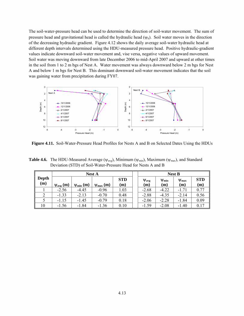
4.13

The soil-water-pressure head can be used to determine the direction of soil-water movement. The sum of pressure head and gravitational head is called the hydraulic head (ψh). Soil water moves in the direction of the decreasing hydraulic gradient. Figure 4.12 shows the daily average soil-water hydraulic head at different depth intervals determined using the HDU-measured pressure head. Positive hydraulic-gradient values indicate downward soil-water movement and, vise versa, negative values of upward movement. Soil water was moving downward from late December 2006 to mid-April 2007 and upward at other times in the soil from 1 to 2 m bgs of Nest A. Water movement was always downward below 2 m bgs for Nest A and below 1 m bgs for Nest B. This dominant downward soil-water movement indicates that the soil was gaining water from precipitation during FY07.

0

2

4

6

8

10

12-5 -4 -3 -2 -1 0

Pressure Head (m)

Dep

th (m

) 10/1/200612/1/20062/1/20074/1/20076/1/20078/1/2007

Nest A

0

2

4

6

8

10

12-5 -4 -3 -2 -1 0

Pressure Head (m)

Dep

th (m

) 10/1/200612/1/20062/1/20074/1/20076/1/20078/1/2007

Nest B

Figure 4.11. Soil-Water-Pressure Head Profiles for Nests A and B on Selected Dates Using the HDUs

Table 4.6. The HDU-Measured Average (ψavg), Minimum (ψmin), Maximum (ψmax), and Standard Deviation (STD) of Soil-Water-Pressure Head for Nests A and B

Nest A Nest B Depth

(m) ψavg (m) ψmin (m) ψmax (m) STD (m)

ψavg (m)

ψmin (m)

ψmax (m)

STD (m)

1 -2.56 -4.45 -0.96 1.03 -2.68 -4.22 -1.71 0.77 2 -1.33 -2.13 -0.70 0.48 -2.88 -4.35 -2.14 0.56 5 -1.15 -1.45 -0.79 0.18 -2.06 -2.28 -1.84 0.09

10 -1.56 -1.84 -1.36 0.10 -1.59 -2.08 -1.40 0.17

4.14

Date

-2

-1.5

-1

-0.5

0

0.5

1

1.5

2

2.5

3

10/01/06

10/31/06

11/30/06

12/30/06

01/29/07

02/28/07

03/30/07

04/29/07

05/29/07

06/28/07

07/28/07

08/27/07

09/26/07

Hyd

raul

ic G

radi

ent (

m)

Nest A

1-2 m

2-5 m5-10 m

Date

-2

-1.5

-1

-0.5

0

0.5

1

1.5

2

2.5

3

10/01/06

10/31/06

11/30/06

12/30/06

01/29/07

02/28/07

03/30/07

04/29/07

05/29/07

06/28/07

07/28/07

08/27/07

09/26/07

Hyd

raul

ic G

radi

ent (

m)

Nest B

2-5 m

5-10 m1-2 m

Figure 4.12. Daily Average Soil-Water Hydraulic Head at Different Depth Intervals Determined Using the Measurements of the HDUs

4.15

4.4 Soil-Water Flux In FY07, neither of the two drain gauges detected any drainage. However, this does not necessarily indicate zero soil-water flux, but only that the drain gauges may not be applicable for the T Farm soil under the local weather conditions. As discussed in Section 3.5, either the soil in the gauges has much higher retention properties than expected for a tank farm, or the design of the wick system is not working as expected.

4.5 Instrument Performance The instrument performance is assessed against the indicators given in Table 6.2 of the Monitoring Plan and is given in Table 4.7. The performances of all instruments except three of the HDUs were within the ranges of the performance. However, although three of the four HDUs in Nest A reported values larger (wetter) than the upper bound of the performance indicators, this does not indicate the malfunction of the instruments but very wet soil conditions (wetter than -1 m pressure head) and/or the uncertainty of the HDU calibration curve [Eq. (2.5)].

Table 4.7. Instrument Performance

Monitoring Method Monitoring Component Performance

Indicator Within the

Indicated Range? 0.75 ≤ SDR ≤ 1.25 Yes Neutron Moisture

Probe Soil-Water Content (θv) PSCSC ×±= 98.0 Yes Capacitance Probe Soil-Water Content (θv) 0 ≤ θv ≤ θs Yes Heat Dissipation Unit Soil-Water Pressure (ψ) -100 m ≤ ψ ≤ -1 m Yes and No (a)

Heat Dissipation Unit Soil Temperature (Tsoil) 0°C ≤ Tsoil ≤ 30°C Yes

Drain Gauge Annual Soil-Water Drainage (D) 0 ≤ D ≤ Pannual Yes

Rain Gauge Precipitation (P) Annual value is within ±50% HMS measured P

Yes

Thermister Air Temperature (Tair) Annual average is within ±5% HMS Tair

Yes

(a) All pressure-head measurements in Nest B were within the indicated range, while some values at 1, 2, and 5 m depth in Nest A were larger than -1 m as shown in Figure 4.10.

5.1

5.0 Summary and Recommendations

This section summarizes instrument functionality and results of measured soil-water conditions. It also presents recommendations for future monitoring activities.

5.1 System Functionality During FY07, the battery voltage at the meteorological station and instrument Nests A and B all remained above 12.5 V, denoting that the battery voltages were sufficient for the stations to remain functional. The air temperature at the T Tank Farm meteorological station and that measured at the HMS were very similar, supporting the functionality of the temperature sensor. Cumulative precipitation measured at the T Tank Farm was slightly less than that measured at the HMS. However, this difference is not significant enough to indicate failure of the rain gauge and instead may be attributed to differences in uneven precipitation distribution. The soil temperature as measured by the HDUs produced typical trends with depth and compared similarly to soil-temperature data reported by Hsieh et al. (1973) and indicated the normal function of the HDU sensors. The good agreement of air temperature, precipitation, and soil-temperature measurements indicates normal functionality of the vadose zone monitoring system.

5.2 Soil Water Conditions The CP measurements showed that the soil-water content at relatively shallow depths (e.g., 0.6 and 0.9 m) was increasing since October 2006 and reached the highest in early January 2007, followed by a slight decrease. Soil-water contents at the depths of 1.3 m and deeper were relatively stable during the whole monitoring period. The standard deviations of soil-water content variation were between 0.003 and 0.015 m3m-3, with smaller variations in deeper soil. The neutron-probe measurements show that the normalized neutron counts had relatively large variations in the soil above 5 ft (1.52 m) bgs and were stable in the deeper soil. The HDU at the 1.0-m depth showed increasing soil-water pressures in early January before they started decreasing. The peak values of the HDU-measured soil-water-pressure head at 2-m depth appeared in early April 2007 followed by a decrease. The HDUs at the 2.0-m depth showed increasing soil-water pressures from January to April or May 2007 before they started decreasing. The soil-water-pressure heads at 5- and 10-m depths were relatively stable. During FY07, the standard deviations of soil-water-pressure-head were between 0.09 and 1.03 m H2O-height, with generally smaller variations in deeper soil. The HDU measurements in combination with elevation showed that the soil water was moving downward from late December 2006 to mid-April 2007 and upward at other times in the soil from 1 to 2 m bgs of Nest A. Water movement was always downward below 2 m bgs for Nest A and below 1 m bgs for Nest B. The dominant downward moisture movement indicates that the soil was gaining water from precipitation in FY07. Generally, the CPs, neutron probes, and HDUs showed results that were consistent with the weather conditions. The soil above ~1 m bgs became wetter in the fall of 2006 and winter of 2007 (under wet and cool weather conditions), and drier in the spring and summer of 2007 (under dry and hot weather

5.2

conditions); the soil from ~1 to ~2 m bgs showed similar seasonal variation but within a smaller range; and the soil-water conditions below ~2 m bgs were relatively stable. The drain gauges did not detect soil-water flux in the T-Farm soil under the natural conditions in FY07. Considering that no drain gauges are installed in Nests C and D, which will be under the surface barrier once the barrier is emplaced, the fact that no water fluxes will be measured in Nests A and B will have no impact on the monitoring of the soil-water conditions under the barrier.

5.3 Recommendations Based on the instrument performance and data obtained, the following recommendations are given:

• Calibrate the neutron probes for the access tube used to quantify soil-water content. For the neutron-probe measurements, the original data were recorded as neutron counts per 16 seconds at each location of measurement. By calibrating the neutron probe, the measured neutron counts can then be converted into actual soil-water contents. This provides the added advantages that the soil-water contents can be compared with the CP-measured water contents, and the water storage in the soil profile can be calculated.

• Move the 60-cm-depth sensor of the CP in Nest A down by one scale (10 cm) so that the measurements are not affected by the sealing bentonite.

• Measure the soil-water retention and the unsaturated hydraulic conductivities of the T Farm backfill materials between 0 and 10 m (0 to 33 ft) bgs so that the HDU measurements can be used to estimate soil-water flux.

• Do not use the water-flux meters installed in the T Farm to estimate the natural recharge rate due to the higher-than-expected silt content.

6.1

6.0 References

Atlantic-Richfield Hanford Company (ARHCO). 1973. 241-T-106 Tank leak investigation. ARH_2874, Atlantic-Richfield Hanford Company, Richland, WA. Baumhardt RL, RJ Lascano, and SR Evett. 2000. “Soil material, temperature, and salinity effects on calibration of multisensor capacitance probes.” Soil Sci. Soc. Am. J. 64:1940–1946. Campbell Scientific, Inc. 2004. Model 107 Temperature Probe Instruction Manual. Logan, UT. CH2M HILL. 2006. 241-T Tank Farm Vadose Zone Instrumentation. CH2M HILL Engineering Change Notice, ECN-723963 R1, CH2M HILL Hanford Group, Inc., Richland, WA. CH2M HILL. 2007. 241-T Tank Farm Vadose Zone Instrumentation. CH2M HILL Engineering Change Notice, ECN-724716 R2, CH2M HILL Hanford Group, Inc., Richland, WA. Decagon Devices, Inc. 2006. Drain Gauge – Gee Passive Capillary Lysimeter User’s Manual Version 3.0. Pullman, WA. Evett,SR JA Tolk, and TA Howell. 2006. “Soil profile water content determination: sensor accuracy, axial response, calibration, temperature dependence, and precision.” Vadose Zone Journal 5:894–907. Flint AL, GS Campbell, KM Ellett, and C Calissendorff. 2002. “Calibration and temperature correction of heat dissipation matric potential sensors.” Soil Sci. Soc. Am. J. 66:1439-1445. Hsieh JJ, AE Reisenauer, and LE Brownell. 1973. A study of soil water potential and temperature in Hanford soils. BNWL-1712, Pacific Northwest National Laboratory, Richland, WA. McMahon WJ. 2007. “Performance simulation of an interim surface barrier over the 242-T-106 Tank release.” In: AE Bauer, Design Analysis for T-Farm Interim Surface Barrier (TISB), Appendix A, RPP-33431 Rev. 0, CH2M HILL Hanford Group, Inc., Richland, WA. Myers DA. 2005. Field Investigation Report for Waste Management Areas. RPR-23752, CH2M HILL Hanford Group, Richland, WA. Paltineanu IC, and JL Starr. 1997. “Real-time soil water dynamics using multisensor capacitance probes: laboratory calibration.” Soil Sci. Soc. Am. J. 61:1576-1585. Ross L. 2007. Tank Farm Plant Operating Procedure - Operate Model 503DR Hydroprobe Neutron Moisture Detection. TO-320-022, B-8. CH2M HILL Hanford Group, Richland, WA. Routson RC, WH Price, DJ Brown, and KR Fecht. 1979. High-level waste leakage from the 241-T-106 tank at Hanford. RHO-ST-14, Rockwell Hanford Operations, Richland, WA. Sentek Pty Ltd. 2001. Calibration of the Sentek Pty Ltd Soil Moisture Sensors. Stepney, Australia. Shiozawa S and GS Campbell. 1990. “Soil thermal conductivity.” Remote Sens. Rev. 5:301-310.

6.2

Zhang ZF, JM Keller, and CE Strickland. 2007. T Tank Farm Interim Surface Barrier Demonstration – Vadose Zone Monitoring Plan. PNNL-16538, Pacific Northwest National Laboratory, Richland, WA.

PNNL-17306

Distr. 1

Distribution List No. of Copies ONSITE 11 CH2M-HILL Group, Inc. C.D. Wittreich (5) E6-35 J.E. Field E6-35 F.M. Mann E6-35 D.A. Myers E6-35 N.L. Peters E6-35 H.A. Sydnor E6-35 W.J. McMahon E6-35 1 DOE Richland Operations Office R.W. Lober H6-60 1 Washington State Department of Ecology J. Caggiano H0-57 1 Fluor Hanford S.W. Petersen E6-44 1 Energy Solutions K.D. Reynolds G1-62 6 Pacific Northwest National Laboratory Z.F. Zhang K9-36 C.E. Strickland K9-36 M.J. Fayer K9-36 A.L. Ward K9-36 Information Release (2) K1-06