t-stress in orthotropic functionally graded materials: lekhnitskii and
TRANSCRIPT
International Journal of Fracture 126: 345–384, 2004.© 2004 Kluwer Academic Publishers. Printed in the Netherlands.
T-stress in orthotropic functionally graded materials: Lekhnitskiiand Stroh formalisms
JEONG-HO KIM and GLAUCIO H. PAULINO∗Department of Civil and Environmental Engineering, University of Illinois at Urbana-Champaign, NewmarkLaboratory, 205 North Mathews Avenue, Urbana, IL 61801, U.S.A.∗Corresponding Author (E-mail: [email protected]; Phone: (217)333-3817; Fax: (217)265-8041)
Received 18 November 2002; accepted in revised form 13 January 2004
Abstract. A new interaction integral formulation is developed for evaluating the elastic T-stress for mixed-modecrack problems with arbitrarily oriented straight or curved cracks in orthotropic nonhomogeneous materials. Thedevelopment includes both the Lekhnitskii and Stroh formalisms. The former is physical and relatively simple,and the latter is mathematically elegant. The gradation of orthotropic material properties is integrated into the ele-ment stiffness matrix using a “generalized isoparametric formulation” and (special) graded elements. The specifictypes of material gradation considered include exponential and hyperbolic-tangent functions, but micromechanicsmodels can also be considered within the scope of the present formulation. This paper investigates several fractureproblems to validate the proposed method and also provides numerical solutions, which can be used as benchmarkresults (e.g. investigation of fracture specimens). The accuracy of results is verified by comparison with analyticalsolutions.
Key words: functionally graded material (FGM), fracture mechanics, orthotropic materials, T-stress, interactionintegral, two-state integral, finite element method (FEM), generalized isoparametric formulation (GIF).
1. Introduction
The non-singular stress (T-stress) of the Williams’s eigenfunction expansion (Williams, 1957)influences crack growth under mixed-mode loading (Williams and Ewing, 1972; Ueda et al.,1983; Smith et al., 2001). Williams and Ewing (1972), and Ueda et al. (1983) performedexperiments on polymethyl-methacrylate (PMMA) with a slanted internal crack, and foundthat the elastic T-stress influences the crack initiation angle. Smith et al. (2001) revisited earlierexperimental results for brittle fracture of PMMA, and re-examined the role of the T-stress inbrittle materials. The T-stress also influences crack path stability for mode I loading with asmall imperfection (Cotterell and Rice, 1980).
The T-stress influences crack-tip constraint and toughness under plane strain conditions(see, for example, O’Dowd et al., 1995). Larsson and Carlson (1973) investigated the T-stress,and observed that it affects the size and shape of the plastic zone. Betegón and Hancock (1991)investigated the two-parameter (J -T ) characterization of elastic-plastic crack-tip fields. Duand Hancock (1991) investigated the effect of the T-stress on the small-scale yielding field inelastic perfectly-plastic materials. Furthermore, O’Dowd and Shih (1991) developed the J -Qtheory (Q is a hydrostatic stress parameter) and found that the Q-family provides a frameworkfor quantifying the evolution of constraint from small-scale yielding to full yielding condi-tions. They deduced a one-to-one correspondence between Q and T , which is valid in thecase where the applied load and geometry affect Q only through T . O’Dowd and Shih (1992)

346 J.-H. Kim and G.H. Paulino
Figure 1. Cross-section microscope of FGMs: (a) lamellar NiCrAlY-PSZ FGM processed by plasma spray tech-nique (Sampath et al., 1995); (b) columnar ZrO2 − Y2O3 thermal barrier coating with graded porosity processedby electron beam physical vapor deposition (Kaysser and Ilschner, 1995).
also showed that the J -Q theory allows toughness to be measured and utilized in engineeringapplications.
Several numerical methods have been used to evaluate the elastic T-stress. Leevers andRadon (1982) used a variational formulation. Cardew et al. (1985) and Kfouri (1986) usedthe path-independent J -integral in conjunction with the interaction integral for mode I crackproblems. Sladek et al. (1997) used the Betti-Rayleigh reciprocal theorem for mixed-modecrack problems. Recently Chen et al. (2001) investigated the T-stress under mode I loadingby means of both the Betti-Rayleigh reciprocal theorem and Eshelby’s energy momentumtensor (the path-independent J -integral) using the p-version finite element method (FEM),and addressed the accuracy of numerical computations. All the papers mentioned above areconcerned with the T-stress for an isotropic homogeneous material.
The T-stress has been also investigated for both anisotropic and orthotropic homogeneoussolids. Gao and Chiu (1992) investigated slightly curved or kinked cracks under mode I load-ing in orthotropic elastic solids by means of perturbation analysis, which is based on complexvariable representations of the Stroh formalism. They also investigated the effects of mode-mixity, material orthotropy, and the T-stress on the behavior of a nearly symmetric crack. Yangand Yuan (2000a) evaluated the elastic T-stress and higher-order coefficients in the crack-tipfields in an anisotropic elastic solid by means of path-independent integrals (J -integral andBetti-Rayleigh reciprocal theorem) and the Stroh formalism. Yang and Yuan (2000b) alsoinvestigated a kinked crack in an anisotropic elastic solid, and evaluated the T-stress, stressintensity factors and energy release rates at the main and kinked crack tips by using the integralequation method and the Stroh formalism. However, all of the above papers are concerned withhomogeneous materials.
Functionally graded materials (FGMs) possess nonhomogeneous properties. These ma-terials were introduced to benefit from ideal performance of its constituents, e.g. heat andcorrosion resistance of ceramics together with mechanical strength and toughness of metals(Illshner, 1996). The books by Suresh and Mortensen (1998) and Miyamoto et al. (1999), andthe review chapter by Paulino et al. (2003) present comprehensive information about various
Lekhnitskii and Stroh formalisms 347
aspects of FGMs. Such materials may exhibit isotropic or orthotropic material properties de-pending on processing techniques. For instance, large-size bulk FGMs fabricated by the sparkplasma sintering (SPS) technique may be modeled as isotropic materials (Tokita, 1999). Onthe other hand, graded materials processed by plasma spray techniques may have a lamellarstructure (Sampath et al., 1995) (see Figure 1a), while materials processed by electron beamphysical vapor deposition (PVD) may have a columnar structure (Kaysser and Ilschner, 1995)(see Figure 1b). Thus, an isotropic FGM model can be used for materials fabricated by SPS,and an orthotropic FGM model for materials fabricated by plasma spraying or PVD.
The T-stress has been investigated for isotropic FGMs. Becker et al. (2001) investigatedthe T-stress and finite crack kinking, and found that the T-stress in FGMs depends on both thefar-field loading and the far-field phase angle (ψ∞ = tan−1(σ∞
xy /σ∞yy )), and that the magnitude
of T-stress in the FGMs investigated was, on average, greater than that for homogeneous ma-terials with identical geometry. They calculated the T-stress using the difference of the normalstresses along θ = 0, i.e. (σxx − σyy), which is a method that can lead to significant numericalerrors due to the recovery of stresses very close to the crack tip. Recently, Kim and Paulino(2003d) proposed a unified approach using the interaction integral method to evaluate T-stressand SIFs, and also investigated the effect of T-stress on the crack initiation angle. In addition,Paulino and Kim (2004) evaluated the T-stress in isotropic FGMs using a non-equilibriumformulation of the interaction integral method, and provided some benchmark solutions forthe T-stress and the biaxiality ratio considering graded laboratory fracture specimens. Noticethat the papers by Kim and Paulino (2003d) and Paulino and Kim (2004) focus on isotropicFGMs, while the present one focuses on orthotropic FGMs.
The contribution of this paper consists of evaluating the T-stress in orthotropic FGMsby means of the interaction integral method in conjunction with the Lekhnitskii and Strohformalisms. Based on the assumption that the graded orthotropic material is locally homogen-eous near the crack tip, with continuous, differentiable and bounded material properties, thispaper establishes the relationship between the asymptotically defined interaction integral (M-integral) and the T-stress, converts the M-integral to an equivalent domain integral (EDI) usingauxiliary fields, and calculates the T-stress using a finite domain. This paper builds upon theearlier work by Kim and Paulino (2003b), which focuses on the interaction integral method toevaluate mixed-mode stress intensity factors (SIFs) in orthotropic FGMs.
In this paper, we employ two equivalent formalisms: Lekhnitskii and Stroh, to obtain theauxiliary fields for the T-stress in orthotropic FGMs. The two formalisms treat plane problemsin an anisotropic elastic body. While the Lekhnitskii formalism assumes that stress fieldsdepend on plane coordinates, the Stroh formalism assumes that displacement fields dependon plane coordinates. Barnett and Kirchner (1997) provided a direct and straightforwardproof of the equivalence between the Lekhnitskii and Stroh formalisms by reducing the six-dimensional form of Stroh’s formalism to two homogeneous linear equations, which involvereduced elastic compliances of the Lekhnitskii formalism.
This paper is organized as follows. Section 2 reviews anisotropic elasticity. Section 3presents the crack-tip fields in anisotropic materials, and Section 4 provides auxiliary fieldschosen for the T-stress in the interaction integral method. Section 5 explains the theoreticalformulation, and establishes the relationship between the M-integral and the T-stress. Sec-tion 6 presents numerical aspects of the M-integral, and various features of the finite elementimplementation. Section 7 presents various numerical examples. Finally, Section 8 concludesthe work.

348 J.-H. Kim and G.H. Paulino
2. Anisotropic elasticity
The generalized Hooke’s law relating stress to strain is given by (Lekhnitskii, 1968)
εi = aij σj , aij = aji (i, j = 1, 2, . . . , 6), (1)
where the compliance coefficients, aij , are contracted notations of the compliance tensor Sijkl
and the following notation is used
ε1 = ε11, ε2 = ε22, ε3 = ε33, ε4 = 2ε23, ε5 = 2ε13, ε6 = 2ε12
σ1 = σ11, σ2 = σ22, σ3 = σ33, σ4 = σ23, σ5 = σ13, σ6 = σ12.(2)
For plane stress, the aij components of interest are
aij (i, j = 1, 2, 6) (3)
and for plane strain, aij are exchanged with bij as follows:
bij = aij − ai3aj3
a33(i, j = 1, 2, 6). (4)
Two dimensional anisotropic elasticity problems can be formulated in terms of the analyticfunctions, φk(zk), of the complex variable, zk = xk + iyk (k = 1, 2), i = √−1, where
xk = x + αky, yk = βky, (k = 1, 2). (5)
The parameters αk and βk are the real and imaginary parts of µk = αk + iβk, which can bedetermined from the following characteristic equation (Lekhnitskii, 1968)
a11µ4 − 2a16µ
3 + (2a12 + a66)µ2 − 2a26µ + a22 = 0, (6)
where the roots µk are always complex or purely imaginary in conjugate pairs as µ1, µ1; µ2,µ2.
3. Crack-tip fields: actual fields
Figure 2 shows Cartesian and polar coordinate systems originating at a crack tip in an ortho-tropic FGM. The asymptotic stress and displacement fields are given by (see Sih et al. (1965)for the homogeneous case)

Lekhnitskii and Stroh formalisms 349
Figure 2. Cartesian (x1, x2) and polar (r, θ) coordinates originating from a crack tip in an orthotropic nonhomo-geneous material under traction (t) and displacement boundary conditions.
σ11 = KI√2πr
Re
µ
tip1 µ
tip2
µtip1 − µ
tip2
µ
tip2√
cos θ + µtip2 sin θ
− µtip1√
cos θ + µtip1 sin θ
+ KII√2πr
Re
1
µtip1 − µ
tip2
(µ
tip2 )2√
cos θ + µtip2 sin θ
− (µtip1 )2√
cos θ + µtip1 sin θ
+ T ,
σ22 = KI√2πr
Re
1
µtip1 − µ
tip2
µ
tip1√
cos θ + µtip2 sin θ
− µtip2√
cos θ + µtip1 sin θ
+ KII√2πr
Re
1
µtip1 − µ
tip2
1√
cos θ + µtip2 sin θ
− 1√cos θ + µ
tip1 sin θ
,
σ12 = KI√2πr
Re
µ
tip1 µ
tip2
µtip1 − µ
tip2
1√
cos θ + µtip1 sin θ
− 1√cos θ + µ
tip2 sin θ
+ KII√2πr
Re
1
µtip1 − µ
tip2
µ
tip1√
cos θ + µtip1 sin θ
− µtip2√
cos θ + µtip2 sin θ
,
(7)
and

350 J.-H. Kim and G.H. Paulino
u1 = KI
√2r
πRe
[1
µtip1 −µ
tip2
{µ
tip1 p
tip2
√cos θ+µ
tip2 sin θ−µ
tip2 p
tip1
√cos θ+µ
tip1 sin θ
}]
+ KII
√2r
πRe
[1
µtip1 −µ
tip2
{p
tip2
√cos θ+µ
tip2 sin θ−p
tip1
√cos θ+µ
tip1 sin θ
}]+a
tip11T r cos θ,
u2 = KI
√2r
πRe
[1
µtip1 −µ
tip2
{µ
tip1 q
tip2
√cos θ+µ
tip2 sin θ−µ
tip2 q
tip1
√cos θ+µ
tip1 sin θ
}]
+ KII
√2r
πRe
[1
µtip1 −µ
tip2
{q
tip2
√cos θ+µ
tip2 sin θ−q
tip1
√cos θ+µ
tip1 sin θ
}]+a
tip12T r sin θ,
(8)
respectively, where T denotes the elastic T-stress, atip11 and a
tip12 denote material parameters
evaluated at the crack tip, Re denotes the real part of the complex function, and µtip1 and µ
tip2
denote crack-tip material parameters evaluated by means of Equation (6), which are taken forβk > 0 (k = 1, 2), and p
tipk and q
tipk are given by
ptipk = a
tip11 (µ
tipk )2 + a
tip12 − a
tip16µ
tipk ,
qtipk = a
tip12µ
tipk + a
tip22
µtipk
− atip26 ,
(9)
respectively. Notice that in the above expressions, the material parameters are sampled atthe crack-tip location, which is the main difference from the expressions for homogeneousmaterials (Sih et al., 1965).
4. Auxiliary fields
Auxiliary fields are secondary field solutions. Superposition of auxiliary and actual fieldsleads to the relationship between the interaction integral and the target solution (T-stress). Theauxiliary fields involve stresses (σ aux), strains (εaux) and displacements (uaux). In this paper,we adopt fields (stresses and displacements) originally developed for homogeneous materialsand use a formulation (Kim and Paulino, 2003a, 2003d) which accounts for the displacementmismatch between the homogeneous and graded materials.
4.1. STRESS AND DISPLACEMENT FIELDS
To evaluate the T-stress, we use the auxiliary fields associated with a point force applied to thecrack tip of a semi-infinite crack in an infinite homogeneous orthotropic body in a directionparallel to the crack surface, as illustrated in Figure 3. The material orthotropy directions arealigned with the global coordinates. The auxiliary fields are derived by means of the equivalentLekhnitskii and Stroh formalisms, which are explained below (see also Kim (2003)).
4.1.1. Lekhnitskii FormalismThe Lekhnitskii formalism generalizes the Muskhelishvili approach (Muskhelishvili, 1933)for two-dimensional deformation of an anisotropic elastic body, and begins with stresses byassuming that they only depend on plane coordinates. Details are explained in the book by

Lekhnitskii and Stroh formalisms 351
Figure 3. A point force applied at the crack tip in the direction parallel to the crack surface in a homogeneousorthotropic body where material orthotropy directions are aligned with the global coordinates.
Ting (1996). In the Lekhnitskii formalism, we use the known auxiliary stress fields, anddetermine derivatives of auxiliary displacements. The auxiliary stresses, with respect to thepolar coordinates (r, φ), are given as (Lekhnitskii, 1968):
σ auxrr = A cos φ + B sin φ
rF (φ), σ aux
φφ = σ auxrφ = 0, (10)
where
F (φ) = atip11 cos4 φ + (2a
tip12 + a
tip66 ) sin2 φ cos2 φ + a
tip22 sin4 φ (11)
and the material parameters aij ≡ atipij are evaluated at the crack tip location, which differ
from a homogeneous material (Lekhnitskii, 1968). The constants A and B are determinedfrom equilibrium conditions for a semi-infinite crack in an infinite homogeneous orthotropicbody as shown in Figure 3. The equilibrium equations with respect to the global Cartesiancoordinates, i.e. X1 and X2, are (Lekhnitskii, 1968)
A
∫ ψ2
−ψ1
cos2 φ
F (φ)dφ + B
∫ ψ2
−ψ1
sin φ cos φ
F (φ)dφ = −f cos ω,
A
∫ ψ2
−ψ1
sin φ cos φ
F (φ)dφ + B
∫ ψ2
−ψ1
sin2 φ
F (φ)dφ = −f sin ω.
(12)
The auxiliary stresses with respect to the global coordinates are given by
σ aux11 = A cos φ + B sin φ
rF (φ)cos2 φ,
σ aux22 = A cos φ + B sin φ
rF (φ)sin2 φ,
σ aux12 = A cos φ + B sin φ
rF (φ)sin φ cos φ.
(13)

352 J.-H. Kim and G.H. Paulino
Using the stress-strain and strain-displacement relationships, one obtains displacement deriv-atives with respect to the global Cartesian coordinates as follows:
u1,1 = (atip11 cos2 φ + a
tip12 sin2 φ)
A cos φ + B sin φ
rF (φ),
u2,2 = (atip12 cos2 φ + a
tip22 sin2 φ)
A cos φ + B sin φ
rF (φ),
u1,2 = 1
rF (φ){A sin φF (φ) − AH1(φ) − BH2(φ)},
u2,1 = 1
rF (φ)[2a
tip66 (A cos φ+B sin φ) sin φ cos φ − {A sin φF (φ)−AH1(φ)−BH2(φ)}],
(14)
where
H1(φ) = atip11 cos4 φ sin φ+a
tip12 sin φ cos2 φ−a
tip22 sin3 φ cos2 φ−(2a
tip12 +a
tip66 ) sin φ cos4 φ,
H2(φ) = atip11 cos3 φ + a
tip12 sin2 φ cos φ. (15)
The actual derivation of Equation (14) is given in Appendix A.
4.1.2. Stroh FormalismThe Stroh formalism considers two-dimensional deformation of an anisotropic elastic body,and starts with displacements by assuming that they only depend on plane coordinates. Detailsare explained in the book by Ting (1996). In the Stroh formalism, the auxiliary displacementswith respect to the local coordinates (x1, x2) are given by (Ting, 1996):
uaux = −1
2
[1
πln rI + S(θ)
]h, (16)
where uaux=[uaux1 , uaux
2 ]T , I denotes the identity matrix, and S(θ) and h are given by
S(θ) = 2
πRe [A C(θ) BT ],
h = L−1f ,
(17)
where
A =[
λtip1 p
tip1 λ
tip2 p
tip2
λtip1 q
tip1 λ
tip2 q
tip2
], B =
[ −λtip1 µ
tip1 −λ
tip2 µ
tip2
λtip1 λ
tip2
],
C(θ) =[
ln s1(θ) 0
0 ln s2(θ)
], sk(θ) = cos θ + µ
tipk sin θ,
L−1 = Re [iAB−1], f = [f, 0]T ,
(18)
in which ptipk and q
tipk (k = 1, 2) are given by Equation (9), and λ
tipk (k = 1, 2) is the
normalization factor given by the following expression
2(λtipk )2(q
tipk /µ
tipk − µ
tipk p
tipk ) = 1. (19)
The auxiliary stresses, with respect to the local Cartesian coordinates (x1, x2), are givenby (Ting, 1996) (k = 1, 2):

Lekhnitskii and Stroh formalisms 353
Figure 4. Illustration of the ‘incompatibility formulation’ accounting for material nonhomogeneity. Notice that S
(x) �= St ip for x �= 0. The area A denotes a representative region around the crack tip.
σ auxrr = 1
2πrnT (θ)N3(θ)h, σ aux
θθ = σ auxrθ = 0, (20)
where
n = [cos θ, sin θ]T , N3(θ) = 2Re [B P (θ) BT ]
P (θ) =[
µ1(θ) 0
0 µ2(θ)
], µk(θ) = µ
tipk cos θ − sin θ
µtipk sin θ + cos θ
.
(21)
In Equations (16) to (21), material parameters are evaluated at the crack tip location, whichdiffers from a homogeneous material (Yang and Yuan, 2000a). Further details of the Strohformalism are given in Appendix B.
4.2. STRAIN FIELD
In this paper, we use an ‘incompatibility formulation’ that involves the auxiliary strain fieldgiven by
εauxij = Sijkl(x) σ aux
kl , (22)
where Sijkl(x) is the compliance tensor of FGMs and Sijkl(x) �= Sijkl(tip) for x �= 0 as shownin Figure 4. Notice that, in this case, the auxiliary stress fields in Equations (10) and (20) are inequilibrium, i.e. σ aux
ij,j = 0 (no body forces), however, the auxiliary strain field in Equation (22)is not compatible with the auxiliary displacement field, i.e. εaux
ij �= (uauxi,j + uaux
j,i )/2. Thisincompatibility must be considered in the interaction integral formulation. The formulationwas first proposed by Dolbow and Gosz (2002) to evaluate SIFs for nonhomogeneous isotropicmaterials.
Alternative formulations, using the auxiliary fields for homogeneous orthotropic materials(see previous subsections), can also be developed. For instance, one can use compatible dis-placements and strains, and a constant constitutive tensor around the crack tip. This choice

354 J.-H. Kim and G.H. Paulino
Figure 5. Conversion of the contour integral into an equivalent domain integral (EDI) where� = �o + �+ − �s + �−, mj = nj on �o and mj = −nj on �s .
of auxiliary fields violates the stress-strain relationship in FGMs, while it satisfies compat-ibility and equilibrium. Another alternative is to use compatible displacements and strains,and the actual constitutive tensor of FGMs. This formulation violates equilibrium, while itsatisfies compatibility and the stress-strain relationship. This ‘non-equilibrium formulation’was proposed by Paulino and Kim (2004) to evaluate the T-stress in isotropic FGMs.
5. The interaction integral: M-integral
The interaction integral is derived from the path-independent J -integral (Rice, 1968) for twoadmissible states of a cracked elastic orthotropic FGM. Therefore, the interaction integral(M-integral1 ) is a two-state integral. For the sake of numerical efficiency, the interactionintegral employs an equivalent domain integral (EDI) (Raju and Shivakumar, 1990) form.The theoretical formulation, extraction of T-stress, and numerical aspects are provided below.
5.1. M-INTEGRAL: FORMULATION
The standard J -integral (Rice, 1968) is given by
J = lim�s→0
∫�s
(Wδ1j − σij ui,1) nj d�, (23)
where W is the strain energy density expressed by
W = 1
2σij εij = 1
2Cijklεklεij , (24)
1Here, the so-called M-integral should not be confused with the M-integral (conservation integral) of Knowlesand Sternberg (1972), Budiansky and Rice (1973), and Chang and Chien (2002). Also, see the book by Kanninenand Popelar (1985) for a review of conservation integrals in fracture mechanics.

Lekhnitskii and Stroh formalisms 355
Figure 6. Plateau weight function (q-function).
and nj is the outward normal vector to the contour �s , as shown in Figure 5. To convert thecontour integral into an EDI, the following contour integral is defined:
H =∮
�
(Wδ1j − σij ui,1) mjq d�, (25)
where �=�o +�+−�s +�−, mj is a unit vector outward normal to the corresponding contour(i.e. mj=nj on �o and mj=-nj on �s), and q is an admissible weight function varying fromq = 1 on �s to q = 0 on �o (see Figure 6). Taking the limit �s → 0 leads to
lim�s→0
H = lim�s→0
∮�
(Wδ1j − σij ui,1) mjq d�
= lim�s→0
∫�o+�++�−−�s
(Wδ1j −σij ui,1) mjq d�
= lim�s→0
[∫�o+�++�−
(Wδ1j −σij ui,1) mjq d�+∫
−�s
(Wδ1j −σij ui,1) mjq d�
]
= lim�s→0
[∫�o+�++�−
(Wδ1j −σij ui,1) mjq d�−∫
�s
(Wδ1j −σij ui,1) njq d�
].
(26)
Because q = 0 on �o and the crack faces are assumed to be traction-free, one obtains
J = − lim�s→0
H = − lim�s→0
∮�
(Wδ1j − σij ui,1) mjq d�. (27)
Applying the divergence theorem to Equation (27) and using the weight function q, oneobtains the EDI as
J =∫
A
(σij ui,1 − Wδ1j ) q,j dA +∫
A
(σij ui,1 − Wδ1j ),j q dA. (28)
356 J.-H. Kim and G.H. Paulino
The J -integral of the superimposed fields (actual and auxiliary fields) is given as:
J s =∫
A
{(σij + σ aux
ij ) (ui,1 + uauxi,1 ) − 1
2(σik + σ aux
ik )(εik + εauxik )δ1j
}q,j dA
+∫
A
{(σij + σ aux
ij ) (ui,1 + uauxi,1 ) − 1
2(σik + σ aux
ik )(εik + εauxik )δ1j )
},j
q dA,
(29)
which is conveniently decomposed into
J s = J + J aux + M , (30)
where J aux is given by
J aux =∫
A
(σ auxij uaux
i,1 − W auxδ1j ) q,j dA +∫
A
{σ aux
ij uauxi,1 − 1
2σ aux
ik εauxik δ1j
},j
q dA, (31)
and the resulting general form of the interaction integral (M) is given by
M =∫
A
{σiju
auxi,1 + σ aux
ij ui,1 − 1
2(σikε
auxik + σ aux
ik εik)δ1j
}q,jdA
+∫
A
{σiju
auxi,1 + σ aux
ij ui,1 − 1
2(σikε
auxik + σ aux
ik εik)δ1j
},j
q dA.
(32)
The specific interaction integral (M), based on the incompatibility formulation, is derived asfollows. Using the following identity
σij εauxij = σijCijkl(x)σ aux
kl = σ auxkl εkl = σ aux
ij εij , (33)
one rewrites Equation (32) as
M =∫
A
{σiju
auxi,1 + σ aux
ij ui,1 − σikεauxik δ1j
}q,jdA
+∫
A
{σiju
auxi,1 + σ aux
ij ui,1 − σikεauxik δ1j
},j
q dA
= M1 + M2.
(34)
Moreover, the last term of the second integral (M2) in Equation (34) is expressed as
(σikεauxik δ1j ),j = (σij ε
auxij ),1 = (Cijklεklε
auxij ),1
= Cijkl,1εklεauxij + Cijklεkl,1ε
auxij + Cijklεklε
auxij,1
= Cijkl,1εklεauxij + σ aux
ij εij,1 + σij εauxij,1 .
(35)
Substitution of Equation (35) into M2 in Equation (34) leads to
M2 =∫
A
(σij,j u
auxi,1 + σiju
auxi,1j + σ aux
ij,j ui,1 + σ auxij ui,1j ) q dA
−∫
A
(Cijkl,1εklεauxij + σ aux
ij εij,1 + σij εauxij,1
)q dA.
(36)
Using equilibrium (actual and auxiliary) and compatibility (actual), one simplifies M2 inEquation (36) as

Lekhnitskii and Stroh formalisms 357
M2 =∫
A
{σij (u
auxi,1j − εaux
ij,1 ) − Cijkl,1εklεauxij
}q dA.
Therefore the resulting interaction integral (M) becomes
M =∫
A
{σiju
auxi,1 + σ aux
ij ui,1 − σikεauxik δ1j
}q,jdA
+∫
A
{σij (u
auxi,1j − εaux
ij,1 ) − Cijkl,1εklεauxij
}q dA,
(37)
where the underlined term is an incompatible term, which appears due to incompatibility ofthe auxiliary strain fields. The incompatibility formulation for the extraction of mixed-modeSIFs in isotropic FGMs was first developed by Dolbow and Gosz (2002).
5.2. M-INTEGRAL: THE EXISTENCE OF THE M-INTEGRAL FOR FGMS
The existence of the integral in Equation (37) as r goes to zero is proved below. The termσij ε
auxij,1 in Equation (37) can be written as
σij εauxij,1 = σij {Sijkl,1(x) σ aux
kl + Sijkl(x) σ auxkl,1 }
= σij (Sijkl)tip σ auxkl,1 + σijSijkl,1(x) σ aux
kl + σij (Sijkl(x) − (Sijkl)tip) σ auxkl,1
= σijuauxi,1j + σijSijkl,1(x) σ aux
kl + σij (Sijkl(x) − (Sijkl)tip) σ auxkl,1 .
(38)
Thus
σij (uauxi,1j − εaux
ij,1 ) = −σijSijkl,1(x) σ auxkl − σij (Sijkl(x) − (Sijkl)tip) σ aux
kl,1 , (39)
where the first term of the right hand expression vanishes as r goes to zero because of smooth-ness assumption of the constitutive tensor, and we focus on the underlined term. The compli-ance tensor involving material properties must be continuous and differentiable function, andthus it can be written as (Eischen, 1987)
Sijkl(r, θ) = (Sijkl)t ip + rS(1)ijkl (θ) + r2
2S
(2)ijkl(θ) + O(r3) + . . ., (40)
where S(n)ijkl(θ) (n = 1, 2, . . .) are angular functions. For the auxiliary fields for T-stress
(uaux = O(ln r), σ aux = O(r−1)), the integral, as the limit r goes to zero, becomes
limA→0
∫A
σij (uauxi,1j − εaux
ij,1 ) q dA = limr→0
∫θ
∫r
σij (uauxi,1j − εaux
ij,1 )qrdrdθ
= − limr→0
∫θ
∫r
σij (Sijkl(r, θ)−(Sijkl)t ip)σ auxkl,1 qrdrdθ
= − limr→0
∫θ
∫r
O(r−1/2)O(r)O(r−2)qrdrdθ
= − limr→0 O(r1/2) = 0.
(41)
The integral involving material derivatives (Cijkl,1) in Equation (37) vanishes for the fol-lowing reason. Derivatives of the elastic moduli are assumed to be bounded at the crack tip,i.e. Cijkl,1 is O(rα) with α ≥ 0. Therefore, as the limit r goes to zero, the integral becomes
358 J.-H. Kim and G.H. Paulino
limA→0
∫A
Cijkl,1εklεauxij qdA = lim
r→0
∫θ
∫r
Cijkl,1 εkl εauxij q rdrdθ
= limr→0
∫θ
∫r
O(rα)O(r−1/2)O(r−1) q r dr dθ
= limr→0
O(rα+1/2) = 0.
(42)
Thus the limit exists and the proposed integral is well-posed.
5.3. M-INTEGRAL: EXTRACTION OF THE T-STRESS
The procedure for extracting the T-stress in orthotropic FGMs is the same as that for isotropicFGMs, which is explained in detail by Kim and Paulino (2003a) and Paulino and Kim (2004).The T-stress can be extracted from the interaction integral taking the limit r → 0 of thedomain A shown in Figure 5. By doing so, the contributions of the higher-order (i.e. O(r1/2)
and higher) and singular (i.e. O(r−1/2)) terms vanish.Equation (32) is rewritten as
Mlocal =∫
A
[{(σij u
auxi,1 + σ aux
ij ui,1) − 1
2(σikε
auxik + σ aux
ik εik)δ1j
}q
],j
dA, (43)
where Mlocal denotes the M-integral with respect to local coordinates (x1, x2) (see Figure 5).By applying the divergence theorem to Equation (43), one obtains
Mlocal = lim�s→0
∮�
{(σij u
auxi,1 + σ aux
ij ui,1) − 1
2(σikε
auxik + σ aux
ik εik)δ1j
}mjq d�. (44)
Because mj=-nj and q = 1 on �s , mj=nj and q = 0 on �o, and the crack faces are assumedto be traction-free, then Equation (44) becomes
Mlocal = lim�s→0
∫�s
[1
2(σikε
auxik + σ aux
ik εik)δ1j − (σij uauxi,1 + σ aux
ij ui,1)
]nj d�. (45)
Using the equality in Equation (33), one reduces Equation (45) to
Mlocal = lim�s→0
∫�s
[σikε
auxik δ1j − (σiju
auxi,1 + σ aux
ij ui,1)]nj d�. (46)
The actual stress fields are given by
σij = KI(2πr)−1/2f Iij (θ, µ
tip1 , µ
tip2 ) + KII (2πr)−1/2f II
ij (θ, µtip1 , µ
tip2 ) + T δ1iδ1j + O(r1/2),
(47)
where the functions f Iij (θ, µ
tip1 , µ
tip2 ) and f II
ij (θ, µtip1 , µ
tip2 ) (i, j = 1,2) are given in Equa-
tion (7). As the contour �s (see Figure 5) shrinks to the crack tip region, the higher-order termscancel out as mentioned above. Moreover, there is no contribution from the singular termsO(r−1/2) because the integrations from θ = −π to +π of angular functions (coefficients) ofthe three terms given in Equation (46) are cancelled out, and become zero regardless of theresulting singularity O(r−1/2).
According to the above argument, the only term that contributes to M is the term involvingT . Thus we can consider only the stress parallel to the crack direction:
Lekhnitskii and Stroh formalisms 359
σij = T δ1iδ1j . (48)
Substituting Equation (48) into Equation (46), one obtains
Mlocal = − lim�s→0
∫�s
σ auxij njui,1 d� = T a
tip11 lim
�s→0
∫�s
σ auxij nj d�. (49)
Because the force f is in equilibrium (see Figure 3)
f = − lim�s→0
∫�s
σ auxij nj d�, (50)
and thus the following simple and important relationship is obtained
T = Mlocal
f atip11
, (51)
where atip11 is a material parameter at the crack tip location based on the local coordinates for
plane stress, and is replaced by btip11 for plane strain (cf. Equation (4)). For isotropic materials,
Equation (51) becomes
T = E∗tip
fMlocal, (52)
where E∗tip = Etip for plane stress and Etip/(1 − ν2
tip) for plane strain.
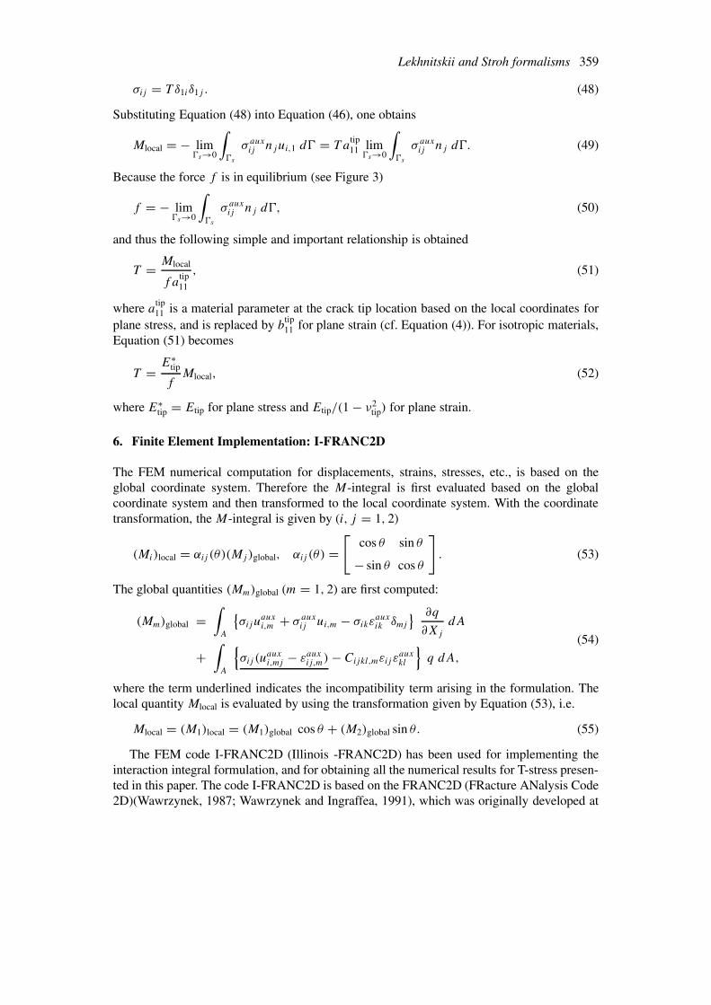
6. Finite Element Implementation: I-FRANC2D
The FEM numerical computation for displacements, strains, stresses, etc., is based on theglobal coordinate system. Therefore the M-integral is first evaluated based on the globalcoordinate system and then transformed to the local coordinate system. With the coordinatetransformation, the M-integral is given by (i, j = 1, 2)
(Mi)local = αij (θ)(Mj )global, αij (θ) =[
cos θ sin θ
− sin θ cos θ
]. (53)
The global quantities (Mm)global (m = 1, 2) are first computed:
(Mm)global =∫
A
{σiju
auxi,m + σ aux
ij ui,m − σikεauxik δmj
} ∂q
∂Xj
dA
+∫
A
{σij (u
auxi,mj − εaux
ij,m) − Cijkl,mεij εauxkl
}q dA,
(54)
where the term underlined indicates the incompatibility term arising in the formulation. Thelocal quantity Mlocal is evaluated by using the transformation given by Equation (53), i.e.
Mlocal = (M1)local = (M1)global cos θ + (M2)global sin θ. (55)
The FEM code I-FRANC2D (Illinois -FRANC2D) has been used for implementing theinteraction integral formulation, and for obtaining all the numerical results for T-stress presen-ted in this paper. The code I-FRANC2D is based on the FRANC2D (FRacture ANalysis Code2D)(Wawrzynek, 1987; Wawrzynek and Ingraffea, 1991), which was originally developed at
360 J.-H. Kim and G.H. Paulino
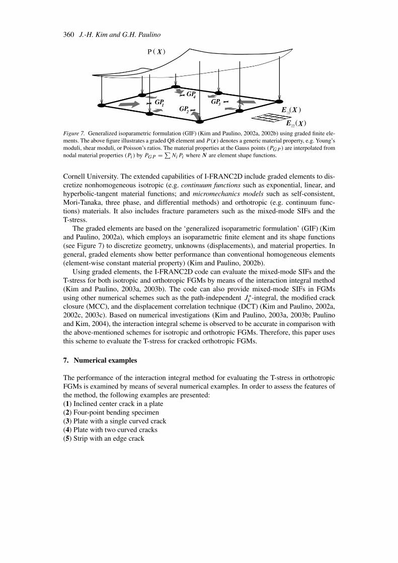
Figure 7. Generalized isoparametric formulation (GIF) (Kim and Paulino, 2002a, 2002b) using graded finite ele-ments. The above figure illustrates a graded Q8 element and P(x) denotes a generic material property, e.g. Young’smoduli, shear moduli, or Poisson’s ratios. The material properties at the Gauss points (PGP ) are interpolated fromnodal material properties (Pi ) by PGP = ∑
NiPi where N are element shape functions.
Cornell University. The extended capabilities of I-FRANC2D include graded elements to dis-cretize nonhomogeneous isotropic (e.g. continuum functions such as exponential, linear, andhyperbolic-tangent material functions; and micromechanics models such as self-consistent,Mori-Tanaka, three phase, and differential methods) and orthotropic (e.g. continuum func-tions) materials. It also includes fracture parameters such as the mixed-mode SIFs and theT-stress.
The graded elements are based on the ‘generalized isoparametric formulation’ (GIF) (Kimand Paulino, 2002a), which employs an isoparametric finite element and its shape functions(see Figure 7) to discretize geometry, unknowns (displacements), and material properties. Ingeneral, graded elements show better performance than conventional homogeneous elements(element-wise constant material property) (Kim and Paulino, 2002b).
Using graded elements, the I-FRANC2D code can evaluate the mixed-mode SIFs and theT-stress for both isotropic and orthotropic FGMs by means of the interaction integral method(Kim and Paulino, 2003a, 2003b). The code can also provide mixed-mode SIFs in FGMsusing other numerical schemes such as the path-independent J ∗
k -integral, the modified crackclosure (MCC), and the displacement correlation technique (DCT) (Kim and Paulino, 2002a,2002c, 2003c). Based on numerical investigations (Kim and Paulino, 2003a, 2003b; Paulinoand Kim, 2004), the interaction integral scheme is observed to be accurate in comparison withthe above-mentioned schemes for isotropic and orthotropic FGMs. Therefore, this paper usesthis scheme to evaluate the T-stress for cracked orthotropic FGMs.
7. Numerical examples
The performance of the interaction integral method for evaluating the T-stress in orthotropicFGMs is examined by means of several numerical examples. In order to assess the features ofthe method, the following examples are presented:(1) Inclined center crack in a plate(2) Four-point bending specimen(3) Plate with a single curved crack(4) Plate with two curved cracks(5) Strip with an edge crack
Lekhnitskii and Stroh formalisms 361
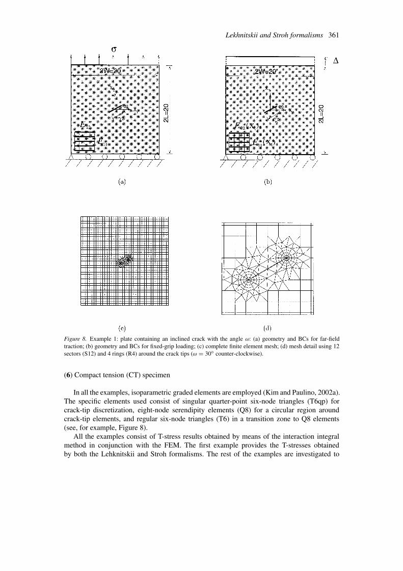
Figure 8. Example 1: plate containing an inclined crack with the angle ω: (a) geometry and BCs for far-fieldtraction; (b) geometry and BCs for fixed-grip loading; (c) complete finite element mesh; (d) mesh detail using 12sectors (S12) and 4 rings (R4) around the crack tips (ω = 30◦ counter-clockwise).
(6) Compact tension (CT) specimen
In all the examples, isoparametric graded elements are employed (Kim and Paulino, 2002a).The specific elements used consist of singular quarter-point six-node triangles (T6qp) forcrack-tip discretization, eight-node serendipity elements (Q8) for a circular region aroundcrack-tip elements, and regular six-node triangles (T6) in a transition zone to Q8 elements(see, for example, Figure 8).
All the examples consist of T-stress results obtained by means of the interaction integralmethod in conjunction with the FEM. The first example provides the T-stresses obtainedby both the Lehknitskii and Stroh formalisms. The rest of the examples are investigated to

362 J.-H. Kim and G.H. Paulino
evaluate the T-stress by means of the Lehknitskii formalism. In order to validate T-stresssolutions, the first example includes analytical closed-form solutions for an orthotropic ho-mogeneous material, and is investigated for an inclined center crack in a plate (a/W = 0.1),which approximates an infinite domain. The same example is investigated for an FGM plateunder fixed-grip loading considering exponentially graded material properties. The secondexample involves a four-point bending specimen with a delamination crack. The third andfourth examples investigate the effect of curved crack(s) in a plate, which naturally involvesmode mixity. These two examples allow one to evaluate the effect of crack curvature andmultiple cracks on the T-stress. The fifth example investigates an edge crack in a strip con-sidering hyperbolic-tangent material functions, and investigates the effect of translation ofthe material properties. The last example investigates a compact tension (CT) specimen andprovides numerical solutions for the T-stress and the biaxiality ratio considering exponentiallygraded materials.
7.1. INCLINED CENTER CRACK IN A PLATE
Figures 8a and 8b show an inclined center crack of length 2a located with a geometric angle ω
(counter-clockwise) in a plate under far-field constant traction and fixed-grip loading, respect-ively. Figure 8c shows the complete mesh configuration, and Figure 8d shows the mesh detailusing crack-tip templates of 12 sectors (S12) and 4 rings (R4) of elements. The displacementboundary condition is prescribed such that u2 = 0 along the lower edge, and u1 = 0 for thenode at the lower left hand side. The mesh discretization consists of 1641 Q8, 94 T6, and 24T6qp elements, with a total of 1759 elements and 5336 nodes. The following data are used forthe FEM analysis:
plane stress, 2 × 2 Gauss quadrature,
a/W = 0.1, L/W = 1.0, ω = (0◦, 15◦, 30◦, 45◦, 60◦, 75◦, 90◦).(56)
7.1.1. Far-field traction - homogeneous orthotropic plateThis example is illustrated by Figure 8a, and its discretization is shown in Figures 8c and 8d.For a crack inclined by ω = 0◦ (see Figure 8a), where the global Cartesian coordinatescoincide with the material orthotropy directions, there is an analytical solution available forthe T-stress (e.g. Gao and Chiu, 1992), which is given by
T = σ∞11 − σ∞
22
√a22/a11. (57)
The applied load corresponds to σ22(X1, 10) = σ . Young’s moduli, shear modulus, andPoisson’s ratio are given by
E11 = 104, E22 = 103,G12 = 1216, ν12 = 0.3, (58)
respectively.Table 1 shows the FEM results for the T-stress using the interaction integral in conjunc-
tion with either Lekhnitskii or Stroh formalism for various crack angles ω. It shows goodagreement between the two FEM results for T-stress for the angle ω = 0◦ obtained by theinteraction integral method, using the two formalisms, and the closed-form solution givenby Equation (57). The two formulations provide similar T-stress results. For a homogeneousmaterial, the T-stress for the right crack-tip is the same as that for the left crack-tip, and this

Lekhnitskii and Stroh formalisms 363
Table 1. Example 1: T-stress for an inclined cen-ter crack in a homogeneous orthotropic plate underfar-field constant traction – see Figure 8a (angle ω:counter-clockwise).
ω T
Lekhnitskii Stroh Exact
0◦ −3.164 −3.156 −3.162
15◦ −1.643 −1.647 –
30◦ 0.031 0.030 –
45◦ 0.716 0.718 –
60◦ 0.936 0.935 –
75◦ 0.988 0.988 –
90◦ 0.996 0.997 1.000
feature is verified by the present FEM implementation. The T-stress increases as the angle ω
increases and it changes sign when ω ≈ 29.5◦. Notice that, as expected, the numerical T-stressfor the angle 90◦ is close to 1.0.
7.1.2. Fixed-grip loading – nonhomogeneous orthotropic plateThis example consists of an inclined center crack in an FGM plate subjected to fixed-griploading. The applied load corresponds to σ22(X1, 10) = ε̄E0
22eβX1 (see Figure 8b). This
loading results in a uniform strain ε22(X1, X2) = ε̄ in a corresponding uncracked structure.Young’s moduli and shear modulus are exponential functions of X1, while Poisson’s ratio isconstant. The material properties are given by
E11(X1) = E011e
βX1, E22(X1) = E022e
βX1,G12(X1) = G012e
βX1 , ν12(X1) = ν012 (59)
with
E011 = 104, E0
22 = 103,G012 = 1216, ν0
12 = 0.3. (60)
The following data are used for the FEM analysis: βa = (0.0, 0.5); ε̄ = 0.001. Notice thatβa is the dimensionless material nonhomogeneity parameter.
Table 2 shows the FEM results for the T-stress using the interaction integral in conjunctionwith either Lekhnitskii or Stroh formalism for various material parameters βa. The two formu-lations provide similar results for both homogeneous and FGM cases. For the homogeneousmaterial case (βa = 0.0), the T-stress increases as the angle ω increases and it changes signat ω ≈ 29.5◦. For the FGM case (βa = 0.5), the T-stress changes sign when ω ≈ 27.5◦for the right crack tip and ω ≈ 28.5◦ for the left crack tip. Moreover, as βa increases, theT-stress for the right crack-tip T (+a) increases within the range 0◦ ≤ ω ≤ 75◦ and remainsapproximately the same for ω = 90◦ (cf. second and fourth columns, and third and fifthcolumns of Table 2). Also, as βa increases, the T-stress for the left crack-tip T (−a) increasesfor the range of 0◦ ≤ ω ≤ 30◦, and then decreases for the range of 30◦ < ω < 90◦ (cf. secondand sixth columns, and third and seventh columns of Table 2).
For the homogeneous material case (βa = 0.0), the fixed-grip loading (see Figure 8a)is equivalent to the far-field constant traction (see Figure 8b) when considering an infinite

364 J.-H. Kim and G.H. Paulino
Table 2. Example 1: T-stress for an inclined center crack in an orthotropic plate under fixed-grip loading– see Figure 8b (angle ω: counter-clockwise).
ω βa = 0.0 βa = 0.5
T (±a) T (+a) T (−a)
Lekhnitskii Stroh Lekhnitskii Stroh Lekhnitskii Stroh
0◦ −3.129 −3.126 −2.829 −2.832 −2.718 −2.712
15◦ −1.630 −1.632 −1.386 −1.384 −1.405 −1.407
30◦ 0.031 0.030 0.172 0.168 0.075 0.074
45◦ 0.712 0.714 0.783 0.785 0.700 0.702
60◦ 0.933 0.932 0.973 0.970 0.911 0.910
75◦ 0.987 0.987 1.002 1.002 0.973 0.973
90◦ 0.996 0.997 0.996 0.997 0.996 0.997
domain (i.e. ε̄ = σ/E22 = 0.001) – cf. second and third columns of Table 1 with second andthird columns of Table 2, respectively. However, we observe small differences in T-stressesas shown in Tables 1 and 2. The differences may be due to the effect of a finite plate size(a/W = 0.1) approximating an infinite domain, and the loading boundary condition (appliedtraction versus fixed grip) over a finite domain.
7.2. FOUR-POINT BENDING SPECIMEN
Gu and Asaro (1997) investigated the effect of material orthotropy on mixed-mode SIFsin FGMs considering a four-point bending specimen with exponentially varying Young’smoduli, shear modulus, and Poisson’s ratio. Kim and Paulino (2003b) evaluated the SIFsby means of the interaction integral method, and the SIFs agree well with those by Gu andAsaro (1997). Here we focus on the effect of material orthotropy on the T-stress. Figure 9ashows the four-point bending specimen geometry and BCs, Figure 9b shows the completeFEM mesh configuration, Figure 9c shows the mesh detail using 12 sectors (S12) and 4rings (R4) around the crack tips, and Figure 9d shows an enlarged view of the right crack-tip template. Point loads of magnitude P are applied at the nodes (X1, X2) = (±11, 1.0). Thedisplacement boundary conditions are prescribed such that (u1, u2) = (0, 0) for the node at(X1, X2) = (−10,−1.0) and u2 = 0 for the node at (X1, X2) = (10,−1.0). Young’s moduliand shear modulus are exponential functions of X2, while Poisson’s ratio is constant. Thematerial properties are given by
E11(X2) = E011e
βX2, E22(X2) = E022e
βX2,G12(X2) = G012e
βX2
ν12(X2) = ν012, λ = E22(X2)/E11(X2),
(61)
where λ denotes the orthotropy ratio. Moreover, the following numerical values of propertiesare adopted:
For λ = 0.1, E011 = 1, E0
22 = 0.1, G012 = 0.5, ν0
12 = 0.3,
For λ = 1.0, E011 = 1, E0
22 = 1, G012 = 0.3846, ν0
12 = 0.3,
For λ = 10, E011 = 1, E0
22 = 10, G012 = 0.5, ν0
12 = 0.03.
(62)

Lekhnitskii and Stroh formalisms 365
Figure 9. Example 2: Four-point bending specimen: (a) geometry and BCs; (b) complete finite element mesh;(c) mesh detail using 12 sectors (S12) and 4 rings (R4) around crack tips; (d) enlarged view of the right crack tip.

366 J.-H. Kim and G.H. Paulino
Figure 10. Example 2: T-stress for a four-point bending specimen. The parameter λ = E22/E11 is the orthotropyratio. Notice that the parameters λ and βh1 influence T-stress.
The mesh discretization consists of 625 Q8, 203 T6, and 24 T6qp elements, with a total of852 elements and 2319 nodes. The following data are used for the FEM analysis:
plane stress, 2 × 2 Gauss quadrature,a = 3.0, h1/h2 = 1.0, P = 1.0.
(63)
Figure 10 shows the FEM results for the T-stress obtained by the interaction integralmethod in conjunction with the Lekhnitskii formalism. Notice that T-stresses are all positivefor the range of the material orthotropy λ = E22/E11 and material nonhomogeneity para-meter βh1 investigated. The T-stress for the right crack tip is the same that for the left cracktip due to the symmetry, and this feature is captured by the present FEM implementation.There is a significant influence of the material orthotropy λ and material nonhomogeneityβh1 on the T-stress. As either βh1 or λ increases, the T-stress increases. With increasingmaterial nonhomogeneity βh1, the effect of material orthotropy λ on T-stress becomes morepronounced.
7.3. PLATE WITH A SINGLE CURVED CRACK
Figures 11a and 11b show a single curved crack located in a plate under remote uniform ten-sion loading for two different boundary conditions. These boundary conditions are prescribedsuch that, for the first set of BCs (Figure 11a), u1 = u2 = 0 for the node in the middle of theleft edge, and u2 = 0 for the node in the middle of the right edge; while for the second set ofBCs (Figure 11b), u1 = 0 for the node in the middle of the top edge, and u1 = u2 = 0 for thenode in the middle of the bottom edge. Figure 11c shows the complete finite element meshconfiguration, and Figure 11d shows a mesh detail using 12 sectors (S12) and 5 rings (R5)

Lekhnitskii and Stroh formalisms 367
Figure 11. Example 3: plate with a single curved crack: (a) geometry and BCs (first set of BCs); (b) geometry andBCs (second set of BCs); (c) complete finite element mesh; (d) mesh detail with 12 sectors (S12) and 5 rings (R5)around the crack tip (S12,R5) - the thick line indicates the crack faces.
around the crack tips. The applied load corresponds to σ22(X1,±L) = σ = 1.0 for the BC inFigure 11a and σ11(±W,X2) = σ = 1.0 for the BC in Figure 11b. The mesh discretizationconsists of 1691 Q8, 184 T6, and 24 T6qp elements, with a total of 1875 elements and 5608nodes. The following data are used in the FEM analyses:

368 J.-H. Kim and G.H. Paulino
Table 3. Example 3: T-stress for a single curved crack.Case 1: first set of BCs – see Figure 11a.
Case Material βR T-stress
Iso 0.0 −0.3684
1 0.0 −0.2748
0.1 −0.2724
Ortho 0.2 −0.2520
0.3 −0.2099
0.4 −0.1513
0.5 −0.0981
Table 4. Example 3: T-stress for a single curvedcrack. Case 2: second set of BCs – see Figure 11b.
Case Material βR T-stress
Iso 0.0 0.6076
2 0.0 0.4057
0.1 0.3230
Ortho 0.2 0.2389
0.3 0.1516
0.4 0.0655
0.5 −0.0185
plane stress, 2 × 2 Gauss quadrature,
R = 1.0, L/W = 1.0,
Isotropic case (Homogeneous) :E = 1.0, ν = 0.3
Orthotropic case :E11(X1) = E0
11eβX1, E22(X1) = E0
22eβX1,G12(X1) = G0
12eβX1, ν12(X1) = ν0
12,
E011 = 1.0, E0
22 = 0.5, G012 = 0.25, ν0
12 = 0.3,
dimensionless nonhomogeneity parameter: βR = (0.0 to 0.5).
Tables 3 and 4 show FEM results for the T-stress obtained by means of the interactionintegral in conjunction with the Lekhnitskii formalism for a single curved crack consideringthe two sets of boundary conditions illustrated by Figures 11a and 11b and gradation along theX1 direction. There is a significant influence of material orthotropy and material nonhomogen-eity (parameter βR) on the T-stress. Because of symmetry, the T-stress on the top and bottomcrack tips are identical. The T-stress for orthotropic homogeneous material differs significantlyfrom that for isotropic homogeneous material. For orthotropic materials, the nonhomogeneityparameter βR increases the T-stress for the first set of BCs (Case 1: Figure 11a, Table 3) and

Lekhnitskii and Stroh formalisms 369
Figure 12. Example 4: plate with two interacting curved cracks: (a) geometry and BCs (first set of BCs); (b) geo-metry and BCs (second set of BCs); (c) complete finite element mesh; (d) mesh detail with 12 sectors (S12) and 5rings (R5) around the crack tip (S12,R5) – the thick lines indicate the crack faces.
decreases the T-stress for the second set of BCs (Case 2: Figure 11b, Table 4). Moreover,for Case 1, the T-stress remains negative for the range of βR investigated (0 ≤ βR ≤ 0.5),however, for Case 2, it changes sign at βR ≈ 0.47. The change in sign of the T-stress indicatesthat the nonhomogeneity parameter βR may also influence crack path stability.
7.4. PLATE WITH TWO CURVED CRACKS
Figures 12a and 12b show two curved cracks located in a plate under remote uniform tensionloading for two different boundary conditions. These boundary conditions are prescribed suchthat, for the first set of BCs (Figure 12a), u1 = u2 = 0 for the node in the middle of the left
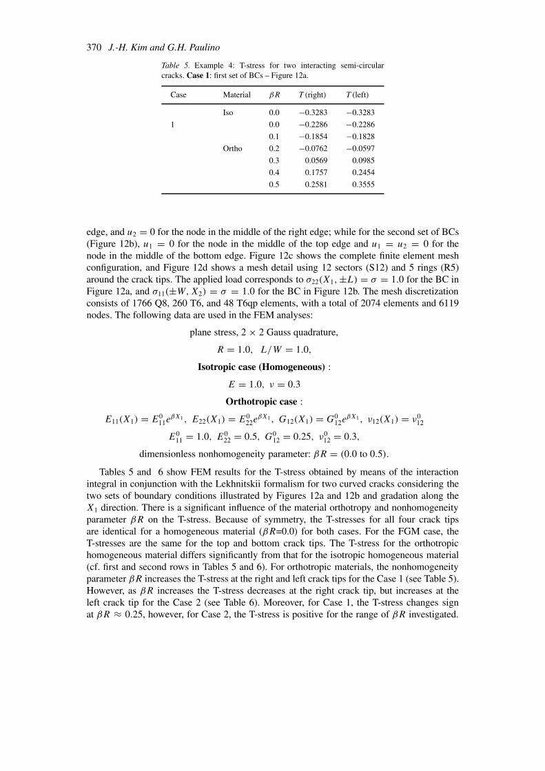
370 J.-H. Kim and G.H. Paulino
Table 5. Example 4: T-stress for two interacting semi-circularcracks. Case 1: first set of BCs – Figure 12a.
Case Material βR T (right) T (left)
Iso 0.0 −0.3283 −0.3283
1 0.0 −0.2286 −0.2286
0.1 −0.1854 −0.1828
Ortho 0.2 −0.0762 −0.0597
0.3 0.0569 0.0985
0.4 0.1757 0.2454
0.5 0.2581 0.3555
edge, and u2 = 0 for the node in the middle of the right edge; while for the second set of BCs(Figure 12b), u1 = 0 for the node in the middle of the top edge and u1 = u2 = 0 for thenode in the middle of the bottom edge. Figure 12c shows the complete finite element meshconfiguration, and Figure 12d shows a mesh detail using 12 sectors (S12) and 5 rings (R5)around the crack tips. The applied load corresponds to σ22(X1,±L) = σ = 1.0 for the BC inFigure 12a, and σ11(±W,X2) = σ = 1.0 for the BC in Figure 12b. The mesh discretizationconsists of 1766 Q8, 260 T6, and 48 T6qp elements, with a total of 2074 elements and 6119nodes. The following data are used in the FEM analyses:
plane stress, 2 × 2 Gauss quadrature,
R = 1.0, L/W = 1.0,
Isotropic case (Homogeneous) :E = 1.0, ν = 0.3
Orthotropic case :E11(X1) = E0
11eβX1, E22(X1) = E0
22eβX1, G12(X1) = G0
12eβX1, ν12(X1) = ν0
12
E011 = 1.0, E0
22 = 0.5, G012 = 0.25, ν0
12 = 0.3,
dimensionless nonhomogeneity parameter: βR = (0.0 to 0.5).
Tables 5 and 6 show FEM results for the T-stress obtained by means of the interactionintegral in conjunction with the Lekhnitskii formalism for two curved cracks considering thetwo sets of boundary conditions illustrated by Figures 12a and 12b and gradation along theX1 direction. There is a significant influence of the material orthotropy and nonhomogeneityparameter βR on the T-stress. Because of symmetry, the T-stresses for all four crack tipsare identical for a homogeneous material (βR=0.0) for both cases. For the FGM case, theT-stresses are the same for the top and bottom crack tips. The T-stress for the orthotropichomogeneous material differs significantly from that for the isotropic homogeneous material(cf. first and second rows in Tables 5 and 6). For orthotropic materials, the nonhomogeneityparameter βR increases the T-stress at the right and left crack tips for the Case 1 (see Table 5).However, as βR increases the T-stress decreases at the right crack tip, but increases at theleft crack tip for the Case 2 (see Table 6). Moreover, for Case 1, the T-stress changes signat βR ≈ 0.25, however, for Case 2, the T-stress is positive for the range of βR investigated.
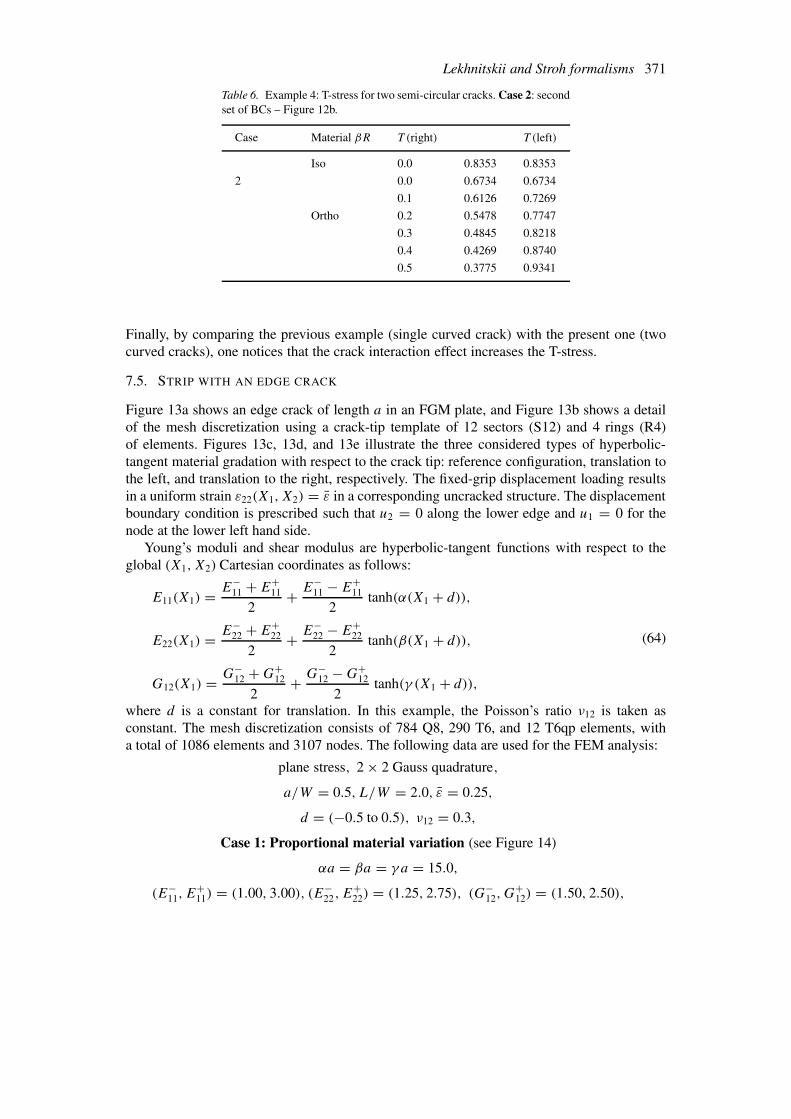
Lekhnitskii and Stroh formalisms 371
Table 6. Example 4: T-stress for two semi-circular cracks. Case 2: secondset of BCs – Figure 12b.
Case Material βR T (right) T (left)
Iso 0.0 0.8353 0.8353
2 0.0 0.6734 0.6734
0.1 0.6126 0.7269
Ortho 0.2 0.5478 0.7747
0.3 0.4845 0.8218
0.4 0.4269 0.8740
0.5 0.3775 0.9341
Finally, by comparing the previous example (single curved crack) with the present one (twocurved cracks), one notices that the crack interaction effect increases the T-stress.
7.5. STRIP WITH AN EDGE CRACK
Figure 13a shows an edge crack of length a in an FGM plate, and Figure 13b shows a detailof the mesh discretization using a crack-tip template of 12 sectors (S12) and 4 rings (R4)of elements. Figures 13c, 13d, and 13e illustrate the three considered types of hyperbolic-tangent material gradation with respect to the crack tip: reference configuration, translation tothe left, and translation to the right, respectively. The fixed-grip displacement loading resultsin a uniform strain ε22(X1, X2) = ε̄ in a corresponding uncracked structure. The displacementboundary condition is prescribed such that u2 = 0 along the lower edge and u1 = 0 for thenode at the lower left hand side.
Young’s moduli and shear modulus are hyperbolic-tangent functions with respect to theglobal (X1, X2) Cartesian coordinates as follows:
E11(X1) = E−11 + E+
11
2+ E−
11 − E+11
2tanh(α(X1 + d)),
E22(X1) = E−22 + E+
22
2+ E−
22 − E+22
2tanh(β(X1 + d)),
G12(X1) = G−12 + G+
12
2+ G−
12 − G+12
2tanh(γ (X1 + d)),
(64)
where d is a constant for translation. In this example, the Poisson’s ratio ν12 is taken asconstant. The mesh discretization consists of 784 Q8, 290 T6, and 12 T6qp elements, witha total of 1086 elements and 3107 nodes. The following data are used for the FEM analysis:
plane stress, 2 × 2 Gauss quadrature,
a/W = 0.5, L/W = 2.0, ε̄ = 0.25,
d = (−0.5 to 0.5), ν12 = 0.3,
Case 1: Proportional material variation (see Figure 14)
αa = βa = γ a = 15.0,
(E−11, E
+11) = (1.00, 3.00), (E−
22, E+22) = (1.25, 2.75), (G−
12,G+12) = (1.50, 2.50),
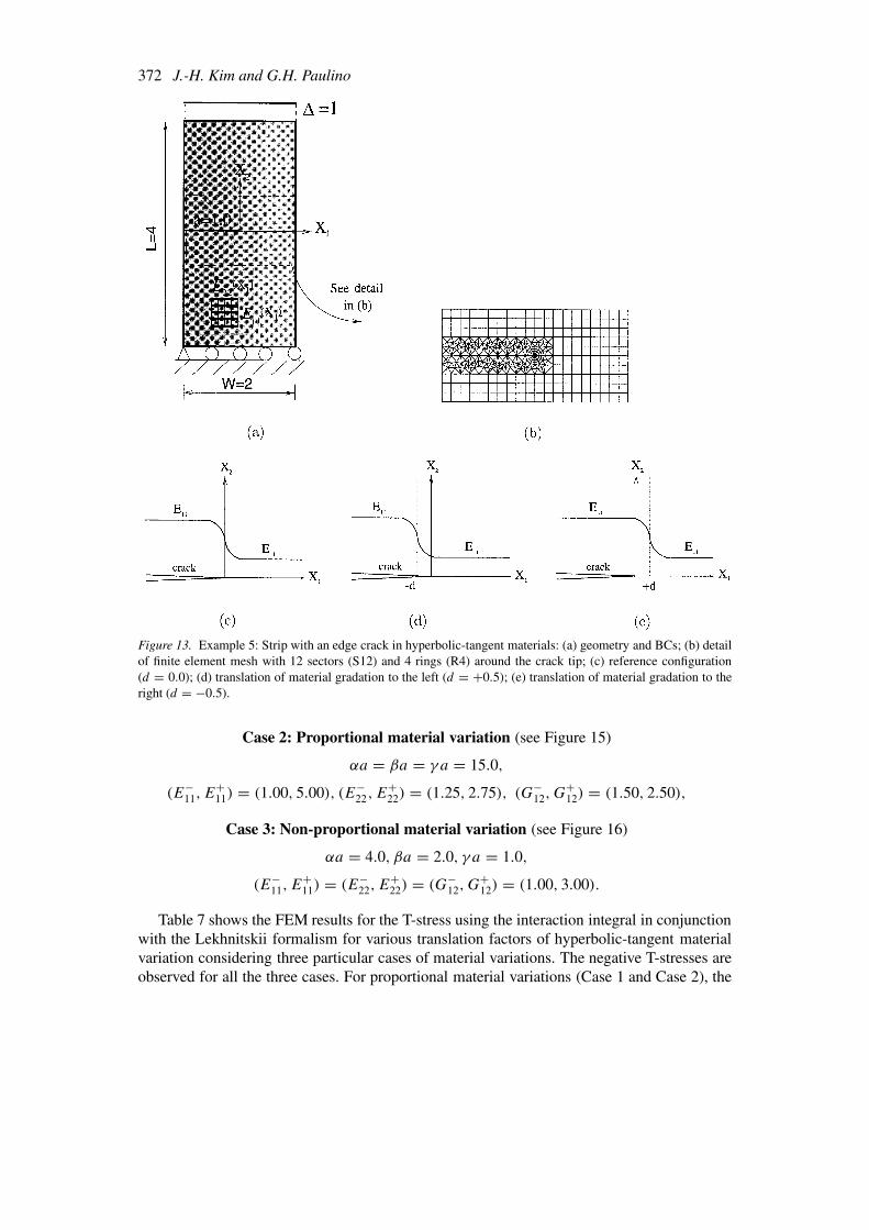
372 J.-H. Kim and G.H. Paulino
Figure 13. Example 5: Strip with an edge crack in hyperbolic-tangent materials: (a) geometry and BCs; (b) detailof finite element mesh with 12 sectors (S12) and 4 rings (R4) around the crack tip; (c) reference configuration(d = 0.0); (d) translation of material gradation to the left (d = +0.5); (e) translation of material gradation to theright (d = −0.5).
Case 2: Proportional material variation (see Figure 15)
αa = βa = γ a = 15.0,
(E−11, E
+11) = (1.00, 5.00), (E−
22, E+22) = (1.25, 2.75), (G−
12,G+12) = (1.50, 2.50),
Case 3: Non-proportional material variation (see Figure 16)
αa = 4.0, βa = 2.0, γ a = 1.0,
(E−11, E
+11) = (E−
22, E+22) = (G−
12,G+12) = (1.00, 3.00).
Table 7 shows the FEM results for the T-stress using the interaction integral in conjunctionwith the Lekhnitskii formalism for various translation factors of hyperbolic-tangent materialvariation considering three particular cases of material variations. The negative T-stresses areobserved for all the three cases. For proportional material variations (Case 1 and Case 2), the

Lekhnitskii and Stroh formalisms 373
Figure 14. Example 5: Proportional variation of material properties (Case 1).
Figure 15. Example 5: Proportional variation of material properties (Case 2).

374 J.-H. Kim and G.H. Paulino
Figure 16. Example 5: Nonproportional variation of material properties (Case 3).
Table 7. Example 5: FEM results for the T-stress for anedge crack with translation of hyperbolic-tangent mater-ial variation. Case 1: proportional material variation (Fig-ure 14); Case 2: proportional material variation (Figure 15);Case 3: Nonproportional material variation (Figure 16).
d T
Case 1 Case 2 Case 3
−0.5 −0.3886 −0.4982 −0.4373
−0.4 −0.4046 −0.5210 −0.4533
−0.3 −0.4310 −0.5715 −0.4754
−0.2 −0.4999 −0.6928 −0.4929
−0.1 −0.7011 −0.9900 −0.4991
0 −0.9667 −1.3870 −0.4714
0.1 −0.3643 −0.4615 −0.4099
0.2 −0.2051 −0.2248 −0.3369
0.3 −0.1706 −0.1773 −0.2749
0.4 −0.1573 −0.1600 −0.2304
0.5 −0.1516 −0.1527 −0.2001

Lekhnitskii and Stroh formalisms 375
Figure 17. Example 6: compact tension (CT) specimen: (a) geometry and BCs; (b) complete finite element mesh.
T-stress decreases with the translation factor d for the range between −0.5 and 0.0, however, itincreases as d increases further. For nonproportional material variations (Case 3), the T-stressdecreases with the translation factor d for the range between −0.5 and −0.1, however, itincreases as d increases further. Moreover, the crack tip location shows a significant influenceon T-stress for all the three cases of hyperbolic-tangent material variation.
7.6. COMPACT TENSION (CT) SPECIMEN
Figure 17a shows the geometry of a CT specimen, and Figure 17b shows the complete finitemesh configuration with 12 sectors (S12) and 4 rings (R4) around the crack tip. The appliedload corresponds to P(0,±0.275) = 1. The displacement boundary condition is prescribed as(u1, u2)(W, 0) = (0, 0) and u2(a, 0) = 0. Young’s moduli and shear modulus are exponentialfunctions of X1, while the Poisson’s ratio is constant. The material properties are given by
For − 0.225W ≤ X1 < 0, E11 = E011, E22 = E0
22,G12 = G012, ν12 = ν0
12,
For 0 ≤ X1 ≤ W, E11 = E011e
βX1, E22 = E022e
βX1,G12 = G012e
βX1 , ν12 = ν012,
(66)
with
E011 = 1, E0
22 = 2,G012 = 0.5, ν0
12 = 0.15. (67)
The following data are used for the FEM analysis:
a/W = 0.1 to 0.8, W = 1
ER = E11(W)/E11(0) = E22(W)/E22(0) = G12(W)/G12(0)
= exp (βW) = (0.1, 0.2, 1.0, 5, 10)
plane stress and 2 × 2 Gauss quadrature.
(68)
Figure 18 shows biaxiality ratio B = T√
πa/KI versus a/W ratio. The mode I SIF KI
is also evaluated by means of the interaction integral method (Kim and Paulino, 2003b). For

376 J.-H. Kim and G.H. Paulino
Figure 18. Example 6: Biaxiality ratio (B = T√
πa/KI ) for a compact tension (CT) specimen. HereER = E11(W)/E11(0) = E22(W)/E22(0) = G12(W)/G12(0) = exp (βW).
both isotropic and orthotropic cases, as the ratio ER = exp(βW) increases, the biaxialityratio increases and the transition points for sign-change of the biaxiality ratio shift to the left.Both material orthotropy and nonhomogeneity show a significant influence on the T-stress andbiaxiality ratio.
8. Concluding remarks and extensions
This paper presents a robust scheme for evaluating the T-stress by means of the interactionintegral (M-integral) method considering arbitrarily oriented straight or curved cracks in two-dimensional (2D) elastic orthotropic nonhomogeneous materials. The scope of the presentformulation is broad enough to cover orthotropic nonhomogeneous, orthotropic homogen-eous, isotropic nonhomogeneous and isotropic homogeneous materials. This paper makesuse of auxiliary fields, which are derived based on two formulations: Lekhnitskii and Stroh.As shown by Barnett and Kirchner (1997), these two formulations are equivalent, and thisequivalence has also been verified in the present work both theoretically and numerically.From numerical investigations, we observe that the T-stress computed by the present methodis reasonably accurate in comparison with available reference solutions, and that materialorthotropy and material nonhomogeneity influences the magnitude and the sign of the T-stress.
Because SIFs and T-stress can be calculated by means of a unified approach using theinteraction integral method, a potential extension of this work includes using these quantitiesas the basis to evaluate crack initiation angle, and develop fracture criteria in orthotropic func-
Lekhnitskii and Stroh formalisms 377
tionally graded materials (see, for example, Boone et al. (1987) for orthotropic homogeneousmaterials using SIF-based techniques).
Acknowledgements
We gratefully acknowledge the support from NASA-Ames, Engineering for Complex SystemsProgram, and the NASA-Ames Chief Engineer (Dr. Tina Panontin) through grant NAG 2-1424. We also acknowledge additional support from the National Science Foundation (NSF)under grant CMS-0115954 (Mechanics & Materials Program). In addition, we would like tothank three anonymous reviewers for their valuable comments and suggestions. Any opin-ions expressed herein are those of the writers and do not necessarily reflect the views of thesponsors.
References
Barnett, D.M. and Kirchner, H.O.K. (1997). A proof of the equivalence of the Stroh and Lekhnitskii sexticequations for plane anisotropic elastostatics. 76(1), 231–239.
Betegón, C. and Hancock, J.W. (1991). Two-parameter characterization of elastic-plastic crack-tip field. Journalof Applied Mechanics, Transactions ASME, 58(1), 104–110.
Boone, T.J. and Wawrzynek, P.A. and Ingraffea, A.R. (1987). Finite element modeling of fracture propagation inorthotropic materials. Engineering Fracture Mechanics, 26(2), 185–201.
Budiansky, B. and Rice, J.R. (1973). Conservation laws and energy-release rates. Journal of Applied Mechanics,Transactions ASME, 40(1), 201–203.
Cardew, G.E., Goldthorpe, M.R., Howard, I.C. and Kfouri, A.P. (1985). On the elastic T-term. Fundamentals ofDeformation and Fracture: Eshelby Memorial Symposium.
Chang, J.H. and Chien, A.J. (2002). Evaluation of M-integral for anisotropic elastic media with multiple defects.International Journal of Fracture, 114(3), 264–289.
Chen, C.S., Krause, R., Pettit, R.G., Banks-Sills, L. and Ingraffea, A.R. (2001). Numerical assessment of T-stresscomputation using a P -version finite element method. International Journal of Fracture 107(2), 177–199.
Cotterell, B. and Rice, J.R. (1980). Sligthly curved or kinked cracks. International Journal of Fracture, 16(2),155–169.
Dolbow, J. and Gosz, M. (2002). On the computation of mixed-mode stress intensity factors in functionally gradedmaterials. International Journal of Solids and Structures, 39(9), 2557–2574.
Du, Z.-Z. and Hancock, J.W. (1991). The effect of non-singular stresses on crack-tip constraint. Journal of theMechanics and Physics of Solids 39(3), 555–567.
Eischen, J.W. (1987). Fracture of non-homogeneous materials. International Journal of Fracture, 34(1), 3–22.Gao, H. and Chiu, C.-H. (1992). Slightly curved or kinked cracks in anisotropic elastic solids. International
Journal of Solids and Structures, 29(8), 947–972.Gu, P., and Asaro, R.J. (1997). Cracks in functionally graded materials. International Journal of Solids and
Structures, 34(1), 1–17.Ilschner, B. (1996). Processing-microstructure-property relationships in graded materials. Journal of the Mechan-
ics and Physics of Solids, 44(5), 647–656.Becker, Jr. T. L., Cannon, R.M. and Ritchie, R.O. (2001). Finite crack kinking in T-stresses in functionally graded
materials. International Journal of Solids and Structures, 38(32–33), 5545-5563.Kanninen, M.F. and Popelar, C.H. (1985). Advanced Fracture Mechanics. Oxford University Press, New York.Kaysser, W.A. and Ilschner, B. (1995). FGM research activities in Europe. M.R.S. Bulletin, 20(1), 22–26.Kfouri, A.P. (1986). Some evaluations of the elastic T-term using Eshelby’s method. International Journal of
Fracture, 30(4), 301–315.Kim, J.-H. (2003). Mixed-mode crack propagation in functionally graded materials. Ph.D. Thesis, University of
Illinois at Urbana-Champaign.Kim, J.-H. and Paulino, G.H. (2002a). Finite element evaluation of mixed-mode stress intensity factors in func-
tionally graded materials. International Journal for Numerical Methods in Engineering, 53(8), 1903–1935.
378 J.-H. Kim and G.H. Paulino
Kim, J.-H. and Paulino, G.H. (2002b). Isoparametric graded finite elements for nonhomogeneous isotropic andorthotropic materials. Journal of Applied Mechanics, Transactions ASME, 69(4), 502–514.
Kim, J.-H. and Paulino, G.H. (2002c). Mixed-mode fracture of orthotropic functionally graded materials usingfinite elements and the modified crack closure method. Engineering Fracture Mechanics, 69(14–16), 1557–1586.
Kim, J.-H. and Paulino, G.H. (2003a). An accurate scheme for mixed-mode fracture analysis of function-ally graded materials using the interaction integral and micromechanics models. International Journal forNumerical Methods in Engineering, 58(10), 1457–1497.
Kim, J.-H. and Paulino, G.H. (2003b). The interaction integral for fracture of orthotropic functionally gradedmaterials: Evaluation of stress intensity factors. International Journal of Solids and Structures, 40(15), 3967–4001.
Kim, J.-H. and Paulino, G.H. (2003c). Mixed-mode J-integral formulation and implementation using graded finiteelements for fracture analysis of nonhomogeneous orthotropic materials. Mechanics of Materials, 35(1–2),107–128.
Kim, J.-H. and Paulino, G.H. (2003d). T-stress, mixed-mode stress intensity factors, and crack initiation angles infunctionally graded materials: A unified approach using the interaction integral method. Computer Methodsin Applied Mechanics and Engineering, 192(11–12), 1463–1494.
Knowles, J.K. and Sternberg, E. (1972). On a class of conservation laws in linearized and finite elastostatics.Archive for Rational Mechanics and Analysis, 44(2), 187–211.
Larsson, S.G. and Carlson, A.J. (1973). Influence of non-singular stress terms and specimen geometry on small-scale yielding at crack tips in elastic-plastic materials. Journal of the Mechanics and Physics of Solids, 21(4),263–277.
Leevers, P.S. and Radon, J.C.D. (1982). Inherent stress biaxiality in various fracture specimen. InternationalJournal of Fracture, 19(4), 311–325.
Lekhnitskii, S.G. (1968). Anisotropic plates. Gordon and Breach Science Publishers, New York.Miyamoto, Y., Kaysser, W.A., Rabin, B.H., Kawasaki, A. and Ford, R.G. (1999). Functionally Graded Materials:
Design, Processing and Applications. Kluwer Academic Publishers, Dordrecht.Muskhelishvili, N.I. (1953). Some Basic Problems of the Mathematical Theory of Elasticity. Noordhoff Ltd.,
Holland.O’Dowd, N.P. and Shih, C.F. (1991). Family of crack-tip fields characterized by a triaxiality parameter - I. structure
of fields. Journal of the Mechanics and Physics of Solids, 39(8), 989–1015.O’Dowd, N.P. and Shih, C.F. (1992). Family of crack-tip fields characterized by a triaxiality parameter - II. fracture
applications. Journal of the Mechanics and Physics of Solids, 40(5), 939–963.O’Dowd, N.P., Shih, C.F. and Dodds Jr., R.H. (1995). The role of geometry and crack growth on constraint and
implications for ductile/brittle fracture. In Constraint Effects in Fracture Theory and Applications, volume 2of ASTM STP 1244, pp. 134–159. American Society for Testing and Materials.
Paulino, G.H., Jin, Z.H. and Dodds Jr., R.H. (2003). Failure of functionally graded materials. In B. Karihalooand W.G. Knauss, editors, Comprehensive Structural Integrity, volume 2, Chapter 13, pp. 607–644. ElsevierScience.
Paulino, G.H. and Kim, J.-H. (2004). A new approach to compute T-stress in functionally graded materials bymeans of the interaction integral method. Engineering Fracture Mechanics, in press.
Raju, I.S. and Shivakumar, K.N. (1990). An equivalent domain integral method in the two-dimensional analysisof mixed mode crack problems. Engineering Fracture Mechanics, 37(4), 707–725.
Rice, J.R. (1968). A path-independent integral and the approximate analysis of strain concentration by notchesand cracks. Journal of Applied Mechanics, Transactions ASME, 35(2), 379–386.
Sampath, S., Herman, H., Shimoda, N. and Saito, T. (1995). Thermal spray processing of FGMs. M.R.S. Bulletin,20(1), 27–31.
Shih, G.C., Paris, P.C. and Irwin, G.R. (1965). On cracks in rectilinearly anisotropic bodies. International Journalof Fracture Mechanics, 1(2), 1989–203.
Sladek, J., Sladek, V. and Fedelinski, P. (1997). Contour integrals for mixed-mode crack analysis: effect ofnonsingular terms. Theoretical and Applied Fracture Mechanics, 27(2), 115–127.
Smith, D.J., Ayatollahi, M.R. and Pavier, M.J. (2001). The role of T-stress in brittle fracture for linear elasticmaterials under mixed-mode loading. Fatigue and Fracture of Engineering Materials and Structures, 24(2),137–150.
Lekhnitskii and Stroh formalisms 379
Suresh, S. and Mortensen, A. (1998). Fundamentals of Functionally Graded Materials. IOM CommunicationsLtd., London.
Ting, C.T.C. (1996). Anisotropic Elasticity: Theory and Applications. Oxford University Press, Oxford.Tokita, M. (1999). Development of large-size ceramic metal bulk FGM fabricated by spark plasma sintering.
Materials Science Forum, 308–311, 83–88.Ueda, Y., Ikeda, K., Yao, T. and Aoki, M. (1983). Characteristics of brittle failure under general combined modes
including those under bi-axial tensile loads. Engineering Fracture Mechanics, 18(6), 1131–1158.Wawrzynek, P.A. (1987). Interactive finite element analysis of fracture process: an integrated approach. M.S.
Thesis, Cornell University.Wawrzynek, P.A. and Ingraffea, A.R. (1991). Discrete modeling of crack propagtion: theorectical aspects and im-
plementation issus in two and three dimensions. Report 91-5, School of Civil Engineering and EnvironmentalEngineering, Cornell University.
Williams, J.G. and Ewing, P.D. (1972). Fracture under complex stress - the angled crack problem. InternationalJournal of Fracture, 8(4), 441–416.
Williams, J.G. (1957). On the stress distribution at the base of a stationary crack. Journal of Applied Mechanics,Transactions ASME, 24(1), 109–114.
Yang, S. and Yuan, F.G. (2000a). Determination and representation of the stress coefficient terms by path-independent integrals in anisotropic cracked solids. International Journal of Fracture, 101(4), 291–319.
Yang, S. and Yuan, F.G. (2000b). Kinked crack in anisotropic bodies. International Journal of Solids andStructures, 37(45), 6635–6682.
Appendix A. derivatives of auxiliary displacements in the Lekhnitskii formalism
The stress-strain relationship, with respect to polar coordinates (r, φ), leads to
εauxrr = ∂ur
∂r= a′
11(φ)A cos φ + B sin φ
rF (φ), (69)
εauxφφ = ur
r+ ∂uφ
r∂φ= a′
12(φ)A cos φ + B sin φ
rF (φ), (70)
εauxrφ = 1
2
(∂ur
r∂φ+ ∂uφ
∂r− uφ
r
)= 0, (71)
where, for the case of material orthotropy directions aligned with the global coordinates,
a′11(φ) = F (φ) = a
tip11 cos4 φ + (2a
tip12 + a
tip66 ) sin2 φ cos2 φ + a
tip22 sin4 φ,
a′12(φ) = a
tip12 + (a
tip11 + a
tip22 − 2a
tip12 − a
tip66 ) sin2 φ cos2 φ.
(72)
Integration of Equation (69) with respect to r leads to
ur = (A cos φ + B sin φ) ln r + g(φ), (73)
where g(φ) is the unknown function of φ. Substitution of Equation (73) into Equation (70)yields
uφ =∫
φ
a′12(φ)
A cos φ+B sin φ
F (φ)dφ−ln r
∫φ
(A cos φ+B sin φ) dφ−∫
φ
g(φ) dφ+h(r), (74)
where the first indefinite integral is not integrable analytically and h(r) is the unknown func-tion of r. By substituting Equations (73) and (74) into Equation (71), one obtains the followingcondition

380 J.-H. Kim and G.H. Paulino
r∂h(r)
∂r− h(r) = 0, (75)
which yields h(r) = Cr with a constant C. Differentiations of ur of Equation (73) and uφ ofEquation (74) with respect to r are
∂ur
∂r= 1
r(A cos φ + B sin φ)
∂uφ
∂r= −1
r(A sin φ − B cos φ) + C,
(76)
where C = 0 because ∂u1/∂r , ∂ur/∂r, and ∂uφ/∂r must have a separable form of (1/r) ×p(φ). Then
∂u1
∂r= ∂ur
∂rcos φ − ∂uφ
∂rsin φ = A
r. (77)
Using the chain rule of differentiation and Equation (77), one writes
u1,1 = ∂u1
∂r
∂r
∂X1+ ∂u1
∂φ
∂φ
∂X1= (a
tip11 cos2 φ + a
tip12 sin2 φ)
A cos φ + B sin φ
rF (φ), (78)
with
∂r
∂X1= cos φ,
∂r
∂X2= sin φ,
∂φ
∂X1= − sin φ
r,
∂φ
∂X2= cos φ
r.
(79)
By means of the same procedure above, one obtains u2,2 as
u2,2 = ∂u2
∂r
∂r
∂X2+ ∂u2
∂φ
∂φ
∂X2= (a
tip12 cos2 φ + a
tip22 sin2 φ)
A cos φ + B sin φ
rF (φ). (80)
Solution of Equation (78) for the unknown ∂u1/∂φ leads to
∂u1
∂φ= − 1
F (φ)(AH1(φ) + BH2(φ)), (81)
where H1(φ) and H2(φ) are given by Equation (15). Using ∂u1/∂r (Equation (77)) and∂u1/∂φ (Equation (81)), one obtains u1,2 and u2,1 as follows:
u1,2 = ∂u1
∂r
∂r
∂X2+ ∂u1
∂φ
∂φ
∂X2
u2,1 = 2atip66 σ aux
12 − u1,2.
(82)
The expressions for derivatives of displacements ui,j (i, j = 1, 2) are given in Equation (14).
Appendix B. Stroh Formalism
Let’s consider an orthotropic linear elastic body in two dimensional fields. According to theStroh formalism, the displacement vector u and the stress function vector � are given by(Ting, 1996)

Lekhnitskii and Stroh formalisms 381
u = Re [A f (z) d], � = Re [B f (z) d], (83)
where
σi1 = −�i,2, σi2 = �i,1
A = [a1, a2], B = [b1, b2],f (z) = diag[f (z1), f (z2)], zk = x1 + µkx2, Im[µk] > 0 (k = 1, 2),
(84)
in which f (z) is a diagonal matrix of an arbitrary complex function; d is an unknown complexconstant vector; µk, ak and bk are the Stroh eigenvalues and eigenvectors, respectively, whichare functions of material parameters. These are obtained by the following eigenvalue problem(Ting, 1996):
Np = µp, (85)
where
N =[
N1 N2
N3 NT1
],p =
[a
b
],
N1 = −T −1RT , N2 = T −1, N3 = RT −1RT − Q,
(86)
in which Q, R and T are 2×2 matrices given by:
Qij = Ci1j1, Rij = Ci1j2, Tij = Ci2j2 with σpq = Cpqstεst . (87)
Since the 4×4 matrix N is not symmetric and the strain energy is positive definite, there existtwo pairs of complex conjugates for µ as follows:
µk = µk, ak+2 = ak, bk+2 = bk, (k = 1, 2). (88)
Because N is not symmetric, the p in Equation (85) is a right eigenvector. The right eigen-vector q satisfies the following eigen-relation (Ting, 1996):
NT q = µq (89)
and is given by
q =[
b
a
]. (90)
For different eigenvalues (µk �= µl) the left and right eigenvectors are orthogonal to eachother, i.e.
qkpl = 0. (91)
Assuming that µk are distinct, we normalize pk such that
qkpl = δkl or bTk al + aT
k bl = δkl, (92)
where δkl is the Kronecker delta. Combining Equations (91) with (92) leads to[BT AT
BT
AT
][A A
B B
]=[
I 0
0 I
], (93)
382 J.-H. Kim and G.H. Paulino
where I is the 2 × 2 identity matrix. The 4 × 4 matrices on the left of Equation (93) are theinverses to each other. Thus[
A A
B B
][BT AT
BT
AT
]=[
I 0
0 I
], (94)
or
ABT + A BT = I = BAT + B A
T
AAT + A AT = 0 = BBT + B B
T.
(95)
Equation (95) shows that the real part of ABT is I /2, and AAT and BBT are purely imaginary.Thus the three real matrices are defined as follows (Ting, 1996):
S = i(2ABT − I ), H = 2iAAT , L = −2iBBT . (96)

Lekhnitskii and Stroh formalisms 383
Appendix C. Nomenclature
a half crack length
aij contracted notation of the compliance tensor for plane stress; i = 1,2,6; j = 1,2,6
atipij aij evaluated at the crack tip location; i, j = 1,2,6
A a 2 × 2 complex matrix
bij contracted notation of the compliance tensor for plane strain; i = 1,2,6; j = 1, 2, 6
btipij bij evaluated at the crack tip location; i, j = 1, 2, 6
B a 2 × 2 complex matrix
Cijkl constitutive tensor for anisotropic materials; i, j, k, l = 1, 2, 3
d translation factor in hyperbolic-tangent function
e natural logarithm base, e = 2.71828182 . . .
E11, E22 Young’s moduli with respect to the principal axes of orthotropy
E011, E0
22 Young’s moduli E11, E22 evaluated at the origin
f a point force
f an arbitrary complex function
G12 shear modulus in orthotropic materials
G012 shear modulus G12 evaluated at the origin
h1, h2 dimensions of the beam specimen
H length of material gradation
I the 2 × 2 identity matrix
H a 2 × 2 real matrix
H contour integral
Im imaginary part of the complex function
J path-independent J -integral for the actual field
Jaux J -integral for the auxiliary field
J s J -integral for the superimposed fields (actual plus auxiliary)
KI mode I stress intensity factor
KII mode II stress intensity factor
L length of a plate
L a 2 × 2 real matrix
M interaction integral (M-integral)
N a 4 × 4 complex matrix
N3 a 2 × 2 complex matrix
mi , ni unit normal vectors on the contour of the domain integral

384 J.-H. Kim and G.H. Paulino
Nomenclature (Continued)
pk coefficients of the asymptotic displacements for orthotropic materials; k = 1, 2
qk coefficients of the asymptotic displacements for orthotropic materials; k = 1, 2
q weight function in the domain integral
Q a 2 × 2 real matrix
r radial direction in polar coordinates
R a 2 × 2 real matrix
Re real part of the complex function
S a 2 × 2 real matrix
T a 2 × 2 real matrix
T T-stress
ui displacements for the actual field; i = 1, 2
uauxi
displacements for the auxiliary field; i = 1, 2
u 2 × 2 displacement vector
uaux 2 × 2 auxiliary displacement vector
W width of a plate
W strain energy density
Waux strain energy density for the auxiliary field
xi local Cartesian coordinates; i = 1, 2
Xi global Cartesian coordinates; i = 1, 2
zk complex variable, zk = xk + iyk ; k = 1, 2
α material nonhomogeneity parameter for gradation of E11
αk the real part of µk ; k = 1, 2
β material nonhomogeneity parameter for gradation of E22
βk the imaginary part of µk ; k = 1, 2
γ material nonhomogeneity parameter for gradation of G12
� contour for J and M integrals
�0 outer contour
�s inner contour
�+ contour along the upper crack face
�− contour along the lower crack face
δij Kronecker delta; i, j = 1, 2
εk contracted notation of εij ; k = 1, . . . , 6
εij strains for the actual fields; i = 1, 2, 3; j = 1, 2, 3
µk roots of the characteristic equation; k = 1, 2
µtipk
µk evaluated at the crack tip location; k = 1, 2
µk complex conjugate of µk ; k = 1, 2
νij Poisson’s ratio representing the response in direction j due to loading in direction i
σk contracted notation of σij ; k = 1, . . . , 6
σij stresses for the actual fields; i=1,2,3; j = 1, 2, 3
σauxij stresses for the auxiliary fields; i = 1, 2, 3; j = 1, 2, 3
φ angular direction in polar coordinates with respect to the global Cartesian coordinates
� stress function vector
ω angular direction in polar coordinates with respect to the local Cartesian coordinates