t racking l earning d etection - surrey · racking earning etection zdenek kalal submitted for the...
TRANSCRIPT

T
L
D
RACKING
EARNING
ETECTION
Zdenek Kalal
Submitted for the degree ofDoctor of Philosophy
Centre for Vision, Speech and Signal ProcessingFaculty of Engineering and Physical Sciences
University of Surrey
April 2011
c© Zdenek Kalal 2011


Summary
Visual tracking is the process of locating an object in a video sequence. This thesisinvestigates visual tracking of an unknown object, which significantly changes its ap-pearance and moves in and out of the camera view. The object is defined by its locationand extent in a single frame. In every frame that follows, the task is to determine theobject’s location and extent or indicate that the object is not present.
We propose a novel tracking paradigm (TLD) that decomposes the visual tracking taskinto three sub-tasks: Tracking, Learning and Detection. The tracker follows the objectfrom frame to frame. The detector localizes appearances that have been observedduring tracking and corrects the tracker if necessary. Exploiting the spatio-temporalstructure in the video sequence, the learning component estimates errors performedby the detector and updates it to avoid these errors in the future. The components areanalyzed in detail.
In tracking, we develop a method for detection of tracking failures that we call Forward-Backward (FB) error. The FB error allows us to measure the reliability of point trajec-tories in video. Next, we design a novel object tracker, which represents the object ofinterest by a grid of points the reliability of which is measured using the FB error. Theperformance of the tracker is compared with state-of-the-art approaches.
In detection, we focus on supervised learning of object detectors from large data sets.We develop a learning algorithm that optimally combines two popular learning ap-proaches: boosting and bootstrapping. The improvements in terms of classifier speedand accuracy are achieved.
In learning, we focus on incremental, real-time learning of object detectors from avideo stream. We develop a novel learning theory, P-N learning, which drives thelearning process by a pair of ”experts” on estimation of detector errors: (i) P-expertestimates missed detections; (ii) N-expert estimates false alarms. Convergence prop-erties of the learning method are analyzed and conditions that guarantee improvementof the detector are found. The theory is validated on both synthetic and real data andspecific examples of the experts are given.
Finally, a real-time implementation of the TLD is described and comparatively evalu-ated on benchmark sequences. A significant improvement over state-of-the-art meth-ods is achieved.
Key words: tracking, learning, detection, unsupervised bootstrapping

Email: [email protected]

Acknowledgements
I would like to thank my suppervisors Dr. Krystian Mikolajczyk and Prof. Jiri Matas.This thesis would not have been possible without their valuable feedback.
I am grateful to my colleagues: Asish Gupta, Martin Klaudiny and Stuart James forproofreading parts of this thesis and the whole CVSSP for a nice working atmosphere.
Most importantly, I want to thank to my family for endless support throughout mywhole studies. My final and very special thanks goes to Sayaka, for her support, com-prehension and encouragement.

vi

Contents
1 Introduction 15
1.1 Objectives . . . . . . . . . . . . . . . . . . . . . . . . . . . . . . . . 15
1.2 Motivation . . . . . . . . . . . . . . . . . . . . . . . . . . . . . . . . 16
1.3 Challenges . . . . . . . . . . . . . . . . . . . . . . . . . . . . . . . . 19
1.4 Contributions . . . . . . . . . . . . . . . . . . . . . . . . . . . . . . 22
1.5 Thesis outline . . . . . . . . . . . . . . . . . . . . . . . . . . . . . . 24
1.6 Publications . . . . . . . . . . . . . . . . . . . . . . . . . . . . . . . 26
2 Related work 27
2.1 Tracking . . . . . . . . . . . . . . . . . . . . . . . . . . . . . . . . . 28
2.1.1 Prerequisites . . . . . . . . . . . . . . . . . . . . . . . . . . 28
2.1.2 Classification . . . . . . . . . . . . . . . . . . . . . . . . . . 30
2.1.3 Generative trackers . . . . . . . . . . . . . . . . . . . . . . . 31
2.1.4 Discriminative trackers . . . . . . . . . . . . . . . . . . . . . 35
2.2 Detection . . . . . . . . . . . . . . . . . . . . . . . . . . . . . . . . 39
2.2.1 Detection of image features . . . . . . . . . . . . . . . . . . 40
2.2.2 Detection of object instances . . . . . . . . . . . . . . . . . . 40
2.2.3 Detection of faces . . . . . . . . . . . . . . . . . . . . . . . 43
2.3 Machine learning . . . . . . . . . . . . . . . . . . . . . . . . . . . . 46
2.3.1 Bootstrapping . . . . . . . . . . . . . . . . . . . . . . . . . . 47
2.3.2 Boosting . . . . . . . . . . . . . . . . . . . . . . . . . . . . 49
2.3.3 Semi-supervised learning . . . . . . . . . . . . . . . . . . . . 52
2.4 Observations . . . . . . . . . . . . . . . . . . . . . . . . . . . . . . 55
vii

viii Contents
3 Tracking: failure detection 57
3.1 Detection of tracking failures . . . . . . . . . . . . . . . . . . . . . . 57
3.1.1 Forward-Backward error . . . . . . . . . . . . . . . . . . . . 59
3.1.2 Quantitative evaluation . . . . . . . . . . . . . . . . . . . . . 60
3.1.3 Visualization . . . . . . . . . . . . . . . . . . . . . . . . . . 62
3.2 Median-Flow tracker . . . . . . . . . . . . . . . . . . . . . . . . . . 64
3.2.1 Quantitative evaluation . . . . . . . . . . . . . . . . . . . . . 66
3.3 Conclusions . . . . . . . . . . . . . . . . . . . . . . . . . . . . . . . 68
4 Detection: supervised bootstrap 71
4.1 Introduction . . . . . . . . . . . . . . . . . . . . . . . . . . . . . . . 72
4.2 Related work . . . . . . . . . . . . . . . . . . . . . . . . . . . . . . 73
4.3 Integration of bootstrapping and boosting . . . . . . . . . . . . . . . 73
4.3.1 Known sampling strategies . . . . . . . . . . . . . . . . . . . 76
4.3.2 Proposed sampling strategies . . . . . . . . . . . . . . . . . . 77
4.3.3 Properties of sampling strategies . . . . . . . . . . . . . . . . 80
4.4 Application to face detection . . . . . . . . . . . . . . . . . . . . . . 83
4.4.1 Frontal face detector . . . . . . . . . . . . . . . . . . . . . . 84
4.4.2 Profile face detector . . . . . . . . . . . . . . . . . . . . . . 85
4.4.3 Specific face detector . . . . . . . . . . . . . . . . . . . . . . 86
4.5 Conclusions . . . . . . . . . . . . . . . . . . . . . . . . . . . . . . . 86
5 Learning: unsupervised bootstrap 89
5.1 Introduction . . . . . . . . . . . . . . . . . . . . . . . . . . . . . . . 89
5.2 P-N learning . . . . . . . . . . . . . . . . . . . . . . . . . . . . . . . 91
5.2.1 Formalization . . . . . . . . . . . . . . . . . . . . . . . . . . 91
5.2.2 Stability . . . . . . . . . . . . . . . . . . . . . . . . . . . . . 94
5.2.3 Experiments . . . . . . . . . . . . . . . . . . . . . . . . . . 97
5.3 Learning an object detector from a video sequence . . . . . . . . . . 99

Contents ix
5.3.1 Problem specification . . . . . . . . . . . . . . . . . . . . . . 100
5.3.2 P-N experts . . . . . . . . . . . . . . . . . . . . . . . . . . . 101
5.3.3 Experiments . . . . . . . . . . . . . . . . . . . . . . . . . . 105
5.4 Conclusions . . . . . . . . . . . . . . . . . . . . . . . . . . . . . . . 109
6 Tracking-Learning-Detection (TLD) 111
6.1 Introduction . . . . . . . . . . . . . . . . . . . . . . . . . . . . . . . 111
6.2 Framework . . . . . . . . . . . . . . . . . . . . . . . . . . . . . . . 113
6.2.1 Components . . . . . . . . . . . . . . . . . . . . . . . . . . 113
6.2.2 Initialization . . . . . . . . . . . . . . . . . . . . . . . . . . 114
6.2.3 Run-time . . . . . . . . . . . . . . . . . . . . . . . . . . . . 115
6.3 Implementation . . . . . . . . . . . . . . . . . . . . . . . . . . . . . 115
6.3.1 Object representation . . . . . . . . . . . . . . . . . . . . . . 116
6.3.2 The object model . . . . . . . . . . . . . . . . . . . . . . . . 116
6.3.3 The object detector . . . . . . . . . . . . . . . . . . . . . . . 118
6.3.4 The object tracker . . . . . . . . . . . . . . . . . . . . . . . 122
6.3.5 The integrator . . . . . . . . . . . . . . . . . . . . . . . . . . 122
6.3.6 The learning component . . . . . . . . . . . . . . . . . . . . 123
6.4 Quantitative evaluation . . . . . . . . . . . . . . . . . . . . . . . . . 126
6.4.1 Comparison 1: CoGD . . . . . . . . . . . . . . . . . . . . . 127
6.4.2 Comparison 2: PROST . . . . . . . . . . . . . . . . . . . . . 127
6.4.3 Comparison 3: TLD data set . . . . . . . . . . . . . . . . . . 128
6.5 Long-term tracking of faces . . . . . . . . . . . . . . . . . . . . . . . 132
6.5.1 Sitcom episode . . . . . . . . . . . . . . . . . . . . . . . . . 132
6.5.2 Surveillance footage . . . . . . . . . . . . . . . . . . . . . . 133
6.6 Qualitative analysis . . . . . . . . . . . . . . . . . . . . . . . . . . . 135
6.6.1 Strengths . . . . . . . . . . . . . . . . . . . . . . . . . . . . 135
6.6.2 Weaknesses . . . . . . . . . . . . . . . . . . . . . . . . . . . 138

x Contents
7 Discussion 141
7.1 Contributions . . . . . . . . . . . . . . . . . . . . . . . . . . . . . . 141
7.2 Recent development . . . . . . . . . . . . . . . . . . . . . . . . . . . 143
7.3 Future work . . . . . . . . . . . . . . . . . . . . . . . . . . . . . . . 144
A Compared algorithms 147
B Sequences used for evaluation 149
Bibliography 153

List of Figures
1.1 The long-term tracking task and the achieved results. The top row
depicts the objects of interest selected for tracking. The remaining
images show the results of our long-term tracker. The red dots indicate
that the object is not visible. . . . . . . . . . . . . . . . . . . . . . . 17
1.2 Challenges in long-term tracking: occlusion and disappearance. . . . 20
1.3 Challenges in long-term tracking: appearance and viewpoint changes. 20
1.4 Challenges in long-term tracking: background clutter and identification. 21
1.5 Challenges in long-term tracking: scale changes. . . . . . . . . . . . 21
1.6 Challenges in long-term tracking: illumination changes. All images
have been equalized. . . . . . . . . . . . . . . . . . . . . . . . . . . 22
1.7 Challenges in long-term tracking: motion blur. . . . . . . . . . . . . 22
1.8 The block diagram of the proposed TLD framework. . . . . . . . . . 23
1.9 Outline and main contributions of the thesis. . . . . . . . . . . . . . . 25
2.1 Illustration of a typical tracking system. . . . . . . . . . . . . . . . . 28
2.2 Classification of trackers based the representation of the object: a)
points, b) geometric shapes, c) contours, d) articulated models, and
e) motion field. . . . . . . . . . . . . . . . . . . . . . . . . . . . . . 29
1

2 List of Figures
2.3 The WSL tracker [Jepson 03] estimates components on a template that
are reliable for tracking. This increases the tracker’s robustness to par-
tial occlusion and appearance changes. . . . . . . . . . . . . . . . . 33
2.4 Incremental Visual Tracking [Ross 07] builds online a PCA-based model
of the object. The method demonstrated a strong resistance to appear-
ance and illumination variations. . . . . . . . . . . . . . . . . . . . . 34
2.5 Ensemble tracking [Avidan 07] represents the object of interest by a
discriminative model classifying every pixel as the object or back-
ground. The classifier is adapted in every frame. The tracker demon-
strated the ability to handle appearance changes in presence of clut-
tered environment. . . . . . . . . . . . . . . . . . . . . . . . . . . . 36
2.6 The SemiBoost tracker [Grabner 08] reduces drift of discriminative
trackers by guiding the update by an offline trained classifier. Per-
formance was demonstrated (among others) on: (TOP) 24h tracking of
a still object by static camera, (BOTTOM) re-detection of a stationary
object after a brief occlusion. . . . . . . . . . . . . . . . . . . . . . . 36
2.7 Illustration of a typical detection system. . . . . . . . . . . . . . . . 39
2.8 Lowe [Lowe 04] proposed a detection system that represented objects
locally using keypoints and SIFT descriptors. The detector is based
on an approximate nearest neighbor and global geometric constraints.
The system demonstrated a significant illumination and pose invari-
ance and robustness to partial occlusions. . . . . . . . . . . . . . . . 41
2.9 Feature harvesting [Ozuysal 06], a method for automatic training of an
object detector in a controlled environment (TOP). After the training
phase the detector operates in cluttered environments (BOTTOM). . . . 42
2.10 Illustration of a typical face detection components. . . . . . . . . . . 43

List of Figures 3
2.11 Features used to represent appearance in objects detection. . . . . . . 45
2.12 Classification of learning methods. Colored dots correspond to labeled
training examples; white dots correspond to unlabeled examples. . . . 46
2.13 Bootstrapping: a) the block diagram, b) an initial training set, c) a
training set after several iterations of bootstrapping. . . . . . . . . . . 47
2.14 Boosting: a) the block diagram, b) a weak classifier and a weighted
training set, c) a strong classifier. . . . . . . . . . . . . . . . . . . . . 48
2.15 Standard AdaBoost versus cascaded AdaBoost: (TOP) standard Ad-
aBoost has to evaluate all weak classifiers (here Haar-like filters), (BOT-
TOM) cascaded AdaBoost enables to reject negative examples after
each stage of the classifier thus reducing the computation demands. . . 51
2.16 Can unlabeled data improve a classifier? Refer to the text for explanation. 52
2.17 Illustration of co-training [Blum 98] of two classifiers. . . . . . . . . 54
3.1 Illustration of the Forward-Backward error measure: (TOP) consis-
tent (1) and inconsistent (2) trajectories, (BOTTOM) terms used for the
definition of the Forward-Backward error measure. . . . . . . . . . . 59
3.2 Quantitative evaluation of the Forward-Backward error for k = 1.
(TOP) Precision and recall as a function of threshold θ. (BOTTOM)
Precision and recall characteristics in comparison to Sum of Square
Differences. . . . . . . . . . . . . . . . . . . . . . . . . . . . . . . . 61
3.3 Error map: visualization of the Forward-Backward error for k = 50.
Dark colors in the error map indicate low Forward-Backward error that
considers 50 frames. Yellow points in the original frames indicate 5%
of the most reliable points. Points on the pedestrians are enlarged for
better visibility. . . . . . . . . . . . . . . . . . . . . . . . . . . . . . 63

4 List of Figures
3.4 The block diagram of the Median-Flow tracker. . . . . . . . . . . . . 64
3.5 Estimation of the object motion using median. Only translation is il-
lustrated, Median-Flow estimates scale as well. . . . . . . . . . . . . 65
3.6 Comparison of various variants of the Median-Flow tracker. . . . . . 67
3.7 Several frames from the sequence CAR overlaid with the output of
the Median-Flow tracker (yellow) and 50% of the most reliable points
(blue). Notice that the points are covering the visible parts of the
tracked object. The points that cover occluded or low-textured parts
of the object are automatically filtered out by the Forward-Backward
error. . . . . . . . . . . . . . . . . . . . . . . . . . . . . . . . . . . 68
4.1 Illustration of standard boosting (LEFT) and boosting combined with
bootstrapping (RIGHT). . . . . . . . . . . . . . . . . . . . . . . . . . 74
4.2 Illustration of bias and variance of a bootstrapping strategy. . . . . . 76
4.3 Pool with weights di (blue bars) is repeatedly sampled to obtain a dis-
tribution of the estimated weights. The range of the distribution (1 and
99% quantiles) is depicted by red vertical lines and expected values by
circles. . . . . . . . . . . . . . . . . . . . . . . . . . . . . . . . . . . 81
4.4 The variance and bias of the sampling strategies. The dashed line
shows the exponential loss of the optimal hypothesis. (a) Exponen-
tial loss measured of a given hypotheis, (b) exponential loss measured
on training data, (c) exponential loss measured on testing data. See
text for more details. . . . . . . . . . . . . . . . . . . . . . . . . . . 82
4.5 The detector performance as a function of the active set size and the
sampling strategy. The pool consists of 10 000 positive and 56 million
negative examples. . . . . . . . . . . . . . . . . . . . . . . . . . . . 84

List of Figures 5
4.6 Performance evaluation: (LEFT) ROC curves on CMU-MIT profile
database (368 profile faces in 208 images). (RIGHT) PRC for specific
face detector applied on the results of Google face search. . . . . . . . 85
4.7 Results achieved by our face detector. Bottom row shows the most
challenging faces. The binary executable is available at the website of
the author. . . . . . . . . . . . . . . . . . . . . . . . . . . . . . . . . 87
5.1 The block diagram of the P-N learning. . . . . . . . . . . . . . . . . 91
5.2 The evolution of errors of the classifier depends on the quality of the P-
N experts, which is defined in terms of eigenvalues of matrix M. The
errors converge to zero (LEFT), are at the edge of stability (MIDDLE)
or are growing (RIGHT). . . . . . . . . . . . . . . . . . . . . . . . . 96
5.3 Performance of a detector as a function of the number of processed
frames. The detectors were trained by synthetic P-N experts with
guaranteed level of error. The classifier is improved up to error 50%
(BLACK), higher error degrades it (RED). . . . . . . . . . . . . . . . 98
5.4 Performance of detectors trained by error-less P-expert, N-expert and
P-N expert measured by precision (LEFT), recall (MIDDLE) and f-
measure (RIGHT). . . . . . . . . . . . . . . . . . . . . . . . . . . . 99
5.5 Given a single example and a video stream, the goal of P-N learning is
to train an accurate object detector. . . . . . . . . . . . . . . . . . . . 100
5.6 Illustration of P-N experts: (a) output of an motorbike detector, (b)
errors identified by P-N experts. . . . . . . . . . . . . . . . . . . . . 101
5.7 Illustration of a scanning grid applied to three consecutive frames (a)
and corresponding spatio-temporal volume of labels with unacceptable
(b) and acceptable (c) labeling. Red dots correspond to positive labels. 103
5.8 Illustration of the P-expert and the N-expert and their error compensation.104
6 List of Figures
5.9 Sample images from evaluation sequences with objects marked. See
Appendix B for more details. . . . . . . . . . . . . . . . . . . . . . . 106
5.10 Several snapshot from face sequence that has been used to evaluate
repeated runs of P-N learning. . . . . . . . . . . . . . . . . . . . . . 107
6.1 Illustration of a tracker (a), detector (b), and a tractor (c). Dotted line
shows ground truth trajectory, gray bar represents full occlusion, thick
line is the trajectory of a tracker, red dots are responses of a detector. . 112
6.2 Detailed block diagram of the TLD framework. . . . . . . . . . . . . 113
6.3 Illustration of a trajectory in video volume and corresponding trajec-
tory in the appearance space. . . . . . . . . . . . . . . . . . . . . . . 117
6.4 The block diagram of the object detector. . . . . . . . . . . . . . . . 119
6.5 The block diagram of our ensemble classifier. . . . . . . . . . . . . . 120
6.6 Conversion of a patch to a binary code using a set of pixel comparisons. 120
6.7 Pixel comparisons measured within individual base classifiers. The
rectangles correspond to a normalized patch. Squares correspond to
pixel locations, lines show which pixels are compared. . . . . . . . . 120
6.8 Illustration of integrator: (a) the object is tracked and detected, (b) the
tracker is challenged by occlusion, detector has no response, (c) the
tracker failed, the detector re-detects the object; these two patches are
assigned conservative similarity Sc. Appearance that is in the online
model earlier (car) receives higher score, new appearance (failed) re-
ceives lower score and the tracker is re-initialized (arrow). . . . . . . 123
6.9 Illustration of the P-expert: (a) an object model in a feature space and
the core (gray blob); (b) a non-reliable trajectory (dotted line) and a
reliable trajectory (thick line); (c) the object model and the core after
the update. . . . . . . . . . . . . . . . . . . . . . . . . . . . . . . . 126

List of Figures 7
6.10 Evaluation of Face-TLD on a sitcom episode “IT crowd”. (TOP-LEFT)
The initial frame. The entire sequence (22 minutes) was then processed
automatically. . . . . . . . . . . . . . . . . . . . . . . . . . . . . . . 134
6.11 Evaluation of Face-TLD on sequence Surveillance. (LEFT) Responses
of generic face detector (red), detections approved by online learned
model (black), ground truth trajectory of the subject (blue). (RIGHT)
The surveillance scenario. . . . . . . . . . . . . . . . . . . . . . . . 134
6.12 TLD1.0 and scale changes. . . . . . . . . . . . . . . . . . . . . . . . 136
6.13 TLD1.0 and illumination changes. . . . . . . . . . . . . . . . . . . . 136
6.14 TLD1.0 and appearance changes. . . . . . . . . . . . . . . . . . . . . 137
6.15 TLD1.0 and partial occlusions. . . . . . . . . . . . . . . . . . . . . . 137
6.16 TLD1.0 and re-detection. . . . . . . . . . . . . . . . . . . . . . . . . 138
6.17 TLD1.0 and similar targets. The sequence appeared in [Kwon 10]. . . 138
6.18 Out-of-plane rotations are challenging for TLD1.0. The sequence ap-
peared in [Leichter 09]. . . . . . . . . . . . . . . . . . . . . . . . . . 139
6.19 TLD1.0 and sequences where the object never re-appear in a similar
view. The sequence appeared in [Kwon 10]. . . . . . . . . . . . . . . 139
7.1 TLD demo at Computer Vision and Pattern Recognition conference,
2010. . . . . . . . . . . . . . . . . . . . . . . . . . . . . . . . . . . 144
B.1 Snapshots from the sequences used for evaluation. A horizontal line
separates the standard and the introduced sequences. . . . . . . . . . 151

8 List of Figures

List of Tables
3.1 Comparison of the Median-Flow tracker with state-of-the-art approaches
in terms of the number of correctly tracked frames. . . . . . . . . . . 67
4.1 Data sets used for training of a face detector. . . . . . . . . . . . . . . 83
5.1 Performance analysis of P-N learning. The Initial detector is trained
on the first frame only. The Final detector is obtained by P-N learning
after one pass through the sequence. The P-N Tracker is the adap-
tive Lucas-Kanade tracker re-initialized by the on-line trained detec-
tor. The last three columns display internal statistics of the training
process. The statistics were computed for every frame and the table
reports the average values. . . . . . . . . . . . . . . . . . . . . . . . 107
5.2 Performance of P-N learning as a number of runs through the video. . 108
6.1 The number of successfully tracked frames – TLD1.0 in comparison
to results reported in [Yu 08]. Bold numbers indicate the best score; a
dash indicates that the result was not reported. TLD1.0 achieved the
best possible performance. . . . . . . . . . . . . . . . . . . . . . . . 128
6.2 Recall – TLD1.0 in comparison to results reported in [Santner 10].
Bold numbers indicate the best score; a dash indicates that the result
was not reported. TLD1.0 scored best in 9/10 sequences. . . . . . . . 129
9

10 List of Tables
6.3 Localization error (pixels) – TLD1.0 in comparison to results reported
in [Santner 10]. Bold numbers indicate the best score; a dash indicates
that the result was not reported. TLD1.0 scored best in 7/10 sequences. 129
6.4 F-measure – performance on the TLD data set. Bold numbers indicate
the best score. TLD1.0 scored best in 9/10 sequences. . . . . . . . . 131
6.5 Precision – performance on the TLD data set. Bold numbers indicate
the best score. TLD1.0 achieved the precision of 82%, the second best
achieved 80%. . . . . . . . . . . . . . . . . . . . . . . . . . . . . . . 132
6.6 Recall – performance on the TLD data set. Bold numbers indicate the
best score. TLD1.0 achieved recall of 81%, the second best achieved
18%. . . . . . . . . . . . . . . . . . . . . . . . . . . . . . . . . . . . 133
B.1 Description of sequences used for evaluation. A horizontal line sep-
arates the standard and the introduced sequences. The red color indi-
cates sequences from the TLD data set. . . . . . . . . . . . . . . . . . 150

List of Tables 11

12 List of Tables
Notation and Symbols
I image
p image point
b bounding box
P image patch extracted around p or within b
x sample, a representation of P in a feature space X
d sample weight
d approximated sample weight
y sample label from space of labels Y = {-1,1}
X set of samples x
Y set of labels y
L labeled set, a set of pairs (x, y)
D set of weights d
M object model, a set of patches P
D approximated set of weights d−→T k trajectory of an image point tracked for k frames forward in time←−T k trajectory of an image point tracked for k frames backward in time
f(x|Θ) classifier that realizes mapping X → Y
h(x) weak hypothesis that realizes mapping X → R
H(x) strong hypothesis that realizes mapping X → R
S similarity function
Sr relative similarity function
Sc conservative similarity function
θNN threshold for detecting the object, Sr > θNN
θL threshold for definition of the core, Sc > θL
Z(h) error upper bound of hypothesis h
n+(k) number of positive examples output by P-expert in iteration k
n−(k) number of negative examples output by N-expert in iteration k
P+, P−, R+, R− quality measures of P-N experts
M transformation matrix that encodes the stability of P-N learning
λ1, λ2 eigenvalues of matrix M

List of Tables 13
Indexes and Formulas
R the set of reals
[11]T 2x2 matrix of ones
t index of a time series, e.g. It means image at time t
i index of a set, e.g. xi denotes i-th sample from X
k index of training iteration
n,m size of sets, e.g. Xn denotes a set of samples of size n
E[.] expectation of a random variable
Var[.] variance of a random variable
P[.] probability of logical formula
|.| absolute value
||.|| 2-norm

14 List of Tables
Performance Evaluation
TP True Positives, correctly accepted examples
FP False Positives, incorrectly accepted examples
TN True Negatives, correctly rejected examples
FN False Negatives, incorrectly rejected examples
P Predcision
R Recall
F F-measure
MF Median-Flow tracker
FB Forward-Backward error
NCC Normalized-Cross Correlation
SSD Sum of Square Differences
Tr Trimming
UUS Unique Uniform Sampling
WS Weighted Sampling
QWS Quasi-random Weighted Sampling
QWS+ Quasi-random Weighted Sampling + Trimming

Chapter 1
Introduction
One of the basic tasks of computer vision is to interpret the motion of an object in a
video sequence. This task has been studied for several decades and it still remains chal-
lenging. To make the problem tractable, a common approach is to make assumptions
about the object, its motion or motion of the camera. In contrast, this thesis studies the
task with a minimal set of assumptions with the goal to enable real-time, accurate as
well as robust tracking of a priori unknown objects.
This chapter provides an overview of the entire thesis. Section 1.1 formalizes our
objectives. Section 1.2 introduces possible applications of our research. Section 1.3
discusses the main challenges that have to be tackled. Section 1.4 introduces the con-
tributions made in the thesis. Section 1.5 outlines the rest of the thesis and section 1.6
lists the publications.
1.1 Objectives
Consider a video stream depicting various objects moving in and out of the camera
field of view. Given a bounding box defining the object of interest in a single frame,
our goal is to automatically determine the object’s bounding box or indicate that the
15

16 Chapter 1. Introduction
object is not visible in every frame that follows. The video stream is to be processed
at full frame-rate and the process should run indefinitely. We refer to this task as long-
term tracking.
A number of algorithms related to long-term tracking have been proposed in the past.
However, these typically make strong assumptions about the task. In particular, tracking-
based algorithms assume that the object moves on a smooth trajectory and typically fail
if the object moves out of the image. Detection-based algorithms assume that an object
is known in advance and require a training stage. In contrast, our goal is to track an ar-
bitrary object that moves in and out of the camera view immediately after initialization.
The difficulty of the considered data and the achieved results are shown in figure 1.1.
1.2 Motivation
The research in this thesis is mainly motivated by real-time, interactive applications.
• Human-computer interaction. There are already approaches that enable inter-
action with the computer using natural gestures . These systems are typically
based on hard-coded rules. Using a long-term tracker, one can imagine a per-
sonalized controller, where the user interacts with the system using gestures or
objects that are selected in runtime.
• Surveillance. Consider a surveillance camera and an operator. At a certain
moment, the operator marks the object of interest. A long-term tracker should
be able to monitor the motion of the object while being visible, indicate that the
object has moved out of the field of view and re-initialize the monitoring once
the objects reappears (possibly in a another camera). This task is essential for
security purposes, analysis of customer behavior or even for navigation of robots.
Existing systems do not scale well for unexpected objects. An algorithm capable

1.2. Motivation 17
Figure 1.1: The long-term tracking task and the achieved results. The top row depicts
the objects of interest selected for tracking. The remaining images show the results of
our long-term tracker. The red dots indicate that the object is not visible.

18 Chapter 1. Introduction
of monitoring the motion of an arbitrary object for long periods of time would
find a number of practical applications in surveillance and robot navigation.
• Augmented reality. Existing augmented reality applications are often restricted
to objects that can be modeled in advance. At the core of these applications
is robust tracking which often relies on an offline training stage. The ability
to robustly track an arbitrary object without prior training is therefore of great
interest with possible applications in games, advertisement, medical, education,
tourism or military.
• Object-centric stabilization. Consider a hand-held camera and a user that se-
lect an arbitrary object. Using object tracking, one can imagine an object-centric
video stabilization or adjustment of the camera settings. Existing tracking algo-
rithms would be able to stabilize the video as long as the object is in the field
of view, in contrast, a long-term tracker would be able to restart the stabilization
whenever the object reappears in the field of view. A typical usage would be
when observing a distant object using digital zoom.
• Object recognition. Contemporary smart phones feature visual recognition of
objects captured by the camera. An emerging approach is to perform client-side
tracking of the object of interest to acquire a sufficient number of query images
and send them to a server which performs object recognition. Development of
robust long-term tracking methods is therefore of high interest.
• Video analysis. A number of applications in video analysis (e.g. action recogni-
tion, automatic video annotation) require tracking of object or their parts in long
video sequences. The long-term tracking methods can be potentially applied in
these problems

1.3. Challenges 19
1.3 Challenges
The range of possible applications of long-term tracking is vast, however, there are a
number of issues which need to be addressed.
• Occlusion and disappearance of the object. The object may be occluded or
disappear from the camera view for an arbitrarily length of time. The object may
reappear at any time and at any location. Therefore, the long-term tracker should
have mechanism (e.g. detection) to resolve these cases. Figure 1.2 illustrates the
scenario.
• Appearance and viewpoint changes. The object of interest may change its ap-
pearance and viewpoint throughout the sequence. This complicates the tracking
process as the only information given to the long-term tracker is a single patch
from the initial frame, which may not be relevant throughout the entire sequence.
The long-term tracker should have a mechanism (e.g. learning) for dealing with
the appearance changes. See figure 1.3 for an illustration.
• Background clutter and identification. The object may appear in cluttered
environments or may be surrounded by other objects of the same visual class.
The long-term tracker should not get distracted by background clutter and should
correctly distinguish the object of interest from other objects of the same class in
the scene. Figure 1.4 illustrates the scenario where the task is to track a human
face.
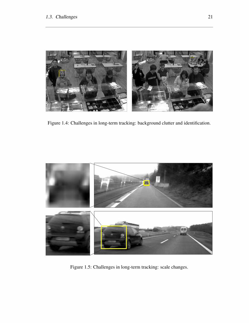
• Scale changes. The object may change scale. While estimation of the scale
can be considered as an implementation detail, it brings an additional degree of
freedom to the tracking process and as such increases vulnerability of the tracker
to failure. The long-term tracker should be able to estimate the scale of an object
as illustrated in figure 1.5.

20 Chapter 1. Introduction
Figure 1.2: Challenges in long-term tracking: occlusion and disappearance.
Figure 1.3: Challenges in long-term tracking: appearance and viewpoint changes.
• Illumination changes. The object changes its appearance under different illumi-
nation. The long-term tracker should be able to deal with illumination changes
as illustrated in figure 1.6.
• Image noise. Video sequences may be corrupted by motion blur, interlacing or
video compression. This influences the accuracy of features that are extracted
from every frame, which may corrupt the output of the tracking algorithm. The
long-term tracker should deal with image noise. Figure 1.7 illustrates the object
corrupted by motion blur.
• Real-time performance. To be useful for interactive applications, the long-
term tracker should work at full frame rate. Therefore, the algorithm must be
extremely efficient.
1.3. Challenges 21
Figure 1.4: Challenges in long-term tracking: background clutter and identification.
Figure 1.5: Challenges in long-term tracking: scale changes.

22 Chapter 1. Introduction
Figure 1.6: Challenges in long-term tracking: illumination changes. All images have
been equalized.
Figure 1.7: Challenges in long-term tracking: motion blur.
1.4 Contributions
This thesis contributes to the research in long-term tracking with the algorithms sum-
marized below.
• TLD framework. We introduce a novel tracking paradigm that decomposes the
long-term tracking task into three sub-tasks: Tracking, Learning and Detection,
each of which is tackled by a dedicated component. The tracker follows the
object from frame to frame. The detector localizes all objects that appear with
appearance that have been observed during tracking and corrects the tracker if
necessary. Exploiting the spatio-temporal structure in the data, the learning com-
ponent estimates errors performed by the detector and updates it to avoid these
errors in the future. The uniqueness of the approach is in the close integration
of all these components which enables mutual compensation of their individual

1.4. Contributions 23
Tracking
Learning
Detectiong
ive
str
aje
ctor
y
givesdete
ction
s
up
da
tes
Figure 1.8: The block diagram of the proposed TLD framework.
flaws. The block diagram of the TLD framework is shown in figure 1.9. The
components of the framework are studied in detail.
• Forward-Backward error. Building on the assumption that correct tracking
is forward-backward consistent, we develop a novel measure that estimates the
reliability of tracking of an arbitrary object in a video stream.
• Median-Flow tracker. We develop an adaptive tracker that is robust to partial
occlusions and deals with appearance and illumination changes. The object of
interest is represented by a bounding box, within which a sparse motion field is
estimated. The reliability of each motion vector is assessed, and the most reliable
vectors determine the motion of the object.
• P-N learning. We develop an unsupervised learning method for online learning
of object detectors from video streams. The learning method is able to learn
an object detector from a single example (defined by a bounding box) and a
video stream where the object may appear. The learning method is formulated
as unsupervised bootstrapping, where the detector errors are estimated by a pair
of “experts”: (i) P-expert estimates missed detections, and (ii) N-expert estimates

24 Chapter 1. Introduction
false alarms. Both of these experts are allowed to make errors themselves. The
learning process is modeled as a discrete dynamical system and the conditions
under which the learning guarantees improvement of the detector are found using
stability criteria developed in control theory [Zhou 96, Ogata 09].
• Boosting+Bootstrap. Motivated by long-term tracking of human faces, we de-
velop a novel learning method for training efficient object detectors. The learn-
ing method is based on a fusion of two popular learning approaches: boost-
ing [Freund 97] and bootstrapping [Sung 98]. We formulate bootstrapping as
weighted sampling where the weights are driven by boosting. The optimal sam-
pling strategy is analytically deduced. Extensive experimental evaluation shows
superior performance with respect to commonly used methods. The learning
method is tested on the task of face detection and state-of-the-art performance is
achieved.
• Implementation. We show how to implement the TLD framework . An exten-
sive quantitative evaluation shows a significant improvement over state-of-the-
art systems. Furthermore, we show how to adapt TLD for face tracking, which
combines an offline trained face detector with online face identification.
1.5 Thesis outline
The structure of the thesis is outlined in figure 1.9. In chapter 2, we review the work
related to long-term tracking from three points of view: object tracking, object detec-
tion and machine learning. In object tracking and object detection, we give special
attention to methods that represent the object by a bounding box. In object learning,
we focus on methods for training of sliding window-based detectors.
Chapters 3, 4 and 5 consider the tracking, learning and detection problems indepen-
dently and propose the basic components of TLD that will be tightly integrated later.

1.5. Thesis outline 25
1. Introduction
3. Tracking
4. Detection
5. Learning
7. Conclusions6. TLD2. Literature Review
Forward-Backward error
Median-Flow tracker
Boosting + Bootstrap
ICPR'10
BMVC'08
CVPR'10
P-N Learning
ICCV'09 (W), ICIP'10
TLD Framework
Figure 1.9: Outline and main contributions of the thesis.
Chapter 3 considers tracking algorithms when applied to unconstrained videos. Ac-
cepting the fact that every tracker eventually fails is the starting point. First, we study
how to detect tracking failures. We define the Forward-Backward error, study its prop-
erties and compare to relevant error measures. Second, we study how the detected
failures can help tracking itself. We develop the Median-Flow tracker and compare it
to state-of-the-art methods on a number of sequences.
Chapter 4 considers offline training of an object detector from large data sets. We
review the algorithms often used for this setting, in particular, boosting [Freund 97]
and bootstrapping [Sung 98]. The optimal combination of boosting and bootstrapping
is developed and evaluated on both synthetic and real data.
Chapter 5 focuses on online learning of an object detector from a single example
and a video stream. The P-N learning theory is developed and formalized as a semi-
supervised [Chapelle 06] learning method. We show how to design a pair of experts
that estimate errors of the detector during learning. We show that tracking can estimate
false negatives and non-maxima-suppression can estimate false positives made by the
detector. The resulting algorithm is quantitatively evaluated on a number of sequences
leading to surprising gains in the detector performance.

26 Chapter 1. Introduction
Chapter 6 develops the TLD framework and describes its implementation. The per-
formance of TLD is evaluated on two types of experiments: (i) tracking of unknown
objects, and (ii) tracking of human faces. A quantitative evaluation is performed on
21 video sequences and compared to 13 relevant tracking algorithms. A significant
improvement over state-of-the-art methods is demonstrated. Furthermore, we perform
a qualitative evaluation and comment on the pros and cons of the proposed approach.
Chapter 7 summarizes the contributions of the thesis, comments on the recent devel-
opments and discusses possible avenues for future research.
1.6 Publications
1. [SUBMITTED] Z. Kalal, K. Mikolajczyk, and J. Matas, ”Tracking-Learning-
Detection,” Transactions on Pattern Analysis and Machine Intelligence, 2010.
2. Z. Kalal, K. Mikolajczyk, and J. Matas, ”Face-TLD: Tracking-Learning-Detection
Applied to Faces,” International Conference on Image Processing, 2010.
3. Z. Kalal, K. Mikolajczyk, and J. Matas, ”Forward-Backward Error: Automatic
Detection of Tracking Failures,” International Conference on Pattern Recogni-
tion, 2010.
4. Z. Kalal, J. Matas, and K. Mikolajczyk, ”P-N Learning: Bootstrapping Binary
Classifiers by Structural Constraints,” Conference on Computer Vision and Pat-
tern Recognition, 2010.
5. Z. Kalal, J. Matas, and K. Mikolajczyk, ”Online Learning of Robust Object De-
tectors During Unstable Tracking,” On-line Learning for Computer Vision Work-
shop, 2009.
6. Z. Kalal, J. Matas, and K. Mikolajczyk, ”Weighted Sampling for Large-Scale
Boosting,” British Machine Vision Conference, 2008.

Chapter 2
Related work
Long-term tracking is a complex problem that is closely related to tracking, detection
and machine learning and in many cases it is studied from one point of view only.
These terms are understood as follows. Tracking estimates the object motion between
consecutive frames relying on temporal coherence in the video. Detection considers
the video frames as independent and localizes all objects that correspond to an object
model. Machine learning is often employed in both of these approaches. Trackers use
machine learning to adapt to changes of the object appearance. Detectors use machine
learning to build better models that cover various appearances of the object.
To give an overview of the most relevant approaches, the chapter is split into four parts.
Section 2.1 gives an overview of tracking approaches ranging from simple template
tracking up to trackers that learn online a discriminative classifier. Section 2.2 reviews
detection approaches focusing on detection of object instances as well as detection
of human faces. Section 2.3 reviews the learning strategies commonly used for the
training of object detectors. In particular we review bootstrapping, boosting as well as
methods based on semi-supervised learning. Section 2.4 comments on observed trends
and outlines challenges that motivated our research.
27
28 Chapter 2. Related work
current object state
Motion estimation
previous object state
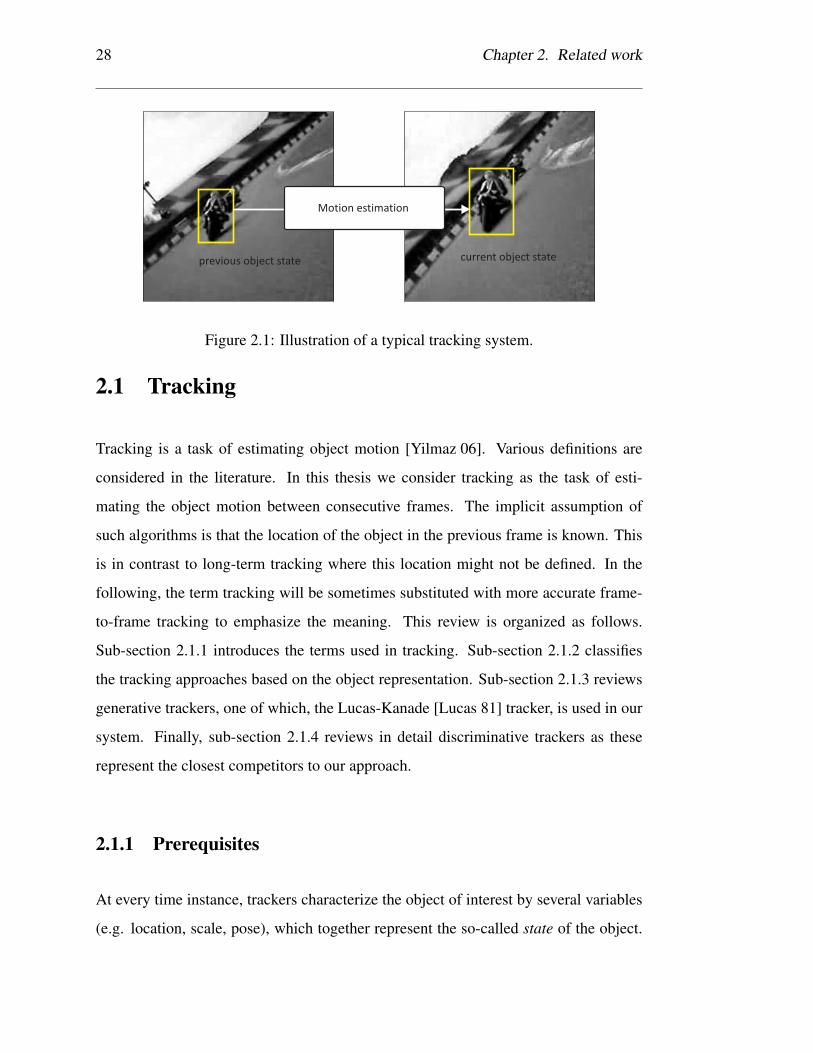
Figure 2.1: Illustration of a typical tracking system.
2.1 Tracking
Tracking is a task of estimating object motion [Yilmaz 06]. Various definitions are
considered in the literature. In this thesis we consider tracking as the task of esti-
mating the object motion between consecutive frames. The implicit assumption of
such algorithms is that the location of the object in the previous frame is known. This
is in contrast to long-term tracking where this location might not be defined. In the
following, the term tracking will be sometimes substituted with more accurate frame-
to-frame tracking to emphasize the meaning. This review is organized as follows.
Sub-section 2.1.1 introduces the terms used in tracking. Sub-section 2.1.2 classifies
the tracking approaches based on the object representation. Sub-section 2.1.3 reviews
generative trackers, one of which, the Lucas-Kanade [Lucas 81] tracker, is used in our
system. Finally, sub-section 2.1.4 reviews in detail discriminative trackers as these
represent the closest competitors to our approach.
2.1.1 Prerequisites
At every time instance, trackers characterize the object of interest by several variables
(e.g. location, scale, pose), which together represent the so-called state of the object.
2.1. Tracking 29
a) b) d)c) e)
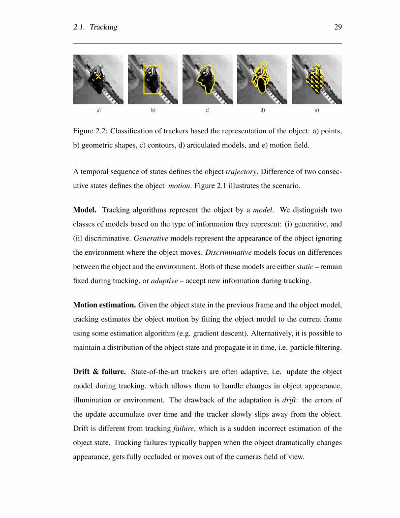
Figure 2.2: Classification of trackers based the representation of the object: a) points,
b) geometric shapes, c) contours, d) articulated models, and e) motion field.
A temporal sequence of states defines the object trajectory. Difference of two consec-
utive states defines the object motion. Figure 2.1 illustrates the scenario.
Model. Tracking algorithms represent the object by a model. We distinguish two
classes of models based on the type of information they represent: (i) generative, and
(ii) discriminative. Generative models represent the appearance of the object ignoring
the environment where the object moves. Discriminative models focus on differences
between the object and the environment. Both of these models are either static – remain
fixed during tracking, or adaptive – accept new information during tracking.
Motion estimation. Given the object state in the previous frame and the object model,
tracking estimates the object motion by fitting the object model to the current frame
using some estimation algorithm (e.g. gradient descent). Alternatively, it is possible to
maintain a distribution of the object state and propagate it in time, i.e. particle filtering.
Drift & failure. State-of-the-art trackers are often adaptive, i.e. update the object
model during tracking, which allows them to handle changes in object appearance,
illumination or environment. The drawback of the adaptation is drift: the errors of
the update accumulate over time and the tracker slowly slips away from the object.
Drift is different from tracking failure, which is a sudden incorrect estimation of the
object state. Tracking failures typically happen when the object dramatically changes
appearance, gets fully occluded or moves out of the cameras field of view.

30 Chapter 2. Related work
2.1.2 Classification
One of the most distinctive properties of a tracking algorithm is the object state, which
determines the variables that are estimated during tracking. Here we use the object
state to classify tracking algorithms into five categories shown in figure 2.2.
1. Points are often used to represent the smallest objects that do not change their
scale dramatically. Algorithms that represent the object by a point will be called
point trackers. Point trackers estimate only translation of the object. The es-
timation can be performed using frame-to-frame tracking [Lucas 81, Shi 94],
key-point matching [Veenman 01], key-point classification [Lepetit 05], or lin-
ear prediction [Zimmermann 09]. Recent work is directed towards optimizing
performance of these methods [Takacs 10].
2. Geometric shapes such as bounding boxes or ellipses, are often used to repre-
sent motion of objects which undergo significant changes in scale. These meth-
ods typically estimate object location, scale and in-plane rotation, all other vari-
ations are typically modeled as the changes of the object appearance.
3. 3D models are used to represent rigid objects, for which the 3D geometry is
known. These models estimate location, scale and pose of the object. These
methods have been applied to various objects including human faces [Vacchetti 04].
A significant effort in tracking is directed towards systems that build the 3D mod-
els online such as SLAM [Davison 03] or PTAM [Klein 07].
4. Contours are used to represent non-rigid objects. Parametric representation of
contours has been used for tracking of human heads [Birchfield 98] or arbitrarily
complex shapes [Isard 98]. Non-parametric representations have been applied
for the tracking of people in sport footage [Yilmaz 04], or various non-rigid ob-
jects including animals and human hands [Bibby 08, Bibby 10].

2.1. Tracking 31
5. Articulated models are used to represent the motion of non-rigid objects con-
sisting of several rigid parts. These models typically consist of several geometric
shapes, for which relative motion is restricted by a model of their geometric re-
lations. Articulated models have been used for tracking of humans [Wang 03,
Ramanan 07] or human arms [Buehler 08].
6. Motion field [Horn 81, Brox 04] is a non-parametric representation of the object
motion which gives the displacement of every pixel of the object between two
frames. An extensive comparison of these methods can be found in [Barron 94].
Recent developments aim at producing long, continuous trajectories of image
points [Sand 08, Goldman 07].
In this thesis we represent the object state by a bounding box. This representation bal-
ances the tradeoff between the expressive power of the representation and the difficulty
to reliably estimate the object motion. The related methods will be now analyzed in
detail.
2.1.3 Generative trackers
Generative trackers model the appearance of the object. In this section we focus on
trackers that represent the object by a geometric shape (i.e. rectangle or ellipse) within
which the appearance is modeled. Motion estimation will be typically formulated as a
search for the best match between an image patch and the model. Even though these
methods were not designed for long-term tracking, we review them as our approach is
relying on number of ideas from this category.
Template tracking
Template trackers represent the object appearance by a single exemplar – a template
(e.g. an image patch). They define a similarity measure between two templates and

32 Chapter 2. Related work
search for such a displacement (or warp) that maximizes the similarity match.
Exhaustive search for the best similarity match is straightforward, but not efficient.
To make it faster, the search can be performed using integral images [Schweitzer 02],
or in frequency domain [Reddy 02]. Another strategy is to restrict the search to the
vicinity of the previous location. Exploration of the neighborhood not only increases
the efficiency of the template tracker, but also reduces the number of false matches.
On the other hand, the tracker may lose the target if the frame-to-frame motion is
larger than expected. In other words, tracker face the tradeoff between speed and
robustness. The most popular strategies for searching within the surrounding of the
previous location are: (i) gradient-based methods, and (ii) mean-shift.
Gradient-based methods optimize the similarity measure using gradient descent. One
of the most popular methods is the Lucas-Kanade [Lucas 81] tracker and its pyramidal
implementation [Bouguet 99], which estimates translation of an image patch. Affine
warping was later proposed in the Kanade-Lucas-Tomasi tracker [Shi 94]. Both of
these approaches have been unified in Inverse Compositional Algorithm [Baker 04].
These methods base the similarity function on SSD. Recently, the similarity func-
tion based on mutual information has been proposed [Dowson 08] which demonstrated
larger convergence basins.
The mean-shift algorithm [Comaniciu 03, Bradski 98] is another approach to avoid the
brute-force search for the best template match. The object is described by a distribution
of colors. Given a new image, every pixel is assigned a probability score from the dis-
tribution resulting in the so-called back-projection image. Mean-shift then iteratively
searches for a mode in the back-projection image. Similarly to the gradient-based
methods, mean-shift cannot handle large displacements as the search is local. On the
other hand, the histogram-based representation handles large appearance changes as
long as the color distribution remains similar.

2.1. Tracking 33
Figure 2.3: The WSL tracker [Jepson 03] estimates components on a template that are
reliable for tracking. This increases the tracker’s robustness to partial occlusion and
appearance changes.
Improvements on template tracking
Template tracking has three main drawbacks. First, template tracking faces a tradeoff
between static and adaptive tracking. A single static template is often not sufficient
to represent all the appearances of the object and adaptation of the template (using
the template from the previous frame) suffers from drift. Second, template tracking is
often sensitive to partial occlusions. Third, a single template does not allow encoding
of multiple appearances.
To tackle the tradeoff between static and adaptive tracking, the basic idea is to adapt
the template only if necessary and re-use the previously observed templates other-
wise. For this purpose a function that evaluates the usefulness of the previously ob-
served templates has to be designed. This idea has been used for tracking of image
patches [Matthews 04, Dowson 05] as well as 3D pose estimation [Rahimi 08].
To tackle the problem of partial occlusions, the WSL tracker [Jepson 03] decomposes
the template into three layers: ”Wandering”, ”Stable” and ”Lost”. It was shown that
by focusing on stable parts of the template, the tracker deals better with partial oc-
clusions and appearance changes. For illustration see figure 2.3. The Fragment-based
tracker [Adam 06] decomposes the template into a set of randomly chosen fragments.
Motion of each fragment is estimated independently and the global motion is estimated
34 Chapter 2. Related work
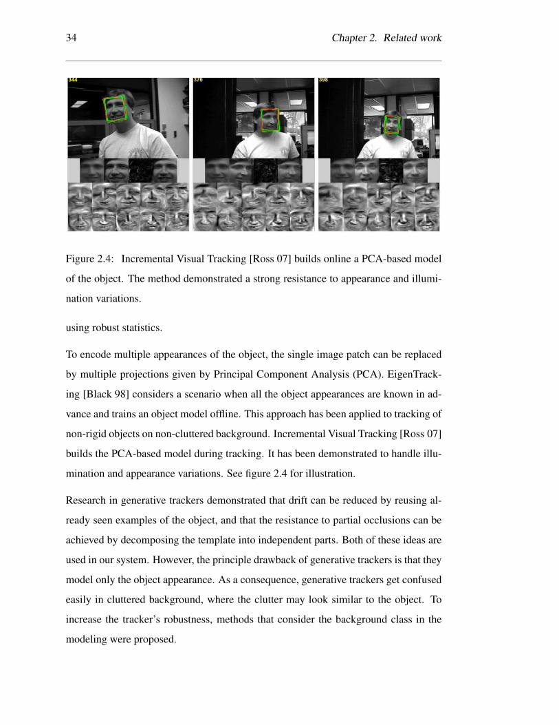
Figure 2.4: Incremental Visual Tracking [Ross 07] builds online a PCA-based model
of the object. The method demonstrated a strong resistance to appearance and illumi-
nation variations.
using robust statistics.
To encode multiple appearances of the object, the single image patch can be replaced
by multiple projections given by Principal Component Analysis (PCA). EigenTrack-
ing [Black 98] considers a scenario when all the object appearances are known in ad-
vance and trains an object model offline. This approach has been applied to tracking of
non-rigid objects on non-cluttered background. Incremental Visual Tracking [Ross 07]
builds the PCA-based model during tracking. It has been demonstrated to handle illu-
mination and appearance variations. See figure 2.4 for illustration.
Research in generative trackers demonstrated that drift can be reduced by reusing al-
ready seen examples of the object, and that the resistance to partial occlusions can be
achieved by decomposing the template into independent parts. Both of these ideas are
used in our system. However, the principle drawback of generative trackers is that they
model only the object appearance. As a consequence, generative trackers get confused
easily in cluttered background, where the clutter may look similar to the object. To
increase the tracker’s robustness, methods that consider the background class in the
modeling were proposed.

2.1. Tracking 35
2.1.4 Discriminative trackers
Discriminative trackers encode the differences between the object appearance and the
environment where the object moves. A common approach is to build a binary clas-
sifier that distinguishes the object from its background. These methods represent the
closest competitors to our system as they often demonstrate re-detection capabilities.
Static discriminative trackers
One of the earliest discriminative trackers was proposed by Avidan [Avidan 04], who
integrated an offline trained SVM classifier into the tracking process. The motion was
estimated by maximizing the classifier confidence using gradient-ascent. The perfor-
mance was demonstrated on the task of vehicle tracking. The main limitation of static
discriminative trackers is in the training data, since all appearances of the object and
background have to be captured in advance.
Adaptive discriminative trackers
Adaptive discriminative trackers learn the discriminative classifier during tracking.
This allows them to track a wide range of objects immediately after initialization.
These trackers typically operate as follows. In the first frame, the tracker builds a
simple classifier separating the selected object from its background. The tracking then
proceeds in a frame-by-frame fashion. In every frame, the classifier is evaluated on the
surrounding of the previous object location and the new location is established, e.g. by
taking the maximally confident location. The tracker then performs an update. The
current location of the object is used to sample positive examples, and the surrounding
is used to sample negative examples of the object appearance. These labeled examples
update the classifier, which is then used in the next frame.
One of the earliest works from this category was by Collins et al. [Collins 05] who

36 Chapter 2. Related work
Figure 2.5: Ensemble tracking [Avidan 07] represents the object of interest by a dis-
criminative model classifying every pixel as the object or background. The classifier
is adapted in every frame. The tracker demonstrated the ability to handle appearance
changes in presence of cluttered environment.
Figure 2.6: The SemiBoost tracker [Grabner 08] reduces drift of discriminative track-
ers by guiding the update by an offline trained classifier. Performance was demon-
strated (among others) on: (TOP) 24h tracking of a still object by static camera, (BOT-
TOM) re-detection of a stationary object after a brief occlusion.

2.1. Tracking 37
built a generative model by discriminative training. The object model, based on color
projections, was adapted during tracking which made it robust to significant illumi-
nation variations. Ensemble Tracking [Avidan 07] updates a boosting-based classifier
to discriminate between pixels on the object and pixels on the background. Online
Boosting [Grabner 06] applies the same principle to a grid of overlapping bounding
boxes instead of individual pixels. Their classifier was based on a set of Haar-like
features [Viola 01] and was trained in an online boosting [Oza 05] framework.
The research in adaptive discriminative tracking has enabled tracking of objects that
significantly change appearance and move in cluttered background. The speed of adap-
tation of the classifier plays an important role in these systems. It controls the impact
of new appearances on the classifier, but also the speed by which the old information is
forgotten. If the speed of adaptation is set correctly for a given problem, these trackers
demonstrate robustness to short-term occlusion. On the other hand, if the object is not
visible for longer time than expected, the tracker will eventually forget the relevant
information and never recover.
Constrained adaptation for discriminative trackers
This section reviews the discriminative tracking approaches that perform constrained
adaptation of the classifier, which is in contrast to every-frame-update reviewed in
the previous sub-section. The constrained adaptation aims at drift reduction as well
as long-term tracking resistant to long-lasting full occlusions. Three classes of ap-
proaches can be identified: (i) semi-supervised learning, (ii) multiple-instance learn-
ing, and (iii) co-training.
Semi-Supervised Learning (SSL) [Chapelle 06] is a learning approach that learns from
both labeled and unlabeled training data. SSL has been applied to a number of prob-
lems in machine learning [Blum 98] and recently also to adaptive discriminative track-
ing. Semi-supervised Online Boosting [Grabner 08] is one of the earliest approaches.

38 Chapter 2. Related work
The initializing frame is considered as a collection of labeled examples, all the re-
maining frames from the sequence are considered as unlabeled. The method employs
two classifiers: (i) a classifier used for tracking, and (ii) an auxiliary classifier used
for update. In the first frame, both classifiers are trained using the labeled data. Dur-
ing the tracking, the auxiliary classifier remained fixed and provides soft-labels to the
unlabeled patches, which are then used to update the tracking classifier. The method
demonstrated reduction of drift and certain re-detection capabilities. See figure 2.6 for
an illustration. Beyond Semi-supervised Online Boosting [Stalder 09] extended the
approach with one more auxiliary classifier to increase the adaptability of the system.
Multiple Instance Learning (MIL) [Dietterich 97] is a variant of supervised learning,
where examples are delivered in groups. Within each group, the examples share the
same label. MILTrack [Babenko 09] combines Online Boosting [Grabner 06] and
MIL. In contrast to the every-frame update, the classifier is updated by spatially re-
lated groups of patches. The introduction of this spatial-information reduced drift
and improved accuracy. Later on, a combination of MILTrack and SSL was pro-
posed [Zeisl 10].
Co-training [Blum 98] is a specific instance of SSL methods, which trains in paral-
lel two independent classifiers. Confident predictions of one classifier train the second
classifier and vice versa. The idea behind the co-trained trackers is the following. If the
object disappears from the view, neither of the classifiers is confident and the update
does not take place. The co-trained Support Vector Machine tracker [Tang 07] repre-
sents the object in two feature spaces (color, gradient orientations [Dalal 05]), which
were used to train two online-SVM [Cauwenberghs 01] classifiers. The co-trained
Generative and Discriminative tracker [Yu 08] exploited the same idea while training
a pair of a generative and a discriminative classifiers. A significant improvement in
re-detection capability with respect to adaptive discriminative trackers was achieved.
In addition, the task of robust object tracking is often studied in offline setting. It
has been shown [Buchanan 06] that points can be tracked very robustly and accurately
2.2. Detection 39
Offline training
Detection
Object Model (classifier)
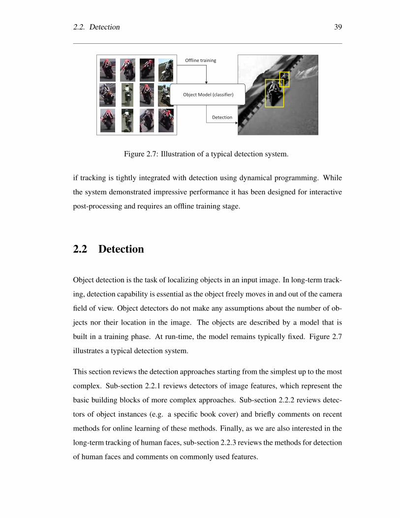
Figure 2.7: Illustration of a typical detection system.
if tracking is tightly integrated with detection using dynamical programming. While
the system demonstrated impressive performance it has been designed for interactive
post-processing and requires an offline training stage.
2.2 Detection
Object detection is the task of localizing objects in an input image. In long-term track-
ing, detection capability is essential as the object freely moves in and out of the camera
field of view. Object detectors do not make any assumptions about the number of ob-
jects nor their location in the image. The objects are described by a model that is
built in a training phase. At run-time, the model remains typically fixed. Figure 2.7
illustrates a typical detection system.
This section reviews the detection approaches starting from the simplest up to the most
complex. Sub-section 2.2.1 reviews detectors of image features, which represent the
basic building blocks of more complex approaches. Sub-section 2.2.2 reviews detec-
tors of object instances (e.g. a specific book cover) and briefly comments on recent
methods for online learning of these methods. Finally, as we are also interested in the
long-term tracking of human faces, sub-section 2.2.3 reviews the methods for detection
of human faces and comments on commonly used features.

40 Chapter 2. Related work
2.2.1 Detection of image features
Feature detectors [Tuytelaars 07] are algorithms that are used to localize salient points
(or regions) in an input image. We distinguish two approaches for feature detection.
Designed detectors. These detectors design a saliency measure and localize features
that maximize it. The widely known approaches are Harris [Harris 88] or Shi-Tomasi
detector [Shi 94], which localize image points. These detectors have been extended to
scale and affine covariant region detectors with the Hessian-Laplace [Mikolajczyk 05]
detector. Other examples from this category are Difference of Gaussians (DoG) [Lowe 04]
or Maximally Stable Extremal Regions (MSER) [Matas 04].
Learned detectors. Feature detection has reached a level of maturity and the re-
search was directed toward proposing more efficient solutions that stem from machine
learning community. A popular algorithm is FAST [Rosten 06] keypoint detector,
which approximates the Harris corner detector [Harris 88]. Efficient approximations
of Hessian-Laplace [Mikolajczyk 05] were also proposed [Sochman 09].
2.2.2 Detection of object instances
This section focuses on methods that detect object instances, such as a specific book
cover. We distinguish approaches which model the object appearance (i) globally and
(ii) locally. We also mention methods for the learning of these detector.
Global appearance models typically represent the object appearance by a collection
of examples and define the detection (and the pose estimation) as the search for the
most similar example in the database. In one of the earliest works, Murase and Na-
yar [Murase 95] use a controlled capturing process to collect a large number of exam-
ples of various 3D objects. Similar idea underpins more recent methods for detection
and rectification of patches [Hinterstoisser 09] or detection of texture-less objects us-
ing dominant orientation templates [Hinterstoisser 10]. Global appearance models are
2.2. Detection 41
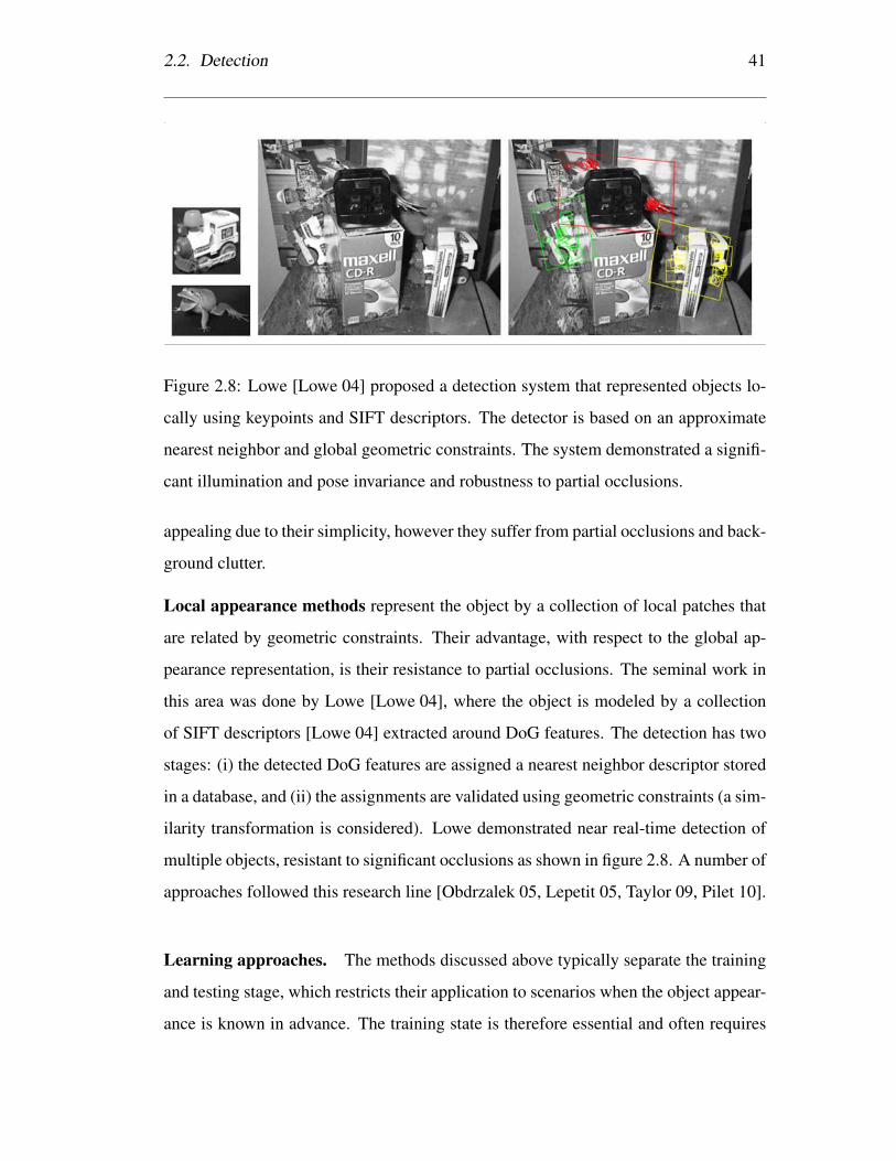
Figure 2.8: Lowe [Lowe 04] proposed a detection system that represented objects lo-
cally using keypoints and SIFT descriptors. The detector is based on an approximate
nearest neighbor and global geometric constraints. The system demonstrated a signifi-
cant illumination and pose invariance and robustness to partial occlusions.
appealing due to their simplicity, however they suffer from partial occlusions and back-
ground clutter.
Local appearance methods represent the object by a collection of local patches that
are related by geometric constraints. Their advantage, with respect to the global ap-
pearance representation, is their resistance to partial occlusions. The seminal work in
this area was done by Lowe [Lowe 04], where the object is modeled by a collection
of SIFT descriptors [Lowe 04] extracted around DoG features. The detection has two
stages: (i) the detected DoG features are assigned a nearest neighbor descriptor stored
in a database, and (ii) the assignments are validated using geometric constraints (a sim-
ilarity transformation is considered). Lowe demonstrated near real-time detection of
multiple objects, resistant to significant occlusions as shown in figure 2.8. A number of
approaches followed this research line [Obdrzalek 05, Lepetit 05, Taylor 09, Pilet 10].
Learning approaches. The methods discussed above typically separate the training
and testing stage, which restricts their application to scenarios when the object appear-
ance is known in advance. The training state is therefore essential and often requires

42 Chapter 2. Related work
Figure 2.9: Feature harvesting [Ozuysal 06], a method for automatic training of an
object detector in a controlled environment (TOP). After the training phase the detector
operates in cluttered environments (BOTTOM).
a large number of human-annotated training examples. In order to simplify the train-
ing stage, Feature Harvesting [Ozuysal 06] learns the geometry and the appearance of
an object automatically from a video. The method assumes a rigid 3D object moving
slowly in a video sequence. After the training phase, the algorithm is able to detect
the object and estimate its 3D pose in a cluttered background. See figure 2.9 for il-
lustration. Another direction is to make the training instantaneous and thus remove
the difference between training and run-time. A common strategy is to simply add
new templates [Hinterstoisser 10] or to integrate new views into the classifier exploit-
ing the computation performed in the offline training [Calonder 08, Hinterstoisser 09,
Pilet 10].
For certain classes of objects, the detection of object instances has reached a level of
maturity. In particular, planar and textured objects can be reliably detected in real-time
and are often used in augmented reality applications. Objects that are non-rigid and
non-textured still remain challenging for detection. With respect to online learning,
several methods are designed to enable instantaneous online learning, but the decision
when to learn new appearances is not directly addressed.

2.2. Detection 43
d) sliding window
background
face
c) cascaded-classifier e) non-maximum suppresionb) features
...
a) training set
...
Figure 2.10: Illustration of a typical face detection components.
2.2.3 Detection of faces
Face detection is a task of localizing of human faces in an input image, regardless
of their pose, illumination, expression or identity. This section briefly mentions the
history of face detection, describes the most popular approaches and comments on the
commonly used features.
History. Research in face detection started in early 70’ with approaches that modeled
the face appearance by a set of rules provided by the researcher [Fischler 73, Sinha 94].
This view was mainly motivated by the ease with which rules could be designed
(e.g. a face has two eyes) and the lack of computational resources that would enable
learning of these rules explicitly. With increasing computational capacity, learning-
based methods started to dominate in 90’, which learn the rules from training ex-
amples [Turk 91, Belhumeur 97, Osuna 97, Sung 98, Rowley 98, Papageorgiou 98].
While a number of these approaches achieved high detection rates [Schneiderman 04],
their practical applicability was limited due to their speed. This was changed by Vi-
ola and Jones [Viola 01] approach, who introduced the first real-time face detector.
Since then, research in face detection iterates over the Viola and Jones approach [Li 04,
Fleuret 01, Jones 03, Sochman 05, Huang 07] and is often considered as solved.
Viola and Jones face detector combined a number of techniques previously developed
in face detection. Many of these techniques reach beyond face detection and are used
in our long-term tracking system as well. Refer to the figure 2.10.

44 Chapter 2. Related work
• Training set. The face is represented by a model, which is learned from a large
collection of labeled training examples. The positive examples depict tightly
cropped faces, negative examples depict non-faces.
• Local features. The training examples are described by local features. Popular
features are Haar wavelets [Papageorgiou 98] which encode intensity patterns.
The features are efficiently measured using integral images [Viola 01].
• Cascaded classifiers. The face model has a form of a binary classifier which is
split into a number of stages. Every stage enabled early rejection of background
examples. This cascaded architecture, which leads to a significant increase of
the classification speed, was first used in [Yang 94].
• Sliding window. The cascaded classifier is evaluated on a grid of locations at
multiple scales. At every location, the classifier decides about presence or ab-
sence of the face.
• Non-maximum suppression. Due to the sliding window approach, the classifier
typically produces multiple overlapping responses around the face. A common
approach is to take the locally maximal confidence response and suppress all the
remaining responses.
• Boosting+Bootstrap. The classifier is typically learned using a combination of
boosting [Freund 97] and bootstrapping [Sung 98]. As one of the contribution
of this thesis is the optimal combination of these methods. A detailed review of
these methods is given in section 2.3.
Features used in object detection. Features play an important role in object detection
as they encode our knowledge about the object. Here we give a brief overview of
features that are commonly used for description of object appearance. See figure 2.11
for an illustration.
2.2. Detection 45
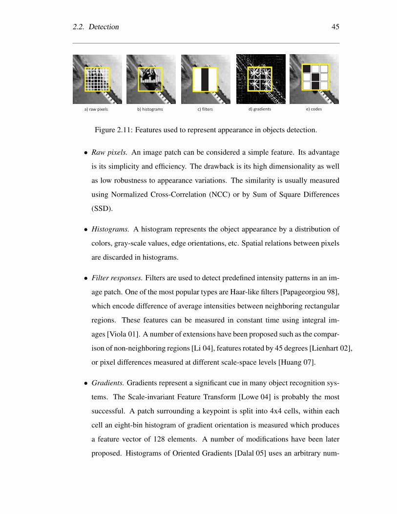
b) histograms c) filters d) gradients e) codesa) raw pixels
Figure 2.11: Features used to represent appearance in objects detection.
• Raw pixels. An image patch can be considered a simple feature. Its advantage
is its simplicity and efficiency. The drawback is its high dimensionality as well
as low robustness to appearance variations. The similarity is usually measured
using Normalized Cross-Correlation (NCC) or by Sum of Square Differences
(SSD).
• Histograms. A histogram represents the object appearance by a distribution of
colors, gray-scale values, edge orientations, etc. Spatial relations between pixels
are discarded in histograms.
• Filter responses. Filters are used to detect predefined intensity patterns in an im-
age patch. One of the most popular types are Haar-like filters [Papageorgiou 98],
which encode difference of average intensities between neighboring rectangular
regions. These features can be measured in constant time using integral im-
ages [Viola 01]. A number of extensions have been proposed such as the compar-
ison of non-neighboring regions [Li 04], features rotated by 45 degrees [Lienhart 02],
or pixel differences measured at different scale-space levels [Huang 07].
• Gradients. Gradients represent a significant cue in many object recognition sys-
tems. The Scale-invariant Feature Transform [Lowe 04] is probably the most
successful. A patch surrounding a keypoint is split into 4x4 cells, within each
cell an eight-bin histogram of gradient orientation is measured which produces
a feature vector of 128 elements. A number of modifications have been later
proposed. Histograms of Oriented Gradients [Dalal 05] uses an arbitrary num-
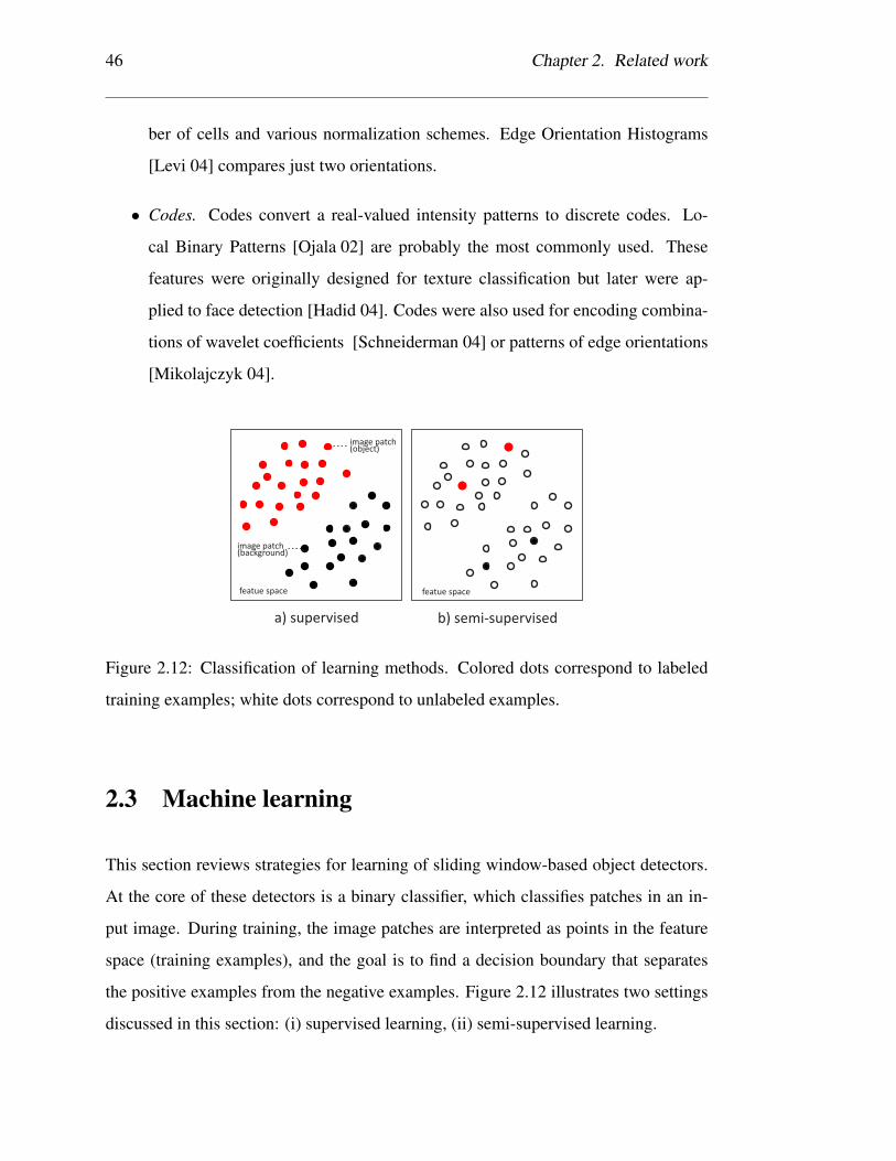
46 Chapter 2. Related work
ber of cells and various normalization schemes. Edge Orientation Histograms
[Levi 04] compares just two orientations.
• Codes. Codes convert a real-valued intensity patterns to discrete codes. Lo-
cal Binary Patterns [Ojala 02] are probably the most commonly used. These
features were originally designed for texture classification but later were ap-
plied to face detection [Hadid 04]. Codes were also used for encoding combina-
tions of wavelet coefficients [Schneiderman 04] or patterns of edge orientations
[Mikolajczyk 04].
b) semi-superviseda) supervised
featue space featue space
image patch(object)
image patch(background)
Figure 2.12: Classification of learning methods. Colored dots correspond to labeled
training examples; white dots correspond to unlabeled examples.
2.3 Machine learning
This section reviews strategies for learning of sliding window-based object detectors.
At the core of these detectors is a binary classifier, which classifies patches in an in-
put image. During training, the image patches are interpreted as points in the feature
space (training examples), and the goal is to find a decision boundary that separates
the positive examples from the negative examples. Figure 2.12 illustrates two settings
discussed in this section: (i) supervised learning, (ii) semi-supervised learning.
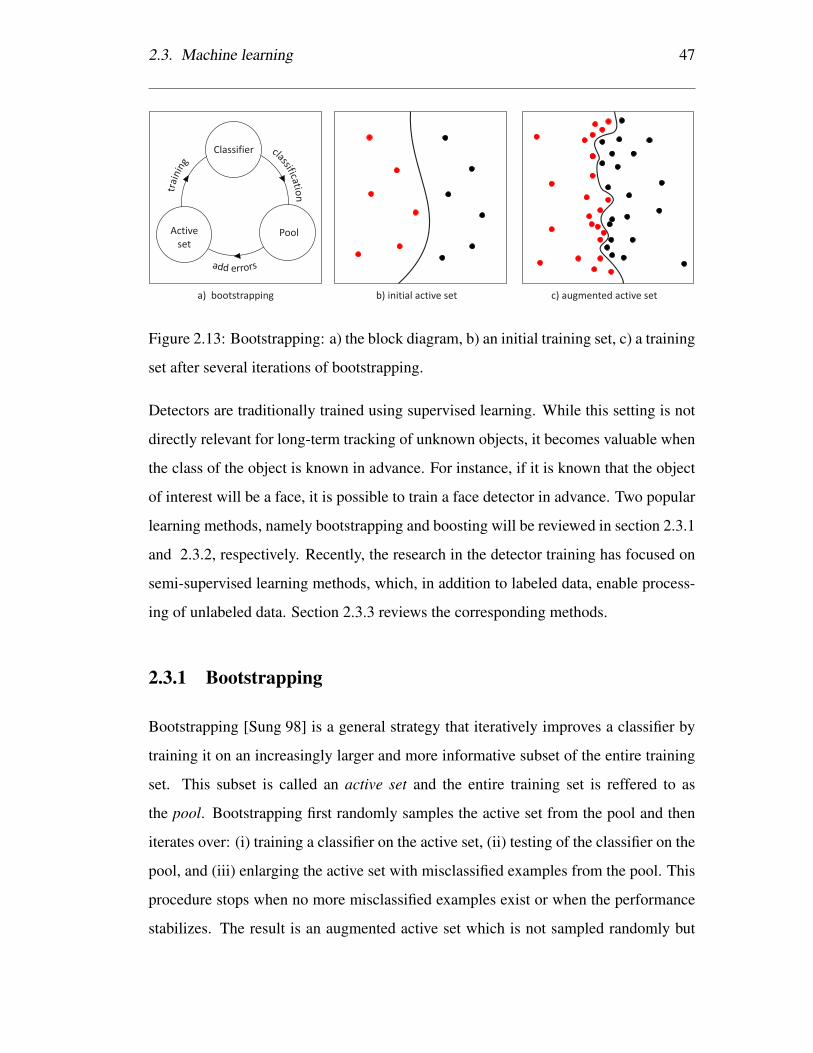
2.3. Machine learning 47
Active
set
Classifier
Pool
add errors
a) bootstrapping b) initial active set c) augmented active set
Figure 2.13: Bootstrapping: a) the block diagram, b) an initial training set, c) a training
set after several iterations of bootstrapping.
Detectors are traditionally trained using supervised learning. While this setting is not
directly relevant for long-term tracking of unknown objects, it becomes valuable when
the class of the object is known in advance. For instance, if it is known that the object
of interest will be a face, it is possible to train a face detector in advance. Two popular
learning methods, namely bootstrapping and boosting will be reviewed in section 2.3.1
and 2.3.2, respectively. Recently, the research in the detector training has focused on
semi-supervised learning methods, which, in addition to labeled data, enable process-
ing of unlabeled data. Section 2.3.3 reviews the corresponding methods.
2.3.1 Bootstrapping
Bootstrapping [Sung 98] is a general strategy that iteratively improves a classifier by
training it on an increasingly larger and more informative subset of the entire training
set. This subset is called an active set and the entire training set is reffered to as
the pool. Bootstrapping first randomly samples the active set from the pool and then
iterates over: (i) training a classifier on the active set, (ii) testing of the classifier on the
pool, and (iii) enlarging the active set with misclassified examples from the pool. This
procedure stops when no more misclassified examples exist or when the performance
stabilizes. The result is an augmented active set which is not sampled randomly but
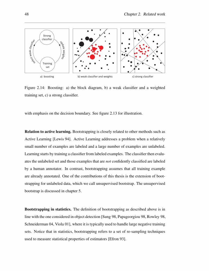
48 Chapter 2. Related work
Strong
classifier
Training
set
a) boosting b) weak classifier and weights c) strong classifier
Figure 2.14: Boosting: a) the block diagram, b) a weak classifier and a weighted
training set, c) a strong classifier.
with emphasis on the decision boundary. See figure 2.13 for illustration.
Relation to active learning. Bootstrapping is closely related to other methods such as
Active Learning [Lewis 94]. Active Learning addresses a problem when a relatively
small number of examples are labeled and a large number of examples are unlabeled.
Learning starts by training a classifier from labeled examples. The classifier then evalu-
ates the unlabeled set and those examples that are not confidently classified are labeled
by a human annotator. In contrast, bootstrapping assumes that all training example
are already annotated. One of the contributions of this thesis is the extension of boot-
strapping for unlabeled data, which we call unsupervised bootstrap. The unsupervised
bootstrap is discussed in chapter 5.
Bootstrapping in statistics. The definition of bootstrapping as described above is in
line with the one considered in object detection [Sung 98, Papageorgiou 98, Rowley 98,
Schneiderman 04, Viola 01], where it is typically used to handle large negative training
sets. Notice that in statistics, bootstrapping refers to a set of re-sampling techniques
used to measure statistical properties of estimators [Efron 93].

2.3. Machine learning 49
2.3.2 Boosting
Boosting [Freund 97] is a supervised learning strategy which aims to improve the per-
formance of a weak classifier. The intuition behind boosting is: focus on the most
difficult training examples. This is achieved by maintaining a distribution of example
weights that represent the example’s difficulty. This section briefly comments on the
history of boosting, its relation to ensemble methods and links to bootstrapping.
Consider a labeled training set and a set of arbitrary weak classifiers. Boosting com-
bines these weak classifiers into a strong classifier which performs better than any of
the weak classifiers. Boosting is an iterative process which iterates over: (i) selection
of the weak classifier that performs best on current distribution of weights, and (ii)
the update of the distribution to emphasize misclassified examples. The set of weak
classifiers selected in each round form the strong classifier. Boosting methods differ in
the way the example weights are updated, which depends on a particular loss function.
A common property of all of boosting methods is that a weak classifier selected in
iteration k has 50% error in iteration k+ 1 which prevents it being selected again. The
block diagram of boosting, a weak classifier and a strong classifier are illustrated in
figure 2.14.
History. Boosting has been studied for two decades now. Schapire [Schapire 90] de-
veloped the first boosting procedure that could always improve the performance of
a classifier by training two additional classifiers on modified versions of the training
data. One year later, Freund [Freund 95] generalized the algorithm to combine an ar-
bitrary number of weak classifiers. Both of these versions assume weak classifiers
which have identical error rates. This assumption was dropped by the discrete Ad-
aBoost [Freund 97] algorithm, which enabled to boost classifiers with arbitrary error
rates. The strong classifier was defined as weighted majority vote. In a comparative
study, Quinlan [Quinlan 96] observed that trees can be boosted into more accurate
classifier if each node outputs a confidence value rather than a discrete class. Sub-

50 Chapter 2. Related work
sequently, real AdaBoost [Schapire 98b] was proposed, which allowed the classifier
to output confidences and achieved a significant improvement in classification over
discrete AdaBoost.
Improvements of boosting. Early versions of Boosting [Schapire 90, Freund 95] used
a stopping criterion for the number of combined weak classifiers to avoid over-fitting.
However, practitioners observed [Schneiderman 04] that testing error keeps decreas-
ing and then stabilizes when the boosting is not terminated. This phenomenon was
explained by the ”margin theory” [Schapire 98a]. Moreover, the performance of boost-
ing was explained from statistical point of view [Friedman 00] as an additive logistic
regression. Boosting algorithms are still evolving. Robustness to noisy data was ad-
dressed by BrownBoost [Freund 01] or LogitBoost [Friedman 00]. An online variant
of boosting have been also proposed [Oza 05]. A comprehensive review of the methods
can be found in [Schapire 02].
Relation to ensemble methods. Boosting has close links to other algorithms which
internally maintain a set of weak classifiers and integrate their responses by majority
voting, i.e. ensemble classifiers. The underlying assumption of these methods is that
the classifiers make independent errors and therefore the majority voting improves
their performance [Polikar 06]. The methods differ in the way the independence of
the classifiers is achieved. Bagging [Breiman 96] uses sampling with repetition to
form different training distributions. If the weak classifiers are trees, bagging becomes
a Randomized Forrest [Breiman 01], which has been applied in computer vision to
a number of problems [Amit 97, Lepetit 05, Shotton 08]. Apart from sampling with
repetition, the classifier independence can be achieved by designing features which
are likely to be independent such as in Randomized Ferns [Ozuysal 07]. A similar
approach is used in our implementation.
Boosting and sliding-windows. Boosting has been developed for general machine
learning problems. However, such algorithm may struggle in some practical scenarios
such as face detection using a sliding window. In a typical image, the sliding-window
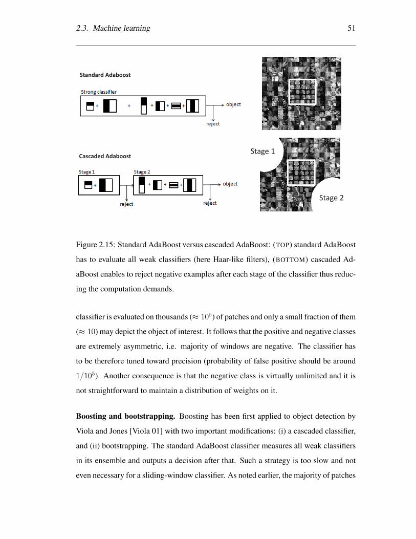
2.3. Machine learning 51
Stage 1
Stage 2
Standard Adaboost
Cascaded Adaboost
Figure 2.15: Standard AdaBoost versus cascaded AdaBoost: (TOP) standard AdaBoost
has to evaluate all weak classifiers (here Haar-like filters), (BOTTOM) cascaded Ad-
aBoost enables to reject negative examples after each stage of the classifier thus reduc-
ing the computation demands.
classifier is evaluated on thousands (≈ 105) of patches and only a small fraction of them
(≈ 10) may depict the object of interest. It follows that the positive and negative classes
are extremely asymmetric, i.e. majority of windows are negative. The classifier has
to be therefore tuned toward precision (probability of false positive should be around
1/105). Another consequence is that the negative class is virtually unlimited and it is
not straightforward to maintain a distribution of weights on it.
Boosting and bootstrapping. Boosting has been first applied to object detection by
Viola and Jones [Viola 01] with two important modifications: (i) a cascaded classifier,
and (ii) bootstrapping. The standard AdaBoost classifier measures all weak classifiers
in its ensemble and outputs a decision after that. Such a strategy is too slow and not
even necessary for a sliding-window classifier. As noted earlier, the majority of patches

52 Chapter 2. Related work
b) unlabeled data c) semi-supervised d) comparison of classifiersa) supervised
Figure 2.16: Can unlabeled data improve a classifier? Refer to the text for explanation.
in a typical image depict background. Therefore the classifier is split into stages, each
of which rejects (classifies as negative) a subset of candidates before progressing to
the next stage. This cascaded structure has a great impact on the classifier speed but
also influences the quality of training. Standard training maintains only a distribution
of weights and considers the training set as fixed. In contrast, training with a cascaded
classifier involves resampling of the training set to better represent the examples close
to the current decision boundary, which has direct links to bootstrapping [Sung 98].
2.3.3 Semi-supervised learning
This section reviews the semi-supervised learning methods, which, in addition to la-
beled examples, exploit unlabeled training examples.
A natural question is whether unlabeled data can help in training of a classifier. Con-
sider the mind experiment illustrated in figure 2.16. The goal is to train a classifier
in two settings: (i) from two labeled examples, and (ii) from the identical labeled ex-
amples and a collection of unlabeled examples. Given the labeled examples only, a
number of supervised methods can be used to train a classifier. Figure 2.16 (a) illus-
trates the decision boundary of a classifier that maximizes the classification margin. If
the labeled examples are augmented by unlabeled (b) several semi-supervised learning
strategies can be used. One of the simplest is to perform clustering of the unlabeled
examples and label each cluster by the corresponding labeled example within it. This

2.3. Machine learning 53
produces a decision boundary that is illustrated in (c). This classifier will make correct
predictions as long as the clustering is aligned with the classification that is demanded
(d). This example demonstrates that if the underlying distribution of unlabeled exam-
ples forms clusters that are aligned with the classification function to be learned, the
unlabeled data can help when training a classifier. This property of unlabeled data, also
referred to as the ”cluster assumption”, is often assumed by the semi-supervised learn-
ing algorithms [Chapelle 06]. A number of algorithms relying on similar assumptions
have been proposed in the past including Expectation-Maximization, self-learning and
co-training.
Expectation-Maximization (EM) is a generic method for finding estimates of model
parameters given unlabeled data. EM is an iterative process, which in case of bi-
nary classification alternates over: (i) estimation of soft-labels of unlabeled data, and
(ii) training a classifier exploiting the soft-labels. EM was successfully applied to
document classification [Nigam 00] and learning of object categories [Fergus 03]. In
the semi-supervised learning terminology, EM algorithm relies on the ”low density
separation” assumption [Chapelle 06], which means that the classes are well sepa-
rated in the feature space. EM is sometimes interpreted as a “soft” version of Self-
learning [Zhu 09].
Self-learning starts by training an initial classifier from a labeled training set, the clas-
sifier is then evaluated on the unlabeled data. The examples with the most confident
classifier responses are added to the training set and the classifier is retrained. This
is an iterative process. Self-learning has been applied to training of a human eye de-
tector [Rosenberg 05]. However, it was observed that the detector improved more if
the unlabeled data was selected by an independent measure rather than the classifier
confidence. Rosenberg et al. suggested that the low density separation assumption is
not satisfied for object detection and other approaches may work better.
Co-training [Blum 98] is a learning method built on the idea that independent classi-
fiers can mutually train one another. To create such independent classifiers, co-training

54 Chapter 2. Related work
Unlabeled dataView 1
Classifier
Training set
train
View 2
Classifier
Training set
trainconfident
examples
classifyconfident
examples
classify
Figure 2.17: Illustration of co-training [Blum 98] of two classifiers.
assumes that two independent feature-spaces are available. See figure 2.17 for illustra-
tion of the process. The training is initialized by the training of two separate classifiers
using the labeled examples. Both classifiers are then evaluated on unlabeled data. The
confidently labeled samples from the first classifier are used to augment the training
set of the second classifier and vice versa in an iterative process. Co-training works
best for problems with independent modalities, e.g. text classification [Blum 98] (text
and hyper-links) or biometric recognition systems [Poh 09] (appearance and voice).
In visual object detection, co-training has been applied to car detection in surveil-
lance [Levin 03] or moving object recognition [Javed 05]. We argue that co-training
is not a good choice for object detections, since the examples (image patches) are
sampled from a single modality. Features extracted from a single modality may be
dependent and therefore violate the assumptions of co-training.

2.4. Observations 55
2.4 Observations
Tracking. We reviewed methods starting from the most basic approaches such as
template tracking, up to complex trackers which define tracking as classification and
update the classifier during tracking. Trackers are becoming increasingly complex to
handle increasingly challenging environments and appearance changes. The assump-
tion is that the object state in the previous frame is known. In unconstrained video, this
assumption is violated and therefore any tracker eventually fails. The tracking failure
will be investigated in chapter 3.
Detection. Object instance detection reached a level of maturity for scenarios where
a sufficient number of training examples can be either generated or annotated. A cas-
caded architecture, or fast keypoint detectors enable tracking-by-detection, which over-
comes the drift and initialization problems of contemporary trackers. The underlying
assumption of object detectors is a separation of training and run-time phase. This lim-
its their applicability to objects that can be modeled in advance. Methods that enable
efficient online update of detectors have been proposed, but the problem how to update
these detectors was not addressed.
Learning. We reviewed two classes of learning approaches for training of object
detectors: supervised and semi-supervised. In the supervised setting the learning is
often realized by boosting. However, the standard variants of boosting, do not per-
form well and have to be combined with bootstrapping to handle large training sets.
Chapter 4 closely analyses this relationship between boosting and bootstrapping and
proposes a unifying algorithm. In the semi-supervised setting we discussed several ap-
proaches popular in text classification, however in object detection the improvements
are marginal. One of the reasons is that in object detection it is hard to find independent
features that would efficiently drive the learning process. Chapter 5 discusses other in-
formation sources (spatio-temporal structure in data) that could be used for training an
object detector.

56 Chapter 2. Related work
Chapter 3
Tracking: failure detection
This chapter investigates long-term tracking from the perspective of frame-to-frame
tracking. The starting point is the observation that any frame-to-frame tracker eventu-
ally fails, for instance, when the object moves out of the camera view. Therefore, the
primary goal of this chapter is to estimate the reliability of a tracker and use it to detect
the tracking failures. The secondary goal is to use the reliability measure to improve
the frame-to-frame tracking itself.
The chapter is structured as follows. Section 3.1 focuses on point trackers and proposes
a novel error measure that evaluates the reliability of arbitrarily long point trajectories.
Section 3.2 develops a novel tracker called Median-Flow. The object is represented by
a grid of points, which influence the estimated object motion based on their reliabil-
ity. The Median-Flow tracker is comparatively evaluated with relevant approaches and
superior performance is achieved. The chapter is concluded in section 3.3.
3.1 Detection of tracking failures
This section is concerned with the detection of tracking failures of point trackers, e.g.
Lucas-Kanade tracker [Lucas 81]. These trackers build up a point trajectory from a
57

58 Chapter 3. Tracking: failure detection
sequence of frame-to-frame displacements. Such trackers are: (i) prone to drift due to
accumulation of localization errors, and (ii) likely to fail if the point suddenly changes
appearance, becomes occluded or disappears from the camera view.
Our approach to failure detection is based on so called forward-backward consistency
assumption that correct tracking should be independent of the direction of time-flow.
Algorithmically, this assumption is exploited as follows. First, a tracker produces a
trajectory by tracking a point forward in time. The trajectory has arbitrary length, and
can be obtained by an arbitrary tracker. Second, the point location in the last frame
of the forward trajectory initializes a validation trajectory. The validation trajectory is
obtained by backward tracking. Third, the two trajectories are compared and if they
differ significantly, the forward trajectory is considered as incorrect.
Figure 3.1 (TOP) illustrates the method when tracking a point between two images
(trajectory of length one). Point no. 1 is visible in both images and the tracker is able
to localize it correctly. Tracking this point forward or backward results in consistent
trajectories. On the other hand, point no. 2 is not visible in the right image and the
tracker localizes a different point. Backward-tracking of this point results in a different
location than the original one. The corresponding forward and backward trajectories
are significantly different in this case.
Related work. A commonly used approach to detect tracking failures is to compare
consecutive point-centered patches using Sum of Square Differences (SSD) [Bouguet 99,
Nickels 02]. High SSD means that the patches are dissimilar, which indicates tracking
failure. This differential error indicates failures caused by occlusion or rapid move-
ments, but does not detect slowly drifting trajectories. The detection of drift can be ap-
proached by defining an absolute error. A popular approach is to consider affine warps
of the initial patch [Shi 94] and compare them to the current patch. Recently, a general
method for assessing the tracking performance was proposed [Wu 07, Dowson 06],
which is based on the “forward-backward” idea. The forward-backward consistency

3.1. Detection of tracking failures 59
Figure 3.1: Illustration of the Forward-Backward error measure: (TOP) consistent (1)
and inconsistent (2) trajectories, (BOTTOM) terms used for the definition of the
Forward-Backward error measure.
was used to automatically evaluate the tracking performance without the need to de-
fine the ground truth manually. Improvement of the tracking performance based on
the forward-backward consistency was not considered. Moreover, the idea of forward-
backward consistency is often used wide-baseline matching [Strecha 03] or in optical
flow estimation [Alvarez 07]. These methods typically consider a pair of images. In
contrast, our approach defines the error for arbitrarily long point trajectories.
3.1.1 Forward-Backward error
This section defines the Forward-Backward (FB) error, see figure 3.1 (BOTTOM) for
illustration. Let (It, It+1..., It+k) be an image sequence and pt be a point location in
time t. Using an arbitrary tracker, the point pt is tracked forward for k steps. The
resulting trajectory is−→T k = (pt, pt+1, ..., pt+k). Our goal is to estimate the reliability
of trajectory−→T k given the image sequence. For this purpose, the validation trajectory
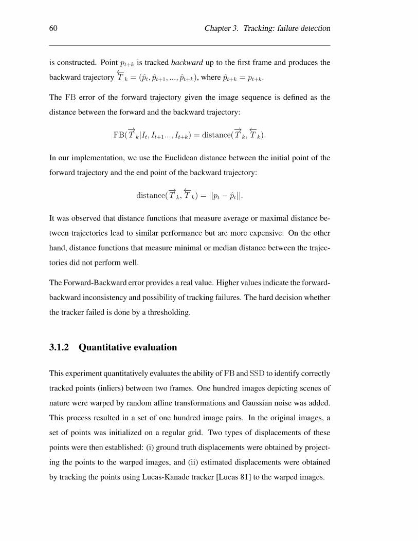
60 Chapter 3. Tracking: failure detection
is constructed. Point pt+k is tracked backward up to the first frame and produces the
backward trajectory←−T k = (pt, pt+1, ..., pt+k), where pt+k = pt+k.
The FB error of the forward trajectory given the image sequence is defined as the
distance between the forward and the backward trajectory:
FB(−→T k|It, It+1..., It+k) = distance(
−→T k,←−T k).
In our implementation, we use the Euclidean distance between the initial point of the
forward trajectory and the end point of the backward trajectory:
distance(−→T k,←−T k) = ||pt − pt||.
It was observed that distance functions that measure average or maximal distance be-
tween trajectories lead to similar performance but are more expensive. On the other
hand, distance functions that measure minimal or median distance between the trajec-
tories did not perform well.
The Forward-Backward error provides a real value. Higher values indicate the forward-
backward inconsistency and possibility of tracking failures. The hard decision whether
the tracker failed is done by a thresholding.
3.1.2 Quantitative evaluation
This experiment quantitatively evaluates the ability of FB and SSD to identify correctly
tracked points (inliers) between two frames. One hundred images depicting scenes of
nature were warped by random affine transformations and Gaussian noise was added.
This process resulted in a set of one hundred image pairs. In the original images, a
set of points was initialized on a regular grid. Two types of displacements of these
points were then established: (i) ground truth displacements were obtained by project-
ing the points to the warped images, and (ii) estimated displacements were obtained
by tracking the points using Lucas-Kanade tracker [Lucas 81] to the warped images.
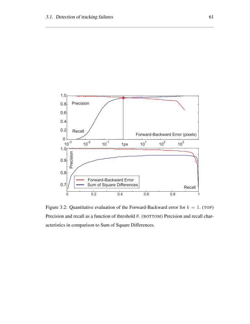
3.1. Detection of tracking failures 61
10-3
10-2
10-1
1px 101
102
103
0
0.2
0.4
0.6
0.8
1.0
Forward-Backward Error (pixels)Recall
Precision
0 0.2 0.4 0.6 0.8 1
0.7
1.0
Recall
Pre
cis
ion
0.8
0.9
Forward-Backward ErrorSum of Square Differences
Figure 3.2: Quantitative evaluation of the Forward-Backward error for k = 1. (TOP)
Precision and recall as a function of threshold θ. (BOTTOM) Precision and recall char-
acteristics in comparison to Sum of Square Differences.

62 Chapter 3. Tracking: failure detection
The estimated displacements that ended up closer than 2 pixels from the ground truth
were labeled as inliers. We selected the threshold of 2 pixels since Lucas-Kanade does
not estimate affine deformation and with too tight threshold, the majority of points
would be classified as outliers. By setting the threshold to 2 pixels we are interested
in recognition of catastrophic tracking failures. Affine deformation and the Gaussian
noise are used as approximations of real variations of the point appearance.
Using the 2 pixel threshold, the inliers represented approximately 65% of all displace-
ments. The estimated displacements were then evaluated by a failure detection mea-
sure (FB, SSD), displacements with error below θ were classified as inliers. A correct
classification of an inlier is denoted as a true positive (TP), an incorrect classification
is denoted as false positive (FP). The quality of the error measures is accessed using
precision and recall statistics, which are both function of threshold θ:
precision =TP
TP + FP, recall =
TP
#inliers.
Figure 3.2 (TOP) shows the resulting performance of the FB error as a function of
the threshold θ. The figure illustrates that the proposed FB error is able to reliably
recognize majority of inliers at high precision level. Notice for instance the working
point indicated by the red dot. For θ = 1 pixel, the recall is of 95% and precision of
96%. Figure 3.2 (BOTTOM) shows the corresponding precision and recall curves for
FB in comparison to SSD. FB outperforms SSD for majority of working points. SSD
was unable to detect inliers for small thresholds, its precision starts below 70% (notice
that random guessing would start around 65%).
3.1.3 Visualization
This sub-section visualizes the proposed Forward-Backward error for long point tra-
jectories. Given a video sequence, every pixel in the first frame initializes a point
trajectory. Every point is tracked forward up to the last frame and then backward up
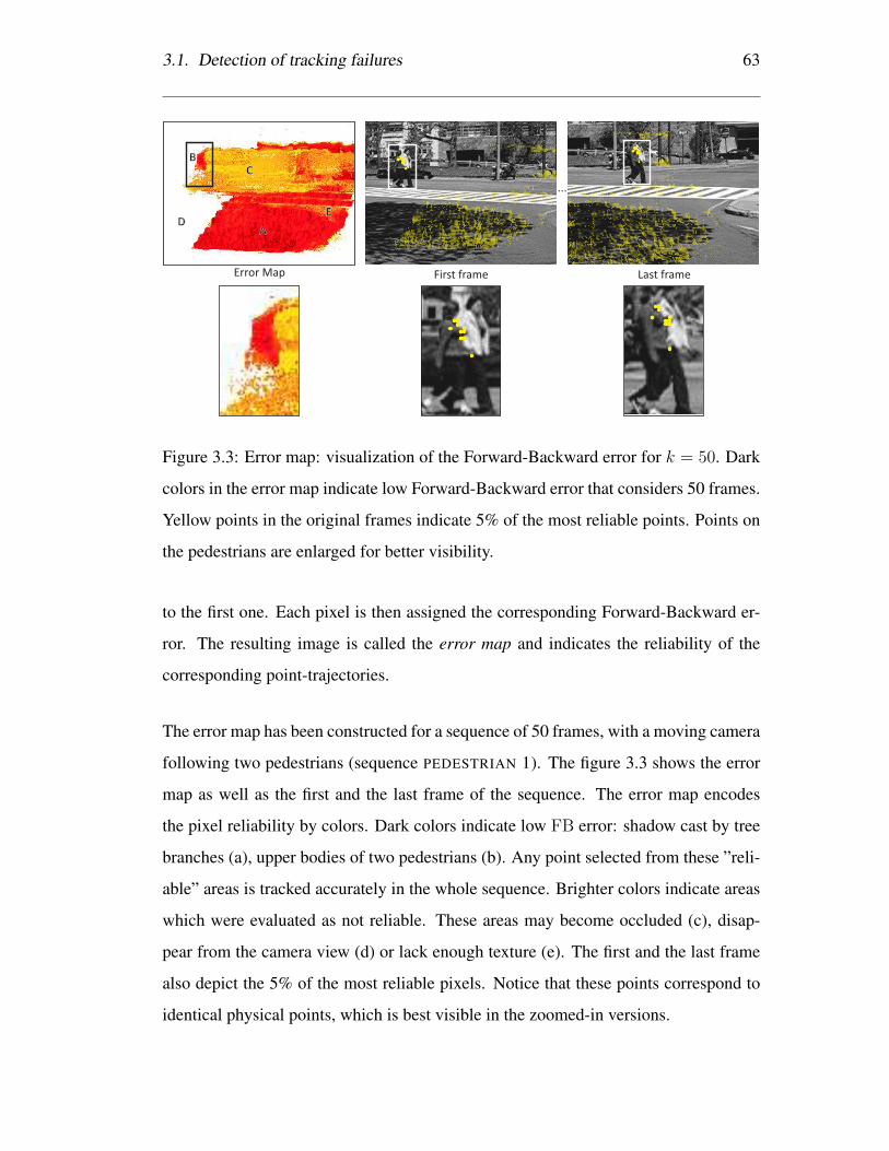
3.1. Detection of tracking failures 63
Error Map First frame Last frame
...
A
B
C
DE
Figure 3.3: Error map: visualization of the Forward-Backward error for k = 50. Dark
colors in the error map indicate low Forward-Backward error that considers 50 frames.
Yellow points in the original frames indicate 5% of the most reliable points. Points on
the pedestrians are enlarged for better visibility.
to the first one. Each pixel is then assigned the corresponding Forward-Backward er-
ror. The resulting image is called the error map and indicates the reliability of the
corresponding point-trajectories.
The error map has been constructed for a sequence of 50 frames, with a moving camera
following two pedestrians (sequence PEDESTRIAN 1). The figure 3.3 shows the error
map as well as the first and the last frame of the sequence. The error map encodes
the pixel reliability by colors. Dark colors indicate low FB error: shadow cast by tree
branches (a), upper bodies of two pedestrians (b). Any point selected from these ”reli-
able” areas is tracked accurately in the whole sequence. Brighter colors indicate areas
which were evaluated as not reliable. These areas may become occluded (c), disap-
pear from the camera view (d) or lack enough texture (e). The first and the last frame
also depict the 5% of the most reliable pixels. Notice that these points correspond to
identical physical points, which is best visible in the zoomed-in versions.

64 Chapter 3. Tracking: failure detection
Application. The error map can be used to detect key-points that can be tracked re-
liably throughout the entire video. This is in contrast to traditional key-point detec-
tors [Shi 94, Rosten 06], which localize the key-points based on a single frame only
and therefore cannot guarantee that the point will be reliably tracked. Moreover, it has
been observed [Jepson 03] that tracker performance increases if the tracker focuses on
reliably tracked parts of a template. The Forward-Backward error allows identification
of such parts. This aspect will be studied in the following section.
3.2 Median-Flow tracker
The aim of this section is to use the proposed Forward-Backward error to build a better
bounding box-based tracker. The basic approach is to estimate the bounding box mo-
tion using a large number of independent points, measure their reliability and integrate
the predictions using a robust statistic. Using this approach, we aim at a tracker that is
robust to partial occlusions, is fast and efficient.
Track points
between frames
Estimate
point reliability
Estimate
bounding box
motion
Initialize points
to a grid
Filter out
50% outliers
t t+1
Figure 3.4: The block diagram of the Median-Flow tracker.
The block diagram of the proposed tracker is shown in figure 3.4. The tracker accepts
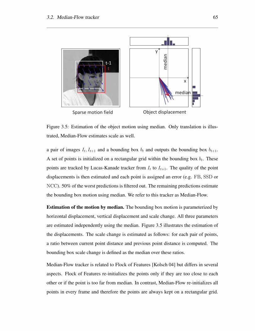
3.2. Median-Flow tracker 65
t-1t
x
y
me
dia
n
median
Sparse motion field Object displacement
Figure 3.5: Estimation of the object motion using median. Only translation is illus-
trated, Median-Flow estimates scale as well.
a pair of images It, It+1 and a bounding box bt and outputs the bounding box bt+1.
A set of points is initialized on a rectangular grid within the bounding box bt. These
points are tracked by Lucas-Kanade tracker from It to It+1. The quality of the point
displacements is then estimated and each point is assigned an error (e.g. FB, SSD or
NCC). 50% of the worst predictions is filtered out. The remaining predictions estimate
the bounding box motion using median. We refer to this tracker as Median-Flow.
Estimation of the motion by median. The bounding box motion is parameterized by
horizontal displacement, vertical displacement and scale change. All three parameters
are estimated independently using the median. Figure 3.5 illustrates the estimation of
the displacements. The scale change is estimated as follows: for each pair of points,
a ratio between current point distance and previous point distance is computed. The
bounding box scale change is defined as the median over these ratios.
Median-Flow tracker is related to Flock of Features [Kolsch 04] but differs in several
aspects. Flock of Features re-initializes the points only if they are too close to each
other or if the point is too far from median. In contrast, Median-Flow re-initializes all
points in every frame and therefore the points are always kept on a rectangular grid.

66 Chapter 3. Tracking: failure detection
This allows Median-Flow to estimate scale of the object, which is by the Flock of
Features not done. Moreover, Flock of Features requires color and has been applied to
tracking of hands only.
Median-Flow re-initializes the point locations in every frame. This restricts the er-
ror measures that estimate the reliability of the points. In particular, the Forward-
Backward error can consider only a pair of frames, which corresponds to k = 1.
Larger k can not be applied as there are no point trajectories with length k > 1.
3.2.1 Quantitative evaluation
A number of variants of the Median-Flow (MF) tracker were tested. The baseline
tracker MF0 estimates the bounding box displacement based on all points on the
grid. Trackers MFFB,MFNCC,MFSSD estimate the point reliability using FB, NCC
and SSD, respectively. FB performs one backward prediction, NCC and SSD com-
pare consecutive point-centered patches. 50% of the worst points are filtered out.
Tracker MFFB+NCC combines FB and NCC, each error measure independently fil-
ters out 50% of the worst points. These trackers were compared with the following
approaches: Incremental Visual Tracking (IVT) [Ross 07], Online Discriminative Fea-
tures (ODF) [Collins 05], Ensemble Tracking (ET) [Avidan 07] and Multiple Instance
Learning (MIL) [Babenko 09]. The evaluation was performed on 6 video sequences
from [Yu 08]. The sequences contain appearance changes, fast motion, and partial
occlusion and in some cases the object disappears from the camera view and later
reappears. The sequences are described in detail in Appendix B.
Evaluation protocol. The objects were manually initialized in the first frame and
tracked up to the end of the sequence. The trajectory was considered correct if the
bounding box overlap with ground truth was larger than 50%. The overlap was defined
as a ratio between intersection and union of two bounding boxes. Performance was
assessed as the maximal frame number up to which the tracker was correct.

3.2. Median-Flow tracker 67
Sequence Frames IVT ODF ET MIL MF0 MFFB MFNCC MFSSD MFFB+NCC
[Ross 07] [Collins 05] [Avidan 07] [Babenko 09]
David 761 17 n/a 94 135 93 761 144 28 761
Jumping 313 75 313 44 313 36 76 87 79 170
Pedestrian 1 140 11 6 22 101 15 37 40 12 140
Pedestrian 2 338 33 8 118 37 97 97 97 97 97
Pedestrian 3 184 50 5 53 49 52 52 52 52 52
Car 945 163 n/a 10 45 248 510 394 353 510
Best n/a 0 1 2 1 0 2 0 0 3
Table 3.1: Comparison of the Median-Flow tracker with state-of-the-art approaches in
terms of the number of correctly tracked frames.
0
1
frame number, length 140
tracker
overlap w
ith g
round tru
th
all
FB
NCC
SSD
FB+NCC
Figure 3.6: Comparison of various variants of the Median-Flow tracker.
Table 3.1 shows the quantitative results for all sequences. The last row shows the num-
ber of times the particular algorithm performed best. The best results were obtained
by the Median-Flow based on a combination of FB and NCC error. This tracker was
able to score best three times.
Figure 3.6 shows the bounding box overlap with the ground truth as a function of time
for several variants of the Median-Flow tracker. The baseline T0 tracker as well as
TSSD loose the object quickly after initialization (overlap goes to zero). TFB and TNCC
perform better and are able to follow the object for twice as long than the baseline
method. TFB+NCC dominates and is able to track the target throughout entire sequence.
This result shows partial complementarity of FB and NCC.
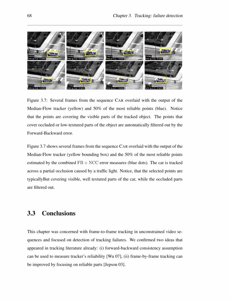
68 Chapter 3. Tracking: failure detection
Figure 3.7: Several frames from the sequence CAR overlaid with the output of the
Median-Flow tracker (yellow) and 50% of the most reliable points (blue). Notice
that the points are covering the visible parts of the tracked object. The points that
cover occluded or low-textured parts of the object are automatically filtered out by the
Forward-Backward error.
Figure 3.7 shows several frames from the sequence CAR overlaid with the output of the
Median-Flow tracker (yellow bounding box) and the 50% of the most reliable points
estimated by the combined FB + NCC error measures (blue dots). The car is tracked
across a partial occlusion caused by a traffic light. Notice, that the selected points are
typicallyBut covering visible, well textured parts of the car, while the occluded parts
are filtered out.
3.3 Conclusions
This chapter was concerned with frame-to-frame tracking in unconstrained video se-
quences and focused on detection of tracking failures. We confirmed two ideas that
appeared in tracking literature already: (i) forward-backward consistency assumption
can be used to measure tracker’s reliability [Wu 07], (ii) frame-by-frame tracking can
be improved by focusing on reliable parts [Jepson 03].

3.3. Conclusions 69
First, we proposed a novel measure, Forward-Backward error, which evaluates relia-
bility of arbitrarily long trajectories. The benefits of the measure and complementar-
ity to appearance-based SSD were shown. Second, we developed a novel frame-to-
frame tracker, Median-Flow, which internally estimate reliability of its components.
We showed that the Median-Flow works best when the reliability is estimated using
combined FB and NCC errors. Superior performance in comparison to state-of-the-
art trackers was demonstrated on several sequences.
Like any other frame-to-frame tracker, Median-Flow eventually fails. This is appar-
ent in table 3.1 (sequences JUMPING, PEDESTRIAN 2 and PEDESTRIAN 3) where all
tested trackers failed due to full occlusion or disappearance of the tracked object. This
shows that the frame-to-frame tracking has its limitations and a different model has
to be developed in order to handle such sequences. In particular, detection based ap-
proaches consider every frame as independent and therefore can handle full occlusions.
This approach will be investigated in the following chapter.

70 Chapter 3. Tracking: failure detection

Chapter 4
Detection: supervised bootstrap
This chapter investigates long-term tracking from the perspective of object detection.
For a large number of tracking scenarios, the visual class of the object of interest is
known. It is therefore possible to train an object class detector in advance and integrate
it into the tracking process. This approach has been successfully applied to a variety
of scenarios including tracking of human faces [Li 07], pedestrians [Leibe 07] or ice-
hockey players [Okuma 04]. If the information about the object class is available, a
long-term tracker should be able to use it. Therefore, our goal is to develop a method
for offline learning of object class detectors.
The chapter is organized as follows. In section 4.1 we introduce the problem of large-
scale learning of object detectors. Section 4.2 reviews the related work with the fo-
cus on two most popular training approaches: boosting [Freund 97] and bootstrap-
ping [Sung 98]. Section 4.3 develops a novel learning method that integrates boosting
and bootstrapping optimally. A number of experiments show the properties of the
learning method. Section 4.4 applies the learning method to the training of a face
detector and state-of-the-art performance is achieved. The chapter is concluded in sec-
tion 4.5.
71
72 Chapter 4. Detection: supervised bootstrap
4.1 Introduction
Consider a class of detectors that are based on a scanning window and binary classifi-
cation of image patches [Viola 01]. The crucial problem of these detectors is to train
the binary classifier that covers all appearances of the object and discriminates from
arbitrary background clutter. Efficient processing of large data sets that cover all the
variations is an important problem.
With the information available on the Internet, it is possible to acquire pools of training
data of virtually unlimited sizes. Large pools sideline the problems related to classifier
generalization [Vapnik 98]. Hoverer, due to computational limitations and training
complexity, it is rarely the case that the entire pool can be processed at once. As we
have reviewed in sub-section 2.3.1, one possible solution is to use bootstrapping and
train the classifier iteratively using an active set that focuses on the decision boundary
only. In object detection, bootstrapping is often combined with boosting [Viola 01,
Fleuret 08]. The combination is, however, often ad hoc [Sochman 05], which presents
scope for improvements.
Contributions. The main contribution this chapter is the optimal integration of boot-
strapping with boosting, where the bootstrapping is formalized as a weighted sampling
strategy. We build on the weighted sampling approach [Fleuret 08] and propose a gen-
eralized strategy based on Quasi-random Weighted Sampling + Trimming (QWS+)
that optimally combines its components in order to minimize the variance of hypoth-
esis error in each round of boosting. The QWS+ sampling method is applied to face
detection and leads to a significant increase in the classification performance as well
as the training efficiency on large pools of data.
4.2. Related work 73
4.2 Related work
In object detection, bootstrapping has been used to train a Gaussian mixture model
[Sung 98]. In every round of training, the active set was extended by examples misclas-
sified in previous round and the entire classifier was retrained. The same approach was
applied to refine the decision surface of an SVM classifier [Papageorgiou 98, Dalal 05],
to train the neural network [Rowley 98], or to estimate the histograms of Wavelet co-
efficients [Schneiderman 04].
Viola and Jones [Viola 01] proposed a cascaded classifier composed of a sequence of
stages. A bootstrapping strategy based on re-sampling of the undecided parts of the
pool was used. Many authors followed this approach [Levi 04, Jones 03, Laptev 06].
A number of improvements have been proposed for the classical Viola-Jones cascade.
For example, the standard cascade ignores the confidence which is output from each
stage thus making the classifier unnecessarily long. This drawback was addressed
in [Sochman 05, Wu 04, Xiao 03] where bootstrapping based on (random) re-sampling
and re-weighting of the selected samples according to the confidence was used. Later
on, Fleuret and Geman [Fleuret 08] proposed weighted sampling. Instead of weighting
examples in the active set, examples were sampled with replacement from the pool
with respect to their weights. The approach let to improved classifier performance.
In machine learning literature, Friedman et al. [Friedman 00] proposed trimming, a
technique that selects only a fraction of examples with the highest weights resulting in
an improvement in training speed.
4.3 Integration of bootstrapping and boosting
This section formalizes the combination of boosting and bootstrapping. The analysis
will be performed on AdaBoost formulated as a logistic regression [Friedman 00], but
the proposed method is applicable to other boosting methods as well. The bootstrap-
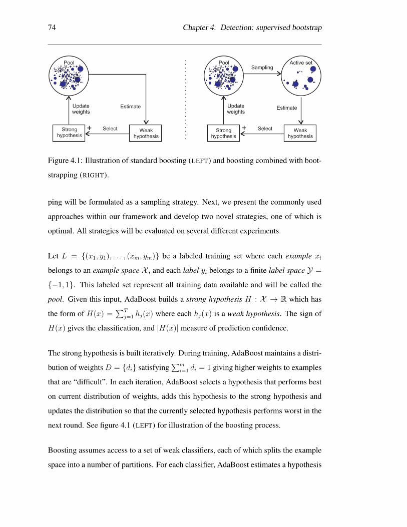
74 Chapter 4. Detection: supervised bootstrap
Active set
Select
Updateweights
Pool
Estimate
Sampling
SelectStronghypothesis
Updateweights
Pool
Estimate
Weakhypothesis
Stronghypothesis
Weakhypothesis
++
Figure 4.1: Illustration of standard boosting (LEFT) and boosting combined with boot-
strapping (RIGHT).
ping will be formulated as a sampling strategy. Next, we present the commonly used
approaches within our framework and develop two novel strategies, one of which is
optimal. All strategies will be evaluated on several different experiments.
Let L = {(x1, y1), . . . , (xm, ym)} be a labeled training set where each example xi
belongs to an example space X , and each label yi belongs to a finite label space Y =
{−1, 1}. This labeled set represent all training data available and will be called the
pool. Given this input, AdaBoost builds a strong hypothesis H : X → R which has
the form of H(x) =∑T
j=1 hj(x) where each hj(x) is a weak hypothesis. The sign of
H(x) gives the classification, and |H(x)| measure of prediction confidence.
The strong hypothesis is built iteratively. During training, AdaBoost maintains a distri-
bution of weights D = {di} satisfying∑m
i=1 di = 1 giving higher weights to examples
that are “difficult”. In each iteration, AdaBoost selects a hypothesis that performs best
on current distribution of weights, adds this hypothesis to the strong hypothesis and
updates the distribution so that the currently selected hypothesis performs worst in the
next round. See figure 4.1 (LEFT) for illustration of the boosting process.
Boosting assumes access to a set of weak classifiers, each of which splits the example
space into a number of partitions. For each classifier, AdaBoost estimates a hypothesis

4.3. Integration of bootstrapping and boosting 75
of the form
h(x) =1
2log
PD(y = 1|x)
1−PD(y = 1|x), (4.1)
where PD(y = 1|x) is a probability estimated using current distribution of weights di.
Boosting then selects the optimal hypothesis h∗ that minimizes
h∗ = arg minh
ZD(h) = arg minh
m∑i=1
die−yih(xi), (4.2)
where ZD(h) is the exponential loss function. Once such a hypothesis is selected,
AdaBoost updates the weights using di ← die−yih∗(xi) and normalizes them to a distri-
bution.
Bootstrapping as a sampling strategy
Standard AdaBoost is not designed for large pools, and therefore, if m is large, the
steps 4.1 and 4.2 may be too time consuming or even not feasible. Therefore, some
form of approximation is needed. Bootstrapping is a process that approximates the
pool of size m by an active set of size n, where n � m. The hypothesis estimation
as well as the selection of the best hypothesis is then performed considering the active
set only. The crucial question is how to approximate the pool correctly. We address
this question by introducing the so-called sampling strategy, which is a process that
takes the distribution of weights D of size m and approximates it by a distribution D
where at most n elements have non-zero value. The approximated distribution must
satisfy∑m
i=1 di = 1. Notice that in general, di 6= di since both of these weights have
to sum-up to one.
Every realization of the sampling strategy results in a different distribution D and thus
different weights di. It follows that di is a random variable with expectation E[di] and
variance Var[di]. If E[di] = di we consider the estimated weights unbiased. Suppose
we have a hypothesis h with a corresponding exponential loss of ZD(h) on distribution
D. When bootstrap is employed, this value is estimated on the active set D according
to the following equation:

76 Chapter 4. Detection: supervised bootstrap
sampling
error
Dis
trib
utio
no
f err
ors
me
asu
red
on
the
active
se
t. Average erroron the active set.
...
PoolActive sets
bias
Error measuredon the pool.
variance
Figure 4.2: Illustration of bias and variance of a bootstrapping strategy.
ZD(h) =m∑i=1
die−yih(xi) (4.3)
where the estimated weights are linearly combined by the constant coefficients e−yih(xi).
Therefore, if the estimated weights di are unbiased then the estimated exponential
loss is unbiased as well. If E[ZD(h)] = ZD(h) then the entire strategy is unbiased.
Var[ZD(h)] will be referred to as a variance of error estimate. The terms bias and
variance are illustrated in figure 4.2.
Conditions for the optimal sampling strategy. Our objective is to find the sampling
strategy that selects n unique samples out of the pool of size m, is unbiased and with
minimal variance of error estimate. Such strategy would guarantee that the approxi-
mate hypothesis h is as close as possible to the optimal one h∗, which would be trained
on the entire pool.
4.3.1 Known sampling strategies
Several bootstrapping strategies have been used in the context of object detection. Here
we formalize the most popular approaches within our notation.

4.3. Integration of bootstrapping and boosting 77
Trimming (Tr). This technique selects n samples from the pool with the highest
weights. The weights of the selected samples are then normalized so that∑
i di = 1.
This strategy was introduced in [Friedman 00], where n was set so that a predefined
fraction (90− 99%) of the total weight mass was used for training. If n < m then the
weights are biased E[di] 6= di with zero variance.
Unique Uniform Sampling (UUS). This strategy selects n unique samples from the
pool with a probability of selecting sample i equal to P(i) = 1m
. The weights of the
selected samples are then normalized so that∑
i di = 1. The estimated weights are
in general biased (due to normalization) and have high variance since it is likely to
disregard examples that carry significant mass of the distribution. Despite this it is
often used in practice [Sochman 05, Wu 04, Xiao 03].
Weighted Sampling (WS). Selects n samples with replacement from the pool. Sam-
ple i is selected with probability P(i) = di and assigned weight di = 1n
. WS is un-
biased, since E[di] = Ndin
= di. Possible implementation: the example weights are
represented as intervals arranged on a unit line segment. Next we generate n random
points on this line segments the positions of which determine the index of the selected
sample. Since the example weight are approximated by repeated selection of the sam-
ple, this strategy does not guarantee n unique samples in the active set. This strategy
was first used in the context of boosting in [Fleuret 08].
4.3.2 Proposed sampling strategies
In this section, we propose new sampling strategies based on WS. These strategies
are designed to reduce the variance of error estimate by quasi-random sampling and
guarantee selection of n unique samples in the active set.

78 Chapter 4. Detection: supervised bootstrap
Quasi-random Weighted Sampling (QWS). QWS reduces variance of the error
estimate by pseudo-random sampling [Press 92]. The weights are represented as in-
tervals and arranged to a unit line segment. The line segment is split into n equal
intervals. Within each interval, one random number is generated, the position of which
determines the index of the selected sample. This process maintains the weights unbi-
ased but significantly reduces their variance. Intuitively, each sample can be selected at
most p-times, where p is number of intervals the sample is covering. For standard WS,
each sample can be selected at most n-times. Since p� n, QWS significantly reduces
the variance of the estimated weights. However, QWS selects an unknown number of
unique samples, which may lead to ineficient usage of available memory.
Quasi-random Weighted Sampling + Trimming (QWS+). The QWS+ is a gen-
eralization of Trimming and QWS, parameterized by k, the number of samples with
largest weights in the pool that are always selected (trimmed). For k = n, QWS+
coincides with trimming. For k = 0, QWS+ becomes a QWS. For any 0 ≤ k < n,
the QWS+ strategy is unbiased, since weighted sampling is unbiased and calculations
of exponential loss on the trimmed set is exact. Parameter k is set to minimize the
variance of the error estimate.
Intuitively, QWS+ selects k most dominant samples that would be selected by QWS
with probability at least 50% and assigns them their own weights. The remaining
weight mass is distributed amongst the remaining l = n − k samples selected by
QWS. Trimming of the most dominant samples reduces the variance of their estimated
weight and hence the variance of the entire distribution.
In the following theorem, we show the optimal setting of the parameter k. We use
the following notation. Index in parenthesis denotes sample with (i)-th largest weight.
S = {X,D} represents the pool augmented with the distribution of weights that shall
be called the weighted pool. Sk is the weighted pool without k samples with largest
weights, Dk = 1 −∑k
i=1 d(i) is the weight mass of Sk, and ZQWS+(S, h) is the ex-

4.3. Integration of bootstrapping and boosting 79
ponential loss of hypothesis h on weighted pool S when approximated by sampling
strategy QWS+.
Theorem: The optimal size of trimming is the largest k that satisfies the condition1l≤ d(k)
Dk(2 +
d(k)Dk
), if variance of exponential loss of h changes ”slowly” (defined
below).
Proof: First, we express the exponential loss of QWS+ strategy as two components
(trimming and weighted sampling) parameterized by k:
ZQWS+(S, h) =k∑i=1
d(i)e−y(i)h(x(i)) + ZQWS(Sk, h) (4.4)
≈k∑i=1
d(i)e−y(i)h(x(i)) + ZWS(Sk, h). (4.5)
We assume that ZQWS(Sk, h) ≈ ZWS(Sk, h) which results in simplified analysis. The
difference between sampling with and without replacement is in this case small since
all k dominant samples were already removed by trimming.
Weighted sampling selects l = n − k samples with replacement from Sk. Sample i
is selected with probability P (i) = diDk
and assigned weight di = Dkl
. The random
variable ZWS is thus a re-scaled sum of l random variables corresponding to each
sample:
ZWS =Dk
l
l∑s=1
ZsWS, (4.6)
where random variables ZsWS attain the value e−yi(s)h(xi(s)) with probability di(s)
Dk, i(s) is
the index chosen in step s.
Next, we express the variance of the exponential loss. From equation 4.5 we can see
that variance of ZQWS+ can be approximated by the variance of ZWS since a trimming

80 Chapter 4. Detection: supervised bootstrap
has variance equal to zero. Variance of ZWS is further substituted from equation 4.6
yielding the form:
Var[ZQWS+] ≈ Var[ZWS] = Var[Dk
l
l∑s=1
ZsWS] =
D2k
l
l∑s=1
Var[ZsWS]. (4.7)
After substituting∑1
s=1 Var[ZsWS] with ck, we obtain a simplified equation
Var[ZQWS+] ≈D2k
lck. (4.8)
Our goal is now to find conditions for k that minimize the variance. We assume that
ck changes slowly as a function of k, i.e. ckck−1≈ 1. For interesting cases, where the
number of training examples is large and the dominant weights are already removed
by trimming, is this condition satisfied. In the following, we express the optimality
condition that variance of exponential loss for k must be smaller than for k − 1:
D2k
lck ≤
D2k−1
l + 1ck−1 =
(Dk + d(k))2
l + 1ck−1 ,
ckck−1
≈ 1
l + 1
l≤
(Dk + d(k))2
D2k
(4.9)
1
l≤
d(k)Dk
(2 +d(k)Dk
) ≈2d(k)Dk
, (4.10)
which concludes the proof. In practice, the optimal k is found iteratively. Samples are
trimmed until the equation 4.10 is satisfied.
4.3.3 Properties of sampling strategies
This sub-section comparatively evaluates the existing and proposed sampling strategies
on synthetic data. In particular, the impact of the sampling strategy on the bias and
variance is investigated.
Estimation of weights. This experiment visualizes the estimation of weights for the
discussed strategies. A pool of size m = 15 with randomly assigned weights di was

4.3. Integration of bootstrapping and boosting 81
Trimming
index
we
igh
ts
UUS
index
WS
index
QWS
index
QWS+
index
Figure 4.3: Pool with weights di (blue bars) is repeatedly sampled to obtain a distri-
bution of the estimated weights. The range of the distribution (1 and 99% quantiles) is
depicted by red vertical lines and expected values by circles.
randomly generated. The active set of size n = 5 was sampled 1000 times, each
realization outputs a set of estimated weights di. For each estimated weight and strat-
egy, the expected value and the variance was computed as shown in figure 4.3. The
circles in the figure denote the expectation of the estimated weight. The variance of
the estimated weights is depicted by the red error bars. Notice that the expectation
of Trimming and UUS is biased, the remaining strategies are not. Note the reduction
of variance by Quasi-random Weighted Sampling strategies (QWS, QWS+). Further-
more, QWS+ completely eliminates variance on large examples which leads to the
minimal variance of all tested strategies.
Estimation of exponential loss of a given hypothesis. In this experiment, we created
a pool containing m = 95, 000 examples with distribution of weights after the 100th
iteration of training a face detector (details later). Using this entire training set, the
optimal hypothesis h∗ was found and its exponential loss ZD(h∗) was measured. The
pool was than sampled by each strategy to obtain 1000 active sets of size n = 500.
Next, the optimal hypothesis was tested on each active set to obtain its approximated
exponential loss ZD(h∗). The expectation and variance of ZD(h∗) is shown in fig-
ure 4.4 (a). Weighted sampling reduces significantly the variance of ZD(h∗) and keeps
mean unbiased. Intuitively, the exponential loss is dominated by examples with high
weights, weighted sampling forces these examples to be included in every realization

82 Chapter 4. Detection: supervised bootstrap
Figure 4.4: The variance and bias of the sampling strategies. The dashed line shows
the exponential loss of the optimal hypothesis. (a) Exponential loss measured of a
given hypotheis, (b) exponential loss measured on training data, (c) exponential loss
measured on testing data. See text for more details.
of the active set, and hence the exponential loss in different trials is similar. Notice that
the variance for QWS and QWS+ is further reduced with respect to WS.
Exponential loss estimated on training and testing data. In this experiment we use
the same sets as defined in the previous paragraph. The optimal hypothesis h∗ was first
trained on full pool and the corresponding exponential loss ZD(h∗) was measured. The
hypothesis was trained by the domain partitioning approach [Schapire 99]. Next, for
each strategy and realization of an active set, we trained an approximate hypothesis h.
We estimated the training exponential loss ZD(h) and testing exponential loss ZD(h).
Figure 4.4 (b, c) shows the mean and variance of the training and testing exponential
loss. Note, that UUS sampling overfits the training data more than any of the other
strategies, i.e. training loss is lower and testing loss is higher than the optimal loss
value. Furthermore, the variance of UUS is the highest of all the strategies. The
variance is significantly reduced for WS. QWS and QWS+ further reduce the variance,
but the difference with respect to WS is subtle. This apparently insignificant difference
in the variance reduction proves to be of importance, when full detector training is
evaluated.

4.4. Application to face detection 83
Face database Details
Frontal (LFRONT) 3 085 frontal faces collected from www.betaface.com,
annotated by a 3rd party face detector + manual check.
Profile (LβPROF) 3 384 manually annotated profile faces from 8 movies,
β indicates in-plane rotation.
Background (LNONE) 3 310 images that were manually checked to contain no faces.
Table 4.1: Data sets used for training of a face detector.
4.4 Application to face detection
This section applies the proposed learning method to training of several face detectors
(frontal, profile, specific). We build on WaldBoost [Sochman 05] algorithm, which
uses a UUS strategy and extended it with the proposed sampling strategies.
Training details. We have collected three training sets shown in table 4.4 which
contain frontal, profile and multi-view faces as well as images depicting background.
The training sets consist of tightly cropped face-patches of size 28 × 28 pixels. The
patches are described using three types of features: (i) Haar-like wavelets [Jones 03],
(ii) Local Binary Patterns (LBP) [Ojala 02], and (iii) Histogram of Orientated Gradi-
ents (HOG) [Dalal 05] projected into one dimension using weighted Linear Discrim-
inant Analysis [Laptev 06]. We generate a feature set of approximately 12 000 Haar,
12 000 LBP and 400 HOG features differing in their localization within the patch, scale
and aspect ratio. The resulting detectors are tested on standard CMU-MIT1 data sets
and compared with other approaches using Receiving Operating Characteristic (ROC)
and Precision and Recall Curves (PRC).
1http://vasc.ri.cmu.edu/idb/html/face/

84 Chapter 4. Detection: supervised bootstrap
0 0.5 10
0.2
0.4
0.6
0.8
1
recall
pre
cis
on
N = 100
0 0.5 10
0.2
0.4
0.6
0.8
1
recall
pre
cis
on
N = 10000
0 0.5 10
0.2
0.4
0.6
0.8
1
recallp
recis
on
N = 1000
UUSWSQWSQWS+
Figure 4.5: The detector performance as a function of the active set size and the sam-
pling strategy. The pool consists of 10 000 positive and 56 million negative examples.
4.4.1 Frontal face detector
This experiment trains a frontal face detector and investigates the influence of rela-
tive active set size on the detector performance. We used the pool of 10 000 positive
examples and 56 million background patches. The positive examples were generated
from LFRONT using shift and in-plane rotation of the original face-patches. The negative
patches were sampled from LNONE using a sliding window. This pool was approxi-
mated by active sets of three different sizes n ∈ {100, 1 000, 10 000}. For each size
and sampling strategy (UUS, WS, QWS, QWS+), a strong classifier was trained up to
the length of 200 features. Trimming was also tested but its performance was much
worse than any other strategy.
Figure 4.5 shows the resulting PRC curves on the CMU-MIT data set. The perfor-
mance of all sampling strategies decreases with smaller active set size. For large active
sets (n = 10 000) there is almost no difference in performance between the strategies.
For smaller active sets (n = 1 000) the UUS sampling performs significantly worse
than the others. WS is in this case slightly worse than QWS and QWS+. For extremely
small active sets (n = 100) the difference increases. This clearly demonstrates the
benefit of QWS and QWS+. The difference between QWS and QWS+ is in this case

4.4. Application to face detection 85
Falsenegatives
Truenegatives
Truepositives
Falsepositives
Falsepositives
Truenegatives
Truepositives
Falsenegatives
QWS+UUS
Figure 4.6: Performance evaluation: (LEFT) ROC curves on CMU-MIT profile
database (368 profile faces in 208 images). (RIGHT) PRC for specific face detector
applied on the results of Google face search.
on a noise level only. The active set size has impact on training efficiency. While train-
ing with n = 10.000 takes 3 hours, training with n = 100 requires 1 hour on the same
machine.
This experiment demonstrates that the sampling strategy does not play a crucial role in
the case of relatively large active sets, but a significant difference in performance can
be achieved when the active set is relatively small with respect to the pool. QWS and
QWS+ significantly outperformed UUS and WS in that case.
4.4.2 Profile face detector
This experiment trains a profile face detector and compares it with state-of-the-art ap-
proaches. The pool of 41 000 positive and 424 million negative patches was generated
from L0PROF, L15
PROF, L30PROF and LNONE. Two left-profile detectors of length 2 000 were
trained with QWS+ and UUS strategy. The right profile detectors were obtained by
left-to-right flipping of the model.
The resulting ROC curves are displayed in the left panel of figure 4.6. QWS+ has a
86 Chapter 4. Detection: supervised bootstrap
detection rate 5% higher than UUS for 100 false positives. On the same level of false
positives, our detector performs better than the results in [Levi 04] and [Jones 03] and
slightly worse than [Schneiderman 04]. The average number of evaluated weak clas-
sifiers is 5.6 for QWS+ and 7.2 for UUS which shows positive influence of weighted
sampling on the classifier speed. Figure 4.7 illustrate the performance of the profile
face on several images from CMU/MIT data set.
4.4.3 Specific face detector
Google face search was used to collect 650 images returned for query “Borat”2. This
set contained 350 true positives (images depicting Borat), and 300 false positives (im-
ages containing other faces or background). This set was randomly split into training
set and testing set. Using the training set, a specific face detector was trained. The
resulting PRC is presented in the right panel of figure 4.6. Notice that also in this task
the performance of QWS+ is superior to UUS. The specific face detector successfully
finds approximately 80% of faces of Borat with 90% precision.
4.5 Conclusions
We developed an algorithm for training of object detectors from large labeled data sets
and integrated boosting and boosting in a unified algorithm.
Two improvements of standard weighted sampling (WS) are introduced. We designed
quasi-random weighted sampling (QWS) which reduces the variance of error estimate
but does not guarantee unique samples. Next, we introduced a new strategy based on
quasi-random weighted sampling + trimming (QWS+) which removes this drawback.
We provided the theoretical proof of the variance minimization of QWS+.
2A fictional character portrayed by a British comedian Sasha Barron Cohen.

4.5. Conclusions 87
Figure 4.7: Results achieved by our face detector. Bottom row shows the most chal-
lenging faces. The binary executable is available at the website of the author.
The performance of the learning method was demonstrated on the task of generic face
detection. Various characteristics of the learning process were improved: reduction
of the active set; better precision/recall curves and speed. The developed face detec-
tor operates in real-time on QVGA images 3 and therefore is applicable to tracking
scenarios. This detector will be used in chapter 6 for long-term tracking of faces.
We trained a specific face detector from manually checked images returned by Google
face search. This shows that training a specific face detector is feasible, however, the
need of manual preparation of the training set is not practical for long-term tracking
scenarios. In long-term tracking, the training of the specific detector has to be done
online and from unlabeled data.
3Intel Core 2 Duo, 2.40GHz, 2GB RAM

88 Chapter 4. Detection: supervised bootstrap

Chapter 5
Learning: unsupervised bootstrap
This chapter investigates long-term tracking from the perspective of machine learning,
the third component of our system. In particular, we study how to improve an offline
trained object detector during tracking. Our goal is to design a learning approach that
would be suitable for such a scenario as well as general enough to be applicable to
other learning problems.
The chapter is structured as follows. Section 5.1 introduces the problem as online
learning from labeled and unlabeled data. Section 5.2 develops a novel learning paradigm
that we call P-N learning. Section 5.3 applies the P-N learning to training an object de-
tector from a single example and a video stream. The proposed algorithm is evaluated
on a number of challenging sequences. The chapter is concluded in section 5.4.
5.1 Introduction
Consider an object detector and a video stream. The object detector is trained offline
from a limited number of labeled examples and the video stream is unconstrained. The
goal of this chapter is to improve the offline detector by online processing of the video
stream. At every time instance, we run the detector on the current frame, estimate its
89

90 Chapter 5. Learning: unsupervised bootstrap
errors and update the detector so that it does not make such errors in the future. We
refer to this process as unsupervised bootstrap.
The ability to improve an object detector by online processing of an unlabeled video
stream has a large number of applications. Our motivation is long-term tracking where
the online learned detector can be used to re-initialize a frame-to-frame tracker after
its failure. This aspect is studied in chapter 6.
There are several challenges that have to be tackled in order to enable the unsupervised
bootstrap: (i) large variability – the learning must deal with arbitrarily complex video
streams where the object significantly changes appearance, moves in and out of the
camera view, the stream contains background clutter, fast camera motions or motion
blur; (ii) real-time performance – every learning step has to be done immediately after
accepting a new frame; (iii) robustness – the learning should never degrade the classi-
fier, if the video stream does not contain relevant information, the detector performance
should not degrade.
To tackle all these challenges, we rely on the various information sources contained
in the video. Consider, for instance, a single patch denoting the object location in a
single frame. This patch defines not only the appearance of the object, but also deter-
mines the surrounding patches, which define the appearance of the background. When
tracking the patch, one can discover different appearances of the same object as well as
more appearances of the background. This is in contrast to standard machine learning
approaches, where the training examples are considered to be independent [Blum 98].
This opens interesting questions how to effectively exploit the information in the video
during learning.
To exploit the information in the video, we propose a new learning paradigm called P-N
learning. The detector is evaluated on every frame of the video stream with the aim to
find misclassified examples. These misclassified examples are estimated by two types
of complementary ”experts”: (i) P-expert – an expert on positive examples, estimates
when the object detector missed the object, and (ii) N-expert – an expert on negative
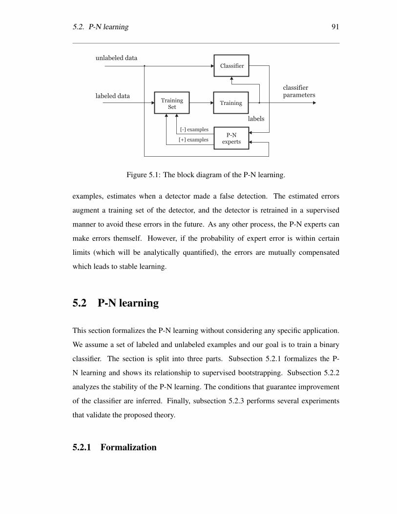
5.2. P-N learning 91
Training
P-Nexperts
Classifier
unlabeled data
TrainingSet
labeled data
labels
classifierparameters
[+] examples
[-] examples
Figure 5.1: The block diagram of the P-N learning.
examples, estimates when a detector made a false detection. The estimated errors
augment a training set of the detector, and the detector is retrained in a supervised
manner to avoid these errors in the future. As any other process, the P-N experts can
make errors themself. However, if the probability of expert error is within certain
limits (which will be analytically quantified), the errors are mutually compensated
which leads to stable learning.
5.2 P-N learning
This section formalizes the P-N learning without considering any specific application.
We assume a set of labeled and unlabeled examples and our goal is to train a binary
classifier. The section is split into three parts. Subsection 5.2.1 formalizes the P-
N learning and shows its relationship to supervised bootstrapping. Subsection 5.2.2
analyzes the stability of the P-N learning. The conditions that guarantee improvement
of the classifier are inferred. Finally, subsection 5.2.3 performs several experiments
that validate the proposed theory.
5.2.1 Formalization

92 Chapter 5. Learning: unsupervised bootstrap
Algorithm 1 P-N learningRequire: unlabeled data, labeled data
Require: classifier trained using labeled data
for t = 1 :∞ do
Evaluate current classifier on unlabeled data.
Estimate false negatives using N-expert.
Estimate false positives using P-expert.
Add estimated errors to training set.
Retrain or update the classifier.
end for
Let x be an example from a feature-space X and y be a label from a space of labels
Y = {−1, 1}. A set of examples X is called an unlabeled set, Y is called a set of
labels and L = {(x, y)} is called a labeled set. The input to the P-N learning is a
labeled set Ll and an unlabeled set Xu, where l � u. The task of P-N learning is to
learn a classifier f : X → Y from labeled set Ll and bootstrap its performance by the
unlabeled set Xu. Classifier f is a function from a family F parameterized by Θ. The
family F is subject to implementation and is considered fixed in training, the training
therefore corresponds to estimation of the parameters Θ.
The P-N learning consists of four blocks: (i) classifier to be learned, (ii) training set
– a collection of labeled training examples, (iii) supervised training – a method that
trains a classifier from the training set, and (iv) P-N experts – functions that estimate
errors of the classifier and augment the training set with labeled examples. Figure 5.1
shows a block diagram and algorithm 1 defines a pseudo-code.
The training process is initialized by inserting the labeled examples Ll into the training
set. The training set is then passed to supervised learning which trains a classifier,
i.e. estimates the initial parameters Θ0. The learning process then proceeds iteratively.
In iteration k, the classifier trained in iteration k − 1 classifies the entire unlabeled
set, yku = f(xu|Θk−1) for all xu ∈ Xu. The classification is analyzed by the P-N

5.2. P-N learning 93
experts that estimate, which examples have been classified incorrectly. These examples
are added with changed labels to the training set. The iteration finishes by retraining
the classifier, i.e. estimation of Θk. The process iterates until convergence or other
stopping criterion.
The crucial element of P-N learning is the estimation of the classifier errors. The
key idea is to treat the estimation of false positives independent from estimation of
false negatives. For this reason, the unlabeled set is split into two parts based on the
current classification and each part is analyzed by an independent expert. The P-expert
analyzes examples classified as negative, estimates false negatives and adds them to
the training set with a positive label. In iteration k, P-expert outputs n+(k) positive
examples. N-expert analyzes examples classified as positive, estimates false positives
and adds them with negative label to the training set. In iteration k, the N-expert
outputs n−(k) negative examples. The P-expert influences the classifier in positive
(growing) sense and increases the classifier generality. The N-expert influences the
classifier in a negative (pruning) sense and increases the classifier discriminability.
These two forces are working in parallel and independently from each other.
Relation to supervised bootstrap. To put P-N learning into context, let us consider
that the labels of set Xu are known. Under this assumption it is straightforward to
design P-N experts that identify misclassified examples and add them to the training set
with correct labels. Such a strategy corresponds to a supervised bootstrap as discussed
in chapter 4. A classifier trained using supervised bootstrap focuses on the decision
boundary and often outperforms a classifier trained on a randomly sampled training
set [Sung 98]. The same idea of focusing on the decision boundary underpins the P-N
learning approach with the difference that the labels of the set Xu are unknown. P-
N learning can be therefore viewed as a generalization of standard bootstrapping to
unlabeled cases where labels are not given but rather estimated using the P-N experts.
As any other process, the P-N experts make errors, and estimate the labels incorrectly.
Such errors propagate through the training, which will be now theoretically analyzed.

94 Chapter 5. Learning: unsupervised bootstrap
5.2.2 Stability
This section analyses the impact of the P-N learning on the classifier performance and
the impact of the errors caused by P-N experts on the stability of the learning. For the
purpose of the analysis, let us consider that the ground truth labels of Xu are known
and therefore it is possible to measure the errors made by the classifier. Next, consider
a classifier that initially classifies the unlabeled set at random and then corrects its
classification according to the output of the P-N experts. The performance of such
a classifier is characterized by a number of false positives FP(k) and a number of
false negatives FN(k), where k indicates the iteration of training. The goal of the P-N
learning is to reduce these errors to zero.
In iteration k, the P-expert outputs n+c (k) positive examples which are correct (positive
based on ground truth), and n+f (k) positive examples which are false (negative based on
ground truth), which forces the classifier to change n+(k) = n+c (k)+n+
f (k) negatively
classified examples to positive. Similarly, the N-experts outputs n−c (k) correct negative
examples and n−f (k) false negative examples, which forces the classifier to change
n−(k) = n−c (k) + n−f (k) examples classified as positive to negative. The number
of false positive and false negative errors of the classifier in the next iteration thus
becomes:
FP(k + 1) = FP(k)− n−c (k) + n+f (k) (5.1a)
FN(k + 1) = FN(k)− n+c (k) + n−f (k). (5.1b)
Equation 5.1a shows that false positives FP(k) decrease if n−c (k) > n+f (k), i.e. number
of examples that were correctly relabeled to negative is higher than the number of
examples that were incorrectly relabeled to positive. Similarly, the false negatives
FN(k) decrease if n+c (k) > n−f (k).
Quality measures. In order to analyze the convergence of the P-N learning, a model
needs to be defined that relates the quality of the P-N experts to the absolute number of

5.2. P-N learning 95
positive and negative examples output in each iteration. The quality of the P-N experts
is characterized by four quality measures:
• P-precision – reliability of the positive labels, i.e. the number of correct positive
examples divided by the number of all positive examples output by the P-expert,
P+ = n+c /(n
+c + n+
f ).
• P-recall – percentage of identified false negative errors, i.e. the number of cor-
rect positive examples divided by the number of false negatives made by the
classifier, R+ = n+c /FN.
• N-precision – reliability of negative labels, i.e. the number of correct nega-
tive examples divided by the number positive examples output by the N-expert,
P− = n−c /(n−c + n−f ).
• N-recall – percentage of recognized false positive errors, i.e. the number of
correct negative examples divided by the number of all false positives made by
the classifier, R− = n−c /FP.
Given these quality measures, the number of correct and false examples output by P-N
experts at iteration k have the form:
n+c (k) = R+ FN(k), n+
f (k) =(1− P+)
P+R+ FN(k) (5.2a)
n−c (k) = R− FP(k), n−f (k) =(1− P−)
P−R− FP(k). (5.2b)
By combining the equation 5.1a, 5.1b, 5.2a and 5.2b we obtain:
FP(k + 1) = (1−R−) FP(k) +(1− P+)
P+R+ FN(k) (5.3a)
FN(k + 1) =(1− P−)
P−R− FP(k) + (1−R+) FN(k). (5.3b)
After defining the state vector ~x(k) =[FP(k) FN(k)
]Tand a 2× 2 matrix M as
M =
1−R− (1−P+)P+ R+
(1−P−)P− R− (1−R+)
(5.4)

96 Chapter 5. Learning: unsupervised bootstrap
l1=0, l2< 1
a
b b b
a a
l1=0, l2=1 l1
=0, l2> 1
Figure 5.2: The evolution of errors of the classifier depends on the quality of the P-N
experts, which is defined in terms of eigenvalues of matrix M. The errors converge to
zero (LEFT), are at the edge of stability (MIDDLE) or are growing (RIGHT).
it is possible to rewrite the equations as
~x(k + 1) = M~x(k).
This is a recursive equation that corresponds to a discrete dynamical system. The
system models the error propagation during training, i.e. from one iteration of P-N
learning to another. Our goal is to show, under which conditions the error in the system
drops.
Based on the stability criteria from control theory [Zhou 96, Ogata 09], the state vector
~x converges to zero if both eigenvalues λ1, λ2 of the transition matrix M are smaller
than one. Note that the matrix M is a function of the expert quality measures. There-
fore, if the quality measures are known, it is possible to check whether the error during
training converges to zero or not. Experts for which the corresponding matrix M has
both eigenvalues smaller than one will be called error-canceling. Figure 5.2 illustrates
the evolution of error of the classifier when the first eigenvalue is zero and the second
eigenvalue attains values (i) λ2 < 1, (ii) λ2 = 1, and (iii) λ2 > 1.
The pragmatic reason for developing the P-N learning theory was the observation, that
it is relatively simple to design a large number of experts that correct specific errors

5.2. P-N learning 97
made by the classifier. The combined influence of the experts was, however not under-
stood. P-N learning represents guidelines how to combine a number of weak experts so
that the overall learning is stable. Interestingly, P-N learning does not put constraints
on the quality of individual experts. Even experts with low precision might be used as
long as the matrix M has eigenvalues smaller than one, it is therefore possible to use
various (even weak) information sources.
5.2.3 Experiments
This section analyzes the performance of P-N learning as a function of the expert
quality measures. Our goal is to experimentally validate the claims about learning
stability that have been made in section 5.2.2. The experiment is based on synthetically
generated P-N experts.
Experiment setup. The analysis is performed on sequence CAR (see Appendix B). In
the first frame of the sequence, a classifier is trained using affine warps of the initial
patch and background patches from the surrounding of the object. Details about this
step are given in chapter 7. Next, a single run over the sequence is performed. In
every frame, the classifier is evaluated. The error of the classifier are recognized using
simulated experts that are characterized by chosen quality measures and the classifier
is updated. After every update, the classifier is tested on the entire sequence using
f-measure. The performance is then drawn as a function of the number of processed
frames and the quality of the P-N experts.
The P-N experts are characterized by four quality measures, P+, R+, P−, R−. To
reduce this 4D space of parameters, we analyze the learning at equal error rate. The
parameters are set to P+ = R+ = P− = R− = 1− ε, where ε represents error of the
expert. The transition matrix then becomes M = ε[11]T, where [11]T is a 2x2 matrix
of ones. The eigenvalues of this matrix are λ1 = 0, λ2 = 2ε. Therefore, based on the
theory, the P-N learning should be improving the performance if ε < 0.5.

98 Chapter 5. Learning: unsupervised bootstrap
0 1000
0
1
Number of Frames Processed
F-M
easu
re
0.0
0.5
0.6
Figure 5.3: Performance of a detector as a function of the number of processed frames.
The detectors were trained by synthetic P-N experts with guaranteed level of error. The
classifier is improved up to error 50% (BLACK), higher error degrades it (RED).
The experts were realized using the ground truth data as follows. In frame k the clas-
sifier generates FN(k) false negatives. P-experts relabel n+c (k) = (1 − ε) FN(k) of
them to positive which guarantees R+ = 1 − ε. In order to satisfy the requirement of
precision P+ = 1 − ε, the P-expert relabels additional n+f (k) = εFN(k) background
samples to positive. Therefore the total number of examples relabeled to positive in
iteration k is n+ = n+c (k) + n+
f (k) = FN(k). The N-experts were generated similarly.
The performance of the classifier as a function of number of processed frames is de-
picted in figure 5.3. Notice that if ε ≤ 0.5 the performance of the detector increases
with more processed frames. In theory, ε = 0.5 should not alter the classifier perfor-
mance, although in this sequence it leads to improvements. Increasing the noise-level
further leads to sudden degradation of the classifier.
The P-N learning with error-less experts (ε = 0) is analyzed in more detail. In this
case all classifier errors are identified and no miss-labeled examples are added to the
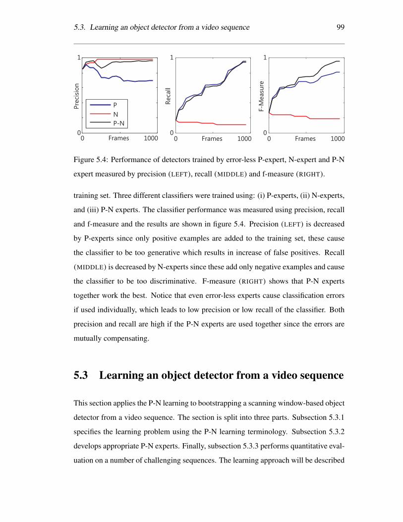
5.3. Learning an object detector from a video sequence 99
0 10000
1
Pre
cis
ion
Frames 0 10000
1
Recall
Frames 0 10000
1
F-M
easu
re
Frames
P
N
P-N
Figure 5.4: Performance of detectors trained by error-less P-expert, N-expert and P-N
expert measured by precision (LEFT), recall (MIDDLE) and f-measure (RIGHT).
training set. Three different classifiers were trained using: (i) P-experts, (ii) N-experts,
and (iii) P-N experts. The classifier performance was measured using precision, recall
and f-measure and the results are shown in figure 5.4. Precision (LEFT) is decreased
by P-experts since only positive examples are added to the training set, these cause
the classifier to be too generative which results in increase of false positives. Recall
(MIDDLE) is decreased by N-experts since these add only negative examples and cause
the classifier to be too discriminative. F-measure (RIGHT) shows that P-N experts
together work the best. Notice that even error-less experts cause classification errors
if used individually, which leads to low precision or low recall of the classifier. Both
precision and recall are high if the P-N experts are used together since the errors are
mutually compensating.
5.3 Learning an object detector from a video sequence
This section applies the P-N learning to bootstrapping a scanning window-based object
detector from a video sequence. The section is split into three parts. Subsection 5.3.1
specifies the learning problem using the P-N learning terminology. Subsection 5.3.2
develops appropriate P-N experts. Finally, subsection 5.3.3 performs quantitative eval-
uation on a number of challenging sequences. The learning approach will be described

100 Chapter 5. Learning: unsupervised bootstrap
, )
VIDEO STREAMEXAMPLE P-N Learning
P-expert
corrects missed detections
)error encourages
.
.
.
.
.
.
.
.
.
.
.
.
.
.
.
DETECTOR
N-expert
corrects false alarms
error encourages
Figure 5.5: Given a single example and a video stream, the goal of P-N learning is to
train an accurate object detector.
without considering implementation details, these are given in chapter 6.
5.3.1 Problem specification
The input to the classifier training is a single bounding box and a video sequence. The
learning is performed by sequential processing of the video sequence in a frame-by-
frame fashion. One iteration of P-N learning corresponds to the processing of one
frame of the sequence. The output of the learning is a binary classifier that separates
appearances of the object from appearances of the background that appeared in the
video sequence. Figure 5.5 illustrates the scenario.
The training examples (both labeled and unlabeled) correspond to image patches.
These image patches are sampled at locations and scales determined by a scanning
grid on which the detector operates. The labeled data Ll are extracted from the first
frame. Patches that are overlapping with the initial bounding box are positive, patches
that are non-overlapping are negative. The unlabeled data Xu are contained in the
remaining video sequence.
The learning is initialized in the first frame by supervised training of the so called
Initial detector. The learning then proceeds by sequential processing of the video
sequence. In every frame, the P-N learning performs the following steps: (i) evaluation
of the detector on the current frame, (ii) estimation of the detector errors using the P-N
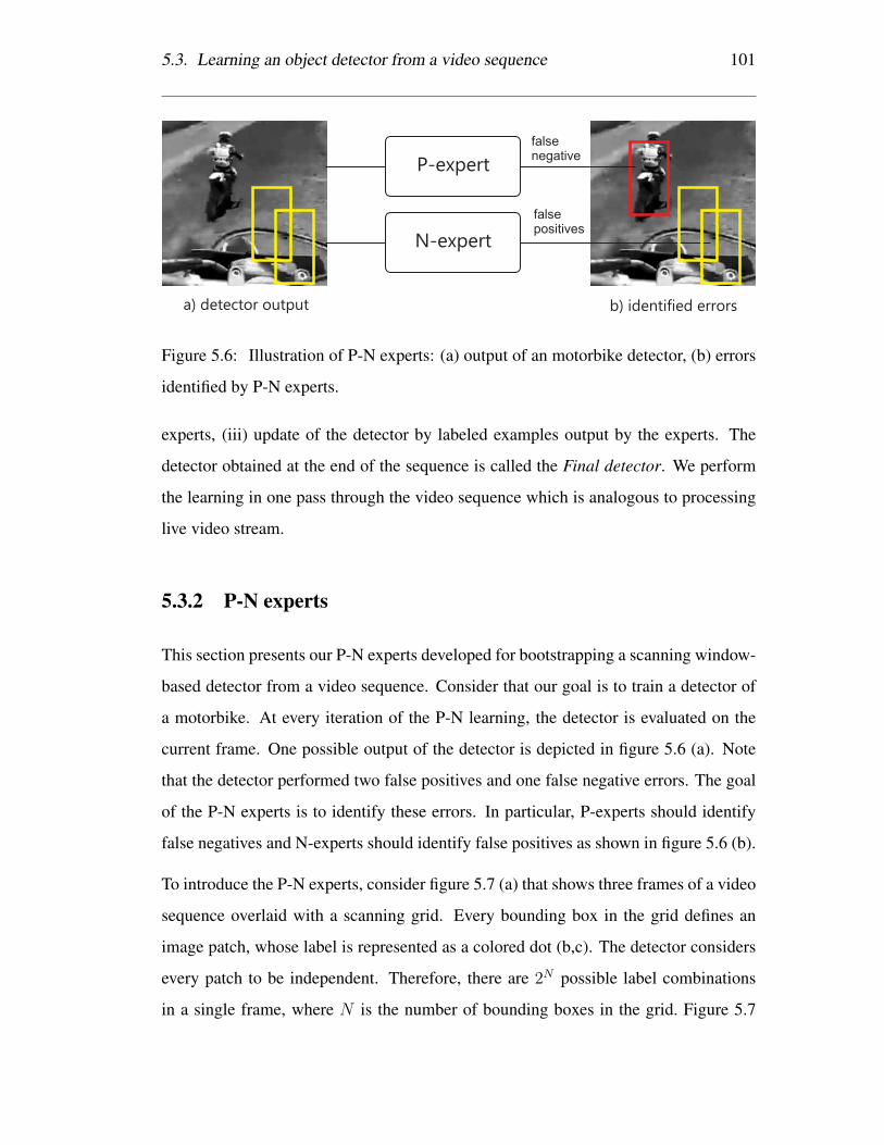
5.3. Learning an object detector from a video sequence 101
falsenegative
falsepositives
a) detector output b) identified errors
P-expert
N-expert
Figure 5.6: Illustration of P-N experts: (a) output of an motorbike detector, (b) errors
identified by P-N experts.
experts, (iii) update of the detector by labeled examples output by the experts. The
detector obtained at the end of the sequence is called the Final detector. We perform
the learning in one pass through the video sequence which is analogous to processing
live video stream.
5.3.2 P-N experts
This section presents our P-N experts developed for bootstrapping a scanning window-
based detector from a video sequence. Consider that our goal is to train a detector of
a motorbike. At every iteration of the P-N learning, the detector is evaluated on the
current frame. One possible output of the detector is depicted in figure 5.6 (a). Note
that the detector performed two false positives and one false negative errors. The goal
of the P-N experts is to identify these errors. In particular, P-experts should identify
false negatives and N-experts should identify false positives as shown in figure 5.6 (b).
To introduce the P-N experts, consider figure 5.7 (a) that shows three frames of a video
sequence overlaid with a scanning grid. Every bounding box in the grid defines an
image patch, whose label is represented as a colored dot (b,c). The detector considers
every patch to be independent. Therefore, there are 2N possible label combinations
in a single frame, where N is the number of bounding boxes in the grid. Figure 5.7

102 Chapter 5. Learning: unsupervised bootstrap
(b) shows one such labeling. The labeling indicates, that the object appears at several
locations in a single frame and there is no temporal continuity in the motion. In natural
videos is such labeling not credible and therefore it can be inferred that the detector
made a mistake at several locations. On the other hand, if the detector outputs classifi-
cation as depicted in (c) the labeling is credible since the object appears at one location
in a single frame and these locations constitute a smooth trajectory in time.
As we have just shown, it is fairly easy to estimate unlikely behavior of the detector
when observing the detector responses in the context of a video volume. We exploited
our prior knowledge about the motion of an object which casts constraints on the la-
beling of the video volume. In other words, every single patch influences labels of
other patches. Such a property will be called structure and the data that has this prop-
erty is structured. This is in contrast to the majority of existing learning algorithms
in semi-supervised learning, which assume that the unlabeled examples are indepen-
dent [Blum 98].
The key idea of the P-N experts is to exploit the structure in the data to estimate the
detector errors. Our approach to modeling the structure is based on simple rules such
as: (i) overlapping patches have the same label, (ii) patches within a single image can
have at most one positive label, (iii) patches that are connected by a trajectory have the
same label, etc. Based on these rules, the P-N experts are built.
The P-expert exploits the temporal structure in the video volume and assumes that
the object moves on a smooth trajectory. The P-expert remembers the location of the
object in the previous frame and estimates the object location in current frame using
a frame-to-frame tracker. If the detector labeled the current location as negative (i.e.
made a false negative error), the P-expert generates a positive example from the current
location and performs an update of the detector.
The N-expert exploits the spatial structure in the video volume and assumes that the
object can appear at a single location in a single frame only. The N-expert analyzes all
responses of the detector in the current frame and the response produced by the tracker
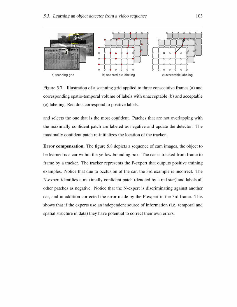
5.3. Learning an object detector from a video sequence 103
a) scanning grid b) not credible labeling c) acceptable labeling
Figure 5.7: Illustration of a scanning grid applied to three consecutive frames (a) and
corresponding spatio-temporal volume of labels with unacceptable (b) and acceptable
(c) labeling. Red dots correspond to positive labels.
and selects the one that is the most confident. Patches that are not overlapping with
the maximally confident patch are labeled as negative and update the detector. The
maximally confident patch re-initializes the location of the tracker.
Error compensation. The figure 5.8 depicts a sequence of cam images, the object to
be learned is a car within the yellow bounding box. The car is tracked from frame to
frame by a tracker. The tracker represents the P-expert that outputs positive training
examples. Notice that due to occlusion of the car, the 3rd example is incorrect. The
N-expert identifies a maximally confident patch (denoted by a red star) and labels all
other patches as negative. Notice that the N-expert is discriminating against another
car, and in addition corrected the error made by the P-expert in the 3rd frame. This
shows that if the experts use an independent source of information (i.e. temporal and
spatial structure in data) they have potential to correct their own errors.

104 Chapter 5. Learning: unsupervised bootstrap
P-expert N-expert
......
*
*
*
Figure 5.8: Illustration of the P-expert and the N-expert and their error compensation.
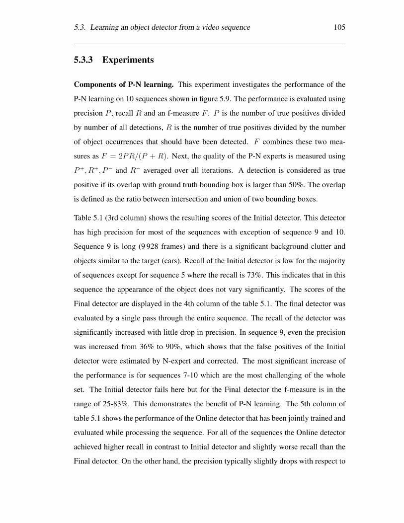
5.3. Learning an object detector from a video sequence 105
5.3.3 Experiments
Components of P-N learning. This experiment investigates the performance of the
P-N learning on 10 sequences shown in figure 5.9. The performance is evaluated using
precision P , recall R and an f-measure F . P is the number of true positives divided
by number of all detections, R is the number of true positives divided by the number
of object occurrences that should have been detected. F combines these two mea-
sures as F = 2PR/(P + R). Next, the quality of the P-N experts is measured using
P+, R+, P− and R− averaged over all iterations. A detection is considered as true
positive if its overlap with ground truth bounding box is larger than 50%. The overlap
is defined as the ratio between intersection and union of two bounding boxes.
Table 5.1 (3rd column) shows the resulting scores of the Initial detector. This detector
has high precision for most of the sequences with exception of sequence 9 and 10.
Sequence 9 is long (9 928 frames) and there is a significant background clutter and
objects similar to the target (cars). Recall of the Initial detector is low for the majority
of sequences except for sequence 5 where the recall is 73%. This indicates that in this
sequence the appearance of the object does not vary significantly. The scores of the
Final detector are displayed in the 4th column of the table 5.1. The final detector was
evaluated by a single pass through the entire sequence. The recall of the detector was
significantly increased with little drop in precision. In sequence 9, even the precision
was increased from 36% to 90%, which shows that the false positives of the Initial
detector were estimated by N-expert and corrected. The most significant increase of
the performance is for sequences 7-10 which are the most challenging of the whole
set. The Initial detector fails here but for the Final detector the f-measure is in the
range of 25-83%. This demonstrates the benefit of P-N learning. The 5th column of
table 5.1 shows the performance of the Online detector that has been jointly trained and
evaluated while processing the sequence. For all of the sequences the Online detector
achieved higher recall in contrast to Initial detector and slightly worse recall than the
Final detector. On the other hand, the precision typically slightly drops with respect to
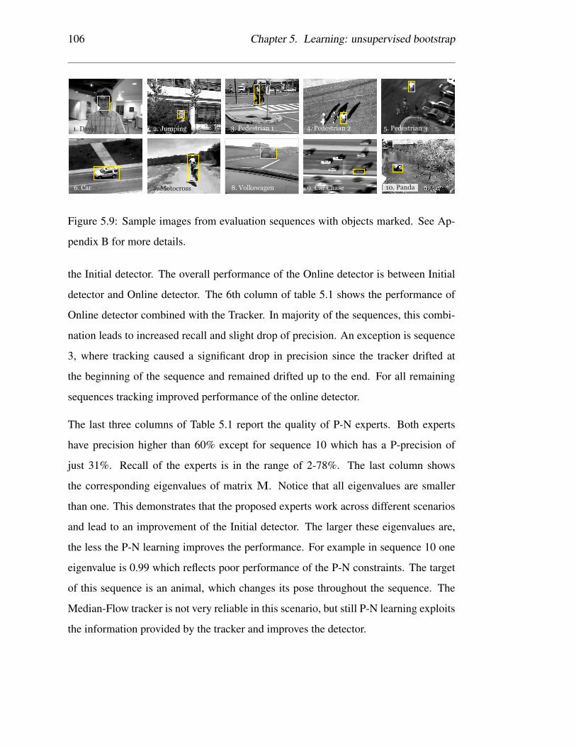
106 Chapter 5. Learning: unsupervised bootstrap
1. David 2. Jumping 3. Pedestrian 1 4. Pedestrian 2 5. Pedestrian 3
6. Car 8. Volkswagen 9. Car Chase 10. Panda7. Motocross
Figure 5.9: Sample images from evaluation sequences with objects marked. See Ap-
pendix B for more details.
the Initial detector. The overall performance of the Online detector is between Initial
detector and Online detector. The 6th column of table 5.1 shows the performance of
Online detector combined with the Tracker. In majority of the sequences, this combi-
nation leads to increased recall and slight drop of precision. An exception is sequence
3, where tracking caused a significant drop in precision since the tracker drifted at
the beginning of the sequence and remained drifted up to the end. For all remaining
sequences tracking improved performance of the online detector.
The last three columns of Table 5.1 report the quality of P-N experts. Both experts
have precision higher than 60% except for sequence 10 which has a P-precision of
just 31%. Recall of the experts is in the range of 2-78%. The last column shows
the corresponding eigenvalues of matrix M. Notice that all eigenvalues are smaller
than one. This demonstrates that the proposed experts work across different scenarios
and lead to an improvement of the Initial detector. The larger these eigenvalues are,
the less the P-N learning improves the performance. For example in sequence 10 one
eigenvalue is 0.99 which reflects poor performance of the P-N constraints. The target
of this sequence is an animal, which changes its pose throughout the sequence. The
Median-Flow tracker is not very reliable in this scenario, but still P-N learning exploits
the information provided by the tracker and improves the detector.

5.3. Learning an object detector from a video sequence 107
Sequence FramesInitial Detector Final Detector Online Detector Online Detector + Tracker P-constraints N-constraints Eigenvalues
Precision / Recall / F-measure Precision / Recall / F-measure Precision / Recall / F-measure Precision / Recall / F-measure P+, R+ P−, R− λ1, λ2
1. David 761 1.00 / 0.01 / 0.02 1.00 / 0.32 / 0.49 0.95 / 0.30 / 0.45 0.94 / 0.94 / 0.94 1.00 / 0.08 0.99 / 0.17 0.92 / 0.83
2. Jumping 313 1.00 / 0.01 / 0.02 0.99 / 0.88 / 0.93 0.89 / 0.60 / 0.72 0.86 / 0.77 / 0.81 0.86 / 0.24 0.98 / 0.30 0.70 / 0.77
3. Pedestrian 1 140 1.00 / 0.01 / 0.02 1.00 / 0.12 / 0.22 1.00 / 0.10 / 0.18 0.22 / 0.16 / 0.18 0.81 / 0.04 1.00 / 0.04 0.96 / 0.96
4. Pedestrian 2 338 1.00 / 0.02 / 0.03 1.00 / 0.34 / 0.51 1.00 / 0.27 / 0.42 1.00 / 0.95 / 0.97 1.00 / 0.25 1.00 / 0.24 0.76 / 0.75
5. Pedestrian 3 184 1.00 / 0.73 / 0.84 0.97 / 0.93 / 0.95 1.00 / 0.85 / 0.92 1.00 / 0.94 / 0.97 0.98 / 0.78 0.98 / 0.68 0.32 / 0.22
6. Car 945 1.00 / 0.04 / 0.08 0.99 / 0.82 / 0.90 1.00 / 0.55 / 0.71 0.93 / 0.83 / 0.88 1.00 / 0.52 1.00 / 0.46 0.48 / 0.54
7. Motocross 2665 1.00 / 0.00 / 0.00 0.92 / 0.32 / 0.47 0.93 / 0.28 / 0.43 0.86 / 0.50 / 0.63 0.96 / 0.19 0.84 / 0.08 0.92 / 0.81
8. Volkswagen 8576 1.00 / 0.00 / 0.00 0.92 / 0.75 / 0.83 0.95 / 0.58 / 0.72 0.67 / 0.79 / 0.72 0.70 / 0.23 0.99 / 0.09 0.91 / 0.77
9. Car Chase 9928 0.36 / 0.00 / 0.00 0.90 / 0.42 / 0.57 0.60 / 0.33 / 0.42 0.81 / 0.43 / 0.56 0.64 / 0.19 0.95 / 0.22 0.76 / 0.83
10. Panda 3000 0.79 / 0.01 / 0.01 0.51 / 0.16 / 0.25 0.71 / 0.09 / 0.16 0.25 / 0.24 / 0.25 0.31 / 0.02 0.96 / 0.19 0.81 / 0.99
Table 5.1: Performance analysis of P-N learning. The Initial detector is trained on the
first frame only. The Final detector is obtained by P-N learning after one pass through
the sequence. The P-N Tracker is the adaptive Lucas-Kanade tracker re-initialized by
the on-line trained detector. The last three columns display internal statistics of the
training process. The statistics were computed for every frame and the table reports
the average values.
Figure 5.10: Several snapshot from face sequence that has been used to evaluate re-
peated runs of P-N learning.
Repeated run over one sequence. This experiment investigates the stability of P-N
learning when run multiple times over a single sequence. We use a benchmark face
sequence that has been first introduced in [Maggio 07]. The sequence contains 1006
frames and shows four face targets in an indoor environment that undergo a variety
of changes including: fast motion, out of plane rotation, partial and full occlusions.
The subject that undergoes the most significant changes was selected for tracking.
Figure 5.10 shows several frames from the sequence.
P-N learning has been run repeatedly on this sequence. After every run, the trained

108 Chapter 5. Learning: unsupervised bootstrap
θL = 0.95 1 2 3 4 5 6 7
Online detector + TrackerPrec 1.00 1.00 1.00 1.00 1.00 1.00 1.00
Rec 0.01 0.01 0.02 0.02 0.03 0.03 0.03
Final DetectorPrec 1.00 1.00 1.00 1.00 1.00 1.00 1.00
Rec 0.00 0.01 0.01 0.01 0.02 0.02 0.02
θL = 0.90
Online detector + TrackerPrec 1.00 1.00 0.99 0.99 0.99 0.95 0.95
Rec 0.04 0.35 0.59 0.68 0.70 0.69 0.71
Final DetectorPrec 1.00 0.99 1.00 0.99 0.99 0.98 0.98
Rec 0.01 0.25 0.49 0.58 0.58 0.61 0.63
θL = 0.80
Online detector +TrackerPrec 1.00 0.97 0.94 0.91 0.91 0.90 0.87
Rec 0.22 0.59 0.70 0.72 0.72 0.71 0.72
Final DetectorPrec 1.00 1.00 0.97 0.93 0.95 0.94 0.89
Rec 0.08 0.46 0.59 0.61 0.65 0.65 0.64
θL = 0.70
Online detector +TrackerPrec 0.98 0.99 0.94 0.94 0.90 0.87 0.87
Rec 0.09 0.57 0.73 0.79 0.78 0.77 0.65
Final DetectorPre 1.00 1.00 0.99 0.97 0.94 0.90 0.93
Rec 0.01 0.35 0.57 0.66 0.68 0.67 0.59
Table 5.2: Performance of P-N learning as a number of runs through the video.
classifier was kept in memory and used as the initial classifier in the next run. The
performance was then accessed using precision and recall as a function of number of
runs over the sequence. We investigated both the performance of the Final detector
as well as the Online detector + Tracker. This experiment was repeated four-times
for different parameter θL which corresponds to rate of learning. The parameter θL is
discussed in chapter 6 section 6.3.6.
The results are presented in table 5.2. Notice the third sub-table with θL = 0.80. In
the first iteration, Online detector + Tracker discovers 22% of the trajectory, while the
Final detector only 8% at the same precision of 100%. With every iteration, the recall
of both of them increases. For θL = 0.95 the learning process does not start at all. The
learning is too conservative in that case. For θL = 0.70 the overall performance first
increases but around 5th iteration it slightly drops and oscillates.

5.4. Conclusions 109
5.4 Conclusions
In P-N learning, a novel approach for the processing of labeled and unlabeled exam-
ples, has been proposed. The underlying assumption of the learning process is that the
unlabeled data are structured. The structure of the data is exploited by positive and
negative experts that restrict the labeling of the unlabeled data. These experts provide
a feedback about the performance of the classifier which is iteratively improved in a
bootstrapping fashion. We have formulated conditions under which the P-N learning
guarantees improvement of the classifier. The conditions have been validated on syn-
thetic and real data. The P-N learning has been applied to the problem of learning of
an object detector from a single example and an unlabeled video sequence. We have
proposed experts that exploit the spatio-temporal properties of a video. These results
open questions such as: (i) under what conditions these experts fail, and (ii) how to
design other experts. These questions are covered chapters 6 and 7.

110 Chapter 5. Learning: unsupervised bootstrap

Chapter 6
Tracking-Learning-Detection (TLD)
This chapter defines, implements and evaluates a new tracking paradigm that we ref-
fer to as Tracking-Learning-Detection (TLD). The chapter is structured as follows.
Section 6.1 introduces the main idea behind TLD. Section 6.2 formalizes the TLD
framework. Section 6.3 describes our implementation. Section 6.4 performs a set of
comparative experiments with state-of-the-art approaches. Section 6.5 applies the TLD
framework to long-term tracking of human faces. Finally, section 6.6 performs a set of
qualitative experiments and discusses the pros and cons.
6.1 Introduction
Consider a video stream and a single bounding box defining the object of interest in
one frame. The goal of long-term tracking is to track the object “forever”: every time,
the object appears in the camera view, a long-term tracker should draw a bounding box
around it. As we have discussed in chapter 2, the long-term tracking problem is closely
related to frame-to-frame tracking and tracking-by-detection.
Frame-to-frame tracking assumes that the object moves on a smooth trajectory. Track-
ers are able to adapt to changes of the object appearance, however, they typically fail if
111

112 Chapter 6. Tracking-Learning-Detection (TLD)
a) Tracker b) Detector c) Tracking-Learning-Detection
x
t
x x
t t
false positives
false negatives
drift failure
occlusion
re-detection
occlusion occlusion
Figure 6.1: Illustration of a tracker (a), detector (b), and a tractor (c). Dotted line shows
ground truth trajectory, gray bar represents full occlusion, thick line is the trajectory of
a tracker, red dots are responses of a detector.
the object gets fully occluded or disappears. In contrast, tracking-by-detection assumes
that the object model is known in advance. The detectors never fail due to occlusion
or disappearance, however, the object model is fixed which means that unexpected
appearances cannot be detected (false positives) and cluttered background may gen-
erate false detections (false positives). Obviously, both of these assumptions are too
restrictive for the long-term tracking problem.
In a number of tracking problems, the objects occasionally reappear with previously
observed appearance. This has been already used to reduce drift of frame-to-frame
tracking [Dowson 05, Rahimi 08], closing loops in SLAM [Newman 06] or tracking of
people [Ramanan 05]. The idea of this chapter is to build online an object detector that
represents all appearances observed so far. This detector shall run in parallel with an
object tracker and correct or re-initalize it when necessary. Tracking is then understood
not only as a way to determine the location of the object, but also as a way to provide
training examples for the online trained object detector. Any algorithm, that combines
an object tracker with an online learned detector will be refered to as tractor. See
figure 6.1 for comparison of a tracker, a detector and a tractor.
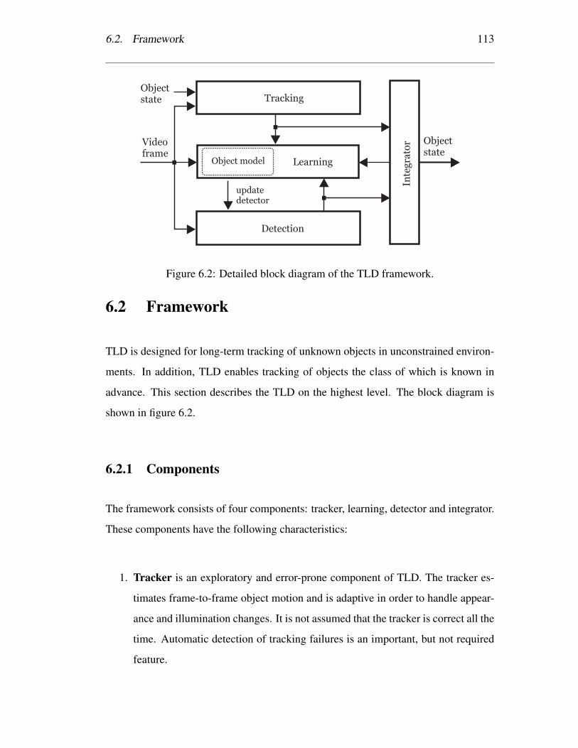
6.2. Framework 113
Tracking
Detection
Inte
gra
tor Object
stateLearning
updatedetector
Videoframe
Object model
Objectstate
Figure 6.2: Detailed block diagram of the TLD framework.
6.2 Framework
TLD is designed for long-term tracking of unknown objects in unconstrained environ-
ments. In addition, TLD enables tracking of objects the class of which is known in
advance. This section describes the TLD on the highest level. The block diagram is
shown in figure 6.2.
6.2.1 Components
The framework consists of four components: tracker, learning, detector and integrator.
These components have the following characteristics:
1. Tracker is an exploratory and error-prone component of TLD. The tracker es-
timates frame-to-frame object motion and is adaptive in order to handle appear-
ance and illumination changes. It is not assumed that the tracker is correct all the
time. Automatic detection of tracking failures is an important, but not required
feature.

114 Chapter 6. Tracking-Learning-Detection (TLD)
2. Learning is an analyzing component that maintains an object model. The object
model. Learning constantly analyzes the output of the tracker and the detector,
estimates errors performed by the detector and updates the object model to avoid
these errors in the future.
3. Detector is a stabilizing component of the system that detect the appearances
represented in the constantly updated object model. The detector is either build
entirely online, or the online information is integrated with prior information
about the object class. The detector must enable efficient incremental update.
4. Integrator is a component that merges the hypotheses from the detector and the
tracker and outputs the final hypothesis about the object state.
TLD distinguishes two modes: (i) initialization, and (ii) run-time.
6.2.2 Initialization
The initialization requires the first frame and the corresponding object state indicated
by a bounding box. In addition, the framework may accept images depicting the ob-
ject from multiple views or background images where the object is not present. The
following operations are then performed:
• Initialization of the tracker: involves setting the initial state (e.g. extraction of a
template or training of a classifier).
• Initialization of the object model: involves inserting the given example(s) of the
object and examples of the background into the object model.
• Initialization of the detector: involves training an object detector to detect the
appearances represented in the object model. We shall refer to the resulting
detector as the Initial detector.

6.3. Implementation 115
After initialization, the TLD framework is prepared to process the video stream frame-
by-frame.
6.2.3 Run-time
At each time instance, the framework accepts a video frame and passes it in parallel
to the tracker, the detector and the learning component. The tracker estimates the
object motion based on its previous state and outputs a single hypothesis. The detector
returns a number of hypotheses about the location of the target object. The tracker’s
and detector’s hypotheses are passed to the integrator, which merges them into the final
state that is then output from the system. Outputs of the tracker, the detector and the
integrator are analyzed by the learning block, which estimates errors and updates the
detector to avoid these errors in the future.
6.3 Implementation
This section describes our implementation of the TLD framework, which we refer to as
TLD1.0. We start by defining the object representation in section 6.3.1 and the object
model in section 6.3.2. The following sections discuss the individual components. Sec-
tion 6.3.3 introduces our detector, which is based on a cascaded classifier and enables
integration of an offline learned detector developed in chapter 4. Section 6.3.4 men-
tions the adaptation of the Median-Flow tracker developed in chapter 3. Section 6.3.5
discusses the integration of the detector and the tracker. Finally, section 6.3.6 discusses
the realization of the learning component that is based on the P-N learning developed
in chapter 5.
116 Chapter 6. Tracking-Learning-Detection (TLD)
6.3.1 Object representation
Object state. At any time instance, the object state is defined by a bounding box
or indicates that the object is not visible. The bounding box has a fixed aspect ratio
(given by the initial bounding box) and is parameterized by its location and scale.
Other parameters such as in-plane rotation are not considered. Spatial similarity of
two bounding boxes is measured using overlap, which is defined as a ratio between
intersection and union of the two bounding boxes.
Object appearance. A single instance of the object’s appearance is represented by
an image patch P. The patch is sampled within the object bounding box and then is
re-sampled to a normalized resolution (typically 15x15 pixels) regardless of the aspect
ratio. The similarity between two patches Pi,Pj is defined as
S(Pi,Pj) = 0.5(NCC(Pi,Pj) + 1), (6.1)
where NCC is a Normalized Correlation Coefficient. The similarity ranges from 0 to 1.
Object trajectory. A sequence of object states defines a trajectory of an object in the
video volume as well as the corresponding trajectory in the appearance space. Note
that the trajectory is fragmented as the object may not be always visible. See figure 6.3
for illustration.
6.3.2 The object model
The object model M is a dynamic data structure that represents the object appearances
and its surroundings observed so far. It is a collection of positive and negative patches,
M = {P+1 ,P
+2 , . . . ,P
+m,P
−1 ,P
−2 , . . . ,P
−n }, where P+ and P− represent the object and
background patches, respectively. Positive patches are ordered according to the time
when the patch was added to the collection. P+1 is the first positive patch added to the
collection, P+m is the last positive patch added to the collection.

6.3. Implementation 117
object trajectory
in appearance-space
object patch
background patch
First frame
Object model:
collection of patches
Current frame
S+
S-
1- NN confidence:
S+ / (S+ + S- )
Figure 6.3: Illustration of a trajectory in video volume and corresponding trajectory in
the appearance space.
We define several similarity measures which are used througout the system to indicate
how much an arbitrary patch P resembles the object appearances represented in the
model M :
1. Similarity with the positive nearest neighbor, S+(P,M) = maxP+i ∈M
S(P,P+i ).
2. Similarity with the negative nearest neighbor, S−(P,M) = maxP−i ∈M
S(P,P−i ).
3. Relative similarity, Sr = S+
S++S− . Relative similarity ranges from 0 to 1, higher
values mean more confident that the patch depicts the object.
4. Conservative similarity, Sc =S+θ
S+θ +S− , similar to the relative similarity, however
it considers only the first 50% of positive example in the object model. In order
to realize the conservative similarity it is important to keep the positive patches
ordered since then it is trivial to select the first half from them.
The Relative similarity is used to define the Nearest Neighbor (NN) classifier: a patch
P is classified as positive if Sr(P,M) > θNN. Parameter θNN enables tuning the
nearest neighbor classifier either towards precision or recall. The classification margin
is defined as Sr(P,M)−θNN. The margin indicates the confidence of the classification.

118 Chapter 6. Tracking-Learning-Detection (TLD)
Model update. To integrate a new labeled patch to the object model, the following
strategy is used. The patch is first classified by the NN classifier and added to the
collection only if the classification is incorrect. This strategy leads to a significant
reduction of accepted patches [Aha 91] at the cost of coarser representation of the
decision boundary. Therefore we alter this strategy by adding also patches where the
classification margin is smaller than λ. With larger λ, the model accepts more patches
which leads to better representation of the decision boundary. In our experiments, we
use λ = 0.1 which compromises the accuracy of the representation and the speed by
which is the collection grows. Exact setting of this parameter is not critical.
6.3.3 The object detector
The object detector is an algorithm that localizes the appearances represented in the
object model. The detector scans the input image by a scanning-window and for each
patch decides about presence or absence of the object.
Scanning-window grid. We generate all possible scales and shifts of an initial bound-
ing box with the following parameters: scales step 1.2, horizontal step 10% of width,
vertical step 10% of height, minimal bounding box size 20 pixels. This setting pro-
duces around 50 000 bounding boxes for a QVGA image (240x320), the exact number
depends on the aspect ratio of the initial bounding box. In-plane rotations of the objects
are not addressed explicitly.
Cascaded classifier. As the number of bounding boxes to be evaluated is large, the
classification of individual patches has to be efficient. A straightforward approach
of directly evaluating the NN classifier is problematic as it involves the search for
two nearest neighbors (positive and negative) in a high dimensional feature space. To
speed up the process, the classifier is structured into three stages: (i) patch variance,
(ii) ensemble classifier, and (iii) nearest neighbor. Each stage either rejects the patch
in question or passes it to the next stage. This cascaded architecture is common in

6.3. Implementation 119
Ensemble classifier 1-NN classifier
Patch
variance
Rejected patches
Accepted
patches
( ,..., )
1
1
2
32
3
Figure 6.4: The block diagram of the object detector.
face detection [Viola 01] where it enabled real-time performance. Figure 6.4 shows
the block diagram of our detector.
Patch variance. Patch variance is the first stage of our detector. This stage rejects
all patches, for which the gray-value variance is smaller than a threshold. We set the
threshold to 50% of the variance of the initial patch. Our implementation exploits the
fact that variance of a patch p can be expressed as E(P2)−E2(P), and that the expected
value E(P) can be measured in constant time using integral images [Viola 01]. This
stage typically rejects more than 50% of non-object patches (sky, street, etc).
Ensemble classifier. The ensemble classifier is the second stage of our detector. The
input to the ensemble is an image patch that was not rejected by the first stage. The
ensemble consists of n base classifiers. Each base classifier i performs a number of
pixel comparisons on the patch resulting in a binary code x, which indexes to an array
of posteriors Pi(y|x), where y ∈ {−1, 1}. The posteriors of individual base classifiers
are averaged. The patch is classified as positive if the average posterior is larger than
50%. Figure 6.5 shows the block diagram of the ensemble classifier.
Pixel comparisons. Every base classifier is based on a set of pixel comparisons. Sim-
ilarly as in [Lepetit 06, Ozuysal 07, Calonder 10], the pixel comparisons are generated
offline and stay fixed in run-time. The pixel comparisons are used to convert an image
patch to a binary code. First, the image is convolved with a Gaussian kernel with stan-
dard deviation of 3 pixels to increase the robustness to shift and image noise. Next,
the predefined set of pixel comparison is stretched to the patch. Each comparison re-

120 Chapter 6. Tracking-Learning-Detection (TLD)
Mean > 50%
PosteriorsPixel comparisons
...
ThresholdingAveraging
Ensemble classifier
Image patch Classification
base classifier 1
base classifier n
Figure 6.5: The block diagram of our ensemble classifier.
1
0
0
0
1
1
0
1
1
1
pixel comparisons binary codeinput image + bounding box
blur measure
blurred image
output
Figure 6.6: Conversion of a patch to a binary code using a set of pixel comparisons.
Figure 6.7: Pixel comparisons measured within individual base classifiers. The rect-
angles correspond to a normalized patch. Squares correspond to pixel locations, lines
show which pixels are compared.

6.3. Implementation 121
turns 0 or 1 and these measurements are concatenated into a binary code x. Figure 6.6
illustrates the process.
Generating pixel comparisons. The vital element of ensemble classifiers is the in-
dependence of the base classifiers [Breiman 01]. The independence of the classifiers
is in our case enforced by measuring different pixel comparison by each base classi-
fier. First, we discretize the space of pixel locations within a normalized patch and
generate all possible horizontal and vertical pixel comparisons. Comparisons of zero
length are not considered. Next, we permute the comparisons and split them into the
base classifiers. As a result, every classifier is guaranteed to be based on a different
set of features and all the features together uniformly cover the entire patch. This is in
contrast to other approaches [Lepetit 06, Ozuysal 07, Calonder 10], where every pixel
comparison is generated independently of other pixel comparisons. Figure 6.7 shows
the pixel comparisons used in our implementation.
Posterior probabilities. Every base classifier i maintains a distribution of posterior
probabilities Pi(y|x). The distribution has 2d entries, where d is the number of pixel
comparisons. We use 13 comparison, which gives 8192 possible codes that index to
the posterior probability. The probability is estimated as Pi(y|x) = #p#p+#n
, where
#p and #n correspond to number of positive and negative patches, respectively, that
were assigned the same binary code. 10 base classifiers are used in our implementatin.
This is mainly motivated by the requirement for real-time performance. If the speed is
not an issue the number of base classifiers can be increased [Breiman 01] in order to
increase the performance of the ensemble.
Initialization and update. In the initialization stage, all base posterior probabilities
are set to zero, i.e. they vote for a negative class. During run-time, the ensemble
classifier is updated as follows. The labeled example is classified by the ensemble
and if the classification is incorrect, the corresponding #p and #n are updated which
consequently updates Pi(y|x).
Nearest neighbor classifier. After filtering the patches by the first two stages, the last

122 Chapter 6. Tracking-Learning-Detection (TLD)
stage is left with several bounding boxes that are not decided yet (≈ 50). The last stage
employs the NN classifier based on the online model. A patch is classified as the object
if Sr > θNN. In our experiments we set θNN = 0.6.
6.3.4 The object tracker
The tracking component of TLD1.0 is based on the Median-Flow tracker developed
in chapter 3, which was augmented with failure detection. The Median-Flow tracker
represents the object by a bounding box and estimates its motion between consecutive
frames. Internally, the tracker estimates displacements of a number of points within
the object’s bounding box, estimates their reliability, and votes with 50% of the most
reliable displacements for the motion of the bounding box using the median. A grid
of 10 × 10 points is used. The motion of each individual point is estimated using
the pyramidal implementation of Lucas-Kanade tracker [Bouguet 99]. The pyramidal
Lucas-Kanade tracker uses 2 levels of the pyramid and represents the points by 11×11
patches.
Failure detection. Let δi denote the displacement of a single point of the Median-
Flow tracker and δm be the median displacement of all points. A failure of the tracker is
declared if Median Absolute Deviation (MAD) is larger than a threshold, median(|δi−
δm|)>10 pixels. This heuristic is able to reliably identify most failures caused by
fast motion or fast occlusion of the object of interest. In that case, the individual
displacement become scattered around the image and the MAD rapidly increases. If
the failure is detected, the tracker does not return any bounding box.
6.3.5 The integrator
The integrator is a function that combines the responses of the tracker and the detector
into a single response. If neither the tracker nor the detector output a bounding box,
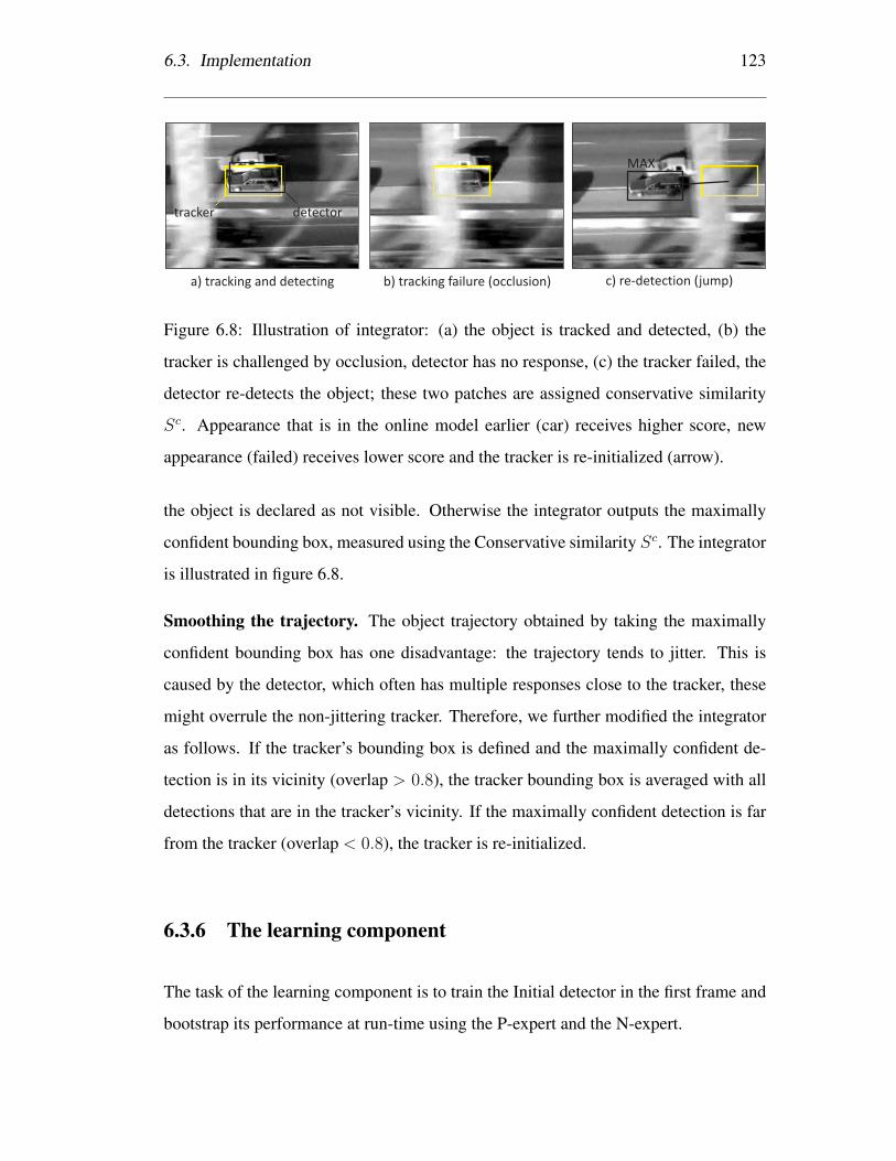
6.3. Implementation 123
c) re-detection (jump)b) tracking failure (occlusion)a) tracking and detecting
tracker detector
MAX
Figure 6.8: Illustration of integrator: (a) the object is tracked and detected, (b) the
tracker is challenged by occlusion, detector has no response, (c) the tracker failed, the
detector re-detects the object; these two patches are assigned conservative similarity
Sc. Appearance that is in the online model earlier (car) receives higher score, new
appearance (failed) receives lower score and the tracker is re-initialized (arrow).
the object is declared as not visible. Otherwise the integrator outputs the maximally
confident bounding box, measured using the Conservative similarity Sc. The integrator
is illustrated in figure 6.8.
Smoothing the trajectory. The object trajectory obtained by taking the maximally
confident bounding box has one disadvantage: the trajectory tends to jitter. This is
caused by the detector, which often has multiple responses close to the tracker, these
might overrule the non-jittering tracker. Therefore, we further modified the integrator
as follows. If the tracker’s bounding box is defined and the maximally confident de-
tection is in its vicinity (overlap > 0.8), the tracker bounding box is averaged with all
detections that are in the tracker’s vicinity. If the maximally confident detection is far
from the tracker (overlap < 0.8), the tracker is re-initialized.
6.3.6 The learning component
The task of the learning component is to train the Initial detector in the first frame and
bootstrap its performance at run-time using the P-expert and the N-expert.
124 Chapter 6. Tracking-Learning-Detection (TLD)
Initialization
The Initial detector is trained using labeled examples that are generated as follows.
The positive training examples are synthesized from the initial bounding box. First,
we select 10 bounding boxes from the scanning grid that are closest to the initial patch.
For each of the bounding boxes, 20 warped versions are generated. The parameters
of the warping are drawn randomly from a uniform distribution of shift ±1%, scale
change±1% and in-plane rotation±10◦. The warped patches are added with Gaussian
noise (σ = 5). The result is 200 synthetic positive patches. Negative patches are
collected from the surrounding of the initial patch, no synthetic negative examples are
generated. If the application requires fast initialization, the training examples are sub-
sampled. The labeled training patches are then update the object model as discussed
in subsection 6.3.2 and the ensemble classifier as discussed in subsection 6.3.3. After
the initialization, the Initial detector is ready for run-time.
The P-expert
The goal of the P-expert is to discover new appearances of the object and thus increase
the generality the object detector. Section 5.3 suggested a P-expert that exploits the
fact that the object moves on a trajectory. The object trajectory is generated by a
combination of the tracker, the detector and the integrator. This combined process
traces a discontinuous trajectory, which is by no means correct all the time as any of
the components can fail. The challenge of the P-expert is to estimate reliable parts of
the trajectory and use it to generate positive training examples.
Consider an object model represented as colored points in a feature space. Positive
examples are represented by red dots connected by a directed curve suggesting their
order, negative examples are black. Using the conservative similarity Sc, one can
define a subspace in the feature space, where Sc > θL. We refer to this subspace as the
core of the object model.

6.3. Implementation 125
The P-expert estimates the reliable parts of the trajectory as follows. The trajectory
becomes reliable as soon as it enters the core and remains reliable until is re-initialized
or the tracker declares its own failure. Any other trajectory is not considered by the
P-expert. The reliable trajectory generates positive examples that are then added to the
object model. See figure 6.9 for illustration.
Parameter θL defines the extend of the ”core”, influences the rate by which the trajecto-
ries are validated and hence the rate of learning. As we have seen in experiment 5.3.3,
high values may result in situation when no learning takes place. On the other hand
low value may lead to degradation of the classifier. The exact setting of the parameter
is data dependent however it turned out that θL = 0.70 works for majority of cases.
This parameter is used in all of our experiments.
In every frame, the P-expert outputs a decision about the reliability of the current loca-
tion output by the integrator. If the current location is reliable, the P-expert generates a
set of positive examples that update the object model and the ensemble classifier. First,
we select 10 bounding boxes from the scanning grid that are closest to the initial patch.
For each of the bounding boxes, 10 warped versions are generated. The parameters
of the warping are drawn randomly from a uniform distribution of shift ±1%, scale
change ±1% and in-plane rotation ±5◦. The warped patches are added with Gaussian
noise (σ = 5). This results in 100 synthetic positive examples for the ensemble clas-
sifier. For efficiency reasons, we consider only 10 patches for the update of the object
model.
The N-expert
The N-expert generates negative training examples with the aim to discriminate the
detector against background clutter. The key assumption of the N-expert is that the
object can occupy at most one location in the image. The N-expert is applied at the
same time as P-expert. In that case, patches that are far from current bounding box

126 Chapter 6. Tracking-Learning-Detection (TLD)
a) b) c)
core
Figure 6.9: Illustration of the P-expert: (a) an object model in a feature space and
the core (gray blob); (b) a non-reliable trajectory (dotted line) and a reliable trajectory
(thick line); (c) the object model and the core after the update.
(overlap < 0.2) are all labeled as negative.
6.4 Quantitative evaluation
This section reports on a set of quantitative experiments comparing the TLD1.0 with
relevant algorithms. The first two experiments evaluate the TLD1.0 on benchmark
data sets that are commonly used in the literature. In particular, the experiment in sec-
tion 6.4.1 extends the results reported in [Santner 10]. The experiment in section 6.4.2
extends the results from [Yu 08]. In both cases, a saturated performance is achieved.
Section 6.4.3 therefore introduces a more challenging data set and performs further
evaluation.
Every experiment in this section adopts the following evaluation protocol. A tracker is
initialized in the first frame of a sequence and tracks the selected object up to the end of
the sequence. The produced trajectory is then compared to ground truth. The particular
evaluation measure is specified in every experiment. TLD1.0 has been compared with
11 comparable algorithms on 19 benchmark sequences. See Appendix A for more
details about the algorithms and Appendix B for the sequences.

6.4. Quantitative evaluation 127
6.4.1 Comparison 1: CoGD
TLD1.0 was compared with results reported in [Yu 08], which reports on performance
of 5 trackers: (i) Incremental Visual Tracking (IVT) [Ross 07], (ii) Online Discrim-
inative Features (ODF) [Collins 05], (iii) Ensemble Tracking (ET) [Avidan 07], (iv)
Multiple Instance Learning (MILTrack) [Babenko 09], and (v) Co-trained Generative
and Discriminative tracker (CoGD) [Yu 08]). The evaluation was performed on 6 se-
quences that include full occlusions and disappearance of the object. CoGD [Yu 08]
clearly dominated on these sequences as it is capable of re-detection of the object. The
performance was assessed using the Number of successfully tracked frames, i.e. the
number of frames where overlap with a ground truth bounding box is larger than 50%.
Frames where the object were occluded were not counted. For instance, for a sequence
of 100 frames where the object is occluded in 20 frames, the best possible score is 80
frames.
Table 6.1 shows the results. TLD1.0 achieved the maximal possible score in all se-
quences and matched the performance of CoGD [Yu 08]. It was reported in [Yu 08]
that CoGD runs at 2 frames per second, and requires several frames (typically 6) for
initialization. In contrast, TLD1.0 requires just a single frame and runs at 20 frames
per second.
This experiment demonstrates that neither the generative trackers (IVT [Ross 07]), nor
the discriminative trackers (ODF [Collins 05], ET [Avidan 07], MILTrack [Babenko 09])
are able to handle long-lasting full occlusions or disappearance of the object. CoGD is
evaluated in detail on more challenging data in section 6.4.3.
6.4.2 Comparison 2: PROST
TLD1.0 was compared with the results reported in [Santner 10], which reports on per-
formance of 5 algorithms: (i) Online Boosting (OB) [Grabner 06], (ii) Online Random
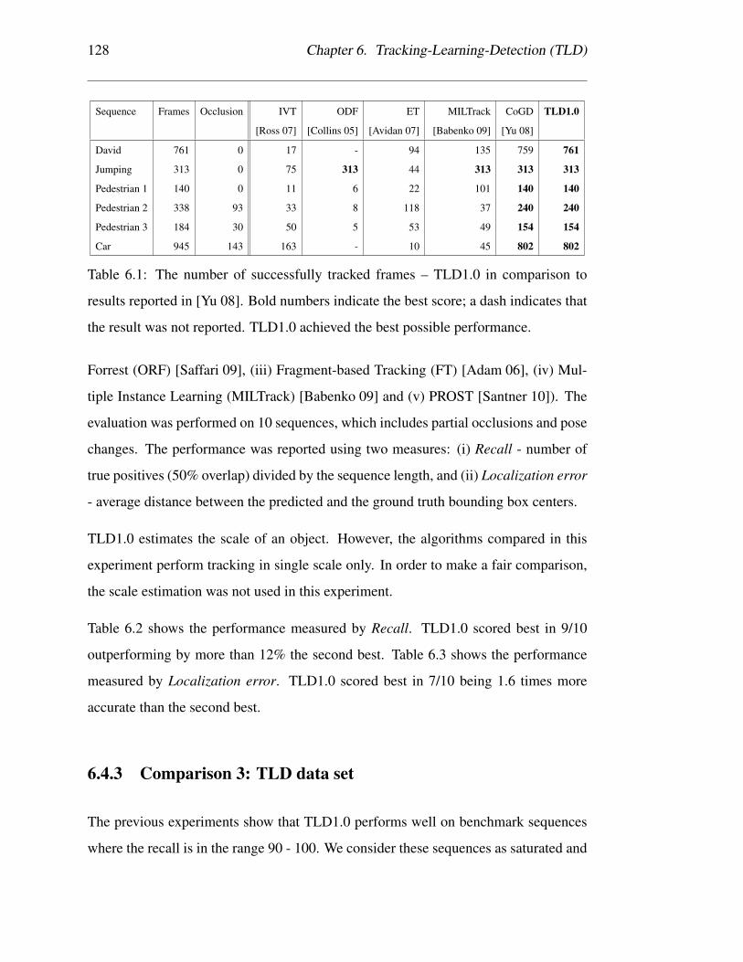
128 Chapter 6. Tracking-Learning-Detection (TLD)
Sequence Frames Occlusion IVT ODF ET MILTrack CoGD TLD1.0
[Ross 07] [Collins 05] [Avidan 07] [Babenko 09] [Yu 08]
David 761 0 17 - 94 135 759 761
Jumping 313 0 75 313 44 313 313 313
Pedestrian 1 140 0 11 6 22 101 140 140
Pedestrian 2 338 93 33 8 118 37 240 240
Pedestrian 3 184 30 50 5 53 49 154 154
Car 945 143 163 - 10 45 802 802
Table 6.1: The number of successfully tracked frames – TLD1.0 in comparison to
results reported in [Yu 08]. Bold numbers indicate the best score; a dash indicates that
the result was not reported. TLD1.0 achieved the best possible performance.
Forrest (ORF) [Saffari 09], (iii) Fragment-based Tracking (FT) [Adam 06], (iv) Mul-
tiple Instance Learning (MILTrack) [Babenko 09] and (v) PROST [Santner 10]). The
evaluation was performed on 10 sequences, which includes partial occlusions and pose
changes. The performance was reported using two measures: (i) Recall - number of
true positives (50% overlap) divided by the sequence length, and (ii) Localization error
- average distance between the predicted and the ground truth bounding box centers.
TLD1.0 estimates the scale of an object. However, the algorithms compared in this
experiment perform tracking in single scale only. In order to make a fair comparison,
the scale estimation was not used in this experiment.
Table 6.2 shows the performance measured by Recall. TLD1.0 scored best in 9/10
outperforming by more than 12% the second best. Table 6.3 shows the performance
measured by Localization error. TLD1.0 scored best in 7/10 being 1.6 times more
accurate than the second best.
6.4.3 Comparison 3: TLD data set
The previous experiments show that TLD1.0 performs well on benchmark sequences
where the recall is in the range 90 - 100. We consider these sequences as saturated and

6.4. Quantitative evaluation 129
Sequence Frames OnlineBoost OnlineRF FragTrack MILTrack Prost TLD1.0
[Grabner 06] [Saffari 09] [Adam 06] [Babenko 09] [Santner 10]
Girl 452 24.0 - 70.0 70.0 89.0 93.1
David 502 23.0 - 47.0 70.0 80.0 100.0
Sylvester 1344 51.0 - 74.0 74.0 73.0 97.4
Face occlusion 1 858 35.0 - 100.0 93.0 100.0 98.9
Face occlusion 2 812 75.0 - 48.0 96.0 82.0 96.9
Tiger 354 38.0 - 20.0 77.0 79.0 88.7
Board 698 - 10.0 67.9 67.9 75.0 87.1
Box 1161 - 28.3 61.4 24.5 91.4 91.8
Lemming 1336 - 17.2 54.9 83.6 70.5 85.8
Liquor 1741 - 53.6 79.9 20.6 83.7 91.7
Mean - 42.2 27.3 58.1 64.8 80.4 92.5
Table 6.2: Recall – TLD1.0 in comparison to results reported in [Santner 10]. Bold
numbers indicate the best score; a dash indicates that the result was not reported.
TLD1.0 scored best in 9/10 sequences.
Sequence Frames OnlineBoost OnlineRF FragTrack MILTrack PROST TLD1.0
[Grabner 06] [Saffari 09] [Adam 06] [Babenko 09] [Santner 10]
Girl 452 43.3 - 26.5 31.6 19.0 18.1
David 502 51.0 - 46.0 15.6 15.3 4.0
Sylvester 1344 32.9 - 11.2 9.4 10.6 5.9
Face occlusion 1 858 49.0 - 6.5 18.4 7.0 15.4
Face occlusion 2 812 19.6 - 45.1 14.3 17.2 12.6
Tiger 354 17.9 - 39.6 8.4 7.2 6.4
Board 698 - 154.5 154.5 51.2 37.0 10.9
Box 1161 - 145.4 145.4 104.5 12.1 17.4
Lemming 1336 - 166.3 166.3 14.9 25.4 16.4
Liquor 1741 - 67.3 67.3 165.1 21.6 6.5
Mean - 32.9 133.4 78.0 46.1 18.4 10.9
Table 6.3: Localization error (pixels) – TLD1.0 in comparison to results reported
in [Santner 10]. Bold numbers indicate the best score; a dash indicates that the re-
sult was not reported. TLD1.0 scored best in 7/10 sequences.

130 Chapter 6. Tracking-Learning-Detection (TLD)
intorduce new, more challenging ones.
The TLD data set consists of 10 sequences. The sequences 1-6 have been used in ex-
perimentt 6.4.1 and include: David, Jumping, Pedestrian 1, Pedestrian 2, Pedestrian 3
and Car. The sequences 7-10 are new and include: Motorbike, Volkswagen, Car Chase
and Panda. These sequences are long and contain all the challenges outlined in the
chapter 1. All sequences were manually annotated with ground truth. In every frame,
the object is defined by a bounding box or it is indicated that the object is not visi-
ble. More than 50% of occlusion or more than 90 degrees of out-of-plane rotation was
annotated as ”not visible”. See Appendix B for more details. The TLD data set is
available online at the website of the TLD project.1
Five tracking algorithms are compared on the TLD data set: (1) Online Boosting
(OB) [Grabner 06], (2) Semi-Supervised Online Boosting (SOB) [Grabner 08], (3)
Beyond Semi-Supervised Online Boosting (BSOB) [Stalder 09], (4) Multiple Instance
Learning (MILTrack) [Babenko 09], and (5) Co-trained Generative and Discrimina-
tive tracker (CoGD) [Yu 08]. Binaries for trackers (1-3) are available in the Internet2.
Tracker (4,5) were kindly evaluated directly by their authors.
The performance is evaluated using precision P , recall R and f-measure F . P is the
number of true positives divided by number of all responses, R is the number true
positivs divided by the number of object occurrences that should have been detected. F
combines these two measures as F = 2PR/(P +R). Since this experiment compares
various trackers for which the default initialization (defined by the ground truth) might
not be optimal, it was allowed to initialize the object arbitrarily. For instance, when
tracking a motorbike racer, some algorithms might perform better when tracking only
a part of the racer. Every trajectory was therefore normalized. A transformation that
mapped the initializing bounding box to the ground truth bounding box was found
(shift, aspect and scale) and this transformation was applied to every bounding box
1cmp.felk.cvut.cz/tld2http://www.vision.ee.ethz.ch/boostingTrackers/

6.4. Quantitative evaluation 131
Sequence Frames OB SOB BSOB MILTrack CoGD TLD1.0
[Grabner 06] [Grabner 08] [Stalder 09] [Babenko 09] [Yu 08]
David 761 0.34 0.35 0.28 0.15 1.00 1.00
Jumping 313 0.09 0.17 0.15 1.00 1.00 1.00
Pedestrian 1 140 0.23 0.39 0.15 0.69 1.00 1.00
Pedestrian 2 338 0.21 0.77 0.04 0.11 0.81 0.91
Pedestrian 3 184 0.49 0.36 0.62 0.75 0.92 0.99
Car 945 0.73 0.80 0.72 0.24 0.96 0.94
Motocross 2665 0.01 0.05 0.00 0.03 0.45 0.83
Volkswagen 8576 0.04 0.04 0.01 0.07 0.11 0.87
Carchase 9928 0.06 0.09 0.19 0.07 0.08 0.77
Panda 3000 0.51 0.29 0.30 0.38 0.12 0.60
mean 26850 0.13 0.14 0.15 0.13 0.22 0.81
Table 6.4: F-measure – performance on the TLD data set. Bold numbers indicate the
best score. TLD1.0 scored best in 9/10 sequences.
on the trajectory. The normalized trajectory was directly compared to ground truth
using overlap and a true positive was considered if the overlap was larger than 25%.
The earlier used threshold 50% was found to be too restrictive in this case. Sequences
Motocross and Volkswagen were evaluated by the MILTrack [Babenko 09] only up
to the frame 500 as the implementation required loading all images into memory in
advance. Since the algorithm failed during this period the remaining frames were
considered as failed.
Table 6.4 show the performance as measured by f-measure. The last row shows
a weighted average performance (weighted by number of frames in the sequence).
TLD1.0 achieved the best performance of 81% significantly outperforming the sec-
ond best approach that achieved 22%, other approaches range between 13-15%. The
performance is broken down to precision in table 6.5 and recall in table 6.6. This exper-
iment demonstrates that TLD1.0 significantly outperforms state-of-the-art approaches
on challenging data.
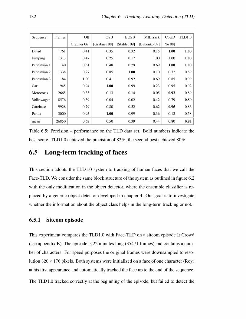
132 Chapter 6. Tracking-Learning-Detection (TLD)
Sequence Frames OB OSB BOSB MILTrack CoGD TLD1.0
[Grabner 06] [Grabner 08] [Stalder 09] [Babenko 09] [Yu 08]
David 761 0.41 0.35 0.32 0.15 1.00 1.00
Jumping 313 0.47 0.25 0.17 1.00 1.00 1.00
Pedestrian 1 140 0.61 0.48 0.29 0.69 1.00 1.00
Pedestrian 2 338 0.77 0.85 1.00 0.10 0.72 0.89
Pedestrian 3 184 1.00 0.41 0.92 0.69 0.85 0.99
Car 945 0.94 1.00 0.99 0.23 0.95 0.92
Motocross 2665 0.33 0.13 0.14 0.05 0.93 0.89
Volkswagen 8576 0.39 0.04 0.02 0.42 0.79 0.80
Carchase 9928 0.79 0.80 0.52 0.62 0.95 0.86
Panda 3000 0.95 1.00 0.99 0.36 0.12 0.58
mean 26850 0.62 0.50 0.39 0.44 0.80 0.82
Table 6.5: Precision – performance on the TLD data set. Bold numbers indicate the
best score. TLD1.0 achieved the precision of 82%, the second best achieved 80%.
6.5 Long-term tracking of faces
This section adopts the TLD1.0 system to tracking of human faces that we call the
Face-TLD. We consider the same block structure of the system as outlined in figure 6.2
with the only modification in the object detector, where the ensemble classifier is re-
placed by a generic object detector developed in chapter 4. Our goal is to investigate
whether the information about the object class helps in the long-term tracking or not.
6.5.1 Sitcom episode
This experiment compares the TLD1.0 with Face-TLD on a sitcom episode It Crowd
(see appendix B). The episode is 22 minutes long (35471 frames) and contains a num-
ber of characters. For speed purposes the original frames were downsampled to reso-
lution 320×176 pixels. Both systems were initialized on a face of one character (Roy)
at his first appearance and automatically tracked the face up to the end of the sequence.
The TLD1.0 tracked correctly at the beginning of the episode, but failed to detect the
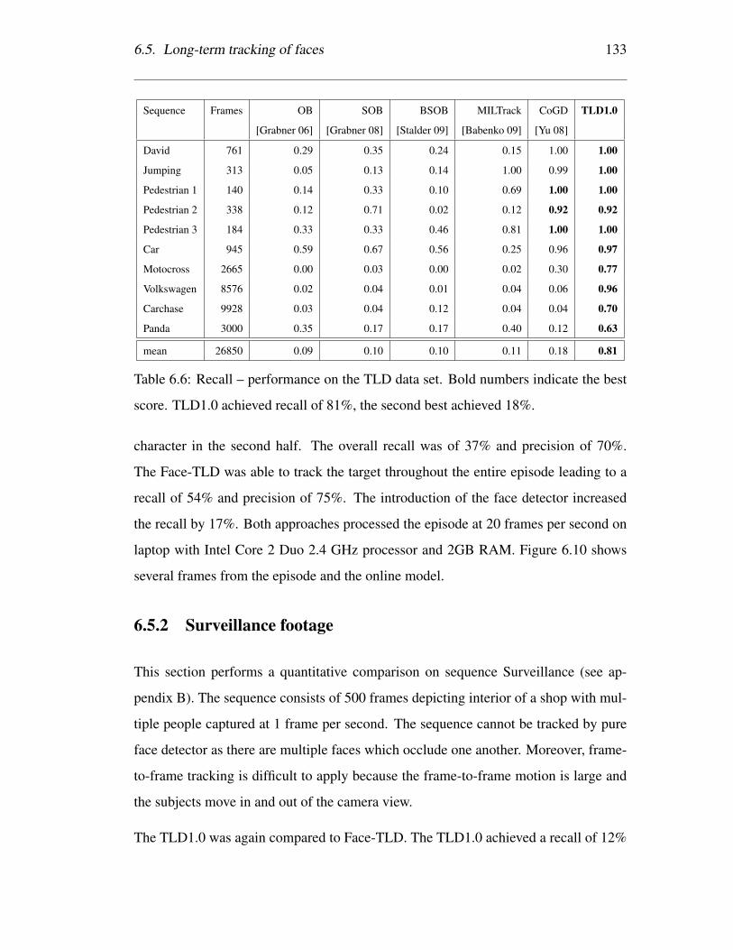
6.5. Long-term tracking of faces 133
Sequence Frames OB SOB BSOB MILTrack CoGD TLD1.0
[Grabner 06] [Grabner 08] [Stalder 09] [Babenko 09] [Yu 08]
David 761 0.29 0.35 0.24 0.15 1.00 1.00
Jumping 313 0.05 0.13 0.14 1.00 0.99 1.00
Pedestrian 1 140 0.14 0.33 0.10 0.69 1.00 1.00
Pedestrian 2 338 0.12 0.71 0.02 0.12 0.92 0.92
Pedestrian 3 184 0.33 0.33 0.46 0.81 1.00 1.00
Car 945 0.59 0.67 0.56 0.25 0.96 0.97
Motocross 2665 0.00 0.03 0.00 0.02 0.30 0.77
Volkswagen 8576 0.02 0.04 0.01 0.04 0.06 0.96
Carchase 9928 0.03 0.04 0.12 0.04 0.04 0.70
Panda 3000 0.35 0.17 0.17 0.40 0.12 0.63
mean 26850 0.09 0.10 0.10 0.11 0.18 0.81
Table 6.6: Recall – performance on the TLD data set. Bold numbers indicate the best
score. TLD1.0 achieved recall of 81%, the second best achieved 18%.
character in the second half. The overall recall was of 37% and precision of 70%.
The Face-TLD was able to track the target throughout the entire episode leading to a
recall of 54% and precision of 75%. The introduction of the face detector increased
the recall by 17%. Both approaches processed the episode at 20 frames per second on
laptop with Intel Core 2 Duo 2.4 GHz processor and 2GB RAM. Figure 6.10 shows
several frames from the episode and the online model.
6.5.2 Surveillance footage
This section performs a quantitative comparison on sequence Surveillance (see ap-
pendix B). The sequence consists of 500 frames depicting interior of a shop with mul-
tiple people captured at 1 frame per second. The sequence cannot be tracked by pure
face detector as there are multiple faces which occlude one another. Moreover, frame-
to-frame tracking is difficult to apply because the frame-to-frame motion is large and
the subjects move in and out of the camera view.
The TLD1.0 was again compared to Face-TLD. The TLD1.0 achieved a recall of 12%
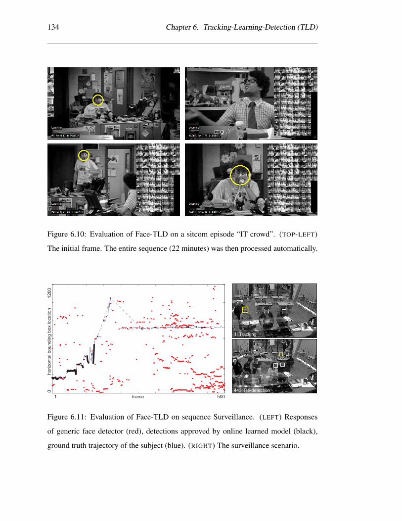
134 Chapter 6. Tracking-Learning-Detection (TLD)
Figure 6.10: Evaluation of Face-TLD on a sitcom episode “IT crowd”. (TOP-LEFT)
The initial frame. The entire sequence (22 minutes) was then processed automatically.
1: Tracking
443: Re-detection
500
01
20
0
frame
ho
rizo
nta
l b
ou
nd
ing
bo
x lo
ca
tio
n
1
Figure 6.11: Evaluation of Face-TLD on sequence Surveillance. (LEFT) Responses
of generic face detector (red), detections approved by online learned model (black),
ground truth trajectory of the subject (blue). (RIGHT) The surveillance scenario.

6.6. Qualitative analysis 135
and a precision of 57%, the Face-TLD achieved a recall of 35% and a precision of
79%. The introduction of face detector increased the recall by 23%. Figure 6.11
illustrates the scenario. This experiment demonstrates, that both TLD1.0 and Face-
TLD are applicable to surveillance scenarios for tracking of faces. Furthermore, it
shows that using a face detector increases the performance of the TLD system.
6.6 Qualitative analysis
This section discusses the strengths and weaknesses of TLD1.0 with respect to the
challenges outlined in the chapter 1. The performance is illustrated on several snap-
shots from run-time of the system, where the following marking is used:
• Yellow rectangle - the bounding box output of the TLD1.0,
• Gray dots - detections output by the second stage of our detector,
• Red dots - detections output by the whole detector,
• Blue dots - the reliable points used by the Median-Flow tracker,
• Patches to the left - negative examples in the online model,
• Patches to the right - positive examples in the online model.
• Top left corner depict close-up of the object.
6.6.1 Strengths
Scale changes. TLD1.0 is robust to scale changes. Median-Flow estimates scale
changes even when the target is partially out of the frame. Detector localizes the ob-
ject in multiple scales. In sequence Volkswagen, the object of interest changes scale

136 Chapter 6. Tracking-Learning-Detection (TLD)
Figure 6.12: TLD1.0 and scale changes.
Figure 6.13: TLD1.0 and illumination changes.
in the range from 20x20 to 100x100 pixels. The output of TLD1.0 is illustrated in
figure 6.12.
Illumination changes. TLD1.0 is invariant to smooth changes in illumination. Median-
Flow adapts the tracked templates and the detector is based on illumination invariant
pixel comparisons and NCC. In sequence David, a face is tracked from a dark room to
full illumination. Figure 6.13 shows the results.
Appearance changes. Median-Flow handles changes of appearance caused by pose
change or articulations. The detector localizes all appearances observed in the past.
In sequence Motocross, TLD1.0 learned all appearances of a motorbike from the rear
view. However, it did not learn the side view. The detector was therefore not able to
re-initialize a trajectory in that case. See figure 6.14 for illustration.
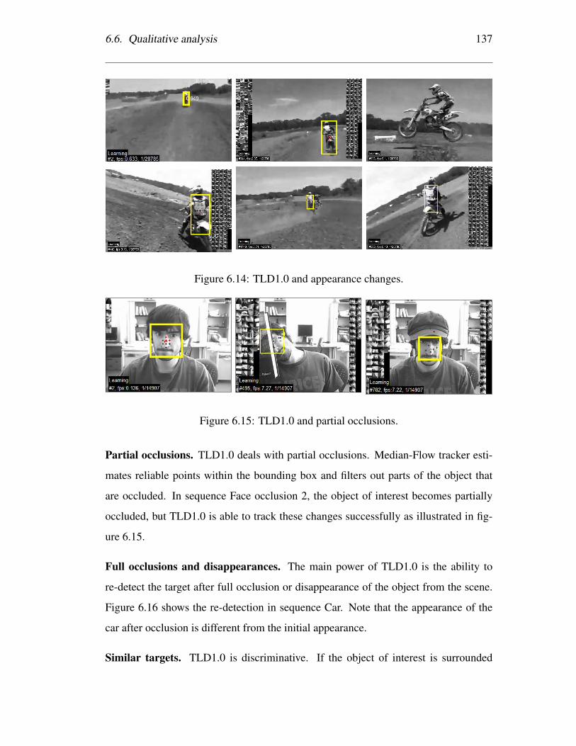
6.6. Qualitative analysis 137
Figure 6.14: TLD1.0 and appearance changes.
Figure 6.15: TLD1.0 and partial occlusions.
Partial occlusions. TLD1.0 deals with partial occlusions. Median-Flow tracker esti-
mates reliable points within the bounding box and filters out parts of the object that
are occluded. In sequence Face occlusion 2, the object of interest becomes partially
occluded, but TLD1.0 is able to track these changes successfully as illustrated in fig-
ure 6.15.
Full occlusions and disappearances. The main power of TLD1.0 is the ability to
re-detect the target after full occlusion or disappearance of the object from the scene.
Figure 6.16 shows the re-detection in sequence Car. Note that the appearance of the
car after occlusion is different from the initial appearance.
Similar targets. TLD1.0 is discriminative. If the object of interest is surrounded

138 Chapter 6. Tracking-Learning-Detection (TLD)
Figure 6.16: TLD1.0 and re-detection.
Figure 6.17: TLD1.0 and similar targets. The sequence appeared in [Kwon 10].
by objects of similar appearance or background clutter, the N-expert labels them as
negative and inserts them to the online model. These negative examples then prevent
the detector from confusing the object of interest with other objects. For instance in
figure 6.17 the object of interest is a helmet of a football player. Notice that various
appearances of the same helmet appear in positive examples, whereas different helmets
occur in negative examples. This is best visible when zooming in on a display.
6.6.2 Weaknesses
Out-of-plane rotations. In case of out-of-plane rotation, Median-flow drifts away
from the target. The tracker typically stays away until a detector re-initializes its posi-
tion to previously seen appearance. For instance, figure 6.18 shows a sequence of an
object performing out-of-plane rotation. From frame 1 to 168, the object performs out
of plane rotation and the Median-Flow drifts. As the drift is slow, the failure of the
tracker is not identified and the system is learning new incorrect appearances. In frame
176 the object re-appears in previously seen appearance and the trajectory is correctly

6.6. Qualitative analysis 139
Figure 6.18: Out-of-plane rotations are challenging for TLD1.0. The sequence ap-
peared in [Leichter 09].
Figure 6.19: TLD1.0 and sequences where the object never re-appear in a similar view.
The sequence appeared in [Kwon 10].
re-initialized. Notice that the incorrect data produced by the drift did not prevent the
tracker from correct re-initialization of the trajectory.
No previously seen appearances. Particularly challenging scenarios for TLD1.0 are
scenes when the object never re-appears in previously observed appearance. For in-
stance, figure 6.19 shows an example when tracking a face in a Soccer sequence
from [Kwon 10]. The target object is tracked for a couple of frames but then fails
due to occlusion combined with pose and expression changes. The target is never
re-detected as the object never re-appears with previously observed appearance.

140 Chapter 6. Tracking-Learning-Detection (TLD)

Chapter 7
Discussion
This chapter discusses the contributions of the thesis, reviews recent developments,
and proposes possible avenues for future research.
7.1 Contributions
In this thesis, we have proposed a new paradigm for long-term tracking of unknown
objects. Our approach was demonstrated on a number of challenging videos, and sig-
nificantly outperformed state-of-the-art. The particular contributions are summarized
below.
In chapter 3, we studied the long-term tracking problem from the perspective of frame-
to-frame tracking. We accepted that frame-to-frame tracking is not a good model for
this scenario as it leads to inevitable failures. Rather than trying to avoid these failures
by directly designing a better frame-to-frame tracker, we proposed a novel measure that
indicates the reliability of a tracker. The measure is based on the well known forward-
backward consistency assumption. We demonstrated that the proposed measure pro-
vides complementary information to appearance-based NNC and SSD. Furthermore,
we used the error measure to improve frame-to-frame tracking itself. We showed that
141
142 Chapter 7. Discussion
template tracking can be improved if the template is decomposed into independently
tracked parts which are weighted based on their reliability and integrated using median
estimator. The result is a novel template-based tracker (Median-Flow) which is robust
to partial occlusions and appearance changes and outperforms comparable approaches.
In chapter 4, we studied the long-term tracking problem from the perspective of tracking-
by-detection. We developed a novel learning method for supervised training of an
object detector from a large data set. In particular, we focused on learning methods
that combine bootstrapping and boosting. The theoretical contribution is the formal-
ization of bootstrapping and boosting in a unified framework. Within this framework,
we designed the optimal combination of the two approaches. The approach formulates
bootstrapping as a weighted sampling where the weights are driven by boosting. The
resulting combination demonstrated a significant improvement in terms of efficiency
(both in training and testing) as well as the classifier accuracy in contrast to ad hoc
combinations. The learning method has been applied to training face detectors (frontal
and profile), which operate at video frame-rate on QVGA images. Such detectors are
relevant to all long-term tracking scenarios, where the target object is a face. The
learning method does not make any face-specific assumptions and can be applied to
any other visual classes.
In chapter 5, we investigated the task of learning during long-term tracking. We have
demonstrated that an accurate object detector can be trained from a single example
and an unlabeled video stream using the following strategy: (i) evaluate the detector,
(ii) estimate its errors, and (iii) update the detector. The main novelty of the method
is the estimation of the detector errors, which is guided by two rules, which we call
the P-expert and N-expert, respectively. P-expert estimates only false negatives and
improves the detector generality. N-expert estimates only false positives and increases
the detector discriminability. Estimation of the detector’s errors independently based
on their type enabled not only simpler design of the experts, but also mutual compen-
sation of their errors. The theoretical contribution is the formalization of this learning

7.2. Recent development 143
process as a discrete dynamical system, which allowed us to specify conditions, under
which the learning guarantees improvement of the detector. We demonstrated, that the
experts can be designed when considering spatio-temporal relationships in the video.
In chapter 6, we proposed a novel tracking framework (TLD) that decomposes the
long-term tracking task into three sub-tasks: tracking, learning and detection. Build-
ing on the components developed in chapters 3, 4 and 5, we showed how to implement
the TLD framework and how to achieve real-time performance. An extensive quantita-
tive evaluation on benchmark sequences demonstrated saturated performance. There-
fore, we introduced a new data set, ground truth and evaluation protocol and showed
a significant improvement over state-of-the-art approaches. Finally, we applied TLD
to the tracking of human faces and demonstrated how to incorporate an offline trained
detector to further improve long-term tracking.
7.2 Recent development
The source code of TLD1.0 has been released under GPL v3.0 license and is available
online 1. A corresponding discussion group has currently over 1000 registered users.
A presentation video2 that explains TLD crossed 0.5 million hits within one month on
YouTube and caused a lot of attention for TLD from academia, industry and media.
Moreover the author has been invited to give a Google Tech Talk 3.
The implementation of TLD has been demonstrated at Computer Vision and Pattern
Recognition, 2010. The system has been running for more than 8 hours, tracking vari-
ous objects in real-time. Figure 7.1 shows the setup of the demo and several snapshots
taken automatically from the demo camera.
1https://github.com/zk00006/OpenTLD2http://youtu.be/1GhNXHCQGsM3http://youtu.be/lmG FjG4Dy8
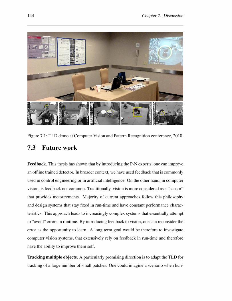
144 Chapter 7. Discussion
Figure 7.1: TLD demo at Computer Vision and Pattern Recognition conference, 2010.
7.3 Future work
Feedback. This thesis has shown that by introducing the P-N experts, one can improve
an offline trained detector. In broader context, we have used feedback that is commonly
used in control engineering or in artificial intelligence. On the other hand, in computer
vision, is feedback not common. Traditionally, vision is more considered as a “sensor”
that provides measurements. Majority of current approaches follow this philosophy
and design systems that stay fixed in run-time and have constant performance charac-
teristics. This approach leads to increasingly complex systems that essentially attempt
to ”avoid” errors in runtime. By introducing feedback to vision, one can reconsider the
error as the opportunity to learn. A long term goal would be therefore to investigate
computer vision systems, that extensively rely on feedback in run-time and therefore
have the ability to improve them self.
Tracking multiple objects. A particularly promising direction is to adapt the TLD for
tracking of a large number of small patches. One could imagine a scenario when hun-

7.3. Future work 145
dreds of points are tracked simultaneously, each of which has the property to learn its
appearance on the fly, detect its disappearance and re-initialize its own trajectory when
it becomes visible. Such an approach would be applicable in a number of applications.
Extension of the ideas of TLD to optical flow is also an very promising direction that
is becoming realistic with the increasing speed of processors and availability of GPU.
Tracking. In chapter 7, we have demonstrated that a relatively simple tracker coupled
with a learning method and detector, significantly outperforms competing approaches.
On the other hand, we observed that if the tracker fails too quickly (e.g. due to out-
of-plain rotation), the detector is not able to re-initialize the tracker. Therefore one
promising way to proceed is to strengthen the tracking itself, e.g. by running multiple
trackers in parallel [Kwon 10] each of which would be based on different features and
motion models. Such an approach would lead to a set of P-experts that would train the
detector more quickly.
Detection. The detector used in our system is based on a scanning window and
global representation of the object and as such is prone to occlusions. However, as
we have reviewed in chapter 2, a number of detectors are based on local representa-
tions [Lowe 04] where partial occlusions are not an issue.
Learning. In chapter 5, we proposed a learning method (P-N Learning) which pro-
cesses a video stream in one pass, considering only one frame at a time. Frames
observed in the past were not used. While our motivation was mainly speed, this is
no longer an issue for a multi-threaded architecture. One can imagine a second thread
analysing the already processed frames, thus providing more training data for the de-
tector. In an ideal case, the detector should reflect all the information received up to
current time.
Faster implementation. While the current implementation of TLD1.0 is running in
real-time on QVGA images, for larger images the frame-rate drops since the detector
has to evaluate a larger number of windows. A GPU implementation is a potential way

146 Chapter 7. Discussion
to increase the speed as the scanning window approach can be parallelized. Implemen-
tation of pieces of code using SSE instruction set is also a promising direction.
Apply P-N Learning to other problems. In chapter 5, P-N Learning was applied
to data from a video stream with a specific spatio-temporal structure. The structure
is, however, present in many other problems as well. One possible way is to exploit
search engines such as Google Image Search. Search for a particular object (e.g. a
dog) returns a set of images where the object is likely to appear (P-expert). A search
for other object categories returns a set of images where the object is typically not
present (N-expert).
Sophisticated experts. The P-N experts used in this thesis are relatively simple, as
they were describing motion of a single object in a video stream. Apart from the
assumption that the object is unique in the image and the object moves on a trajectory,
the experts did not take any other assumption. In more complex scenarios, e.g. when
tracking multiple object in parallel, one can formalise more complex rules to describe
the problem.

Appendix A
Compared algorithms
1. FT: Fragment-based Tracker [Adam 06], a static template tracker which repre-
sents the object by a set of parts. In presence of partial occlusions, the method
have demonstrated better performance than Mean-Shift [Comaniciu 03].
2. IVT: Incremental Visual Tracking [Ross 07], a particle filter that incrementally
builds a PCA-based model of the object.
3. ET: Ensemble Tracking [Avidan 07], a mean shift-based tracker that adapts an
discriminative model classifying pixels.
4. ODF: Online Discriminative Features [Collins 03], a mean shift-based tracker
that adapts color projections to separate the object from background.
5. OB: Online Boosting Tracker [Grabner 06], an approach similar to ODF, but the
classification is performed on bounding box level.
6. ORF: Online Random Forests [Saffari 09], an approach similar to OB but more
robust with respect to noise.
7. SOB: Semi-supervised Online Boosting [Grabner 08], an extension of OB that
internally trains 2 classifiers.
147

148 Appendix A. Compared algorithms
8. BSOB: Beyond Semi-supervised Online Boosting [Stalder 09], an extension of
SOB that trains 3 classifiers to simultaneously increase adaptability and stability.
9. MILTrack: Multiple Instance Learning tracker [Babenko 09], an approach sim-
ilar to OB but with a modified, drift-resistant updating strategy.
10. CoGD: Co-trained Generative and Discriminative [Yu 08], a particle filter that
co-trains a pair of classifiers.
11. PROST: Parallel Robust Online Simple Tracking [Santner 10], a method based
on three complementary trackers: template, optical flow and random forest.

Appendix B
Sequences used for evaluation
The TLD1.0 system has been quantitatively evaluated on 21 sequences specified in
table B.1 and shown in figure B.1.
149

150 Appendix B. Sequences used for evaluation
Table B.1: Description of sequences used for evaluation. A horizontal line separates
the standard and the introduced sequences. The red color indicates sequences from the
TLD data set.

151
1) Girl
2) David
3) Syklvestr
4) Face occlusion 1
5) Face occlusion 2
6) Tiger
7) Board
8) Box
9) Lemming
10) Liquor
11) Jumping
12) Pedestrian 1
13) Pedestrian 2
14) Pedestrian 3
15) Car
16) Motocross
17) Volkswagen
19) Panda
18) Car Chase
20) IT Crowd
21) Surveillance
Figure B.1: Snapshots from the sequences used for evaluation. A horizontal line sepa-
rates the standard and the introduced sequences.

152 Appendix B. Sequences used for evaluation

Bibliography
[Adam 06] A. Adam, E. Rivlin & I. Shimshoni. Robust Fragments-based
Tracking using the Integral Histogram. Conference on Computer
Vision and Pattern Recognition, pages 798–805, 2006.
[Aha 91] D W Aha, D Kibler & M K Albert. Instance-based learning al-
gorithms. Machine Learning, vol. 6, no. 1, pages 37–66, 1991.
[Alvarez 07] L Alvarez, R Deriche, T Papadopoulo & J Sanchez. Symmetrical
dense optical flow estimation with occlusions detection. Interna-
tional Journal of Computer Vision, vol. 75, no. 3, pages 371–385,
2007.
[Amit 97] Y Amit & D Geman. Shape quantization and recognition with
randomized trees. Neural computation, vol. 9, no. 7, pages 1545–
1588, 1997.
[Avidan 04] S Avidan. Support Vector Tracking. IEEE Transactions on Pattern
Analysis and Machine Intelligence, pages 1064–1072, 2004.
[Avidan 07] S Avidan. Ensemble Tracking. IEEE Transactions on Pattern
Analysis and Machine Intelligence, vol. 29, no. 2, pages 261–271,
2007.
[Babenko 09] B Babenko, Ming-Hsuan Yang & S Belongie. Visual Tracking
153

154 Bibliography
with Online Multiple Instance Learning. Conference on Com-
puter Vision and Pattern Recognition, 2009.
[Baker 04] S Baker & I Matthews. Lucas-Kanade 20 Years On: A Unifying
Framework. International Journal of Computer Vision, vol. 56,
no. 3, pages 221–255, February 2004.
[Barron 94] J L Barron, D J Fleet & S S Beauchemin. Performance of Opti-
cal Flow Techniques. International Journal of Computer Vision,
vol. 12, no. 1, pages 43–77, 1994.
[Belhumeur 97] P Belhumeur, J Hespanha & D Kriegman. Eigenfaces vs. Fish-
erfaces: recognition using class specific linearprojection. IEEE
Transactions on Pattern Analysis and Machine Intelligence, 1997.
[Bibby 08] C Bibby & I Reid. Robust real-time visual tracking using pixel-
wise posteriors. European Conference on Computer Vision, 2008.
[Bibby 10] C Bibby & I Reid. Real-time Tracking of Multiple Occluding Ob-
jects using Level Sets. Computer Vision and Pattern Recognition,
2010.
[Birchfield 98] S Birchfield. Elliptical head tracking using intensity gradients
and color histograms. Conference on Computer Vision and Pat-
tern Recognition, 1998.
[Black 98] M J Black & A D Jepson. Eigentracking: Robust matching and
tracking of articulated objects using a view-based representation.
International Journal of Computer Vision, vol. 26, no. 1, pages
63–84, 1998.
[Blum 98] A Blum & T Mitchell. Combining labeled and unlabeled data
with co-training. Conference on Computational Learning Theory,
page 100, 1998.

Bibliography 155
[Bouguet 99] J Y Bouguet. Pyramidal Implementation of the Lucas Kanade
Feature Tracker Description of the algorithm. Technical Report,
Intel Microprocessor Research Labs, 1999.
[Bradski 98] G R Bradski. Computer vision face tracking for use in a percep-
tual user interface. Intel Technology Journal, vol. 2, no. 2, pages
12–21, 1998.
[Breiman 96] L Breiman. Bagging predictors. Machine Learning, vol. 24, no. 2,
pages 123–140, 1996.
[Breiman 01] L Breiman. Random forests. Machine Learning, vol. 45, no. 1,
pages 5–32, 2001.
[Brox 04] T Brox, A Bruhn, N Papenberg & J Weickert. High accuracy
optical flow estimation based on a theory for warping. European
Conference on Computer Vision, pages 25–36, 2004.
[Buchanan 06] A. M. Buchanan & A. W. Fitzgibbon. Interactive Feature Track-
ing using K-D Trees and Dynamic Programming. In IEEE Con-
ference on Computer Vision and Pattern Recognition, volume 1,
pages 626–633, 2006.
[Buehler 08] P Buehler, M Everingham, D P Huttenlocher & A Zisserman.
Long term arm and hand tracking for continuous sign language
TV broadcasts. British Machine Vision Conference, 2008.
[Calonder 08] M Calonder, V Lepetit & P Fua. Keypoint signatures for fast
learning and recognition. European Conference on Computer Vi-
sion, pages 58–71, 2008.
[Calonder 10] M Calonder, V Lepetit & P Fua. BRIEF : Binary Robust Indepen-
dent Elementary Features. European Conference on Computer
Vision, 2010.

156 Bibliography
[Cauwenberghs 01] G Cauwenberghs & T Poggio. Incremental and decremental sup-
port vector machine learning. Advances in neural information
processing systems, page 409, 2001.
[Chapelle 06] O Chapelle, B Scholkopf & A Zien. Semi-Supervised Learning.
MIT Press, Cambridge, MA, 2006.
[Collins 03] R Collins & Y Liu. On-line selection of discriminative tracking
features. Proceedings Ninth IEEE International Conference on
Computer Vision, pages 346–352 vol.1, 2003.
[Collins 05] R Collins, Y Liu & M Leordeanu. Online Selection of Discrim-
inative Tracking Features. IEEE Transactions on Pattern Analy-
sis and Machine Intelligence, vol. 27, no. 10, pages 1631–1643,
2005.
[Comaniciu 03] D Comaniciu, V Ramesh & P Meer. Kernel-Based Object Track-
ing. IEEE Transactions on Pattern Analysis and Machine Intelli-
gence, vol. 25, no. 5, pages 564–577, 2003.
[Dalal 05] N Dalal & B Triggs. Histograms of oriented gradients for human
detection. Conference on Computer Vision and Pattern Recogni-
tion, 2005.
[Davison 03] A J Davison. Real-time simultaneous localisation and mapping
with a single camera. International Conference on Computer Vi-
sion, 2003.
[Dietterich 97] T G Dietterich, R H Lathrop & T Lozano-Perez. Solving the mul-
tiple instance problem with axis-parallel rectangles. Artificial In-
telligence, vol. 89, no. 1-2, pages 31–71, 1997.

Bibliography 157
[Dowson 05] N Dowson & R Bowden. Simultaneous Modeling and Tracking
(SMAT) of Feature Sets. Conference on Computer Vision and
Pattern Recognition, 2005.
[Dowson 06] N Dowson & R. Bowden. N-tier simultaneous modelling and
tracking for arbitrary warps. In British Machine Vision Confer-
ence., 2006.
[Dowson 08] N Dowson & R Bowden. Mutual information for Lucas-Kanade
Tracking (MILK): an inverse compositional formulation. IEEE
transactions on pattern analysis and machine intelligence, vol. 30,
no. 1, pages 180–5, January 2008.
[Efron 93] B Efron & R Tibshirani. An Introduction to the Bootstrap. Chap-
man & Hall/CRC, 1993.
[Fergus 03] R Fergus, P Perona & A Zisserman. Object class recognition by
unsupervised scale-invariant learning. Conference on Computer
Vision and Pattern Recognition, vol. 2, 2003.
[Fischler 73] M A Fischler & R A Elschlager. The representation and match-
ing of pictorial structures. IEEE Transactions on Computers,
vol. 100, no. 22, pages 67–92, 1973.
[Fleuret 01] F Fleuret & D Geman. Coarse-to-Fine Face Detection. Interna-
tional Journal of Computer Vision, 2001.
[Fleuret 08] F Fleuret & D Geman. Stationary features and cat detection.
Journal of Machine Learning Research, vol. 9, pages 2549–2578,
2008.
[Freund 95] Y Freund. Boosting a weak learning algorithm by majority. In-
formation and Computation, 1995.

158 Bibliography
[Freund 97] Y Freund & R E Schapire. A Decision-Theoretic Generalization
of On-Line Learning and an Application to Boosting,. Journal of
Computer and System Sciences, vol. 55, no. 1, pages 119–139,
August 1997.
[Freund 01] Y Freund. An Adaptive Version of the Boost by Majority Algo-
rithm. Machine Learning, 2001.
[Friedman 00] J Friedman, T Hastie & R Tibshirani. Additive logistic regression:
a statistical view of boosting (With discussion and a rejoinder by
the authors). The Annals of Statistics, vol. 28, no. 2, pages 337–
407, 2000.
[Goldman 07] D B Goldman, B Curless, D Salesin & S M Seitz. Interactive
Video Object Annotation. ACM Computing Surveys, pages 1–7,
2007.
[Grabner 06] H Grabner & H Bischof. On-line boosting and vision. Conference
on Computer Vision and Pattern Recognition, 2006.
[Grabner 08] H Grabner, C Leistner & H Bischof. Semi-Supervised On-line
Boosting for Robust Tracking. European Conference on Com-
puter Vision, 2008.
[Hadid 04] A Hadid, M Pietikainen & T Ahonen. A Discriminative Feature
Space for Detecting and Recognizing Faces. IEEE Computer So-
ciety, no. ii, 2004.
[Harris 88] Ch Harris & M Stephens. A Combined Corner and Edge Detector.
Alvey vision conference, vol. 15, page 50, 1988.
[Hinterstoisser 09] S Hinterstoisser, O Kutter, N Navab, P Fua & V Lepetit. Real-time
learning of accurate patch rectification. Conference on Computer
Vision and Pattern Recognition, 2009.

Bibliography 159
[Hinterstoisser 10] S Hinterstoisser, V Lepetit, S Ilic, P Fua & N Navab. Dominant
Orientation Templates for Real-Time Detection of Texture-Less
Objects. Conference on Computer Vision and Pattern Recogni-
tion, 2010.
[Horn 81] B K P Horn & B G Schunck. Determining optical flow. Artificial
intelligence, vol. 17, no. 1-3, pages 185–203, 1981.
[Huang 07] C Huang, H Ai, Y Li & S Lao. High-Performance Rotation In-
variant Multiview Face Detection. IEEE Transactions on Pattern
Analysis and Machine Intelligence, 2007.
[Isard 98] M Isard & A Blake. CONDENSATION - Conditional Density
Propagation for Visual Tracking. International Journal of Com-
puter Vision, vol. 29, no. 1, pages 5–28, 1998.
[Javed 05] O Javed, S Ali & M Shah. Online detection and classification of
moving objects using progressively improving detectors. Confer-
ence on Computer Vision and Pattern Recognition, 2005.
[Jepson 03] A D Jepson, D J Fleet & T F El-Maraghi. Robust Online Appear-
ance Models for Visual Tracking. IEEE Transactions on Pattern
Analysis and Machine Intelligence, pages 1296–1311, 2003.
[Jones 03] M Jones & P Viola. Fast multi-view face detection. Conference
on Computer Vision and Pattern Recognition, 2003.
[Klein 07] G Klein & D Murray. Parallel Tracking and Mapping for Small
AR Workspaces. International Symposium on Mixed and Aug-
mented Reality, November 2007.
[Kolsch 04] M. Kolsch & M. Turk. Fast 2D Hand Tracking with Flocks of
Features and Multi-Cue Integration. Conference on Computer
Vision and Pattern Recognition Workshop, 2004.

160 Bibliography
[Kwon 10] J Kwon & K M Lee. Visual Tracking Decomposition. Conference
on Computer Vision and Pattern Recognition, 2010.
[Laptev 06] I Laptev. Improvements of object detection using boosted his-
tograms. British Machine Vision Conference, 2006.
[Leibe 07] B Leibe, K Schindler & L Van Gool. Coupled Detection and Tra-
jectory Estimation for Multi-Object Tracking. 2007 IEEE 11th
International Conference on Computer Vision, pages 1–8, Octo-
ber 2007.
[Leichter 09] I Leichter, M Lindenbaum & E Rivlin. Tracking by affine kernel
transformations using color and boundary cues. IEEE transac-
tions on pattern analysis and machine intelligence, vol. 31, no. 1,
pages 164–71, January 2009.
[Lepetit 05] V Lepetit, P Lagger & P Fua. Randomized trees for real-time
keypoint recognition. Conference on Computer Vision and Pattern
Recognition, 2005.
[Lepetit 06] V Lepetit & P Fua. Keypoint recognition using randomized trees.
IEEE transactions on pattern analysis and machine intelligence,
vol. 28, no. 9, pages 1465–79, September 2006.
[Levi 04] K Levi & Y Weiss. Learning object detection from a small num-
ber of examples: the importance of good features. Conference on
Computer Vision and Pattern Recognition, 2004.
[Levin 03] A Levin, P Viola & Y Freund. Unsupervised improvement of
visual detectors using co-training. International Conference on
Computer Vision, 2003.

Bibliography 161
[Lewis 94] D Lewis & W Gale. Training text classifiers by uncertainty sam-
pling. International Conference on Research and Development in
Iformation Retrieval, 1994.
[Li 04] S Z Li & Z Q Zhang. FloatBoost Learning and Statistical Face
Detection. IEEE Transactions on Pattern Analysis and Machine
Intelligence, 2004.
[Li 07] Y Li, H Ai, T Yamashita, S Lao & M Kawade. Tracking in Low
Frame Rate Video: A Cascade Particle Filter with Discrimina-
tive Observers of Different Lifespans. Conference on Computer
Vision and Pattern Recognition, 2007.
[Lienhart 02] R Lienhart & J Maydt. An extended set of Haar-like features
for rapid object detection. International Conference on Image
Processing, 2002.
[Lowe 04] D G Lowe. Distinctive image features from scale-invariant key-
points. International Journal of Computer Vision, vol. 60, no. 2,
pages 91–110, 2004.
[Lucas 81] B D Lucas & T Kanade. An iterative image registration technique
with an application to stereo vision. International Joint Confer-
ence on Artificial Intelligence, vol. 81, pages 674–679, 1981.
[Maggio 07] E Maggio, E Piccardo, C Regazzoni & A Cavallaro. Particle
{PHD} filtering for multi-target visual tracking. IEEE Interna-
tional Conference on Acoustics, Speech and Signal Processing,
vol. 1, 2007.
[Matas 04] J Matas, O Chum, M Urban & T Pajdla. Robust wide-baseline
stereo from maximally stable extremal regions. Image and Vision
Computing, vol. 22, no. 10, pages 761–767, 2004.

162 Bibliography
[Matthews 04] I Matthews, T Ishikawa & S Baker. The Template Update Prob-
lem. IEEE Transactions on Pattern Analysis and Machine Intelli-
gence, vol. 26, no. 6, pages 810–815, 2004.
[Mikolajczyk 04] K Mikolajczyk, C Schmid & A Zisserman. Human detection
based on a probabilistic assembly of robust part detectors. Euro-
pean Conference on Computer Vision, 2004.
[Mikolajczyk 05] K Mikolajczyk, T Tuytelaars, C Schmid, A Zisserman, J Matas,
F Schaffalitzky, T Kadir & L V Gool. A comparison of affine
region detectors. International journal of computer vision, vol. 65,
no. 1, pages 43–72, 2005.
[Murase 95] H Murase & S K Nayar. Visual learning and recognition of 3-
D objects from appearance. International Journal of Computer
Vision, vol. 14, no. 1, pages 5–24, 1995.
[Newman 06] P Newman. SLAM-Loop Closing with Visually Salient Features.
International Conference on Robotics and Automation, 2006.
[Nickels 02] K Nickels & S Hutchinson. Estimating uncertainty in SSD-based
feature tracking. Image and vision computing, vol. 20, no. 1,
pages 47–58, 2002.
[Nigam 00] K Nigam, A K McCallum, S Thrun & T Mitchell. Text classifica-
tion from labeled and unlabeled documents using EM. Machine
Learning, vol. 39, no. 2, pages 103–134, 2000.
[Obdrzalek 05] S Obdrzalek & J Matas. Sub-linear indexing for large scale object
recognition. British Machine Vision Conference, vol. 1, pages 1–
10, 2005.
[Ogata 09] K Ogata. Modern control engineering. Prentice Hall, 2009.

Bibliography 163
[Ojala 02] T Ojala, M Pietikainen & T Maenpaa. Multiresolution Gray-Scale
and Rotation Invariant Texture Classification with Local Binary
Patterns. IEEE Transactions on Pattern Analysis and Machine
Intelligence, vol. 24, no. 7, pages 971–987, 2002.
[Okuma 04] K Okuma, A Taleghani, N de Freitas, J J Little & D G Lowe. A
boosted particle filter: Multitarget detection and tracking. Euro-
pean Conference on Computer Vision, 2004.
[Osuna 97] E Osuna, R Freund & F Girosi. Training support vector machines:
an application to face detection. Conference on Computer Vision
and Pattern Recognition, 1997.
[Oza 05] N C Oza. Online bagging and boosting. International Conference
on Systems, Man and Cybernetics, 2005.
[Ozuysal 06] M Ozuysal, V Lepetit, F Fleuret & P Fua. Feature Harvesting
for Tracking-by-Detection. European Conference on Computer
Vision, 2006.
[Ozuysal 07] M Ozuysal, P Fua & V Lepetit. Fast Keypoint Recognition in
Ten Lines of Code. Conference on Computer Vision and Pattern
Recognition, 2007.
[Papageorgiou 98] C P Papageorgiou, M Oren & T Poggio. A general framework for
object detection. International Conference on Computer Vision,
1998.
[Pilet 10] J Pilet & H Saito. Virtually augmenting hundreds of real pic-
tures: An approach based on learning, retrieval, and tracking.
2010 IEEE Virtual Reality Conference (VR), pages 71–78, March
2010.

164 Bibliography
[Poh 09] N Poh, R Wong, J Kittler & F Roli. Challenges and Research Di-
rections for Adaptive Biometric Recognition Systems. Advances
in Biometrics, 2009.
[Polikar 06] R Polikar. Ensemble based systems in decision making. IEEE
Circuits and Systems Magazine, vol. 6, no. 3, pages 21–45, 2006.
[Press 92] W Press, S Teukolsky, W Vetterling & B Flannery. Numerical
Recipes in C. Cambridge University Press, 1992.
[Quinlan 96] J R Quinlan. Bagging, boosting, and C4. 5. National Conference
on Artificial Intelligence, 1996.
[Rahimi 08] A Rahimi, L P Morency & T Darrell. Reducing drift in differential
tracking. Computer Vision and Image Understanding, vol. 109,
no. 2, pages 97–111, 2008.
[Ramanan 05] D Ramanan, D A Forsyth & A Zisserman. Strike a pose: Tracking
people by finding stylized poses. Conference on Computer Vision
and Pattern Recognition, 2005.
[Ramanan 07] D Ramanan, D A Forsyth & A Zisserman. Tracking people by
learning their appearance. IEEE Transactions on Pattern Analy-
sis and Machine Intelligence, pages 65–81, 2007.
[Reddy 02] B S Reddy & B N Chatterji. An FFT-based technique for transla-
tion, rotation, and scale-invariant image registration. Image Pro-
cessing, IEEE Transactions on, vol. 5, no. 8, pages 1266–1271,
2002.
[Rosenberg 05] C Rosenberg, M Hebert & H Schneiderman. Semi-supervised
self-training of object detection models. Workshop on Applica-
tion of Computer Vision, 2005.

Bibliography 165
[Ross 07] D Ross, J Lim, R Lin & M Yang. Incremental Learning for Ro-
bust Visual Tracking. International Journal of Computer Vision,
vol. 77, no. 1-3, pages 125–141, August 2007.
[Rosten 06] E Rosten & T Drummond. Machine learning for high-speed cor-
ner detection. European Conference on Computer Vision, May
2006.
[Rowley 98] H A Rowley, S Baluja & T Kanade. Neural network-based face
detection. IEEE Transactions on Pattern Analysis and Machine
Intelligence, vol. 20, no. 1, pages 23–38, 1998.
[Saffari 09] A Saffari, Ch Leistner, J Santner, M Godec & H Bischof. On-line
Random Forests. Online Learning for Computer Vision Work-
shop, 2009.
[Sand 08] P Sand & S Teller. Particle video: Long-range motion estima-
tion using point trajectories. International Journal of Computer
Vision, vol. 80, no. 1, pages 72–91, 2008.
[Santner 10] J Santner, C Leistner, A Saffari, T Pock & H Bischof. PROST:
Parallel Robust Online Simple Tracking. Conference on Com-
puter Vision and Pattern Recognition, 2010.
[Schapire 90] R E Schapire. The strength of weak learnability. Machine Learn-
ing, 1990.
[Schapire 98a] R E Schapire, Y Freund, P Bartlett & W S Lee. Boosting the
margin: A new explanation for the effectiveness of voting meth-
ods. The Annals of Statistics, 1998.
[Schapire 98b] R E Schapire & Y Singer. Improved boosting algorithms using
confidence-rated predictions. Proceedings of the eleventh an-

166 Bibliography
nual conference on Computational learning theory - COLT’ 98,
vol. 37, no. 3, pages 80–91, 1998.
[Schapire 99] R Schapire & Y Singer. Improved Boosting Using Confidence-
rated Predictions. Machine Learning, 1999.
[Schapire 02] R E Schapire. The boosting approach to machine learning: An
overview. Lecture Notes in Statistics, 2002.
[Schneiderman 04] H Schneiderman & T Kanade. Object Detection Using the Statis-
tics of Parts. International Journal of Computer Vision, 2004.
[Schweitzer 02] H Schweitzer, J Bell & F Wu. Very fast template matching. Euro-
pean Conference on Computer Vision, pages 145–148, 2002.
[Shi 94] J Shi & C Tomasi. Good features to track. Conference on Com-
puter Vision and Pattern Recognition, 1994.
[Shotton 08] J Shotton, M Johnson & R Cipolla. Semantic texton forests for
image categorization and segmentation. In Computer Vision and
Pattern Recognition,. IEEE, June 2008.
[Sinha 94] P Sinha. Object Recognition via Image Invariants: A Case Study.
Investigative Ophthalmology and Visual Science, 1994.
[Sochman 05] J Sochman & J Matas. WaldBoost: learning for Time Constrained
Sequential Detection. Conference on Computer Vision and Pat-
tern Recognition, 2005.
[Sochman 09] J Sochman & J Matas. Learning Fast Emulators of Binary Deci-
sion Processes. International Journal of Computer Vision, vol. 83,
no. 2, pages 149–163, March 2009.
Bibliography 167
[Stalder 09] S Stalder, H Grabner & L V Gool. Beyond semi-supervised track-
ing: Tracking should be as simple as detection, but not simpler
than recognition. 2009 IEEE 12th International Conference on
Computer Vision Workshops, ICCV Workshops, pages 1409–
1416, September 2009.
[Strecha 03] C Strecha, T Tuytelaars & L Van Gool. Dense matching of mul-
tiple wide-baseline views. International Conference on Computer
Vision, 2003.
[Sung 98] K K Sung & T Poggio. Example-based learning for view-based
human face detection. IEEE Transactions on Pattern Analysis and
Machine Intelligence, vol. 20, no. 1, pages 39–51, 1998.
[Takacs 10] G Takacs, V Chandrasekhar, D Chen, S Tsai, R Grzeszczuk
& B Girod. Unified Real-Time Tracking and Recognition with
Rotation-Invariant Fast Features. Conference on Computer Vi-
sion and Pattern Recognition, 2010.
[Tang 07] F Tang, S Brennan, Q Zhao, H Tao & U C Santa Cruz. Co-
tracking using semi-supervised support vector machines. Inter-
national Conference on Computer Vision, pages 1–8, 2007.
[Taylor 09] S Taylor & T Drummond. Multiple target localisation at over 100
fps. British Machine Vision Conference, 2009.
[Turk 91] M Turk & A Pentland. Eigenfaces for recognition. Journal of
cognitive neuroscience, vol. 3, no. 1, pages 71–86, 1991.
[Tuytelaars 07] T Tuytelaars & K Mikolajczyk. Local Invariant Feature Detec-
tors: A Survey. Foundations and Trends in Computer Graphics
and Vision, vol. 3, no. 3, pages 177–280, 2007.
168 Bibliography
[Vacchetti 04] L Vacchetti, V Lepetit & P Fua. Stable real-time 3d tracking us-
ing online and offline information. IEEE Transactions on Pattern
Analysis and Machine Intelligence, vol. 26, no. 10, page 1385,
2004.
[Vapnik 98] V N Vapnik. Statistical learning theory. Wiley New York, 1998.
[Veenman 01] C J Veenman, M J T Reinders & E Backer. Resolving motion
correspondence for densely moving points. IEEE Transactions on
Pattern Analysis and Machine Intelligence, vol. 23, no. 1, pages
54–72, 2001.
[Viola 01] P Viola & M Jones. Rapid object detection using a boosted cas-
cade of simple features. Conference on Computer Vision and Pat-
tern Recognition, 2001.
[Wang 03] L Wang, W Hu & T Tan. Recent developments in human mo-
tion analysis. Pattern Recognition, vol. 36, no. 3, pages 585–601,
2003.
[Wu 04] B Wu, H Ai, C Huang & S Lao. Fast rotation invariant multi-view
face detection based on real Adaboost. International Conference
on Automatic Face and Gesture Recognition, 2004.
[Wu 07] H Wu, A C Sankaranarayanan & R Chellappa. In Situ Evaluation
of Tracking Algorithms Using Time Reversed Chains. Conference
on Computer Vision and Pattern Recognition, 2007.
[Xiao 03] R Xiao, L Zhu & H J Zhang. Boosting chain learning for object
detection. International Conference on Computer Vision, 2003.
[Yang 94] G Yang & T S Huang. Human face detection in a complex back-
ground. Pattern Recognition, 1994.
Bibliography 169
[Yilmaz 04] A Yilmaz, X Li & M Shah. Contour-based object tracking
with occlusion handling in video acquired using mobile cameras.
IEEE Transactions on Pattern Analysis and Machine Intelligence,
pages 1531–1536, 2004.
[Yilmaz 06] A Yilmaz, O Javed & M Shah. Object tracking: A survey. ACM
Computing Surveys, vol. 38, no. 4, page 13, 2006.
[Yu 08] Q Yu, T B Dinh & G Medioni. Online tracking and reacquisition
using co-trained generative and discriminative trackers. Euro-
pean Conference on Computer Vision, 2008.
[Zeisl 10] B Zeisl, C Leistner, A Saffari & H Bischof. On-line Semi-
supervised Multiple-Instance Boosting. Conference on Computer
Vision and Pattern Recognition, 2010.
[Zhou 96] K Zhou, J C Doyle & K Glover. Robust and optimal control.
Prentice Hall Englewood Cliffs, NJ, 1996.
[Zhu 09] X Zhu & A B Goldberg. Introduction to semi-supervised learning.
Morgan & Claypool Publishers, 2009.
[Zimmermann 09] K Zimmermann, J Matas & T Svoboda. Tracking by an optimal
sequence of linear predictors. IEEE transactions on pattern anal-
ysis and machine intelligence, vol. 31, no. 4, pages 677–92, April
2009.