Systematic Modeling of Rotor Dynamics for SmallUnmanned Aerial Vehicles

Limin Wu∗, Yijie Ke and Ben M. ChenUnmanned Systems Research Group

Department of Electrical and Computer Engineering, Faculty of EngineeringNational University of Singapore, 21 Lower Kent Ridge Rd, Singapore 119077

ABSTRACT

This paper proposes a systematic modeling ap-proach of rotor dynamics for small unmannedaerial vehicles (UAVs) based on system identi-fication and first principle based methods. Bothstatic state response analysis and frequency-domain identifications are conducted for ro-tor, and CIFER software is mainly utilized forfrequency-domain analysis. Moreover, a novelsemi-empirical model integrating rotor and elec-trical speed controller is presented and verified.The demonstrated results and model are promis-ing in UAV dynamics and control applications.

1 INTRODUCTION

Rotor dynamics plays a crucial role in understandingflight dynamics for small UAVs with rotor configuration, andthe challenges include complex propeller aerodynamics andsystem hardware response. In current UAV development, therotor dynamics is usually simplified by utilizing low frequen-cy response information only, such as static thrust and torque.To further improve flight maneuverability, dynamics of therotor system has to be investigated.

Typically, modeling methods for such system include sys-tem identification and first-principle modeling method [1].Both methods are attempted and realized in our work. Onthe one hand, system identification can extract the informa-tion of system response around a certain trim condition, suchas static state and frequency-domain response. The accuracyof this method depends heavily on experiment setup and da-ta processing techniques. In our work, the CIFER softwareis mainly utilized for frequency response analysis, which canprovide a reliable estimation on dynamics response and hasbeen commonly used in flight dynamics identification [3, 4].On the other hand, first-principle modeling relies on a deepunderstanding of underlying physics. As the rotor subsystemin UAVs usually consists of motor, propeller and electronicspeed controller (ESC), modeling of such integrated subsys-tem is a challenge, which is also commonly overlooked in theliterature to our best knowledge. Thus we propose a semi-

∗Corresponding author.Email: a0112849@u.nus.edu

empirical method based on experiment data, in order to ap-proximate the subsystem dynamics for flight dynamics andcontrol applications.

The paper is organized as follows: Section 2 presents theexperiment setup. Section 3 illustrates the system identifi-cation method for rotor response, including both static stateanalysis and frequency domain analysis. Responses of thrustforce, torque and propeller angular speed are recorded and in-vestigated. Section 4 presents a novel semi-empirical methodintegrating brushless DC motor, propeller and ESC. Conclu-sions are summarized in section 5.

2 EXPERIMENTS AND CONDITION

The experiment aims to capture dynamics of rotor sys-tem under desired condition. Setup of our work is shown inschematics in Figure 1 and 2.

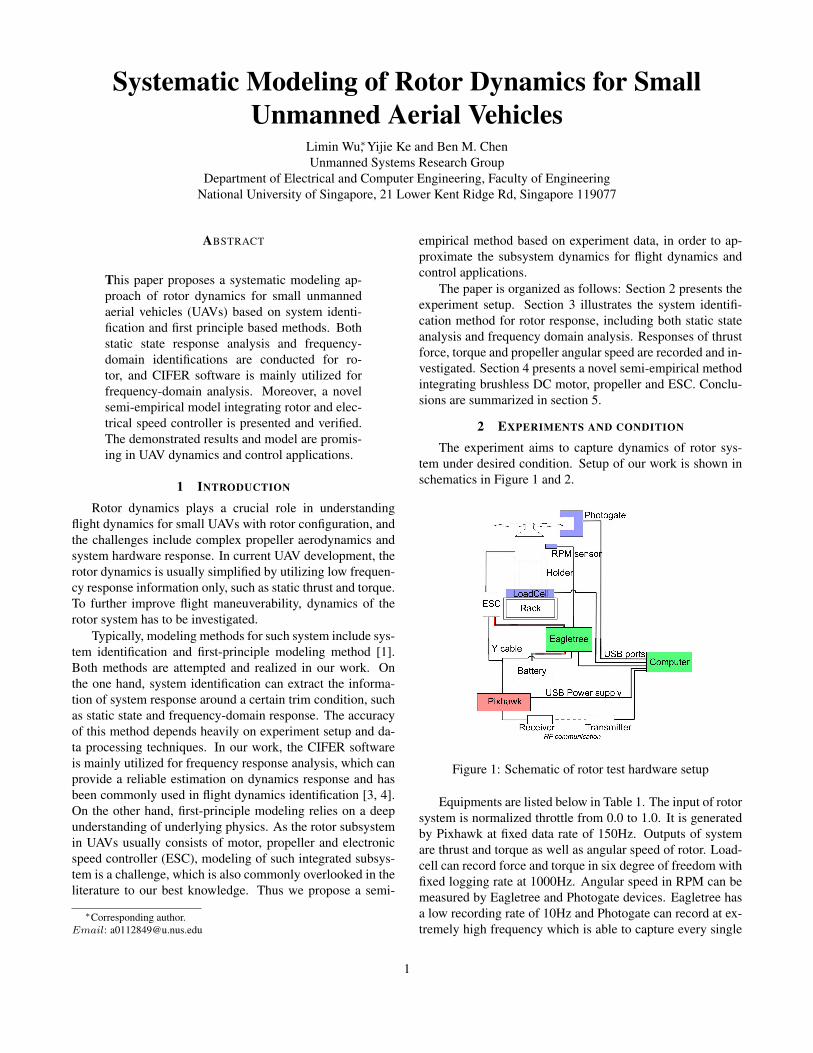
Figure 1: Schematic of rotor test hardware setup

Equipments are listed below in Table 1. The input of rotorsystem is normalized throttle from 0.0 to 1.0. It is generatedby Pixhawk at fixed data rate of 150Hz. Outputs of systemare thrust and torque as well as angular speed of rotor. Load-cell can record force and torque in six degree of freedom withfixed logging rate at 1000Hz. Angular speed in RPM can bemeasured by Eagletree and Photogate devices. Eagletree hasa low recording rate of 10Hz and Photogate can record at ex-tremely high frequency which is able to capture every single

1

Figure 2: Rotor test setup

Name DescriptionAPC 11X5.5P Propeller rotor propeller

Scorpion 3026 motor brushless DC motorScorpion Commander 90A ESC

4-cells LiPo battery power supplyoptical RPM sensor angular speed measuring device

Photogate angular speed measuring deviceATI load cell 6 DOF force and torque logging

Pixhawk PWM throttle input generatorEagleTree elogger V4 battery voltage and current recording

rack and holder supporting platformcomputer sensor data collection

Table 1: LIST OF EQUIPMENTS

revolution of rotor. Power is supplied by LiPo battery insteadof DC power supply because battery has limited dischargerate. And we want to study the dynamics of rotor with thesame discharge rate in power source as our actual UAVs.

3 SYSTEM IDENTIFICATION METHOD

Both static state analysis and frequency-domain identifi-cation methods are utilized for rotor dynamics based on ourexperiment setup. The static state response can help identi-fy step-response features for interested states, while frequen-cy response can extract richer dynamics information arounda trim condition. In this section, main results of these twomethods will be presented, and we are mainly concerned withthe propeller thrust, torque and angular speed.

3.1 Static state analysis3.1.1 Stimulus signal

Stimulus signal for static state analysis is shown in lower partof Figure 3, which includes 10 step functions with amplitudeincreased from 0.1 to 1.0 with step size 0.1. Duration of eachstep function is 5 seconds therefore total duration is 50 sec-onds.

3.1.2 Angular speed channel

Result from step signal test indicates the steady-state angularspeed when throttle varies from 0.1 to 1.0 with step size 0.1.Table 2 and Figure 3 show the result. As can be observed in

Throttle Steady-state Angular speed (rad/s)0.10 228.180.20 423.170.30 566.850.40 689.580.50 737.540.60 788.020.70 832.840.80 892.740.90 937.351.00 941.54

Table 2: RELATION BETWEEN THROTTLE ANDSTEADY-STATE ANGULAR SPEED

0

200

400

600

800

1000Angular speed (rad/s)

5 10 15 20 25 30 35 40 45 500

0.2

0.4

0.6

0.8

1Throttle

Input-Output Data

Time (seconds)

Am

plitu

de

Figure 3: Plot of measured angular speed with correspondingthrottle in step signal test

figure and table, angular speed changes proportional to throt-tle. The relation can be summarized as function:

ω = −1080u2 + 1952u+ 42(0 6 u 6 1) (1)

where ω is angular speed in rad/s and u is normalized throttle.

3.2 Frequency domain analysis

3.2.1 Stimulus signal

Stimulus signal for frequency domain analysis is selected tobe a sinusoidal wave swept from 0.05Hz to 20Hz at throttleequals to 0.6 equilibrium point. The frequency range is se-lected based on our flight control design as higher frequencyexceeds greatly the control bandwidth. However, in order toeliminate effect from battery voltage drop, this chirp signaltest has been divided into three experiments:

2

Time (seconds)0 5 10 15 20 25 30 35 40 45 50

Am

plitu

de

0.1

0.2

0.3

0.4

0.5

0.6

0.7

0.8Throttle

(a) Experiment 1Time (seconds)

0 5 10 15 20 25 30 35 40 45 50

Am

plitu

de

0.1

0.2

0.3

0.4

0.5

0.6

0.7

0.8Throttle

(b) Experiment 2

Time (seconds)0 5 10 15 20 25 30 35 40 45 50

Am

plitu

de

0.1

0.2

0.3

0.4

0.5

0.6

0.7Throttle

(c) Experiment 3

Figure 4: Chirp stimulus signal

• Experiment 1: Chirp signal swept from 0.05Hz to0.5Hz, test duration 50s includes 10s warm-up.

• Experiment 2: Chirp signal swept from 0.5Hz to 5Hz,test duration 50s includes 10s warm-up.

• Experiment 3: Chirp signal swept from 5Hz to 20Hz,test duration 50s includes 10s warm-up.

All three chirp signals have been plotted in Figure 4.

3.2.2 Thrust channel

Following figures show the relationship between throttle andthrust in both time domain (Figure 5, Figure 6 and Figure 7)and frequency domain (Figure 8), and this set of data is col-lected during the chirp signal rotor test. The first 10 secondswarm-up section and mean value will be removed by CIFERduring data preprocessing as the response near equilibrium isour interest.

-10

0

10

20Thrust force (N)

5 10 15 20 25 30 35 40 45 500

0.5

1Throttle

Input-Output Data

Time (seconds)

Am

plitu

de

Figure 5: Thrust channel, time domain data of experiment 1

The system in thrust channel has a decreasing gain withfrequency. The plot of coherence in Figure 8 indicates the ac-curacy of frequency estimation. For rotorcraft, recommended

-5

0

5

10

15Thrust force (N)

5 10 15 20 25 30 35 40 45 500

0.2

0.4

0.6

0.8Throttle

Input-Output Data

Time (seconds)

Am

plitu

de

Figure 6: Thrust channel, time domain data of experiment 2

-5

0

5

10

15ForceZ

5 10 15 20 25 30 35 40 45 500

0.2

0.4

0.6

0.8Throttle

Input-Output Data

Time (seconds)

Am

plitu

de

Figure 7: Thrust channel, time domain data of experiment 3

threshold coherence value is 0.6 according to [4]. Therefore,Figure 8 tells that the estimation is credible within the rangeof frequency up to 30 rad/s. Phase plot suggests that systemhave a -135 degree phase at 30 rad/s. Hence the system canbe approximated by a second order system within confidencerange. Then parameter identification is applied and identifi-cation result is:

8859

(s+ 9.35)(s+ 61.52)(2)

which DC gain = 15.40, Bandwidth = 9.12 rad/s.

Figure 8: Thrust channel, Bode plot estimated by CIFER

3

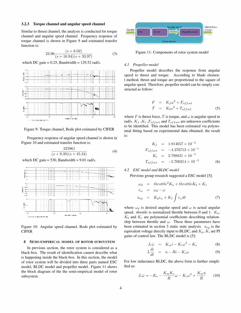
3.2.3 Torque channel and angular speed channel

Similar to thrust channel, the analysis is conducted for torquechannel and angular speed channel. Frequency response oftorque channel is shown in Figure 9 and estimated transferfunction is:

23.96(s+ 6.02)

(s+ 16.94)(s+ 33.97)(3)

which DC gain = 0.25, Bandwidth = 129.52 rad/s.

Figure 9: Torque channel, Bode plot estimated by CIFER

Frequency response of angular speed channel is shown inFigure 10 and estimated transfer function is:

225961

(s+ 9.39)(s+ 45.34)(4)

which DC gain = 530, Bandwidth = 9.01 rad/s.

Figure 10: Angular speed channel, Bode plot estimated byCIFER

4 SEMI-EMPIRICAL MODEL OF ROTOR SUBSYSTEM

In previous section, the rotor system is considered as ablack-box. The result of identification cannot describe whatis happening inside the black-box. In this section, the modelof rotor system will be divided into three parts named ESCmodel, BLDC model and propeller model. Figure 11 showsthe block diagram of the the semi-empirical model of rotorsubsystem.

Figure 11: Components of rotor system model

4.1 Propeller modelPropeller model describes the response from angular

speed to thrust and torque. According to blade elemen-t method, thrust and torque are proportional to the square ofangular speed. Therefore, propeller model can be simply con-structed as follow:

F = Kfω2 + Foffset

T = Ktω2 + Toffset (5)

where F is thrust force, T is torque, and ω is angular speed inrad/s. Kf ,Kt ,Foffset and Toffset are unknown coefficientsto be identified. This model has been estimated via polyno-mial fitting based on experimental data obtained, the resultis:

Kf = 1.814657× 10−5

Foffset = −4.376713× 10−1

Kt = 2.798821× 10−7

Toffset = −5.700314× 10−3 (6)

4.2 ESC model and BLDC modelPrevious group research suggested a ESC model [5]:

ωd = throttle2Ka + throttleKb +Kc

eω = ωd − ω

ueq = Kpeω +KI

∫eωdt (7)

where ωd is desired angular speed and ω is actual angularspeed. throttle is normalized throttle between 0 and 1. Ka,Kb and Kc are polynomial coefficients describing relation-ship between throttle and ω. These three parameters havebeen estimated in section 3 static state analysis. ueq is theequivalent voltage directly input to BLDC, andKp, Ki are PIgains of control law. The BLDC model is [5]:

Jrω = Kmi−Krω2 −Ks (8)

Ldi

dt= u−Ri−Keω (9)

For low inductance BLDC, the above form is further simpli-fied as:

Jrω = −Ks −KmKe

Rω −Krω

2 +Kmu

R(10)

4

where u is the input voltage, Jr is rotor inertia, Km, Ks andKe are motor electrical parameters, and R is the resistance.The output of ESC ueq is equivalent to u, input of BLDCmodel.

As only throttle input and angular speed ω are measur-able, a nonlinear model of above subsystem is derived as be-low with an augmented state xa:

ω = −Ks

Jr− KmKe

RJrω − Kr

Jrω2 + KmKi

RJrxa +

KpKm

RJrωd

xa = −ω + ωd (11)

where Ks,Km,Ke,Kp,Ki, R and Jr are parameters underidentification. All parameters are positive.

4.3 Model identification methodParameter identification is achieved by Matlab function

”nlgreyest”, which estimates the unknown nonlinear grey-box model parameters based on measured data. The functionemploys minimization schemes with embedded line search-ing methods for parameter estimation. Initial value and rangeof parameters are estimated according to first principle.

4.4 Estimation of parameter range• Effective motor resistanceR is effective Motor Resistance. It can be found in datasheet of motor.

• Rotor inertiaJr is the moment of inertia of propeller and rotor. Thisparameter can be estimated by considering them as athin rod rotating about its middle point. Correspondingformula to calculate Jr is:

Jr =mr2

12(12)

where m is mass of rod and r is radius of the thin rod.

• Equivalent drag coefficientKrω

2 represents reaction torque from propeller. There-fore, Kr is equivalent to drag coefficient Kf obtainedin section 4.1.

• Motor torque constantMotor Torque constantKm can be calculated by apply-ing following formula:

Km =60

2πKv(13)

where Kv is motor velocity constant given in motordata sheet.

• Back EMF constantBack EMF constant Ke. In the three phase BLDC mo-tors the relationship is approximately equal to [6]:

Ke =

√3

2Km (14)

• Static friction torque constantKs is static friction torque constant. It can be mea-sured by torque meter. It usually has much less effectto torque when compared with back EMF and reactiontorque of propeller. Hence, it is assumed that this termhas 2 order of magnitude smaller than Krω

2 term andKmKe

R ω term in equation (10).

• Proportional GainKp is proportional gain of control law. It can be es-timated by using instantaneous angular accelerationwhile rotor is changing from one trim condition to an-other. Formula used to estimated Kp is:

Jrω =Km

RKpeω (15)

where ω is angular acceleration and eω is differenceangular speed between two trim conditions.

• Integral GainKi represents integral gain of control law. It can be es-timated by observing the transition from one trim con-dition to another. equation (7) and equation (10) can beapplied to both trim conditions, thus following equa-tions can be obtained:

0 = −Ks

Jr− KmKe

RJrω1 −

Kr

Jrω1

2 +KmKi

RJr

∫eω1dt

(16)

0 = −Ks

Jr− KmKe

RJrω2 −

Kr

Jrω2

2 +KmKi

RJr

∫eω2dt

(17)

ω1 and ω2 are steady-state angular speed for two trimconditions respectively, and both values are measur-able. The difference between

∫(eω1dt) and

∫(eω2dt)

can be obtained by integrating eω over transition inter-val between two trim conditions. Therefore, Ki canbe estimated by minusing equation (17) with equation(16).

Based on estimated initial values, parameter ranges aredefined as shown in Table 3. For parameters calculated fromgiven value in datasheet, range is defined as ±10% of initialvalue. For parameters calculated from measured data in ex-periment, range is defined as ±50% of initial value.

4.5 Result and comparisonWith aforementioned parameter range and propeller mod-

el, Matlab function ”nlgreyest” is used to identify the param-eters, and the results are shown in Table 4.

Figure 12 and Figure 13 show a comparison between ωfrom identified semi-empirical model and measured value. Inorder to verify model fidelity, NRMSE fitness value is used inMatlab, as defined by

fit% = 100%(1− ‖p− p‖‖p−mean(p)‖

) (18)

5

Parameter Initial value RangeR 0.014 ±10%Jr 3× 10−5 ±50%Kr 2.8× 10−7 ±10%Km 0.01 ±10%Ke 0.012 ±10%Ks 10−2 ±50%Kp 2.6× 10−4 ±50%Ki 7× 10−2 ±50%

Table 3: RANGE OF PARAMETERS

Parameter ValueR 0.0154Jr 4.5× 10−5

Kr 3.08× 10−7

Km 0.009Ke 0.0132Ks 1.5× 10−2

Kp 1.3× 10−4

Ki 0.069

Table 4: IDENTIFIED PARAMETERS

where p is the validation data collected during experimen-t and p is the output generated by BLDC model. The 75.72%fitness shows that our model prediction fits well with real ex-periment data.

Another model validation standard is Theil inequalitycoecient[7] (TIC), which is defined by

TIC =

√1n

∑ni=1(p− p)2√

1n

∑ni=1(p)2 +

√1n

∑ni=1(p)2

(19)

where n is the total sample amount, p is the validation datacollected during experiment and p is the output generated byBLDC model. TIC is a normalized value between [0, 1], andzero indicates a perfect matching. In practice, the thresholdof TIC is commonly set at 0.25 [8]. As for TIC-based valida-tion, results for Experiment 1 and 2 are 0.020 and 0.025 re-spectively. Both TIC value are much lower than the thresholdvalue 0.25. Therefore, results indicate that identified BLDCmodel has sufficient accuracy.

After linearized at throttle = 0.6 trim condition, BLD-C model is combined with ESC and propeller models, thencompared with transfer function obtained through identifica-tion approach in section 3. Input is throttle and output is thrustforce. Bode plots are shown in Figure 14.

Bode plot of system identified from semi-empirical mod-el has a DC gain equals to 21.8dB and bandwidth 4.95 rad/s.For transfer function identified by CIFER, DC gain is 23.7d-B and bandwidth is 9.12 rad/s. The comparison (Figure 14)

Time (seconds)

Am

plitu

de

5 10 15 20 25 30 35 40 450

200

400

600

800

1000Time Response Comparison

Om

ega

(rad

/s)

Experimental dataBLDC model result

Time (seconds)

TIC = 0.020

Fit = 75.72%

Figure 12: BLDC model result compare with measured an-gular speed (Experiment 1)

Time (seconds)

Am

plitu

de

5 10 15 20 25 30 35 40 450

200

400

600

800

1000Time Response Comparison

Om

ega

(rad

/s)

Experimental dataBLDC model result

Time (seconds)

Fit = 69.08%

TIC = 0.025

Figure 13: BLDC model result compare with measured an-gular speed (Experiment 2)

shows that our semi-empirical model can fit well with CIFERidentification up to 10 rad/s, and the accuracy implies that ourmodel is capable of predicting rotor dynamics and can be in-tegrated in real-time UAV dynamics and control applications.

5 CONCLUSIONS

To conclude, this paper presents a systematic modelingapproach for rotor dynamics integrating brushless DC mo-tor, propeller and ESC. First, static state analysis is done toindicate the behavior under various steady states. Then, fre-quency responses of dynamics in various channels are suc-cessfully generated. Transfer function models are estimatedand proven to be reliable for up to 20 rad/s. Finally, a novelsemi-empirical model is presented and validated by experi-mental data. The model is proven to fit well with frequencyresponse results up to 10rad/s and is promising in real-timeimplementation for UAV dynamics and control.

REFERENCES

[1] B. M. Chen, T. H. Lee, K. Peng and V. Venkataramanan,Hard Disk Drive Servo Systems, 2nd ed. New York, NY:Springer, 2006.

6

Mag

nitu

de (

dB)

-50

0

50

CIFER

Semi-empirical model

10-1 100 101 102 103

Pha

se (

deg)

-180

-90

0

CIFER

Semi-empirical model

Bode Diagram

Frequency (rad/s)

Figure 14: Bode plots of systems estimated by CIFER and bySemi-empirical model. Thrust channel

[2] Ljung L, “Linear Model Identification,” in System identi-fication toolbox, South Natick, MA:The MathWorks Inc.,1988.

[3] Comprehensive Identification from Frequency ResponsesUsers Guide, UCSC, Santa cruz, CA, 2012.

[4] G. Cai, B. M. Chen, T. H. Lee. Unmanned rotorcraft sys-tems, New York, NY:Springer Science & Business Medi-a, 2011, pp. 90-94 .

[5] Yijie Ke, “An empirical model to rotor dynamics withbrushless DC motor,” Internal report in NUS unmannedsystem research group.

[6] General motor terminology, The Motor & Motion Asso-ciation, S. Dartmouth, MA, 2015.

[7] M. B. Tischler, R. K. Remple , Aircraft and rotorcraft sys-tem identification: Engineering methods with flight testexamples, VA:American Institute of Aeronautics and As-tronautics, 2006.

[8] G. Cai, T. Taha, J.Dias amd L. Seneviratne, “A frame-work of frequency-domain flight dynamics modeling formulti-rotor aerial vehicles,”. Journal of Aerospace Engi-neering, May. 2016.

7