A1131

System Noise-Figure Analysis for Modern Radio Receivers: Part 1, Calculations for a Cascaded Receiver By: Charles Razzell, Executive Director, Maxim Integrated

Introduction The general concept of noise figure is well understood and widely used by system and circuit designers

alike. In particular, it is used to convey noise-performance requirements by product definers and circuit designers and to predict the overall sensitivity of receiver systems.

The principle difficulty with noise-figure analysis arises when mixers are part of the signal chain. All real

mixers fold the RF spectrum around the local oscillator (LO) frequency, creating an output which contains the summation of the spectrum on both sides according to . In heterodyne architectures one of these

contributions may be considered spurious and the other intended. Therefore, image reject filtering or image canceling schemes are likely to be employed to largely remove one of these responses. In direct-conversion receivers, the case is different; both sidebands (above and below ) are converted and utilized for the

wanted signal. Consequently, this is truly a double-sideband application of the mixers. Various definitions commonly used in industry acount for noise folding to different degrees. For example,

the traditional single-sideband noise figure, assumes that the noise from both sidebands is allowed to fold into

the output signal, but only one of the sidebands is useful for conveying the wanted signal. This naturally results in a 3dB increase in noise figure, assuming that the conversion gain at both responses is equal. Conversely, the double-sideband noise figure assumes that both responses of the mixer contain parts of the wanted signal and, therefore, noise folding (along with corresponding signal folding) does not impact the noise figure. The double-sideband noise figure finds application in direct-conversion receivers as well as in radio astronomy receivers. However, deeper analysis will show that it is not sufficient for designers just to choose the right “flavor” of noise figure for a given application and then to substitute the corresponding number into the standard Friis equation. Doing

so can lead to substantially faulty analysis, which may be particularly severe in cases when the mixers or components following the mixer play a non-negligible role in determining system noise figure.

This article ties together the fundamenal definition of noise figure, equation-based analysis of cascade

blocks involving mixers, and typical lab techniques for measuring noise figure. In this Part 1 we show how the cascaded noise figure equation is modified by the presence of one or mixers and we derive the applicable equations for a number of popular downconversion architectures. We continue this discussion in Part 2 of this series where we describe the Y-factor method of noise-figure measurement. In Part 2 we focus on the case of a mixer as the device under test in order to identify appropriate measurement methods for mixer noise figures that can be validly applied using the cascade equations derived in Part 1.

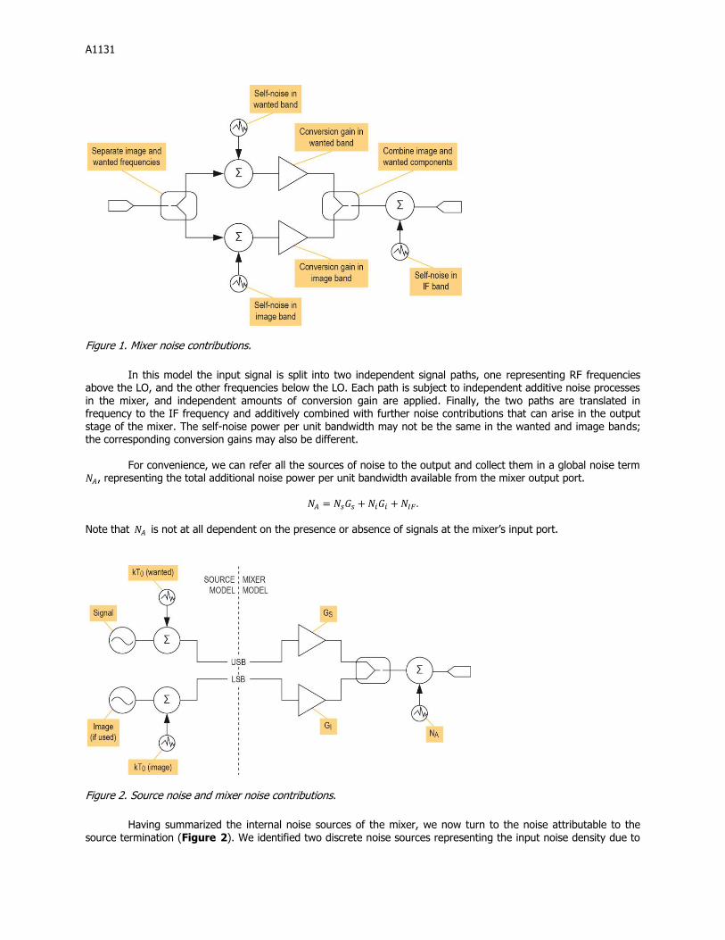
Conceptual Model of Mixer Noise One way to visualize mixer noise contributions is to consider a conceptual model of a mixer (Figure 1). This

model is based on one1 provided by Agilent’s Genesys Simulation Program.

A1131

Figure 1. Mixer noise contributions.

In this model the input signal is split into two independent signal paths, one representing RF frequencies

above the LO, and the other frequencies below the LO. Each path is subject to independent additive noise processes in the mixer, and independent amounts of conversion gain are applied. Finally, the two paths are translated in frequency to the IF frequency and additively combined with further noise contributions that can arise in the output stage of the mixer. The self-noise power per unit bandwidth may not be the same in the wanted and image bands; the corresponding conversion gains may also be different.

For convenience, we can refer all the sources of noise to the output and collect them in a global noise term

, representing the total additional noise power per unit bandwidth available from the mixer output port.

Note that is not at all dependent on the presence or absence of signals at the mixer’s input port.

Figure 2. Source noise and mixer noise contributions.

Having summarized the internal noise sources of the mixer, we now turn to the noise attributable to the

source termination (Figure 2). We identified two discrete noise sources representing the input noise density due to

A1131

the source termination at the wanted frequency and the image frequency, respectively. We must account for these

as independent quantities, because the application circuit can cause one of them to be attenuated and the other transferred with low loss into the mixer’s RF input port. This will likely be the case, if the image and wanted RF frequencies are well separated and a frequency-selective match is employed.

In the case of a broadband match we could write, . However, in the case of a

high-Q, frequency selective match to the mixer at the wanted RF frequency, the noise at the output due to the source termination at the image frequency may be negligible, leading to . Generally, we can

assign a coefficient, , to the effective fraction of the input source-termination noise power available to the mixer’s input port at the image frequency. Thus, , where is an application-specific coefficient

in the range . Later we shall see that the effective noise figure in an application depends on the value of .

Noise-Figure Definitions Before discussing why cascaded noise-figure calculations can be misleading, we should review some basic

definitions of the term. A reasonable starting point for explaining noise factor for a two-port network is:

Which, when expressed in dB, is termed the noise figure :

This expression depends on the SNR of the input signal. If SNR is left undefined, however, this measure is meaningless as a performance measure of the circuit or component itself, since it largely depends on the quality of the signal feeding it. Therefore, it is desriable to take the best-case assumption for the SNR at the input, namely that the only source of noise is due to the thermal noise of the input termination, at some defined temperature. It is also logical to assume that the noise factor does not depend on the signal levels used. This assumes that the two-port network being characterized is in its linear operating region. This can be seen if we let the input signal power be

and the signal gain be . Then, the output power is given by and:

Furthermore, these noise powers, and are ill-defined unless we specify the bandwidths in which they are

measured. This can be solved by specifying and to represent noise power per unit bandwidth at any given

specified input frequency.

Single Sideband Noise Factor The above considerations help to explain the rationale for the IEEE® definition of Noise Factor:

Noise Factor (of a Two-Port Transducer). At a specified input frequency the ratio of 1) the total noise power per unit bandwidth at a corresponding output frequency available at the output Port to 2) that portion of 1) engendered at the input frequency by the input termination at the Standard Noise Temperature (290 K). For heterodyne systems there will be, in principle, more than one output frequency corresponding to a single input frequency, and vice versa; for each pair of corresponding frequencies a Noise Factor is defined. The phrase “available at the output Port" may be replaced by “delivered by the system to an output termination." To characterize a system by a Noise Factor is meaningful only when the admittance (or impedance) of the input termination is specified.2

This definition of noise factor is a point function of output frequency, with respect to one corresponding RF frequency (not a pair of RF frequencies simultaneously, which is what makes it a single sideband noise factor; see Figure 3).

A1131

Figure 3. SSB noise figure.

It is important to note that the denominator only includes noise from one sideband; the numerator

comprises the total noise power per unit bandwidth at a corresponding output frequency without making any specific exclusions. To make this explicit in mathematical form for the case of a mixer with signal and image responses, the above definition can be written as:

Where is the conversion gain at the image frequency; is the conversion gain at the signal frequency; is the

standard noise temperature; and is the noise power per unit bandwidth added by the mixer’s electronics as

measured at the output terminals. The corresponding noise factor for the image frequency can be written as:

This will be a different number if the conversion gain at the image frequency is different to that at the wanted signal frequency. There are some3 who interpret the IEEE definition above to exclude the image noise from the term “total noise power per unit bandwidth at the corresponding output frequency available at the output Port.” They therefore assume:

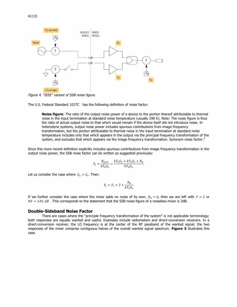
This definition corresponds to a situation where the source input noise at the image frequency is fully excluded from the mixer’s input port. This interpretation is not widely utilized by industry practitioners. Nevertheless, for the sake of completeness, it is illustrated in Figure 4.

A1131

Figure 4. “IEEE” variant of SSB noise figure.

The U.S. Federal Standard 1037C has the following definition of noise factor:

Noise figure: The ratio of the output noise power of a device to the portion thereof attributable to thermal noise in the input termination at standard noise temperature (usually 290 K). Note: The noise figure is thus the ratio of actual output noise to that which would remain if the device itself did not introduce noise. In heterodyne systems, output noise power includes spurious contributions from image-frequency transformation, but the portion attributable to thermal noise in the input termination at standard noise temperature includes only that which appears in the output via the principal frequency transformation of the system, and excludes that which appears via the image frequency transformation. Synonym noise factor.4

Since this more recent definition explicitly includes spurious contributions from image frequency transformation in the output noise power, the SSB noise factor can be written as suggested previously:

Let us consider the case where . Then:

If we further consider the case where the mixer adds no noise of its own, , then we are left with or

.This corresponds to the statement that the SSB noise figure of a noiseless mixer is 3dB.

Double-Sideband Noise Factor There are cases where the “principle frequency transformation of the system” is not applicable terminology;

both responses are equally wanted and useful. Examples include radiometers and direct-conversion receivers. In a direct-conversion receiver, the LO frequency is at the center of the RF passband of the wanted signal; the two responses of the mixer comprise contiguous halves of the overall wanted signal spectrum. Figure 5 illustrates this case.

A1131

Figure 5. DSB noise figure.

Therefore, in such cases it makes sense to consider a double-sideband noise factor:

If we assume that , then:

Under the same constraint:

This leads to the observation that, where both conversion gains are equal, the SSB noise figure of the mixer will be 3dB higher than the corresponding DSB noise figure. Moreover, if the mixer does not add any additional noise ( ), then or

Use of Noise Figures in Cascaded System Noise-Figure Calculations

Baseline Case: Cascade of Linear Circuit Blocks Consider the following simple cascade of three amplifier blocks (Figure 6).

Figure 6. Three gain blocks cascaded.

The total noise at the output can be calculated as:

A1131

The noise at the output that is attributable to the thermal noise at the input of the cascade is:

This implies that the overall noise factor is:

Substituting:

Yields:

This can be recognized as the standard Friis cascaded noise equation for three blocks. Extension to any number of blocks is trivial from here.

A Heterodyne Conversion Stage Consider the following frequency conversion stage in a receiver signal path (Figure 7). The

double-sideband noise figure of the mixer is 3dB and its conversion gain is 10dB. The wanted carrier frequency is at

2000MHz and the LO is chosen at 1998MHz, so that both the wanted and image frequencies are within the passband of the of the filter.

Figure 7. Heterodyne stage with no image rejection.

The cascaded performance of this arrangement is summarized in Table 1, where CF is the channel

frequency; CNP is the channel noise power; GAIN is the stage gain; CGAIN is the cascaded gain upto and including the present stage; and CNF is the cascaded noise figure.

Table 1. Simulated Casacaded Performance*

A1131

Parts CF (MHz) CNP (dBm) GAIN (dB) CGAIN (dB) CNF (dB)

CWSource_1 2000 -113.975 0 0 0

BPF_Butter_1 2000 -113.975 -7.12E-04 -7.12E-04 6.95E-04

BasicMixer_1 2 -97.965 10 9.999 6.011

* No image rejection from filter.

The overall cascaded gain of these two blocks is 9.999dB, while the SSB noise figure is 6.011dB. This noise

figure could have been correctly anticipated from the previous analyis, since we expect the SSB noise figure to be 3.01dB higher than the DSB figure of the mixer. There is an additional, very small noise figure degradation due to the finite insertion loss of the filter. Overall, this result meets our expectations.

Now we consider the same scenario, but with the LO frequency returned to 1750MHz (Figure 8). At this

value of the LO frequency, the image is at 1500MHz which is well outside the passband of the filter in front of the mixer.

Figure 8. Heterodyne stage with image rejection.

The cascaded performance of this arrangement is summarized in Table 2. The gain of the wanted signal is

the same as before, but the cascaded noise figure (CNF) has altered to a value of 4.758dB.

Table 2. Simulated Casacaded Performance* Parts CF (MHz) CNP (dBm) GAIN (dB) CGAIN (dB) CNF (dB)

CWSource_1 2000 -113.975 0 0 0

BPF_Butter_1 2000 -113.975 -7.12E-04 -7.12E-04 6.95E-04

BasicMixer_1 250 -99.218 10 9.999 4.758

* Significant image rejection from filter.

To explain this result, we need to consider that the noise situation in this scenario is similar to that depicted

in Figure 4. Specifically, the source impedance image noise is suppressed. The added noise from the mixer stage can be calculated from the previously derived equation for the DSB noise factor:

Therefore:

Now the total noise at the output of the mixer is given by with in this

application. Thus:

A1131

The resulting noise figure can be written as:

Expressing this in dB, we have:

This should be compared to the simulated value of 4.758dB, which included a tiny additional contribution from the insertion loss of the filter.

In general, the effective single sideband noise figure for the mixer stage is given by:

Where for the case where termination noise at the image frequency is well suppressed, and where it is

not suppressed at all. Note that if , the effective SSB noise figure reduces to which is the case

illustrated at the beginning of this section. In some scenarios, fractional values of can arise, e.g., if the image

suppression filter is not directly coupled to the mixer input terminals or if the frequency separation between image and wanted responses is not large.

A Heterodyne Receiver We can see how to apply the effective noise figure in larger cascade analysis with the example in Figure 9.

To calculate the cascaded noise figure of the entire chain, we need to encapsulate the mixer and its associated LO and image reject filtering as an equivalent two-port network that has specific gain and noise figure. The effective noise factor of this two-port network is since the termination noise at the image frequency

is well suppressed by the preceeding filter.

Figure 9. Heterodyne mixer in the context of adjacent system blocks.

Note that the applicable noise figure is neither the DSB nor the SSB noise figure of the mixer. Instead it is

an effective noise figure that lies somewhere between these two values. In this case with a DSB noise figure of 3dB, the equivalent noise figure of the two-port network can be calculated to be 4.757dB, as already noted above. Using this value in the overall cascade calculation results in a system noise figure of 7.281dB, as shown in Table 3. Manual calculations show that this result is consistent with the standard Friis equation using 4.757dB for the mixer noise figure.

Table 3. Simulated Cascade Performance of Heterodyne Mixer in a System

Parts CF (MHz) CNP (dBm) GAIN (dB) SNF (dB) CGAIN (dB) CNF (dB)

A1131

CWSource_1 2000 -113.975 0 0 0 0

Lin_1 2000 -100.975 10 3 10 3

BPF_Butter_1 2000 -100.976 -7.12E-04 7.12E-04 9.999 3

BasicMixer_1 250 -90.563 10 3 19.999 3.413

Lin_2 250 -61.695 25 25 44.999 7.281

In general, when subsituting an equivalent two-port network for the mixer and its adjacent components, the

input port should be the latest node in the signal flow for which the image response is rejected. The output port should be the earliest node where the image and wanted responses are combined together (usually the output port of the mixer). If the image response of the mixer is not effectively suppressed by the architecture, then the Friis equation cannot be used without modification.

A Zero-IF Receiver Now consider a zero-IF, or direct-conversion receiver (Figure 10).

Figure 10. ZIF receiver with LNA, mixers, filters and VGAs. This lineup consists of an LNA with 10dB of gain and 3dB noise figure; a bandpass filter centered at

950MHz; a signal splitter to send the signal to a pair of mixers, each with a conversion gain of 6dB; and a DSB noise figure of 4dB. The VGAs are defined to have gain of 10dB and a 25dB noise figure. A simulation of this lineup produced the results shown in Table 4.

Table 4. ZIF Receiver Lineup*

Parts CF (MHz)

CP (dBm)

CNP (dBm)

GAIN (dB)

SNF (dB)

CGAIN (dB)

CNF (dB)

MultiSource_1 950 -79.999 -116.194 0 0 0 0

FE_BPF 950 -80.009 -116.194 -9.99E-03 1.00E-02 -9.99E-03 9.99E-03

Lin_1 950 -70.008 -103.194 10 3 9.99 3.01

Split2_1 950 -73.018 -105.992 -3.01 3.01 6.98 3.222

BasicMixer_1 0 -67.039 -99.425 5.979 4 12.959 3.81

LPF1 0 -67.04 -99.425 -8.23E-04 1.00E-02 12.958 3.81

Lin_2 0 -57.036 -83.078 9.995 25 22.953 10.163

LPF2 0 -57.038 -83.08 -1.90E-03 1.00E-02 22.951 10.163

A1131

*The items tabulated are channel frequency (CF), channel power (CP), stage gain (GAIN), stage noise figure (SNF),

casacded gain (CGAIN), and cascaded noise figure (CNF).

Now in Table 5 we compare this result to an Excel® spreadsheet calculation using the Friis formula for

cascaded noise figure.

Table 5. Friis Cascade Equation Results

Parts F (dB) Gain (dB) CGAIN (dB) CNF (dB)

BPF filter 0.01 -0.01 -0.01 0.01

LNA 3 10 9.99 3.01

Splitter 3.01 -3.01 6.98 3.22

Mixer 4 5.979 12.96 3.81

LPF1 0.01 -0.01 12.95 3.81

VGA 25 9.995 22.94 12.65

LPF2 0.01 -0.01 22.93 12.65

Clearly something has gone wrong with the cascaded noise figure. We are estimating 12.64dB using the

spreadsheet, but the simulator is finding 10.16dB. The cascaded gains match reasonably well, but we need to establish which of the noise figures is valid. First, we are interested in the double-sideband noise figure of the entire structure, since the entire ZIF structure will use signals in both sidebands and suffer noise in both sidebands. Therefore, it is relevant to derive the double-sideband noise figure of a cascade involving an amplifier, followed by a mixer, followed by an additional amplifier (Figure 11).

Figure 11. Cascade including a mixer.

The total noise density at the output can be calculated as:

The noise at the output that is attributable to the thermal noise at the input of the cascade is:

This implies that the overall noise factor is:

G

Substituting:

Yields:

A1131

This derivation indicates that it is necessary to use the DSB noise figure of the mixer in the cascade equation, and that the noise contributions from all following stages must be divided by 2 with respect to the usual form of the Friis equation for a cascaded noise figure. The failure to perform this latter division by 2 caused the spreadsheet equation analysis shown in Table 5 to be wrong. Amending the equations in the spreadsheet cells after the mixer to include the necessary division by 2 gives the result shown in Table 6.

Table 6. DSB Cascade Equation Results

Parts F (dB) Gain (dB) CGAIN (dB) CNF (dB)

BPF filter 0.01 -0.01 -0.01 0.01

LNA 3 10 9.99 3.01

Splitter 3.01 -3.01 6.98 3.22

Mixer 4 5.979 12.96 3.81

LPF1 0.01 -0.01 12.95 3.81

VGA 25 9.995 22.94 10.17

LPF2 0.01 -0.01 22.93 10.17

The agreement between Table 6 and Table 4 is now good. However, this exercise has also demonstrated

the dangers of directly substituting into the Friis cascade equation where mixers are involved.

Now we consider the same scenario, but with the wanted signal 300kHz higher than the LO. The block

diagram remains as illustrated in Figure 10, but all of the signal falls on the high side of the LO. This makes it a low-IF (LIF) application of the same receiver architecture. Using the same Genesys simulation workspace as before, the results are as shown below in Table 7.

Table 7. LIF Receiver Simulation Results

Parts CF (MHz)

CP (dBm)

CNP (dBm)

GAIN (dB)

SNF (dB)

CGAIN (dB)

CNF (dB)

MultiSource_1 950.3 -79.999 -116.194 0 0 0 0

FE_BPF 950.3 -80.009 -116.194 -9.99E-03 1.00E-02 -9.99E-03 9.99E-03

Lin_1 950.3 -70.008 -103.194 10 3 9.99 3.01

Split2_1 950.3 -73.018 -105.992 -3.01 3.01 6.98 3.222

BasicMixer_1 0.3 -67.067 -96.335 5.938 4 12.918 6.94

LPF1 0.3 -68.467 -96.458 -1.64E-03 1.00E-02 12.916 6.819

Lin_2 0.3 -58.832 -80.068 9.969 25 22.885 13.241

LPF2 0.3 -58.483 -80.072 -4.68E-03 1.00E-02 22.88 13.241

These results are similar to the previous simulation of the same architecture, except that the noise figure

has increased by 3dB. In fact, even if all the components of this system were noiseless, except the source resistance,

the noise figure would be 3dB. Essentially, this is an SSB application of the complex receiver structure and there are no measures to suppress the unwanted sideband. The derivation for the cascaded noise figure is identical to that already given, except that the output noise attributable to the thermal noise at the input of the cascade is once again:

So now:

A1131

Substituting:

Yields:

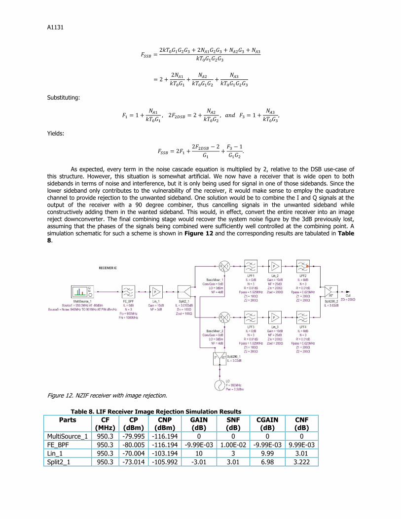
As expected, every term in the noise cascade equation is multiplied by 2, relative to the DSB use-case of this structure. However, this situation is somewhat artificial. We now have a receiver that is wide open to both sidebands in terms of noise and interference, but it is only being used for signal in one of those sidebands. Since the lower sideband only contributes to the vulnerability of the receiver, it would make sense to employ the quadrature channel to provide rejection to the unwanted sideband. One solution would be to combine the I and Q signals at the output of the receiver with a 90 degree combiner, thus cancelling signals in the unwanted sideband while constructively adding them in the wanted sideband. This would, in effect, convert the entire receiver into an image reject downconverter. The final combining stage would recover the system noise figure by the 3dB previously lost, assuming that the phases of the signals being combined were sufficiently well controlled at the combining point. A simulation schematic for such a scheme is shown in Figure 12 and the corresponding results are tabulated in Table 8.

Figure 12. NZIF receiver with image rejection. Table 8. LIF Receiver Image Rejection Simulation Results

Parts CF (MHz)

CP (dBm)

CNP (dBm)

GAIN (dB)

SNF (dB)

CGAIN (dB)

CNF (dB)

MultiSource_1 950.3 -79.995 -116.194 0 0 0 0

FE_BPF 950.3 -80.005 -116.194 -9.99E-03 1.00E-02 -9.99E-03 9.99E-03

Lin_1 950.3 -70.004 -103.194 10 3 9.99 3.01

Split2_1 950.3 -73.014 -105.992 -3.01 3.01 6.98 3.222

A1131

BasicMixer_1 0.3 -67.053 -96.441 5.958 4 12.938 6.815

LPF1 0.3 -67.055 -96.443 -1.64E-03 1.00E-02 12.936 6.815

Lin_2 0.3 -57.047 -80.09 9.991 25 22.927 13.177

LPF2 0.3 -57.051 -80.094 -3.82E-03 1.00E-02 22.923 13.177

Split290_2 0.3 -54.062 -80.145 3.001 3.02 25.923 10.125

The impovement of the cascaded noise figure (CNF) by 3dB at the final (combining) stage shows the

restoration of the noise figure, as expected.

Summary of Noise-Figure Calculations for a Cascaded Receiver We have seen that where a mixer is part of a receiver cascade, the Friis equation for cascaded noise factor

is not usually valid using either the DSB or SSB versions of the mixer noise figure. In cases where a filter is used to largely remove the image response of the receiver, an equivalent two-port network can be substituted for the mixer, filter, and LO subsystem. However, the resultant noise figure must be calculated from the DSB noise figure, taking account of the frequency selectivity of the source termination coupled to the mixer’s input port.

We have also found that the same physical structure can have a different effective noise figure, depending

on whether the signal is distributed around the LO or is entirely on one side of it (i.e., the application is DSB or SSB respectively). The 3dB loss in SNR caused by using a complex receiver in a low-IF (LIF) mode can be (and usually is) receovered by appropriate use of image reject combining, complex filtering, or equivalent baseband processing.

The use of Agilent® Genesys to simulate these architectures and scenarios has proven to agree with

mathematical derivations of the appropriate cascaded noise figure in the cases examined.

For each architecture discussed and simulated in this section, the cascaded noise factor equation is

summarized in Table 9.

Table 9. Summary of Derived Equations

Structure Application Cascaded F Equation

Three Gain

Blocks

Any

Heterodyne Mixer

SSB, ideal image filtering

Complex

Downconverter

ZIF

Complex Downconverter

LIF, no image suppression

Complex

Downconverter

LIF, image reject

combining

References 1 “Mixer Thermal Noise Figure,” Agilent Genesys Documentation, http://edocs.soco.agilent.com/display/genesys2010/MIXER_BASIC. 2 “IRE Standards on Electron Tubes: Definitions of Terms, 1957,” Proceedings of the IRE, vol. 45, pp. 983 –1010, July 1957. URL: http://ieeexplore.ieee.org/stamp/stamp.jsp?tp=&arnumber=4056638&isnumber=4056624 3 Maas, S., Microwave Mixers., Artech House Microwave Library, Artech House, 1993. 4 “Telecommunications: Glossary of Telecommunication Terms,” Federal Standard 1037C, http://www.its.bldrdoc.gov/fs-1037/fs-1037c.htm .

A1131

Agilent is a registered trademark and registered service mark of Agilent Technologies, Inc. Excel is a registered trademark of Microsoft Corporation. IEEE is a registered service mark of the Institute of Electrical and Electronics Engineers, Inc.

About the Author: Charles Razzell received his undergraduate electronics engineering degree from the University of Manchester Institute of Science and Technology (UMIST), U.K.. Since then, he has been involved in development and advanced development projects, usually with a focus on highly integrated transceiver designs. During the 1980s his technical work was mainly in the analog and RF design fields, including the design and layout of one of the earliest fully-integrated paging receiver ICs for Philips. His involvement in digital radio technology began in the early 1990s with TErrestrial Trunked Radio (TETRA), where he was involved in making a system proposal on behalf of Philips and made further contributions to the Physical Layer specification of that ETSI standard. At Maxim Integrated he is an Executive Director with responsibility for product definition, applications and product engineering. He has eighteen granted U.S. patents.