system modeling, analysis, and optimization methodology...
TRANSCRIPT
System Modeling, Analysis, and Optimization Methodology for Diesel Exhaust After-treatment Technologies
by
Christopher Dominic Graff
S.B. Aeronautics and Astronautics, 2004 Massachusetts Institute of Technology
Submitted to the Department of Aeronautics and Astronautics in partial fulfillment of the requirements for the degree of
Master of Science in Aeronautics and Astronautics
at the
MASSACHUSETTS INSTITUTE OF TECHNOLOGY
June 2006
© 2006 Massachusetts Institute of Technology. All rights Reserved.
Author ……………………………………………………………………………………...............
Department of Aeronautics and Astronautics May 22, 2006
Certified by………………………………………………………………………………................
Olivier L. de Weck Assistant Professor of Aeronautics and Astronautics and Engineering Systems
Thesis Supervisor
Accepted by………………………………………………………………………………............... Jaime Peraire
Professor of Aeronautics and Astronautics Chair, Committee on Graduate Students

2
System Modeling, Analysis, and Optimization Methodology for Diesel Exhaust After-treatment Technologies
by Christopher D. Graff
Submitted to the Department of Aeronautics and Astronautics
on 1 May 2006, in partial fulfillment of the requirements for the degree of
Master of Science in Aeronautics and Astronautics
Abstract Developing new aftertreatment technologies to meet emission regulations for diesel engines is a growing problem for many automotive companies and suppliers. Balancing manufacturing cost, meeting emission performance, developing competitive engine power, reducing weight and operational costs are all tradeoffs that companies and operators have to resolve for new aftertreatment technologies. However, no single technology has been able to address the wide range of performance and cost objectives in this field. The traditional design philosophy of developing components, optimizing them for particular operation states, and then adding them together into a system may not yield the best solution to this complex problem. Manufacturers may not be able to offer the best balance of performance and cost developing systems in this manner. Two useful product development tools that can address this issue is Systems Architecture and multidisciplinary design optimization (MDO). This thesis develops and exercises a framework for modeling, designing, analyzing, and optimizing of complex diesel exhaust after-treatment systems. The methodology presented addresses the issue of complexity of systems and their components, and how to use systems architecture to develop a modeling technique that allows for flexibility in design, coding and analysis. The framework also addresses the analysis of exhaust system models, and utilizes multidisciplinary system design optimization to improve the design of exhaust systems. It also shows how using a system design and optimization methodology can yield better system designs than the more traditional design and development method that addresses only one technological component at a time. Two case studies are presented to validate the framework and methodology, and a set of design solutions for each case are found. A modeling and simulation tool was also developed for this thesis, and presented. The valuable information gleaned from this analysis can assist engineers and designers in identifying design directions and developing complete diesel emissions treatment solutions. Thesis Supervisor: Olivier L. de Weck Title: Assistant Professor of Aeronautics and Astronautics and Engineering Systems
3

Blank Page
4

Acknowledgements
First, I would like to thank the Department of Aeronautics and Astronautics at MIT for their support and encouragement. The professors, staff, and students in the department were and are loyal, caring, and supportive of each and everyone, and offered unique challenges and support throughout my undergraduate and graduate education.
Second, I wish to thank my advisor, Olivier de Weck, for believing in me, and hiring me as a
research assistant in the graduate program. His support has been invaluable to my education, academic progress, and professional development. Prof. De Weck has helped me as a teaching assistant for one of his courses, has offered me opportunities outside the normal realm of academic research, and has been one of the biggest contributors to my development and success at MIT. Even with his busy schedule, he has been understanding and supportive at every opportunity, and has been more than just a mentor or advisor, in every sense of the word. He has truly been an inspiration.
Third, I would like to thank Rudy Smaling, and ArvinMeritor, Inc, who offered me the
opportunity and funding to perform the research for this thesis. And, thanks to everyone who I have had the opportunity and pleasure to meet at MIT and through Prof. de Weck: Bill Simmons, Gergana Bounova, Eun Suk Suh, and the rest of the de Weck Research Group.
And finally, I would like to thank my parents, family, Elina Tzatzalos, and friends for their
support and love throughout my undergraduate and graduate time at MIT, through good times and bad, and for always believing, supporting, and trusting in me. I love you!
5

Blank Page (page 6)
6
Contents Chapter 1 Introduction........................................................................................................................... 19
1.1 Motivation ................................................................................................................................. 19 1.1.1 Current State of Automotive Emission Regulations .............................................................. 20 1.1.2 Design and Development Motivation .................................................................................... 22 1.1.3 The basis behind MSDO and System Analysis ..................................................................... 23 1.1.4 Modeling and Simulation Needs for Diesel Exhaust Systems............................................... 30
1.2 Multidisciplinary Analysis and Design Optimization ............................................................... 32 1.2.1 MSDO and Optimization Methodology................................................................................. 32 1.2.2 Thesis Objectives and Goals .................................................................................................. 34
Chapter 2 Literature Review ................................................................................................................. 36
2.1 Current Technologies ................................................................................................................ 36 2.2 Future Technologies .................................................................................................................. 37 2.3 Modeling Research .................................................................................................................... 37
Chapter 3 Approach and Framework................................................................................................... 38
3.1 Modeling Architecture – Notional Framework ......................................................................... 39 3.2 State Vector Platform Concept – State Vector as Interface....................................................... 40
3.2.1 Operating State Vector Model ............................................................................................... 42 3.2.2 Component Modularity.......................................................................................................... 43 3.2.3 Modeling Framework and Implementation............................................................................ 44 3.2.4 Design and Parameter Inputs ................................................................................................. 45
3.3 Optimization Approach ............................................................................................................. 47 3.3.1 Framework Flow Chart and Optimization Implementation ................................................... 47 3.3.2 Algorithm Choice................................................................................................................... 48
Chapter 4 Model Components ............................................................................................................... 50
4.1 Diesel Oxidation Catalyst (DOC).............................................................................................. 50 4.2 Diesel Particulate Filter (DPF) .................................................................................................. 54
4.2.1 Filtration Sub-Model.............................................................................................................. 54 4.2.2 Pressure Drop Sub-Model...................................................................................................... 56 4.2.3 Mass and Energy Balance...................................................................................................... 56
4.3 Dosing System........................................................................................................................... 57 4.4 Heater/Combustor System......................................................................................................... 58 4.5 Lean NOx Trap (LNT) .............................................................................................................. 58
Chapter 5 Single Component Sizing Optimization: DOC Case Example.......................................... 63
5.1 Introduction ............................................................................................................................... 63 5.2 Design and Performance Objectives.......................................................................................... 64 5.3 Design Variables ....................................................................................................................... 65
5.3.1 DOC Design Vector............................................................................................................... 66 5.4 Design Constraints..................................................................................................................... 67 5.5 Simulation Parameters and Validation and Optimization Set-up .............................................. 67 5.6 Design Space Results for Single Objective Optimization using Gradient Based Algorithm .... 68
7
5.7 Transient and Steady State Design of Experiment Simulation for Different Oxidation Catalyst Formulations........................................................................................................................................... 72 5.8 Heuristic Algorithm Results for Single Objective Optimization............................................... 76 5.9 Design Space Results for Multi-objective Optimization ........................................................... 77 5.10 Computational Effort................................................................................................................. 87 5.11 Conclusions of the DOC Case Study......................................................................................... 87
Chapter 6 Multi-Objective and Multi-component Optimization: DOC/DPF Case Study ............... 89
6.1 Modeling Assumptions and Motivation .................................................................................... 90 6.2 Validation of Passive Regeneration........................................................................................... 92 6.3 Design Variables and Constraints............................................................................................ 105 6.4 Simulation Parameters............................................................................................................. 107 6.5 Objectives ................................................................................................................................ 108
6.5.1 Performance Objectives: ...................................................................................................... 108 6.5.2 Regeneration Objectives: ..................................................................................................... 109 6.5.3 Cost Objectives: ................................................................................................................... 109 6.5.4 Objectives Used During Optimization Routine ................................................................... 110
6.6 Initial Design Points and Architecture Comparison ................................................................ 110 6.6.1 Initial Passive System .......................................................................................................... 110 6.6.2 Initial Dosing System........................................................................................................... 112 6.6.3 Initial Heater System 1......................................................................................................... 113 6.6.4 Initial Heater System 2......................................................................................................... 114
6.7 Coarse Objective Space Results and Architectural Comparisons ........................................... 115 6.7.1 Genetic Algorithm Design Clouds in Objective Space........................................................ 116 6.7.2 Dosing System Pareto Fronts in Objective Space................................................................ 119 6.7.3 Heater 1 System Pareto Fronts in Objective Space.............................................................. 123 6.7.4 Heater 2 System Pareto Fronts in Objective Space.............................................................. 125 6.7.5 Comparison of Objective Space Tradeoffs Between System Architectures ........................ 127 6.7.6 Mapping Feasible Objective Space Results Back to Design Families................................. 129 6.7.7 Comparing Aspect Ratios between DOCs and DPFs .......................................................... 131
6.8 Objective Space Refinement Results....................................................................................... 134 6.9 Comparison With Individual Optimization ............................................................................. 138 6.10 Computational Effort............................................................................................................... 143 6.11 Summary.................................................................................................................................. 144
Chapter 7 Conclusions.......................................................................................................................... 145
7.1 Validation of Methodology and Approach.............................................................................. 145 7.2 Modularity and Flexibility....................................................................................................... 146
7.2.1 Future Changes .................................................................................................................... 146 7.2.2 Cost and Time Savings ........................................................................................................ 147
7.3 Case Study Conclusions .......................................................................................................... 150 7.4 Future Work............................................................................................................................. 151
Appendix A Model Component Details and Code .............................................................................. 157
A.1 Diesel Oxidation Catalyst (DOC)............................................................................................ 157 A.1.1 Assumptions, Basis Model, and Equations..................................................................... 157 A.1.2 Simulink Implemenation................................................................................................. 166 A.1.3 Matlab Code.................................................................................................................... 170
A.2 Diesel Particulate Filter (DPF) ................................................................................................ 174 A.2.1 Assumptions, Basis Model, and Equations..................................................................... 174 A.2.2 Filtration Model .............................................................................................................. 174
8

A.2.3 Brownian and Direct Interception Collection Mechanisms............................................ 177 A.2.4 Pressure Drop Model ...................................................................................................... 180 A.2.5 Mass and Energy Balance............................................................................................... 182 A.2.6 Simulink Implementation................................................................................................ 184 A.2.7 Matlab Code.................................................................................................................... 190
A.3 Dosing System......................................................................................................................... 195 A.3.1 Assumptions, Basis Model, Equations............................................................................ 195 A.3.2 Simulink Implementation................................................................................................ 196
A.4 Thermal Enhancer or Heater/Combustor System.................................................................... 197 A.4.1 Assumptions, Basis Model, and Equations..................................................................... 197 A.4.2 Simulink Implementation................................................................................................ 198 A.4.3 Matlab Code.................................................................................................................... 198
A.5 Lean NOx Trap (LNT) ............................................................................................................ 201 A.5.1 Assumptions, Basis Model, Equations............................................................................ 201 A.5.2 Simulink Implementation................................................................................................ 208 A.5.3 Matlab Code.................................................................................................................... 214
Appendix B Model Validation/Calibration of Complex System........................................................ 219
B.1 DOC/DPF Description............................................................................................................. 219 B.2 Test Data, Model Results, and Comparison With Specifications............................................ 222 B.3 Temperature Test Data and Comparison with Model.............................................................. 228 B.4 Calibration Results for Temperatures...................................................................................... 229
9

List of Figures Figure 1-1: Emission Legislation from 2003 DEER Conference [21]........................................................ 21 Figure 1-2: Progression of Successive Vehicle Models Through Emission Requirements [41] ................ 22 Figure 1-3: Aircraft Optimization Based on Discipline [13] ...................................................................... 24 Figure 1-4: System, subsystem, Component Hierarchy.............................................................................. 25 Figure 1-5: Conceptual Exhaust System Architectures .............................................................................. 26 Figure 1-6: Example Object Process Network Diagram [39] ..................................................................... 27 Figure 1-7: Object Process Methodology Nomenclature [39] .................................................................... 27 Figure 1-8: Example Exhaust System Object Process Diagram ................................................................. 28 Figure 1-9: Life Cycle Cost Commitment Versus Incurred Cost by Life Cycle Phase [36]....................... 29 Figure 1-10: Knowledge About Design vs. Design Freedom Tradeoff [36] .............................................. 30 Figure 1-11: Model Development Process [13] .......................................................................................... 31 Figure 1-12: MSDO Framework [13] ........................................................................................................ 33 Figure 1-13: Thesis Map............................................................................................................................. 35 Figure 3-1: Notional Block Diagram of Engine and Exhaust System. ....................................................... 39 Figure 3-2: “Module” Architecture of Exhaust System Components......................................................... 40 Figure 3-3: Complete System Model Flow Diagram.................................................................................. 42 Figure 3-4: Component Modularity in Exhaust System Model Architecture ............................................. 43 Figure 3-5: Matlab/Simulink Code Flow Chart (Refer to source code in Appendix A) ............................. 45 Figure 3-6: MSDO Mapping to Software Code.......................................................................................... 46 Figure 3-7: System Simulation Flow Diagram. .......................................................................................... 47 Figure 3-8: Algorithm Steps ....................................................................................................................... 49 Figure 4-1: Diesel Oxidation Catalyst Component Diagram...................................................................... 53 Figure 4-2: Layered wall structure............................................................................................................. 54 Figure 4-3: Unit collector and unit cell structure ........................................................................................ 55 Figure 4-4: Particulate layer packing on wall ............................................................................................. 55 Figure 4-5: Storage and Purging of LNT (image courtesy [22])................................................................. 59 Figure 4-6: NOx Storage Capacity Curve (image courtesy [22]) ............................................................... 60 Figure 4-7: NOx Storage Efficiency Curves (image courtesy [22]) ........................................................... 60 Figure 4-8: NOx Release Rate Curves (image courtesy [22]) .................................................................... 61 Figure 4-9: Conversion Efficiency Curves (image courtesy [22]).............................................................. 62 Figure 5-1: DOC Case Study Architecture ................................................................................................. 64 Figure 5-2: Design Variable Mapping ........................................................................................................ 66 Figure 5-3: FTP Vehicle Speed Trace......................................................................................................... 68 Figure 5-4: Objective Function Value History of First Solution Using SQP Algorithm Routine (3 sequential runs) ........................................................................................................................................... 70 Figure 5-5: Objective Function Value History of Second Solution Using SQP Algorithm Routine (2 sequential runs) ........................................................................................................................................... 70 Figure 5-6: Sensitivity Analysis of Design Variables................................................................................ 71 Figure 5-7: DOC Cell Wall Thickness and Cell Density............................................................................ 73 Figure 5-8: NOx Objective Result vs. Iteration (Run counter) ................................................................... 79 Figure 5-9: Particulate Mass Objective Result vs. Iteration (Run counter) ................................................ 79 Figure 5-10: Design Point Cloud. All Results from GA in Objective Space............................................. 80 Figure 5-11: Pareto Front in Objective Space............................................................................................. 80 Figure 5-12: Substrate wall thickness and its Emission characteristics ...................................................... 82 Figure 5-13: Pareto Front Division Into Bins ............................................................................................. 82
10
Figure 5-14: NOx Objective versus iteration .............................................................................................. 83 Figure 5-15: Hydrocarbon Objective versus iteration................................................................................. 84 Figure 5-16: Design Point Cloud (Found by GA)....................................................................................... 84 Figure 5-17: Pareto Front found by GA – Highlighted from Figure 5-15 .................................................. 85 Figure 5-18: iSight Design Variable Trace ................................................................................................. 85 Figure 5-19: Pareto Front Mapping to Design Families ............................................................................. 86 Figure 6-1: Diagram of System Architectures ............................................................................................ 91 Figure 6-2: Engine Operating Map ............................................................................................................. 92 Figure 6-3: Collected Mass in DPF (total and for each layer/slab in wall) - Point 12 ................................ 93 Figure 6-4: DOC Temperature Trace – Point 12 ........................................................................................ 93 Figure 6-5: DPF Temperature Trace – Point 12.......................................................................................... 94 Figure 6-6: Collected Mass - Point 9 / Euro 2, 1250 RPM, 1247 lb-ft ....................................................... 95 Figure 6-7: DOC Temperature – Point 9 / Euro 2, 1250 RPM, 1247 lb-ft ................................................. 95 Figure 6-8: DPF Temperature – Point 9 / Euro 2, 1250 RPM, 1247 lb-ft................................................... 96 Figure 6-9: Collected Mass – Point 15 / Euro 8, 1500 RPM, 1247 lb-ft..................................................... 96 Figure 6-10: DOC Temperature – Point 15 / Euro 8, 1500 RPM, 1247 lb-ft ............................................. 97 Figure 6-11: DPF Temperature – Point 15 / Euro 8, 1500 RPM, 1247 lb-ft............................................... 97 Figure 6-12: Collected Mass – Point 17 / Euro 10, 1750 RPM, 1247 lb-ft................................................. 98 Figure 6-13: DOC Temperatures – Point 17 / Euro 10, 1750 RPM, 1247 lb-ft .......................................... 98 Figure 6-14: DPF Temperatures – Point 17 / Euro 10, 1750 RPM, 1247 lb-ft ........................................... 99 Figure 6-15: Collected Mass – Point 11 / Euro 4, 1500 RPM, 936 lb-ft................................................... 100 Figure 6-16: DOC Temperatures – Point 11 / Euro 4, 1500 RPM, 936 lb-ft ............................................ 100 Figure 6-17: DPF Temperatures – Point 11 / Euro 4, 1500 RPM, 936 lb-ft ............................................. 101 Figure 6-18: Collected Mass – Point 13 / Euro 6, 1250 RPM, 936 lb-ft................................................... 101 Figure 6-19: DOC Temperatures – Point 13 / Euro 6, 1250 RPM, 936 lb-ft ............................................ 102 Figure 6-20: DPF Temperatures – Point 13 / Euro 6, 1250 RPM, 936 lb-ft ............................................. 102 Figure 6-21: Collected Mass – Point 19 / Euro 12, 1750 RPM, 936 lb-ft................................................. 103 Figure 6-22: DOC Temperatures – Point 19 / Euro 12, 1750 RPM, 936 lb-ft .......................................... 103 Figure 6-23: DPF Temperatures – Point 19 / Euro 12, 1750 RPM, 936 lb-ft ........................................... 104 Figure 6-24: Regeneration Map of Engine Operating Points.................................................................... 105 Figure 6-25: Dosing Flow Curve .............................................................................................................. 107 Figure 6-26: Fuel Penalty vs. Regeneration Efficiency, Design Point Cloud, Heater 2 System .............. 117 Figure 6-27: Fuel Penalty vs. Regeneration, Generation Evolution, Heater 2 System............................. 117 Figure 6-28: NOx and PM Efficiency vs. System Mass, Design Point Cloud, Heater 2 System ............. 118 Figure 6-29: NOx and PM Efficiency vs. System Mass, Generation Evolution, Heater 2 System .......... 119 Figure 6-30: NOx and PM Efficiency vs. System Mass, Dosing System................................................. 120 Figure 6-31: Fuel Penalty vs. Regeneration Efficiency, Dosing System.................................................. 120 Figure 6-32: NOx and PM Efficiency vs. Regeneration Efficiency, Dosing System ............................... 121 Figure 6-33: NOx and PM Efficiency vs. Fuel Penalty, Dosing System.................................................. 121 Figure 6-34: Fuel Penalty vs. System Mass, Dosing System.................................................................... 122 Figure 6-35: Regeneration Efficiency vs. System Mass, Dosing System................................................. 122 Figure 6-36: NOx and PM Efficiency vs. Fuel Penalty, Heater 1 System................................................ 123 Figure 6-37: NOx and PM Efficiency vs. System Mass, Heater 1 System............................................... 124 Figure 6-38: Fuel Penalty vs. Regeneration Efficiency, Heater 1 System................................................ 124 Figure 6-39: NOx and PM Efficiency vs. Fuel Penalty, Heater 2 System................................................ 125 Figure 6-40: NOx and PM Efficiency vs. System Mass, Heater 2 System............................................... 126 Figure 6-41: Fuel Penalty vs. Regeneration Efficiency, Heater 2 System................................................ 126 Figure 6-42: NOx and PM Efficiency vs. System Mass for Three System Architectures ........................ 127 Figure 6-43: Fuel Economy Penalty vs. Regeneration Efficiency for Three System Architectures......... 128 Figure 6-44: Radar Plot of Design Variables for Pareto Optimal Designs ............................................... 130 Figure 6-45: Aspect Ratio Comparisons.................................................................................................. 131
11
Figure 6-46: DOC Aspect Ratio Bins ....................................................................................................... 132 Figure 6-47: DPF Aspect Ratio Bins ........................................................................................................ 132 Figure 6-48: DOC:DPF AR Ratio Comparisons....................................................................................... 133 Figure 6-49: DOC to DPF Aspect Ratio Ratios ........................................................................................ 133 Figure 6-50: NOx and PM Efficiency Objective Trace ............................................................................ 136 Figure 6-51: Fuel Penalty Objective Trace ............................................................................................... 136 Figure 6-52: Regeneration Efficiency Objective Trace ............................................................................ 136 Figure 6-53: System Mass Objective Trace.............................................................................................. 137 Figure 6-54: NOx and PM Efficiency Objective Value during DOC Optimization of DOC/DPF Unit... 139 Figure 6-55: System Mass Objective Value during DOC Optimization of DOC/DPF Unit .................... 139 Figure 6-56: NOx and PM Efficiency Objective Value during DPF Optimization of DOC/DPF Unit.... 141 Figure 6-57: Fuel Penalty Objective Value during DPF Optimization of DOC/DPF Unit....................... 141 Figure 6-58: Regeneration Efficiency Objective Value during DPF Optimization of DOC/DPF Unit.... 141 Figure 6-59: System Mass Objective Value during DPF Optimization of DOC/DPF Unit ..................... 142 Figure 7-1: State Vector Platform Mapping ............................................................................................ 146 Figure 7-2: Time Spent Coding System Models using Traditional Techniques ....................................... 148 Figure 7-3: Time Spent Coding System Models using Modular Based Techniques ................................ 148 Figure 7-4: Comparison of Time Spent Coding System Models .............................................................. 149 Figure A-1: DOC Diagram ....................................................................................................................... 163 Figure A-2: DOC Simulink Module ......................................................................................................... 166 Figure A-3: DOC Simulink Module Details ............................................................................................. 167 Figure A-4: DOC Simulink Emissions Conversion Detail ....................................................................... 167 Figure A-5: DOC Simulink Emissions Conversion Detail (Each Species) .............................................. 168 Figure A-6: DOC Simulink Pressure Drop Model.................................................................................... 168 Figure A-7: DOC Simulink Exhaust Gas Heat Flow Details.................................................................... 169 Figure A-8: DOC Simulink Exhaust System Heat Flow Details .............................................................. 169 Figure A-9: DPF Wall Slab Filtration Diagram........................................................................................ 175 Figure A-10: DPF Unit Collector Diagram............................................................................................... 175 Figure A-11: Particulate layer packing on wall ........................................................................................ 176 Figure A-12: DPF Simulink Module ........................................................................................................ 184 Figure A-13: DPF Simulink Module Details ............................................................................................ 185 Figure A-14: DPF Simulink Wall Filtration Details ................................................................................. 186 Figure A-15: DPF Simulink Wall Filtration Percolation Details.............................................................. 186 Figure A-16: DPF Simulink Slab Filtration Details.................................................................................. 187 Figure A-17: DPF Simulink Soot Layer Details ....................................................................................... 187 Figure A-18: DPF Simulink Heat and Energy Balance Details ................................................................ 188 Figure A-19: DPF Simulink Collected PM Details .................................................................................. 189 Figure A-20: DPF Simulink PM Regeneration Details............................................................................. 190 Figure A-21: Thermal Enhancer / Heater System Simulink Module Details ........................................... 198 Figure A-22: Storage and Purging of LNT (image courtesy [22])............................................................ 201 Figure A-23: NOx Storage Capacity Curve (image courtesy [22]) .......................................................... 203 Figure A-24: NOx Storage Efficiency Curves (image courtesy [22]) ...................................................... 204 Figure A-25: NOx Release Rate Curves (image courtesy [22]) ............................................................... 205 Figure A-26: Conversion Efficiency Curves (image courtesy [22]) ......................................................... 207 Figure A-27: LNT Simulink Module ........................................................................................................ 208 Figure A-28: LNT Simulink Module Details............................................................................................ 209 Figure A-29: LNT Simulink Pressure Drop Details ................................................................................. 209 Figure A-30: LNT Simulink Storage and Purging Code Details .............................................................. 210 Figure A-31: LNT Simulink NOx Capacity Details ................................................................................. 211 Figure A-32: LNT Simulink Storage Efficiency Details .......................................................................... 211 Figure A-33: LNT Simulink Oxygen Mass Flow Details ......................................................................... 212
12
Figure A-34: LNT Simulink Conversion Efficiency Look-up Table........................................................ 212 Figure A-35: LNT Simulink Air/Fuel Ratio Signal Details...................................................................... 213 Figure A-36: LNT Simulink Exhaust Gas Heat Flow............................................................................... 213 Figure A-37: LNT Simulink Exhaust Component Heat Flow .................................................................. 214 Figure B-1: Pressure Drop Versus Flow Rate Data .................................................................................. 223 Figure B-2: Pressure Drop Versus Soot Loading Data ............................................................................. 224 Figure B-3: Manufacturer Example Data on Pressure Drop versus Soot Loading ................................... 224 Figure B-4: Pressure Drop versus Cumulative Particulate Mass. Simulation Data and Test Data. ........ 225 Figure B-5: Overlaid Data ........................................................................................................................ 226 Figure B-6: Simulation Results for DPF Efficiency versus soot loading ................................................ 227 Figure B-7: Manufacturer’s Data for DPF Efficiency versus soot loading.............................................. 227 Figure B-8: Temperature Trace from Warm-up Data ............................................................................... 228 Figure B-9: Simulation Temperature Trace for Warm-up Scenario ......................................................... 229 Figure B-10: DPF Temperature Traces..................................................................................................... 229 Figure B-11: DOC Temperature Traces.................................................................................................... 230
13

List of Tables Table 3-1: State Vector Components .......................................................................................................... 41 Table 3-2: Table of System Combinations ................................................................................................. 44 Table 5-1: Emission Regulation, US Tier 1 ................................................................................................ 65 Table 5-2: DOC Design Variables .............................................................................................................. 66 Table 5-3: Simulation Parameters............................................................................................................... 67 Table 5-4: Initial Design Variable Values .................................................................................................. 68 Table 5-5: Results for design variables of example DOC system after single objective optimization. ...... 69 Table 5-6 Steady state test case emissions results of typical catalyst configurations ................................ 75 Table 5-7 Transient test case emissions results for typical catalyst configurations and low cell ............... 75 Table 5-8: Legend for Table 5-6 and Table 5-7.......................................................................................... 76 Table 5-9: Genetic Algorithm Settings ....................................................................................................... 77 Table 5-10: Initial GA Seed........................................................................................................................ 78 Table 5-11: Pareto Optimal Points and Design Variable Values from Figure 5-11 ................................... 81 Table 5-12: Average Design Variable Values of Design Families ............................................................. 86 Table 6-1: Load and Speed Table for Modes.............................................................................................. 91 Table 6-2: Baseline Design Variables......................................................................................................... 92 Table 6-3: Exhaust Downpipe Dimensioning Parameters ........................................................................ 105 Table 6-4: Diesel Oxidation Catalyst Dimensioning Variables ................................................................ 106 Table 6-5: Diesel Particulate Filter Dimensioning Variables ................................................................... 106 Table 6-6: Heater/Combustor System Design Variables .......................................................................... 106 Table 6-7: Dosing System Design Variables ............................................................................................ 106 Table 6-8: Objective Table ....................................................................................................................... 110 Table 6-9: Passive System Design Table.................................................................................................. 111 Table 6-10: Passive System Performance Table....................................................................................... 111 Table 6-11: Dosing System Design Table ................................................................................................ 112 Table 6-12: Dosing System Performance Table ....................................................................................... 112 Table 6-13: Heater System 1 Design Table .............................................................................................. 113 Table 6-14: Heater System 1 Performance Table ..................................................................................... 113 Table 6-15: Heater System 2 Design Table .............................................................................................. 114 Table 6-16: Heater System 2 Performance Table ..................................................................................... 114 Table 6-17: Best Solutions Found For Each Architecture using NSGA-II Genetic Algorithm in iSight . 115 Table 6-18: Best Solution’s Design Variables for each Architecture ....................................................... 116 Table 6-19: Design Variables of Pareto Optimal Design Points............................................................... 129 Table 6-20: Objective Values for Heater 2 System Designs Pre- and Post- Optimization ....................... 134 Table 6-21: Design Variable Values for Heater 2 System Designs Pre- and Post- Optimization ............ 135 Table 6-22: Mixed Integer Optimization – MOST – Result Output for Objectives ................................. 135 Table 6-23: Mixed Integer Optimization – MOST – Result for Best Design Choice............................... 135 Table 6-24: Objective Values for Heater 2 System Designs Pre- and Post- Optimization ....................... 137 Table 6-25: Objectives for DOC Optimization of DOC/DPF Unit........................................................... 138 Table 6-26: DOC Optimization of DOC/DPF Unit, Design Variable Values and Bounds ...................... 138 Table 6-27: Objective Values for DOC Optimization of DOC/DPF Unit ................................................ 138 Table 6-28: Objective and Penalty Functions of DOC Optimization of DOC/DPF Unit ......................... 139 Table 6-29: Objectives for DPF Optimization of DOC/DPF Unit............................................................ 140 Table 6-30: DPF Optimization of DOC/DPF Unit, Design Variable Values and Bounds ....................... 140 Table 6-31: Objective Values for DPF Optimization of DOC/DPF Unit ................................................. 140
14
Table 6-32: Objective and Penalty Functions of DPF Optimization of DOC/DPF Unit .......................... 140 Table 6-33: Objective Values for Heater 2 System Designs Using System & Component Optimization 142 Table B-1: Table of DOC/DPF Specifications ......................................................................................... 219 Table B-2: Table of Engine Specifications ............................................................................................... 220 Table B-3: Table of Test Configurations .................................................................................................. 220 Table B-4: Table of Collected Particulate Mass Data............................................................................... 220 Table B-5: Table of Collected Data, pre and post rack emissions measurements .................................... 221 Table B-6: Test Results for Particulate Mass Measurements (30 minutes of collected data).................. 222 Table B-7: Test Results for Measured Pressure Drop and Estimated Soot Loading ............................... 222
15

Nomenclature Abbreviations ADVISOR Advanced Vehicle Simulator
CFD Computational Fluid Dynamics
CO Carbon Monoxide
CRT Continuously Regenerating Trap
DOC Diesel Oxidation Catalyst
DPF Diesel Particulate Filter
EGR Exhaust Gas Recirculation
EPA Environmental Protection Agency
FEA Finite-Element Analysis
FTP Federal Test Procedure
GUI Graphical User Interface
HC Hydrocarbon
LNT Lean NOx Trap
MDO Multidisciplinary Design Optimization
MSDO Multidisciplinary System Design Optimization
NOx Oxides of Nitrogen
ODE Ordinary Differential Equations
OPD Object Process Diagram
OPM Object Process Methodology
PM Particulate Mass or Particulate Matter
SCR Selective Catalyst Reduction
TE Thermal Enhancer
TR Thermal Regenerator
16

Symbols A Frequency Factor in Activation Energy
Cp Specific heat capacity
D Particle Diffusion Coefficient
dc Diameter of collector
dh Hydraulic diameter
dp Particulate diameter
dpore Diameter pf pore
e Emissivity
E Activation Energy
Ei Local collection efficiency
f Functional attributes
g(x) Inequality constraints
h Thermal convective coefficient
h(x) Equality constraints
HNR HC/NOx mass flow ratio
J Objective Function Vector
ki Reaction Rate Constant
k Thermal conductivity
K reaction rates
k0 Permeability constant
ksoot Permeability of soot
Kz Shah correlation
kmt Kinetic transfer rate
Knp Knudsen Number
kr Kinetic transfer rate
L Length Geometric Parameters
LHV Lower heating value
mi Mass of species i
m& i Mass flow of species i
Mi Molar mass of species i
MW Molecular weight
Pi Pressure of species i
Pe Peclet Number
17

Po Poiseuille number
Q Heat transfer (heat flux)
Q Flow rate (DPF, pressure drop models)
ri Rate of Reactions (DOC, DPF)
Rt Thermal resistivity
Re Reynolds Number
RHC Reaction rate of hydrocarbons
SCF Stokes Cunningham Slip correction factor
SV Space Velocity
U Interstitial velocity
V Velocity (exhaust gas)
Vtrap Volume of trap
w Geometric constant (width of channel)
x Design Variable Vector
Yi Concentration of species i
α Geometric Variable (DOC, DPF)
∆T Change in Temperature
∆P Change in Pressure
ε Geometric Parameter (DPF)
ηi Efficiency of species or process i
λ Air/Fuel ratio
µ Viscosity of air
ρi Density of species i
ψ Percolation factor (DPF)
18
Chapter 1 . Introduction
1.1 Motivation
The internal combustion engine, from its initial development at the turn of the 20th century, through two world wars, and into the 21st century has been a driving force in the mobility and the economy of the civilized world. Only in the latter half of the 20th century and particularly over the past decade has the effect of emissions and pollution on the environment become a highly publicized and sensitive issue to governments and the automotive industry. Yet the automotive industry has been able to keep pace with the regulations that governments have been imposing curbing the pollution from vehicles, namely greenhouse gases such as carbon dioxide and pollutant gaseous species such as hydrocarbon, carbon monoxide, and oxides of nitrogen emissions as well as soot and particulate emissions. Fuel regulations have also been able to help keep the internal combustion engine cleaner on the input side by reducing the amount and number of impurities in the fuel. Recent advances in technology have allowed engineers to drastically reduce the emissions levels of the diesel engine, traditional a more efficient and powerful engine than the spark ignition engine but with a reputation for being less than environmentally friendly.
More advanced technology and innovation has opened the field to engineers to explore a wide variety of technological paths for controlling the emissions of diesel engines. However, it has become harder to analyze and predict the emissions and performance of these new technologies on a system-wide level. It has been particularly difficult to be able to model and simulate the effects that these technologies would have on each other [21]. With ever more stringent emission regulations in the near future, it has become even more important for there to be a modeling and evaluation methodology developed to be able to incorporate the various new technologies. The increase in complexity of these technologies also means that the traditional engineering tools and development processes become strained trying to sufficiently analyze the impacts of new technologies. Using systems architecture thinking and multi-disciplinary systems analysis and optimization methodology, it is possible for the development of diesel engine after-treatment technology to continue to yield the increases in performance, fuel efficiency, and improvement in emissions, even as the implemented new technologies become more complex.
The purpose of this thesis is to present one such modeling and evaluation methodology, as it
applies to diesel engine after-treatment technology.
19
1.1.1 Current State of Automotive Emission Regulations
Diesel-fueled vehicles have generally more difficulty meeting the same emission standards as gasoline-fueled vehicles due to the inherent nature of diesel fuel combustion processes. While diesel vehicles are inherently more fuel efficient, their oxides of nitrogen (NOx) and particulate emission (PM) performance has historically been worse than the equivalent gasoline engines [19]. Diesel engine hydrocarbon (HC) emissions also used to be a significant issue up until better oils, materials and stricter manufacturing tolerances became more widespread. Carbon monoxide emissions from diesel engines are fundamentally lower than gasoline engines because the fact that diesel engines operate at air-fuel ratios that are much leaner (more air mixture than stoichiometric). While European countries (and currently the EU) have been able to adjust their regulations to take advantage of the benefits of diesel vehicles, the emission regulations in the United States have been more difficult for manufacturers to meet [21, 39]
The four main emission species (CO, HC, NOx, and PM) are all considered significant pollutants by governments, and have been highly regulated since the late 1960s and early 1970s. Nitrogen oxides (NOx) is a term generally used to describe the sum of NO and NO2, a highly reactive gas that plays a major role in the formation of ozone in the atmosphere [19]. Carbon monoxide (CO) is a pollutant dangerous to the human population and also associated with adverse health effects, and are mainly controlled by the fuel/air equivalence ratio, with lean mixtures reducing the formation of CO. Particulate matter is the generic term for a broad class of chemically and physically diverse substances that exist as discrete particles (liquid droplets or solids) over a wide range of sizes (spherule diameters of 10-80 nm). Particulate engine emissions in diesel engines consist principally of combustion generated carbonaceous material, also known as soot, on which some organic compounds have been absorbed [19]. The chemical and physical properties of particulates can vary greatly, but the general effects of soot, smoke, and particulate emissions to human health and general welfare are significant and damaging.
Manufacturers must expect increasingly stringent emission regulations in the future. Emission regulations have since the 1960s generally been reduced by an order of magnitude per decade. Future diesel regulations will emphasize reducing NOx and PM emissions. The current and future heavy duty diesel emission regulations for NOx and PM are illustrated in Figure 1-1. The differences in each the European and US governing bodies approaches’ to diesel exhaust emissions are evident by the stricter NOx regulations in US specifications compared to the European limits. But the general trend, nonetheless, is ever decreasing limits. Regulations are also specific for vehicle type, and are also given in different units. Most regulation bodies differentiate between light duty and heavy duty vehicles, where light duty is considered to be most everyday cars, trucks, and small delivery vehicles. Heavy duty vehicles are considered to be very large delivery, commercial, and industrial-use trucks. The emissions regulations for light duty vehicles are normally given in mass of gas emission per distance traveled, whereas the emissions of heavy duty vehicles are given in mass of gas emissions per power output of motor per unit time. The reason for the difference is that heavy duty vehicles are equipped with much larger engines and in some cases are not designed to travel over long distances (such as construction equipment). The combination of these two effects would make the light duty emission regulation untenable in the industrial cases.
20

Parti
cula
te M
atte
r Em
issi
ons,
ESC
Tes
t [g/
kW-h
r]
US2004
Euro III
Euro IV (2005)
Euro V (2008)
Japan 2005 US2007
US2010 Japan 2008
Euro VI (2010)*
0 1 2 3 4 5 6 0
0.02
0.04
0.06
0.08
0.10
0.12
0.14
NOx Emissions, ESC Test [g/kW-hr]
Future Diesel Engine Emission Regulations
Worldwide Particulate and NOx Emission LimitsPa
rticu
late
Mat
ter E
mis
sion
s, ES
C T
est [
g/kW
-hr]
US2004
Euro III
Euro IV (2005)
Euro V (2008)
Japan 2005 US2007
US2010 Japan 2008
Euro VI (2010)*
0 1 2 3 4 5 6 0
0.02
0.04
0.06
0.08
0.10
0.12
0.14
NOx Emissions, ESC Test [g/kW-hr]
Future Diesel Engine Emission Regulations
Worldwide Particulate and NOx Emission Limits
Figure 1-1: Emission Legislation from 2003 DEER Conference [21]
Many manufacturers have responded successfully to meeting the emission limits by implementing various technologies. For example, BMW has been able to meet the EU 1 and EU 2 and 3 light duty vehicle emissions with newer developments in engine technologies. The 2000 model BMW 530d incorporates high pressure direct fuel-injection. Also, the 2005 and newer 530d models vehicles can incorporate a diesel particulate filter DPF to meet future EU 5 emissions limits. These vehicle models and their emission performance in terms of NOx and PM are illustrated in Figure 1-2.
21

NOx Emissions [g/km]0.12
525tds 1992
525tds 1996
530d 2000
530d 2005DPF
Potential
EU 1 1992
EU 2 1996
EU 3 2000
EU 4 2005
Progression of Successive Example Vehicle and Its Emission Regulation BMW 5-series, EU 1 through EU 4
0 0.20 0.40 0.60 0.80 0.10
0
0.02
0.04
0.06
0.08
0.10
0.12
0.14
0.16 Pa
rticu
late
Mat
ter
Emis
sion
s [g/
km]
Figure 1-2: Progression of Successive Vehicle Models Through Emission Requirements [41]
Fundamentally, manufacturers still have a need for being able to accurately model and predict the
performance of after-treatment technology for a wide variation of products – from heavy duty large trucks to small passenger vehicles. New emissions technologies that are needed to meet future regulations are also not necessarily well understood from a modeling and simulation perspective, and it is even more important to be able to understand the interactions between various system components to be able to accurately develop new systems for future use in vehicles [21, 27, 28, 40, 41].
1.1.2 Design and Development Motivation Emission regulations for diesel engines have been and will continue to become tougher to meet with current technologies in diesel engine control and after-treatment technologies. Two of the most successful technologies implemented in the recent past have been the diesel oxidation catalyst and high pressure direct fuel injection technology, which have helped reduce emissions in diesel engines by orders of magnitude, and allow them to meet EU3, EU4, EU5 and US 2003 and beyond regulations. Further development in diesel engines will more than likely not be as simple or effective. What would be required is a better understanding of new technologies, how they work, how they should be implemented, and how better to design, analyze, and optimize the systems together that affect the emissions performance of diesel engines.
The basis behind multi-disciplinary system design and optimization is to be able to investigate and analyze the performance of entire systems, not just single components. For example, the system
22
performance of an engine, vehicle, and exhaust system together as one whole under varying operation conditions is becoming more difficult to determine and reliably predict. This differs from the typical method in that rather than just being able to design and optimize a catalyst and then add it in to a standard exhaust system. The risk with traditional design development is that continuing to improve or add components to an increasingly complex system can dilute their potential capability to improve emission performance, and perhaps not yield an optimized system or even cause adverse interactions of system components [13]. Thus, the added technologies (and thus complexity) will not yield the expected increase in performance or reduction in emissions due to sub-optimalities of the system (not components themselves). The added technologies may also not be able to increase performance at reasonable costs for manufacturers to remain competitive in the industry.
The emphasis in this thesis on development of exhaust systems is instead on the ability to model, simulate, and predict the performance of larger systems using different architectural concepts. Then, once a fundamental concept or concepts have been chosen, further refine the design and then optimize for the required performance or cost criteria. Treating the system in the analysis may result in adopting technologies with long-term benefits, rather than looking for intermediate solutions that will end up costing more in the long run. Similarly, treating the system as a whole can allow the engineer to exploit symbiotic relationships between the operations of various components.
1.1.3 The basis behind MSDO and System Analysis
The basis behind MSDO (Multidisciplinary System Design and Optimization) analysis is to combine separate smaller elements together to form a cohesive system development process that drives better designs and gives a better understanding of the various smaller elements in a generally large and complex engineering system [36]. Applying this methodology to the design and development of diesel aftertreatment systems should yield novel solutions and better designs than a traditional piece-meal product development process would. A key component in the multidisciplinary methodology is to integrate different models from various disciplinary fields together into a single macro-model. Generally, specialists put effort in modeling and analysis within their domain of expertise with little understanding of how their decisions and designs impact other sub-systems within the larger system. Engineers and designers frequently lack an understanding of how design decisions can impact system cost, risk, and performance, in addition to increasing design pressure on other subsystems [13, 14].
By definition, a system is a collection of entities that perform a set of tasks or functions which
result in an output. It is implicit that a system performs a task based on some input, and then output results. A block diagram is the most basic definition and arrangement of the elements of a system: the input, system function, and output. Also inherent in the definition of a system is the reference or viewpoint, that which defines what is regarded as inputs and outputs. One important aspect of this viewpoint is that a system can have significant hierarchical levels with different inputs and outputs for each level. Every system can be analyzed at a certain level of complexity, which corresponds to the level of expertise of the individual studying the system [34].
The emphasis on defining the viewpoint of the system at a high level, or higher level than typical discipline oriented levels, is two-fold. First, disciplinary specialists tend towards improvement of objectives and meeting constraints in terms of variables within their own domains. Designers fail to see the system level coupling and interfaces when concentrating on their subsystem level. An example of this implication is shown in Figure 1-3, where aircraft designs are optimized as per the designer’s discipline. The results are aircraft designs that are untenable due to each of the specialists’ single objective goals and lack of appreciation of a system that has to work together cohesively. System level
23

optimization takes into account the coupling and interrelated effects that subsystems can have on each other. In this way, the optimization algorithms can look at the system and find the best path that balances the cost throughout all the subsystems and variables.
DD
BPRBPR
MM
Marketing/Cost:Maximize passenger volume
Increase cabin diameter
Aerodynamics:Reduce Drag, Maximize Lift/Drag Ratio
Increase wing aspect ratioReduce cabin diameter
Structures:Minimize Structural Mass
Reduce wing-root moment forces
PropulsionMinimize specific fuel consumption (SFC)
Increase By-pass Ratio
Aircraft Optimization by Discipline
AR
D
AR
D
Figure 1-3: Aircraft Optimization Based on Discipline [13]
In addition to analyzing from the system level, there also needs to be differentiation between the design of a system and its architecture. System architecture describes the concept, decomposition, and the mapping of form to function, and the architecture establishes the fundamental model concept, the design and operating parameters, and the constraints that the system operates within [11, 13, 14, 29]. System design deals instead with the actual values of the variables or constraints; and optimization adds value by its ability to resolve the choices of values of the design variables.
24
Automobile Truck Aircraft (civil) Aircraft (military)
Body-in-white Body-in-white Wing Structure
Floor pan Floor pan Wing sparWing spar
Wing Structure
System
Subsystem
Component
Automobile Truck Aircraft (civil) Aircraft (military)
Body-in-white Body-in-white Wing Structure
Floor pan Floor pan Wing sparWing spar
Wing Structure
System
Subsystem
Component
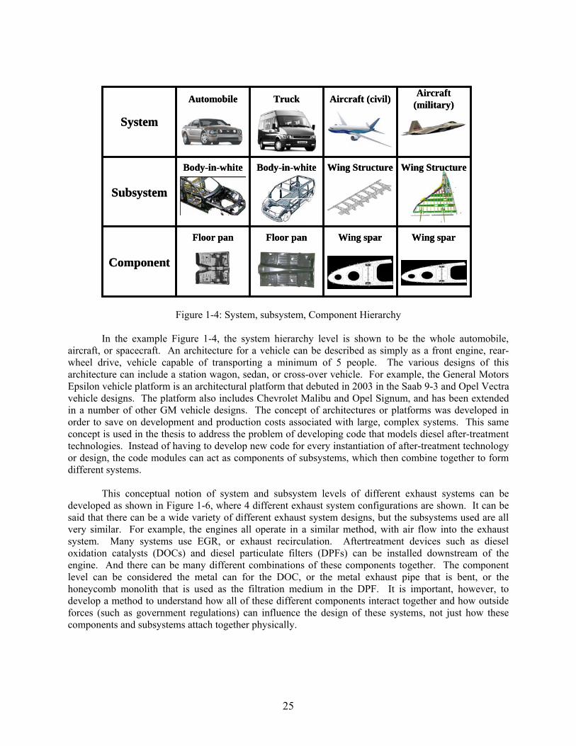
Figure 1-4: System, subsystem, Component Hierarchy
In the example Figure 1-4, the system hierarchy level is shown to be the whole automobile,
aircraft, or spacecraft. An architecture for a vehicle can be described as simply as a front engine, rear-wheel drive, vehicle capable of transporting a minimum of 5 people. The various designs of this architecture can include a station wagon, sedan, or cross-over vehicle. For example, the General Motors Epsilon vehicle platform is an architectural platform that debuted in 2003 in the Saab 9-3 and Opel Vectra vehicle designs. The platform also includes Chevrolet Malibu and Opel Signum, and has been extended in a number of other GM vehicle designs. The concept of architectures or platforms was developed in order to save on development and production costs associated with large, complex systems. This same concept is used in the thesis to address the problem of developing code that models diesel after-treatment technologies. Instead of having to develop new code for every instantiation of after-treatment technology or design, the code modules can act as components of subsystems, which then combine together to form different systems.
This conceptual notion of system and subsystem levels of different exhaust systems can be
developed as shown in Figure 1-6, where 4 different exhaust system configurations are shown. It can be said that there can be a wide variety of different exhaust system designs, but the subsystems used are all very similar. For example, the engines all operate in a similar method, with air flow into the exhaust system. Many systems use EGR, or exhaust recirculation. Aftertreatment devices such as diesel oxidation catalysts (DOCs) and diesel particulate filters (DPFs) can be installed downstream of the engine. And there can be many different combinations of these components together. The component level can be considered the metal can for the DOC, or the metal exhaust pipe that is bent, or the honeycomb monolith that is used as the filtration medium in the DPF. It is important, however, to develop a method to understand how all of these different components interact together and how outside forces (such as government regulations) can influence the design of these systems, not just how these components and subsystems attach together physically.
25

Engine
Engine
Engine
Engine DOC
DPFDOC
EGREGR
EGREGR
Exhaust After-treatment Systems With Different Architectures
Open Tailpipe:
EGR Only:
DOC Only:
EGR, DOC, DPF:
Figure 1-5: Conceptual Exhaust System Architectures
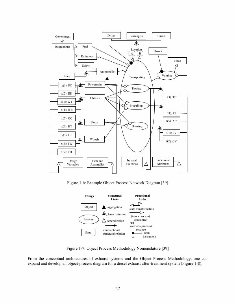
Expanding on the notion of a description for system architecture, it is important to think about
system (or product) architecture in terms of both form and function, and the connections between them. Object Process Methodology [11, 29, 45] has emerged as a formal graphical language for visualizing product architectures in terms of form (objects) and function (processes). Figure 1-7 in an example Object-Process Network of an automobile, at a very high level, where the object is decomposed into assemblies (modules), operands (driver, passenger, etc), internal functions (towing, driving), and its main value delivering function (transportation). A description of the nomenclature used in object process networks can be seen in Figure 1-7 .
It is important to understand that the main relationship between the component parts (objects)
and the functions (processes) can be mapped into the design variables of the product, x, and its functional attributes, f, which are associated with its internal functions. The same can be done at a smaller system level, such as the exhaust system. Once this is done, one can conceptually relate different physical conceptual architectures that most design engineers understand (Figure 1-5) to the objects and processes involved in the system, as shown in Figure 1-8 for the exhaust system example.
26
Driver
Figure 1-6: Example Object Process Network Diagram [39]
Figure 1-7: Object Process Methodology Nomenclature [39]
From the conceptual architectures of exhaust systems and the Object Process Methodology, one can expand and develop an object-process diagram for a diesel exhaust after-treatment system (Figure 1-8).
Object
Process
State
Things Structural Links
aggregation
characterization
generalization
unidirectional structural relation
Procedural Links
state transformation
(into a process) consumee
(out of a process) resultee
agentinstrument
Passengers Cargo
Location
Transporting
Automobile
Powertrain
Body
Chassis
Wheels
Propelling
Housing
Towing x(1): FC
x(2): ED
x(3): WT
x(4): WB
x(5): GC
x(6): HT
x(7): LT
x(8): TW
x(9): TD
Design Variables
Parts and Assemblies
Fuel
Emissions
Government
Regulations
Safety
A B
f(2): CV
f(1): PV
Owner
Internal Functions
f(3): TC
Valuing
Value
f(4): FE
f(5): AC
Functional Attributes
Price
27
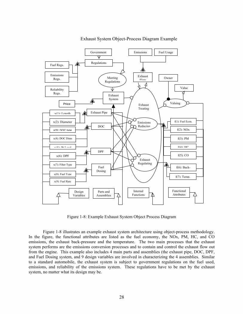
Exhaust System Object-Process Diagram Example
Figure 1-8: Example Exhaust System Object Process Diagram
Figure 1-8 illustrates an example exhaust system architecture using object-process methodology. In the figure, the functional attributes are listed as the fuel economy, the NOx, PM, HC, and CO emissions, the exhaust back-pressure and the temperature. The two main processes that the exhaust system performs are the emissions conversion processes and to contain and control the exhaust flow out from the engine. This example also includes 4 main parts and assemblies (the exhaust pipe, DOC, DPF, and Fuel Dosing system, and 9 design variables are involved in characterizing the 4 assemblies. Similar to a standard automobile, the exhaust system is subject to government regulations on the fuel used, emissions, and reliability of the emissions system. These regulations have to be met by the exhaust system, no matter what its design may be.
Fuel Usage Government Emissions
Exhaust Flow
Exhaust Treating
Exhaust System
Exhaust Pipe
DPF
DOC
Fuel Dosing
Emissions Reducing
Exhaust Regulating
x(1): Length
x(2): Diameter x(3): DOC type
x(4): DOC Dims
x(5): Pt Load
x(6): DPF
x(7): Filter Type
x(8): Fuel Type
x(9): Fuel Rate
Design Variables Parts and
Assemblies
Fuel Regs. Regulations
Emissions Regs.
Reliability Regs.
f(7): Temp. f(6): Back-
Internal Functions
Owner
Valuing
Value
f(4): HC
f(5): CO
Functional Attributes
Meeting Regulations
Price
f(3): PM f(2): NOx
f(1): Fuel Econ.
28

Figure 1-8 also illustrates two important concepts, that of design variables and functional attributes. The modeling methodology and framework developed in Chapter 3 takes the sample exhaust system object process diagram and extends it to being able to come up with the modeling framework for the exhaust system components. The design variables are used to characterize the components in the subsystems. The subsystems are then combined together to form the entire exhaust system model. This model can then be used to resolve the functional attributes of the system, from which the value of the exhaust system can then be derived.
One additional motivation to use MSDO is that the use of mathematical tools and methodologies in this manner is essential to resolving the cost and performance effectiveness of the design. One of the goals of MSDO is to be able to increase design freedom and knowledge about the product design throughout the design process. Generally speaking, there is more design knowledge known about a particular product and less design freedom as the product development process moves along from conception to realization. However, much of the products costs and design performances are significantly controlled by design choices made early on in the conception stage of the design process [13, 36].
Figure 1-9: Life Cycle Cost Commitment Versus Incurred Cost by Life Cycle Phase [36]
The fundamental problem is that poor design decisions early in the development process can lead
to costly mistakes later in the design process. This is illustrated in Figure 1-9, where typical design decisions made in the concept development stage significantly affect the determined cost of the system versus a comparatively low realization of product knowledge. The MSDO methodology has the ability to increase design freedom and knowledge earlier in the design process, in order to act on more information during a stage that significantly affects the determined cost of the system, as shown in Figure 1-10 [36].
29
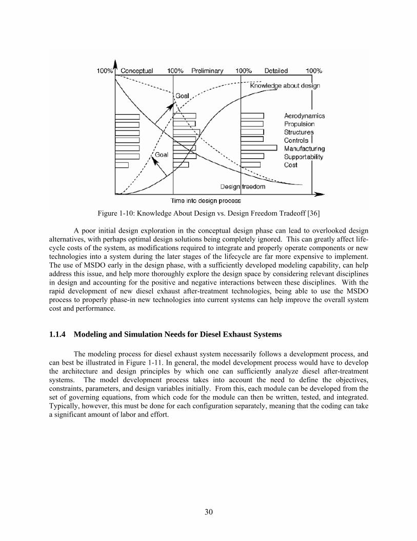
Figure 1-10: Knowledge About Design vs. Design Freedom Tradeoff [36]
A poor initial design exploration in the conceptual design phase can lead to overlooked design
alternatives, with perhaps optimal design solutions being completely ignored. This can greatly affect life-cycle costs of the system, as modifications required to integrate and properly operate components or new technologies into a system during the later stages of the lifecycle are far more expensive to implement. The use of MSDO early in the design phase, with a sufficiently developed modeling capability, can help address this issue, and help more thoroughly explore the design space by considering relevant disciplines in design and accounting for the positive and negative interactions between these disciplines. With the rapid development of new diesel exhaust after-treatment technologies, being able to use the MSDO process to properly phase-in new technologies into current systems can help improve the overall system cost and performance.
1.1.4 Modeling and Simulation Needs for Diesel Exhaust Systems
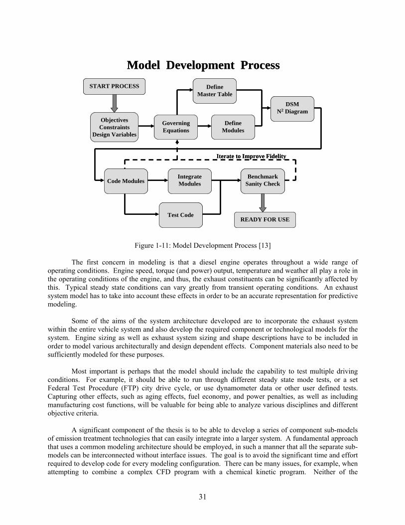
The modeling process for diesel exhaust system necessarily follows a development process, and can best be illustrated in Figure 1-11. In general, the model development process would have to develop the architecture and design principles by which one can sufficiently analyze diesel after-treatment systems. The model development process takes into account the need to define the objectives, constraints, parameters, and design variables initially. From this, each module can be developed from the set of governing equations, from which code for the module can then be written, tested, and integrated. Typically, however, this must be done for each configuration separately, meaning that the coding can take a significant amount of labor and effort.
30
Code Modules
Objectives Constraints
Design Variables
Governing Equations
Define Master Table
Define Modules
Integrate Modules
Test Code
Benchmark Sanity Check
READY FOR USE
DSM N2 Diagram
START PROCESS
Iterate to Improve Fidelity
Model Development Process
Code Modules
Objectives Constraints
Design Variables
Governing Equations
Define Master Table
Define Modules
Integrate Modules
Test Code
Benchmark Sanity Check
READY FOR USE
DSM N2 Diagram
START PROCESS
Iterate to Improve Fidelity
Model Development Process
Figure 1-11: Model Development Process [13]
The first concern in modeling is that a diesel engine operates throughout a wide range of
operating conditions. Engine speed, torque (and power) output, temperature and weather all play a role in the operating conditions of the engine, and thus, the exhaust constituents can be significantly affected by this. Typical steady state conditions can vary greatly from transient operating conditions. An exhaust system model has to take into account these effects in order to be an accurate representation for predictive modeling.
Some of the aims of the system architecture developed are to incorporate the exhaust system within the entire vehicle system and also develop the required component or technological models for the system. Engine sizing as well as exhaust system sizing and shape descriptions have to be included in order to model various architecturally and design dependent effects. Component materials also need to be sufficiently modeled for these purposes.
Most important is perhaps that the model should include the capability to test multiple driving conditions. For example, it should be able to run through different steady state mode tests, or a set Federal Test Procedure (FTP) city drive cycle, or use dynamometer data or other user defined tests. Capturing other effects, such as aging effects, fuel economy, and power penalties, as well as including manufacturing cost functions, will be valuable for being able to analyze various disciplines and different objective criteria.
A significant component of the thesis is to be able to develop a series of component sub-models of emission treatment technologies that can easily integrate into a larger system. A fundamental approach that uses a common modeling architecture should be employed, in such a manner that all the separate sub-models can be interconnected without interface issues. The goal is to avoid the significant time and effort required to develop code for every modeling configuration. There can be many issues, for example, when attempting to combine a complex CFD program with a chemical kinetic program. Neither of the
31
discipline’s detail is really required at the system level; instead a first order model is sufficient to capture the fluid and chemical kinetics. Once the major disciplines and governing equations are defined, the model should then be capable of using MDSO analysis to obtain the relative performance of various system designs, or even of different system architectures.
It is important to take into account a number of different aspects when building the models. First, a good baseline to start models is to base them on lumped parameter, first-order, control oriented models, using a basic ODE solver. These models work well for systems where flow quantities are passed from one component to another such as in fluids, power, and signal systems. Then from this model one can build more complex models with higher fidelity, as testing data becomes available and calibrations can be made to the original model. The models also need to capture the behavior of the component within the operating range of the system, and careful attention to simplifying assumptions and boundary conditions need to be made with each model. And while more fidelity and robustness can be introduced into the model development, care must be taken such that the computational effort required does not become overwhelming to the point where design optimization tasks become unwieldy.
1.2 Multidisciplinary Analysis and Design Optimization
1.2.1 MSDO and Optimization Methodology
The basic methodology of modeling and designing of complex engineering systems and subsystems is the integration of different modeling disciplines into a single model. This system model is a representation of a physical object that is composed of more than one element or component. These components combine together and exhibit behavior as a function of the interactions between them. Optimal design of complex engineering systems requires that the analysis accounts for interactions among the various components and a good understanding exists of the relations between the element components to be able to successfully model the various technologies in after-treatment systems.
The basic optimization methodology begins by first defining the design variables of such systems; that is a design vector x containing n variables that form the design space. The design space has to include any variables that a manufacturer or engineer has the ability to change, or that in one form or another, constitute a key design decision. During design space exploration or optimization we change the entries of x in some rational fashion to achieve the desired objectives. Within the optimization methodology, the objectives are defined as a vector J of z system responses or characteristics we are trying to maximize or minimize. Often the objective is a scalar function, but for real systems often we attempt multi-objective optimization to discover trade-offs, such as emission performance and cost objectives.
Finally, parameters, p, are defined as quantities that affect the objective J but are considered fixed, or otherwise unable to be changed at the engineer’s discretion. Sometimes parameters p can be turned into design variables xi to enlarge the design space, if this can be physically possible. Sometimes parameters p are former design variables that were fixed at some value because they were found not to affect any of the objectives Ji, or because their level was somehow determined a priori.
Constraints of the system act as boundaries of the design space x and typically occur due to finiteness of resources or technological limitations of some design variables. Often, but not always, optimal designs lie at the intersection of several active constraints. The source of constraints are often physical laws, such as considerations of mass, or man-made regulatory limits.
32
The Formal Notation of the optimization methodology is as follows [34]: minimize J(x,p) such that: g(x,p) ≤ 0 h(x,p) = 0 xi,LB ≤ xi ≤ xi,UB where: J = [J1(x) … Jz(x)]T x = [x1 … xi … xn]T
MSDO can mathematically trace paths in the design space from some initial design x0 towards improved designs (with respect to the objective J). It does this by being able to operate on a large number of variables and functions simultaneously, using the models developed for the system. This path instead of being invisible inside a “black box” becomes more visible by various MDO techniques such as sensitivity analysis and visualization. Optimization helps conduct trade studies in order to expand on the designer’s understanding of the system, and hopefully be able to allow designers to explore new directions of design or architecture.
There are three distinct components of the MSDO process: the model, simulation, and
optimization. The optimization algorithm decides how to move through the design space, but the simulation evaluates designs chosen by the optimizer, as shown in Figure 1-12. The model is the underlying static framework.
MSDO Framework
Discipline A
Discipline C
Discipline B
Out
put
Inpu
t
x1 x2
xn
…
J1 J2
Jn
…Design Vector Objective Vector
MultiobjectiveOptimization
Numerical Techniques
(Direct and Penalty Methods)
Heuristic Techniques
(SA, GA, etc)CouplingTradespace
Explortation(DOE)
Coupling
Optimization AlgorithmsApproximation
Methods
Sensitivity Analysis
Isoperformance
Special Techniques
MSDO Framework
Discipline A
Discipline C
Discipline B
Out
put
Inpu
t Discipline A
Discipline C
Discipline B
Out
put
Inpu
t
x1 x2
xn
…
x1 x2
xn
…
J1 J2
Jn
…J1 J2
Jn
…Design Vector Objective Vector
MultiobjectiveOptimization
Numerical Techniques
(Direct and Penalty Methods)
Heuristic Techniques
(SA, GA, etc)CouplingTradespace
Explortation(DOE)
Coupling
Optimization AlgorithmsApproximation
Methods
Sensitivity Analysis
Isoperformance
Special Techniques
Figure 1-12: MSDO Framework [13]
33
The challenges of MDO are that there is a tradeoff between the fidelity and computational expense of the disciplinary models that needs to be addressed. This extent of complexity can cause the analysis and optimization to be too slow to perform in a timely fashion to be able to give engineers the design space exploration required. Also, there are significant communication and user and software interface problems that each implementation of MSDO should address. Finally, the MSDO process should remain flexible throughout its evolution in order to allow for changes in the future.
1.2.2 Thesis Objectives and Goals
The thesis objective is to first develop a modeling and simulation methodology that employs systems thinking and MSDO to be able to sufficiently model diesel after-treatment technologies, with the end goal of comparative analysis between different architectures, designs, and applications of diesel exhaust systems. The hypothesis is that using this methodology, an engineer can accurately model and investigate different designs and be able to use optimization to refine designs in the early product development stage. The emphasis in this stage is on the relative comparison of architectures and designs, not on absolute forecasting, which can require different and more computational intensive analysis. This can, in turn, save on prototype and testing costs, while improving the performance in a wide variety of areas such as fuel economy and emissions performance.
Summarizing, the thesis is organized into four main parts: presenting the problem and
introduction, developing the modeling and analysis methodology, reviewing the results of the implementation, and the conclusion. A thesis map is shown in Figure 1-13 for a better illustration.
The first part, shown in Chapters 1 and 2, presents the problem and motivation, and presents the
engineering framework that can resolve the problem of advancing after-treatment technology for diesel engine vehicles. The engineering framework of systems analysis, system architecture, and multi-disciplinary system design and optimization (MSDO) were described in Chapter 1. The literature review highlights the prior approaches to diesel engine after-treatment technology modeling, and makes the point that there is very little prior work on combining the engineering framework of MSDO and systems thinking with diesel engine after-treatment systems.
From this overview, a flexible/modular design concept along with a state vector modeling
approach is used to develop the modeling framework. Once this framework is set-up, it is implemented in code (Chapters 3 and 4). Physical models and test data, along with prior research, is used to develop the model details and implemented in code. Chapter 3 also investigates the analysis techniques required for design optimization of after-treatment systems. A preliminary coarse optimization/exploration followed by an optimization refinement is presented.
Chapters 5 and 6 utilize the simulation code developed from the model details in two case studies.
First, Chapter 5 illustrates a single component model of an after-treatment system. Various designs are investigated, their trade-spaces analyzed, their performances calculated, and an optimization routine is run and the results presented. Chapter 6 includes a multi-component case study utilizing, and expands on Chapter 5’s implementation to investigate the interactions of a more complex system, that includes more inter-component interactions. Chapter 7 is a synthesis and summary of the conclusions the results gave for the thesis objectives.
34
Chapter 1: Overview & Motivation
Systems AnalysisMSDO
Systems ArchitectureSystems Analysis
MSDO
Systems Architecture
Diesel Engines
After-treatment Technology
Diesel Engines
After-treatment Technology
Reviewing Problem
Identifying Gap
Reviewing Problem
Identifying Gap
Chapter 3: Approach & Framework
Chapter 2: Literature
ReviewFlexible/Modular
Design
State Vector Modeling
Flexible/Modular Design
State Vector Modeling
Literature Review
Physical ModelsPhysical Models
Test DataTest Data
Implementing CodeAnalyzingImplementing
Framework Set-up
AnalyzingImplementing
Framework Set-up
Chapter 4: Model Details
Chapter 5: Single Component Case
Chapter 6: Multi-Component Case
Sim. CodeSim. CodeMulti-Component
ModelingMulti-Component
Modeling
Performance Objective Analysis
Developing Designs
Trade-space Analysis
Model Validation
Performance Objective Analysis
Developing Designs
Trade-space Analysis
Model Validation
Single Component Modeling
Single Component Modeling
Chapter 7: Synthesis and Conclusions
Generalizing
Synthesizing
Generalizing
Synthesizing
Figure 1-13: Thesis Map
Thesis Objectives:
• Develop a Modeling and Analysis Framework Based on a State Vector Approach. • Develop the Models of the Components and the Analysis Tools. • Integrate and Analyze the Problem using MSDO Methodology.
Thesis Hypotheses:
• System Analysis methodology can accurately model diesel exhaust system after-treatment technologies.
• MSDO Methodology can be used to compare and investigate exhaust system architectures • Design Optimization can be used to refine designs and link performance objectives to design
choices, and can uncover beneficial or harmful component interactions.
35
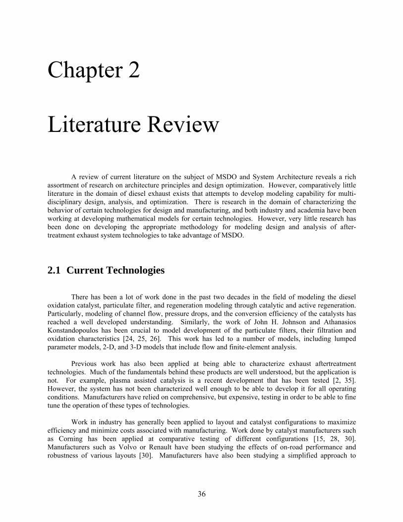
Chapter 2 . Literature Review
A review of current literature on the subject of MSDO and System Architecture reveals a rich
assortment of research on architecture principles and design optimization. However, comparatively little literature in the domain of diesel exhaust exists that attempts to develop modeling capability for multi-disciplinary design, analysis, and optimization. There is research in the domain of characterizing the behavior of certain technologies for design and manufacturing, and both industry and academia have been working at developing mathematical models for certain technologies. However, very little research has been done on developing the appropriate methodology for modeling design and analysis of after-treatment exhaust system technologies to take advantage of MSDO.
2.1 Current Technologies There has been a lot of work done in the past two decades in the field of modeling the diesel
oxidation catalyst, particulate filter, and regeneration modeling through catalytic and active regeneration. Particularly, modeling of channel flow, pressure drops, and the conversion efficiency of the catalysts has reached a well developed understanding. Similarly, the work of John H. Johnson and Athanasios Konstandopoulos has been crucial to model development of the particulate filters, their filtration and oxidation characteristics [24, 25, 26]. This work has led to a number of models, including lumped parameter models, 2-D, and 3-D models that include flow and finite-element analysis.
Previous work has also been applied at being able to characterize exhaust aftertreatment
technologies. Much of the fundamentals behind these products are well understood, but the application is not. For example, plasma assisted catalysis is a recent development that has been tested [2, 35]. However, the system has not been characterized well enough to be able to develop it for all operating conditions. Manufacturers have relied on comprehensive, but expensive, testing in order to be able to fine tune the operation of these types of technologies.
Work in industry has generally been applied to layout and catalyst configurations to maximize efficiency and minimize costs associated with manufacturing. Work done by catalyst manufacturers such as Corning has been applied at comparative testing of different configurations [15, 28, 30]. Manufacturers such as Volvo or Renault have been studying the effects of on-road performance and robustness of various layouts [30]. Manufacturers have also been studying a simplified approach to
36

modeling exhaust emission systems in the hopes of being able to achieve design optimization in terms of performance, cost, packaging, and control strategy [27, 31].
2.2 Future Technologies
There has been a lot of experimental work in continuous regenerating filter traps, selective catalyst reduction filters, and NOx traps. Although no one organization or academic institution has been spearheading significant innovation, much has been accomplished in testing and manufacturing. SCR has been introduced in concepts and is being currently tested in on-road applications by such companies as Corning, Engelhard, Johnson-Matthey, Dow Chemical, and others [32]. Many manufacturers are attempting to go into NOx Traps and Lean-NOx traps, as well as plasma technologies [2, 38]. Modeling and control studies of NOx trap catalysts have been done by manufacturers such as Ford and Renault [18, 22, 35]. Currently, there exists a large amount of literature and studies from which sub-model development for future technologies can be developed. But many manufacturers rely on empirical test data and a trial-and-error methodology at developing new technologies.
2.3 Modeling Research
Design and development of complex, interconnected systems can be difficult. Also, it is important to differentiate between the different types of models. Analysis models are important in that they describe the behavior of the system. Design and decision models are used to describe the design of a physical system and to give a measure of goodness of said design. Combining design, analysis, and decision (or optimization) models together can offer engineers a complete analysis and evaluation tool that can relate directly to design development [13, 29, 45].
The problem with modeling, however, is that in some cases a large degree of flexibility is required. Many discipline oriented analysis models do not allow for great flexibility for investigating design issues that deal with other disciplines. For example, a CFD model of exhaust gas flow is not useful when attempting to analysis the effects of muffler design on cost. A critical interface between the cost and flow modeling is required when combining these two detailed but discipline oriented models. Although product design flexibility has been rigorously studied, implementing flexibility in the modeling of products has not. Numerous authors have investigated module-based (configurable) product families [39].
By applying the methodologies previously described in Chapter 1 (MDO and Systems
Architecture), one can develop the framework for modeling exhaust aftertreatment technologies [11, 13, 29, 39, 45]. This framework can lead to better designs by combining the functional elements, mapping them to the physical components, specifying interfaces, and evaluating the interactions between the components. It allows for a more comprehensive, yet flexible, modeling approach where one can see the similarities between product development using platforming strategies, and the abstraction involved in modeling. By using a modular platform architecture in the modeling abstraction one can improve the flexibility and capability of the model to better simulate complex system models.
37

Chapter 3 . Approach and Framework
Part of the thesis objective and goals was to develop a series of sub-models for a set of emissions treatment technologies available and presently in-development. Then use these sub-models in a larger, system model of the entire emissions treatment system. A series of complete diesel emissions treatment system architectures can be constructed and analyzed, utilizing a multi-disciplinary, multi-objective system analysis methodology.
For system-wide, multi-disciplinary analysis there needs to be consideration given to the entire
vehicle system and its interaction with the environment and operating range and conditions. However, to simplify the system modeling, only the drivetrain, fuel injection system, and engine management system are considered to be the main factors in determining engine-out emissions to the exhaust system (given a certain vehicle/engine/drivetrain combination and drive cycle). To model the effects of the operation of the vehicle, simulations of standard drive cycles or actual engine dynamometer data can be used. Example engine-out emissions data from ADVISOR [1], a vehicle simulation program, can be used as inputs to the complete exhaust system models.
It is notable that a large number of exhaust system components can be sufficiently modeled parametrically, or within a 1-dimensional geometric description [40]. The majority of critical interactions can be reduced to the chemical conversion process of the exhaust gas species, the thermodynamics of reactions, and the heat and mass transfer. The filtration and trap models can be described using simple porous wall, layered filtration models, and in some cases even incorporating 1-dimensional length geometry in the flow-wise direction.
Fundamentally, these technological components can be described and modeled in an arrangement
of differential equations, with simple geometric variables and other parameters. Given the system-wide analysis viewpoint, there is no need for in-depth finite element modeling when these simpler models can be used to assemble together the entire system and give reasonable results for emissions and performance. Once architectures have been selected they can be modeled in greater detail. Although certain specific, local phenomena might be missed by the parametric modeling approach, at the high level it is not as important as gaining knowledge of the overall system behavior. For example, resolving the local flow and temperature distribution through all the channels in a catalyst may be important for verifying it does not overheat and maximizes longevity, it is not relevant when the system goal is to resolve the overall sizing and placement of the catalyst along the exhaust stream. Additionally, there is the need for the models to reflect varying environmental and operating conditions, and allow for fast computation in order to add-in optimization to the analysis methodology. A complete finite element model would be too complex and detailed for use in these instances, and the computational needs of the optimization requires focus on simple system modeling techniques.
38
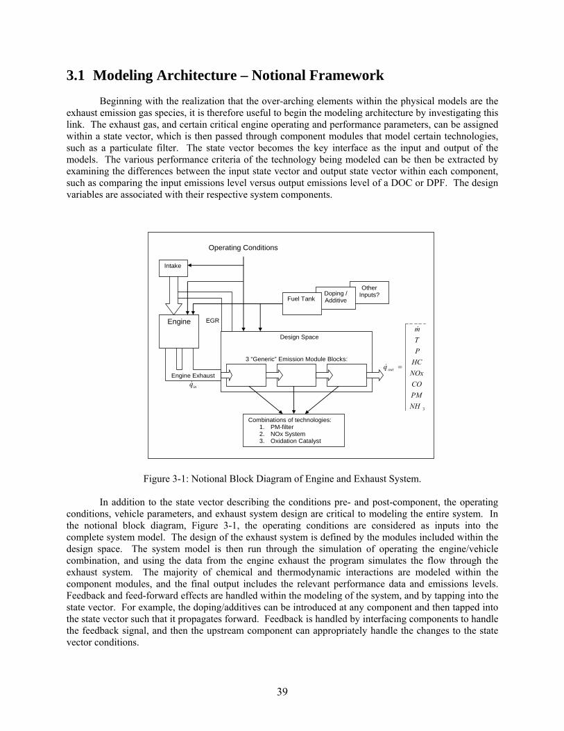
3.1 Modeling Architecture – Notional Framework
Beginning with the realization that the over-arching elements within the physical models are the exhaust emission gas species, it is therefore useful to begin the modeling architecture by investigating this link. The exhaust gas, and certain critical engine operating and performance parameters, can be assigned within a state vector, which is then passed through component modules that model certain technologies, such as a particulate filter. The state vector becomes the key interface as the input and output of the models. The various performance criteria of the technology being modeled can be then be extracted by examining the differences between the input state vector and output state vector within each component, such as comparing the input emissions level versus output emissions level of a DOC or DPF. The design variables are associated with their respective system components.
Other Inputs?
Design Space
3NHPMCONOxHCPTm
q out
&
& =
Doping / Additive
Engine
Intake
Engine Exhaust
inq&
EGR
Combinations of technologies: 1. PM-filter 2. NOx System 3. Oxidation Catalyst
3 “Generic” Emission Module Blocks:
Fuel Tank
Operating Conditions (T,P,ρ,AF,…)Operating Conditions
Figure 3-1: Notional Block Diagram of Engine and Exhaust System.
In addition to the state vector describing the conditions pre- and post-component, the operating conditions, vehicle parameters, and exhaust system design are critical to modeling the entire system. In the notional block diagram, Figure 3-1, the operating conditions are considered as inputs into the complete system model. The design of the exhaust system is defined by the modules included within the design space. The system model is then run through the simulation of operating the engine/vehicle combination, and using the data from the engine exhaust the program simulates the flow through the exhaust system. The majority of chemical and thermodynamic interactions are modeled within the component modules, and the final output includes the relevant performance data and emissions levels. Feedback and feed-forward effects are handled within the modeling of the system, and by tapping into the state vector. For example, the doping/additives can be introduced at any component and then tapped into the state vector such that it propagates forward. Feedback is handled by interfacing components to handle the feedback signal, and then the upstream component can appropriately handle the changes to the state vector conditions.
39

3.2 State Vector Platform Concept – State Vector as Interface
Within the exhaust system design space there are clear divisions (or modules) to be used for sub-model design. This “brick” division allows us to slice the design of the entire exhaust system into smaller parts, and modularly recombine the different components together to form different system architectures. For the purposes of the modeling, architecture is defined as the type and order of technological components within the exhaust system, whereas design of a system is defined as the description of the design variables for the components that make up said system. For example, one can have a diesel oxidation catalyst (DOC) model followed by a particulate filter (DPF), or swap the components for a different architecture. This allows us to treat the exhaust system as a linear combination of elements, with the state vector passing through each component. The state vector is not only used to transfer information to and from component, but is used as the platform from which all the different physical models are built. So the state vector is always had for a component’s constitutive model, even if a component does not act upon (is inert) some of the state vector’s components. The state vector defines the key interfaces of data from which all the component models can then perform the appropriate computations. Figure 3-2 shows a 2-module system, with an input data file, two in-line DOC (diesel oxidation catalyst) modules, and a “tailpipe out” emissions output data file.
Chemical Reactions
Thermo Reactions
Module (DOC)
Chemical Reactions
Thermo Reactions
Module (DOC)
Advisor EO Emissions Data File
ADVISOR Drive Cycle Simulation Data
Exhaust Emissions Data File
2-Module Exhaust Systems I/O Process
Feedback
Figure 3-2: “Module” Architecture of Exhaust System Components. Example 2-Module Exhaust System with inputs and outputs modeled.
There is consideration for global feedback, specifically engine operation control from exhaust
component feedback. In this case, since the engine emission file is set, the effect of the feedback on the exhaust gas flow has to be characterized, and those effects are implemented as changes to the state vector within the exhaust system model. In a broader implementation, the engine model can be included directly, and thus account for the global feedback directly.
The state vector has included two main set of components that are required, at the present time to sufficiently describe the exhaust gas flow in physical terms, that of the chemical species and the thermodynamic parameters. Table 3-1 lists the data included in the current state vector formulation.
40
Table 3-1: State Vector Components State Vector Component Unit Description and Notes
Time Stamp sec Simulation time (in seconds), required for time-based modeling Engine on signal 1,0 Describes in binary format if engine is on or off. Intended use is as a
signal, more normally used in case of hybrid engine configurations. HC – hydrocarbons g/s Hydrocarbon gas mass flow; chief pollutant CO – carbon monoxide g/s Carbon monoxide gas mass flow; chief pollutant NOx – oxides of nitrogen g/s Oxides of nitrogen; chief pollutant; Generally sum of NO and NO2PM – particulate matter g/s Particulate matter; chief pollutant Exhaust gas mass flow g/s Aggregate mass flow Exhaust gas temperature deg C Lumped exhaust gas temperature Oxygen mass flow g/s Oxygen concentration (in mass flow terms) in exhaust gas Vehicle speed m/s Used to track vehicle from drive cycle operation; also used for heat
transfer from exhaust system to airflow Temperature – previous component
deg C Used to track component to component temperatures (averaged value) at the interfaces between components
Diesel fuel (liquid) g/s Tracks any liquid diesel fuel injected or otherwise part of exhaust gas flow
CO2 g/s Component of rack emission measurements, Carbon dioxide H2O g/s Component of rack emission measurements, water N2 g/s Component of rack emission measurements, nitrogen NO g/s Component of NOx emissions. NO2 g/s Component of NOx emissions. SO2 g/s Sulfur dioxide is used for emission tracking and adverse to the life of
catalysts and filters NH3 g/s Ammonia gas is used in combination with Urea in SCR-DPF systems. Urea g/s Urea is a chemical used in SCR DPF systems for regeneration H2 g/s Component of rack emission measurements H2S g/s Hydrogen sulfide is used for other emissions and adverse to catalyst
life. SMD M Sauter mean diameter – used for tracking fuel spray and other
combustion processes in exhaust system Exhaust Gas Pressure Pa Exhaust gas state parameter Mass flow diesel fuel g/s Tracks diesel fuel flow rate into engine Engine Speed RPM Tracks engine speed in revolutions per minute Engine Torque Output Nm Tracks engine torque output.
41

3.2.1 Operating State Vector Model
System Design Space
Modules consisting of exhaust components from libraries
ReportsReports
State Vector
Out Data
State Vector
Out Data
State Vector In Data
State Vector In Data
Model LibraryController LibraryOther Inputs
Model LibraryController LibraryOther Inputs
Engine LibraryDrive-cycle LibraryOperating Conditions
Engine LibraryDrive-cycle LibraryOperating Conditions
EO Data File (xls)EO Data File (xls)
Feedback Considerations
Figure 3-3: Complete System Model Flow Diagram
The exhaust system model will function by using an input file describing the engine exhaust conditions over time. This input file contains all the required information about the exhaust gas flow, given a certain engine/vehicle combination, and its performance over time in a given operating regime – it contains the state vector parameters at the engine output. The operating regime, or drive cycle, used for the engine simulation can be steady state conditions or transient, as the input file is a time-based discretization of the state of the exhaust gas flow. The input file data can be based from actual test data or simulation. Particularly effective at modeling the engine parameters is a simulation software package called ADVISOR that can be used to model different engine/vehicle combinations under different operating regimes or drive cycles. The vehicle models used in ADVISOR include all of the relevant engine-out emissions data per time-increment of a specific drive cycle. The input file (shown as the “EO Data File” in Figure 3-3) is constructed from a library of engine and drive-cycle files, as required by the user, and typically has a time step of one second in order to account for transient behaviors of drive cycles.
The system program then converts the information from the input data file into the state vector,
which is operated on sequentially through the complete exhaust system model. The system model (shown as the System Design Space in Figure 3-3), is built from the “model and controller library.” Different technologies are modeled, along with the requisite active controllers, and this library is sourced to build the exhaust system model. The system models use ODE solvers included in Matlab/Simulink (such as a simple discrete solver, Euler, or Heun solver) to execute the simulation on a fixed time step basis.
After the simulation ends, the program will make an output file, from which reports of
performance data can be extracted. The output data, along with data from within the model, can be used to validate and tune the model to the actual components in production or under development.
42
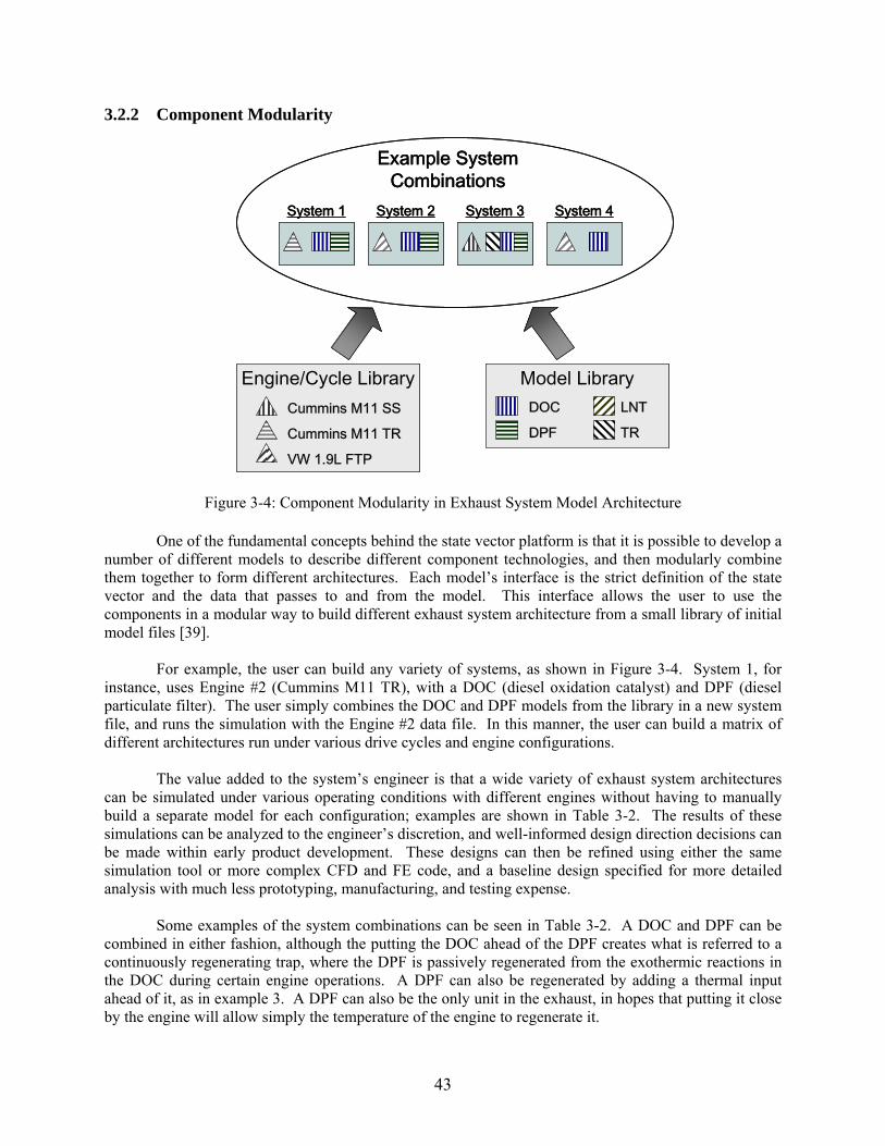
3.2.2 Component Modularity
Model LibraryDOC LNT
DPF TRCummins M11 SS
Cummins M11 TR
VW 1.9L FTP
Engine/Cycle Library
System 2 System 3 System 1
Example System Combinations
System 4
Model LibraryDOC LNT
DPF TRCummins M11 SS
Cummins M11 TR
VW 1.9L FTP
Engine/Cycle Library
System 2 System 3 System 1
Example System Combinations
System 4
Figure 3-4: Component Modularity in Exhaust System Model Architecture
One of the fundamental concepts behind the state vector platform is that it is possible to develop a number of different models to describe different component technologies, and then modularly combine them together to form different architectures. Each model’s interface is the strict definition of the state vector and the data that passes to and from the model. This interface allows the user to use the components in a modular way to build different exhaust system architecture from a small library of initial model files [39].
For example, the user can build any variety of systems, as shown in Figure 3-4. System 1, for
instance, uses Engine #2 (Cummins M11 TR), with a DOC (diesel oxidation catalyst) and DPF (diesel particulate filter). The user simply combines the DOC and DPF models from the library in a new system file, and runs the simulation with the Engine #2 data file. In this manner, the user can build a matrix of different architectures run under various drive cycles and engine configurations.
The value added to the system’s engineer is that a wide variety of exhaust system architectures
can be simulated under various operating conditions with different engines without having to manually build a separate model for each configuration; examples are shown in Table 3-2. The results of these simulations can be analyzed to the engineer’s discretion, and well-informed design direction decisions can be made within early product development. These designs can then be refined using either the same simulation tool or more complex CFD and FE code, and a baseline design specified for more detailed analysis with much less prototyping, manufacturing, and testing expense.
Some examples of the system combinations can be seen in Table 3-2. A DOC and DPF can be
combined in either fashion, although the putting the DOC ahead of the DPF creates what is referred to a continuously regenerating trap, where the DPF is passively regenerated from the exothermic reactions in the DOC during certain engine operations. A DPF can also be regenerated by adding a thermal input ahead of it, as in example 3. A DPF can also be the only unit in the exhaust, in hopes that putting it close by the engine will allow simply the temperature of the engine to regenerate it.
43
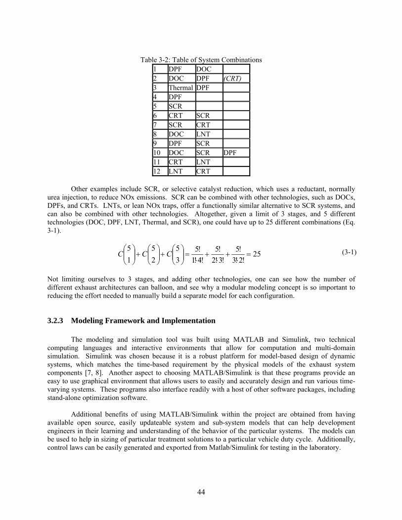
Table 3-2: Table of System Combinations
1 DPF DOC 2 DOC DPF (CRT) 3 Thermal DPF 4 DPF 5 SCR 6 CRT SCR 7 SCR CRT 8 DOC LNT 9 DPF SCR 10 DOC SCR DPF 11 CRT LNT 12 LNT CRT
Other examples include SCR, or selective catalyst reduction, which uses a reductant, normally
urea injection, to reduce NOx emissions. SCR can be combined with other technologies, such as DOCs, DPFs, and CRTs. LNTs, or lean NOx traps, offer a functionally similar alternative to SCR systems, and can also be combined with other technologies. Altogether, given a limit of 3 stages, and 5 different technologies (DOC, DPF, LNT, Thermal, and SCR), one could have up to 25 different combinations (Eq. 3-1).
25!2!3
!5!3!2
!5!4!1
!535
25
15
=⋅
+⋅
+⋅
=⎟⎟⎠
⎞⎜⎜⎝
⎛+⎟⎟
⎠
⎞⎜⎜⎝
⎛+⎟⎟
⎠
⎞CC⎜⎜
⎝
⎛C
Not limiting ourselves to 3 stages, and adding other technologies, one can see how the numbdifferent exhaust architectures can balloon, and see why a modular modeling concept is so importreducing the effort needed to manually build a separate model for each configuration.
3.2.3 Modeling Framework and Implementation
The modeling and simulation tool was built using MATLAB and Simulink, two techcomputing languages and interactive environments that allow for computation and multi-dosimulation. Simulink was chosen because it is a robust platform for model-based design of dynsystems, which matches the time-based requirement by the physical models of the exhaust sycomponents [7, 8]. Another aspect to choosing MATLAB/Simulink is that these programs provieasy to use graphical environment that allows users to easily and accurately design and run various varying systems. These programs also interface readily with a host of other software packages, inclstand-alone optimization software.
Additional benefits of using MATLAB/Simulink within the project are obtained from h
available open source, easily updateable system and sub-system models that can help developengineers in their learning and understanding of the behavior of the particular systems. The modelbe used to help in sizing of particular treatment solutions to a particular vehicle duty cycle. Additiocontrol laws can be easily generated and exported from Matlab/Simulink for testing in the laboratory
44
(3-1)
er of ant to
nical main amic stem
de an time-uding
aving ment s can nally, .
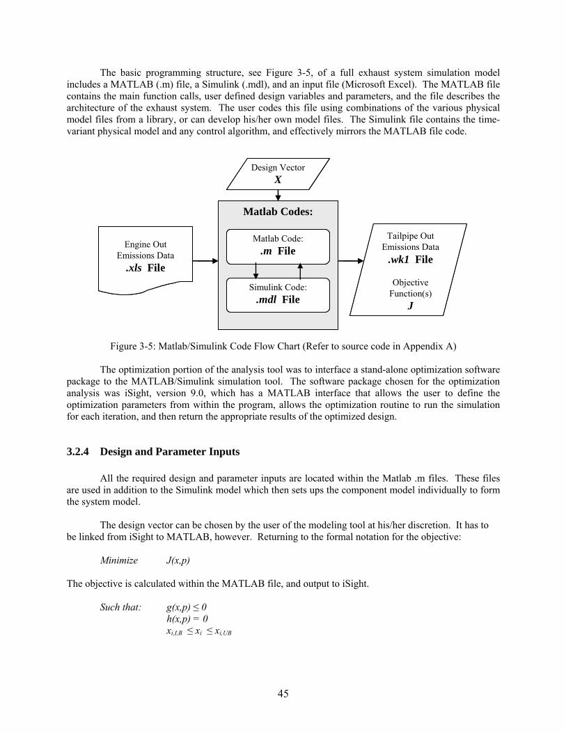
The basic programming structure, see Figure 3-5, of a full exhaust system simulation model includes a MATLAB (.m) file, a Simulink (.mdl), and an input file (Microsoft Excel). The MATLAB file contains the main function calls, user defined design variables and parameters, and the file describes the architecture of the exhaust system. The user codes this file using combinations of the various physical model files from a library, or can develop his/her own model files. The Simulink file contains the time-variant physical model and any control algorithm, and effectively mirrors the MATLAB file code.
Matlab Codes:
Simulink Code:.mdl File
Tailpipe Out Emissions Data
.wk1 File
Objective Function(s)
J
Engine Out Emissions Data
.xls File
Design Vector X
Matlab Code:.m File
Matlab Codes:
Simulink Code:.mdl File
Simulink Code:.mdl File
Tailpipe Out Emissions Data
.wk1 File
Objective Function(s)
J
Engine Out Emissions Data
.xls File
Engine Out Emissions Data
.xls File
Design Vector X
Design Vector X
Matlab Code:.m File
Matlab Code:.m File
Figure 3-5: Matlab/Simulink Code Flow Chart (Refer to source code in Appendix A)
The optimization portion of the analysis tool was to interface a stand-alone optimization software
package to the MATLAB/Simulink simulation tool. The software package chosen for the optimization analysis was iSight, version 9.0, which has a MATLAB interface that allows the user to define the optimization parameters from within the program, allows the optimization routine to run the simulation for each iteration, and then return the appropriate results of the optimized design.
3.2.4 Design and Parameter Inputs
All the required design and parameter inputs are located within the Matlab .m files. These files are used in addition to the Simulink model which then sets ups the component model individually to form the system model.
The design vector can be chosen by the user of the modeling tool at his/her discretion. It has to be linked from iSight to MATLAB, however. Returning to the formal notation for the objective: Minimize J(x,p) The objective is calculated within the MATLAB file, and output to iSight. Such that: g(x,p) ≤ 0 h(x,p) = 0 xi,LB ≤ xi ≤ xi,UB
45

The g(x,p), and h(x,p), constraints are identified and calculated within MATLAB. Although the optimizer may or may not take these into account, depending on the physical applicability of the model. The bounds are identified within iSight. Where: J = [J1(x) … Jz(x)]T x = [x1 … xi … xn]T
Again, both the Objective Matrix and Design Vector are identified in MATLAB, and used by iSight. MATLAB acts an interface between the iSight optimizer and the Simulink system model. The following graphic shows the domains of the programs, using the MSDO framework diagram. Figure 3-6 illustrates the domain of MATLAB, Simulink, and iSight, with respect to each other, and what program controls what aspect of the MSDO methodology. The major interface between MATLAB and iSight remains the design and objective vectors, whereas MATLAB and Simulink remain part of a highly interfaced simulation model.
MSDO Framework and Software Domain
Discipline A
Discipline C
Discipline B
Out
put
Inpu
t Discipline A
Discipline C
Discipline B
Out
put
Inpu
t
x1 x2
xn
…
x1 x2
xn
…
J1 J2
Jn
…
J1 J2
Jn
…
Design Vector Objective Vector
MultiobjectiveOptimization
Numerical Techniques
(Direct and Penalty Methods)
Heuristic Techniques
(SA, GA, etc)CouplingTradespace
Explortation(DOE)
Coupling
Optimization Algorithms
Matlab and SimulinkMatlab and iSight
iSight
Matlab and iSight
Figure 3-6: MSDO Mapping to Software Code
46

The design space exploration, optimization algorithms, multi-objective optimization and other special techniques remain within the domain of specialty software. The benefit of this is that the specialty software can remain a dedicated optimizer, whereas MATLAB/Simulink remains the simulation engine. In fact, iSight can be replaced at later dates by other specialty, stand-alone, optimization software, and perhaps other users may use MATLAB’s own optimization toolbox and utilities. Using MATLAB as the simulation model software allows for a wide degree of flexibility in software usage in the future.
3.3 Optimization Approach
3.3.1 Framework Flow Chart and Optimization Implementation
By extending the differentiating domain concept from Figure 3-5, the optimization implementation can be summarized in the Figure 3-7 flow chart.
Matlab Codes:
Simulink Code:.mdl File
Tailpipe Out Emissions Data
.wk1 File
Objective Function(s)
J
Engine Out Emissions Data
.xls File
Design Vector X
Matlab Code:.m File
User:Defines Initial Design and Begins
Optimization Routine
Optimization (iSight) Codes:
iSight Files
Algorithms and Convergence Criteria
.desc File
Design Vector
Parameters
X0
Converged?No
Yes
“Best” Design Vector XBest
“Best” Objective Function(s) JBest
Report Produced:Best Design, Performance Values, &
Objective Function Values
Matlab Codes:
Simulink Code:.mdl File
Simulink Code:.mdl File
Tailpipe Out Emissions Data
.wk1 File
Objective Function(s)
J
Engine Out Emissions Data
.xls File
Engine Out Emissions Data
.xls File
Design Vector X
Design Vector X
Matlab Code:.m File
Matlab Code:.m File
User:Defines Initial Design and Begins
Optimization Routine
Optimization (iSight) Codes:
iSight Files
Algorithms and Convergence Criteria
.desc File
Design Vector
Parameters
X0
Converged?No
Yes
“Best” Design Vector XBest
“Best” Objective Function(s) JBest
“Best” Design Vector XBest
“Best” Objective Function(s) JBest
Report Produced:Best Design, Performance Values, &
Objective Function Values
Figure 3-7: System Simulation Flow Diagram.
47
Typically, the user can define the starting design point, and begins the optimization routine. iSight will run the optimization routine, set-up the design vector and parameters, operate the optimization algorithm, output and run the design vector to MATLAB/Simulink, return the objective function then calculated back to the optimization algorithm code, and finally return the results when converged upon a solution (or the termination criteria reached).
3.3.2 Algorithm Choice
Choosing the appropriate optimization algorithm is critical in being able to do fulfill a satisfactory design space exploration and yield the appropriate and correct objective (local minimum or maximum). Generally, a heuristic algorithm is necessary in initial design space exploration and optimization because of the strength of this type of algorithm. Heuristic algorithms are typically used to solve complex (large, nonlinear, nonconvex) multivariate combinatorial optimization problems that are difficult to solve to optimality. They are good at dealing with local optima in that they avoid getting stuck in them while searching for the global optimum. However, there is no guarantee that the heuristic algorithm is going to find the true global optimal solution [13, 34]. Therefore, it is imperative that the results of the heuristic algorithm be analyzed for two aspects by the engineer before the decision on what to pursue for a non-linear programming optimization method is used [34].
The first part of the heuristic optimization is to search the tradespace in a coarse manner, in order to obtain a reasonable understanding of the tradeoffs between objectives and design variables, as shown in Step 1 of Figure 3-8. Given that this is a multi-objective problem, the objective space is searched for tradeoffs between competing objectives, as well as solving for the best compromise or optimality between objectives. Once the objective space results are analyzed the design space results are examined for correlations between competing performance objectives and, ideally, for resulting solutions of design families, as shown by Step 2 in Figure 3-8. It is important to understand how these optimal design families correspond to the performance objectives in order for engineers to better understand the interactions of the system as a whole.
48

Initial Design Exploration and Optimization Results
STEP 1: Heuristics Based
Optimization
STEP 2:
Design Family 1 Design Family 2 Design Family 3
STEP 3: Gradient Based
Optimization
Design Family Choices
Figure 3-8: Algorithm Steps
The search for design families is also critical in being able to then identify designs with potential for various applications, as well as the ability to be easily adapted later on in the life cycle. Design families are sought after in industry due to their cost effectiveness in manufacturing and ability to generate multiple products using very similar, if not the same, components. Generally, design families are designs with a set of similar design variables. This set of similar parameters or variables can be held constant in order to ease manufacturing and reduce costs, but allow other design variables to vary with specific applications. For example, if a certain DOC size is found to perform well in conjunction with a set of different DPFs, then different CRT products can be made by varying the DPF while keeping the DOC construction identical.
Once the second step of identifying and choosing design families is complete, along with the
appropriate performance objectives, then a local objective space optimization can be performed that will yield a finer analysis, with greater emphasis placed on finding that design’s local optimum, as shown in Step 3 of Figure 3-8. For this optimization analysis, a non-linear sequential quadratic programming optimization algorithm can be applied. The reason for using a gradient based optimization at this point is to guarantee that the local optimum is found for the particular design family. Additionally, performance objectives can be varied to suit a particular problem or design family solution set.
49

Chapter 4 . Model Components
The modeling details for the diesel exhaust technologies implemented in the modeling and
simulation program are summarized in this chapter. More detailed model information is available in Appendix A. Additionally, this chapter reviews a validation of two such models, a DOC and DPF, with simulation results, test data, and the manufacturer’s specifications. Other components are possible, but not modeled in detail in this chapter.
4.1 Diesel Oxidation Catalyst (DOC)
The diesel oxidation catalyst model is based on the chemical reactions of converting pollutant gaseous species (carbon monoxide (CO), hydrocarbons (HC), and oxides of nitrogen (NOx)) to nitrogen dioxide (NO2), carbon dioxide, and water [1, 15, 27, 30, 31, 37, 42, 44]. The basics chemical reactions are described as the following three equations. (Note that in this case, the hydrocarbons (HC) are described as C3H6.)
CO + ½ O2 CO2C3H6 + 9/2 O2 3 CO2 + 3 H2O
NO + ½ O2 NO2
In addition, the thermal behavior of the catalytic converter is modeled by the thermal behavior of the chemical reactions in addition to the heat loss through the catalyst (by way of conduction, convective, and radiative heat transfer). Combining these chemical kinetic and thermodynamic equations together within MATLAB/Simulink and iterating over time allows the model to be a computational simple and easy to use dynamic model. The basic assumptions of the model are as follows:
• Temperatures, concentrations, and spatial velocities are assumed to be the cross-sectional averaged quantities, effectively making this a 1-D, flow-through model.
• Radial and axial gradients are neglected. • Exhaust gas properties varies with temperature and mole fraction of species (effectively exhaust
gas species concentration). • Quasi-steady-state assumed. • The reactions are assumed to be second order (first order with respect to O2 mole fraction, and
first order with respect to the specific species mole fraction involved in the reaction). • Reaction rate constants and adsorption equilibrium constants follow the Arrhenius form.
50
• Oxidation of CO into CO2 is simplified (rate based Arrhenius form) • HC oxidation is also simplified, since typical HC diesel exhaust distributions range between C1
and C40, but are centered in the C9-C12 range. Since HC emissions are already low, quantifying HC emissions in C9-C12 range would be difficult to model, and therefore a lower molecular weight was selected. HC second order effects are assumed to be negligible.
• Sulfur, in form of sulfur dioxide was neglected. • Nitric oxide and NO2 are assumed as representative of all the nitrogen oxides (NOx).
The reaction rate constants are assumed to follow an Arrhenius form, as generally described
below:
RTE
Ri
Ri
eA−
=ik
Or
(4-1)
E is activation energy, R is the universal gas constant, and A is the pre-exponential factor. Given that A,R, and E are all constants, then the reactions are purely a function of temperatures and gas species concentrations, which allows for simplification of the model.
The oxygen (O2) consumption rate, an important parameter to track given the lean state of the exhaust gas and the availability of oxygen for reactions, is obtained by assuming stoichiometric reaction of the three main chemical conversion reactions, and is given by Eq. (4-2).
NOxHCCO rrr ⋅+⋅+⋅= 5.05.45.02
(4-3)).
(4-2)
Also, the assumption that the rate of transport of species from exhaust gases is equal to the rate of disappearance of species due to reaction on the monolith wall can be made, and therefore, the reaction rate can be finally expressed as the following (for each species, i), as a function of concentration and gas properties (Eq.
(4-3) iigisim rYYk
RTP
−=−⋅⋅⎟⎠⎞ )( ,,,⎜
⎝⎛
im&
This equation gives the reaction rate of the conversion of the exhaust gas species, and thus discrete integration of this equation over time steps within MATLAB/Simulink will give the conversion between incoming and exiting pollutant exhaust gas species concentrations.
The basic metric for resolving the conversion efficiency of the exhaust gas species is to compare the mass flows in versus out of the converter, as shown by Eq. (4-4):
(4-4) iniiout m __ )1( &η−=
The variable, i, identifies the four (4) main emission gas species (NOx, HC, CO, and PM), and where η is the conversion efficiency of the catalyst for that particular gas species. From the reaction rates described above, the conversion efficiency is fundamentally a function of temperature, catalyst formulation, and gas species concentration.
),,( λη catalystTempf= (4-5)
51
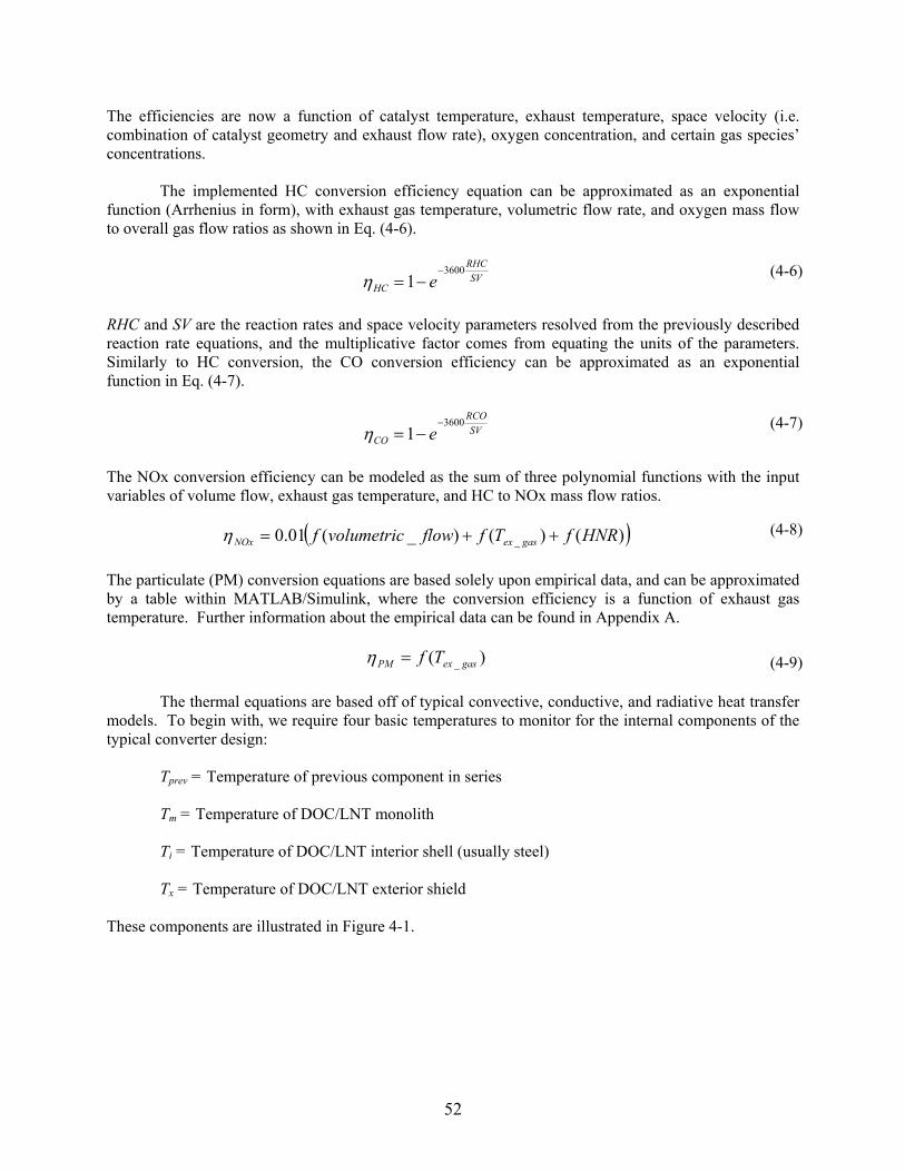
The efficiencies are now a function of catalyst temperature, exhaust temperature, space velocity (i.e. combination of catalyst geometry and exhaust flow rate), oxygen concentration, and certain gas species’ concentrations.
The implemented HC conversion efficiency equation can be approximated as an exponential function (Arrhenius in form), with exhaust gas temperature, volumetric flow rate, and oxygen mass flow to overall gas flow ratios as shown in Eq. (4-6).
SVRHC
e3600
1−
−=HCη (4-6)
RHC and SV are the reaction rates and space velocity parameters resolved from the previously described reaction rate equations, and the multiplicative factor comes from equating the units of the parameters. Similarly to HC conversion, the CO conversion efficiency can be approximated as an exponential function in Eq. (4-7).
SVRCO
e3600
1−
−=COη (4-7)
The NOx conversion efficiency can be modeled as the sum of three polynomial functions with the input variables of volume flow, exhaust gas temperature, and HC to NOx mass flow ratios.
( ))()()_(01.0 _ HNRfTfflowvolumetricf gasexNOx ++=η (4-8)
The particulate (PM) conversion equations are based solely upon empirical data, and can be approximated by a table within MATLAB/Simulink, where the conversion efficiency is a function of exhaust gas temperature. Further information about the empirical data can be found in Appendix A.
)( _ gasexTfPM =η (4-9)
The thermal equations are based off of typical convective, conductive, and radiative heat transfer models. To begin with, we require four basic temperatures to monitor for the internal components of the typical converter design:
Tprev = Temperature of previous component in series Tm = Temperature of DOC/LNT monolith Ti = Temperature of DOC/LNT interior shell (usually steel) Tx = Temperature of DOC/LNT exterior shield
These components are illustrated in Figure 4-1.
52

DOC Heat Shield
Figure 4-1: Diesel Oxidation Catalyst Component Diagram
Basic heat flow equations give the following differential equations:
( )
∫ ⋅
+−=
initT monmon
mongastomoncatmon dt
CpmQQQ
T_
__&&&
=mT
∫ ⋅=
initT
dtCpm
QT
_ intint
intint
&=iT
∫ ⋅=
initT extext
extext dt
CpmQ
T_
&=xT
Q =&
The heat flux equations are a function of constants, temperatures, and geometric variations:
),,,,( geometriesThekf ∆ The constants are k, thermal conductivity, e, emissivity, and h, convective coefficients, and can be approximated from texts or calibrated to match empirical data (refer to Appendix A for more information).
The pressure loss through the catalytic converter can be approximated by the typical automotive-monolith, channel flow theory. The pressure loss of assumed fully developed laminar channel flow is described by the Hagen-Poiseuille equation:
⎟⎟⎠
⎞⎜⎜⎝
⎛⋅
⋅⎟⎠⎞
⎜⎝⎛=
hdLPoV
Re4
21 2ρ∆P
Po is the Poiseuille number, L is the channel length, V is the exhaust gas velocity, ρ is the densityRe is the Reynolds number, and dh is the channel hydraulic diameter. To account for devboundary layers in the pressure loss relationship, an additional term is added, Kz, the Shah correlachannel to Eq. (4-14) (refer to Appendix A). The summation of all the channels in the monolith bthe pressure drop through the entire DOC monolith.
DOC Monolith DOC Shell
Previous component
flow
(4-10)
(4-11)
(4-12)
(4-13)
)
53
(4-14
of air, eloping tion per ecomes

4.2 Diesel Particulate Filter (DPF)
The model developed to describe the behavior a DPF during the loading and regeneration process is based on a 0-D, lumped parameter analysis that included a filtration model [9, 10, 16, 17, 20, 24, 25, 26, 31, 33, 42, 44]. The model assumes that the total volume of the filter is the control volume, and that the only spatial variance is the distribution of the particulate mass through the filter’s walls. The major assumptions are as follows:
• The filtration model used for calculating the filter collection efficiency treats the ceramic walls as a packed bed of uniform spherical collectors. Brownian diffusion and direct interception are assumed to be the two dominant collection mechanisms.
• The pressure drop through the filter is modeled using fluid dynamic flow through channels using the physical properties of the monolith, in addition to temperature and collected particulate mass effects.
• The particulate mass collected in the filter is distributed evenly radially and axially through the filter, and is only spatially described through the thickness of the wall.
• The temperature of the filter does not have a spatial variation, but it does vary between the major components of the filter (e.g. insulation, monolith, exterior shell, etc.)
4.2.1 Filtration Sub-Model The filtration model is divided into two regimes, the particulate that’s collected within the filter wall, and the particulate that collects on the surface of the filter wall. Within the wall, the model discretizes the filter wall along its thickness into slabs, as shown in Figure 4-2. And then within each slab, the microstructure of the model is based on a “unit collection” mechanism, with Brownian and direct interception models for the collection efficiency.
Figure 4-2: Layered wall structure
inm&
inmE &1
inmEm && )1( 12 −=
inm&
ii mE &
iiout mEm && )1( −=
x11
x2
2 x3
3 x4
4
xi i
xi+1
54
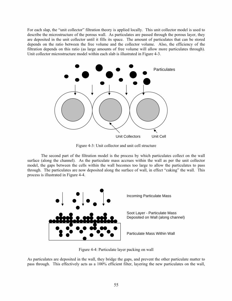
For each slap, the “unit collector” filtration theory is applied locally. This unit collector model is used to
The second part of the filtration model is the process by which particulates collect on the wall
urface
s particulates are deposited in the wall other particulate matter to
describe the microstructure of the porous wall. As particulates are passed through the porous layer, they are deposited in the unit collector until it fills its space. The amount of particulates that can be stored depends on the ratio between the free volume and the collector volume. Also, the efficiency of the filtration depends on this ratio (as large amounts of free volume will allow more particulates through). Unit collector microstructure model within each slab is illustrated in Figure 4-3.
Particulates
Figure 4-3: Unit collector and unit cell structure
s (along the channel). As the particulate mass accrues within the wall as per the unit collector model, the gaps between the cells within the wall becomes too large to allow the particulates to pass through. The particulates are now deposited along the surface of wall, in effect “caking” the wall. This process is illustrated in Figure 4-4.
Unit Cell Unit Collectors
Particulate Mass Within Wall
Incoming Particulate Mass
Soot Layer - Particulate Mass nel) Deposited on Wall (along chan
Figure 4-4: Particulate layer packing on wall
A , they bridge the gaps, and prevent the pass through. This effectively acts as a 100% efficient filter, layering the new particulates on the wall,
55

along the channel. This mechanism also increases pressure loss, causing more back pressure in the exhaust (Eq. (4-20)).
4.2.2 Pressure Drop Sub-Model
The pressure drop through the filter can be modeled as the sum of all of the filter channels, and for each channel, the sum of four contributions.
(4-15) ∑−
∆=cellsn
iiLoadedchannelDPF P ,_∆P
P
(4-16) channeloutletchannelinletlayersootwallfilterloaded PPPP ____ ∆+∆+∆+∆=∆
The inlet and outlet channels are modeled in a typical Hagen-Poiseuille [24] method, with various
geometric parameters (channel dimensions, and adding the effect of the layering of particulate mass on the inlet channel):
⎟⎟⎠
⎞⎜⎜⎝
⎛−
+= 2
22
_ )2(34)(
2 strapchannelinlet w
FLwV
Qα
αµ∆P (4-17)
⎟⎟⎠
⎞⎜⎜⎝
⎛+= 4
22
_ 34)(
2 ααµ FLw
VQ
trapchanneloutlet∆P (4-18)
The pressure loss through the wall and soot layer on the wall is modeled by Darcy’s law [24], and are given by equations (4-19) and (4-20).
⎟⎟⎠
⎞⎜⎜⎝
⎛+=
ααµ
0
2_ )(
2 kww
VQ
trapwallfilter∆P
(4-19)
⎟⎟⎠
⎞⎜⎜⎝
⎛−
+=ssootf
layersoot ww
kDLQ
2ln)( 2
2_ ααα
πµ
∆P (4-20)
4.2.3 Mass and Energy Balance The mass and energy balance is a based on the typical effects of mass deposition in the wall and soot layer, and the oxidation of the particulate mass. The oxidation is based on the thermal and catalytic reaction rates.
dcatthe mmKK &+⋅−−= )( dtdm
(4-21)
56
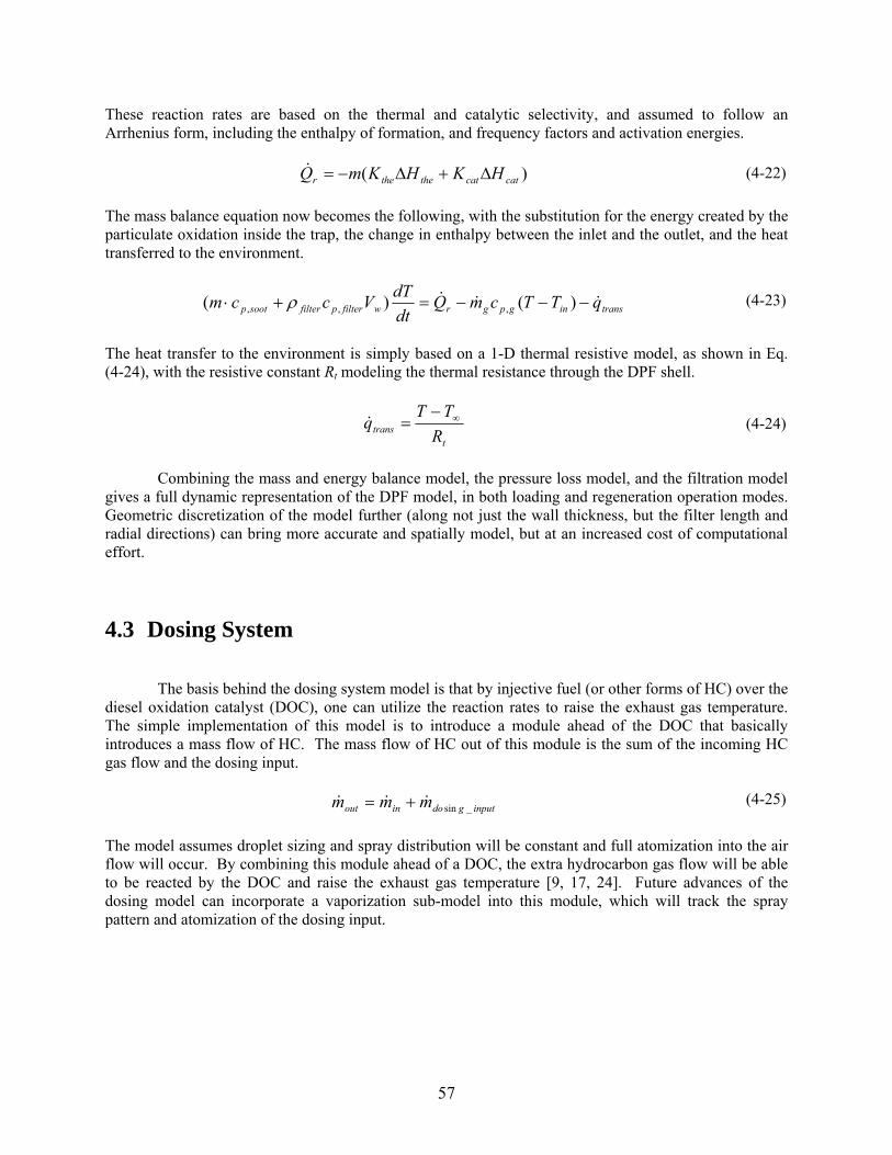
These reaction rates are based on the thermal and catalytic selectivity, and assumed to follow an Arrhenius form, including the enthalpy of formation, and frequency factors and activation energies.
(4-22) )( catcatthethe HKHKm ∆+∆−=rQ& The mass balance equation now becomes the following, with the substitution for the energy created by the particulate oxidation inside the trap, the change in enthalpy between the inlet and the outlet, and the heat transferred to the environment.
transingpgrwfilterpfiltersootp qTTcmQdtdTVcc &&& −−−=+ )() ,,, ρm ⋅( (4-23)
The heat transfer to the environment is simply based on a 1-D thermal resistive model, as shown in Eq. (4-24), with the resistive constant Rt modeling the thermal resistance through the DPF shell.
tRTT ∞−
=transq&
outm&
(4-24)
Combining the mass and energy balance model, the pressure loss model, and the filtration model
gives a full dynamic representation of the DPF model, in both loading and regeneration operation modes. Geometric discretization of the model further (along not just the wall thickness, but the filter length and radial directions) can bring more accurate and spatially model, but at an increased cost of computational effort.
4.3 Dosing System
The basis behind the dosing system model is that by injective fuel (or other forms of HC) over the diesel oxidation catalyst (DOC), one can utilize the reaction rates to raise the exhaust gas temperature. The simple implementation of this model is to introduce a module ahead of the DOC that basically introduces a mass flow of HC. The mass flow of HC out of this module is the sum of the incoming HC gas flow and the dosing input.
(4-25) inputgdoin mm _sin&& +=
The model assumes droplet sizing and spray distribution will be constant and full atomization into the air flow will occur. By combining this module ahead of a DOC, the extra hydrocarbon gas flow will be able to be reacted by the DOC and raise the exhaust gas temperature [9, 17, 24]. Future advances of the dosing model can incorporate a vaporization sub-model into this module, which will track the spray pattern and atomization of the dosing input.
57
4.4 Heater/Combustor System
A heater/combustor system is used, conceptually, to raise the exhaust gas temperature for filter regeneration purposes. These systems are considered self-contained, combustion systems that utilize the exhaust gas air (which is rich in oxygen content, since diesel exhaust is generally very lean), a spark plug, and fuel spray input to create a combustion process that will raise the exhaust gas temperature.
The difficulty in actually developing a system of this nature is the ability to control the
combustion accurately with the wide range of oxygen concentration and complex flow pattern of air in an exhaust pipe environment, as well as controlling the appropriate spark characteristics. Also, reliability and longevity of the components is a practical concern for such an application.
However difficult the practical concerns are, simple modeling of this system can be done by using
an ideal gas model and heat engine. A 0-D, linear, lumped parameter model is assumed, with no fluid flow or dimensional effects. The increase in air temperature can be approximated by the heating value of the fuel, the air/fuel mass flow ratios, the heat capacity of air, and an efficiency parameter.
airgasex
heatingHCinHCgasex cpm
LHVm⋅
T⋅⋅
=_
__ &
&∆
η (4-26)
The new exhaust gas temperature is simply the sum of the temperature coming into the module, the change in temperature from combustion, and any other thermal effects.
gasexingasout TT ___gasT ∆+= (4-27)
One important aspect with respect to emissions is the hydrocarbon slip past a combustor. In general, most combustors are not 100% efficient, whereby the hydrocarbon is completely burned. This effectively increases the hydrocarbon emissions past the combustor. A simple efficiency parameter is implemented in the model to account for this effect.
(4-28) inHCheatingemisHCoutHC mm ___ )1( &&m& η−+=
The efficiency parameter is the same as used in the temperature increase equation above. This efficiency parameter can be estimated to a first order approximation, generally from empirical data.
4.5 Lean NOx Trap (LNT)
A good understanding of the fundamental physical basis of how a NOx trap works, particularly a
lean NOx trap, is reasonably well known [18, 22, 23, 35, 38, 43]. A full one dimensional partial differential equation based description of the basic chemical and physical phenomena can be taken from prior work by Aimard et al [22]. However, a simpler, phenomenological based model can be implemented for the lean NOx trap. Lean burn engines (lean burn gasoline or diesel engines) typically utilize NOx traps to reduce emissions. When the engine is running with a lean air-fuel mixture (or rich in O2), the NO in the exhaust gas entering an LNT is catalytically oxidized to NO2. The NO2 is then stored
58

in a nearby cell site (usually composed of alkali metal or alkaline earth material) as a nitrate (in the example below barium nitrate). During times of rich exhaust mixture, the stored NO2 is released and catalytically reduced by the reductants of CO, H2, and HC to form H20, CO2, N2, and H2.
Figure 4-5: Storage and Purging of LNT (image courtesy [22])
These two phases (shown in Figure 4-5) of a lean NOx trap are known as the storage and purge
phases. The mechanisms by which these processes work is complex, but can be approximated for the purposes of a system model in a phenomenological, control oriented, lumped parameter model. NOx emission levels can be controlled by properly managing the purging and storing mechanisms, via lean and richer periods, or via fuel injection in the exhaust stream. In effect, unless there is passive triggering via engine air-fuel mixture modulation, there needs to be active triggering of the LNT to purge.
The major criteria that affect the operation of the LNT are its temperature, space velocity, NOx
concentration, the availability of storage sites, and the air-fuel ratio. These variables affect the behavior of the storage capacity, storage efficiency, and NOx conversion efficiency.
In summary, the mass flows of NOx out of the trap can be approximated by the storage efficiency during the storage phase (ηs), mass flow of NOx into the trap, mass flow released from the sites, and the conversion efficiency during the purging phase (ηc).
)1()1( ,,, creleasedNOxinNOxsout mmNOxm ηη −⋅+⋅−= &&& (4-29)
The storage dynamics of the LNT are derived from the basic chemistry of the following:
NO + ½ O2 NO2
BaCO3 + 2NO2 + ½ O2 Ba(NO3)2 + CO2 What the model does, however, is simplify the storage dynamics into two aspects, that of storage capacity and the efficiency as a function of temperatures. The storage capacity is primarily a function of trap temperature, with the maximum capacity set by geometric and catalyst formulation constraints. A typical first order approximation is shown in Figure 4-6.
59
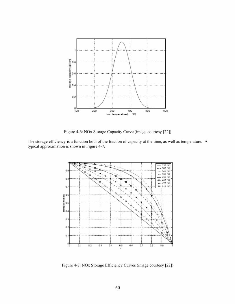
Figure 4-6: NOx Storage Capacity Curve (image courtesy [22])
The storage efficiency is a function both of the fraction of capacity at the time, as well as temperature. A typical approximation is shown in Figure 4-7.
Figure 4-7: NOx Storage Efficiency Curves (image courtesy [22])
60
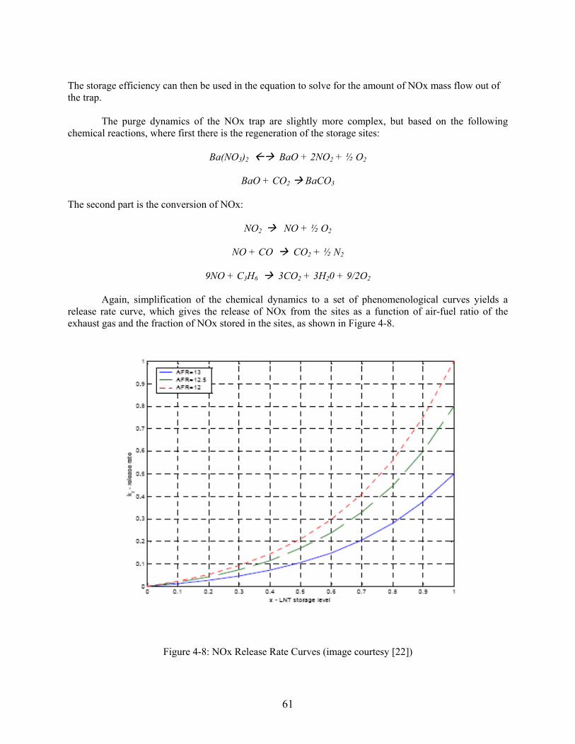
The storage efficiency can then be used in the equation to solve for the amount of NOx mass flow out of the trap.
The purge dynamics of the NOx trap are slightly more complex, but based on the following chemical reactions, where first there is the regeneration of the storage sites:
Ba(NO3)2 BaO + 2NO2 + ½ O2
BaO + CO2 BaCO3
The second part is the conversion of NOx:
NO2 NO + ½ O2
NO + CO CO2 + ½ N2
9NO + C3H6 3CO2 + 3H20 + 9/2O2 Again, simplification of the chemical dynamics to a set of phenomenological curves yields a
release rate curve, which gives the release of NOx from the sites as a function of air-fuel ratio of the exhaust gas and the fraction of NOx stored in the sites, as shown in Figure 4-8.
Figure 4-8: NOx Release Rate Curves (image courtesy [22])
61
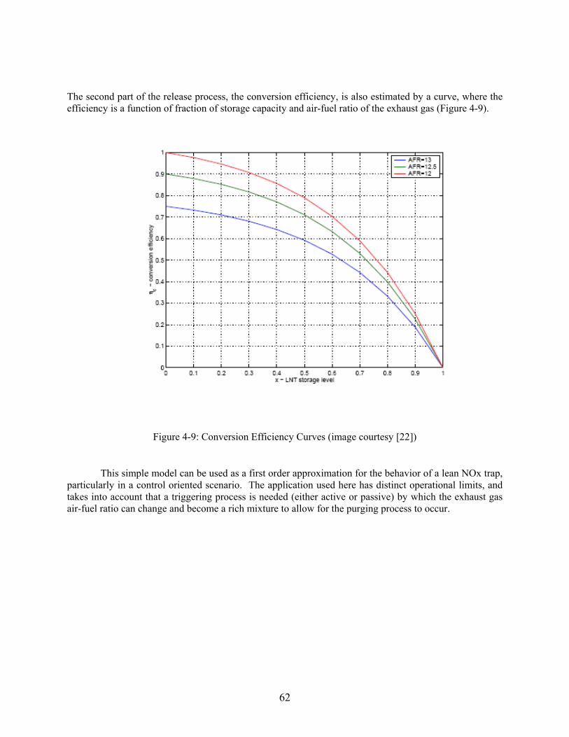
The second part of the release process, the conversion efficiency, is also estimated by a curve, where the efficiency is a function of fraction of storage capacity and air-fuel ratio of the exhaust gas (Figure 4-9).
Figure 4-9: Conversion Efficiency Curves (image courtesy [22])
This simple model can be used as a first order approximation for the behavior of a lean NOx trap, particularly in a control oriented scenario. The application used here has distinct operational limits, and takes into account that a triggering process is needed (either active or passive) by which the exhaust gas air-fuel ratio can change and become a rich mixture to allow for the purging process to occur.
62

Chapter 5 . Single Component Sizing Optimization: DOC Case Example
5.1 Introduction
The first step to validating the modeling and simulation tool as well as the methodology concept
presented in the prior chapters is to begin with a simple example and expand on it to make a representative complex system. This example should be able to evaluate the model in the multi-disciplinary, multi-objective, system wide methodology. One of the end goals is to be able to obtain the relative performance of different system architectures and/or system designs in objective space given a certain engine/vehicle, operating conditions, and other constraints and limitations.
The case example begins with a DOC (diesel oxidation catalyst), which consists of a monolith honeycomb substrate coated with platinum group metal catalyst, packaged within a (usually) stainless steel container. Generally, the chemical processes are modeled from first principles or by a conversion efficiency table, where the conversion efficiency percentage reduction of the emissions species is a function of temperature (either gas or catalyst) and potentially of catalyst substrate properties, and is described in Chapter 4, Section 4.1, and Appendix A with more detail.
The engine/vehicle combination used for the analysis is a small car chassis with a Volkswagen
1.9 liter Direct Injection Diesel engine. The engine data and settings were run in ADVISOR 2002 [1], a vehicle simulator that can operate a engine/vehicle combination under a variety of drive conditions. The drive cycle used for the analysis is the US City FTP (Federal Test Procedure). The emissions data from the engine is collected from ADVISOR and used as an input to the exhaust system modeling and simulation tool.
The optimization objective was to size the catalyst in such a manner as to maximize its emission performance (i.e. maximize the reduction of pollutant emissions). Further work included adding in other drive cycles and performing a design space exploration of catalyst formulations – a typical engineering trade-off study.
63

Objectives of the DOC Sizing Case:
• Validate modeling capability by simulating a complete vehicle drive cycle and engine configuration through the exhaust system model.
• Implement optimization using gradient and heuristics algorithms, and multi-objective optimization methods. Optimization results should validate typically known behavior.
• Design space exploration of catalyst formulation. The basic modeling assumptions of the DOC can be seen in Chapter 4 and the relevant Appendix.
The geometric variables are based on the ability of the designers to physically build a particular exhaust system to fit a particular chassis. Figure 5-1 shows an overview of the physical model with respect to the engine (see also Figure 1-5), and Figure 5-2 shows the detailed mapping of the design variables with the physical implementation of the catalyst design.
Engine DOC
Manifold Downpipe
Figure 5-1: DOC Case Study Architecture The initial simulation also includes a down-pipe between the engine and the catalyst. This down-pipe is treated as a standard pipe flow with heat dissipation. The geometric sizing variables for the down-pipe are length, radius, and thickness.
5.2 Design and Performance Objectives
The initial performance objective function is to minimize the tailpipe emissions of the vehicle by incorporating all of the regulated emissions species into the objective function, shown in Equation (5-1).
Min ]____[ emissionsPMemissionsNOxemissionsCOemissionsHCf +++= (5-1)
In order to fit a single objective, the function is a weighted sum of the normalized emission species. Normalizing the emissions results allows us to directly compare the emissions values, without having to examine the difference in magnitudes of the actual values of exhaust species emissions. In order to normalize the effects of each emissions type, the output of the exhaust system emission species will be divided by a regulation limit (see Table 5-1). The values of the normalized emissions contributions will lie between 0 and 1; with any value over 1 effectively making that design unfeasible (because it will not meet emissions regulations). This can give the optimizer a direct comparison to evaluate the designs of the exhaust system. The regulations limit allow a certain amount of emissions per mile traveled, usually given in grams per mile. These emissions are measured under the US Federal Test Procedure protocol, which puts a vehicle through a specified speed/load drive cycle (Example shown in
64

Figure 5-3). For this case the emission from light duty vehicle regulations, US EPA Tier 1 Emission Standards for Passenger Cars and Light Duty Trucks, were used (Table 5-1), fully implemented from 1997 through 2003 in order to best match the engine model used in ADVISOR.
Table 5-1: Emission Regulation, US Tier 1 Emissions Regulation HC 0.41 g/mileCO 3.4 g/mileNOx 1.0 g/milePM 0.08 g/mile
The single objective function is thus transformed into Eq. (5-2).
Min ][ReReReRe
⎟⎟⎠
⎞⎜⎜⎝
⎛⋅+⎟
⎟⎠
⎞⎜⎜⎝
⎛⋅+⎟
⎟⎠
⎞⎜⎜⎝
⎛⋅+⎟
⎟⎠
⎞⎜⎜⎝
⎛⋅=
g
emisPM
g
emisNOx
g
emisCO
g
emisHC PM
PMwNOxNOxw
COCOw
HCHCwf (5-2)
The sum of the individual weights were constrained, Eq. (5-3), and for the following set of tests, the weights were equal to 0.25.
PMNOxCOHC wwww ====0 25. (5-3)
5.3 Design Variables
Although many variables can be used within a DOC, only a small set were defined as independent variables, with the majority of these variables used for geometric sizing of the catalyst for design purposes. Figure 5-1 shows an overview of the physical model with respect to the engine, and Figure 5-2 [2] shows the detailed mapping of the design variables to the physical implementation of the catalyst design.
The initial simulation also includes a down-pipe between the engine and the catalyst, with the geometric sizing variables for the down-pipe are length, radius, and thickness. The constraints of the system are built into the model by bounding the design variables to within a certain range. These ranges can be set within iSight, and are up to the designer to specify, depending on their constraints within the entire vehicle system. The design variables in the design vector are defined in Section 5.3.1.
65
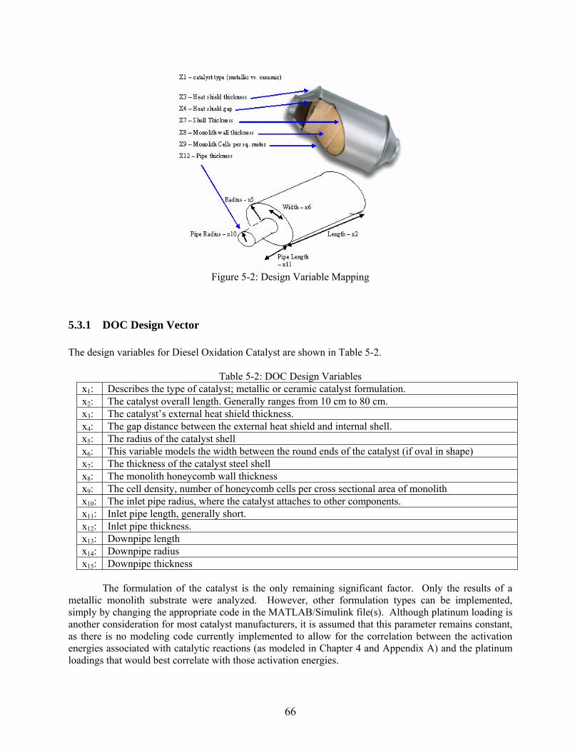
Figure 5-2: Design Variable Mapping
5.3.1 DOC Design Vector The design variables for Diesel Oxidation Catalyst are shown in Table 5-2.
Table 5-2: DOC Design Variables x1: Describes the type of catalyst; metallic or ceramic catalyst formulation. x2: The catalyst overall length. Generally ranges from 10 cm to 80 cm. x3: The catalyst’s external heat shield thickness. x4: The gap distance between the external heat shield and internal shell. x5: The radius of the catalyst shell x6: This variable models the width between the round ends of the catalyst (if oval in shape) x7: The thickness of the catalyst steel shell x8: The monolith honeycomb wall thickness x9: The cell density, number of honeycomb cells per cross sectional area of monolith x10: The inlet pipe radius, where the catalyst attaches to other components. x11: Inlet pipe length, generally short. x12: Inlet pipe thickness. x13: Downpipe length x14: Downpipe radius x15: Downpipe thickness
The formulation of the catalyst is the only remaining significant factor. Only the results of a
metallic monolith substrate were analyzed. However, other formulation types can be implemented, simply by changing the appropriate code in the MATLAB/Simulink file(s). Although platinum loading is another consideration for most catalyst manufacturers, it is assumed that this parameter remains constant, as there is no modeling code currently implemented to allow for the correlation between the activation energies associated with catalytic reactions (as modeled in Chapter 4 and Appendix A) and the platinum loadings that would best correlate with those activation energies.
66

5.4 Design Constraints
The sizing and material constraints are built into the design variable bounds. The designers and
users of the models have limited materials to choose from, and are thus limited in the availability and sizes of these materials. The bounds of the design variables are effectively constraints on the problem. The formulation of the catalyst is the only remaining significant factor. For this example, only the results of a metallic monolith substrate were analyzed with a specific cell density and wall thickness formulation. The upper and lower bounds can be seen in Table 5-10.
5.5 Simulation Parameters and Validation and Optimization Set-up
A commercial optimization program, iSight, was used to optimize the DOC and downpipe system
and interfaced with the Matlab/Simulink simulation code. Each iteration of simulation takes approximately 2 seconds of CPU time. A flow chart diagram of the optimization loop and simulation is described in Chapter 3 and shown in Figure 3-7. The significant simulation parameters used within the DOC model are shown in Table 5-3:
Table 5-3: Simulation Parameters Ambient and initial temperatures 30 deg C Densities for mass calculations, typical steel 8000 kg/m3
Poiseuille Number 15 Fluid Viscosity of Air 2.5 Ns/m2
Density of Air 1.225 kg/m3
Specific Heat of Steel 460 J/kgK
The drive cycle from which the engine data was derived from is a standard US Federal Test Procedure. An example vehicle speed over cycle time plot is shown in Figure 5-3 [1]. It is important to note that the US FTP cycle has a section of time where the vehicle is turned off, and then restarted. This is used to simulate a warm start procedure, in addition to the cold start procedure at the beginning of the cycle.
67

Figure 5-3: FTP Vehicle Speed Trace
5.6 Design Space Results for Single Objective Optimization using Gradient Based Algorithm
The initial starting design point was the mid-range values for all the design variables (see Table 5-4). Other initial design vectors were used to investigate the behavior of gradient based optimization and to verify the global optimum. Afterwards, a sensitivity analysis was performed over the design variables.
Table 5-4: Initial Design Variable Values Design Variable Value Lower Bound Upper Bound
x1: Catalyst Type Metallic N/A N/A x2: Catalyst overall length. 50.0 cm 20.0 cm 70.0 cm x3: Catalyst’s external heat shield thickness. 1.5 mm 1.2 mm 1.8 mm x4: Gap distance between external heat shield and internal shell. 1.0 cm 1.0 mm 2.5 cm x5: Radius of the catalyst shell 5.0 cm 1.5 cm 7.0 cm x6: Catalyst width 2.5 cm 0.0 cm 5.0 cm x7: Thickness of the catalyst steel shell 1.5 mm 1.2 mm 1.8 mm x8: Monolith honeycomb wall thickness 0.05 mm 0.025 mm 0.1 mm x9: Cell density 300 cpsi 200 cpsi 400 cpsi x10: Inlet pipe radius 4.0 cm 1.5 cm 7.0 cm x11: Inlet pipe length 4.0 cm 1.0 cm 5.0 cm x12: Inlet pipe thickness 1.5 mm 1.2 mm 1.8 mm x13: Downpipe length 50.0 cm 1.0 cm 100.0 cm x14: Downpipe radius 4.0 cm 1.5 cm 7.0 cm x15: Downpipe thickness 1.5 mm 1.2 mm 1.8 mm
68
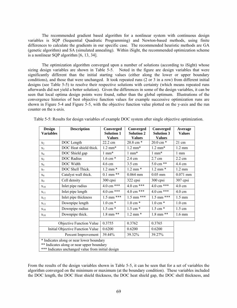
The recommended gradient based algorithm for a nonlinear system with continuous design
variables is SQP (Sequential Quadratic Programming) and Newton-based methods, using finite differences to calculate the gradients in our specific case. The recommended heuristic methods are GA (genetic algorithm) and SA (simulated annealing). Within iSight, the recommended optimization scheme is a nonlinear SQP algorithm [6, 13, 34].
The optimization algorithm converged upon a number of solutions (according to iSight) whose sizing design variables are shown in Table 5-5. Noted in the figure are design variables that were significantly different than the initial starting values (either along the lower or upper boundary conditions), and those that were unchanged. It took repeated runs (2 or 3 in a row) from different initial designs (see Table 5-5) to resolve their respective solutions with certainty (which means repeated runs afterwards did not yield a better solution). Given the differences in some of the design variables, it can be seen that local optima design points were found, rather than the global optimum. Illustrations of the convergence histories of best objective function values for example successive optimization runs are shown in Figure 5-4 and Figure 5-5, with the objective function value plotted on the y-axis and the run counter on the x-axis.
Table 5-5: Results for design variables of example DOC system after single objective optimization.
Design Variables
Description Converged Solution 1
Values
Converged Solution 2
Values
Converged Solution 3
Values
Average Values
x2 DOC Length 22.2 cm 20.8 cm * 20.0 cm * 21 cm x3 DOC Heat shield thick. 1.2 mm* 1.2 mm* 1.2 mm* 1.2 mm x4 DOC Shield gap 1 mm* 1 mm* 1 mm* 1 mm x5 DOC Radius 1.6 cm * 2.4 cm 2.7 cm 2.2 cm x6 DOC Width 4.6 cm 3.5 cm 5.0 cm ** 4.4 cm x7 DOC Shell Thick. 1.2 mm * 1.2 mm * 1.2 mm * 1.2 mm x8 Catalyst wall thick. 0.1 mm ** 0.064 mm 0.05 mm 0.071 mm x9 Cell density 300 cpsi 322 cpsi 300 cpsi 307 cpsi x10 Inlet pipe radius 4.0 cm *** 4.0 cm *** 4.0 cm *** 4.0 cm x11 Inlet pipe length 4.0 cm *** 4.0 cm *** 4.0 cm *** 4.0 cm x12 Inlet pipe thickness 1.5 mm *** 1.5 mm *** 1.5 mm *** 1.5 mm x13 Downpipe length 1.0 cm * 1.0 cm * 1.0 cm * 1.0 cm x10 Downpipe radius 1.5 cm * 1.5 cm * 1.5 cm * 1.5 cm x10 Downpipe thick. 1.8 mm ** 1.2 mm * 1.8 mm ** 1.6 mm
Objective Function Value 0.3755 0.3762 0.3765 Initial Objective Function Value 0.6200 0.6200 0.6200
Percent Improvement 39.44% 39.32% 39.27% * Indicates along or near lower boundary ** Indicates along or near upper boundary *** Indicates unchanged value from initial design
From the results of the design variables shown in Table 5-5, it can be seen that for a set of variables the algorithm converged on the minimum or maximum (at the boundary condition). These variables included the DOC length, the DOC Heat shield thickness, the DOC heat shield gap, the DOC shell thickness, and
69
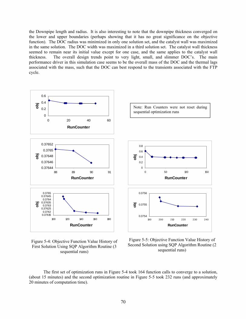
the Downpipe length and radius. It is also interesting to note that the downpipe thickness converged on the lower and upper boundaries (perhaps showing that it has no great significance on the objective function). The DOC radius was minimized in only one solution set, and the catalyst wall was maximized in the same solution. The DOC width was maximized in a third solution set. The catalyst wall thickness seemed to remain near its initial value except for one case, and the same applies to the catalyst wall thickness. The overall design trends point to very light, small, and slimmer DOC’s. The main performance driver in this simulation case seems to be the overall mass of the DOC and the thermal lags associated with the mass, such that the DOC can best respond to the transients associated with the FTP cycle.
0
0.2
0.4
0.6
0 20 40 60
RunCounter
obj
0.37644
0.37646
0.37648
0.3765
0.37652
88 89 90 91
RunCounter
obj
0.376150.3762
0.376250.3763
0.376350.3764
0.376450.3765
100 120 140 160 180
RunCounter
obj
0
0.2
0.4
0.6
0.8
0 50 100 150
RunCounter
obj
0.3754
0.3755
0.3756
190 200 210 220 230 240
RunCounter
obj
Note: Run Counters were not reset during sequential optimization runs
Figure 5-5: Objective Function Value History of
Second Solution using SQP Algorithm Routine (2 sequential runs)
Figure 5-4: Objective Function Value History of First Solution Using SQP Algorithm Routine (3
sequential runs) The first set of optimization runs in Figure 5-4 took 164 function calls to converge to a solution,
(about 15 minutes) and the second optimization routine in Figure 5-5 took 232 runs (and approximately 20 minutes of computation time).
70
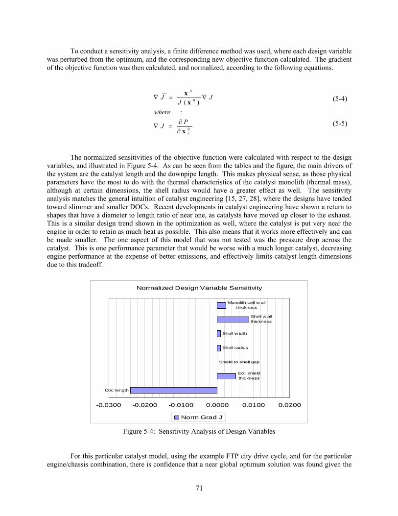
To conduct a sensitivity analysis, a finite difference method was used, where each design variable was per
5-
turbed from the optimum, and the corresponding new objective function calculated. The gradient of the objective function was then calculated, and normalized, according to the following equations.
4
0
0
0
:)(
i
P
JJ
x
xx
∂∂
=J
where
J
∇
=∇
The normalized sensitivities of the objective function were calculated with respect to thevariable
For this particular catalyst model, using the example FTP city drive cycle, and for the paengine/chassis combination, there is confidence that a near global optimum solution was found gi
∇
s, and illustrated in Figure 5-4. As can be seen from the tables and the figure, the main drthe system are the catalyst length and the downpipe length. This makes physical sense, as those pparameters have the most to do with the thermal characteristics of the catalyst monolith (thermalalthough at certain dimensions, the shell radius would have a greater effect as well. The senanalysis matches the general intuition of catalyst engineering [15, 27, 28], where the designs havetoward slimmer and smaller DOCs. Recent developments in catalyst engineering have shown a rshapes that have a diameter to length ratio of near one, as catalysts have moved up closer to the eThis is a similar design trend shown in the optimization as well, where the catalyst is put very nengine in order to retain as much heat as possible. This also means that it works more effectively be made smaller. The one aspect of this model that was not tested was the pressure drop acrcatalyst. This is one performance parameter that would be worse with a much longer catalyst, decengine performance at the expense of better emissions, and effectively limits catalyst length dimdue to this tradeoff.
Figure 5-4: Sensitivity Analysis of Design Variables
Normalized Design Variable Sensitivity
Doc length
Ext. shield thickness
Shield to shell gap
Shell radius
Shell w idth
Shell w all thickness
Monolith cell w all thickness
-0.0300 -0.0200 -0.0100 0.0000 0.0100 0.0200
Norm Grad J
71
(5-4)
-5)
(5
design
rticular ven the
ivers of hysical mass), sitivity tended eturn to xhaust. ear the
and can oss the reasing ensions
single o
.7 Transient and Steady State Design of Experiment Simulation
Upon review of the initial optimization results, it was decided to further investigate the catalyst formulation in detail and include other transient and steady state cycles to test other operating conditions, using th
bjective of this comparative analysis was to resolve the general behavior of emissions erformance given the mass of the monolith. The mass of the DOC monolith is vital in determining the
thermal
bjective function as defined, and the various constraints and design parameters. The reason for this confidence is that multiple simulations from different initial design points did not result in an improved design, but instead brought results nearer to this solution. Similarly, the results of the heuristic (GA) algorithm corroborate those found with the gradient based method, as the GA results are in a very similar design and objective space as shown in Section 5.8.
5for Different Oxidation Catalyst Formulations
e same small diesel engine baseline [1] (Volkswagen 1.9 liter). A typical development problem for engineers after optimizing the layout (as in Section 5.6) would be to resolve the catalyst formulation, with regards to cell density and monolith wall thickness, given a certain geometric size, optimized over a variety of different operating points. Using the DOC model previously described and implemented within the modeling framework, a straightforward design of experiments [13] was used to investigate the thermal mass behavior for the two design variables (monolith wall thickness and cell density) that define the catalyst monolith and directly impact cost and manufacturing. Note, that mid-range values for the other DOC design variables were used. The downpipe design variables were set to the optimal values found in Section 5.6.
The op
behavior, and thus operating temperature of the catalyst. The mass of the catalyst monolith was defined primarily as a function of two variables, the wall thickness and cell density, as shown in figure, and keeping the catalyst length and radius constant (thus keeping volume constant).
72

DOC Cell Wall Thickness and Cell Density
Unit Cell (or channel)
Cell wall thickness
Cell Density: Number of cells per square inch
Figure 5-5: DOC Cell Wall Thickness and Cell Density
The initial results of the Design of Experiments (full factorial, as shown in Table 5-6 and Table 5-7) found what appeared to be areas of the design space in terms of mass of the catalyst (with certain combinations of wall thickness and cell density) that offered the best emission performance level for specific gas species. The DOE study show a few key points also corroborated by other tests [15, 27, 29, 30].
• Monolith thermal mass greatly affects the emission performance of the DOC.
• The general trend for better emissions is lowering thermal mass through use of less cell density and thinner wall thickness.
• The transient cycle simulations showed that optimal performance of emissions resided within the design space (as given by typical catalyst formulation geometries), albeit close to the boundary. Increasing or decreasing thermal mass from that point led to worse performance, although the vast majority of the design space indicated reducing thermal mass would improve performance.
73

• There is a distinct trade-off between light thermal mass that allows for quick warm-up and heavy thermal mass that allows for temperature to remain high during transients. This was evident in the temperature tracking, and the resultant performance of the catalyst due to its temperature. Since pure steady state conditions are not necessarily representative of reality, the results for transient cases should take greater weight. These would indicate that less thermal mass for less lag would benefit emissions in general.
It can be seen (from Table 5-6) that the overall objective function as previously defined in Section
5.2 is lower with less monolith mass in the steady state case. This can be explained by the long warm-up time associated with very heavy monoliths, and the resulting poor emission performance. Note, that the overall objective function value between the steady state case and transient case is different due to the steady state operating points. These operating points produce significantly more emissions than the transient case over the same amount of time.
The transient case incorporates the interplay between warm-up time, and heat capacity of the monolith’s ability to retain heat in cooler exhaust gas temperatures. Table 5-7 illustrates that within the typical configurations of 200-400 CPSI cell densities and 1 mil to 6 mil thickness walls, it is evident that the lowest thermal mass performed the best in terms of emissions output. However, experimenting with reducing the mass further (in this case by reducing cell density to 1/3, and then 1/6 of the lowest typical cell density), the performance worsened. A physical explanation for this was not clearly evident given the steady state conditions the engine operation, but it could be seen that worse HC and CO emissions significantly contributed to the worse objective function performance. The overall objective function has a minimum value of just under 0.40 at around 500 g mass (given the other geometric design variables remaining constant).
An important aspect in this trade-off design space exploration analysis is that each species’ optimal performance is at different catalyst masses. Each species’ performance response surface also has different gradients. In particular, it appears that HC and CO emissions are best at values about 500 grams. NOx emissions is a non-convex result, where very low NOx emissions were had for low masses (under 300 g) and higher masses (around 1000 g), but performed worse in between and at the extremities. Particulate matter performance was clearly better with lower masses.
74

Table 5-6 Steady state test case emissions results of typical catalyst configurations
mon cell wall thk 200 CPSI 400 CPSIHC [g] 8.6125 8.7046CO [g] 9.0546 9.3126Nox [g] 2.3822 2.4501PM [g] 0.4431 0.453Objective 0.7152 0.7263mon mass 519 g 734 gvolume 2.33 liters 2.33 litersCS cells 1806 3613CSA 9.03 sq in 9.03 sq in
HC [g] 8.7558 8.7919CO [g] 9.4712 9.6129Nox [g] 2.5245 2.5786PM [g] 0.4606 0.4678Objective 0.734 0.7402mon mass 1038 g 1468 gvolume 2.33 liters 2.33 litersCS cells 1806 3613CSA 9.03 sq in 9.031 sq in
HC [g] 9.095 9.4336CO [g] 10.7442 11.9729Nox [g] 2.7669 2.9259PM [g] 0.5003 0.53Objective 0.7779 0.8168mon mass 3113 g 4404 gvolume 2.33 liters 2.33 litersCS cells 1806 3613CSA 9.031 sq in 9.031 sq in
Steady State
1 mil
6 mil
cell density
2 mil
Table 5-7 Transient test case emissions results for typical catalyst configurations and low cell
mon cell wall thk 33 CPSI 70 CPSI 200 CPSI 400 CPSIHC [g] 2.9913 2.897 2.8463 2.9822CO [g] 10.7892 10.3455 10.0085 10.0528Nox [g] 4.1098 4.144 4.1348 4.1192PM [g] 0.2552 0.2606 0.272 0.2832Objective 0.4023 0.3964 0.3944 0.4mon mass 209 g 309 g 519 g 734 gvolume 2.33 liters 2.33 liters 2.33 liters 2.33 litersCS cells 291 640 1806 3613CSA 9.03 sq in 9.03 sq in 9.03 sq in 9.03 sq in
HC [g] 2.9961 3.2658CO [g] 10.2787 10.9635Nox [g] 4.1158 4.1626PM [g] 0.2963 0.3192Objective 0.4109 0.4379mon mass 1038 g 1468 gvolume 2.33 liters 2.33 litersCS cells 1806 3613CSA 9.03 sq in 9.031 sq in
HC [g] 4.0255 4.2781CO [g] 12.7871 13.2351Nox [g] 4.4813 4.5795PM [g] 0.374 0.3921Objective 0.5147 0.539mon mass 3113 g 4404 gvolume 2.33 liters 2.33 litersCS cells 1806 3613CSA 9.031 sq in 9.031 sq in
1 mil
2 mil
6 mil
cell density
Transient (FTP)
75

Table 5-8: Legend for Table 5-6 and Table 5-7 Variable Description
Mon mass DOC monolith mass CS cells No. of cells in DOC cross section CSA Cross sectional area of DOC HC Total grams of HC emissions CO Total grams of CO emissions NOx Total grams of CO emissions PM Total grams of CO emissions
For differing cycles, there is definite interplay between the requirements of a quick light off (warm up) of the catalyst and the necessity to hold heat during transient states. This optimum performance point is most likely different for each cycle and engine configuration. However, the ability of the modeling and simulation tool to illustrate this, as well as offering the capability to adjust the architecture and detailed design of the exhaust system, illustrates how valuable the information from the models can be for engineers.
The results from the catalyst mass analysis also show that the response surface for each emissions
species can be nonlinear, depending on the application and the drive cycle used. This shows that when dealing with multi-objective analysis, it is important to initially obtain a coarse, global response surface using heuristics, so that potential optima in the objective space areas are searched. Additionally, it is important to examine the design space and how that correlates to the optima in the objective space. Once this is complete, then a finer grain optimization can be done in the objective space areas that show potential for local optima. The results of those can then be compared for development purposes.
5.8 Heuristic Algorithm Results for Single Objective Optimization
A Genetic Algorithm was used in the heuristic optimization case due to its comparability between various stand alone optimization programs, and that it allows for the ability to use both discrete and continuous variables. A GA is also useful in being able to be used to parse through the design space without getting stuck in local optima. Given the highly non-linear nature of the design problem, and the possibility of having discrete variables (such as catalyst formulation type driving other parameters), starting with a GA was preferable in order to be able to match and correlate results. The expected results from the GA are as robust as those running multiple gradient based algorithms in the case of the DOC. However, when running a case with a large number of variables that can be highly nonlinear, a GA can be used to help pinpoint the potential areas for local optima.
In the DOC case, the Genetic Algorithm took 1015 runs, and approximately 100 minutes to complete. The initial design vector of midrange values was used as a seed (the same as in Section 5.6). The techniques used in this optimization run was a first step through a multi-island genetic algorithm, and then a refinement using Sequential Quadratic Programming (NLPQL). The results of the GA showed that the best design found did not improve over that found using the gradient based method alone. However, the GA found the optimal solution in one optimization routine, whereas the gradient method required multiple optimization runs to be certain of the global optimal solution. Running the GA from 3 different initial points (seeds) all resulted in the same optimized objective value.
76
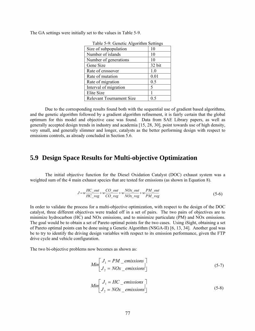
The GA settings were initially set to the values in Table 5-9.
Table 5-9: Genetic Algorithm Settings Size of subpopulation 10 Number of islands 10 Number of generations 10 Gene Size 32 bit Rate of crossover 1.0 Rate of mutation 0.01 Rate of migration 0.5 Interval of migration 5 Elite Size 1 Relevant Tournament Size 0.5
Due to the corresponding results found both with the sequential use of gradient based algorithms,
and the genetic algorithm followed by a gradient algorithm refinement, it is fairly certain that the global optimum for this model and objective case was found. Data from SAE Library papers, as well as generally accepted design trends in industry and academia [15, 28, 30], point towards use of high density, very small, and generally slimmer and longer, catalysts as the better performing design with respect to emissions controls, as already concluded in Section 5.6.
5.9 Design Space Results for Multi-objective Optimization
The initial objective function for the Diesel Oxidation Catalyst (DOC) exhaust system was a weighted sum of the 4 main exhaust species that are tested for emissions (as shown in Equation 8).
regPMoutPMw
regNOxoutNOxw
regCOoutCOw
regHCoutHC
__
__
__
__
+++wJ =
Min
Min
(5-6)
In order to validate the process for a multi-objective optimization, with respect to the design of the DOC catalyst, three different objectives were traded off in a set of pairs. The two pairs of objectives are to minimize hydrocarbon (HC) and NOx emissions, and to minimize particulate (PM) and NOx emissions. The goal would be to obtain a set of Pareto optimal points for the two cases. Using iSight, obtaining a set of Pareto optimal points can be done using a Genetic Algorithm (NSGA-II) [6, 13, 34]. Another goal was be to try to identify the driving design variables with respect to its emission performance, given the FTP drive cycle and vehicle configuration. The two bi-objective problems now becomes as shown as:
⎥⎦
⎤⎢⎣
⎡==
emissionsNOxJemissionsPMJ
__
2
1 (5-7)
⎥⎦
⎤⎢⎣
⎡==
emissionsNOxJemissionsHCJ
__
2
1 (5-8)
77
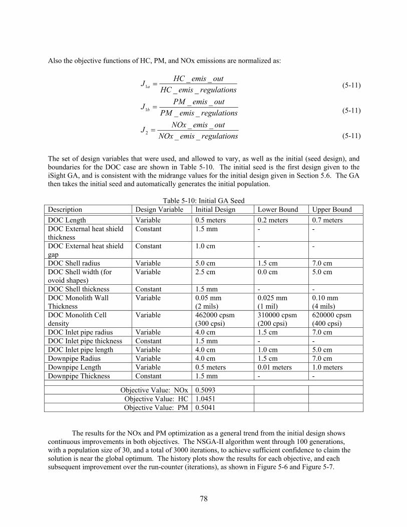
Also the objective functions of HC, PM, and NOx emissions are normalized as:
sregulationemisNOxoutemisNOx
sregulationemisPMoutemisPM
sregulationemisHCoutemisHC
____
____
____
=
=
=
J
J
J
b
a
2
1
1
(5-11) (5-11) (5-11)
The set of design variables that were used, and allowed to vary, as well as the initial (seed design), and boundaries for the DOC case are shown in Table 5-10. The initial seed is the first design given to the iSight GA, and is consistent with the midrange values for the initial design given in Section 5.6. The GA then takes the initial seed and automatically generates the initial population.
Table 5-10: Initial GA Seed Description Design Variable Initial Design Lower Bound Upper Bound
DOC Length Variable 0.5 meters 0.2 meters 0.7 meters DOC External heat shield thickness
Constant 1.5 mm - -
DOC External heat shield gap
Constant 1.0 cm - -
DOC Shell radius Variable 5.0 cm 1.5 cm 7.0 cm DOC Shell width (for ovoid shapes)
Variable 2.5 cm 0.0 cm 5.0 cm
DOC Shell thickness Constant 1.5 mm - - DOC Monolith Wall Thickness
Variable 0.05 mm (2 mils)
0.025 mm (1 mil)
0.10 mm (4 mils)
DOC Monolith Cell density
Variable 462000 cpsm (300 cpsi)
310000 cpsm (200 cpsi)
620000 cpsm (400 cpsi)
DOC Inlet pipe radius Variable 4.0 cm 1.5 cm 7.0 cm DOC Inlet pipe thickness Constant 1.5 mm - - DOC Inlet pipe length Variable 4.0 cm 1.0 cm 5.0 cm Downpipe Radius Variable 4.0 cm 1.5 cm 7.0 cm Downpipe Length Variable 0.5 meters 0.01 meters 1.0 meters Downpipe Thickness Constant 1.5 mm - -
Objective Value: NOx 0.5093 Objective Value: HC 1.0451 Objective Value: PM 0.5041
The results for the NOx and PM optimization as a general trend from the initial design shows continuous improvements in both objectives. The NSGA-II algorithm went through 100 generations, with a population size of 30, and a total of 3000 iterations, to achieve sufficient confidence to claim the solution is near the global optimum. The history plots show the results for each objective, and each subsequent improvement over the run-counter (iterations), as shown in Figure 5-6 and Figure 5-7.
78
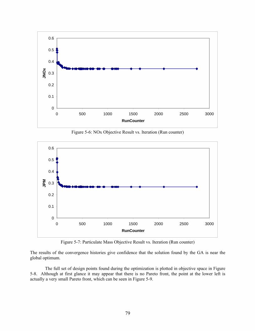
0
0.1
0.2
0.3
0.4
0.5
0.6
0 500 1000 1500 2000 2500 3000
RunCounter
JNO
x
Figure 5-6: NOx Objective Result vs. Iteration (Run counter)
0
0.1
0.2
0.3
0.4
0.5
0.6
0 500 1000 1500 2000 2500 3000
RunCounter
JPM
Figure 5-7: Particulate Mass Objective Result vs. Iteration (Run counter)
The results of the convergence histories give confidence that the solution found by the GA is near the global optimum.
The full set of design points found during the optimization is plotted in objective space in Figure 5-8. Although at first glance it may appear that there is no Pareto front, the point at the lower left is actually a very small Pareto front, which can be seen in Figure 5-9.
79
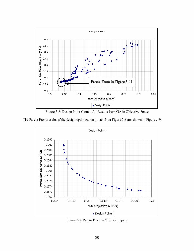
Design Points
0.2
0.25
0.3
0.35
0.4
0.45
0.5
0.55
0.6
0.3 0.35 0.4 0.45 0.5 0.55 0.6 0.65
NOx Objective (J NOx)
Par
ticul
ate
Mas
s O
bjec
tive
(J P
M)
Design Points
Pareto Front in Figure 5-11
Figure 5-8: Design Point Cloud. All Results from GA in Objective Space
The Pareto Front results of the design optimization points from Figure 5-8 are shown in Figure 5-9.
Design Points
0.267
0.2672
0.2674
0.2676
0.2678
0.268
0.2682
0.2684
0.2686
0.2688
0.269
0.2692
0.337 0.3375 0.338 0.3385 0.339 0.3395 0.34
NOx Objective (J NOx)
Parti
cula
te O
bjec
tive
(J P
M)
Design Points
Figure 5-9: Pareto Front in Objective Space
80
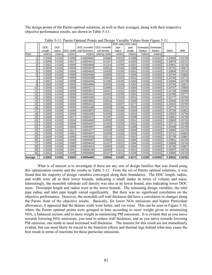
The design points of the Pareto optimal solutions, as well as their averages, along with their respective objective performance results, are shown in Table 5-11.
Table 5-11: Pareto Optimal Points and Design Variable Values from Figure 5-11
DOC Length
DOC radius DOC width
DOC monolith wall thickness
DOC monolith cell density
DOC inlet pipe
radius
DOC inlet pipe
lengthDownpipe
RadiusDownpipe
Radius JNOx JPMPoint meters meters meters meters cells/sq meter meters meters meters meters - -
1 0.2000 0.0150 0.0000 0.00005001 310685 0.0212 0.0289 0.0150 0.01001 0.33939 0.267282 0.2009 0.0150 0.0017 0.00004414 311027 0.0237 0.0292 0.0150 0.01000 0.33879 0.267413 0.2001 0.0150 0.0000 0.00004849 311314 0.0230 0.0251 0.0150 0.01002 0.33901 0.267334 0.2000 0.0150 0.0004 0.00003878 310012 0.0154 0.0283 0.0150 0.01000 0.33731 0.268715 0.2000 0.0150 0.0004 0.00004605 310035 0.0155 0.0261 0.0150 0.01000 0.33859 0.267436 0.2000 0.0150 0.0000 0.00004084 310083 0.0212 0.0284 0.0150 0.01000 0.33744 0.268267 0.2005 0.0150 0.0004 0.00004298 310916 0.0152 0.0261 0.0150 0.01000 0.33794 0.267728 0.2001 0.0150 0.0008 0.00004464 311082 0.0235 0.0260 0.0150 0.01002 0.33846 0.267489 0.2000 0.0150 0.0004 0.00004084 310035 0.0156 0.0262 0.0150 0.01000 0.33754 0.26811
10 0.2000 0.0150 0.0000 0.00004171 310685 0.0212 0.0283 0.0150 0.01000 0.33757 0.2680511 0.2000 0.0150 0.0000 0.00003872 310011 0.0151 0.0261 0.0150 0.01000 0.33728 0.2689812 0.2005 0.0150 0.0004 0.00004261 310903 0.0235 0.0281 0.0150 0.01000 0.33788 0.2677713 0.2000 0.0150 0.0000 0.00004295 311314 0.0153 0.0251 0.0150 0.01000 0.33777 0.2678314 0.2005 0.0150 0.0004 0.00004852 310916 0.0231 0.0260 0.0150 0.01000 0.33926 0.2673015 0.2000 0.0150 0.0004 0.00004413 310031 0.0237 0.0277 0.0150 0.01000 0.33815 0.2676016 0.2000 0.0150 0.0004 0.00004186 310035 0.0156 0.0262 0.0150 0.01000 0.33770 0.2679117 0.2000 0.0150 0.0000 0.00003872 310011 0.0150 0.0260 0.0150 0.01000 0.33728 0.2690118 0.2000 0.0150 0.0004 0.00004435 311833 0.0155 0.0261 0.0150 0.01000 0.33822 0.2675619 0.2008 0.0150 0.0017 0.00004471 311367 0.0232 0.0299 0.0150 0.01000 0.33891 0.2673820 0.2000 0.0150 0.0004 0.00004605 310035 0.0155 0.0261 0.0150 0.01000 0.33859 0.2674321 0.2000 0.0150 0.0004 0.00004187 311833 0.0155 0.0261 0.0150 0.01000 0.33771 0.2678922 0.2000 0.0150 0.0000 0.00004997 310685 0.0210 0.0289 0.0150 0.01001 0.33938 0.2672823 0.2000 0.0150 0.0017 0.00004277 310029 0.0230 0.0290 0.0150 0.01000 0.33835 0.2675324 0.2000 0.0150 0.0001 0.00004047 310029 0.0153 0.0262 0.0150 0.01000 0.33741 0.2683425 0.2000 0.0150 0.0000 0.00003916 310114 0.0152 0.0261 0.0150 0.01000 0.33729 0.2688126 0.2000 0.0150 0.0000 0.00005087 310055 0.0212 0.0284 0.0150 0.01000 0.33961 0.2672627 0.2009 0.0150 0.0000 0.00004424 311027 0.0212 0.0284 0.0150 0.01000 0.33808 0.2676428 0.2000 0.0150 0.0000 0.00004014 310055 0.0155 0.0282 0.0150 0.01000 0.33736 0.2684729 0.2000 0.0150 0.0001 0.00005100 310054 0.0213 0.0261 0.0150 0.01000 0.33967 0.2672530 0.2001 0.0150 0.0000 0.00004849 310107 0.0212 0.0249 0.0150 0.01002 0.33899 0.26733
Average 0.2002 0.0150 0.0004 0.00004400 310544 0.0190 0.0271 0.0150 0.01000 0.33823 0.26781
What is of interest is to investigate if there are any sets of design families that was found using this optimization routine and the results in Table 5-11. From the set of Pareto optimal solutions, it was found that the majority of design variables converged along their boundaries. The DOC length, radius, and width were all at their lower bounds, indicating a small intake in terms of volume and mass. Interestingly, the monolith substrate cell density was also at its lower bound, also indicating lower DOC mass. Downpipe length and radius were at the lower bounds. The remaining design variables, the inlet pipe radius and inlet pipe length varied significantly. But there was no significant correlation on the objective performance. However, the monolith cell wall thickness did have a correlation to changes along the Pareto front of the objective results. Basically, for lower NOx emissions and higher Particulate allowances, it appeared that the thinner walls were better, and vis-versa. This can be seen in Figure 5-10, where the Pareto optimal points were grouped in bins according to more weight given to minimizing NOx, a balanced section, and to more weight in minimizing PM emissions. It is evident that as you move towards lowering NOx emissions, you tend to reduce wall thickness, and as you move towards lowering PM emission, one tends to need increased wall thickness. The reasons for this result are not immediately evident, but can most likely be traced to the transient effects and thermal lags behind what may cause the best result in terms of reactions for those particular emissions.
81
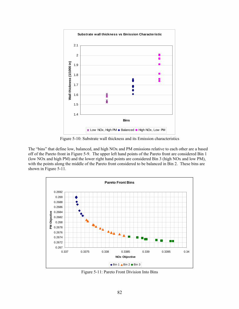
Substrate wall thickness vs Emission Characteristic
1.4
1.5
1.6
1.7
1.8
1.9
2
2.1
Bins
Wal
l thi
ckne
ss (1
/100
0 in
)
Low NOx, High PM Balanced High NOx, Low PM
Figure 5-10: Substrate wall thickness and its Emission characteristics The “bins” that define low, balanced, and high NOx and PM emissions relative to each other are a based off of the Pareto front in Figure 5-9. The upper left hand points of the Pareto front are considered Bin 1 (low NOx and high PM) and the lower right hand points are considered Bin 3 (high NOx and low PM), with the points along the middle of the Pareto front considered to be balanced in Bin 2. These bins are shown in Figure 5-11.
Pareto Front Bins
0.267
0.2672
0.2674
0.2676
0.2678
0.268
0.2682
0.2684
0.2686
0.2688
0.269
0.2692
0.337 0.3375 0.338 0.3385 0.339 0.3395 0.34
NOx Objective
PM O
bjec
tive
Bin 1 Bin 2 Bin 3
Figure 5-11: Pareto Front Division Into Bins
82
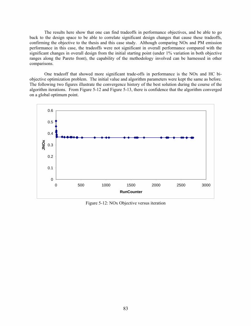
The results here show that one can find tradeoffs in performance objectives, and be able to go back to the design space to be able to correlate significant design changes that cause these tradeoffs, confirming the objective to the thesis and this case study. Although comparing NOx and PM emission performance in this case, the tradeoffs were not significant in overall performance compared with the significant changes in overall design from the initial starting point (under 1% variation in both objective ranges along the Pareto front), the capability of the methodology involved can be harnessed in other comparisons.
One tradeoff that showed more significant trade-offs in performance is the NOx and HC bi-objective optimization problem. The initial value and algorithm parameters were kept the same as before. The following two figures illustrate the convergence history of the best solution during the course of the algorithm iterations. From Figure 5-12 and Figure 5-13, there is confidence that the algorithm converged on a global optimum point.
0
0.1
0.2
0.3
0.4
0.5
0.6
0 500 1000 1500 2000 2500 3000
RunCounter
JNO
x
Figure 5-12: NOx Objective versus iteration
83

0
0.2
0.4
0.6
0.8
1
1.2
0 500 1000 1500 2000 2500 3000
RunCounter
JHC
Figure 5-13: Hydrocarbon Objective versus iteration
The following figures shows a set of the full 3000 design points, and Figure 5-15 shows the Pareto Optimal design points set, in objective space.
Design Points
0.55
0.6
0.65
0.7
0.75
0.8
0.33 0.335 0.34 0.345 0.35 0.355 0.36 0.365 0.37 0.375 0.38
NOx Objective (J NOx)
HC O
bjec
tive
(J H
C)
Design Points
Figure 5-14: Design Point Cloud (Found by GA)
84
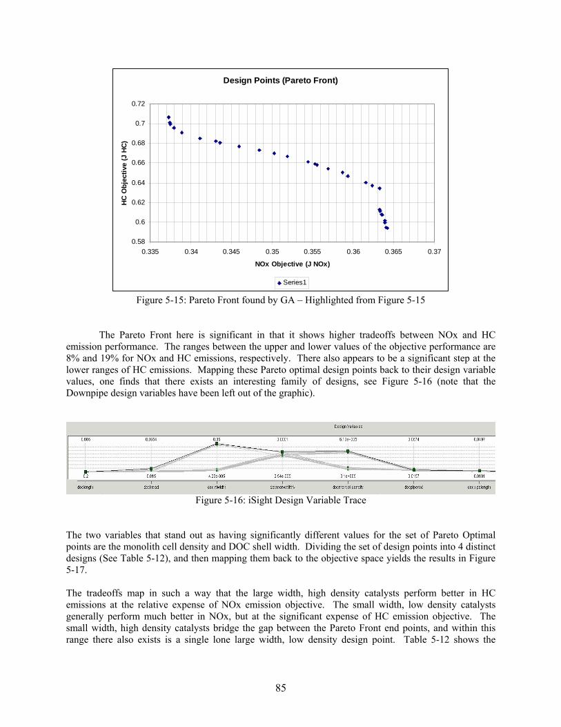
Design Points (Pareto Front)
0.58
0.6
0.62
0.64
0.66
0.68
0.7
0.72
0.335 0.34 0.345 0.35 0.355 0.36 0.365 0.37
NOx Objective (J NOx)
HC
Obj
ectiv
e (J
HC
)
Series1
Figure 5-15: Pareto Front found by GA – Highlighted from Figure 5-15
The Pareto Front here is significant in that it shows higher tradeoffs between NOx and HC emission performance. The ranges between the upper and lower values of the objective performance are 8% and 19% for NOx and HC emissions, respectively. There also appears to be a significant step at the lower ranges of HC emissions. Mapping these Pareto optimal design points back to their design variable values, one finds that there exists an interesting family of designs, see Figure 5-16 (note that the Downpipe design variables have been left out of the graphic).
Figure 5-16: iSight Design Variable Trace
The two variables that stand out as having significantly different values for the set of Pareto Optimal points are the monolith cell density and DOC shell width. Dividing the set of design points into 4 distinct designs (See Table 5-12), and then mapping them back to the objective space yields the results in Figure 5-17. The tradeoffs map in such a way that the large width, high density catalysts perform better in HC emissions at the relative expense of NOx emission objective. The small width, low density catalysts generally perform much better in NOx, but at the significant expense of HC emission objective. The small width, high density catalysts bridge the gap between the Pareto Front end points, and within this range there also exists is a single lone large width, low density design point. Table 5-12 shows the
85
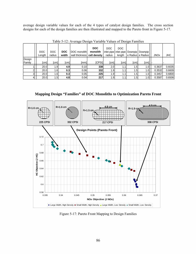
average design variable values for each of the 4 types of catalyst design families. The cross section designs for each of the design families are then illustrated and mapped to the Pareto front in Figure 5-17.
Table 5-12: Average Design Variable Values of Design Families
DOC Length
DOC radius
DOC width
DOC monolith wall thickness
DOC monolith
cell density
DOC inlet pipe
radius
DOC inlet pipe
lengthDownpipe Radius
Downpipe Radius JNOx JHC
Design Family [cm] [cm] [cm] [mm] [CPSI] [cm] [cm] [cm] [cm] - -
1 20.0 1.9 4.9 0.10 338 2.0 1.1 1.5 1.0 0.3637 0.60352 20.0 1.6 0.3 0.06 332 1.9 1.1 1.5 1.0 0.3532 0.66093 20.0 1.6 0.3 0.05 225 1.9 1.1 1.5 1.0 0.3457 0.68004 20.0 1.5 4.8 0.04 217 1.9 1.1 1.5 1.0 0.3587 0.6506
Mapping Design “Families” of DOC Monoliths to Optimization Pareto Front
Design Points (Pareto Front)
0.58
0.6
0.62
0.64
0.66
0.68
0.7
0.72
0.335 0.34 0.345 0.35 0.355 0.36 0.365 0.37
NOx Objective (J NOx)
HC O
bjec
tive
(J H
C)
Large Width, High Density Small Width, High Density Large Width, Low Density Small Width, Low Density
4.8 cmR=1.5 cm
217 CPSI
4.8 cmR=1.5 cm
217 CPSI
R=1.6 cm
225 CPSI
R=1.6 cm
225 CPSI
R=1.6 cm
332 CPSI
R=1.6 cm
332 CPSI
4.9 cmR=1.9 cm
338 CPSI
4.9 cmR=1.9 cm
338 CPSI
Figure 5-17: Pareto Front Mapping to Design Families
86
The behavior of these design variables shows that there can be multiple families of designs within the present architecture that optimize the catalyst for HC and NOx emissions, given the vehicle/engine combination and FTP cycle. These design families will most likely change for another given vehicle/engine and FTP cycle combination. The results of the DOC case study corroborate the potential existence of performance and cost trade-offs, as well as design families within a system architecture that directly impact the performance of the system.
5.10 Computational Effort
The modeling and simulation MATLAB/Simulink program would take approximately 2 to 8 seconds of computational time per evaluation. The performance varied depending on if there were graphics to plot or not, and also varied depending on the computer used. The faster computational times were completed on a Dell Optiplex GX620, with a Pentium D CPU 3.20 GHz, 3.5 GB of RAM. The slower computational time was on an IBM T42 Thinkpad, with a Pentium M 745 1.8 GHz, with 1 GB of RAM.
The first sets of optimization runs using the SQP gradient based algorithm took a total CPU time
of about 10 minutes to 50 minutes, depending on the starting point and number of iterations. The Genetic Algorithm and SQP combination, which required 1015 runs, took approximately 100 minutes to complete (the GA was initially seeded with the mid-range values, from which iSight then obtained the initial population). The initial design vector of midrange values was used as a seed. The bi-objective optimization results required 3030 total runs (30 initial population size, and 100 further generations), and took 3 hours and 58 minutes on the Dell Optiplex.
5.11 Conclusions of the DOC Case Study
Reviewing the initial objectives of the catalyst sizing case example, it can be concluded that the modeling capability of the tool developed to test the methodology presented has been validated. The modeling tool is capable of simulating a complete vehicle drive cycle and engine configuration through a given exhaust system model. Additionally, implementing design space exploration, trade studies, and optimization analysis has been achieved. The results and data from the simulation, as well as the optimization results, have been corroborated with understood behavior of the given components tested.
The proof of concept of a multi-disciplinary, system-wide analysis methodology applied to diesel exhaust systems shows promise in its ability to accurately model and analyze designs. The optimization implementation was also shown to give good analysis and can offer designers a better understanding of the system interactions. The detailed point to take away is that, just given the single catalyst type and vehicle/cycle combination, there are a number of design families that can optimize a multi-objective problem. The problem then can become more complex when combining other exhaust system components such as a diesel particulate filter and diesel oxidation catalyst.
Expanding the simulation model to include other components can potentially result in novel system designs that could not have been devised without a systems-wide methodology. This is explored in the next section that analyzes various system architectures in the methodology presented. Also, it was
87
found that the optimization loop can take into account the interplay between simulation components, in the programming architecture developed. This was important, in that it validated the approach towards the simulation and optimization codes and interfaces.
The significance of developing a modular system modeling methodology for diesel exhaust
systems design, analysis, and optimization is that it allows engineers to better analyze and understand the more complex after-treatment technologies that will be implemented in the future. The interactions among components are captured via the state-vector and potential feedback loops between components. The key point is that optimizing the exhaust system as a whole for a wide variety of operating points and engines during the pre-development design work is more valuable and beneficial than trying to adapt a single point design to be merely acceptable during the testing phase of product development. Being able to compare system components and architectures, as well as design parameters, gives engineers a better understanding of the performance and interactions of the system. Additionally, examining the entire system and its performance over a variety of conditions can lead to building a better overall system than combining single-point optimized components together, which is illustrated in Chapter 6 with a more complex case study. Engineers can take advantage of the interactions between components in the system and try to curb the downside effects. This is especially critical when after-treatment technologies are becoming more complex, potentially requiring active control in the future.
88
Chapter 6 . Multi-Objective and Multi-component Optimization: DOC/DPF Case Study
The significance of developing a modular system modeling methodology for diesel exhaust systems design, analysis, and optimization is that it allows engineers to better analyze and understand the more complex after-treatment technologies that will be implemented in the future. The interactions among components are captured via the state-vector (See Figure 3-2) and potential feedback loops between components. This is presented a new modular state-vector based modeling architecture and framework, as well as the software implementation of the modeling architecture. A proof of concept example was also presented, along with the results for a single objective optimization routine. Further design analysis into the initial results was also illustrated earlier.
The key point is that optimizing the exhaust system as a whole for a wide variety of operating points and engines during the pre-development design work is more valuable and beneficial than trying to adapt a single point design to be merely acceptable during the testing phase of product development or to assemble an exhaust treatment system as a collection of separately optimized components. Being able to compare system components and architectures, as well as design parameters, gives engineers a better understanding of the performance and interactions of the system. This knowledge can be used in the development process to refine designs in preparation for prototyping and testing. Additionally, examining the entire system and its performance over a variety of conditions can lead to building a better overall system than combining single-point optimized components together. Engineers can take advantage of the interactions between components in the system and try to curb the downside effects. This is especially critical when after-treatment technologies are becoming more complex, potentially requiring active control in the future.
Expanding the current simulation model to include other components (such as the Diesel Particulate Filter or Lean NOx Traps models) can potentially result in novel system designs that could not have been devised without a systems-wide methodology. Given the architecture and software implementation, engineers can expand the modeling and simulation tool further by adding other performance metrics, such as cost models. The methodology presented here supports system level design, analysis, and optimization of diesel after-treatment solutions, but could potentially be extended to other system design problems, particularly those involving various types of internal fluid flow.
89

6.1 Modeling Assumptions and Motivation
The optimization case study takes the modeling and simulation tool that was developed, and attempts to use a relevant example to illustrate the capabilities of the tool as well as investigate the optimization results of the comparative architecture systems. At the system level, the case study attempts to analyze three main objectives:
1. Investigate the performance of a completely passive system, specifically in its ability to
regenerate. 2. Investigate the performance of a dosing system and two heater systems, and compare that
with the passive system. 3. Attempt an optimization routine for the dosing and heater systems. Compare the final,
optimized, system architectures among each other.
By completing these three high level objectives, we can validate the capabilities not only of the modeling and simulation tool, but of the methodology objective of the thesis.
The dosing model, as shown in Figure 6-1, includes a system in front of the oxidation catalyst that injects diesel fuel spray over the catalyst. The increase in HC spray in the exhaust will cause a reaction in the oxidation catalyst that will raise the exhaust gas temperatures. This in turn, will be able to raise the temperature of both the DOC and DPF, and allow the DPF to regenerate.
The heater models are implemented pre-DOC and post-DOC, that is to say that the heater is located in front or behind the DOC. The implementation of the heater is a basic combustion system, that injects a fuel spray, utilizes a spark plug, and using the exhaust gas flow, will ignite the fuel spray and raise the exhaust gas temperature. The goal in comparing a pre- and post-DOC heater system is to examine the differences in performance, and to analyze the effects of HC slip of the combustor and how that affects emission performance.
The base case, passive system, and the three other system architectures are illustrated in Figure
6-1. The details of the modeling of the dosing model and heater/combustor model are in Appendix A.
The engine data used in the simulations is from a Cummins ISX 15.0 liter inline-6 cylinder engine. It was calibrated for model year 2004 emissions specifications, with a maximum speed of 2000 RPM, an idle speed of 600 RPM, and a maximum torque specification of 1247 lb-ft (or 1691 Nm). The DOC/DPF unit that was used as the baseline design is a production unit for Freightliner [5]. The operating conditions for the engine are a set of 20 steady state speed/load modes. These modes/points include the 13-modes in the European steady state cycle, as well as additional operating modes/points at lower engine speeds with moderate loadings. For the tests, the reference numbers 1 through 7 indicate the custom, low RPM, higher load conditions, and points 8 through 20 indicate the 13 different European steady state cycle points. Table 6-1 shows a table of the modes, comparing their load ratings (in percentage of maximum rated and absolute terms) and engine speed (in percentage of maximum rated and absolute terms)
90
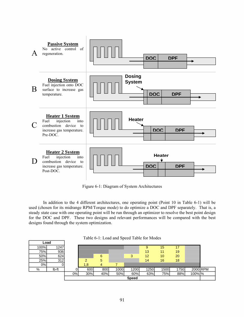
Passive System No active control of regeneration.
Figure 6-1: Diagram of System Architectures
In addition to the 4 different architectures, one operating point (Point 10 in Table 6-1) will be used (chosen for its midrange RPM/Torque mode) to do optimize a DOC and DPF separately. That is, a steady state case with one operating point will be run through an optimizer to resolve the best point design for the DOC and DPF. These two designs and relevant performances will be compared with the best designs found through the system optimization.
Table 6-1: Load and Speed Table for Modes
100% 1247 9 15 1775% 936 13 11 1950% 624 6 3 12 10 2025% 312 2 5 14 16 180% 0 1,8 4 7
% lb-ft 0 600 800 1000 1200 1250 1500 1750 2000 RPM0% 30% 40% 50% 60% 63% 75% 88% 100% %
Speed
Load
DOC DPF
DOC DPF
Dosing System
DOC DPF
Heater
DOC DPF
Heater
Dosing System Fuel injection onto DOC surface to increase gas temperature.
Heater 1 System Fuel injection into combustion device to increase gas temperature. Pre-DOC.
Heater 2 System Fuel injection into combustion device to increase gas temperature. Post-DOC.
A
B
C
D
91

6.2 Validation of Passive Regeneration
A diesel oxidation catalyst combined with a particulate filter, or a continuously regenerating trap, has a significant problem when it comes to the catalyst formulation versus regeneration behavior. The fundamental problem is that the particulate filter has to regenerate, also known as burning off the trapped particulate mass and soot to make room for more. The regeneration is needed to avoid increases in backpressure to unacceptable levels from the deposited particulate layer (see Chapter 4 for model details). The triggering of regeneration occurs when the exhaust temperature gasses allow it. However, those light-off temperatures are around 600° C. The exhaust gases rarely reach this level of temperature.
The first portion of this case study is to validate the phenomenon of the difficulty in being able to satisfactorily regenerate a particulate filter, passively, using simply the operating points of the engine. A set of the European steady state cycle operating points, as well as high load/near idle points, are used in the simulation program. These points are illustrated in Figure 6-2. Note that points 1 and 8 are the same (the order in the simulation is from a cold start at point 1, and then a return to idle at point 8 before going on). The simulation parameters used in these simulations are the same as in Chapter 5. The geometric variables are held constant, at the default values from the Freightliner DOC/DPF unit (see Appendix B for calibration results) are shown in Table 6-2.
Table 6-2: Baseline Design Variables
Variable Default Value
Exhaust Down Pipe Radius 6 cm Exhaust Down Pipe Length (overall) 1.5 m DOC Overall length 13.6 cm DOC Radius 15.5 cm DOC Monolith Wall Thickness 5 mil (0.13 mm) DOC Monolith Cell Density 300 cpsi DPF Overall length 38.1 cm DPF Radius 16.5 cm DPF Monolith Wall Thickness 12 mil (0.305 mm) DPF Monolith Cell Density 200 cpsi
Engine Operation Map
1 4
5
6
7
9
10
11
12
13
14
15
16
17
18
19
20
2
3
80.0%
20.0%
40.0%
60.0%
80.0%
100.0%
120.0%
0.0% 20.0% 40.0% 60.0% 80.0% 100.0%
Speed (percentage of max RPM)
Torq
ue (p
erce
ntag
e of
max
Tor
que)
Figure 6-2: Engine Operating Map
92

The results of the simulations show that the lower load operating points do not operate in a
regime that allows for particulate filter regeneration. The typical temperature and collected mass graphics of the simulations at these points are represented in Figure 6-3, Figure 6-4, and Figure 6-5.
Figure 6-3: Collected Mass in DPF (total and for each layer/slab in wall) - Point 12
Figure 6-4: DOC Temperature Trace – Point 12
Note that the DOC and DPF temperatures do not reach the critical 600 °C needed for
regeneration.
93

Figure 6-5: DPF Temperature Trace – Point 12
As can be seen, the temperature of the exhaust gas in and out of the unit does not rise to a level
that will typically allow for filter regeneration. The simulation also shows this in the particulate mass loading graphic in Figure 6-3. Each section of the simulated slab, as well as the soot layer, and the total particulate mass loading is represented in the graphic. A typical regeneration graphic for particulate mass loading will show an increase in total mass to a peak, and then a decrease to a steady state level that signifies a burning off of the particulate mass. However, any graphic that shows a steadily increasing total particulate mass collection identifies no regeneration. For the majority of operating points, the temperature never reaches the level required for light-off of regeneration. The exhaust gas temperatures generally range between 100°C and 450°C, and once the system reaches a steady state level of operation.
However, the only points that successfully regenerate, at some rate, are operating points 9, 15, and 17, which are points are at the maximum load condition (maximum torque output). It is evident from the plots that as the temperature increase to above 600°C, and becomes steady, the particulate mass in the filter at first increases (as it collects/traps it), and then once the light-off temperature is reached, the particulate matter is oxidized and burned off at a faster rate than what is collected. However, the system then reaches an equilibrium of particulate mass within the filter. This illustrates that the trap is collecting mass at the same rate that it is converting it (burning it off). In addition, note that there is minimal temperature drop through the DOC, and in some cases there is a temperature rise (as the exothermic reactions in the DOC take effect). In summary, we only have successful regeneration when the engine can operate at higher RPM and at maximum loading state. Note that points 9, 15, and 17 correspond to Euro 2, 8, and 10, respectively.
94
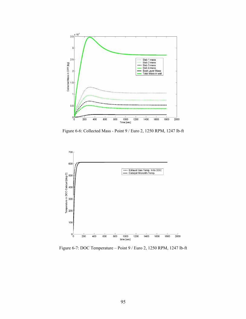
Figure 6-6: Collected Mass - Point 9 / Euro 2, 1250 RPM, 1247 lb-ft
Figure 6-7: DOC Temperature – Point 9 / Euro 2, 1250 RPM, 1247 lb-ft
95
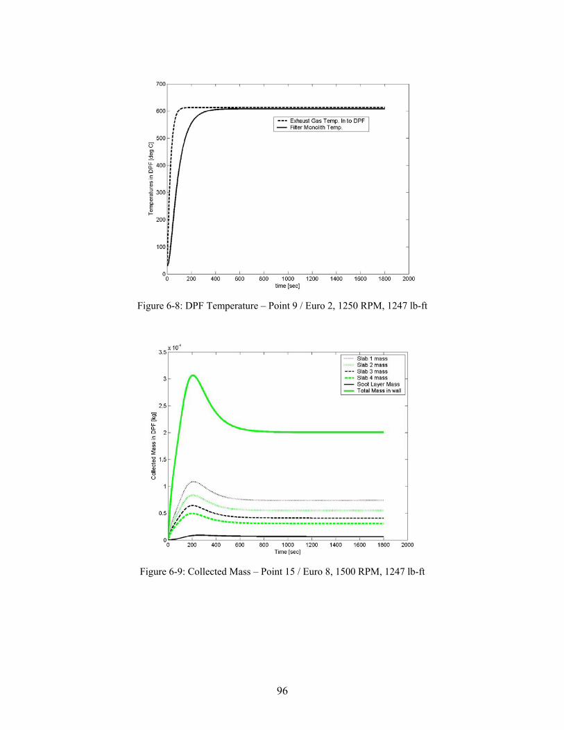
Figure 6-8: DPF Temperature – Point 9 / Euro 2, 1250 RPM, 1247 lb-ft
Figure 6-9: Collected Mass – Point 15 / Euro 8, 1500 RPM, 1247 lb-ft
96

Figure 6-10: DOC Temperature – Point 15 / Euro 8, 1500 RPM, 1247 lb-ft
Figure 6-11: DPF Temperature – Point 15 / Euro 8, 1500 RPM, 1247 lb-ft
97

Figure 6-12: Collected Mass – Point 17 / Euro 10, 1750 RPM, 1247 lb-ft
Figure 6-13: DOC Temperatures – Point 17 / Euro 10, 1750 RPM, 1247 lb-ft
98
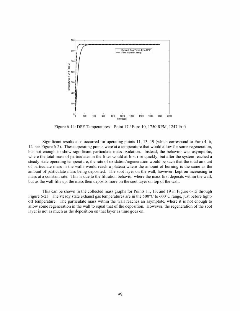
Figure 6-14: DPF Temperatures – Point 17 / Euro 10, 1750 RPM, 1247 lb-ft
Significant results also occurred for operating points 11, 13, 19 (which correspond to Euro 4, 6, 12, see Figure 6-2). These operating points were at a temperature that would allow for some regeneration, but not enough to show significant particulate mass oxidation. Instead, the behavior was asymptotic, where the total mass of particulates in the filter would at first rise quickly, but after the system reached a steady state operating temperature, the rate of oxidation/regeneration would be such that the total amount of particulate mass in the walls would reach a plateau where the amount of burning is the same as the amount of particulate mass being deposited. The soot layer on the wall, however, kept on increasing in mass at a constant rate. This is due to the filtration behavior where the mass first deposits within the wall, but as the wall fills up, the mass then deposits more on the soot layer on top of the wall.
This can be shown in the collected mass graphs for Points 11, 13, and 19 in Figure 6-15 through
Figure 6-23. The steady state exhaust gas temperatures are in the 500°C to 600°C range, just before light-off temperature. The particulate mass within the wall reaches an asymptote, where it is hot enough to allow some regeneration in the wall to equal that of the deposition. However, the regeneration of the soot layer is not as much as the deposition on that layer as time goes on.
99

Figure 6-15: Collected Mass – Point 11 / Euro 4, 1500 RPM, 936 lb-ft
Figure 6-16: DOC Temperatures – Point 11 / Euro 4, 1500 RPM, 936 lb-ft
100

Figure 6-17: DPF Temperatures – Point 11 / Euro 4, 1500 RPM, 936 lb-ft
Figure 6-18: Collected Mass – Point 13 / Euro 6, 1250 RPM, 936 lb-ft
101

Figure 6-19: DOC Temperatures – Point 13 / Euro 6, 1250 RPM, 936 lb-ft
Figure 6-20: DPF Temperatures – Point 13 / Euro 6, 1250 RPM, 936 lb-ft
102

Figure 6-21: Collected Mass – Point 19 / Euro 12, 1750 RPM, 936 lb-ft
Figure 6-22: DOC Temperatures – Point 19 / Euro 12, 1750 RPM, 936 lb-ft
103
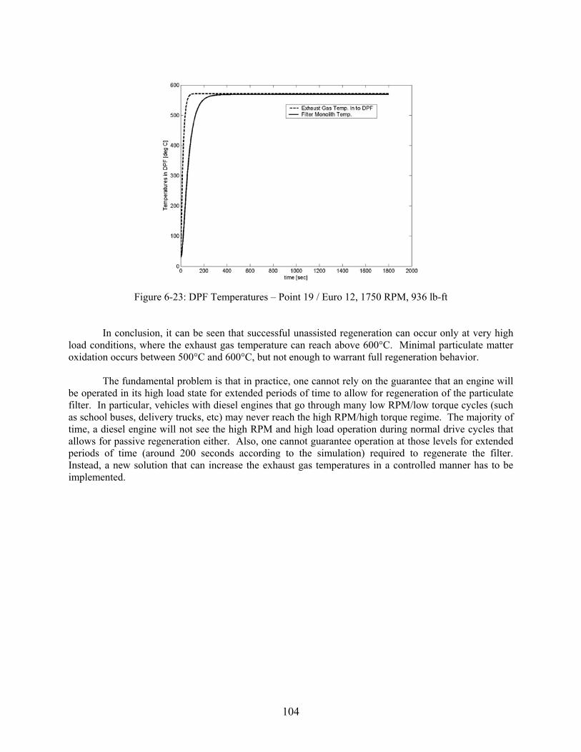
Figure 6-23: DPF Temperatures – Point 19 / Euro 12, 1750 RPM, 936 lb-ft
In conclusion, it can be seen that successful unassisted regeneration can occur only at very high load conditions, where the exhaust gas temperature can reach above 600°C. Minimal particulate matter oxidation occurs between 500°C and 600°C, but not enough to warrant full regeneration behavior.
The fundamental problem is that in practice, one cannot rely on the guarantee that an engine will be operated in its high load state for extended periods of time to allow for regeneration of the particulate filter. In particular, vehicles with diesel engines that go through many low RPM/low torque cycles (such as school buses, delivery trucks, etc) may never reach the high RPM/high torque regime. The majority of time, a diesel engine will not see the high RPM and high load operation during normal drive cycles that allows for passive regeneration either. Also, one cannot guarantee operation at those levels for extended periods of time (around 200 seconds according to the simulation) required to regenerate the filter. Instead, a new solution that can increase the exhaust gas temperatures in a controlled manner has to be implemented.
104

Regeneration Mapping to Engine Operating Point
0.0%
20.0%
40.0%
60.0%
80.0%
100.0%
120.0%
0.0% 20.0% 40.0% 60.0% 80.0% 100.0%
Speed (percentage of max RPM)
Torq
ue (p
erce
ntag
e of
max
Tor
que)
Full Regeneration Partial Regeneration No Regeneration
Figure 6-24: Regeneration Map of Engine Operating Points
Figure 6-24 shows the regeneration state mapping to the engine operating points. The highlighted points indicate engine operating points that allow for regeneration, and states of partial regeneration. The remaining points indicate no regeneration, or purely trapping conditions.
The comparison that will be shown for the purposes of the case study will be 3 different
architectures. The first is a dosing component, and the second and third will be a heater component that puts the combustion device in front of the DOC and then between the DOC and DPF. The dosing and heating models are described in Chapter 4 and Appendix A with greater detail.
6.3 Design Variables and Constraints
The design variables for the three different system architectures should incorporate the different catalyst formulations and geometric variables that can primarily affect the emission conversion efficiency performance, the particulate mass conversion, and that reflect the costs associated with producing these systems. Additionally, the dosing system and the combustion/heater system include the fuel injection parameters that will affect the fuel economy penalty during daily operation.
Table 6-3: Exhaust Downpipe Dimensioning Parameters Variable Default/Initial
Value Lower
Boundary Upper
Boundary
Pipe Radius 6 cm 3 cm 9 cm Pipe Length (overall) 1.5 m 0.5 m 3 m
105

Table 6-4: Diesel Oxidation Catalyst Dimensioning Variables
Variable Default/Initial Value
Lower Boundary
Upper Boundary
Overall length 13.6 cm 5 cm 50 cm Radius 15.5 cm 5 cm 25 cm Monolith Wall Thickness
5 mil (0.13 mm)
1 mil (0.03 mm)
7 mil (0.18 mm)
Monolith Cell Density 300 cpsi 200 cpsi 400 cpsi
Table 6-5: Diesel Particulate Filter Dimensioning Variables Variable Default/Initial
Value Lower
Boundary Upper
Boundary
Overall length 38.1 cm 5 cm 50 cm Radius 16.5 cm 5 cm 25 cm Monolith Wall Thickness
12 mil (0.305 mm)
8 mil (0.21 mm)
17 mil (0.432 mm)
Monolith Cell Density 200 cpsi 100 cpsi 300 cpsi
Table 6-6: Heater/Combustor System Design Variables Variable Default/Initial
Value Lower
Boundary Upper
Boundary
Heater Interval 1400 seconds 1400 seconds 1400 seconds Length of Heating Time (as percent of interval)
6% (84 sec) 6% (84 sec) 6% (84 sec)
Fuel Flow 2 g/s 0.5 g/s 4 g/s
Table 6-7: Dosing System Design Variables Variable Default/Initial
Value Lower
Boundary Upper
Boundary
Dosing Interval 1400 seconds 1400 seconds 1400 seconds Dosing Rate Multiplier 1.5 0.5 2.5 Length of Dosing (as percent of interval)
6% (84 sec) 6% (84 sec) 6% (84 sec)
As described in Section 6.1, the dosing system is a system in which diesel fuel is sprayed over the
DOC in order to allow for the catalytic reaction that occurs on the DOC to raise the temperature of the exhaust gas to allow the DPF to regenerate. The dosing interval is a set time at which the dosing occurs during the operating point. Overall, the steady state simulation captures 1800 seconds for each operating point, and the dosing occurs at the 1400 second time stamp, and the length of the dosing is set at 84 seconds. The dosing rate multiplier variable is a multiplier for the dosing curve - a parameter that matches the exhaust gas temperature to the comparative amount of hydrocarbon spray required at that temperature to be able to raise the exhaust gas temperature to levels required for regeneration. The multiplier variable is a sizing parameter that allows the dosing curve to vary depending on the size of the DOC. The default curve is shown in Figure 6-25.
106
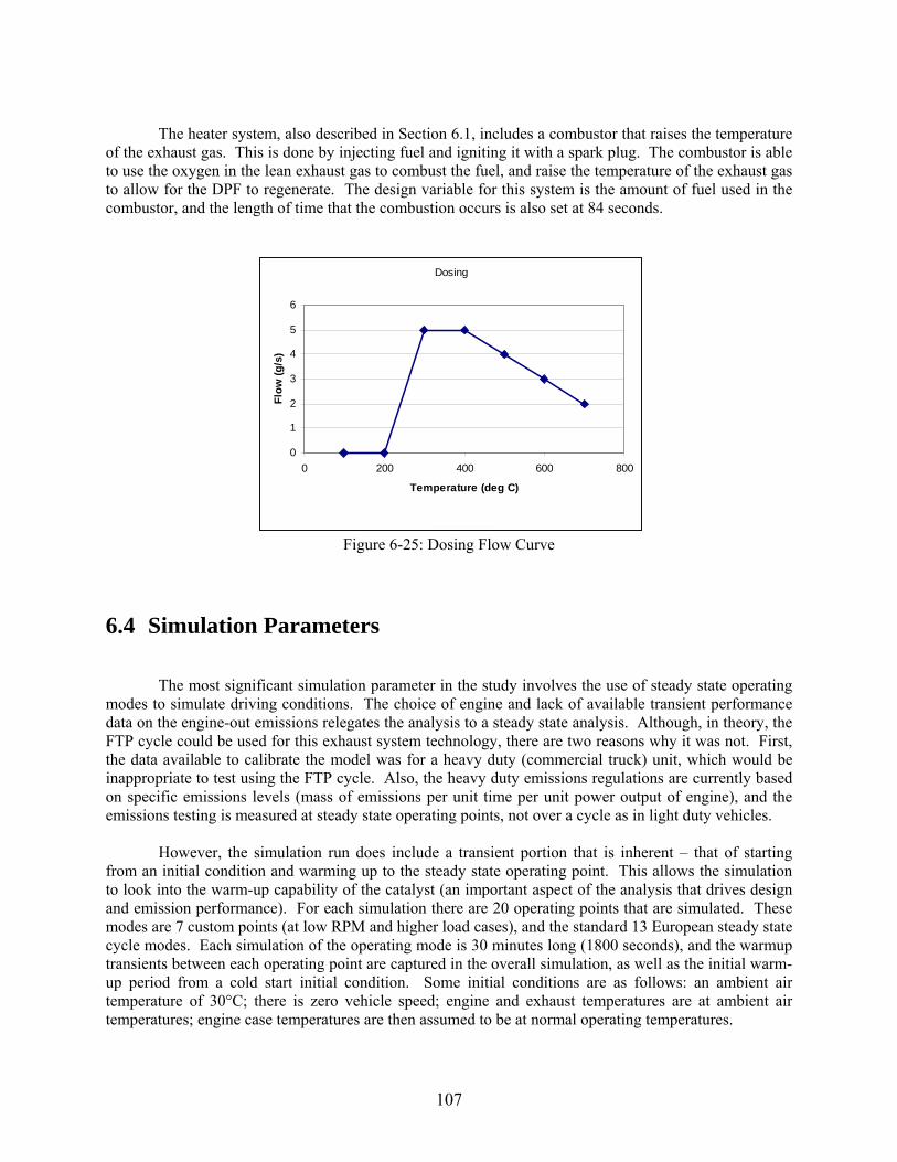
The heater system, also described in Section 6.1, includes a combustor that raises the temperature
of the exhaust gas. This is done by injecting fuel and igniting it with a spark plug. The combustor is able to use the oxygen in the lean exhaust gas to combust the fuel, and raise the temperature of the exhaust gas to allow for the DPF to regenerate. The design variable for this system is the amount of fuel used in the combustor, and the length of time that the combustion occurs is also set at 84 seconds.
Dosing
0
1
2
3
4
5
6
0 200 400 600 800
Temperature (deg C)
Flow
(g/s
)
Dosing
Figure 6-25: Dosing Flow Curve
6.4 Simulation Parameters
The most significant simulation parameter in the study involves the use of steady state operating
modes to simulate driving conditions. The choice of engine and lack of available transient performance data on the engine-out emissions relegates the analysis to a steady state analysis. Although, in theory, the FTP cycle could be used for this exhaust system technology, there are two reasons why it was not. First, the data available to calibrate the model was for a heavy duty (commercial truck) unit, which would be inappropriate to test using the FTP cycle. Also, the heavy duty emissions regulations are currently based on specific emissions levels (mass of emissions per unit time per unit power output of engine), and the emissions testing is measured at steady state operating points, not over a cycle as in light duty vehicles.
However, the simulation run does include a transient portion that is inherent – that of starting
from an initial condition and warming up to the steady state operating point. This allows the simulation to look into the warm-up capability of the catalyst (an important aspect of the analysis that drives design and emission performance). For each simulation there are 20 operating points that are simulated. These modes are 7 custom points (at low RPM and higher load cases), and the standard 13 European steady state cycle modes. Each simulation of the operating mode is 30 minutes long (1800 seconds), and the warmup transients between each operating point are captured in the overall simulation, as well as the initial warm-up period from a cold start initial condition. Some initial conditions are as follows: an ambient air temperature of 30°C; there is zero vehicle speed; engine and exhaust temperatures are at ambient air temperatures; engine case temperatures are then assumed to be at normal operating temperatures.
107

It is important to note that both the heater and dosing systems are triggered only when the exhaust gas temperature reaches a set value. This is done in order to prevent regeneration attempts at idle and low RPM/low torque conditions, when it is very near impossible for any system to be able to sufficiently raise the temperature of the exhaust gas enough to allow for regeneration of the DPF.
6.5 Objectives
In order to compare the system architectures and the designs between them, a set of objectives was developed. The goal of the objective sets is to resolve the emission performance, regeneration capabilities and cost objectives. In order to compare the different sets of objectives it is necessary to normalize the objective function values. By having normalized objectives, a multi-objective algorithm can more easily handle the differences inherent in measuring different performance qualities using different units. Normalizing the objective functions brings the gradient vector within the same order of magnitude, and thus can better correlate changes in the objective space with the relative changes in the design variables. There will thus be fewer problems associated with artificially increased sensitivity from poorly comparing objectives with widely differing magnitudes. Also, the end goal of most designers using a system such as this is to be able to have some form of comparative analysis between an initial design or requirements versus the optimal solution sets. Note also that the objectives are averaged over all of the operating modes for each case, with equal weight given by definition to each operating mode.
6.5.1 Performance Objectives:
In general, CO and HC emission levels for diesel engines are comparatively easy to meet compared to Particulates and NOx emissions. The critical emissions problem in recent years has been the ability for the engines to meet the particulate and NOx regulations. However, as a system, it is necessary to investigate the overall balance, effect, and interactions between the different emissions species. From the four main emission species, two overall emission objectives are defined, the average overall conversion efficiency and the average overall conversion efficiency for particulates and NOx. Performance Objective Set 1: Maximize Emission Conversion Efficiencies
• PM_eff = 1 – (PM_out/PM_in) • NOx_eff = 1 – (NOx_out/NOx_in) • HC_eff = 1 – (HC_out/HC_in) • CO_eff = 1 – (CO_out/CO_in)
Performance Objective Set 2: Maximize Average System Efficiencies
• Avg_eff = ¼(PM_eff + NOx_eff + HC_eff + CO_eff) • NOx_PM_eff = ½(PM_eff+NOx_eff)
For the purposes of this optimization, Objective Set 2 will be used as a performance objective for emission conversion efficiency. Unlike the first case study in Chapter 5, the regulatory limits are not used in this case to normalize the emissions objectives for two reasons. First, there are some operating points in the simulation that are not included in the emissions testing, but are included in the simulation and objective criteria in order to gain a better understanding of the regeneration behavior at lower loads and RPMs. Also, the engine and production DOC/DPF unit that the model is based off of already meets current emissions regulations; and this case requires purely a comparative analysis between various
108
designs and architectures - passing emissions standards is not an absolute criteria in the performance objective.
6.5.2 Regeneration Objectives:
Investigating the regeneration behavior of the DPF is important for measuring the performance capability of the DPF in terms of its ability to control PM emissions while regenerating, identifying and longevity or reliability issues (thermal cycling), and assessing the fuel economy impact. The fuel economy impact can be quite significant if one is using a combustion process to heat the exhaust gas for regeneration, or if using a dosing system to spray hydrocarbon over the DOC to increase exhaust gas temperatures.
The objectives, then, are to measure the effectiveness of the regeneration process and its fuel economy impact. For each steady state condition, a set fuel dosing strategy is implemented to consistently raise the temperatures to the levels required for regeneration. A similar strategy is used in the exhaust heater system. Each regeneration is then set to operate over a set time period near the end point of the simulation where the state of the system is near equilibrium. Then, the total fuel penalty is measured from the simulation, along with the percentage of particulate mass oxidized from the DPF. Regeneration Objective Set: Minimize fuel economy penalty
• Fuel Economy Penalty = Mass fuel used for regeneration • Normalized Fuel Econ. Penalty = Mass fuel used /( 10%*total fuel used in operation)
Regeneration Objective Set: Maximize PM conversion efficiency
• Regeneration Capability = Successful regenerations / No. of Regen. attempts • Regeneration Efficiency = Mass PM burned / Mass PM at start of burn
The normalized fuel economy penalty calculation was done using an a priori set 10% limit of fuel consumption. The value for 10% was derived from the maximum fuel economy penalty that heavy duty commercial operators have been generally known to willingly accept. The regeneration efficiency is also calculated as the mass of particulates burned over the mass of particulates in the DPF at the start of the burn, for each operating point that regeneration is attempted for. This regeneration efficiency of each operating point for which it is attempted is then averaged.
6.5.3 Cost Objectives:
Fundamentally, the cost of a DOC/DPF system is dependent on the size of the monolith substrate used and the overall mass of the system. The raw material costs tend to drive the cost of the system, as the manufacturing costs consist purely of metal fabrication and its assembly more so than the assembly process and its labor. In order to achieve any significant cost savings, the system has to use less material. In addition, the amount and type of material used to manufacture the monolith substrates is also a function of cost. The platinum loading parameter of catalysts is generally used to gauge its cost, since more dense platinum metal loading generally costs more. Filter and catalyst manufacturers also increase costs as monolith wall thickness decreases and as cell density increases. These costs are proprietary information, and therefore the cost objectives will be simplified to be purely a function of mass of the system and the monolith substrate masses.
109

Cost Objective Set: Minimize Mass • Mass of DOC monolith substrate • Mass of DPF monolith substrate • Mass of system • Normalized Mass of DOC = Mass of DOC / (150%*Default Mass of DOC) • Normalized Mass of DPF = Mass of DPF / (150%*Default Mass of DPF) • Normalized Mass of system = Mass of system / (150%*Default Mass of system)
The normalized mass of the system is calculated from 150% of the mass of the default DOC/DPF system. This default mass value is calculated from the current production DOC/DPF unit; and the 150% value stems from the generally accepted increase in cost that a manufacturer is willing to incur for better performance.
6.5.4 Objectives Used During Optimization Routine
In order to simply the case study, and to avoid having the simulation and optimization run times become inordinately long, four objectives were chosen a priori to the optimization. These objectives represent the main goals behind the system from various disciplines, and summarized in Table 6-8.
Table 6-8: Objective Table • Minimize: Normalized Mass of System Represents the associated manufacturing costs • Maximize: NOx and PM Efficiency Represents the critical emission performance of the
DOC/DPF unit • Minimize: Fuel Economy Penalty Represents operating costs associated with fuel • Maximize: Regeneration Efficiency Represents the regeneration performance of the
doser or heating system
6.6 Initial Design Points and Architecture Comparison The following section includes the results of the initial design point simulations and performance comparison of the designs of each architecture. The sections include the appropriate design tables and Performance Tables for the 8 objectives.
6.6.1 Initial Passive System See Figure 6-1, Part A for a visual representation of the passive system.
110

Table 6-9: Passive System Design Table Variable Value
Exhaust Down Pipe Radius 6 cm Exhaust Down Pipe Length (overall) 1.5 m DOC Overall length 13.6 cm DOC Radius 15.5 cm DOC Monolith Wall Thickness 5 mil (0.13 mm) DOC Monolith Cell Density 300 cpsi DPF Overall length 38.1 cm DPF Radius 16.5 cm DPF Monolith Wall Thickness 12 mil (0.305 mm) DPF Monolith Cell Density 200 cpsi
Table 6-10: Passive System Performance Table Mode \ Objective Avg_eff
(max) NOx & PM Eff (max)
Fuel Econ. Penalty (min)
Regen capable (max)
Regen Eff (max)
DOC Mass
DPF Mass
System Mass
Custom 1 / Point 1 0.2264 0.4528 0 0 0 0.6666 0.6671 0.6666 Custom 2 / Point 2 0.3357 0.5362 0 0 0 0.6666 0.6671 0.6666 Custom 3 / Point 3 0.2261 0.4133 0 0 0 0.6666 0.6671 0.6666 Custom 4 / Point 4 0.2414 0.4761 0 0 0 0.6666 0.6671 0.6666 Custom 5 / Point 5 0.6026 0.7150 0 0 0 0.6666 0.6671 0.6666 Custom 6 / Point 6 0.7484 0.8184 0 0 0 0.6666 0.6671 0.6666 Custom 7 / Point 7 0.2201 0.4242 0 0 0 0.6666 0.6671 0.6666 Euro 1 / Point 8 0.2264 0.4528 0 0 0 0.6666 0.6671 0.6666 Euro 2 / Point 9 0.7349 0.7940 0 1 0.1906 0.6666 0.6671 0.6666 Euro 3 / Point 10 0.6837 0.7550 0 0 0 0.6666 0.6671 0.6666 Euro 4 / Point 11 0.7237 0.7836 0 0 0 0.6666 0.6671 0.6666 Euro 5 / Point 12 0.7264 0.7960 0 0 0 0.6666 0.6671 0.6666 Euro 6 / Point 12 0.7362 0.7983 0 0 0 0.6666 0.6671 0.6666 Euro 7 / Point 12 0.5699 0.6750 0 0 0 0.6666 0.6671 0.6666 Euro 8 / Point 12 0.7164 0.7740 0 1 0.1550 0.6666 0.6671 0.6666 Euro 9 / Point 12 0.5603 0.6587 0 0 0 0.6666 0.6671 0.6666 Euro 10 / Point 12 0.7118 0.7657 0 1 0.0444 0.6666 0.6671 0.6666 Euro 11 / Point 12 0.5710 0.6616 0 0 0 0.6666 0.6671 0.6666 Euro 12 / Point 12 0.7142 0.7705 0 0 0 0.6666 0.6671 0.6666 Euro 13 / Point 12 0.6950 0.7600 0 0 0 0.6666 0.6671 0.6666
Average of each point, independently
0.5485 0.6640 0 0.1500 0.1300 0.6666 0.6671 0.6666
Overall Simulation Average
0.613 0.742 0 0.150 0.130* 0.666 0.667 0.666
* Efficiency of Regenerations Attempted, Not of All Operation Points Each operating point was initially simulated to order to better gauge a comparison between them in the overall behavior of the passive system. Again, this shows that there are only 3 points that are capable to regenerate, and out of these the best efficiency of for the regeneration is just about 20%. The average regeneration efficiency is just 13% overall. The operating points were then combined together as per the simulation parameters, and the emission conversion efficiencies then calculated. These efficiencies are higher than the average for each point done independently because of the fact that the
111
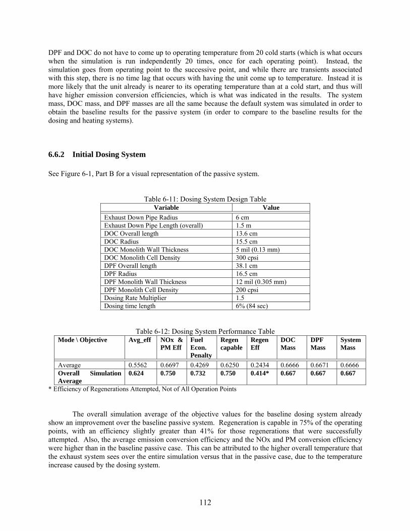
DPF and DOC do not have to come up to operating temperature from 20 cold starts (which is what occurs when the simulation is run independently 20 times, once for each operating point). Instead, the simulation goes from operating point to the successive point, and while there are transients associated with this step, there is no time lag that occurs with having the unit come up to temperature. Instead it is more likely that the unit already is nearer to its operating temperature than at a cold start, and thus will have higher emission conversion efficiencies, which is what was indicated in the results. The system mass, DOC mass, and DPF masses are all the same because the default system was simulated in order to obtain the baseline results for the passive system (in order to compare to the baseline results for the dosing and heating systems).
6.6.2 Initial Dosing System See Figure 6-1, Part B for a visual representation of the passive system.
Table 6-11: Dosing System Design Table Variable Value
Exhaust Down Pipe Radius 6 cm Exhaust Down Pipe Length (overall) 1.5 m DOC Overall length 13.6 cm DOC Radius 15.5 cm DOC Monolith Wall Thickness 5 mil (0.13 mm) DOC Monolith Cell Density 300 cpsi DPF Overall length 38.1 cm DPF Radius 16.5 cm DPF Monolith Wall Thickness 12 mil (0.305 mm) DPF Monolith Cell Density 200 cpsi Dosing Rate Multiplier 1.5 Dosing time length 6% (84 sec)
Table 6-12: Dosing System Performance Table Mode \ Objective Avg_eff NOx &
PM Eff Fuel Econ. Penalty
Regen capable
Regen Eff
DOC Mass
DPF Mass
System Mass
Average 0.5562 0.6697 0.4269 0.6250 0.2434 0.6666 0.6671 0.6666 Overall Simulation Average
0.624 0.750 0.732 0.750 0.414* 0.667 0.667 0.667
* Efficiency of Regenerations Attempted, Not of All Operation Points The overall simulation average of the objective values for the baseline dosing system already show an improvement over the baseline passive system. Regeneration is capable in 75% of the operating points, with an efficiency slightly greater than 41% for those regenerations that were successfully attempted. Also, the average emission conversion efficiency and the NOx and PM conversion efficiency were higher than in the baseline passive case. This can be attributed to the higher overall temperature that the exhaust system sees over the entire simulation versus that in the passive case, due to the temperature increase caused by the dosing system.
112

It is important to also note that when taken independently, from cold starts, regeneration was capable in only 63% of operating points, as opposed to the overall simulation average of 75%. This can be attributed to the “borderline” cases at lower RPM and torque regimes. There can be cases at the borderline, where the exhaust has not fully come up to temperature from a cold start, and thus the temperature of the gas did not trigger the dosing system to operate. However, during the overall simulation, since the exhaust has come up to temperature during the first few operating points, the system may have enough latent heat to trigger the regeneration. The higher latent heat is also a reason why the regeneration efficiency is slightly higher.
6.6.3 Initial Heater System 1 See Figure 6-1, Part C for a visual representation of the passive system.
Table 6-13: Heater System 1 Design Table Variable Value
Exhaust Down Pipe Radius 6 cm Exhaust Down Pipe Length (overall) 1.5 m DOC Overall length 13.6 cm DOC Radius 15.5 cm DOC Monolith Wall Thickness 5 mil (0.13 mm) DOC Monolith Cell Density 300 cpsi DPF Overall length 38.1 cm DPF Radius 16.5 cm DPF Monolith Wall Thickness 12 mil (0.305 mm) DPF Monolith Cell Density 200 cpsi Length of Time of Heating (as percent of interval) 6% (84 sec) Fuel Flow 2 g/s
Table 6-14: Heater System 1 Performance Table Mode \ Objective Avg_eff NOx &
PM Eff Fuel Econ. Penalty
Regen capable
Regen Eff
DOC Mass
DPF Mass
System Mass
Average 0.5350 0.6706 0.1336 0.7143 0.4144 0.6666 0.6671 0.6666 Overall Simulation Average
0.596 0.750 0.172 0.786 0.486* 0.667 0.667 0.667
* Efficiency of Regenerations Attempted, Not of All Operation Points The overall simulation average of some of the objective values for the baseline heater 1 system shows an improvement over the baseline passive system. Regeneration is capable in 79% of the operating points, with an efficiency slightly greater than 49% for those regenerations that were successfully attempted, this is higher than the dosing system, and the fuel economy penalty is also less than that of the dosing system. Also, the average emission conversion efficiency and the NOx and PM conversion efficiency were higher than in the baseline passive case, but not as good as the baseline dosing system case. This difference could be attributed to fact that the DOC may not be responding as well in the dosing case, because there much less addition of hydrocarbons to the exhaust flow in the heater system, whereas in the dosing system there is a fuel sprayed directly over the DOC. Also, the heater system has a certain
113

amount of hydrocarbon slip due to inefficiencies in the combustion process. This slip value is assumed to be at around 5%, and this can be causing the lower average emission conversion value.
6.6.4 Initial Heater System 2 See Figure 6-1, Part D for a visual representation of the passive system.
Table 6-15: Heater System 2 Design Table Variable Value
Exhaust Down Pipe Radius 6 cm Exhaust Down Pipe Length (overall) 1.5 m DOC Overall length 13.6 cm DOC Radius 15.5 cm DOC Monolith Wall Thickness 5 mil (0.13 mm) DOC Monolith Cell Density 300 cpsi DPF Overall length 38.1 cm DPF Radius 16.5 cm DPF Monolith Wall Thickness 12 mil (0.305 mm) DPF Monolith Cell Density 200 cpsi Length of Time of Heating (as percent of interval) 6% (84 sec) Fuel Flow 2 g/s
Table 6-16: Heater System 2 Performance Table Mode \ Objective Avg_eff NOx &
PM Eff Fuel Econ. Penalty
Regen capable
Regen Eff
DOC Mass
DPF Mass
System Mass
Average 0.4313 0.6632 0.1336 0.6429 0.4084 0.6666 0.6671 0.6666 Overall Simulation Average
0.456 0.741 0.171 0.714 0.465* 0.667 0.667 0.667
* Efficiency of Regenerations Attempted, Not of All Operation Points The overall simulation average of the objective values for the baseline Heater 2 system are somewhat different than the Heater 1 System. Overall, it appears to be a less efficient system, both in terms of regeneration capability and efficiency, and in terms of emission conversion performance. However, it should be noted, that the Heater 2 System, similar to the Heater 1 System but in an even worse situation, has a problem in the hydrocarbon slip past the combustor. This is also an issue in that the Heater 2 System doesn’t allow that hydrocarbon to be reacted in the DOC. Already in these test cases, we see the interplay that can occur from seemingly disparate systems. For example, the Heater 2 System doesn’t allow the hydrocarbon slip that occurs in the combustor to have a chance to be reacted by the DOC, whereas the Heater 1 System does. Also, we find that the amount of hydrocarbon spray that is added to the exhaust system affects the performance and thus heat generated within the DOC. The heater and dosing system’s goal of raising the temperature for DPF regeneration is occurring, but at costs to the emission performance. Also, there are significant costs associated with the fuel penalty between the dosing and heating systems. A great deal more fuel is needed to be vaporized and sprayed over the DOC to raise the temperature than to burn it in the heating systems, and thus the dosing system has a fuel penalty nearly 5 times higher than the heating systems.
114

6.7 Coarse Objective Space Results and Architectural Comparisons In order to obtain a valid comparative study between the architectures, a Genetic Algorithm [6, 13, 34] was set-up to perform a trade-off analysis between competing objectives and yield an objective space optimization. The GA was used in order to obtain a coarse objective space exploration, which then should yield some design directions that could be further refined. Performing the GA for each case yielded a best design (as chosen by the iSight algorithm) in the Table 6-17. The NSGA-II Algorithm used in iSight treated each objective is separately, and used non-dominated sorting and crowding distance sorting as the two main mechanisms in the selection process. The population size was set to 40 individual designs, with an initial set of 10 generations. The small number of generations was used due to the limited computational capability of the computer to run through a larger set of iterations. As such, each case took 440 iterations and roughly 20 hours to compute. Each case’s iteration is 1 loop through all 20 operating conditions, as explained in section 6.6. The objectives for the case studies were set as the following (also shown in Table 6-8):
• Maximize: NOx and PM Conversion Efficiency • Minimize: Fuel Penalty • Maximize: Regeneration Efficiency • Minimize: System Mass
Table 6-17: Best Solutions Found For Each Architecture using NSGA-II Genetic Algorithm in iSight Architecture \ Average
Objective Result Avg_eff NOx &
PM Eff Fuel Econ. Penalty
Regen capable
Regen Eff
DOC Mass
DPF Mass
System Mass
Passive Design (Initial Design)
0.613 0.742 0 0.150 0.130 0.666 0.667 0.666
Dosing Design (Best) 0.589 0.689 0.215 0.625 0.217 0.083 0.079 0.132 Heater 1 Design (Best) 0.566 0.679 0.219 1.0 0.581 0.064 0.062 0.107 Heater 2 Design (Best) 0.478 0.668 0.107 0.714 0.449 0.058 0.045 0.101
It is interesting to note that through the coarse results one can see that each design seems to offer the best of a few of the objectives. Out of the emissions conversion efficiency, the dosing design offers the best solution. With regards to regeneration capability and efficiency, Heater 1 Design offers the best performance, and with regards to system cost (mass) and minimizing fuel economy penalty it is the Heater 2 Design that offers the best solution. The path through the objective space seems to have been able to identify certain strengths of each design solution, and attempt to capitalize on them. It is also important to note that the dosing and heater designs will generally be worse in terms of emissions due to the nature of the simulation (forced attempts at regeneration). The absolute comparison between the emission conversion performance between the passive design and dosing/heating systems is not valid, however comparisons of emissions performance between the active designs are valid. This coarse objective performance exploration is valuable at this stage of the design because it allows designers a better idea of what are the strengths and weaknesses of each every architecture. The design specifications can vary, but the general behavior of each architecture can now be identified. At this time, two things can be done, the first of which is to attempt to allow the simulation tool to explore even further the objective space in hopes of finding more tradeoffs for each architecture case. The other direction would be to make an engineering decision and choose one architecture that the designers think would best balance their performance specifications, and attempt to improve that design through more
115

refined optimization. The coarse objectives results in Section 6.7 show what each architecture’s strengths and weaknesses are, and what the general behaviors of the trade-spaces for each architecture are.
Table 6-18: Best Solution’s Design Variables for each Architecture Design Variable Passive Design
(Initial) Dosing Design
(Best) Heater 1 Design
(Best) Heater 2 Design
(Best)
Exhaust Down Pipe Radius 6 cm 6.2 cm 7.8 cm 7.5 cm Exhaust Down Pipe Length (overall)
1.5 m 83.0 cm 145.3 cm 68.0 cm
DOC Overall length 13.6 cm 7.1 cm 5.7 cm 8.5 cm DOC Radius 15.5 cm 10.2 cm 12.1 cm 8.6 cm DOC Monolith Wall Thickness
5.0 mil (0.13mm)
2.8 mil (0.074mm)
2.2 mil (0.056mm)
2.4 mil (0.063mm)
DOC Monolith Cell Density 300 cpsi 283 cpsi 218 cpsi 264 cpsi DPF Overall length 38.1 cm 21.8 cm 6.1 cm 10.7 cm DPF Radius 16.5 cm 7.1 cm 14.9 cm 9.5 cm DPF Monolith Wall Thickness 12 mil
(0.305mm) 14.2 mil (0.36mm)
11.0 mil (0.28mm)
12.2 mil (0.31mm)
DPF Monolith Cell Density 200 cpsi 273 cpsi 116 cpsi 132 cpsi Length of Time of Heating – Not varied
6% (84 sec) 6% (84 sec) 6% (84 sec) 6% (84 sec)
Fuel Flow 2 g/s 0.59 g/s 2.55 g/s 1.25 g/s Upon initial examination, it would appear that even though the heater systems may not offer the best emission performance, they can offer more potential for cost savings and better regeneration behavior. It would therefore be beneficial to choose one of these systems in attempts to further refine its design to improve upon the objectives, and perhaps gain some improvement in emissions conversion. One of the biggest issues between the two different heater systems is that the Heater 2 Design allows for the hydrocarbon slip that occurs in the combustor to pass through the exhaust system without being oxidized in the DOC. At the current moment, with an assumed hydrocarbon slip efficiency of 95% this can cause problems, but better combustor design could help limit this problem. Although the best solutions found for each architecture show detailed design variations, it is important to look at the tradeoffs that the algorithm found in the objective space. These trade-offs can be shown by mapping the multi-objective Pareto optimal solutions in 2-D pairwise space for the set of objectives.
6.7.1 Genetic Algorithm Design Clouds in Objective Space The first step towards analyzing the design architectures is to show the design points plotted within objective space that the Genetic Algorithm calculated. This shows the evolution of the designs for the generations in the GA, and will hopefully show the design points’ evolution towards the Pareto front during the GA. By doing this, one plots a cloud of design points, which can show the objective trade-offs that may be inherent in the system, and which engineers should be aware of. Two examples of these design point clouds (Fuel Penalty vs. Regeneration Efficiency and NOx and PM Efficiency vs. System Mass) are shown in Figure 6-26 and Figure 6-28. These results are from
116
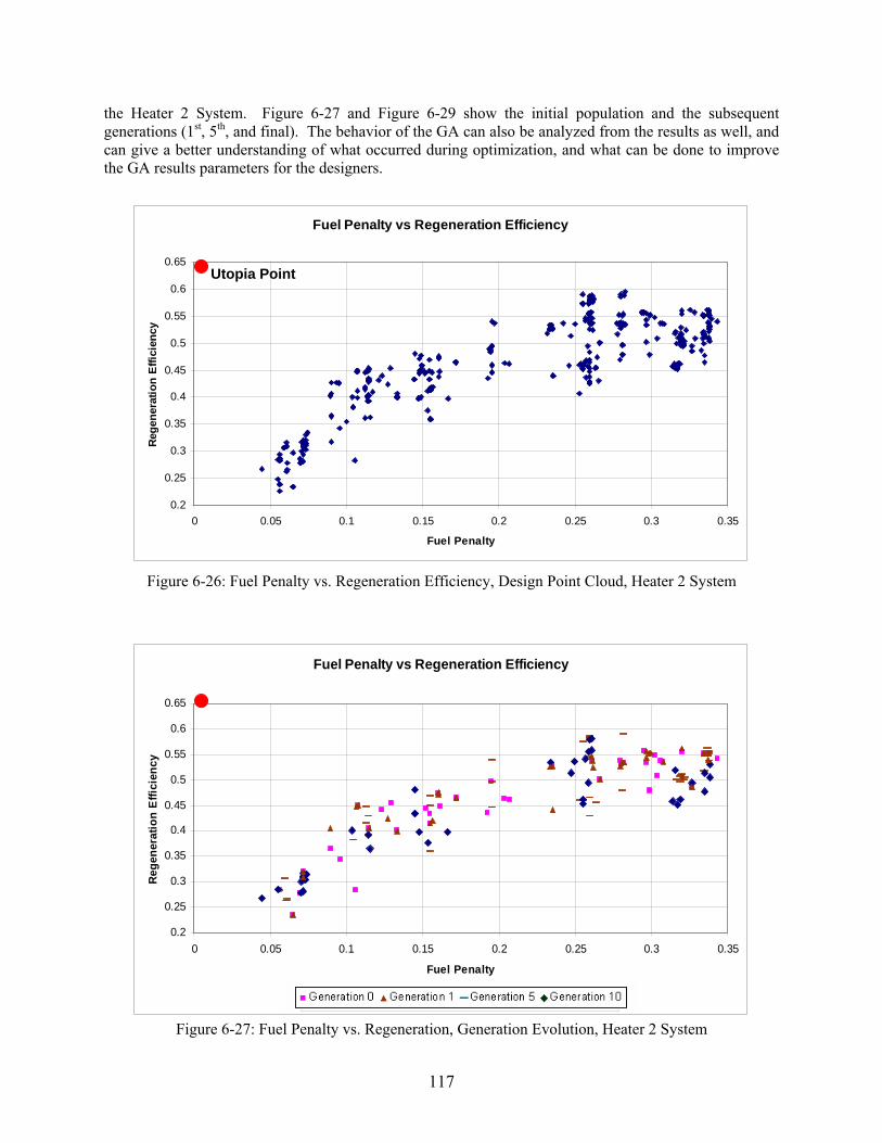
the Heater 2 System. Figure 6-27 and Figure 6-29 show the initial population and the subsequent generations (1st, 5th, and final). The behavior of the GA can also be analyzed from the results as well, and can give a better understanding of what occurred during optimization, and what can be done to improve the GA results parameters for the designers.
Fuel Penalty vs Regeneration Efficiency
0.2
0.25
0.3
0.35
0.4
0.45
0.5
0.55
0.6
0.65
0 0.05 0.1 0.15 0.2 0.25 0.3 0.35
Fuel Penalty
Rege
nera
tion
Effic
ienc
y
Utopia Point
Figure 6-26: Fuel Penalty vs. Regeneration Efficiency, Design Point Cloud, Heater 2 System
Figure 6-27: Fuel Penalty vs. Regeneration, Generation Evolution, Heater 2 System
Fuel Penalty vs Regeneration Efficiency
0.2
0.25
0.3
0.35
0.4
0.45
0.5
0.55
0.6
0.65
0 0.05 0.1 0.15 0.2 0.25 0.3 0.35
Fuel Penalty
Rege
nera
tion
Effi
cien
cy
Generation 0 Generation 5 Generation 10 Generation 1
117
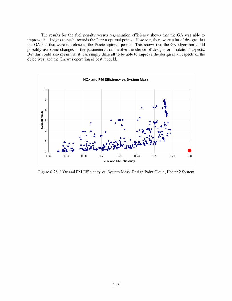
The results for the fuel penalty versus regeneration efficiency shows that the GA was able to
improve the designs to push towards the Pareto optimal points. However, there were a lot of designs that the GA had that were not close to the Pareto optimal points. This shows that the GA algorithm could possibly use some changes in the parameters that involve the choice of designs or “mutation” aspects. But this could also mean that it was simply difficult to be able to improve the design in all aspects of the objectives, and the GA was operating as best it could.
Figure 6-28: NOx and PM Efficiency vs. System Mass, Design Point Cloud, Heater 2 System
NOx and PM Efficiency vs System Mass
3
4
5
6
Syst
em M
ass
0
1
0.64 0.66 0.68 0.7 0.72 0.74 0.76 0.78 0.8
NOx and PM Efficiency
2
118

Figure 6-29: NOx and PM Efficiency vs. System Mass, Generation Evolution, Heater 2 System
NOx and PM Efficiency vs System Mass
0
1
2
3
4
5
6
0.64 0.66 0.68 0.7 0.72 0.74 0.76 0.78 0.8
NOx and PM Efficiency
Syst
em M
ass
Generation 0 Generation 1 Generation 5 Generation 10
The results for the NOx and PM efficiency versus system mass show that the GA was ab le to have its population evolve and improve system mass for the same emission efficiency in the initial generations (from the 1st through the 5th). Also, there were some designs at the higher end of the system mass that the GA found that allowed for better emission efficiency objective at later generations (5th and 10th). Unfortunately, the GA was not able to successively move closer to the Pareto Front through successive generations, but it was able to explore the trade-space well enough to allow a Pareto Front to be resolved from the entire population and generation set.
6.7.2 Dosing System Pareto Fronts in Objective Space The dosing system solutions show that on the system level, there are only two sets of significantly competing objectives. These include: the NOx and PM Efficiency vs. System Mass; and the Fuel Penalty vs. Regeneration Efficiency. The diagrams of these sets of objectives are shown in Figure 6-30 thru Figure 6-31, with only the non-dominated Pareto Optimal Points plotted. It would appear that from these results there appears to be a slight increase in NOx and PM emission conversion efficiency with an increase in system mass. However the normalized mass results show that the increase in mass required for a small increase in efficiency goes into an user-defined infeasible design region, where the increase in mass is more than 50% the amount of the current baseline system (see Section 6.6).
119
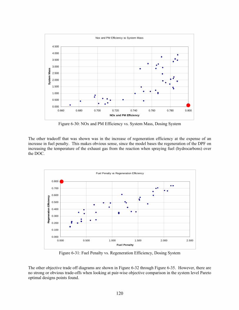
Figure 6-30: NOx and PM Efficiency vs. System Mass, Dosing System
The other tradeoff that was shown was in the increase of regeneration efficiency at the expense of an increase in fuel penalty. This makes obvious sense, since the model bases the regeneration of the DPF on increasing the temperature of the exhaust gas from the reaction when spraying fuel (hydrocarbons) over the DOC.
Figure 6-31: Fuel Penalty vs. Regeneration Efficiency, Dosing System
The other objective trade off diagrams are shown in Figure 6-32 through Figure 6-35. However, there are no strong or obvious trade-offs when looking at pair-wise objective comparison in the system level Pareto optimal designs points found.
Nox and PM Efficiency vs System Mass
4.500
3.000
0.000
0.500
1.000
1.500
2.000
2.500
0.660 0.680 0.700 0.720 0.740 0.760 0.780
Sys
tem
M
3.500
4.000
0.800
NOx an PM Efficiency
ass
d
Fuel Penalty vs Regeneration Efficiency
0.300
0.400
0.500
0.600
0.700
0.800
0.000 0.500 1.000 1.500 2.000 2.500
Fuel Penalty
gene
ratio
n Ef
ficie
ncy
0.000
0.100
0.200Re
120
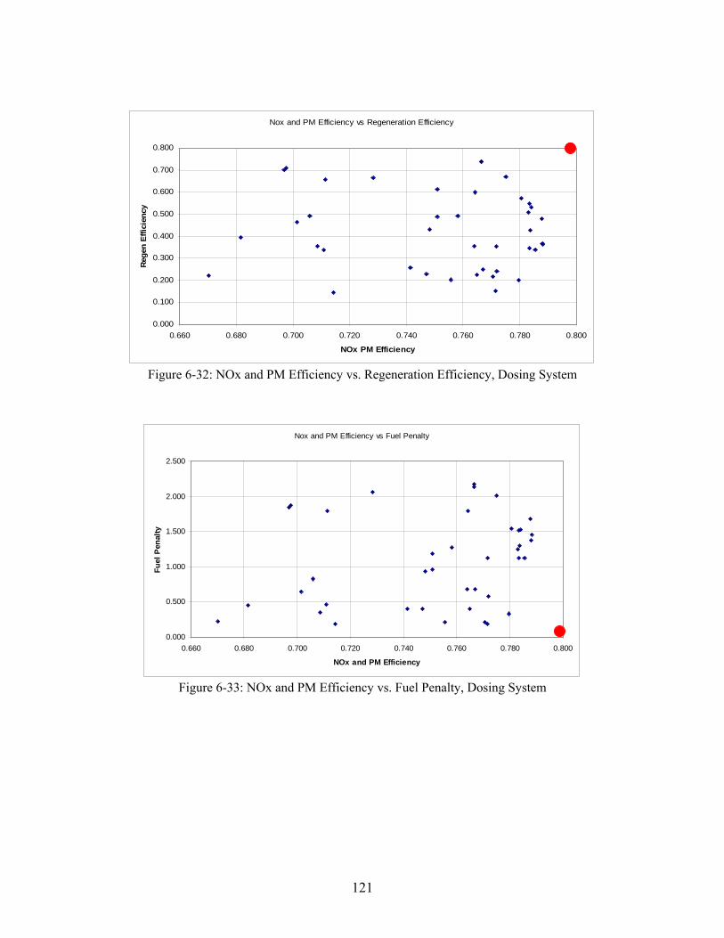
Figure 6-32 stem
Nox and PM Efficiency vs Regeneration Efficiency
0.000
0.100
0.200
0.300
0.400
0.500
0.600
0.700
0.800
0.660 0.680 0.700 0.720 0.740 0.760 0.780 0.800
NOx PM Efficiency
Reg
en E
ffici
ency
: NOx and PM Efficiency vs. Regeneration Efficiency, Dosing Sy
Figure 6-33: NOx and PM Efficiency vs. Fuel Penalty, Dosing System
Nox and PM Efficiency vs Fuel Penalty
0.000
0.500
1.000
1.500
2.000
2.500
0.660 0.680 0.700 0.720 0.740 0.760 0.780 0.800
NOx and PM Efficiency
Fuel
Pen
alty
121
Fuel Penalty vs System Mass
0.000
0.500
1.000
1.500
2.000
2.500
3.000
3.500
4.000
4.500
0.000 0.500 1.000 1.500 2.000 2.500
Fuel Penalty
Syst
em M
ass
Figure 6-34: Fuel Penalty vs. System Mass, Dosing System
Figur em
Regeneration Efficiency vs System Mass
0.000
0.500
1.000
1.500
2.000
2.500
3.000
3.500
4.000
4.500
0.000 0.100 0.200 0.300 0.400 0.500 0.600 0.700 0.800
Regeneration Efficiency
Syst
em M
ass
e 6-35: Regeneration Efficiency vs. System Mass, Dosing Syst
122
6.7.3 Heater 1 System Pareto Fronts in Objective Space
The Heater 1 system solutions show that on the system level, there are 3 sets of competing objectives, including: the NOx and PM Efficiency vs. Fuel Penalty, the NOx and PM Efficiency vs. System Mass; and the Fuel Penalty vs. Regeneration Efficiency. The diagrams of these sets of objectives are shown in Figure 6-36 through Figure 6-38. Some tradeoffs from the design points are illustrated, with the NOx and PM emission conversion efficiency seems to increase, but at the expense of higher fuel usage (or increased fuel penalty). As opposed to the dosing system architecture, this trade-off is more apparent in the heater systems. Additionally, the system mass versus NOx and PM Efficiency tradeoff and the Fuel Penalty and Regeneration Efficiency tradeoffs are apparent. Compared to the dosing system, the design points in the Pareto optimal system set appear to be more clustered and well defined in the pair-wise objective comparison.
Figure 6-36: NOx and PM Efficiency vs. Fuel Penalty, Heater 1 System
Nox and PM Efficiency vs Fuel Penalty
0.1
0.2
0.25
0.3
0.35
0.4
0.72 0.74 0.76 0.78 0.8
Fuel
Pen
alt
0.15
0
0.05
0.66 0.68 0.7
NOx and PM Efficiency
y
123

Figure 6-37: NOx and PM Efficiency vs. System Mass, Heater 1 System
fo
Similar t n mass required r a small increase in efficiency goes into a user-defined infeasible design region, where the increase in
mass is more than 50% the amount of the current stem. However, the knee of the trade-off curve
o the dosing system, the normalized mass results show that the increase i
syappears to be more optimal than the dosing system (with a better conversion efficiency performance for similar normalized system mass).
Figure 6-38: Fuel Penalty vs. Regeneration Efficiency, Heater 1 System
Nox and PM Efficiency vs System Mass
0
1
2
3
4
5
6
0.66 0.68 0.7 0.72 0.74 0.76 0.78 0.8
NOx and PM Efficiency
Syst
em M
ass
Fuel Penalty vs Regeneration Efficiency
0
0.
0.2
0.3
0.4
0.5
0.6
0.7
0 0.05 0.1 0.15 0.2 0.25 0.3 0.35 0.4
Reg
ener
atio
n Ef
ficie
nc
1
Fuel Penalty
y
124
6.7.4 Heater 2 System Pareto Fronts in Objective Space The second heater system solutions show that on the system level, there are only 3 sets of
; The NOx and PM Efficiency vs. System Mass; and the Fuel Penalty vs. Regeneration Efficiency. The diagrams of these sets of objectives are shown in Figure 6-39 through Figure 6-41. Although, the other sets of objectives did not show significant trade-offs, that does not discount the possibility that they would exist in other architectures or designs.
significantly competing objectives. These include: the NOx and PM Efficiency versus Fuel Penalty
Nox and PM Efficiency vs Fuel Penalty
0.050
0.100
0.150
0.200
0.250
0.300
0.350
0.400
Fuel
Pen
alty
0.0000.640 0.660 0.680 0.700 0.720 0.740 0.760 0.780 0.800
NOx and PM Efficiency
Figure 6-39: NOx and PM Efficiency vs. Fuel Penalty, Heater 2 System
125

Figure 6-40: NOx and PM Efficiency vs. System Mass, Heater 2 System
Nox and PM Efficiency vs System Mass
0.000
1.000
2.000
3.000
4.000
5.000
6.000
0.640 0.660 0.680 0.700 0.720 0.740 0.760 0.780 0.800
NOx and PM Efficiency
Syst
em M
ass
Fuel Penalty vs Regeneration Efficiency
0.000
0.100
0.200
0.300
0.400
0.500
0.600
0.700
0.000 0.050 0.100 0.150 0.200 0.250 0.300 0.350 0.400
Fuel Penalty
Reg
ener
atio
n Ef
ficie
ncy
Figure 6-41: Fuel Penalty vs. Regeneration Efficiency, Heater 2 System
126

6.7.5 Comparison of Objective Space Tradeoffs Between System Architectures
The overall performance of the three different system architectures (Figure 6-42) in terms of NOx
and PM Efficiency and System Mass isn’t widely different. For system mass objective values under 1.0, all three systems seem to offer a similar performance Pareto curves. However, at higher system mass objective values, those over 1.5, the Pareto Fronts of the system are rather different. The Dosing System seems to benefit the most from higher system masses, with the Heater 1 System not far behind. Both of these systems maximize their NOx and PM Efficiencies around 0.790 and 0.785, respectively. The Heater 2 system behaves much differently, where the maximum emission conversion efficiency is near 0.770, lower than the other two systems. The Pareto Front appears to be slightly better, however, at lower system masses. In particular, there are a number of design points between the values of 0.710 and 0.740 for the NOx and PM Efficiency objective where the system mass is significantly less for the Heater 2 system versus the other two system architectures. It is important to note that overall, the behavior for all three system architectures is very similar for the tradeoff between mass (or cost) and NOx and PM Efficiency, with the exception of the slightly poorer performance of the Heater 2 system for the more massive system designs. The other major objective tradeoff that was resolved for each architecture (Fuel Economy Penalty vs. Regeneration Efficiency in Sections 6.7.2 through 6.7.4) showed a much different result between the systems (see Figure 6-43).
After identifying the three significant pair-wise objective trade-offs for each system architecture
case, the next step is to overlay the Pareto Fronts of each system for each objective trade-off. This comparison allows designers and engineers to be able to directly compare the different architectures’ behaviors and trade-offs, which allows for a better understanding of the nature of the systems involved.
NOx and PM Efficiency vs System Mass
0.000
0.500
1.000
1.500
2.000
2.500
3.000
3.500
4.000
4.500
5.000
790
Syst
em M
ass
0.650 0.670 0.690 0.710 0.730 0.750 0.770 0.
NOx and PM Efficiency
Dosing System Heater 1 System Heater 2 System
Heater 2 Pareto Front Estimate
Heater 1 Pareto Front Estimate
Doser Pareto Front Estimate
Figure 6-42: NOx and PM Efficiency vs. System Mass for Three System Architectures
127
Figure 6-43: Fuel Economy Penalty vs. Regeneration Efficiency for Three System Architectures
Fuel Economy Penalty vs Regeneration Efficiency
0.000
0.100
0.200
0.300
0.400
0.500
0.600
0.700
0.800
0.000 0.200 0.400 0.600 0.800 1.000 1.200 1.400 1.600 1.800 2.000
Fuel Economy Penalty
Rege
nera
tion
Effi
cien
cy
Dosing System Heater 1 System Heater 2 System
Heater 2 Pareto Front Estimate
Heater 1 Pareto Front Estimate
Doser Pareto Front Estimate
The Dosing System had a very well defined Pareto Front, but with fuel economy penalty
Also, there were other differences in the heater systems that merit review. The most important one is that the Heater 2 System has generally worse emission performance than the Heater 1 System. This is due to the fact that the hydrocarbon slip that occurs in the combustor is allowed to pass downstream out the tailpipe instead of being flowed into a DOC where it can be oxidized. These hydrocarbon emissions can be significant.
objective values ranging between 0.200 to 2.000. The fuel economy penalty value of 1.0 means that the system requires approximately 10% on top of the fuel used to run the engine to regenerate the DPF. With regeneration efficiencies around 50%, the system is right near the fuel economy penalty value of 1.0, which is the most fuel economy penalty that is generally accepted by commercial operators. The heater systems both performed far better than the dosing system with respect to the fuel economy penalty versus the regeneration efficiency. In most cases, both systems were using nearly an order of magnitude less fuel than the dosing systems to achieve the same regeneration efficiencies. The significant improvement in performance here, even when looking at this as a tradeoff, means that designers have found a fundamental performance difference between the system architectures. Overall, the three different system architectures behave very similarly to each other in terms of performance tradeoffs in their objectives. However, a significant difference in actual values occurs in the fuel economy versus regeneration efficiency trade-off, where it appears that a Heater/Combustor system has an inherent performance gain compared to a dosing system.
128
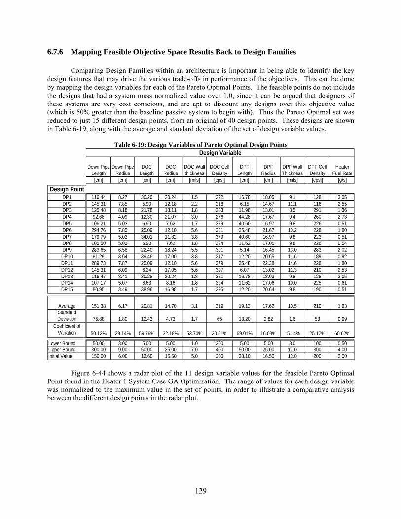
6.7.6 Mapping Feasible Objective Space Results Back to Design Families Comparing Design Families within an architecture is important in being able to identify the key design features that may drive the various trade-offs in performance of the objectives. This can be done by mapping the design variables for each of the Pareto O
ystem mass normalized value ptimal Points. The feasible points do not include
the designs that had a s over 1.0, since it can be argued that designers of these systems are very cost consci ny designs over this objective value (which is 50% greater than the base th). Thus the Pareto Optimal set was reduced to just 15 different design points, from an original of 40 design points. These designs are shown in Table 6-19, along with the average and standard deviation of the set of design variable values.
Table 6-19: Design Variables of Pareto Optimal Design Points
DOC DOC Wall DOC Cell DPF Length
DPF Radius
DPF Wall Thickness
DPF Cell Density
Heater Fuel Rate
[cm] [cm] [cm] [cm] [cm] [mils] [cpsi] [g/s]
Desi
ous, and are apt to discount aline passive system to begin wi
Down Pipe Length
Down Pipe Radius
DOC Length Radius thickness Density
[cm] [mils] [cpsi]
gn PointDP1 116.44 8.27 30.20 20.24 1.5 222 16.78 18.05 9.1 128 3.05DP2 145.31 7.85 5.90 12.18 2.2 218 6.15 14.67 11.1 116 2.55DP3 125.48 8.18 21.78 18.11 1.8 283 11.98 13.01 8.5 291 1.36DP4 92.68 4.09 12.30 21.07 3.0 276 44.28 17.67 9.4 260 2.73DP5 106.21 5.03 6.90 7.62 1.7 379 40.60 16.97 9.8 226 0.51DP6 294.76 7.85 25.09 12.10 5.6 381 25.48 21.67 10.2 228 1.80
DP9 283.65 6.58 22.40 18.24 5.5 391 5.14 16.45 13.0 283 2.02DP10 81.29 3.64 39.46 17.00 3.8 217 12.20 20.65 11.6 189 0.92
1
Average 151.38 6.17 20.81 14.70 3.1 319 19.13 17.62 10.5 210 1.63and
4.00itial Value 150.00 6.00 13.60 15.50 5.0 300 38.10 16.50 12.0 200 2.00
Design Variable
DP7 179.79 5.03 34.01 11.82 3.8 379 40.60 16.97 9.8 223 0.51DP8 105.50 5.03 6.90 7.62 1.8 324 11.62 17.05 9.8 226 0.54
DP 1 289.73 7.87 25.09 12.10 5.6 379 25.48 22.38 14.6 228 1.80DP12 145.31 6.09 6.24 17.05 5.6 397 6.07 13.02 11.3 210 2.53DP13 116.47 8.41 30.28 20.24 1.8 321 16.78 18.03 9.8 128 3.05DP14 107.17 5.07 6.63 8.16 1.8 324 11.62 17.06 10.0 225 0.61DP15 80.95 3.49 38.96 16.98 1.7 295 12.20 20.64 9.8 190 0.51
St ard Deviation 75.88 1.80 12.43 4.73 1.7 65 13.20 2.82 1.6 53 0.99
Coefficient of Variation 50.12% 29.14% 59.76% 32.18% 53.70% 20.51% 69.01% 16.03% 15.14% 25.12% 60.62%
Lower Bound 50.00 3.00 5.00 5.00 1.0 200 5.00 5.00 8.0 100 0.50Upper Bound 300.00 9.00 50.00 25.00 7.0 400 50.00 25.00 17.0 300In
Figure 6-44 shows a radar plot of the 11 design variable values for the feasible Pareto Optimal Point found in the Heater 1 System Case GA Optimization. The range of values for each design variable was normalized to the maximum value in the set of points, in order to illustrate a comparative analysis
etween the different design points in the radar plot. b
129
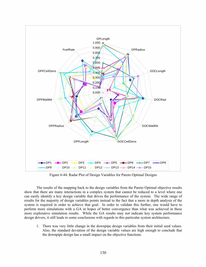
0.000
0.100
0.200
0.300
0.500
0.600
0.700
0.800
0.900
1.000DPLength
DPRadiusFuelRate
0.400 DOCLength
DOCRad
DOCWallthk
DOCCellDensDPFLength
DPFRadius
DPFWallthk
DPFCellDens
DP1 DP2 DP3 DP4 DP5 DP6 DP7 DP8DP9 DP10 DP11 DP12 DP13 DP14 DP15
Figure 6-44: Radar Plot of Design Variables for Pareto Optimal Designs
The results of the mapping back to the design variables from the Pareto Optimal objective results
order to validate this further, one would have to erform more simulations with a GA in hopes of better convergence than what was achieved in these
more explorative simulation results. While the GA results may not indicate key system performance design drivers, it still leads to some conclusions with regards to this particular system architecture.
1. There was very little change in the downpipe design variables from their initial seed values. Also, the standard deviation of the design variable values are high enough to conclude that the downpipe design has a small impact on the objective functions.
show that there are many interactions in a complex system that cannot be reduced to a level where one can easily identify a key design variable that drives the performance of the system. The wide range of results for the majority of design variables points instead to the fact that a more in depth analysis of the system is required in order to achieve that goal. Inp
130

2. The DOC length appears to have grown from the initial value, and the radius has been kept nearly the same. However, the standard deviation of the length variable is very high.
3. The DOC wall thickness variable has generally shown to be smaller than the initial seed, and
the cell density generally trends to a higher value. This corresponds to the current drive towards thinner wall, higher density monolith substrates which leads to higher DOC efficiencies.
4. The DPF length variable generally trended lower, but still with a high standard deviation.
The DPF radius was not changed significantly from the initial value. 5. Similar to the DOC, the DPF wall thickness and cell density trended towards thin-wall and
high density substrates. 6. Logically, the heater fuel rate was generally reduced in the optimization to lower values than
the original specification.
6.7.7 Comparing Aspect Ratios between DOCs and DPFs
In terms of architecture, one characteristic that is used in designing the system is the aspect ratio of the DOC and DPF, where aspect ratio is defined as length to diameter. This is important in terms of packaging a system design within a vehicle, and engineers can use the optimization to find the appropriate design direction that will lead to better performing systems. In the DOC case study in prior sections, it was shown that a generally higher aspect ratio (long, tubular catalyst shapes as opposed to shorter “pancake-like” shapes) performed better for overall emission efficiency. However, in this case, a wider variety of aspect ratios appeared. Example aspect ratio visualizations are shown in Figure 6-45.
Figure 6-45: Aspect Ratio Comparisons
L = D/3
D
AR = 1/3
D
L = 2DL = 2D
D
AR = 1 AR = 2
Aspect Ratio Examples AR = Length / Diameter
131
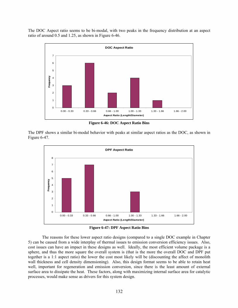
The DOratio of arou
C Aspect ratio seems to be bi-modal, with two peaks in the frequency distribution at an aspect nd 0.5 and 1.25, as shown in Figure 6-46.
DOC Aspect Ratio
6
7
4
5
2
3
0
1
0.00 - 0.33 0.33 - 0.66 0.66 - 1.00 1.00 - 1.33 1.33 - 1.66 1.66 - 2.00
Aspect Ratio (Length/Diameter)
Freq
uenc
y
s
he DP
Figure 6-46: DOC Aspect Ratio Bin T F shows a similar bi-modal behavior with peaks at similar aspect ratios as the DOC, as shown in Figure 6-47.
DPF Aspect Ratio
7
8
1
2
0
3
4
5
6
0.00 - 0.33 0.33 - 0.66 0.66 - 1.00 1.00 - 1.33 1.33 - 1.66 1.66 - 2.00
Aspect Ratio (Length/Diameter)
Freq
uenc
y
Figure 6-47: DPF Aspect Ratio Bins
The reasons for these lower aspect ratio designs (compared to a single DOC example in Chapter
5) can be caused from a wide interplay of thermal issues to emission conversion efficiency issues. Also, cost issues can have an impact in these designs as well. Ideally, the most efficient volume package is a sphere, and re square the overall (that is the more the overall DOC and DPF put together is a 1:1 aspect ratio) the lower the cost most likely will be (discounting the affect of monolith wall thickness and cell density dimensioning). Also, this design format seems to be able to retain heatwell, important for regeneratio ount of externalurface area to dissipate the heat. These factors, along with maximizing internal surface area for catalytic rocesses, would make sense as drivers for this system design.
thus the mo system is
n and emission conversion, since there is the least am
sp
132
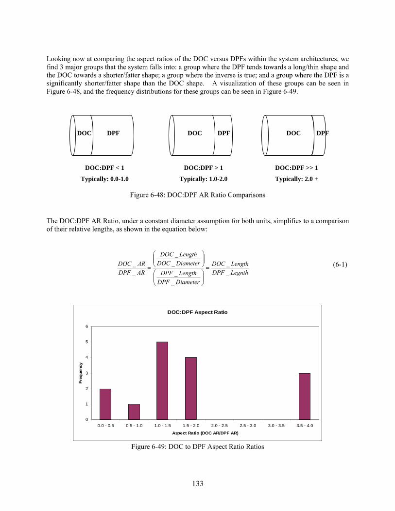
Looking now at comparing the aspect ratios of the DOC versus DPFs within the system architectures, we
nd 3 major groups that the system falls into: a group where the DPF tends towards a long/thin shape and the DOC towards a shorter/fatter shape; a group where the inverse is true; and a group where the DPF is a significantly shorter/fatter shape than the DOC shape. A visualization of these groups can be seen in Figure 6-48, and the frequency distributions for these groups can be seen in Figure 6-49.
Figure 6-48: DOC:DPF AR Ratio Comparisons
e lengths, as shown in the equation below:
fi
The DOC:DPF AR Ratio, under a constant diameter assumption for both units, simplifies to a comparison of their relativ
LegnthDPFLengthDOC
DiameterDPFLengthDPF
DiameterDOCLengthDOC
ARAR
__
__
__
__
=
⎟⎟⎠
⎞⎜⎜⎝
⎛
⎟⎟⎠
⎞⎜⎜⎝
⎛
=
DPFDOC
DOC:DPF < 1
Typically: 0.0-1.0
DOC:DPF > 1
Typically: 1.0-2.0
DOC:DPF >> 1
Typically: 2.0 +
DOC DPF DPF DPF DOC DOC
DOC:DPF Aspect Ratio
0
1
2
0.0 - 0.5 0.5 - 1.0 1.0 - 1.5 1.5 - 2.0 2.0 - 2.5 2.5 - 3.0 3.0 - 3.5 3.5 - 4.0
Aspect Ratio (DOC AR/DPF AR)
3
4
5
6
Freq
uenc
y
Figure 6-49: DOC to DPF Aspect Ratio Ratios
133
(6-1)

Although these results are preliminary, it can be concluded that with the data available, engineers can
derstood that the e rmance was the group of system arch goal was to be the emission conversion efficiency and regeneration capability re closely match those stem and the Heater 1 sy . The best result found via the GA d optimizer. The optimizer
osen was the Mixed Integer Optim iSight. The same esign variables, objectives, and boundary conditions used in the GA Optimization were used in the
ve value and design variable results of the ptimization (and the initial design point, and the starting design point from the GA). In summary, the OST optimizer was able to improve the NOx and PM Efficiency, with small trade off in the Fuel
Economy Penalty objective. Also, the Regeneration Efficiency was increased, and the system mass was decreased from the initial starting point found by the GA. This points to the conclusion that while a GA was useful in exploring the design space, and obtaining valuable information with regards to objective trade-off, a more refined optimizer is required to obtain the optimum solution. Within this local area, we an be confident that the MOST optimizer found the optimal solution. However, we cannot be assured at given the wide expanse of the design space that this is indeed the true global optimum, especially
given the results shown in the GA; more computation would be required.
Table 6-20: Objective Values for Heater 2 System Designs Pre- and Post- Optimization Architecture \ Average
Objective Result Avg_eff NOx &
PM Eff Fuel Econ. Penalty
Regen capable
Regen Eff
DOC Mass
DPF Mass
System Mass
make design decisions based on the objective performance tradeoffs. For example, if space requirements allow for only very short DPF/DOC combinations, then looking at design points where the aspect ratios are small can lead to different designs that perform well, but that can fit within design packaging constraints.
6.8 Objective Space Refinement Results Validating the second step of the optimization includes choosing a design family from the coarse optimization of an architecture and then refining the results using a gradient based algorithm. For this example, the Heater 2 System Architecture was chosen because of its low system mass and minimal fuel economy penalty. It was un missions perfo worst out of the
itectures, but the to mo
able to improve of the dosing sy stem
in Section 6.7 was refined through a gradient baseization Algorithm [6, 13, 34], as implemented inch
drefinement.
Table 6-20 and Table 6-21 show the objecti oM
cth
Passive Design (Initial) 0.613 0.742 0 0.150 0.130 0.666 0.667 0.666
Heater 2 Design (Start) 0.478 0.668 0.107 0.714 0.449 0.058 0.045 0.101 Heater 2 Design (Best) 0.512 0.716 0.109 0.785 0.498 0.026 0.009 0.061 Objective Function Improvement
7.1% Better
7.2% Better
1.9% Worse
9.9% Better
10.9% Better
55.1% Better
80.0% Better
39.6% Better
The dramatic improvements in System Mass were achieved by basically making the DPF significantly smaller than before. This was doable due to the fact that the system could regenerate the DPF successfully very often, and had high regeneration efficiencies. The DOC mass was further reduced again by making it overall sm y, the system also improved
generation efficiency. Also, the s aller. With a slight more cost in fuel econom
ystem improved emission conversion efficiencies slightly.re
134
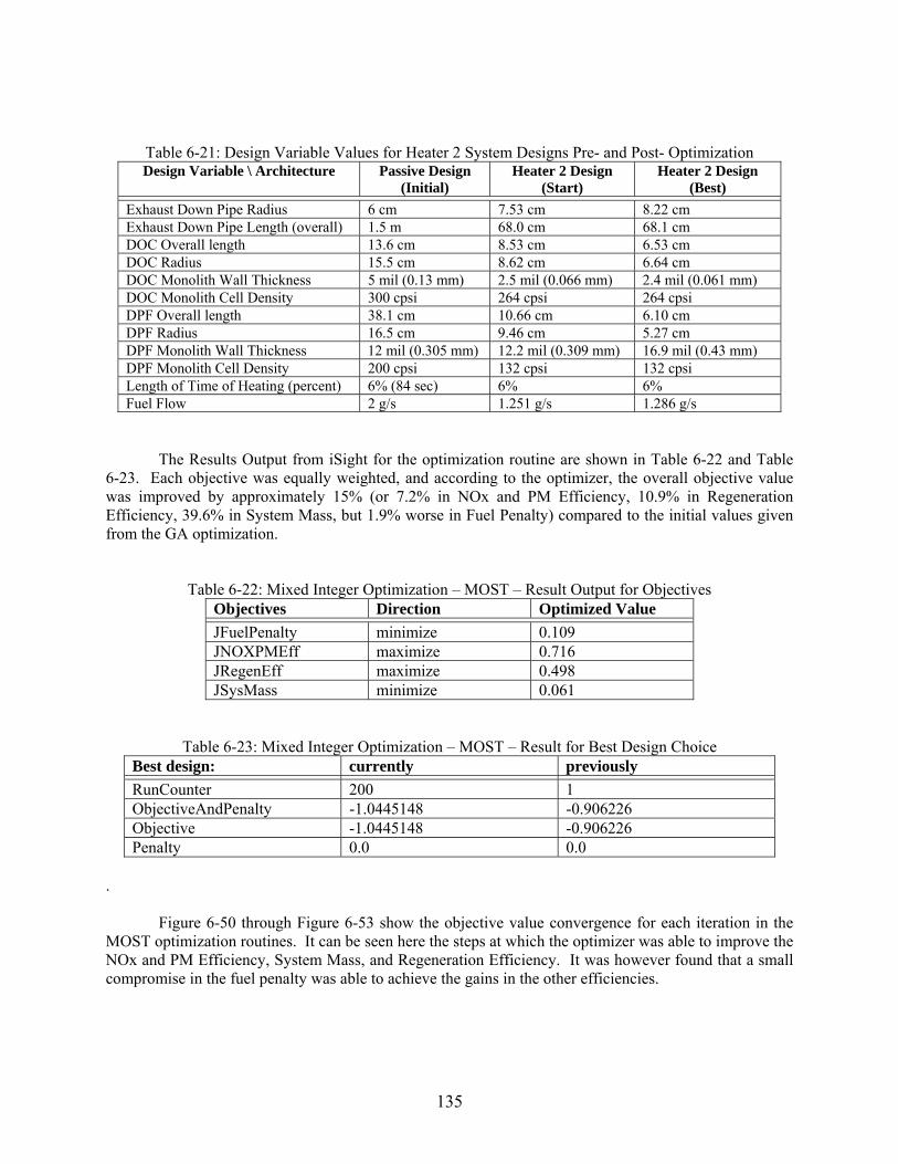
Table 6-21: Design Variable Values for Heater 2 System Designs Pre- and Post- Optimization Design Variable \ Architecture Passive Design Heater 2 Design Heater 2 Design
(Initial) (Start) (Best)
Exhaust Down Pipe Radius 6 cm 7.53 cm 8.22 cm Exhaust Down Pipe Length (overall) 1.5 m 68.0 cm 68.1 cm DOC Overall length 13.6 cm 8.53 cm 6.53 cm DOC Radius 15.5 cm 8.62 cm 6.64 cm DOC Monolith Wall Thickness 5 mil (0.13 mm) 2.5 mil (0.066 mm) 2.4 mil (0.061 mm) DOC Monolith Cell Density 300 cpsi 264 cpsi 264 cpsi DPF verall length 38.1 cm 10.66 cm 6.10 cm ODPF Radius 16.5 cm 9.46 cm 5.27 cm DPF Monolith Wall Thickness 12 mil (0.305 mm) 12.2 mil (0.309 mm) 16.9 mil (0.43 mm) DPF Monolith Cell Density 200 cpsi 132 cpsi 132 cpsi Length of Time of Heating (percent) 6% (84 sec) 6% 6% Fuel Flow 2 g/s 1.251 g/s 1.286 g/s
The Results Output from iSight for the optimization routine are shown in Table 6-22 and Table 6-23. Each objective was equally weighted, and according to the optimizer, the overall objective value was improved by approximately 15% (or 7.2% in NOx and PM Efficiency, 10.9% in Regeneration
fficiency, 39.6% in System Mass, but 1.9% worse in Fuel Penalty) compared to the initial values given the
Efrom GA optimization.
Table 6-22: Mixed Integer Optimization – MOST – Result Output for Objectives Objectives Direction Optimized Value
JFuelPenalty minimize 0.109 JNOXPMEff maximize 0.716 JRegenEff maximize 0.498 JSysMass minimize 0.061
Table 6-23: Mixed Integer Optimization – MOST – Result for Best Design Choice Best design: currently previously
RunCounter 200 1 ObjectiveAndPenalty -1.044514 -0.906226 8 Objective -1.044514 06226 8 -0.9Penalty 0.0 0.0
.
Figure 6-50 through Figure 6-53 show the objective value convergence for each iteration in the OST optimization routines. It can be seen here the steps at which the optimizer was able to improve the M
NOx and PM Efficiency, System Mass, and Regeneration Efficiency. It was however found that a small compromise in the fuel penalty was able to achieve the gains in the other efficiencies.
135

0.66
0.67
0.68O
0.69XPM
Ef 0.7
0.72
0 50 100 200
RunCount
0.71
150 250
er
JNf
Figure 6-50: N M Efficie tive Trace
Ox and P ncy Objec
0.10720.10740.10760.10780.108
50 0 150 0 250
unCounter
JFue
l 0.10820.10840.10860.10880.109
0.10920.1094
Pena
lty
0 10 20
R
Figure 6- nalty Objectiv 51: Fuel Pe e Trace
0.51
0.45
0.46
0.47
0.48
0.5
JReg
enE
0.49
ff
0.440 50 100 150 200 250
RunCounter
Figure 6-52: Regeneration Efficiency Objective Trace
136

0
0.02
0.04
0.06
0.08
0.1
0.12
0 50 100 150 200 250
RunCounter
JSys
Mas
s
Figure 6-53: System Mass Objective Trace
It is useful now to compare the results for the Heater 2 Design versus the initial passive system. Table 6-24 shows the comparison in objective function values between the two systems.
Table 6-24: Objective Values for Heater 2 System Designs Pre- and Post- Optimization Architecture \ Average
Objective Result Avg_eff NOx &
PM Eff Fuel Econ. Penalty
Regen capable
Regen Eff
DOC Mass
DPF Mass
System Mass
Passive Design (Initial) 0.613 0.742 0 0.150 0.130 0.666 0.667 0.666
Heater 2 Design (Best) 0.512 0.716 0.109 0.785 0.498 0.026 0.009 0.061
Percent Difference in Objective Function Value
16.5% Worse
3.5% Worse
N/A 423.3% Better
283.1% Better
96.1% Better
98.6% Better
90.8% Better
The regeneration capab stem mass (cost) performances
l were markedly improved over the initial passive system. The Heater 2 Design allows for a much aller DOC/DPF unit to be used, with smaller margin for particulate matter storage because of its ability
to more successfully regenerate more often. However, this good regeneration behavior comes at a cost. The hydrocarbon emissions associated with the heater/combustor unit can lead to significantly worse overall emissions performance. This was shown with a 16.5% worse average emission conversion efficiency objective value, which begs the question if the design still meets regulations and if there are any changes that are required for this to occur. However, the NOx and PM conversion efficiency objective value was only 3.5% worse. The reason for this can be the fact that with more regenerations occurring, even though the particulate mass can be more successfully burned, the fact remains that there will always be some inefficiencies associated with this process that will release some more particulate mass than would happen if the particulate filter was only storing particulates. These tradeoffs, however, were minimized by using an optimization routine to find the best overall balance of objectives. There is a point to be made that given better combustor design for the heater system, better emission performance on a system level can occur. Part of the heater system design that was modeled was the hydrocarbon slip past the combustor, which was assumed to be about 5% of the total hydrocarbons injected. I missions conversion can
ccur. If this cannot be im s Heater 1 System, where e heater/combustor is upstream of the DOC would potentially be a better decision.
ility, the regeneration efficiency, and the syalsm
f this efficiency can be improved, then better overall eproved, then changing the system architecture towardo
th
137
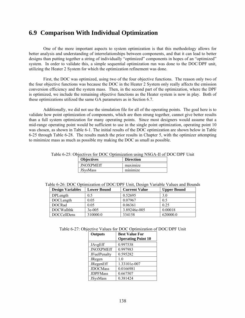
6.9 Comparison With Individual Optimization
One of the more important aspects to system optimization is that this methodology allows for
better analysis and understanding of interrelationships between components, and that it can lead to better designs than putting together a string of individually “optimized” components in hopes of an “optimized” system. In order to validate this, a simple sequential optimization run was done to the DOC/DPF unit, utilizing the Heater 2 System for which the optimization refinement was done.
First, the DOC was optimized, using two of the four objective functions. The reason only two of
the four objective functions was because the DOC in the Heater 2 System only really affects the emission conversion efficiency and the system mass. Then, in the second part of the optimization, where the DPF is optimized, we include the remaining objective functions as the Heater system is now in play. Both of these optimizations utilized the sam
Additionally, we did not use the simulation file for all of the operating points. The goal here is to
alidate how point optimization of components, which are then strung together, cannot give better results
n, operating point 10 as chosen, as shown in Table 6-1. The initial results of the DOC optimization are shown below in Table
6-25 thro empting to h le DO all ib
: Objectives fo O NSGA-II of
e GA parameters as in Section 6.7.
vthan a full system optimization for many operating points. Since most designers would assume that a mid-range operating point would be sufficient to use in the single point optimizatiow
ugh Table 6-28. The results match the prior results in Chapter 5, with the optimizer att minimize mass as muc as possib my making the C as sm as poss le.
Table 6-25 r DOC ptimization using DOC/DPF Unit Objectives Direction
JNOXPM maxEff imize JSysMas mins imize
Table 6-26: DOC Optimization of DOC/DPF Unit, Design Variable Values and Bounds Design Variables Lower Bound Current Value Upper Bound
DPLength 0.5 0.52695 3.0 DOCLength 0.05 0.07967 0.5 DOCRad 0.05 0.06361 0.25 DOCWallthk 3e-005 3.89246e-005 0.00018 DOCCellDens 310000.0 334158 620000.0
Table 6-27: Objective Values for DOC Optimization of DOC/DPF Unit Outputs Best Value For
Operating Point 10
JAvgEff 0.997538 JNOXPMEff 0.997983 JFuelPenalty 0.595282 JRegen 1.0 JRegenEff 1.33101e-007 JDOCMass 0.0166981 JDPFMass 0.667507 JSysMass 0.381424
138
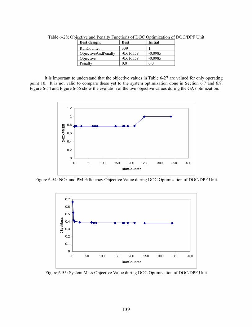
Table 6-28: Objective and Penalty Functions of DOC Optimization of DOC/DPF Unit
Best design: Best Initial
RunCounter 339 1 ObjectiveAndPenalty -0.616559 -0.0985 Objective -0.616559 -0.0985 Penalty 0.0 0.0
It is important to understand that the objective values in Table 6-27 are valued for only operating point 10. It is not valid to compare these yet to the system optimization done in Section 6.7 and 6.8. Figure 6-54 and Figure 6-55 show the evolution of the two objective values during the GA optimization.
0
0.2
1.2
0 0 150 0 300 350 400
Run
0.4
0.6
0.8
1
JNO
XPM
Eff
50 10 200 25
Counter
Figure 6-54: NOx and PM Efficiency Objective Value during DOC Optimization of DOC/DPF Unit
0
0.1
0.2
0.3
0 50 0 250 300 350 400
JSys
M
0.4ass
0.5
0.6
0.7
100 15 200
RunCounter
Figure 6-55: System Mass Valu Optimization of DOC/DPF Unit
Objective e during DOC
139

Now we move on to the optimization of the DPF. The technique here was to allow changes to the DPF dime ble 6-29 Table 6-30. Overall, the sa riables as tion 6.7 nsidered.
Table ctives for DP
nsions and the fuel rate of the heater with the rest of the 4 objectives, as shown in Tame design va in Sec were co
6-29: Obje F Optimization of DOC/DPF Unit Objectives Direction
JNOXPMEff maximize JFuelPenalty minimize JRegenEff maximize JSysMass minimize
Table 6-30: DPF Optimization of DOC/DPF Unit, Design Variable Values and Bounds Design Variables Lower Bound Current Value Upper Bound
DPFLength 0.05 0.05265 0.5 DPFRadius 0.05 0.05713 0.25 DPFWallthk 0.00021 0.000308 0.00043 DPFCellDens 155000.0 262131 465000.0 FuelRate 0.5 1.9230 4.0
The results of the optimization are shown in Table 6-31 for the objective function values. These
values are for a simulation only under operating point 10.
Table 6-31: Objective Values for DPF Optimization of DOC/DPF Unit
Outputs Current Value
JAvgEff 0.525828 JNOXPMEff 0.689622 JFuelPenalty 0.127335 JRegen 1.0 JRegenEff 0.614623 JDOCMass 0.031343 JDPFMass 0.00757375 JSysMass 0.0632486
Table 6-32: Objective and Penalty Functions of DPF Optimization of DOC/DPF Unit Best design: currently previously
RunCounter 350 1 ObjectiveAndPenalty -1.1136614 -0.538491 Objective -1.1136614 -0.538491 Penalty 0.0 0.0
ed for nly operatinection 6.7 and 6.8. Figure 6-56 through Figure 6-59 show the evolution of the two objective values
during the GA optimization.
It is important to understand that the objective values in Table 6-31 and Table 6-32 are valug point 10, and it is not valid to compare these yet to the system optimization done in o
S
140

0.66
0.68
0.7
0.72
0.78
0.74
XPM
Ef
0.76
0 200 300 400
RunCounter
JNO
f
100
6-56: NOx and PM Efficiency Objective Value during DPF Optimization of DOC/DPFFigure Unit
0
0.2
0.25
ty
0.05
0.1
JFue
l
0.15
RunCo
Pena
l
0 100 200 300 400
unter
Figure 6-57: Fuel Penal alue duri ptimization of DOC/DPF Unit
ty Objective V ng DPF O
0100
0.10.20.3
JReg
0.40.50.60.7
400
enEf
f
0 200
nCounter
300
Ru
Figure 6-58: Regeneration Efficiency Objective Value during DPF Optimization of DOC/DPF Unit
141
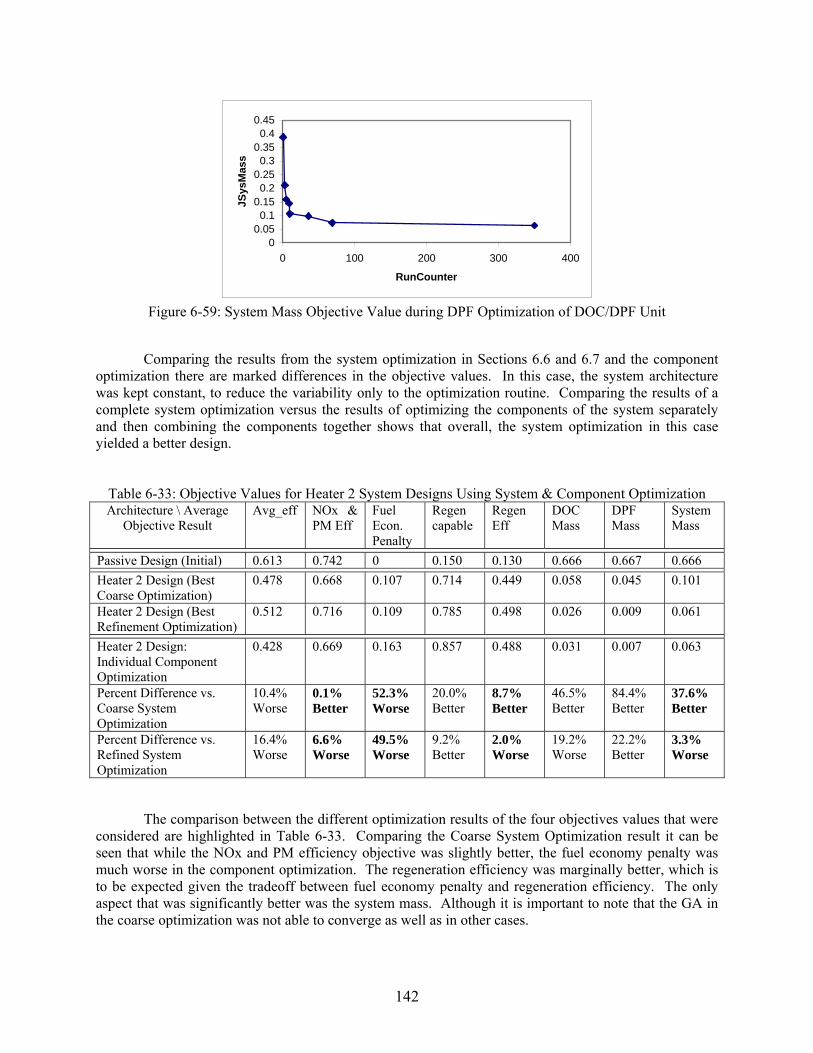
00.050.1
0.150.2
0.250.3
0.350.4
0.45
0 100 200 300 400
RunCounter
JSys
Mas
s
Figure 6-59: System Mass Objective Value during DPF Optimization of DOC/DPF Unit
Comparing the results from the system optimization in Sections 6.6 and 6.7 and the component
ization there are marked differences in the objective values. In this case, the system architecture was kept constant, to reduce the variability only to the optimization routine. Comparing the results of a complete system optimization versus the results of optimizing the components of the system separately and then combining the components together shows that overall, the system optimization in this case yielded a better design.
Table 6-33: Objective Values for Heater 2 System Designs Using System & Component Optimization Architecture \ Average
Objective Result Avg_eff NOx &
PM Eff Fuel Econ. Penalty
Regen capable
Regen Eff
DOC Mass
DPF Mass
System Mass
optim
Passive Design (Initial) 0.613 0.742 0 0.150 0.130 0.666 0.667 0.666
Heater 2 Design (Best Coarse O
0.478 0.668 0.107 0.714 0.449 0.058 0.045 0.101 ptimization)
Heater 2 Design (Best efinement Optimization)
0.512 0.716 0.109 0.785 0.498 0.026 0.009 0.061 R
Heater 2 Design: Individual Component Optimization
0.428 0.669 0.163 0.857 0.488 0.031 0.007 0.063
Percent Difference vs. Coarse System Optimization
10.4% Worse
0.1% Better
52.3% Worse
20.0% Better
8.7% Better
46.5% Better
84.4% Better
37.6% Better
Percent Difference vs. Refined System Optimization
16.4% Worse
6.6% Worse
49.5% Worse
9.2% Better
2.0% Worse
19.2% Worse
22.2% Better
3.3% Worse
The comparison between the different optimization results of the four objectives values that were considered are highlighted in Table 6-33. Comparing the Coarse System Optimization result it can be see as
uch worse in the component optimization. The regeneration efficiency was marginally better, which is to be expected given the tradeoff between fuel economy penalty and regeneration efficiency. The only aspect that was significantly better was the system mass. Although it is important to note that the GA in the coarse optimization was not able to converge as well as in other cases.
n that while the NOx and PM efficiency objective was slightly better, the fuel economy penalty wm
142

Comparing the individual component optimization versus the refined system optimization results shows that the component optimization was worse in every objective that was used for the optimization routine. Additionally, it was worse for the DOC mass and average emission conversion efficiency. The only objective that was better was the regeneration capability and DPF mass. This can be explained because the simulation was run under operating point 10, which even though a mid-range operating point in terms of load and RPM, it allowed for a heater/combustor fueling setting that would allow more successful regeneration attempts at other operating points. Rather than be able to have the optimization algorithm be able to balance between emission efficiency, reducing fuel economy penalty, increasing regeneration efficiency and reducing mass for all of the operating points, the separate component and single-operating point optimization drove a design that may have been very good at that level, but didn’t work well for the overall system and for the entire range of operating points.
.10 Computational Effort
ach operating point (in Matlab), takes approximately 159 seconds.
•
: o
izations with 4 lted on the order of 1 e
: 18 hrs 2 in 17 h in
: 18 h in
eneficial for users to try to limit the size of the simulation input file in order to min n alg s f ur re t
ta po fec va si arc es ount of time. Parallel computing is a solution that can offer to spread the computational
the , si i ile is se oo e e for the tio tio ra nve nd pu can
l effort and maximize the amount of information that can be gained from such optimization imulations.
6 The computational effort is directly dependent on the size of the model file and computations it requires, and the size of the simulation input file. Using a Pentium D CPU 3.2GHz, 3.5GB RAM, 250GB drive, Dell Optiplex GX620 system, and running 1 iteration of a simulation of 20 steady state points, at 1800 seconds of data for e
Dosing System: 159.4 seconds • Heater 1 System: 158.3 seconds • Heater 2 System 158.8 sec nds
Running the GA Optimeach.
40 iterations resu 8 hours of computation tim
• Doser System 6 m
rs 53 m• Heater 1 System: System• Heater 2
It would be b
rs 15 m
obtain less time consuyield the required dareasonable am
g simulations. Run ing optimluate the different sy
ization orithmstem de
or 20 hogns or
s or mohitectur
may nowithin a ol to ef tively e
load, but the root ofappropriate cascomputationa
problemsimula
that ofn condi
mulationns (ope
nput fting e
length,lope) a
still pre the in
nt. Cht file
sing th reduce
s
143
6.11 Summary First, it was concluded that the requirements for successful regeneration capability in this case for a DOC/DPF unit was not possible under a passive system. The problem was that the engine would have to operate at high load and high RPM conditions for an extended period of time to be able to allow for the DPF to regenerate on the vehicle. The reason that DPFs need to be regenerated during the operation of the vehicle is due to the costs associated with having to remove the DPF and clean it off the vehicle manually. This process is time consuming, costly, and leads to significant downtime of a commercial heavy duty vehicle. The downtime issue can be addressed by having a stock of DPFs that can replace full
nits, but this also adds cost, and doesn’t address the labor issues of removal anu d installation. The goal of any commercial heavy duty vehicle operators is to have an online system that can regenerate the DPF
n-road.
he DPF in a satisfactory manner was shown in Section 6.2. rom this, a set of design variables, objective sets, and operating conditions were defined, from which we ould then develop an optimization routine for the DOC/DPF unit. Three different DOC/DPF system
en the three rchitectures was also compared.
eater 2 System was chosen for a more refined optimization, in atte ts emission performance but retain its better fuel economy penalty bjective value, system mass (cost) performance, and regeneration efficiency. This refinement
e system in terms of emission performance. In terms of regeneration behavior and system mass nd thus cost), the Heater 2 System was significantly improved over the passive design, as shown in
Section the results already presented with an attempt to optimize
e D C ndivid ead of system level. In this case, the DOC part e s
izing the entire system on a higher level.
mo The lack of ability to regenerate tFcarchitectures were defined and described, and their baseline results then presented in Section 6.6. A Genetic Algorithm was then used to attempt a coarse optimization of the three systems, in attempts to characterize their behaviors and investigate any significant objective tradeoffs that the designs may have an effect on. These tradeoff results were presented in Section 6.7, and the tradeoffs betwea
From these initial results, the Hmp to improve its relatively worse
ooptimization was able to improve the objective function values to levels that are on par with the initial passiv(a
6.8.
Most significant was the comparison ofO /DPF unit on an i ual component level instth
of th ystem was optimized, and then the DPF part was optimized. The objectives were kept the same overall as before. The only difference was the DOC optimization only required two of the four objectives due to the inherent capability of the DOC relative to the objectives. Also, the simulations were done for only a mid-range operating point to illustrate what single operating point optimization can do to the results. This optimization yielded a design that was good overall. However, it was not as good in terms of the performance objectives as the results from the system optimization in Sections 6.7 and 6.8. This validates one of the major points in the hypothesis: that optimizing components separately and then physically combining them together in hopes of an optimized system may not yield as good performance
vels as optimle
144

Chapter 7
using systems analysis thinking, and a platforming architecture in the o l d
eter inputs. Also, the computational efficiency these models can be significantly better than the more traditional CFD or FEA programs.
. Conclusions After investigating the two case studies in Chapters 5 (Single Component) and 6 (Multi-Component or System), it was found that by applying Systems Analysis and Multidisciplinary Analysis and Design Optimization methodology to the model development and system design of diesel exhaust after-treatment technology can yield valuable insight. The development of a state-vector based system modeling, analysis, and optimization methodology to the design of potentially complex and integrated physical systems has traditionally presented problems in terms of model accuracy and fidelity and omputational issues. However, byc
m de evelopment process, these issues have been addressed. The hypothesis that this methodology can accurately model and investigate different designs, and be able to use optimization to refine designs, has been shown to be valid.
7.1 Validation of Methodology and Approach The main goals of the methodology and approach were to develop a modeling and analysis framework, develop the tools needed for the models, develop and integrate the optimization and analysis tools, and then be able to MSDO to analyze and evaluate the designs and architectures of the exhaust systems. Chapter 3 concerned itself with the approach and development of the modeling framework. It was found that using a state vector as the model platform by which different model architectures can be defined, a variety of different designs can be modeled. These models have the required fidelity to be used as accurate predictive modeling tools, due to the nature of the mathematical models. These models were based in large part on the research and testing results from experts in the field of diesel engine technology. By implementing them in such a way to develop a system model, by which the inputs and outputs become the state vector interface, one can retain the fidelity of the model, and allow for a variety
f different operating conditions, environments, and paramoof
145

7.2 Modularity and Flexibility In addition, the novel approach by which the state vector is used a modeling platform allows for flexibility and modularity in the modeling that mimics the wide vdesigns. Platform architecture has traditionally been used for dapplying it to modeling methodology can yield significant benefitsmodeling technologies, flexibility in operamodularity of different architectures of exh
ariety of possibilities of the physical esign and product development, but . These benefits can be flexibility in
ting conditions used in simulation, modularity of designs, and aust systems.
.2.1 Future Changes
In addition to allowing flexibility in defining designs and architectures for analysis, the plementation of the modeling theory and code allow for straightforward changes in the future.
Changes to the platform, as defined by the list of parameters in the state vector, can allow future
odules to be incorporated on new platforms. Current modules can be easily recoded to allow for use in ew platforms. This allows for minimal effort in implementing new, unforeseen technologies, and thus
y in the modeling and simulation tool.
7
imAlthough there have been placeholders included in the State Vector to allow for future uncertainty in technology modeling, there may be a time where there needs to be more fundamental changes in the State Vector Platform. By viewing the modeling and simulation tool in a manner that divides the platform from the modules and operation inputs, as in Figure 7-1, one can easily visualize various modeling platforms [29, 39].
}Platform
State Vector
}DOC Heater DPF Modules
Engine Model and Vehicle
Configuration
Drive Cycle
Operation Inputs
Figure 7-1: State Vector Platform Mapping
mnallows for flexibilit
146

The state vector platform also defines thnd drive cycle modeling and simulation is con
e data interface with the operation inputs. The engine figured to match the particular state vector platform it
hould there be significant changes in terms of content to the operation inputs, that would necessitate a
.2.2 Cost and Time Savings
It was already established that given the combinatory nature of the components in an exhaust stem,
inations that can be made. If we expand it to include up to 5 different modules in
ebug, and finalize into a robust, polished, coded model. Given the labor effort associated with c d the fact that there would be 31 different models that would be developed from scratch, we can that there will be a learning curve to an engineer developing th s (as per Eq and (
xY
aSchange of the state vector platform. The inverse is true when there is significant change to the state vector platform – the operation inputs would require change to match the new state vector content. In concept, however, using different state vector platforms can help in differentiating different system modeling regimes. For example, there can be a gasoline/electric state vector platform – in addition to the diesel – should there be significant content changes required in this fundamentally different system.
7
sy there are a wide array of different exhaust system architectures that can be made from just a few individual technologies (see Section 3.2). Given this fact, it is good to compare the savings in labor effort that would go in the modeling of exhaust systems using a modular state-vector system design, as opposed to developing models from scratch.
Beginning with a comparison of 5 different technologies, it has already been established that given
3 module locations available in the exhaust system architecture, and with 5 different components, there re 25 different comba
the system architecture, which is possible given the modeling tool presented, we increase the possible combinations of exhaust system architectures to 31.
Each model takes approximately 50-100 hours to derive, code into Matlab/Simulink, d
oding, an assume7-2)) ese model s. (7-1)
nxY ⋅= 0
2loglogb
n =
In the previous equations, Y is equal to the number of hours required to develop ng mY0 is equal to the number of hours required for the first model, x is equal to the current model numdevelopment, and b is equal to the learning curve factor (which we assume to be about 75% in this Graph n gives the results in Figure 7-2 for the time it takes to develop each succemodel. The summation of labor effort for this development case is about 1169 hours.
(7-1)
a worki
ing this equatio
147
(7-2)
odel, ber in case). ssive

Time Spent Coding Successive Traditional Model
80.00
100.00
120.00
nt (h
rs)
0.00
20.00
1 3 5 7 9 11 13 15 17 19 21 23 25 27 29 31
Successive Model Number
40.00Tim
60.00e
Spe
Figure 7-2: Time Spent Coding System Models using Traditional Techniques
modular as possible. But, from the 6 model on, the developer now just has to combine any combination of his/her initial 5 models. No longer does the en
are shown in Figure 7-3, and the total time effort required for this development process is approximately 604 hours.
In the modular approach, we can assume the same initial time effort to develop working models,
but with a higher learning curve factor (90%, i.e. less learning), since the designer would have to put in some more effort into making the code for each model as th
gineer need to develop a model from scratch. And therefore, we step down the length of time required to develop the system model down to 8 hours initially. And this now also has a learning curve, but its effect is much smaller (learning curve factor of 95%), since developing the system model becomes an exercise in effectively copying and pasting component models together. The time results
Time Spent Coding Successive Modular Based Model
0.00
20.00
40.00
60.00
80.00
Tim
e Sp
ent (
hrs)
100.00
120.00
0 5 10 15 20 25 30 35
Successive Model Number
Figure 7-3: Time Spent Coding System Models using Modular Based Techniques
148

The labor savings here account for approximately 565 hours, which given a typical cost per hour ($100) of an engineer to a company can amount to savings of about $55,000 in modeling time effort alone. Costs associated with computation is traditionally low, with much of the modeling able to be done on a single workstation, large arrays of computers that might be required for very fast computation of FEA or CFD analysis are not required. Instead, a personal computer or workstation is sufficient for these models to run satisfactorily. Also, the code was developed in Matlab and Simulink, a software that is readily available and inexpensive to license. Similarly, iSight is inexpensive to license to companies who would use it as a floating license throughout the workplace network. But optimization software is not limited to iSight; since Matlab acts as the modeling engine, other commercial optimization software suites can be used that have interfaces to Matlab.
If the number of exhaust system components increases to 8, and we retain a maximum number of
module slots at 5, we increase the total number of possible combinations to 218. The time spent graphs for 218 successive models are shown in Figure 7-4.
Time Spent Coding Successive Models
0.00
20.00
120.00
0 50 100 150 200 250
Successive Model Number
40.00
60.00
80.00
100.00
Tim
e Sp
ent (
hrs)
Modular Based Modeling Standard Modeling
Figure 7-4: Comparison of Time Spent Coding System Models For this case, our savings can be as much as 2013 hours, or about $200,000. As can be seen, the upfront increase in labor effort more than pays off in the end. In addition, the principle behind developing modeling capability is to be able to reduce costs associated with poor design decisions that can occur early in the development process. Increasing the engineer’s knowledge about a particular system before committing to the costs of development can reduce mistakes and cost overruns later in the development cycle. Modeling also adds value by making the full-scale development and testing stage much less expensive due to fewer required tests. The results of the testing stage capability, in add ion t
are also much more valuable since they feed back into the adding to the modelingo validating a product design. it
149

7.3 Case Study Conclusions The case studies used in the thesis show the validation, first of the capability of the multi-disciplinary system wide modeling and analysis method. As applied to modeling diesel exhaust after treatment systems, it was shown that a simple component was able to be analyzed in such way as to show tradeoffs in cost, performance, and the linking between performance and design variables. Additionally it was shown that the modeling methodology allowed for a variety of differing input operating conditions and parameters, a highly flexible model.
r and had significant interactions. The model was apable of addressing these interactions.
The points to highlight from the thesis hypotheses (Section 1.2):
• The system analysis methodology was able to accurately model diesel exhaust system after-treatment technologies. The calibration required to the models that were developed from well-understood and well-developed physical models was very little. Models that use empirical data and phenomenological modeling techniques may require more calibration depending on operating conditions.
• MSDO Methodology was used to compare and investigate exhaust system architectures. The
multi-component system case study compared three different new system architectures to a baseline system currently in production. Tradeoffs in performance objectives were discovered and could be compared between the different system architectures. Each system had its own strengths and weaknesses, and designers could understand the behaviors of each system from the results obtained.
• The trade-offs for each system architecture could be traced back to the design architectures and
design variables used in each architecture. For example, the tradeoffs between fuel economy penalty and regeneration efficiency can be traced to the amount of fuel used in the dosing spray, and to the amount of fuel required for the heater/combustor systems.
• Design Optimization software was integrated into the simulation code, and was able to analyze
the system architectures and develop designs that improved the system performance objectives.
r system designs were able to be developed than would be possible from optimizing each component individually. Objective function value
and manufacturing.
The case studies also showed how it was possible to use test data to help refine a theoretical model, and then use this calibrated model in a larger and more complex exhaust system. This system ncluded many components that affected each othei
c
• By using the systems analysis approach, bette
differences from 2% to nearly 50% were observed.
• Beneficial and harmful component interactions were uncovered – for example the effect of the hydrocarbon slip in the combustor/heater systems.
Design optimization refinement can be done to the exhaust system and possible design configurations resolved for further testing, implementation,
150
7.4 Future Work In general, the more technological components that can be modeled, the more versatile this modeling and simulation tool can become. Its value in being a state-vector platform concept towards modular models that can be easily added and combined together to form different systems was clearly shown. It would now be the case to continue to add different technological modules to the tool. In addition, more engine and operating data should be used in testing different exhaust system models. This data can be further used to validate the after-treatment technologies used in exhaust systems. Including rchitectures with feedback and active control logic would also be a step towards expanding the
an be added modularly or via different modeling platforms.
One other important future development would be the creation of a graphical user interface. k will ease the learning curve associated
ith new software for engineers, as many engineers use tools such as Matlab (if not Matlab itself) on a dail athese exsystem dels and data become available, there can be more refinement done to the actual phy models. Constants and parameters can be better understood and used. With the feedback tow suse of athe usedevelopto the eand dev tion is a modeling and rapid prototyping shop that can yield the quick turn-round time required for this fast development and validation cycle. Investing in closing the development
cyc wAlthougcosts inthe prod ngineering labor.
acapabilities of the program. Adding regeneration triggering via a pressure sensor in certain architectures is one such example of active control logic. The whole modeling and simulation tool can be expanded further to include engine models, inlet (turbomachinery) models, and even hybrid and gas engine alternatives. All of these different models c Although having the modeling tool developed in Matlab/Simulinw
y b sis, a GUI can make the development of different system architectures and different designs of haust systems much faster. This speed can translate into more and better analyses of different
architectures and designs in the early phases of product development.
As more mosical ard refining models and exhaust system architectures comes a big step in being able to validate the
tool such as this in the actual product development cycle. Engineers should begin to implement of this modeling capability at the beginning of the life cycle of a product – in the early ment period. Then, as this product is developed, designed, and then tested, the data should return ngineers to be able to validate and tune the modeling tools. A valuable addition to any research elopment organiza
ale ith this rapid prototyping loop can yield significant results in future product development.
h this final implementation in industry can be difficult, the rewards can far outweigh the initial terms of less testing required, less costs associated with design and manufacturing changes late in uct life cycle, and even less modeling and computer-aided design and e
151
Bibliography [1] ADVISOR2002, NREL’s ADvanced VehIcle SimulatOR, Software Package, Version 2002,
National Renewable Energy Laboratory, U.S. Department of Energy, Washington D.C., 2002. [2] ArvinMeritor, Inc., Products and Services – Truck, Emissions Solutions.
http://www.meritorhvs.com/ [3] Corning DuraTrap® CO filters. www.corning.com/docs/environmentaltechnologies/co.pdf [4 orning DuraTrap® AT filters. ] C www.corning.com/docs/environmentaltechnologies/at.pdf [5] Freightliner Aftertreatment System 2007 Emissions, Emission Components, Detroit Diesel
Corporation, 2006. http://detroitdieselepa07.com [6] iSIGHT, ver. 9.0.7, Engineous Software, Inc., Cary, NC, 2005. [7 atlab, ver. 6.5, release 13, The MathWorks, Inc., Natick, MA, 2002. [8] Simulink, ver. 5.0, The MathWorks, Inc., Natick, MA, 2002. [9] L. Achour, J-B Dementhon, and P. Rouchon. Original Modeling Approach of Diesel Particulate
Filter Regeneration. SAE Technical Paper Series, SAE Paper No. 2001-01-1943. Proceedings of Diesel Emission Technology, (SP-1626), International Spring Fuels & Lubricants Meeting and Exhibition, Orlando, Florida, May 7-9, 2001.
[10] P. Coroller, and G. Plassat. Performance and Durability of the PSA Peugeot Citroën’s DPF System
on a Taxi Fleet in the Paris Area. In Proceedings of the 9
] M
1] E. F. Crawley. ESD.34 System Architecture Course Notes. Massachusetts Institute of Technology, Fall 2004 and Fall 2005.
2] J. B. Dabney and T. L. Harman. Mastering Simulink 4. Prentice Hall, Upper Saddle River, NJ, 2001.
3] O. L. de Weck and K. Willcox. 16.888 Multidisciplinary System Design Optimization Course Notes. Massachusetts Institute of Technology, Spring 2004 and Spring 2005.
4] O. L. de Weck, O.L. and Jones M. B., Isoperformance: Analysis and Design of Complex Systems with Known or Desired Outcomes, Systems Engineering, Log. No. SE-041005, December 12, 2004.
th Diesel Engine Emission Reduction Conference, Newport, Rhode Island, 24-28 August 2003
[1
[1
[1
[1
152

[15] P. Flörchinger, M. G. Ortiz, and R. Ingram-Ogunwumi. Comparative Analysis of Different Heavy Duty Diesel Oxidation Catalyst Configurations. SAE Technical Paper Series, SAE Paper No.
of Diesel Exhaust Emission Control, 2004 SAE World Congress, 004.
6] S. B. Gadde, and J. H. Johnson. A Computational Model Describing the Performance of a Ceramic Diesel Particulate Trap in Steady-State Operation and Over a Transient Cycle. SAE Technical Paper Series, Paper No. 1999-01-0465. Proceedings of Diesel Exhaust Aftertreatment, 1999 (SP-
7] , C.
ontrol: Diesel Particulate Filters (SP-1582), SAE 2001 World
deling 62051,
cGraw-Hill Book Company, New
rner. A One-Dimensional ration Characteristics of a Catalyzed ries, SAE Paper No. 2003-01-0841.
[21]
de Island, 24-28 August 2003.
er Series, SAE Paper No. 2003-01-1164, Proceedings of
4] ladopoulou, S. L. Yang, J. H. Johnson, and A. G. Konstandopoulos. A Study Describing
SP-1754CD), 2003
[25] nd Collection Efficiency. SAE Technical Paper Series, SAE Paper No. 890405. 1989.
2004-01-1419. ProceedingsDetroit, Michigan, March 8-11, 2
[1
1414), International Congress and Exposition, Detroit, Michigan, March 1-4, 1999.
J. Gieshoff, M. Pfeifer, A. Schäfer-Sindlinger, U. Hackbarth, O. Teysset, C. Colignon[1Rigaudeau, O. Salvat, H. Krieg, and B.W. Wenclawiak. Regeneration of Catalytic Diesel Particulate Filters. SAE Technical Paper Series, SAE Paper No. 2001-01-0907. Proceedings of Diesel Exhaust Emission CCongress, Detroit, Michigan, March 5-8, 2001.
[18] J. S. Hepburn, E. Thanasiu, D. A. Dobson, and W. L. Watkins. Experimental and Mo
Investigations of NOx Trap Performance. SAE Technical Paper Series, SAE Paper No. 9Proceedings of International Fall Fuels & Lubricants Meeting & Exposition, San Antonio, Texas, October 14-17, 1996.
[19] J. B. Heywood. Internal Combustion Engine Fundamentals. M
York, USA, 1988. 20] C. T. Huynh, J. H. Johnson, S. L. Yang, S. T. Bagley, J. R. Wa[
Computational Model for Studying the Filtration and RegeneWall-Flow Diesel Particulate Filter. SAE Technical Paper SeProceedings of Diesel Emission Measurement and Modeling (SP-1755 / SP-1754CD), 2003 SAE World Congress, Detroit, Michigan, March 3-6, 2003.
T. Johnson, Update on Diesel Exhaust Emission Control. In Proceedings of the 9th Diesel Engine Emission Reduction Conference, Newport, Rho
[22] A. Ketfi-Cherif, D. von Wissel, S. Beurthey, and M. Sorine. Modeling and Control of a NOx Trap
Catalyst. SAE Technical Paper Series, SAE Paper No. 2000-01-1199, Proceedings of 2000 SAE World Congress, Detroit, Michigan, March 6-9, 2000.
[23] Y-W. Kim, J. Sun, I. Kolmanovsky, and J. Koncsol. A Phenomenological Control Oriented Lean
NOx Trap Model. SAE Technical Pap2003 SAE World Congress, Detroit, Michigan, March 3-6, 2003.
E. A. K[2the Performance of Diesel Particulate Filters During Loading and Regeneration – A Lumped Parameter Model for Control Applications, SAE Technical Paper Series, SAE Paper No. 2003-01-0842, Proceedings of Diesel Emission Measurement and Modeling (SP-1755 / SAE World Congress, Detroit, Michigan, March 3-6, 2003.
A. Konstandopoulos, and J. H. Johnson. Wall-Flow Diesel Particulate Filters – Their Pressure Drop a
153

[26] A. G. Konstandopoulos, M. Kostoglou, E. Skaperdas, E. Papaioannou, D. Zarvalis, and E. Kladopoulou. Fundamental Studies of Diesel Particulate Filters: Transient Loading, Regeneration and Aging. SAE Technical Paper Series, SAE Paper No. 2000-01-1016. Proceedings of Diesel Exhaust Aftertreatment 2000 (SP-1497), SAE 2000 World Congress, Detroit, Michigan, March 6-9, 2000.
[27]
9] M. W. Maier, and E. Rechtin. The Art of Systems Architecting. CRC Press LLC, Boca Raton,
[30]
AE Technical Paper Seires, SAE Paper No. 2001-01-0929, Proceedings of SAE 2001 World Congress, Detroit, Michigan, March 5-8, 2001.
[31] lliamson, and R. J. Chuter. Modeling Exhaust Systems Using One-Dimenional Methods. SAE Technical Paper Series, Paper No. 2002-01-0005. Proceedings of Modeling of SI
[32]
ical Paper Series, Paper No. 2000-01-0190. Proceedings of Diesel Exhaust Aftertreatment 2000 (SP-1497), SAE 2000 World Congress, Detroit,
3] C. N. Opris, J. H. Johnson. A 2-D Computational Model Describing the Flow and Filtration
8.
5] C. H. F. Peden, S. E. Barlow, J. H. Hoard, H. H. Kwak, M. L. Balmer-Millar, A. G. Panov, S. J.
[36] mittee on Multidisciplinary Design
Optimization (MDO). White Paper on Current State of the Art. American Institute of Aeronautics
7] T. Shamim, H. Shen, and S. Sengupta. Comparison of Chemical Kinetic Mechanisms in
Simulating the Emission Characteristics of Catalytic Converters. SAE Technical Paper Series,
P. M. Laing, M. D. Shane, S. Son, A. A. Adamczyk, and P. Li. A Simplified Approach to Modeling Exhaust System Emissions: SIMTWC, SAE Technical Paper Series, SAE Paper No. 1999-01-3476, 1999.
[28] C. K. Lambert, P. M. Laing, and R. H. Hammerle. Using Diesel Aftertreatment Models to Guide
System Design for Tier II Emission Standards. SAE Technical Paper Series, Paper No. 2002-01-1868. Proceedings of the 2002 Future Car Congress (FCC2002CD), 2002 Future Car Congress, Arlington, Virginia, June 3-5, 2002.
[2Florida, USA, 2002.
P. Marsh, F. Acke, R. Konieczny, R. Brück, and P. Hirth. Application Guideline to Define Catalytic Efficiency, S
S. Massey, P. S. Wi
Engines and Multi-Dimensional Engine Modeling (SP-1702), SAE 2002 World Congress, Detroit, Michigan, March 4-7, 2002.
W. R. Miller, J. T. Klein, R. Mueller, W. Doelling, and J. Zuerbig. The Development of Urea-SCR Technology for US Heavy Duty Trucks. SAE Techn
Michigan, March 6-9, 2000.
[3Characteristics of a Ceramic Diesel Particulate Trap. SAE Technical Paper Series, SAE Paper No. 980545. Proceedings of Diesel Exhaust Aftertreatment, 1998 (SP-1313), International Congress and Exposition, Detroit, Michigan, February 23-26, 199
[34] P. Y. Papalambros and D. J. Wilde. Principles of Optimal Design, Modeling and Computation.
Cambridge University Press, Cambridge, United Kingdom, second edition, 2000.
[3Schmieg, J. Szanyi, R. G. Tonkyn. Selective Reduction of NOx in Oxygen Rich Environments with Plasma-Assisted Catalysis: Catalyst Development and Mechanistic Studies. In Proceedings of the 9th Diesel Engine Emission Reduction Conference, Newport, Rhode Island, 24-28 August 2003.
D. Schrage, J. Sobieski, et al. AIAA Technical Com
and Astronautics, Inc., January 15, 1991.
[3
154

Paper No. 2000-01-1953, Proceedings of Advanced Emissions Aftertreatment for Gasoline Applications (SP-1544), International Spring Fuels and Lubricants Meeting and Exposition, Paris, France, June 19-22, 2000.
M. Sha [38] rma, K. Kabin, M. P. Harold, and V. Balakotaiah. Modeling of NOx Storage and Reduction
for Diesel Exhaust Emission Control. SAE Technical Paper Series, SAE Paper No. 2005-01-0972,
9] T. W. Simpson, Z. Siddique, and J. Jiao. Product Platform and Product Family Design, Methods
[40]
n Reduction Conference, Newport, Rhode Island, 24-28 August 2003.
2003.
5] K. T. Ulrich, and S. D. Eppinger. Product Design and Development. McGraw-Hill Book
Proceedings of Diesel Exhaust Emission Control Modeling (SP-1940), 2005 SAE World Congress, Detroit, Michigan, April 11-14, 2005.
[3and Applications. Springer Science and Business Media Inc, New York, USA, 2006.
R. M. Smaling. System Architecture Analysis and Selection Under Uncertainty, MIT PhD Thesis, May 2005.
[41] F. Steinparzer, Recent Developments in BMW’s Diesel Technology. In Proceedings of the 9th
Diesel Engine Emissio [42] W. Taylor and S. Ciray. Flow Distribution in Catalytic Converters: Quantified Impact on
Emissions and Restriction. Proceedings of the ASME Internal Combustion Engine Division, 2000 Fall Technical Meeting, September 24-27, Peoria, IL, 2000.
[43] M. Touns, P. Menegazzi, and P. Rouchon. NOx Trap Model for Lean Burn Engine Control. SAE
Technical Paper Series, SAE Paper No. 2003-01-2292, Proceedings from Advanced Diesel Engines and Liquid Alternative Fuels (SP-1791) Future Transportation Technology Conference, Costa Mesa, California, June 23-25,
[44] A. P. Triana, J. H. Johnson, S. L. Yang, and K. J. Baumgard. An Experimental and Nmerical
Study of the Performance Characteristics of the Diesel Oxidation Catalyst in a Continuously Regenerating Particulate Filter. SAE Technical Paper Series, Paper No. 2003-01-3176, 2003.
[4Company, New York, USA, 2004.
155

156
Appendix A . Model Component Details and Code
A.1 Diesel Oxidation Catalyst (DOC)
A.1.1 Assumptions, Basis Model, and Equations
The diesel oxidation catalyst model is based on the chemical reactions of converting pollutant gaseous species (carbon monoxide (CO), hydrocarbons (HC), and oxides of nitrogen (NOx)) to nitrogen dioxide (NO2), carbon dioxide, and water. The basics chemical reactions are described as the following three equations. (Note that in this case, the hydrocarbons (HC) are described as C3H6.) References are as follows: [1, 15, 27, 30, 31, 37, 42, 44].
CO + ½ O2 CO2
C3H6 + 9/2 O2 3 CO2 + 3 H2O NO + ½ O2 NO2
Note that in this case, the hydrocarbons (HC) are described as C3H6. This is due to the average molecular weight of HC in the exhaust gas being most closely approximated by C3H6, and also simplifies the chemical equations.
In addition, the thermal behavior of the catalytic converter is modeled by investigating the thermal behavior of the chemical reactions in addition to the heat loss through the catalyst (by way of conduction, convective, and radiative heat transfer) from the hot gas to the surrounding air. Combining these chemical kinetic and thermodynamic equations together within MATLAB/Simulink and iterating over time allows the model to be a computational simple and easy to use dynamic model.
The implemented model also allows for customization by using completely empirical data for catalytic conversion efficiency. However, within the fundamental kinetic and heat transfer equations, many of the constants and coefficients used are based off of empirical data and other references. These can also be customized based on internal tested data. The basic chemical kinetic assumptions are as follows:
• Temperatures, concentrations, and spatial velocities are assumed to be the cross-sectional averaged quantities, effectively making this a 1-D, flow-through model.
157

• Radial and axial gradients are neglected. • Exhaust gas properties varies with temperature and mole fraction of species (effectively exhaust
gas species concentration). • Quasi-steady-state assumed. • The reactions are assumed to be second order (first order with respect to O2 mole fraction, and
first order with respect to the specific species mole fraction involved in the reaction). • Reaction rate constants and adsorption equilibrium constants follow the Arrhenius form. • Oxidation of CO into CO2 is simplified • HC oxidation is also simplified, since typical HC diesel exhaust distributions range between C1
and C40, but are centered in C9-C12 range. Since HC emissions are already low, quantifying HC emissions in C9-C12 range would be difficult to model, and therefore a lower molecular weight was selected. HC second order effects are assumed to be negligible.
• Sulfur, in form of sulfur dioxide was neglected. • Nitric oxide and NO2 are assumed as representative of all the nitrogen oxides (NOx).
The fundamental reaction rates of chemical reactions for carbon monoxide (CO), hydrocarbons
(HC), and oxides of nitrogen (NOx) are assumed to follow an Arrhenius form, described as follows:
GYYk OCOCO 2=rCO
GYYk OHCHC 2=rHC
GYYk ONOxNOx 2=rNOx
K and Y are the reaction rate constant and concentrations of species, respectively. The reaction rate constants are assumed to follow an Arrhenius form, as generally described in Eq. (
RTE
Ri
Ri
eA−
=ik
G
E is activation energy, R is the universal gas constant, and A is the pre-exponential factor.
Given that A,R, and E are all constants, then the reactions are purely a function of temperatuand concentrations, which allow for simplification of the model greatly. Also note that the term G ireaction rate equations represents an inhibition factor and is given as Eq. (A-5):
)1()1()1( 7.0
422
32
21 NOHCCOHCCO YKYYKYKYKT +⋅+⋅++⋅=
158
(A-1)
(A-2) (A-3)A-4):
(A-4)
res n the
(A-5)

The first term, T, represents a temperature dependence factor using the modified Arrhenius form in the reaction rate. The second term, , is a function that accounts for the inhibition
effects to chemisorption of CO and HC. The third term, , is used to fit experimental
data at higher concentrations of CO and HC. The last term, , represents the inhibition effects of NO on the CO and HC oxidation rates. The adsorption equilibrium constants are also modeled in an Arrhenius form.
221 )1( HCCO YKYK ++
)1( 223 HCCO YYK+
)1( 7.04 NOYK+
The O2 consumption rate is obtained by assuming stoichiometric reaction of the three main
chemical reactions previously described, and is given by:
NOxHCCO rrrOr ⋅+⋅+⋅= 5.05.45.0
2
The individual species conservation is:
( )isigimigig YY
ak
xY
ut
Y,,,
,, 4−⋅⋅−⎟⎟
⎠
⎞⎜⎜⎝
⎛∂
∂⋅−=
∂
∂⋅CSA
Where CSA is the cross sectional area of the monolith and a is the cell width of monolith channel.
Simplifying the model, the unsteady term, ⎟⎟⎠
⎞⎜⎜ , can be dropped. ⎝
⎛∂
∂
xY ig ,
We can assume that the rate of transport of species from exhaust gases is equal to the
disappearance of species due to reaction on the monolith wall, and therefore, can be expressedfollowing (for each species, i) Eq. (A-8).
iigisim rYYkRTP
−=−⋅⋅⎟⎠⎞ )( ,,,⎜
⎝⎛
This equation gives the reaction rate of the conversion of the exhaust gas species, andiscrete integration of this equation over time steps within MATLAB/Simulink will give the convbetween incoming and exiting pollutant exhaust gas species concentrations. The constants usedequations within MATLAB/Simulink are based on other references [1] or empirical data.
The basic metric for resolving the conversion efficiency of the exhaust gas species is to cothe mass flows in versus out of the converter, as shown by Eq. (A-9).
159
(A-6)
(A-7)rate of as the
(A-8)
d thus ersion
in the
mpare
iniiout m _)1( &im _& η−=
The variable, i, identifies the four (4) main emission gas species (NOx, HC, CO, and PMwhere η is the conversion efficiency of the catalyst for that particular gas species. From the reactiodescribed above, the conversion efficiency is fundamentally a function of temperature, cformulation, and gas species concentration.
),,( λη catalystTempf=
The equation or value for η can be either approximated from empirical data specificallparticular catalyst, or approximated by kinetic equations described above. The efficiencies are function of catalyst temperature, exhaust temperature, space velocity (i.e. combination of cgeometry and exhaust flow rate), oxygen concentration, and criteria emissions concentrations.
The implemented HC conversion efficiency equation can be approximated as an expofunction (Arrhenius in form), with exhaust gas temperature, volumetric flow rate, and oxygen masto overall gas flow ratios.
SVRHC
e3600
1−
−=HCη
RHC and SV are the reaction rates and space velocity parameters resolved from the prevdescribed reaction rate equations, and are described below for the conversion of hydrocarbons (HC)
( )[ ]1.01010
_
2)90475.0( −−− +⋅⎟⎟⎠
⎞⎜⎜⎝
⎛⋅= krkmt
mm
gasex
O
&
&RHC
( ) ⎟⎟⎠
⎞⎜⎜⎝
⎛⋅⋅==
12001096.2_ 6 gasm
flowvol&
SV
The constants in Eq. (A-13) are unit conversions. The kmt and kr terms are kinetic transfer rate termdefined as:
⎟⎟⎠
⎞⎜⎜⎝
⎛
+−
⋅⋅= 2732171
_818.5 gasexTeSVkmt
160
(A-9)
), and n rates atalyst
(A-10)
y for a now a atalyst
nential s flow
(A-11)
iously :
(A-12)(A-13)
s,
(A-14)
( ) ⎟⎟⎠
⎞⎜⎜⎝
⎛
+−
⋅⋅ 27310956
11 _10731.3 gasexTe=kr
Similarly to HC conversion, CO conversion efficiency can be approximated as an exponential function, with exhaust gas temperature, volumetric flow rate, and oxygen mass flow to overall gas flow ratios, but with different constants (unit conversions) than HC.
SVRCO
e3600
1−
−=COη
The reaction rate of CO is described as follows:
( )⎥⎥
⎦
⎤
⎢⎢
⎣
⎡
⎟⎟
⎠
⎞
⎜⎜
⎝
⎛+⋅⎟
⎟⎠
⎞⎜⎜⎝
⎛⋅=
− 5.0
22_
2 119045.0krkmtm
m
gasex
O
&
&RCO
kmt
where:
6213.03702.0 SV⋅=
( ) ⎟⎟⎠
⎞⎜⎜⎝
⎛
+−
⋅⋅ 27316222
16 _10989.7 gasexTe=kr
The NOx conversion efficiency can be modeled as the sum of three polynomial functions winput variables of volume flow, exhaust gas temperature, and HC to NOx mass flow ratios.
( ))()()_(01.0 _ HNRfTfflowvolf gasexNOx ++=η
The three polynomial functions are approximated as such:
314295.0242 )()107023358.3()()109852645.7()()10308073.8()()10671239.6()102477959.1()_ vfvfvfvfflow ⋅⋅−+⋅⋅+⋅⋅+⋅⋅−+⋅−= −−−−(volf
38
26
5.034
_1)10022441.1(1)10959987.2(1)109229015.4(1)104929168.5() ⎟
⎠⎞
⎜⎝⎛⋅−+⎟
⎠⎞
⎜⎝⎛⋅+⎟
⎠⎞
⎜⎝⎛⋅+⎟
⎠⎞
⎜⎝⎛⋅−=
TTTTgasex(Tf
(A-15)
161
(A-16)
ith the
(A-22)
(A-21)
(A-20)
(A-19)
(A-18)
(A-17)
( ) 325.0 )875.2()13883777.0()875.2()0607707.2(875.2)874275.17()()875.2()710210.13() HNRHNRHNRHNR ⋅⋅+⋅⋅−+⋅⋅−+⋅⋅=(HNRf (A-23)
where HNR is the HC to NOx mass flow ratio:
inNOx
inHC
mm
_
_
&
&=HNR
PM
(A-24)
The NOx conversion equation is modeled not in an Arrhenius form, but instead uses the equations and empirical data from ADVISOR 2002. For the first order approximation of the conversion of NOx, this model is sufficiently accurate and computationally inexpensive in its implementation.
The particulate (PM) conversion equations are based solely upon empirical data, and can be approximated by a table within MATLAB/Simulink, where the conversion efficiency is a function of exhaust gas temperature.
)( _ gasexTf=η
For the purposes of approximating the efficiency, current research shows that the maximconversion at very high temperatures (about 500 deg C) to be in the 10-20% range.
The thermal equations are based off of typical convective, conductive, and radiative heat models. To begin with, we require four basic temperatures to monitor for the internal componenttypical converter design:
Tprev = Temperature of previous component in series Tm = Temperature of DOC/LNT monolith Ti = Temperature of DOC/LNT interior shell (usually steel) Tx = Temperature of DOC/LNT exterior shield
These components are illustrated in Figure A-1.
162
(A-25)
um PM
transfer s of the

Figure A-1: DOC Diagram
Basic heat flow equations give the following differential equations are:
( )
∫ ⋅
+−=
initT monmon
mongastomoncatmon dt
CpmQQQ
_
__&&&
=m TT
∫ ⋅=
initT
dtCpm
QT
_ intint
intint
&=iT
∫ ⋅=
initT extext
extext dt
CpmQ
T_
&=xT
exT _
To solve these equations, we need to solve for the exhaust gas heat transfer and the compoheat transfer. These are as follows:
gasexingasexgas TT ___ ∆+=
⎟⎟⎠
⎞⎜⎜⎝
⎛ ⋅
+=
1000__
_int____
gasexgasex
gastogastomongas Cpm
QQ&
&&∆ exT
DOC Heat Shield
DOC Monolith DOC Shell
Previous component
flow
)
163
(A-26
nent
(A-27)
(A-28)
(A-29)
(A-30)

Where solving for heat transfer, Q, gives:
)( _int_____ gasexmonhoneycombmongasexgasto TTAh −=monQ&
int_Q&
(A-31)
(A-32) ))(( _intint_int_ln__ gasexmontgasexgasto TTAAh −−=
Solving for the heat transfer, Q, for the gaseous species gives:
( )
⎥⎥⎥⎥⎥⎥
⎦
⎤
⎢⎢⎢⎢⎢⎢
⎣
⎡
⎟⎟⎠
⎞⎜⎜⎝
⎛⎟⎠⎞
⎜⎝⎛ +⋅⎟
⎟⎠
⎞⎜⎜⎝
⎛−
+⎟⎟⎠
⎞⎜⎜⎝
⎛⋅⋅+⎟
⎟⎠
⎞⎜⎜⎝
⎛⋅⋅
⎟⎟⎠
⎞⎜⎜⎝
⎛=
37993100
)29/1()46/1(
)29/1()28/1(
121100)29/1(
)46/1(669100
)29/1(1.44/1
1000
__
____
gasex
NOx
gasex
CO
gasex
NOx
gasex
HC
gasexgasex
mm
mm
mm
mm
mCp
&
&
&
&
&
&
&
&
&catQ&
monQ&
Qint&
extQ&
int_Q&
(A-33)
Solving for heat transfer through radiation and conduction of components gives:
(A-34) radmontopipemonto QQ ,___int_
&& +=
montoradtoextcondtoextcondtopipe QQQQ _int_int,__int,__int,__&&&& −++=
radtoextcondtoextcondpipetoextambtopiperadambtoext QQQQQ int,__int,__,____,__&&&&& −−−+=
Solving for each part’s heat transfer using given parameters gives the following set of equations:
)( intint___ montomonmonto TTk −=
( ) ( )[ ]4467.0_
8__,__ 273273)1()1067.5( +−+⋅= −
monprevfacemonpipetomonradmonto TTAepipeQ&
Qpipe&
)( intint__int,__ TTk prevtopipecondto −=
164
(A-35)
(A-36)
)
(A-37(A-38)
(A-39)

)( intint__int,__ TTk exttoextcondto −=Qext
&
(A-40)
( ) ( )[ ]4int
467.0int_
8int__int,__ 273273)1()1067.5( +−+⋅= − TTAe extSareatoextradtoQext
& (A-41)
( ) ( )[ ]4467.0
_8
,__ 273273)1()1067.5( +−+⋅= −extambextSareaextradambto TTAeextQ&
pipeQ&
(A-42)
))(1( 67.0___,__ extambextSareaambtoextvelambto TTAh −= (A-43)
6.0
_3.0
_ 2175.0
601000
66⎟⎟
⎠
⎞
⎜⎜
⎝
⎛ ⋅+⎟⎟
⎠
⎞⎜⎜⎝
⎛ −+= vehiclevelextamb
ambto
vTT_exth
extQ&
(A-44)
)(__,__ prevextexttopipecondpipeto TTk −= (A-45)
The constants are k, thermal conductivity, e, emissivity, and h, convective coefficients, and can be approximated from texts or calibrated to match empirical data. The pressure loss through the catalytic converter can be approximated by the typical automotive-monolith, channel flow theory. The pressure loss of assumed fully developed laminar channel flow is described by the Hagen-Poiseuille [42] equation (Eq. A-46).
⎟⎟⎠
⎞⎜⎜⎝
⎛⋅
⋅⎟⎠⎞
⎜⎝⎛=
hdLPoV
Re4
21 2ρ∆P
(A-46)
where Po is the Poiseuille number, L is the channel length, V is the exhaust gas velocity, ρ is the density of air, Re is the Reynolds number, and dh is the channel hydraulic diameter. To account for developing boundary layers in the pressure loss relationship, an additional term is added, Kz, the Shah correlation per channel. The pressure loss equation per channel then becomes the following:
(A-47) 22 2
2 VKVd
LPo Z
h
ρµ+
⋅=P∆
(Note that µ is the viscosity of air.) The summation of all the channels in the monolith becomes the pressure drop through the entire DOC monolith.
165

∑−
∆=cellsn
iichannelDOC P ,∆P (A-48)
A.1.2 Simulink Implemenation .
Figure A-2: DOC Simulink Module
166
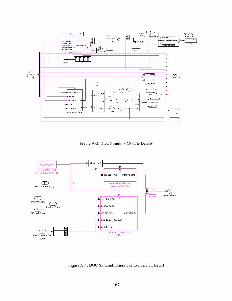
Figure A-3: DOC Simulink Module Details
Figure A-4: DOC Simulink Emissions Conversion Detail
167

Figure A-5: DOC Simulink Emissions Conversion Detail (Each Species)
Figure A-6: DOC Simulink Pressure Drop Model
168

Figure A-7: DOC Simulink Exhaust Gas Heat Flow Details
Figure A-8: DOC Simulink Exhaust System Heat Flow Details
169
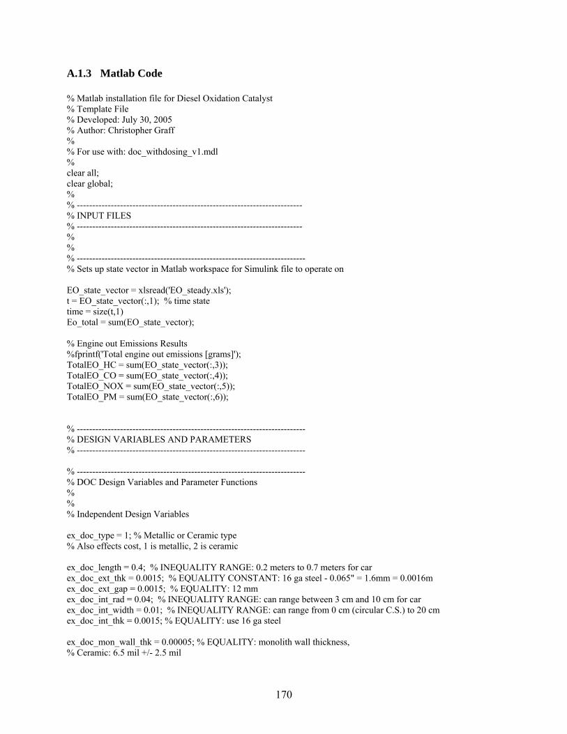
A.1.3 Matlab Code % Matlab installation file for Diesel Oxidation Catalyst % Template File % Developed: July 30, 2005 % Author: Christopher Graff % % For use with: doc_withdosing_v1.mdl % clear all; clear global; % % ------------------------------------------------------------------------- % INPUT FILES % ------------------------------------------------------------------------- % % % -------------------------------------------------------------------------- % Sets up state vector in Matlab workspace for Simulink file to operate on EO_state_vector = xlsread('EO_steady.xls'); t = EO_state_vector(:,1); % time state time = size(t,1) Eo_total = sum(EO_state_vector); % Engine out Emissions Results %fprintf('Total engine out emissions [grams]'); TotalEO_HC = sum(EO_state_vector(:,3)); TotalEO_CO = sum(EO_state_vector(:,4)); TotalEO_NOX = sum(EO_state_vector(:,5)); TotalEO_PM = sum(EO_state_vector(:,6)); % -------------------------------------------------------------------------- % DESIGN VARIABLES AND PARAMETERS % -------------------------------------------------------------------------- % -------------------------------------------------------------------------- % DOC Design Variables and Parameter Functions % % % Independent Design Variables ex_doc_type = 1; % Metallic or Ceramic type % Also effects cost, 1 is metallic, 2 is ceramic ex_doc_length = 0.4; % INEQUALITY RANGE: 0.2 meters to 0.7 meters for car ex_doc_ext_thk = 0.0015; % EQUALITY CONSTANT: 16 ga steel - 0.065" = 1.6mm = 0.0016m ex_doc_ext_gap = 0.0015; % EQUALITY: 12 mm ex_doc_int_rad = 0.04; % INEQUALITY RANGE: can range between 3 cm and 10 cm for car ex_doc_int_width = 0.01; % INEQUALITY RANGE: can range from 0 cm (circular C.S.) to 20 cm ex_doc_int_thk = 0.0015; % EQUALITY: use 16 ga steel ex_doc_mon_wall_thk = 0.00005; % EQUALITY: monolith wall thickness, % Ceramic: 6.5 mil +/- 2.5 mil
170
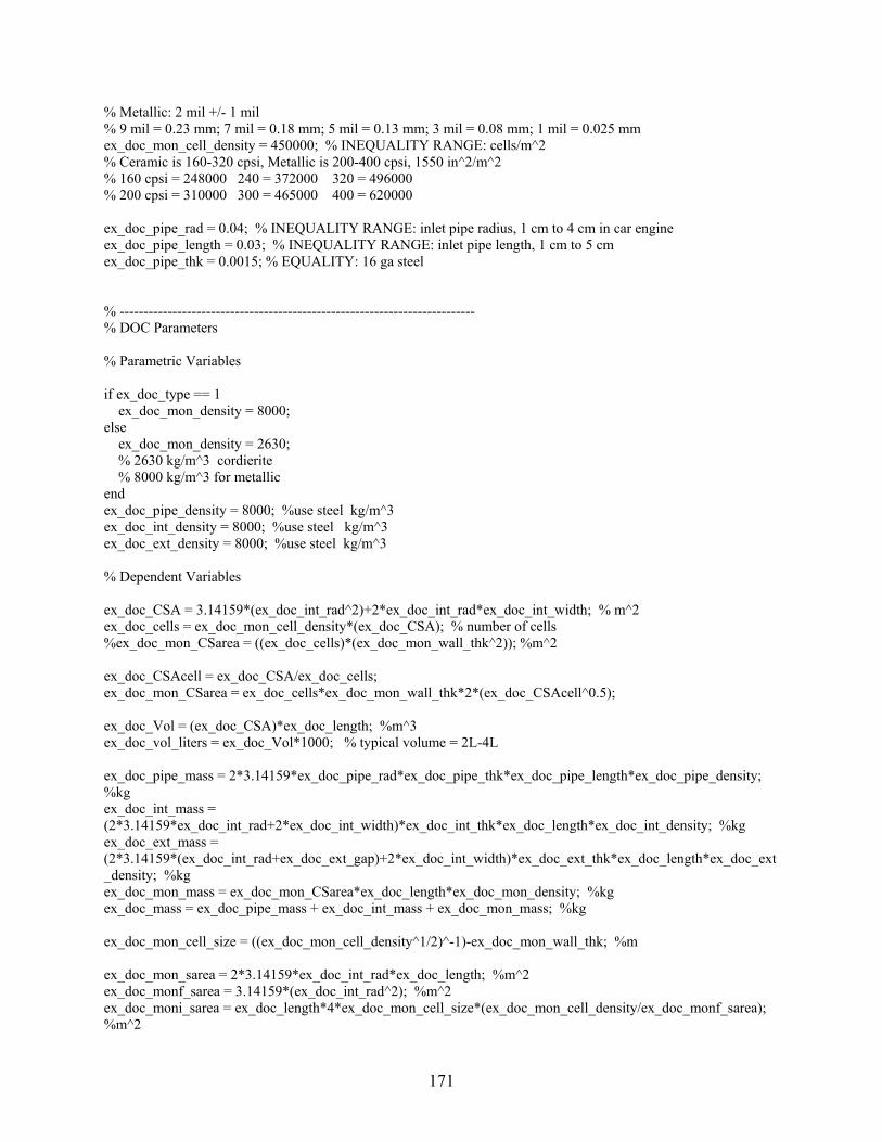
% Metallic: 2 mil +/- 1 mil % 9 mil = 0.23 mm; 7 mil = 0.18 mm; 5 mil = 0.13 mm; 3 mil = 0.08 mm; 1 mil = 0.025 mm ex_doc_mon_cell_density = 450000; % INEQUALITY RANGE: cells/m^2 % Ceramic is 160-320 cpsi, Metallic is 200-400 cpsi, 1550 in^2/m^2 % 160 cpsi = 248000 240 = 372000 320 = 496000 % 200 cpsi = 310000 300 = 465000 400 = 620000 ex_doc_pipe_rad = 0.04; % INEQUALITY RANGE: inlet pipe radius, 1 cm to 4 cm in car engine ex_doc_pipe_length = 0.03; % INEQUALITY RANGE: inlet pipe length, 1 cm to 5 cm ex_doc_pipe_thk = 0.0015; % EQUALITY: 16 ga steel % -------------------------------------------------------------------------- % DOC Parameters % Parametric Variables if ex_doc_type == 1 ex_doc_mon_density = 8000; else ex_doc_mon_density = 2630; % 2630 kg/m^3 cordierite % 8000 kg/m^3 for metallic end ex_doc_pipe_density = 8000; %use steel kg/m^3 ex_doc_int_density = 8000; %use steel kg/m^3 ex_doc_ext_density = 8000; %use steel kg/m^3 % Dependent Variables ex_doc_CSA = 3.14159*(ex_doc_int_rad^2)+2*ex_doc_int_rad*ex_doc_int_width; % m^2 ex_doc_cells = ex_doc_mon_cell_density*(ex_doc_CSA); % number of cells %ex_doc_mon_CSarea = ((ex_doc_cells)*(ex_doc_mon_wall_thk^2)); %m^2 ex_doc_CSAcell = ex_doc_CSA/ex_doc_cells; ex_doc_mon_CSarea = ex_doc_cells*ex_doc_mon_wall_thk*2*(ex_doc_CSAcell^0.5); ex_doc_Vol = (ex_doc_CSA)*ex_doc_length; %m^3 ex_doc_vol_liters = ex_doc_Vol*1000; % typical volume = 2L-4L ex_doc_pipe_mass = 2*3.14159*ex_doc_pipe_rad*ex_doc_pipe_thk*ex_doc_pipe_length*ex_doc_pipe_density; %kg ex_doc_int_mass = (2*3.14159*ex_doc_int_rad+2*ex_doc_int_width)*ex_doc_int_thk*ex_doc_length*ex_doc_int_density; %kg ex_doc_ext_mass = (2*3.14159*(ex_doc_int_rad+ex_doc_ext_gap)+2*ex_doc_int_width)*ex_doc_ext_thk*ex_doc_length*ex_doc_ext_density; %kg ex_doc_mon_mass = ex_doc_mon_CSarea*ex_doc_length*ex_doc_mon_density; %kg ex_doc_mass = ex_doc_pipe_mass + ex_doc_int_mass + ex_doc_mon_mass; %kg ex_doc_mon_cell_size = ((ex_doc_mon_cell_density^1/2)^-1)-ex_doc_mon_wall_thk; %m ex_doc_mon_sarea = 2*3.14159*ex_doc_int_rad*ex_doc_length; %m^2 ex_doc_monf_sarea = 3.14159*(ex_doc_int_rad^2); %m^2 ex_doc_moni_sarea = ex_doc_length*4*ex_doc_mon_cell_size*(ex_doc_mon_cell_density/ex_doc_monf_sarea); %m^2
171
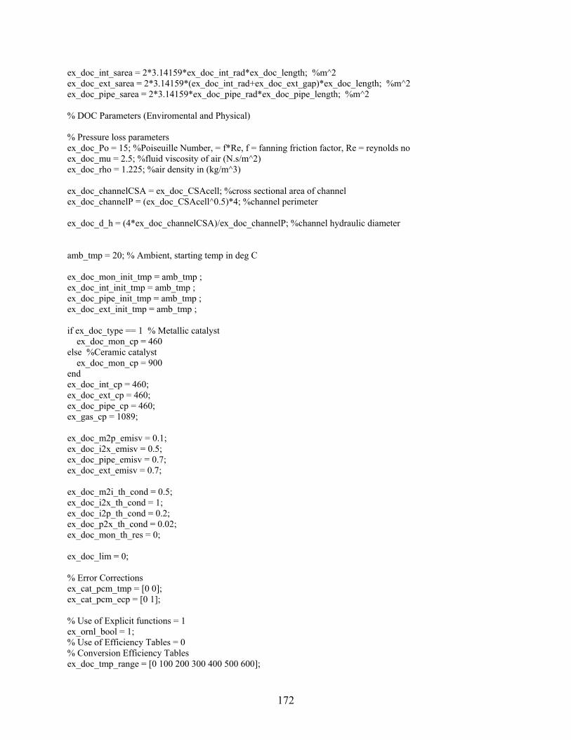
ex_doc_int_sarea = 2*3.14159*ex_doc_int_rad*ex_doc_length; %m^2 ex_doc_ext_sarea = 2*3.14159*(ex_doc_int_rad+ex_doc_ext_gap)*ex_doc_length; %m^2 ex_doc_pipe_sarea = 2*3.14159*ex_doc_pipe_rad*ex_doc_pipe_length; %m^2 % DOC Parameters (Enviromental and Physical) % Pressure loss parameters ex_doc_Po = 15; %Poiseuille Number, = f*Re, f = fanning friction factor, Re = reynolds no ex_doc_mu = 2.5; %fluid viscosity of air (N.s/m^2) ex_doc_rho = 1.225; %air density in (kg/m^3) ex_doc_channelCSA = ex_doc_CSAcell; %cross sectional area of channel ex_doc_channelP = (ex_doc_CSAcell^0.5)*4; %channel perimeter ex_doc_d_h = (4*ex_doc_channelCSA)/ex_doc_channelP; %channel hydraulic diameter amb_tmp = 20; % Ambient, starting temp in deg C ex_doc_mon_init_tmp = amb_tmp ; ex_doc_int_init_tmp = amb_tmp ; ex_doc_pipe_init_tmp = amb_tmp ; ex_doc_ext_init_tmp = amb_tmp ; if ex_doc_type == 1 % Metallic catalyst ex_doc_mon_cp = 460 else %Ceramic catalyst ex_doc_mon_cp = 900 end ex_doc_int_cp = 460; ex_doc_ext_cp = 460; ex_doc_pipe_cp = 460; ex_gas_cp = 1089; ex_doc_m2p_emisv = 0.1; ex_doc_i2x_emisv = 0.5; ex_doc_pipe_emisv = 0.7; ex_doc_ext_emisv = 0.7; ex_doc_m2i_th_cond = 0.5; ex_doc_i2x_th_cond = 1; ex_doc_i2p_th_cond = 0.2; ex_doc_p2x_th_cond = 0.02; ex_doc_mon_th_res = 0; ex_doc_lim = 0; % Error Corrections ex_cat_pcm_tmp = [0 0]; ex_cat_pcm_ecp = [0 1]; % Use of Explicit functions = 1 ex_ornl_bool = 1; % Use of Efficiency Tables = 0 % Conversion Efficiency Tables ex_doc_tmp_range = [0 100 200 300 400 500 600];
172
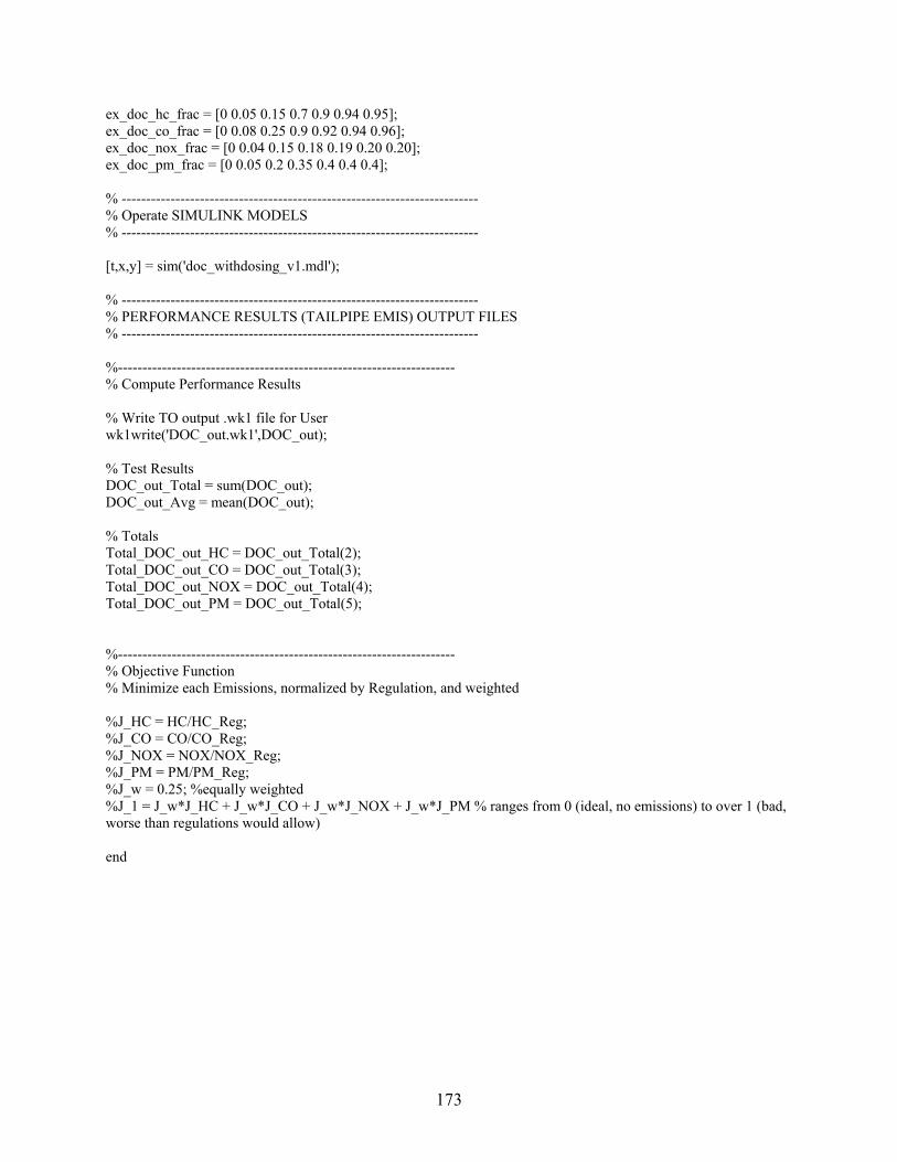
ex_doc_hc_frac = [0 0.05 0.15 0.7 0.9 0.94 0.95]; ex_doc_co_frac = [0 0.08 0.25 0.9 0.92 0.94 0.96]; ex_doc_nox_frac = [0 0.04 0.15 0.18 0.19 0.20 0.20]; ex_doc_pm_frac = [0 0.05 0.2 0.35 0.4 0.4 0.4]; % ------------------------------------------------------------------------- % Operate SIMULINK MODELS % ------------------------------------------------------------------------- [t,x,y] = sim('doc_withdosing_v1.mdl'); % ------------------------------------------------------------------------- % PERFORMANCE RESULTS (TAILPIPE EMIS) OUTPUT FILES % ------------------------------------------------------------------------- %--------------------------------------------------------------------- % Compute Performance Results % Write TO output .wk1 file for User wk1write('DOC_out.wk1',DOC_out); % Test Results DOC_out_Total = sum(DOC_out); DOC_out_Avg = mean(DOC_out); % Totals Total_DOC_out_HC = DOC_out_Total(2); Total_DOC_out_CO = DOC_out_Total(3); Total_DOC_out_NOX = DOC_out_Total(4); Total_DOC_out_PM = DOC_out_Total(5); %--------------------------------------------------------------------- % Objective Function % Minimize each Emissions, normalized by Regulation, and weighted %J_HC = HC/HC_Reg; %J_CO = CO/CO_Reg; %J_NOX = NOX/NOX_Reg; %J_PM = PM/PM_Reg; %J_w = 0.25; %equally weighted %J_1 = J_w*J_HC + J_w*J_CO + J_w*J_NOX + J_w*J_PM % ranges from 0 (ideal, no emissions) to over 1 (bad, worse than regulations would allow) end
173
A.2 Diesel Particulate Filter (DPF)
A.2.1 Assumptions, Basis Model, and Equations The model developed to describe the behavior a DPF during the loading and regeneration process is based on a 0-D, lumped parameter analysis that included a filtration model [9, 10, 16, 17, 20, 24, 25, 26, 31, 33, 42, 44]. The model assumes that the total volume of the filter is the control volume, and that the only spatial variance is the distribution of the particulate mass through the filter’s walls. The major assumptions are as follows:
• The filtration model used for calculating the filter collection efficiency treats the ceramic walls as a packed bed of uniform spherical collectors. Brownian diffusion and direct interception are assumed to be the two dominant collection mechanisms.
• The pressure drop through the filter is modeled using fluid dynamic flow through channels using the physical properties of the monolith, in addition to temperature and collected particulate mass effects.
• The particulate mass collected in the filter is distributed evenly radially and axially through the filter, and is only spatially described through the thickness of the wall.
• The temperature of the filter does not have a spatial variation, but it does vary between the major components of the filter (e.g. insulation, monolith, exterior shell, etc.)
A.2.2 Filtration Model The filtration model is divided into two regimes, the particulate that’s collected within the filter wall, and the particulate that collects on the surface of the filter wall. Within the wall, the model discretizes the filter wall along its thickness into slabs. And then within each slab, the microstructure of the model is based on a “unit collection” mechanism, with Brownian and direct interception models for the collection efficiency.
174

Figure A-9: DPF Wall Slab Filtration Diagram
For each slap, the “unit collector” filtration theory is applied locally. This unit collector model is used to describe the microstructure of the porous wall. As particulates are passed through the porous layer, they are deposited in the unit collector until it fills its space. The amount of particulates that can be stored depends on the ratio between the free volume and the collector volume. Also, the efficiency of the filtration depends on this ratio (as large amounts of free volume will allow more particulates through). Unit collector microstructure model within each slab is illustrated in Figure A-10.
Figure A-10: DPF Unit Collector Diagram
inm&
inmE &1
inmEm && )1( 12 −=
inm&
ii mE &
iiout mEm && )1( −=
x1 1
x2
2 x3
3 x4
4
xi i
xi+1
Particulates
Unit Cell Unit Collectors
175
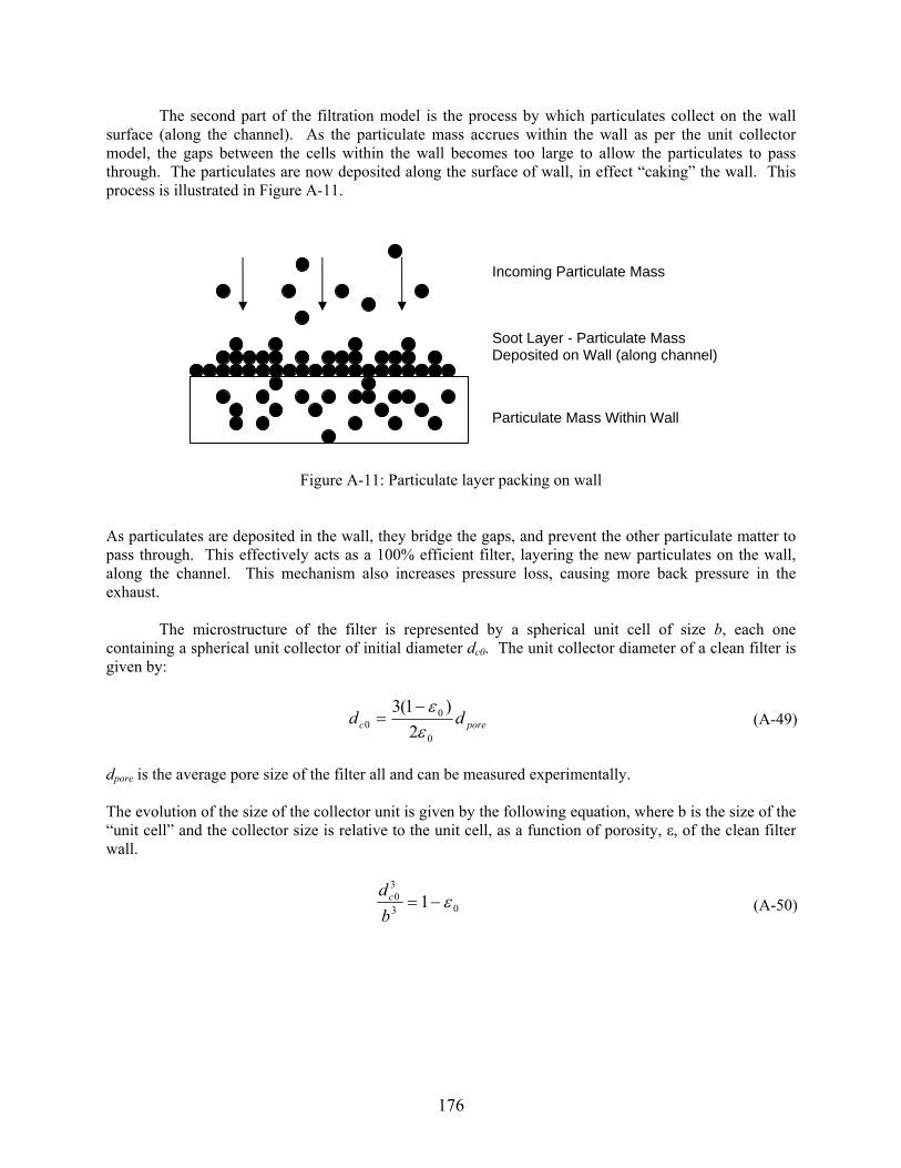
The second part of the filtration model is the process by which particulates collect on the wall surface (along the channel). As the particulate mass accrues within the wall as per the unit collector model, the gaps between the cells within the wall becomes too large to allow the particulates to pass through. The particulates are now deposited along the surface of wall, in effect “caking” the wall. This process is illustrated in Figure A-11.
Incoming Particulate Mass
Soot Layer - Particulate Mass Deposited on Wall (along channel)
Particulate Mass Within Wall
Figure A-11: Particulate layer packing on wall
As particulates are deposited in the wall, they bridge the gaps, and prevent the other particulate matter to pass through. This effectively acts as a 100% efficient filter, layering the new particulates on the wall, along the channel. This mechanism also increases pressure loss, causing more back pressure in the exhaust.
The microstructure of the filter is represented by a spherical unit cell of size b, each one
containing a spherical unit collector of initial diameter dc0. The unit collector diameter of a clean filter is given by:
pored0
0
2)1(3
εcd 0ε−
= (A-49)
dpore is the average pore size of the filter all and can be measured experimentally. The evolution of the size of the collector unit is given by the following equation, where b is the size of the “unit cell” and the collector size is relative to the unit cell, as a function of porosity, ε, of the clean filter wall.
01 ε−=3
30
bdc
(A-50)
176
A.2.3 Brownian and Direct Interception Collection Mechanisms The particle collection mechanism is assumed to be a combination of Brownian diffusion and direct intercept mechanism.
(A-51) RDRDDR ηηηηη ⋅−+=
Direct interception method collection efficiency is defined by a function of the Peclet number and a geometric parameter, g(ε), by Kuwabara [24].
(A-52) 3/2)(5.3 −⋅⋅= Peg εDη
The Peclet number is defined by the interstitial or pore velocity, Ui, the diameter of the unit collector, dc, and the Diffusion coefficient, D.
DdU ci=Pe (A-53)
The interstitial velocity is defined by the approach velocity uw, and the porosity, ε.
εwu
=iU
(A-54)
The Diffusion coefficient, D, is a function of Boltzman’s constant, kB, temperature, dynamic viscosity, the particulate diameter, and the Stokes-Cunningham slip correction factor, which accounts for transitional and slip flow effects at the unit collector surface.
SCFdTk
p
B
πµ3D =
SCF
(A-55)
The Stokes-Cunningham Slip correction factor is defined by the particle Knudsen number.
(A-56) )4.0257.1(1 /1.1 pKnp eKn −++=
The Knudsen number is defined by the particulate diameter and the mean free path of the exhaust gas.
pp d
Kn λ2= (A-57)
177
The mean free path of the exhaust gas is defined as a function of exhaust kinematic viscosity, molecular weight of the exhaust gas, temperature and the gas constant.
RTMWv
2πλ =
(A-58)
The Kuwabara geometric function for the unit cell model is defined as a function of the porosity, as it evolves over time.
3/1
23/1 )1(51)1(
592
)⎟⎟⎟⎟
⎠
⎞
⎜⎜⎜⎜
⎝
⎛
−−−−−=
εεε
ε(εg (A-59)
The Interception Collection efficiency is defined as a function of the interception parameter, and the Kuwabara geometric function.
εε
ε
323
32
)1(
))((5.1 −
+⋅=
R
R
N
gNηR (A-60)
Where the direct interception parameter is a function of the particulate diameter and the collector diameter.
c
p
dd
=RN (A-61)
The total collection efficiency, E, for the clean filter wall can be related to the single unit collector filtration efficiency by integrating a cross the filter all thickness, w, and given by the following.
⎟⎟⎠
⎞⎜⎜⎝
⎛ −−
−= 00
0
2)1(3
1 c
DR
dw
e εεη
E (A-62)
We now need to develop the collection efficiency equation for each slab of the filter cross section as it evolves in time. The evolution of the unit collector diameter is mainly a function of the mass of soot it collects over time.
3/130
, 2),(
432), ⎟
⎟⎠
⎞⎜⎜⎝
⎛⎟⎠⎞
⎜⎝⎛+= c
wsoot
w dtimt
ρπ(c id
(A-63)
178

ρsoot,w is the particulate packing density inside the filter wall. This variable needs to be defined experimentally, or sourced from different references. The porosity then changes at each slab, as a function of the varying collector diameter
( )0
3
0
1),(
1) ε−⎟⎟⎠
⎞⎜⎜⎝
⎛−=
c
c
dtid
t,(ε i (A-64)
The local permeability, k, at each slab also changes with time as particulate mass is deposited along the filter all. This can be related to the permeability the clean filter, k0, as by:
)()),((),()
0
2
0 εεf
tifd
tidt
c
c⎟⎟⎠
⎞⎜⎜⎝
⎛=
,(
0kik (A-65)
Where f(ε) is another geometric Kuwabara function for the unit cell model.
)1(
)1(51)1(
592
92)
23/1
ε
εεε
−
⎟⎠⎞
⎜⎝⎛ −−−−−
=(εf (A-66)
The local collection efficiency at each slab can be calculated from the quantities already known:
⎟⎟⎠
⎞⎜⎜⎝
⎛ −−− +
−= ),(),(2)))(,(1)(,(3 1
1), tidtixxtiti
c
iiDR
et εεη
(iE (A-67)
where x is the filter wall thickness. The above theory applies to the particulate mass collected inside the filter wall, which is also called the “deep bed” filtration regime. The additional mass collected as the particulate mass layer on the surface of the filter wall, the so called “cake” filtration regime. The partition coefficient, ψ, determines the fraction of the inlet mass that will be deposited as the particulate layer on the surface of the filter wall and is assumed to be given by the following:
20
2
20
2
)()),1((
)c
cc
dbdtd
−⋅
−=
ψ(tΦ (A-68)
From this, we develop the model for collection of particulate mass on the filter walls.
179
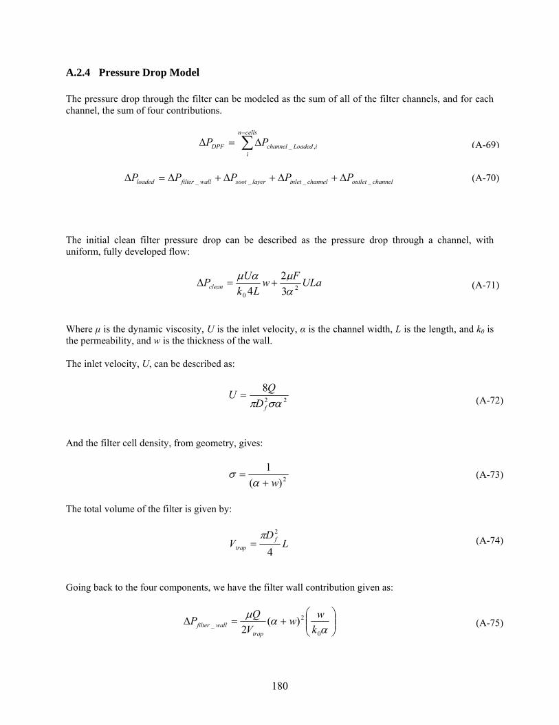
A.2.4 Pressure Drop Model The pressure drop through the filter can be modeled as the sum of all of the filter channels, and for each channel, the sum of four contributions.
∑−
∆=cellsn
iiLoadedchannelDPF P ,_∆P
P
(A-69)
(A-70) channeloutletchannelinletlayersootwallfilterloaded PPPP ____ ∆+∆+∆+∆=∆
The initial clean filter pressure drop can be described as the pressure drop through a channel, with uniform, fully developed flow:
ULaFwLk
Uclean 2
0 32
4 αP µαµ
+=∆ (A-71)
Where µ is the dynamic viscosity, U is the inlet velocity, α is the channel width, L is the length, and k0 is the permeability, and w is the thickness of the wall. The inlet velocity, U, can be described as:
22
8σαπ fDQU = (A-72)
And the filter cell density, from geometry, gives:
2)(1
w+α=σ (A-73)
The total volume of the filter is given by:
LD f
4
2π=Vtrap (A-74)
Going back to the four components, we have the filter wall contribution given as:
⎟⎟⎠
⎞⎜⎜⎝
⎛+=
ααµ
0
2_ )(
2 kww
VQ
trapwallfilter∆P (A-75)
180

And the soot layer contribution given as:
⎟⎟⎠
⎞⎜⎜⎝
⎛−
+=ssootf
layersoot ww
kDLQ
2ln)( 2
2_ ααα
πµ
∆P (A-76)
The volume of the soot on the surface of the channel changes, as per the geometry of the channel and the thickness of the soot layer
csootcells
c
Nm
,ρ=sootV (A-77)
α is the cell width, L is the cell length, ws is the thickness of the soot layer
Lww
ss
2)2(
4Vsoot−+
=αα
(A-78)
Resolved for the thickness of the soot layer
2,
2
csootcells
c
LNm
ραα −−
=sw (A-79)
where ρsoot,c is the particulate packing density. Modifying the initial equation to account for the decrease in opening of the inlet loaded channel, the inlet velocity now becomes:
22 )2(8
sf wDQ−ασπ
U = (A-80)
And now this can be substituted within the pressure components for the inlet and outlet channels
(A-81) ⎟⎟⎠
⎞⎜⎜⎝
⎛−
+= 2
22
_ )2(34)(
2 strapchannelinlet w
FLwV
Qα
αµ∆P
⎟⎟⎠
⎞⎜⎜⎝
⎛+= 4
22
_ 34)(
2 ααµ FLw
VQ
trapchanneloutlet∆P (A-82)
181
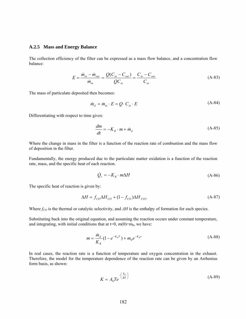
A.2.5 Mass and Energy Balance The collection efficiency of the filter can be expressed as a mass flow balance, and a concentration flow balance:
in
outin
in
outin
in
outin
CCC
QCCCQ
mmm
E−
=−
=− )(&
&&=
md
(A-83)
The mass of particulate deposited then becomes:
(A-84) ECQEm inin ⋅⋅=⋅= && Differentiating with respect to time gives:
dR mmK &+⋅−=dtdm
Qr&
H
(A-85)
Where the change in mass in the filter is a function of the reaction rate of combustion and the mass flow of deposition in the filter. Fundamentally, the energy produced due to the particulate matter oxidation is a function of the reaction rate, mass, and the specific heat of each reaction.
(A-86) HmK R ∆⋅−= The specific heat of reaction is given by:
(A-87) 2)1( COCOCOCO HfHf ∆−+∆=∆ Where fCO is the thermal or catalytic selectivity, and ∆H is the enthalpy of formation for each species. Substituting back into the original equation, and assuming the reaction occurs under constant temperature, and integrating, with initial conditions that at t=0, m(0)=m0, we have:
rKTK
R
d RR emeKm −− +− 0)1(&
m = (A-88)
In real cases, the reaction rate is a function of temperature and oxygen concentration in the exhaust. Therefore, the model for the temperature dependence of the reaction rate can be given by an Arrhenius form basis, as shown:
⎟⎠
⎞⎜⎝
⎛−RTE
TeA0
0=K (A-89)
182
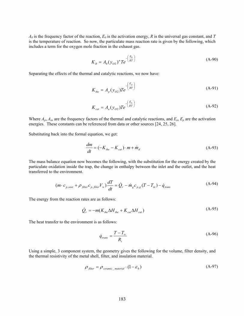
A0 is the frequency factor of the reaction, E0 is the activation energy, R is the universal gas constant, and T is the temperature of reaction. So now, the particulate mass reaction rate is given by the following, which includes a term for the oxygen mole fraction in the exhaust gas.
⎟⎠
⎞⎜⎝
⎛−
= RTE
nO TeyA
0
)( 20RK (A-90)
Separating the effects of the thermal and catalytic reactions, we now have:
⎟⎟⎠
⎞⎜⎜⎝
⎛−
= RTE
Op
p
TeyA )( 2theK (A-91)
⎟⎠
⎞⎜⎝
⎛−
= RTE
Oa
a
TeyA )( 2catK (A-92)
Where Ap, Aa, are the frequency factors of the thermal and catalytic reactions, and Ea, Ep are the activation energies. These constants can be referenced from data or other sources [24, 25, 26]. Substituting back into the formal equation, we get:
dcatthe mmKK &+⋅−−= )( dtdm
The mass balance equation now becomes the following, with the substitution for the energy created by the particulate oxidation inside the trap, the change in enthalpy between the inlet and the outlet, and the heat transferred to the environment.
(A-93)
transingpgrwfilterpfiltersootp qTTcmQdtdTVcc &&& −−−=+ )() ,,, ρm ⋅(
rQ&
(A-94)
The energy from the reaction rates are as follows:
(A-95) )( catcatthethe HKHKm ∆+∆−= The heat transfer to the environment is as follows:
tRTT ∞−
=transq& (A-96)
Using a simple, 3 component system, the geometry gives the following for the volume, filter density, and the thermal resistivity of the metal shell, filter, and insulation material.
(A-97) )1( 0_ ερρ −⋅= materialceramicfilter
183

(A-98) channelstrap VVwV −=
hLrkrr
Lkrr
shellshell
insshell
ins
filterins
πππ 21
2)/ln(
2)/ln(
++=Rt (A-99)
A.2.6 Simulink Implementation
Figure A-12: DPF Simulink Module
184
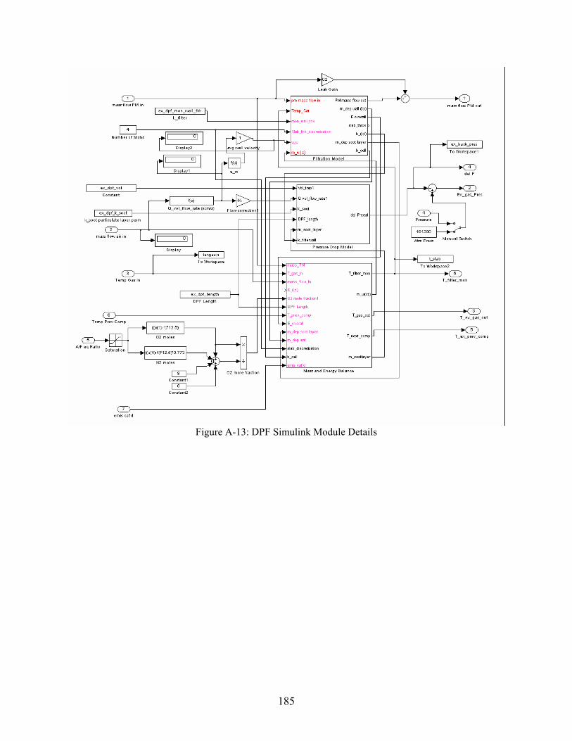
Figure A-13: DPF Simulink Module Details
185

Figure A-14: DPF Simulink Wall Filtration Details
Figure A-15: DPF Simulink Wall Filtration Percolation Details
186

Figure A-16: DPF Simulink Slab Filtration Details
Figure A-17: DPF Simulink Soot Layer Details
187
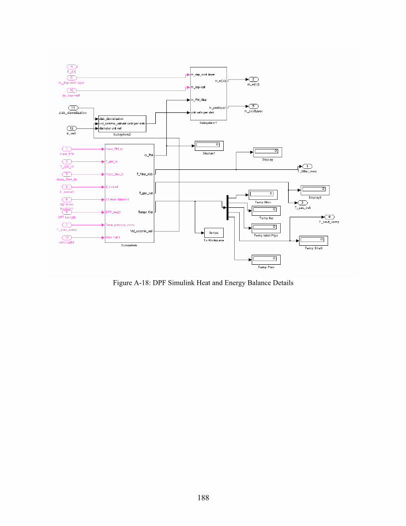
Figure A-18: DPF Simulink Heat and Energy Balance Details
188

Figure A-19: DPF Simulink Collected PM Details
189

Figure A-20: DPF Simulink PM Regeneration Details
A.2.7 Matlab Code % Matlab installation file for Diesel Exhaust System Set-up % Template File % Developed: July 30, 2005 % Author: Christopher Graff % clear all; clear global; % ------------------------------------------------------------------------- % INPUT FILES % ------------------------------------------------------------------------- % -------------------------------------------------------------------------- % Sets up state vector in Matlab workspace for Simulink file to operate on
190

EO_state_vector = xlsread('EO_steady_90mins_dirty2.xls'); t = EO_state_vector(:,1); % time state time = size(t,1) Eo_total = sum(EO_state_vector); % Emissions Results from Engine Output File fprintf('Total engine out emissions [grams]'); TotalEO_HC = sum(EO_state_vector(:,3)); TotalEO_CO = sum(EO_state_vector(:,4)); TotalEO_NOX = sum(EO_state_vector(:,5)); TotalEO_PM = sum(EO_state_vector(:,6)); % -------------------------------------------------------------------------- % DESIGN VARIABLES AND PARAMETERS % -------------------------------------------------------------------------- % -------------------------------------------------------------------------- % DPF Sizing Design Variables ex_dpf_length = 0.3; % INEQUALITY RANGE: 0.2 meters to 0.7 meters ex_dpf_shell_rad = 0.13; % INEQUALITY RANGE: can range between 3 cm and 10 cm ex_dpf_shell_width = 0.00; % INEQUALITY RANGE: can range from 0 cm (circular C.S.) to 20 cm ex_dpf_shell_thk = 0.0015; % EQUALITY: use 16 ga steel ex_dpf_insulation_thk = 0.01; ex_dpf_mon_wall_thk = 0.0005; % EQUALITY: monolith wall thickness, 0.5mm % Typical = 17 mil = 17/1000" or 0.432mm ex_dpf_mon_cell_density = 155000; % INEQUALITY RANGE: cells/m^2 MEtallic is 160-320 cpsi, Ceramic is 200-400 cpsi, 1550 in^2/m^2 % Typical = 100 CPSI % 100 cpsi = 155000 % 200 cpsi = 310000 ex_dpf_inletpipe_rad = 0.05; % INEQUALITY RANGE: inlet pipe radius, 1 cm to ? ex_dpf_inletpipe_length = 0.03; % INEQUALITY RANGE: inlet pipe length, 1 cm to ? ex_dpf_inletpipe_thk = 0.0015; % EQUALITY: 16 ga steel % -------------------------------------------------------------------------- % DPF Purge Characteristics Variables ex_dpf_purge_threshold = 9000; % Pa (backpressure to begin purge) ex_dpf_purge_temp = 650; % Temp degC of purge (if so controlled) ex_dpf_purge_end = 6000; % Pa (backpressure to end purge) ex_dpf_purge_temp_limit = 1200; %deg C ex_dpf_amb_temp = 20; %ambient air temp in deg C % -------------------------------------------------------------------------- % Parameters (Design, Enviromental/Physical) ex_dpf_diesel_stoich = 14.5; % Diesel Stoich A/F ratio (Constant) ex_dpf_density_air_conversion = .700; %kg/m^3 ---- g/s to /s conversion - constant for Q (Same in Advisor) % Densities ex_dpf_mon_density = 2630; %kg/m^3 cordierite ex_dpf_inletpipe_density = 8000; %use steel kg/m^3 ex_dpf_shell_density = 8000; %use steel kg/m^3
191
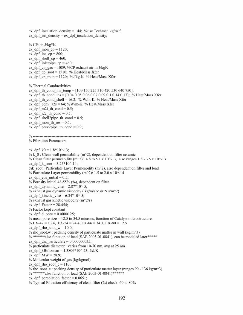
ex_dpf_insulation_density = 144; %use Techmat kg/m^3 ex_dpf_ins_density = ex_dpf_insulation_density; % CPs in J/kg*K ex_dpf_mon_cp = 1120; ex_dpf_ins_cp = 800; ex_dpf_shell_cp = 460; ex_dpf_inletpipe_cp = 460; ex_dpf_cp_gas = 1089; %CP exhaust air in J/kgK ex_dpf_cp_soot = 1510; % Heat/Mass Xfer ex_dpf_cp_mon = 1120; %J/kg-K % Heat/Mass Xfer % Thermal Conductivities ex_dpf_th_cond_ins_temp = [100 150 225 310 420 530 640 750]; ex_dpf_th_cond_ins = [0.04 0.05 0.06 0.07 0.09 0.1 0.14 0.17]; % Heat/Mass Xfer ex_dpf_th_cond_shell = 16.2; % W/m-K % Heat/Mass Xfer ex_dpf_conv_a2s = 64; %W/m-K % Heat/Mass Xfer ex_dpf_m2i_th_cond = 0.5; ex_dpf_i2c_th_cond = 0.5; ex_dpf_shell2pipe_th_cond = 0.5; ex_dpf_mon_th_res = 0.5; ex_dpf_prev2pipe_th_cond = 0.9; % -------------------------------------------------------------------------- % Filtration Parameters ex_dpf_k0 = 1.8*10^-13; % k_0 : Clean wall permiability (m^2), dependent on filter ceramic % Clean filter permeability (m^2): 4.8 to 5.1 x 10^-13, also ranges 1.8 - 3.5 x 10^-13 ex_dpf_k_soot = 3.25*10^-14; %k_soot : Particulate Layer Permeability (m^2), also dependent on filter and load % Particulate Layer permeability (m^2): 1.5 to 2.0 x 10^-14 ex_dpf_eps_initial = 0.5; % Porosity initial 48-55% (%), dependent on filter ex_dpf_dynamic_visc = 2.87*10^-5; % exhaust gas dynamic viscocity ( kg/m/sec or N.s/m^2) ex_dpf_kinetic_visc = 6.34*10^-5; % exhaust gas kinetic viscocity (m^2/s) ex_dpf_Factor = 28.454; % Factor kept constant ex_dpf_d_pore = 0.0000125; % mean pore size = 12.5 to 34.5 microns, function of Catalyst microstructure % EX-47 = 13.4, EX-54 = 24.4, EX-66 = 34.1, EX-80 = 12.5 ex_dpf_rho_soot_w = 10.0; % rho_soot,w : packing density of particulate matter in wall (kg/m^3) % ******also function of load (SAE 2003-01-0841), can be modeled later***** ex_dpf_dia_particulate = 0.000000035; % particulate diameter : varies from 10-70 nm, avg at 25 nm ex_dpf_kBoltzman = 1.3806*10^-23; %J/K ex_dpf_MW = 28.9; % Molecular weight of gas (kg/kgmol) ex_dpf_rho_soot_c = 110; % rho_soot_c : packing density of particulate matter layer (ranges 90 - 136 kg/m^3) % ******also function of load (SAE 2003-01-0841)****** ex_dpf_percolation_factor = 0.8651; % Typical Filtration efficiency of clean filter (%) check: 60 to 80%
192

% -------------------------------------------------------------------------- % Heat/Energy Transfer (Oxidation Rates) ex_dpf_therm_freq_fac = 1000; % 1/K-s % Heat/Mass Xfer ex_dpf_therm_act_energy = 150000; %J/mol % Heat/Mass Xfer ex_dpf_cat_freq_fac = 450; %1/K-s % Heat/Mass Xfer ex_dpf_cat_act_energy = 120000; %J/mol % Heat/Mass Xfer ex_dpf_R = 8.314; % universal gas constant SI units ex_dpf_Cp_reaction_thermal = 3.98*10^8; %Specific heat of thermal reaction particulate oxidation 3.93x10^8 J/kgmol ex_dpf_Cp_reaction_catalytic = 3.98*10^8; %Specific heat of catalytic reaction particulate oxidation % Activation Energy (kJ/mol): thermal: 150; catalytic: 80 to 120, depending % Frequency Factor (1/K-s): thermal: 1x10^3; catalytic: 4.0-5.0 x10^2 % (cooper additive), 3.0-3.0 x10^3 (CPF) % Peclet Number check: 0.52 to 0.72 % Ambient Temperatures amb_tmp = ex_dpf_amb_temp ; ex_dpf_filter_temp_init = amb_tmp; ex_dpf_mon_init_temp = amb_tmp; ex_dpf_ins_init_temp = amb_tmp; ex_dpf_pipe_init_temp = amb_tmp; ex_dpf_shell_init_temp = amb_tmp; % Emissivities ex_dpf_m2p_emisv = 0.1; ex_dpf_inletpipe_emisv = 0.7; ex_dpf_shell_emisv = 0.7; % -------------------------------------------------------------------------- % Downpipe Parameters % %ex_dp_density = 7872; %use steel, kg/m^3 %ex_dp_pipe_cp = 460; %use steel, CP, J/kgK %ex_dp_th_cond = 1; %use steel to steel thermal conductivity % ------------------------------------------------------------------------- % Dependent Design Variables ex_dpf_ins_thk = ex_dpf_insulation_thk ; ex_dpf_insulation_rad = ex_dpf_shell_rad-ex_dpf_shell_thk; ex_dpf_ins_rad = ex_dpf_insulation_rad; ex_dpf_core_rad = ex_dpf_insulation_rad-ex_dpf_insulation_thk; ex_dpf_mon_rad = ex_dpf_core_rad; ex_dpf_channel_width = ((1/(ex_dpf_mon_cell_density))^0.5)-ex_dpf_mon_wall_thk; ex_dpf_alpha = ex_dpf_channel_width; ex_dpf_total_filtration_area = ex_dpf_channel_width*4*ex_dpf_length; ex_dpf_CSA = 3.14159*(ex_dpf_core_rad^2)+2*ex_dpf_core_rad*ex_dpf_shell_width; % m^2 ex_dpf_inlet_cells = 0.5*ex_dpf_mon_cell_density*(ex_dpf_CSA); % number of inlet cells of wall-flow filter %ex_dpf_N_cells = 0.5*(ex_dpf_mon_cell_density)*(ex_dpf_total_filtration_area); ex_dpf_mon_CSarea = (ex_dpf_inlet_cells*2*ex_dpf_mon_wall_thk*(ex_dpf_mon_wall_thk+ex_dpf_channel_width)); %m^2
193

ex_dpf_vol = ex_dpf_CSA*ex_dpf_length; %m^3 ex_dpf_vol_liters = ex_dpf_vol*1000; % ex_dpf_inletpipe_mass = 2*3.14159*ex_dpf_inletpipe_rad*ex_dpf_inletpipe_thk*ex_dpf_inletpipe_length*ex_dpf_inletpipe_density; %kg ex_dpf_ins_mass = (2*3.14159*ex_dpf_ins_rad+2*ex_dpf_shell_width)*ex_dpf_ins_thk*ex_dpf_length*ex_dpf_ins_density; %kg ex_dpf_shell_mass = (2*3.14159*(ex_dpf_shell_rad)+2*ex_dpf_shell_width)*ex_dpf_shell_thk*ex_dpf_length*ex_dpf_shell_density; %kg ex_dpf_mon_mass = ex_dpf_mon_CSarea*ex_dpf_length*ex_dpf_mon_density %kg ex_dpf_mon_sarea = 2*3.14159*ex_dpf_mon_rad*ex_dpf_length; %m^2 ex_dpf_monf_sarea = ex_dpf_mon_wall_thk*4*ex_dpf_channel_width*(ex_dpf_mon_cell_density/ex_dpf_CSA); %m^2 %ex_dpf_mon_cell_size = ((ex_dpf_mon_cell_density^1/2)^-1)-ex_dpf_mon_wall_thk; %m ex_dpf_moni_sarea = ex_dpf_length*4*ex_dpf_channel_width*(ex_dpf_mon_cell_density/ex_dpf_CSA); %m^2 ex_dpf_ins_sarea = 2*3.14159*ex_dpf_ins_rad*ex_dpf_length; %m^2 ex_dpf_shell_sarea = 2*3.14159*(ex_dpf_shell_rad)*ex_dpf_length; %m^2 ex_dpf_inletpipe_sarea = 2*3.14159*ex_dpf_inletpipe_rad*ex_dpf_inletpipe_length; %m^2 ex_dpf_mass = ex_dpf_inletpipe_mass + ex_dpf_shell_mass + ex_dpf_mon_mass + ex_dpf_ins_mass%kg % ------------------------------------------------------------------------- % Operate SIMULINK MODELS % ------------------------------------------------------------------------- [t,x,y] = sim('dpf_model_v2_1block.mdl'); % ------------------------------------------------------------------------- % PERFORMANCE RESULTS (TAILPIPE EMIS) OUTPUT FILES % ------------------------------------------------------------------------- %--------------------------------------------------------------------- % Compute Performance Results % Write TO output .wk1 file for User wk1write('DPF_Out.wk1',DPF_Out); % Test Results DPF_Out_Total = sum(DPF_Out); DPF_Out_Avg = mean(DPF_Out); End
194

A.3 Dosing System
A.3.1 Assumptions, Basis Model, Equations
The basis behind the dosing system model is that by injective fuel (or other forms of HC) over the diesel oxidation catalyst (DOC), one can utilize the reaction rates to raise the exhaust gas temperature. The simple implementation of this model is to introduce a module ahead of the DOC that basically introduces a mass flow of HC. The mass flow of HC out of this module is the sum of the incoming HC gas flow and the dosing input.
inputgdoin mm _sin&&outm& += (A-100) The model assumes droplet sizing and spray distribution will be constant and full atomization into the air flow will occur. By combining this module ahead of a DOC, the extra hydrocarbon gas flow will be able to be reacted by the DOC and raise the exhaust gas temperature [9, 17, 24]. Future advances of the dosing model can incorporate a vaporization sub-model into this module, which will track the spray pattern and atomization of the dosing input.
195

A.3.2 Simulink Implementation
A-101: Dosing System Simulink Details
196
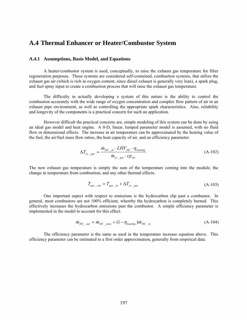
A.4 Thermal Enhancer or Heater/Combustor System
A.4.1 Assumptions, Basis Model, and Equations
A heater/combustor system is used, conceptually, to raise the exhaust gas temperature for filter regeneration purposes. These systems are considered self-contained, combustion systems, that utilize the exhaust gas air (which is rich in oxygen content, since diesel exhaust is generally very lean), a spark plug, and fuel spray input to create a combustion process that will raise the exhaust gas temperature.
The difficulty in actually developing a system of this nature is the ability to control the
combustion accurately with the wide range of oxygen concentration and complex flow pattern of air in an exhaust pipe environment, as well as controlling the appropriate spark characteristics. Also, reliability and longevity of the components is a practical concern for such an application.
However difficult the practical concerns are, simple modeling of this system can be done by using
an ideal gas model and heat engine. A 0-D, linear, lumped parameter model is assumed, with no fluid flow or dimensional effects. The increase in air temperature can be approximated by the heating value of the fuel, the air/fuel mass flow ratios, the heat capacity of air, and an efficiency parameter.
airgasex
heatingHCinHCgas cpm
LHVm⋅exT
⋅⋅=
_
__ &
&∆
η )
The new exhaust gas temperature is simply the sum of the temperature coming into the mochange in temperature from combustion, and any other thermal effects.
gasexingasout TT __gasT _ ∆+=
One important aspect with respect to emissions is the hydrocarbon slip past a combugeneral, most combustors are not 100% efficient, whereby the hydrocarbon is completely burneffectively increases the hydrocarbon emissions past the combustor. A simple efficiency paraimplemented in the model to account for this effect.
inHCheatingemisHCout mm ___ )1( &&HCm& η−+=
The efficiency parameter is the same as used in the temperature increase equation aboefficiency parameter can be estimated to a first order approximation, generally from empirical da
197
(A-102
dule, the
(A-103)
stor. In ed. This meter is
(A-104)
ve. This ta.
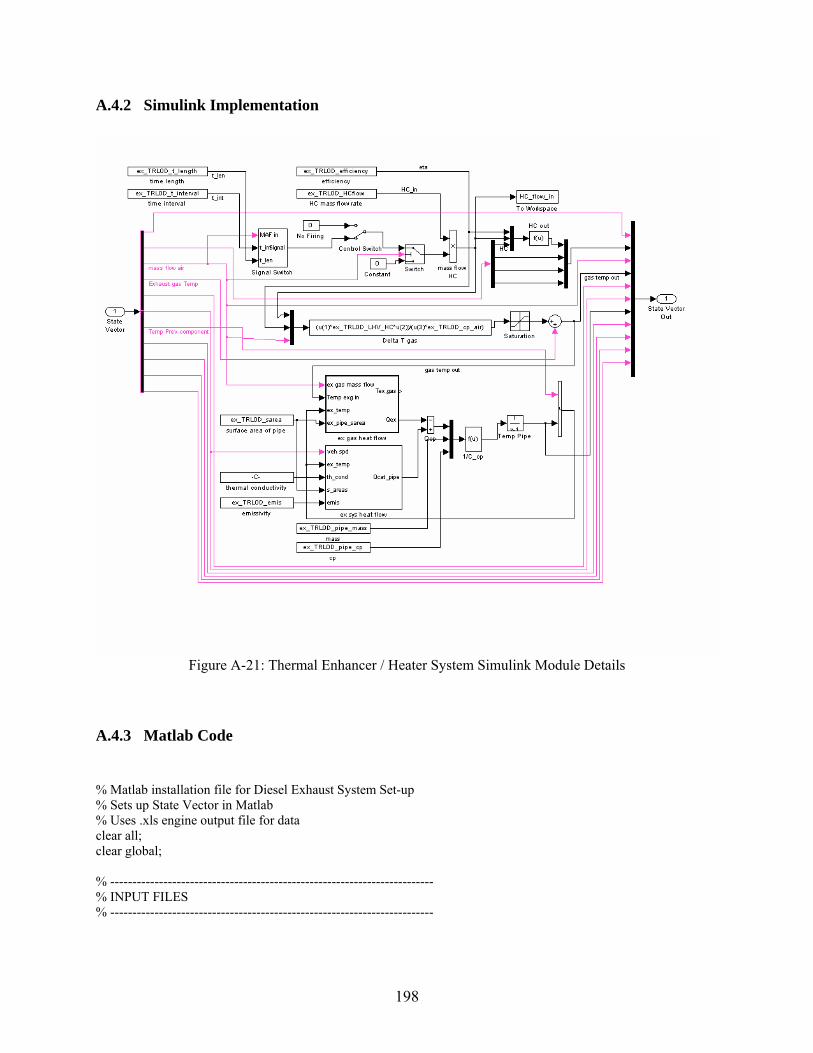
A.4.2 Simulink Implementation
Figure A-21: Thermal Enhancer / Heater System Simulink Module Details
A.4.3 Matlab Code % Matlab installation file for Diesel Exhaust System Set-up % Sets up State Vector in Matlab % Uses .xls engine output file for data clear all; clear global; % ------------------------------------------------------------------------- % INPUT FILES % -------------------------------------------------------------------------
198

% -------------------------------------------------------------------------- % Sets up state vector in Matlab workspace for Simulink file to operate on TRL_in = xlsread('EO_steady.xls'); t = TRL_in(:,1); % time state time = size(t,1) % -------------------------------------------------------------------------- % DESIGN VARIABLES AND PARAMETERS % -------------------------------------------------------------------------- % -------------------------------------------------------------------------- % DOC Design Variables and Parameter Functions % % % Independent Design Variables ex_TRL0D_length = 0.4; % INEQUALITY RANGE: 0.2 meters to 0.7 meters for car ex_TRL0D_pipe_thk = 0.0015; % EQUALITY CONSTANT: 16 ga steel - 0.065" = 1.6mm = 0.0016m ex_TRL0D_rad = 0.04; % INEQUALITY RANGE: can range between 3 cm and 10 cm for car ex_TRL0D_width = 0; %NOT USED ex_TRL0D_t_interval = 200; % seconds between intervals ex_TRL0D_t_length = 5; %length of burn ex_TRL0D_HCflow = 2; %g/s of HC in ex_TRL0D_efficiency = 0.95; %efficiency of burner % Parametric Design Variables ex_TRL0D_pipe_density = 8000; %use steel kg/m^3 ex_TRL0D_p2p_th_cond = 1; ex_TRL0D_LHV_HC = 42000 ; %kJ/kg or J/g NOT in MJ/kg ex_TRL0D_pipe_cp = 460; ex_TRL0D_cp_air = 1.006; %kJ/kg-K or J/g-K ex_TRL0D_emis = 0.7; ex_TRL0D_cp_gas = 1090; % Dependent Design Variables ex_TRL0D_sarea = 2*3.14159*ex_TRL0D_rad*ex_TRL0D_length; %kg ex_TRL0D_CSA = 3.14159*(ex_TRL0D_rad^2)+2*ex_TRL0D_rad*ex_TRL0D_width; % m^2 ex_TRL0D_Vol = (ex_TRL0D_CSA)*ex_TRL0D_length; %m^3 ex_TRL0D_vol_liters = ex_TRL0D_Vol*1000; % typical volume = 2L-4L ex_TRL0D_pipe_mass = 2*3.14159*ex_TRL0D_rad*ex_TRL0D_pipe_thk*ex_TRL0D_length*ex_TRL0D_pipe_density; %kg % Initial Temperatures amb_temp = 20; % Ambient, starting temp in deg C ex_TRL0D_init_temp = amb_temp ; % -------------------------------------------------------------------------
199
% Operate SIMULINK MODELS % ------------------------------------------------------------------------- [t,x,y] = sim('trl_0d_v1.mdl'); % ------------------------------------------------------------------------- % PERFORMANCE RESULTS (TAILPIPE EMIS) OUTPUT FILES % ------------------------------------------------------------------------- %--------------------------------------------------------------------- % Compute Performance Results % Write TO output .wk1 file for User wk1write('TRL_out.wk1',TRL_out); % Test Results Total = sum(TRL_out); Avg = mean(TRL_out); end
200

A.5 Lean NOx Trap (LNT)
A.5.1 Assumptions, Basis Model, Equations
A good understanding of the fundamental physical basis of how a NOx trap works, particularly a lean NOx trap, is reasonably well known [18, 22, 35, 38, 43]. A full one dimensional partial differential equation based description of the basic chemical and physical phenomena can be taken from prior work by Aimard et al [22]. However, a simpler, phenomenological based model can be implemented for the lean NOx trap. Lean burn engines (lean burn gasoline or diesel engines) typically utilize NOx traps to reduce emissions. When the engine is running with a lean air-fuel mixture (or rich in O2), the NO in the exhaust gas entering an LNT is catalytically oxidized to NO2. The NO2 is then stored in a nearby cell site (usually composed of alkali metal or alkaline earth material) as a nitrate (in the example below barium nitrate). During times of rich exhaust mixture, the stored NO2 is released and catalytically reduced by the reductants of CO, H2, and HC to form H20, CO2, N2, and H2.
Figure A-22: Storage and Purging of LNT (image courtesy [22])
These two phases (shown in Figure A-22) of a lean NOx trap are known as the storage and purge
phases. The mechanisms by which these processes work is complex, but can be approximated for the purposes of a system model in a phenomenological, control oriented, lumped parameter model. NOx emission levels can be controlled by properly managing the purging and storing mechanisms, via lean and richer periods, or via fuel injection in the exhaust stream. In effect, unless there is passive triggering via engine air-fuel mixture modulation, there needs to be active triggering of the LNT to purge.
The major criteria that affect the operation of the LNT are its temperature, space velocity, NOx
concentration, the availability of storage sites, and the air-fuel ratio. These variables affect the behavior of the storage capacity, storage efficiency, and NOx conversion efficiency. The model begins with a simple, mass flow of NOx in and out of the LNT.
(A-105) outNOxinNOxstored mm ,,, &&NOxm& −= The stored NOx can be described as a fraction of total LNT capacity
(A-106) xCLNTstoredmNOx ⋅=,
201

CLNT is the storage capacity (in grams or kg) and x is the fraction of capacity (or alternately, x can indicate total percent of occupied sites). Differentiating and combining the equations we get the following:
dtdxCx
dtdC
LNTLNT
stored ⋅+⋅=,mNOx& (A-107)
Storage efficiency is defined as a function of mass flow (mNOx,in) into the LNT and flow rate out of the storage sites during the storing phase (mNOx,b).
inNOx
bNOxinNOx
mmm
,
,,
&
&&s
−=η
NOxm&
(A-108)
Redefining mNOx,out, using the storage efficiency and the mass flow of NOx released during the purge phase, mNOx,r.
rNOxinNOxsrNOxbNOxout mmmm ,,,,, )1( &&&& +−=+= η (A-109) Combining the equations from above yields the following differential equation:
LNT
rNOx
LNT
inNOxs
LNT
LNT Cm
Cm
xdt
dCC
,,1 &&−⋅+− η
dtdx
=
NOxm
(A-110)
In summary, the mass flows of NOx out of the trap can be approximated by the storage efficiency during the storage phase (ηs), mass flow of NOx into the trap, mass flow released from the sites, and the conversion efficiency during the purging phase (ηc).
)1()1( ,,, creleasedNOxinNOxsout mm ηη −⋅+⋅−= &&& (A-111)
The storage dynamics of the LNT are derived from the basic chemistry of the following:
NO + ½ O2 NO2
BaCO3 + 2NO2 + ½ O2 Ba(NO3)2 + CO2 What the model does, however, is simplify the storage dynamics into two aspects, that of storage capacity and the efficiency as a function of temperatures. The storage capacity is primarily a function of trap temperature, with the maximum capacity set by geometric and catalyst formulation constraints. A typical first order approximation is shown in Figure A-23.
202
Figure A-23: NOx Storage Capacity Curve (image courtesy [22])
The capacity of the LNT is thus resolved by the following equation:
⎥⎥
⎦
⎤
⎢⎢
⎣
⎡⎟⎟⎠
⎞⎜⎜⎝
⎛ −−
⋅=
2max
wTTT
m eCLNTC (A-112)
To model the effects of temperature and capacity of LNT with its storage efficiency, or its ability to store incoming NOx mass flow, the following storage efficiency model was used:
α
αα
eee x
η s −−
1= (A-113)
α is a parameter reflecting the effect of the LNT temperature and space velocity on strage efficiency. As can be seen in the next figure, as the LNT fills the storage efficiency gradually decrease and approaches 0 when full. At any given fraction x, the storage efficiency varies with temperature and space velocity, parameter α. This parameter is modeled from empirical data, and reflects the following curve The storage efficiency is a function both of the fraction of capacity at the time, as well as temperature. A typical approximation is shown in Figure A-24.
203

Figure A-24: NOx Storage Efficiency Curves (image courtesy [22])
The storage efficiency can then be used to solve for the amount of NOx mass flow out of the trap.
The principle behind purging is to flow through rich exhaust air to the trap, where the nitrate (Ba(NO3)2 in our case) becomes unstable and releases NO2 and BaO. BaO then becomes BaCO3, and regenerates the original storage sites. The released NO2 is converted to N2 by the reductants in rich exhaust gas (CO, H2, and HC) over the precious metal sites. The purge dynamics of the NOx trap are slightly more complex, but based on chemical reactions, where first there is the regeneration of the storage sites:
Ba(NO3)2 BaO + 2NO2 + ½ O2
BaO + CO2 BaCO3
The second part is the conversion of NOx:
NO2 NO + ½ O2
NO + CO CO2 + ½ N2
9NO + C3H6 3CO2 + 3H20 + 9/2O2 The release rate of NOx is not a step process. When the exhaust gas becomes rich, the LNT
doesn’t being to release NOx immediately – there is a time delay. This delay is a function of the fact that incoming gas has to dilute the already lean air inside the LNT until all of the air is rich. Also, there is oxygen stored during the lean operating conditions within the storage sites, which also has to escape
204
during this transition period. Based on these facts, the NOx release rate can be shown to depend on the oxygen release from the oxygen storage sites, the A/F ratio of incoming air, the temperature, and the amount of NOx stored, and can be approximated by the following equation:
),,()1(11, TAFRfx
ee
Cm
OSC
x
LNT
rNOx λβ
β
−−−
=&
kr = (A-114)
xOSC is the faction of oxygen storage and beta is a parameter depending on the catalyst physical properties such as formulation, geometry, etc. xOSC captures the effect of the oxygen storage and interaction of NOx and oxygen. The oxygen storage and release mechanism is based on the Three Way Catalyst model developed by Brandt et al [22].
A look-up table can approximate the release rate as a function of A/F ratio, and LNT storage level, and can be shown to be as follows:
Figure A-25: NOx Release Rate Curves (image courtesy [22])
Note that this graphic depicts the dynamics when xOXC = 0. The A/F ratio of the exhaust gas changes as it flows through the LNT, due to the oxygen exchange to or from the oxygen storage sites. The purge process is described as:
4CeO2 2Ce2O3 + O2
205

The oxygen storage model is extended to deal with the purge process, and the A/F equivalence ratio at the outlet is described as the following
)1()1()1( −−−−−= inininout λσρλρλλ rho is the contribution of oxygen from the oxygen storage sites, and sigma is the contribution of oxygen from the NOx purge process. Sigma is calculated using the NOx release rate and the amount of air required to keep the A/F ratio at stoichiometry.
(A-115)
rNOx
inina
m
m
,
)1(1121.0
&
&
⋅
⎟⎟⎠
⎞⎜⎜⎝
⎛−−
−
ελρλ
=σ (A-116)
The second part of the release process is the conversion efficiency.
rNOx
outNOxrNOx
mmm
,
,,
&
&&c
−=η (A-117)
The efficiency depends on the air-fuel ratio, temperature, space velocity, and based on experimental data can be approximated as the following equation:
),,(1
TMAFfeee x
λγ
γγ
cη−−
= (A-118)
The conversion efficiency can be approximated by a look-up table, as shown in the following graph, which plots the conversion efficiency as a function of A/F ratio and LNT storage level.
206

Figure A-26: Conversion Efficiency Curves (image courtesy [22])
This simple model can be used as a first order approximation for the behavior of a lean NOx trap, particularly in a control oriented scenario. The application used here has distinct operational limits, and takes into account that a triggering process is needed (either active or passive) by which the exhaust gas air-fuel ratio can change and become a rich mixture to allow for the purging process to occur.
207

A.5.2 Simulink Implementation
Figure A-27: LNT Simulink Module
208
Figure A-28: LNT Simulink Module Details
Figure A-29: LNT Simulink Pressure Drop Details
209

Figure A-30: LNT Simulink Storage and Purging Code Details
210

Figure A-31: LNT Simulink NOx Capacity Details
Figure A-32: LNT Simulink Storage Efficiency Details
211
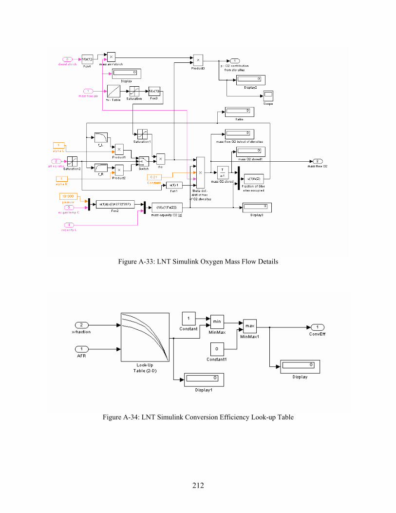
Figure A-33: LNT Simulink Oxygen Mass Flow Details
Figure A-34: LNT Simulink Conversion Efficiency Look-up Table
212
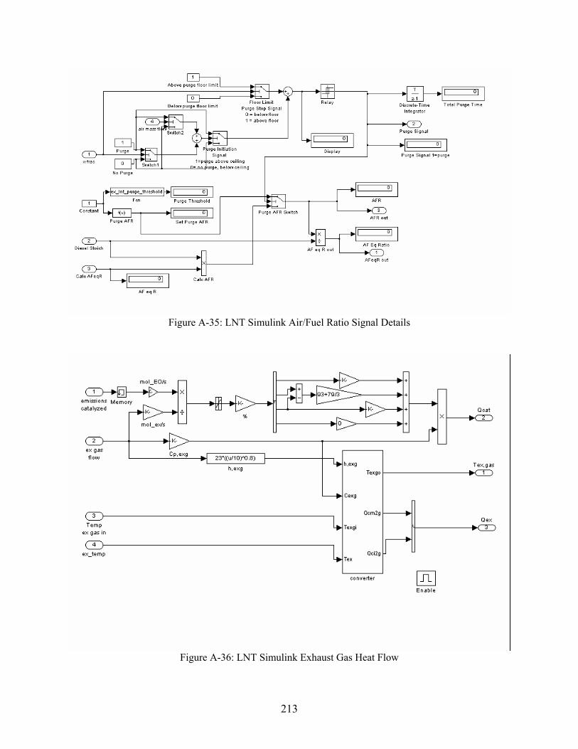
Figure A-35: LNT Simulink Air/Fuel Ratio Signal Details
Figure A-36: LNT Simulink Exhaust Gas Heat Flow
213
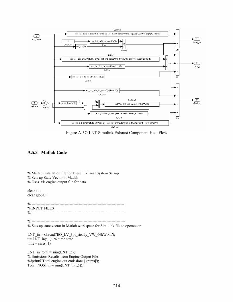
Figure A-37: LNT Simulink Exhaust Component Heat Flow
A.5.3 Matlab Code
% Matlab installation file for Diesel Exhaust System Set-up % Sets up State Vector in Matlab % Uses .xls engine output file for data clear all; clear global; % ------------------------------------------------------------------------- % INPUT FILES % ------------------------------------------------------------------------- % -------------------------------------------------------------------------- % Sets up state vector in Matlab workspace for Simulink file to operate on LNT_in = xlsread('EO_LV_3pt_steady_VW_66kW.xls'); t = LNT_in(:,1); % time state time = size(t,1) LNT_in_total = sum(LNT_in); % Emissions Results from Engine Output File %fprintf('Total engine out emissions [grams]'); Total_NOX_in = sum(LNT_in(:,5));
214

% -------------------------------------------------------------------------- % DESIGN VARIABLES AND PARAMETERS % -------------------------------------------------------------------------- % -------------------------------------------------------------------------- % Independent Design Variables % LNT Efficiency/Performance Characteristics ex_lnt_type = 1; ex_lnt_epsilon = 150000; % epsilon factor (for O2 rel/stor) purging process ex_lnt_Tm = 350; % optimal temperature ex_lnt_Ts = 80; % temperature window ex_lnt_Cm = 1.15; % g/liter of Nox capacity % LNT Sizing Variables ex_lnt_length = 0.3; ex_lnt_ext_thk = 0.0015; % 16 ga steel - 0.065" = 1.6mm = 0.0016m ex_lnt_ext_gap = 0.012; % heat shield gap ex_lnt_int_rad = 0.05; ex_lnt_int_width = 0.00; ex_lnt_int_thk = 0.0015; ex_lnt_mon_wall_thk = 0.0005; % monolith wall thickness, 0.5mm % varies between 10 and 20 mils; 10/1000" = 0.254mm ex_lnt_mon_cell_density = 310000; % cells/m^2: Ceramic is 200-400 cpsi; 1550 in^2/m^2 % 160 cpsi = 248000 240 = 372000 320 = 496000 % 200 cpsi = 310000 300 = 465000 400 = 620000 ex_lnt_pipe_rad = 0.05; % inlet pipe radius ex_lnt_pipe_length = 0.03; % inlet pipe length, 1 cm to ? ex_lnt_pipe_thk = 0.0015; % LNT Purge Characteristics ex_lnt_purge_threshold = 0.4; % Capacity of LNT full of NOx, at which LNT begins to purge ex_lnt_purge_AFR = 12.5; % Purge A/F ratio, needs to be slightly rich (11-13.5 range acceptable) ex_lnt_purge_end = 0.15; % Capacity at which LNT stops purging % See also release rate table in .mdl for details ex_lnt_release_rate_constant = 0.9; % a value used for calibration of release rate (between 0.1 and 1.5) % -------------------------------------------------------------------------- % Parameters and Dependent Variables ex_lnt_diesel_stoich = 14.5; % Diesel Stoich A/F ratio (Constant)
215

ex_lnt_CSA = 3.14159*(ex_lnt_int_rad^2)+2*ex_lnt_int_rad*ex_lnt_int_width; % m^2 ex_lnt_cells = ex_lnt_mon_cell_density*(ex_lnt_CSA); % number of cells ex_lnt_mon_CSarea = ((ex_lnt_cells)*(ex_lnt_mon_wall_thk^2)); %m^2 ex_lnt_mon_density = 2630; %kg/m^3 cordierite ex_lnt_pipe_density = 8000; %use steel kg/m^3 ex_lnt_int_density = 8000; %use steel kg/m^3 ex_lnt_ext_density = 8000; %use steel kg/m^3 % -------------------------------------------------------------------------- % Downpipe Parameters ex_dp_density = 7872; %use steel, kg/m^3 ex_dp_pipe_cp = 460; %use steel, CP, J/kgK ex_dp_th_cond = 1; %use steel to steel thermal conductivity % ------------------------------------------------------------------------- % LNT Parameters (Enviromental and Physical) % Pressure loss parameters ex_doc_Po = 15; %Poiseuille Number, = f*Re, f = fanning friction factor, Re = reynolds no ex_doc_mu = 2.5; %fluid viscosity of air (N.s/m^2) ex_doc_rho = 1.225; %air density in (kg/m^3) ex_doc_channelCSA = ex_doc_CSAcell; %cross sectional area of channel ex_doc_channelP = (ex_doc_CSAcell^0.5)*4; %channel perimeter ex_doc_d_h = (4*ex_doc_channelCSA)/ex_doc_channelP; %channel hydraulic diameter amb_tmp = 20; % Ambient, starting temp in deg C ex_lnt_mon_init_tmp = amb_tmp; ex_lnt_int_init_tmp = amb_tmp; ex_lnt_pipe_init_tmp = amb_tmp; ex_lnt_ext_init_tmp = amb_tmp; % CP in J/kg*K ex_lnt_mon_cp = 900; % cordierite ex_lnt_int_cp = 460; ex_lnt_ext_cp = 460; ex_lnt_pipe_cp = 460; ex_gas_cp = 1089; ex_lnt_m2p_emisv = 0.1; ex_lnt_i2x_emisv = 0.5; ex_lnt_pipe_emisv = 0.7; ex_lnt_ext_emisv = 0.7; ex_lnt_m2i_th_cond = 0.5; ex_lnt_i2x_th_cond = 1; ex_lnt_i2p_th_cond = 0.2; ex_lnt_p2x_th_cond = 0.02; ex_lnt_mon_th_res = 0; % ------------------------------------------------------------------------- % Dependent Design Variables
216

ex_lnt_Vol = ex_lnt_CSA*ex_lnt_length; %m^3 ex_lnt_vol_liters = ex_lnt_Vol*1000; % typical volume = 2L-4L ex_lnt_Capacity = ex_lnt_vol_liters*ex_lnt_Cm; % grams of NOx capacity ex_lnt_pipe_mass = 2*3.14159*ex_lnt_pipe_rad*ex_lnt_pipe_thk*ex_lnt_pipe_length*ex_lnt_pipe_density; %kg ex_lnt_int_mass = (2*3.14159*ex_lnt_int_rad+2*ex_lnt_int_width)*ex_lnt_int_thk*ex_lnt_length*ex_lnt_int_density; %kg ex_lnt_ext_mass = (2*3.14159*(ex_lnt_int_rad+ex_lnt_ext_gap)+2*ex_lnt_int_width)*ex_lnt_ext_thk*ex_lnt_length*ex_lnt_ext_density; %kg ex_lnt_mon_mass = ex_lnt_mon_CSarea*ex_lnt_length*ex_lnt_mon_density %kg ex_lnt_mon_sarea = 2*3.14159*ex_lnt_int_rad*ex_lnt_length; %m^2 ex_lnt_monf_sarea = 3.14159*(ex_lnt_int_rad^2); %m^2 ex_lnt_mon_cell_size = ((ex_lnt_mon_cell_density^1/2)^-1)-ex_lnt_mon_wall_thk; %m ex_lnt_moni_sarea = ex_lnt_length*4*ex_lnt_mon_cell_size*(ex_lnt_mon_cell_density/ex_lnt_monf_sarea); %m^2 ex_lnt_int_sarea = 2*3.14159*ex_lnt_int_rad*ex_lnt_length; %m^2 ex_lnt_ext_sarea = 2*3.14159*(ex_lnt_int_rad+ex_lnt_ext_gap)*ex_lnt_length; %m^2 ex_lnt_pipe_sarea = 2*3.14159*ex_lnt_pipe_rad*ex_lnt_pipe_length; %m^2 ex_lnt_mass = ex_lnt_pipe_mass + ex_lnt_int_mass + ex_lnt_mon_mass %kg % ------------------------------------------------------------------------- % Operate SIMULINK MODELS % ------------------------------------------------------------------------- [t,x,y] = sim('LNT_pheno_AFcontrol_v1.mdl'); % ------------------------------------------------------------------------- % PERFORMANCE RESULTS (TAILPIPE EMIS) OUTPUT FILES % ------------------------------------------------------------------------- %--------------------------------------------------------------------- % Compute Performance Results % Write TO output .wk1 file for User wk1write('LNT_out.wk1',LNT_out); % Test Results Total = sum(LNT_out); Avg = mean(LNT_out); % ------------------------------------------------------------------------- % Emissions Results fprintf('Engine out emissions totals'); Total_NOX_in fprintf('Total tailpipe emissions [grams]'); Total_NOX_out = Total(4) end
217

218
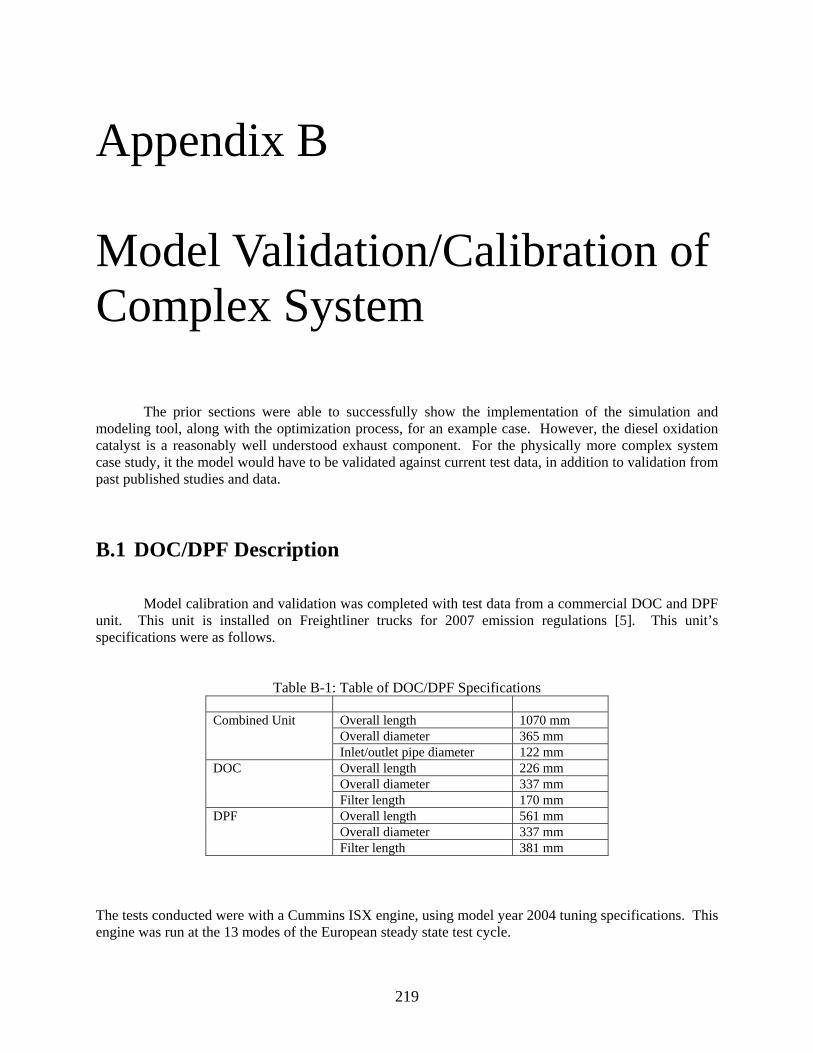
Appendix B . Model Validation/Calibration of Complex System
The prior sections were able to successfully show the implementation of the simulation and
modeling tool, along with the optimization process, for an example case. However, the diesel oxidation catalyst is a reasonably well understood exhaust component. For the physically more complex system case study, it the model would have to be validated against current test data, in addition to validation from past published studies and data.
B.1 DOC/DPF Description
Model calibration and validation was completed with test data from a commercial DOC and DPF unit. This unit is installed on Freightliner trucks for 2007 emission regulations [5]. This unit’s specifications were as follows.
Table B-1: Table of DOC/DPF Specifications
Overall length 1070 mm Overall diameter 365 mm
Combined Unit
Inlet/outlet pipe diameter 122 mm Overall length 226 mm Overall diameter 337 mm
DOC
Filter length 170 mm Overall length 561 mm Overall diameter 337 mm
DPF
Filter length 381 mm The tests conducted were with a Cummins ISX engine, using model year 2004 tuning specifications. This engine was run at the 13 modes of the European steady state test cycle.
219

Table B-2: Table of Engine Specifications Type: Cummins ISX 475, 15.0 liter, 6 cylinder, in-line. Rated Power: 475 bhp Rated Torque: 1650 lb-ft peak torque at 1200 rpm Speed: 2000 rpm governed speed
Table B-3: Table of Test Configurations Mode Speed (RPM) Torque (lb-ft) Emissions Euro 1 600 0 Pre/Post Euro 2 1250 1247 Pre/Post Euro 3 1500 624 Pre/Post Euro 4 1500 936 Pre/Post Euro 5 1250 624 Pre/Post Euro 6 1250 936 Pre/Post Euro 7 1250 312 Pre/Post Euro 8 1500 1247 Pre/Post Euro 9 1500 312 Pre/Post Euro 10 1750 1247 Pre/Post Euro 11 1750 312 Pre/Post Euro 12 1750 936 Pre/Post Euro 13 1750 624 Pre/Post Custom 1 600 0 Pre/Post Custom 2 600 312 Pre/Post Custom 3 1200 62 Pre/Post Custom 4 800 0 Pre/Post Custom 5 800 312 Pre/Post Custom 6 800 624 Pre/Post Custom 7 1000 0 Pre/Post
Table B-4: Table of Collected Particulate Mass Data Mode Time Sample Volume Euro 1 (Warmup) 30 min 0.4 SCFM of exhaust flow Euro 2 30 min 0.4 SCFM of exhaust flow Euro 4 30 min 0.4 SCFM of exhaust flow Euro 6 30 min 0.4 SCFM of exhaust flow Euro 8 30 min 0.4 SCFM of exhaust flow Euro 10 30 min 0.4 SCFM of exhaust flow Euro 12 30 min 0.4 SCFM of exhaust flow Custom 5 30 min 0.4 SCFM of exhaust flow
220

Table B-5: Table of Collected Data, pre and post rack emissions measurements Engine speed rpm Engine Torque N-m Engine Power kW AF ratio exhaust calculated unitless AF ratio measured unitless FA ratio exhaust calculated unitless FA ratio measured unitless Ambient temperature deg. C Barometric pressure kPaA Brake specific CO - Rack Emissions g/kW-hr Brake specific fuel consumption kg/kW-hr Brake specific HC – Rack Emissions g/kW-hr Brake specific NOx – Rack Emissions g/kW-hr DOC inlet exhaust gas temperature deg. C DPF outlet exhaust gas temperature deg. C DPF pressure drop (calculated) Pa DPF inlet pressure Pa DPF inlet exhaust gas temperature deg. F DPF outlet pressure Pa Catalyst valve position (indicates pre/post Rack Emissions) % Charge air temperature deg. C CO2 concentration, measured from AF ratio % CO2 concentration – Rack Emissions % CO concentration – Rack Emissions ppm Exhaust mass flow (wet) kg/min Exhaust out pressure Pa Exhaust stack (tail pipe) Temperature deg. C Exhaust volumetric flow (wet) m^3/min Fuel rate kg/min HC concentration (Rack Emissions) ppm HC concentration (Rack Emissions, Dry) ppm Intake air mass flow (dry) kg/min Intake air mass flow (wet) kg/min Intake air volume flow m^3/min Intake air volume flow (dry) m^3/min NOx + HC concentration sum ppm NOx concentration (Rack Emissions) ppm NOx concentration (Rack Emissions, wet) ppm NOx concentration (wet) ppm O2 concentration (Rack Emissions) % Turbine outlet pressure Pa Turbine outlet Temperature deg. C
221
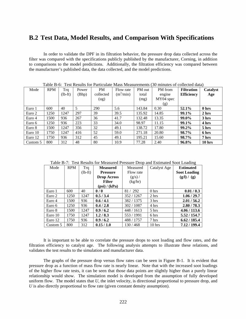
B.2 Test Data, Model Results, and Comparison With Specifications
In order to validate the DPF in its filtration behavior, the pressure drop data collected across the filter was compared with the specifications publicly published by the manufacturer, Corning, in addition to comparisons to the model predictions. Additionally, the filtration efficiency was compared between the manufacturer’s published data, the data collected, and the model predictions.
Table B-6: Test Results for Particulate Mass Measurements (30 minutes of collected data) Mode RPM Trq
(lb-ft) Power (Bhp)
PM collected
(ug)
Flow rate (m3/min)
PM out total (mg)
PM from engine
MY04 spec (g)
Filtration Efficiency
Catalyst Age
Euro 1 600 40 5 290 5.6 143.84 0.30 52.1% 0 hrs Euro 2 1250 1247 297 39 39.5 135.92 14.85 99.1% 2 hrs Euro 4 1500 936 267 36 41.7 132.48 13.35 99.0% 3 hrs Euro 6 1250 936 223 33 34.0 98.97 11.15 99.1% 4 hrs Euro 8 1500 1247 356 32 49.1 138.72 17.80 99.2% 5 hrs Euro 10 1750 1247 416 52 59.0 271.18 20.80 98.7% 6 hrs Euro 12 1750 936 312 45 49.1 195.21 15.60 98.7% 7 hrs Custom 5 800 312 48 80 10.9 77.28 2.40 96.8% 10 hrs
Table B-7: Test Results for Measured Pressure Drop and Estimated Soot Loading Mode RPM Trq
(lb-ft) Measured Pressure
Drop Across Filter
(psi) / (kPa)
Measured Flow rate
(g/s) / (kg/hr)
Catalyst Age Estimated Soot Loading
(g/l) / (g)
Euro 1 600 40 0 / 0 81 / 292 0 hrs 0.01 / 0.3 Euro 2 1250 1247 0.5 / 3.4 352 / 1267 2 hrs 1.06 / 29.7 Euro 4 1500 936 0.6 / 4.1 382 / 1375 3 hrs 2.01 / 56.2 Euro 6 1250 936 0.4 / 2.8 302 / 1087 4 hrs 2.80 / 78.3 Euro 8 1500 1247 0.9 / 6.2 448 / 1613 5 hrs 4.06 / 113.6 Euro 10 1750 1247 1.2 / 8.3 553 / 1991 6 hrs 5.52 / 154.7 Euro 12 1750 936 0.9 / 6.2 488 / 1757 7 hrs 6.62 / 185.4 Custom 5 800 312 0.15 / 1.0 130 / 468 10 hrs 7.12 / 199.4
It is important to be able to correlate the pressure drops to soot loading and flow rates, and the filtration efficiency to catalyst age. The following analysis attempts to illustrate these relations, and validates the test results to the simulation and manufacturer data.
The graphs of the pressure drop versus flow rates can be seen in Figure B-1. It is evident that pressure drop as a function of mass flow rate is nearly linear. Note that with the increased soot loadings of the higher flow rate tests, it can be seen that those data points are slightly higher than a purely linear relationship would show. The simulation model is developed from the assumption of fully developed uniform flow. The model states that U, the inlet velocity, is directional proportional to pressure drop, and U is also directly proportional to flow rate (given constant density assumption).
222

Pressure Drop versus Flow Rates
-1
0
1
2
3
4
5
6
7
8
9
0 100 200 300 400 500 600
Flow Rates (g/s)
Pres
sure
Dro
p (k
Pa)
Figure B-1: Pressure Drop Versus Flow Rate Data
The data can be divided into the high, medium, and low flow rate regimes. From this, the plots of
the pressure drop versus soot loading can be made, and is illustrated in Figure B-1. The behavior in this figure correlates reasonably well with the manufacturer’s published data for pressure drop and soot loading as shown in Figure B-2. Note that only the data for medium and high flow should be considered, as the low flow rate regime data did not have appropriate soot loadings to verify pressure drop versus soot loadings comparisons.
223

Pressure Drop versus Soot Loading
0
1
2
3
4
5
6
7
8
9
0 1 2 3 4 5 6 7 8
Soot Loading (g/l)
Pre
ssur
e Dr
op (k
Pa)
Low Flow Rates Medium Flow Rates High Flow Rates
Figure B-2: Pressure Drop Versus Soot Loading Data
The manufacturer’s published data shows a sharp increase in pressure drop during initial loading, and then a flatter, linear regime for high soot loadings. Although there aren’t enough data points from the test to confidently validate this, the fact that the pressure drop values were near the published data figures suggests a good agreement. Note that the manufacturer’s data is for a filter size of 5.8 liters and a cross sectional area of 285 cm^2. The filter tested had a 28 liter volume and a cross sectional area of 730 cm^2 (nearly 3 times as much as the manufacturer’s filter). Also note that the medium to high mass flow rate data measurements were equivalently 3 to 5 times as much as the manufacturer’s tested flow rates.
Figure B-3: Manufacturer Example Data on Pressure Drop versus Soot Loading [3]
224
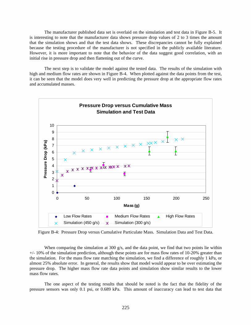
The manufacturer published data set is overlaid on the simulation and test data in Figure B-5. It is interesting to note that the manufacturer data shows pressure drop values of 2 to 3 times the amount that the simulation shows and that the test data shows. These discrepancies cannot be fully explained because the testing procedure of the manufacturer is not specified in the publicly available literature. However, it is more important to note that the behavior of the data suggest good correlation, with an initial rise in pressure drop and then flattening out of the curve.
The next step is to validate the model against the tested data. The results of the simulation with high and medium flow rates are shown in Figure B-4. When plotted against the data points from the test, it can be seen that the model does very well in predicting the pressure drop at the appropriate flow rates and accumulated masses.
Pressure Drop versus Cumulative MassSimulation and Test Data
0
1
23
4
5
6
78
9
10
0 50 100 150 200 250
Mass (g)
Pre
ssur
e Dr
op (k
Pa)
Low Flow Rates Medium Flow Rates High Flow RatesSimulation (450 g/s) Simulation (300 g/s)
Figure B-4: Pressure Drop versus Cumulative Particulate Mass. Simulation Data and Test Data.
When comparing the simulation at 300 g/s, and the data point, we find that two points lie within
+/- 10% of the simulation prediction, although these points are for mass flow rates of 10-20% greater than the simulation. For the mass flow rate matching the simulation, we find a difference of roughly 1 kPa, or almost 25% absolute error. In general, the results show that model would appear to be over estimating the pressure drop. The higher mass flow rate data points and simulation show similar results to the lower mass flow rates.
The one aspect of the testing results that should be noted is the fact that the fidelity of the pressure sensors was only 0.1 psi, or 0.689 kPa. This amount of inaccuracy can lead to test data that
225

cannot be effectively compared to the simulation. Therefore, given that the behavior of the model in addition to the precision of prediction is important, and the fact that the behavior matches well to prior results [24, 25, 26], as well as the manufacturer published data [3, 4], it can be said with confidence that the model is accurate to within the requirements of a sub-system of a larger system model.
Pressure Drop versus Cumulative MassManufacturer Data, Simulation Results, and Test Data
02468
101214161820
0 50 100 150 200 250
Mass (g)
Pres
sure
Dro
p (k
Pa)
Low Flow Rates Medium Flow RatesHigh Flow Rates Simulation (450 g/s)Simulation (300 g/s) Manufacturer Data Set 1 Manufacturer Data Set 2 Manufacturer Data Set 3
Figure B-5: Overlaid Data
Comparing the efficiency of filtration versus soot loading is more straightforward. The measured
efficiency of a clean filter at idle is about 50-60%. Once loaded, past 1 g/L, the efficiency improves dramatically to around 98-99%, in just about any operating condition, as can be seen in Figure B-6 and Figure B-7. The manufacturer’s published data also reflects this behavior in Figure B-7, particularly when looking at the 100/17 filter formulation. The simulation model results are shown in Figure B-6, and given the soot loading in g/L, the efficiency past 1 g/L matches well with published data as well as the testing results. Similarly to the behavior of a clean filter, the efficiency we find at low soot loadings is significantly less, and again matches both the manufacturer’s data and the testing data.
226

Figure B-6: Simulation Results for DPF Efficiency versus soot loading
Figure B-7: Manufacturer’s Data for DPF Efficiency versus soot loading [3]
227
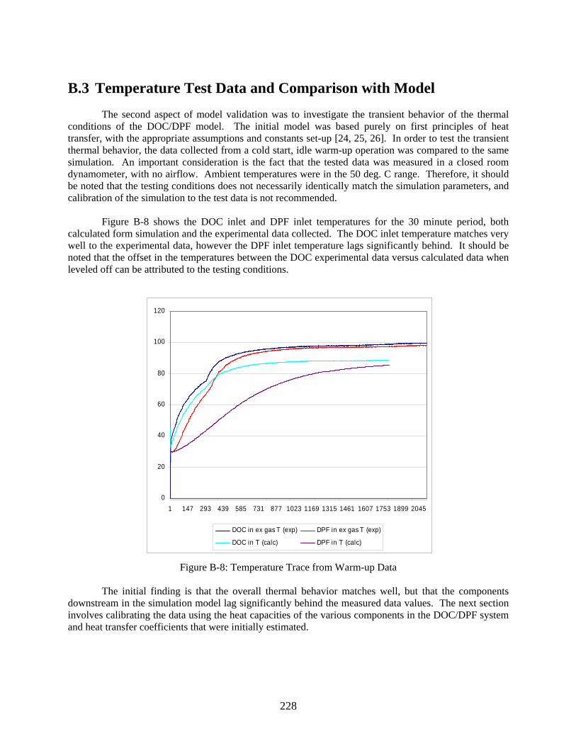
B.3 Temperature Test Data and Comparison with Model
The second aspect of model validation was to investigate the transient behavior of the thermal conditions of the DOC/DPF model. The initial model was based purely on first principles of heat transfer, with the appropriate assumptions and constants set-up [24, 25, 26]. In order to test the transient thermal behavior, the data collected from a cold start, idle warm-up operation was compared to the same simulation. An important consideration is the fact that the tested data was measured in a closed room dynamometer, with no airflow. Ambient temperatures were in the 50 deg. C range. Therefore, it should be noted that the testing conditions does not necessarily identically match the simulation parameters, and calibration of the simulation to the test data is not recommended.
Figure B-8 shows the DOC inlet and DPF inlet temperatures for the 30 minute period, both calculated form simulation and the experimental data collected. The DOC inlet temperature matches very well to the experimental data, however the DPF inlet temperature lags significantly behind. It should be noted that the offset in the temperatures between the DOC experimental data versus calculated data when leveled off can be attributed to the testing conditions.
0
20
40
60
80
100
120
1 147 293 439 585 731 877 1023 1169 1315 1461 1607 1753 1899 2045
DOC in ex gas T (exp) DPF in ex gas T (exp)
DOC in T (calc) DPF in T (calc)
Figure B-8: Temperature Trace from Warm-up Data The initial finding is that the overall thermal behavior matches well, but that the components
downstream in the simulation model lag significantly behind the measured data values. The next section involves calibrating the data using the heat capacities of the various components in the DOC/DPF system and heat transfer coefficients that were initially estimated.
228

B.4 Calibration Results for Temperatures
By increasing the heat transfer rate coefficient within the components of the DPF, as well as reducing the specific heat capacity of the DPF monolith, the simulation data was able to better match the tested data. Figure B-9 illustrates the component temperatures within the DPF.
Figure B-9: Simulation Temperature Trace for Warm-up Scenario
Figure B-10 and Figure B-11 show the temperatures of the monolith substrates and air temperatures in the DPF and DOC. The air temperature into the DPF matches significantly better with the tested results in Figure B-9.
Figure B-10: DPF Temperature Traces
229

Figure B-11: DOC Temperature Traces
Although calibration resulted in less thermal lag than before, it is important to realize that calibrating a general model to a specific test is not an accurate model validation method. By doing this, one effectively makes a highly accurate model only for those test conditions. This model is needed for a wide variety of different operating conditions. And changing the fundamental thermodynamic and heat transfer equations is not acceptable in this case. Instead, limited calibration that reduces the thermal lag in the system to better match our tested data suffices.
230