System AnalysisAdvisory Committee

Review

Michael SchilmoellerTuesday, September 27, 2011

2

Sources of Uncertainty

Scope of uncertainty

• Fifth Power Plan– Load requirements– Gas price– Hydrogeneration– Electricity price– Forced outage rates– Aluminum price– Carbon penalty– Production tax credits– Renewable Energy Credit

• Sixth Power Plan– aluminum price and

aluminum smelter loads were removed

– Power plant construction costs

– Technology availability– Conservation costs and

performance

3

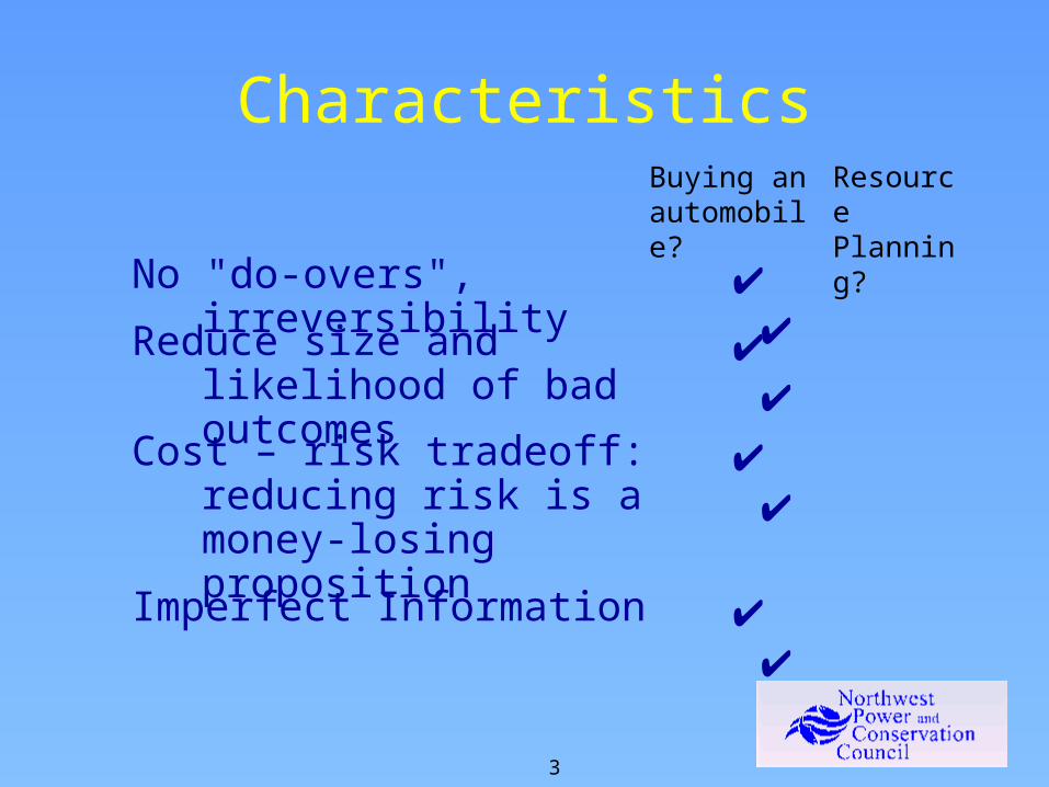
CharacteristicsResource Planning?

Reduce size and likelihood of bad outcomes

✔ ✔

Cost – risk tradeoff: reducing risk is a money-losing proposition

✔ ✔

Imperfect Information ✔ ✔

Buying an automobile?

No "do-overs", irreversibility

✔ ✔

4

CharacteristicsResource Planning?

Use of scenarios ✔ ✔

Resource allocations reflect likelihood of scenarios

✔ ✔

Resource allocations reflect severity of scenarios

✔ ✔

… even if "we cannot assign probabilities"

✔ ✔

Buying an automobile?

Some resources in reserve, used only if necessary

✔ ✔

5

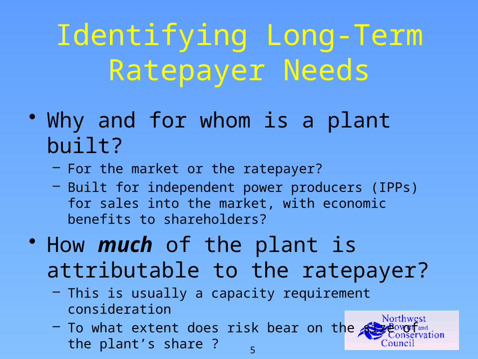
Identifying Long-Term Ratepayer Needs

• Why and for whom is a plant built?– For the market or the ratepayer?– Built for independent power producers (IPPs) for sales into the

market, with economic benefits to shareholders?

• How much of the plant is attributable to the ratepayer?– This is usually a capacity requirement consideration– To what extent does risk bear on the size of the plant’s share ?

6

How the RPM Differs fromOther Planning Models

• No perfect foresight, use of decision criteria for capacity additions

• Likelihood analysis of large sources of risk (“scenario analysis”)

• Adaptive plans that respond to futures

7

Excel Spinner Graph Model

• Represents one plan responding under each of 750 futures

• Illustrates “scenario analysis on steroids”

8

Modeling Process

The portfolio model

Likeli

hood

(Pro

babil

ity) Avg Cost

10000 12500 15000 17500 20000 22500 25000 27500 30000 32500

Power Cost (NPV 2004 $M)->

Risk = average ofcosts> 90% threshold

Likeli

hood

(Pro

babil

ity) Avg Cost

10000 12500 15000 17500 20000 22500 25000 27500 30000 32500

Power Cost (NPV 2004 $M)->

Risk = average ofcosts> 90% threshold

Likeli

hood

(Pro

babil

ity) Avg CostAvg Cost

10000 12500 15000 17500 20000 22500 25000 27500 30000 3250010000 12500 15000 17500 20000 22500 25000 27500 30000 32500

Power Cost (NPV 2004 $M)->

Risk = average ofcosts> 90% threshold

9

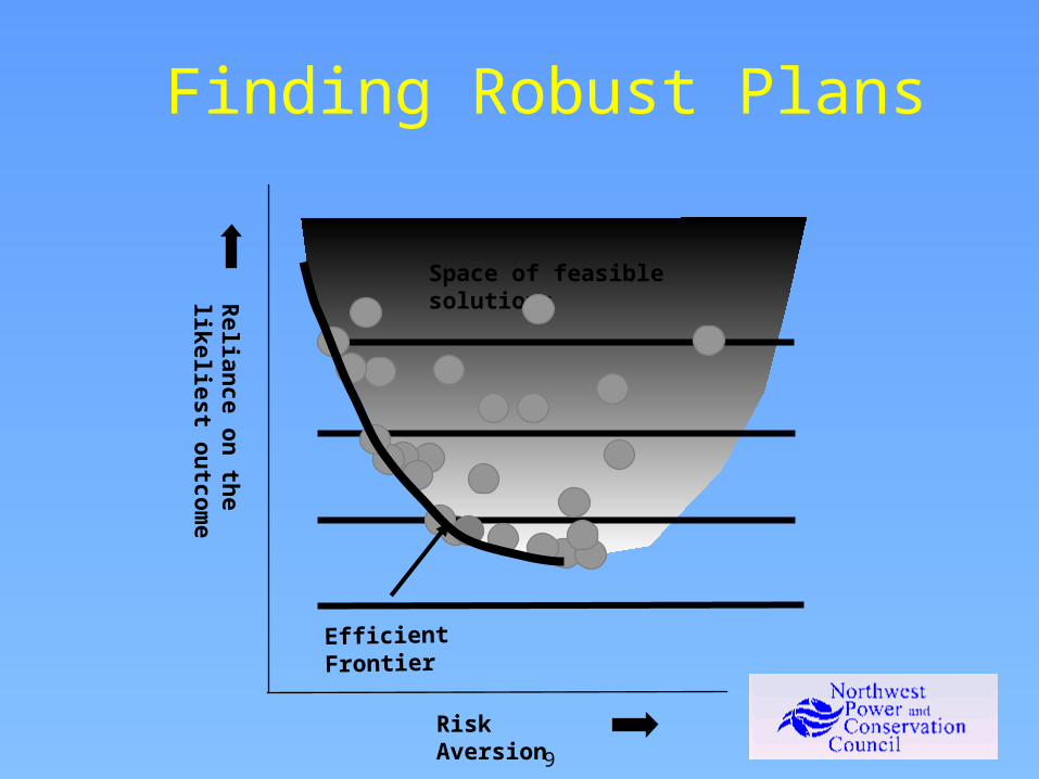
Space of feasible solutions

Finding Robust Plans

Reliance on the likeliest outcom

e

Risk Aversion

Efficient Frontier

10

Impact on NPV Costs and Risk

0

10

20

30

40

50

60

70

80

9030

40

50

60

70

80

90

100

110

120

130

140

150

160

170

180

190

200

210

220

230

Freq

uenc

y

Billions of 2006 Constant Dollars

NPV 20-Year Study Costs

Scope of uncertainty

C:\Documents and Settings\Michael Schilmoeller\Desktop\NWPCC - Council\SAAC\Presentation materials\L813 NPV Costs.xlsm

11

Decision Trees• Estimating the number of branches

– Assume possible 3 values (high, medium, low) for each of 9 variables, 80 periods, with two subperiods each; plus 70 possible hydro years, one for each of 20 years, on- and off-peak energy determined by hydro year

– Number of estimates cases, assuming independence: 6,048,000

• Studies, given equal number k of possible values for n uncertainties:

• Impact of adding an uncertainty:

Decision trees & Monte Carlo simulation

iesuncertaint values, ,, nkkN nkn

kN

N

kn

kn

,

,1

12

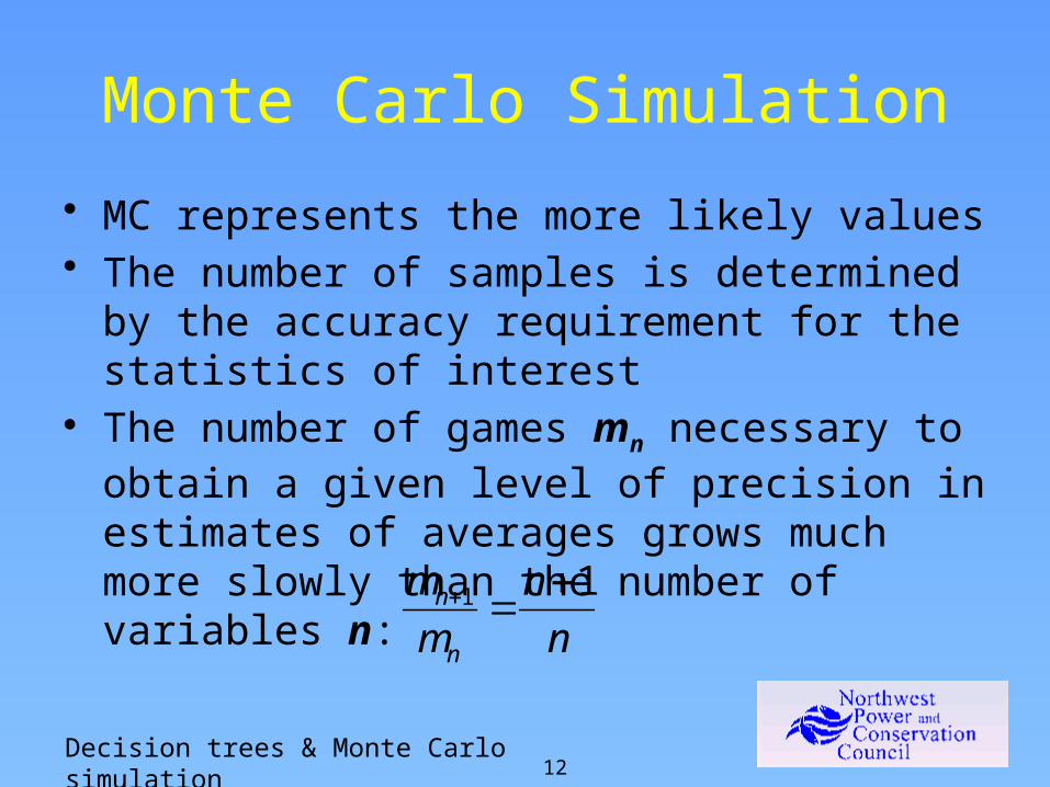
Monte Carlo Simulation• MC represents the more likely values• The number of samples is determined by the

accuracy requirement for the statistics of interest• The number of games mn necessary to obtain a

given level of precision in estimates of averages grows much more slowly than the number of variables n:

Decision trees & Monte Carlo simulation

nn

mm

n

n 11

13

Monte Carlo Samples

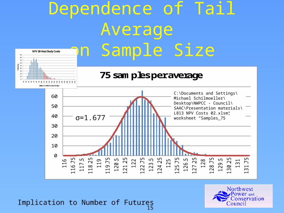
• How many samples are necessary to achieve reasonable cost and risk estimates?

• How precise is the sample mean of the tail, that is, TailVaR90?

Implication to Number of Futures

14

Assumed Distribution

0123456789

10111213141516

109

115

121

127

133

139

145

151

157

163

169

175

181

187

193

199

205

211

217

223

Freq

uenc

y

Billions of 2006 Constant Dollars

Tail Risk

Implication to Number of Futures

C:\Documents and Settings\Michael Schilmoeller\Desktop\NWPCC - Council\SAAC\Presentation materials\L813 NPV Costs 02.xlsm

15Implication to Number of Futures

Dependence of Tail Average on Sample Size

0

10

20

30

40

50

60

70

116

116.

7511

7.5

118.

2511

911

9.75

120.

512

1.25

122

122.

7512

3.5

124.

2512

512

5.75

126.

512

7.25

128

128.

7512

9.5

130.

2513

113

1.75

75 samples per average

C:\Documents and Settings\Michael Schilmoeller\Desktop\NWPCC - Council\SAAC\Presentation materials\L813 NPV Costs 02.xlsm, worksheet “Samples_75”

σ=1.677

0

10

20

30

40

50

60

70

80

90

30

40

50

60

70

80

90

100

110

120

130

140

150

160

170

180

190

200

210

220

230

Freq

uenc

y

Billions of 2006 Constant Dollars

NPV 20-Year Study Costs

16

Accuracy and Sample Size• Estimated accuracy of TailVaR90 statistic is

still only ± $3.3 B (2σ)!*

0

10

20

30

40

50

60

70

80

90

30

40

50

60

70

80

90

100

110

120

130

140

150

160

170

180

190

200

210

220

230

Freq

uenc

y

Billions of 2006 Constant Dollars

NPV 20-Year Study Costs

Implication to Number of Futures

0

10

20

30

40

50

60

70

116

116.

7511

7.5

118.

25 119

119.

7512

0.5

121.

25 122

122.

7512

3.5

124.

25 125

125.

7512

6.5

127.

25 128

128.

7512

9.5

130.

25 131

131.

75

75 samples per average

*Stay tuned to see why the precision is actually 1000x better than this!

17

Accuracy Relative to the Efficient Frontier

123200

124200

125200

126200

127200

128200

129200

77000 78000 79000 80000 81000 82000 83000

Ris

k (N

PV $

2006

M)

Cost (NPV $2006 M)

L813

L813 L813 Frontier

C:\Backups\Plan 6\Studies\L813\Analysis of Optimization Run_L813vL811.xls

Implication to Number of Futures

18

Finding the Best Plan

• Each plan is exposed to exactly the same set of futures, except for electricity price

• Look for the plan that minimizes cost and risk

• Challenge: there may be many plans (Sixth Plan possible resource portfolios:1.3 x 1031)

Implication to Number of Plans

19

Space of feasible solutions

The Set of Plans Precedes the Efficient Frontier

Reliance on the likeliest outcom

e

Risk Aversion

Efficient Frontier

Implication to Number of Plans

20

Finding the “Best” Plan

155600

155800

156000

156200

156400

156600

156800

157000

0 500

1000

1500

2000

2500

3000

3500

4000

4500

5000

5500

6000

6500

7000

7500

8000Ta

ilVar

90 ($

M N

PV)

simulation number

Reduction in TailVar90with increasing

simulations (plans)

C:\Documents and Settings\Michael Schilmoeller\Desktop\NWPCC - Council\SAAC\Presentation materials\Asymptotic reduction in risk with increasing plans.xlsm

Implication to Number of Plans

21

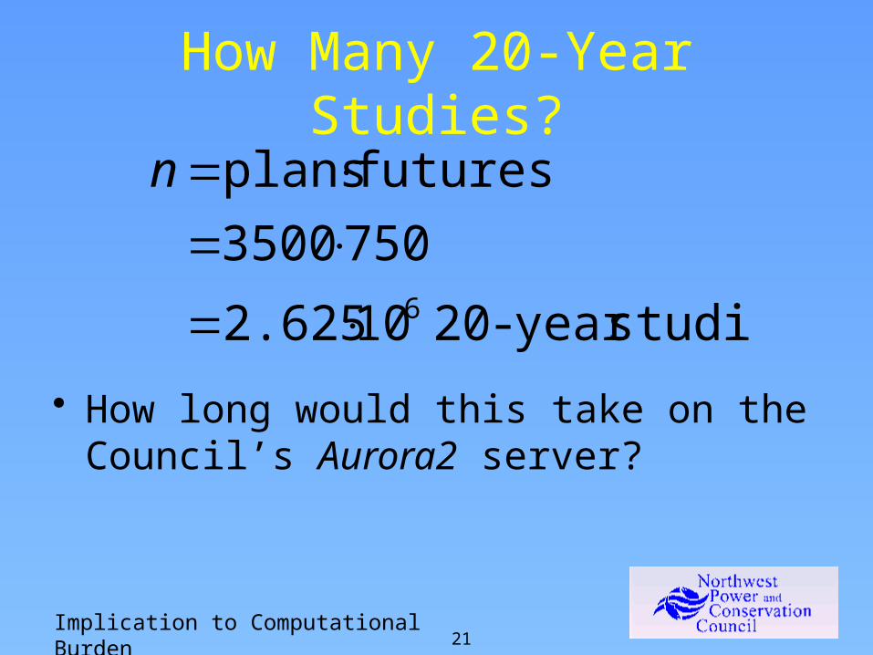
How Many 20-Year Studies?

• How long would this take on the Council’s Aurora2 server?

studiesyear -20 10 2.625

750 3500 futures plans

6

n

Implication to Computational Burden

22

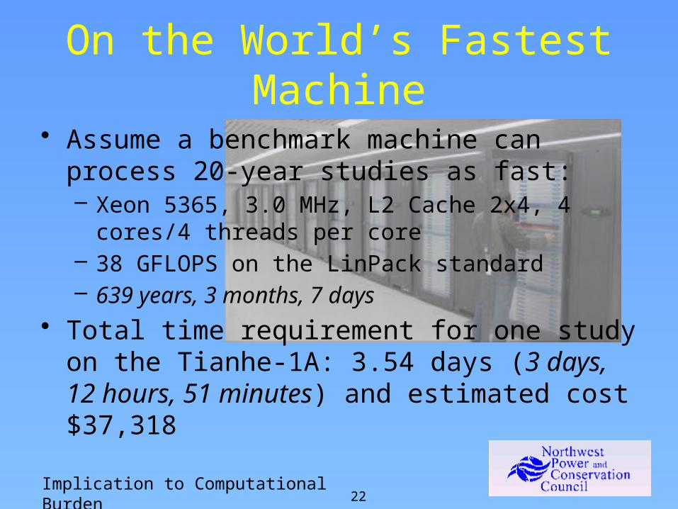
• Assume a benchmark machine can process 20-year studies as fast:– Xeon 5365, 3.0 MHz, L2 Cache 2x4, 4 cores/4

threads per core– 38 GFLOPS on the LinPack standard– 639 years, 3 months, 7 days

• Total time requirement for one study on the Tianhe-1A: 3.54 days (3 days, 12 hours, 51 minutes) and estimated cost $37,318

On the World’s Fastest Machine

Implication to Computational Burden

23

How the RPM Satisfies the Requirements of a Risk Model• Statistical distributions of hourly data

– Estimating hourly cost and generation– Application to limited-energy resources– The price duration curve and the revenue curve

• Valuation costing• An open-system models• Unit aggregation• Performance and precision

24

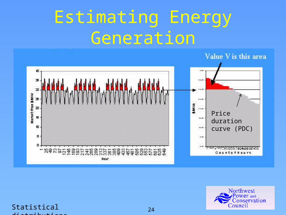
Estimating Energy Generation

Price duration curve (PDC)

Statistical distributions

25

Gross Value of Resources Using Statistical Parameters of

Distributions

e

ee

ge

ee

g

e

ge

dd

ppd

(h))(p

pp

NN

dNpdNpc

12

1

21

2/)/ln(

ln ofdeviation standard is

price gas theis pricey electricit average theis

variablerandom )1,0( afor CDF theis where

(4) )()( Assumes:1) prices are

lognormally distributed

2) 1MW capacity

3) No outages

V

Statistical distributions

26

Estimating Energy Generation

*

*

1)(CDFcf

)(CDF

Calculus) of Thm (Fund

)(CDF

*

*

gg

gg

g

ppgHg

gH

ppg

e

P

eH

pV

NCp

pNCpV

dppNCV

Applied to equation (4), this gives us a closed-form evaluation of the capacity factor and energy.

Statistical distributions

27

Implementation in the RPM

• Distributions represent hourly prices for electricity and fuel over hydro year quarters, on- and off-peak– Sept-Nov, Dec-Feb, Mar-May, June-Aug– Conventional 6x16 definition– Use of “standard months”

• Easily verified with chronological model• Execution time <30µsecs• 56 plants x 80 periods x 2 subperiods

Statistical distributions

28

Energy-Limited Dispatch

Statistical distributions

29

“Valuation” CostingComplications from correlation of fuel price, energy, market prices

priceLoads (solid) & resources (grayed)

Valuation Costing

)( imi

im ppqQpc åOnly correlations are now those with the market

30

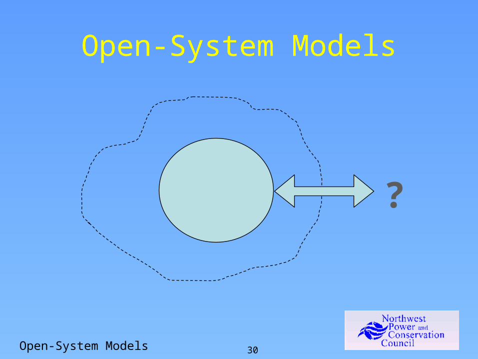
Open-System Models

?

Open-System Models

31

Modeling Evolution• Problems with open-system production cost

models– valuing imports and exports– desire to understand the implications of events

outside the “bubble”• As computers became more powerful and less

expensive, closed-system hourly models became more popular– better representation of operational costs and

constraints (start-up, ramps, etc.)– more intuitive

Open-System Models

32

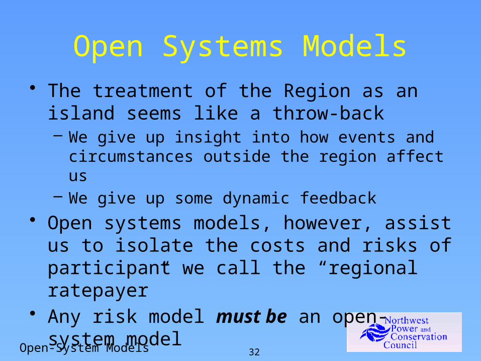
Open Systems Models• The treatment of the Region as an island seems

like a throw-back– We give up insight into how events and

circumstances outside the region affect us– We give up some dynamic feedback

• Open systems models, however, assist us to isolate the costs and risks of participant we call the “regional ratepayer”

• Any risk model must be an open-system model

Open-System Models

33

The Closed- Electricity System Model

fuel price+εi

dispatchprice

energygeneration

energyrequire-ments

market price +εi for electricity

Only one electricity price balances requirements and generation

• If fuel price is the only “independent” variable, the assumed source of uncertainty, electricity price will move in perfect correlation

• That is, outside influences drive the results• We are back to an open system

Open-System Models

34

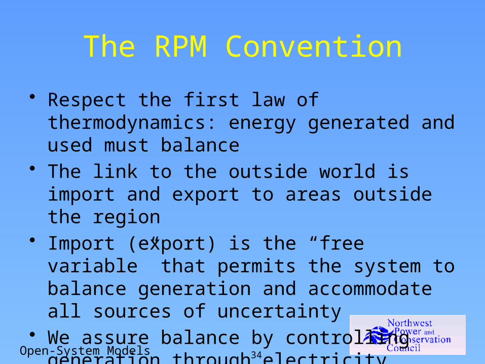
The RPM Convention• Respect the first law of thermodynamics: energy

generated and used must balance• The link to the outside world is import and export

to areas outside the region• Import (export) is the “free variable” that permits

the system to balance generation and accommodate all sources of uncertainty

• We assure balance by controlling generation through electricity price. The model finds a suitable price by iteration.

Open-System Models

35

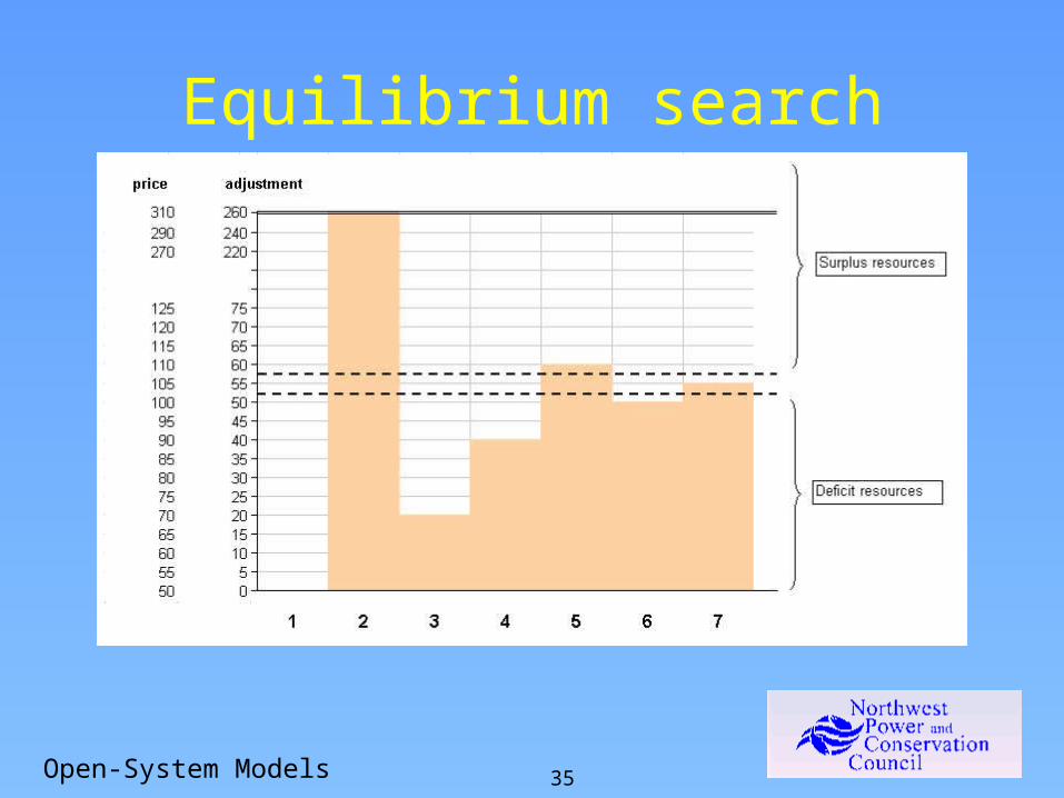
Equilibrium search

Open-System Models

36

Unit Aggregation

0.00

2.00

4.00

6.00

8.00

10.00

12.00

4000 5000 6000 7000 8000 9000 10000 11000 12000 13000 14000 15000 16000 17000

VOM

($/M

Wh)

Heat Rate (BTU/kWh)

West 1 West 2 West 3

West 4 Beaver East 4

East 5 East 7 East 8

Hermiston Ignore East 1

• Forty-three dispatchable regional gas-fired generation units are aggregated by heat rate and variable operation cost

• The following illustration assumes $4.00/MMBTU gas price for scaling

Source: C:\Backups\Plan 6\Studies\Data Development\Resources\Existing Non-Hydro\100526 Update\Cluster_Chart_100528_183006.xls

Unit Aggregation

37

Cluster Analysis

1130

1219

1305

1290

1131

1246

1247

1248

1021 10

410

2014

6714

6816

5016

5111

9811

9912

0112

02 1023

1136

1028

1475

1443

1368

1200

1228

1089 15

7114

1110

0012

0412

03 100

1054

1797

1291

1292

1402

1403

01

23

45

Dendrogram of agnes(x = Both_Units, diss = FALSE, metric = "manhattan", stand = TRUE)

Agglomerative Coefficient = 0.98Both_Units

Hei

ght

Source: C:\Backups\Plan 6\Studies\Data Development\Resources\Existing Non-Hydro\100526 Update\R Agnes cluster analysis\Cluster Analysis on units.doc

Unit Aggregation

38

Performance• The RPM performs a 20-year simulation of one plan

under one future in 0.4 seconds• A server and nine worker computers provide

“embarrassingly parallel” processing on bundles of futures. A master unit summarizes and hosts the optimizer.

• The distributed computation system completes simulations for one plan under the 750 futures in 30 seconds

• Results for 3500 plans (2.6 million 20-year studies) require about 29 hours

Performance and Precision

39

Precision

Source: email from Schilmoeller, Michael, Monday, December 14, 2009 12:01 PM, to Power Planning Division, based on Q:\SixthPlan\AdminRecord\t6 Regional Portfolio Model\L812\Analysis of Optimization Run_L812.xls

Performance and Precision

40

Choice of Excel as a Platform• The importance of transparency and

accessibility, availability of diagnostics• Olivia• The ability of Olivia to write VBA code for

the model• RPM’s layout of data and formulas • High-performance Excel

– XLLs– Carefully controlled calculations

• System requirements• Crystal Ball and CB Turbo

41

…And From the Last Meeting,May 19, 2011 …

42

What do the Risky Futures Look Like?

• See Appendix J of the Sixth Power Plan– Section Quantitative Risk Analysis identifies

electricity prices, loads, carbon penalty, and natural gas prices to be the principal sources of risk

Risky Futures

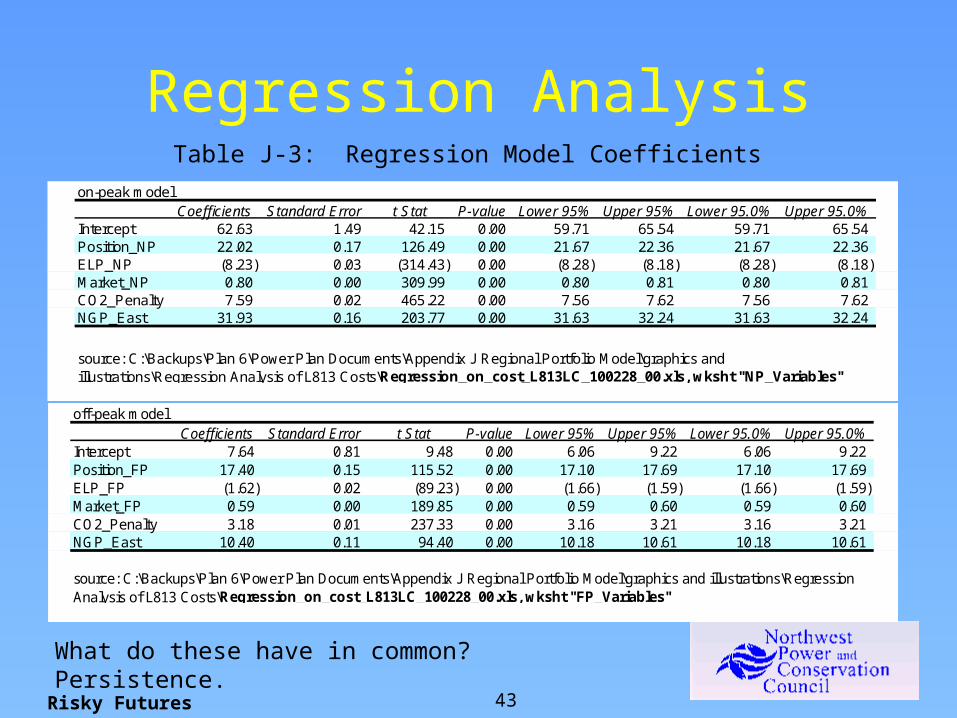
43

Regression AnalysisTable J-3: Regression Model Coefficients

on-peak modelCoefficients Standard Error t Stat P-value Lower 95% Upper 95% Lower 95.0% Upper 95.0%

Intercept 62.63 1.49 42.15 0.00 59.71 65.54 59.71 65.54 Position_NP 22.02 0.17 126.49 0.00 21.67 22.36 21.67 22.36 ELP_NP (8.23) 0.03 (314.43) 0.00 (8.28) (8.18) (8.28) (8.18) Market_NP 0.80 0.00 309.99 0.00 0.80 0.81 0.80 0.81 CO2_Penalty 7.59 0.02 465.22 0.00 7.56 7.62 7.56 7.62 NGP_East 31.93 0.16 203.77 0.00 31.63 32.24 31.63 32.24

source: C:\Backups\Plan 6\Power Plan Documents\Appendix J Regional Portfolio Model\graphics and illustrations\Regression Analysis of L813 Costs\Regression_on_cost_L813LC_100228_00.xls, wksht "NP_Variables"

off-peak modelCoefficients Standard Error t Stat P-value Lower 95% Upper 95% Lower 95.0% Upper 95.0%

Intercept 7.64 0.81 9.48 0.00 6.06 9.22 6.06 9.22 Position_FP 17.40 0.15 115.52 0.00 17.10 17.69 17.10 17.69 ELP_FP (1.62) 0.02 (89.23) 0.00 (1.66) (1.59) (1.66) (1.59) Market_FP 0.59 0.00 189.85 0.00 0.59 0.60 0.59 0.60 CO2_Penalty 3.18 0.01 237.33 0.00 3.16 3.21 3.16 3.21 NGP_East 10.40 0.11 94.40 0.00 10.18 10.61 10.18 10.61

source: C:\Backups\Plan 6\Power Plan Documents\Appendix J Regional Portfolio Model\graphics and illustrations\Regression Analysis of L813 Costs\Regression_on_cost_L813LC_100228_00.xls, wksht "FP_Variables"

What do these have in common? Persistence.

Risky Futures

44

Intuition About Risk

• Worst Futures Spinner.xls• Noticed that high-cost (high-risk) futures

are high-load futures• Began our discussion of unit-energy

costs

Risky Futures

45

Uses and Abuses ofthe Efficient Frontier

123

124

125

126

127

128

129

77 78 79 80 81 82 83

Thou

sand

s

Thousands

Side Effects

Inef

fect

ive

source: \EUCI 100323 Presentation\Efficient Frontier\EUCI 100323 01.xls

Efficient Frontier

46

Efficient Frontier

• Provides an alternative to weighting– Easily constructed– General application

• Preserves the trade-off decision

Efficient Frontier

47

What does the Efficient Frontier Tell Us?• The Efficient Frontier does not

tell us what to do• The Efficient Frontier tells us

what not to do• Most useful if there are a large

number of choices

Efficient Frontier

48

Fooled by the Graph• Error 1: The geometry of the

points on the efficient frontier has meaning or otherwise provides guidance, or equivalently …

• There exists a formula or other objective means for determining an optimal point on the efficient frontier

Abusing the EF

49 49

Unclear About Control• Error 2: The “expected cost” on the

efficient frontier is controllable, equivalently …

• We can “buy” risk reduction with the increase in expected costs

Abusing the EF

50

Mislead by Averages

• Error 3: “We know what ‘expected cost’ means.”

• In fact, there are many different ways to compute an average, and they all have different meanings.

• More important, the average of a distribution may be very meaningful in one situation and meaningless in another.

• Example of “average” SCCT dispatch across futures of a low-risk portfolio

Abusing the EF

51

Conservation Representation

• The construction of conservation supply curves

• Discretionary and lost opportunity

• Fifth Power Plan findings• Conservation risk premium

• Sources of premium value …• Sixth Power Plan findings …

Conservation

52

Sources of Premium Value

• Capacity deferral• Protection from fuel and electricity price

excursions, in particular due to carbon risk• Short-term price reduction• Purchases at below-average prices

(“dollar-cost averaging”)• Opportunity to develop and resell

conservation energyC:\Backup\Plan 5\Portfolio Work\Olivia\SAAC 2010\110519 SAAC Meeting\Conservation Premium\The sources of premium value 101206 1600.lnk

Conservation

53

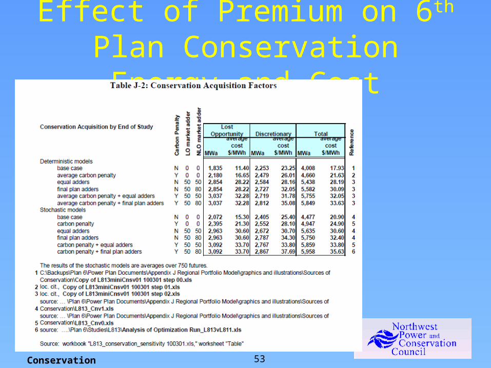
Effect of Premium on 6th Plan Conservation Energy and Cost

Conservation

54

Crystal Ball Decision Cells and the Resource Portfolio (“Plan”)

55

End