synthetic population generation at disaggregated...

168

Transportation Research Record: Journal of the Transportation Research Board, No. 2429, Transportation Research Board of the National Academies, Washington, D.C., 2014, pp. 168–177.DOI: 10.3141/2429-18

The execution of agent-based microsimulation requires an initial set of agents with detailed socioeconomic and demographic attributes to support subsequent behavioral and market models. Data limitations and privacy reasons often restrict the scope and detail with which a synthetic population can be generated by the traditional population synthesis approach. For the accommodation of the growing requirement of microsimulation on spatial resolution and variety, considering new data sources that overcome the data limitations and support population synthesis at more disaggregated levels is necessary. This paper presents a two-stage population synthesis approach not only to improve the accu-racy of population generation with imperfect microdata and marginal data, but also to use additional data sets when the spatial details of the synthetic population are interpolated. A general iterative proportional fitting (IPF) method is used in the first stage to estimate the joint dis-tribution of household and individual characteristics under multiple levels of constraints. Additional building information is collected from multiple sources and used to estimate spatial patterns of housing and household characteristics that are then preserved through a second IPF procedure. Preliminary tests of the proposed two-stage IPF-based approach with Singapore data show that the method yields better fitted population realizations at more fine-grained levels than do traditional one-step population synthesis methods.

In the past decade growing efforts have been seen in the development of an agent-based microsimulation platform for activity-based travel demand models as well as large-scale land use and transportation models, including MATSim (1), DynaMIT (2), UrbanSim (3), and ILUTE (4) as well as others (5, 6). These models generally require complete lists of agents such as households, persons, and firms to be initialized with realistic attributes, locations, relationships, and behaviors at the beginning of the simulation.

Although in most cases detailed information of the full population can be found in the census data, privacy reasons and policy restric-tions usually make the data inaccessible to researchers. Thus, popu-lation synthesis approaches were developed to combine microdata samples that lacked spatial detail with marginal data about population

characteristics at aggregated spatial levels to expand the microdata sample into a complete synthetic population.

The quality of generated synthetic populations depends, of course, on the quality and detail of the sample and marginal data. While the data quality has been improving, it has not kept pace with the growing interest in microsimulations at the scale of buildings and individu-als tagged with many associated characteristics. Available sample data are often thin and incomplete, and the available marginals are spatially aggregated. Even in those countries with sizable microdata samples, the geographic resolution of the released data remains coarse (for privacy reasons). In this paper a population synthesis approach is presented that is intended to improve the attribute richness and geographic distribution of synthetic populations generated from typi-cally available marginal statistics combined with supplemental data about built form and population density. Disaggregated synthetic population realizations are generated at the building and parcel levels, and marginal constraints on household and population counts are also considered.

The standard iterative proportional fitting (IPF) algorithm used by many earlier population synthesizers is not able to fit marginal constraints on multiple agent types simultaneously. For example, an agent-based model may want to simulate the behavior of individual agents as well as households agents. There are likely to be separate marginal statistics for household characteristics and population char-acteristics, together with limited cross-tabulation statistics about individual within-household characteristics. The usual IPF algorithm must be modified to combine the household and population fitting procedures in a way that retains some of the structure of the joint distribution that is evident in the cross tabulations. The synthesizer proposed in this paper addresses the geographic resolution and the household and population interaction issues with a single multi stage IPF procedure. The approach has been implemented for the SimMobility project in the Future Urban Mobility research group at the Singapore–MIT [Massachusetts Institute of Technol-ogy] Alliance for Research and Technology (SMART) in Singapore. SimMobility is an integrated system of mobility-sensitive simulation models to evaluate future urban transportation scenarios. (For more information on the SimMobility project research, see http://ltaacademy.gov.sg/doc/J10Nov-p30Ben-Akiva_FutureUrbanMobility.pdf.)

The rest of the paper is organized as follows. A review of the previous research effort on relevant issues of population synthesis is presented next, followed by a presentation of the theoretical devel-opment of the general IPF procedure that enables satisfying multi-level constraints simultaneously in the fitting process. The proposed two-stage population synthesis approach is then discussed, applied to the Singapore case, and evaluated on the basis of a series of tests. Conclusions are developed to close the paper.

Synthetic Population Generation at Disaggregated Spatial Scales for Land Use and Transportation Microsimulation

Yi Zhu and Joseph Ferreira, Jr.

Y. Zhu, Room 7-534, and J. Ferreira, Jr., Room 9-532, Department of Urban Studies and Planning, Massachusetts Institute of Technology, 77 Massachusetts Avenue, Cambridge, MA 02139. Corresponding author: Y. Zhu, [email protected].

Zhu and Ferreira 169

Previous Work

In the field of urban and transportation modeling, Beckman et al. are among the researchers who first proposed to combine aggregated control totals from the census summary files and detailed micro-data from Public Use Microdata Sample data to generate a complete population of households with critical attributes (7). To estimate the joint distribution of agent attributes under constraints of marginal distributions, they used the standard IPF procedure initially developed by Deming and Stephan (8), and later improved by Stephan (9), Fienberg (10), Ireland and Kullback (11), and others.

Grounded on the work of Beckman et al. (7), research on popula-tion generation has, for years, been striving to address a number of issues related to population synthesis, ranging from zero-cell problems (12, 13) to nonconforming constraints (14) to spatial heterogeneity (15). In this review, the focus is on recent efforts to address two key issues:

1. Generating multiple agent types simultaneously and2. Addressing data incompleteness.

Population synthesis for Multiple Agent Types

Mainly four groups of methods have recently been proposed to address Issue 1. The first group estimates the joint distribu-tions of attributes for households and persons through separate IPF procedures. Then, household samples are drawn into the synthetic population iteratively according to how well the types of house-holds and their members fit to the estimated joint distributions at household and person levels (13, 16). The second group of methods adopts a two-step fitting process that includes part of the first-step estimates in the second step. For example, Pritchard and Miller pro-posed a method that fits persons first and then uses a subset of the person type attributes (such as head gender or husband–wife type) with other household attributes to perform an IPF procedure at the household level (17). At the allocation stage, households and persons are matched through shared attributes included in both IPF procedures, and a conditional Monte Carlo method is used to assign persons to households.

The third group of methods focuses on incorporating individual marginal distributions into the marginal distributions of households. For example, ALBATROSS uses a two-step procedure with the first step converting known marginal distributions of persons to mar-ginal distributions of households on relevant attributes by using a relation matrix. In the relation matrix, the distribution of households across the attributes of individuals who live in a household is speci-fied. The resulting marginal household distributions are used as con-straints for the second-stage IPF, which produces a joint distribution of household attributes (12).

The IPF algorithms used in these first three groups of methods are mainly the standard ones, and the joint distributions of household-level attributes and person-level attributes are fitted either separately or sequentially. The fourth group of methods is intended to simultane-ously generate the joint distributions by satisfying household-level and person-level constraints. Ye et al. used an iterative reweight-ing procedure to heuristically adjust household weights to satisfy household-level and person-level joint distribution of attributes derived from separate IPF procedures separately (18). This method is analogous to a sparse list variant of the IPF procedure using

frequencies fitted by IPF of household types and person types as marginal constraints. However, as pointed out by the authors, the method is still heuristic in nature and there is no theoretical proof of convergence. By comparison, the hierarchical IPF method pro-posed by Müller and Axhausen is intended to satisfy multiple lev-els of constraints in a single IPF procedure (19). That method is similar to the general IPF algorithm used in this study. A detailed introduction and a discussion of the algorithm are presented in the following section.

Accounting for Data Limitations

To address the limitation of sample availability, Barthelemy and Toint develop a synthesis method working without samples based on a hierarchical three-step approach (20). The first step is to create individual pools based on known empirical distributions of individual attributes processed by a standard IPF procedure. Then, entropy maximization and Tabu search are used to generate household pools, and ad hoc matching rules are used in the third step to assign indi-viduals to households. However, this approach does not guarantee the consistency of households and individuals in satisfying marginal constraints.

In addition, a simulation-based approach was developed by Farooq et al. to address the data limitation issue (21). Gibbs sampling was used to produce the joint distribution of agents’ attributes based on a series of conditional distributions estimated on the basis of the limited observed data. However, Farooq et al.’s approach faces a critical challenge. As the number of constraint attributes increases, the complete conditionals that are required by Gibbs sampling will be increasingly unlikely to be available. The multinomial logit models used to estimate the conditional distributions may not have a satis-factory goodness of fit. As a result, inconsistencies will arise for the joint distribution of attributes obtained from estimated conditional distributions.

Both approaches generated populations with only those attributes that were included in the constraints. In this paper, there is a detailed sample with a small sampling rate (1%), and the aim is to seed a population with many attributes that are included in the sample but for which there are few or no marginal constraints (e.g., information about vehicle ownership, occupation, and lifestyle). It is in general impossible to constrain all attributes either because of the unknown marginal data of some attributes or because the dimensionality of the contingency table used for IPF is restricted by computer memory. Thus, both approaches are inadequate for the purposes of this paper. As data from emerging sources such as urban sensing and web ser-vices become increasingly available, the time has come to develop approaches that can extract useful information, such as workplaces and home locations, from these data to support population synthesis and microsimulation (22).

GenerAL iTerATive ProPorTionAL FiTTinG ALGoriThM For MuLTiPLe LeveL ConsTrAinTs

The problem of interest is to estimate the joint distribution of multi-dimensional attributes, in which relatively unreliable correlation information from the microdata sample is supplemented by reliable marginal subtotals obtained from independent sources. Deming and

170 Transportation Research Record 2429

Stephan proposed an objective function based on a weighted least squares criterion (8):

p

pi i

ii

ˆ 2

∑ ( )− π

subject to

r j Ji j

i j

ˆ for 1, 2, 3, . . . , (1)∑ π = = ∈

where

pi = sample proportion of cell i, π̂i = estimated cell proportion, j = index for attribute categories, and J = total number of categories of all constraint attributes.

Known marginal distributions rj for categories are applied for the minimization problem to restrict the estimation of π̂i. Because this problem cannot be solved directly, they proposed the standard IPF algorithm to find the estimator.

Later, Ireland and Kullback showed that the IPF estimators actually minimize the discrimination information (11):

l pp

ii

ii

ˆ; ˆ lnˆ

(2)∑( )π = ππ

where l(π̂; p)is the discrimination information function of the sample distribution π and the estimated distribution p. With the Lagrange multipliers method, the least squares estimates can be shown to take the following form:

pi

ij

j

J

∑( )π = −λ −lnˆ

1 (3)

where λj are multipliers corresponding to the linear constraints. Meanwhile they also showed that if the expansion factor α for category j in iteration t is defined by solving Σπ̂ i

t−1α jt = rj, when

t → ∞, α it → αi and

pi

i

ij

j

Jˆexp 1 (4)∑( )α =

π= −λ −

The work of Ireland and Kullback is important because it proved the convergence of the IPF procedure toward the estimate for the minimum discrimination information.

Along the same line, this algorithm can be expanded to satisfy mul-tiple levels of marginal constraints by counting the number of persons in each household with the constrained attribute. Then, Equation 1 can be rewritten as

p

pi i

ii

ˆ 2

∑ ( )− π

subject to

R r j Ji ij j

i j∑π = =

∈

ˆ for 1, 2, 3, . . . , (5)

When only one level of constraint needs to be satisfied, Rij indicates whether cell i belongs to category j. For the problem with multiple levels of constraints, Rij can be used to convert the cell values for households to corresponding individual-level estimates. Thus, Rij can be defined as

1 for and belongs to a household-levelattribute

for and belongs to an individual-levelattribute

0 otherwise

R

i j j

Lm

ni j jij

jj

=

∈

× ∈

where m is the number of agents that need to be estimated and nj is the number of agents of another type whose constraints j need to be satisfied jointly by the minimization. Lj is easy to obtain by converting attributes of one agent type to corresponding attributes of another agent type if the relationship between the two agent types is clear. For example, gender as an individual attribute can be con-verted to two separate household attributes (e.g., number of males and number of females in a household). Then, Lj is 1 if the category is one male, 2 if the category is two males, and so on.

Lagrange multipliers provide a way to find the local optimizer for the objective function (5). By transforming the equality constraints, Function 5 becomes

pR i Ii

ij j

j∑π + λ + = =ln

ˆ1 0 1, 2, 3, . . . , (6)

Rewriting the equality constraint as

pi Ii

ij

j

Rjˆexp 1 1, 2, 3, . . . , (7)∑π

= − λ −

=

allows one to find the estimators of π̂i by simultaneously solving the Lagrange factor parameters λj for all categories of household-level and individual-level constraints. It can also be seen that Equation 6 has a form similar to that of Equation 3, except for the constant Rj. Thus, it also can be solved by the IPF procedure. Now assume that αj = exp(−Σjλj − 1) again, then π̂i/pi = αj

Rj. According to Equation 4 and by analogy, it can be seen that the expansion factor is α j

Rj. Thus, in the iterative procedure, the expansion factor for category j of iteration t can be updated by solving

rit

jR t

jjˆ̂ (8)1∑ ( )π α =−

Note that π̂̂it−1 denotes the distribution of the agent type that is the same

as the one constrained by rj. Thus when rj is a marginal constraint applied to individuals, Equation 8 becomes

R rit

j jR t

j

i j

jˆ (9)1∑ ( )π α =−

∈

where π̂it−1 is the distribution of households.

In this case, to find the expansion factor, a nonlinear equation needs to be solved in each iteration when the agent type of constraint is different from the agent type being estimated by the IPF procedure. A more rigorous proof on convergence can be provided by following Ireland and Kullback (11). [Also see Farooq et al. (21).] That this IPF


approach is not intended to simultaneously fit joint distributions of characteristics of multiple agent types also needs to be made clear. Instead, it is intended to estimate the joint distributions of one agent type without violating constraints for other agent types that have associations with the estimated agents. The strength and limitation of this IPF procedure will be further discussed in the following sections.

New PoPulatioN SyNtheSiS aPProach

For the generation of a representative population at the most disaggregated level possible, a twostep population synthesis approach is proposed as in Figure 1:

1. Firststage IPF. Fit the joint distribution of selected household and individual attributes simultaneously for each spatial aggregation level at which reliable marginal totals are available through the general IPF method. Populate each disaggregated cell with the fitted number of households (and their full complement of attribute detail) by drawing randomly from those households in the microdata sample whose attributes match the marginal characteristics required for that cell.

2. Secondstage assignment. Locate each of these households at a more disaggregated spatial level by using a second IPF that tries to match the spatial variation estimated from the microdata sample and other available data.

As illustrated in Figure 1, at the second stage, the synthetic households generated from the first stage can be assigned to a more

disaggregated spatial level with the help of more spatially detailed marginal distributions, either obtained directly or estimated from available data sources. A detailed description for each of these steps is provided in the following.

Population Generation with aggregated Marginals estimating the Joint Distribution of households and individuals

Step 1.A is to use the general IPF method described in the previous section to estimate the joint distribution of households’ attributes taking into account the marginal constraints for selected individual attributes. Selected individual attributes are converted to the number of constituent members with corresponding attributes in households. The gender of individuals becomes the number of males and the number of females in households. As a result, each category of the individual attribute becomes a controlling attribute at the household level. Thus, when individual attributes having many categories are included as marginal constraints for householdlevel fitting, the dimensionality of the householdlevel constraints increases significantly. This approach limits the number of individual attributes that can be constrained.

As mentioned in the previous section, in most cases only the marginal totals for total males and females are available. It is rare to see marginal totals for categories such as households with two males or households with three females. Thus, in the fitting procedure, Equation 9 needs to be solved and the solution for the parameter α

Step 1.A Estimate JointDistribution of HHs andIndividuals

Samples

POP1

POP2.A

POP2.B

Marginal totals(aggregated level)

Individualmicrodata

Householdsmicrodata

Seed array

General iterativeproportional fitting

General iterativeproportional fitting

Classifier:discrete choice

model

Estimated marginals ofother attributes at building

level from fitted models

Randomly draw matchinghousehold types from the

microdata

HHs’ and inds’ jointdistributions

Marginal totals forHH characteristics

Marginal totals forind characteristics

ExistingHH types

Seed array(from samples)

Observations(from samples)Building or parcel

data

Capacity atbuilding level

Find and sample the most similar existinghouseholds based on the similarity measures

Yes

Marginal totalsof HHs types

No

Step 1.B Draw HHs andIndividuals from MicrodataSamples

Step 2 Allocate HHs to MoreDisaggregated GeographicalLevel

2.A IPF with household typeand building or parcel capacitymarginal constraints. 2.B In addition to 2.A,include estimated marginaldistributions of otherattributes from fitted models.

FIGURE 1 Proposed population generation process (HH 5 household; ind 5 individual).


needs to be generated to derive different expansion factors for different categories in the attributes associated with individuals. The expansion factor α j

Rj guarantees that when the total estimated dis-tribution is inconsistent with the targeted distribution, the adjustment effect is greater for households with higher Rj. For example, if the estimated total males is greater than the marginal data on total males, then the households with more males will scale down more than the households with fewer males.

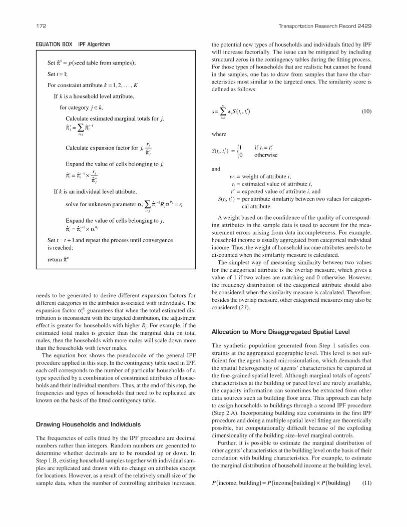
The equation box shows the pseudocode of the general IPF procedure applied in this step. In the contingency table used in IPF, each cell corresponds to the number of particular households of a type specified by a combination of constrained attributes of house-holds and their individual members. Thus, at the end of this step, the frequencies and types of households that need to be replicated are known on the basis of the fitted contingency table.

Drawing households and individuals

The frequencies of cells fitted by the IPF procedure are decimal numbers rather than integers. Random numbers are generated to determine whether decimals are to be rounded up or down. In Step 1.B, existing household samples together with individual sam-ples are replicated and drawn with no change on attributes except for locations. However, as a result of the relatively small size of the sample data, when the number of controlling attributes increases,

the potential new types of households and individuals fitted by IPF will increase factorially. The issue can be mitigated by including structural zeros in the contingency tables during the fitting process. For those types of households that are realistic but cannot be found in the samples, one has to draw from samples that have the char-acteristics most similar to the targeted ones. The similarity score is defined as follows:

s w S t ti i i

i

m

∑ ( )= ′=

, (10)1

where

S(ti, ti′) = t ti i1 if0 otherwise{ = ′

and wi = weight of attribute i, ti = estimated value of attribute i, ti′ = expected value of attribute i, and S(ti, ti′) = per attribute similarity between two values for categori-

cal attribute.

A weight based on the confidence of the quality of correspond-ing attributes in the sample data is used to account for the mea-surement errors arising from data incompleteness. For example, household income is usually aggregated from categorical individual income. Thus, the weight of household income attributes needs to be discounted when the similarity measure is calculated.

The simplest way of measuring similarity between two values for the categorical attribute is the overlap measure, which gives a value of 1 if two values are matching and 0 otherwise. However, the frequency distribution of the categorical attribute should also be considered when the similarity measure is calculated. Therefore, besides the overlap measure, other categorical measures may also be considered (23).

Allocation to More Disaggregated spatial Level

The synthetic population generated from Step 1 satisfies con-straints at the aggregated geographic level. This level is not suf-ficient for the agent-based microsimulation, which demands that the spatial heterogeneity of agents’ characteristics be captured at the fine-grained spatial level. Although marginal totals of agents’ characteristics at the building or parcel level are rarely available, the capacity information can sometimes be extracted from other data sources such as building floor area. This approach can help to assign households to buildings through a second IPF procedure (Step 2.A). Incorporating building size constraints in the first IPF procedure and doing a multiple spatial level fitting are theoretically possible, but computationally difficult because of the exploding dimensionality of the building size–level marginal controls.

Further, it is possible to estimate the marginal distribution of other agents’ characteristics at the building level on the basis of their correlation with building characteristics. For example, to estimate the marginal distribution of household income at the building level,

income, building income building building (11)P P P( )( ) ( )= ×

EqUatIon Box IPF algorithm

p

t

k K

k

j k

j

jr

jr

k

R r

j

t t

j it

i j

j

j

it

it j

j

it

i j

jR

k

it

it R

n

j

j

∑

∑

( )π =

=

=

∈

π = π

π

π = π ×π

α π α =

π = π × α

= +

π

+ −

∈

+

−+

−

∈

−

Set ˆ seed table from samples ;

Set 1;

For constraint attribute 1, 2, . . . ,

If is a household level attribute,

for category ,

Calculate estimated marginal totals for ,ˆ ˆ

Calculate expansion factor for ,ˆ

Expand the value of cells belonging to ,

ˆ ˆˆ

If is an individual level attribute,

solve for unknown parameter , ˆ

Expand the value of cells belonging to ,ˆ ˆ

Set 1 and repeat the process until convergenceis reached;

return ˆ

0

1

1

1

1


According to Equation 11, given the distribution of building char-acteristics, one needs to know only the conditional distribution of household income on buildings. The conditional distribution can be estimated by a discrete choice model drawing on the sample data and available building information. Including estimated marginal distribu-tion of household income in IPF will account for the spatial variation of households’ location choices based on their income and thus generate a more realistic synthetic population (Step 2.B). In Step 2.B, the IPF procedure and the estimation of a conditional distribution of agents’ characteristics are conducted zone by zone to capture the locality.

synTheTiC PoPuLATion GenerATion For sinGAPore

Data sources

The proposed population synthesis approach was applied to gener-ate a synthetic population of 1.29 million households and 3.9 million individuals for 1,092 traffic analysis zones (TAZs) and more than 10,000 residential buildings in Singapore in 2010. The TAZs belong to 55 large planning districts, the level at which marginal data of house-hold and individual characteristics are available from the Singapore Census 2010. For the microdata sample, in the case of Singapore, the Household Interview Travel Survey (HITS) data collected in 2008 by the Land Transport Authority were used. The HITS data col-lected demographic and travel information on 10,840 households and 33,000 individuals, which accounts for about 1% of the total population in Singapore (of citizens and permanent residents).

Although the marginal data from the census are quite spatially aggregated, it was possible to combine these data with other sources to estimate the disaggregated household and individual counts at the individual buildings scale. Postcodes and geographic information system data with building footprints were available from commercial sources (Navteq and GeoPostcodes). Data on housing unit types and capacities were obtained from web services provided by the Housing Development Board. Average property values and the age of buildings were extracted from the REALIS data sets, which record all housing transactions from the late 1990s to 2012. Buildings with missing information on property values and age take information such as price per square meter from nearby buildings in the same real estate development project. The pairing of buildings follows the assumption that buildings having close postcodes and similar addresses belong to the same development project.

selection of Constraint Attributes

The constraint attributes are selected to allow differentiation of agent population attributes that are critical to subsequent behavioral choice models, while also limiting the dimensionality of the fitting procedure to reduce computational effort. Each of the constraint attributes must be available in the sample data set and the census marginal data (Table 1).

evALuATion APProACh

For an understanding of the performance of the approach in this paper under situations in which the sample size is small and mar-ginal data are aggregated, a series of tests are conducted. In this

case, the HITS data set is considered as the known test population and the microdata samples are randomly generated with a sampling rate of 10%. Synthetic populations are generated following the same two-step procedure for all tests. Because of time and space limitations, in the third step the focus is on a single planning district, Ang Mo Kio, one of the older towns outside the central business district of Singapore.

Synthetic population realizations are compared at four differ-ent stages of the procedure to examine how well the marginal distributions of the real population are reproduced. Results are also compared across different spatial levels to test the sensitivity of spatial effect on population allocation. The generated popula-tions are validated against the test population (the HITS data set) at the TAZ level after all of the synthetic households are assigned to buildings. As will be explained later, this test is less than ideal since the 1% HITS sample need not be an accurate representation of the TAZ-level distribution of household attributes. Nevertheless, more disaggregated data are not available, and this approach allows one to compare the spatial pattern produced by this method with that of the 1% sample.

The following are the four stages at which the synthetic population is examined:

1. Pop0. The synthetic population realization produced by fit-ting only household-level constraints. (Constraints on building capacity and number of individuals are ignored, and households are assigned only to those buildings whose postcodes appear in the HITS sample.)

2. Pop1. The synthetic population realization produced by fitting both household- and individual-level constraints at the planning dis-trict level. Constraints on building capacity are ignored, and house-holds are assigned only to those buildings whose postcodes appear in the HITS sample.

3. Pop2.A. The synthetic population realization generated from Step 2.A. Building capacity and household types are constrained when households are allocated to buildings.

4. Pop2.B. The synthetic population generated from Step 2.B. Income distribution constraints are added to the constraints in Step 2.A.

See Figure 1 for the corresponding procedural step generating each type of outcome.

Standardized root mean square error (SRMSE) metrics, defined to measure the divergence of an estimated distribution from the

taBLE 1 Description of Selected Constrained attributes

Attribute Categories

Household size 1, 2, 3, 4, 5, 6+Household incomea <$1,000, $1,000 ∼ $1,999, . . . , >$10,000

Number of workers 0, 1, 2, 3, 4, 5+Dwelling type HDB (2 and 3, 4, 5+), condo and private flat, other

Ethnicity Chinese, Malay, Indian, other

Gender Male, female

Age 0–4, 5–9, 10–19, 20–34, 35–49, 50–64, 65+

Note: Spatial level of constraints for all attributes is 36 planning districts; 55 planning districts were combined to make 36 in the aggregated marginal data provided by Singapore Census (2010). HDB = Housing and Development Board.aCategories = Singapore dollars (S$1 = US $0.679 in 2008).


actual distribution, are used to measure the goodness of fit of the synthetic population realizations (22). SRMSE can be computed as

N

N

i j i j

j

n

i

m

i j

j

n

i

mSRMSE

. . .ˆ

. . .

,..., ,...,

2

11

,...,

11

∑∑

∑∑

( )

( )=

π − π

π==

==

where

N = total number of cells, π̂i,...,j = estimated frequency of cell (i, . . . , j), πi,...,j = corresponding frequency from the real population, and m, n = number of categories for attributes (i, . . . , j).

N is, in the present case, the number of cells specified by joint dis-tribution of attributes (i, . . . , j) included in the results comparison. SRMSE takes the value 0 when the generated population count matches with the real population count in regard to the marginal or joint distribution being tested. The goodness of fit reduces as the SRMSE value increases. However, one issue of the SRMSE mea-sure is that it will increase as N increases even if the count difference does not change. Thus, when SRMSE is applied to measure a sparse high-dimensional matrix, the resultant value is usually high.

In this evaluation stage, the SRMSE value was calculated for the joint distribution of a number of important household and individual attributes, including dwelling type, household income, household size and number of workers, gender, and age groups at the plan-ning district, TAZ, and building levels. The SRMSE value measures the extent to which this paper’s synthesis of the population of Ang Mo Kio results in different spatial-level subtotals that match those observed in the 1% HITS survey. There is considerable variation in the joint distribution of attributes-by-TAZ and attributes-by-buildings observed in this HITS sample, so one would not expect that the synthesis of building populations, constrained only by planning district totals, would match the HITS sample at further disaggregated

spatial levels exactly. The SRMSE results, while less than ideal, pro-vide some indication of how well the Stage 2 methods can account for the fine-grained spatial variability that is evident when detailed building capacity and price information are overlaid with typical travel surveys.

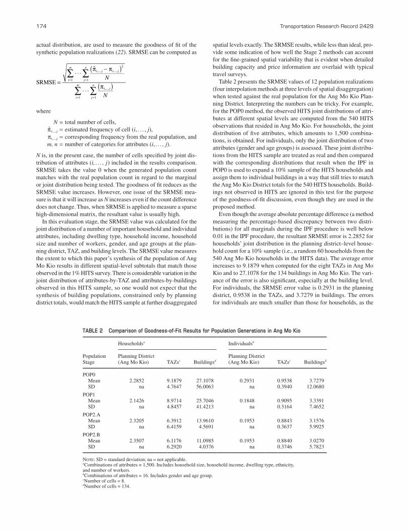
Table 2 presents the SRMSE values of 12 population realizations (four interpolation methods at three levels of spatial disaggregation) when tested against the real population for the Ang Mo Kio Plan-ning District. Interpreting the numbers can be tricky. For example, for the POP0 method, the observed HITS joint distributions of attri-butes at different spatial levels are computed from the 540 HITS observations that resided in Ang Mo Kio. For households, the joint distribution of five attributes, which amounts to 1,500 combina-tions, is obtained. For individuals, only the joint distribution of two attributes (gender and age groups) is assessed. These joint distribu-tions from the HITS sample are treated as real and then compared with the corresponding distributions that result when the IPF in POP0 is used to expand a 10% sample of the HITS households and assign them to individual buildings in a way that still tries to match the Ang Mo Kio District totals for the 540 HITS households. Build-ings not observed in HITS are ignored in this test for the purpose of the goodness-of-fit discussion, even though they are used in the proposed method.

Even though the average absolute percentage difference (a method measuring the percentage-based discrepancy between two distri-butions) for all marginals during the IPF procedure is well below 0.01 in the IPF procedure, the resultant SRMSE error is 2.2852 for households’ joint distribution in the planning district–level house-hold count for a 10% sample (i.e., a random 60 households from the 540 Ang Mo Kio households in the HITS data). The average error increases to 9.1879 when computed for the eight TAZs in Ang Mo Kio and to 27.1078 for the 134 buildings in Ang Mo Kio. The vari-ance of the error is also significant, especially at the building level. For individuals, the SRMSE error value is 0.2931 in the planning district, 0.9538 in the TAZs, and 3.7279 in buildings. The errors for individuals are much smaller than those for households, as the

taBLE 2 Comparison of Goodness-of-Fit Results for Population Generations in ang Mo Kio

Householdsa Individualsb

Population Stage

Planning District(Ang Mo Kio) TAZsc Buildingsd

Planning District(Ang Mo Kio) TAZsc Buildingsd

POP0 Mean 2.2852 9.1879 27.1078 0.2931 0.9538 3.7279 SD na 4.7647 56.0063 na 0.3940 12.0680

POP1 Mean 2.1426 8.9714 25.7046 0.1848 0.9095 3.3391 SD na 4.8457 41.4213 na 0.3164 7.4652

POP2.A Mean 2.3205 6.3912 13.9610 0.1953 0.8843 3.1576 SD na 6.4159 4.5691 na 0.3637 5.9925

POP2.B Mean 2.3507 6.1176 11.0985 0.1953 0.8840 3.0270 SD na 6.2920 4.0376 na 0.3746 5.7823

Note: SD = standard deviation; na = not applicable.aCombinations of attributes = 1,500. Includes household size, household income, dwelling type, ethnicity, and number of workers.bCombinations of attributes = 16. Includes gender and age group.cNumber of cells = 8.dNumber of cells = 134.


SRMSE for households’ joint distribution accounts for the divergence over a much larger size of cells.

A comparison between POP1 and POP0 shows an evident improve-ment of individual joint distribution at the planning-district level (from 0.2931 for POP0 to 0.1848 for POP1), which is expected since POP1 includes individual-level marginal constraints in the Stage 1 IPF while POP0 does not. For individual distribution into TAZs and buildings, the improvement still exists although not as significant in regard to rate.

Because of the thin sample, limited marginals, and vast number of cells, the POP0 and POP1 measures are understandably large, especially at the TAZ and building level. Also, the expected cell counts are small and the randomized rounding (to ensure integers) adds to the SRMSE error. Meanwhile, one can see that when building

capacity and dwelling type are constrained at Stage 3 (POP2.A), the goodness of fit improves not only at the building level but also at the TAZ level. The improvement is more evident for households’ joint distribution, indicating that more of the household characteris-tics are correlated with buildings than with individuals. In addition, the variance of the SRMSE error for households in the buildings decreases significantly. This finding may suggest that the inclusion of building capacity and dwelling type reduces the randomness and arbitrariness of household allocation that may be seen in POP0 and POP1.

Figure 2a shows Singapore, the TAZ boundaries, and the build-ings that housed the 540 households in the HITS sample of Ang Mo Kio. Figure 2, b and c, shows the SRMSE errors at the household and individual levels, respectively, for the POP0 and POP2.B methods.

(a)

(b)

(c)

FIGURE 2 Goodness-of-fit results of test synthetic populations for Ang Mo Kio for crude (POP0) and refined (POP2.B) methods: (a) spatial hierarchical levels of Singapore, (b) goodness of fit for joint distribution of household attributes, and (c) goodness of fit for joint distribution of individual attributes.


In both cases, the errors are fewer and more randomly distributed for the POP2.B results.

The goodness of fit is also improved by including (in POP2.B) the estimated marginal distribution of income as one additional dimension of constraint when households are allocated to buildings. Again, this improvement is more pronounced for households. The discrete choice model used to estimate the marginal income distri-bution of buildings included explanatory variables such as average transaction price, distance to the nearest subway station, and unit type and had an R-squared of about 20%. Nevertheless, the sample 10% of HITS observations is used to fit the discrete choice model, so one is likely to be better off using 100% of the observed HITS data to estimate the POP2.B model for constraining the household income distribution by building when the full population of Ang Mo Kio is allocated.

The test result needs to be interpreted with caution. Because of the small size of the samples in the test compared with the fea-sible combination of controlling attributes, the estimated errors are overstated. Also, the approach contains two IPF procedures. Cor-respondingly, two random rounding procedures need to be conducted to convert decimal frequencies to integer counts. For the micro-simulation seeding, the same procedures are applied to expand the 540 HITS samples in Ang Mo Kio to the full population of that plan-ning district (and likewise for all 36 populated planning districts). Therefore, the full Singapore population synthesis is much less affected by the integer rounding and uses discrete choice models calibrated with much more data for each planning district.

vALiDATion

With building size information obtained from multiple sources and the estimated income distribution conditional on buildings, it was possible to generate the synthetic population at the building level for Singapore. Because the marginal distribution at the building level is not readily available, the estimated household counts at the TAZ level from the Land Transport Authority were used to assess the spatial distribution of the synthetic population results. Out of 1,092 TAZs, household counts of 574 TAZs are less than 5% different from the estimates of the Land Transport Authority. The average absolute per-centage difference between the two data sets is 10.7%. Considering the imperfect building information, nonsynchronous data sources, and the fact that estimates from LTA are also approximated values, the comparison result at the unconstrained TAZ level is acceptable. (Microdata HITS were collected in 2006. Marginal constraints at the planning-district level come from the 2010 SingStat Census. The building information was collected more recently in 2012.) As more reliable and detailed data start to become available for the project, fur-ther validation of the proposed methodology against known marginal or joint distributions at fine-grained spatial levels will be conducted.

ConCLusions

The execution of agent-based microsimulation requires an initial set of agents with detailed socioeconomic and demographic attributes to support the subsequent behavioral models and market models. However, data limitations and privacy reasons restrict the scope and detail with which the entire population can be observed. The objective of the population synthesis procedure is to expand a small microdata sample, by using patterns observed in aggregated data, to

generate a synthetic population that is close to the real population in attribute distributions and correlations that are particularly relevant for the agent behavior that is being simulated. With the development of agent-based microsimulation, the requirement for the accuracy and spatial resolution of synthetic population is increasing. The relation-ships between different types of agents also need to be specified in realistic ways. These requirements make it necessary to consider new data sources and interpolation methods to enable population synthesis at more disaggregated spatial levels.

Recent advances in web-based services, crowdsourcing, and the availability of geographically registered data sets have greatly expanded the amount of relevant, independently available data that can be of assistance in constructing disaggregated synthetic popula-tions. Mining these public and private big-data sources can identify spatial and socioeconomic patterns across households, individuals, jobs, and so forth that can make it practical to construct synthetic populations at the household and building scale. These new data sources can also support urban microsimulation by enriching models with more realistic heterogeneous behaviors and spatial details. However, those readily available data sets are very often not perfect for the research at hand. The barriers include the quality of the data resulting from incompleteness, privacy, cross-referencing difficulties, and other technical issues. Finding ways to enhance the value of tra-ditional surveys and methods through the use of these new data sets and computational techniques is challenging but timely and valuable.

This paper presents a new population synthesis approach aimed at improving the spatially disaggregated accuracy of population gener-ation by using limited microdata and rich, diverse sets of aggregated marginal data. A general IPF method was used to estimate the joint distribution of households’ and individuals’ characteristics under multiple levels of constraints at the level of planning districts for which certain marginal constraints are available. To improve the spa-tial detail of the synthetic population, additional building location, attribute, and occupancy information was collected from multiple sources and used to constrain housing locations by using a second IPF pro cedure that addresses building capacity as well as spatio-demographic patterns estimated by using a discrete choice model. The procedure yields realistic spatial heterogeneity while preserving some of the joint distribution of household and locational charac-teristics. As the test results show, the proposed two-step IPF-based approach does yield better fits at more fine-grained but unconstrained spatial levels than do traditional population synthesis methods. This research represents one of the efforts to find practical methods and algorithms to combine new data sources with traditional data sources to piece together the knowledge about entire populations in ways that preserve much of the spatial and attribute interactions.

ACknoWLeDGMenTs

This research is part of the SimMobility project funded by the Singapore National Research Foundation through the Singapore–MIT Alliance for Research and Technology Center for Future Mobility. The authors are grateful for valuable inputs from Moshe Ben-Akiva. The authors also acknowledge the contributions of other collaborators at MIT and in the Future Mobility team including Chris Zegras, Mi Diao, Xiaosu Ma, and Pedro J. S. Gandol. In addition, the authors appreciate the support of the Singapore Urban Redevelopment Authority and Singapore Land Transport Authority on the collec-tion of the HITS data set, the REALIS data set, and other helpful information.


reFerenCes

1. Balmer, M., M. Rieser, K. Meister, D. Charypar, N. Lefebvre, K. Nagel, and K. Axhausen. MATSim-T: Architecture and Simulation Times. In Multi-Agent Systems for Traffic and Transportation Engineering (A. L. C. Bazzan and F. Klügl, eds.), 2009, Information Science Reference, Hershey, Penn., pp. 57–78.

2. Ben-Akiva, M., H. N. Koutsopoulos, C. Antoniou, and R. Balakrishna. Traffic Simulation with DynaMIT. In Fundamentals of Traffic Simulation, Springer, New York, 2010, pp. 363–398.

3. Waddell, P. UrbanSim: Modeling Urban Development for Land Use, Transportation, and Environmental Planning. Journal of the American Planning Association, Vol. 68, No. 3, 2002, pp. 297–314.

4. Salvini, P. A., and E. J. Miller. ILUTE: An Operational Prototype of a Comprehensive Microsimulation Model of Urban Systems. Networks and Spatial Economics, Vol. 5, No. 2, 2005, pp. 217–234.

5. Wagner, P., and M. Wegener. Urban Land Use, Transport, and Environ-ment Models: Experiences with an Integrated Microscopic Approach. The Planning Review, Vol. 170, No. 3, 2007, pp. 45–56.

6. Martínez, F., and P. Donoso. The MUSSA II Land Use Auction Equilib-rium Model. In Residential Location Choice, Springer, Berlin Heidelberg, 2010, pp. 99–113.

7. Beckman, J. R., K. A. Baggerly, and M. D. McKay. Creating Synthetic Baseline Populations. Transportation Research Part A, Vol. 30, No. 6, 1996, pp. 415–429.

8. Deming, W. E., and F. F. Stephan. On the Least Squares Adjustment of a Sampled Frequency Table When the Expected Marginal Totals Are Known. Annals of Mathematical Statistics, Vol. 11, No. 4, 1940, pp. 427–444.

9. Stephan, F. An Iterative Method of Adjusting Sample Frequency Tables When Expected Marginal Totals Are Known. Annals of Mathematical Statistics, Vol. 13, No. 2, 1942, pp. 166–178.

10. Fienberg, S. E. An Iterative Procedure for Estimation in Contingency Tables. Annals of Mathematical Statistics, Vol. 41, No. 3, 1970, pp. 907–917.

11. Ireland, C. T., and S. Kullback. Contingency Tables with Given Marginals. Biometrika, Vol. 55, No. 1, 1968, pp. 179–188.

12. Arentze, T., H. J. P. Timmermans, and F. Hofman. Creating Synthetic Household Populations: Problems and Approach. In Transportation Research Record: Journal of the Transportation Research Board, No. 2014, Transportation Research Board of the National Academies, Wash-ington, D.C., 2007, pp. 85–91.

13. Auld, J., and A. Mohammadian. Efficient Methodology for Generating Synthetic Populations with Multiple Control Levels. In Transporta-tion Research Record: Journal of the Transportation Research Board, No. 2175, Transportation Research Board of the National Academies, Washington, D.C., 2010, pp. 138–147.

14. Rich, J., and I. Mulalic. Generating Synthetic Baseline Populations from Register Data. Transportation Research Part A, Vol. 46, No. 3, 2012, pp. 467–479.

15. Smith, D. M., G. P. Clarke, and K. Harland. Improving the Synthetic Data Generation Process in Spatial Microsimulation Models. Environment and Planning A, Vol. 41, No. 5, 2009, p. 1251.

16. Guo, J. Y., and C. R. Bhat. Population Synthesis for Microsimulating Travel Behavior. In Transportation Research Record: Journal of the Transportation Research Board, No. 2014, Transportation Research Board of the National Academies, Washington, D.C., 2007, pp. 92–101.

17. Pritchard, D. R., and E. J. Miller. Advances in Population Synthesis: Fitting Many Attributes per Agent and Fitting to Household and Person Margins Simultaneously. Transportation, Vol. 39, No. 3, 2012, pp. 685–704.

18. Ye, X., K. C. Konduri, R. M. Pendyala, B. Sana, and P. Waddell. Methodol-ogy to Match Distributions of Both Household and Person Attributes in the Generation of Synthetic Populations. Presented at 88th Annual Meeting of the Transportation Research Board, Washington, D.C., 2009.

19. Müller, K., and K. W. Axhausen. Hierarchical IPF: Generating a Syn-thetic Population for Switzerland. Eidgenössische Technische Hochschule Zürich, Institution for Transport Planning and Systems, Zurich, Switzer-land, 2011.

20. Barthelemy, J., and P. L. Toint. Synthetic Population Generation Without a Sample. Transportation Science, Vol. 47, No. 2, 2013, pp. 266–279.

21. Farooq, B., M. Bierlaire, R. Hurtubia, and G. Flötteröd. Simulation Based Population Synthesis. Transportation Research Part B, Vol. 58, 2013, pp. 243–263.

22. Ordóñez Medina, S. A., and A. Erath. Estimating Dynamic Workplace Capacities Using Public Transport Smart Card Data and Household Travel Survey in Singapore. Presented at 92nd Annual Meeting of the Transportation Research Board, Washington, D.C., 2013.

23. Boriah, S., V. Chandola, and V. Kumar. Similarity Measures for Cate-gorical Data: A Comparative Evaluation. Proc., 2008 SIAM International Conference on Data Mining (R. Sedgewick and W. Szpankowski, eds.), Society for Industrial and Applied Mathematics, Philadelphia, Penn., 2008, pp. 243–254.

The Transportation Demand Forecasting Committee peer-reviewed this paper.

synthetic population generation at disaggregated...

Documents