synthesizing designs with inter-part dependencies...

Proceedings of the ASME 2018 International Design Engineering Technical Conferences &Computers and Information in Engineering Conference

IDETC/CIE 2018August 26-29, 2018, Quebec City, Quebec, Canada

DETC2018-85339

SYNTHESIZING DESIGNS WITH INTER-PART DEPENDENCIES USINGHIERARCHICAL GENERATIVE ADVERSARIAL NETWORKS

Wei Chen∗Dept. of Mechanical Engineering

University of MarylandCollege Park, Maryland 20742Email: [email protected]

Ashwin JeyaseelanDept. of Computer Science

University of MarylandCollege Park, Maryland 20742Email: [email protected]

Mark FugeDept. of Mechanical Engineering

University of MarylandCollege Park, Maryland 20742

Email: [email protected]

ABSTRACTReal-world designs usually consist of parts with hierarchi-

cal dependencies, i.e., the geometry of one component (a childshape) is dependent on another (a parent shape). We propose amethod for synthesizing this type of design. It decomposes theproblem of synthesizing the whole design into synthesizing eachcomponent separately but keeping the inter-component depen-dencies satisfied. This method constructs a two-level generativeadversarial network to train two generative models for parentand child shapes, respectively. We then use the trained gener-ative models to synthesize or explore parent and child shapesseparately via a parent latent representation and infinite childlatent representations, each conditioned on a parent shape. Weevaluate and discuss the disentanglement and consistency of la-tent representations obtained by this method. We show thatshapes change consistently along any direction in the latentspace. This property is desirable for design exploration over thelatent space.

INTRODUCTIONRepresenting a high-dimensional design space with a lower-

dimensional latent space makes it easier to explore, visualize, oroptimize complex designs. This often means finding a latent rep-resentation, or a manifold, along which valid design geometriesmorph [1, 2].

While this works well for single parts, designs usually have

∗Address all correspondence to this author.

hierarchical structures. For example, the size and position of a(conduit, lightening, or alignment) hole in an airfoil depend onthe shape of the airfoil, thus there is a hierarchical relationshipbetween the airfoil and the hole in it. Here the airfoil is called theparent shape, and the hole is called the child shape. In this case,one may want to identify first the parent manifold that capturesmajor variation of parent shapes, and then the child manifold thatcaptures major variation of feasible child shapes conditioned onany parent shape (Fig. 1). Because, for example, we may first op-timize the airfoil shape on the airfoil manifold (parent) to obtainthe optimal lift and drag; and then given the optimal airfoil, wemay optimize the hole’s size and position on the hole manifold(child) for other consideration.

However, finding individual part manifolds that both repre-sent the design space well, while also satisfying part configura-tion, is non-trivial. To learn the inter-part dependency, one candefine explicit constraints [3, 4] or learn implicit constraints viaadaptive sampling [2,5]. The former uses hard-coded constraintsand hence lacks flexibility; whereas the latter queries externalsources by human annotation, experiment, or simulation, thusis expensive. In this paper, we solve the problem by identify-ing different levels of manifolds, where the higher-level mani-fold imposes implicit constraints on the lower-level manifolds.Our main contribution is a deep generative model that synthe-sizes designs in a hierarchical manner: it first synthesizes theparent shape, and then the child shape conditioned on its par-ent. The model simultaneously captures a parent manifold andinfinite child manifolds which are conditioned on parent shapes.

1 Copyright c© 2018 by ASME

Figure 1: MANIFOLDS OF PARENT AND CHILD SHAPES.

This results in two latent spaces allowing synthesis and searchingof parent and child shapes. Our method is fully data-driven andrequires no hard-coded rules, querying external sources, or com-plex preprocessing [6], except for specifying parent and childshapes in the dataset.

RELATED WORKOur work produces generative models that synthesize de-

signs from latent representations. There are primarily twostreams of related research—design space dimensionality reduc-tion and design synthesis—from the fields of engineering designand computer graphics. We also review generative adversarialnets (GAN) [7], which we use to build our model.

Design Space Dimensionality ReductionWhile designs can be parametrized by various tech-

niques [8], the number of design variables (i.e., the dimension-ality of a design space) increases with the geometric variabilityof designs. In tasks like design optimization, to find better de-signs we usually need a design space with higher variability, i.e.,higher dimensionality. This demand brings up the problem ofexploring a high-dimensional design space. Based on the curseof dimensionality [9], the cost of exploring the design spacegrows exponentially with its dimensionality. Thus researchershave studied approaches of reducing the design space dimen-sionality. Normally, dimensionality reduction methods identify alower-dimensional latent space that captures most of the designspace’s variability. This can be grouped into linear and non-linearmethods.

Linear dimensionality reduction methods select a set of opti-mal directions or basis functions where the variance of shape ge-ometry or certain simulation output is maximized. Such methodsincludes the Karhunen-Loeve expansion (KLE) [10, 11], princi-pal component analysis (PCA) [12], and the active subspaces ap-proach [13].

In practice, it is more reasonable to assume that design vari-ables lie on a non-linear manifold, rather than a hyperplane. Thusresearchers also apply non-linear methods to reduce the dimen-sionality of design spaces. This non-linearity can be achievedby 1) applying linear reduction techniques locally to constructa non-linear global manifold [14, 15, 16, 17, 12]; 2) using ker-nel methods with linear reduction techniques [1, 12]; 3) la-tent variable models like Gaussian process latent variable model(GPLVM) and generative topographic mapping (GTM) [18]; and4) neural networks based approaches such as self-organizingmaps [19] and autoencoders [20, 1, 12, 21].

This work differs from these approaches in that we aimat identifying two-level latent spaces with the lower-level en-codes inter-part dependencies, rather than learning only one la-tent space for the complete design.

Data-Driven Design SynthesisDesign synthesis methods can be divided into two cate-

gories: rule-based and data-driven design synthesis. The former(e.g., grammars-based design synthesis [22, 4, 3]) requires label-ing of the reference points or surfaces and defining rule sets, sothat new designs are synthesized according to this hard-codedprior knowledge; while the latter learns rules/constraints from adatabase and generates plausible new designs with similar struc-ture/function to exemplars in the database.

Usually dimensionality reduction techniques allow inversetransformations from the latent space back to the design space,thus can synthesize new designs from latent variables [11, 1, 12,21]. For example, under the PCA model, the latent variables de-fine a linear combination of principal components to synthesizea new design [11]; for local manifold based approaches, a newdesign can be synthesized via interpolation between neighbor-ing points on the local manifold [17]; and under the autoencodermodel, the trained decoder maps any given point in the latentspace to a new design [20, 21].

Methods for synthesizing 3D models are frequently stud-ied by the field of computer graphics. Generally, researchershave employed generative models such as kernel density esti-mation [23], Boltzmann machines [24], variational autoencoders(VAEs) [25], and generative adversarial nets (GANs) [26, 27] tolearn the distribution of samples in the design space, and synthe-size new designs by drawing samples from the learned distribu-tion. Discriminative models like deep residual networks [28] arealso used to generate 3D shapes.

There are also methods that synthesize new shapes by as-


sembling or reorganizing parts from an existing shape database,while preserving the desired structures [29, 6, 30, 31, 32]. Theshapes are usually parameterized by high-level abstract represen-tations, such as hand-crafted feature vectors [6] or shape gram-mars [30]. While these methods edit shapes at a high-level, theydo not control the local geometry of each synthesized compo-nent.

Previously the inter-part dependencies of shapes have beenmodeled by grammar induction [30], kernel density estima-tion [33], probabilistic graph models [29,6,24], and recursive au-toencoders [27]. Those methods handle part relations and designsynthesis separately. In contrast, our method encodes part rela-tions through the model architecture, so that it simultaneouslylearns the inter-part dependencies and single part geometry vari-ation. The model can also be used for inferring the generativedistribution of child shapes conditioned on any parent shape.

Generative Adversarial NetworksGenerative adversarial nets [7] model a game between a gen-

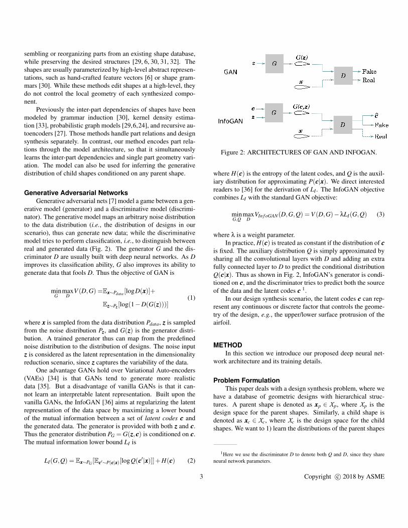
erative model (generator) and a discriminative model (discrimi-nator). The generative model maps an arbitrary noise distributionto the data distribution (i.e., the distribution of designs in ourscenario), thus can generate new data; while the discriminativemodel tries to perform classification, i.e., to distinguish betweenreal and generated data (Fig. 2). The generator G and the dis-criminator D are usually built with deep neural networks. As Dimproves its classification ability, G also improves its ability togenerate data that fools D. Thus the objective of GAN is

minG

maxD

V (D,G) =Exxx∼Pdata [logD(xxx)]+

Ezzz∼Pzzz [log(1−D(G(zzz)))](1)

where xxx is sampled from the data distribution Pdata, zzz is sampledfrom the noise distribution Pzzz, and G(zzz) is the generator distri-bution. A trained generator thus can map from the predefinednoise distribution to the distribution of designs. The noise inputzzz is considered as the latent representation in the dimensionalityreduction scenario, since zzz captures the variability of the data.

One advantage GANs hold over Variational Auto-encoders(VAEs) [34] is that GANs tend to generate more realisticdata [35]. But a disadvantage of vanilla GANs is that it can-not learn an interpretable latent representation. Built upon thevanilla GANs, the InfoGAN [36] aims at regularizing the latentrepresentation of the data space by maximizing a lower boundof the mutual information between a set of latent codes ccc andthe generated data. The generator is provided with both zzz and ccc.Thus the generator distribution PG = G(zzz,ccc) is conditioned on ccc.The mutual information lower bound LI is

LI(G,Q) = Exxx∼PG [Eccc′∼P(ccc|xxx)[logQ(ccc′|xxx)]]+H(ccc) (2)

z

Figure 2: ARCHITECTURES OF GAN AND INFOGAN.

where H(ccc) is the entropy of the latent codes, and Q is the auxil-iary distribution for approximating P(ccc|xxx). We direct interestedreaders to [36] for the derivation of LI . The InfoGAN objectivecombines LI with the standard GAN objective:

minG,Q

maxD

VIn f oGAN(D,G,Q) =V (D,G)−λLI(G,Q) (3)

where λ is a weight parameter.In practice, H(ccc) is treated as constant if the distribution of ccc

is fixed. The auxiliary distribution Q is simply approximated bysharing all the convolutional layers with D and adding an extrafully connected layer to D to predict the conditional distributionQ(ccc|xxx). Thus as shown in Fig. 2, InfoGAN’s generator is condi-tioned on ccc, and the discriminator tries to predict both the sourceof the data and the latent codes ccc 1.

In our design synthesis scenario, the latent codes ccc can rep-resent any continuous or discrete factor that controls the geome-try of the design, e.g., the upper/lower surface protrusion of theairfoil.

METHODIn this section we introduce our proposed deep neural net-

work architecture and its training details.

Problem FormulationThis paper deals with a design synthesis problem, where we

have a database of geometric designs with hierarchical struc-tures. A parent shape is denoted as xxxp ∈ Xp, where Xp is thedesign space for the parent shapes. Similarly, a child shape isdenoted as xxxc ∈ Xc, where Xc is the design space for the childshapes. We want to 1) learn the distributions of the parent shapes

1Here we use the discriminator D to denote both Q and D, since they shareneural network parameters.


zp

cp

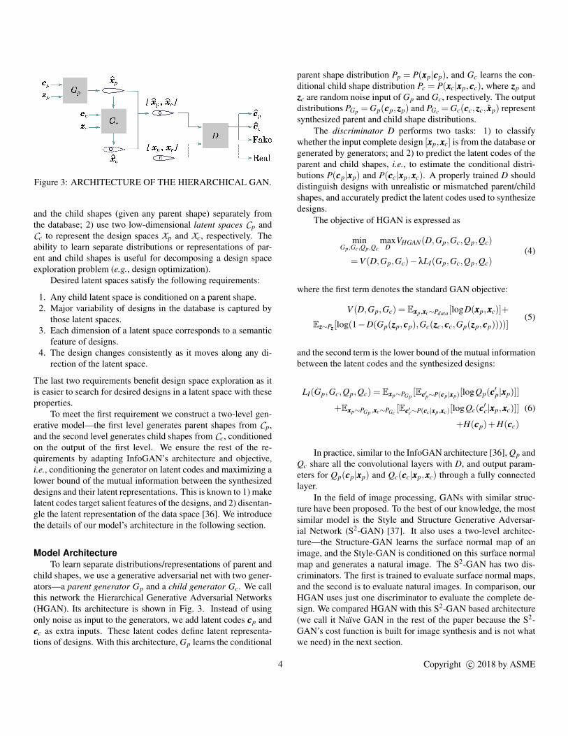
Figure 3: ARCHITECTURE OF THE HIERARCHICAL GAN.

and the child shapes (given any parent shape) separately fromthe database; 2) use two low-dimensional latent spaces Cp andCc to represent the design spaces Xp and Xc, respectively. Theability to learn separate distributions or representations of par-ent and child shapes is useful for decomposing a design spaceexploration problem (e.g., design optimization).

Desired latent spaces satisfy the following requirements:

1. Any child latent space is conditioned on a parent shape.2. Major variability of designs in the database is captured by

those latent spaces.3. Each dimension of a latent space corresponds to a semantic

feature of designs.4. The design changes consistently as it moves along any di-

rection of the latent space.

The last two requirements benefit design space exploration as itis easier to search for desired designs in a latent space with theseproperties.

To meet the first requirement we construct a two-level gen-erative model—the first level generates parent shapes from Cp,and the second level generates child shapes from Cc, conditionedon the output of the first level. We ensure the rest of the re-quirements by adapting InfoGAN’s architecture and objective,i.e., conditioning the generator on latent codes and maximizing alower bound of the mutual information between the synthesizeddesigns and their latent representations. This is known to 1) makelatent codes target salient features of the designs, and 2) disentan-gle the latent representation of the data space [36]. We introducethe details of our model’s architecture in the following section.

Model ArchitectureTo learn separate distributions/representations of parent and

child shapes, we use a generative adversarial net with two gener-ators—a parent generator Gp and a child generator Gc. We callthis network the Hierarchical Generative Adversarial Networks(HGAN). Its architecture is shown in Fig. 3. Instead of usingonly noise as input to the generators, we add latent codes cccp andcccc as extra inputs. These latent codes define latent representa-tions of designs. With this architecture, Gp learns the conditional

parent shape distribution Pp = P(xxxp|cccp), and Gc learns the con-ditional child shape distribution Pc = P(xxxc|xxxp,cccc), where zzzp andzzzc are random noise input of Gp and Gc, respectively. The outputdistributions PGp = Gp(cccp,zzzp) and PGc = Gc(cccc,zzzc, xxxp) representsynthesized parent and child shape distributions.

The discriminator D performs two tasks: 1) to classifywhether the input complete design [xxxp,xxxc] is from the database orgenerated by generators; and 2) to predict the latent codes of theparent and child shapes, i.e., to estimate the conditional distri-butions P(cccp|xxxp) and P(cccc|xxxp,xxxc). A properly trained D shoulddistinguish designs with unrealistic or mismatched parent/childshapes, and accurately predict the latent codes used to synthesizedesigns.

The objective of HGAN is expressed as

minGp,Gc,Qp,Qc

maxD

VHGAN(D,Gp,Gc,Qp,Qc)

=V (D,Gp,Gc)−λLI(Gp,Gc,Qp,Qc)(4)

where the first term denotes the standard GAN objective:

V (D,Gp,Gc) = Exxxp,xxxc∼Pdata [logD(xxxp,xxxc)]+

Ezzz∼Pzzz [log(1−D(Gp(zzzp,cccp),Gc(zzzc,cccc,Gp(zzzp,cccp))))](5)

and the second term is the lower bound of the mutual informationbetween the latent codes and the synthesized designs:

LI(Gp,Gc,Qp,Qc) = Exxxp∼PGp[Eccc′p∼P(cccp|xxxp)[logQp(ccc′p|xxxp)]]

+Exxxp∼PGp ,xxxc∼PGc[Eccc′c∼P(cccc|xxxp,xxxc)[logQc(ccc′c|xxxp,xxxc)]]

+H(cccp)+H(cccc)

(6)

In practice, similar to the InfoGAN architecture [36], Qp andQc share all the convolutional layers with D, and output param-eters for Qp(cccp|xxxp) and Qc(cccc|xxxp,xxxc) through a fully connectedlayer.

In the field of image processing, GANs with similar struc-ture have been proposed. To the best of our knowledge, the mostsimilar model is the Style and Structure Generative Adversar-ial Network (S2-GAN) [37]. It also uses a two-level architec-ture—the Structure-GAN learns the surface normal map of animage, and the Style-GAN is conditioned on this surface normalmap and generates a natural image. The S2-GAN has two dis-criminators. The first is trained to evaluate surface normal maps,and the second is to evaluate natural images. In comparison, ourHGAN uses just one discriminator to evaluate the complete de-sign. We compared HGAN with this S2-GAN based architecture(we call it Naıve GAN in the rest of the paper because the S2-GAN’s cost function is built for image synthesis and is not whatwe need) in the next section.


EXPERIMENTSWe train HGAN on two datasets, and evaluate the trained

generative models through quantitative measures.

Experimental SetupDataset. We denote the two datasets as A+H (airfoils

with holes) and S+E (superformulas [38] with ellipses). Bothdatasets have over 90,000 samples. Examples of the two datasetsare shown in Fig. 4.

The airfoil shapes are from the UIUC airfoil coordinatesdatabase2, which provides the Cartesian coordinates for nearly1,600 airfoils. Each airfoil is represented with 100 Cartesian co-ordinates, resulting in a 100× 2 matrix. We use these airfoilsas parent shapes. For each airfoil we add a hole (e.g., a conduithole) as its child shape. We add the holes by generating circleswith random centers and sizes, and ruling out the ones not insidethe airfoils. Each hole is also represented with 100 Cartesian co-ordinates. Hence each sample in this A+H dataset is a 200× 2matrix.

Though targeted for real-world applications, the airfoils maynot be a perfect experimental dataset to visualize the latentspace, because the ground truth intrinsic dimension3 of the airfoildataset is unknown. Thus we create another dataset using super-formulas and ellipses, the intrinsic dimensions of which are con-trollable. The superformula is a generalization of the ellipse [38].We generate superformulas as parent shapes using the followingequations:

n1 = 10s1

n2 = n3 = 10(s1 + s2)

r(θ) = (|cosθ|n2 + |sinθ|n3)− 1

n1

(x,y) = (r(θ)cosθ,r(θ)sinθ)

(7)

where s1,s2 ∈ [0,1], and (x,y) is a Cartesian coordinate. Foreach superformula, we sample 100 evenly spaced θ from 0 to2π, and get 100 grid-point Cartesian coordinates. Equations (7)show that we can control the deformation of the superformulashape with s1 and s2. Thus the ground truth intrinsic dimen-sion of our superformula dataset is two. We use ellipses as childshapes. We generate ellipses with random semi-major axis andsemi-minor axis lengths and fixed centers (at the centers of the el-lipses). Hence the intrinsic dimension for the ellipses is also two.We rule out the ellipses that are not inside the superformulas. Weset the intrinsic dimensions of both superformulas and ellipses totwo because we want a two-dimensional latent space which is

2http://m-selig.ae.illinois.edu/ads/coord_database.html

3The intrinsic dimension is the minimum number of variables required to rep-resent the data.

easy to visualize, evaluate, and verify. As with the A+H dataset,every superformula/ellipse is represented with 100 Cartesian co-ordinates, thus each sample in the S+E dataset is also a 200× 2matrix.

Network Details. Figure 5 shows the details of the dis-criminator. The input is a 200× 2 matrix, containing the parentshape and the child shape, each of which is expressed with 1002D Cartesian coordinates. The input goes through four down-sampling blocks, each performs a 1D convolution, a batch nor-malization, and a LeakyReLU activation. The length of each 1Dconvolution window is 5. The last downsampling block is fol-lowed by fully connected layers, predicting the mean and logstandard deviation of latent codes, and the source of the input.

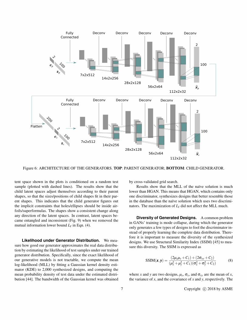
The generators’ architectures, as shown in Fig. 6, basicallymirror that of the discriminator. The parent generator gets two in-puts: the parent latent codes cccp of size 2 and the input noise zzzp ofsize 100. The inputs are then concatenated, fed into a fully con-nected layer, and reshaped to a 3D matrix. Then it goes throughfour upsampling blocks. The difference between the downsam-pling block and the upsampling block is that we use deconvolu-tion (also called transposed convolution) [39] in the upsamplingblock, rather than convolution in the downsampling block. Thefinal layer is a deconvolutional layer with hyperbolic tangent ac-tivation, and outputs the parent shape xxxp, a 2×100×1 matrix. Itis then flattened and fed into the child generator. The child gen-erator has the same architecture as the parent generator, exceptthat there are three inputs—the flattened parent shape xxxp of size200, the child latent codes cccc of size 2 and the input noise zzzc ofsize 100. The final output is the child shape xxxc.

We compared HGAN with a naıve solution where we builttwo independent GANs—one for generating parent shapes, andanother for generating child shapes conditioned on parent shapes.So there are two generators and two discriminators in this naıvesolution. One discriminator for predicting the source of parentshapes and parent latent codes, and the other for predicting thesource of child shapes and child latent codes. We used the samearchitecture for both generators as in HGAN.

Training Details. At training, we sample cccp and cccc fromuniform distribution U(0,1), and zzzp and zzzc from normal distri-bution N (0,0.25). The hyperparameter λ in Eqn. (4) was set to 1in all experiments. The network was optimized using Adam [40]with the momentum terms β1 = 0.5 and β2 = 0.999. The learningrates of the discriminator and two generators were set to 0.00005and 0.0002, respectively. The total number of training steps was100,000. The batch size was 100. The training procedure is sum-marized in Algorithm 1.

To avoid the problem that the generative distribution andthe true data distribution does not have overlapping support, weadded normally distributed instance noise to discriminator in-


http://m-selig.ae.illinois.edu/ads/coord_database.html

http://m-selig.ae.illinois.edu/ads/coord_database.html

Figure 4: RANDOMLY SELECTED TRAINING DATA. LEFT: SUPERFORMULAS WITH ELLIPSES; RIGHT: AIRFOILS WITHHOLES.

2

200...

100x1x64

...

50x1x128

...

25x1x256

...

13x1x512

1024

Real/Fake

128

128

log σ (cp)

µ (cp)

log σ (cc)

µ (cc)

[ xp , xc ]

Fully

Connected

Convolution Convolution

ConvolutionConvolution Fully

Connected

Figure 5: ARCHITECTURE OF THE DISCRIMINATOR.

puts [41]. Its standard deviation decreases as the number of train-ing steps increases:

σ = e−t/10000

We used Keras [42] with TensorFlow [43] backend to buildthe networks. We trained our networks on a Nvidia Titan X GPU.For each experiment, the training process took around 6.5 hours,and the testing took less than 10 seconds.

Results and DiscussionWe evaluated the performance of our trained generative

models using both visual inspection and quantitative measures.The quantitative results are shown in Table 1.

Visual Inspection. The captured latent spaces for bothexamples are shown in Fig. 7 and Fig. 8. To test the general-ization ability of the child generator, we use parent shapes fromthe test set as inputs to the child generator. Thus each child la-


100

2...

7x2x512

...

14x2x256

...

28x2x128

...

56x2x64

...

112x2x32

2

100

xp

cp

zp

100

2...

7x2x512

...

14x2x256

...

28x2x128

...

56x2x64

...

112x2x32

2

100

xc

cc

zc

200

Flatten

Fully

Connected

Deconv Deconv Deconv Deconv Deconv

Fully

Connected

Deconv Deconv Deconv Deconv Deconv

Figure 6: ARCHITECTURE OF THE GENERATORS. TOP: PARENT GENERATOR; BOTTOM: CHILD GENERATOR.

tent space shown in the plots is conditioned on a random testsample (plotted with dashed lines). The results show that thechild latent spaces adjust themselves according to their parentshapes, so that the sizes/positions of child shapes fit in their par-ent shapes. This indicates that the child generator figures outthe implicit constraints that holes/ellipses should be inside air-foils/superformulas. The shapes show a consistent change alongany direction of the latent spaces. In contrast, latent spaces be-came entangled and inconsistent (Fig. 9) when we removed themutual information lower bound LI in Eqn. (4).

Likelihood under Generator Distribution. We mea-sure how good our generator approximates the real data distribu-tion by estimating the likelihood of test samples under our trainedgenerator distribution. Specifically, since the exact likelihood ofour generative models is not tractable, we compute the meanlog-likelihood (MLL) by fitting a Gaussian kernel density esti-mator (KDE) to 2,000 synthesized designs, and computing themean probability density of test data under the estimated distri-bution [44]. The bandwidth of the Gaussian kernel was obtained

by cross-validated grid search.Results show that the MLL of the naıve solution is much

lower than HGAN. This means that HGAN, which contains onlyone discriminator, synthesizes designs that better resemble thosein the database than the naıve solution which uses two discrimi-nators. The maximization of LI did not affect the MLL much.

Diversity of Generated Designs. A common problemin GANs’ training is mode collapse, during which the generatoronly generates a few types of designs to fool the discriminator in-stead of properly learning the complete data distribution. There-fore it is important to measure the diversity of the synthesizeddesigns. We use Structural Similarity Index (SSIM) [45] to mea-sure this diversity. The SSIM is expressed as

SSIM(xxx,yyy) =(2µxµy +C1)+(2σxy +C2)

(µ2x +µ2

y +C1)(σ2x +σ2

y +C2)(8)

where x and y are two designs, µx, σx, and σxy are the mean of x,the variance of x, and the covariance of x and y, respectively. The


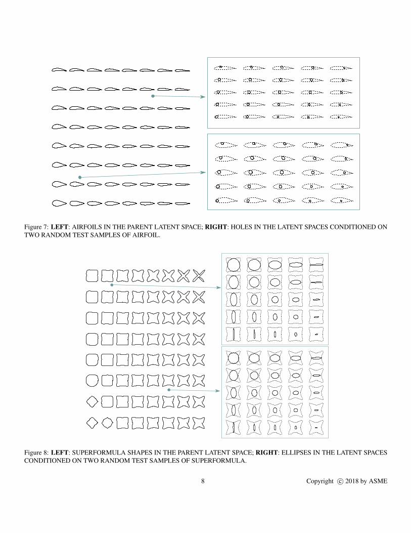
Figure 7: LEFT: AIRFOILS IN THE PARENT LATENT SPACE; RIGHT: HOLES IN THE LATENT SPACES CONDITIONED ONTWO RANDOM TEST SAMPLES OF AIRFOIL.

Figure 8: LEFT: SUPERFORMULA SHAPES IN THE PARENT LATENT SPACE; RIGHT: ELLIPSES IN THE LATENT SPACESCONDITIONED ON TWO RANDOM TEST SAMPLES OF SUPERFORMULA.


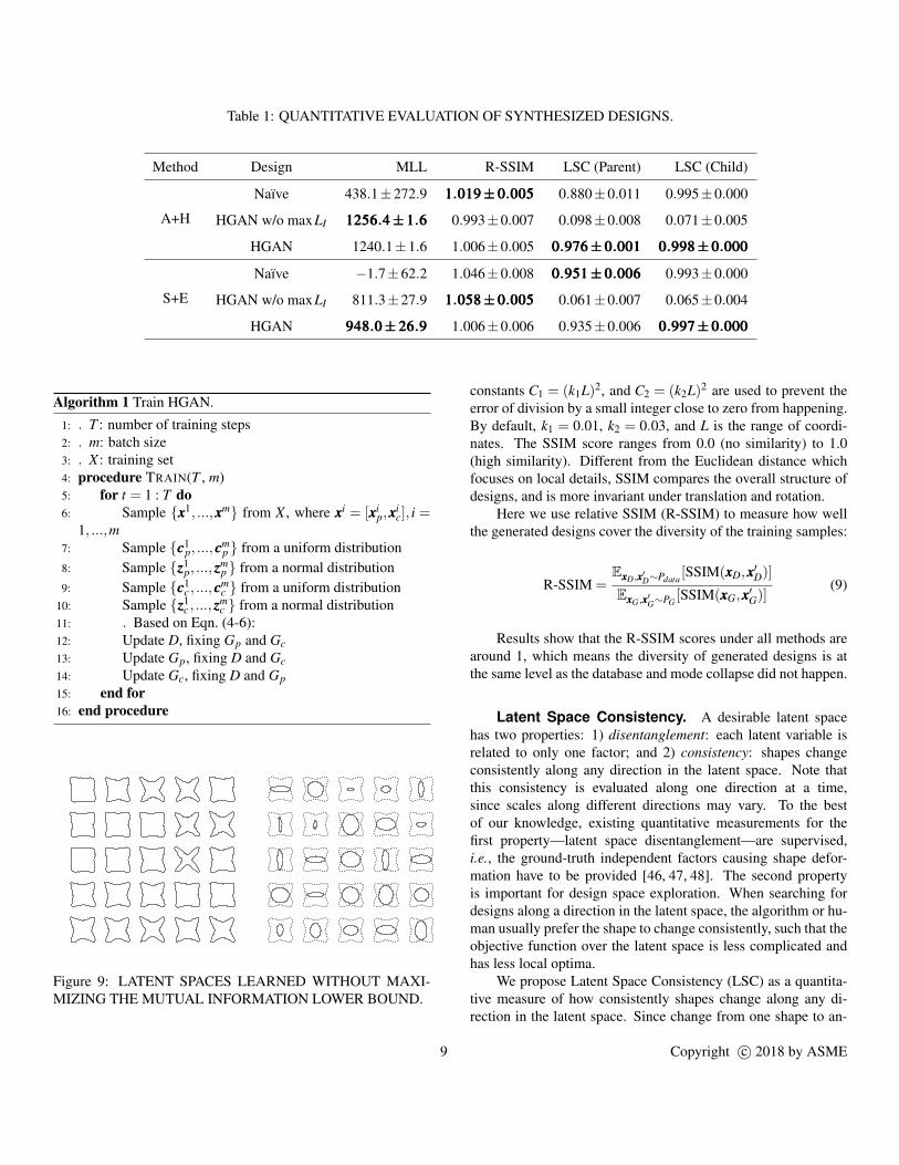
Table 1: QUANTITATIVE EVALUATION OF SYNTHESIZED DESIGNS.

Method Design MLL R-SSIM LSC (Parent) LSC (Child)

A+H

Naıve 438.1±272.9 111...000111999±±±000...000000555 0.880±0.011 0.995±0.000

HGAN w/o maxLI 111222555666...444±±±111...666 0.993±0.007 0.098±0.008 0.071±0.005

HGAN 1240.1±1.6 1.006±0.005 000...999777666±±±000...000000111 000...999999888±±±000...000000000

S+E

Naıve −1.7±62.2 1.046±0.008 000...999555111±±±000...000000666 0.993±0.000

HGAN w/o maxLI 811.3±27.9 111...000555888±±±000...000000555 0.061±0.007 0.065±0.004

HGAN 999444888...000±±±222666...999 1.006±0.006 0.935±0.006 000...999999777±±±000...000000000

Algorithm 1 Train HGAN.

1: . T : number of training steps2: . m: batch size3: . X : training set4: procedure TRAIN(T , m)5: for t = 1 : T do6: Sample {xxx1, ...,xxxm} from X , where xxxi = [xxxi

p,xxxic], i =

1, ...,m7: Sample {ccc1

p, ...,cccmp } from a uniform distribution

8: Sample {zzz1p, ...,zzz

mp } from a normal distribution

9: Sample {ccc1c , ...,ccc

mc } from a uniform distribution

10: Sample {zzz1c , ...,zzz

mc } from a normal distribution

11: . Based on Eqn. (4-6):12: Update D, fixing Gp and Gc13: Update Gp, fixing D and Gc14: Update Gc, fixing D and Gp15: end for16: end procedure

Figure 9: LATENT SPACES LEARNED WITHOUT MAXI-MIZING THE MUTUAL INFORMATION LOWER BOUND.

constants C1 = (k1L)2, and C2 = (k2L)2 are used to prevent theerror of division by a small integer close to zero from happening.By default, k1 = 0.01, k2 = 0.03, and L is the range of coordi-nates. The SSIM score ranges from 0.0 (no similarity) to 1.0(high similarity). Different from the Euclidean distance whichfocuses on local details, SSIM compares the overall structure ofdesigns, and is more invariant under translation and rotation.

Here we use relative SSIM (R-SSIM) to measure how wellthe generated designs cover the diversity of the training samples:

R-SSIM =ExxxD,xxx′D∼Pdata

[SSIM(xxxD,xxx′D)]

ExxxG,xxx′G∼PG[SSIM(xxxG,xxx′G)]

(9)

Results show that the R-SSIM scores under all methods arearound 1, which means the diversity of generated designs is atthe same level as the database and mode collapse did not happen.

Latent Space Consistency. A desirable latent spacehas two properties: 1) disentanglement: each latent variable isrelated to only one factor; and 2) consistency: shapes changeconsistently along any direction in the latent space. Note thatthis consistency is evaluated along one direction at a time,since scales along different directions may vary. To the bestof our knowledge, existing quantitative measurements for thefirst property—latent space disentanglement—are supervised,i.e., the ground-truth independent factors causing shape defor-mation have to be provided [46, 47, 48]. The second propertyis important for design space exploration. When searching fordesigns along a direction in the latent space, the algorithm or hu-man usually prefer the shape to change consistently, such that theobjective function over the latent space is less complicated andhas less local optima.

We propose Latent Space Consistency (LSC) as a quantita-tive measure of how consistently shapes change along any di-rection in the latent space. Since change from one shape to an-


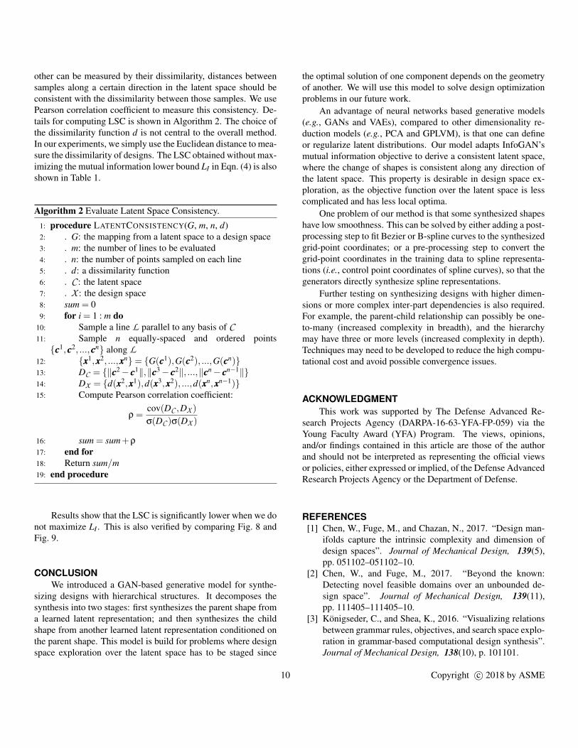
other can be measured by their dissimilarity, distances betweensamples along a certain direction in the latent space should beconsistent with the dissimilarity between those samples. We usePearson correlation coefficient to measure this consistency. De-tails for computing LSC is shown in Algorithm 2. The choice ofthe dissimilarity function d is not central to the overall method.In our experiments, we simply use the Euclidean distance to mea-sure the dissimilarity of designs. The LSC obtained without max-imizing the mutual information lower bound LI in Eqn. (4) is alsoshown in Table 1.

Algorithm 2 Evaluate Latent Space Consistency.

1: procedure LATENTCONSISTENCY(G, m, n, d)2: . G: the mapping from a latent space to a design space3: . m: the number of lines to be evaluated4: . n: the number of points sampled on each line5: . d: a dissimilarity function6: . C : the latent space7: . X : the design space8: sum = 09: for i = 1 : m do

10: Sample a line L parallel to any basis of C11: Sample n equally-spaced and ordered points{ccc1,ccc2, ...,cccn} along L

12: {xxx1,xxx2, ...,xxxn}= {G(ccc1),G(ccc2), ...,G(cccn)}13: DC = {‖ccc2− ccc1‖,‖ccc3− ccc2‖, ...,‖cccn− cccn−1‖}14: DX = {d(xxx2,xxx1),d(xxx3,xxx2), ...,d(xxxn,xxxn−1)}15: Compute Pearson correlation coefficient:

ρ =cov(DC ,DX )

σ(DC )σ(DX )

16: sum = sum+ρ

17: end for18: Return sum/m19: end procedure

Results show that the LSC is significantly lower when we donot maximize LI . This is also verified by comparing Fig. 8 andFig. 9.

CONCLUSIONWe introduced a GAN-based generative model for synthe-

sizing designs with hierarchical structures. It decomposes thesynthesis into two stages: first synthesizes the parent shape froma learned latent representation; and then synthesizes the childshape from another learned latent representation conditioned onthe parent shape. This model is build for problems where designspace exploration over the latent space has to be staged since

the optimal solution of one component depends on the geometryof another. We will use this model to solve design optimizationproblems in our future work.

An advantage of neural networks based generative models(e.g., GANs and VAEs), compared to other dimensionality re-duction models (e.g., PCA and GPLVM), is that one can defineor regularize latent distributions. Our model adapts InfoGAN’smutual information objective to derive a consistent latent space,where the change of shapes is consistent along any direction ofthe latent space. This property is desirable in design space ex-ploration, as the objective function over the latent space is lesscomplicated and has less local optima.

One problem of our method is that some synthesized shapeshave low smoothness. This can be solved by either adding a post-processing step to fit Bezier or B-spline curves to the synthesizedgrid-point coordinates; or a pre-processing step to convert thegrid-point coordinates in the training data to spline representa-tions (i.e., control point coordinates of spline curves), so that thegenerators directly synthesize spline representations.

Further testing on synthesizing designs with higher dimen-sions or more complex inter-part dependencies is also required.For example, the parent-child relationship can possibly be one-to-many (increased complexity in breadth), and the hierarchymay have three or more levels (increased complexity in depth).Techniques may need to be developed to reduce the high compu-tational cost and avoid possible convergence issues.

ACKNOWLEDGMENTThis work was supported by The Defense Advanced Re-

search Projects Agency (DARPA-16-63-YFA-FP-059) via theYoung Faculty Award (YFA) Program. The views, opinions,and/or findings contained in this article are those of the authorand should not be interpreted as representing the official viewsor policies, either expressed or implied, of the Defense AdvancedResearch Projects Agency or the Department of Defense.

REFERENCES[1] Chen, W., Fuge, M., and Chazan, N., 2017. “Design man-

ifolds capture the intrinsic complexity and dimension ofdesign spaces”. Journal of Mechanical Design, 139(5),pp. 051102–051102–10.

[2] Chen, W., and Fuge, M., 2017. “Beyond the known:Detecting novel feasible domains over an unbounded de-sign space”. Journal of Mechanical Design, 139(11),pp. 111405–111405–10.

[3] Konigseder, C., and Shea, K., 2016. “Visualizing relationsbetween grammar rules, objectives, and search space explo-ration in grammar-based computational design synthesis”.Journal of Mechanical Design, 138(10), p. 101101.


[4] Konigseder, C., Stankovic, T., and Shea, K., 2016. “Im-proving design grammar development and applicationthrough network-based analysis of transition graphs”. De-sign Science, 2.

[5] Chen, W., and Fuge, M., 2017. “Active expansion sam-pling for learning feasible domains in an unbounded in-put space”. Structural and Multidisciplinary Optimization,pp. 1–21.

[6] Kalogerakis, E., Chaudhuri, S., Koller, D., and Koltun, V.,2012. “A probabilistic model for component-based shapesynthesis”. ACM Transactions on Graphics (TOG), 31(4),p. 55.

[7] Goodfellow, I., Pouget-Abadie, J., Mirza, M., Xu, B.,Warde-Farley, D., Ozair, S., Courville, A., and Bengio, Y.,2014. “Generative adversarial nets”. In Advances in neuralinformation processing systems, pp. 2672–2680.

[8] Samareh, J. A., 2001. “Survey of shape parameterizationtechniques for high-fidelity multidisciplinary shape opti-mization”. AIAA journal, 39(5), pp. 877–884.

[9] Bellman, R., 1957. Dynamic programming. Princeton Uni-versity Press, Princeton, NY.

[10] Diez, M., Campana, E. F., and Stern, F., 2015. “Design-space dimensionality reduction in shape optimization bykarhunen–loeve expansion”. Computer Methods in AppliedMechanics and Engineering, 283, pp. 1525–1544.

[11] Chen, X., Diez, M., Kandasamy, M., Zhang, Z., Campana,E. F., and Stern, F., 2015. “High-fidelity global optimiza-tion of shape design by dimensionality reduction, meta-models and deterministic particle swarm”. EngineeringOptimization, 47(4), pp. 473–494.

[12] DAgostino, D., Serani, A., Campana, E. F., and Diez, M.,2017. “Nonlinear methods for design-space dimensionalityreduction in shape optimization”. In International Work-shop on Machine Learning, Optimization, and Big Data,Springer, pp. 121–132.

[13] Tezzele, M., Salmoiraghi, F., Mola, A., and Rozza, G.,2017. “Dimension reduction in heterogeneous parametricspaces with application to naval engineering shape designproblems”. arXiv preprint arXiv:1709.03298.

[14] Raghavan, B., Breitkopf, P., Tourbier, Y., and Villon, P.,2013. “Towards a space reduction approach for efficientstructural shape optimization”. Structural and Multidisci-plinary Optimization, 48(5), pp. 987–1000.

[15] Raghavan, B., Xia, L., Breitkopf, P., Rassineux, A., andVillon, P., 2013. “Towards simultaneous reduction of bothinput and output spaces for interactive simulation-basedstructural design”. Computer Methods in Applied Mechan-ics and Engineering, 265, pp. 174–185.

[16] Raghavan, B., Le Quilliec, G., Breitkopf, P., Rassineux,A., Roelandt, J.-M., and Villon, P., 2014. “Numerical as-sessment of springback for the deep drawing process bylevel set interpolation using shape manifolds”. Interna-

tional Journal of Material Forming, 7(4), pp. 487–501.[17] Le Quilliec, G., Raghavan, B., and Breitkopf, P., 2015. “A

manifold learning-based reduced order model for spring-back shape characterization and optimization in sheet metalforming”. Computer Methods in Applied Mechanics andEngineering, 285, pp. 621–638.

[18] Viswanath, A., J. Forrester, A., and Keane, A., 2011. “Di-mension reduction for aerodynamic design optimization”.AIAA journal, 49(6), pp. 1256–1266.

[19] Qiu, H., Xu, Y., Gao, L., Li, X., and Chi, L., 2016. “Multi-stage design space reduction and metamodeling optimiza-tion method based on self-organizing maps and fuzzy clus-tering”. Expert Systems with Applications, 46, pp. 180–195.

[20] Burnap, A., Liu, Y., Pan, Y., Lee, H., Gonzalez, R., andPapalambros, P. Y., 2016. “Estimating and exploring theproduct form design space using deep generative models”.In ASME 2016 International Design Engineering Techni-cal Conferences and Computers and Information in Engi-neering Conference, American Society of Mechanical En-gineers, pp. V02AT03A013–V02AT03A013.

[21] D’Agostino, D., Serani, A., Campana, E. F., and Diez,M., 2018. “Deep autoencoder for off-line design-space di-mensionality reduction in shape optimization”. In 2018AIAA/ASCE/AHS/ASC Structures, Structural Dynamics,and Materials Conference, p. 1648.

[22] Gmeiner, T., and Shea, K., 2013. “A spatial grammarfor the computational design synthesis of vise jaws”. InASME 2013 International Design Engineering TechnicalConferences and Computers and Information in Engineer-ing Conference, American Society of Mechanical Engi-neers, pp. V03AT03A006–V03AT03A006.

[23] Talton, J. O., Gibson, D., Yang, L., Hanrahan, P., andKoltun, V., 2009. “Exploratory modeling with collabora-tive design spaces”. ACM Transactions on Graphics-TOG,28(5), p. 167.

[24] Huang, H., Kalogerakis, E., and Marlin, B., 2015. “Analy-sis and synthesis of 3d shape families via deep-learned gen-erative models of surfaces”. In Computer Graphics Forum,Vol. 34, Wiley Online Library, pp. 25–38.

[25] Nash, C., and Williams, C. K., 2017. “The shape variationalautoencoder: A deep generative model of part-segmented3d objects”. In Computer Graphics Forum, Vol. 36, WileyOnline Library, pp. 1–12.

[26] Wu, J., Zhang, C., Xue, T., Freeman, B., and Tenenbaum,J., 2016. “Learning a probabilistic latent space of objectshapes via 3d generative-adversarial modeling”. In Ad-vances in Neural Information Processing Systems, pp. 82–90.

[27] Li, J., Xu, K., Chaudhuri, S., Yumer, E., Zhang, H., andGuibas, L., 2017. “Grass: Generative recursive autoen-coders for shape structures”. ACM Transactions on Graph-


ics (TOG), 36(4), p. 52.[28] Sinha, A., Unmesh, A., Huang, Q., and Ramani, K., 2017.

“Surfnet: Generating 3d shape surfaces using deep resid-ual networks”. In Proceedings of the IEEE Conference onComputer Vision and Pattern Recognition, pp. 6040–6049.

[29] Chaudhuri, S., Kalogerakis, E., Guibas, L., and Koltun, V.,2011. “Probabilistic reasoning for assembly-based 3d mod-eling”. In ACM Transactions on Graphics (TOG), Vol. 30,ACM, p. 35.

[30] Talton, J., Yang, L., Kumar, R., Lim, M., Goodman, N., andMech, R., 2012. “Learning design patterns with bayesiangrammar induction”. In Proceedings of the 25th annualACM symposium on User interface software and technol-ogy, ACM, pp. 63–74.

[31] Xu, K., Zhang, H., Cohen-Or, D., and Chen, B., 2012. “Fitand diverse: set evolution for inspiring 3d shape galleries”.ACM Transactions on Graphics (TOG), 31(4), p. 57.

[32] Zheng, Y., Cohen-Or, D., and Mitra, N. J., 2013. “Smartvariations: Functional substructures for part compatibil-ity”. Computer Graphics Forum (Eurographics), 32(2pt2),pp. 195–204.

[33] Fish, N., Averkiou, M., Van Kaick, O., Sorkine-Hornung,O., Cohen-Or, D., and Mitra, N. J., 2014. “Meta-representation of shape families”. ACM Transactions onGraphics (TOG), 33(4), p. 34.

[34] Kingma, D. P., and Welling, M., 2013. “Auto-encodingvariational bayes”. arXiv preprint arXiv:1312.6114.

[35] Radford, A., Metz, L., and Chintala, S., 2015. “Un-supervised representation learning with deep convolu-tional generative adversarial networks”. arXiv preprintarXiv:1511.06434.

[36] Chen, X., Duan, Y., Houthooft, R., Schulman, J., Sutskever,I., and Abbeel, P., 2016. “Infogan: Interpretable representa-tion learning by information maximizing generative adver-sarial nets”. In Advances in Neural Information ProcessingSystems, pp. 2172–2180.

[37] Wang, X., and Gupta, A., 2016. “Generative image model-ing using style and structure adversarial networks”. In Eu-ropean Conference on Computer Vision, Springer, pp. 318–335.

[38] Gielis, J., 2003. “A generic geometric transformation thatunifies a wide range of natural and abstract shapes”. Amer-ican journal of botany, 90(3), pp. 333–338.

[39] Zeiler, M. D., Krishnan, D., Taylor, G. W., and Fergus, R.,2010. “Deconvolutional networks”. In Computer Visionand Pattern Recognition (CVPR), 2010 IEEE Conferenceon, IEEE, pp. 2528–2535.

[40] Kingma, D. P., and Ba, J., 2014. “Adam: A method forstochastic optimization”. arXiv preprint arXiv:1412.6980.

[41] Sønderby, C. K., Caballero, J., Theis, L., Shi, W., andHuszar, F., 2016. “Amortised map inference for imagesuper-resolution”. arXiv preprint arXiv:1610.04490.

[42] Chollet, F., et al., 2015. Keras. https://github.com/keras-team/keras.

[43] Abadi, M., Agarwal, A., Barham, P., Brevdo, E., Chen, Z.,Citro, C., Corrado, G. S., Davis, A., Dean, J., Devin, M.,Ghemawat, S., Goodfellow, I., Harp, A., Irving, G., Isard,M., Jia, Y., Jozefowicz, R., Kaiser, L., Kudlur, M., Leven-berg, J., Mane, D., Monga, R., Moore, S., Murray, D., Olah,C., Schuster, M., Shlens, J., Steiner, B., Sutskever, I., Tal-war, K., Tucker, P., Vanhoucke, V., Vasudevan, V., Viegas,F., Vinyals, O., Warden, P., Wattenberg, M., Wicke, M.,Yu, Y., and Zheng, X., 2015. TensorFlow: Large-scale ma-chine learning on heterogeneous systems. Software avail-able from tensorflow.org.

[44] Breuleux, O., Bengio, Y., and Vincent, P., 2011. “Quicklygenerating representative samples from an rbm-derivedprocess”. Neural computation, 23(8), pp. 2058–2073.

[45] Wang, Z., Bovik, A. C., Sheikh, H. R., and Simoncelli,E. P., 2004. “Image quality assessment: from error visi-bility to structural similarity”. IEEE transactions on imageprocessing, 13(4), pp. 600–612.

[46] Higgins, I., Matthey, L., Pal, A., Burgess, C., Glorot, X.,Botvinick, M., Mohamed, S., and Lerchner, A., 2016.“beta-vae: Learning basic visual concepts with a con-strained variational framework”.

[47] Kim, H., and Mnih, A., 2018. “Disentangling by factoris-ing”. arXiv preprint arXiv:1802.05983.

[48] Chen, T. Q., Li, X., Grosse, R., and Duvenaud, D., 2018.“Isolating sources of disentanglement in variational autoen-coders”. arXiv preprint arXiv:1802.04942.


https://github.com/keras-team/keras

https://github.com/keras-team/keras

synthesizing designs with inter-part dependencies...

Documents