Synthesis and Stabilization of Complex Behaviors throughOnline Trajectory Optimization

Yuval Tassa, Tom Erez and Emanuel TodorovUniversity of Washington

Abstract— We present an online trajectory optimizationmethod and software platform applicable to complex humanoidrobots performing challenging tasks such as getting up froman arbitrary pose on the ground and recovering from largedisturbances using dexterous acrobatic maneuvers. The result-ing behaviors, illustrated in the attached video, are computedonly 7 x slower than real time, on a standard PC. The videoalso shows results on the acrobot problem, planar swimmingand one-legged hopping. These simpler problems can alreadybe solved in real time, without pre-computing anything.

I. INTRODUCTION

Online trajectory optimization, also known as Model-Predictive Control (MPC), is among the most powerfulmethods for automatic control. It retains the key benefit ofthe optimal control framework: the ability to specify high-level task goals through simple cost functions, and synthesizeall details of the behavior and control law automatically. Atthe same time MPC side-steps the main drawback of dynamicprogramming – the curse of dimensionality. This drawbackis particularly problematic for humanoid robots, whose statespace is so large that no control scheme (optimal or not) canexplore all of it in advance and prepare suitable responsesfor every conceivable situation.

MPC avoids the need for extensive exploration by post-poning the design of the policy until the last minute, andthereby finding controls only for the states that are actu-ally visited. This is done by re-optimizing the movementtrajectory and associated control sequence at each time stepof the control loop, always starting at the current stateestimate. The first control signal is applied to the system, thenext state is measured/estimated, and the procedure is thenrepeated. The trajectory optimizer is warm-started with thesolution from the previous time step, which greatly speedsup the method and often yields convergence after a single(re)optimization step. The trajectory being optimized extendsto some pre-defined horizon; thus this approach is alsoknown as receding-horizon control. A short horizon reducesthe amount of computation but results in myopic behaviors.

In domains such as chemical process control where thedynamics are sufficiently slow and smooth – and thus onlinetrajectory optimization is already feasible – MPC is themethod of choice [1]. In robotics, however, the typicaltimescales of the dynamics are orders of magnitude faster.Furthermore, many robotic tasks involve contact phenomenathat present a serious challenge to optimization-based ap-proaches. As a result, MPC is rarely used to control dexterousrobots. This is not because robotics researchers are unaware

of it or unwilling to use it, but simply because they lack thetools to make it work. While recent examples demonstratethe power of MPC applied to robotics [2], [3], much workremains to be done before it becomes a standard off-the-shelftool. When it does, we believe it will revolutionize the fieldand enable control of complex behaviors currently only seenin movies.

A. Specific contributions

The results presented here are enabled by advances onmultiple fronts. Our new physics simulator, called Mu-JoCo, was used to speed up the computation of dynamicsderivatives. MuJoCo is a C-based, platform-independent,multi-threaded simulator tailored to control applications. Wedetail several improvements to the iterative LQG method fortrajectory optimization [4] that increase its efficiency androbustness. We present a simplified model of contact dy-namics which yields a favorable trade-off between physicalrealism and speed of simulation/optimization. We introducecost functions that result in better-behaved energy landscapesand are more amenable to trajectory optimization. Finally,we describe a MATLAB-based environment where the usercan modify the dynamics model, cost function or algorithmparameters, while interacting in real time with the controlledsystem. We have found that hands-on familiarity with thevarious strengths and weaknesses of the MPC machinery isinvaluable for proper control design.

These advances have enabled us to synthesize complexhumanoid behaviors, like getting up from the ground from anarbitrary initial pose and recovering from large disturbances,in near real-time. As we show in the attached video, we caneasily solve commonly-studied problems like the “acrobot”,and also more challenging ones like swimming and one-legged hopping. These simpler problems can already besolved in real time, without pre-computing anything andwithout specifying heuristic approximations to the valuefunction. We show both robustness to state perturbations,a generic feature of the online approach, since it alwaysoptimizes the trajectory starting at the present (possiblyperturbed) state, and robustness to modeling errors – by op-timizing trajectories with respect to one model and applyingthe resulting controls to a different model

II. ONLINE TRAJECTORY OPTIMIZATION

MPC is based on repeatedly solving a finite-horizon op-timal control problem. This is done here using a trajectoryoptimization method (iterative LQG) which is the control

2012 IEEE/RSJ International Conference onIntelligent Robots and SystemsOctober 7-12, 2012. Vilamoura, Algarve, Portugal

978-1-4673-1736-8/12/S31.00 ©2012 IEEE 4906

analog of the Gauss-Newton method for nonlinear least-squares optimization. Below we provide some backgroundon finite-horizon optimal control and trajectory optimization,and then focus on the specific improvements we have madehere.

A. Finite-Horizon Optimal Control

The discrete-time dynamics

xi+1 = f(xi,ui) (1)

describe the evolution of the state x given the control u.The total cost J0 is the sum of running costs ` and final cost`f , incurred when starting from state x0 and applying thecontrol sequence U ≡ {u0,u1 . . . ,uN−1} until the horizonis reached:

J0(x,U) =

N−1∑i=0

`(xi,ui) + `f (xN ),

where the xi for i > 0 are given by (1). The solution of theoptimal control problem is the minimizing control sequence

U∗(x) ≡ argminU

J0(x,U).

By trajectory optimization, we mean finding U∗(x) for aparticular x, rather than for all possible initial states1.

B. Trajectory Optimizer

In the experiments described below we used the iterativeLinear Quadratic Gaussian (iLQG) trajectory optimizer [4].iLQG is a variant of the classic Differential Dynamic Pro-gramming (DDP) algorithm [5], the main difference beingthat only first rather than second derivatives of the dynamicsare used. This means that iLQG no longer exhibits thequadratic convergence properties of DDP, however in theMPC context the minimum is a moving target and con-vergence never actually happens, so the benefits of havingfaster dynamics evaluation greatly outweigh the decreasein performance. In our version of iLQG, we implementedseveral improvements to the regularization and line-searchaspects of the algorithm.

Let Ui ≡ {ui,ui+1 . . . ,uN−1} and define the cost-to-goJi as the partial sum of costs from i to N :

Ji(x,Ui) =

N−1∑j=i

`(xj ,uj) + `f (xN ).

The Value at time i is the cost-to-go given the minimizingcontrol sequence

V (x, i) ≡ minUi

Ji(x,Ui).

Setting V (x, N) ≡ `f (xN ), the Dynamic ProgrammingPrinciple reduces the minimization over an entire sequenceof controls to a sequence of minimizations over a singlecontrol, proceeding backwards in time:

V (x, i) = minu

[`(x,u) + V (f(x,u), i+1)] (2)

1Other trajectory optimization schemes interpret Eq. (1) as a constraintand optimize over both states and controls.

Define the argument of the minimum in (2) as a functionof perturbations around the i-th (x,u) pair:

Q(δx, δu) = `(x + δx,u + δu, i)− `(x,u, i)+ V (f(x + δx,u + δu), i+1)− V (f(x,u), i+1) (3)

and expand to second order

≈ 1

2

1δxδu

T 0 QTx QT

u

Qx Qxx Qxu

Qu Qux Quu

1δxδu

. (4)

The expansion coefficients are2

Qx = `x +fTx V′x (5a)

Qu = `u +fTuV′x (5b)

Qxx = `xx+fTx V′xxfx + V ′x · fxx (5c)

Quu = `uu+fTuV′xxfu + V ′x · fuu (5d)

Qux = `ux+fTuV′xxfx + V ′x · fux. (5e)

The last terms in (5c, 5d, 5e), which denote contraction witha tensor, are ignored in iLQG (but not in DDP). Since thestep computed by DDP is nearly identical to the full Newtonstep (see e.g. [6]), iterative LQG can be seen to correspondto the Gauss-Newton Hessian approximation.

Minimizing (4) WRT δu we have

δu∗ = argminδu

Q(δx, δu) = −Q−1uu(Qu +Quxδx), (6)

giving us an open-loop term k = −Q−1uuQu and a feedback

gain term K = −Q−1uuQux. Plugging the policy into (4), we

now have a quadratic model of the Value at time i:

∆V (i) = − 12QuQ

−1uuQu (7a)

Vx(i) = Qx −QuQ−1uuQux (7b)

Vxx(i) = Qxx−QxuQ−1uuQux. (7c)

Recursively computing the local quadratic models of V (i)and the control modifications {k(i),K(i)}, constitutes thebackward pass. Once it is completed, a forward pass com-putes a new trajectory:

x(1) = x(1) (8a)u(i) = u(i) + k(i) + K(i)(x(i)− x(i)) (8b)

x(i+1) = f(x(i), u(i)) (8c)

C. Improved Regularization

It has been shown [6] that the steps taken by DDP arecomparable to or better than a full Newton step for theentire control sequence. And as in Newton’s method, caremust be taken when the Hessian is not positive-definite orwhen the minimum is not close and the quadratic modelinaccurate. The standard regularization, proposed in [5] andfurther explored in [7], is to add a diagonal term to the localcontrol-cost Hessian

Quu = Quu + µIm, (9)

2Dropping the index i, primes denoting the next time-step: V ′ ≡ V (i+1).

4907

where µ plays the role of a Levenberg-Marquardt param-eter. This modification amounts to adding a quadratic costaround the current control-sequence, making the steps moreconservative. The drawback to this regularization scheme isthat the same control perturbation can have different effectsat different times, depending on the control-transition matrixfu. We therefore introduce a scheme that penalizes deviationsfrom the states rather than controls:

Quu = `uu + fTu (V ′xx + µIn)fu + V ′x · fuu (10a)

Qux = `ux + fTu (V ′xx + µIn)fx + V ′x · fux (10b)

k = −Q−1uuQu (10c)

K = −Q−1uuQux (10d)

This regularization amounts to placing a quadratic state-costaround the previous sequence. Unlike the standard control-based regularization, the feedback gains K do not vanish asµ→∞, but rather force the new trajectory closer to the oldone, significantly improving robustness.

Finally, we make use of the improved Value updateproposed in [4]. Examining (4, 6, 7), we see that severalcancelations of Quu and its inverse have taken place, butsince we are modifying this matrix in (9) or (10a), makingthose cancelations induces an error. The improved Valueupdate is therefore

∆V (i) = + 12k

TQuuk+kTQu (11a)

Vx(i) = Qx +KTQuuk +KTQu +QTuxk (11b)

Vxx(i) = Qxx+KTQuuK+KTQux+QTuxK. (11c)

D. Improved Line Search

The forward pass of iLQG/DDP, given by Eqs. (8) isthe key to the algorithm’s fast convergence. This is becausethe feedback gains in (8b) generate a new control sequencethat takes into account the new states as they are beingintegrated. For example when applying the algorithm to alinear-quadratic system, even a time-varying one, an exactsolution is obtained after a single iteration. The caveat isthat for a general non-linear system, when the new trajectorystrays too far from the model’s region of validity, the costmay not decrease, and divergence may occur. The solution isto introduce a backtracking line-search parameter 0 < α ≤ 1and integrate using

u(i) = u(i) + αk(i) + K(i)(x(i)− x(i)) (12)

For α = 0 the trajectory would be unchanged, but forintermediate values the resulting control step is not a simplescaled version of the full step, due to the presence offeedback. As advocated in [5], we use the expected total-cost reduction in the line-search procedure, but using theimproved formula (11a), we can derive a better estimate:

∆J(α) = α

N−1∑i=1

k(i)TQu(i) +α2

2

N−1∑i=1

k(i)TQuu(i)k(i).

When comparing the actual and expected reductions

z = [J(u1..N−1)− J(u1..N−1)]/∆J(α),

we accept the iteration only if

0 < c1 < z. (13)

E. Trajectory Optimizer Summary

A single iteration of iLQG is composed of 3 steps:

1. Derivatives: Given a nominal (x,u, i) sequence, com-pute the derivatives of ` and f in the RHS of Eq. (5). Thisstep is parallelized for all i across all available CPU cores.

2. Backward pass: Iterate Eqs. (5, 10, 11) for decreasingi = N−1, . . . 1. If a non-PD Quu is encountered, increaseµ and restart the backward pass. If successful, decrease µ.

3. Forward pass: Set α = 1. Iterate (12) and (8c) tocompute a new nominal sequence. If the integration divergedor condition (13) was not met, decrease α and restart theforward pass.

F. Regularization Schedule

The fast and accurate modification of the regularizationparameter µ in step 2 turns out to be quite importantdue to three conflicting requirements. If we are near theminimum we would like µ to quickly go to zero to enjoyfast convergence. If the back-pass fails (a non-PD Quu), wewould like it to increase very rapidly, since the minimumvalue of µ which prevents divergence is often very large.Finally, if we are in a regime where some µ > 0 is required,we would like to accurately tweak it to be as close as possibleto the minimum value, but not smaller. Our solution is to usea quadratic modification schedule. Defining some minimalvalue µmin (we use µmin = 10−6) and a minimal modificationfactor ∆0 (we use ∆0 = 2), we adjust µ as follows:

increase µ:∆← max(∆0,∆ ·∆0)

µ← max(µmin, µ ·∆)

decrease µ:

∆← min( 1∆0, ∆

∆0)

µ←

{µ ·∆ if µ ·∆ > µmin,

0 if µ ·∆ < µmin.

G. Policy-Lag and Asynchronous Control

The experiments described below are performed in sim-ulation using two instantiations of the dynamics. One isused by the controller for MPC while a different one isused to simulate the robot. A clear advantage of this isthat we can easily introduce “modeling errors” to quantifyrobustness. However, the most important quantity this allowsus to examine is the policy-lag, i.e. the time required by thecontroller to complete one MPC iteration, and its effect onperformance. During this time the previous policy is used,and at some point it stops being a good one. Note that this isa very problem-dependent quantity, since it is closely relatedto the time-variation of the policy – a smooth policy would beless sensitive to lag than a rapidly changing one. We quantifythe effects of policy lag by running the controller and

4908

simulation asynchronously on different execution threads; ifperformance is unacceptable, we artificially slow down theplant simulation. As it slows, new policies effectively arriveearlier and performance improves. Once the performance ofthe controller is acceptable, the slowdown coefficient answersthe question “How much faster should our computer be sothat this controller would work on a real robot?”

A side benefit of this architecture is that because the sep-arate execution threads communicate over TCP/IP sockets,it is trivial to run them on two different machines. In thisscenario a small, cheap CPU running on the robot performsestimation, while an MPC “policy server” runs on a morepowerful machine.

III. DYNAMICS MODELING AND SIMULATION

Online trajectory optimization is only possible when thedynamics and its derivatives can be evaluated very quickly.While some work has been done on analytical differentiation[8], it is limited to smooth dynamics and does not apply togeneral physics engines that must deal with collision de-tection, computation of contact interaction forces, enforcingnonlinear equality constraints etc. Therefore the derivativeshave to be approximated using finite-differencing. Indeedthis is where almost all the CPU time is spent. How manydynamics evaluations does MPC require? Suppose we have asystem with 20 dofs (and so the state space is 40 dimensionalbecause it includes positions and velocities) and the horizonis 50 time steps of 10ms each. Thus approximating the firstderivative at each point along the trajectory (the quantityfx above) using centered finite differencing requires 4,000dynamics evaluations per time step of the control loop. Asequential real-time simulation of these time-steps wouldtake 4 seconds, but a typical maximal policy-lag (e.g. forour humanoid problem) was on the order of 10ms, so thephysics engine must run at least 4,000 faster than real-time!Existing engines are not designed for such speed, and so wehad to implement a new full-featured physics engine fromscratch (see below). Apart from careful implementation andchoice of contact simulation methods, we use parallel pro-cessing, which is well-suited for finite differencing becausethe dynamics at many states can be evaluated in parallel,without need for synchronization or exchange of data.

A. The MuJoCo physics engine

The simulations described in this paper were carried outusing MuJoCo [9], which stands for Multi Joint dynamicswith Contact. This engine will soon be made publiclyavailable and will be free for academic research. MuJoCo isa platform-independent physics simulator tailored to controlapplications. Multi-joint dynamics are represented in jointcoordinates and computed via recursive algorithms. Thecomputation is O(n3) because the inverse inertia matrixis needed (to compute contact responses), however due totree-induced sparsity, performance is comparable to O(n)algorithms in typical usage scenarios (e.g. simulating ahumanoid). Geometry is modeled using a small library ofsmooth shapes allowing fast and accurate collision detection.

Contact responses are computed by efficient new algorithms[10]–[12] that appear to be faster and more accurate thanLCP-based methods, and are suitable for numerical opti-mization. Models are specified using either a high-level C++API or an XML file. A built-in compiler transforms theuser model into an optimized data structure used for runtimecomputation. This data structure contains a scratchpad whereall routines write their output. In this way all intermediateresults are accessible to the user, making it easy to addfunctionality. The user can modify all real-valued modelparameters in runtime without recompiling. To facilitateoptimal control applications, MuJoCo provides routines forparallel computation of the cost of a given trajectory as wellas the gradient and a Gauss-Newton approximation to theHessian. The engine can be used either as a library linkedto a user program, or via a MATLAB interface. A utility forinteractive 3D rendering is also provided.

B. Contact Modeling

Frictional contact is perhaps the most difficult aspect ofdynamics modeling. In the physical world contact phenom-ena are very stiff, i.e. they happen on very short time-scales.When bodies are modeled as infinitely stiff, the simulationbecomes discontinuous. It is possible to model compliantbodies, but this adds many degrees-of-freedom to the model.Because trajectory optimizers require derivatives of the dy-namics, discontinuous models cannot be used. Differentiablecontact models for rigid bodies fall into two categories. Thefirst type attempt to model the physics as closely as possible,e.g. with Hertz-Hunt-Crossley spring-dampers. These modelsare indeed accurate, but their stiffness demands extremelysmall time-steps, on the order of microseconds, and aretherefore prohibitively expensive. The second type of modelsare based on time stepping integrators [13], which attempt tomodel the effects of contact and friction impulses over fixed,relatively large time-steps. Because many contacts can occurin each time-step (typically on the order of 10ms), theseintegrators need to consider all contacts at once, usually bysolving a Linear Complementarity Problem. Some smoothvariants of the time stepping approach such as [10] and [12]solve an optimization problem rather than an LCP, but theresult is the same – small but cheap time-steps are exchangedfor larger but more expensive ones. Here we introduce a newcontact model, based on the time stepping formulation, thatattempts to find a balance between these two types. It is ascheap to compute as spring-damper models, yet not as stiff,producing realistic behavior for time-steps in the range of1-10ms.

C. Time-Stepping

The state x of a mechanical system is a set of generalizedpositions q and velocities v. The dynamics are given by theequations of motion

Mv = r + u

q = v,

4909

where M = M(q) is the mass matrix, r = r(q,v) the vectorof total external forces (gravity, drag, centripetal, coriolisetc.) and u is the applied control (e.g. motor torques). Fora timestep h, a semi-implicit Euler integration step (primesdenoting the next time step) is:

Mv′ = h(r + u) + Mv

q′ = q + hv′.

The unilateral constraint vector function φ(q) is a signeddistance between objects – positive for separation, zero forcontact and negative for penetration. We therefore search forimpulses λ such that

φ(q′) ≈ φ(q) + hJv′ ≥ 0,

where J = ∇φ(q). This leads to a mixed complementarityproblem for v′ and λ:

Mv′ = h(r + u) + Mv + JTλ (14a)λ ≥ 0, (14b)

φ(q) + hJv′ ≥ 0, (14c)

λT(φ(q) + hJv′) = 0. (14d)

Conditions (14b) and (14c) are read element-wise, and re-spectively constrain the contact impulse to be non-adhesive,and the distance to be non-penetrating. Condition (14d)asserts that φ(q′) > 0 (broken contact) and λ > 0 (collisionimpact), are mutually exclusive. Since the mass matrix isalways invertible, we can solve (14a) for v′, and plug into(14c). Defining

A = JM−1JT (15a)

b = φ(q)/h+ J(v + hM−1(r + u)), (15b)

we can now write (14) in standard LCP form:

Find λ s.t. 0 ≤ λ ⊥ Aλ+ b ≥ 0. (16)

D. Diagonal Approximation

Instead of solving (16) simultaneously for all the impulsesλ, we first take the diagonal approximation to A, and solveindependently for each component3:

λi = −bi/Aii.

The λi are the impulses that would make the φi vanish,regardless of sign. We now scale these by some factor 0 <η < 1 and make them positive with a smooth approximationto max(·, 0):

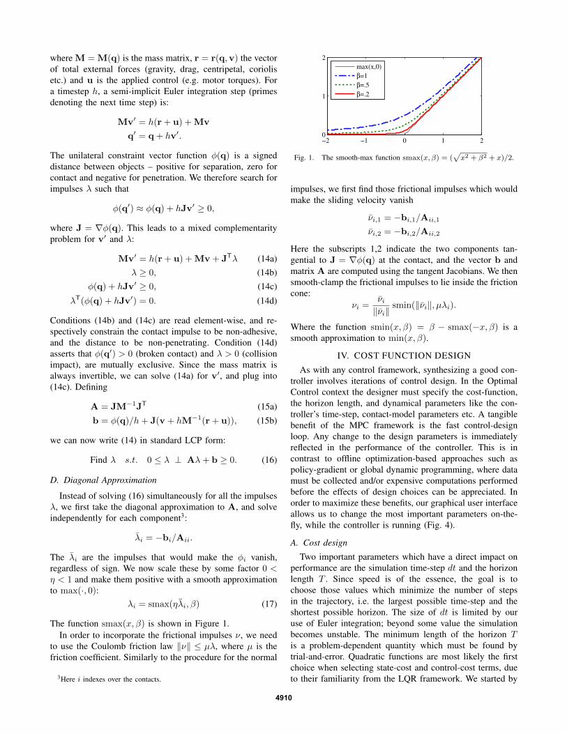
λi = smax(ηλi, β) (17)

The function smax(x, β) is shown in Figure 1.In order to incorporate the frictional impulses ν, we need

to use the Coulomb friction law ‖ν‖ ≤ µλ, where µ is thefriction coefficient. Similarly to the procedure for the normal

3Here i indexes over the contacts.

−2 −1 0 1 20

1

2

max(x,0)

β=1

β=.5

β=.2

Fig. 1. The smooth-max function smax(x, β) = (√x2 + β2 + x)/2.

impulses, we first find those frictional impulses which wouldmake the sliding velocity vanish

νi,1 = −bi,1/Aii,1

νi,2 = −bi,2/Aii,2

Here the subscripts 1,2 indicate the two components tan-gential to J = ∇φ(q) at the contact, and the vector b andmatrix A are computed using the tangent Jacobians. We thensmooth-clamp the frictional impulses to lie inside the frictioncone:

νi =νi‖νi‖

smin(‖νi‖, µλi).

Where the function smin(x, β) = β − smax(−x, β) is asmooth approximation to min(x, β).

IV. COST FUNCTION DESIGN

As with any control framework, synthesizing a good con-troller involves iterations of control design. In the OptimalControl context the designer must specify the cost-function,the horizon length, and dynamical parameters like the con-troller’s time-step, contact-model parameters etc. A tangiblebenefit of the MPC framework is the fast control-designloop. Any change to the design parameters is immediatelyreflected in the performance of the controller. This is incontrast to offline optimization-based approaches such aspolicy-gradient or global dynamic programming, where datamust be collected and/or expensive computations performedbefore the effects of design choices can be appreciated. Inorder to maximize these benefits, our graphical user interfaceallows us to change the most important parameters on-the-fly, while the controller is running (Fig. 4).

A. Cost design

Two important parameters which have a direct impact onperformance are the simulation time-step dt and the horizonlength T . Since speed is of the essence, the goal is tochoose those values which minimize the number of stepsin the trajectory, i.e. the largest possible time-step and theshortest possible horizon. The size of dt is limited by ouruse of Euler integration; beyond some value the simulationbecomes unstable. The minimum length of the horizon Tis a problem-dependent quantity which must be found bytrial-and-error. Quadratic functions are most likely the firstchoice when selecting state-cost and control-cost terms, dueto their familiarity from the LQR framework. We started by

4910

using these, but have subsequently come to prefer differentfunctions.

For the state-cost, we use the “smooth-abs” function

`(x) =√x2 + α2 − α.

This function, shown in Figure 2, is smooth in an α-sized neighborhood of the origin, and then becomes linearfurther away. The linear regime offers two advantages. Thefirst is that in the finite-horizon formulation, a change inx integrated over the trajectory leads to a fixed changein total cost, and therefore encourages periodic behaviour.For example if x is the distance from some target, thesame behaviour would emerge at different distances. Thesecond benefit has to do with the relative weighting of state-cost terms. Because the linear regime is unit-preserving, therelative weight of different cost terms maintains the originalrelationship of the underlying units. For example if one costterm encodes reaching a target in the xy plane while anotherencodes keeping the torso at certain height z, it is easier tofind the appropriate weights for these terms because theircontribution, in the linear regime, is proportional to distance.

−3 −2 −1 0 1 2 30

1

2

|x|

α=2

α=1

α=.2

Fig. 2. The smooth-abs cost function `(x) =√x2 + α2 − α.

For the control-cost term the quadratic works well inthe sense of finding a solution, however that solution isnot always desirable. It is often the case that controls areinherently limited and ideally one would want a control costthat grows to infinity at these limits. The problem with suchfunctions is that the trajectory optimizer will often try tospecify a control that is outside the limits, leading to infiniteor undefined total cost and wasting an MPC iteration. Instead,we use the function

`(u) = α2(cosh(u/α)− 1).

This function, shown in Figure 3, has a second-derivative of1 at the origin and then grows exponentially beyond an α-sized neighborhood. By varying α, we can easily limit thecontrols to a particular volume of u-space, without riskingundefined or infinite values.

−3 −2 −1 0 1 2 30

1

2

u2/2

α=1

α=.3

α=.1

Fig. 3. The control-limiting cost function `(u) = α2(cosh(u/α)− 1).

B. Interactive GUI

We implemented a MATLAB-based GUI shown in Figure 4.It enabled us to explore the effects of dynamics and algorithmparameters interactively. The ability to modify the parametersin real time and observe their effect on the controller provedto be invaluable for proper tuning. Note that we have two setsof dynamics parameters, one used by the optimizer and theother by the simulator. By setting them to different values,we can simulate the effects of model errors.

V. RESULTS

The power of our resulting controller can only be fullyappreciated by watching the video, also available here:

www.cs.washington.edu/homes/tassa/media/IROS12.mp4

As seen in the video, we experimented with several controlproblems, but due to space constraints we will focus hereonly on the most challenging one – a 22-DoF humanoidmodel. It is 1.6m tall and weighs 55Kg. The hip, shoulderand abdomen joints are 2-DoF while elbows, knees andankles are 1-DoF, see Fig 4.

Fig. 4. Left: Our MATLAB-based GUI for real-time exploration of problemand algorithm parameters. Right: the 22-DoF humanoid model at its initialconfiguration, with visualization of the 16 joints.

The state-cost is composed of 4 terms. The first termpenalizes the horizontal distance (in the xy-plane) betweenthe center-of-mass (CoM) and the mean of the feet positions.The second term penalizes the horizontal distance betweenthe torso and the CoM. The third penalizes the verticaldistance between the torso and a point 1.3m over the mean ofthe feet. All three terms use the smooth-abs norm (Figure 2).

4911

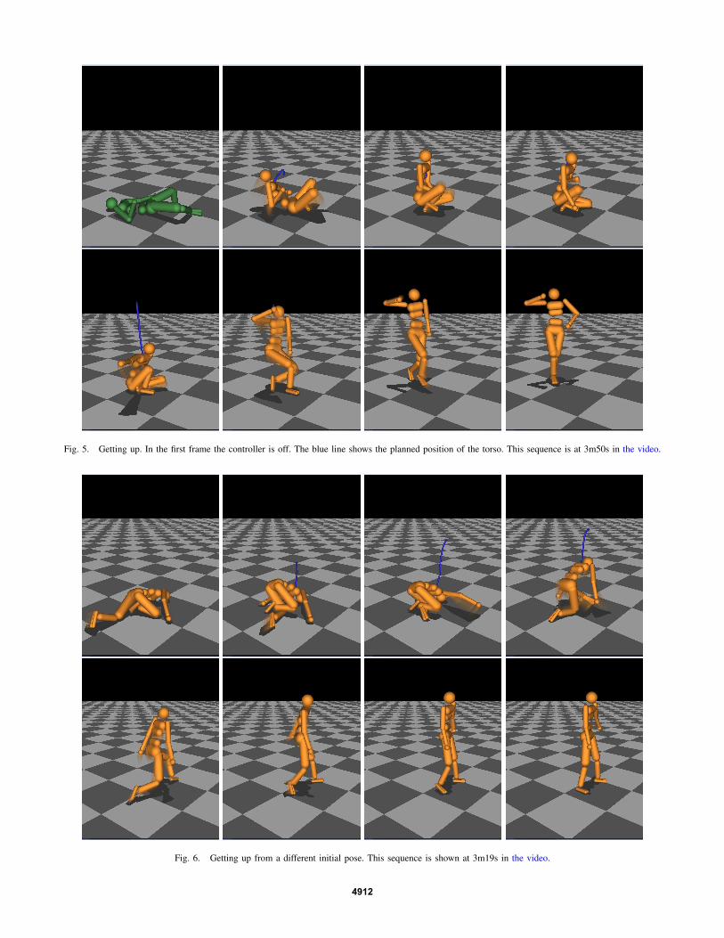
Fig. 5. Getting up. In the first frame the controller is off. The blue line shows the planned position of the torso. This sequence is at 3m50s in the video.

Fig. 6. Getting up from a different initial pose. This sequence is shown at 3m19s in the video.

4912

The fourth state-cost term is a quadratic penalty on thehorizontal CoM velocity. We tried several combinations ofstate-cost terms, all designed so that cost is small when thehumanoid is standing still. Though we finally picked the onedescribed above, it was not difficult to find a cost whichwould promote getting-up, and other variations worked well.

The dynamics of the controller and the simulator weredifferent in two important respects. First, the time step of thesimulator was 2ms while the controller’s was 8ms. Second,we used η = 0.7 for the simulator and η = 0.4 for thecontroller (see Eq. (17), we used β = 1 for both models).Both of these choices had the effect of stiffer contact inthe plant than in the model. Stiff contact and small timesteps in the plant led to realistic contact and friction, whilelarger time steps and smoother contact for the led to an easieroptimization problem for the controller.

The planning horizon was 500 milliseconds. Performancedegraded for shorter horizons, but did not qualitatively im-prove for longer ones.

The most significant fact about our parameter choices wasthat they were fairly arbitrary. Performance was qualitativelysimilar for wide range of parameters for both the costand dynamics. Additionally, the sequences shown in thevideo and in Figures 5 and 6, were not exceptional orcarefully selected. They show the typical performance of thecontroller.

The maximal policy-lag which admitted a qualitativelyreasonable policy was about 20ms. Since the actual iterationtime was 140ms, the required slowdown was x 7.

VI. FUTURE DIRECTIONS

One way to speed up MPC is to provide an approximationto the optimal value function, and use it as final cost appliedat the horizon. Specifically, this makes it possible to useshorter horizons while avoiding myopic behavior. If the exactoptimal value function is available, MPC will return theoptimal controls, but in that case we do not it, becauseone-step greedy optimization recovers the optimal controlsgiven the optimal value function. Better approximations willgenerally yield better performance. An example of suchapproximation is computer chess, where simple heuristicsfor evaluating board configurations are very effective whencombined with sufficiently-deep search. A robotics exampleis [14], where ball-bouncing is achieved via MPC, using aheuristic that specifies what is a good way to hit a ball. Suchapproximations can clearly help, however they are orthogonalto the issue of efficient trajectory optimization in the MPCcontext. Therefore in this paper we avoided using informativefinal costs; instead we simply set the final cost equal to therunning cost. Thus the results reported here are in some senseworst-case results, and the performance of our method canbe improved by using domain-specific approximations to theoptimal value function. Nevertheless we found it useful tofocus on this worst case, because it enables us to isolatethe trajectory optimization machinery and refine it, and alsobecause we prefer methods that are fully automated and donot rely on a fortuitous guess of the optimal value function.

VII. CONCLUSION

We presented an MPC method applicable to humanoidrobots performing complex tasks such as getting up fromthe ground and rejecting large perturbations. We were ableto achieve near-real-time performance on a standard desktopmachine, without using any approximations to the optimalvalue function – which can presumably speed up our methodeven further. This was possible due to multiple improvementsthroughout the MPC pipeline, including the trajectory op-timization algorithm, the physics engine, and cost functiondesign. With some additional refinements, we believe that ourMPC methodology will be applicable to complex humanoidrobots. This of course requires a sufficiently accurate dynam-ics model, which is beyond the scope of the present paper.We show however that our approach is reasonably robustto model errors and state perturbations. How well it willwork on physical robots performing different tasks remainsto be seen, and the answer may depend on the hardware andtask. Nevertheless, having the tools to apply MPC to complexrobots is likely to enable many robotic control tasks that arebeyond the reach of existing methods for real-time feedbackcontrol.

REFERENCES

[1] M. Diehl, H. Ferreau, and N. Haverbeke, “Efficient numerical methodsfor nonlinear mpc and moving horizon estimation,” Nonlinear ModelPredictive Control, p. 391, 2009.

[2] P. Abbeel, A. Coates, M. Quigley, and A. Y. Ng, “An application ofreinforcement learning to aerobatic helicopter flight,” in Advances inNeural Information Processing Systems 19: Proceedings of the 2006Conference, 2007, p. 1.

[3] T. Erez, Y. Tassa, and E. Todorov, “Infinite horizon model predictivecontrol for nonlinear periodic tasks,” Manuscript under review, 2011.

[4] E. Todorov and W. Li, “A generalized iterative LQG method forlocally-optimal feedback control of constrained nonlinear stochasticsystems,” in Proceedings of the 2005, American Control Conference,2005., Portland, OR, USA, 2005, pp. 300–306.

[5] D. H. Jacobson and D. Q. Mayne, Differential Dynamic Programming.Elsevier, 1970.

[6] L. Z. Liao and C. A. Shoemaker, “Advantages of differential dynamicprogramming over newton’s method for discrete-time optimal controlproblems,” Cornell University, Ithaca, NY, 1992.

[7] ——, “Convergence in unconstrained discrete-time differential dy-namic programming,” IEEE Transactions on Automatic Control,vol. 36, no. 6, p. 692, 1991.

[8] G. Sohl and J. Bobrow, “A recursive multibody dynamics and sensi-tivity algorithm for branched kinematic chains,” Journal of DynamicSystems, Measurement, and Control, vol. 123, p. 391, 2001.

[9] E. Todorov, T. Erez, and Y. Tassa, “MuJoCo: a physics engine formodel-based control,” in Proceedings of the 2012 IEEE/RSJ Interna-tional Conference on Intelligent Robots and Systems, 2012.

[10] Y. Tassa and E. Todorov, “Stochastic complementarity for local controlof discontinuous dynamics,” in Proceedings of Robotics: Science andSystems (RSS), 2010.

[11] E. Todorov, “Implicit nonlinear complementarity: a new approachto contact dynamics,” in International Conference on Robotics andAutomation, 2010.

[12] ——, “A convex, smooth and invertible contact model for trajectoryoptimization,” in 2011 IEEE International Conference on Robotics andAutomation (ICRA). IEEE, May 2011, pp. 1071–1076.

[13] D. E. Stewart, “Rigid-body dynamics with friction and impact,” SIAMReview, vol. 42, no. 1, pp. 3–39, Jan. 2000.

[14] P. Kulchenko and E. Todorov, “First-exit model predictive controlof fast discontinuous dynamics: Application to ball bouncing,” inRobotics and Automation (ICRA), 2011 IEEE International Conferenceon, 2011, p. 21442151.

4913