synchronization in intermittent turbulence and...

sid.inpe.br/mtc-m19@80/2010/04.29.12.38-TDI

SYNCHRONIZATION IN INTERMITTENT

TURBULENCE AND SPATIOTEMPORAL CHAOS IN

THE SOLAR TERRESTRIAL ENVIRONMENT

Rodrigo Andres Miranda Cerda

Doctorate Thesis at Post Graduation Course in Space Geophysics, advised by Drs.

Abraham Chian Long-Chian, and Erico Luiz Rempel, approved in May 01, 2010.

URL of the original document:

<http://urlib.net/8JMKD3MGP7W/37DH6JE >

INPE

Sao Jose dos Campos

2010

http://urlib.net/8JMKD3MGP7W/37DH6JE

PUBLISHED BY:

Instituto Nacional de Pesquisas Espaciais - INPE

Gabinete do Diretor (GB)

Servico de Informacao e Documentacao (SID)

Caixa Postal 515 - CEP 12.245-970

Sao Jose dos Campos - SP - Brasil

Tel.:(012) 3208-6923/6921

Fax: (012) 3208-6919

E-mail: [email protected]

BOARD OF PUBLISHING AND PRESERVATION OF INPE INTEL-

LECTUAL PRODUCTION (RE/DIR-204):

Chairperson:

Dr. Gerald Jean Francis Banon - Coordenacao Observacao da Terra (OBT)

Members:

Dra Inez Staciarini Batista - Coordenacao Ciencias Espaciais e Atmosfericas (CEA)

Dra Maria do Carmo de Andrade Nono - Conselho de Pos-Graduacao

Dra Regina Celia dos Santos Alvala - Centro de Ciencia do Sistema Terrestre (CST)

Marciana Leite Ribeiro - Servico de Informacao e Documentacao (SID)

Dr. Ralf Gielow - Centro de Previsao de Tempo e Estudos Climaticos (CPT)

Dr. Wilson Yamaguti - Coordenacao Engenharia e Tecnologia Espacial (ETE)

Dr. Horacio Hideki Yanasse - Centro de Tecnologias Especiais (CTE)

DIGITAL LIBRARY:

Dr. Gerald Jean Francis Banon - Coordenacao de Observacao da Terra (OBT)


Deicy Farabello - Centro de Previsao de Tempo e Estudos Climaticos (CPT)

DOCUMENT REVIEW:


Yolanda Ribeiro da Silva Souza - Servico de Informacao e Documentacao (SID)

ELECTRONIC EDITING:

Viveca Sant´Ana Lemos - Servico de Informacao e Documentacao (SID)

sid.inpe.br/mtc-m19@80/2010/04.29.12.38-TDI

SYNCHRONIZATION IN INTERMITTENT

TURBULENCE AND SPATIOTEMPORAL CHAOS IN

THE SOLAR TERRESTRIAL ENVIRONMENT

Rodrigo Andres Miranda Cerda

Doctorate Thesis at Post Graduation Course in Space Geophysics, advised by Drs.

Abraham Chian Long-Chian, and Erico Luiz Rempel, approved in May 01, 2010.

URL of the original document:

<http://urlib.net/8JMKD3MGP7W/37DH6JE >

INPE

Sao Jose dos Campos

2010

http://urlib.net/8JMKD3MGP7W/37DH6JE

Cataloging in Publication Data

Miranda Cerda, Rodrigo Andres.M672s Synchronization in intermittent turbulence and spatiotempo-

ral chaos in the solar terrestrial environment / Rodrigo AndresMiranda Cerda. – Sao Jose dos Campos : INPE, 2010.

153 p. ; (sid.inpe.br/mtc-m19@80/2010/04.29.12.38-TDI)

Thesis (Doctorate Thesis in Spatial Geophysics) – NationalInstitute For Space Research, Sao Jose dos Campos, 2010.

Advisers : Drs. Abraham Chian Long-Chian, and Erico LuizRempel.

1. Synchronization. 2. Turbulence. 3. Spatiotemporal chaos.4. Intermittency. 5. Coherents structures. I.Tıtulo.

CDU 523.62-726

Copyright c© 2010 do MCT/INPE. Nenhuma parte desta publicacao pode ser reproduzida, ar-mazenada em um sistema de recuperacao, ou transmitida sob qualquer forma ou por qualquermeio, eletronico, mecanico, fotografico, reprografico, de microfilmagem ou outros, sem a permissaoescrita do INPE, com excecao de qualquer material fornecido especificamente com o proposito deser entrado e executado num sistema computacional, para o uso exclusivo do leitor da obra.

Copyright c© 2010 by MCT/INPE. No part of this publication may be reproduced, stored in aretrieval system, or transmitted in any form or by any means, electronic, mechanical, photocopying,recording, microfilming, or otherwise, without written permission from INPE, with the exceptionof any material supplied specifically for the purpose of being entered and executed on a computersystem, for exclusive use of the reader of the work.

ii

To Amélia, my father Eduardo, my mother María Cecilia,my brother Eduardo and my sister Carolina,

and to all the victims of the 2010 Chilean earthquake.

ACKNOWLEDGEMENTS

First of all, I would like to thank my beloved girlfriend Amelia Naomi Onohara, for

her love and patience, for staying with me during sunny days, under the rain and

during storms.

I would like to thank my supervisors, Prof. Abraham Chian-Long Chian, and Prof.

Erico Luiz Rempel, for their patience, advice, incentive and valuable friendship.

I thank Prof. Michio Yamada, Dr. Yoshitaka Saiki and RIMS of Kyoto University

for their kind hospitality.

To Coordenacao de Aperfeicoamento de Pessoal de Nıvel Superior (CAPES) and

Conselho Nacional de Desenvolvimento Cientıfico e Tecnologico (CNPq), for finan-

cial support.

To Dr. Daiki Koga, Dr. Felix Borotto, and Mr. Pablo Munoz for their advice and

friendship.

I would like to thank Dr. Ricardo Monreal and Ms. Cecilia Llop for their incentive

to enter the PhD course.

To Dr. Ezequiel Echer, Prof. Roberto Bruno, Prof. Kristoff Stasiewicz, Dr. Olga

Alexandrova, Prof. Melvin Goldstein, Prof. Bruce T. Tsurutani and Prof. Charles

Meneveau for stimulating discussions.

To the Cluster FGM and CIS instrument teams, the ACE MAG and SWEPAM

instrument teams, the SOHO FGM instrument team, Prof. Fernando Ramos, Dr.

Mauricio Bolzan and Prof. Nalin B. Trivedi for providing the data used in this thesis.

And at last but not least, I would like to thank all my colleagues and friends at

INPE: Aline, Marlos, Valentin, Wanderson, Mauricio, Sergio, Fabio and Yang, and

my friends I met in Japan: Azusa, Inubushi, Ichiyama, Mauricio, Fabricio, Fabian

and the rest of the “latino mafia” at Kyoto University. Thanks for your friendship.

ABSTRACT

In this work we analyze synchronization due to multiscale interactions in obser-vations of intermittent turbulence and numerical simulations of spatiotemporal in-termittency in neutral fluids and space plasmas. This study is carried out in twoparts. First, we apply two distinct nonlinear techniques, kurtosis and phase coher-ence index, to measure the degree of non-Gaussianity and phase synchronizationof intermittent magnetic field turbulence observed in the ambient solar wind, inthe solar photosphere and in the ground, and intermittent atmospheric turbulenceobserved in the Amazon rain forest canopy. Next, we analyze a spatially-extendedmodel of nonlinear waves in fluids and plasmas to identify transient coherent struc-tures responsible for the on-off spatiotemporal intermittency observed in the timeseries of energy. We quantify the degree of amplitude-phase synchronization usingthe power-phase spectral entropy at the onset of spatiotemporal chaos. The observa-tional and theoretical results indicate that the amplitude-phase synchronization maybe the origin of intermittency in fully-developed turbulence in the solar-terrestrialenvironment.

SINCRONIZACAO EM TURBULENCIA INTERMITENTE E CAOSESPACO-TEMPORAL NO AMBIENTE SOLAR-TERRESTRE

RESUMO

Neste trabalho de Tese analisamos a sincronizacao devido a interacoes entre escalasem observacoes de turbulencia intermitente e em simulacoes numericas de inter-mitencia espaco-temporal em fluidos neutros e plasmas espaciais. Este estudo e feitoem duas partes. Primeiro, aplicamos duas tecnicas nao-lineares, curtose e ındice decoerencia de fase, para medir o grau de nao-Gaussianidade e sincronizacao de faseda turbulencia de campo magnetico intermitente observada no vento solar, na foto-sfera solar e no solo, e da turbulencia atmosferica intermitente observada na copada floresta Amazonica. Depois, analisamos um modelo espacialmente estendido deondas nao-lineares em fluidos e plasmas para identificar estruturas coerentes tran-sientes, responsaveis pela intermitencia on-off espaco-temporal observada nas seriestemporais da energia. Quantificamos o grau de sincronizacao de amplitude e faseusando a entropia espectral de potencia e de fase no regime logo depois da transicaopara caos espaco-temporal. Os resultados observacionais e teoricos indicam que asincronizacao de amplitude e fase pode ser a origem da intermitencia na turbulenciacompletamente desenvolvida no ambiente solar-terrestre.

CONTENTS

Pag.

LIST OF FIGURES

LIST OF TABLES

LIST OF ABBREVIATIONS

1 INTRODUCTION . . . . . . . . . . . . . . . . . . . . . . . . . . . 25

2 FUNDAMENTALS OF INTERMITTENT TURBULENCE

AND SPATIOTEMPORAL INTERMITTENCY . . . . . . . . . 29

2.1 Concepts of intermittent turbulence . . . . . . . . . . . . . . . . . . . . . 29

2.1.1 Kolmogorov’s 1941 theory . . . . . . . . . . . . . . . . . . . . . . . . . 29

2.1.2 Taylor hypothesis . . . . . . . . . . . . . . . . . . . . . . . . . . . . . . 31

2.1.3 Higher-order structure functions . . . . . . . . . . . . . . . . . . . . . . 32

2.1.4 Phase coherence index . . . . . . . . . . . . . . . . . . . . . . . . . . . 33

2.2 Concepts of spatiotemporal intermittency . . . . . . . . . . . . . . . . . 35

2.2.1 Numerical detection of chaotic saddles . . . . . . . . . . . . . . . . . . 37

2.2.2 Mathematical representation of wave variables . . . . . . . . . . . . . . 38

2.2.3 Fourier-Lyapunov decomposition . . . . . . . . . . . . . . . . . . . . . 42

2.3 Synchronization of chaotic oscillators . . . . . . . . . . . . . . . . . . . . 45

3 OBSERVATION OF SYNCHRONIZATION IN INTERMIT-

TENT TURBULENCE . . . . . . . . . . . . . . . . . . . . . . . . 51

3.1 Synchronization in magnetic field turbulence . . . . . . . . . . . . . . . . 53

3.1.1 non-ICME event . . . . . . . . . . . . . . . . . . . . . . . . . . . . . . 53

3.1.2 ICME event . . . . . . . . . . . . . . . . . . . . . . . . . . . . . . . . . 72

3.2 Synchronization in atmospheric turbulence . . . . . . . . . . . . . . . . . 79

3.3 Discussion . . . . . . . . . . . . . . . . . . . . . . . . . . . . . . . . . . . 85

4 THEORY OF SYNCHRONIZATION IN SPATIOTEMPORAL

INTERMITTENCY . . . . . . . . . . . . . . . . . . . . . . . . . . 91

4.1 Spatiotemporal intermittency and chaotic saddles in the Benjamin-Bona-

Mahony (BBM) equation . . . . . . . . . . . . . . . . . . . . . . . . . . . 91

4.2 Synchronization in the BBM equation . . . . . . . . . . . . . . . . . . . 102

5 CONCLUSION . . . . . . . . . . . . . . . . . . . . . . . . . . . . . 115

REFERENCES . . . . . . . . . . . . . . . . . . . . . . . . . . . . . . . 119

7 APPENDIX A - SYNCHRONIZATION IN THE SOLAR PHO-

TOSPHERE BEFORE AND AFTER A SOLAR FLARE EVENT135

8 APPENDIX B - KOLMOGOROV 1941 THEORY AND ITS EX-

TENSION TO MAGNETOHYDRODYNAMICS . . . . . . . . . 139

8.1 Neutral fluids . . . . . . . . . . . . . . . . . . . . . . . . . . . . . . . . . 139

8.2 Magnetized flows . . . . . . . . . . . . . . . . . . . . . . . . . . . . . . . 142

9 APPENDIX C - SHANNON ENTROPY . . . . . . . . . . . . . . 145

10 APPENDIX D - WAVE ENERGY IN THE BENJAMIN-BONA-

MAHONY EQUATION . . . . . . . . . . . . . . . . . . . . . . . . 149

11 LIST OF PUBLICATIONS . . . . . . . . . . . . . . . . . . . . . . 153

LIST OF FIGURES

Pag.

2.1 Generation of a phase-randomized surrogate and a phase-correlated sur-

rogate from the original data set . . . . . . . . . . . . . . . . . . . . . . . 34

2.2 Maximum transversal Lyapunov exponent λ⊥ as a function of the cou-

pling parameter ε . . . . . . . . . . . . . . . . . . . . . . . . . . . . . . . 47

2.3 Projections of chaotic orbits for ε = 0.1 corresponding to (a) the first

coupled Rossler oscillator, (b) the second coupled Rossler oscillator and

(c) the second coupled Rossler oscillator. (d) The same orbit projected

on the (x1, x2) plane. . . . . . . . . . . . . . . . . . . . . . . . . . . . . . 49

2.4 Projections of chaotic orbits for ε = 0.025 of (a) the first coupled Rossler

oscillator, (b) the second coupled Rossler oscillator and (c) the second

coupled Rossler oscillator. (d) The same orbit projected on the (x1, x2)

plane. . . . . . . . . . . . . . . . . . . . . . . . . . . . . . . . . . . . . . 49

3.1 Orbit trace of Cluster and spacecraft position of ACE from 19:40:40 UT

on 1 February 2002 to 03:56:38 UT on 3 February 2002 . . . . . . . . . . 56

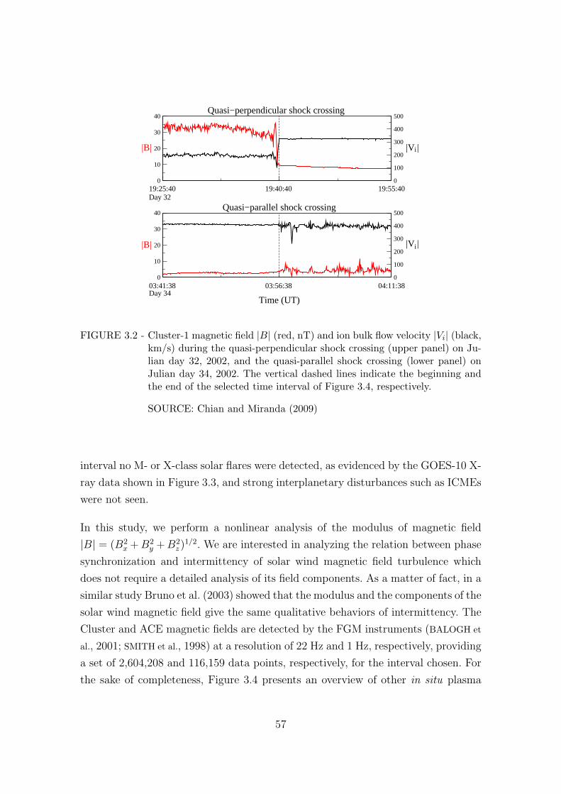
3.2 Cluster-1 magnetic field and ion bulk flow velocity during the quasi-

perpendicular shock crossing on Julian day 32, 2002, and the quasi-

parallel shock crossing on Julian day 34, 2002. . . . . . . . . . . . . . . . 57

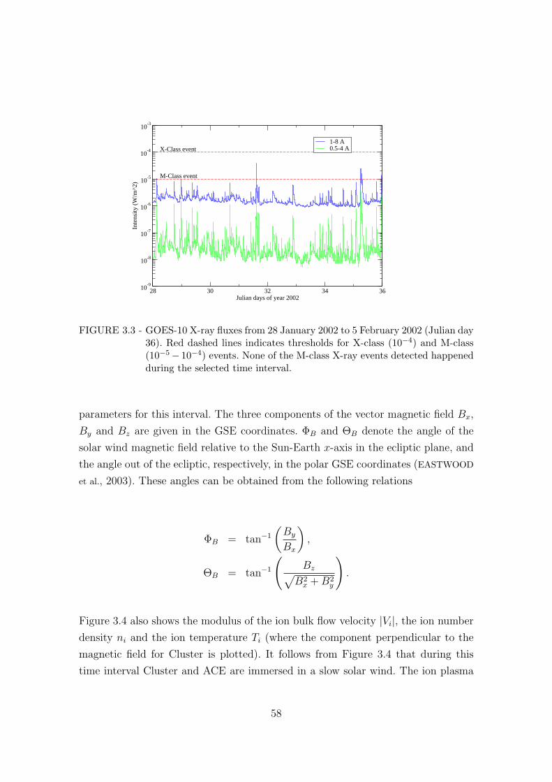
3.3 GOES-10 X-ray fluxes from 28 January 2002 to 5 February 2002 . . . . . 58

3.4 ACE and Cluster-1 magnetic field and plasma parameters for the selected

time interval. . . . . . . . . . . . . . . . . . . . . . . . . . . . . . . . . . 59

3.5 Time series of the modulus of magnetic field of Cluster-1 and ACE, after

removing the trend. . . . . . . . . . . . . . . . . . . . . . . . . . . . . . . 61

3.6 Power spectral density (PSD) of |B| for Cluster-1 and ACE, and Com-

pensated PSD for Cluster-1 and ACE. . . . . . . . . . . . . . . . . . . . 62

3.7 Power spectral density of |B| for Cluster-1 and ACE, and their confidence

intervals. . . . . . . . . . . . . . . . . . . . . . . . . . . . . . . . . . . . . 63

3.8 Scale dependence of the normalized magnetic field-differences of Cluster

and ACE. . . . . . . . . . . . . . . . . . . . . . . . . . . . . . . . . . . . 65

3.9 The integrand of Equation 3.2, for p = 0 and p = 4, determined from the

magnetic field fluctuations of Cluster-1 and ACE. . . . . . . . . . . . . . 67

3.10 Variations of structure functions with timescale τ calculated from the

magnetic field fluctuations of Cluster-1 and ACE, and structure functions

after applying the Extended Self-Similarity technique. . . . . . . . . . . . 68

3.11 Scaling exponent ζ of the p-th order structure function for Cluster-1 and

ACE magnetic field fluctuations. . . . . . . . . . . . . . . . . . . . . . . 70

3.12 Kurtosis and phase coherence index of |B| measured by Cluster-1 and

ACE. . . . . . . . . . . . . . . . . . . . . . . . . . . . . . . . . . . . . . . 71

3.13 SOHO MDI solar image, kurtosis and the phase coherence index of AR

09802 and a quiet region. . . . . . . . . . . . . . . . . . . . . . . . . . . . 73

3.14 SOHO MDI solar image, kurtosis and the phase coherence index of AR

10720 and a quiet region. . . . . . . . . . . . . . . . . . . . . . . . . . . . 73

3.15 Time series of |B| measured by ACE and Cluster on 1-3 February 2002,

and kurtosis and the phase coherence index of |B|. . . . . . . . . . . . . 76

3.16 Time series of |B| measured by ACE on 21-22 January 2005, and kurtosis

and the phase coherence index of |B|. . . . . . . . . . . . . . . . . . . . . 76

3.17 Time series, kurtosis and the phase coherence index of |B| measured by

ACE, and |B| of the Earth’s geomagnetic field measured by a ground

magnetometer at Ji-Parana on 1-3 February 2002. . . . . . . . . . . . . . 77

3.18 Time series |B| measured by ACE, and time series, kurtosis and phase

coherence index of the modulus of the Earth’s geomagnetic field measured

by a ground magnetometer at Vassouras on 1-3 February 2002. . . . . . . 77

3.19 Time series of temperature and vertical wind velocity above and within

the Amazon canopy. . . . . . . . . . . . . . . . . . . . . . . . . . . . . . 80

3.20 Scale dependence of the normalized temperature-difference and the nor-

malized vertical wind velocity-difference above the Amazon forest canopy. 81

3.21 Scale dependence of the normalized temperature-difference and the nor-

malized vertical wind velocity-difference within the Amazon forest canopy. 82

3.22 PDF of the normalized vertical wind velocity-difference and the normal-

ized temperature-difference above the Amazon forest canopy. . . . . . . . 83

3.23 PDF of the normalized vertical wind velocity-difference and the normal-

ized temperature-difference within the Amazon forest canopy. . . . . . . 84

3.24 Kurtosis and phase coherence index of vertical wind velocities and tem-

peratures above and within the Amazon forest canopy. . . . . . . . . . . 85

3.25 Kurtosis and phase coherence index of vertical wind velocities and tem-

peratures above and within the Amazon forest canopy. . . . . . . . . . . 86

4.1 Spatiotemporal patterns of the regularized long wave equation for ε =

0.199, and ε = 0.201. . . . . . . . . . . . . . . . . . . . . . . . . . . . . . 95

4.2 Time-averaged power spectra in the k wavenumber domain for ε = 0.199

and ε = 0.201. . . . . . . . . . . . . . . . . . . . . . . . . . . . . . . . . . 96

4.3 Time-averaged power spectral entropy as a function of the driver ampli-

tude ε. . . . . . . . . . . . . . . . . . . . . . . . . . . . . . . . . . . . . . 97

4.4 Time series of wave energy E and the maximum peak value of power

spectrum h. . . . . . . . . . . . . . . . . . . . . . . . . . . . . . . . . . . 99

4.5 Projections of attracting and non-attracting chaotic sets for the regular-

ized long wave equation, for ε = 0.199 and ε = 0.201. . . . . . . . . . . . 101

4.6 Average duration of laminar intervals τ as a function of the departure

from the critical value of the control parameter. . . . . . . . . . . . . . . 102

4.7 Amplitude and phase dynamics of the spatiotemporally chaotic attractor

after the crisis-like transition (ε = 0.20005). . . . . . . . . . . . . . . . . 104

4.8 Three-dimensional projections of attracting and non-attracting chaotic

sets for the regularized long wave equation, for ε = 0.199 and ε = 0.20005.105

4.9 Amplitude and phase dynamics of the temporally chaotic saddle and the

spatiotemporally chaotic saddle after the crisis-like transition. . . . . . . 106

4.10 Time-averaged power spectra and phase-difference spectra of STCA,

STCS and TCS. . . . . . . . . . . . . . . . . . . . . . . . . . . . . . . . . 108

4.11 Spectrum of positive rescaled Lyapunov exponents, power spectral en-

tropy and phase spectral entropy as a function of Lyapunov index j. . . . 109

4.12 Time-average of power-Lyapunov spectra and phase-Lyapunov spectra of

STCA, STCS and TCS. . . . . . . . . . . . . . . . . . . . . . . . . . . . 112

4.13 Comparison of dissipation terms of the Benjamin-Bona-Mahony equa-

tion, and the Shell model of turbulence . . . . . . . . . . . . . . . . . . . 113

7.1 Hinode SOT G-band image taken at 01:00:32 UT on 13 December 2006. 136

7.2 Kurtosis and the phase coherence index as a function of spatial scale r

computed from AR 10930 and a quiet region before the flare. . . . . . . . 137

7.3 Kurtosis and the phase coherence index as a function of spatial scale r

computed from AR 10930 before and after the solar flare. . . . . . . . . . 137

9.1 Decomposition of three possibilities p1 = 1/2, p2 = 1/3 and p3 = 1/6 into

two possibilities with probability 1/2. If the second occurs then there is

another choice with probabilities 2/3 and 1/3. . . . . . . . . . . . . . . . 145

LIST OF TABLES

Pag.

3.1 Numerical examples of flatness for three time scales . . . . . . . . . . . . 66

4.1 Kolmogorov-Sinai entropy and Kaplan-Yorke dimension of the spatiotem-

porally chaotic saddle and temporally chaotic saddle ε = 0.21 . . . . . . 110

LIST OF ABBREVIATIONS

ACE – Advanced Composition ExplorerBBM – Benjamin-Bona-Mahony equationCME – Coronal Mass EjectionESS – Extended Self-SimilarityICME – Interplanetary Coronal Mass EjectionIMF – Interplanetary Magnetic FieldK41 – Kolmogorov’s 1941 TheoryKdV – Korteweg-de Vries equationLBA – Large-scale Biosphere-Atmosphere ExperimentODE – Ordinary Differential EquationORG – Original datasetPCS – Phase Coherent SurrogatePDE – Partial Differential EquationPDF – Probability Density FunctionPRS – Phase Randomized SurrogateRLWE – Regularized Long-Wave EquationSTC – Spatiotemporal ChaosSTCA – Spatiotemporally Chaotic AttractorSTCS – Spatiotemporally Chaotic SaddleTC – Temporal ChaosTCA – Temporally Chaotic AttractorTCS – Temporally Chaotic Saddle

1 INTRODUCTION

Turbulence in neutral fluids can be described as “a spatially complex distribution of

eddies which are advected in a chaotic manner” (DAVIDSON, 2004). There are few

exact results in turbulence theory. Maybe the most famous result is the theory pre-

sented by Kolmogorov (1941). Starting from the Navier-Stokes equations describing

the dynamics of incompressible fluids, and assuming homogeneity and isotropy, the

following equation can be obtained:

⟨(δu)3

⟩= −4

5εr (1.1)

where δu = u(x + r) − u(x), u is a component of the fluid velocity, ε is the mean

energy dissipation rate, r represents spatial scale and 〈〉 represent the ensemble

mean, or the ensemble average. Scale r is assumed to be smaller than the scale of

energy injection (L) into the fluid, and greater than the scale in which molecular

effects become important (η). The scale interval η r L is known as the inertial

subrange. From Equation (1.1) it is possible to obtain other important results. For

instance, the power spectrum has a spectral index equal to −5/3 within the inertial

subrange:

E(k) ∝ k−5/3 (1.2)

The solar wind is a radially expanding plasma flux of solar origin, which forms

a cavity in the interstellar space called the heliosphere. During its expansion, the

solar wind acquires turbulent characteristics which in some aspects are similar to

neutral fluid (hydrodynamic) turbulence. Due to the presence of a magnetic field

convected by the solar wind, low-frequency fluctuations can be described by the

magnetohydrodynamic (MHD) theory.

The solar-terrestrial environment provides a natural laboratory for observing inter-

mittent turbulence in space plasmas (KAMIDE; CHIAN, 2007). Power spectra of veloc-

ity and magnetic field fluctuations have spectral indexes near −5/3 (MATTHAEWS et

al., 1982), similar to turbulence in neutral fluids. Hence, one can use statistical tools

traditionally used for studying hydrodynamic turbulence, for the characterization of

intermittent turbulence in space plasmas.

25

In 1941, Kolmogorov suggested that within the inertial subrange, neutral fluid tur-

bulence has self-similar behavior, i.e., there is an homogeneous distribution of en-

ergy among scales, which implies an absence of coherent structures. Observational

evidence indicates that fluctuations of the fluid velocity in neutral fluids and fluctu-

ations of the magnetic field in the solar wind plasma are not self-similar, due to the

presence of inhomogeneities or coherent structures (FRISCH, 1995; BISKAMP, 2003).

Nonlinear energy cascade (direct and inverse) due to multiscale interactions leads to

localized regions in neutral fluids and space plasmas where phase synchronization

(phase coherence) involving a finite degree of phase coupling among a number of

active modes take place. Large amplitude phase coherent structures seen in these

localized regions dominate the statistics of fluctuations at small scales and have

typical lifetime longer than that of incoherent (random-phase) fluctuations in the

background. Large-amplitude coherent structures are responsible for non-Gaussian

probability density functions (PDFs), displaying sharp peaks and fat tails (leptokur-

tic shape). This departure from Gaussian PDFs becomes more pronounced at smaller

scales.

In analytical modeling and numerical simulations of nonlinear systems based on a

set of deterministic equations, chaos theory allows us to describe some phenomena

related to turbulence, such as coexistence of regular and irregular motion, coexis-

tence of coherence and incoherence, broadband power spectra and intermittency.

The analysis of infinite-dimensional dynamical systems modeled by partial differ-

ential equations provide a bridge between chaos theory and fluid dynamics. Such

systems may exhibit a wealth of regimes, which include temporal chaos, character-

ized by patterns which vary chaotically in time but are regular in space, and spa-

tiotemporal chaos in which the dynamics is chaotic in time and irregular in space.

Theoretical studies of nonlinear waves show that phase synchronization associated

with multiscale interactions is the origin of bursts of coherent structures in fully-

developed spatiotemporal chaos in plasmas and neutral fluids (HE; CHIAN, 2003; HE;

CHIAN, 2005).

This Thesis is organized as follows. In Chapter 2 we review some important concepts

on intermittent turbulence and intermittent spatiotemporal chaos. In Chapter 3 we

apply two nonlinear techniques, kurtosis and the phase coherence index, to measure

the degree of non-Gaussianity and phase synchronization in intermittent magnetic

field turbulence observed in the solar photosphere, the interplanetary solar wind and

26

the Earth’s geomagnetic field, and in intermittent atmospheric turbulence observed

in the Amazon rain forest canopy. In Chapter 4 we use a model of nonlinear waves

in fluids and plasmas to identify the transient coherent structures (chaotic saddles)

which are responsible for the on-off spatiotemporal intermittency observed in the

time series of the energy, and quantify the degree of amplitude-phase synchronization

in the laminar (on-state) and bursty (off-state) regimes. The conclusion is presented

in Chapter 5.

27

2 FUNDAMENTALS OF INTERMITTENT TURBULENCE AND

SPATIOTEMPORAL INTERMITTENCY

In this Chapter we review some important concepts on intermittent turbulence

and intermittent spatiotemporal chaos. In Section 2.1 we give an overview of Kol-

mogorov’s 1941 theory, one of the few exact results on turbulence. Then, we explain

the Taylor hypothesis which allows us to analyze turbulence in the temporal domain.

We finalize Section 2.1 presenting the higher-order structure functions and the phase

coherence index. In Section 2.2, after a brief definition of chaos in ordinary differen-

tial equations and partial differential equations we review two numerical algorithms

for the detection of nonattracting chaotic sets, or chaotic saddles. Next, we revise

the Fourier decomposition, and four indexes which will be used in our numerical

simulations to quantify the dynamics of Fourier amplitudes and phases, namely

the Fourier power spectral entropy, the amplitude disorder parameter, the Fourier

phase spectral entropy, and the phase disorder parameter. Finally, we present the

Fourier-Lyapunov decomposition which allows us to get a complete picture of the

correspondence between the Fourier wavenumbers and the Lyapunov wavevectors

basis.

2.1 Concepts of intermittent turbulence

2.1.1 Kolmogorov’s 1941 theory

The dynamics of incompressible fluids can be described by the Navier-Stokes equa-

tions

∂tu + (u · ∇)u = −∇p+ ν∆u + f , (2.1)

∇ · u = 0. (2.2)

where u = u(x, t) denotes the fluid velocity which depends on position x and time

t. Let us define the second and third-order two-point differences as

29

S2(r) =⟨(δu)2

⟩,

S3(r) =⟨(δu)3

⟩,

where δu(r, t) = u(x + r, t)− u(x, t), and 〈〉 represent the ensemble mean, which is

defined as the mean value over all possible values of its argument and can be thought

as the mean value of a large number of measurements carried out in several similar

experiments (MONIN; YAGLOM, 1971). S2 and S3 are also called the second and third-

order structure functions. Assuming homogeneity (i.e., the statistical quantities are

independent of position in space) and isotropy (i.e., there is no preferred direction of

fluid motion), in the limit ν → 0, Kolmogorov (1941) obtained the following relation

S3(r) = −4

5εr, (2.3)

where r = |r| represents spatial scale, and ε represents the mean energy dissipation

rate. The details of this derivation can be found in Appendix B (Chapter 8). By

assuming that turbulence is self-similar at small scales, i. e., there exists an exponent

α such that

δu(λr) = λαδu(r), (2.4)

substituting (2.4) into (2.3) we obtain

λ3αS3 = −4

5ελr, (2.5)

hence α = 1/3.

Eq. (2.3) can be generalized to structure functions of order p

Sp(r) = 〈(δu)p〉 . (2.6)

30

From the self-similarity assumption we can infer that, if S3 ∝ r for p = 3, then in

general Sp ∝ rαp = rp/3, and since (εr)p/3 has exactly the same dimensions as Sp for

p = 3, the structure function of order p should obey (FRISCH, 1995)

Sp = Cpεp/3rp/3, (2.7)

where Cp is a dimensionless constant. For p = 3, Cp = −4/5.

The second-order structure function is related with the energy spectrum by (DAVID-

SON, 2004)

⟨(δu(r))2⟩ ∼ ∫ ∞

π/r

E(k)dk, (2.8)

where E(k) represents the energy of eddies of size r ∼ π/k. Combining Eq. (2.8)

with Eq. (2.7) with p = 2, and taking the derivative with respect to k one can obtain

E(k) ∼ C ′2ε2/3k−5/3, (2.9)

where C ′2 = −(2C2π2/3)/3.

2.1.2 Taylor hypothesis

In an experimental setup (for instance, a flow in a channel or a pipe), the temporal

variations of the fluid velocity detected by a probe immersed in a fluid can be

interpreted as spatial variations in the frame of reference of the mean flow

r = Uτ, (2.10)

where U represents the modulus of the mean velocity of the flow. In the case of

homogeneous isotropic turbulence, U can be taken as the mean velocity of the largest

eddies of scale L, i.e., U =√〈δu(L)2〉 (BOHR et al., 1998). A fluid element at point

x will be at x + r after a time delay τ = r/U . Taylor (1938) conjectured that the

statistics of two-point differences in space

31

δu(r, t) = u(x + r, t)− u(x, t) (2.11)

are equivalent to the statistics of two-point differences in time

δu(x, τ) = u(x, t+ τ)− u(x, t). (2.12)

Hence, Taylor hypothesis allows us to infer the two-point statistics of u in space

from time measurements of u, at one point x. In the following we drop the spatial

argument of δu, unless explicitly stated.

The statistical properties of two-point differences can be investigated by constructing

histograms. To facilitate comparison between histograms obtained from different

datasets, one can subtract the mean value 〈δu〉 and divide each datapoint by its

standard deviation σ =√∑N

i=1(δu(τ)− 〈δu〉)2/(N − 1)

∆u(τ) =δu(τ)− 〈δu〉

σ. (2.13)

Here 〈〉 denote time average, which for a long series should converge to the ensemble

average (MONIN; YAGLOM, 1971). By using (2.13), the histogram will be normalized

(i.e., its standard deviation will be equal to 1) and centered at zero. Normalized

histograms are called probability density functions (PDFs).

2.1.3 Higher-order structure functions

The theoretical and empirical definition of the structure functions in the temporal

domain (i.e., after assuming Taylor hypothesis) are (DE WIT, 2004)

Sp(τ) =

∫ ∞−∞

P (δu(τ))(δu(τ))pdu, (2.14)

Sp,τ =1

N

N∑i=1

(δui)p, (2.15)

32

where P corresponds to the value of the PDF for δu(τ), δui = ui+τ − ui, and N

corresponds to the number of points in the dataset. Different values of the exponent

p give different information about the shape of the PDF. For example, p = 0 gives

the sum of all probabilities which is equal to 1 by definition, p = 1 gives the mean

value of u which should be equal to zero, p = 2 gives the variance of u which is

equal to 1. p = 3 gives a measure of the degree of asymmetry (or skewness) of the

distribution, and p = 4 quantifies the flatness of the distribution. In general, one has

for p ≥ 3 that odd values of p quantify asymmetry and even values of p quantify the

flatness of the distribution. For p > 4, even values of p are also called hyperflatness.

If the PDF follows a Gaussian distribution, the skewness is equal to zero because

the Gaussian is a symmetric function, and the flatness is constant and equal to 3.

Intermittency can be quantified by calculating the normalized fourth-order structure

function K (kurtosis). One can empirically estimate K by

K(τ) =1

N

N∑i=1

(δui − 〈δui〉

σ

)4

− 3, (2.16)

which is equivalent to the flatness minus 3 (FRISCH, 1995). Since the flatness is

given by the velocity fluctuations raised to the fourth power, then both flatness

and kurtosis can be regarded as the kinetic energy squared (i.e., S4,τ = 〈(δui)4〉 =

〈[(δui)2]2〉).

2.1.4 Phase coherence index

An alternative method of quantifying intermittency and non-Gaussianity is to apply

the phase coherence technique using surrogate data by defining a phase coherence

index based on the null hypothesis (HADA et al., 2003; KOGA; HADA, 2003; KOGA et

al., 2007; KOGA et al., 2008; NARIYUKI; HADA, 2006; CHIAN et al., 2008; NARIYUKI et

al., 2008; SAHRAOUI, 2008; TELLONI et al., 2009)

Cφ(τ) =SPRS(τ)− SORG(τ)

SPRS(τ)− SPCS(τ), (2.17)

where

33

FIGURE 2.1 - Generation of a phase-randomized surrogate (PRS, yellow) and a phase-correlated surrogate (PCS, green) from the original (ORG, red) data set.The power spectrum is kept the same, but the phases of Fourier modes ofPRS are all set as random numbers, and the phases of Fourier modes ofPCS are all set to zero.

SOURCE: Adapted from Koga and Hada (2003)

Sj(τ) =n∑i=1

|Bi+τ −Bi|, (2.18)

with j = ORG, PRS, PCS. This index measures the degree of phase synchronization

in an original data set (ORG) by comparing it with two surrogate data sets created

from the original data set: a phase-randomized surrogate (PRS) in which the phases

of the Fourier modes are all set as random numbers, and a phase-correlated surrogate

(PCS) in which the phases of the Fourier modes are all set to the same value. The

power spectrum of three data sets ORG, PRS and PCS are kept the same, but their

phase spectra are different (see Figure 2.1). An average of over 100 realizations of

the phase shuffling is performed to generate the phase-randomized surrogate data

set SPRS(τ). Cφ(τ)=0 indicates that the phases of the scales τ of the original data

are completely random (i.e., null phase synchronization), whereas Cφ(τ)=1 indicates

34

that the phases are fully correlated (i.e., total phase synchronization).

2.2 Concepts of spatiotemporal intermittency

Consider the following set of coupled ordinary differential equations (ODEs)

du(t)

dt= F(u(t)) (2.19)

where F = F1, F2, ..., FN is a coupled nonlinear set of functions of u =

u1, u2, ..., uN. The time variable is a continuous and implicit variable of Eq. (2.19),

and its time evolution (i.e., the continuous set of solutions of Eq. (2.19)) is called

trajectory, orbit or flux. The space spanned by the variables u = u1, u2, ..., uNis called the phase space of system (2.19). The Poincare plane, or Poincare surface

of section, is a “plane” defined in phase space (for example, u1 = cte) which inter-

sects the system’s trajectory in a particular direction (for example, from u1 < cte to

u1 > cte). The definition of a Poincare plane allows us to simplify the analysis of a

N -dimensional continuous set of solutions into a (N − 1)-dimensional discrete set of

solutions. This discrete set of points lying on the Poincare plane are called Poincare

points.

The Lyapunov exponents are the mean separation (or contraction) rate along or-

thogonal directions between two trajectories whose initial conditions are separated

by a very small distance. By sorting the Lyapunov exponents in decreasing order we

can associate the first Lyapunov exponent with the direction of maximum “stretch-

ing”, or minimum contraction. A more detailed definition of Lyapunov exponents

is given in subsection 2.2.3. Here, it is enough to note that if the first Lyapunov

exponent is positive, then the distance between two orbits increase with time, and

if it is negative, then two orbits will tend to be closer with time.

A chaotic trajectory is a trajectory of Eq. (2.19) which satisfies the following condi-

tions (ALLIGOOD et al., 1996)

a) The sequence of Poincare points is not asymptotically periodic (i.e., there

is no periodicity as t→∞).

b) At least one Lyapunov exponent is positive.

35

Now we will define chaotic set and chaotic attractor. A point u(t) in phase space

is an ω-limit point of an initial condition u0 if for any neighborhood V of u, the

trajectory starting from u0 enters in V repeteadly when t → ∞. The set of all ω-

limit points of u0 is called the ω-limit set ω(u0). If u belongs to a chaotic trajectory,

and also belongs to its own ω-limit set ω(u), then this set is called a chaotic set. If

ω(u) is an attracting set, then ω(u) is a chaotic attractor.

Chaos theory can describe some phenomena related to turbulence, such as co-

existence of regular and irregular motion, co-existence of coherence and incoherence,

broadband power spectra, and intermittency. However, the lack of spatial informa-

tion in systems described by a small number of coupled ODEs makes it hard to draw

conclusions on their usefulness for the interpretation of the dynamics of real fluids.

Now consider the following partial differential equation (PDE)

Du(x, t)

Dt= F (u(x, t)), (2.20)

where D/Dt indicates the total time derivative, and F is a nonlinear function of

u. The analysis of infinite-dimensional dynamical systems modeled by PDEs can

provide a bridge between chaos theory and fluid dynamics. Such systems may exhibit

a wealth of regimes, which include temporal chaos (TC) and spatiotemporal chaos

(STC). In PDEs, we refer to temporal chaos whenever the patterns generated vary

chaotically in time, but spatial coherence is preserved. In spatiotemporal chaos,

the dynamics is chaotic in time and irregular in space. Sometimes, the TC and STC

behaviors are referred to as spatiotemporal chaos and fully developed spatiotemporal

chaos, respectively (TEL; LAI, 2008). In relation to turbulence, a comparatively small

number of degrees of freedom is active in spatiotemporal chaos, so the system lacks

a fully developed turbulent cascade (OUELLETTE; GOLLUB, 2008).

In dissipative spatiotemporal systems chaotic dynamics can appear in the form of

asymptotic or transient chaos. Asymptotic chaos refers to the dynamics on chaotic

attractors, while transient chaos is caused by nonattracting chaotic sets known

as chaotic saddles in phase space (KANTZ; GRASSBERGER, 1985; HSU et al., 1988;

BRAUN; FEUDEL, 1996; REMPEL et al., 2004). The coupling of distinct chaotic saddles

embedded in a chaotic attractor results in intermittent switching between transient

states. The coupling between a temporally chaotic saddle (TCS) and a spatiotem-

36

porally chaotic saddle (STCS) has been shown to be responsible for the TC-STC

intermittency in a spatiotemporally chaotic attractor (STCA) (REMPEL; CHIAN,

2007; REMPEL et al., 2007), right after the onset of STC. Chaotic saddles can also be

used to predict the dynamics of the STCA after the onset of spatiotemporal chaos

(REMPEL; CHIAN, 2007).

2.2.1 Numerical detection of chaotic saddles

Chaotic saddles are nonattracting chaotic sets, hence they cannot be studied by

simply integrating equations forward in time. Here we review two numerical schemes

which were used to detect chaotic saddles. Both schemes rely on the definition of a

restraining region R in phase space containing the chaotic saddle, implying that no

attractors are included in R.

2.2.1.1 The sprinkler algorithm

The sprinkler algorithm (HSU et al., 1988) works by first defining a restraining region

R in the Poincare surface of section in which the chaotic saddle lies, then covering

R with a grid of initial conditions, and finally iterating each initial condition until

some time Tc larger than the average escape time from the restraining region. The

escape time T of an initial condition u0 is defined as the minimum time for which

the n-th crossing between the orbit and the Poincare section un is not in R. The final

points which remain in the restraining region approximate the unstable manifold,

their initial conditions approximate the stable manifold, and the points obtained

at T = ξTc approximate the chaotic saddle. For most systems ξ = 0.5 (HSU et

al., 1988; REMPEL et al., 2004). The sprinkler method can be easily implemented

in low- and high-dimensional systems, and is useful for computing the stable and

unstable manifolds of the chaotic saddle (besides the chaotic saddle itself), but some

parameters such as ξ have to be obtained via trial-and-error. The computation of

statistical quantities such as Lyapunov exponents of chaotic saddles can be done

using this algorithm (OTT, 1993), but it is not very precise since the sprinkler method

does not obtain arbitrarily long continuous trajectories.

2.2.1.2 The stagger-and-step algorithm

The stagger-and-step method (SWEET et al., 2001) finds a trajectory which always

stays in the vicinity of a chaotic saddle. It can be implemented as follows. First, select

any initial condition u0 within the restraining region R and a minimum required

37

escape time T ∗. Denote by δ = ||r|| the magnitude of the perturbation vector r.

Randomly perturb the initial condition using an arbitrary δ > 0 until a trajectory

having lifetime T (u0 +r) ≥ T ∗ is found. Set u′0 = u0 +r. Evolve u′0 until the lifetime

of the current point T (u) < T ∗. Then, perturb the current point in phase space

using a small perturbation δ, until T (u + r) ≥ T ∗, set u′ = u + r, and continue

iterating using u′ as initial condition.

In the stagger-and-step method, the choice of the distribution of the random pertur-

bation r is an important aspect. Sweet et al. (2001) suggest using the “exponential

stagger distribution”, which is generated as follows. Let a be such that 10−a = δ, and

let amax be the maximum value of a allowed by the numerical precision available.

Generate a uniformly distributed random number s between a and amax. Choose

a random unit vector x from a uniform distribution on a set of unit vectors. The

random perturbation vector r is obtained by

r = 10−sx. (2.21)

The stagger-and-step method generates a pseudotrajectory (i.e., a trajectory with

numerical precision of the order of δ) which stays in the vicinity of the chaotic

saddle for an arbitrarily long time. Hence, it can be used for the computation of

statistical quantities which require enough datapoints to ensure convergence, such

as the spectrum of Lyapunov exponents.

2.2.2 Mathematical representation of wave variables

Here we present a brief review of the Fourier decomposition and the Fourier-

Lyapunov decomposition, as well as the different indexes which quantify amplitude

and phase dynamics.

2.2.2.1 Fourier representation

For a given wave variable u(x, t) in real space, we expand it in a Fourier series as

u(x, t) =N∑

k=−N

uk(t)eikx, uk(t) ∈ C, (2.22)

38

where uk(t) represents the complex Fourier coefficients

uk(t) =1

N

N∑k=−N

u(x, t)e−ikx, (2.23)

where k = 2πn/L, n = −N, ..., N and L represents the spatial length of the system. If

u(x, t) is a real function, then u−k(t) = u∗k(t), where ∗ denotes the complex conjugate,

hence only wavenumbers k = 1, ..., N have to be considered. From each coefficient

one can extract its amplitude and phase

|uk(t)| =√uk(t) · u∗k(t), (2.24)

φk(t) = arctan

(Im(uk(t))

Re(uk(t))

). (2.25)

2.2.2.2 Fourier power spectral entropy

The power spectral entropy index is the Shannon entropy (SHANNON, 1949) ap-

plied to the amplitude information of Fourier modes, and is defined as (POWELL;

PERCIVAL, 1979; XI; GUNTON, 1995; CAKMUR et al., 1997)

SAk (t) = −N∑k=1

p(uk(t)) ln[p(uk(t))], (2.26)

where uk(t) represents the complex Fourier coefficient with wavenumber k, and

p(uk(t)) is the relative weight of mode k:

p(uk(t)) =|uk(t)|2∑Nk=1 |uk(t)|2

, (2.27)

and the convention ln[p(uk(t))] = 0 for p(uk(t)) = 0 is used. The derivation of the

Shannon entropy is given in Appendix C (Chapter 9).

The power spectral entropy is a measure of the energy spread among Fourier modes.

SAk will be maximum if the energy is uniformly distributed among modes, and min-

39

imum if all energy is concentrated at a certain wavenumber k.

2.2.2.3 Amplitude disorder parameter

The amplitude disorder parameter (also known as the averaged wave number) is

defined as follows (THYAGARAJA, 1979; MARTIN; YUEN, 1980; HE; CHIAN, 2003)

DAk (t) =

√∑Nk=1 k

2|uk(t)|2∑Nk=1 |uk(t)|2

. (2.28)

This quantity represents the square root of the ratio between the enstrophy k2|uk|2

and the energy |uk|2 (OHKITANI; YAMADA, 1989). It is a measure of the average

number of active modes.

2.2.2.4 Fourier phase spectral entropy

The phase spectral entropy index derived from the Shannon entropy is given by

(POLYGIANNAKIS; MOUSSAS, 1995)

Sp = −N∑k=1

P (φk(t)) ln[P (φk(t))], (2.29)

where P (φk(t)) denotes the probability distribution function (PDF) of the Fourier

phase φk(t), which is determined by constructing a normalized histogram of φk(t).

For P (φk(t)) = 0, ln[P (φk(t))] = 0. This method of detecting phase synchronization

can be improved using the phase difference (TASS et al., 1998; CHIANG; COLES, 2000;

LAI et al., 2006)

δφk(t) = φk+1(t)− φk(t), (2.30)

where δφk is restricted to the [−π, π] interval, due to the cyclic nature of the phase.

Substituting (2.30) into Eq. (2.29) we obtain

Sφk = −N∑k=1

P (δφk(t)) ln[P (δφk(t))]. (2.31)

In the presence of phase synchronization, the PDF of Fourier phase differences

40

P (δφk) will tend to concentrate on a narrow range in δφk and Sφk will tend to zero.

In the absence of synchronization, all phase differences have the same probability

of occurrence, hence P (δφk) will tend to an uniform distribution and Sφk will be

maximum.

2.2.2.5 Phase disorder parameter

The order parameter was originally formulated by Kuramoto (1984) to quantify the

degree of phase synchronization among identical oscillators. It is defined as follows

R(t) =

∣∣∣∣∣ 1

N

N∑k=1

exp iφk(t)

∣∣∣∣∣ , (2.32)

where φk represents the Fourier phases of each oscillator k.

To characterize synchronization in nonidentical oscillators we propose a modification

of the order parameter by using phase differences

Rφ(t) =

∣∣∣∣∣ 1

N

N∑k=1

exp iδφk(t)

∣∣∣∣∣ . (2.33)

The order parameter defined in Eq. (2.33) quantifies the degree of phase synchro-

nization of a set of oscillators which do not need to be identical. In order to facilitate

visual comparison with the power and phase spectral entropies, we define the phase

disorder parameter as follows

Dφk (t) = 1−Rφ(t) = 1−

∣∣∣∣∣ 1

N

N∑k=1

exp iδφk(t)

∣∣∣∣∣ , (2.34)

where Dφ = 0 represents perfect synchronization among oscillators, and Dφ = 1

indicates that the oscillators are completely desynchronized.

41

2.2.3 Fourier-Lyapunov decomposition

From the Fourier decomposition of a wave variable

u(x, t) =N∑

k=−N

uk(t)ekx, uk(t) ∈ C, (2.35)

substituting into Eq. (2.20) we can write a set of ODEs representing the dynamics

of the complex amplitudes uk(t) as

dukdt

= fk(uk). (2.36)

By decomposing each complex amplitudes into real and imaginary parts, uk = uRk +

iuIk, uRk , uIk ∈ R, i =√−1, one can rewrite Equation (2.36) as

du

dt= F(u). (2.37)

Note that the phase space of system (2.37) is a real 2N space uRk , uIk, k = 1, ..., N .

Let us denote by u0 an initial condition of system (2.37), and φt(u0, t0) its solution,

that is (PARKER; CHUA, 1989)

φt(x0, t0) = F(φt(x0, t0), t), φt0(x0, t0) = x0. (2.38)

Taking the derivative of Eq. (2.38) with respect to x0 we obtain

Dx0φt(x0, t0) = DxF(φt(x0, t0), t)Dx0φt(x0, t0), Dx0φt0(x0, t0) = I, (2.39)

were I denotes the identity matrix. Let us define the flux Jacobian Φt(x0, t0) =

Dx0φt(x0, t0). Then Eq. (2.39) becomes

Φt(x0, t0) = DxF(φt(x0, t0), t)Φt(x0, t0), Φt0(x0, t0) = I (2.40)

42

Equation (2.40) is known as the variational equation (PARKER; CHUA, 1989). A small

perturbation δu0 of u0 will evolve as

δu = Φt(x0, t0)δu0 (2.41)

The asymptotic behavior of perturbation δu is given by the Lyapunov spectrum,

which is the set of Lyapunov characteristic exponents λj defined by (SHIMADA;

NAGASHIMA, 1979; YAMADA; SAIKI, 2007)

λ1 + λ2 + ...+ λj = limt→∞

1

t− t0ln

(||δu1(t) ∧ δu2(t) ∧ ... ∧ δuj(t)||||δu1(0) ∧ δu2(0) ∧ ... ∧ δuj(0)||

), (2.42)

where ∧ represents the exterior (wedge) product, double bars denote the norm, and

j = 1, ..., 2N . The Lyapunov exponents defined by equation (2.42) represent the

expanding (or contracting) rate of volume of the j-dimensional parallelepiped in the

tangent space along the orbit having initial conditions δu1(0), δu2(0), ..., δuj(0).

The Kolmogorov-Sinai entropy H can be obtained from the Lyapunov spectrum

H =

q∑j=1

λj, λq > 0, λq+1 ≤ 0, (2.43)

which can be interpreted as a number measuring the time rate of creation of infor-

mation as a chaotic orbit evolves (OTT, 1993). Another useful quantity which can

be obtained from the Lyapunov spectrum is the Kaplan-Yorke dimension

D = p+

p∑j=1

λj

|λp+1|, p = maxm|

m∑j=1

λj ≥ 0. (2.44)

2.2.3.1 Fourier-Lyapunov amplitude and phase dynamics

Following Yamada and Ohkitani (1998), the complex Fourier-Lyapunov vector is a

vector with components

δujk = (δuRk + iδuIk)j, k = 1, ..., N ; j = 1, ..., 2N. (2.45)

43

From each Fourier-Lyapunov vector we can extract information of its amplitude and

phase

∣∣δujk(t)∣∣ =

√[(δuRk (t) + iδuIk(t)) · (δuRk (t) + iδuIk(t))

∗]j,

φjk(t) =

[arctan

(δuIk(t)

δuRk (t)

)]j.

The time-averaged Fourier-Lyapunov power spectrum is given by

⟨∣∣δujk∣∣2⟩ =⟨∣∣(δuRk + iδuIk)

j∣∣2⟩ .

The time-averaged Fourier-Lyapunov phase spectrum is defined as

⟨δφjk⟩

=⟨

(φk+1 − φk)j⟩. (2.46)

Using the Fourier-Lyapunov representation we define the power spectral entropy as

SAj (t) = −N∑k=1

p(δujk(t)) ln[p(δujk(t))], (2.47)

where p(δujk(t)) is the relative weight of Fourier mode k of Lyapunov wavevector j

p(δujk(t)) =|δujk(t)|2∑Nk=1 |δu

jk(t)|2

. (2.48)

We define the phase spectral entropy using the Fourier-Lyapunov representation as

Sφj (t) = −N∑k=1

P (δφjk(t)) ln[P (δφjk(t))], (2.49)

where P (δφjk(t)) denotes the probability distribution function (PDF) of the Fourier-

44

Lyapunov phase difference δφjk(t), which can be determined by constructing a nor-

malized histogram of δφjk(t). For P (δφjk(t)) = 0, ln[P (δφjk(t))] = 0.

2.3 Synchronization of chaotic oscillators

In this section we review some important concepts of synchronization between cou-

pled, chaotic oscillators. Consider the following system of two coupled, nonlinear

identical oscillators:

dx

dt= f(x) + ε · (y − x) (2.50)

dy

dt= f(y) + ε · (x− y), (2.51)

where x ∈ <m, y ∈ <m, f represent a vector field, and ε represents the coupling

parameter. The synchronization manifold is a subspace in which the oscillators are

completely synchronized, i.e., x = y (FUJISAKA; YAMADA, 1983). Let us denote the

synchronization manifold as M . The transverse stability of M can be determined by

introducing the following transform of variables (LAI et al., 2003):

(u,v) =

[1

2(x + y),

1

2(x− y)

], (2.52)

Inserting (2.52) into (2.50) and (2.51) gives:

du

dt+dv

dt= f(u + v)− 2ε · v (2.53)

du

dt− dv

dt= f(u− v) + 2ε · v. (2.54)

Adding eqs. (2.53) and (2.54) gives:

2du

dt= f(u + v) + f(u− v) (2.55)

45

Near the synchronization manifold one has |v| ∼ 0, and the synchronization state is

given by v = 0. Eq. (2.55) then reads:

2du

dt= f(u) + f(u)

=⇒ du

dt= f(u). (2.56)

Now substracting Eq. (2.54) from (2.53):

2dv

dt= f(u + v)− f(u− v)− 4ε · v. (2.57)

Expanding terms f(u + v) and f(u− v) into a Taylor series around u, one has:

f(u + v)|u = f(u) +∂f(u)

∂u(u + v − u) + ... (2.58)

f(u− v)|u = f(u) +∂f(u)

∂u(u− v − u) + ... (2.59)

Inserting (2.58) and (2.59) into (2.57):

2dv

dt= f(u) +

∂f(u)

∂u(u + v − u)− f(u)− ∂f(u)

∂u(u− v − u)− 4ε · v + ... (2.60)

Keeping first-order terms, one has:

2dv

dt≈ 2

∂f(u)

∂uv − 4ε · v

=⇒ dv

dt≈ ∂f(u)

∂uv − 2ε · v

=

[∂f(u)

∂u− 2ε

]v. (2.61)

46

0 0.05 0.1 0.15 0.2ε

-0.4

-0.2

0

0.2

λ ⊥

FIGURE 2.2 - Maximum transversal Lyapunov exponent λ⊥ as a function of the couplingparameter ε

.

From Eq. (2.56) and Eq. (2.61) it is possible to obtain the conditional (or “trans-

verse”) Lyapunov exponents of system (2.50)-(2.51). If the maximum conditional

Lyapunov exponent is negative (positive), then the synchronization manifold is

transversally stable (unstable). Fujisaka and Yamada (1983) introduced a numer-

ical algorithm to obtain the conditional Lyapunov exponents, and applied it to a

system of two coupled Lorenz equations. The bifurcation in which the conditional

Lyapunov exponents changes from negative to positive value is referred to as a

blowout bifurcation (MANSCHER et al., 1998). When the synchronization manifold

becomes unstable, the system can display on-off intermittency (PLATT et al., 1993;

MANSCHER et al., 1998) which is an aperiodic switching between laminar behav-

ior and chaotic bursts, due to orbits entering and leaving every sufficiently small

neighborhood of the synchronization manifold (PLATT et al., 1993).

As an example, consider the following system of three coupled Rossler oscillators

(LAI et al., 2003)

dxi/dt = −ωiyi − zi + ε(xi+1 + xi−1 − 2xi), (2.62)

dyi/dt = ωixi + ayi, (2.63)

dzi/dt = b+ zi(xi − c), (2.64)

47

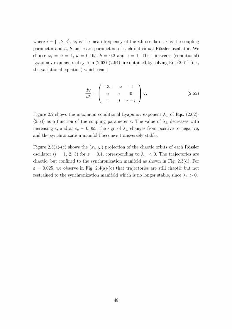
where i = 1, 2, 3, ωi is the mean frequency of the ith oscillator, ε is the coupling

parameter and a, b and c are parameters of each individual Rossler oscillator. We

choose ωi = ω = 1, a = 0.165, b = 0.2 and c = 1. The transverse (conditional)

Lyapunov exponents of system (2.62)-(2.64) are obtained by solving Eq. (2.61) (i.e.,

the variational equation) which reads

dv

dt=

−3ε −ω −1

ω a 0

z 0 x− c

v. (2.65)

Figure 2.2 shows the maximum conditional Lyapunov exponent λ⊥ of Eqs. (2.62)-

(2.64) as a function of the coupling parameter ε. The value of λ⊥ decreases with

increasing ε, and at εc ∼ 0.065, the sign of λ⊥ changes from positive to negative,

and the synchronization manifold becomes transversely stable.

Figure 2.3(a)-(c) shows the (xi, yi) projection of the chaotic orbits of each Rossler

oscillator (i = 1, 2, 3) for ε = 0.1, corresponding to λ⊥ < 0. The trajectories are

chaotic, but confined to the synchronization manifold as shown in Fig. 2.3(d). For

ε = 0.025, we observe in Fig. 2.4(a)-(c) that trajectories are still chaotic but not

restrained to the synchronization manifold which is no longer stable, since λ⊥ > 0.

48

-20 -10 0 10 20x

1

-20

-10

0

10

20y 1

Rossler 1

-20 -10 0 10 20x

2

-20

-10

0

10

20

y 2

Rossler 2

-20 -10 0 10 20X

3

-20

-10

0

10

20

y 3

Rossler 3

-20 -10 0 10 20x

1

-20

-10

0

10

20

x 2

(a) (b)

(c) (d)

FIGURE 2.3 - Projections of chaotic orbits for ε = 0.1 corresponding to (a) the firstcoupled Rossler oscillator, (b) the second coupled Rossler oscillator and (c)the second coupled Rossler oscillator. (d) The same orbit projected on the(x1, x2) plane.

-20 -10 0 10 20x

1

-20

-10

0

10

20

y 1

Rossler 1

-20 -10 0 10 20x

2

-20

-10

0

10

20

y 2

Rossler 2

-20 -10 0 10 20X

3

-20

-10

0

10

20

y 3

Rossler 3

-20 -10 0 10 20x

1

-20

-10

0

10

20

x 2

(a)

(c)

(b)

(d)

FIGURE 2.4 - Projections of chaotic orbits for ε = 0.025 of (a) the first coupled Rossleroscillator, (b) the second coupled Rossler oscillator and (c) the second cou-pled Rossler oscillator. (d) The same orbit projected on the (x1, x2) plane.

49

3 OBSERVATION OF SYNCHRONIZATION IN INTERMITTENT

TURBULENCE

In this Chapter, the techniques described in Section 2.1 are applied to two exam-

ples of intermittent turbulence observed in the solar-terrestrial environment: the

intermittent magnetic field turbulence observed in the solar wind using data from

satellites, in the solar photosphere using solar magnetograms and in the ground us-

ing magnetometers, and the intermittent atmospheric turbulence observed in the

Amazon rain forest canopy.

The solar wind provides a natural laboratory for observation of intermittent mag-

netic field turbulence (BRUNO; CARBONE, 2005; KAMIDE; CHIAN, 2007). Nonlinear

energy cascade (direct and inverse) due to multi-scale interactions leads to localized

regions of space plasmas where phase synchronization (phase coherence) involving a

finite degree of phase coupling among a number of active modes takes place. Large-

amplitude phase coherent structures seen in these localized regions dominate the

statistics of fluctuations at small scales and have typical lifetime longer than that of

incoherent (random-phase) fluctuations in the background.

A recent theoretical study of nonlinear waves shows that phase synchronization

associated with multi-scale interactions is the origin of bursts of coherent structures

in intermittent turbulence in plasmas and fluids (HE; CHIAN, 2003; HE; CHIAN, 2005).

Observational evidence in support of these findings in space plasma turbulence was

obtained by Hada et al. (2003), Koga and Hada (2003), Koga et al. (2007) and Koga

et al. (2008) using the Geotail solar wind data upstream and downstream of Earth’s

bow shock, by Sahraoui (2008) using the Cluster data in the magnetosheath close

to the Earth’s magnetopause, and by Telloni et al. (2009) using the SOHO data of

solar corona; and in atmospheric turbulence by Chian et al. (2008) using the Amazon

forest data.

Neutral fluid turbulence can be studied experimentally via measurements of the

Earth’s atmospheric turbulence such as the wind velocity or temperature fluctua-

tions. In the latter case, the Amazon rain forest plays a key role in the regional and

global climate dynamics. One important problem for understanding the vegetation-

atmosphere interactions in Amazonia is the turbulent exchange of scalar and mo-

mentum in the atmospheric boundary layer - above and within the forest canopy.

51

Atmospheric turbulence in the Amazon forest has been extensively investigated. For

example, Fitzjarrald et al. (1990) performed detailed observations of turbulence just

above and below the crown of an Amazon forest during the wet season. This analysis

shows that the forest canopy removes high-frequency turbulent fluctuations while

passing lower frequencies. A study of CO2 concentration was made by Sternberg et

al. (1997) in two different forests in the Amazon basin during the dry season, one site

characterized by a closed canopy structure in which turbulent mixing is minimized

and another site characterized by an open canopy structure in which the turbulent

mixing is maximized. This analysis shows that the respiratory CO2 recycling in the

closed canopy forest with lower wind speeds is occurring to a greater extent than

the open canopy forest with higher wind speeds. The vertical dispersion of trace

gases using a Lagrangian approach was analyzed by Simon et al. (2005) based on in-

canopy turbulence data collected at Jaru and Cuieiras Reserves. This study indicates

that for day-time conditions when there is an efficient turbulent mixing in the upper

canopy and profile gradients are small, the radon-222 source/sink distributions show

a high sensitivity to small measurement errors and the CO2 and H2O fluxes show

a reasonable agreement with the eddy covariance measurements made above the

forest canopy, which is not the case for night-time conditions when the CO2 profile

gradients in the upper canopy are large due to reduced turbulent mixing.

The remaining of this Chapter is divided as follows. Section 3.1 is devoted to the char-

acterization of intermittency and phase synchronization in intermittent magnetic

field turbulence. In particular, subsection 3.1.1 aims to seek further observational

evidence of phase synchronization in space plasmas based on the magnetic field data

of Cluster and ACE (Advanced Composition Explorer) spacecraft. We compare the

phase synchronization detected by Cluster in the magnetic field turbulence in the

shocked solar wind upstream of Earth’s bow shock with the phase synchronization

detected by ACE in the magnetic field turbulence in the unshocked ambient solar

wind at the L1 Lagrangian point. In subsection 3.1.2 we study the scale dependence

of kurtosis and phase coherence in intermittent magnetic field turbulence measured

at three different locations of the solar-terrestrial environment: (1) in the solar pho-

tosphere, (2) in the solar wind, and (3) on the ground. We investigate two scenarios:

a non-ICME event in February 2002 and an ICME event in January 2005. Section

3.2 aims to apply the kurtosis (fourth-order structure function) and phase coherence

techniques to determine the intermittent nature of day-time atmospheric turbulence

above and within the Amazon forest canopy. We show that both techniques are ca-

52

pable of characterizing the dissimilarity of scalar and velocity in above-canopy and

in-canopy atmospheric turbulence.

3.1 Synchronization in magnetic field turbulence

3.1.1 non-ICME event

The physical conditions upstream of Earth’s bow shock along the path of Cluster are

expected to differ from the unshocked ambient solar wind in the vicinity of ACE. The

magnetic connection between the interplanetary magnetic field (IMF) and the bow

shock may occur sporadically in the upstream solar wind, as evidenced by a strong

emission at the local electron plasma frequency (KELLOGG; HORBURY, 2005). In

contrast the ambient solar wind at L1, being far away from the Earth’s bow shock,

is not affected by the shock. This Section carries out a comparative study of the

degree of phase synchronization across a wide range of scales in the interplanetary

magnetic field fluctuations in shocked (Cluster) and unshocked (ACE) regions of

solar wind.

Cluster has observed intermittent interplanetary turbulence upstream of Earth’s

bow shock. The first study of solar wind intermittency using Cluster data was re-

ported by Pallocchia et al. (2002). They showed that velocity fluctuations detected

by Cluster-3 are slightly more intermittent than Cluster-1 on 22 February 2001. Bale

et al. (2005b) used the Cluster-4 data of 19 February 2002 to show that both electric-

field and magnetic-field fluctuations of turbulence in the upstream solar wind display

the k−5/3 spectral behavior of classical Kolmogorov fluid turbulence over an inertial

subrange and a spectral break at kρi ∼ 0.45 (where ρi is the ion Larmor radius). In

the dissipative subrange above the spectral break point, the magnetic spectrum be-

comes steeper while the electric spectrum gets enhanced. They suggest that Alfven

waves in the inertial subrange eventually disperse as kinetic Alfven waves above the

spectral break, becoming more electrostatic at short wavelengths where wave energy

is dissipated through wave-particle interaction processes such as Landau or tran-

sit time damping. Narita et al. (2006) determined directly the wavenumber power

spectra of intermittent magnetic field turbulence in the foreshock of a quasi-parallel

bow shock using four-point Cluster spacecraft measurements; they conjectured that

nonlinear interactions of Alfven waves can lead to phase coherence in the foreshock

turbulence observed by Cluster. Alexandrova et al. (2007) used the Cluster-1 data

of 5 April 2001 to demonstrate that in the inertial subrange below the ion cy-

53

clotron frequency, the turbulent spectrum of unshocked solar wind magnetic field

follows Kolmogorov’s law. However, after the spectral break the turbulence cannot

be characterized by a “dissipative” range. Instead, the kurtosis (fourth-order struc-

ture function) increases with frequency, similar to the intermittent behavior of the

low-frequency inertial subrange, indicating that nonlinear wave interactions are op-

erating to yield a new high-frequency inertial subrange. Alexandrova et al. (2008)

showed that the magnetic field fluctuations within the high-frequency inertial sub-

range identified by Alexandrova et al. (2007) is much more compressive than the

low-frequency inertial subrange dominated by incompressive Alfven waves. This in-

crease of compressibility is due to a partial dissipation (and destruction of phase

coherence) of left-hand Alfvenic fluctuations by the ion cyclotron damping in the

neighborhood of the spectral break point around the ion cyclotron frequency, leading

to a new right-hand “magnetosonic” small-scale cascade characterized by an increase

of intermittency as well as spectrum steepening.

ACE has monitored solar wind in an orbit about the L1 point. Burlaga and Vinas

(2004) showed that the fluctuations of solar wind speed observed by ACE are re-

lated to intermittent turbulence and shocks at the smallest scales (1 hour) and can

be described by a Tsallis probability distribution function derived from nonextensive

statistical mechanics. Smith et al. (2006) demonstrated that while the inertial sub-

range of solar wind magnetic field turbulence measured by ACE at lower frequencies

displays a tightly constrained range of spectral indexes, the dissipation range ex-

hibits a broad range of power-law indexes. Chapman and Hnat (2007) showed that

solar wind turbulence detected by ACE is dominated by Alfvenic fluctuations with

power spectral exponents that evolve toward the Kolmogorov value of - 5/3, and

can be decomposed into two coexistent components perpendicular and parallel to

the local average magnetic field. Hamilton et al. (2008) found that on average the

wave vectors of solar wind magnetic field turbulence measured by ACE are more

field-aligned in the dissipation subrange than in the inertial subrange, and cyclotron

damping plays an important but not exclusive role in the formation of the dissipa-

tion subrange; moreover, the orientation of the wave vectors for the smallest scales

within the inertial subrange are not organized by wind speed and that on average the

data shows the same distribution of energy between perpendicular and field-aligned

wave vectors.

Recently, a phase coherence technique for characterizing phase synchronization in

54

nonlinear wave-wave coupling and turbulence based on surrogate data has been de-

veloped for space plasmas (HADA et al., 2003; KOGA; HADA, 2003; KOGA et al., 2008;

SAHRAOUI, 2008). The link between phase coherence, non-Gaussianity and intermit-

tent turbulence was established by Koga et al. (2007), based on the Geotail magnetic

field data upstream and downstream of Earth’s bow shock. In this subsection, we

investigate phase synchronization due to nonlinear multiscale interactions and non-

Gaussian statistics using the magnetic field data collected by Cluster upstream of

Earth’s bow shock and by ACE in the ambient solar wind at L1. By applying the

phase coherence index technique to quantify the degree of phase synchronization,

we show that its variation with time scales is similar to kurtosis indicating a signifi-

cant departure from Gaussianity over a wide range of time scales, which is enhanced

at small scales, in agreement with the leptokurtic shape of small-scale probability

density function (PDF) of intermittent magnetic field fluctuations in both regions

of space plasmas.

3.1.1.1 Cluster and ACE data of 1 to 3 February 2002

Figure 3.1 depicts the orbit trace of Cluster and spacecraft position of ACE, in the

GSE Cartesian coordinate system, from 19:40:40 on 1 February 2002 to 03:56:38

on 3 February 2002 during which Cluster-1 traverses the upstream region of the

Earth’s bow shock. For this time interval, ACE appears practically stationary in

the scales of Figure 3.1 and the Cluster tetrahedron scale (i.e., the mean distance

between spacecrafts) was small (∼ 100-300 km). For spacecraft separations of 300

km and mean solar wind bulk velocity of 374 km/s (obtained for the selected time

interval) and assuming the Taylor’s hypothesis, the time scale above which all 4

Cluster spacecraft observe the same eddies is ∼ 0.8 s. In this study, our analysis

will cover time scales above 1 s (Figure 3.12), hence the differences of measurements

between the satellites are indistinguishable. The selected time interval, defined by

the onset of the solar wind supersonic/subsonic transitions, begins when Cluster-1

crosses the shock front of a quasi-perpendicular bow shock by entering into the solar

wind at the time indicated by a dashed line in the upper panel of Figure 3.2, and

ends when Cluster-1 departs from the solar wind by entering into the transition

(foreshock) region of a quasi-parallel bow shock at the time indicated by a dashed

line in the lower panel of Figure 3.2. In contrast to a quasi-perpendicular shock

(BALE et al., 2005a) characterized by sharp transitions of the modulus of the ion

bulk flow velocity |Vi| and magnetic field |B|, a quasi-parallel shock (BURGESS et

55

160240

0

080

40

80

−40

−80

GSE

GS

E

ACE

ER

RE

X ( )

Y

(

)

Cluster

FIGURE 3.1 - Orbit trace of Cluster and spacecraft position of ACE, in the GSE coor-dinate system, from 19:40:40 UT on 1 February 2002 to 03:56:38 UT on 3February 2002. The starting position of Cluster is shown as a full circle.

SOURCE: Chian and Miranda (2009)

al., 2005) is characterized by a transition region with repeated shock crossings, as

seen in Figure 3.2. This quasi-parallel shock event has been analyzed by a number of

papers (EASTWOOD et al., 2003; STASIEWICZ et al., 2003; BEHLKE et al., 2004; LUCEK

et al., 2004). When the Cluster spacecraft navigate in the upstream solar wind they

stay always very close to the bow shock, as a result magnetic connections to the bow

shock occur frequently (KELLOGG; HORBURY, 2005). Although we have selected an

interval outside of the foreshock region of a quasi-parallel bow shock the magnetic

connection happens from time to time, for example, between 00:50 and 01:00 UT,

and between 01:20 and 01:36 UT on 3 February 2002. Hence, the plasma conditions

of solar wind seen by Cluster-1 are different from that seen by ACE at L1 since the

solar wind turbulence measured by Cluster-1 is a combination of the ambient solar

wind plus fluctuations coming from the bow shock. Note that during the selected

56

0

100

200

300

400

500

0

100

200

300

400

500

0

10

20

30

40

0

10

20

30

40

19:25:40

03:41:38

Quasi−parallel shock crossing

Quasi−perpendicular shock crossing

19:40:40

03:56:38

Time (UT)

Day 32

Day 34

19:55:40

04:11:38

|B|

|B|

|V |

|V |i

i

FIGURE 3.2 - Cluster-1 magnetic field |B| (red, nT) and ion bulk flow velocity |Vi| (black,km/s) during the quasi-perpendicular shock crossing (upper panel) on Ju-lian day 32, 2002, and the quasi-parallel shock crossing (lower panel) onJulian day 34, 2002. The vertical dashed lines indicate the beginning andthe end of the selected time interval of Figure 3.4, respectively.


interval no M- or X-class solar flares were detected, as evidenced by the GOES-10 X-

ray data shown in Figure 3.3, and strong interplanetary disturbances such as ICMEs

were not seen.

In this study, we perform a nonlinear analysis of the modulus of magnetic field

|B| = (B2x +B2

y +B2z )

1/2. We are interested in analyzing the relation between phase

synchronization and intermittency of solar wind magnetic field turbulence which

does not require a detailed analysis of its field components. As a matter of fact, in a

similar study Bruno et al. (2003) showed that the modulus and the components of the

solar wind magnetic field give the same qualitative behaviors of intermittency. The

Cluster and ACE magnetic fields are detected by the FGM instruments (BALOGH et

al., 2001; SMITH et al., 1998) at a resolution of 22 Hz and 1 Hz, respectively, providing

a set of 2,604,208 and 116,159 data points, respectively, for the interval chosen. For

the sake of completeness, Figure 3.4 presents an overview of other in situ plasma

57

28 30 32 34 36Julian days of year 2002

10-9

10-8

10-7

10-6

10-5

10-4

10-3

Inte

nsity

(W

/m^2

)

X-Class event

M-Class event

1-8 A0.5-4 A

FIGURE 3.3 - GOES-10 X-ray fluxes from 28 January 2002 to 5 February 2002 (Julian day36). Red dashed lines indicates thresholds for X-class (10−4) and M-class(10−5− 10−4) events. None of the M-class X-ray events detected happenedduring the selected time interval.

parameters for this interval. The three components of the vector magnetic field Bx,

By and Bz are given in the GSE coordinates. ΦB and ΘB denote the angle of the

solar wind magnetic field relative to the Sun-Earth x-axis in the ecliptic plane, and

the angle out of the ecliptic, respectively, in the polar GSE coordinates (EASTWOOD

et al., 2003). These angles can be obtained from the following relations

ΦB = tan−1

(By

Bx

),

ΘB = tan−1

(Bz√

B2x +B2

y

).

Figure 3.4 also shows the modulus of the ion bulk flow velocity |Vi|, the ion number

density ni and the ion temperature Ti (where the component perpendicular to the

magnetic field for Cluster is plotted). It follows from Figure 3.4 that during this

time interval Cluster and ACE are immersed in a slow solar wind. The ion plasma

58

05

1015

20

-20-10

010

0

180

360

-90

0

90

300

360

420

0

20

40

104

106

0

10

20

Time (UT)

11:48:39Day 33

19:40:40 11:48:39Day 33

03:56:3803:56:38Day 34 Day 32 Day 34

19:40:40Day 32

|B|

nT

β

ACE

ΦB

ΘB

Cluster

ii

i|V

| iB

xB

yB

z

FIGURE 3.4 - ACE and Cluster-1 magnetic field and plasma parameters for the selectedtime interval. From top to bottom: modulus of magnetic field |B| (nT); thethree components of the vector magnetic field (nT) Bx, By, and Bz in theGSE coordinates; angle ΦB (degrees) of the magnetic field relative to thex axis in the ecliptic plane; angle ΘB (degrees) of the magnetic field outof the ecliptic; ion bulk flow velocity |Vi| (km/s), ion number density ni(cm−3), ion temperature Ti (Kelvin), and ion plasma beta βi.


59

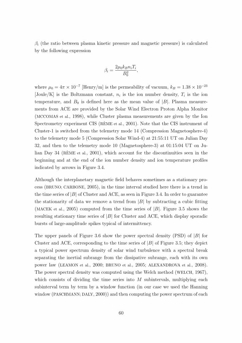
βi (the ratio between plasma kinetic pressure and magnetic pressure) is calculated

by the following expression

βi =2µ0kBniTi

B20

,

where µ0 = 4π × 10−7 [Henry/m] is the permeability of vacuum, kB = 1.38× 10−23

[Joule/K] is the Boltzmann constant, ni is the ion number density, Ti is the ion

temperature, and B0 is defined here as the mean value of |B|. Plasma measure-

ments from ACE are provided by the Solar Wind Electron Proton Alpha Monitor

(MCCOMAS et al., 1998), while Cluster plasma measurements are given by the Ion

Spectrometry experiment CIS (REME et al., 2001). Note that the CIS instrument of

Cluster-1 is switched from the telemetry mode 14 (Compression Magnetosphere-4)

to the telemetry mode 5 (Compression Solar Wind-4) at 21:55:11 UT on Julian Day

32, and then to the telemetry mode 10 (Magnetosphere-3) at 01:15:04 UT on Ju-

lian Day 34 (REME et al., 2001), which account for the discontinuities seen in the

beginning and at the end of the ion number density and ion temperature profiles

indicated by arrows in Figure 3.4.

Although the interplanetary magnetic field behaves sometimes as a stationary pro-

cess (BRUNO; CARBONE, 2005), in the time interval studied here there is a trend in

the time series of |B| of Cluster and ACE, as seen in Figure 3.4. In order to guarantee

the stationarity of data we remove a trend from |B| by subtracting a cubic fitting

(MACEK et al., 2005) computed from the time series of |B|. Figure 3.5 shows the

resulting stationary time series of |B| for Cluster and ACE, which display sporadic

bursts of large-amplitude spikes typical of intermittency.

The upper panels of Figure 3.6 show the power spectral density (PSD) of |B| for

Cluster and ACE, corresponding to the time series of |B| of Figure 3.5; they depict

a typical power spectrum density of solar wind turbulence with a spectral break

separating the inertial subrange from the dissipative subrange, each with its own

power law (LEAMON et al., 2000; BRUNO et al., 2005; ALEXANDROVA et al., 2008).

The power spectral density was computed using the Welch method (WELCH, 1967),

which consists of dividing the time series into M subintervals, multiplying each

subinterval term by term by a window function (in our case we used the Hanning

window (PASCHMANN; DALY, 2000)) and then computing the power spectrum of each

60

FIGURE 3.5 - Time series of the modulus of magnetic field |B| (nT) of Cluster-1 andACE, after removing the trend by computing a cubic fitting of the originaldata.


subinterval using the fast Fourier transform. The average of the M power spectra

gives the PSD. This method reduces the error of the spectrum estimate, resulting

in a narrower PSD. The spin frequency fspin of both spacecraft are indicated in

Figure 3.6. The Nyquist frequency fNyq, defined as half of the sampling frequency

fs, fNyq = 0.5fs, which marks the maximum frequency for which the PSD gives

reliable values (PASCHMANN; DALY, 2000), is equal to 11 Hz for Cluster and 0.5 Hz

for ACE.

The frequency range in which each PSD follows a −5/3 Kolmogorov scaling (i.e.,

the inertial subrange) can be determined by constructing the compensated PSD,

multiplying the original PSD by f+5/3 (BISKAMP et al., 1999). The inertial subrange

should appear as a frequency range in which the compensated PSD is almost hori-

zontal (i.e., zero slope). The compensated PSD of Cluster and ACE are shown in the

lower panels of Figure 3.6. To facilitate visualization, each compensated spectrum

is smoothed by dividing it into overlapping subintervals shifted by one datapoint,

each subinterval contains 10 datapoints, and then calculating the mean value within

61

10-6

10-4

10-2

100

102

104

10-3

10-2

10-1

100

10110

-4

10-3

10-2

10-1

10-3

10-2

10-1

100

101

PSD

(nT

/H

z)2

fspin

fNyq

fspin

f (Hz)(Hz)f

PSD

5/3

f

Cluster ACE

−1.6

−2.1

−1.5

−2.0

FIGURE 3.6 - Upper panels: Power spectral density (PSD) of |B| for Cluster-1 and ACE.The spin frequency of each spacecraft is indicated as fspin. The Nyquistfrequency for ACE is indicated as fNyq. Straight lines indicate the inertialand “dissipative” subranges of each spacecraft. The spectral break thatmarks the transition from the inertial to dissipative subrange occurs nearthe local ion cyclotron frequency fci. For both Cluster and ACE fci ∼ 0.12Hz in the solar wind frame, which is Doppler-shifted to a higher frequencyin the spacecraft frame. Lower panels: Compensated PSD for Cluster andACE. To facilitate visualization, a smoothed compensated PSD is shownin black. Vertical dashed lines indicate the beginning and the end of theinertial subranges used to compute the spectral indices of Cluster and ACEin the upper panels.


62

10-3

10-2

10-1

100

10110

-6

10-4

10-2

100

102

104

10-3

10-2

10-1

100

101

PS

D(n

T /H

z)2

(Hz)f f (Hz)

Cluster ACE

FIGURE 3.7 - Power spectral density of |B| for Cluster-1 and ACE. Black curves indicatethe upper and lower bounds of confidence intervals (error bars).

each subinterval. Each mean value is plotted at the center of the subinterval. The

smoothed compensated spectra of Cluster and ACE are shown in the lower panels of

Figure 3.6 (black curves), and the vertical dashed lines indicate the beginning and

the end of the resulting inertial subrange. For both Cluster and ACE, the beginning

of the inertial subrange is defined as the first value of the smoothed compensated

PSD. For Cluster, the compensated spectrum clearly shows a “knee” (i.e., a local

maximum) to the right of fspin, hence the end of the inertial subrange is defined as

the frequency just before the “knee”. For ACE, the end of the inertial subrange is

defined as the frequency where a change of slope occurs. For Cluster, the inertial

subrange spectral index in the frequency range 0.0026-0.3 Hz is qinert = −1.6± 0.01

and the dissipative subrange spectral index in the frequency range 0.6-3.74 Hz is

qdissip = −2.1± 0.01. For ACE, the inertial subrange spectral index in the frequency

range 0.0013-0.1 Hz is qinert = −1.5 ± 0.01 and the dissipative subrange spectral

index in the frequency range 0.18-0.33 Hz is qdissip = −2.0± 0.04.

The fluctuations of the modulus of magnetic field |B| can be regarded as compressible

(or parallel) fluctuations (SAMSONOV et al., 2007; ALEXANDROVA et al., 2008). The

total power spectral density PSDtotal is closer to the −5/3 Kolmogorov scaling than

the PSD of |B| (PSD‖), where PSDtotal = PSD(Bx)+PSD(By)+PSD(Bz) = PSD⊥+

PSD‖, PSD⊥ denotes the PSD of transverse Alfvenic fluctuations (SAMSONOV et al.,

2007). In the solar wind at 1 AU, magnetic field fluctuations are mostly Alfvenic and

nearly incompressible (ALEXANDROVA, 2008) which implies that, within the inertial

63

subrange, transverse fluctuations contain more power than compressible fluctuations.

For the sake of completeness, we calculated the standard deviation resulting from

averaging a set of power spectra, after applying the Welch method. The standard

deviation of each frequency, also called the confidence intervals, are represented as

black curves in Figure 3.7, superposed by the PSDs of Cluster and ACE.

The spectral break that marks the transition from the inertial to dissipative subrange

occurs near the local ion cyclotron frequency fci = eB/mi in an appropriate frame.

For both Cluster and ACE fci ∼ 0.12 Hz if we use B0 in the solar wind frame.

Since data are taken in the spacecraft frame, fci has to be Doppler-shifted to higher

frequency by a quantity of the order of Vsw/VA, where Vsw is the solar wind speed

and VA is the Alfven speed, in the interpretation of the power spectra in Figure 3.6.

3.1.1.2 Intermittency, non-Gaussianity and phase synchronization

Figure 3.8 shows the scale dependence of the normalized magnetic field-differences

of Cluster and ACE

∆B =δB − 〈δB〉

σB, (3.1)

for three different time scales (τ = 10 s, 100 s and 1000 s), where δB = |B(t+ τ)| −|B(t)| denotes two-point differences of the modulus of magnetic field |B| for a given

time scale (lag) τ , the brackets denote the mean value of δB, and σB denotes the

standard deviation of δB. It is evident from Figure 3.8 that, for both Cluster and

ACE, the magnetic field fluctuations become more intermittent as the scales become

smaller. In terms of spatial scales, the three time scales in Figure 3.8 correspond to

3,740 km, 37,400 km and 374,000 km, respectively, using the mean solar wind (ion

bulk flow) velocity of 374 km/s and assuming the Taylor’s hypothesis. Note that the

spin frequency is filtered from the time series of Cluster and ACE, respectively, by

applying an orthogonal wavelet decomposition to the data using a Daubechies 10

mother wavelet (DAUBECHIES, 1994), and removing the scales corresponding to the

spacecraft spintone of 0.25 Hz for Cluster and 0.083 Hz for ACE.

The intermittent characteristics of interplanetary turbulence can be elucidated by

the probability density function (PDF) of magnetic field fluctuations. The p-th order

of the structure function is formally defined as (DE WIT, 2004)

64

B∆

B∆

Time (UT)

ACE

Cluster

22:59:00Day 33

sτ = 10

sτ = 100

sτ = 10

τ = 1000s

τ = 1000s

τ = 100 s

23:09:30

22:59:00Day 33

23:09:30

23:20:00

23:20:00

FIGURE 3.8 - Scale dependence of the normalized magnetic field-differences of Cluster(red) and ACE (blue) for three different time scales (τ = 10 s, 100 s and1000 s).


Sp(τ) =

∫ ∞−∞

P (∆B(τ))(∆B(τ))pd(∆B(τ)), (3.2)

where P (∆B) denotes the probability density function (PDF) of magnetic field dif-

ferences ∆B. The first four orders of the structure function are statistical quantities

that characterize PDFs (PAPOULIS, 1965; DAVIDSON, 2004), namely, p = 0 gives the

sum of all probabilities (equal to 1 by definition), p = 1 gives the mean value of

∆B (equal to zero according to Eq. 3.1), p = 2 gives the variance of ∆B (equal to

1 from Eq. 3.1, whose square root is the standard deviation), p = 3 measures the

degree of asymmetry (skewness) of the distribution, and p = 4 quantifies the flatness

of the distribution. Figure 3.9 plots the integrand of Eq. (3.2) for p = 0 (PDF) and

4 (flatness), determined from the magnetic field fluctuations of Cluster and ACE

65

TABLE 3.1 - Numerical examples of flatness for three time scales

τ = 10 s 100 s 1000 s

Cluster 35.86 14.41 6.80

ACE 47.39 16.02 7.67

(Figure 3.5), for 3 different time scales (τ = 10 s, 100 s and 1000 s), superposed

by a Gaussian PDF (grey line). It shows that the PDFs of ∆B for both shocked

and unshocked solar wind are closer to a Gaussian distribution at large time scales

but deviate from a Gaussian distribution as τ decreases. At small scales the shape

of PDF (p = 0) becomes leptokurtic, exhibiting fat tails and sharp peaks. For p

= 4, the flatness of the distribution of ∆B of both Cluster and ACE increases at

small scales, indicating an excess of rare, large-amplitude fluctuations. The areas

spanned by the curves shown in Figure 3.9 for p = 4 approximate the values of the

fourth-order (flatness) structure function (DE WIT, 2004). Table 3.1 lists numerical

examples of flatness which shows that, for all three scales, the level of flatness of

magnetic field fluctuations of ACE is higher than Cluster.

The departure from self-similarity in the magnetic field fluctuations can be quantified

by comparing the scaling exponents of higher-order structure functions within the

inertial subrange against the Kolmogorov universality theory (FRISCH, 1995). The

characterization of departures from Kolmogorov’s 1941 theory (hereafter K41) is

of great interest since the K41 theory is a result based on the assumption that

the turbulence is homogeneous and isotropic (i.e., self-similar). The upper panels of

Figure 3.10 show the structure functions obtained from the following formula (DE

WIT; KRASNOSELSKIKH, 1996),

Sp(τ) = 〈|Bi+τ −Bi|p〉 ∼ τα(p), (3.3)

for p = 1 - 6. The scale is logarithmic for both axes. The grey areas denote the inertial

subranges determined from the power spectral density of Figure 3.6. The scaling

66

10-6

10-3

100

103

Cluster

ACE

10-6

10-3

100

103

-30 -20 -10 0 10 20 3010

-6

10-3

100

103

10-6

10-3

100

103

10-6

10-3

100

103

-30 -20 -10 0 10 20 3010

-6

10-3

100

103

P(∆

B)(∆

B)p

P(∆

B)(∆

B)p

P(∆

B)(∆

B)p

∆B∆B

τ = 100 τ = 100s s

p = 0

τ = 10 s τ = 10 s

τ = 1000 sτ = 1000 s

p = 4

FIGURE 3.9 - The integrand of Equation 3.2, for p = 0 and p = 4, determined fromthe magnetic field fluctuations of Cluster-1 (red) and ACE (blue), for threedifferent time scales (τ = 10 s, 100 s and 1000 s), superposed by a GaussianPDF (grey line). The areas spanned by the curves of Cluster and ACE forp = 4 approximate the value of the flatness.


67

FIGURE 3.10 - Upper panels: variations of structure functions with timescale τ calculatedfrom the magnetic field fluctuations of Cluster-1 and ACE (upper panels)for p = 1 (black), 2 (purple), 3 (light green), 4 (yellow), 5 (dark green)and 6 (light blue), the grey area indicates the inertial subrange. Lowerpanels: structure functions after applying the Extended Self-Similaritytechnique, the bar indicates the previous inertial subrange, and the greyarea indicates the extended scaling range. For the visualization purpose,the stretched structure functions have been normalized to Sp(T ), whereT = 0.044 s for Cluster and T = 1 s for ACE.


68

exponent for each order of the structure function can be obtained by estimating the

slope of a linear-fit of the curves within the inertial subrange. In order to improve

the calculation of the scaling exponent, we apply the Extended Self-Similarity (ESS)

technique (BENZI et al., 1993), which consists of plotting each order of the structure

function Sp as a function of S3. This technique allows us to extend the scaling range

where Sp(τ) ∼ [S3(τ)]ζ(p). The scaling exponents ζ(p) ∼ α(p)/α(3) can be found

from the extended range. The lower panels of Figure 3.10 illustrate the application

of this technique. The horizontal line represents the inertial subrange before the

“stretching” process, and the grey area indicates the extended scaling range. Figure

3.11 shows the scaling exponent ζ(p) as a function of p, for Cluster and ACE. The

dashed line denotes the K41 scaling, ζ(p) = p/3. It is evident, from Figure 3.11, that

the scaling exponent measured by both spacecraft display significant departure from

self-similarity, which implies that the magnetic field fluctuations in both regions of

space plasmas are intermittent. For the time interval considered in this work, the

unshocked solar wind magnetic field at L1 is more intermittent than the shocked

solar wind upstream of Earth’s bow shock, in agreement with Table 1.

Intermittency can be quantified by calculating the empirical estimate of the normal-

ized fourth-order moment K (kurtosis) (DE WIT, 2004),

K(τ) =1

n

n∑i=1

(δBi − 〈δBi〉

σB

)4

− 3, (3.4)

which is equivalent to flatness minus 3 (FRISCH, 1995; DAVIDSON, 2004). For a

Gaussian noise K = 0 for all scales; whereas for an intermittent (non-Gaussian)

signal K(τ) > 0 and K increases as scale decreases within the inertial subrange.

Figure 3.12 shows the computed variation of K with the time scale τ for magnetic

field fluctuations of Cluster and ACE. We have chosen the lower bound of 1 s for

Figure 3.12 since the measurements at scales smaller than 1 s are contaminated by

the noise level of FGM instruments. The test to find the smallest time scale is done

by over-plotting the instrument noise level of 10−4 nT2/Hz (for both Cluster and

ACE) on the power spectral density of Figure 3.6.

An alternative method of quantifying intermittency and non-Gaussianity is to apply

the phase coherence technique using surrogate data by defining a phase coherence

index (HADA et al., 2003; KOGA; HADA, 2003; KOGA et al., 2007; KOGA et al., 2008;

69

1 2 3 4 5 6

0.5

1

1.5

2

K41ClusterACE

(p)

ζ

p

FIGURE 3.11 - Scaling exponent ζ of the p-th order structure function obtained by ESSfitting for Cluster-1 and ACE magnetic field fluctuations. The dashed linecorresponds to K41 (self-similar) Kolmogorov scaling.


NARIYUKI; HADA, 2006; CHIAN et al., 2008; NARIYUKI et al., 2008; SAHRAOUI, 2008;

TELLONI et al., 2009)

Cφ(τ) =SPRS(τ)− SORG(τ)

SPRS(τ)− SPCS(τ), (3.5)

where

Sj(τ) =n∑i=1

|Bi+τ −Bi|, (3.6)

with j = ORG, PRS, PCS. This index measures the degree of phase synchronization

in an original data set (ORG) by comparing it with two surrogate data sets created

from the original data set: a phase-randomized surrogate (PRS) in which the phases

of the Fourier modes are made completely random, and a phase-correlated surrogate

70

0

50

100Cluster

ACE

| |

| |

100

101

102

103

104

0

0.5

1

τ (sec)

Ph

ase

Co

her

ence

In

dex

Ku

rto

sis

cb

a

FIGURE 3.12 - Kurtosis and phase coherence index of |B| measured by Cluster-1 (red)and ACE (blue). Letters a, b and c indicate scales τ = 10, 100 and 1000s, respectively. The bars indicate the inertial subrange of each spacecraftobtained from Figure 3.6. The inverse of the ion cyclotron frequency fci ∼0.12 Hz in the solar wind frame is τ ∼ 8.3 sec, which is near the peakregions of kurtosis and phase coherence index.


(PCS) in which the phases of the Fourier modes are made completely equal. The

power spectrum of three data sets ORG, PRS and PCS are kept the same, but their

phase spectra are different. An average of over 100 realizations of the phase shuffling

is performed to generate the phase-randomized surrogate data set SPRS(τ). Cφ(τ)=0

indicates that the phases of the scales τ of the original data are completely random

(i.e., null phase synchronization), whereas Cφ(τ)=1 indicates that the phases are

fully correlated (i.e., total phase synchronization). Figure 3.12 displays the computed

variation of Cφ with the time scale τ for magnetic field fluctuations of Cluster and

ACE, whose behaviors follow that of kurtosis.

The upper panel of Figure 3.12 shows the variation of kurtosis as a function of the

time scale τ . For large scales (τ>∼ 103 sec) kurtosis is nearly zero, implying that the

magnetic field fluctuations are near-Gaussian (phase incoherent). For 10 sec<∼ τ

<∼103 sec, kurtosis increases as the time scale decreases which characterizes intermit-

71

tency and non-Gaussianity related to nonlinear energy cascade within the inertial

subrange seen in Figure 3.6. The lower panel of Figure 3.12 shows the variation of

the phase coherence index with τ which presents similar characteristics of kurtosis,

indicating that phase synchronization due to nonlinear multi-scale interactions is

responsible for intermittency. The inertial subranges for Cluster and ACE (obtained

from Figure 3.6) are marked with a bar in Figure 3.12. The results of Figure 3.12

display similar trend as the upstream results of Koga et al. (2007) obtained by the

Geotail data at the Earth’s bow shock in the sense that, as the scale τ decreases,

both kurtosis and phase coherence index increase until a certain scale where they

reach their respective maxima, and then both kurtosis and phase coherence index

start to decrease as τ decreases.

We conclude from Figure 3.12 that either kurtosis or phase coherence index can be

used to determine the degree of intermittency and phase synchronization in solar

wind turbulence. Both nonlinear techniques prove that the solar wind magnetic

field fluctuations, measured by Cluster and ACE, are intermittent (non-Gaussian)

exhibiting high degree of intermittency (non-Gaussianity) at small scales and low

degree of intermittency (near-Gaussianity) at large scales, in complete agreement

with Figures 3.8-3.11. It is interesting to point out that the period of 10 s of Alfven

waves analyzed by Eastwood et al. (2003) in the same Cluster event, from 04:02:30

UT to 04:10:00 UT (outside of our interval), is close to the peak of Figure 3.12 where

the intermittency is strongest. In addition, solar wind turbulence can be decomposed

into coherent (non-Gaussian) and incoherent (Gaussian) component using the local

intermittent measure analysis (ALEXANDROVA et al., 2008).

3.1.2 ICME event

In this subsection we study the scale dependence of kurtosis and phase coherence in

intermittent magnetic field turbulence measured at three different locations of the

solar-terrestrial environment: (1) in the solar photosphere, (2) in the solar wind, and

(3) on the ground. We perform a comparison of two scenarios: a non-ICME event in

February 2002 and an ICME event in January 2005.

72

0

2

4

6

8

Kur

tosi

s

AR 09802Quiet region

100

101

102

r (× 1.45 Mm)

0

0.5

1

Phas

e C

oher

ence

Ind

ex

(a) (b)

SOHO MDI solar image at 22:24 UT on 1 February 2002

FIGURE 3.13 - (a) SOHO MDI solar image taken at 22:24 UT on 1 February 2002. Thetwo white squares enclose two areas containing the active region AR 09802(upper), and a quiet region (lower). (b) Kurtosis (upper panel) and thephase coherence index (lower panel) as a function of spatial scale r com-puted from AR 09802 and the quiet region.

SOURCE: Miranda et al. (2009)

0

2

4

6

8

Kur

tosi

s


100

101

102

r (× 1.45 Mm)

0

0.5

1

Phas

e C

oher

ence

Ind

ex

SOHO MDI solar image at 04:47 UT on 16 January 2005

(a) (b)

FIGURE 3.14 - (a) SOHO MDI solar image taken at 04:47 UT on 16 January 2005. Thetwo white squares enclose two areas containing the active region AR 10720(upper), and a quiet region (lower). (b) Kurtosis (upper panel) and thephase coherence index (lower panel) as a function of spatial scale r com-puted from AR 10720 and the quiet region.


73

3.1.2.1 Non-Gaussianity and phase synchronization in the solar-

terrestrial environment

Solar images obtained by the SOHO MDI instrument provide the measurement of

the magnetic field in the solar photosphere. Near the centre of the solar image the

projection effects are negligible, hence the MDI solar image represents the vertical

or line-of-sight component of the photospheric magnetic field B‖ (ABRAMENKO et

al., 2002). Figure 3.13(a) shows a solar magnetogram taken by SOHO MDI on 1

February 2002. The white color corresponds to positive magnetic polarity, and the

black color corresponds to negative magnetic polarity. The two white squares mark

two selected areas, one containing the active region AR 09802 (upper) and the

other containing a quiet region (lower). Figure 3.13(b) shows kurtosis and the phase

coherence index as a function of spatial scale r computed from the two selected

regions. From Figure 3.13(b) we observe that the variation of kurtosis with r in the

quiet region is close to a Gaussian process (K = 0), being scale-invariant for all scales

r>∼2 pixels ∼ 2.9 megametres (Mm), consistent with the features of a monofractal

process (ABRAMENKO et al., 2002). The active region, on the other hand, displays

an increase of kurtosis as the spatial scale r decreases, which is a characteristic

of a non-Gaussian process related to nonlinear energy cascade within the inertial

subrange, and these values are higher than those obtained from the quiet region for

scales<∼20 pixels ∼ 29 Mm. The degree of phase synchronization measured by the

phase coherence index (HADA et al., 2003; KOGA et al., 2007; CHIAN; MIRANDA, 2009)

in the active region increases with decreasing spatial scale r, while the quiet region

presents low-degree of synchronization at all scales. Note that at large scales the

lack of datapoints introduces big errors in the computation of the phase coherence

index.

Figure 3.14(a) shows a SOHO MDI solar magnetogram obtained on 16 January 2005.

The two white squares enclose two selected areas containing the active region AR

10720 (upper) and a quiet region (lower), respectively. On 19-20 January 2005 several

flares associated with CMEs were observed in AR 10720, however in this period the

active region is too close to the solar limb, and the projection effects cannot be

neglected. Hence, we restrict our analysis to this earlier solar image when AR 10720

is near the disk centre. Figure 3.14(b) shows kurtosis and the phase coherence index

as a function of spatial scale r. It shows that the kurtosis of AR 10720 increases as

the scale r decreases, while kurtosis of the quiet region displays scale-invariance for

74

all scales r>∼2 pixels ∼ 2.9 Mm, similar to Fig. 3.13(b). Likewise, the phase coherence

index in Fig. 3.14(b) presents similar behavior as Fig. 3.13(b).

Now we direct our attention to the interplanetary magnetic field data collected

in situ in the solar wind. Figure 3.15(a) shows the time series of the modulus of

magnetic field |B| obtained by ACE and Cluster from 19:40:40 UT on 1 February

2002 to 03:56:38 UT on 3 February 2002. During this interval Cluster is in the

solar wind upstream of the Earth’s bow shock (CHIAN; MIRANDA, 2009). Although

Fig. 3.13(a) indicates the presence of several solar active regions on 1 February

2002, no M- or X-class solar flares occurred during the selected interval, and strong

interplanetary disturbances such as ICMEs were not seen. The upper panel of Figure

3.15(b) shows the variation of kurtosis as a function of time scale τ for magnetic field

fluctuations of ACE and Cluster. For 10 s<∼ τ

<∼ 103 s, kurtosis increases as the time

scale decreases, which characterizes non-Gaussianity. The lower panel of Fig. 3.15(b)

shows the variation of the phase coherence index with τ which presents a behavior

similar to kurtosis. From Fig. 3.15(b) we observe that the behavior of kurtosis and

the phase coherence index detected by ACE and Cluster are very similar except for

scales around 10 s, where ACE observes a higher level of intermittency and phase

synchronization than Cluster.

Figure 3.16(a) shows the time series of the modulus of magnetic field |B| measured

by ACE for the ICME event of 21-22 January 2005 (FOULLON et al., 2007). We se-

lected two intervals from this event. The first interval is located upstream of the

ICME shock which begins at 06:00:00 UT on 21 January and ends at 16:00:00 UT

on 21 January. The second interval is located downstream of the ICME shock which

begins at 16:47:19 UT on 21 January, and ends at 21:20:00 UT on 22 January.

Arrows indicate the selected intervals in Figure 3.16(a). In order to ensure the sta-

tionarity of data we avoid the “foot” transition region associated with the ICME

shock front. Figure 3.16(b) shows kurtosis and the phase coherence index as a func-

tion of time scale τ computed from the modulus of magnetic field |B| in upstream

and downstream regions of the ICME shock. It is evident, from Figure 3.16(b), that

both upstream and downstream regions indicate the features of intermittency and

phase synchronization across scales; moreover, the level of intermittency and phase

synchronization are higher in the downstream region than the upstream region for

all scales τ .

We analyze next the Earth’s geomagnetic field data obtained from two ground mag-

75

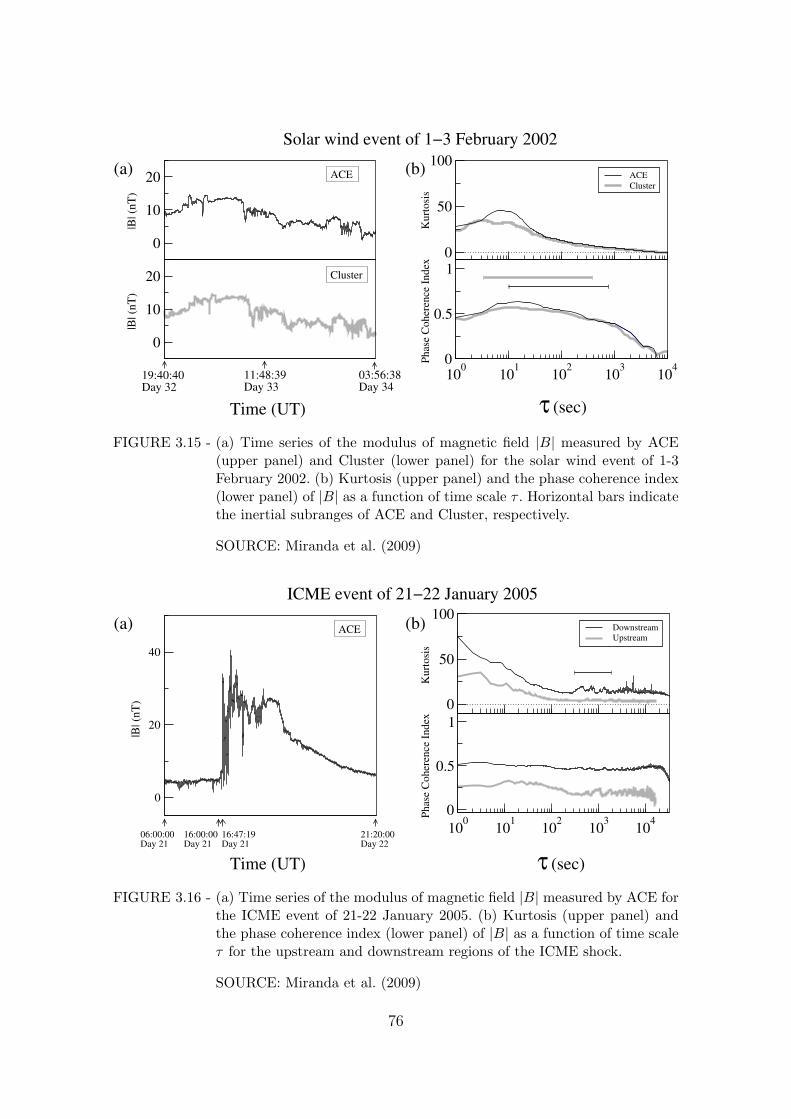
0

10

20

0

10

20

19:40:40Day 32

11:48:39Day 33

03:56:38Day 34

0

50

100ACE

Cluster

| |

| |

100

101

102

103

104

0

0.5

1

ACE(a)

|B| (

nT

)|B

| (nT

)

Time (UT)

Cluster

τ (sec)

(b)

Ph

ase

Co

her

ence

In

dex

Ku

rto

sis

Solar wind event of 1−3 February 2002

FIGURE 3.15 - (a) Time series of the modulus of magnetic field |B| measured by ACE(upper panel) and Cluster (lower panel) for the solar wind event of 1-3February 2002. (b) Kurtosis (upper panel) and the phase coherence index(lower panel) of |B| as a function of time scale τ . Horizontal bars indicatethe inertial subranges of ACE and Cluster, respectively.


| |

0

50

100Downstream

Upstream

100

101

102

103

104

0

0.5

1

0

20

40

06:00:00Day 21

16:00:00Day 21

16:47:19Day 21

21:20:00Day 22

τ (sec)

ACE (b)

ICME event of 21−22 January 2005

|B| (

nT

)

(a)

Time (UT)

Ku

rto

sis

Ph

ase

Co

her

ence

In

dex

FIGURE 3.16 - (a) Time series of the modulus of magnetic field |B| measured by ACE forthe ICME event of 21-22 January 2005. (b) Kurtosis (upper panel) andthe phase coherence index (lower panel) of |B| as a function of time scaleτ for the upstream and downstream regions of the ICME shock.


76

0

5

10

15

20

|B| (

nT)

-200

0

200

400

|B| (

nT)

-2

0

2

Pc3

-2

0

2

Pc4

-20

0

20

Pc5

0

50

100

Kur

tosi

s

ACEJPA

100

101

102

103

104

0

0.5

1

Pha

se C

oher

ence

Inde

x

Ground magnetometer data at Ji-Parana (JPA), Brazil(Geomagnetic latitude: ~ 0

o)

Time (UT)

19:40:40Day 32

11:48:39Day 33

03:56:38Day 34

τ (sec)

ACE

JPA

´

FIGURE 3.17 - (a) From top to bottom: time series of |B| measured by ACE for the solarwind event of 1-3 February 2002; modulus of the Earth’s geomagnetic field|B| measured by a ground magnetometer at Ji-Parana, Brazil, during thesame time interval; time series of Pc3 (10-45 s), Pc4 (45-150 s) and Pc5(150-1000 s) micropulsations. (b) Kurtosis (upper panel) and the phasecoherence index (lower panel) of |B| measured by ACE and the groundmagnetometer at JPA as a function of time scale τ.


0

20

40

|B| (

nT)

-200

0

200

|B| (

nT)

-15

0

15

Pc3

-15

0

15

Pc4

-15

0

15

Pc5

06:00:00Day 21

21:20:00Day 22

16:00:00Day 21

16:47:19Day 21

| |

0

10

20

Kur

tosi

s

VSS DownstreamVSS Upstream

100

101

102

103

104

0

0.5

1

Phas

e C

oher

ence

Ind

ex

Ground magnetometer data at Vassouras (VSS), Brazil(Geomagnetic latitude: ~ 19

o)

Time (UT) τ (sec)

ACE

VSS

FIGURE 3.18 - (a) From top to bottom: time series of |B| (nT) measured by ACE for theICME event of 21-22 January 2005; modulus of the Earth’s geomagneticfield |B| (nT) measured by a ground magnetometer at Vassouras, Brazil;time series of Pc3 (10-45 s), Pc4 (45-150 s) and Pc5 (150-1000 s) micropul-sations. (b) Kurtosis (upper panel) and the phase coherence index (lowerpanel) of |B| measured by the ground magnetometer at VSS as a functionof time scale τ .


77

netometers. The top panel of Fig. 3.17(a) shows the time series of the modulus of

magnetic field |B| observed by ACE at L1 during the non-ICME solar wind event of

1-3 February 2002. The second panel shows the modulus of the Earth’s geomagnetic

field measured by a ground magnetometer at Ji-Parana (JPA), Brazil (geomagnetic

latitude ∼ 0o). The three bottom panels show the time series of Pc3 (10-45 s), Pc4

(45-150 s) and Pc5 (150-1000 s) continuous geomagnetic pulsations, respectively.

Each time series of geomagnetic micropulsations is obtained by applying a Fourier

band-pass filter. Fig. 3.17(b) shows kurtosis and the phase coherence index of ACE

magnetic field data and JPA geomagnetic field data as a function of time scale τ . Fig.

3.17(b) indicates that the geomagnetic field fluctuations measured on the ground are

intermittent. For almost all scales the level of intermittency and phase coherence of

ACE are higher than the JPA.

Finally, for the ICME event of 21-22 January 2005, we plot in the top panel of

Figure 3.18(a) the time series of the modulus of magnetic field |B| observed by ACE

and in the second panel the modulus of the Earth’s geomagnetic field measured by

a ground magnetometer at Vassouras (VSS), Brazil (geomagnetic latitude ∼ 19o).

The three bottom panels show the time series of Pc3, Pc4 and Pc5 geomagnetic

micropulsations. All the time series of VSS were shifted by −1462 s to synchronize

with the ICME shock arrival at ACE. After shifting, we divide the VSS geomagnetic

field time series into“upstream”and“downstream”intervals in analogy with the ACE

magnetic field data of the ICME shock. Figure 3.18(b) shows kurtosis and the phase

coherence index of the VSS upstream and downstream intervals as a function of time

scale τ . It shows that for all scales the level of intermittency and phase coherence are

higher in the “downstream” geomagnetic field-fluctuations after the arrival of ICME

than the “upstream” geomagnetic field fluctuations before the arrival of ICME.

A comparison of the variation of kurtosis and the phase coherence index as a function

of τ for the downstream intervals observed by ACE in the solar wind (Fig. 3.16(b))

and the VSS ground magnetometer (Fig. 3.18(b)) reveals a common feature consist-

ing of three peaks between scales τ ∼ 304 s and τ ∼ 1860 s, marked with a bar in

both figures. This can be interpreted as evidence of a close correlation of the Earth’s

geomagnetic field with the ICME driver at these scales.

78

3.2 Synchronization in atmospheric turbulence

The aim of this section is to apply the kurtosis (fourth-order structure function)

and phase coherence techniques to determine the intermittent nature of day-time

atmospheric turbulence above and within the Amazon forest canopy. In particular,

we show that both techniques are capable of characterizing the dissimilarity of scalar

and velocity in above-canopy and in-canopy atmospheric turbulence.

3.2.1 Amazon forest canopy data

A major atmospheric mesoscale campaign during the wet season of the Large-Scale

Biosphere-Atmosphere Experiment in Amazonia (LBA) was carried out in January-

March 1999 (SILVA DIAS et al., 2002). LBA is an international project led by Brazil

designed to study: 1) the climatological, ecological, biogeochemical, and hydrological

functions of the Amazon region, 2) the impact of land uses caused by deforestation,

and 3) the interactions between Amazonia and the Earth system. As part of this

campaign, a micrometeorological tower was set up in a southwest Amazon basin at

the Biological Reserve of Jaru (Rebio Jaru: 1004’S, 6156’W) in Rondonia State

of Brazil; with instruments located at two different heights: above-canopy at 66 m

and inside-canopy at 21 m, to make simultaneous measurements of eddy covari-

ance and vertical profiles of air temperature, wind velocity, radiation and humidity.

Three-dimensional wind velocity and air temperature measurements were made at

a sampling rate of 60 Hz, using sonic anemometers and thermometers.

In this section we investigate the atmospheric turbulence data taken from noon to

12:30 on Julian Day 068, when the forest crown is heated by the solar radiation.

A dataset of 108000 points for temperature and vertical velocity is used for this

analysis. During this period the top of the canopy is hotter than its surroundings,

thus temperatures decrease both upwards towards the atmosphere above the canopy

and downwards towards the ground surface, resulting in an unstably stratified atmo-

sphere above the canopy and a stably stratification region inside the canopy. Figure

3.19 shows the original time series of temperature T and vertical wind velocity w

above and within the Amazon forest canopy.

3.2.2 Intermittency and phase coherence in atmospheric turbulence

Figures 3.20 and 3.21 show, respectively, the scale dependence of the normalized

temperature-difference ∆T = (δT− < δT >)/σT and the normalized vertical wind

79

12:00:00 12:15:00 12:30:00-2

-1

0

1

2

12:00:00 12:15:00 12:30:0028

28.2

28.4

28.6

28.8

29

12:00:00 12:15:00 12:30:0028

28.2

28.4

28.6

28.8

29

12:00:00 12:15:00 12:30:00-2

-1

0

1

2

T (

C)

o

ABOVE−CANOPY IN−CANOPY

Local Time

Local Time Local Time

Local Time

T (

C)

o

w (

m/s

)

w (

m/s

)

FIGURE 3.19 - Time series of temperature T and vertical wind velocity w above theAmazon forest canopy (left panels) and within the Amazon canopy (rightpanels), taken from noon to 12:30 on Julian Day 068, 1999.

SOURCE: Chian et al. (2008)

velocity-difference ∆w = (δw− < δw >)/σw above and within the Amazon forest

canopy, respectively, for three different time scales (τ = 0.15 s, 3.3 s and 100.0 s),

where δu = u(t+ τ)−u(t) denotes the two-point difference of vertical wind velocity

w or temperature T for a given time scale τ , the brackets denote the mean value

of δu, and σu denotes the standard deviation of δu. Evidently, the fluctuations in

Figures 3.20 and 3.21 become more intermittent as the scale becomes smaller.

The intermittent characteristics of Amazon atmospheric turbulence can be elu-

cidated by the probability density function (PDF) of the temperature and ver-

tical wind velocity fluctuations. Figure 3.22 shows the PDF of the normalized

temperature-difference ∆T (right panels) and the normalized vertical wind velocity-

difference ∆w (left panels) fluctuations above the Amazon forest canopy for 3 dif-

ferent scales (τ = 0.15 s, 3.3 s and 100.0 s, indicated by a, b and c, respectively,

in Figure 3.25), superposed by a Gaussian PDF (gray line). Figure 3.23 shows the

corresponding PDFs inside the Amazon forest canopy. It follows, from Figures 3.22

and 3.23, that for both temperature and vertical wind velocity the PDF is close to

the Gaussian distribution at large scale (τ=100 s) but deviates substantially from

the Gaussian distribution as the scale τ decreases. At small scales (τ=0.15 s and

80

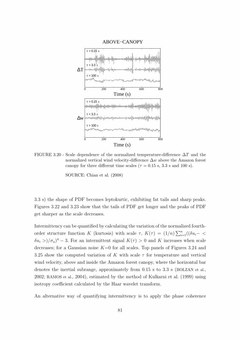
0 200 400 600 800

0 200 400 600 800

T∆

w∆

τ = 100 s

τ = 0.15 s

τ = 3.3 s

τ = 0.15 s

τ = 3.3 s

τ = 100s

Time (s)

Time (s)

ABOVE−CANOPY

FIGURE 3.20 - Scale dependence of the normalized temperature-difference ∆T and thenormalized vertical wind velocity-difference ∆w above the Amazon forestcanopy for three different time scales (τ = 0.15 s, 3.3 s and 100 s).


3.3 s) the shape of PDF becomes leptokurtic, exhibiting fat tails and sharp peaks.

Figures 3.22 and 3.23 show that the tails of PDF get longer and the peaks of PDF

get sharper as the scale decreases.

Intermittency can be quantified by calculating the variation of the normalized fourth-

order structure function K (kurtosis) with scale τ , K(τ) = (1/n)∑n

i=1((δui− <

δui >)/σu)4 − 3. For an intermittent signal K(τ) > 0 and K increases when scale

decreases; for a Gaussian noise K=0 for all scales. Top panels of Figures 3.24 and

3.25 show the computed variation of K with scale τ for temperature and vertical

wind velocity, above and inside the Amazon forest canopy, where the horizontal bar

denotes the inertial subrange, approximately from 0.15 s to 3.3 s (BOLZAN et al.,

2002; RAMOS et al., 2004), estimated by the method of Kulkarni et al. (1999) using

isotropy coefficient calculated by the Haar wavelet transform.

An alternative way of quantifying intermittency is to apply the phase coherence

81

0 200 400 600 800

0 200 400 600 800

T∆

w∆

τ = 0.15

τ = 3.3

s

s

τ = 3.3 s

τ = 0.15 s

τ = 100s

τ = 100s

IN−CANOPY

Time (s)

Time (s)

FIGURE 3.21 - Scale dependence of the normalized temperature-difference ∆T and thenormalized vertical wind velocity-difference ∆w within the Amazon forestcanopy for three different time scales (τ = 0.15 s, 3.3 s and 100 s).


technique using surrogate data by defining a phase coherence index (HADA et al.,

2003; KOGA et al., 2007; KOGA et al., 2008), Cφ(τ) = (SPRS(τ)−SORG(τ))/(SPRS(τ)−SPCS(τ)). This index measures the degree of phase coherence in an original data set

(ORG) by comparing it with two surrogate data sets created from the original data

set: the phase-randomized surrogate (PRS) in which the phases of the Fourier modes

are made completely random, and the phase-correlated surrogate (PCS) in which the

phases of the Fourier modes are made completely equal. The power spectrum of three

data sets ORG, PRS and PCS are kept the same, but their phase distributions are

different. Each length of ORG, PRS and PCS data set is measured by the magnitude

of first-order structure function S1(τ) =∑n

i=1 |ui+τ − ui|. An average of over 100

realizations of the phase shuffling is performed to generate the phase-randomized

surrogate data set SPRS(τ). Cφ(τ)=0 indicates that the phases of the scales τ of the

original data are completely random, whereas Cφ(τ)=1 indicates that the phases are

completely correlated. Bottom panels of Figures 3.24 and 3.25 show the computed

82

-10 -5 0 5 1010

-5

10-4

10-3

10-2

10-1

100

-10 -5 0 5 1010

-5

10-4

10-3

10-2

10-1

100

-10 -5 0 5 1010

-5

10-4

10-3

10-2

10-1

100

-10 -5 0 5 1010

-5

10-4

10-3

10-2

10-1

100

-10 -5 0 5 1010

-5

10-4

10-3

10-2

10-1

100

-10 -5 0 5 1010

-5

10-4

10-3

10-2

10-1

100

ABOVE−CANOPY

PD

FP

DF

PD

F

s

s

sτ = 100

τ = 3.3

τ = 0.15

Vertical Velocity

w

w

w

∆

∆

∆

PD

FP

DF

PD

F

s

s

s

Temperature

τ = 0.15

τ = 3.3

τ = 100

T

T

T

∆

∆

∆

FIGURE 3.22 - Probability density distribution (PDF) of the normalized vertical windvelocity-difference ∆w (left panels) and the normalized temperature-difference ∆T (right panels) fluctuations above the Amazon forest canopyfor three different scales (τ = 0.15 s, 3.3 s and 100.0 s), superposed by aGaussian PDF (gray line).


variation of Cφ with scale τ for temperature and vertical wind velocity above and

inside the Amazon forest canopy.

Figure 3.24 confirms that both kurtosis and phase coherence index can be used to

measure the degree of intermittency and phase coherence in turbulence. Left panels

of Figure 3.24 show that for all scales τ<∼ 35 s the in-canopy vertical velocity is more

intermittent than the above-canopy vertical velocity. Right panels of Figure 3.24

show that for small scales outside the inertial subrange the in-canopy temperature

is more intermittent than the above-canopy temperature; whereas, for scales within

and greater than the inertial subrange the in-canopy temperature is less intermittent

than the above-canopy temperature.

83

-10 -5 0 5 1010

-5

10-4

10-3

10-2

10-1

100

-10 -5 0 5 1010

-5

10-4

10-3

10-2

10-1

100

-10 -5 0 5 1010

-5

10-4

10-3

10-2

10-1

100

-10 -5 0 5 1010

-5

10-4

10-3

10-2

10-1

100

-10 -5 0 5 1010

-5

10-4

10-3

10-2

10-1

100

-10 -5 0 5 1010

-5

10-4

10-3

10-2

10-1

100

IN−CANOPY

PD

FP

DF

PD

F

s

s

s

τ = 0.15

τ = 3.3

τ = 100

∆w

w∆

w∆

PD

FP

DF

PD

F

s

s

s

τ = 0.15

τ = 3.3

τ = 100

T∆

T∆

T∆

Vertical Velocity Temperature

FIGURE 3.23 - Probability density distribution (PDF) of the normalized vertical windvelocity-difference ∆w (left panels) and the normalized temperature-difference ∆T (right panels) fluctuations within the Amazon forest canopyfor three different time scales (τ = 0.15 s, 3.3 s and 100.0 s), superposedby a Gaussian PDF (gray line).


3.2.3 Scalar-velocity dissimilarity in atmospheric intermittent turbu-

lence

The dissimilarity between temperature (scalar) and vertical wind velocity (momen-

tum) can be elucidated by Figures 3.22, 3.23 and 3.24. Figure 3.22 shows that for

scales τ=0.15 s and 3.3 s (a and b in Figure 3.25) the PDFs of temperature fluc-

tuations have longer tails and sharper peaks than the PDFs of vertical velocity

fluctuations, implying that at these scales temperature is more intermittent than

vertical wind velocity above the Amazon forest canopy. The scalar-velocity dissimi-

larity above the canopy is clearly characterized by both kurtosis and phase coherence

techniques in the left panels of Figure 3.25, which show that the above-canopy tem-

perature is more intermittent than vertical wind velocity for all scales τ<∼ 55 s.

In contrast, the right panels of Figure 3.25 show that the scalar-velocity dissimilarity

of the in-canopy turbulence is greatly reduced. The scalar-velocity similarity inside

84

| |

0.01 0.1 1 10 100 10000

0.1

0.2

0.3

0.4

0.5

0.6Above-canopyIn-canopy

| |

0.01 0.1 1 10 100 10000

0.1

0.2

0.3

0.4

0.5

0.6Above-canopyIn-canopy

| |

0.01 0.1 1 10 100 10000

10

20

30

40 Above-canopyIn-canopy

| |

0.01 0.1 1 10 100 10000

10

20

30

40 Above-canopyIn-canopy

TemperatureVertical Velocity

Kur

tosi

s

τ τPh

ase

Coh

eren

ce I

ndex

ττ

Phas

e C

oher

ence

Ind

exK

urto

sis

(sec)

(sec) (sec)

(sec)

FIGURE 3.24 - Kurtosis and phase coherence index of vertical wind velocities (left pan-els) and temperatures (right panels) above and within the Amazon forestcanopy. Thick solid lines denote the in-canopy vertical wind velocity, thindash-dotted lines denote the above-canopy vertical wind velocity, thickdashed lines denote the in-canopy temperature, and thin dotted lines de-note the above-canopy temperature. The bar indicates the inertial sub-range (approximately from τ = 0.15 s to 3.3 s).


the canopy is evidenced in Figure 3.23 which shows that, at τ=0.15 s the PDFs

of temperature and vertical wind velocity have similar sharp peaks and long-tail

statistics.

3.3 Discussion

For numerical simulations and analytic formulation of turbulence based on a set of

deterministic plasma or fluid equations, in the absence of noise, it is natural to ex-

pect that a departure from Gaussianity arises from nonlinear multiscale coupling in

turbulent energy cascade (FRISCH, 1995; DAVIDSON, 2004). In contrast, the observa-

tional data of space plasma turbulence is an admixture of deterministic signal and

stochastic noise. Under this circumstance, a demonstration of finite phase synchro-

nization is required to ascertain the nonlinear origin of non-Gaussian fluctuations.

For magnetic field turbulence in the solar wind, in the absence of strong disturbances

85

| |

0.01 0.1 1 10 100 10000

0.1

0.2

0.3

0.4

0.5

0.6Vertical velocityTemperature

| |

0.01 0.1 1 10 100 10000

0.1

0.2

0.3

0.4

0.5

0.6Vertical velocityTemperature

| |

0.01 0.1 1 10 100 10000

10

20

30

40 Vertical velocityTemperature

| |

0.01 0.1 1 10 100 10000

10

20

30

40 Vertical velocityTemperature

τ

Pha

se C

oher

ence

Inde

x

Pha

se C

oher

ence

Inde

xK

urto

sis

Kur

tosi

s

τ τ (sec)(sec)

τ(sec) (sec)

ABOVE−CANOPY IN−CANOPY

a

bc

a

cb

FIGURE 3.25 - Kurtosis and Phase Coherence Index of vertical wind velocities and tem-peratures above (left panels) and within (right panels) the Amazon forestcanopy. Thick solid lines denote the in-canopy vertical wind velocity, thindash-dotted lines denote the above-canopy vertical wind velocity, thickdashed lines denote the in-canopy temperature, and thin dotted lines de-note the above-canopy temperature. Letters a, b and c indicate scales τ= 0.15 s, 3.3 s and 100.0 s, respectively. The bar indicates the inertialsubrange (approximately from τ = 0.15 s to 3.3 s).


such as ICMEs (subsection 3.1.1) we showed that, within the inertial subrange, the

departure from Gaussianity increases as the scale decreases, which is a characteristic

of intermittent turbulence. Moreover, Figure 3.12 shows that phase synchronization

associated with nonlinear multiscale interactions is the origin of intermittency and

non-Gaussianity, which leads to the formation of large-amplitude phase coherent

(intermittent) structures at small scales. We have identified these large-amplitude

phase coherent structures as spikes in the time series of magnetic-field differences

in Figure 3.24 and fat tails in the PDF and extended flatness in Figure 3.9. Our

computed results are consistent with the Helios analysis by Bruno et al. (2003) of

solar wind intermittency in the inner heliosphere. For slow solar wind at 0.9 AU,

Bruno et al. (2003) obtained the values of 19 for τ = 100 s and 7 for τ = 1000 s for

flatness, which are close to our numerical examples given in Table 3.1.

86

Large-amplitude coherent structures embedded within intermittent magnetic field

turbulence in the foreshock region of Earth’s bow shock have been detected by

Cluster. Eastwood et al. (2003) detected, on 3 February 2002, large-amplitude ultra-

low-frequency (ULF) Alfven waves with wavelength of 3,400 km, in the foreshock

region of Earth’s quasi-parallel bow shock. Stasiewicz et al. (2003) reported the mea-

surement, on 3 February 2002, of the density profiles and wave spectra inside fast

magnetosonic shocklets, 1,000 km in size and amplitude of 10 times the ambient

magnetic field, upstream of a quasi-parallel bow shock. Behlke et al. (2004) ob-

served on 3 February 2002 solitary waves, as bipolar pulses in the spiky electric field

moving at velocities of 400-1,200 km/s along the ambient magnetic field with peak-

to-peak amplitudes of E‖ = 65 mV/m and parallel scale sizes of L‖ ∼ 300− 600 m

∼ 10λD (Debye length), within short large-amplitude magnetic structures (SLAMS)

upstream of a quasi-parallel bow shock. In addition, Parks et al. (2006) detected

ion density holes accompanied by magnetic holes (∼ 3,700 km) upstream of a quasi-

parallel bow shock, which are seen only with upstream particles, suggesting a link

with backstreaming particles interacting with the solar wind. All the aforementioned

observations (found outside of the time interval analyzed in this subsection) refer

to the foreshock region of a quasi-parallel shock which is a patchwork of SLAMS

slowing down and piling up. SLAMS evolve from ULF instabilities excited by coun-

terstreaming plasma populations (SCHWARTZ, 2006) and have amplitudes 2-4 times

larger than the ambient magnetic field, with typical durations of around 10 s and

transverse dimensions of ∼ 1 RE (LUCEK et al., 2004). Although the interval of Clus-

ter data analyzed in this subsection is outside of the foreshock region, we expect that

some of the coherent structures discussed above may contribute to the intermittent

turbulence in this upstream region when IMF connects to bow shock (KELLOGG;

HORBURY, 2005).

Large-amplitude coherent structures in the ambient solar wind have been found by

Helios and ACE. Bruno et al. (2001), Bruno et al. (2003) and Bruno et al. (2005)

reported the observation of coherent structures in the intermittent magnetic field

turbulence between 0.3 to 1 AU using the Helios solar wind data. During a fast solar

wind interval on Julian Day 49-52 1976 when Helios-2 was at 0.9 AU and the solar

wind fluctuations are Alfvenic, they detected one coherent structure related to a flux

tube of scale size ∼ 9 × 105 km (BRUNO et al., 2001). In a recent paper, Borovsky

(2008) studied the statistics of 65,860 flux tubes in the ACE data for the period

1998-2004, and obtained a median scale size of flux tubes of ∼ 6.2× 105 km for slow

87

solar wind and of ∼ 4.2×105 km for fast solar wind. These coherent structures (flux

tubes) are spotted by large changes in the magnetic field direction and the vector

flow velocity, and are associated with large changes in the ion entropy density and

the alpha-to-proton ratio. These flux tubes map to granule and supergranule sizes

on the Sun’s photosphere. Borovsky (2008) suggested a method for using these solar

wind coherent structures for remote sensing of the dynamics of the Sun’s magnetic

carpet. Note that the coherent structures reported by Bruno et al. (2001), Bruno

et al. (2003), Bruno et al. (2005) and Borovsky (2008) have spatial scales ∼ 105

km which correspond to time scales ∼ 103 s (assuming Taylor’s hypothesis and

Vsw ∼ 4 × 102 km/s). These large-scale flux tubes might be coherent structures

convected by the solar wind from the base of the solar atmosphere (BRUNO et al.,

2001; BOROVSKY, 2008).

It is worth mentioning that the most intermittent events in the solar wind turbu-

lence, which occur at time scales of the order of a few minutes, have been identi-

fied as current sheets and shock waves (VELTRI; MANGENEY, 1999; VELTRI, 1999;

ALEXANDROVA et al., 2008). These small-scale intermittent structures may be related

to locally occurring magnetic reconnections (CHANG et al., 2004; ZHOU et al., 2004;

GRECO et al., 2009) and may play an important role in the phase synchronization

observed by Figure 3.12 in the interplanetary magnetic field turbulence.

In section 3.1.2 we studied and compared non-Gaussianity and phase synchroniza-

tion in solar-terrestrial magnetic field turbulence in two scenarios: a non-ICME event

and an ICME event. For each scenario, we calculated first kurtosis and the phase

coherence index for an active region and a quiet region, respectively, in the solar

photosphere. We then applied the same techniques to solar wind turbulence using

in situ data. The response of the Earth’s geomagnetic field using data from ground

magnetometers in Brazil was presented. In particular, we showed that the interplan-

etary magnetic field turbulence downstream of the ICME shock is closely correlated

with the geomagnetic turbulence detected on the ground.

In section 3.2 we analyzed day-time atmospheric data above and within an Amazon

forest canopy. We showed that the scale dependence of kurtosis and phase coherence

index for vertical wind velocity and temperature above and within canopy exhibit

similar behaviors, as seen in Fig. 3.24. In particular, both techniques demonstrate

a clear enhancement of scalar-velocity similarity for in-canopy turbulence in com-

parison to its above-canopy counterpart, as seen in Figure 3.25. Our results prove

88

that the atmospheric intermittent turbulence, above and within the Amazon forest

canopy, is generated by the phase coherence due to nonlinear wave-wave interactions.

Turbulence consists of an admixture of chaos and noise. Recent studies have identi-

fied the chaotic nature of the solar-terrestrial environment (MACEK, 1998; CHIAN et

al., 2006) and the atmospheric turbulence above the Amazon forest (CAMPANHARO

et al., 2008), which have been confirmed by computer simulations of temporal chaos

and spatiotemporal chaos in fluids and plasmas (CHIAN et al., 2006; REMPEL; CHIAN,

2007; REMPEL et al., 2007). It is likely that phase coherence and chaotic synchro-

nization are the origin of energy bursts and coherent structures of turbulence in the

complex earth-ocean-space system (HE; CHIAN, 2003; HE; CHIAN, 2005).

The results of this chapter indicate that variations of kurtosis and the phase co-

herence index are similar across scales. Since kurtosis can be interpreted as the

energy squared (see subsection 2.1.3), it can also be regarded as a measurement

of non-Gaussianity (i.e., synchronization) using the amplitude information. Hence,

our observational results show that there is a duality between phase synchronization

(quantified by the phase coherence index) and amplitude synchronization (quantified

by kurtosis).

89

4 THEORY OF SYNCHRONIZATION IN SPATIOTEMPORAL IN-

TERMITTENCY

In this Chapter the mathematical tools described in Section 2.2 are applied to the

Benjamin-Bona-Mahony (BBM) equation, a nonlinear model of drift waves in mag-

netized plasmas and shallow water waves in fluids. This model is also called the

regularized long-wave equation (RLWE). In Section 4.1 we present the equation and

demonstrate that the coupling of chaotic saddles is responsible for the on-off inter-

mittency at the onset of spatiotemporal chaos. Section 4.2 is devoted to measure the

degree of amplitude-phase synchronization in the BBM equation. We perform an

analysis of the amplitude and phase synchronization due to multiscale interactions

in the temporally and spatiotemporally chaotic attractor embedded in the chaotic

attractor at the onset of spatiotemporal chaos.

4.1 Spatiotemporal intermittency and chaotic saddles in the Benjamin-

Bona-Mahony (BBM) equation

4.1.1 The Benjamin-Bona-Mahony equation

The unidirectional propagation of long waves in fluids with small but finite amplitude

in systems with nonlinearity and dispersion can be described by the Korteweg-de

Vries (KdV) equation, which in dimensionless form is given by (BENJAMIN et al.,

1972; DODD et al., 1982; NICHOLSON, 1983)

∂tu+ ∂xu+ u∂xu+ ∂xxxu = 0. (4.1)

Equation (4.1) is often written without the second term, after taking x′ = x − t

and t as independent variables. The KdV equation was originally derived for water

waves and has been used as a model for long waves in many other physical systems

(DODD et al., 1982), e.g., nonlinear ion-acoustic waves in plasmas (NICHOLSON, 1983).

However, some mathematical properties of the KdV equation such as existence and

stability of solutions are difficult to study (BENJAMIN et al., 1972). Furthermore,

there are other problems, mainly due to the dispersion term. For example, from the

linear dispersion relation of Eq. (4.1)

ω = k − k3, (4.2)

91

one can observe that the phase velocity Vph = ω/k becomes negative for k2 > 1,

which is inconsistent with the assumption of forward-travelling waves, used in the

derivation of Eq. (4.1) (BENJAMIN et al., 1972). Moreover, the group velocity

dω

dk= 1− 3k2, (4.3)

does not have any lower limit, thus there is no bound to the velocity with which

short wavelength features propagate. These impediments have led to the pursuit of

an alternative model. The regularized long-wave equation was proposed by Peregrine

(1966) and Benjamin et al. (1972) as an alternative to the KdV equation. It was

later derived by He and Salat (1989) as a model for nonlinear drift waves in plasmas,

with a periodic driving term and a linear damping term introduced ad hoc in order

to study transition to chaos. The driven-damped regularized long wave equation is

given by (HE; SALAT, 1989; REMPEL; CHIAN, 2007; HE, 1998; HE; CHIAN, 2004; HE;

CHIAN, 2003; HE; CHIAN, 2005)

∂tu+ c∂xu+ fu∂xu+ a∂txxu = −νu− ε sin(κx− Ωt), (4.4)

where a, c, and f are constants, ν is a damping parameter, ε is the driver amplitude,

κ is the driver wavenumber and Ω is the driver frequency. Originally, Peregrine

(1966) obtained Eq. (4.4) (without the two terms on the right hand side) from

the momentum equation for the mean horizontal velocity of water u(x, t) of an

irrotational flow by assuming that waves only travel in one direction and the ratios

between wave amplitude and water depth and between water depth and wavelength

are small, where wavelength means the distance in which significant changes in

surface height occur. The third-order derivative term in Eq. (4.4) expresses the effect

of the vertical acceleration of water on pressure. In the absence of forcing (ε = 0),

the linear dispersion relation is

ω(k) = (iν − ck)/(ak2 − 1), (4.5)

from which the phase velocity can be obtained

92

Vph = − c

ak2 − 1+

iν

k(ak2 − 1). (4.6)

Assuming a < 0 and c > 0, Re[Vph] > 0 for all k. The group velocity

Vg = − c

ak2 − 1+ 2ack2

(1

ak2 − 1

)2

− 2iaνk

(1

ak2 − 1

)2

(4.7)

approaches zero for large k, which means that high wavenumber features do not

propagate. Existence, uniqueness and stability of solutions of the RLWE have been

formally demonstrated by Benjamin et al. (1972).

We define periodic boundary conditions u(x, t) = u(x + 2π, t), and fix a = −0.287,

c = 1, f = −6, ν = 0.1, κ = 1 and Ω = 0.65. These parameter values can be chosen

arbitrarily, with the exception of a, which must be negative for physical reasons

and to avoid numerical instability (HE; SALAT, 1989). Here, the values are chosen

in order to study the transition to spatiotemporal chaos previously identified by He

(1998). Thus, the driver amplitude ε is the only control parameter. From Eq. (4.5),

since a < 0 and ν > 0, Im[ω(k)] < 0 for all k. Thus, all modes are linearly damped.

This is in contrast to the Kuramoto-Sivashinsky equation studied by Rempel et al.

(2007), where there was a band of linearly unstable Fourier modes. In the case of the

RLWE, the external driver is necessary to destabilize the mode with wave number

k = 1, as discussed below.

We solve equation (4.4) with the spectral (Galerkin) method, by expanding u(x, t)

in a Fourier series following Rempel and Chian (2007)

u(x, t) =N∑

k=−N

uk(t)eikx, (4.8)

where k = 2πn/L, n = −N, ..., N , L = 2π is the system length, and i =√−1. We

set N = 32. By introducing (4.8) into (4.4) one obtains a set of ordinary differential

equations in terms of the complex Fourier coefficients uk(t)

93

(1− ak2)dukdt

= −ickuk − νuk +ε

2sin(Ωt)δ1,k +

iε

2cos(Ωt)δ1,k − [ifkukuk]k, (4.9)

where δ is the Kronecker delta and the last term on the right-hand side is the

Fourier transform of fu∂xu, which is responsible for nonlinear wave coupling. In

order to compute this term, the pseudospectral method is used, where the derivative

is obtained in the Fourier space, ∂xu → ikuk. Next, both ikuk and uk are inverse-

Fourier transformed to real space, where the multiplication fu∂xu is performed.

Finally, the result is Fourier transformed again and inserted into equation (4.9).

Numerical integration is performed using the lsodar integrator (PETZOLD, 1983), a

variable-step integrator available in www.netlib.org. At each time step, 1/3 of the

high k modes are set to zero in order to avoid aliasing errors (TAJIMA, 1989). Thus,

the effective number of modes is N = 20. From equation (4.9), it can be seen that

in the presence of an external driver (ε 6= 0) energy is injected into the mode k = 1

and spreads towards other modes through the nonlinear term. Thus, the forcing and

nonlinear terms are responsible for driving the system away from equilibrium and

leading the system to chaos.

4.1.2 Transition to spatiotemporal chaos

The transition to spatiotemporal chaos (STC) can be easily recognized as a sudden

change in the spatiotemporal patterns of the numerical solutions of equation (4.4).

Figure 4.1 shows the asymptotic solutions obtained for two values of the control

parameter ε. The first regime (Fig. 4.1, upper panel), obtained for ε = 0.199, is

regular in space, but a positive value of the maximum Lyapunov exponent (λ1 ≈0.05) for the attractor indicates that the dynamics is temporally chaotic (TC). The

Lyapunov exponents are obtained from the eigenvalues of the linearized vector field

along a trajectory, and are computed with the code given in Wolf et al. (1985),

where a Gram-Schmidt orthonormalization process which employs the Euclidean

norm is used and base 2 logarithm is adopted for the exponents. The lower panel

of Fig. 4.1 shows that in the second regime (ε = 0.201) the spatiotemporal patterns

are disordered in both space and time. The maximum Lyapunov exponent for the

attractor STCA has jumped to λ1 ≈ 0.12. The transition from spatial regularity

to spatial irregularity is due to an attractor-widening crisis that occurs after the

collision of the spatially regular attractor with an unstable saddle orbit, and has

94

(x, t)u

020

60

020

4060

80

−10

10

0

40

tx/

(x, t)u

020

60

020

4060

80

−10

10

0

40

tx/

x∆

x∆

(ε = 0.199)TCA

(ε = 0.201)STCA

FIGURE 4.1 - Spatiotemporal patterns u(x, t) of the regularized long wave equation, forε = 0.199 (temporally chaotic attractor, TCA, upper panel), and ε = 0.201(spatiotemporally chaotic attractor, STCA, lower panel).

SOURCE: Rempel et al. (2009)

95

uu

FIGURE 4.2 - Time-averaged power spectra in the k wavenumber domain, for ε = 0.199(TCA regime, dashed line) and ε = 0.201 (STCA regime, solid line), forsimulations with N = 32 (left) and N = 512 (right) Fourier modes.


been described in a series of papers (HE, 1998; HE; CHIAN, 2004; HE; CHIAN, 2003).

The energy distribution among Fourier modes can be seen in the time-averaged

power spectra 〈|uk|2〉 depicted in Fig. 4.2 for N = 32 (left) and for N = 512 (right).

The spectrum in the temporally chaotic attractor (TCA) regime (ε = 0.199, dashed

line) is narrower than in the spatiotemporally chaotic attractor (STCA) regime (ε =

0.201, solid line). This indicates that at the onset of STC, when the spatial regularity

is destroyed, spectral energy cascades to neighboring modes due to nonlinear wave-

wave interactions, increasing the number of active modes. The energy spreading

remains essentially the same for N = 32 and N = 512.

The amount of spatial disorder can be quantified by means of the Fourier power

spectral entropy (REMPEL et al., 2007; POWELL; PERCIVAL, 1979; XI; GUNTON, 1995),

introduced in Subsection 2.2.2

SAk (t) = −N∑k=1

pk(t) ln(pk(t)), (4.10)

where pk(t) is the relative weight of a Fourier mode k at an instant t

pk(t) =|uk(t)|2∑Nk=1 |uk(t)|

2. (4.11)

96

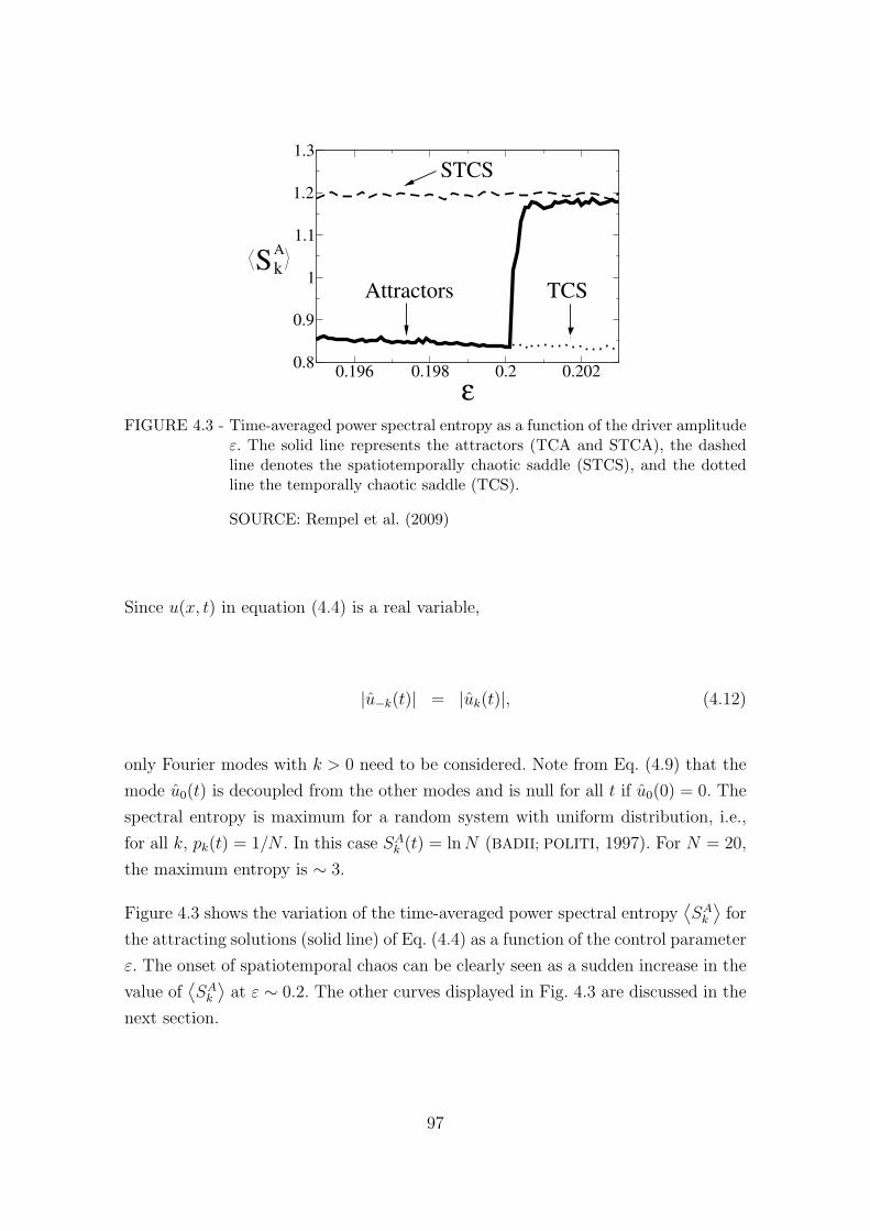
0.196 0.198 0.2 0.2020.8

0.9

1

1.1

1.2

1.3

ε

TCS

STCS

Attractors

SA

k

FIGURE 4.3 - Time-averaged power spectral entropy as a function of the driver amplitudeε. The solid line represents the attractors (TCA and STCA), the dashedline denotes the spatiotemporally chaotic saddle (STCS), and the dottedline the temporally chaotic saddle (TCS).


Since u(x, t) in equation (4.4) is a real variable,

|u−k(t)| = |uk(t)|, (4.12)

only Fourier modes with k > 0 need to be considered. Note from Eq. (4.9) that the

mode u0(t) is decoupled from the other modes and is null for all t if u0(0) = 0. The

spectral entropy is maximum for a random system with uniform distribution, i.e.,

for all k, pk(t) = 1/N . In this case SAk (t) = lnN (BADII; POLITI, 1997). For N = 20,

the maximum entropy is ∼ 3.

Figure 4.3 shows the variation of the time-averaged power spectral entropy⟨SAk⟩

for

the attracting solutions (solid line) of Eq. (4.4) as a function of the control parameter

ε. The onset of spatiotemporal chaos can be clearly seen as a sudden increase in the

value of⟨SAk⟩

at ε ∼ 0.2. The other curves displayed in Fig. 4.3 are discussed in the

next section.

97

4.1.3 Transient and intermittent spatiotemporal dynamics

By neglecting the dissipation and forcing terms on the right-hand side of Eq. (4.4),

after multiplication by u and integration in the spatial domain, one can obtain an

equation to describe the temporal evolution of the“wave energy”, which is a constant

of motion for ν = ε = 0 (HE; SALAT, 1989; HE; CHIAN, 2005; BENJAMIN, 1972)

E(t) =1

4π

∫ 2π

0

[u2 − au2

x

]dx . (4.13)

The details of the derivation of this quantity can be found in Appendix D (Chapter

10) We use the time series of the wave energy to identify transient and intermittent

behaviors in the RLWE. Another quantity that has proven useful in this task is

the time series for the height of the main peak of the power spectrum h (REMPEL

et al., 2007). Figure 4.4 shows the time series for the wave energy E and the main

peak height h. In the TC regime (Fig. 4.4, left panels) the time series of E and h

display an initial behavior of high-level fluctuations before converging asymptotically

to a “laminar” state with lower variability, corresponding to the TCA of Fig. 4.1

(upper panel). In the STC regime (Fig. 4.4, right panels) the time series of E and

h display intermittent switchings between “bursty” (high variability) and “laminar”

(low variability) behaviors. It is important to distinguish the nature of this TC-STC

intermittency found in the RLWE from the spatiotemporal intermittency reported

by Chate and Manneville (1987), where patches of laminar and bursty behaviors

coexist in space. Here the bursty phases are clearly localized in time, but extend over

the whole space, similar to the spatiotemporal intermittency found in the damped

Kuramoto-Sivashinsky equation with periodic boundary conditions (REMPEL et al.,

2007) and experiments with liquid columns hanging below an overflowing circular

dish (BRUNET; LIMAT, 2004).

As mentioned before, chaotic transients are due to the presence of chaotic saddles in

the phase space. We adopt a Poincare map in which a point is plotted every time the

flow of Eqs. (4.9) crosses the plane Re(u1(t)) = 0 with d[Re(u1(t))]/dt > 0. Then,

we employ the sprinkler method (KANTZ; GRASSBERGER, 1985; HSU et al., 1988) to

find chaotic saddles. In Figure 4.5 the attracting and non-attracting chaotic sets are

represented as projections of the Poincare points on the [Re(u4),Re(u5)] plane. At

ε = 0.199, prior to the onset of STC, it is possible to find a chaotic saddle coexisting

with the temporally chaotic attractor (TCA). This chaotic saddle is responsible for

98

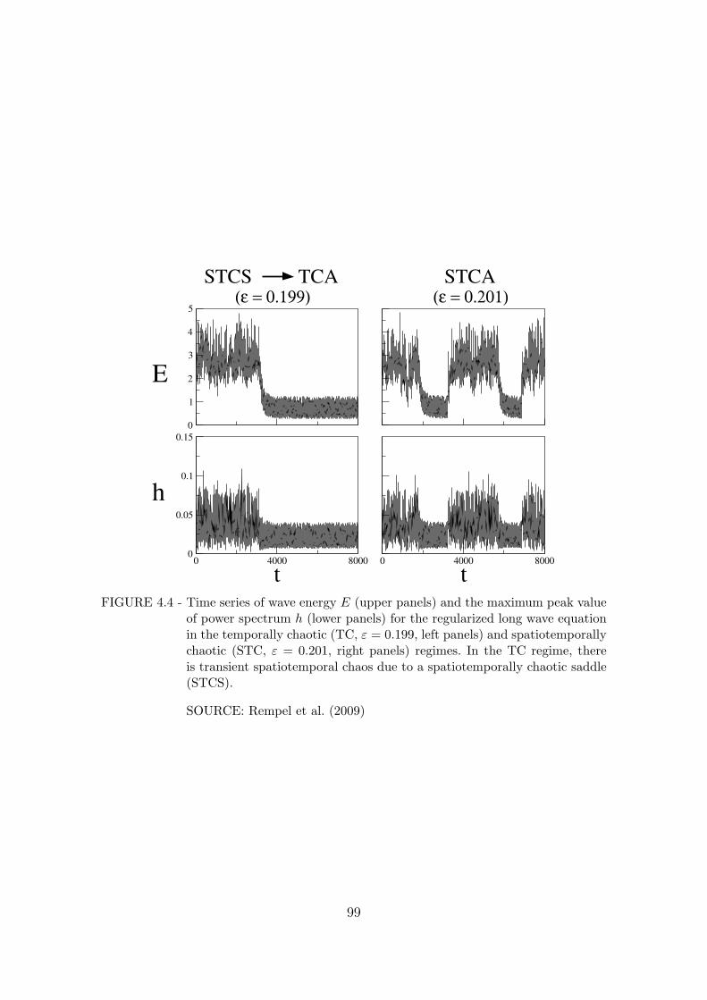
0

1

2

3

4

5

0 4000 80000

0.05

0.1

0.15

0 4000 8000

h

E

t t

STCATCASTCS

(ε = 0.199) (ε = 0.201)

FIGURE 4.4 - Time series of wave energy E (upper panels) and the maximum peak valueof power spectrum h (lower panels) for the regularized long wave equationin the temporally chaotic (TC, ε = 0.199, left panels) and spatiotemporallychaotic (STC, ε = 0.201, right panels) regimes. In the TC regime, thereis transient spatiotemporal chaos due to a spatiotemporally chaotic saddle(STCS).


99

transient spatiotemporal chaos, and is duly named spatiotemporally chaotic saddle

(STCS) (REMPEL; CHIAN, 2007; REMPEL et al., 2007). Figure 4.5 (upper panel) de-

picts the TCA (black) and the STCS (gray) for ε = 0.199. The latter surrounds

the region occupied by the TCA. After the transition to STC (ε = 0.201, Fig. 4.5

(middle panel)), the attractor expands abruptly to include the region previously oc-

cupied by the STCS. If one applies the sprinkler method in this regime, two chaotic

saddles embedded in the spatiotemporally chaotic attractor (STCA) can be found.

They are shown in Fig. 4.5, where the STCA (middle panel) is decomposed into a

spatiotemporally chaotic saddle (gray) and a temporally chaotic saddle (TCS, black)

(lower panel) which evolves from the destabilized TCA. In the sprinkler method, the

chaotic saddle is approximated by points from trajectories that follow long transients

before escaping from a predefined restraining region of the phase space. Given the

difficulty in defining a restraining region in a high-dimensional phase-space, we use

the different levels of wave energy displayed by the TC and STC regimes to identify

the “restraining regions”. To find the STC saddle, a large set of initial conditions is

iterated and those trajectories for which E(t) > 1.2 for 100 consecutive iterations of

the Poincare map (t ≈ 1000) are considered to be in the vicinity of the STC saddle.

For each of those trajectories, the first 40 and last 40 iterations are discarded and

only 20 points are plotted. For the TC saddle, the restraining region is defined as

above, but with E(t) < 1.2, instead. This threshold of E(t) is found after an in-

spection of the variability of E(t) in Fig. 4.4. The number of iterations discarded is

chosen after some trial-and-error (HSU et al., 1988).

The attractor decomposition mentioned in the previous paragraph suggests that

chaotic saddles dominate the spatiotemporal intermittent dynamics found after the

onset of STC. Their signatures can be seen in the time series shown in Fig. 4.4. The

STCS governs the dynamics of the initial transient in the left panel (TC regime),

and the bursty periods in the right panel (STC regime). Moreover, the similarity

between the TCA regime before the STC transition and the laminar phases after

the STC transition are due to the fact that, after the onset of STC, the temporally

chaotic attractor (TCA) loses its stability, becoming a temporally chaotic saddle

(TCS), which governs the laminar periods in the STCA regime. The TC-STC in-

termittency consists of random switchings between phases where the dynamics is

basically governed by TCS and STCS, respectively.

As the control parameter ε is increased beyond the transition point, the average

100

5u

Re(

)5

Re(

)u

5R

e(

)

u

TCA

ε = 0.201

TCS

STCA ε = 0.201

ε = 0.199STCS

STCS

4uRe( )

FIGURE 4.5 - Projections of attracting and non-attracting chaotic sets for the regularizedlong wave equation, for ε = 0.199 (upper panel), showing the temporallychaotic attractor (TCA, black) and the spatiotemporally chaotic saddle(STCS, gray); for ε = 0.201 (middle panel), showing the spatiotemporallychaotic attractor (STCA), which is decomposed in the lower panel intoa temporally chaotic saddle (TCS, black) and a spatiotemporally chaoticsaddle (STCS, gray).


101

log

10(τ

)

-4 -3.5 -3 -2.50

0.5

1

1.5

2

2.5

γ ∼ −1.05

10log ( )ε − ε

c

FIGURE 4.6 - Average duration of laminar intervals τ as a function of the departure fromthe critical value of the control parameter (εc = 0.2), in log-log scale, forthe regularized long-wave equation. The straight line shows a least-squaresfit with slope γ ∼ −1.05.


duration of the laminar periods τ decreases as a power law. In Fig. 4.6 we plot τ

as a function of the departure from the critical value of the control parameter (here

taken as εc = 0.2), in log-log scale. This result indicates that the STCS dominates

the spatiotemporal dynamics of the STCA when the value of the control parameter ε

is increased. This can also be seen in Fig. 4.3, where the values of the time-averaged

spectral entropy for STCS and TCS are represented by the dashed and dotted lines,

respectively. The power spectral entropy of STCA rapidly approaches the entropy of

STCS after the transition at εc ∼ 0.2. It is clear that the power spectral entropy of

STCS for ε < εc can be used to predict the dynamics in STCA for ε > εc as pointed

out in Rempel and Chian (2007).

4.2 Synchronization in the BBM equation

In this Section we investigate the amplitude and phase synchronization related with

multicale interactions after the onset of spatiotemporal chaos (on-off intermittency)

using the power-phase spectral entropies and the power-phase disorder parameters

introduced in Section 2.2. After the onset of spatiotemporal chaos (ε ∼ 0.2), a trajec-

tory on the spatiotemporally chaotic attractor that initially spends some time in the

102

vicinity of the spatiotemporally chaotic saddle (off-state in Figure 4.7) will escape

from it and approach the vicinity of the temporally chaotic saddle (on-state in Fig.

4.7). This process repeats itself back-and-forth, leading to an on-off spatiotemporal

intermittency seen in the time series of the “wave energy”E for ε = 0.20005 (upper

left-hand side panel of Fig. 4.7; see also left-hand side panels of Fig. 4.4). The middle

left-hand side panel show the Fourier power spectral entropy SAk and the bottom left-

hand side panel show the amplitude disorder parameter DAk . The upper right-hand

side panel shows the same time series of E, the middle right-hand side panel shows

the Fourier phase spectral entropy Sφk and the bottom right-hand side panel shows

the phase disorder parameter Dφk . The red lines denote the average taken within a

time window of 1256 time units to facilitate the visualization of the on-off states.

This Figure shows that the amplitude and phase dynamics are more synchronized

during the “on” stages (i.e. there is a lower degree of entropy and disorder) while

the “off” stages are characterized by a lower degree of synchronization (i.e. higher

degree of entropy and disorder). In particular, Sφk (t) shows that the transition from

the laminar (on) state to the bursty (off) state is much faster than the transition

from the bursty state to the laminar state.

In Section 4.1 it was demonstrated that the transient regimes in the time series of on-

off spatiotemporal intermittency at the onset of spatiotemporal chaos are related to

the chaotic saddles embedded in a chaotic attractor (REMPEL; CHIAN, 2007; REMPEL

et al., 2007; REMPEL et al., 2009). Fig 4.8 shows a three-dimensional projection of the

39-dimensional Poincare hyper-surface of section of chaotic attractors and chaotic

saddles found before and after transition. Figure 4.8(a) shows the STCS detected

by using the sprinkler method for ε = 0.199, before the onset of spatiotemporal

chaos. This chaotic saddle governs the dynamics of transients before converging to

the temporally chaotic attractor (TCA) which is shown in Fig. 4.8(b). Note that

the TCA occupies a smaller volume of phase space, which resembles a surface. In

contrast, the STCS occupies a larger, sphere-like volume of phase space. At ε ∼ 0.2,

a crisis occurs due to a chaotic attractor-chaotic saddle collision involving the TCA

and the STCS. At crisis, the TCA loses its stability and is converted to a temporally

chaotic saddle (TCS), as seen in Fig. 4.8(c) for ε = 0.20005; the STCS is robust and

persists after crisis, also shown in Fig. 4.8(c). At the onset of spatiotemporal chaos,

the TCS becomes coupled to the STCS through the coupling unstable periodic or-

bits to form a STCA, as seen in Fig. 4.8(d), which occupies almost the same region

of phase space as the pre-crisis STCS and TCA. The TCS and the STCS constitute

103

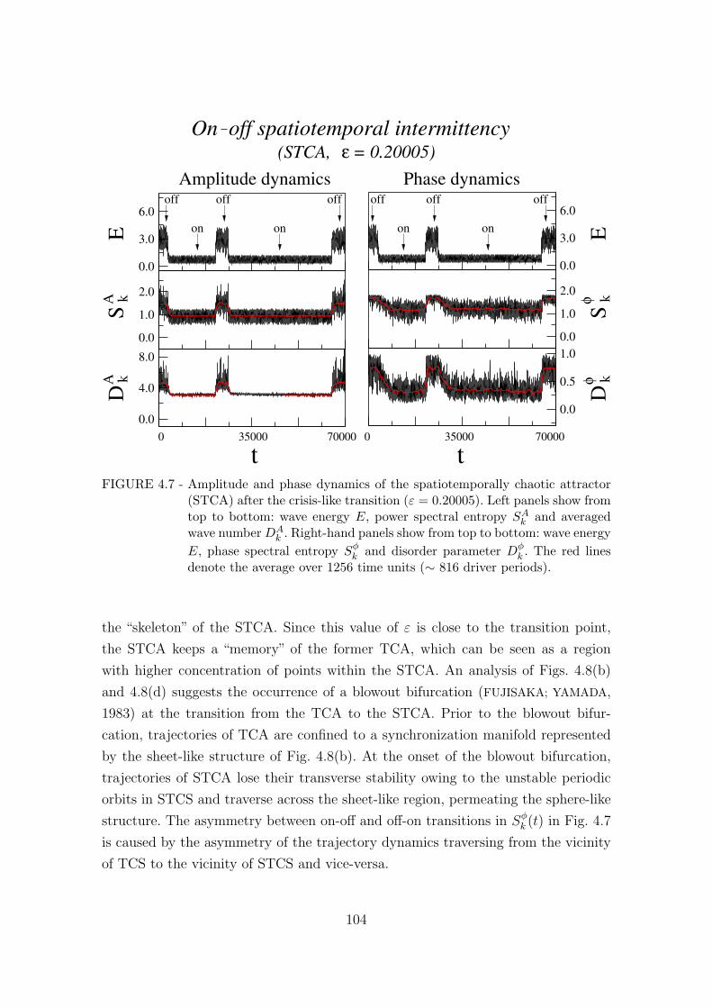
On off spatiotemporal intermittency

0.0

3.0

6.0

0.0

1.0

2.0

0.0

0.5

1.0

0.0

3.0

6.0

0.0

4.0

8.0

0.0

1.0

2.0

AD

k

Dφ k

= 0.20005)ε(STCA,

Skφ

SA k

E

Phase dynamicsoffoff

on

offoff

on

off

on on

off

Amplitude dynamics

E

0 70000

t0 7000035000

t35000

FIGURE 4.7 - Amplitude and phase dynamics of the spatiotemporally chaotic attractor(STCA) after the crisis-like transition (ε = 0.20005). Left panels show fromtop to bottom: wave energy E, power spectral entropy SAk and averagedwave number DA

k . Right-hand panels show from top to bottom: wave energyE, phase spectral entropy Sφk and disorder parameter Dφ

k . The red linesdenote the average over 1256 time units (∼ 816 driver periods).

the “skeleton” of the STCA. Since this value of ε is close to the transition point,

the STCA keeps a “memory” of the former TCA, which can be seen as a region

with higher concentration of points within the STCA. An analysis of Figs. 4.8(b)

and 4.8(d) suggests the occurrence of a blowout bifurcation (FUJISAKA; YAMADA,

1983) at the transition from the TCA to the STCA. Prior to the blowout bifur-

cation, trajectories of TCA are confined to a synchronization manifold represented

by the sheet-like structure of Fig. 4.8(b). At the onset of the blowout bifurcation,

trajectories of STCA lose their transverse stability owing to the unstable periodic

orbits in STCS and traverse across the sheet-like region, permeating the sphere-like

structure. The asymmetry between on-off and off-on transitions in Sφk (t) in Fig. 4.7

is caused by the asymmetry of the trajectory dynamics traversing from the vicinity

of TCS to the vicinity of STCS and vice-versa.

104

3R

eu

3R

eu

3R

eu

3

Re

u

(ε = 0.199)(ε = 0.199)TCA(a) (b)STCS

Poincare plots of chaotic saddles & chaotic attractors´

(ε = 0.20005)STCS + TCS(c) STCA(d)

0.1

0.2 0.1

0.1 0.2

0.1

0.1

0.2 0.1

2Reu 2

Imu

0.1

0.0

0.1

0.1

0.2 0.1

2Reu

2

Imu

0.1

2Reu

2

Imu

2Reu

2

Imu

0.1

0.0

0.1

0.10.0

0.10.0

0.0

0.1

0.1

0.10.0

0.1

0.10.0

0.00.1

0.0

0.10.0

0.10.0

0.0

0.1

(ε = 0.20005)

FIGURE 4.8 - (a) Three-dimensional projection of the Poincare hyper-surface of section ofthe spatiotemporal chaotic saddle (STCS) previous to the crisis-like tran-sition. (b) The temporally chaotic atrractor (TCA) previous to the tran-sition. (c) The temporally chaotic saddle (TCS, blue) and STCS (yellow)after transition. (d) The spatiotemporally chaotic attractor (STCA) aftertransition.

105

0.0

2.0

4.0

0.0

1.0

2.0

0.0

4.0

8.0

0.0

1.0

2.0

0.0

0.5

1.0

ADk

Dφ k

SA k

Skφ

E

0 12000 024000 12000 24000

t t

ε( = 0.20005)

Amplitude phase dynamics of chaotic saddles

TCS STCS

FIGURE 4.9 - Amplitude and phase dynamics of the temporally chaotic saddle (TCS, leftpanels) and the spatiotemporally chaotic saddle (STCS, right panels) afterthe crisis-like transition (ε = 0.20005). From top to bottom: wave energyE, spectral entropy SAk , averaged wave number DA

k , phase entropy Sφk anddisorder parameter Dφ

k . The red lines denote the average over 1256 timeunits (∼ 816 driver periods).

106

The degree of amplitude-phase synchronization in the chaotic saddles (TCS and

STCS) embedded in the STCA at the onset of spatiotemporal chaos can be deter-

mined by calculating the Fourier power and phase entropies and the amplitude-phase

disorder parameters. We used the stagger-and-step procedure (SWEET et al., 2001)

for the computation of long trajectories which approximate chaotic saddles in a

high-dimensional phase space. This method allows us to obtain an arbitrarily long

pseudo-trajectory of a chaotic saddle. Figure 4.9 shows the amplitude and phase

dynamics of the chaotic saddles found in ε = 0.20005. The left-hand side panels

show, from top to bottom, the time series of “wave energy” E , the Fourier power

spectral entropy SAk , the amplitude disorder parameter DAk , the Fourier phase spec-

tral entropy Sφk and the phase disorder parameter Dφk of TCS. The right-hand side

panels show, from top to bottom, the time series of “wave energy” E, the Fourier

power spectral entropy SAk , the amplitude disorder parameter DAk , the Fourier phase

spectral entropy Sφk and the phase disorder parameter Dφk of STCS. The red line

denotes the averaging over 1256 time units. A comparison of Figs. 4.7 and 4.9 show

that the average values of SAk ∼ 0.93, DAk ∼ 3.1, Sφk ∼ 1.01 and Dφ

k ∼ 0.31 of the

TCS in Fig. 4.9 are close to the corresponding values of the on-state of Fig. 4.7;

moreover, the average values of SAk ∼ 1.48, DAk ∼ 4.65, Sφk ∼ 1.67 and Dφ

k ∼ 0.75

of the STCS in Fig. 4.9 are close to the corresponding values of the off-state of Fig.

4.7. This confirms that the on-off states of the spatiotemporal intermittency at the

onset of permanent chaos correspond to the system trajectory traversing the vicinity

of TCS and STCS, respectively.

The energy distribution among Fourier modes in the k wavenumber domain can be

examined by constructing the time-averaged power spectrum⟨|uk|2

⟩. In addition,

we computed the time-averaged phase-difference spectrum 〈|δφk|〉 as a qualitative

measurement of synchronization among Fourier modes. Smaller values of 〈|δφk|〉 cor-

respond to a higher degree of synchronization between Fourier modes k and k + 1.

Fig. 4.10 shows both Fourier power and phase-difference spectra for ε = 0.21, corre-

sponding to the STC regime, for the STCA (red), STCS (yellow) and TCS (blue).

The power spectrum of both STCA and STCS are broader than the TCS, indicating

that the energy is spread among Fourier modes, while the TCS has its energy con-

centrated in a narrow band of wavenumbers. The phase-difference spectra of STCA

and STCS display a tendency to increase with k, suggesting that synchronization

is lower at high wavenumbers. The phase-difference spectra of TCS is, in general,

lower than the STCA and STCS, which is consistent with the fact that the TCS

107

5 10 15 20

10-3

10-2

10-1

STCASTCSTCS

5 10 150

1×10-3

2×10-3

3×10-3

4×10-3

5×10-3

k

2|u | δφ | |

k

Power spectrum Phase spectrum

k k

FIGURE 4.10 - Left panel: time-averaged power spectra⟨|uk|2

⟩for ε = 0.21, of the spa-

tiotemporally chaotic attractor (STCA, red thin line), the spatiotempo-rally chaotic saddle (STCS, yellow thick line) and the temporally chaoticsaddle (TCS, blue thick line). Right panel: time-averaged phase-differencespectra 〈|δφk|〉 of STCA, STCS and TCS.

represents synchronized (“on”) states.

Next, we compute the Lyapunov spectrum of chaotic sets (YAMADA; OKHITANI,

1988; YAMADA; OHKITANI, 1998) before and after the onset of spatiotemporal chaos.

We use the method of Gram-Schmidt orthogonalization (SHIMADA; NAGASHIMA,

1979) and order the Lyapunov exponents as λj > λj+1. The spectrum of rescaled

Lyapunov exponents λj/H of chaotic attractors and chaotic saddles before and after

transition are shown in the top panel of Fig. 4.11, where H denotes the Kolmogorov-

Sinai entropy (Equation (2.43)). Before transition (ε = 0.199), the TCA (green)

has only one positive Lyapunov exponent (λ1 ∼ 0.052418), whereas the pre-crisis

STCS (orange) has 14 positive Lyapunov exponents. After transition (ε = 0.21), the

Lyapunov spectra of both the STCA (red) and the post-crisis STCS (yellow) display

14 positive Lyapunov exponents, whereas the TCS (blue) only has one positive

exponent (λ1 ∼ 0.061873). The similarity between λ1 of TCA before transition and

TCS after transition is due to the fact that, after the onset of STC (ε ∼ 0.2), the

TCA loses its stability becoming a TCS. At ε = 0.21, the Lyapunov spectrum of

STCA has numerical values almost identical to the spectrum of STCS, except for

j ≥ 12. The difference between the Lyapunov spectra of STCA and STCS for j ≥ 12

can be attributed to the fact that both TCS and STCS contribute to the dynamics

of STCA, hence the Lyapunov spectra of STCA is a nonlinear combination of both

TCS and STCS.

108

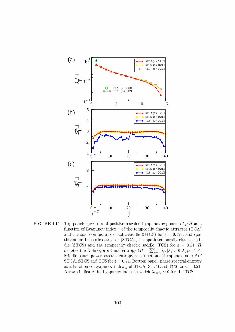
0 5 10 1510-4

10-2

100

λ j/H

TCA (ε = 0.199)STCS (ε = 0.199)

(a)

(b)

STCA (ε = 0.21)STCS (ε = 0.21)TCS (ε = 0.21)

0 10 20 30 401

2

3

4

5

⟨Sj⟩

j0 = 2

Aφ

STCA (ε = 0.21)STCS (ε = 0.21)TCS (ε = 0.21)

0 10 20 30 40j

1

2

3

⟨Sj⟩

STCA (ε = 0.21)STCS (ε = 0.21)TCS (ε = 0.21)

(c)

FIGURE 4.11 - Top panel: spectrum of positive rescaled Lyapunov exponents λj/H as afunction of Lyapunov index j of the temporally chaotic attractor (TCA)and the spatiotemporally chaotic saddle (STCS) for ε = 0.199, and spa-tiotemporal chaotic attractor (STCA), the spatiotemporally chaotic sad-dle (STCS) and the temporally chaotic saddle (TCS) for ε = 0.21. Hdenotes the Kolmogorov-Sinai entropy (H =

∑qj=1 λj , |λq > 0, λq+1 ≤ 0).

Middle panel: power spectral entropy as a function of Lyapunov index j ofSTCA, STCS and TCS for ε = 0.21. Bottom panel: phase spectral entropyas a function of Lyapunov index j of STCA, STCS and TCS for ε = 0.21.Arrows indicate the Lyapunov index in which λj=j0 ∼ 0 for the TCS.

109

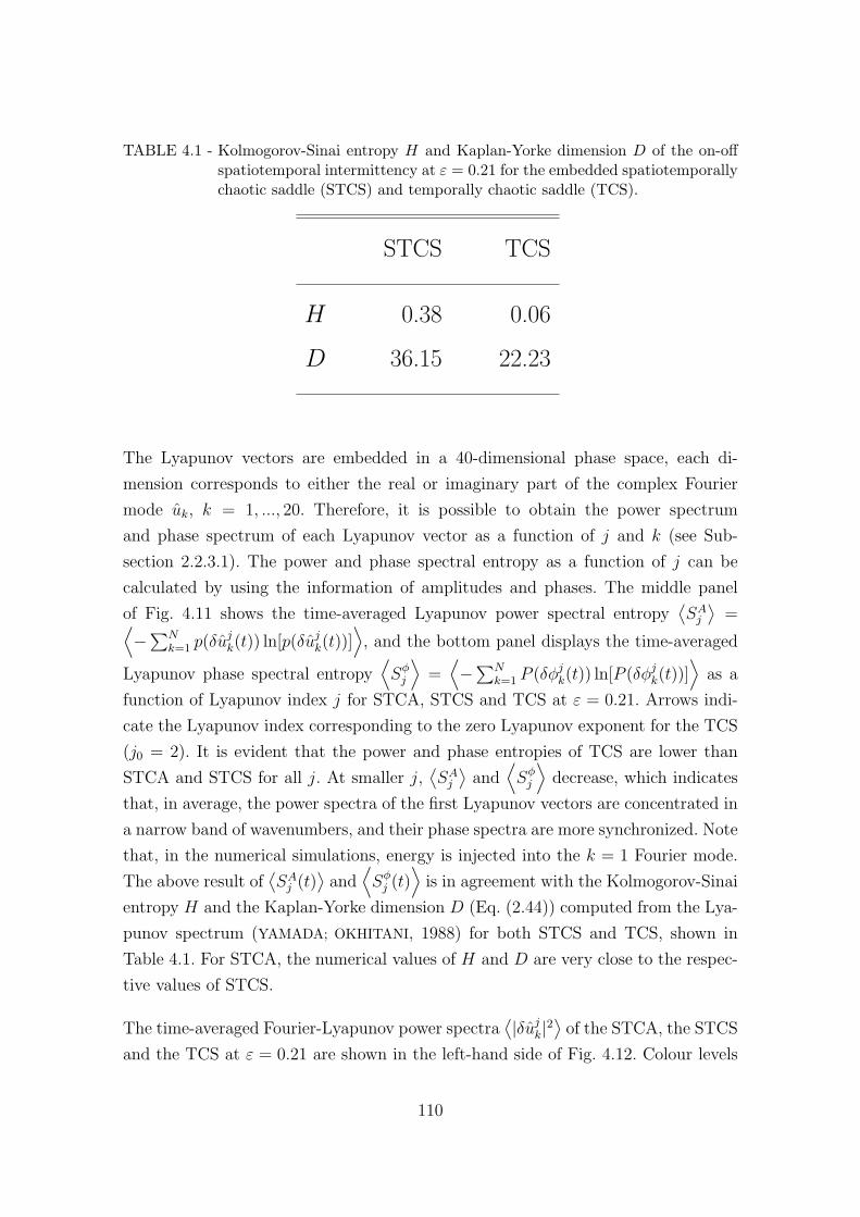
TABLE 4.1 - Kolmogorov-Sinai entropy H and Kaplan-Yorke dimension D of the on-offspatiotemporal intermittency at ε = 0.21 for the embedded spatiotemporallychaotic saddle (STCS) and temporally chaotic saddle (TCS).

STCS TCS

H 0.38 0.06

D 36.15 22.23

The Lyapunov vectors are embedded in a 40-dimensional phase space, each di-

mension corresponds to either the real or imaginary part of the complex Fourier

mode uk, k = 1, ..., 20. Therefore, it is possible to obtain the power spectrum

and phase spectrum of each Lyapunov vector as a function of j and k (see Sub-

section 2.2.3.1). The power and phase spectral entropy as a function of j can be

calculated by using the information of amplitudes and phases. The middle panel

of Fig. 4.11 shows the time-averaged Lyapunov power spectral entropy⟨SAj⟩

=⟨−∑N

k=1 p(δujk(t)) ln[p(δujk(t))]

⟩, and the bottom panel displays the time-averaged

Lyapunov phase spectral entropy⟨Sφj

⟩=⟨−∑N

k=1 P (δφjk(t)) ln[P (δφjk(t))]⟩

as a

function of Lyapunov index j for STCA, STCS and TCS at ε = 0.21. Arrows indi-

cate the Lyapunov index corresponding to the zero Lyapunov exponent for the TCS

(j0 = 2). It is evident that the power and phase entropies of TCS are lower than

STCA and STCS for all j. At smaller j,⟨SAj⟩

and⟨Sφj

⟩decrease, which indicates

that, in average, the power spectra of the first Lyapunov vectors are concentrated in

a narrow band of wavenumbers, and their phase spectra are more synchronized. Note

that, in the numerical simulations, energy is injected into the k = 1 Fourier mode.

The above result of⟨SAj (t)

⟩and

⟨Sφj (t)

⟩is in agreement with the Kolmogorov-Sinai

entropy H and the Kaplan-Yorke dimension D (Eq. (2.44)) computed from the Lya-

punov spectrum (YAMADA; OKHITANI, 1988) for both STCS and TCS, shown in

Table 4.1. For STCA, the numerical values of H and D are very close to the respec-

tive values of STCS.

The time-averaged Fourier-Lyapunov power spectra⟨|δujk|2

⟩of the STCA, the STCS

and the TCS at ε = 0.21 are shown in the left-hand side of Fig. 4.12. Colour levels

110

are indicated in the scales at the bottom of the Figures. For STCA and STCS, j = 15

corresponds to the zero Lyapunov exponent. The Fourier-Lyapunov power spectra of

STCA and STCS display a maximum near the origin of coordinates (j = 0, k = 0).

This means that the first Lyapunov vectors, which are associated with the most

unstable directions, have their energy concentrated at smaller wavenumbers. As a

consequence, there is a strong correspondence between the first Lyapunov vectors

and small wavenumbers, i.e. the Fourier and Lyapunov bases are “frozen” to each

other near the origin (OHKITANI; YAMADA, 1989). Both STCA and STCS have

their energy confined in a narrow inverted-V region in the Fourier-Lyapunov space,

distinct from the Gledzer-Ohkitani-Yamada (GOY) shell model of fully-developed

turbulence where the energy is confined in a narrow V region (YAMADA; OHKITANI,

1998). The power-Lyapunov spectrum of TCS (Fig. 4.12, bottom panel) also shows

a peak near the origin, but the energy spreading is not seen, because the TCS has

only one positive Lyapunov exponent. For all j, the TCS display a higher energy

localization than STCA and STCS, which is in agreement with a low degree of

power spectral entropy as shown in the middle panel of Figure 4.11. Note that

for the TCS, the large energy peaks observed for j > j0 corresponds to negative

Lyapunov exponents, which are related to the dissipation of energy. The smaller

left-hand side panels show the corresponding time-averaged Fourier power spectra

〈|uk|2〉 as a function of wavenumber k, which confirm that the energy bandwidth of

the TCS is narrower than the bandwidth of the STCS and STCA.

The difference between the Fourier-Lyapunov power spectrum of STCA and STCS

shown in Figure 4.12, and the Fourier-Lyapunov power spectrum of the GOY shell

model (YAMADA; OHKITANI, 1998) arises from the way energy injection and dissipa-

tion are modelled. In Yamada and Ohkitani (1998) energy is injected in the fourth

shell, which is analogous to the fourth Fourier mode, whereas the BBM equation

energy is injected into the first Fourier mode. The energy dissipation mechanisms

are also different; Figure 4.13 shows the dissipation term of the BBM equation and

the shell model as a function of wavenumber k.

In addition to the Fourier-Lyapunov power spectrum, the time-averaged phase-

differences spectra⟨δφjk⟩

of STCA, STCS and TCS are displayed in the right-hand

side panels of Fig. 4.12. The Fourier-Lyapunov phase spectra of STCA and STCS

display large peaks of⟨δφjk⟩

corresponding to nonsynchronized modes at all ks and

all js. In contrast, the phase differences spectrum of TCS are small across all ks at

111

0

10

20

j

k

2| u |δ

0 20 30 4010

0 20 30 4010

0 20 30 4010

0.01 0.1

0.01 0.1

0.01 0.1

|u |k

2

(a)

(b)

(c)

(d)

(e)

(f)

δφ jk

0 20 30 4010

0 20 30 4010

0 20 30 4010

0.0 0.004

0.0 0.004

0.0 0.004

kδφ

Fourier Lyapunov power & phase spectra

STCA

j

k

TCS

0

10

20

k

STCS

0

10

20

j

k

0.10.0 0.2

j

STCA

0

10

20

k

j

TCS

0

10

20

k

STCS

0

10

20

k

j

0.10.00.1

j

Amplitude dynamics Phase dynamics

FIGURE 4.12 - Left-hand side panels: Time average of power-Lyapunov spectrum⟨|δujk|

2⟩

of the spatiotemporally chaotic attractor (STCA, top panel),the spatiotemporally chaotic saddle (STCS, middle panel) and the tem-porally chaotic saddle (TCS, bottom panel) at ε = 0.21. Right-hand sidepanels: time average of phase-Lyapunov spectrum of STCA (top panel),STCS (middle panel) and TCS (bottom panel). Fourier wavenumber isindicated by k, and j represent Lyapunov indices. Lyapunov vectors areordered from higher to lower values of their respective Lyapunov expo-nents. The side panels show the time-averaged Fourier power spectra andthe time averaged Fourier phase spectra, respectively.

112

100

101

k

10-4

10-3

10-2

10-1

ν /

(1 −

ak2)

BBM Equation

10-1

100

101

k

10-9

10-6

νk2

GOY Shell Model

FIGURE 4.13 - Dissipation profiles of the Benjamin-Bona-Mahony equation (left sidepanel) and the Shell model of turbulence (right side panel) as a functionof wavenumber k.

low js. Note that the Fourier modes of the unstable Lyapunov vector of TCS (j = 1)

are synchronized, whereas the STCA and STCS display large phase differences for

j < 15, corresponding to unstable Lyapunov vectors. The smaller right-hand side

panels show the plots of the corresponding time-averaged Fourier phase spectra.

These results are in agreement with the bottom panel of Fig. 4.11, in which lower

degree of the phase spectral entropy (i.e. higher degree of synchronization) was ob-

served for the TCS.

113

5 CONCLUSION

In Subsection 3.1 we characterized intermittency and phase synchronization in inter-

mittent magnetic field turbulence. The results presented in subsection 3.1.1 provide

the first observational proof of phase coherence in the ambient solar wind turbu-

lence, based on the magnetic field data of ACE at L1. Figure 3.12 indicates that the

level of intermittency and phase synchronization detected by both Cluster and ACE

are very similar except for scales around 10 s, where ACE observed a higher level of

intermittency and phase synchronization than Cluster. The peak regions of kurtosis

and phase coherence index in Figure 3.12 corresponds to the spectral break regions

in Figure 3.6 where the magnetic field turbulence is dominated by nonlinear wave-

wave and wave-particle interactions. Since Cluster is located in the shocked solar

wind, the reflected ions from the Earth’s bow shock can enhance the dissipation of

nonlinear Alfven waves via ion-cyclotron damping and other kinetic effects (HOWES

et al., 2008), leading to a decrease of phase synchronization.

Our study based on Cluster and ACE observations demonstrate that the intermit-

tency in the magnetic field turbulence, in the shocked solar wind upstream of Earth’s

bow shock and in the unshocked ambient solar wind at L1, is the result of synchro-

nization intrinsic in nonlinear multiscale interactions. Numerical simulations of non-

linear plasma waves have confirmed that intermittent events are localized regions of

plasmas or fluids governed by bursts of energy spikes (coherent structures) where

phase synchronization is operating (HE; CHIAN, 2003; HE; CHIAN, 2005). Since large-

amplitude coherent structures of small scales have typical lifetimes longer than that

of small-amplitude incoherent (stochastic) fluctuations, the dynamics of an intermit-

tent turbulence, ubiquitous in the heliophysical environment (CHIAN et al., 2006), is

dominated by coherent structures resulting from amplitude-phase synchronization.

In subsection 3.1.2 we extended our study presented in subsection 3.1.1 to include an

ICME event observed in January 2005. We analyzed magnetic field measurements

from SOHO MDI solar images, ACE and Cluster data in the solar wind, and ground

magnetometers in Brazil. Finite degree of non-Gaussianity and phase synchroniza-

tion were observed in all datasets. We showed that the interplanetary magnetic field

turbulence downstream of the ICME shock was closely correlated with the Earth’s

geomagnetic turbulence detected on the ground. In a future work we will extend our

analysis of solar images using high-resolution Hinode data, which will allow us to in-

vestigate non-Gaussianity and synchronization at smaller spatial scales than SOHO

115

magnetograms. Some preliminar results are presented in Appendix A (Chapter 7).

The turbulent exchange of mass and momentum from and within canopies is domi-

nated by coherent structures (FINNIGAN, 2000). Wesson et al. (2003) applied three

nonlinear time series techniques (Shannon entropy, wavelet thresholding, and mutual

information content) to contrast the level of organization in vertical wind velocity

in the canopy sublayer and the atmospheric surface layer. In Section 3.2 we have

demonstrated that both kurtosis and phase coherence index techniques are capable

of characterizing the degree of departure from Gaussianity, due to phase coherence,

of atmospheric intermittent turbulence. The nonlinear techniques discussed can be

applied to investigate the role played by coherent structures in experimental (GAO

et al., 1989; BARTHLOTT et al., 2007), theoretical (RAUPACH et al., 1996; HARMAN;

FINNIGAN, 2007), and large-eddy simulation (SU et al., 1998; QIU et al., 2008) studies

of atmospheric turbulence in forest canopy, as well as in orchard canopy (WANG et

al., 1992; STOUGHTON et al., 2002), rice canopy (GAO et al., 2003), corn canopy (YUE

et al., 2007; ZHU et al., 2007), cotton and grape canopies (MITIC et al., 1999), coral

canopy (REIDENBACH et al., 2007), and urban canopy (FEIGENWINTER; VOGT, 2005;

SALMOND et al., 2005).

The theoretical results from numerical simulations of the Benjamin-Bona-Mahony

(BBM) equation (Section 4.1) are consistent with those reported by Rempel et al.

(2007), where the damped Kuramoto-Sivashinsky equation with periodic boundary

conditions was studied. We suggest that the mechanism for the onset of TC-STC

intermittency via the coupling of chaotic saddles can be readily found in other fluid

systems in transition from laminar to weakly turbulent flows, provided the following

conditions are met:

a) There is a discontinuous transition from temporal chaos to spatiotemporal

chaos, due to a crisis-like phenomenon.

b) Before the transition, the system displays transient spatiotemporal chaos.

Examples of fluids with chaotic transients and a crisis transition to spatiotemporal

chaos or turbulence may include the onset of bursting behavior in a driven, two-

dimensional viscous flow subject to no-slip boundaries (MOLENAAR et al., 2007) and

the onset of turbulence in pipe flows. In the latter case, a boundary crisis seems to

be responsible for converting a transient turbulent state into a turbulent attractor at

116

Reynolds ∼ 1800 (WILLIS; KERSWELL, 2007; PEIXINHO; MULLIN, 2006). Although

recent experiments seem to indicate that turbulence in pipe flows is indeed a tran-

sient phenomenon (HOF et al., 2006; HOF et al., 2008), thus contradicting the previous

results. Whether it is transient for all Reynolds numbers or there is a crisis bifurca-

tion to an attractor remains an open question (ECKHARDT, 2008).

In Section 4.2 we used the mathematical tools described in Section 2.2 to measure

the degree of amplitude and phase synchronization in numerical simulations of the

BBM equation after the onset of spatiotemporal chaos. We computed the power-

phase spectral entropies and the power-phase disorder parameters using Fourier and

Lyapunov representations to show that the laminar and bursty periods in the on-

off spatiotemporal intermittency correspond, respectively, to the temporally chaotic

saddle with higher degree of amplitude-phase synchronization and the spatiotem-

porally chaotic saddle with lower degree of amplitude-phase synchronization across

spatial scales.

As a conclusion, the observational results from Chapter 3 indicate that kurtosis

and the phase coherence index display similar variations across scales. The theoret-

ical results from Chapter 4 demonstrates that higher/lower degree of power spec-

tral entropy correspond to higher/lower degree of phase spectral entropies, which

is consistent with our observational results. This duality of amplitude and phase

synchronization may be the origin of intermittency in fully-developed turbulence in

the solar-terrestrial environment.

117

REFERENCES

ABRAMENKO, V.; YURCHYSHYN, V.; WANG, H. Intermittency in the

photosphere and corona above an active region. The Astrophysical Journal,

v. 681, p. 1669–1676, 2008. 135

ABRAMENKO, V. I.; YURCHIYSHIYN, V. B.; WANG, H.; SPIROCK, T. J.;

GOODE, P. R. Scaling behavior of structure functions of the longitudinal magnetic

field in active regions on the sun. The Astrophysical Journal, v. 577, p.

487–495, 2002. 74, 135

ALEXANDROVA, O. Solar wind vs magnetosheath turbulence and Alfven

vortices. Nonlinear Processes in Geophysics, v. 15, p. 95–108, 2008. 63

ALEXANDROVA, O.; CARBONE, V.; VELTRI, P.; SORRISO-VALVO, L. Solar

wind Cluster observations: turbulent spectrum and role of Hall effect. Planetary

and Space Science, v. 55, p. 2224–2227, 2007. 53, 54

. Small-scale energy cascade of the solar wind turbulence. The

Astrophysical Journal, v. 674, p. 1153–1157, 2008. 54, 60, 63, 72, 88

ALLIGOOD, K. T.; SAUER, T. D.; YORKE, J. A. Chaos: an introduction to

dynamical systems. New York: Springer-Verlag, 1996. 35

BADII, R.; POLITI, A. Complexity: hierarchical structures and scaling in

physics. Cambridge: Cambridge University Press, 1997. 97

BALE, S. D.; BALIKHIN, M. A.; HORBURY, T. S.; KRASNOSELSKIKH, V. V.;

KUCHAREK, H.; MOBIUS, E.; WALKER, S. N.; BALOGH, A.; BURGESS, D.;

LEMBEGE, B.; LUCEK, E. A.; SCHOLER, M.; SCHWARTZ, S. J.; THOMSEN,

M. F. Quasi-perpendicular shock structure and processes. Space Science

Reviews, v. 118, p. 161–203, 2005a. 55

BALE, S. D.; KELLOGG, P. J.; MOZER, F. S.; HORBURY, T. S.; REME, H.

Measurement of the electric fluctuation spectrum of magnetohydrodynamic

turbulence. Physical Review Letters, v. 94, n. 215002, 2005b. 53

BALOGH, A.; CARR, C. M.; NA, M. H. A.; DUNLOP, M. W.; BEEK, T. J.;

BROWN, P.; FORNACON, K.-H.; GEORGESCU, E.; GLASSMEIER, K.-H.;

HARRIS, J.; MUSMANN, G.; ODDY, T.; SCHWINGENSCHUH, K. The Cluster

119

magnetic field investigation: overview of in-flight performance and initial results.

Annales Geophysicae, v. 19, p. 1207–1217, 2001. 57

BARTHLOTT, C.; DROBINSKI, P.; FESQUET, C.; DUBOS, T.; PIETRAS, C.

Long-term study of coherent structures in the atmospheric surface layer.

Boundary-Layer Meteorology, v. 125, p. 1–24, 2007. 116

BEHLKE, R.; ANDRE, M.; BALE, S. D.; PICKETT, J. S.; CATTELL, C. A.;

LUCEK, E. A.; BALOGH, A. Solitary structures associated with short

large-amplitude magnetic structures (SLAMS) upstream of the Earth’s

quasi-parallel bow shock. Geophysical Research Letters, v. 31, p. L16805,

2004. 56, 87

BENJAMIN, T. B. The stability of solitary waves. Proceedings of the Royal

Society of London Series A, v. 328, p. 153–183, 1972. 98, 149, 150, 151

BENJAMIN, T. B.; BONA, J. L.; MAHONY, J. J. Model equation for long waves

in nonlinear dispersive systems. Philosophical Transactions of the Royal

Society of London Series A, v. 272, p. 47–78, 1972. 91, 92, 93, 149, 151

BENZI, R.; CILIBERTO, S.; TRIPICCIONE, R.; BAUDET, C.; MASSAIOLI, F.;

SUCCI, S. Extended self-similarity in turbulent flows. Physical Review E, v. 48,

p. R29–R32, 1993. 69

BISKAMP, D. Magnetohydrodynamic turbulence. Cambridge: Cambridge

University Press, 2003. 26, 143

BISKAMP, D.; SCHWARZ, E.; ZEILER, A.; CELANI, A.; DRAKE, J. F.

Electron magnetohydrodynamic turbulence. Physics of Plasmas, v. 6, n. 3, p.

751–758, 1999. 61

BOHR, T.; JENSEN, M. H.; PALADIN, G.; VULPIANI, A. Dynamical systems

approach to turbulence. Cambridge: Cambridge University Press, 1998. 31

BOLZAN, M. J.; RAMOS, F. M.; SA, L. D. A.; NETO, C. R.; ROSA, R. R.

Analysis of fine-scale canopy turbulence within and above an Amazon forest using

Tsallis’ generalized thermostatistics. Journal of Geophysical Research -

Atmospheres, v. 107, n. D20, p. 8063, 2002. 81

120

BOROVSKY, J. E. Flux tube texture of the solar wind: strands of the magnetic

carpet at 1 AU? Journal of Geophysical Research - Space Physics, v. 113,

p. A08110, 2008. 87, 88

BRAUN, R.; FEUDEL, F. Supertransient chaos in the two-dimensional complex

Ginzburg-Landau equation. Physical Review E, v. 53, p. 6562–6565, 1996. 36

BRUNET, P.; LIMAT, L. Defects and spatiotemporal disorder in a pattern of

falling liquid columns. Physical Review E, v. 70, p. 046207, 2004. 98

BRUNO, R.; CARBONE, V. The solar wind as a turbulence laboratory. Living

Reviews in Solar Physics, v. 2, n. 4, 2005. 51, 60

BRUNO, R.; CARBONE, V.; BAVASSANO, B.; SORRISO-VALVO, L.

Observations of magnetohydrodynamic turbulence in the 3D heliosphere.

Advances in Space Research, v. 35, p. 939–950, 2005. 60, 87, 88

BRUNO, R.; CARBONE, V.; SORRISO-VALVO, L.; BAVASSANO, B. Radial

evolution of solar wind intermittency in the inner heliosphere. Journal of

Geophysical Research - Space Physics, v. 108, n. A3, p. 1130, 2003. 57, 86,

87, 88

BRUNO, R.; CARBONE, V.; VELTRI, P.; PIETROPAOLO, E.; BAVASSANO, B.

Identifying intermittency events in the solar wind. Planetary and Space

Science, v. 49, p. 1201–1210, 2001. 87, 88

BURGESS, D.; LUCEK, E. A.; SCHOLER, M.; BALE, S. D.; BALIKHIN, M. A.;

BALOGH, A.; HORBURY, T. S.; KRASNOSELSKIKH, V. V.; KUCHAREK, H.;

LEMBEGE, B.; MOBIUS, E.; SCHWARTZ, S. J.; THOMSEN, M. F.; WALKER,

S. N. Quasi-parallel shock structure and processes. Space Science Reviews,

v. 118, p. 205–222, 2005. 56

BURLAGA, L. F.; VINAS, A. F. Multi-scale probability distributions of solar

wind speed fluctuations at 1 AU described by a generalized Tsallis distribution.

Geophysical Research Letters, v. 31, p. L16807, 2004. 54

CAKMUR, R. V.; EGOLF, D. A.; PLAPP, B. B.; BODENSCHATZ, E. Bistability

and competition of spatiotemporal chaotic and fixed point attractors in

Rayleigh-Benard convection. Physical Review Letters, v. 79, p. 1853–1856,

1997. 39

121

CAMPANHARO, A. S. L. O.; RAMOS, F. M.; MACAU, E. E. N.; ROSA, R. R.;

BOLZAN, M. J. A.; SA, L. D. A. Searching chaos and coherent structures in the

atmospheric turbulence above the Amazon forest. Philosophical Transactions

of the Royal Society of London - Mathematical and Physical Sciences,

v. 366, p. 579–589, 2008. 89

CHANG, T.; TAM, S.; WU, C.-C. Complexity induced anisotropic bimodal

intermittent turbulence in space plasmas. Physics of Plasmas, v. 11, n. 4, p.

1287–1299, 2004. 88

CHAPMAN, S. C.; HNAT, B. Quantifying scaling in the velocity field of the

anisotropic turbulent solar wind. Geophysical Research Letters, v. 34, p.

L17103, 2007. 54

CHATE, H.; MANNEVILLE, P. Transition to turbulence via spatiotemporal

intermittency. Physical Review Letters, v. 58, n. 2, p. 112–115, 1987. 98

CHIAN, A. C.-L.; KAMIDE, Y.; REMPEL, E. L.; SANTANA, W. M. On the

chaotic nature of solar-terrestrial environment: interplanetary Alfven

intermittency. Journal of Geophysical Research - Space Physics, v. 111, n.

A07S03, 2006. 89, 115

CHIAN, A. C.-L.; MIRANDA, R. A. Cluster and ACE observations of phase

synchronization in intermittent magnetic field turbulence: a comparative study of

shocked and unshocked solar wind. Annales Geophysicae, v. 27, p. 1789–1801,

2009. 56, 57, 59, 61, 62, 65, 67, 68, 70, 71, 74, 75, 135

CHIAN, A. C.-L.; MIRANDA, R. A.; KOGA, D.; BOLZAN, M. J. A.; RAMOS,

F. M.; REMPEL, E. L. Analysis of phase coherence in fully developed atmospheric

turbulence: Amazon forest canopy. Nonlinear Processes in Geophysics, v. 15,

p. 567–573, 2008. 33, 51, 69, 70, 80, 81, 82, 83, 84, 85, 86

CHIANG, L.-Y.; COLES, P. Phase information and the evolution of cosmological

density perturbations. Monthly Notices of the Royal Astronomical Society,

v. 311, p. 809–824, 2000. 40

DAUBECHIES, I. Ten lectures on wavelets. Philadelphia: Society for Industrial

and Applied Mathematics (SIAM), 1994. 64

DAVIDSON, P. A. Turbulence: an introduction for scientists and

engineers. New York: Oxford University Press, 2004. 25, 31, 65, 69, 85, 142

122

DE WIT, T. D. Can high-order moments be meaningfully estimated from

experimental turbulence measurements? Physical Review E, v. 70, n. 055302,

2004. 32, 64, 66, 69

DE WIT, T. D.; KRASNOSELSKIKH, V. V. Non-Gaussian statistics in space

plasma turbulence: fractal properties and pitfalls. Nonlinear Processes in

Geophysics, v. 3, p. 262–273, 1996. 66

DODD, R. K.; EILBECK, J. C.; GOBBON, J. D.; MORRIS, H. C. Solitons and

nonlinear wave equations. London: Academic Press, 1982. 91

EASTWOOD, J. P.; BALOGH, A.; LUCEK, E. A.; MAZELLE, C.;

DANDOURAS, I. On the existence of Alfven waves in the terrestrial foreshock.

Annales Geophysicae, v. 21, p. 1457–1465, 2003. 56, 58, 72

ECKHARDT, B. Turbulence transition in pipe flow: some open questions.

Nonlinearity, v. 21, p. T1–T11, 2008. 117

FEIGENWINTER, C.; VOGT, R. Detection and analysis of coherent structures in

urban turbulence. Theoretical and Applied Climatology, v. 81, p. 219–230,

2005. 116

FINNIGAN, J. Turbulence in plant canopies. Annual Review of Fluid

Mechanics, v. 32, p. 519–571, 2000. 116

FOULLON, C.; OWEN, C. J.; DASSO, S.; GREEN, L. M.; DANDOURAS, I.;

ELLIOTT, H. A.; FAZAKERLEY, A. N.; BOGDANOVA, Y. V.; CROOKER,

N. U. Multi-spacecraft study of the 21 january 2005 ICME: evidence of current

sheet substructure near the periphery of a strongly expanding, fast magnetic cloud.

Solar Physics, v. 244, p. 139–165, 2007. 75

FRISCH, U. Turbulence - the legacy of A. N. Kolmogorov. Cambridge:

Cambridge University Press, 1995. 26, 31, 33, 66, 69, 85, 142

FUJISAKA, H.; YAMADA, T. Stability theory of synchronized motion in coupled

oscillator systems. Progress of Theoretical Physics, v. 69, n. 1, p. 32–47, 1983.

45, 47, 104

GAO, W.; SHAW, R. H.; PAW, K. T. Observation of organized structure in

turbulent-flow within and above a forest canopy. Boundary-Layer

Meteorology, v. 47, p. 349–377, 1989. 116

123

GAO, Z.; BIAN, L.; ZHOU, X. Measurements of turbulent transfer in the

near-surface layer over a rice paddy in China. Journal of Geophysical

Research - Atmospheres, v. 108, n. D13, p. 4387, 2003. 116

GRECO, A.; MATTHAEUS, W. H.; SERVIDIO, S.; CHUYCHAI, P.; DMITRUK,

P. Statistical analysis of discontinuities in solar wind ACE data and comparison

with intermittent MHD turbulence. The Astrophysical Journal Letters,

v. 691, p. L111–L114, 2009. 88

HADA, T.; KOGA, D.; YAMAMOTO, E. Phase coherence of MHD waves in the

solar wind. Space Science Reviews, v. 107, p. 463–466, 2003. 33, 51, 55, 69, 70,

74, 82, 135

HAMILTON, K.; SMITH, C. W.; VASQUEZ, B. J.; LEAMON, R. J. Anisotropies

and helicities in the solar wind inertial and dissipation ranges at 1 AU. Journal of

Geophysical Research - Space Physics, v. 113, p. A01106, 2008. 54

HARMAN, I. N.; FINNIGAN, J. J. A simple unified theory for flow in the canopy

and roughness sublayer. Boundary-Layer Meteorology, v. 123, p. 339–363,

2007. 116

HE, K. Crisis-induced transition to spatiotemporally chaotic motions. Physical

Review Letters, v. 80, p. 696–699, 1998. 92, 93, 96, 149

HE, K.; CHIAN, A. C.-L. On-off collective imperfect phase synchronization and

bursts in wave energy in a turbulent state. Physical Review Letters, v. 91, p.

034102, 2003. 26, 40, 51, 89, 92, 96, 115, 149

. Critical dynamic events at the crisis of transition to spatiotemporal chaos.

Physical Review E, v. 69, p. 026207, 2004. 92, 96, 149

. Nonlinear dynamics of turbulent waves in fluids and plasmas. Nonlinear

Processes in Geophysics, v. 12, p. 13–24, 2005. 26, 51, 89, 92, 98, 115, 149

HE, K.; SALAT, A. Hysteresis and onset of chaos in periodically driven nonlinear

drift waves. Plasma Physics and Controlled Fusion, v. 31, p. 123–141, 1989.

92, 93, 98, 149

HOF, B.; DE LOZAR, A.; KUIK, D. J.; WESTERWEEL, J. Repeller or attractor?

Selecting the dynamical model for the onset of turbulence in pipe flow. Physical

Review Letters, v. 101, p. 214501, 2008. 117

124

HOF, B.; WESTERWEEL, J.; SCHNEIDER, T. M.; ECKHARDT, B. Finite

lifetime of turbulence in shear flows. Nature, v. 443, p. 59–62, 2006. 117

HOWES, G. G.; DORLAND, W.; COWLEY, S. C.; HAMMETT, G. W.;

QUATAERT, E.; SCHEKOCHIHIN, A. A.; TATSUNO, T. Kinetic simulations of

magnetized turbulence in astrophysical plasmas. Physical Review Letters,

v. 100, p. 065004, 2008. 115

HSU, G.-H.; OTT, E.; GREBOGI, C. Strange saddles and the dimensions of their

invariant manifolds. Physics Letters A, v. 127, p. 199–204, 1988. 36, 37, 98, 100

KAMIDE, Y.; CHIAN, A. C.-L. Handbook of the Solar-Terrestrial

Environment. Berlin: Springer, 2007. 25, 51

KANTZ, H.; GRASSBERGER, P. Repellers, semi-attractors, and long-lived

chaotic transients. Physica D, v. 17, p. 75–86, 1985. 36, 98

KELLOGG, P. J.; HORBURY, T. S. Rapid density fluctuations in the solar wind.

Annales Geophysicae, v. 23, p. 3765–3773, 2005. 53, 56, 87

KOGA, D.; CHIAN, A. C.-L.; HADA, T.; REMPEL, E. L. Experimental evidence

of phase coherence of magnetohydrodynamic turbulence in the solar wind: Geotail

satellite data. Philosophical Transactions of the Royal Society of London -

Mathematical and Physical Sciences, v. 366, p. 447–457, 2008. 33, 51, 55, 69,

70, 82

KOGA, D.; CHIAN, A. C.-L.; MIRANDA, R. A.; REMPEL, E. L. Intermittent

nature of solar wind turbulence near the Earth’s bow shock: phase coherence and

non-Gaussianity. Physical Review E, v. 75, p. 046401, 2007. 33, 51, 55, 69, 70,

72, 74, 82, 135

KOGA, D.; HADA, T. Phase coherence of foreshock MHD waves: wavelet analysis.

Space Science Review, v. 107, p. 495–498, 2003. 33, 34, 51, 55, 69, 70

KOLMOGOROV, A. N. C. R. Acad. Nauk. SSSR, v. 98, p. 527, 1941. 25, 30

KULKARNI, J. R.; SADANI, L. K.; MURTHY, B. S. Wavelet analysis of

intermittent turbulent transport in the atmospheric surface layer over a Monsoon

trough region. Boundary-Layer Meteorology, v. 90, p. 217–239, 1999. 81

125

KURAMOTO, Y. Chemical oscillations, waves and turbulence. Berlin:

Springer-Verlag, 1984. 41

LAI, Y.-C.; BOLLT, E. M.; LIU, Z. Low-dimensional chaos in high-dimensional

phase space: how does it occur? Chaos, Solitons and Fractals, v. 15, p.

219–232, 2003. 45, 47

LAI, Y.-C.; FREI, M. G.; OSORIO, I. Detecting and characterizing phase

synchronization in nonstationary dynamical systems. Physical Review E, v. 73,

p. 026214, 2006. 40

LANGHANS, K.; SCHMIDT, W. Center-to-limb variation of the G-band lines at

430.5 nm. Astronomy and Astrophysics, v. 382, n. 1, p. 312–318, 2001. 135

LEAMON, R. J.; MATTHAEUS, W. H.; SMITH, C. W.; ZANK, G. P.; MULLAN,

D. J.; OUGHTON, S. MHD-driven kinetic dissipation in the solar wind and

corona. The Astrophysical Journal, v. 537, p. 1054–1062, 2000. 60

LUCEK, E. A.; HORBURY, T. S.; BALOGH, A.; DANDOURAS, I.; REME, H.

Cluster observations of structures at quasi-parallel bow shocks. Annales

Geophysicae, v. 22, p. 2309–2314, 2004. 56, 87

MACEK, W. M. Testing for an attractor in the solar wind flow. Physica D,

v. 122, p. 254–264, 1998. 89

MACEK, W. M.; BRUNO, R.; CONSOLINI, G. Generalized dimensions for

fluctuations in the solar wind. Physical Review E, v. 72, p. 017202, 2005. 60

MANSCHER, M.; NORDAHN, M.; MOSEKILDE, E.; MAISTRENKO, L. Riddled

basins of attraction for synchronized type-I intermittency. Physical Letters A,

v. 238, p. 358–364, 1998. 47

MARTIN, D. U.; YUEN, H. C. Spreading of energy in solutions of the nonlinear

Schrodinger equation. Physics of Fluids, v. 23, p. 1269–1271, 1980. 40

MATTHAEWS, W. H.; GOLDSTEIN, M. L.; C., S. Evaluation of magnetic

helicity in homogeneous turbulence. Physical Review Letters, v. 48, p.

1256–1259, 1982. 25

MCCOMAS, D. J.; BAME, S. J.; BARKER, P.; FELDMAN, W. C.; PHILLIPS,

J. L.; RILEY, P.; GRIFFEE, J. W. Solar Wind Electron Proton Alpha Monitor

126

(SWEPAM) for the Advanced Composition Explorer. Space Science Review,

v. 86, p. 563–612, 1998. 60

MIRANDA, R. A.; CHIAN, A. C.-L.; DASSO, S.; ECHER, E.; MUNOZ, P. R.;

TRIVEDI, N. B.; TSURUTANI, B. T.; YAMADA, M. Observation of

non-Gaussianity and phase synchronization in intermittent magnetic field

turbulence in the solar-terrestrial environment. In: INTERNATIONAL

ASTONOMICAL UNION, IAUS264., 2009, Rio de Janeiro, Brazil. Proceedings

IAU Symposium No. 264, 2009. Cambridge: Cambridge University Press,

2009. p. 363–368. ISBN 978-0-521-76499-5. 73, 76, 77

MITIC, C. M.; MASSMAN, W. J.; SCHUEPP, P. H.; COLLETT JR., J. L.

Structural analysis and flux associations of CO2, H2O, heat and ozone over cotton

and grape canopies. Atmospheric Environment, v. 33, p. 1159–1173, 1999. 116

MOLENAAR, D.; CLERCX, H. J. H.; VAN HEIJST, G. J. F. Attractor crisis and

bursting in a fluid flow with two no-slip directions. Physical Review E, v. 75, p.

036309, 2007. 116

MONIN, A. S.; YAGLOM, A. M. Statistical fluid mechanics volume 1. [S.l.]:

Dover Publications, 1971. 30, 32

NARITA, Y.; GLASSMEIER, K.-H.; TREUMANN, R. A. Wave-number spectra

and intermittency in the terrestrial foreshock region. Physical Review Letters,

v. 97, p. 191101, 2006. 53

NARIYUKI, Y.; HADA, T. Remarks on nonlinear relation among phases and

frequencies in modulational instabilities of parallel propagating Alfven waves.

Nonlinear Processes in Geophysics, v. 13, p. 425–441, 2006. 33, 69, 70

NARIYUKI, Y.; HADA, T.; TSUBOUCHI, K. On nonlinear evolution of Alfvenic

turbulence in low beta plasmas. Physics of Plasmas, v. 15, p. 114502, 2008. 33,

69, 70

NICHOLSON, D. R. Introduction to plasma theory. New York: John Wiley &

Sons, 1983. 91

OHKITANI, K.; YAMADA, M. Temporal intermittency in the energy cascade

process and local Lyapunov analysis in fully-developed model turbulence.

Progress of Theoretical Physics, v. 81, p. 329–341, 1989. 40, 111

127

OTT, E. Chaos in dynamical systems. Cambridge: Cambridge University

Press, 1993. 37, 43

OUELLETTE, N. T.; GOLLUB, J. P. Dynamic topology in spatiotemporal chaos.

Physics of Fluids, v. 20, p. 064104, 2008. 36

PALLOCCHIA, G.; BRUNO, R.; BAVASSANO, B.; et al. Turbulence in the solar

wind as seen by Cluster CIS experiment: Preliminary results on intermittency and

scaling laws. In: SOLSPA 2001, Proceedings of the Second Solar Cycle

and Space Weather Euroconference. [S.l.]: ESA Special Publication, 2002. p.

361–364. 53

PAPOULIS, A. Probability, random variables, and stochastic processes.

New York: McGraw-Hill, 1965. 65

PARKER, T. S.; CHUA, L. O. Practical numerical algorithms for chaotic

systems. New York: Springer-Verlag, 1989. 42, 43

PARKS, G. K.; LEE, E.; MOZER, F.; WILBER, M.; LUCEK, E.; DANDOURAS,

I.; REME, H.; MAZELLE, C.; CAO, J. B.; MEZIANE, K.; GOLDSTEIN, M. L.;

ESCOUBET, P. Larmor radius size density holes discovered in the solar wind

upstream of Earth’s bow shock. Physics of Plasmas, v. 13, p. 050701, 2006. 87

PASCHMANN, G.; DALY, P. W. Analysis methods for multi-spacecraft

data. The Netherlands: ESA Publications Division, 2000. 60, 61

PEIXINHO, J.; MULLIN, T. Decay of turbulence in pipe flow. Physical Review

Letters, v. 96, p. 094501, 2006. 117

PEREGRINE, D. H. Calculations of the development of an undular bore. Journal

of Fluid Mechanics, v. 25, p. 321–330, 1966. 92

PETZOLD, L. R. Automatic selection of methods for solving stiff and nonstiff

systems of ordinary differential equations. SIAM Journal of Scientific

Statistics and Computation, v. 4, p. 136–148, 1983. 94

PLATT, N.; SPIEGEL, E. A.; TRESSER, C. On-off intermittency: a mechanism

for bursting. Physical Review Letters, v. 70, n. 3, p. 279–282, 1993. 47

POLITANO, H.; POUQUET, A. von-Karman-Howarth equation for

magnetohydrodynamics and its consequences on third-order longitudinal structure

and correlation functions. Physical Review E, v. 57, p. R21–R24, 1998. 142, 143

128

POLYGIANNAKIS, J. M.; MOUSSAS, X. Detection of nonlinear dynamics in

solar wind and a comet using phase-correlation measures. Solar Physics, v. 158,

p. 159–172, 1995. 40

POWELL, G. E.; PERCIVAL, I. C. A spectral entropy method for distinguishing

regular and irregular motion of hamiltonian systems. Journal of Physics A:

Mathematical and General, v. 12, p. 2053–2071, 1979. 39, 96

QIU, J.; GU, Z. L.; WANG, Z. S. Numerical study of the response of an

atmospheric surface layer to a spatially nonuniform plant canopy.


RAMOS, F. M.; BOLZAN, M. J. A.; SA, L. D. A.; ROSA, R. R. Atmospheric

turbulence within and above an Amazon forest. Physica D, v. 193, p. 278–291,

2004. 81

RAUPACH, M. R.; FINNIGAN, J. J.; BRUNET, Y. Coherent eddies and

turbulence in vegetation canopies: the mixing-layer analogy. Boundary-Layer

Meteorology, v. 78, p. 351–382, 1996. 116

REIDENBACH, M. A.; KOSEFF, J. R.; MONISMITH, S. G. Laboratory

experiments of fine-scale mixing and mass transport within a coral canopy.

Physics of Fluids, v. 19, p. 075107, 2007. 116

REME, H.; AOUSTIN, C.; et al. First multispacecraft ion measurements in and

near the Earth’s magnetosphere with the identical Cluster Ion Spectrometry (CIS)

experiment. Annales Geophysicae, v. 19, p. 1303–1354, 2001. 60

REMPEL, E. L.; CHIAN, A. C.-L. Origin of transient and intermittent dynamics

in spatiotemporal chaotic systems. Physical Review Letters, v. 98, p. 014101,

2007. 37, 89, 92, 93, 100, 102, 103, 149

REMPEL, E. L.; CHIAN, A. C.-L.; MACAU, E. E. N.; ROSA, R. R. Analysis of

chaotic saddles in low-dimensional dynamical systems: the derivative nonlinear

Schrodinger equation. Physica D, v. 199, p. 407–424, 2004. 36, 37

REMPEL, E. L.; CHIAN, A. C.-L.; MIRANDA, R. A. Chaotic saddles at the onset

of intermittent spatiotemporal chaos. Physical Review E, v. 76, p. 056217, 2007.

37, 89, 93, 96, 98, 100, 103, 116

129

REMPEL, E. L.; MIRANDA, R. A.; CHIAN, A. C.-L. Spatiotemporal

intermittency and chaotic saddles in the regularized long-wave equation. Physics

of Fluids, v. 21, p. 074105, 2009. 95, 96, 97, 99, 101, 102, 103

SAHRAOUI, F. Diagnosis of magnetic structures and intermittency in

space-plasma turbulence using the technique of surrogate data. Physical Review

E, v. 78, p. 026402, 2008. 33, 51, 55, 69, 70

SALMOND, J. A.; OKE, T. R.; GRIMMOND, C. S. B.; ROBERTS, S.;

OFFERLE, B. Venting of heat and carbon dioxide from urban canyons at night.

Journal of Applied Meteorology, v. 44, p. 1180–1194, 2005. 116

SAMSONOV, A. A.; ALEXANDROVA, O.; LACOMBE, C.; MAKSIMOVIC, M.;

GARY, S. P. Proton temperature anisotropy in the magnetosheath: comparison of

3-D MHD modelling with Cluster data. Annales Geophysicae, v. 25, p.

1157–1173, 2007. 63

SCHWARTZ, S. J. Shocks: commonalities in solar-terrestrial chains. Space

Science Review, v. 124, p. 333–344, 2006. 87

SHANNON, C. E. A mathematical theory of communication. Bell System

Technical Journal, v. 27, p. 379–423, 1949. 39, 145

SHIMADA, I.; NAGASHIMA, T. A numerical approach to ergodic problem of

dissipative dynamical systems. Progress of Theoretical Physics, v. 61, p.

1605–1616, 1979. 43, 108

SILVA DIAS, M. A. F.; RUTLEDGE, S.; KABAT, P.; DIAS, P. L. S.; NOBRE, C.;

FISCH, G.; DOLMAN, A. J.; ZIPSER, E.; GARSTANG, M.; MANZI, A. O.;

FUENTES, J. D.; ROCHA, H. R.; MARENGO, J.; PLANA-FATTORI, A.; SA, L.

D. A.; ALVALA, R. C. S.; ANDREAE, M. O.; ARTAXO, P.; GIELOW, R.;

GATTI, L. Cloud and rain processes in a biosphere-atmosphere interaction context

in the Amazon region. Journal of Geophysical Research - Atmospheres,

v. 107, n. D20, p. 8072, 2002. 79

SMITH, C. W.; HAMILTON, K.; VASQUEZ, B. J.; LEAMON, R. J. Dependence

of the dissipation range spectrum of interplanetary magnetic fluctuations on the

rate of energy cascade. The Astrophysical Journal Letters, v. 645, p.

L85–L88, 2006. 54

130

SMITH, C. W.; L’HEUREUX, J.; NESS, N. F.; NA, M. H. A.; BURLAGA, L. F.;

SCHEIFELE, J. The ACE magnetic fields experiment. Space Science Review,

v. 86, p. 613–632, 1998. 57

STASIEWICZ, K.; LONGMORE, M.; BUCHERT, S.; SHUKLA, P. K.;

LAVRAUD, B.; PICKETT, J. Properties of fast magnetosonic shocklets at the

bow shock. Geophysical Research Letters, v. 30, n. 24, p. 2241, 2003. 56, 87

STOUGHTON, T. E.; MILLER, D. R.; HUDDLESTON, E. W.; ROSS, J. B.

Evapotranspiration and turbulent transport in an irrigated desert orchard.

Journal of Geophysical Research - Atmosphere, v. 107, p. 4425, 2002. 116

SU, H.-B.; SHAW, R. H.; U, K. T. P.; MOENG, C.-H.; SULLIVAN, P. P.

Turbulent statistics of neutrally stratified flow within and above a sparse forest

from large-eddy simulation and field observations. Boundary-Layer

Meteorology, v. 88, p. 363–397, 1998. 116

SWEET, D.; NUSSE, H. E.; YORKE, J. A. Stagger-and-step method: detecting

and computing chaotic sadddles in higher dimensions. Physical Review Letters,

v. 86, p. 2261–2264, 2001. 37, 38, 107

TAJIMA, T. Computational plasma physics: with applications to fusion

and astrophysics. Massachusetts: Addison-Wesley, 1989. 94

TAN, C.; CHEN, P. F.; ABRAMENKO, V.; WANG, H. Evolution of optical

penumbral and shear flows associated with the X3.4 flare of 2006 december 13.

The Astrophysical Journal, v. 690, p. 1820–1828, 2009. 135

TASS, P.; ROSENBLUM, M. G.; WEULE, J.; KURTHS, J.; PIKOVSKY, A.;

VOLKMANN, J.; SCHNITZLER, A.; FREUND, H.-J. Detection of n:m phase

locking from noisy data: application to magnetoencephalography. Physical

Review Letters, v. 81, p. 3291–3294, 1998. 40

TAYLOR, G. I. The spectrum of turbulence. Proceedings of the Royal Society

of London A, v. 164, p. 476–490, 1938. 31

TEL, T.; LAI, Y.-C. Chaotic transients in spatially extended systems. Physics

Reports, v. 460, p. 245–275, 2008. 36

131

TELLONI, D.; ANTONUCCI, E.; BRUNO, R.; D’AMICIS, R. Persistent and

self-similar large-scale density fluctuations in the solar corona. The

Astrophysical Journal, v. 693, p. 1022–1028, 2009. 33, 51, 69, 70

THYAGARAJA, A. Recurrent motions in certain continuum dynamical systems.

Physics of Fluids, v. 22, p. 2093–2096, 1979. 40

TSUNETA, S.; ICHIMOTO, K.; et al. The solar optical telescope for the Hinode

mission: an overview. Solar Physics, v. 249, n. 2, p. 167–196, 2008. 135

VELTRI, P. MHD turbulence in the solar wind: self-similarity, intermittency and

coherent structures. Plasma Physics and Controlled Fusion, v. 41, p.

A787–A795, 1999. 88

VELTRI, P.; MANGENEY, A. Scaling laws and intermittent structures in solar

wind MHD turbulence. Solar Wind Nine, p. 543–546, 1999. 88

WANG, Y. S.; MILLER, D. R.; ANDERSON, D. E.; CIONCO, R. M.; LIN, J. D.

A spatial length scale analysis of turbulent temperature and velocity fluctuations

within and above an orchard canopy. Boundary-Layer Meteorology, v. 59, p.

125–139, 1992. 116

WELCH, P. The use of fast Fourier transform for the estimation of power spectra:

a method based on time averaging over short, modified periodograms. IEEE

Transactions Audio and Electroacoustics, AU-15, n. 2, p. 70–73, 1967. 60

WESSON, K. H.; KATUL, G. G.; SIQUEIRA, M. Quantifying organization of

atmospheric turbulent eddy motion using nonlinear time series analysis.


WILLIS, A. P.; KERSWELL, R. R. Critical behavior in the relaminarization of

localized turbulence in pipe flow. Physical Review Letters, v. 98, p. 014501,

2007. 117

WOLF, A.; SWIFT, J. B.; SWINNEY, H. L.; VASTANO, J. A. Determining

Lyapunov exponents from a time series. Physica D, v. 16, p. 285–317, 1985. 94

XI, H.; GUNTON, J. D. Spatiotemporal chaos in a model of Rayleigh-Benard

convection. Physical Review E, v. 52, p. 4963–4975, 1995. 39, 96

132

YAMADA, M.; OHKITANI, K. Asymptotic formulas for the Lyapunov spectrum

of fully developed shell model turbulence. Physical Review E, v. 57, p.

R6257–R6260, 1998. 43, 108, 111

YAMADA, M.; OKHITANI, K. Lyapunov spectrum of a model of two-dimensional

turbulence. Physical Review Letters, v. 60, n. 11, p. 983–986, 1988. 108, 110

YAMADA, M.; SAIKI, Y. Chaotic properties of a fully developed model

turbulence. Nonlinear Processes in Geophysics, v. 14, p. 631–640, 2007. 43

YUE, W.; PARLANGE, M. B.; MENEVEAU, C.; ZHU, W.; VAN HOUT, R.;

KATZ, J. Large-eddy simulation of plant canopy flows using plant-scale

representation. Boundary-Layer Meteorology, v. 124, p. 183–203, 2007. 116

ZHOU, Y.; MATTHAEUS, W. H.; DMITRUK, P. Magnetohydrodynamic

turbulence and time scales in astrophysical and space plasmas. Reviews Modern

Physics, v. 76, p. 1015–1035, 2004. 88

ZHU, W.; VAN HOUT, R.; KATZ, J. PIV measurements in the atmospheric

boundary layer within and above a mature corn canopy. Part II: Quadrant-hole

analysis. Journal of Atmospheric Science, v. 64, p. 2825–2838, 2007. 116

133

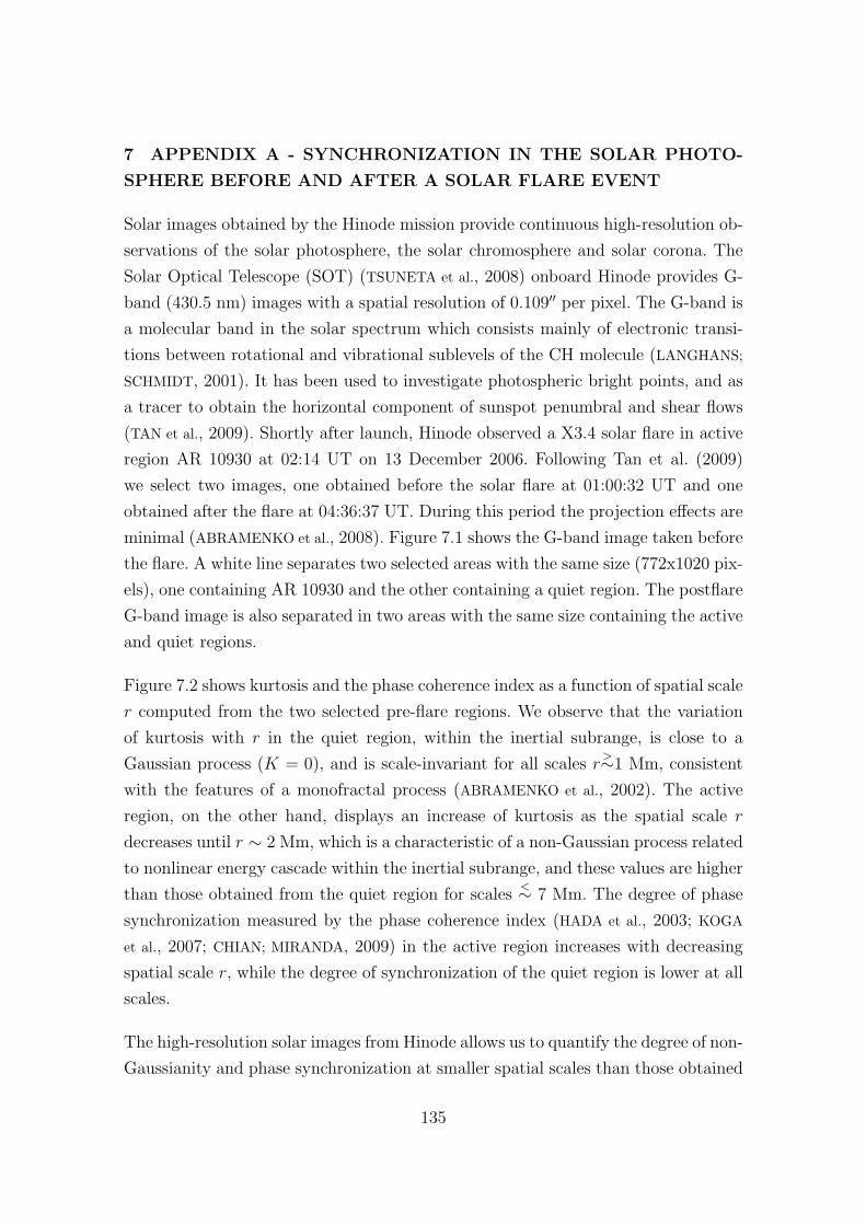
7 APPENDIX A - SYNCHRONIZATION IN THE SOLAR PHOTO-

SPHERE BEFORE AND AFTER A SOLAR FLARE EVENT

Solar images obtained by the Hinode mission provide continuous high-resolution ob-

servations of the solar photosphere, the solar chromosphere and solar corona. The

Solar Optical Telescope (SOT) (TSUNETA et al., 2008) onboard Hinode provides G-

band (430.5 nm) images with a spatial resolution of 0.109′′ per pixel. The G-band is

a molecular band in the solar spectrum which consists mainly of electronic transi-

tions between rotational and vibrational sublevels of the CH molecule (LANGHANS;

SCHMIDT, 2001). It has been used to investigate photospheric bright points, and as

a tracer to obtain the horizontal component of sunspot penumbral and shear flows

(TAN et al., 2009). Shortly after launch, Hinode observed a X3.4 solar flare in active

region AR 10930 at 02:14 UT on 13 December 2006. Following Tan et al. (2009)

we select two images, one obtained before the solar flare at 01:00:32 UT and one

obtained after the flare at 04:36:37 UT. During this period the projection effects are

minimal (ABRAMENKO et al., 2008). Figure 7.1 shows the G-band image taken before

the flare. A white line separates two selected areas with the same size (772x1020 pix-

els), one containing AR 10930 and the other containing a quiet region. The postflare

G-band image is also separated in two areas with the same size containing the active

and quiet regions.

Figure 7.2 shows kurtosis and the phase coherence index as a function of spatial scale

r computed from the two selected pre-flare regions. We observe that the variation

of kurtosis with r in the quiet region, within the inertial subrange, is close to a

Gaussian process (K = 0), and is scale-invariant for all scales r>∼1 Mm, consistent

with the features of a monofractal process (ABRAMENKO et al., 2002). The active

region, on the other hand, displays an increase of kurtosis as the spatial scale r

decreases until r ∼ 2 Mm, which is a characteristic of a non-Gaussian process related

to nonlinear energy cascade within the inertial subrange, and these values are higher

than those obtained from the quiet region for scales<∼ 7 Mm. The degree of phase

synchronization measured by the phase coherence index (HADA et al., 2003; KOGA

et al., 2007; CHIAN; MIRANDA, 2009) in the active region increases with decreasing

spatial scale r, while the degree of synchronization of the quiet region is lower at all

scales.

The high-resolution solar images from Hinode allows us to quantify the degree of non-

Gaussianity and phase synchronization at smaller spatial scales than those obtained

135

AR 10930 Quiet region

454 504 554 604

40

60

80

100

120

140

S−

N (

arcs

econ

d)

E−W (arcsecond)

Hinode SOT G−band at 01:00:32 UT on 13 December 2006

FIGURE 7.1 - Hinode SOT G-band image taken at 01:00:32 UT on 13 December 2006.The white line separates two areas containing the active region AR 10930,and a quiet region.

from solar images from SOHO. Fig. 7.2 shows that the degree of non-Gaussianity

and synchronization of AR 10930 and the quiet region increases for scales r<∼1 Mm,

which indicates that both regions display intermittent features for r<∼1.

Next we compare the degree of amplitude and phase synchronization of the active

region before and after the flare. Figure 7.3 shows kurtosis and the phase coherence

index as a function of spatial scale r computed from AR 10930 before (continuous

line) and after (dashed line) the solar flare. The degree of intermittency and syn-

chronization in the active region is almost the same before and after the flare, being

only slightly higher at scales r>∼1 before the solar flare. The degree of phase syn-

chronization measured by the phase coherence index is consistent with the variation

of kurtosis.

136

0

1

2

3

4

Kurt

osi

s


Before flare

10-1

100

101

r (Mm)

0

0.2

0.4

Phas

e co

her

ence

index

FIGURE 7.2 - Kurtosis (upper panel) and the phase coherence index (lower panel) as afunction of spatial scale r computed from AR 10930 (black line) and thequiet region (grey line) before the solar flare.

0

1

2

3

4

Kurt

osi

s

Before flare After flare

AR 10930

10-1

100

101

r (Mm)

0

0.2

0.4

Phas

e co

her

ence

index

FIGURE 7.3 - Kurtosis (upper panel) and the phase coherence index (lower panel) as afunction of spatial scale r computed from AR 10930 before (black line) andafter (dashed line) the solar flare.

137

8 APPENDIX B - KOLMOGOROV 1941 THEORY AND ITS EXTEN-

SION TO MAGNETOHYDRODYNAMICS

8.1 Neutral fluids

The dynamics of incompressible, neutral fluids can be described by the Navier-Stokes

equations

∂tu + (u · ∇)u = −∇p+ ν∆u + f , (8.1)

∇ · u = 0. (8.2)

where u = u(x, t) denotes the fluid velocity which depends on position x and time

t, p is the pressure, ν represents the kinematic viscosity, and f is an external force.

Let us define u1 as the i-th component of the fluid velocity at point x1 and u2 as

the j-th component of the velocity at point x2 separated from point x1 by a distance

|r| = r. Rewriting Equation (8.1)

∂tu1i + ∂1ku1ku1i = −∂1ip+ ν∆1u1i + f1i, (8.3)

∂tu2j + ∂2ku2ku2j = −∂2jp+ ν∆1u2j + f2j, (8.4)

where we have made use of Einstein’s notation. Next, we multiply Equation (8.3) by

u2j and equation (8.4) by u1i, sum the two resulting equations and take the average

∂t 〈u1iu2j〉+ ∂1k 〈u2ju1ku1i〉+ ∂2k 〈u1iu2ku2j〉

= −∇1i 〈u2jp〉 − ∇2j 〈u1ip〉+ ν∆1 〈u2ju1i〉+ ν∆2 〈u1iu2j〉

+ 〈u1if2j〉+ 〈u2jf1i〉 , (8.5)

where the 〈〉 denote the ensemble average. Let us define the correlation functions

139

〈u1iu2j〉 = Cij(r), (8.6)

〈u1iu1ku2j〉 = Cik,j(r), (8.7)

and partial derivatives

∂1k = −∂rk , (8.8)

∂2k = ∂rk . (8.9)

Equation (8.5) can be written as

∂tCij(r) = ∂rkCik,j(r) + ∂rkCjk,i(r) + 2ν∆Cij(r) + 2εij(r), (8.10)

where εij is a tensor related to energy dissipation rate. Taking the trace of equation

(8.10) and integrating with respect to rk one obtains

Cik,i(r) + ν∂rkCii(r) = −1

3εrk. (8.11)

where ε is the mean energy dissipation rate. Let us define the second and third-order

two-point differences as

S2(r) =⟨(δu1)

2⟩,

S3(r) =⟨(δu1)

3⟩,

where δu1(r) = u1(x1 + r)− u1(x1). Assuming homogeneity and isotropy, the corre-

lation functions are related to two-point differences (or structure functions) by the

following identities

140

Cii(r) =1

2r2∂rr

3S2(r), (8.12)

Cik,i(r) =1

12

rkr3∂rr

4S3(r). (8.13)

Inserting (8.12) and (8.13) into (8.11) one obtains

S3(r)− ν∂rS2(r) = −4

5εr. (8.14)

In the limit ν → 0

S3(r) = −4

5εr. (8.15)

where r = |r| represents spatial scale. Equation (8.15) was obtained by Kolmogorov

in 1941. By assuming that turbulence is self-similar at small scales, i. e. it posesses

a unique scaling exponent

δu(λr) = λαδu(r). (8.16)

Subtituting (8.16) into (8.15)

λ3αS3 = −4

5ελr, (8.17)

hence the scaling exponent should be equal to 1/3.

Eq. (8.15) can be generalized to structure functions of order p

Sp(r) = 〈(δu)p〉 . (8.18)

From the self-similarity assumption we can infer that, if S3 ∝ r for p = 3, then in

general Sp ∝ rαp = rp/3, and since (εr)p/3 has exactly the same dimensions as Sp for

141

p = 3, the structure function of order p should obey (FRISCH, 1995)

Sp = Cpεp/3rp/3, (8.19)

where Cp is a dimensionless constant. For p = 3, Cp = −4/5.

The second-order structure function is related with the energy spectrum by (DAVID-

SON, 2004)

⟨(δu(r))2⟩ ∼ ∫ ∞

π/r

E(k)dk, (8.20)

where E(k) represents the energy of eddies of size r ∼ π/k. Combining Eq. (8.20)

with Eq. (8.19) with p = 2, and taking the derivative with respect to k one can

obtain

E(k) ∼ C ′2ε2/3k−5/3, (8.21)

where C ′2 = −(2C2π2/3)/3.

8.2 Magnetized flows

A similar derivation for turbulent magnetized flows was carried out by Politano and

Pouquet (1998). The magnetohydrodinamical (MHD) equations which govern the

dynamics of incompressible conducting flows can be written in terms of Elsasser

variables as

(∂t + z∓ · ∇

)z± = −∇P∗ + ν+∇2z± + ν−∇2z∓, (8.22)

∇ · u = 0, (8.23)

∇ · b = 0, (8.24)

where z± = u ± b represent the Elsasser variable, b is the magnetic field, P∗ =

P + |b|2/2 is the total pressure, and ν± = (ν ± η)/2 where ν is the viscosity and η

142

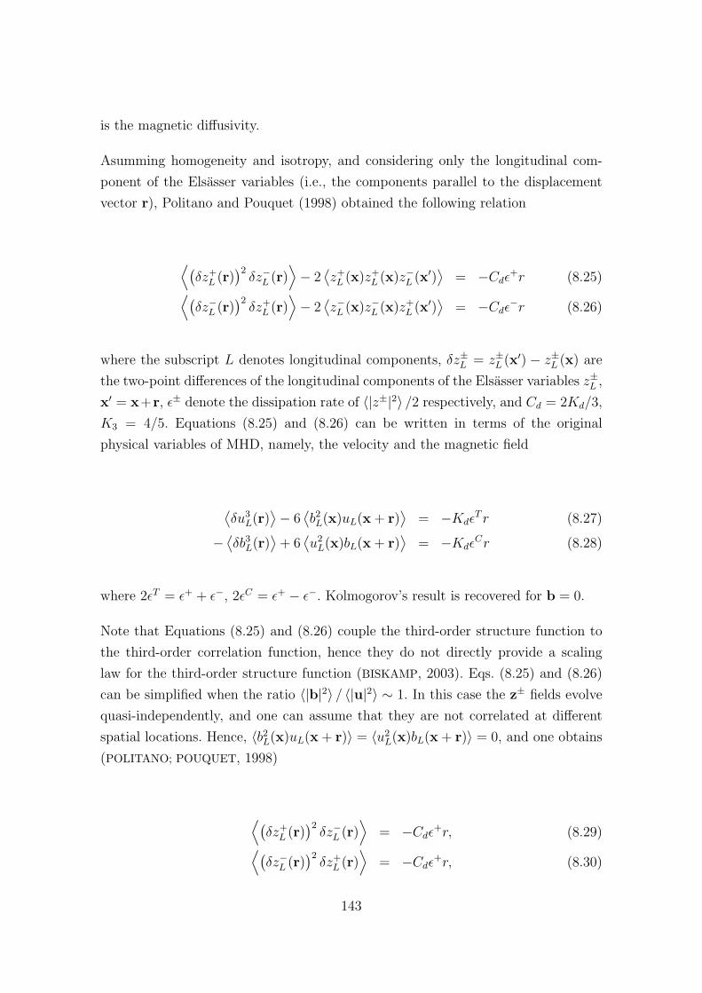
is the magnetic diffusivity.

Asumming homogeneity and isotropy, and considering only the longitudinal com-

ponent of the Elsasser variables (i.e., the components parallel to the displacement

vector r), Politano and Pouquet (1998) obtained the following relation

⟨(δz+

L (r))2δz−L (r)

⟩− 2

⟨z+L (x)z+

L (x)z−L (x′)⟩

= −Cdε+r (8.25)⟨(δz−L (r)

)2δz+L (r)

⟩− 2

⟨z−L (x)z−L (x)z+

L (x′)⟩

= −Cdε−r (8.26)

where the subscript L denotes longitudinal components, δz±L = z±L (x′) − z±L (x) are

the two-point differences of the longitudinal components of the Elsasser variables z±L ,

x′ = x+r, ε± denote the dissipation rate of 〈|z±|2〉 /2 respectively, and Cd = 2Kd/3,

K3 = 4/5. Equations (8.25) and (8.26) can be written in terms of the original

physical variables of MHD, namely, the velocity and the magnetic field

⟨δu3

L(r)⟩− 6

⟨b2L(x)uL(x + r)

⟩= −Kdε

T r (8.27)

−⟨δb3L(r)

⟩+ 6

⟨u2L(x)bL(x + r)

⟩= −Kdε

Cr (8.28)

where 2εT = ε+ + ε−, 2εC = ε+ − ε−. Kolmogorov’s result is recovered for b = 0.

Note that Equations (8.25) and (8.26) couple the third-order structure function to

the third-order correlation function, hence they do not directly provide a scaling

law for the third-order structure function (BISKAMP, 2003). Eqs. (8.25) and (8.26)

can be simplified when the ratio 〈|b|2〉 / 〈|u|2〉 ∼ 1. In this case the z± fields evolve

quasi-independently, and one can assume that they are not correlated at different

spatial locations. Hence, 〈b2L(x)uL(x + r)〉 = 〈u2L(x)bL(x + r)〉 = 0, and one obtains

(POLITANO; POUQUET, 1998)

⟨(δz+

L (r))2δz−L (r)

⟩= −Cdε+r, (8.29)⟨(

δz−L (r))2δz+

L (r)⟩

= −Cdε+r, (8.30)

143

which are closer to Kolmogorov’s law shown in Eq. (8.15). In terms of velocity and

magnetic fields, Eqs. (8.29) and (8.30) read

⟨δu3

L(r)⟩−⟨δuL(r)δb2L(r)

⟩= −Kdε

T r, (8.31)

−⟨δb3L(r)

⟩+⟨δbL(r)δu2

L(r)⟩

= −KdεT r, (8.32)

144

9 APPENDIX C - SHANNON ENTROPY

In this Appendix we derive the Shannon entropy following the original derivation

by Shannon (1949). Let H = H(p1, p2, ..., pn) denote the “amount of uncertainty”

(entropy) of a specific process. We make the following assumptions:

a)H should be continuous in pi.

b)If all pi are equal, pi = 1/N , then H should be a monotonic increasing func-

tion of N (with equally likely events there is more choice, or uncertainty,

when there are more possible events).

c)If a choice is decomposed into two successive choices, then the original H

should be the weighted sum of the individual values of H. For example,

in Figure 9.1, we can decompose three possibilities p1 = 1/2, p2 = 1/3

and p3 = 1/6 into two possibilities with probability 1/2, and if the second

occurs then there is another choice with probabilities 2/3 and 1/3. We can

denote this as

H

(1

2,1

3,1

6

)= H

(1

2,1

2

)+

1

2H

(2

3,1

2

)(9.1)

Note that the second term in the right-hand side of Equation (9.1) has a coefficient

1/2, which must be introduced because this second choice only occurs half the time.

1/21/2

1/3

1/61/3

2/3

1/2

FIGURE 9.1 - Decomposition of three possibilities p1 = 1/2, p2 = 1/3 and p3 = 1/6 intotwo possibilities with probability 1/2. If the second occurs then there isanother choice with probabilities 2/3 and 1/3.

SOURCE: Adapted from Shannon (1949)

145

Let us derive first an expression for an uniform distribution. Let

H(1/N, 1/N, ..., 1/N) = A(N). From assumption (c) we can decompose a

choice from sM equally-likely possibilities into a series of M choices from s

equally-likely possibilities. Let us denote

A(sM) = MA(s) (9.2)

A(tN) = NA(t) (9.3)

Let us choose N arbitrarily large and find M which satisfies

sM ≤ tN ≤ sM+1 (9.4)

Taking the logarithm of (9.4) and dividing by N log(s)

log(sM) ≤ log(tN) ≤ log(sM+1)

M log(s) ≤ N log(t) ≤ (M + 1) log(s)

M

N≤ log(t)

log(s)≤ M

N+

1

N(9.5)

Now, since A is a monotonic function:

A(sM) ≤ A(tN) ≤ A(sM+1) (9.6)

From Eq. (9.2) and (9.3)

MA(s) ≤ NA(t) ≤ (M + 1)A(s)

dividing by NA(s) we obtain

146

M

N≤ A(t)

A(s)≤ M

N+

1

N(9.7)

Next, we subtract Eq. (9.8) from Eq. (9.7). Let us rewrite Eq. (9.8)

− M

N≥ − log(t)

log(s)≥ −M

N− 1

N

−MN− 1

N≤ − log(t)

log(s)≤ −M

N(9.8)

Now we can add Eqs. (9.7) and (9.8)

− 1

N≤ A(t)

A(s)− log(t)

log(s)≤ 1

N∣∣∣A(t)A(s)− log(t)

log(s)

∣∣∣ ≤ 1

N.

Taking the limit N →∞

A(t)

A(s)− log(t)

log(s)= 0

A(t)

A(s)=

log(t)

log(s)

A(t) =A(s)

log(s)log(t) (9.9)

where A(s)/ log(s) is a constant which can be absorbed by the base of log(t)

A(t) = log(t) (9.10)

For a non-uniform distribution we can write the probability of each choice pi as

147

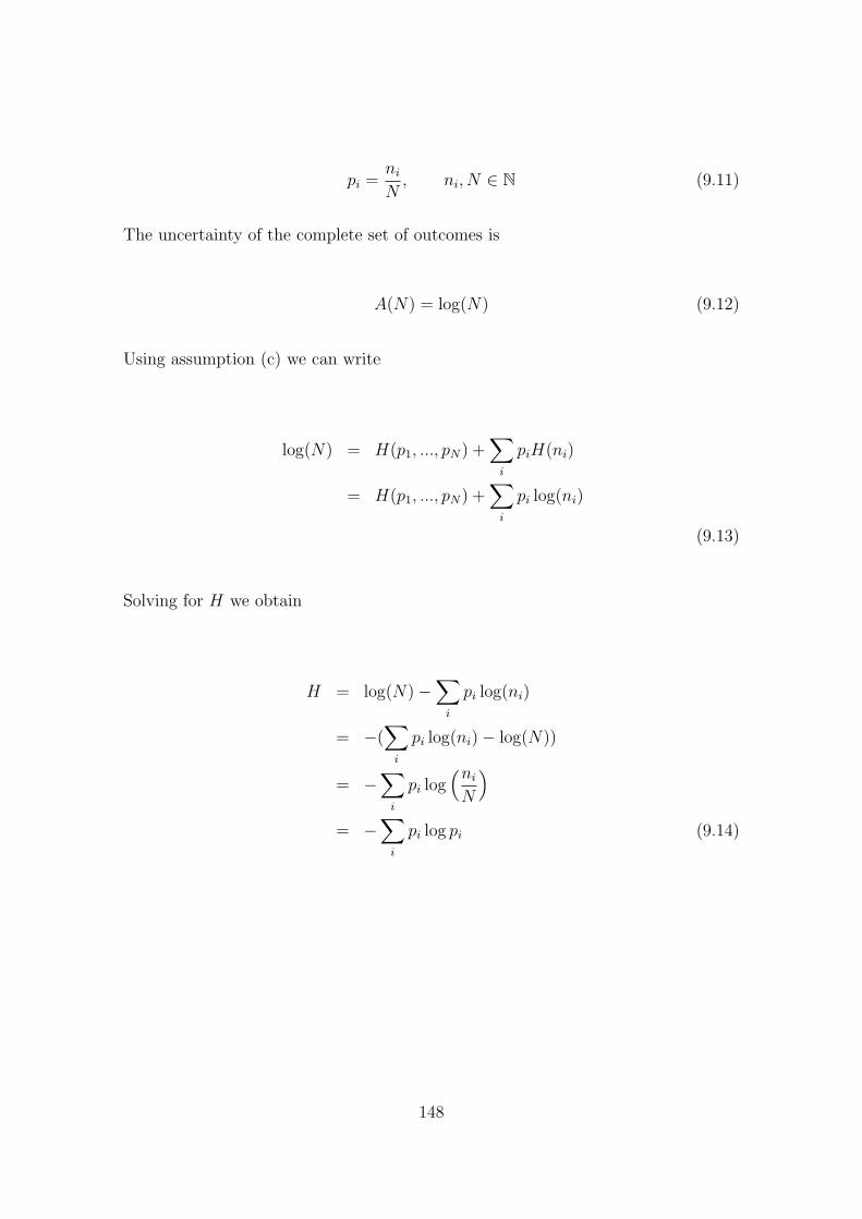
pi =niN, ni, N ∈ N (9.11)

The uncertainty of the complete set of outcomes is

A(N) = log(N) (9.12)

Using assumption (c) we can write

log(N) = H(p1, ..., pN) +∑i

piH(ni)

= H(p1, ..., pN) +∑i

pi log(ni)

(9.13)

Solving for H we obtain

H = log(N)−∑i

pi log(ni)

= −(∑i

pi log(ni)− log(N))

= −∑i

pi log(niN

)= −

∑i

pi log pi (9.14)

148

10 APPENDIX D - WAVE ENERGY IN THE BENJAMIN-BONA-

MAHONY EQUATION

The driven-damped regularized long wave equation (Benjamin-Bona-Mahony equa-

tion) is given by (HE; SALAT, 1989; REMPEL; CHIAN, 2007; HE, 1998; HE; CHIAN,

2004; HE; CHIAN, 2003; HE; CHIAN, 2005)

∂tu+ a∂txxu+ c∂xu+ fu∂xu = −νu− ε sin(κx− Ωt), (10.1)

where a, c, and f are constants, ν is a damping parameter, ε is the driver amplitude,

κ is the driver wavenumber and Ω is the driver frequency.

Ignoring the damping and external force we have (BENJAMIN et al., 1972; BENJAMIN,

1972)

∂tu+ a∂txxu+ c∂xu+ fu∂xu = 0. (10.2)

Multiplying Eq. (10.2) by u

u∂tu+ au∂txxu+ cu∂xu+ fu2∂xu = 0. (10.3)

Integrating Eq. (10.3) between x = −∞ and x =∞

∫ ∞−∞

u∂tudx+ a

∫ ∞−∞

u∂txxudx+ c

∫ ∞−∞

u∂xudx+ f

∫ ∞−∞

u2∂xudx = 0. (10.4)

The first term on the left-hand side of Eq. (10.4), after integrating by parts, can be

written as

∫u∂tudx =

1

2

∫∂tu

2dx (10.5)

The second term on the left-hand side of Eq. (10.4) can be written as

149

∫u∂x (∂x∂tu) dx = u (∂x∂tu)−

∫(∂xu) (∂x∂tu) dx (10.6)

The third term on the left-hand side of Eq. (10.4) can be written as

c

∫u∂xudx =

c

2

∫∂xu

2dx

=c

2u2 (10.7)

The fourth term on the left-hand side of Eq. (10.4) can be written as

f

∫u2∂xudx = f

(u3 − 2

∫u2∂xudx

)3f

∫u2∂xudx = fu3

f

∫u2∂xudx = f

u3

3(10.8)

Subtituting Eqs. (10.5), (10.6), (10.7) and (10.8) into Eq. (10.4)

1

2

∫ ∞−∞

∂tu2dx+ au∂x∂tu|∞−∞ − a

∫ ∞−∞

(∂xu) (∂x∂tu) dx+c

2u2∣∣∞−∞ + f

u3

3

∣∣∣∣∞−∞

= 0.

(10.9)

On the assumption that u, ∂xu and ∂x∂tu vanish as x → ±∞ (BENJAMIN, 1972),

Eq. (10.9) gives

150

1

2

∫ ∞−∞

∂tu2dx− a

∫ ∞−∞

(∂xu) [∂t (∂xu)] dx = 0

1

2

∫ ∞−∞

∂tu2dx− a

2

∫ ∞−∞

∂t (∂xu)2 dx = 0

∂t

[1

2

∫ ∞−∞

(u2 − a (∂xu)2) dx] = 0

1

2

∫ ∞−∞

[u2 − a (∂xu)2] dx = Cte (10.10)

Eq. (10.10) defines an invariant quantity of Eq. (10.2), the “wave energy” E (BEN-

JAMIN et al., 1972; BENJAMIN, 1972)

E =1

2

∫ ∞−∞

[u2 − a (∂xu)2] dx (10.11)

151

11 LIST OF PUBLICATIONS

•Koga, D., Chian, A. C.-L., Miranda, R. A., and Rempel, E. L. Intermit-

tent nature of solar wind turbulence near the Earth’s bow shock: phase

coherence and non-Gaussianity. Physical Review E, 75, 046401, 2007.

•Chian, A. C.-L. and Miranda, R. A.. Cluster and ACE observations of

phase synchronization in intermittent magnetic field turbulence: a compar-

ative study of shocked and unshocked solar wind. Annales Geophysicae, 27,

1789-1801, 2009.

•Miranda, R. A., Chian, A. C.-L., Dasso, S., Echer, E., Munoz, P. R.,

Trivedi, N. B., Tsurutani, B. T. and Yamada, M. Observation of non-

Gaussianity and phase synchronization in intermittent magnetic field tur-

bulence in the solar-terrestrial environment. Proceedings IAU symposium

No. 264, 363-368, 2010.

•Chian, A. C.-L., Miranda, R. A., Koga, D., Bolzan, M. J. A., Ramos, F.

M., and Rempel, E. L. Analysis of phase coherence in fully developed at-

mospheric turbulence: Amazon forest canopy. Nonlinear Processes in Geo-

physics, 15, 567-573, 2008.

•Rempel, E. L., Miranda, R. A., and Chian, A. C.-L. Spatiotemporal

intermittency and chaotic saddles in the regularized long-wave equation.

Physics of Fluids, 21, 074105, 2009.

•Chian, A. C.-L., Miranda, R. A., Rempel, E. L., Saiki, Y. and Yamada,

M. Amplitude-phase synchronization in chaotic saddles at the onset of per-

manent spatiotemporal chaos. Physics Review Letters, 2010 (submitted).

153

PUBLICACOES TECNICO-CIENTIFICAS EDITADAS PELO INPE

Teses e Dissertacoes (TDI) Manuais Tecnicos (MAN)

Teses e Dissertacoes apresentadas nosCursos de Pos-Graduacao do INPE.

Sao publicacoes de carater tecnico queincluem normas, procedimentos, in-strucoes e orientacoes.

Notas Tecnico-Cientıficas (NTC) Relatorios de Pesquisa (RPQ)

Incluem resultados preliminares depesquisa, descricao de equipamentos,descricao e ou documentacao de progra-mas de computador, descricao de sis-temas e experimentos, apresentacao detestes, dados, atlas, e documentacao deprojetos de engenharia.

Reportam resultados ou progressos depesquisas tanto de natureza tecnicaquanto cientıfica, cujo nıvel seja com-patıvel com o de uma publicacao emperiodico nacional ou internacional.

Propostas e Relatorios de Projetos(PRP)

Publicacoes Didaticas (PUD)

Sao propostas de projetos tecnico-cientıficos e relatorios de acompan-hamento de projetos, atividades e con-venios.

Incluem apostilas, notas de aula e man-uais didaticos.

Publicacoes Seriadas Programas de Computador (PDC)

Sao os seriados tecnico-cientıficos: bo-letins, periodicos, anuarios e anais deeventos (simposios e congressos). Con-stam destas publicacoes o InternacionalStandard Serial Number (ISSN), que eum codigo unico e definitivo para iden-tificacao de tıtulos de seriados.

Sao a sequencia de instrucoes ou codi-gos, expressos em uma linguagem deprogramacao compilada ou interpre-tada, a ser executada por um computa-dor para alcancar um determinado obje-tivo. Aceitam-se tanto programas fontequanto os executaveis.

Pre-publicacoes (PRE)

Todos os artigos publicados em periodi-cos, anais e como capıtulos de livros.

synchronization in intermittent turbulence and...

Documents